COUNTERFACTUAL GENERATIVE NETWORKS

Published as a conference paper at ICLR 2021

COUNTERFACTUAL GENERATIVE NETWORKS

Axel Sauer1,2 & Andreas Geiger1,2Autonomous Vision Group1Max Planck Institute for Intelligent Systems, Tubingen 2University of Tubingen{firstname.lastname}@tue.mpg.de

ABSTRACT

Neural networks are prone to learning shortcuts – they often model simple cor-relations, ignoring more complex ones that potentially generalize better. Priorworks on image classification show that instead of learning a connection to objectshape, deep classifiers tend to exploit spurious correlations with low-level tex-ture or the background for solving the classification task. In this work, we takea step towards more robust and interpretable classifiers that explicitly expose thetask’s causal structure. Building on current advances in deep generative modeling,we propose to decompose the image generation process into independent causalmechanisms that we train without direct supervision. By exploiting appropriateinductive biases, these mechanisms disentangle object shape, object texture, andbackground; hence, they allow for generating counterfactual images. We demon-strate the ability of our model to generate such images on MNIST and ImageNet.Further, we show that the counterfactual images can improve out-of-distributionrobustness with a marginal drop in performance on the original classification task,despite being synthetic. Lastly, our generative model can be trained efficiently ona single GPU, exploiting common pre-trained models as inductive biases.

1 INTRODUCTION

Deep neural networks (DNNs) are the main building blocks of many state-of-the-art machine learn-ing systems that address diverse tasks such as image classification (He et al., 2016), natural languageprocessing (Brown et al., 2020), and autonomous driving (Ohn-Bar et al., 2020). Despite the consid-erable successes of DNNs, they still struggle in many situations, e.g., classifying images perturbedby an adversary (Szegedy et al., 2013), or failing to recognize known objects in unfamiliar contexts(Rosenfeld et al., 2018) or from unseen poses (Alcorn et al., 2019).

Many of these failures can be attributed to dataset biases (Torralba & Efros, 2011) or shortcut learn-ing (Geirhos et al., 2020). The DNN learns the simplest correlations and tends to ignore more com-plex ones. This characteristic becomes problematic when the simple correlation is spurious, i.e., notpresent during inference. The motivational example of (Beery et al., 2018) considers the setting of aDNN that is trained to recognize cows in images. A real-world dataset will typically depict cows ongreen pastures in most images. The most straightforward correlation a classifier can learn to predictthe label ”cow” is hence the connection to a green, grass-textured background. Generally, this isnot a problem during inference as long as the test data follows the same distribution. However, ifwe provide the classifier an image depicting a purple cow on the moon, the classifier should stillconfidently assign the label ”cow.” Thus, if we want to achieve robust generalization beyond thetraining data, we need to disentangle possibly spurious correlations from causal relationships.

Distinguishing between spurious and causal correlations is one of the core questions in causalityresearch (Pearl, 2009; Peters et al., 2017; Scholkopf, 2019). One central concept in causality is theassumption of independent mechanisms (IM), which states that a causal generative process is com-posed of autonomous modules that do not influence each other. In the context of image classification(e.g., on ImageNet), we can interpret the generation of an image as a causal process (Kocaoglu et al.,2018; Goyal et al., 2019; Suter et al., 2019). We decompose this process into separate IMs, eachcontrolling one factor of variation (FoV) of the image. Concretely, we consider three IMs: onegenerates the object’s shape, the second generates the object’s texture, and the third generates thebackground. With access to these IMs, we can produce counterfactual images, i.e., images of unseencombinations of FoVs. We can then train an ensemble of invariant classifiers on the generated coun-

1


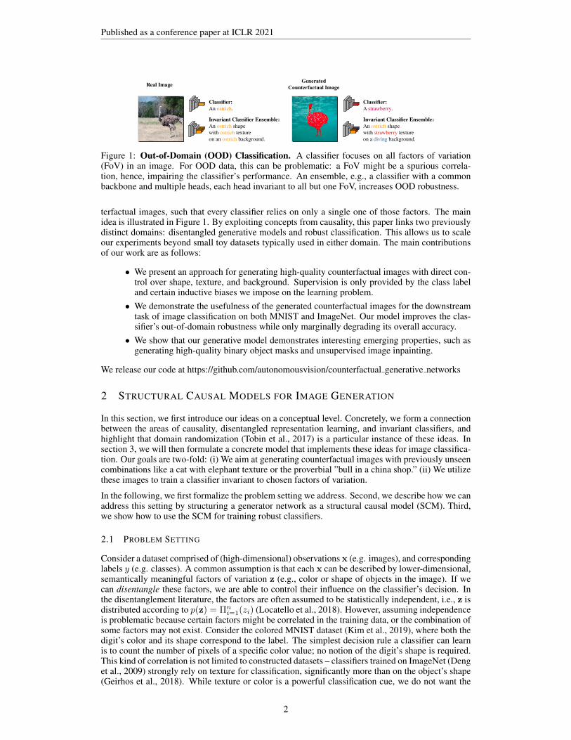
Invariant Classifier Ensemble:An ostrich shapewith ostrich textureon an ostrich background.

Classifier:An ostrich.

Invariant Classifier Ensemble:An ostrich shapewith strawberry textureon a diving background.

Classifier:A strawberry.

Real ImageGenerated

Counterfactual Image

Figure 1: Out-of-Domain (OOD) Classification. A classifier focuses on all factors of variation(FoV) in an image. For OOD data, this can be problematic: a FoV might be a spurious correla-tion, hence, impairing the classifier’s performance. An ensemble, e.g., a classifier with a commonbackbone and multiple heads, each head invariant to all but one FoV, increases OOD robustness.

terfactual images, such that every classifier relies on only a single one of those factors. The mainidea is illustrated in Figure 1. By exploiting concepts from causality, this paper links two previouslydistinct domains: disentangled generative models and robust classification. This allows us to scaleour experiments beyond small toy datasets typically used in either domain. The main contributionsof our work are as follows:

• We present an approach for generating high-quality counterfactual images with direct con-trol over shape, texture, and background. Supervision is only provided by the class labeland certain inductive biases we impose on the learning problem.

• We demonstrate the usefulness of the generated counterfactual images for the downstreamtask of image classification on both MNIST and ImageNet. Our model improves the clas-sifier’s out-of-domain robustness while only marginally degrading its overall accuracy.

• We show that our generative model demonstrates interesting emerging properties, such asgenerating high-quality binary object masks and unsupervised image inpainting.

We release our code at https://github.com/autonomousvision/counterfactual generative networks

2 STRUCTURAL CAUSAL MODELS FOR IMAGE GENERATION

In this section, we first introduce our ideas on a conceptual level. Concretely, we form a connectionbetween the areas of causality, disentangled representation learning, and invariant classifiers, andhighlight that domain randomization (Tobin et al., 2017) is a particular instance of these ideas. Insection 3, we will then formulate a concrete model that implements these ideas for image classifica-tion. Our goals are two-fold: (i) We aim at generating counterfactual images with previously unseencombinations like a cat with elephant texture or the proverbial ”bull in a china shop.” (ii) We utilizethese images to train a classifier invariant to chosen factors of variation.

In the following, we first formalize the problem setting we address. Second, we describe how we canaddress this setting by structuring a generator network as a structural causal model (SCM). Third,we show how to use the SCM for training robust classifiers.

2.1 PROBLEM SETTING

Consider a dataset comprised of (high-dimensional) observations x (e.g. images), and correspondinglabels y (e.g. classes). A common assumption is that each x can be described by lower-dimensional,semantically meaningful factors of variation z (e.g., color or shape of objects in the image). If wecan disentangle these factors, we are able to control their influence on the classifier’s decision. Inthe disentanglement literature, the factors are often assumed to be statistically independent, i.e., z isdistributed according to p(z) = Πn

i=1(zi) (Locatello et al., 2018). However, assuming independenceis problematic because certain factors might be correlated in the training data, or the combination ofsome factors may not exist. Consider the colored MNIST dataset (Kim et al., 2019), where both thedigit’s color and its shape correspond to the label. The simplest decision rule a classifier can learnis to count the number of pixels of a specific color value; no notion of the digit’s shape is required.This kind of correlation is not limited to constructed datasets – classifiers trained on ImageNet (Denget al., 2009) strongly rely on texture for classification, significantly more than on the object’s shape(Geirhos et al., 2018). While texture or color is a powerful classification cue, we do not want the

2

https://github.com/autonomousvision/counterfactual_generative_networks


classifier to ignore shape information completely. Therefore, we advocate a generative viewpoint.However, simply training, e.g., a disentangled VAE (Higgins et al., 2017) on this dataset, does notallow for generating data points of unseen combinations – the VAE cannot generate green zeros ifall zeros in the training data are red (see Appendix A for a visualization). We therefore propose anovel generative model which enables full control over several FoVs relevant for classification. Wethen train a classifier on these images while randomizing all factors but one. The classifier focuseson the non-randomized factor and becomes invariant wrt. the randomized ones.

2.2 STRUCTURAL CAUSAL MODELS

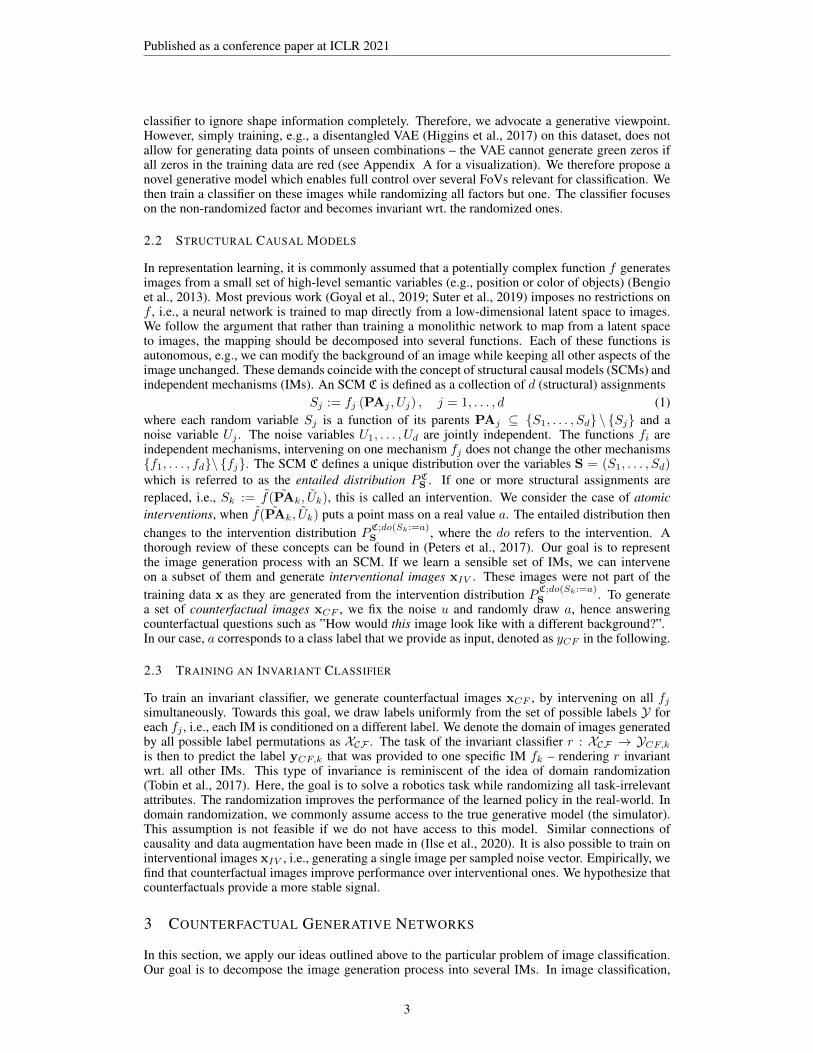
In representation learning, it is commonly assumed that a potentially complex function f generatesimages from a small set of high-level semantic variables (e.g., position or color of objects) (Bengioet al., 2013). Most previous work (Goyal et al., 2019; Suter et al., 2019) imposes no restrictions onf , i.e., a neural network is trained to map directly from a low-dimensional latent space to images.We follow the argument that rather than training a monolithic network to map from a latent spaceto images, the mapping should be decomposed into several functions. Each of these functions isautonomous, e.g., we can modify the background of an image while keeping all other aspects of theimage unchanged. These demands coincide with the concept of structural causal models (SCMs) andindependent mechanisms (IMs). An SCM C is defined as a collection of d (structural) assignments

Sj := fj (PAj , Uj) , j = 1, . . . , d (1)where each random variable Sj is a function of its parents PAj ⊆ {S1, . . . , Sd} \ {Sj} and anoise variable Uj . The noise variables U1, . . . , Ud are jointly independent. The functions fi areindependent mechanisms, intervening on one mechanism fj does not change the other mechanisms{f1, . . . , fd}\ {fj}. The SCM C defines a unique distribution over the variables S = (S1, . . . , Sd)which is referred to as the entailed distribution PC

S . If one or more structural assignments arereplaced, i.e., Sk := f(PAk, Uk), this is called an intervention. We consider the case of atomicinterventions, when f(PAk, Uk) puts a point mass on a real value a. The entailed distribution thenchanges to the intervention distribution PC;do(Sk:=a)

S , where the do refers to the intervention. Athorough review of these concepts can be found in (Peters et al., 2017). Our goal is to representthe image generation process with an SCM. If we learn a sensible set of IMs, we can interveneon a subset of them and generate interventional images xIV . These images were not part of thetraining data x as they are generated from the intervention distribution PC;do(Sk:=a)

S . To generatea set of counterfactual images xCF , we fix the noise u and randomly draw a, hence answeringcounterfactual questions such as ”How would this image look like with a different background?”.In our case, a corresponds to a class label that we provide as input, denoted as yCF in the following.

2.3 TRAINING AN INVARIANT CLASSIFIER

To train an invariant classifier, we generate counterfactual images xCF , by intervening on all fjsimultaneously. Towards this goal, we draw labels uniformly from the set of possible labels Y foreach fj , i.e., each IM is conditioned on a different label. We denote the domain of images generatedby all possible label permutations as XCF . The task of the invariant classifier r : XCF → YCF,k

is then to predict the label yCF,k that was provided to one specific IM fk – rendering r invariantwrt. all other IMs. This type of invariance is reminiscent of the idea of domain randomization(Tobin et al., 2017). Here, the goal is to solve a robotics task while randomizing all task-irrelevantattributes. The randomization improves the performance of the learned policy in the real-world. Indomain randomization, we commonly assume access to the true generative model (the simulator).This assumption is not feasible if we do not have access to this model. Similar connections ofcausality and data augmentation have been made in (Ilse et al., 2020). It is also possible to train oninterventional images xIV , i.e., generating a single image per sampled noise vector. Empirically, wefind that counterfactual images improve performance over interventional ones. We hypothesize thatcounterfactuals provide a more stable signal.

3 COUNTERFACTUAL GENERATIVE NETWORKS

In this section, we apply our ideas outlined above to the particular problem of image classification.Our goal is to decompose the image generation process into several IMs. In image classification,

3


cGAN

CGN

BigGAN

BigGAN

BigGAN

BigGAN U2-Net

U2-Net

Figure 2: Counterfactual Generative Network (CGN). Here, we illustrate the architecture used forthe ImageNet experiments. The CGN is split into four mechanisms, the shape mechanism fshape, thetexture mechanism ftext, the background mechanism fbg , and the composer C. Components withtrainable parameters are blue, components with fixed parameters are green. The primary supervisionis provided by an unconstrained conditional GAN (cGAN) via the reconstruction loss Lrec. ThecGAN is only used for training, as indicated by the dotted lines. Each mechanism takes as input thenoise vector u (sampled from a spherical Gaussian) and the label y (drawn uniformly from the setof possible labels Y) and minimizes its respective loss (Lshape, Ltext, and Lbg). To generate a setof counterfactual images, we sample u and then independently sample y for each mechanism.

there is generally one principal object in the image. Hence, we assume three IMs for this specifictask: object shape, object texture, and background. Our goal is to train the generator consisting ofthese mechanisms in an end-to-end manner. The inherent structure of the model allows us to generatemeaningful counterfactuals by construction. In the following, we describe the inductive biases weuse (network architectures, losses, pre-trained models) and how to train the invariant classifier. Werefer to the entire generative model using IMs as a Counterfactual Generative Network (CGN).

3.1 INDEPENDENT MECHANISMS

We assume the causal structure to be known, and consider three learned IMs for generating shape,texture, and background, respectively. The only difference between the MNIST variants and Ima-geNet is the background mechanism. For the MNIST variants, we can simplify the SCM to includea second texture mechanism instead of a dedicated background mechanism. There is no need for aglobally coherent background in the MNIST setting. An explicit formulation of both SCM is shownin Appendix B. In both cases, the learned IMs feed into another, fixed, IM: the composer. Anoverview of our CGN is shown in Figure 2. All IM-specific losses are optimized jointly end-to-end.For the experiments on ImageNet, we initialize each IM backbone with weights from a pre-trainedBigGAN-deep-256 (Brock et al., 2018), the current state-of-the-art for conditional image genera-tion. BigGAN has been trained as a single monolithic function; hence, it cannot generate images ofonly texture or only background, since these would be outside of the training domain.

Composition Mechanism. The function of the composer is not learned but defined analytically. Forthis work, we build on common assumptions from compositional image synthesis (Yang et al., 2017)and deploy a simple image formation model. Given the generated masks, textures and backgrounds,we composite the image xgen using alpha blending, denoted as C:

xgen = C(m, f ,b) = m� f + (1−m)� b (2)

where m is the mask (or alpha map), f is the foreground, and b is the background. The operator� denotes elementwise multiplication. While, in general, IMs may be stochastic (Eq. 1), we didnot find this to be necessary for the composer; therefore, we leave this mechanism deterministic.This fixed composition is a strong inductive bias in itself – the generator needs to generate realisticimages through this bottleneck. To optimize the composite image, we could use an adversarial lossbetween real and composite images. While applicable to simple datasets such as MNIST, we foundthat an adversarial approach does not scale well to more complex datasets like ImageNet. To get astronger and more stable supervisory signal, we, therefore, use an unconstrained, conditional GAN

4


(cGAN) to generate pseudo-ground-truth images xgt from noise u and label y. We feed the sameu and y into the IMs to generate xgen and minimize a reconstruction loss Lrec(xgt,xgen). Wefind a combination of L1 loss and perceptual loss (Johnson et al., 2016) to work well. Note thatduring training, we utilize the same noise u and label y to reconstruct the image generated by thecGAN. However, at inference time, we generate counterfactual images by randomizing both u andy separately per mechanism.

Shape Mechanism. We model the shape using a binary mask predicted by shape IM fshape, where0 corresponds to the background and 1 to the object. Effectively, this mechanism implements fore-ground segmentation. The loss is comprised of two terms: Lbinary and Lmask. Lbinary is the pixel-wise binary entropy of the mask; hence, minimizing it forces the output to be close to either 0 or 1.Lmask prohibits trivial solutions, i.e., masks with all 0’s or 1’s that are outside of a defined interval(see Appendix C for details). As we utilize a BigGAN backbone for our ImageNet-Experiments, weneed to extract a binary mask from the backbone’s output. Therefore, we add a pre-trained U2-Net(Qin et al., 2020) as a head on top of the BigGAN backbone. The U2-Net was trained for salientobject detection on DUTS-TR (10553 images) (Wang et al., 2017). Hence, it is class agnostic; itgenerates an object mask for a salient object in the image. While the U2-Net presents a strong biastowards binary object masks, it does not fully solve the task at hand as it captures non-class specificparts (e.g., parts of trees in an elephant-class picture, see Figure 5). By fine-tuning the BigGANbackbone, we learn to generate images of the relevant part with exaggerated features to increasesaliency. We refer to these as pre-masks m.

Texture Mechanism. The texture mechanism ftext is responsible for generating the foregroundobject’s appearance, while not capturing any object shape or background cues. For MNIST, we usean architectural bias – an additional layer before the final output. This layer spatially divides its inputinto patches and randomly rearranges them, similar to a shuffled sliding puzzle. This conceptuallysimple idea does not work on ImageNet, as we want to preserve local object structure, e.g., theposition of an eye. We, therefore, sample patches from the full composite image and concatenatethem into a grid. We denote this patch grid as pg. The patches are sampled from regions where themask values are highest (hence, the object is likely located). We then minimize a perceptual lossbetween the foreground f (the output of ftext) and the patchgrid: Ltext(f ,pg). Over training, thebackground gradually transforms into object texture, resulting in texture maps, as shown in Figure5. More details can be found in Appendix C.

Background Mechanism. The background mechanism fbg needs to capture the background’sglobal structure while the object must be removed and inpainted realistically. However, we foundthat we cannot use standard inpainting techniques because classical methods (Barnes et al., 2009)slow down training too much, and deep learning methods (Liu et al., 2018) do not work well onsynthetic data because of the domain shift. Instead, we exploit the same U2-Net as used for theshape mechanism fshape. Again, we feed the output of the BigGAN backbone through the U2-Netwith fixed weights. However, this time, we minimize the predicted saliency. Over the progress oftraining, this leads to the object shrinking and finally disappearing, while the model learns to inpaintthe object region (see Figure 5 and Appendix E). We refer to this loss as Lbg . We attribute this loss’ssuccess mainly the powerful pre-trained backbone network. BigGAN is already able to generateobjects on realistic backgrounds; it only needs to unlearn the object generation.

3.2 GENERATING COUNTERFACTUALS TO TRAIN CLASSIFIERS

After training our CGN, each IM network has learned a class-conditional distribution over shapes,textures, or backgrounds. By randomizing the label input y and noise u of each network, we cangenerate counterfactual images. The number of possible combinations is the number of classes to thepower of the number of IM’s. For ImageNet, this is 10003. The amount of possible images is evenlarger since we learn distributions, i.e., we can generate a nearly unlimited variety of shapes, textures,and backgrounds, per class. We train on both real and counterfactual images. For MNIST, morecounterfactual images always increase the test domain results; see the ablation study in AppendixA.3. On Imagenet, we provide evenly sized batches of real and counterfactual images; i.e., we usea ratio of 1. A ratio below 1 leads to inferior performance; a ratio above 1 leads to longer trainingtimes without an increase in performance. Similar results were reported for training on BigGANsamples in Ravuri & Vinyals (2019).

5


Generated Counterfactual ImagesReal Images

WildlifeDouble-ColoredColored WildlifeDouble-ColoredColored

Figure 3: MNISTs. Left: Samples of the different MNIST variations (for brevity, we show only thefirst four classes). Right: Counterfactual samples generated by our CGN. Note that the CGN learnedclass-conditional distributions, i.e., it generates varying shapes, colors, and textures.

4 EXPERIMENTS

Our experiments aim to answer the following questions: (i) Does our approach reliably learn thedisentangled IMs on datasets of different complexity? (ii) Which inductive biases are necessary toachieve this? (iii) Do counterfactual images enable training invariant classifiers? We first apply ourapproach to different versions of MNIST: colored-, double-colored- and Wildlife-MNIST (detailsabout their generation are in Appendix A.2). The label is encoded in the digit shape, foregroundcolor or texture, and the background color or texture, see Figure 3. Our work focuses on a settingwhere the spurious signal is a strong predictor of the label; hence we assume a correlation strengthof at least 90 % between signal and label in our simulated environments. This assumption is in linewith latest related work on visual bias (Goyal et al., 2019; Wang et al., 2020), which considers astrong correlation to be above 95 %. We then scale our approach to ImageNet and demonstrate thatwe can improve the robustness of ImageNet classifiers. Implementation details about architectures,loss parameters, and hyperparameters can be found in Appendix C.

4.1 DOES OUR APPROACH LEARN THE DISENTANGLED INDEPENDENT MECHANISMS?

Standard metrics like the Inception Score (IS) (Salimans et al., 2016) are not applicable since thecounterfactual images are outside of the natural image domain. We thus focus on qualitative resultsin this section. For a quantitative analysis, we refer the reader to Section 4.3 where we analyze theaccuracy, robustness, and invariance of classifiers trained on the generated counterfactual data.

MNISTs. The generated counterfactual images are shown in Figure 3 (right). None of the counter-factual combinations were present in the training data. We can see that CGN successfully generateshigh-quality counterfactuals. The results on Wildlife MNIST are surprisingly good, considering thatthe object texture is only observable on the relatively thin digits. Nevertheless, the texture IM learnsto generate realistic textures. All experiments on MNIST are done without pre-training any network.

ImageNet. As shown in Figure 4, our CGN generates counterfactuals of high visual fidelity. Wetrain a single CGN for all 1000 classes. We also find an unexpected benefit of our approach. In someinstances, the composite images eliminate structural artifacts of the original BigGAN images, suchas surplus legs, as shown in Figure 5. We hypothesize that fshape learns a general shape conceptper class, resulting in outliers, like elephants with eight legs, being smoothed out. We show moresamples, individual IM outputs, and interpolations in Appendix D. The CGN can fail to producehigh-quality texture maps for very small objects, e.g., for a bird high up in the sky, the texture mapwill still show large portions of the sky. Also, in some instances, a residue of the object is left onthe background, e.g., a dog snout. For generating counterfactual images, this is not a problem asa different object will cover the residue. Lastly, the enforced constraints can lead to a reductionin realism of the composite images xgen compared to the original BigGAN samples. We showexamples and propose solutions for these problems in Appendix F.

4.2 WHICH INDUCTIVE BIASES ARE NEEDED TO ACHIEVE DISENTANGLEMENT?

We employ two kinds of biases: pre-training of modules and IM-specific losses. We find that pre-training is not necessary for our experiments on MNIST. However, when scaling to ImageNet, pow-erful pre-trained models are key for achieving good results. Furthermore, this allows to train the

6


Shape

Texture

Background

red wine cottontail rabbit pirate ship triumphal arch mushroom hyena dog

carbonara head cabbage banana Indian elephant barrel school bus

baseball valley bittern (bird) viaduct grey whale snorkel

Figure 4: ImageNet Counterfactuals. The CGN successfully learns the disentangled shape, texture,and background mechanisms, and enables the generation of numerous permutations thereof.

Figure 5: Individual IM Outputs over Training. We show pre-masks m, masks m, foregrounds f ,and backgrounds b. The arrows indicate the beginning and end of the training. The initial output ofthe pre-trained models is gradually transformed while the composite image only marginally changes.

whole CGN on a single NVIDIA GTX 1080Ti within 12 hours, in contrast to BigGAN, which wastrained on a Google TPU v3 Pod with 512 cores for up to 48 hours. To investigate each loss’ influ-ence, we disable one loss at a time and measure its influence on the quality of the composite images.The composite images are on the image manifold, hence, we can calculate their Inception score (IS).As we train with pseudo ground truth, the performance of the unconstrained BigGAN is a naturalupper bound. The used model reaches an IS of 202.9. To measure if the CGN collapsed duringtraining, we monitor the mean value of the generated mask µmask. A µmask close to 1 means thatftext is not training. Instead, it generates the output of the pre-trained BigGAN, hence, a mask of1’s trivially minimizes the reconstruction loss Lrec(xgt,xgen). The same is true for µmask close to0 and fbg . The results in Table 1 indicate that each loss is necessary, and jointly optimizing all ofthem end-to-end is needed for a high IS without a collapse of µmask. Removing Lshape, leads to badquality masks (non-binary, only partially capturing the object). This results in a low IS since objecttexture and background get mixed in the composited image. Not using either Ltext or Lbg resultsin a high IS (as the output is close to the original BigGAN output), but a collapse of µmask. Themechanisms do not disentangle their respective signal. Finally, disabling Lrec leads to a very lowIS, since the IMs can optimize their respective loss without any constraint on the composite image.We show the evolution and collapse of the masks over training in Appendix G.

4.3 DO COUNTERFACTUAL IMAGES ENABLE TRAINING OF INVARIANT CLASSIFIERS?

The following experiments investigate if we can instill invariance into a classifier. We performexperiments on the MNIST variants, a cue-conflict dataset, and an OOD version of ImageNet.

MNIST Classification. In the training domain, shapes, colors, and textures are correlated with theclass label. In the test domain, only the shapes correspond to the correct class. We compare to currentapproaches for training invariant classifiers: IRM (Arjovsky et al., 2019) and Learning-not-to-learn(LNTL) (Kim et al., 2019). For a detailed description we refer to Appendix C. Original + CGN isadditionally trained on counterfactual data to predict the input labels of the shape IM. Original +GAN is a baseline that is trained on real and generated, non-counterfactual samples. IRM considersa signal to be causal if it is stable across several environments. We train IRM on 2 environments (90% and 100 % correlation) or 5 environments (90 %, 92.5 %, 95 %, 97.5 %, and 100% correlation).LNTL considers color to be spurious, whereas we assume (complementary) that shapes are causal.

Alternatively, we can follow the same assumption as IRM with an additional causal identification

7


Lshape Ltext Lbg Lrec IS ⇑ µmask

7 3 3 3 85.9 0.2± 0.2 %3 7 3 3 198.4 0.9± 0.1 %3 3 7 3 195.6 0.1± 0.1 %3 3 3 7 38.39 0.3± 0.2 %3 3 3 3 130.2 0.3± 0.2%

BigGAN (Upper Bound) 202.9 -

Table 1: Loss Ablation Study. Weturn off one loss at a time. Valuesindicating mask collapse are red.

colored MNIST double-colored MNIST Wildlife MNISTTrain Acc ⇑ Test Acc ⇑ Train Acc ⇑ Test Acc ⇑ Train Acc ⇑ Test Acc ⇑

Original 99.5 % 35.9 % 100.0 % 10.3 % 100.0 % 10.1 %IRM (2 Envs) 99.6 % 59.8 % 100.0 % 67.7 % 99.9 % 11.3 %IRM (5 Envs) - - 99.9 % 78.9 % 99.8 % 76.8 %

LNTL 99.3 % 81.8 % 98.7 % 69.9 % 99.9 % 11.5 %Original + GAN 99.8 % 40.7 % 100.0 % 10.8 % 100.0 % 10.4 %Original + CGN 99.7 % 95.1 % 97.4 % 89.0 % 99.2 % 85.7 %

Table 2: MNISTs Classification. In the test set, colors andtextures are randomized, only the digit’s shape corresponds tothe class label. Random performance is at 10%.

Trained on Shape Bias top-1 IN Acc ⇑ top-5 IN Acc ⇑

IN 21.39 % 76.13 % 92.86 %SIN 81.37 % 60.18 % 82.62 %IN + SIN 34.65 % 74.59 % 90.03 %

IN + CGN/Shape 54.82 %73.98 % 91.71 %IN + CGN/Text 16.67 %

IN + CGN/Bg 22.89 %

Table 3: Shape vs. Texture. We can controlthe classifier’s shape or texture preference.

Top-1 Test Accuracies

Trained on IN-9 ⇑ Mixed-Same ⇑ Mixed-Rand ⇑ BG-Gap ⇓

IN 95.6% 86.2% 78.9% 7.3%SIN 89.2 % 73.1 % 63.7 % 9.4 %IN + SIN 94.7 % 85.9 % 78.5 % 7.4 %Mixed-Rand 73.3% 71.5% 71.3% 0.2 %IN + CGN 94.2 % 83.4 % 80.1 % 3.3 %

Table 4: Accuracies on IN-9. The reported accu-racies are all obtained using a Resnet-50.

step, see Appendix H. The results in Table 2 confirm that training on counterfactual data leads toclassifiers that are invariant to the spurious signals. We hypothesize that the difference betweenenvironments may be hard to pick up for IRM, especially if only a few are available. We find thatwe can further improve IRM’s performance by adding more environments. However, continuallyincreasing the number of environments is an unrealistic premise and only feasible in simulatedenvironments. Our results indicate that LNTL and IRM have trouble scaling to more complex data.

Texture vs. Shape Bias. The Cue Conflict dataset consists of images generated using iterative styletransfer (Gatys et al., 2015) between a texture and a content image. A high shape bias correspondsto classification according to the content label and vice versa for texture. Their approach is trainedon stylized ImageNet (SIN), either as a drop-in for ImageNet (IN) or as augmentation. We usea classifier ensemble, i.e., a classifier with a common backbone and multiple heads, each headinvariant to all but one FoV. We average the predicted log-probabilies of each head for the finaloutput of the ensemble. We conduct all experiments using a Resnet-50 architecture. As shown inTable 3, we can influence the individual bias of each classifier head without significant degradationin the ensemble’s performance.

Invariance over Backgrounds. Xiao et al. (2020) propose the BG-Gap to measure a classifier’sdependence on the background signal. Based on ImageNet-9 (IN-9), a subset of ImageNet with9 coarse-grained classes, they build synthetic datasets. For Mixed-Rand, the backgrounds are ran-domized, while the object remains unchanged, hence background an class are decorrelated. ForMixed-Same they sample class-consistent backgrounds. The BG-Gap is the difference in perfor-mance between the two. Training on IN or SIN does not make it possible to disentangle and omitthe background signal, as shown in Table 4. Directly training on Mixed-Rand leads to a drop in per-formance on the original data which might be due to the smaller training dataset. We can generateunlimited data of this type, hence, we are able to reduce the gap while achieving high accuracy onIN-9. However, a gap to a fully invariant classifier remains. We partially attribute this to the generalremaining domain gap between generated and real images.

5 RELATED WORK

Our work is related to disentangled representation learning and the training of invariant classifiers.

Disentangled Representation Learning. A recent line of work in image synthesis aims to learndisentangled features for controlling the image generation process (Chen et al., 2016; Higgins et al.,2017; Liao et al., 2020). The challenge of the task is that the underlying factors can be highlycorrelated. Closely related to our work is (Li et al., 2020), which aims to disentangle background,shape, pose, and texture, using object bounding boxes for supervision. Their methods assumes

8


images of a single object category (e.g. birds). We scale our approach to all classes of ImageNetwhich enables us to generate inter-class counterfactuals. A recent research direction explores thediscovery of interpretable directions in GANs trained on ImageNet (Plumerault et al., 2020; Voynov& Babenko, 2020; Peebles et al., 2020). These approaches do not allow for generating counterfactualimages. Kocaoglu et al. (2018) train two separate generative models, one generating binary featurelabels (mustache, young), the other generating images conditioned on these labels. Their model cancreate images of previously unseen combinations of attributes, e.g., women with mustaches. Thisapproach assumes a data set with fine-grained labels; hence it would not be suited to our applicationsince labels for high-level concepts like shape are hard to obtain. Besserve et al. (2019) also leveragethe idea of independent mechanisms to discover modularity in pre-trained generative models. Theirapproach does not allow for direct control of image attributes. Lastly, methods for causal generativemodeling utilizing competing experts (von Kugelgen et al., 2020) have been demonstrated on toydatasets only. Further, none of the works above aim to use the generated images to improve upon adownstream task such as image classification.

Invariant Classification. Current approaches do not take an underlying causal model into account.Instead, they rely on different assumptions. Arjovsky et al. (2019) assume that the training datais collected into separate environments (e.g. different measurement circumstances). Correlationsthat are stable across environments are considered to be causal. Kim et al. (2019) aim to learn fea-tures that are uninformative of a given bias (spurious) signal. As mentioned above, attaining labelsfor shape or texture is expensive and not straight-forward. A recent strand of work is concernedwith data augmentation for improving invariance against spurious correlations. Shetty et al. (2020)propose to train object detectors on generated semantic adversarial data, effectively reducing the tex-ture dependency of their model. Their finding is in line with (Geirhos et al., 2018) that proposes totransfer the style of paintings onto images and use them for data augmentation. These approaches,however, do not allow to choose the specific signal we want invariance for, e.g., the background.The use of counterfactual data has been previously explored in natural language inference (Kaushiket al., 2020) and visual question answering (Teney et al., 2020).

6 DISCUSSION

We assume that an image can be neatly distinguished into a class foreground and backgroundthroughout this work. This assumption breaks once we consider more complex scenes with differ-ent object instances or for tasks without a clear foreground-background distinction, e.g., in medicalimages. The composition mechanism is a powerful bias, and crucial to making our model work.In other domains, equally strong biases may need to be identified to enable learning the SCM. Anexciting research direction is to explore different configurations of IMs to tackle these challenges.

The additional constraints that we enforce during the CGN training lead to a reduced realism, asevidenced by the lower IS. We also find that our generated images can significantly influence aclassifier’s preference, but their quality is not high enough to improve performance on ImageNet.However, even state-of-the-art generative models (with higher IS) are not good enough yet to gen-erate data for training competitive ImageNet classifiers (Ravuri & Vinyals, 2019).

Lastly, in our experiments, we assume the causal structure to be known. This assumption is sub-stantially stronger than the ones in more general standard disentanglement frameworks (Chen et al.,2016; Higgins et al., 2017). A possible extension to our work could leverage causal discovery toisolate IMs in a domain-agnostic manner, e.g., via meta-learning (Bengio et al., 2020). On the otherhand, the definition of a causal structure and the approximation through IMs may be a principledway to integrate domain knowledge into a machine learning system, The need for better interfacesto integrate domain knowledge has recently been highlighted in (D’Amour et al., 2020).

7 CONCLUSION

In this work, we apply ideas from causality to generative modeling and the training of invariant clas-sifiers. We structure a generative network into independent mechanisms to generate counterfactualimages useful for training classifiers. With the use of several inductive biases, we demonstrate ourapproach on various MNIST variants as well as ImageNet. Our ideas are orthogonal to advances ingenerative modeling - with advances therein, our obtained results will further improve.

9


ACKNOWLEDGMENTS

We acknowledge the financial support by the BMWi in the project KI Delta Learning (project num-ber 19A19013O). Andreas Geiger was supported by the ERC Starting Grant LEGO-3D (850533).We would like to thank Yiyi Lao, Michael Niemeyer, and Elie Aljalbout for comments on an earlierpaper draft and Songyou Peng, Michael Oechsle, and Kashyap Chitta for last-minute proofreading.We would also like to thank Vanessa Sauer for her general support and constructive criticism on thegenerated counterfactuals in earlier stages.

REFERENCES

Michael A Alcorn, Qi Li, Zhitao Gong, Chengfei Wang, Long Mai, Wei-Shinn Ku, and Anh Nguyen.Strike (with) a pose: Neural networks are easily fooled by strange poses of familiar objects. InCVPR, 2019.

Martin Arjovsky, Leon Bottou, Ishaan Gulrajani, and David Lopez-Paz. Invariant risk minimization.arXiv preprint arXiv:1907.02893, 2019.

Connelly Barnes, Eli Shechtman, Adam Finkelstein, and Dan B Goldman. Patchmatch: A random-ized correspondence algorithm for structural image editing. In ACM TOG, 2009.

Sara Beery, Grant Van Horn, and Pietro Perona. Recognition in terra incognita. In ECCV, 2018.

Yoshua Bengio, Aaron Courville, and Pascal Vincent. Representation learning: A review and newperspectives. TPAMI, 2013.

Yoshua Bengio, Tristan Deleu, Nasim Rahaman, Rosemary Ke, Sebastien Lachapelle, Olexa Bila-niuk, Anirudh Goyal, and Christopher Pal. A meta-transfer objective for learning to disentanglecausal mechanisms. In ICLR, 2020.

Michel Besserve, Arash Mehrjou, Remy Sun, and Bernhard Scholkopf. Counterfactuals uncover themodular structure of deep generative models. In ICLR, 2019.

Andrew Brock, Jeff Donahue, and Karen Simonyan. Large scale gan training for high fidelity naturalimage synthesis. In ICLR, 2018.

Tom B Brown, Benjamin Mann, Nick Ryder, Melanie Subbiah, Jared Kaplan, Prafulla Dhariwal,Arvind Neelakantan, Pranav Shyam, Girish Sastry, Amanda Askell, et al. Language models arefew-shot learners. arXiv preprint arXiv:2005.14165, 2020.

Xi Chen, Yan Duan, Rein Houthooft, John Schulman, Ilya Sutskever, and Pieter Abbeel. Infogan:Interpretable representation learning by information maximizing generative adversarial nets. InNeurIPS, 2016.

M. Cimpoi, S. Maji, I. Kokkinos, S. Mohamed, , and A. Vedaldi. Describing textures in the wild. InCVPR, 2014.

Alexander D’Amour, Katherine Heller, Dan Moldovan, Ben Adlam, Babak Alipanahi, Alex Beutel,Christina Chen, Jonathan Deaton, Jacob Eisenstein, Matthew D. Hoffman, Farhad Hormozdi-ari, Neil Houlsby, Shaobo Hou, Ghassen Jerfel, Alan Karthikesalingam, Mario Lucic, Yian Ma,Cory McLean, Diana Mincu, Akinori Mitani, Andrea Montanari, Zachary Nado, Vivek Natarajan,Christopher Nielson, Thomas F. Osborne, Rajiv Raman, Kim Ramasamy, Rory Sayres, JessicaSchrouff, Martin Seneviratne, Shannon Sequeira, Harini Suresh, Victor Veitch, Max Vladymy-rov, Xuezhi Wang, Kellie Webster, Steve Yadlowsky, Taedong Yun, Xiaohua Zhai, and D. Sculley.Underspecification presents challenges for credibility in modern machine learning. arXiv preprintarXiv:2011.03395, 2020.

Jia Deng, Wei Dong, Richard Socher, Li-Jia Li, Kai Li, and Li Fei-Fei. Imagenet: A large-scalehierarchical image database. In CVPR, 2009.

Leon A Gatys, Alexander S Ecker, and Matthias Bethge. A neural algorithm of artistic style. arXivpreprint arXiv:1508.06576, 2015.

10


Robert Geirhos, Patricia Rubisch, Claudio Michaelis, Matthias Bethge, Felix A Wichmann, andWieland Brendel. Imagenet-trained cnns are biased towards texture; increasing shape bias im-proves accuracy and robustness. In ICLR, 2018.

Robert Geirhos, Jorn-Henrik Jacobsen, Claudio Michaelis, Richard Zemel, Wieland Brendel,Matthias Bethge, and Felix A Wichmann. Shortcut learning in deep neural networks. arXivpreprint arXiv:2004.07780, 2020.

Ian Goodfellow, Jean Pouget-Abadie, Mehdi Mirza, Bing Xu, David Warde-Farley, Sherjil Ozair,Aaron Courville, and Yoshua Bengio. Generative adversarial nets. In NeurIPS, 2014.

Yash Goyal, Amir Feder, Uri Shalit, and Been Kim. Explaining classifiers with causal concept effect(CACE). arXiv preprint arXiv:1907.07165, 2019.

Kaiming He, Xiangyu Zhang, Shaoqing Ren, and Jian Sun. Deep residual learning for image recog-nition. In CVPR, 2016.

Irina Higgins, Loic Matthey, Arka Pal, Christopher Burgess, Xavier Glorot, Matthew Botvinick,Shakir Mohamed, and Alexander Lerchner. beta-vae: Learning basic visual concepts with aconstrained variational framework. In ICLR, 2017.

Maximilian Ilse, Jakub M Tomczak, and Patrick Forre. Designing data augmentation for simulatinginterventions. arXiv preprint arXiv:2005.01856, 2020.

Justin Johnson, Alexandre Alahi, and Li Fei-Fei. Perceptual losses for real-time style transfer andsuper-resolution. In ECCV, 2016.

Divyansh Kaushik, Eduard Hovy, and Zachary C Lipton. Learning the difference that makes adifference with counterfactually-augmented data. In ICLR, 2020.

Byungju Kim, Hyunwoo Kim, Kyungsu Kim, Sungjin Kim, and Junmo Kim. Learning not to learn:Training deep neural networks with biased data. In CVPR, 2019.

Diederik P Kingma and Jimmy Ba. Adam: A method for stochastic optimization. arXiv preprintarXiv:1412.6980, 2014.

Murat Kocaoglu, Christopher Snyder, Alexandros G Dimakis, and Sriram Vishwanath. Causalgan:Learning causal implicit generative models with adversarial training. In ICLR, 2018.

Yuheng Li, Krishna Kumar Singh, Utkarsh Ojha, and Yong Jae Lee. Mixnmatch: Multifactor disen-tanglement and encoding for conditional image generation. In CVPR, 2020.

Yiyi Liao, Katja Schwarz, Lars Mescheder, and Andreas Geiger. Towards unsupervised learning ofgenerative models for 3d controllable image synthesis. In CVPR, 2020.

Guilin Liu, Fitsum A Reda, Kevin J Shih, Ting-Chun Wang, Andrew Tao, and Bryan Catanzaro.Image inpainting for irregular holes using partial convolutions. In ECCV, 2018.

Francesco Locatello, Stefan Bauer, Mario Lucic, Sylvain Gelly, Bernhard Scholkopf, and OlivierBachem. Challenging common assumptions in the unsupervised learning of disentangled repre-sentations. In ICML, 2018.

Eshed Ohn-Bar, Aditya Prakash, Aseem Behl, Kashyap Chitta, and Andreas Geiger. Learning situ-ational driving. In CVPR, 2020.

Judea Pearl. Causality. Cambridge University Press, 2009.

William Peebles, John Peebles, Jun-Yan Zhu, Alexei A. Efros, and Antonio Torralba. The hessianpenalty: A weak prior for unsupervised disentanglement. In ECCV, 2020.

Jonas Peters, Dominik Janzing, and Bernhard Scholkopf. Elements of causal inference. The MITPress, 2017.

Antoine Plumerault, Herve Le Borgne, and Celine Hudelot. Controlling generative models withcontinuous factors of variations. In ICLR, 2020.

11


Xuebin Qin, Zichen Zhang, Chenyang Huang, Masood Dehghan, Osmar R Zaiane, and MartinJagersand. U2-net: Going deeper with nested u-structure for salient object detection. PatternRecognition, 2020.

Suman Ravuri and Oriol Vinyals. Seeing is not necessarily believing: Limitations of biggans fordata augmentation. In ICLR Workshop LLD, 2019.

Amir Rosenfeld, Richard Zemel, and John K Tsotsos. The elephant in the room. arXiv preprintarXiv:1808.03305, 2018.

Tim Salimans, Ian Goodfellow, Wojciech Zaremba, Vicki Cheung, Alec Radford, and Xi Chen.Improved techniques for training gans. In NeurIPS, 2016.

Bernhard Scholkopf. Causality for machine learning. arXiv preprint arXiv:1911.10500, 2019.

Rakshith Shetty, Mario Fritz, and Bernt Schiele. Towards automated testing and robustification bysemantic adversarial data generation. In ECCV, 2020.

Raphael Suter, Djordje Miladinovic, Bernhard Scholkopf, and Stefan Bauer. Robustly disentangledcausal mechanisms: Validating deep representations for interventional robustness. In ICML, 2019.

Christian Szegedy, Wojciech Zaremba, Ilya Sutskever, Joan Bruna, Dumitru Erhan, Ian Goodfellow,and Rob Fergus. Intriguing properties of neural networks. arXiv preprint arXiv:1312.6199, 2013.

Damien Teney, Ehsan Abbasnedjad, and Anton van den Hengel. Learning what makes a differencefrom counterfactual examples and gradient supervision. In ECCV, 2020.

Josh Tobin, Rachel Fong, Alex Ray, Jonas Schneider, Wojciech Zaremba, and Pieter Abbeel. Do-main randomization for transferring deep neural networks from simulation to the real world. InIROS, 2017.

Antonio Torralba and Alexei A Efros. Unbiased look at dataset bias. In CVPR, 2011.

Julius von Kugelgen, Ivan Ustyuzhaninov, Peter Gehler, Matthias Bethge, and Bernhard Scholkopf.Towards causal generative scene models via competition of experts. In ICLR Workshop CLDM,2020.

Andrey Voynov and Artem Babenko. Unsupervised discovery of interpretable directions in the ganlatent space. arXiv preprint arXiv:2002.03754, 2020.

Lijun Wang, Huchuan Lu, Yifan Wang, Mengyang Feng, Dong Wang, Baocai Yin, and Xiang Ruan.Learning to detect salient objects with image-level supervision. In CVPR, 2017.

Zeyu Wang, Klint Qinami, Ioannis Christos Karakozis, Kyle Genova, Prem Nair, Kenji Hata, andOlga Russakovsky. Towards fairness in visual recognition: Effective strategies for bias mitigation.In CVPR, 2020.

Kai Xiao, Logan Engstrom, Andrew Ilyas, and Aleksander Madry. Noise or signal: The role ofimage backgrounds in object recognition. arXiv preprint arXiv:2006.09994, 2020.

Jianwei Yang, Anitha Kannan, Dhruv Batra, and Devi Parikh. Lr-gan: Layered recursive generativeadversarial networks for image generation. arXiv preprint arXiv:1703.01560, 2017.

12


APPENDIX A MNIST VARIANTS

A.1 VARIATIONAL AUTOENCODERS ON COLORED MNIST

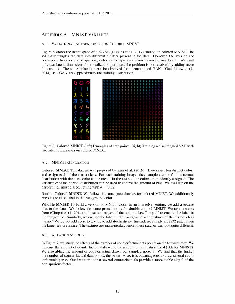
Figure 6 shows the latent space of a β-VAE (Higgins et al., 2017) trained on colored MNIST. TheVAE disentangles the data into different clusters present in the data. However, the axes do notcorrespond to color and shape, i.e., color and shape vary when traversing one latent. We usedonly two latent dimensions for visualization purposes; the problem is not resolved by adding moredimensions. The same behaviour can be observed for unconstrained GANs (Goodfellow et al.,2014), as a GAN also approximates the training distribution.

Figure 6: Colored MNIST. (left) Examples of data points. (right) Training a disentangled VAE withtwo latent dimensions on colored MNIST.

A.2 MNISTS GENERATION

Colored MNIST. This dataset was proposed by Kim et al. (2019). They select ten distinct colorsand assign each of them to a class. For each training image, they sample a color from a normaldistribution with the class color as the mean. In the test set, the colors are randomly assigned. Thevariance σ of the normal distribution can be used to control the amount of bias. We evaluate on thehardest, i.e., most biased, setting with σ = 0.02.

Double-Colored MNIST. We follow the same procedure as for colored MNIST. We additionallyencode the class label in the background color.

Wildlife MNIST. To build a version of MNIST closer to an ImageNet setting, we add a texturebias to the data. We follow the same procedure as for double-colored MNIST. We take texturesfrom (Cimpoi et al., 2014) and use ten images of the texture class ”striped” to encode the label inthe foreground. Similarly, we encode the label in the background with textures of the texture class”veiny.” We do not add noise to texture to add stochasticity. Instead, we sample a 32x32 patch fromthe larger texture image. The textures are multi-modal; hence, these patches can look quite different.

A.3 ABLATION STUDIES

In Figure 7, we study the effects of the number of counterfactual data points on the test accuracy. Weincrease the amount of counterfactual data while the amount of real data is fixed (50k for MNIST).We also ablate the amount of counterfactual drawn per sampled noise u. We find that the higherthe number of counterfactual data points, the better. Also, it is advantageous to draw several coun-terfactuals per u. Our intuition is that several counterfactuals provide a more stable signal of thenon-spurious factor.

13


Figure 7: MNIST Ablation Study. To improve visibility, we start with 104 counterfactual datapoints, below the performance is marginally better than the fully biased baseline. The CF ratio indi-cates how many counterfactuals we generate per sampled noise. For colored MNIST, the maximumCF ratio is ten as there are only ten possible colors per shape.

APPENDIX B CAUSAL STRUCTURES

The two SCM’s are as follows:

MNISTs

M := fshape(Y1, U1)

F := ftext,1(Y2, U2)

B := ftext,2(Y3, U3)

Xgen := C(M,F,B)

ImageNet

M := fshape(Y1, U1)

F := ftext(Y2, U2)

B := fbg(Y3, U3)

Xgen := C(M,F,B)

where M is the mask, F is the foreground, B is the background, Uj is the exogenous noise, Yj isthe class label, Xgen is the generated image, and fj and C are the independent mechanisms.

APPENDIX C IMPLEMENTATION DETAILS

C.1 SHAPE LOSS DETAILS

The full shape loss is as follows:

Lshape(fs) = Lbinary(fs) + Lmask(fs)

= Ep(u,y)

[N∑i=1

−mi log2(mi)− (1−mi) ∗ log2(1−mi)

]

+ Ep(u,y)

[max

(0, τ − 1

N

N∑i=1

mi

)+ max

(0,

1

N

N∑i=1

mi − τ

)] (3)

where Lbinary is the pixel-wise binary entropy, Lmask is the mask loss, m = fshape(u, y) is themask generated by fshape and τ is a scalar threshold. Lbinary enforces the output to be close toeither 0 or 1. Lmask prohibits trivial solutions, i.e., masks with all 0’s or 1’s, that are outside theinterval defined by τ . We set τ = 0.1 in all experiments. A τ of 0.1 means that µmask is forced tobe in the interval of [0.1, 0.9] – the main object should occupy more than 10% and less than 90% ofthe image.

C.2 TEXTURE LOSS DETAILS

The sampling procedure for Ltext is as follows: we sample 36 patches of size 15 × 15 from theregions where the mask is closest to 1. Out of these 36 patches, we build a 6× 6 patch grid. Finally,we upscale the grid to the full 256× 256 resolution; we denote this grid as pg. We then minimize aperceptual loss between the foreground f (the output of ftext) and the patchgrid: Ltext(f ,pg).

14


C.3 CGN TRAINING ON IMAGENET.

Training Settings. For training the CGN, we jointly optimize the following loss:

L = Lrec + Lshape + λ5Ltext + λ6Lbg

= λ1LL1 + λ2Lperc + λ3Lbinary + λ4Lmask + λ5Ltext + λ6Lbg(4)

We use the following lambdas: λ1 = 100, λ2 = 5, λ3 = 300, λ4 = 500, λ5 = 5, λ6 = 2000. Forthe optimization we use Adam (Kingma & Ba, 2014), and set the learning rate of fshape to 8e-6,and for both ftext and fbg to 1e-5. We do not use real data for training the CGN so we do not needto any data loading. We sample a single image from BigGAN and the CGN and accumulate the lossgradients for 4000 steps before taking a gradient step. Accumulating large pseudo-batches provedcrucial for high-quality gradients, confirming the observations of (Brock et al., 2018). Further,using a batch size of one makes it possible to train on a single GPU. For the perceptual losses, i.e.,Lperc and Ltext, we use pre-trained VGG16 with batch normalization layers. We calculate the stylereconstruction loss (Johnson et al., 2016) of the features after the first four max-pooling layers.

We use the pre-trained BigGAN models from https://github.com/huggingface/pytorch-pretrained-BigGAN. We experiment with different values for the truncation valueof the truncated normal distribution used to sample the input noise. However, we find it does notimpact the performance of the CGN. Also, a low value leads to worse performance of the trainedclassifiers; hence, we leave the truncation value at 1.

Hyperparameter Search. We measure the Inception score (IS) during training and the mean valueof the masks µmask to detect mask collapse. We also observe the generated images for a fixed noisevector; see the outputs in Figure 5. Our overall objective is a high IS and a stable µmask. Further, weaim for high-quality output of all IMs (Masks: binary, capture only class-specific parts; Textures: nobackground/global shape visible, Background: no trace of foreground objects visible). We observethese outputs for several classes during optimization. The hyperparameters can be tuned mostlyindependently from each other, i.e., a better lambda for the mask loss does not influence the qualityof the texture maps much.

C.4 CLASSIFIER TRAINING

MNIST. We use the same CNN architecture for all experiments and approaches. For IRM, weproduce versions of double-colored MNIST and Wildlife MNIST with different degree of correlationbetween the label and the foreground colors/textures and background colors/textures. We then trainIRM on 2 environments (90% and 100% correlation) or 5 environments (90%, 92.5%, 95%, 97.5%,and 100% correlation). We schedule the gradient norm penalty weight, starting from 0, then linearlyincreasing it over the training episodes. We find the scheduling to be crucial for IRM to convergeand achieve good performance.

ImageNet. We use a ResNet-50 from PyTorch torchvision. We share the weight up to thelast layer as a common backbone and add three fully-connected heads (shape, texture, background).Each of the heads is provided its respective label when training on the counterfactual images. Onthe real images, we average the logits of all heads. This approach allows the single classifiers tofocus on its assigned FoV while the ensemble performs well overall. Similarly to the experimentsby (Geirhos et al., 2018), we begin the training with pre-trained weights from ImageNet. We trainfor 70 episodes with Stochastic Gradient Descent using a batch size of 512. Of the 512 images,256 are real images, 256 are counterfactual images. We find that an even ratio between real andcounterfactual images leads to the best results in terms of optimization stability and performance.We use a momentum of 0.9, weight decay (1e-4), and a learning rate of 0.1, multiplied by a factorof 0.001 after 30 and 60 epochs.

15

https://github.com/huggingface/pytorch-pretrained-BigGAN

https://github.com/huggingface/pytorch-pretrained-BigGAN


APPENDIX D MORE SAMPLES AND INTERPOLATIONS

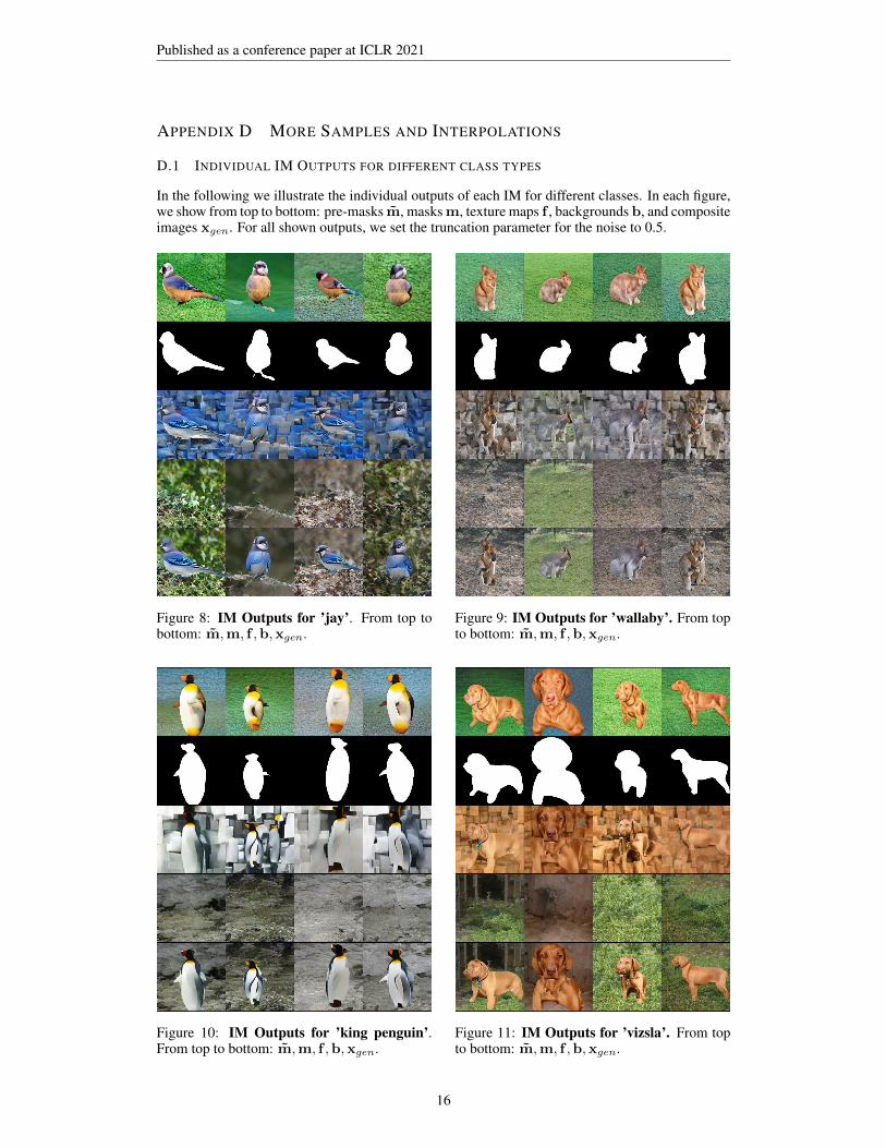
D.1 INDIVIDUAL IM OUTPUTS FOR DIFFERENT CLASS TYPES

In the following we illustrate the individual outputs of each IM for different classes. In each figure,we show from top to bottom: pre-masks m, masks m, texture maps f , backgrounds b, and compositeimages xgen. For all shown outputs, we set the truncation parameter for the noise to 0.5.

Figure 8: IM Outputs for ’jay’. From top tobottom: m,m, f ,b,xgen.

Figure 9: IM Outputs for ’wallaby’. From topto bottom: m,m, f ,b,xgen.

Figure 10: IM Outputs for ’king penguin’.From top to bottom: m,m, f ,b,xgen.

Figure 11: IM Outputs for ’vizsla’. From topto bottom: m,m, f ,b,xgen.

16


Figure 12: IM Outputs for ’barn’. From top tobottom: m,m, f ,b,xgen.

Figure 13: IM Outputs for ’speedboat’. Fromtop to bottom: m,m, f ,b,xgen.

Figure 14: IM Outputs for ’viaduct’. From topto bottom: m,m, f ,b,xgen.

Figure 15: IM Outputs for ’cauliflower’.From top to bottom: m,m, f ,b,xgen.

17


Figure 16: IM Outputs for ’bell pepper’.From top to bottom: m,m, f ,b,xgen.

Figure 17: IM Outputs for ’strawberry’.From top to bottom: m,m, f ,b,xgen.

Figure 18: IM Outputs for ’geyser’. From topto bottom: m,m, f ,b,xgen.

Figure 19: IM Outputs for ’agaric’. From topto bottom: m,m, f ,b,xgen.

18


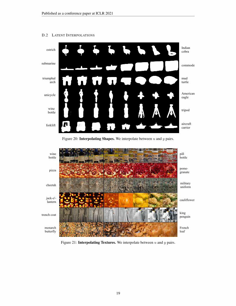
D.2 LATENT INTERPOLATIONS

ostrichIndian cobra

submarine

triumphal arch

unicycle

wine bottle

forklift aircraft carrier

tripod

American eagle

mud turtle

commode

Figure 20: Interpolating Shapes. We interpolate between u and y pairs.

winebottle

pill bottle

pizza

cheetah

jack-o'-lantern

trench coat

monarchbutterfly

French loaf

king penguin

cauliflower

pome-granate

military uniform

Figure 21: Interpolating Textures. We interpolate between u and y pairs.

19


waterouzel

fig

sandbar

axolotl

mushroom

cliff

grey whale coral reef

mud turtle

valley

viaduct

Airedale terrier

Figure 22: Interpolating Backgrounds. We interpolate between u and y pairs.

D.3 MORE COUNTERFACTUAL SAMPLES

Figure 23: MNIST Counterfactuals. From Left to Right: colored, double-colored-, and WildlifeMNIST.

20


Row Column Shape Texture Background

1 1 school bus panda geyser

1 2 hyena dog chello strawberry

1 3 robin lipstick diving

1 4 Indian cobra analog clock green lizard

1 5 race car piggy bank fig

2 1 hyena dog breastplate cock

2 2 German shepherd king penguin bittern

2 3 beaker busby pineapple

2 4 Indian Cobra orange spider web

2 5 teddy beer glass rock crab

3 1 malinois reel viaduct

3 2 ibex upright piano sand bank

3 3 hourglass lemon hornbill

Row Column Shape Texture Background

3 4 offshore rig ambulance breakwater

3 5 mushroom sand viper ostrich

4 1 snowmobile French Loaf Arabian camel

4 2 katamaran cheetah garden spider

4 3 bald eagle strawberry spike

4 4 triumphal arc standard poodle bullfrog

4 5 forklift theater curtain valley

5 1 whine bottle pill bottle alp

5 2 pirate ship trench coat beaver

5 3 submarine race car hay

5 4 wood rabbit jack-o'-lantern water ouzel

5 5 teapot military uniform baseball

Figure 24: ImageNet Counterfactuals. Top: Counterfactual Images. Bottom: ImageNet labels.

21


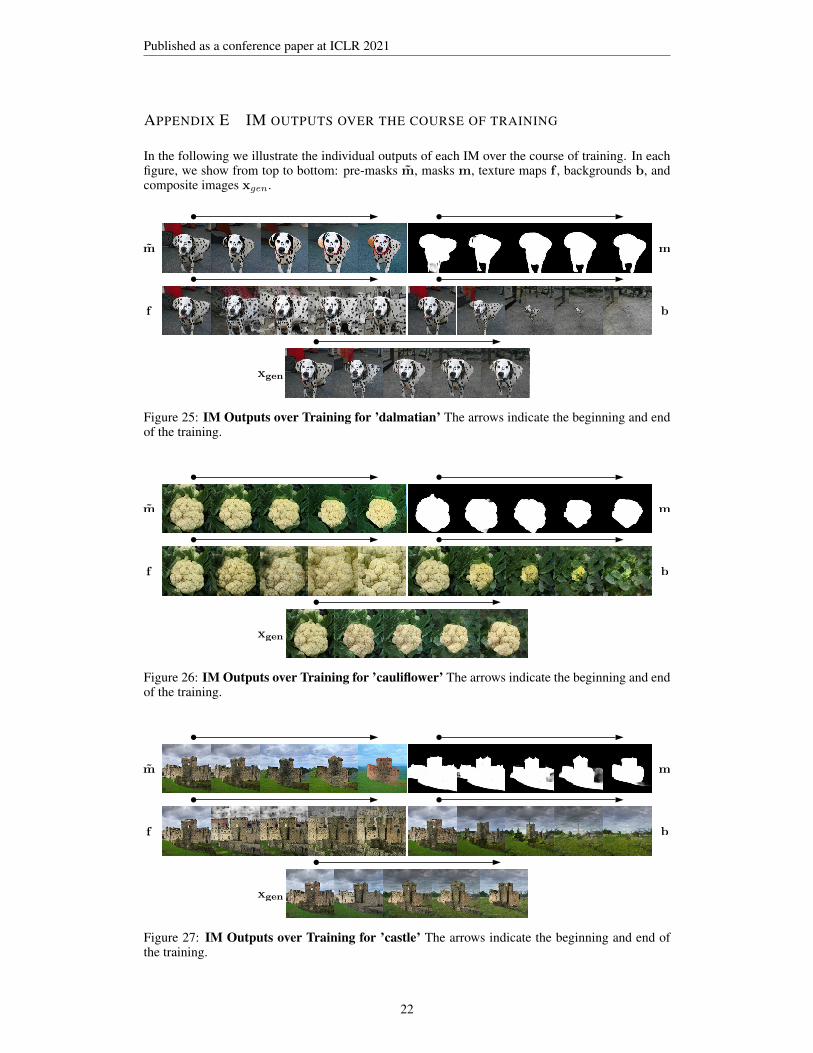
APPENDIX E IM OUTPUTS OVER THE COURSE OF TRAINING

In the following we illustrate the individual outputs of each IM over the course of training. In eachfigure, we show from top to bottom: pre-masks m, masks m, texture maps f , backgrounds b, andcomposite images xgen.

Figure 25: IM Outputs over Training for ’dalmatian’ The arrows indicate the beginning and endof the training.

Figure 26: IM Outputs over Training for ’cauliflower’ The arrows indicate the beginning and endof the training.

Figure 27: IM Outputs over Training for ’castle’ The arrows indicate the beginning and end ofthe training.

22


Figure 28: IM Outputs over Training for ’ringtailed lemur’ The arrows indicate the beginningand end of the training.

Figure 29: IM Outputs over Training for ’mushroom’ The arrows indicate the beginning and endof the training.

23


APPENDIX F FAILURE CASES OF CGN

Figure 30: Texture-Background Entanglement. For relatively small objects, the texture maps canstill show traces of the background. A possible remedy would be to choose the patch size for Ltext

dependent on the relative object size.

Figure 31: Background Residues. Especially for large objects, i.e., where large regions need to bein-painted, there can be faint artifacts visible. For the composite images, this is not a problem as anobject will cover the residue.

Figure 32: Reduced Realism. As evidence by the lower IS, the generated images xgen are generallylower in realism. This reduced realism is due to the constraints that we enforce and the simplifiedcomposition mechanism. A solution might be to add a shallow refinement network after the com-poser.

24


APPENDIX G COLLAPSING MASKS

Figure 33: Masks when disabling different losses. From left to right: the beginning of training,training without Lshape, training without Ltext, training without Lbg , training with all losses. Thethird and fourth columns show the collapse of the masks, as described in section 4.2.

APPENDIX H CGN AUGMENTATION WITH IRM ASSUMPTIONS

We can drop the assumption of a priori knowledge of the causal signal and follow the same assump-tion as IRM: several environments with varying correlations, an invariant signal is considered causal.In the following, we train a CGN on double-colored MNIST. We then generate counterfactual datato train three classifiers:

• Shape classifier (SC): invariant wrt. object color and background color• Object color classifier (OCC): invariant wrt. object shape and background color• Background color classifier (BCC): one invariant wrt. object shape and object color

We can measure their respective performance in the environments used to train IRM. In these envi-ronments, only the shape is stably correlated with the label; the foreground and background colorvary in their degree of correlation. Based on the results in Table 5, we can determine the shape to bethe causal signal as only the test accuracy of SC is stable across environments.

Degree of Correlation Accuracy SC [%] Accuracy OCC [%] Accuracy BCC [%]

90 % 85.05 ± 0.12 58.72 ± 0.67 82.47 ± 0.1395 % 85.08 ± 0.07 62.69 ± 0.58 87.96 ± 0.12100 % 85.14 ± 0.10 65.05 ± 1.32 90.16 ± 0.13

Table 5: Test Accuracy on double-colored MNIST. We report the mean and standard deviationover three random seeds.

25

COUNTERFACTUAL GENERATIVE NETWORKS

Documents

Transcript of COUNTERFACTUAL GENERATIVE NETWORKS