Goldstein S. - The Quantum Formalism and the GRW Formalism (2012)
Upload
matthew-geletaCategory
view
401download
17
The Coulomb Gas Formalism
in Conformal Field Theory
Matthew D. Geleta
Supervisor: David Ridout
A thesis submitted for the degree of
Bachelor of Science with Honours in Physics
College of Physical and Mathematical SciencesResearch School of Physics and Engineering
Department of Theoretical Physics

The Coulomb Gas Formalismin Conformal Field Theory
Author: Matthew D. GeletaSupervisor: David RidoutDepartment: Department of Theoretical PhysicsUniversity: The Australian National UniversityDate of submission: 22 October 2015
Abstract
Conformal field theory is an area of theoretical and mathematical physics that has applicationsin statistical physics, string theory, interacting quantum field theories, and many branches ofmathematics. The Coulomb gas formalism is a celebrated technique in conformal field theorythat provides effective machinery for describing critical phenomena that arise in the scaling limitof certain two-dimensional statistical lattice models.
In this work we develop the Coulomb gas formalism starting from a bosonic string theory.We demonstrate some applications in statistical field theory by constructing minimal modelconformal field theories and relating these to three different critical lattice models, namely theIsing model, the tricritical Ising model, and the Yang-Lee model. We then use the Coulombgas formalism to analytically compute all of the primary three-point constants and primaryoperator-product expansion coefficients for the minimal conformal field theories correspondingto these critical models. We compare Coulomb gas calculations with results obtained usingother standard techniques, namely bosonisation of the free fermion conformal field theory, andthe conformal bootstrap in Liouville theory. We also compare Coulomb gas calculations with anon-standard technique of our own construction, based on the monodromy theory of Fuchsiandifferential equations. All comparisons are consistent with the Coulomb gas calculations.
The main original contribution of this work is to conjecture and verify a connection betweenthe Coulomb gas formalism and the monodromy theory of certain Fuchsian differential equations.The success of the verification suggests an opportunity to extend Coulomb gas methods beyondconformal field theory and, conversely, for greater application of the monodromy theory ofdifferential equations in conformal field theory.
i

ii
Declaration
This thesis is an account of research undertaken between February 2015 and October 2015 atthe Department of Theoretical Physics, Research School of Physics and Engineering, College ofPhysical and Mathematical Sciences, The Australian National University, Canberra, Australia.
Except where acknowledged in the customary manner, the material presented in this thesisis, to the best of my knowledge, original and has not been submitted in whole or in part for adegree at any university.
Matthew D. Geleta
22 October 2015

Dedicated to Peter and Sharon
iii

Acknowledgements
Foremost, thank you David. Your vast knowledge, admirable work ethic, and masterful lecturenotes [114] are inspiring. I have learned more from you this year than I could have expected to.Thank you for your patience and for understanding my misunderstandings... there were so manymisunderstandings to understand, yet you somehow understood. I sincerely hope that we worktogether in the future.
Next up is Simon. Thank you. I got stuck many times this year and often you pointed me inthe right direction, providing the insight and expertise needed to move forward. I have learnedso much from you, and not only from your lectures [131]. The rumours are true — you areindeed one very smart chap. I would have made much less progress were it not for your frequentassistance.
Tian, thank you for your empathy, positivity and encouragement, and for letting me learnfrom your own honours thesis [90].
Thank you Peter and Sharon for supporting me in every conceivable way, despite the factthat all I offered in return was a barrage of detailed complaints and a deluge of... let us go withcoffee. Cowboys, I am told, do not cry. You mean more to me than anything in this world. Nohyperbole attached.
Thank you Lottie for putting up with my brooding and perpetual mathematical ramblings.Seeing you was a highlight of every day.
To my honours friends, congratulations! “You can’t really get more thankful than I am rightnow.” To all remaining friends and family whom I have shamefully neglected, both in real lifeand in this acknowledgements section, I apologise and thank you for understanding. I shall makeit up to every one of you.
Finally, I thank the Dunbar Physics Honours Scholarship committee. Had I not receivedsuch generous support, this year would not have happened. I am immensely grateful for theopportunity it afforded me, and can only hope that the quality of my thesis reflects my gratitude.
References in this thesis were managed with [79], and illustrations were made with [73].
iv

Contents
Abstract i
Declaration ii
Acknowledgements v
Introduction 1
1 Representing Symmetry 5
1.1 Lie groups and Lie algebras . . . . . . . . . . . . . . . . . . . . . . . . . . . . . . 5
1.2 Representations . . . . . . . . . . . . . . . . . . . . . . . . . . . . . . . . . . . . . 7
1.2.1 Triangular decomposition . . . . . . . . . . . . . . . . . . . . . . . . . . . 8
1.2.2 Highest weight modules . . . . . . . . . . . . . . . . . . . . . . . . . . . . 8
1.2.3 Universal enveloping algebra . . . . . . . . . . . . . . . . . . . . . . . . . 9
1.3 Fock spaces . . . . . . . . . . . . . . . . . . . . . . . . . . . . . . . . . . . . . . . 9
1.4 Scalar products . . . . . . . . . . . . . . . . . . . . . . . . . . . . . . . . . . . . . 9
1.5 Partition basis . . . . . . . . . . . . . . . . . . . . . . . . . . . . . . . . . . . . . 10
2 Conformal Invariance 12
2.1 Conformal transformations . . . . . . . . . . . . . . . . . . . . . . . . . . . . . . 12
2.1.1 Global transformations . . . . . . . . . . . . . . . . . . . . . . . . . . . . . 13
2.1.2 Conformal group . . . . . . . . . . . . . . . . . . . . . . . . . . . . . . . . 14
2.1.3 Infinitesimal transformations . . . . . . . . . . . . . . . . . . . . . . . . . 14
2.2 Conformal invariance in two dimensions . . . . . . . . . . . . . . . . . . . . . . . 15
2.2.1 The Mobius group . . . . . . . . . . . . . . . . . . . . . . . . . . . . . . . 16
2.2.2 The classical conformal algebra . . . . . . . . . . . . . . . . . . . . . . . . 17
3 Fundamentals and Techniques 19
3.1 Fields and states . . . . . . . . . . . . . . . . . . . . . . . . . . . . . . . . . . . . 19
3.1.1 Fields . . . . . . . . . . . . . . . . . . . . . . . . . . . . . . . . . . . . . . 19
3.1.2 States . . . . . . . . . . . . . . . . . . . . . . . . . . . . . . . . . . . . . . 20
3.1.3 The state-field correspondence . . . . . . . . . . . . . . . . . . . . . . . . 20
3.2 Operator-product expansions (OPEs) . . . . . . . . . . . . . . . . . . . . . . . . . 21
3.2.1 Radial ordering . . . . . . . . . . . . . . . . . . . . . . . . . . . . . . . . . 22
3.3 The energy-momentum tensor and the Virasoro algebra . . . . . . . . . . . . . . 22
3.4 Correlation functions . . . . . . . . . . . . . . . . . . . . . . . . . . . . . . . . . . 23
3.4.1 Chiral and physical correlators . . . . . . . . . . . . . . . . . . . . . . . . 23
v

CONTENTS vi
3.5 The conformal Ward identities . . . . . . . . . . . . . . . . . . . . . . . . . . . . 24
3.5.1 Consequences of the Ward identities . . . . . . . . . . . . . . . . . . . . . 25
3.5.2 Unphysical fields . . . . . . . . . . . . . . . . . . . . . . . . . . . . . . . . 26
3.5.3 Operator-product expansions and correlation functions . . . . . . . . . . . 27
3.6 The main objective of this thesis . . . . . . . . . . . . . . . . . . . . . . . . . . . 27
3.7 Fundamental techniques . . . . . . . . . . . . . . . . . . . . . . . . . . . . . . . . 27
3.7.1 Commutation relations from generating functions . . . . . . . . . . . . . . 27
3.7.2 Defining OPEs . . . . . . . . . . . . . . . . . . . . . . . . . . . . . . . . . 29
3.7.3 Descendent correlators from primary correlators . . . . . . . . . . . . . . 29
4 Vertex Operators and the Free Boson 32
4.1 The classical free boson . . . . . . . . . . . . . . . . . . . . . . . . . . . . . . . . 32
4.1.1 Wick rotation . . . . . . . . . . . . . . . . . . . . . . . . . . . . . . . . . . 33
4.1.2 Conformal invariance . . . . . . . . . . . . . . . . . . . . . . . . . . . . . . 33
4.2 The quantum free boson . . . . . . . . . . . . . . . . . . . . . . . . . . . . . . . . 34
4.2.1 The Heisenberg algebra . . . . . . . . . . . . . . . . . . . . . . . . . . . . 34
4.2.2 The Virasoro algebra and the energy-momentum tensor . . . . . . . . . . 35
4.3 The state-field correspondence . . . . . . . . . . . . . . . . . . . . . . . . . . . . 37
4.3.1 Virasoro modules in Fock spaces . . . . . . . . . . . . . . . . . . . . . . . 37
4.4 Scalar products . . . . . . . . . . . . . . . . . . . . . . . . . . . . . . . . . . . . . 38
4.5 Wick’s theorem for bosons . . . . . . . . . . . . . . . . . . . . . . . . . . . . . . . 38
4.6 Vertex operators . . . . . . . . . . . . . . . . . . . . . . . . . . . . . . . . . . . . 39
4.6.1 Extending the Heisenberg algebra . . . . . . . . . . . . . . . . . . . . . . 39
4.6.2 Vertex operators . . . . . . . . . . . . . . . . . . . . . . . . . . . . . . . . 41
4.6.3 Vertex operators in correlation functions . . . . . . . . . . . . . . . . . . . 41
4.6.4 Solving the free boson . . . . . . . . . . . . . . . . . . . . . . . . . . . . . 42
4.7 Physical correlation functions . . . . . . . . . . . . . . . . . . . . . . . . . . . . . 42
5 Virasoro Representations and the Minimal Models 45
5.1 Verma modules . . . . . . . . . . . . . . . . . . . . . . . . . . . . . . . . . . . . . 45
5.1.1 Scalar product . . . . . . . . . . . . . . . . . . . . . . . . . . . . . . . . . 46
5.2 Singular vectors . . . . . . . . . . . . . . . . . . . . . . . . . . . . . . . . . . . . . 46
5.2.1 Unphysical states . . . . . . . . . . . . . . . . . . . . . . . . . . . . . . . . 47
5.3 Finding singular vectors . . . . . . . . . . . . . . . . . . . . . . . . . . . . . . . . 48
5.3.1 The Kac determinant . . . . . . . . . . . . . . . . . . . . . . . . . . . . . 49
5.4 Singular fields in correlation functions . . . . . . . . . . . . . . . . . . . . . . . . 50
5.4.1 Fusion rules . . . . . . . . . . . . . . . . . . . . . . . . . . . . . . . . . . . 51
5.5 The minimal models . . . . . . . . . . . . . . . . . . . . . . . . . . . . . . . . . . 54
5.5.1 Physical relevance of minimal model theories . . . . . . . . . . . . . . . . 54
5.6 Example: the Ising model and M(3, 4) . . . . . . . . . . . . . . . . . . . . . . . . 55
5.6.1 The Ising model . . . . . . . . . . . . . . . . . . . . . . . . . . . . . . . . 55
5.6.2 The minimal model M(3, 4) . . . . . . . . . . . . . . . . . . . . . . . . . . 55
6 Bosons, Fermions, and the Ising Model 57
6.1 The free fermion . . . . . . . . . . . . . . . . . . . . . . . . . . . . . . . . . . . . 57

CONTENTS vii
6.1.1 Statistical mechanics . . . . . . . . . . . . . . . . . . . . . . . . . . . . . . 60
6.2 Bosonisation of the free fermion . . . . . . . . . . . . . . . . . . . . . . . . . . . . 60
6.2.1 Tensor products of representations . . . . . . . . . . . . . . . . . . . . . . 60
6.3 Fermionisation of the free boson . . . . . . . . . . . . . . . . . . . . . . . . . . . 62
6.4 Solving the Ising model . . . . . . . . . . . . . . . . . . . . . . . . . . . . . . . . 62
6.4.1 Ising model correlation functions . . . . . . . . . . . . . . . . . . . . . . . 62
6.4.2 Ising three-point constants by bosonisation . . . . . . . . . . . . . . . . . 63
6.A Appendix: Fermionic version of Wick’s theorem . . . . . . . . . . . . . . . . . . . 67
7 Differential Equations and Monodromy 68
7.1 Four-point functions . . . . . . . . . . . . . . . . . . . . . . . . . . . . . . . . . . 68
7.2 The hypergeometric class . . . . . . . . . . . . . . . . . . . . . . . . . . . . . . . 69
7.2.1 Hypergeometric functions . . . . . . . . . . . . . . . . . . . . . . . . . . . 70
7.3 Monodromy and the two-point connection problem . . . . . . . . . . . . . . . . . 71
7.3.1 Monodromy . . . . . . . . . . . . . . . . . . . . . . . . . . . . . . . . . . . 71
7.3.2 The two-point connection problem . . . . . . . . . . . . . . . . . . . . . . 72
7.3.3 The anti-holomorphic sector . . . . . . . . . . . . . . . . . . . . . . . . . . 75
7.A Appendix: From PDE to ODE . . . . . . . . . . . . . . . . . . . . . . . . . . . . 76
7.B Appendix: Connection coefficients . . . . . . . . . . . . . . . . . . . . . . . . . . 77
7.C Appendix: Convergence information . . . . . . . . . . . . . . . . . . . . . . . . . 78
8 The Coulomb Gas Formalism 79
8.1 Modifying the free boson . . . . . . . . . . . . . . . . . . . . . . . . . . . . . . . . 79
8.2 Screening fields . . . . . . . . . . . . . . . . . . . . . . . . . . . . . . . . . . . . . 80
8.3 Realising the minimal models . . . . . . . . . . . . . . . . . . . . . . . . . . . . . 81
8.4 Neutrality . . . . . . . . . . . . . . . . . . . . . . . . . . . . . . . . . . . . . . . . 82
8.4.1 Neutrality on the level of states . . . . . . . . . . . . . . . . . . . . . . . . 82
8.4.2 Neutrality for correlation functions . . . . . . . . . . . . . . . . . . . . . . 83
8.4.3 Neutrality and conservation of momentum . . . . . . . . . . . . . . . . . . 83
8.4.4 Neutrality and screening operators . . . . . . . . . . . . . . . . . . . . . . 83
8.5 Computing four-point functions . . . . . . . . . . . . . . . . . . . . . . . . . . . . 86
8.5.1 Monodromy invariance . . . . . . . . . . . . . . . . . . . . . . . . . . . . . 87
8.5.2 Contour manipulations . . . . . . . . . . . . . . . . . . . . . . . . . . . . . 89
8.5.3 Computing OPE-coefficients . . . . . . . . . . . . . . . . . . . . . . . . . . 91
8.6 Solving statistical models . . . . . . . . . . . . . . . . . . . . . . . . . . . . . . . 94
8.6.1 The Ising model . . . . . . . . . . . . . . . . . . . . . . . . . . . . . . . . 94
8.6.2 The Yang-Lee model . . . . . . . . . . . . . . . . . . . . . . . . . . . . . . 94
8.7 The general procedure . . . . . . . . . . . . . . . . . . . . . . . . . . . . . . . . . 95
8.7.1 The tricritical Ising model . . . . . . . . . . . . . . . . . . . . . . . . . . . 96
8.8 Relationship to the connection problem . . . . . . . . . . . . . . . . . . . . . . . 97
8.A Appendix: Coulomb gas energy-momentum tensor . . . . . . . . . . . . . . . . . 100
Conclusion 101

Introduction
“Seek first to understand...”
Statistical mechanics and critical phenomena, string theory and quantum gravity, monstrousmoonshine and modular forms, supersymmetry, condensed matter physics, number theory,representation theory, quantum groups... this is the realm of conformal field theory.
The 1970s and early 1980s were particularly prosperous times for fundamental physics, rifewith influential research such as the work of Polyakov [106–109] and Witten [1,128–130]. Thefoundations had been laid for another conceptual leap, and this leap was made in 1984 with [9],which made a simple observation — two-dimensional quantum field theories with a particulartype of symmetry have infinite-dimensional symmetry algebras. The symmetry in question isconformal symmetry and its consequences are profound. This was the birth of conformal fieldtheory as it is known today.
Conformal field theory
A conformal field theory is a two-dimensional quantum field theory with conformal symmetry.
The subsequent years saw conformal field theory ripen into a rich and mature area oftheoretical physics. There were a number of drivers for progress. At the time, field theories wereplaying an increasingly prominent role in statistical physics [88], and here conformal field theoriesfound great application. They were found to describe and classify critical phenomena [122],such as the onset of superconductivity in metals [68] and the spontaneous magnetisation offerromagnets [78]. On the other hand there were its applications in string theory and the searchfor a quantum theory of gravity [29, 32, 110]. In later years conformal field theory even foundapplication in describing the entropy of black holes [23,69]. Moreover, conformal field theory isresponsible for great developments in mathematics, such as the birth of vertex algebras and theirrole in proving [17] the infamous monstrous moonshine conjectures of Conway and Norton [26],for which Borcherds received his 1998 Fields Medal [62]. Conformal field theory still plays aleading role in each of these fields today. It is a true gem of theoretical and mathematical physics.
Our focus will be on applications to statistical physics. In particular, we construct a class ofconformal field theories called the minimal models. These were conceived in [9], and describethe critical behaviour of many of the famous two-dimensional statistical models in their scalinglimits [14] — the Ising model [22] and its variations [56, 86], the Potts models [8, 37], and theYang-Lee model [21], to name a few. Theoretical physicists know all too well how difficult it canbe to deal with these models analytically, a good example being Onsager’s solution to the Isingmodel [100]. Often one defers to approximate numerical methods [11, 19]. We will not — one ofthe most attractive aspects of conformal field theory is that the problems it deals with are, inprinciple, exactly solvable.
1

CONTENTS 2
Statistical field theory
The scaling limit of a statistical lattice model is the limit in which the lattice spacing is taken tozero in an appropriate way (for example by block spin renormalisation [81]) so that particularlattice observables are described by a statistical field theory — these observables are scalingfields. It is here that critical phase transitions arise — this is the domain of the renormalisationgroup and conformal field theory [12,25].
Phase transitions are a treasured phenomenon in statistical physics. In the thermodynamiclimit, a statistical phase transition is a discontinuous change in a thermodynamic quantity assome parameter is varied continuously across a critical value. Some phase transitions, such asthe melting of ice, are associated with a latent heat. Here a finite amount of energy must besupplied for the phase transition to occur, and during this process the macroscopic properties donot change. These are the first-order phase transitions, so called because the free energy has adiscontinuity in one of its first derivatives. There are also critical phenomena [91], or second-orderphase transitions — here there is no latent heat and the first derivatives of the free energy remaincontinuous, although there is a discontinuity in one of the second derivatives. An example is thespontaneous onset of magnetisation in a ferromagnet surrounded by negligible external magneticfield, which occurs when the temperature is lowered past the Curie temperature. It is at thesecritical points that conformal invariance arises — Polyakov had already demonstrated this asearly as 1970 [105], but it took over a decade for the consequences to become widely appreciated.
The thermodynamic properties of a generic statistical lattice model are described by a set ofobservables, for example the spin or energy density at each lattice site in a model of a ferromagnet.The values taken by observables at different locations (and times) on the lattice are usually notindependent, and their inter-dependence is quantified through correlation functions — these areparticular ensemble averages over lattice configurations. The common lore of critical phenomenais, roughly speaking, that information about the state of one lattice site is propagated to othersvia inter-site interactions, which causes the observables at each site to become correlated. Athigh temperatures, thermal fluctuations dominate over interactions between lattice sites. Whenthe distance Rij between two lattice sites i and j is much greater than some characteristiclength scale ξA,B for two observables A and B, the correlation between the observables decaysexponentially with increasing distance:
〈AiBj〉 ∼ e−Rij/ξA,B , Rij ξA,B. (1)
The characteristic length scale ξA,B, or correlation length, decreases in the limit of high temper-atures. At a critical point the correlation length diverges, the theory becomes scale-invariant,and the correlation functions decay not exponentially, but rather according to a power law.Remarkably, under a few reasonable assumptions [104], a locally scale-invariant theory in twodimensions exhibits a far stronger symmetry — conformal symmetry. Strong symmetry severelyconstrains the possible behaviour of the system, and opens up a range of mathematical tools fortheoretical inquiry.
The Ising model
The most famous example of a statistical lattice model is the Ising model [93] — an ostensiblyinnocuous lattice model that exhibits surprisingly non-trivial behaviour. The Ising modeldescribes the behaviour of a simple ferromagnet and, in the thermodynamic limit, exhibitsspontaneous magnetisation as the temperature is varied across a critical value. The modelpossesses observables such as the spin density σi and energy density εj , local to the lattice sitesi and j respectively. At the critical temperature, the Ising model correlation functions decay

CONTENTS 3
according to the power laws [45]
〈σiσj〉 ∼1
Rd−2+ηij
∼ 1
R2∆σij
, 〈εiεj〉 ∼1
R2(d−1/ν)ij
∼ 1
R2∆εij
, (2)
where d is the number of dimensions of the lattice, η, ν ∈ R are called critical exponents, and∆σ,∆ε ∈ R are called scaling dimensions of the observables σ and ε. These values characteriseand classify the behaviour of the model at the critical point. For some lattice models, like theIsing model, the critical exponents and scaling dimensions are known exactly [100]; for othersthey are not, and are usually estimated numerically [11,19].
One of the great successes of conformal field theory is that it can be used to analyticallycompute critical exponents and scaling dimensions permitted by conformal symmetry in two-dimensional field theories, such as the scaling limit of a critical lattice model, thereby providing aclassification scheme for critical phenomena [55]. Critical exponents are determined by the natureof the interactions between lattice sites, and critical lattice models can be put into universalityclasses [20] based on their critical exponents. For example, in chapter 5 we relate the Ising model(and all models in the same universality class) to a conformal field theory called M(3, 4), whichpredicts the aforementioned critical exponents, and we use it to compute correlation functionsexplicitly.
The tricritical Ising model
Some fascinating phenomena emerge when the conventional Ising model is modified by annealing,allowing lattice sites to be vacant (equivalently, permitting spin values of zero). There arises atricritical point at which three different phases can coexist [87]. At this critical point the scalingfields are described by another of the conformal field theories that we will be constructing — aminimal model called M(4, 5) [86]. Conformal field theory provides tools sufficient to determinethe critical exponents and scaling dimensions of the scaling fields in this model, and to computecorrelation functions analytically. On top of its importance in statistical physics, one of the mostinteresting features ofM(4, 5) is that it is endowed with supersymmetry — the conformal algebrathat characterises M(4, 5) can be extended to a superconformal algebra [56]. Hence not only isM(4, 5) of interest in statistical physics, but it is a playground for studying the mathematicsof supersymmetry, which plays a distinguished role in string theory, and might one day be astandard component of fundamental physics.
The Coulomb gas formalism
A powerful aspect of conformal field theory is that its string theory and statistical field theorydivisions walk side by side — many statistical field theoretical problems can be translated intostring theoretical language and solved with reduced effort, and vice versa. The key insight is torecognise the relationship between the two.
With this idea in mind, an overarching goal of this thesis is to construct and then use sometools from string theory to find critical exponents and compute correlation functions of observablesin critical statistical models. In the series of papers [34–36], a technique was introduced whichturns out to be perfectly suited to our aims. This is the Coulomb gas formalism. Deriving andthen using this technique is the end goal of this work.
Thesis outline
Chapters 1 and 2 cover preliminaries. If a quantum field theory exhibits symmetry, then muchof its behaviour can be deduced by studying the representation theory of its symmetry algebra(or group), and this is where we commence in chapter 1. In chapter 2 we review conformal

CONTENTS 4
symmetry, and derive an infinite-dimensional symmetry algebra of conformal transformations.The representation theory of this symmetry algebra allows us to quantify the constraints ofconformal symmetry, which we use later to solve problems in statistical physics. Chapter 3deals with the fundamental principles of conformal field theory, and here we develop essentialmathematical techniques that will guide us through subsequent chapters. In chapter 4 we putour background knowledge to good use in a first encounter with a true conformal field theory
— a massless scalar free field theory called the free boson. This is a conformal field theory thatfeatures prominently in string theory. The free boson is used to construct vertex operators,which are essential in subsequent chapters. In chapter 5 we isolate the consequences of quantumconformal symmetry by examining the representation theory of the conformal algebra. Here weconstruct the minimal models, and discuss some of their salient features in relation to statisticalfield theory. Chapter 6 introduces the free fermion conformal field theory, another examplefrom string theory. Here the vertex operators from chapter 4 and the representation theoryof chapter 5 are combined with the free fermion theory, and used to solve the critical Isingmodel. Chapter 7 is the penultimate chapter, and here we take a slight detour from the algebraicapproach of the previous chapters to consider some differential equations. Conformal symmetryimposes constraints on quantum systems, and these manifest as partial differential equationssatisfied by correlation functions — with a few manipulations and some physical consistencyconditions, we are able to transform these into ordinary differential equations and solve them.
Finally in chapter 8 everything is brought together. In the spirit of conformal field theory, theaim is to connect up knowledge from diverse areas; in particular we point out a close relationshipbetween the Coulomb gas formalism and the differential equations of chapters 5 and 7. In thisfinal chapter we draw on content from all of the previous chapters, culminating in the solution ofthree different statistical models.

Chapter 1
Representing Symmetry
The beauty of physics and mathematics stems in no small part from symmetry. Conformalfield theory as applied to relativistic quantum field theory is essentially the study of the highlynon-trivial consequences of a particular type of symmetry — conformal symmetry. To appreciatethe power of conformal symmetry and to make the notion quantitative, we need some tools fromthe theory of Lie algebras1 and their representations, and this is where we commence our journey.
This chapter covers mathematical preliminaries that will be used in subsequent chapters.Readers familiar with Lie algebras and Lie algebra modules may wish to skip this chapter in afirst reading, and refer to it as necessary.
1.1 Lie groups and Lie algebras
Consider the equation for a circle of radius r ∈ R>0 centred at the origin of R2:
x2 + y2 = r2. (1.1)
The circle is the collection of points (x, y) ∈ R2 which satisfy eq. (1.1). The plane can be rotated:(x′
y′
)=
(cos θ − sin θsin θ cos θ
)(xy
), (1.2)
and the new point (x′, y′) solves eq. (1.1) whenever (x, y) does, thus rotations of the plane aresaid to be a symmetry for the circle.2 The collection of all 2× 2 rotation matrices forms a Liegroup.
The symmetries of a quantum system are also encoded by the action of a symmetry group(or algebra). A group is a set G equipped with a binary operation : G×G→ G which satisfies
• Associativity: (a b) c = a (b c) for all a, b, c ∈ G.
• Identity: There is an element 1 ∈ G which satisfies a 1 = 1 a = a for every a ∈ G.
• Invertibility: For every a ∈ G there is an inverse element denoted by a−1 which satisfiesa a−1 = a−1 a = 1.
It follows from the group axioms that the identity element is unique, that each a ∈ G has a uniqueinverse, and that (a−1)−1 = a. A Lie group is a group that is also a differentiable manifoldwith the property that the group operations of multiplication and inversion are differentiable
1“Lie” is pronounced “Lee”, named after Sophus Lie.2This example is borrowed from [95].
5

CHAPTER 1. REPRESENTING SYMMETRY 6
maps. If a subset of a group also satisfies the group axioms, and contains the same identityelement as the group, then this subset is called a subgroup.
Example: General linear groupThe set of real n× n invertible matrices, together with matrix multiplication and inversion asthe group operations, is called the real general linear group of degree n, denoted by GL(n,R). Ifwe allow complex matrices, then we have the complex general linear group of degree n, denotedby GL(n,C). The group GL(n,R) (respectively GL(n,C)) is a Lie group because the matricescan be considered to be points on an n× n-dimensional real (respectively complex) differentiablemanifold, and because matrix multiplication and inversion are both differentiable with respect tothe matrix coefficients.
Example: Special linear groupThe set of real (respectively complex) n× n matrices with unit determinant is called the real(respectively complex) special linear group, denoted by SL(n,R) (respectively SL(n,C)). It is asubgroup of the general linear group because any product of matrices with unit determinant isalso a matrix with unit determinant. It is a Lie group.
Closely related to Lie groups are Lie algebras, which are infinitesimal linearisations of Liegroups — see [57, Ch. 9]. A Lie algebra is a vector space g equipped with a bilinear pairing[·, ·] : g× g→ g called the Lie bracket. For all x, y, z ∈ g, the Lie bracket satisfies
• Antisymmetry: [x, y] = −[y, x].
• Jacobi identity: [[x, y], z] + [[y, z], x] + [[z, x], y] = 0.
Note that in general a Lie algebra is neither an associative nor a commutative algebra. If x, y ∈ gsatisfy [x, y] = 0, then x and y are said to commute, and if all elements of a Lie algebracommute, then the algebra is called abelian. The set of elements that commute with the wholealgebra is called the centre of the algebra, denoted by Z(g). A subalgebra of a Lie algebra isa vector subspace that is closed under the Lie bracket. The centre of a Lie algebra is always asubalgebra.
Example: General linear Lie algebraIf a Lie algebra is over the field R then it is a real Lie algebra. The vector space of n×n matriceswith real coefficients becomes a real Lie algebra if we take the commutator of matrices to bethe Lie bracket. This algebra is called the real general linear Lie algebra of degree n, and isdenoted by gl(n,R). In this work we shall always take the field to be C, in which case we have acomplex Lie algebra. The analogous complex general linear Lie algebra of degree n is denoted bygl(n,C).
Example: Virasoro algebraThe most important Lie algebra in conformal field theory is the Virasoro algebra — an infinite-dimensional (complex) Lie algebra Vir :=
⊕n∈ZCLn ⊕ CC with Lie bracket:3
[Ln, Lm] = (n−m)Ln+m +C
12n(n2 − 1)δn,−m, [Lm, C] = 0. (1.3)
The centre is Z(Vir) = CC. The Virasoro algebra is contained in the symmetry algebra ofevery two-dimensional conformal field theory. It is obtained from another algebra called theWitt algebra, which arises when studying conformal transformations in a classical setting (see
3For readers unfamiliar with this notation, note that for v an element of a vector space over a field F, thesymbol Fv denotes the one-dimensional vector space spanned by v.
CHAPTER 1. REPRESENTING SYMMETRY 7
section 2.2.2).4 The Virasoro algebra is obtained from the Witt algebra by appending to it theelement C. This process is called a central extension [57, Ch. 12]. The coefficient 1/12 multiplyingC in eq. (1.3) is merely conventional and can be set to any complex number by renormalisingC, but apart from this factor the choice of Virasoro commutation relations is the only possibleway to centrally extend the Witt algebra while satisfying the Lie algebra axioms [117, Ch. 5.3].5
Physically, the central extension occurs naturally when quantising a classical conformal fieldtheory (see section 3.3).
Example: Heisenberg algebraThe Heisenberg algebra is an infinite-dimensional Lie algebra H :=
⊕n∈ZCan ⊕ Ck with Lie
bracket:[an, am] = nδn,−mk, [an, k] = 0. (1.4)
The centre is Z(H) = Ca0⊕Ck. The Heisenberg algebra appears remarkably often in many areasof physics. For example, it describes an infinite number of independent harmonic oscillators
— [57, Ch. 2.5]. It is important for us because it can be used to construct the Virasoro algebra.In chapter 4 we will encounter the Heisenberg algebra in the context of string theory, and inchapters 6 and 8 we will use it to solve statistical field theory problems.
1.2 Representations
For modelling the symmetries of a quantum system, it will be convenient to consider the symmetryLie algebra not in abstract form as merely a vector space with a Lie bracket, but rather as acollection of linear operators acting on the quantum state space.
For a vector space V , the collection of linear maps from V to itself is a vector space denotedby EndV . Such maps are called endomorphisms of V . Linear maps can be composed, andcomposition is associative, making EndV into an associative algebra. Any associative algebra canbe turned into a Lie algebra by taking the commutator with respect to the associative productto be the Lie bracket. In this way, EndV becomes a Lie algebra denoted by gl(V ).
A representation of a Lie algebra g on a vector space V is a linear map ρ : g→ gl(V ) thatreplaces Lie brackets by commutators:
ρ([x, y]) = [ρ(x), ρ(y)] = ρ(x)ρ(y)− ρ(y)ρ(x). (1.5)
for all x, y ∈ g. The map ρ is called the representation, and the vector space V is called therepresentation space. The dimension of the representation is the dimension of V , which may beinfinite. A representation of g together with a representation space V is called a g-module. Forx ∈ g and |v〉 ∈ V it is common practice to write x |v〉 instead of ρ(x) |v〉, leaving the map ρimplicit, so that the Lie bracket takes the form of a commutator bracket:
[x, y] |v〉 = x(y |v〉)− y(x |v〉). (1.6)
Since the existence of a representation implies the existence of a representation space, we shall usethe terms “representation” and “module” interchangeably — the former term is more commonin the physics literature, and the latter is more common in the mathematics literature.
A subspace of V that is closed under the action of g is called a submodule. Every g-moduleV has itself and the zero module 0 as submodules. If V has another submodule, then V issaid to be reducible, otherwise it is irreducible. A submodule of V is called proper if it isnot equal to V itself. A submodule of V is called maximal if it is a proper submodule of V thatis not properly contained in another proper submodule of V .
4The Witt algebra is the (complexification of) the Lie algebra of polynomial vector fields on the circle [124].5The Virasoro algebra is the unique non-trivial central extension of the Witt algebra [64]. There is no complex
“Virasoro group” that has the Virasoro algebra as its Lie algebra [117, Thm. 5.4].

CHAPTER 1. REPRESENTING SYMMETRY 8
1.2.1 Triangular decomposition
Some Lie algebras admit a special decomposition into a direct sum of three subalgebrasg = gc ⊕ g0 ⊕ ga. This is called a triangular decomposition if the following axioms aresatisfied [57, Ch. 13.11]:
• For x ∈ gc and y ∈ g0, the bracket [x, y] is in gc.
• For x ∈ ga and y ∈ g0, the bracket [x, y] is in ga.
• g0 is abelian. That is, [x, y] = 0 for all x, y ∈ g0.
• There is an adjoint map.
We define an adjoint map to be a C-linear map † : g → g that is its own inverse and is aone-to-one pairing between ga and gc, and that maps g0 to g0, and reverses the order of the Liebracket: [x, y]† = [y†, x†].6
Triangular decompositions are very common in physics, although seldom formally defined —the elements of gc are called creation operators, those in ga are called annihilation operators,and those in g0 are called zero modes, which accounts for the choice of subscripts. In Lie theory,the subalgebra g0 is called the Cartan subalgebra.7 It is the Cartan subalgebra that containsthe quantum observables.8
Example: General linear Lie algebraConsider the general linear Lie algebra gl(n,C) of n × n complex matrices. If we define thecreation operators gc, annihilation operators ga, and zero modes g0 to be the upper-triangular,lower-triangular, and diagonal matrices respectively, and define the adjoint map to be matrixtransposition, then gl(n,C) = gc ⊕ g0 ⊕ ga is a triangular decomposition.
1.2.2 Highest weight modules
A very important example of a g-module is a highest weight module, which can be constructed forany Lie algebra that admits a triangular decomposition. Highest weight modules arise naturallyin quantum theories — they combine the notion of quantised energy with the requirement thatthe energy of a quantum system be bounded from below. A highest weight module is constructedfrom a vector |v〉 called the vacuum vector, or highest weight vector, in the following way.
Define |v〉 to be a simultaneous eigenvector of each element x in the Cartan subalgebra, andto be annihilated by every annihilation operator. The vector space formed by acting on |v〉 withall finite linear combinations of products9 of a finite number of creation operators is called ahighest weight g-module.
Every g-module constructed by acting on a highest weight vector with creation operators iscalled a highest weight module. One can modify highest weight modules by taking quotientsby submodules (chapter 5). A highest weight module with no modifications is called a Vermamodule, which is in a sense the largest and most general type of highest weight module.
6Adjoint maps are often defined differently in other areas of physics. For example, instead of C-linear theadjoint map is often defined to be Hermitian, so that for B ∈ C and x ∈ g one has (Bx)† = B∗(x)†. The adjointmap is also sometimes defined to be anti-self-inverse. In conformal field theory we use a self-inverse linear adjointmerely for mathematical convenience.
7Technically g0 is the Cartan subalgebra only if g is semi-simple.8In quantum theories that take the adjoint map to be Hermitian, the zero modes that are self-adjoint are the
quantum observables — they necessarily have real eigenvalues. When using a C-linear adjoint map, self-adjointoperators can have complex eigenvalues.
9Products of Lie algebra elements are in the sense explained in section 1.2.3.
CHAPTER 1. REPRESENTING SYMMETRY 9
1.2.3 Universal enveloping algebra
We have seen that any associative algebra can be used to construct a Lie algebra by taking thecommutator with respect to the associative product to be the Lie bracket. Alternatively, startingfrom a Lie algebra g, one may wish to construct an associative algebra that contains g as asubspace and for which the commutator on this subspace reproduces the Lie bracket on g. Foreach Lie algebra g that we shall deal with there is a canonical way to construct such an algebra —see [57, Ch. 14.1]. This algebra is denoted by U(g), and is called the universal enveloping algebraof g. We mention this only for clarity — the only “multiplication” operation defined on a Liealgebra is the Lie bracket, so when we write products of Lie algebra elements, really they areelements of U(g). With this notation the highest weight g-module defined in section 1.2.2 can bewritten succinctly as U(gc) |v〉, which is the same vector space as U(g) |v〉.
To appreciate how this construction works, let us turn to an example very well known in thephysics literature — Fock spaces.
1.3 Fock spaces
Fock spaces are good examples of physically relevant highest weight modules, and play afundamental role in constructing the conformal field theories of chapters 4, 6 and 8. Fock spacesare highest weight representations for the Heisenberg algebra.
The Heisenberg algebra admits a triangular decomposition. Let Hc :=⊕
n<0 Can be thecreation operators, let Ha :=
⊕n>0 Can be the annihilation operators, and denote the Cartan
subalgebra by H0 := Ca0 ⊕ Ck. We define the linear map † such that a†n := a−n, and k† := k.Clearly † is its own inverse, and from eq. (1.4) we can confirm that † satisfies [x, y]† = [y†, x†] forall x, y ∈ H. † is an adjoint map.
With these definitions it follows that the decomposition H = Hc ⊕ H0 ⊕ Ha is a triangulardecomposition. Define the vacuum vector |p〉 with p ∈ R to satisfy
a0 |p〉 = p |p〉 , k |p〉 = |p〉 , an |p〉 = 0 for n > 0. (1.7)
The vector space
F(p) := U(Hc) |p〉 = spanC. . . aj3−3aj2−2a
j1−1 |p〉 : ji ∈ Z≥0,
∞∑i=1
ji <∞ (1.8)
is a highest weight module for the Heisenberg algebra. F(p) is called a (bosonic) Fock space. Itis an infinite-dimensional vector space, but each vector in F(p) consists of finite sums of productsof a finite number of Heisenberg generators acting on |p〉. For every p ∈ R, F(p) is an irreducibleHeisenberg module, that is, F(p) contains no non-zero proper submodule — see [117, Ch. 7.2].
Each element in the centre Z(g) of a Lie algebra g commutes with all of g, and so acts ascalar multiple of the identity in any highest weight g-module. Here we take k ∈ Z(H) to act asmultiplication by 1 on |p〉, and therefore on every vector in F(p). This can be viewed as fixing anormalisation for the Heisenberg generators, since [an, am] ∝ k. The a0-eigenvalue of a vectoris called the momentum of that vector, since it has the string theoretic interpretation of themomentum of a closed string propagating through flat Minkowski space. Since a0 ∈ Z(H), itfollows that every vector in F(p) has momentum p.
1.4 Scalar products
Our main goal is to construct probabilistic quantum field theories that can be used to solveproblems in statistical field theory. We need a way to relate theory to experiment, and the

CHAPTER 1. REPRESENTING SYMMETRY 10
standard method of doing so is by defining a scalar product. The scalar product that we definehere is called the Shapovalov form, named after [119]. The following construction works for anyVerma module over a Lie algebra with a triangular decomposition, but here we shall demonstratethe construction specifically for Fock spaces. In chapters 3 and 5 we shall repeat the constructionfor Verma modules over the Virasoro algebra.
Define the C-bilinear10 form (·, ·) : F(p) × F(q) → C to be invariant with respect to theadjoint map:
(x† |α〉 , |β〉) := (|α〉 , x |β〉) (1.9)
for all |α〉 ∈ F(p), |β〉 ∈ F(q), and all x ∈ H, and fix the normalisation:
(|p〉 , |p〉) := 1. (1.10)
Since a0 is self-adjoint, vectors with different momenta are orthogonal with respect to this form.Moreover, because a0 ∈ Z(H), it acts as multiplication by p on every vector in F(p), from whichit follows that every vector in F(p) is orthogonal to every vector in F(q) if p 6= q.
In Dirac notation it is customary to write
〈α|β〉 := (|α〉 , |β〉), (1.11)
where the covector 〈α| lives in a covector space F∨(p) of linear maps:
〈α| : F(q)→ C, |β〉 7→ (|α〉 , |β〉), (1.12)
with the action of Heisenberg algebra on covectors defined by the adjoint:
〈α|x |β〉 = (x† |α〉 , |β〉). (1.13)
Hence, the highest weight covector 〈p| satisfies
〈p| a0 = p 〈p| , 〈p| k = 〈p| , 〈p| an = 0 for n < 0. (1.14)
A scalar product is called non-degenerate if the vanishing of (|α〉 , |β〉) for all |β〉 implies that|α〉 is zero. The scalar product we have constructed here is non-degenerate — [117, Lem. 7.7].The study of non-degeneracy is an important theme in chapter 5.11
1.5 Partition basis
It will be useful for subsequent chapters to specify a basis for our highest weight modules. Inthe case of the Heisenberg algebra there is a particularly convenient basis for F(p) called thepartition basis. A similar basis will be used in chapter 5 for Virasoro modules.
A partition Y = [y1, y2, . . . , yk] is a weakly decreasing finite sequence of positive integersy1 ≥ y2 ≥ · · · ≥ yk > 0 with yi ∈ Z>0. The elements yi are called parts and the sum of the partsis denoted by |Y |. We say that Y is a partition of |Y |. We define the empty sequence [] to bethe (unique) partition of 0. Two partitions are equal if all of their parts are equal, otherwisethey are distinct. The number of distinct partitions of N is denoted by p(N), and is finite foreach non-negative integer N .
10This is in contrast to the commonly used sesquilinear scalar products that complex conjugate one of the twoarguments (usually the one on the left-hand side in the physics literature: (|α〉 , B |β〉) = (B∗ |α〉 , |β〉) = B(|α〉 , |β〉)for B ∈ C, and the one on the right-hand side in the mathematics literature).
11As is well known in quantum mechanics, for a scalar product to have a standard probabilistic interpretationrequires that this product be positive-definite. A scalar product with this property is called an inner-product. AC-bilinear scalar product can never be positive-definite, since multiplying both vectors in a positive scalar productby the imaginary unit i results in a negative scalar product. This is one downside to using a bilinear scalar productinstead of a sesquilinear one.
CHAPTER 1. REPRESENTING SYMMETRY 11
To each partition Y = [y1, y2, . . . , yk] we associate vectors in U(H):
aY := ayk · · · ay1 , a−Y := a−y1 · · · a−yk , (1.15)
and define aY = a−Y := 1 if |Y | = 0. The set a−Y |p〉 : |Y | ∈ Z≥0 is a basis for F(p).
F(p) is a graded vector space, which means that it decomposes into a direct sum of subspacesFN (p) called homogeneous spaces of grade N :
FN (p) := spanCa−Y |p〉 : |Y | = N =⇒ F(p) =∞⊕N=0
FN (p), (1.16)
The dimension of FN (p) is equal to the number of distinct partitions p(N). Since p(N) is finitefor each N ∈ Z≥0 it follows that each homogeneous space has finite dimension.
We have now covered the essential background material in representation theory needed for therest of this work. Most important is the construction of Fock spaces and the representationtheory of the Heisenberg algebra, for as we shall see in chapter 4, the conformal algebra resideswithin the Heisenberg algebra and can also be represented on Fock spaces. The building blocksfor chapters 4, 6 and 8 all stem from the Heisenberg algebra. Scalar products feature prominentlythroughout this work, and computing them will be a primary goal.

Chapter 2
Conformal Invariance
Symmetry transformations of a field theory are realised by the action of a symmetry group orLie algebra. With the necessary Lie theory under our control, we turn now to the study ofconformal symmetry. The power of conformal field theory arises from a very simple observationabout two-dimensional conformally invariant quantum field theories — the symmetry algebra isinfinite-dimensional. In this chapter we will derive this infinite-dimensional algebra. Let us beginin the natural place, by discussing what it means to be conformal.
2.1 Conformal transformations
A semi-Riemannian manifold (also called a pseudo-Riemannian manifold) is a pair (M, g),where M is a real smooth manifold and g is a metric on M — see [117, Def. 1.1]. A metricis a smooth symmetric non-degenerate bilinear form that lets us define lengths and angles. Ad-dimensional manifold can be charted with coordinates in Rd, and the metric can be representedby a coordinate-dependent symmetric d× d-dimensional real matrix (gµν), denoted by its matrixcoefficients gµν . The matrix depends smoothly on the coordinates and may be constant. Wedenote coordinate vectors x by their components xµ ∈ R, with µ ∈ 1, . . . , d. Since the metricis symmetric it can be diagonalised.
A flat space metric can be put into the form
(gµν) =
(−1m
1n
), (2.1)
where 1p is the p× p identity matrix. Flat space with a metric of this form is denoted by Rm,n.Some examples of semi-Riemannian manifolds are Minkowski 4-space R1,3 (or R3,1) and theEuclidean plane R0,2.
We use Einstein summation notation so that repeated indices are summed over. The dimensionof the manifold is given by
d = gµνgµν , (2.2)
where (gµν) is the matrix inverse of (gµν). The metric can then be used to raise and lower indicesof coordinate vectors:
xµ := gµνxν . (2.3)
The scalar product defined by the metric is:
x · y := xµyµ = gµνx
νyµ, (2.4)
which is not necessarily positive-definite. A Riemannian manifold is a semi-Riemannian manifoldfor which this scalar product is positive-definite, and this is what we will assume we are dealing
12
CHAPTER 2. CONFORMAL INVARIANCE 13
with. In this case the length of a vector x is the non-negative real number ‖x‖ defined by
‖x‖ :=√x · x. (2.5)
The angle θ between two non-zero vectors x and y is defined by
cos θ :=x · y‖x‖‖y‖
. (2.6)
We do not define an angle if either x or y is the zero vector.
A conformal transformation is a smooth coordinate transformation that results in astrictly positive rescaling of the metric:
x 7→ x′, gµν(x) 7→ g′µν(x′) = Λ(x)gµν(x), (2.7)
with Λ(x) real and positive. The factor Λ(x) is called the conformal factor of the transformation.Such transformations preserve angles. To see this, let u and v be tangent vectors to curvesintersecting at x, so that the transformed angle between them is given by
cos θ′ =Λgµνu
µvν
(Λgµνuµuν)1/2(Λgµνvµvν)1/2=
gµνuµvν
(gµνuµuν)1/2(gµνvµvν)1/2= cos θ. (2.8)
The angle is preserved.1
Given a conformal transformation, the conformal factor can be calculated using the definingtransformation rules for tensors. The metric tensor is a rank 2 covariant tensor and transformsunder a general smooth coordinate transformation x 7→ x′ as
g′µν =∂xα
∂x′µ∂xβ
∂x′νgαβ. (2.9)
If the transformation is conformal then the conformal factor can be found by equating theexpressions in eqs. (2.7) and (2.9).
2.1.1 Global transformations
Working on the manifold Rm,n including points at infinity (section 2.1.2), the global conformaltransformations are those which are defined for all points on the manifold — see [117, Def. 2.10].These transformations are [65, Sec. 1.1]
1. Rotations: All vectors are rotated about the origin through the same angle. Rotationsgenerate the orthogonal group O(m,n) of isometries of Rm,n, and the conformal factor isΛ = 1. The metric is therefore unchanged, which is what it means to be an isometry. InMinkowski 4-space this is the Lorentz group O(1, 3).
2. Translations: All points are shifted by a constant vector b ∈ Rm+n. The conformal factoris Λ = 1. In Minkowski 4-space the group of translations and rotations together make upthe Poincare group of R1,3 isometries.
3. Dilations: All vectors are scaled by the same non-zero real number. If this number is kthen the conformal factor is Λ = k2.
4. Special conformal transformations: These are described below. They are not generallyisometries of Rm,n. In Minkowski 4-space the group obtained by extending the Poincaregroup to include dilations and special conformal transformations is the conformal group ofglobally defined conformal transformations of R1,3.
1Refer to [117, Ch. 1.2] for a more rigorous treatment.
CHAPTER 2. CONFORMAL INVARIANCE 14
The global transformations defined above all have the property that they can be continuouslydeformed to the identity map. In the terminology of Lie groups, a transformation with thisproperty is said to be in the connected component of the identity. For example, for translationsone can take the translation vector b continuously to zero, thus recovering the identity. Similarlyone can take the rotation angle to zero, or the dilation factor to unity. For d ≥ 2, every globalconformal transformation connected to the identity can be written as a composition of rotations,translations, dilations, and special conformal transformations [117, Thm. 1.9].
There is another conformal transformation called inversion which is not in the connectedcomponent of the identity, defined by
xµ 7→ x′µ
=xµ
‖x‖2. (2.10)
Inversion is not defined at the origin of Rm,n. It is conformal, which can be checked by calculatingthe conformal factor using eq. (2.9). The result is Λ(x) = 1/‖x‖4. The inversion transformationhas no parameter that can be continuously tuned to recover the identity transformation, butby composing inversions with translations one can construct special conformal transformations,which are connected to the identity. The sequence of compositions is: invert, then translate by b,then invert again, resulting in the transformation
xµ 7→ xµ + bµ‖x‖2
1 + 2b · x+ ‖b‖2‖x‖2. (2.11)
Taking each component bµ continuously to 0 recovers the identity map.
2.1.2 Conformal group
The special conformal transformation in eq. (2.11) is not defined on Rm,n where the denominatorvanishes. To get a truly global transformation one needs to conformally compactify the spaceto include points at infinity. We will do this in the two-dimensional case by declaring that weare working not on the complex plane, but on its conformal compactification, the Riemannsphere, which we will denote by S2 := C ∪ ∞.2 See [117, Ch. 2.1] for details on conformalcompactification.
The conformal group of Rm,n is the connected component containing the identity inthe group of global conformal transformations on the conformal compactification of Rm,n —see [117, Def. 2.1]. For statistical field theoretic purposes, the choice of Riemannian manifoldused in the literature is the Euclidean plane R0,2. It is sometimes claimed (for example, inthe abstract of [10]) that the conformal group of R0,2 is infinite dimensional. We will see insection 2.2 where this misunderstanding comes from.3
2.1.3 Infinitesimal transformations
We define a coordinate transformation to be an infinitesimal conformal transformation ifit satisfies eq. (2.7) but does not belong to the conformal group, and has the form
xµ 7→ x′µ = xµ + εµ(x), (2.12)
where ε(x) is formally infinitesimal. To say that ε(x) is formally infinitesimal means that termsproportional to O(ε2) or higher are to be ignored.
2The Riemann sphere S2 is actually obtained from the augmented complex plane C := C ∪ ∞ by inverse
stereographic projection, which is an embedding: R2 ∼= C → C ∼= S2 ⊂ R3. The sphere and the plane do not sharethe same metric (the sphere is not flat), but we will not worry about this technicality. It is sufficient to mentionthat stereographic projection is conformal, as is inverse stereographic projection.
3Interestingly, for the Minkowski plane R1,1 the conformal group is infinite dimensional — see [117, remark. 2.16].

CHAPTER 2. CONFORMAL INVARIANCE 15
Under the transformation in eq. (2.12), the metric transforms as per eq. (2.9). The derivativescan be calculated using a property of infinitesimals — from the transformation in eq. (2.12) wehave
∂x′µ
∂xα=
∂
∂xα(xµ + εµ) = δµα + ∂αε
µ, (2.13)
and since we are dealing with infinitesimals the derivative with respect to x′ is given by a signchange:
∂xα
∂x′µ= δαµ − ∂µεα, (2.14)
where ∂µ is a derivative with respect to the unprimed coordinate xµ. This works because thedifference between the primed and unprimed derivative is O(ε2), which we are allowed to ignore.
From eqs. (2.9) and (2.14) we find that
g′µν = gµν − ∂µεν − ∂νεµ. (2.15)
For a conformal map, this should be the same as an infinitesimal rescaling. Writing the conformalfactor as Λ(x) = 1− Ω(x) and substituting this into eq. (2.15) we get
Ω(x)gµν = (∂µεν + ∂νεµ). (2.16)
This constrains how the metric transforms on the infinitesimal level. Contracting both sides withgµν and using eq. (2.2) for the dimension of the manifold we get
Ω(x) =2
d∂ρε
ρ. (2.17)
2.2 Conformal invariance in two dimensions
The case of interest is the two-dimensional case. Working with R0,2, which has d = 2, andsubstituting eq. (2.17) into eq. (2.16), we find that
∂µεν + ∂νεµ = gµν∂ρερ = gµνg
ρσ∂ρεσ. (2.18)
The R0,2 metric is the 2× 2 identity matrix 12, which is its own inverse. For notational claritywe write ε1 := u, ε2 := v, x1 := x and x2 := y. The following two equations can be read off fromeq. (2.18):
∂u
∂x=∂v
∂y,
∂u
∂y= −∂v
∂x. (2.19)
These are the Cauchy-Riemann equations,4 written in conventional notation of complexanalysis. Recall that these equations define what it means for a function to be holomorphic(equivalently analytic). The appearance of the Cauchy-Riemann equations suggests that workingon C might be more convenient.
To map R0,2 to C, let z, z ∈ C be defined by z := x+iy, and z := x−iy.5 With u and v definedas above, the Cauchy-Riemann equations state that the functions ω(z, z) := u(x, y) + iv(x, y)and ω(z, z) := u(x, y) − iv(x, y) are holomorphic and anti-holomorphic respectively, which isequivalent to the statement that
∂ω(z, z)
∂z= 0,
∂ω(z, z)
∂z= 0. (2.20)
4See any text on complex analysis, for example [116].5Formally, z and z are independent because x and y are independent. They become conjugates only when we
define complex conjugation. The space in C2 formed by taking z and z to be conjugates is sometimes called the“real surface”.

CHAPTER 2. CONFORMAL INVARIANCE 16
Since ω(z, z) is independent of z and ω(z, z) is independent of z we may write these functions asω(z) and ω(z) respectively.
We should make an important remark regarding the terminology “holomorphic” and “anti-holomorphic” as used in conformal field theory. These terms should be interpreted in the localsense, that is in neighbourhoods away from poles where the derivatives exist. There may be poleselsewhere, and strictly speaking the correct term to use is “meromorphic”, but this is almostnever done in the conformal field theory literature.6
From the Cauchy-Riemann equations it follows that a transformation on C ∼= R0,2 is conformalif and only if it is a holomorphic or anti-holomorphic map [117, Thm. 1.11].
This implies that there exists an infinite number of linearly independent infinitesimal conformaltransformations. To prove this simply consider the collection of maps ωn(z) = zn and ωn(z) = zn,which are respectively holomorphic and anti-holomorphic for every n ∈ Z. It is for this reasonthat the conformal group of R0,2 is sometimes misunderstood to be infinite-dimensional. Aswe will discuss in section 2.2.2, only a finite subset of the generators of these transformationsintegrate up to globally defined transformations. See [117, Ch. 2.4] for a detailed discussion onthis point.
2.2.1 The Mobius group
The conformal group of S2 := C∪ ∞ is the Mobius group Mb [117, Thm. 2.11]. The Mobiusgroup is a quotient group of SL(2,C), the special linear group of complex 2× 2 matrices withunit determinant which we encountered in section 1.1. We will focus on the holomorphic sectorfor now, since the working for the anti-holomorphic sector is similar.
A Mobius transformation is a map γ of the form7
γ : z 7→ γ(z) =az + b
cz + d, (2.21)
where a, b, c, d ∈ C satisfy ad− bc = 1 — [117, Def. 2.12].8 The map γ(z) satisfies the Cauchy-Riemann equations, and is therefore conformal. Setting c = 0 and a = d recovers the translationmap z 7→ z + b/d; setting c = b = 0 gives dilations and rotations z 7→ az/d;9 setting a = d = 0and b = c gives the inversion map z 7→ 1/z, and composing with translations gives specialconformal transformations. This set of transformations exhausts the possible global conformaltransformations on S2. Note that the transformation is defined even where the denominator ofγ(z) vanishes, since the point at infinity is included in the compactified space S2.
With four complex parameters a, b, c, and d, and one complex relation between them, theMobius group is a 6-dimensional Lie group (3 complex, or 6 real parameters), so the group ofglobally defined conformal transformations on S2 is not infinite-dimensional.
The transformation γ can be identified with the complex matrix
Mγ =
(a bc d
)∈ SL(2,C). (2.22)
Since they form a group, Mobius transformations are invertible. The inverse of eq. (2.21) is
γ−1 : z 7→ γ−1(z) =dz − b−cz + a
, (2.23)
6 [59] is a notable exception.7Mobius transformations have the geometric interpretation of inverse stereographically projecting the plane
into the Riemann sphere, then translating and rotating the sphere and subsequently stereographically projecting itback onto the plane.
8Some authors require only that ad− bc 6= 0, but then the Mobius group cannot be identified with a quotientof the special linear group.
9Multiplying by a complex number both rotates and rescales. Choosing a/d ∈ R gives pure rescaling, andchoosing |a/d| = 1 gives pure rotation.

CHAPTER 2. CONFORMAL INVARIANCE 17
and the inverse transformation corresponds to the matrix inverse of Mγ . Since both Mγ and−Mγ correspond to the same Mobius transformation, we should consider them as equivalent:Mγ ∼ −Mγ . This quotient is the Mobius group
Mb := SL(2,C)/12,−12. (2.24)
The Mobius group acts transitively on triplets (z1, z2, z3) of distinct points zi ∈ S2, whichmeans that any three distinct points on S2 can be mapped to any other. Mb plays an importantrole in this thesis. In chapter 3 it is instrumental in deriving the conformal Ward identities, whichare constraints on physically measurable quantities called correlation functions; in chapter 7 itis used to transform partial differential equations into ordinary differential equations; and inchapter 8 it is used to simplify contour integrals by mapping them to real integrals.10
2.2.2 The classical conformal algebra
Here we will show that although the Mobius group is finite-dimensional, the Lie algebra ofinfinitesimal conformal transformations is infinite-dimensional.
Focusing once more on the holomorphic sector and using complex coordinates, an infinitesimalconformal transformation is a holomorphic map of the form
z 7→ z′ = z + εω(z), (2.25)
with ε ∈ R formally infinitesimal.
Let us motivate the following by making an analogy to Lie groups. A near identity elementof a Lie group G is an element of the form 1 + εX, where 1 is the identity in G, X is an elementof the corresponding Lie algebra, and ε is a formally infinitesimal scalar. The inverse of such anelement given by a change of sign:11
g = I + εX ↔ g−1 = I− εX. (2.26)
The (left) action of a group element g on a function f is defined by the inverse:
f(z) 7→ (g ∗ f)(z) := f(g−1z). (2.27)
The inverse is used so that composition of transformations respects the group multiplicationrules.
Using eq. (2.26) and Taylor expanding eq. (2.27) about ε = 0 we have
f(z) 7→ f(z − εω(z)) = f(z)− εω(z)df
dz. (2.28)
The infinitesimal generator of the transformation is the differential operator Xω = −ω(z) ddz .Expanding ω(z) in a Laurent series gives a mode expansion for Xω:
Xω = −ω(z)d
dz=∑n∈Z−ωnzn+1 d
dz, (2.29)
which is interpreted as an expansion in elements of a Lie algebra. If we label the modes:
ln := −zn+1 d
dz, (2.30)
10Yet another reason that the Mobius group is so important in conformal field theory is its close relationshipmodular group — see [53, Ch. 10].
11To see why this is sensible, note that (1 + εX)(1− εX) = 1 +O(ε2).

CHAPTER 2. CONFORMAL INVARIANCE 18
we find that the set ln : n ∈ Z spans an infinite-dimensional Lie algebra with the Lie bracketgiven by the commutator
[ln, lm] = (n−m)ln+m. (2.31)
This is the Witt algebra W from chapter 1 — the classical conformal algebra. Of course there isalso the anti-holomorphic sector to consider, with generators ln := −zn+1 d
dz which satisfy thesame commutation relations as in eq. (2.31). This sector defines a second copy W of the Wittalgebra that commutes with the first, and the full classical conformal algebra is the direct sumW⊕ W.
Global and infinitesimal transformations
Not all of the transformations generated by W ⊕ W are globally defined. The Mobius groupis generated by the subalgebra spanned by the set l−1, l0, l1, l−1, l0, l1. From eq. (2.30), itfollows that l−1 and l−1 generate translations in z and z respectively, that l0 + l0 generatesdilations, that i(l0 − l0) generates rotations, and that l1 and l1 generate special conformaltransformations [65, Sec. 1.2]. The generators that are not in this subalgebra correspond toinfinitesimal transformations which are not defined globally.
The commutation relations in eq. (2.31) are those of the Virasoro algebra from eq. (1.3) withthe central element C removed. As we will see in chapter 4, the central element appears naturallywhen moving from a classical to a quantum theory. The Witt algebra is the classical limit of theVirasoro algebra; the quantum version of the conformal algebra is the Virasoro algebra.
We have now laid down the mathematical foundations of conformal symmetry in two dimensions— we have defined what conformal transformations are, we know that the conformal group ofglobally defined conformal transformations is the Mobius group, and we know that infinitesimalconformal transformations are generated by an infinite-dimensional Lie algebra with (C = 0)Virasoro commutation relations. Let us now transition into the quantum world, and begin ourstudies of conformal field theory.

Chapter 3
Fundamentals and Techniques
The foundations of conformal field theory consist of a collection of mathematical objects andphysically motivated assumptions that quantify the profound consequences of two-dimensionalconformal symmetry. In this chapter we cover the fundamental notions and techniques that willguide us through to the end of this work.
3.1 Fields and states
3.1.1 Fields
The most fundamental objects in conformal field theory are fields Φi(z). Fields are mapsfrom subsets of the Riemann sphere S2 or some other Riemann surface [118] to a space oflinear operators on a space of states S. The set of fields spans a complex vector space. Somemathematical details concerning quantum fields can be found in [117, Ch. 8].
The above set of fields Φi(z) actually represents only half of the full field content. Fieldsare written in full as Φi(z, z), where z and z are formally independent. Such fields are callednon-chiral fields. In all of the theories that we will deal with the non-chiral fields factoriseinto sums of independent holomorphic and anti-holomorphic halves of the form Φi(z)⊗ Φi(z), aphenomenon called holomorphic factorisation.1 Each tensor factor is called a chiral field.We will often treat the tensor factors independently in calculations, and recombine the resultsafterwards by imposing physical consistency conditions (chapters 7 and 8).
We assume there is a basis of non-chiral fields Φi such that every field in the theory can beexpanded as a linear combination of these basic fields. The index i runs over some infinite set.Whether or not this set is countable depends on which conformal field theory we are dealingwith. We will not worry about ordering the fields. Each non-chiral field Φi(z, z) is assignedtwo numbers hi, hi ∈ R called conformal weights, which are related to the scaling propertiesof the field under conformal transformations. For example, there is a subset of the space offields called the quasi-primary fields characterised by how they transform under global conformaltransformations — for any Mobius transformation ω ∈Mb, the quasi-primary fields are thosewhich transform as
Φi(ω(z), ω(z)) =
(dω
dz
)−hi (dωdz
)−hiΦi(z, z). (3.1)
The conformal weights hi and hi are both real and need not be conjugates of one another, despite
1Holomorphic factorisation is not a general feature of all conformal field theories, for example the logarithmicconformal field theories that appear in [27]. If a quantum space of states S decomposes as a direct sum of tensorproducts of irreducible modules for the symmetry algebra, then every state in S can be expressed as a linearcombination of tensor states, which implies (by the state-field correspondence of section 3.1.3) that every field canbe too. This is the case for all of the theories in this thesis.
19

CHAPTER 3. FUNDAMENTALS AND TECHNIQUES 20
the suggestive notation. The sum of the conformal weights
∆i := hi + hi (3.2)
is called the scaling dimension of the field, and the difference
si := hi − hi (3.3)
is called the conformal spin, or simply the spin.
3.1.2 States
For convenience, we shall usually restrict our attention to chiral fields. The corresponding chiralspace of states is a complex vector space S, and states will be denoted using Dirac notation:|v〉 ∈ S. As in standard quantum field theory, vectors in S represent the possible configurationsof a quantum system.
The conformal algebra is the Virasoro algebra Vir, which admits a triangular decompositionVir = Virc ⊕ Vir0 ⊕ Vira into creation operators Virc :=
⊕n<0 CLn, annihilation operators
Vira :=⊕
n>0 CLn, and zero modes Vir0 := CL0 ⊕ CC. The linear map †, defined so that
L†n := L−n and C† := C, is an adjoint map.
The space of states S is a representation space for Vir built out of a collection of highestweight representations. In every highest weight representation the central element C acts assome scalar multiple of the identity c1. The number c is called the central charge of therepresentation. We will only consider representations with c ∈ R. In some cases the centralelement C has the physical interpretation of a Casimir operator [57, Ch. 14.7], and the centralcharge has the interpretation of the corresponding Casimir energy.2
A vacuum vector (or highest weight vector — section 1.2.2) in S with L0-eigenvalue h will bedenoted by |h〉. We shall only consider h ∈ R. The L0-eigenvalue is the conformal weight of |h〉.3We assume the existence of a unique vacuum vector |0〉 ∈ S with L0-eigenvalue h = 0, calledthe true vacuum [96, Def. 2.1]. The assumption of a unique true vacuum is omitted in someformulations of conformal field theory, for example in [112, Ch. 3].
3.1.3 The state-field correspondence
An axiom of conformal field theory is that there is a one-to-one correspondence between statesand fields — this is called the state-field correspondence [96, Def. 2.2].
In one direction, the state-field correspondence is particularly easy to formulate. To eachfield Φ(z) we associate a state |Φ〉 ∈ S given by
|Φ〉 := limz→0
Φ(z) |0〉 . (3.4)
The operation in eq. (3.4) is defined by acting first with the field, and then taking the limit. Thisorder of operations is needed for the limit to be well defined, as we will see in chapter 4. Theconformal weight of a field is the same as its corresponding state.
If the state |Φ〉 is a vacuum vector for the Virasoro algebra, then the corresponding fieldis called a Virasoro primary field. A vacuum vector is also called a primary state. When
2The central charge is sometimes regarded as an anomaly due to symmetry breaking, but this interpretation ismodel-dependent and often ambiguous. A more universally applicable treatment can be found in [117, Ch. 6.5],where it is shown that the central charge is a consequence of lifting a projective representation to a conventionallinear representation on a vector space of states.
3The highest weight vector could also be labelled by its C-eigenvalue, the central charge c ∈ R, but in all spacesof states that we construct, each highest weight representation will have the same central charge, and so C acts asmultiplication by the same central charge on every vector in S.

CHAPTER 3. FUNDAMENTALS AND TECHNIQUES 21
referring specifically to primary fields, we will denote them by uncapitalised symbols: φi(z).Primary fields are also quasi-primary, but the converse is not necessarily true.
In conformal field theory the time coordinate τ is mapped to the radial direction on thecomplex plane, and the |z| → 0 limit corresponds to τ → −∞. A vector |Φ〉 therefore correspondsto a state created in the infinite past. Such a state is called an asymptotic in-state in the theoryof particle scattering.
A state obtained by acting on a primary state |φ〉 with a product of creation operators andthat is not proportional to |φ〉 is called a descendent state. These states are in one-to-onecorrespondence with descendent fields:
. . . Lj2−2Lj1−1 |φi〉 ↔ (. . . Lj2−2L
j1−1φi)(z), ji ∈ Z≥0. (3.5)
The precise meaning of the notation on the right-hand side will be specified in section 3.7.3. Thedescendent field (. . . Lj2−2L
j1−1φi)(z) is another field Φj(z) in the theory, which may in fact satisfy
the definition of a primary field. We explore this possibility in chapter 5.
3.2 Operator-product expansions (OPEs)
As in standard quantum field theory, multiplication of fields can be defined as composition ofoperators. The set of fields is assumed to be closed under operator composition, and so definingthe multiplication operation elevates the space of fields to an associative algebra. In [9] it isassumed that every product of fields decomposes into a sum of basic fields Φi. The decompositionis called the operator-product expansion, or OPE.4 The operator-product expansion isassociative. OPEs were originally proposed in [127] in the context of standard quantum fieldtheory — see [24, Ch. 10] for a review.
Using the notation z12 := z1 − z2 we have
Φi(z1)Φj(z2) = z−hi−hj12
∑k
Ckijzhk12 Φk(z2). (3.6)
The sum includes all fields in the theory, the number of which is infinite.5 The structure constantsCkij ∈ C are called OPE-coefficients. If Ckij 6= 0 we say that the OPE of Φi and Φj “contains”Φk. The exponents of z12 in eq. (3.6) are required so that each side transforms in the same wayunder conformal transformations. For example, eq. (3.1) is satisfied when Φi,Φj , and Φk are allquasi-primary.
The primary OPE-coefficients are those Ckij for which Φi,Φj , and Φk are all primaryfields. Non-primary OPE-coefficients can be determined from primary ones [53, Ch. 6.6.3], sothat in principle it is sufficient to know the primary OPE-coefficients in order to determine anyOPE-coefficient. However, actually performing the necessary calculations can be very difficult ingeneral.
Usually when referring to the OPE of two fields we specify only the terms that are singular asz1 → z2. This is denoted by the equivalence relation ‘∼’ indicating equality up to regular terms:
Φi(z1)Φj(z2) ∼ z−hi−hj12
∑k
−hi−hj+hk<0
Ckijzhk12 Φk(z2). (3.7)
4Sometime authors also refer to OPEs as short distance expansions. The reason is that, when more than twofields are involved in an operator product, convergence requires that the distance between the fields being expandedis less than the distance between either of those fields and the next closest other field in the product.
5In general the sum could be an integral over a continuum of fields.

CHAPTER 3. FUNDAMENTALS AND TECHNIQUES 22
3.2.1 Radial ordering
As in conventional quantum field theory the fields are assumed (usually implicitly) to be time-ordered, with operators acting at earlier times placed to the right of operators acting at latertimes. Operator composition is not defined for products that violate time-ordering, consistentwith the physical requirement that causes do not precede their effects. In conformal field theorythe time coordinate is mapped to the radial coordinate of the complex plane in such a way thattime order τ1 > · · · > τn corresponds to |z1| > · · · > |zn|. Time-ordering is therefore calledradial ordering in conformal field theory. Sometimes radial ordering is written explicitly usingthe symbol RΦi1(z1) . . .Φin(zn), but most of the time we will omit this symbol unless it helpswith clarity — products of fields are always implicitly radially ordered.
There is an additional subtlety in defining the product of fields with the same argument —the radially ordered product of such fields is only defined if their OPE contains no singular terms.If the OPE does contain singular terms an alternative definition of the product is required, as isthe case in chapter 4, where we define a normal ordering prescription.
3.3 The energy-momentum tensor and the Virasoro algebra
The conformal algebra is the Virasoro algebra Vir, and is generated by a holomorphic field calledthe (quantum) energy-momentum tensor L(z).6 A second copy of the Virasoro algebra thatcommutes with the first copy is generated by an anti-holomorphic counterpart of the energy-momentum tensor denoted by L(z). In chapter 4 we will see how these relate to the classicalenergy-momentum tensor. The fields L(z) and L(z) have conformal weights (h, h) equal to (2, 0)and (0, 2) respectively, and have Fourier expansions
L(z) =∑n∈Z
Lnz−n−2, L(z)
∑n∈Z
Ln = z−n−2. (3.8)
The Virasoro modes can be expressed as residues:
Ln =
∮0L(w)wn+1 dw
2πi, Ln =
∮0L(w)wn+1 dw
2πi. (3.9)
Both contours are taken to be positively oriented simple loops about the origin. Each residue isreally an integral operator, and when acting on another field the radius of the loop is defined torespect the radial ordering.
Focusing on the holomorphic sector, the defining OPE for the energy-momentum tensor is
L(z)L(w) ∼ c/2
(z − w)41 +
2L(w)
(z − w)2+∂L(w)
z − w, (3.10)
where c is the central charge of the Virasoro representation. The OPE is defining because itis equivalent to the Virasoro commutation relations in eq. (1.3), with C replaced by c1. Thisequivalence is derived using an important contour manipulation technique that we will usefrequently, described in section 3.7.1.
There is also a defining OPE for a primary field with the energy-momentum tensor, derivedin section 3.7.2:
L(z)φi(w) ∼ hiφi(w)
(z − w)2+∂φi(w)
z − w. (3.11)
The same contour manipulations from section 3.7.1 can be used to derive the equivalentdefining commutation relations for primary fields [96, Def. 2.3]:
[Ln, φi(z)] = hi(n+ 1)znφi(z) + zn+1∂φi(z). (3.12)
6In the literature the energy-momentum tensor is usually denoted by T (z). See [123, Ch. 1] for a review onNoether’s theorem and the energy-momentum tensor in classical field theories.
CHAPTER 3. FUNDAMENTALS AND TECHNIQUES 23
How to compute commutation relations between modes and fields is demonstrated in section 3.7.3.
3.4 Correlation functions
Theory is connected to experiment in the traditional quantum field theoretic manner by defining ascalar product on the space of states S. Scalar products represent (not-yet-normalised) probabilityamplitudes whose squared moduli are probabilities.
As per section 1.4 the scalar product we use is a bilinear form (·, ·) : S × S → C, definedto be invariant under the adjoint map. As usual we use Dirac notation, so that we may write(|u〉 , |v〉) := 〈u|v〉. We may think of 〈u| as a covector in a space S∨ dual to S:
〈u| : S → C, |v〉 7→ (|u〉 , |v〉) := 〈u|v〉 , (3.13)
with the action of the Virasoro algebra on 〈u| defined by the adjoint.
According to the state-field correspondence one can associate to each vector a correspondingfield. There is also a sense in which the state-field correspondence generalises to allow one toassociate to each covector a corresponding field. For a primary field φi(z) the definition is
〈φi| := limz→∞
z2hi 〈0|φi(z). (3.14)
Section 3.5.2 shows why this is a consistent definition.7 We considered |φi〉 to be an asymptoticin-state, because z → 0 corresponds to the infinitely distant past. It is therefore natural to referto 〈φi| as an asymptotic out-state, because z →∞ corresponds to the infinitely distant future.
By replacing vectors and covectors by their corresponding fields, one should be able to writeevery scalar product (up to taking limits) in the form:8
〈0|Φ1(z1) . . .Φn(zn) |0〉 . (3.15)
This is called a correlation function, or correlator. A correlator containing n fields is alsocalled an n-point function. A correlation function involving only primary fields is called aprimary correlator. General correlation functions can, in principle, be reduced to closed formexpressions involving only primary correlators (see section 3.7.3 for an example) so that if allprimary correlators are known then there is sufficient information to determine any correlationfunction. For this reason computing primary correlators is one of the main goals of conformalfield theory.
3.4.1 Chiral and physical correlators
As mentioned in section 3.1.2 the full space of fields consists of both a holomorphic sector andan anti-holomorphic sector, sometimes called chiral sectors in the literature. Accordingly, thecorrelation function in eq. (3.15) is more correctly referred to as a chiral correlator. Thecorresponding anti-holomorphic fields also give rise to a chiral correlator.9 Chiral correlators arenot necessarily single-valued. For example, the value of a chiral correlator might change underthe replacement zj 7→ e2πizj — see section 4.7.
However, physically measurable quantities must be single-valued, and so chiral correlatorsalone cannot correspond directly to such quantities. The physically meaningful quantities such as
7The prescription for non-primary fields seems poorly understood. See [53, Ch. 6.1] for example.8Note that the indices here do not refer to specific fields, they are merely labels — we do not define an ordering
prescription for the fields.9Chiral correlators corresponding to the anti-holomorphic sector are sometimes referred to as anti-chiral
correlators, but we do not use this terminology.

CHAPTER 3. FUNDAMENTALS AND TECHNIQUES 24
probability amplitudes are described by correlation functions that include both sectors, writtenin the form
〈Φ1(z1, z1) . . .Φn(zn, zn)〉 . (3.16)
This is called a physical correlator. We will usually suppress the qualifiers “chiral” and“physical” when speaking of correlation functions, unless it is not obvious from the context whichwe are referring to.
In calculations it is usually more convenient to work with chiral correlators, and then usethe results to construct physical correlators. Examples of how this can be done are discussed insection 4.7, and in greater detail in chapters 7 and 8. For the moment we mention only thatchiral correlators decompose into linear combinations of functions called conformal blocks.Conformal blocks are not necessarily single-valued, but by combining conformal blocks from theholomorphic and anti-holomorphic sectors one may be able to construct single-valued physicalcorrelators.
All physically measurable information that can be described by a conformal field theoryis represented by way of correlation functions, or equivalently by scalar products. If a scalarproduct is positive-definite then the corresponding theory is called unitary, and the space ofstates is a Hilbert space.10 Unlike in conventional quantum field theories, unitarity is not alwaysnecessary, although unitary theories do have many desirable properties. See the discussionsin [55] and [57, Ch. 13.4] for details.
3.5 The conformal Ward identities
The identity field should remain the identity field under global conformal transformations, sothe corresponding state, the true vacuum vector, must be annihilated by the set L−1, L0, L1.11
This set is closed under the adjoint L†n = L−n, from which it follows that the vacuum covector〈0| must also be annihilated by the set L−1, L0, L1.
From these vanishing conditions, three partial differential equations can be derived that aresatisfied by all primary correlators. Firstly, using L−1 we have
0 = 〈0|L−1φ1(z1) . . . φn(zn) |0〉 . (3.17)
Commuting L−1 across until it annihilates the vacuum at the other end, we have
0 =
n∑i=1
〈0|φ1(z1) . . . [L−1, φi(zi)] . . . φn(zn) |0〉 . (3.18)
From the commutation relations of eq. (3.12) we know that [L−1, φi(z)] = ∂zφi(z), and so wehave the identity
0 =
n∑i=1
∂i 〈0|φ1(z1) . . . φn(zn) |0〉 , (3.19)
which is the first differential equation. This equation is a manifestation of translational invariance,since ∂ is the generator of translations. Repeating the process for L0, for which the commutatoris [L0, φi(z)] = hiφi(z) + z∂φi(z), we find
0 = 〈0|L0φ1(z1) . . . φn(zn) |0〉 =n∑i=1
(hi + zi∂i) 〈0|φ1(z1) . . . φn(zn) |0〉 , (3.20)
10Technically the space of states is a pre-Hilbert space, but can be canonically completed to give a genuineHilbert space.
11Recall that the set L−1, L0, L1 spans a subalgebra of spanCL−1, L0, L1, L−1, L0, L1, which generates theMobius group of global conformal transformations on S2 (section 2.2.1).

CHAPTER 3. FUNDAMENTALS AND TECHNIQUES 25
which gives a second differential equation. This equation is a manifestation of symmetry undercomplex scaling, since L0 generates complex rescaling of the complex plane. Finally, the operatorL1 with the commutator [L1, φi(z)] = 2hizφi(z) + z2∂φi(z) gives
0 = 〈0|L1φ1(z1) . . . φn(zn) |0〉 =
n∑i=1
(2hizi + z2i ∂i) 〈0|φ1(z1) . . . φn(zn) |0〉 . (3.21)
This equation corresponds to symmetry under special conformal transformations. Every primaryn-point function is annihilated by the differential operators
n∑i=1
∂i,n∑i=1
(zi∂i + hi),n∑i=1
(z2i ∂i + 2hizi). (3.22)
These are the conformal Ward identities. They are modified slightly when the fields arenot all primary — see [112, Sec. 2.2.3]. Alternative derivations can be found in [117, Ch. 9.2]and [53, Ch. 4.3].
3.5.1 Consequences of the Ward identities
One-point functions
The first identity in eq. (3.22) gives
∂z 〈0|φ(z) |0〉 = 0, (3.23)
so primary one-point functions are all constant. The second identity then gives
(z∂z + h) 〈0|φ(z) |0〉 = h 〈0|φ(z) |0〉 = 0, (3.24)
so a primary one-point function can be non-vanishing if and only if the field has conformal weighth = 0.
The identity field is the unique primary field with conformal weight h = 0. In this case thecorrelation function is already normalised by the definition of the scalar product: 〈0|1 |0〉 =〈0|0〉 := 1. So one-point functions satisfy12
〈0|φ(z) |0〉 = δφ,1. (3.25)
For one-point functions the third identity in eq. (3.22) automatically satisfied if the first andsecond are.
Two-point functions
Consider the two-point function 〈0|φ1(z1)φ2(z2) |0〉. Make the change of variables z := z1 + z2
and z12 := z1 − z2. The first identity becomes
∂z 〈0|φ1(z1)φ2(z2) |0〉 = 0, (3.26)
so the two-point function depends only on the difference z12. The second identity becomes
(z12∂12 + h1 + h2) 〈0|φ1(z1)φ2(z2) |0〉 , (3.27)
12There is a subtlety here that we are suppressing. This is almost certainly too much detail for the moment but,for correctness, we should mention that the formula in eq. (3.25) should contain the conjugate (section 3.5.2) ofthe identity field, and not the identity field itself. Very often the identity field is self-conjugate, so the formula ineq. (3.25) is correct as written. In some cases, like the theory we construct in chapter 8, the identity field is notself-conjugate, and the symbol 1 in eq. (3.25) should be replaced by 1∨.

CHAPTER 3. FUNDAMENTALS AND TECHNIQUES 26
which is an ordinary differential equation with solution
〈0|φ1(z1)φ2(z2) |0〉 =C1,2
zh1+h212
, (3.28)
where C1,2 ∈ C is a constant, called a primary two-point constant. Substituting this into thethird identity gives
(h1 − h2)C1,2
zh1+h2−112
= 0, (3.29)
so the two-constant C1,2 can be non-zero only if h1 = h2.
Three-point functions
For a generic primary n-point function with n ≥ 3, the three Ward identities are relations thatreduce the number of independent complex variables to n− 3. The functional dependence onthe arguments is completely determined for three-point functions. However, the Ward identitiesare linear, and so the best that we can do for any n-point function is to find a solution up to amultiplicative constant.
For three-point functions the general solution to the system in eq. (3.22) is13
〈0|φ1(z1)φ2(z2)φ3(z3) |0〉 =C1,2,3
zh1+h2−h312 zh1+h3−h2
13 zh2+h3−h123
, (3.30)
where C1,2,3 ∈ C is a constant, called a primary three-point constant. These constants arenot arbitrary, but the Ward identities are not sufficient to fix them. Determination of three-pointconstants is one of the main objectives in conformal field theory. We will see why this is soshortly.
For n-point functions with n ≥ 4 the solution to the system in eq. (3.22) is determined up toan arbitrary differentiable function of n− 3 Mobius invariant cross-ratios (also called anharmonicratios). General formulae can be found in [53, Ch. 8.3]. Four-point functions will be considered(without reference to the general formulae) in chapters 6 to 8.
3.5.2 Unphysical fields
Given a two-point function, one can insert the OPE of the two fields, thereby reducing it to asum of one-point functions. From the general expression for one-point functions in eq. (3.25) itfollows that the two-point function is non-zero if and only if the two fields contain the identityin their OPE.14 Two fields with non-vanishing two-point function are said to be conjugatesof one another [96, Def. 2.2]. Every n-point function can be reduced to two-point functionsby inserting OPEs, and it follows that if there exists a field without a conjugate, then everycorrelation function containing that field vanishes. All physically measurable information in aconformal field theory is represented by correlation functions, and a field without a conjugate istherefore indistinguishable from zero by any measurement — such a field is unphysical. We arejustified in identifying all such fields with zero,15 and so may assume that in every conformalfield theory that we deal with, every non-zero field has a conjugate.
We denote the conjugate of a field Φi by Φi∨ .16 It follows that the two-point constant Ci,jis equal to the OPE-coefficient C1
ij of the identity field, and this vanishes unless the fields are
13Solving the Ward identities is a rite of passage for learners of conformal field theory, but the solution takessome space — see [53, Ch. 5] or [112, Sec. 2.2.3] for a derivation.
14Strictly speaking the conjugate of the identity.15Fields are set to zero by performing a quotient — see chapter 5.16We assume that conjugate pairs are unique. In some cases this is demonstrably true, and is true for all the
theories we shall encounter. For others, refer to the discussion in [96], which relates the existence of conjugatepairs to CPT symmetry [83].

CHAPTER 3. FUNDAMENTALS AND TECHNIQUES 27
conjugate, which we will denote in shorthand by writing j = i∨. In this case the OPE-coefficientis conventionally normalised to unity: C1
ij := δi,j∨ . The normalised general solution to two-pointfunctions is therefore
〈0|φi(z1)φj(z2) |0〉 =δi,j∨
z2hi12
. (3.31)
Using the definitions in eqs. (3.4) and (3.14) for the state-field correspondence, the correlator ineq. (3.31) leads to
〈φi|φj〉 = δi,j∨ . (3.32)
3.5.3 Operator-product expansions and correlation functions
Now consider a primary three-point function 〈0|φi(z1)φj(z2)φk(z3) |0〉. By inserting the OPE
φi(z1)φj(z2) = z−hi−hj12
∑k
Ckijzhk12 φk(z2) + descendants, (3.33)
and using the general solutions of eqs. (3.30) and (3.31), we find that the three-point constantCi,j,k coincides with the OPE-coefficient Ck
∨ij of the field φk∨ conjugate to φk. Hence OPEs
determine primary three-point functions, and vice versa.
3.6 The main objective of this thesis
We have now accumulated sufficient background knowledge to understand and appreciate theprimary goals of this thesis and the motivation for these goals.
First we aim to construct conformal field theories called the minimal models, whose primaryfields have conformal weights that can be related to critical exponents of statistical models —these fields will model statistical observables at criticality, and in particular should describe thescaling behaviour of these observables in correlation functions.
Next we aim to determine the primary OPE-coefficients for our conformal field theories. Forthis we shall use some tools from string theory, and these tools will be revealed in subsequentchapters. Since every correlation function can be expressed in terms of primary correlationfunctions, and primary n-point functions can be reduced to three-point functions by insertingOPEs, it follows that if primary OPE-coefficients are known, then primary three-point functionsare known, and so in principle enough information is known for any correlation function to bedetermined.
Finding all of the primary three-point constants, or equivalently the primary OPE-coefficients,is what it means to solve a conformal field theory. This is our main objective, and we shall attainit for three different minimal models describing the scaling limits of certain statistical latticemodels at criticality.
3.7 Fundamental techniques
Here we develop fundamental tools that will be used very frequently in almost every subsequentchapter.
3.7.1 Commutation relations from generating functions
In this section we demonstrate how the defining OPE for the energy-momentum tensor givesrise to Virasoro commutation relations. However, the following technique is not limited to the

CHAPTER 3. FUNDAMENTALS AND TECHNIQUES 28
energy-momentum tensor only — the process can be adapted to other quantum fields, and wewill use this technique again in chapters 4 and 6.
Virasoro generators are extracted as residues from the energy-momentum tensor using eq. (3.9).The commutation relations of the modes are given by
[Ln, Lm] = [
∮0L(z)zn+1 dz
2πi,
∮0L(w)wm+1 dw
2πi]
=
∮0
∮0
|z|>|w|
L(z)L(w)zn+1wm+1 dz
2πi
dw
2πi−∮
0
∮0
|w|>|z|
L(w)L(z)zn+1wm+1 dz
2πi
dw
2πi, (3.34)
where the contours respect the radial ordering. The contours of integration can be deformed asper fig. 3.1.
0
w
0
w
Figure 3.1: Two oppositely oriented z-contours are deformed to a tight singlecontour enclosing the point w.
From the contour deformation we find that the integral in eq. (3.34) is equal to an integralwith respect to z along a tight contour about w, followed by an integral with respect to w alonga contour about the origin, with the integrand given by the radially ordered product of the twofields:
=
∮0
(∮wRL(z)L(w)zn+1wm+1 dz
2πi
)dw
2πi. (3.35)
Inserting the defining OPE of eq. (3.10), all regular terms in the integral vanish by Cauchy’stheorem, leaving only the singular terms:
=
∮0
(∮w
c/2
(z − w)41 +
2L(w)
(z − w)2+
∂L(w)
(z − w)
zn+1wm+1 dz
2πi
)dw
2πi. (3.36)
The z-integral can be computed using Cauchy’s integral formula:
=
∮0
( c12
(n+ 1)(n)(n− 1)1wn+m−1 + 2L(w)(n+ 1)wn+m+1 + ∂L(w)wm+n+2) dw
2πi. (3.37)
Using the series expansion for L(z), and the residue theorem, we have
=c
12n(n2 − 1)1δn,−m + 2(n+ 1)Lm+n + Resw=0
∑r∈Z
Lr(−r − 2)wm+n−r−1
=
c
12n(n2 − 1)1δn,−m + (n−m)Lm+n. (3.38)
These are the commutation relations in eq. (1.3) for the Virasoro algebra. The commutationrelation [C,Ln] = 0 is included in C = c1.

CHAPTER 3. FUNDAMENTALS AND TECHNIQUES 29
3.7.2 Defining OPEs
In this section we show how to calculate OPEs using the state-field correspondence, and how thedefining OPE of eq. (3.11) for a Virasoro primary field is implied by the definition of a Virasoroprimary state once the state-field correspondence is taken into account. These methods will beused frequently in chapters 4, 6 and 8.
Let φ(w) be a Virasoro primary field with conformal weight h. Make an ansatz for theOPE with the energy-momentum tensor: L(z)φ(w) =
∑n(z − w)−n−2φn(w), where φn(w) are
unknown fields and the values taken by n are to be decided. We apply both sides to |0〉 and usethe state-field correspondence to get
limw→0
L(z)φ(w) |0〉 = L(z) |φ〉 =∑n
|φn〉 z−n−2. (3.39)
Inserting the mode expansion in eq. (3.8) for L(z) in terms of Virasoro modes and comparingpowers of z we find that
Ln |φ〉 = |φn〉 . (3.40)
From the definition in section 3.1.3 of a Virasoro primary state we have
|φn〉 =
0 n > 0
h |φ〉 n = 0
L−1 |φ〉 n = −1.
(3.41)
The remaining terms are regular in z and do not contribute to the singular part of the OPE.Since L−1 corresponds to the generator of translations ∂ we can read of the OPE
L(z)φ(w) ∼ hφ(w)
(z − w)2+∂φ(w)
z − w, (3.42)
which confirms eq. (3.11) as a consequence of the definition of a primary state and the state-fieldcorrespondence.
3.7.3 Descendent correlators from primary correlators
In this section we demonstrate how correlation functions containing descendent fields can beexpressed in terms of primary correlators. On the one hand it is important to show that this ispossible, because the rest of this thesis focuses on primary correlators only. On the other handwe will need to use this technique in chapter 5 when dealing with unphysical fields in correlationfunctions.
Let Φ(w) be any non-zero field and consider the corresponding descendent state
L−n |Φ〉 = L−n limw→0
Φ(w) |0〉 . (3.43)
The action of the Virasoro algebra can be extracted from the energy-momentum tensor:
limw→0
L−nΦ(w) |0〉 = limw→0
∮0
L(z)Φ(w)
(z − w)n−1
dz
2πi|0〉 := lim
w→0(L−nΦ)(w) |0〉 . (3.44)
As always, the contour respects the radial ordering. The corresponding field is written as
(L−nΦ)(w) :=
∮w
L(z)Φ(w)
(z − w)n−1
dz
2πi, (3.45)
which is an integral operator that can be applied to fields and states.

CHAPTER 3. FUNDAMENTALS AND TECHNIQUES 30
Now consider a correlator of the form
〈0| (L−nΦ)(z1)S(z2, z3, . . . ) |0〉 , (3.46)
where Φ(z1) is not necessarily primary, and where S(z2, z3, . . . ) := φ2(z2)φ3(z3) . . . is a productof primary fields. Inserting the contour integral of eq. (3.44) we have
= 〈0|∮z1
L(z)Φ(z1)
(z − z1)n−1
dz
2πiS(z2, z3, . . . ) |0〉 . (3.47)
The contour about z1 may be deformed as shown in fig. 3.2.
Figure 3.2: The tight contour oriented positively about one pole is equivalentto tight contours negatively oriented about the other poles.
∮z1
“ = ”
∮∞−∮
0−∑j 6=1
∮zj
. (3.48)
There is no contribution from the origin because there is no pole there, unless one of the zj is atthe origin. In fact there is also no contribution from the point at infinity. To confirm this weinsert the mode expansion for the energy-momentum tensor into eq. (3.47) — the modes L−nwith n ≥ −1 annihilate 〈0| (via the adjoint action). For the remaining possible values of n, onecan confirm that the integral about infinity vanishes by making the change of variables z = 1/w,and integrating with respect to w over a tight contour about the origin (remembering to changethe integration measure: dz = −w−2dw).
The energy-momentum tensor can now be commuted through the fields S(z2, z3, . . . ), andsince the fields are all primary, the contribution from each field φj(zj) can be determined fromthe defining OPE of eq. (3.11):∮
zj
L(z)φj(zj)
(z − z1)n−1
dz
2πi=
∮zj
(hjφj(zj)
(z − z1)n−1(z − zj)2+
∂jφj(zj)
(z − z1)n−1(z − zj)
)dz
2πi
=−(n− 1)hjφj(zj)
(zj − z1)n+
∂jφj(zj)
(zj − z1)n−1. (3.49)
The calculation in eq. (3.49) defines the commutator [L−n, φj(zj)].
Summing the negatives of all of these terms as per eq. (3.48) gives the desired result:
〈0| (L−nΦ)(z1)S(z2, z3, . . . ) |0〉
=∑j 6=1
(n− 1)hj(zj − z1)n
− 1
(zj − z1)n−1∂j
〈0|Φ(z1)S(z2, z3, . . . ) |0〉 (3.50)

CHAPTER 3. FUNDAMENTALS AND TECHNIQUES 31
The differential operator out the front is useful enough to deserve a label:∑j 6=i
(n− 1)hj(zj − zi)n
− 1
(zj − zi)n−1∂j
:= L−n(zi). (3.51)
This result shows that a non-primary correlator can be expressed as a differential operator actingon a primary correlator. For the case where S(z2, z3, . . . ) contains fields that are not primary,see [53, Ch. 6.6.3].
This chapter has introduced conformal field theory in an abstract form. The abstraction makesclearer the distinction between model-dependent data, such as the physical interpretation of thecentral charge in a particular model, from universal data pertaining to all conformal field theories,such as the assumption of a state-field correspondence and the existence of an operator productexpansion. In chapter 4 we shall consider a specific model and observe how these abstract notionsarise. The starting point is a classical Lagrangian formulation of a massless scalar field theoryknown as the free boson.

Chapter 4
Vertex Operators and the Free Boson
The most illustrative and important example of a conformal field theory is undoubtedly the freeboson. It is tractable, but still versatile, and contains the essential building blocks for constructingmore complicated conformal field theories. Here we make concrete the content of chapters 1 to 3by demonstrating how these ideas naturally emerge from a Lagrangian formalism. The main goalof this chapter is to develop the formalism of vertex operators, using the free boson as a physicallymotivated backdrop inspired by string theory. We will return to the free boson and its vertexalgebra1 time and time again — vertex operators are the most important objects in this thesis.
4.1 The classical free boson
The free boson is a scalar field ϕ(x, t) whose domain is an infinite cylinder S1 × R and whoseimage is in R:2
ϕ : S1 × R→ R, (x, t) 7→ ϕ(x, t). (4.1)
The “spatial coordinate” is x, and the spatial dimension is compactified to a circle S1 ofcircumference L ∈ R, on which the boson is assigned periodic boundary conditions:
ϕ(x+ L, t) = ϕ(x, t). (4.2)
Working in flat Minkowski space R1,1 with diagonal metric diag(−1, 1), the dynamics of the freeboson are described in the Lagrangian formalism by the Lagrange density3
L(ϕ, ∂µϕ, xν) =
1
2g∂µϕ∂
µϕ, (4.3)
where g is a coupling constant, which we will fix for convenience later.4 The action is given bythe functional integral of the Lagrange density:
S[ϕ] =1
2g
∫S1×R
∂µϕ∂µϕ dxdt. (4.4)
The equations of motion are obtained by extremising the action, leading to the Euler-Lagrangeequations:
0 = ∂µ
(∂L
∂(∂µϕ)
)− ∂L∂ϕ
=1
g(∂2xϕ− ∂2
t ϕ). (4.5)
1Vertex algebras are sometimes confused with vertex operator algebras. Vertex algebras were defined in [17].Vertex operator algebras are special cases of vertex algebras, and were defined in [54].
2The field ϕ(x, t) is actually just one component of the full string theoretic version. In string theory the freebosonic string is usually defined to take values in 26-dimensional Minkowski spacetime R1,25, the target space ofthe string — see [134].
3See [123, Ch. 1] for review of the Lagrangian formalism and calculus of variations.4The fact that the Lagrange density depends only on derivatives of ϕ, but not on ϕ explicitly, makes the free
boson a massless scalar field theory.
32

CHAPTER 4. VERTEX OPERATORS AND THE FREE BOSON 33
The negative sign in front of the time derivative is from the choice of Minkowski metric. Fromeq. (4.5) we see that the classical equation of motion is the wave equation
∂2t ϕ = ∂2
xϕ. (4.6)
4.1.1 Wick rotation
The conformal algebra we derived in chapter 2 was for Euclidean space R0,2, not Minkowskispace R1,1. To convert between the two one performs a Wick rotation. The prescription is tocomplexify the time variable t 7→ iτ , where τ is formally treated as real valued.5 The cylinder isthen mapped to C by the exponential map:
z := exp
(2π
L(τ + ix)
), z := exp
(2π
L(τ − ix)
). (4.7)
Differential operators transform under the chain rule:
∂x =2πi
L(z∂z − z∂z), ∂t = −2πi
L(z∂z + z∂z). (4.8)
In terms of the new variables the equations of motion become
∂2t ϕ = ∂2
xϕ =⇒ ∂z∂zϕ = 0. (4.9)
Since the partial derivatives commute we learn that ∂zϕ is independent of z, and that ∂zϕ isindependent of z. The fields ∂zϕ and ∂zϕ are thus (locally) holomorphic and anti-holomorphicrespectively, and we will therefore display their arguments explicitly by writing ∂ϕ(z) and ∂ϕ(z).
4.1.2 Conformal invariance
A symmetry of the action is a symmetry of the dynamics, so to show that we are dealing with aconformal field theory if suffices to check that the action functional is invariant under a generalinfinitesimal conformal transformation (to first order of course). From chapter 2 we know thatsuch a transformation is implemented by holomorphic or anti-holomorphic maps ω and ω andinfinitesimals ε, ε ∈ R:
z 7→ z′ = z + εω(z), z 7→ z′ = z + εω(z). (4.10)
Under this transformation the derivatives transform via the chain rule:
∂z =∂z′
∂z∂z′ = (1 + ε∂zω)∂z′ ∂z =
∂z′
∂z∂z′ = (1 + ε∂zω)∂z′ (4.11)
and the differentials transform contravariantly:
dz = (1− ε∂zω)dz′, dz = (1− ε∂zω)dz′. (4.12)
The free boson ϕ(z, z) is a scalar field and therefore is invariant under coordinate transformations,so ϕ′(z′, z′) = ϕ(z, z). Substituting these into the action functional and simplifying we find
S′[ϕ′] =1
g
∫∂z′ϕ
′∂z′ϕ′dz′dz′ = S[ϕ] +O(ε2, ε2, εε). (4.13)
The action is invariant under infinitesimal conformal transformations, which confirms that thefree boson is a (classical) conformal field theory.
5The motivation here is to perform calculations in Euclidean space, and later Wick rotate back to Minkowskispace. This technique is poorly motivated physically, but as a calculational tool our intentions are clear. In anycase this is standard practice. See [117, Ch. 8.5] for mathematical details and [24, Ch. 2.1] for Wick rotations instandard quantum field theory.
CHAPTER 4. VERTEX OPERATORS AND THE FREE BOSON 34
4.2 The quantum free boson
The idea behind quantising a classical field is to construct a field theory that incorporates featuresof quantum mechanics, such as non-commuting observables, while preserving important classicalfeatures, such as symmetries. In classical Hamiltonian mechanics, if a system has degrees offreedom qi with conjugate momenta pi, then these satisfy the Poisson brackets:
qi, qj = 0, pi, pj = 0, qi, pj = δi,j . (4.14)
Dirac introduced the canonical quantisation prescription for quantising a classical field theory,which consists of promoting the degrees of freedom and their conjugate momenta to quantumoperators and replacing the Poisson brackets in eq. (4.14) by commutator brackets:6
·, · 7→ 1
i[·, ·]. (4.15)
To quantise the free boson we Fourier expand the free boson field, using the fact that thex-direction is periodic:
ϕ(x, t) =∑n∈Z
φn(t)e2πinx/L. (4.16)
The time dependent Fourier modes φn are the degrees of freedom. Substituting the Fourierexpansion into the Lagrange density, and denoting ∂tφ by φ, we have
L =1
2g
(−(∂tφ)2 + (∂xφ)2
)=
1
2g
∑n,m∈Z
−φn(t)φm(t)− 4π2nm
L2φn(t)φm(t)
e2πi(n+m)x/L.
(4.17)The Lagrangian L is the integral of the Lagrange density over one period in x. Due to theexponential factor, all terms with n 6= −m vanish, leaving
L :=1
2g
∫ L
0Ldx =
−L2g
∑n∈Z
φn(t)φ−n(t)− 4π2n2
L2φn(t)φ−n(t)
. (4.18)
The momentum πn(t) conjugate to φn(t) is defined as
πn(t) :=∂L
∂(φn(t))=−L2g
∑m∈Z
∂
∂(φn(t))
φn(t)φ−n(t)− 4π2n2
L2φn(t)φ−n(t)
=−Lgφ−n(t).
(4.19)We now replace the Poisson brackets of eq. (4.14) with commutator brackets, as per eq. (4.15):
[φm(t), φn(t)] := 0, [πm(t), πn(t)] := 0, [φm(t), πn(t)] := iδm,n. (4.20)
These are the canonical equal-time commutation relations. Note that the final commutationrelation can be written as
[φm(t), φn(t)] =ig
Lδm,−n. (4.21)
4.2.1 The Heisenberg algebra
Let us translate the canonical commutation relations into complex coordinates. Focusing on theholomorphic sector, the Fourier expansion can be written as
∂ϕ(z) =∑n∈Z
anz−n−1 =⇒ an =
∮0∂ϕ(z)zn
dz
2πi. (4.22)
6Natural units, ~ = 1.

CHAPTER 4. VERTEX OPERATORS AND THE FREE BOSON 35
To figure out what the an should be from canonical quantisation, we can compute this integralexplicitly in the original variables x and t. We choose a circular integration contour so that t isfixed and x varies over one period. The differential becomes
dz
2πi=
1
2πi
∂z
∂xdx = zdx. (4.23)
Then using the change of variables in eq. (4.8) the integral becomes
an =
∮0∂ϕ(z)
dz
2πi=
∫ L
0
L
4πi(∂xϕ(x, t)− ∂tϕ(x, t))e2πi(x−t)n/Ldx. (4.24)
Inserting the Fourier expansion in eq. (4.22) we find that
an = −n
2φ−n(t) +
L
4πiφ−n(t)
e−2πitn/L. (4.25)
It is now straightforward to compute the commutation relations of the modes an using thecanonical commutation relations in eqs. (4.20) and (4.21):
[an, am] = [
n
2φ−n(t) +
L
4πiφ−n(t)
,
m
2φ−m(t) +
L
4πiφ−m(t)
]e−2πi(m+n)t/L (4.26)
= ng
4π2δn,−m. (4.27)
If we work in units such that the coupling constant takes the value g = 4π2, then the commutationrelations take the familiar form
[an, am] = nδn,−m, (4.28)
which we recognise as the commutation relations of the Heisenberg algebra from eq. (1.4).
4.2.2 The Virasoro algebra and the energy-momentum tensor
From section 3.3 we know that the generating function for the Virasoro algebra is the (quantum)energy-momentum tensor L(z), which expands in Virasoro modes as
L(z) =∑n∈Z
Lnz−n−2. (4.29)
Classically, the energy-momentum tensor Tµν encodes the first-order change in the action undergeneral (not necessarily conformal) infinitesimal transformations xµ 7→ x′µ = xµ+εwµ(x), definedby
δS := S′ − S = ε
∫Tµν∂ρw
ρ ddx, (4.30)
where d is the number of dimensions. For the free boson in two-dimensional complex coordinates,substituting into the action functional the general infinitesimal transformation
z 7→ z′ = z + εw(z, z), z 7→ z′ = z + εw(z, z) (4.31)
results in
δS = ε
∫−1
g
(∂ϕ∂ϕ∂zw + ∂ϕ∂ϕ∂zw
)dzdz. (4.32)
The components (in complex coordinates) of the energy-momentum tensor can be read off as
T zz = 0 = T zz, T zz =−1
g∂ϕ∂ϕ, T zz =
−1
g∂ϕ∂ϕ. (4.33)

CHAPTER 4. VERTEX OPERATORS AND THE FREE BOSON 36
The final two terms define holomorphic and anti-holomorphic fields respectively. Conventionallythe coupling constant is absorbed and the energy-momentum tensor is written as
T (z) = −g2T zz =
1
2∂ϕ(z)∂ϕ(z), T (z) = −g
2T zz =
1
2∂ϕ(z)∂ϕ(z). (4.34)
The expressions in eq. (4.34) are rather subtle. In the classical setting it makes perfect senseto multiply two fields together — fields are just functions. But, having implemented canonicalquantisation, these objects are definitely not functions. They are operator valued quantumfields,7 and we know from section 3.2.1 that multiplying quantum fields with the same argumentrequires care. To properly define these products we need to first define what space of states theseoperators are going to act on.
Given that the energy-momentum tensor is some kind of product of free bosons, which aregenerating functions for the Heisenberg algebra H, the natural choice is to act on a Fock spaceF(p). The object ∂ϕ(z)∂ϕ(z) is well defined if it has well defined action on every vector in F(p).If the free boson Fourier expansions are substituted directly into eq. (4.34), one quickly findsthat the result is divergent when acting with L0 on the vacuum vector |p〉 as if the vacuum hadinfinite energy. This is of course unphysical. It is instructive to give this a try and observe thedivergent result.
Divergent products are well known to quantum field theorists — see [24, Ch. 6] a review.The resolution, if possible, is often simply to subtract off the divergent part from a product. Forthe free boson this amounts to a normal ordering prescription8 — the product of quantumfields with the same argument needs to be normally ordered to make sense. See any textbook onquantum field theory or renormalisation for a review on this, for example [103, Part II]. For thefree boson, normal ordering amounts to putting creation operators to the left of annihilationoperators:9
:anam: :=
anam if n ≤ −1
aman if n ≥ 0.(4.35)
This prescription is really only necessary when n = −m 6= 0, since otherwise the modes commute.The quantum energy-momentum tensor is defined as the normally ordered product
L(z) :=1
2:∂ϕ(z)∂ϕ(z):. (4.36)
Substituting eqs. (3.9) and (4.22) into eq. (4.36) and comparing powers of z, we can extract themodes:
Ln =1
2
∑r∈Z
:an−rar: =1
2
∑r≤−1
aran−r +1
2
∑r≥0
an−rar. (4.37)
The normal ordering makes no difference when n 6= 0 since the Heisenberg modes commute iftheir indices do not sum to zero. However, for L0 we have
L0 =∑r>0
a−rar +1
2a2
0. (4.38)
These modes satisfy the Virasoro commutation relations in eq. (1.3) with central charge c = 1.10
To prove this, a good starting point is to show that
[an, Lm] = nam+n (4.39)
7In more mathematical terminology, one might refer to quantum fields as operator valued formal distributions.8Sometimes quantum field theorists refer to normal ordering as Wick ordering.9Note that the transition from the classical field theory to the quantum field theory does not specify any
particular ordering prescription for infinite products of Heisenberg generators. The choice of normal ordering ineq. (4.35) is not the unique way to regularise such products, and there is no guarantee that this choice is physicallyrelevant (for example, other definitions are used in string theory).
10Showing this is another rite of passage for conformal field theory learners — it is tedious, but can be done in apage or two of algebra.
CHAPTER 4. VERTEX OPERATORS AND THE FREE BOSON 37
using eqs. (4.37) and (4.38). See [117, Thm. 8.8] for a full proof. This confirms that the freeboson is a conformal field theory with central charge c = 1.
Note that the action of L0 on a vacuum vector |p〉 ∈ F(p) with momentum p gives
L0 |p〉 =1
2a2
0 |p〉 =1
2p2 |p〉 . (4.40)
Since p represents momentum this is perfectly consistent with L0 being the energy operator.11
We will still refer to the L0-eigenvalue hp = 12p
2 as the conformal weight. The fact that p is realensures that hp is non-negative for every momentum, which is a good thing — the energy of aphysical system should be bounded from below.
It remains to check that the action of every mode Ln is well defined on every vector in everyFock space. This is indeed true, and the proof is straightforward. First note that, for any p ∈ R,every partition basis vector in F(p) is annihilated by all am with sufficiently large m. It followsthat when acting on any partition basis vector with Ln, only a finite number of terms from eachsum in eq. (4.38) are non-zero. Since every vector in F(p) is a linear combination of partitionbasis vectors, Ln has well defined action on every vector in F(p).
4.3 The state-field correspondence
Having derived mode expansions for our quantum fields we can check explicitly the state-fieldcorrespondence as per eq. (3.4). For example, the state corresponding to the field ∂ϕ(z) is
|∂ϕ〉 := limz→0
∂ϕ(z) |0〉 = limz→0
(· · ·+ a−2 |0〉 z + a−1 |0〉 z0 + a0 |0〉 z−1 + . . . ) = a−1 |0〉 . (4.41)
We see why the order of operations in eq. (3.4) is important — there are poles at the origin, buttheir coefficients annihilate the vacuum and the limit is well defined. Using the mode expansionin eq. (4.37) for the Virasoro algebra one can confirm that |∂ϕ〉 is a Virasoro primary state(vacuum vector) with conformal weight h = 1 by showing that it is an L0-eigenvector that isannihilated by Ln with n > 0. It follows that ∂ϕ(z) satisfies the defining OPE in eq. (3.11) for aVirasoro primary field:
L(z)∂ϕ(w) ∼ ∂ϕ(z)
(z − w)2+∂2ϕ(w)
z − w, (4.42)
which can be derived explicitly using the techniques in section 3.7.2 and the commutationrelations in eq. (4.39).
4.3.1 Virasoro modules in Fock spaces
Despite being a Virasoro highest weight state, |∂ϕ〉 is not a highest weight state for the Heisenbergalgebra — it is not annihilated by a1 (in fact, a1 |∂ϕ〉 = |0〉). Whether or not a state is primarydepends on which symmetry algebra we are referring to. All Heisenberg primaries are Virasoroprimaries — it follows from eq. (4.37) that all states that are annihilated by an with n > 0 are alsoannihilated by Ln with n > 0 and, of such states, it is clear from eq. (4.38) that a0-eigenvectorsare also L0-eigenvectors. The converse is not true, a counterexample being the state |∂ϕ〉.
The Fock space F(p) is constructed first and foremost as a highest weight H-module — theVirasoro algebra is realised as a subalgebra of the Heisenberg algebra (technically as a subalgebraof a completion of the universal enveloping algebra U(H)) by defining normally ordered infinitesums, and F(p) becomes a Vir-module after the fact. The vacuum vector |p〉 has conformalweight hp = 1
2p2, and becomes a highest weight vector for the Vir-module U(Vir) |p〉 with c = 1.
11Actually there is also the anti-holomorphic sector to consider — the full Hamiltonian is given by L0 + L0.This is also the generator of dilations on C, which is consistent with the Hamiltonian being the generator of timetranslation in quantum field theory, since the time direction was mapped to the radial direction on the plane.

CHAPTER 4. VERTEX OPERATORS AND THE FREE BOSON 38
The Heisenberg modes an shift conformal weights in the same way as the Virasoro modes.Using the commutation relations in eqs. (1.3) and (4.39) one can show that if |v〉 is an L0-eigenvector with eigenvalue h then both L−n |v〉 and a−n |v〉 are also L0-eigenvectors witheigenvalue h+ n.
However, H-modules and Vir-modules are not quite the same thing. For example, theHeisenberg vacua |p〉 and |−p〉 have the same conformal weight hp = 1
2p2 and are indistinguishable
by the Virasoro algebra, but the Heisenberg algebra can distinguish them from their a0-eigenvalues.
4.4 Scalar products
In section 1.4 we defined the Shapovalov form on a Fock space to be a C-bilinear form invariantwith respect to a Heisenberg adjoint map: a†n = a−n and k† = k. The construction of correlationfunctions in section 3.4 was similar, but for the scalar product to respect conformal symmetryrequired invariance under the Virasoro adjoint map: L†n = L−n and C† = C.
Equation (4.38) for the Virasoro algebra is quadratic in Heisenberg generators, providing
two possible choices for the corresponding Heisenberg adjoint — both a†n = a−n and a†n = −a−nresult in L†n = L−n. The conventional choice of adjoint is the former, but we will instead choosethat latter because this connects up well with chapter 8. We should point out that the scalarproduct defined here is not positive-definite.
The vacuum covector 〈p| and vector |p〉 have the same conformal weight hp = 12p
2 since L0 isself-adjoint. However, a0 is anti -self-adjoint, and so we have
〈p| a0 = (−a0 |p〉)† = −p 〈p| , (4.43)
which means that 〈p| has momentum −p. With the standard normalisation we have the scalarproduct
(|p〉 , |q〉) = 〈p|q〉 = δp+q=0. (4.44)
Since L0 is self-adjoint, scalar products vanish if the vectors have different conformal weights,consistent with the Ward identities and eq. (3.31). Since a0 is anti-self-adjoint, scalar productsalso vanish if the vectors do not have momenta that sum to zero — a conservation of momentumrule.
Correlation functions can now be constructed as per section 3.4 by replacing vectors in ascalar product by their corresponding fields. A powerful result called Wick’s theorem allows usto compute some of them in a very simple way.
4.5 Wick’s theorem for bosons
A conformal field theory is said to be free if the identity field is the only non-zero field thatappears in the singular terms of each defining OPE. Unsurprisingly, the free boson is a free field.We can show this by explicitly computing the OPE using the mode expansion in eq. (4.22). Westart by considering the radially ordered product of two free bosons, into which we substitutethe mode expansions:
∂ϕ(z)∂ϕ(w) =∑r,s∈Z
arasz−r−1w−s−1 =
∑n∈Z
∑r∈Z
aran−rz−r−1wr−n−1. (4.45)
Now we put the sum into normal order. For n 6= 0 the modes in the sum commute, and so arealready normally ordered. For n = 0 the terms are normally ordered for r ≤ −1, and can be
CHAPTER 4. VERTEX OPERATORS AND THE FREE BOSON 39
commuted into normal order for r ≥ 0 using ara−r = a−rar + r. Doing so we find that
∂ϕ(z)∂ϕ(w) =
∞∑r=0
rz−r−1w−r−1 +∑r,s∈Z
:aras:z−r−1w−s−1
=1
(z − w)2+ :∂ϕ(z)∂ϕ(w):, (4.46)
where we recognise the geometric series that gives rise to the first term, which converges due tothe radial ordering |z| > |w|. The normally ordered product of fields with different argumentsin the second term is defined as a Laurent expansion about z = w:
:∂ϕ(z)∂ϕ(w): = :∂ϕ(w)∂ϕ(w): + :∂2ϕ(w)∂ϕ(w):(z − w) +O(z − w)2. (4.47)
As all of these terms are regular, we arrive at the defining OPE for the free boson
∂ϕ(z)∂ϕ(w) ∼ 1
(z − w)2. (4.48)
Deriving the OPE took a bit of work for just two fields, and it gets much more tediouswhen more fields are involved. This is made easier using a standard result in quantum fieldtheory known as Wick’s theorem. See any quantum field theory textbook for a review, forexample [103]. Refer to [6, app. A] for a more general procedure. Wick’s theorem is a prescriptionfor computing the OPE of a radially ordered product of an arbitrary number of free fields,requiring only that the OPE of each pair is known.
A contraction of two fields is the sum of the singular terms in their OPE. Wick’s theoremsays that the OPE of a product of free fields is given by the sum over all possible contractions ofthe normally ordered product of the fields (including the term with no contractions).
Using Wick’s theorem we can efficiently confirm the OPE
L(z)L(w) ∼ 1/2
(z − w)41 +
2L(w)
(z − w)2+∂L(w)
z − w, (4.49)
which is indeed the defining OPE for a c = 1 Virasoro generating function. Example calculations(for more general cases) are provided in sections 6.A and 8.A. We can also use Wick’s theoremto verify the OPE in eq. (4.42), confirming that the free boson is a Virasoro primary field withconformal weight h = 1. We will use Wick’s theorem again in chapters 6 and 8.
4.6 Vertex operators
We are now in a position to construct the most important objects in this thesis — vertexoperators.
4.6.1 Extending the Heisenberg algebra
Consider a formal antiderivative of the holomorphic free boson ∂ϕ(z):12
φ(z) = a+ a0 log(z)−∑n6=0
annz−n. (4.50)
The integration constant a is an operator that is independent of z and z, and we will shortlydetermine what its commutation relations with the Heisenberg algebra must be. First let usdetermine some OPEs involving φ(z) by integrating the free boson defining OPE
∂φ(z)∂φ(w) = ∂ϕ(z)∂ϕ(w) ∼ 1
(z − w)2. (4.51)
12Note that there is also the anti-holomorphic sector to consider, and we will do so in section 4.7.

CHAPTER 4. VERTEX OPERATORS AND THE FREE BOSON 40
We find that
∂ϕ(z)φ(w) ∼ 1
z − w, φ(z)∂ϕ(w) ∼ −1
z − w, φ(z)φ(w) ∼ 1 log(z − w). (4.52)
To work out how a should behave we need to determine its commutation relations with theother modes. After subtracting the logarithmic term in eq. (4.50) we can express a as a residueintegral:
a =
∮0
(φ(w)− a0 log(w)
)w−1 dw
2πi. (4.53)
From this we can work out the commutation relations with am using the techniques of section 3.7.1:
[am, a] =
∮0[am, φ(w)− a0 log(w)]w−1 dw
2πi=
∮0[am, φ(w)]w−1 dw
2πi. (4.54)
Inserting a residue integral for the field ∂ϕ(z) to extract the mode am, using the leftmost OPEsin eq. (4.52), and deforming contours as per fig. 3.1, we find that
[am, a] = 1δm,0. (4.55)
A lot can be said for the physics behind the commutation relations we have just derived. Instring theory the mode a0 is the momentum operator for the centre of mass of the string, and ahas the interpretation of a position operator. The commutation relation [a0, a] = 1 is analogousto the commutation relation in quantum mechanics that defines the momentum operator p as thegenerator of spatial translations: [q, p] = i1, where q is the position operator.13 For this reasona is sometimes said to be conjugate to a0. The creation operators am with m < 0 representvibrational excitations on the string. Each mode can be assigned a different amount of energy.That excitations come in quanta and not a continuum is consistent with the classical notion ofquantised waves on a closed string. In fact there is more — there are also the modes an fromthe anti-holomorphic sector. These correspond to excitations moving around the string in theopposite direction to those of am. The fact that am and an commute reflects the fact that thevibrational modes are independent — the left- and right-moving excitations pass through oneanother without interfering.
The exponential of a shifts the momentum. For example, let |q〉 be a Heisenberg primarywith a0-eigenvalue q ∈ R and consider the state
epa |q〉 :=∞∑k=0
pk
k!ak |q〉 . (4.56)
This state is annihilated by an with n > 0 because they commute with a. However, acting witha0 we find that
a0epa |q〉 = (p+ q)epa |q〉 . (4.57)
The state epa |q〉 satisfies the definition of the Heisenberg vacuum state |p+ q〉. This means thatepa maps vacuum vectors to vacuum vectors. Starting from the true vacuum |0〉 this lets usconstruct Fock spaces F(p) for all momenta p ∈ R. The operator epa with p = 0 is the identityoperator. Momentum shifting operators can also be composed and inverted:
epaeqa = e(p+q)a,(epa)−1
= e−pa, epae−pa = 1. (4.58)
13The additional factor of i compared to eq. (4.55) goes right back to the very start of this chapter, when wedefined the free boson scalar field. Some authors define the free boson to be iϕ(z, z). If we had done this, thenwe would be in the position of having conformal weights that were not bounded from below, unless we decidedto restrict the momentum p of the Fock space F(p) to be pure imaginary: p ∈ iR. On the other hand, we areworking in imaginary time anyway (due to the Wick rotation), so perhaps permitting purely imaginary momentaactually makes more sense from a physical perspective. Suffice it to say that a is subtle.
CHAPTER 4. VERTEX OPERATORS AND THE FREE BOSON 41
4.6.2 Vertex operators
According to the state-field correspondence, to each state corresponds a field. The Heisenbergprimary fields are called vertex operators. We denote the field corresponding to |p〉 by thesymbol Vp(z):
limz→0
Vp(z) |0〉 := |p〉 . (4.59)
This seems to be doing the same thing as the momentum shifting operator epa. Indeed vertexoperators can be realised explicitly in terms of the momentum shifting operator by taking the“normally ordered exponential” of the field φ(z):
Vp(z) “ = ” :epφ(z):. (4.60)
The normal ordering is defined so that a is placed to the left of a0, so that in terms of the modeexpansions we have
Vp(z) := epaepa0 log(z)∞∏n=1
exp
(pa−n
zn
n
)exp
(−pan
z−n
n
). (4.61)
Using this expansion and the action of the momentum shifting operator it is easy to verify thatthe field in eq. (4.61) satisfies eq. (4.59).
4.6.3 Vertex operators in correlation functions
Using the techniques of section 3.7.2, the mode expansion in eq. (4.61) for vertex operators, andthe commutation relations in eq. (4.55), the OPE of two vertex operators can be determined upto any number of terms:
Vp1(z1)Vp2(z2) = zp1p212 Vp1+p2(z2) + p1z
p1p2+112 :∂ϕ(z2)Vp1+p2(z2): + . . . (4.62)
where zij := zi − zj . However, we can do better — the mode expansion in eq. (4.61) can be usedto compose an arbitrary number of vertex operators, with the result
Vp1(z1) . . . Vpn(zn) =
ea∑ni=1 pi
∏1≤i<j≤n
zpipjij
n∏i=1
zpia0i
∏m≥1
exp
(a−mm
n∑i=1
zmi
) ∏m≥1
exp
(−amm
n∑i=1
z−mi
), (4.63)
where we have written zpia0i for exp(pia0 log zi). This expansion can be derived using the
commutation relations of the modes, and can be found in [115].
Inserting eq. (4.63) into a correlation function of the form
〈0|Vp1(z1) . . . Vpn(zn) |0〉 (4.64)
allows us to compute this correlator in a very simple way. Using the fact that creation operatorsam with m < 0 all commute with a0 and a we can reorder the mode expansion in eq. (4.63) byplacing the creation operators to the far left:
〈0|∏m≥1
exp
(a−mm
n∑i=1
zmi
)ea
∑ni=1 pi
∏1≤i<j≤n
zpipjij
n∏i=1
zpia0i
∏m≥1
exp
(−amm
n∑i=1
z−mi
)|0〉 . (4.65)
The leftmost exponentials contain only creation operators, which annihilate the covector 〈0|, andthe rightmost exponentials contain only annihilation operators, which annihilate the vector |0〉.Hence, when exponentiated, these act as the identity in the correlator. We are left with
〈0|Vp1(z1) . . . Vpn(zn) |0〉 = 〈0| ea∑ni=1 pi
∏1≤i<j≤n
zpipjij
n∏i=1
zpia0i |0〉 . (4.66)

CHAPTER 4. VERTEX OPERATORS AND THE FREE BOSON 42
Since a0 annihilates |0〉 the rightmost product acts as the identity. The momentum operatorthen acts to shift the momentum of |0〉 and we are left with
〈0|Vp1(z1) . . . Vpn(zn) |0〉 = 〈0|p1 + · · ·+ pn〉∏
1≤i<j≤nzpipjij = δp1+···+pn,0
∏1≤i<j≤n
zpipjij . (4.67)
Remarkably, in just a few lines of work we have derived the general solution to all vertex operatorchiral correlation functions. Equation (4.67) is a very important result.
Conservation of momentum
That 〈0|p1 + · · ·+ pn〉 vanishes if∑
i pi 6= 0 is a conservation of momentum condition; thein-state |0〉 arrives from the infinite past (|z| → −∞) with zero momentum and undergoes time-ordered interactions, which are modelled by vertex operators. The vacuum covector 〈0| projectsthe resulting state onto the true vacuum |0〉. If the interactions do not conserve momentumthen the scalar product vanishes. On the level of the representation theory this is a consequenceof the fact that the momentum operator a0 is anti-self-adjoint. In chapter 8 we modify therepresentation theory, and derive an analogous condition called the neutrality condition.
4.6.4 Solving the free boson
In section 3.6 we stated the main objectives of this thesis. One objective is to use tools fromstring theory to compute primary three-point constants for conformal field theories that describetwo-dimensional critical models in statistical physics. Although the free boson conformal fieldtheory does not correspond directly to such a statistical model, the result of eq. (4.67) doesachieve the objective of determining the three-point constants for the free boson.
Recall from eq. (3.30) that the Ward identities give the general solution to a given primarythree-point function up to an undetermined three-point constant:14
〈0|Vp1(z1)Vp2(z2)Vp3(z3) |0〉 =Cp1,p2,p3
zh1+h2−h312 zh1+h3−h2
13 zh2+h3−h123
, (4.68)
where hi = 12p
2i . It follows from the conservation of momentum condition that the three-point
constant Cp1,p2,p3 vanishes if p1 + p2 + p3 6= 0. On the other hand if p1 + p2 + p3 = 0 then theexponents in eq. (4.68) can be written as
− (h1 + h2 − h3) = −1
2(p2
1 + p22 − p2
3) = −1
2
(p2
1 + p22 − (p1 + p2)2
)= p1p2, (4.69)
and so on. The exponents in eq. (4.68) are equal to those in eq. (4.67), and so by equatingeq. (4.68) and eq. (4.67) the three-point constant can be immediately read off as
Cp1,p2,p3 = δp1+p2+p3,0. (4.70)
This solves the free boson conformal field theory (in the sense defined in section 3.6).
4.7 Physical correlation functions
So far we have worked only with the holomorphic sector and its chiral correlators, but we knowfrom section 3.4.1 that to get physically meaningful quantities we need to construct physicalcorrelators. To see why this is necessary, note that unless the momenta in eq. (4.67) take special
14Note that here the fields are indexed by their momenta, which run over a continuum. Hence there is acontinuum of three-point constants.
CHAPTER 4. VERTEX OPERATORS AND THE FREE BOSON 43
values (if they are all integers, for example), then the chiral correlation function is not single-valued. As a demonstration, consider in eq. (4.67) taking one of the variables zi anti-clockwiseabout another point zj and back to its starting point, encircling none of the other variables zk.The chiral correlation function picks up a phase of e2πipipj , and is therefore not single-valuedfor generic pi and pj . Physically meaningful correlation functions must be single-valued, andphysical correlators can be constructed by including the anti-holomorphic sector.
The modes an of the anti-holomorphic sector also generate a copy of H that commutes withthat generated by an. It follows that the anti-holomorphic component of the energy-momentumtensor generates a copy of the Virasoro algebra Vir that commutes with Vir. The full symmetryalgebra decomposes into two mutually commuting halves H⊕ H (and therefore Vir⊕ Vir). SinceH and H commute, the representation space H factorises into a tensor product of representationspaces of the form15
H =⊕p,p∈R
F(p)⊗F(p) (4.71)
on which the two copies of the Heisenberg algebra act as
H→ H⊗ 1, an 7→ an ⊗ 1, (4.72)
H→ 1⊗ H, an 7→ 1⊗ an. (4.73)
In order to decide how to pair up the momenta p and p in eq. (4.71) we need to imposephysical consistency conditions. Firstly, if we simultaneously integrate up both fields ∂ϕ(z) and∂ϕ(z) then we find that the non-chiral free boson field ϕ(z, z) has the mode expansion
ϕ(z, z) = a+ a0 log z + a0 log z −∑n6=0
annz−n −
∑n6=0
annz−n. (4.74)
The two chiral halves share the same copy of the integration constant a. To construct physicalcorrelators we take z and z to be complex conjugates. Note that if we take z anticlockwise aboutthe origin (that is, z 7→ e2πiz) then z moves clockwise about the origin (that is, z 7→ e−2πiz), anddue to the logarithmic terms in eq. (4.74) this results in
ϕ(z, z) 7→ ϕ(e2πiz, e−2πiz) = ϕ(z, z) + (a0 − a0)2πi. (4.75)
If ϕ(z, z) is to represent something physical it must be single-valued, and it is indeed single-valuedwhen acting on each state |u〉⊗|v〉 ∈ H for which (a0−a0)(|u〉⊗|v〉) = (a0 |u〉)⊗|v〉−|u〉⊗(a0 |v〉) =0. Therefore the momentum in the holomorphic and anti-holomorphic tensor factor should bethe same.16
Now since a0 belongs to the centre Z(H), every vector in F(p) has the same momentum p, soit follows that the momenta p and p should be paired up diagonally in H:
H =⊕p∈RF(p)⊗F(p). (4.76)
On this space, the momentum shifting operator (which is not in the Heisenberg algebra), acts as
epa 7→ epa ⊗ epa, (4.77)
which includes the identity map by setting p = 0.
15Technically the direct sum should be a direct integral, but such considerations lead us into to subtle issues ofanalysis — see [13].
16Note that in general there are other possible choices. For example, one can compactify ϕ(z, z) to values on acircle by considering the equivalence class: ϕ ∼ ϕ+ 2mπi, where m ∈ Z is a winding number. In this case themomenta of the holomorphic and anti-holomorphic sector need only differ by an integer multiple of m for the fieldto be single-valued (up to equivalence). We will not consider such cases here.

CHAPTER 4. VERTEX OPERATORS AND THE FREE BOSON 44
That the two tensor factors of each vector |u〉 ⊗ |v〉 ∈ H share the same momentum isphysically sensible if we remember what the operators represent. The modes an and an representnon-interacting vibrational excitations moving in opposite directions on a closed string. Sincethese do not interact the algebras that define them must commute with one another. But thesenon-interacting excitations are confined to the same string as it propagates through space, andany shift of the momentum of the string is the same in both holomorphic and anti-holomorphicsectors. The momentum shifting operator must be the same in both sectors.
The scalar product generalises to a map (·, ·) : H×H → C given by the product of Shapovalovforms for each factor:
(|a〉 ⊗ |b〉 , |c〉 ⊗ |d〉) := (|a〉 , |c〉) · (|b〉 , |d〉) = 〈a|c〉 · 〈b|d〉 . (4.78)
The state-field correspondence has the natural generalisation:
1⊗ 1↔ |0〉 ⊗ |0〉 , ∂ϕ(z)↔ (a−1 |0〉)⊗ |0〉 , ∂ϕ(z)↔ |0〉 ⊗ (a−1 |0〉), (4.79)
and so on. In this framework the non-chiral vertex operators on H are given by
Vp(z, z) = Vp(z)⊗ Vp(z). (4.80)
From eq. (4.61) we can write down the mode expansion:
Vp(z, z) =
(epazpa0
∞∏n=1
exp
(pa−n
zn
n
)exp
(−pan
z−n
n
))⊗(
epazpa0
∞∏n=1
exp
(pa−n
zn
n
)exp
(−pan
z−n
n
)). (4.81)
Physical correlators of the non-chiral vertex operators follow immediately from eq. (4.67) andthe modified scalar product in eq. (4.78) by simply multiplying the scalar products in each sectorand taking z and z to be complex conjugates, giving
〈Vp(z1, z1) . . . Vpn(zn, zn)〉 = δp1+···+pn,0∏
1≤i<j≤n|zij |2pipj . (4.82)
Equation (4.82) is the main result of this chapter, and will be important in chapters 6 and 8.
The result in eq. (4.82) is clearly single-valued. To see this explicitly consider as before takingone variable zi anti-clockwise about another zj , encircling none of the other variables zk. Thisresults in a phase e2πipipj . The conjugate variable zi traverses zj in the opposite direction, asdepicted in fig. 4.1, and the phase gained is e−2πipipj . The fact that the momenta are paired updiagonally means that the two phases cancel, and the physical correlation function is single-valued.
zj zi zizj
Figure 4.1: On the “real surface” where zi and zi are taken to be complexconjugates, if zi is taken in a loop about a point zj, then the conjugate zi movesin an oppositely oriented loop about the conjugate point zj.
In chapters 6 and 8 we will return to the formalism of vertex operators in order to determineOPE-coefficients for a number of statistical models. Before doing so we need to construct theconformal field theories that describe these models. For this we shall now depart from the familiarFock space representations of the Heisenberg algebra and the Virasoro representations containedwithin. Instead we turn to the representation theory of the Virasoro algebra in its own right.

Chapter 5
Virasoro Representations and theMinimal Models
The free boson conformal field theory exhibits more symmetry than conformal symmetry alone —the Virasoro algebra is not the only symmetry algebra around, but resides within the Heisenbergalgebra. The additional structure makes the free boson particularly easy to work with. For onething the Heisenberg algebra can be extended to construct vertex operators, for which all correlationfunctions can be explicitly determined.
The Heisenberg algebra is exceptional in this regard, and most conformal field theories do nothave this additional structure to play with. In fact we will not even refer to a Lagrangian in thetheories we deal with in this chapter. Here we study the consequences of conformal invariance inits own right, which comes down to studying the representation theory of the Virasoro algebra.Virasoro symmetry is very general — it is something that all conformal field theories possess,and warrants close study.
The breadth of physical applications of this approach to conformal field theory is remarkable.The theories we construct here are the minimal models, first introduced in [9]. They describe thecritical scaling limits of all of the statistical lattice models mentioned in the introduction, andcan be used to model their correlation functions.
5.1 Verma modules
Recall from section 3.1.2 that the Virasoro algebra admits a triangular decomposition Vir =Vir0 ⊕Virc ⊕Vira, where the Cartan subalgebra Vir0, the creation subalgebra Virc, and theannihilation subalgebra Vira are given by
Vir0 := CL0 ⊕ CC, Virc :=⊕n<0
CLn, Vira :=⊕n>0
CLn. (5.1)
Let us begin by constructing Verma modules for Vir. Label the vacuum vector |h〉 by itsL0-eigenvalue h ∈ R. It is customary to leave implicit its C eigenvalue, the central charge c ∈ R.Being a vacuum vector requires that Ln |h〉 = 0 if n > 0. The Virasoro Verma module V (h, c)constructed from |h〉 is defined by
V (h, c) := U(Virc) |h〉 . (5.2)
A partition basis for V (h, c) can be constructed in an analogous manner to the partition basisfor Fock spaces that we constructed in section 1.5. Using the same notation, for Y = [y1, . . . , yk]a partition of a positive integer |Y | we define products of modes in U(Vir) as
L−Y := L−y1 . . . L−yk , (5.3)
45

CHAPTER 5. VIRASORO REPRESENTATIONS AND THE MINIMAL MODELS 46
and for |Y | = 0 we define Y to be the empty sequence with L−Y |h〉 = |h〉. The setL−Y |h〉 : |Y | ∈ Z≥0 is a basis for V (h, c). The Verma module decomposes into homo-geneous subspaces VN (h, c):
VN (h, c) := spanCL−Y |h〉 : |Y | = N =⇒ V (h, c) =∞⊕N=0
VN (h, c). (5.4)
The integer N is called the level or the grade of homogeneous space VN (h, c), and the vectors itcontains are called level N vectors. VN (h, c) is an L0-eigenspace with eigenvalue h+N , and soV (h, c) is L0-graded. An L0-graded vector space is said to be conformally graded. Virasorogenerators are maps between grades:
Ln : VN (h, c)→
VN−n(h, c) if n ≤ N0 otherwise .
(5.5)
The above statement includes the requirement that the vacuum vector is annihilated by Ln ifn > 0.
5.1.1 Scalar product
We define the scalar product as per chapters 3 and 4 as the C-bilinear form (·, ·) : V (h, c) ×V (h, c)→ C, normalised so that (|h〉 , |h〉) := 1, and defined to be invariant with respect to anadjoint map:
(x† |α〉 , |β〉) = (|α〉 , x |β〉) (5.6)
for all x ∈ Vir. The adjoint map is the C-linear pairing between creation and annihilation thatleaves the centre invariant: L†n = L−n and C† = C, as defined in section 3.1.2.
Since L0 is self-adjoint, it follows that different homogeneous subspaces are orthogonal.
5.2 Singular vectors
For particular values of the conformal weight and central charge it may happen that V (h, c) isreducible, that is V (h, c) might contain a non-zero proper Verma submodule. Such a module isgenerated by highest weight vectors called singular vectors [74].
A singular vector in V (h, c) is an L0-eigenvector at level N > 0 that is annihilated by allannihilators, Ln with n > 0.1
Note that a level N singular vector |XN 〉 in V (h, c) satisfies the definition of a vacuumvector of conformal weight h+N , which means that |XN 〉 generates a proper Verma submoduleV (h+N, c) in V (h, c). Every Verma submodule of a Virasoro Verma module is generated byits singular vectors [40, Thm. 2.1]. In a given Verma module a singular vector with a givenconformal weight is unique (up to proportionality) [74, Ch. 5.4.2]. It follows that, in a givenVerma module, any Verma submodule is specified by the level of the singular vector, so thenotation V (h+N, c) for a Verma submodule is unambiguous. V (h, c) is irreducible if and only ifit contains no singular vectors [40, Prop. 1.1].
Before we go looking for singular vectors we can derive some very important properties.Firstly, if there exists a singular vector in V (h, c) then it is orthogonal to every vector in V (h, c).
The proof is straightforward. Since vectors in different grades are orthogonal it suffices toconsider vectors in the same grade. Let L−Y |h〉 = L−y1 . . . L−yk |h〉 ∈ VN (h, c) be a grade N > 0
1We include the qualifier “non-zero” in the definition of the term “eigenvector”, so singular vectors are non-zero.
CHAPTER 5. VIRASORO REPRESENTATIONS AND THE MINIMAL MODELS 47
partition basis vector, and let |XN 〉 be a singular vector in the same grade. Then by the adjointaction we have
(|XN 〉 , L−Y |h〉) = (Ly1 |XN 〉 , L−y2 . . . L−yk |h〉) = 0, (5.7)
which vanishes because Ly1 |XN 〉 = 0. Since every vector in VN (h, c) is a linear combinationof partition basis vectors, and the scalar product is bilinear, it follows that (|XN 〉 , |v〉) = 0 forevery |v〉 ∈ V (h, c).
This implies also that every descendent of a singular vector in V (h, c) is orthogonal to everyvector in V (h, c). To see this consider a generic descendant |vX〉 of a singular vector |X〉. Thevector |vX〉 is given by some linear combination of Virasoro modes A acting on |X〉:
|vX〉 = A |X〉 ∈ V (h, c). (5.8)
The scalar product with any vector |u〉 in V (h, c) gives
(|vX〉 , |u〉) = (A |X〉 , |u〉) = (|X〉 , A† |u〉) = 0, (5.9)
which vanishes because A† |u〉 is in V (h, c), and therefore is orthogonal to |X〉.
5.2.1 Unphysical states
From a physical point of view, having singular vectors in the space of states is a bad thing for aquantum field theory. All physically measurable information that can be described by the theoryshould be represented by scalar products (or correlation functions), and so as far as measurabilityis concerned a singular vector is indistinguishable from the zero vector — singular vectors, andall of their descendants, are not physically meaningful states. For this reason singular vectors canbe justifiably referred to as unphysical states.2 These are very closely related to the unphysicalfields of section 3.5.2, and we will soon make use of this relationship.
If a Verma module contains a singular vector then the space of states is too large. In additionto all of the physical states there exists an infinite number of unphysical states (at least onesingular vector and all its descendants). These should be removed if the theory is to be physicallymeaningful. Vectors are “removed” from a Verma module by constructing a quotient module.A quotient of a Verma module V by a Verma submodule I ⊂ V is a vector space QV in whichvectors which differ only by terms in I are considered to be equivalent: for all v ∈ V and for alli ∈ I, we have v + i ∼ v. This is what it means to “set to zero” vectors in the submodule I. Asfar as measurability is concerned, singular vectors are zero. If there are no unphysical statesthen QV and V coincide. The quotient is denoted by QV := V/I.
Let I(h, c) denote the maximal proper Verma submodule in V (h, c). It is generated by itssingular vectors, and may be zero. I(h, c) contains all of the unphysical states and no physicalones. The physical space of states QV (h, c) is the quotient module
QV (h, c) := V (h, c)/I(h, c). (5.10)
QV (h, c) is the unique irreducible Vir-quotient module with highest weight h and central chargec [40, Prop. 1.1].
In fact a model for a physical system generically contains not just one quotient module, but acollection of them built from vacuum vectors of different conformal weights. There are some thingsto clarify, such as which weights appear, and how to handle the ever-present anti-holomorphicsector. We will come to this in section 5.5, but first let us go looking for some singular vectors.
2Actually, singular vectors are not always unphysical in general conformal field theories — singular vectorsappear with physical relevance in logarithmic conformal field theories [46].

CHAPTER 5. VIRASORO REPRESENTATIONS AND THE MINIMAL MODELS 48
5.3 Finding singular vectors
Given a Verma module V (h, c) the task of actually finding singular vectors (if any exist) mayseen rather difficult. It seems that one has to look for vectors that are annihilated by every Lnwith n > 0, which is an infinite number of cases to check. Fortunately it is easier than that, dueto the following result:
If a vector is annihilated by L1 and L2 then it is annihilated by all Ln with n > 0.
The proof is a simple exercise in induction. Let |X〉 ∈ V (h, c) with L1 |X〉 = L2 |X〉 = 0 andsuppose that Lm |X〉 = 0 for some m ≥ 2. Using the Virasoro commutation relations in eq. (1.3),we can show that Lm+1 |X〉 = 0. This allows for an equivalent definition of a singular vector:
A singular vector in V (h, c) is an L0-eigenvector at level N > 0 that is annihilated by L1 andL2.
Now let us look for singular vectors in V (h, c). The requirement that a singular vector be anL0-eigenvector means that it can be written as a linear combination of partition basis vectors inthe same grade. The most general grade 1 vector (up to normalisation) is |X1〉 = L−1 |h〉, whichis an L0-eigenvector with eigenvalue h+ 1. Annihilation by L1 requires that
0 = L1 |X1〉 = [L1, L−1] |h〉 = 2L0 |h〉 = 2h |h〉 , (5.11)
which holds if and only if h = 0, so the only possible level 1 singular vector is L−1 |0〉 ∈ V (0, c).3
This is a singular vector for every central charge c.
Now let us look for a level 2 singular vector. The most general form is
|X2〉 =(η1,1L
2−1 + η2L−2
)|h〉 , (5.12)
where η1,1, η2 ∈ C are to be determined. According to [5, Thm. 1.2], for any grade N singularvector, the coefficient of LN−1 is non-zero. Hence we can choose the normalisation so that η1,1 = 1.Clearly |X2〉 is an L0-eigenvector, with eigenvalue h + 2. The next requirement is that it beannihilated by L1, which requires that
0 = L1 |X2〉 = ([L1, L−1L−1] + η2[L1, L−2]) |h〉= (L−1[L1, L−1] + [L1, L−1]L−1 + 3η2L−1) |h〉= (4h+ 2 + 3η2)L−1 |h〉 . (5.13)
We must have
η2 =−1
3(4h+ 2). (5.14)
Similarly for |X2〉 to be annihilated by L2 requires that
0 = L2 |X2〉 =(
(6 + 4η2)h+c
2η2
)|h〉 , (5.15)
which gives the further constraint
(6 + 4η2)h+c
2η2 = 0. (5.16)
Substituting eq. (5.14) into (5.16) and solving the quadratic equation for the conformal weight hgives a relationship between h and the central charge c:
h± =5− c±
√(c− 25)(c− 1)
16. (5.17)
3Setting L−1 |0〉 to zero is consistent with the requirement that the true vacuum be translationally invariant,since L−1 corresponds to ∂, the generator of translations. Contrast this to chapter 4 where L−1 |0〉 really is zeroby the definition of the highest weight H-module, whereas here it is identified with zero by performing a quotient.

CHAPTER 5. VIRASORO REPRESENTATIONS AND THE MINIMAL MODELS 49
This relationship defines a curve in the (h, c) plane along which V (h, c) has a singular vector atlevel 2. For values of (h, c) not on this curve, V (h, c) has no singular vector at level 2.
A similar search can be performed for a level 3 singular vector by starting with the generalform
|X3〉 =(L3−1 + η1,2L−1L−2 + η3L−3
)|h〉 , (5.18)
with the result
h± =7− c±
√(c− 25)(c− 1)
6. (5.19)
We find that V (h, c) has a level 3 singular vector if and only if h and c satisfy eq. (5.19).
We could continue in this way by looking for singular vectors at each level, but the numberof levels to check is infinite. Fortunately there is a more sophisticated alternative.
5.3.1 The Kac determinant
Each L0-eigenspace VN (h, c) has the partition basis vectors L−Y |h〉 with |Y | = N . The numberof basis vectors in VN (h, c) is the number of distinct partitions p(N) of the integer N . The firstfew homogeneous spaces are shown in table 5.1.
L0-eigenspace partition vectors partitions p(N)
V0(h, c) |h〉 1V1(h, c) L−1 |h〉 1V2(h, c) L2
−1 |h〉, L−2 |h〉, 2V3(h, c) L3
−1 |h〉, L−2L−1 |h〉, L−3 |h〉 3...
......
Table 5.1: Conformal grading of V (h, c).
Since different grades are mutually orthogonal it suffices to study each grade in isolation. Foreach grade N we define the index set I = 1, . . . , p(N), and label the partition basis vectors (inany order) by |vi〉 with i ∈ I. Now we form the following p(N)× p(N) matrix of scalar productsfor each level:
M(N)ij := (|vi〉 , |vj〉) for i, j ∈ I. (5.20)
These are called Gram matrices. If there is a singular vector in VN (h, c) then at level N and atall subsequent levels there is a linear combination of partition basis vectors that is orthogonal tothe whole Verma module.4 In this case rank M (N) < p(N), and so detM (N) = 0. On the otherhand if detM (N) 6= 0 then there is no singular vector at any level ≤ N .
There is an explicit formula for the determinant of the Gram matrices, conjectured by V.Kac in [80] and proven in [39]: for positive integers r and s we have
detM (N) = ξN
rs≤N∏r,s≥1
(h− hr,s(c)
)p(N−rs), (5.21)
where ξN is a non-zero constant independent of h and c, and where the numbers hr,s(c) are
hr,s(c) =(rα+ + sα−)2
4− α2
0, (5.22)
where
α± =
√1− c±
√25− c√
24, α0 =
√1− c√
24=
1
2(α+ + α−). (5.23)
4The reason that this holds for levels ≥ N , and not just level N , is that all descendants of singular vectors arealso orthogonal to the whole Verma module.
CHAPTER 5. VIRASORO REPRESENTATIONS AND THE MINIMAL MODELS 50
It is standard practice to leave the c dependence implicit and write hr,s in place of hr,s(c). Theconformal weights hr,s will be called Kac weights, and the numbers α± will be called Kacmomenta.
The Kac determinant vanishes in the Verma module V (hr,s, c) at level N = rs, and thereis a singular vector at level rs in V (hr,s, c). Note that, depending on the value of c, there mayalso exist a singular vector at a lower level than rs. For example, there might be another pair ofindices r′, s′ ∈ Z such that hr′,s′ = hr,s, with r′s′ < rs. Values of c for which this can happenwill be discussed in section 5.4.
Let us compare the predictions of eq. (5.21) with the singular vectors we found explicitly bybrute force computation. We determined that the only possible level 1 singular vector occursin V (0, c), built from |0〉. The Kac determinant formula predicts a level 1 singular vector inV (h1,1, c), and indeed h1,1 = 0. The same is true for the level 2 and 3 singular vectors — theroots h+ and h− in eq. (5.17) are equal to h2,1 and h1,2 respectively, and in eq. (5.19) the rootsare h+ = h3,1 and h− = h1,3.
The Kac weights play a crucial role in this chapter and in the remainder of this thesis. Notethat they exhibit reflection symmetry:
hr,s = h−r,−s. (5.24)
Symmetries of the Kac weights have important consequences that will soon become apparent.
5.4 Singular fields in correlation functions
By the state-field correspondence, to each singular vector |X〉 there corresponds a singularfield X(z). The vanishing of the scalar product of |X〉 with any state in the theory requiresthe vanishing of every correlator containing the field X(z) and any other fields in the theory.These singular fields are precisely the unphysical fields of section 3.5.2 — a singular field has noconjugate field in the theory.
Imposing this vanishing condition on all correlators containing a singular field constrainswhich fields are allowed in the theory. For instance, consider the level 2 singular vector |X2〉 =(L2−1 + η2L−2) |h1〉 that we derived in section 5.3, where η2 = −1(4h1 + 2)/3. From the Kac
determinant, existence of a level 2 singular vector requires that h1 take one of the two valuesh2,1 or h1,2. The corresponding singular field X2(z) descends from the primary field φ1(z) ofconformal weight h1.
In section 3.7.3 we demonstrated how correlators containing descendent fields can be trans-formed into primary correlators acted upon by differential operators. Using the same methodand notation as in section 3.7.3, a primary field correlation function containing X2(z1) is reducedto
〈0|X2(z1)S(z2, z3, . . . ) |0〉 =L2−1(z1) + η2L−2(z1)
〈0|φ1(z1)S(z2, z3, . . . ) |0〉 , (5.25)
where the differential operators Ln(z1) are defined in eq. (3.51). Since every correlator containinga singular vector must vanish, eq. (5.25) gives a partial differential equation that is satisfied byall primary correlators containing φ1(z):∂2
1 + η2
∑j 6=1
[hj
(zj − z1)2− 1
zj − z1∂j
] 〈0|φ1(z1)S(z2, z3, . . . ) |0〉 = 0. (5.26)
The Ward identities of section 3.5 fix three-point functions up to multiplicative constants.Equation (5.26) is linear, so it is of no help in fixing the constant, but it does impose additional

CHAPTER 5. VIRASORO REPRESENTATIONS AND THE MINIMAL MODELS 51
constraints on the allowed conformal weights. For example, the general form (3.30) of a primarythree-point function is
〈0|φ1(z1)φ2(z2)φ3(z3) |0〉 ∝ z−h1−h2+h312 z−h1−h3+h2
13 z−h2−h3+h123 . (5.27)
To simplify matters, write the right-hand side as
zA1212 zA13
13 zA2323 , with A12 := −h1 − h2 + h3, and so on. (5.28)
The derivatives in eq. (5.26) act on eq. (5.27) as
∂21 ↔
A12(A12 − 1)
z212
+2A12A13
z12z13+A13(A13 − 1)
z213
,
∂2 ↔ −A12
z12+A23
z23, ∂3 ↔ −
A23
z23− A13
z13, (5.29)
and so eq. (5.26) now reads
A12(A12 − 1)
z212
+2A12A13
z12z13+A13(A13 − 1)
z213
+η2
h2
z212
+h3
z213
+1
z12
[−A12
z12+A23
z23
]+
1
z13
[−A13
z13− A23
z23
]= 0. (5.30)
Equation (5.30) is greatly simplified by performing the map (z1, z2, z3) 7→ (0, 1,∞), which gives5
A12(A12 − 1) + η2(h2 −A12) = 0. (5.31)
Making the substitution A12 = −h1 − h2 + h3 and solving the resulting quadratic equation forh3 in terms of h1 and h2, we find that
h3 =1
6
(1 + 2h1 + 6h2 ±
√(1− 4h1)2 + 24(1 + 2h1)h2
). (5.32)
5.4.1 Fusion rules
Recall that one of the main goals of conformal field theory is to compute primary three-pointconstants, or equivalently to compute primary OPE-coefficients (section 3.5.3) — constraints oncorrelation functions are also constraints on OPE-coefficients. In fact, eq. (5.32) tells us thatsome OPE-coefficients necessarily vanish in a consistent theory.
We start off by writing the conformal weight corresponding to the momentum α as
h(α) := α(α− 2α0), (5.33)
with the Kac momenta α± as in eq. (5.23). We define another momentum variable
αr,s :=1
2(1− r)α+ +
1
2(1− s)α−. (5.34)
With this notation the Kac weights take the particularly clean form
hr,s = h(αr,s). (5.35)
Substituting h(αi) = hi into eq. (5.32) and solving for α3 we find the following.
5Note that the choice of map violates the implicit radial ordering |z1| > |z2| > |z3|, but this will not influencewhether or not the differential equation is satisfied.

CHAPTER 5. VIRASORO REPRESENTATIONS AND THE MINIMAL MODELS 52
For h1 = h2,1 we getα3 = α2 ± α+ (5.36)
and for h1 = h1,2 we getα3 = α2 ± α−. (5.37)
If h2 is the Kac weight hr,s then eq. (5.36) gives
α3 = αr,s ± α+ =⇒ h3 = hr±1,s (5.38)
and eq. (5.37) givesα3 = αr,s ± α− =⇒ h3 = hr,s±1. (5.39)
Let us think about what this means. As we know from eq. (3.30) the primary three-pointfunction in eq. (5.27) is proportional to the three-point constant C1,2,3, which is equal to theOPE-coefficient C3∨
1,2 (which will turn out to be equal to C31,2 — see section 5.6.2). If φ1(z1) has
conformal weight h2,1 (respectively h1,2), and φ2(z2) has weight hr,s, then the only way eq. (5.26)can be satisfied is if φ3(z3) has weight hr±1,s (respectively hr,s±1), or if the three-point constantC1,2,3 vanishes. Equation (5.26) restricts which fields can appear in the OPE of two others. Thisleads us to the concept of fusion.
A Virasoro primary field φi(zi) with conformal weight hi corresponds to an irreduciblerepresentation QV (hi, c) for the Virasoro algebra. Denote by [φi] the set of fields correspondingto vectors in this representation. A fusion rule
[φi] ./ [φj ] =∑k
Nkij [φk] (5.40)
is a representation theoretic notion that describes some of the universal properties of OPEs. Eachset of fields [φi] is called a conformal family, and is an irreducible representation for the Virasoroalgebra. The operation ./ is called the fusion product. A collection of conformal families togetherwith the fusion product generates a fusion algebra [31]. The coefficients Nk
ij are non-negative
integers called fusion multiplicities. Nkij is equal to the number of times that the primary field
φk(w) appears in the OPE φi(z)φj(w), and so Nkij vanishes if the OPE-coefficient Ckij vanishes.
For the minimal models, the fusion multiplicities turn out to be either zero or one [126].6
Equations (5.38) and (5.39) imply the following fusion rules:
[φ2,1] ./ [φr,s] = N(r+1,s)(2,1),(r,s)[φr+1,s] +N
(r−1,s)(2,1),(r,s)[φr−1,s] (5.41)
[φ1,2] ./ [φr,s] = N(r,s+1)(1,2),(r,s)[φr,s+1] +N
(r,s−1)(1,2),(r,s)[φr,s−1]. (5.42)
Associativity and commutativity of the OPE (in correlation functions) carry over to associativityand commutativity of the fusion product, and this implies restrictions on the fusion multiplicities.For example, consider the fusion product:
[φ2,1] ./ [φ1,2] = N(2,2)(2,1),(1,2)[φ2,2] +N
(0,2)(2,1),(1,2)[φ0,2]. (5.43)
By commutivitity this is equal to
[φ1,2] ./ [φ2,1] = N(2,2)(1,2),(2,1)[φ2,2] +N
(2,0)(1,2),(2,1)[φ2,0]. (5.44)
Equating the expressions one finds that
N(0,2)(2,1),(1,2) = 0, N
(2,0)(1,2),(2,1) = 0. (5.45)
6One of the most celebrated and beautiful results in conformal field theory is the Verlinde formula [126], whichrelates fusion multiplicities to the modular group.

CHAPTER 5. VIRASORO REPRESENTATIONS AND THE MINIMAL MODELS 53
This is a an example of a truncation phenomenon — no families [φr,s] with r, s ≤ 0 can begenerated by fusions of [φ2,1] and [φ1,2].
From the uniqueness of highest weight vectors of a given conformal weight [40] we have
[φr,s] = [φr′,s′ ] if and only if hr,s = hr′,s′ . (5.46)
The indices (r, s) and (r′, s′) are therefore considered to be equivalent if hr,s = hr′,s′ . Given arepresentation [φr,s] at generic central charge, repeated fusion with [φ2,1] and [φ1,2] allows one toincrease r and s to arbitrarily large values, corresponding to infinitely many inequivalent Kacindices, and hence an infinite number of inequivalent Virasoro representations.
However, consider the following discrete collection of values for the central change:
c = c(p′, p) := 1− 6(p− p′)2
pp′(5.47)
where p, p′ ≥ 2 are coprime integers. For the values in eq. (5.47), the ratio of Kac momentaα+/α− = −p/p′ is rational. Substituting eq. (5.47) into eq. (5.22) for the Kac weights we findthat
hr,s =(pr − p′s)2 − (p− p′)2
4pp′. (5.48)
On top of the reflection symmetry of eq. (5.24), these weights have translational symmetry:
hr,s = hr+p′,s+p. (5.49)
Combining the reflection symmetry (5.24) and translation symmetry (5.49), we find that thefusion rules truncate to families built from a finite set Tp′,p of inequivalent indices [9]:
Tp′,p := (r, s) ∈ Z2 : 1 ≤ r ≤ p′ − 1, 1 ≤ s ≤ p− 1/ ∼ . (5.50)
The set of indices Tp′,p is called the Kac table for pair (p′, p). The equivalence relation is:(r, s) ∼ (p′ − r, p− s), expressing the symmetries of the Kac weights in eq. (5.48). The set Tp′,pcontains (p− 1)(p′ − 1)/2 inequivalent pairs (r, s), and corresponds to exactly (p− 1)(p′ − 1)/2inequivalent irreducible highest weight representations of the Virasoro algebra.
By repeated fusions with [φ2,1] and [φ1,2], and imposing associativity, commutativity, andthe equivalence relation in eq. (5.46), one can build up a complete set of fusion rules.7 For(r, s), (m,n) ∈ Tp′,p we have
[φr,s] ./ [φm,n] =k+∑
k=|m−r|+1,
l+∑l=|n−s|+1
[φk,l], (5.51)
where each summation increments in steps of two, and the terminals are
k+ := min(m+ r − 1; 2p′ − 1−m− r),l+ := min(n+ s− 1; 2p− 1− n− s). (5.52)
The summation formula in eq. (5.51) first appeared in [9]. The Kac table Tp′,p is closed underfusion for each value of the central charge c(p′, p) in eq. (5.47).
To summarise, for generic values of the central charge the number of inequivalent Viras-oro representations is infinite. For the discrete collection of values in eq. (5.47) and weightscorresponding to Tp′,p, the number is finite and equal to (p− 1)(p′ − 1)/2.
7The families [φ2,1] and [φ1,2] are said to polynomially generate the fusion ring.

CHAPTER 5. VIRASORO REPRESENTATIONS AND THE MINIMAL MODELS 54
5.5 The minimal models
As demonstrated in section 4.7, for a conformal field theory to be a useful model for a physicalsystem, the theory should include both copies of the Virasoro algebra, and the space of statesshould be a representation space for Vir⊗Vir. Accordingly we define a minimal model to be aconformal field theory for which the number of inequivalent representations of Vir⊗Vir is finite.
We showed that if c = c(p′, p) as per eq. (5.47), and highest weight representations are chosenaccording to the Kac table in eq. (5.50), then the number of inequivalent Vir representations isindeed finite. In fact, combining the holomorphic and anti-holomorphic sectors, one can showthat having a finite number of inequivalent Vir⊗Vir representations is possible if and only if thecentral charge is of the form c(p′, p). This follows from considerations such as modular invariance
— see [53, Ch. 10.5].
We will denote by M(p′, p) the c = c(p′, p) minimal model with diagonal space of statesH(p′, p), given by
H(p′, p) :=⊕
(r,s)∈Tp′,p
QV (hr,s, c)⊗QV (hr,s, c), (5.53)
where QV (hr,s, c) is the (unique) irreducible quotient module defined in eq. (5.10). M(p′, p) iscalled diagonal8 because the quotient modules QV (hr,s, c) for each sector are paired up with equalconformal weights. Diagonal pairing is often required for reasons such as modular invariance ofpartition functions, or for single-valued correlation functions — we will deal with the latter issuein chapters 7 and 8, and we have already encountered such a problem when combining the twosectors for the free boson in section 4.7.9 For diagonal minimal models the non-chiral primaryfields are of the form Φr,s(z, z) = φr,s(z)⊗ φr,s(z), and therefore have zero spin, since each factorhas the same conformal weight (recall the definition of spin in eq. (3.3)).
The M(p′, p) theories are minimal not only in the sense that they contain a finite numberof inequivalent Virasoro representations, but also in the sense that the space of states H(p′, p)contains no unphysical states. However, for some p′, p the space H(p′, p) might still containstates of negative norm — M(p′, p) is not necessarily unitary. In fact M(p′, p) is unitary if andonly if |p− p′| = 1. This was proven in [66, Sec. 2], but the “only if” part had been announcedwithout proof in [55]. In a unitary theory, scalar products are positive-definite, and so correlationfunctions are non-negative. From eq. (3.30) we know that three-point functions are proportionalto three-point constants, which are equal to OPE-coefficients. It follows that in a unitary theorythe OPE-coefficients and three-point constants are non-negative.
By the symmetry of the central charge c(p′, p) = c(p, p′) we may without loss of generalityassume that p > p′, which we will always do. Minimal models of the formM(p, p+ 1) with p ≥ 2are called main series and are the only unitary minimal models.
5.5.1 Physical relevance of minimal model theories
Our end goal is to solve problems in statistical physics. It is reasonable to question the purposeof all this formality and representation theory.
Recall that we are trying to build probabilistic models that describe the critical behaviour ofphysical systems. From a mathematical perspective the fact that the number of inequivalentprimary fields is finite makes the representation theory far more tractable — with infinitely manyrepresentations come technicalities, such as issues of analysis. The next key observation is that theminimal models contain no unphysical states, which is essential if scalar products are to representprobabilities. The main series minimal models are especially important because unitarity is
8Some authors call the diagonal minimal models the “A-series” models — [112, Ch. 3.2.1].9It is also possible to construct non-diagonal minimal models such as the “D-series” and “E-series” models —
see [53, Ch. 10.7] and [112, Ch. 3.2.1]. We shall only consider diagonal models.

CHAPTER 5. VIRASORO REPRESENTATIONS AND THE MINIMAL MODELS 55
required for conservation of probability — inner products may represent probabilities, but scalarproducts with negative-norm states violate the essential additivity property of probabilities.
Most important is the reason given in the introduction — the minimal models describe the scal-ing limit of critical lattice models in statistical physics. For example, according to [55] the scalinglimit of the Ising model, tricritical Ising model, 3-state Potts model, and tricritical 3-state Pottsmodel are described respectively by the main series minimal models M(3, 4),M(4, 5),M(5, 6),and M(6, 7). Another application of the minimal models is in the study of solid-on-solid (orrather restricted-solid-on-solid) statistical models — these were originally devised in [2], andtheir critical points were related to the minimal models in [70]. The relationship was expandedupon in [101].
More recently it has been shown that certain modifications of the minimal models describenumerous statistical phenomena pertaining to non-local observables. These are observables thatcannot be determined by considering a single lattice site (or a single instance in time perhaps)independently of others. Often such observables involve averaging over sites (or times), and arevery difficult to deal with, be it analytically or numerically. Theories that are closely related tothe minimal models are turning out to be very useful here. Some references on this topic aregiven in section 5.6.2.
5.6 Example: the Ising model and M(3, 4)
5.6.1 The Ising model
The Ising model is probably the most famous of the critical lattice models due to its simplicityand scope. The connection between the Ising model and M(3, 4) dates back to antiquity — itwas already suggested in [9]. A thorough treatment of the Ising lattice model can be found in [93].Its scaling limit is discussed in [20]. As described in the introduction, the lattice model possessesa spin observable σi and an energy observable εj , indexed by their positions on a lattice. Inthe scaling limit there is a second-order phase transition at a critical temperature. If Rij is thedistance between sites i and j then at the critical temperature, correlation functions decay as
〈σiσj〉 ∼1
Rd−2+ηij
∼ 1
R2∆σij
, 〈εiεj〉 ∼1
R2(d−1/ν)ij
∼ 1
R2∆εij
, (5.54)
where d is the number of dimensions of the lattice, η, ν ∈ R are critical exponents, and ∆σ,∆ε ∈ Rare scaling dimensions of the observables σ and ε. For the two-dimensional lattice model thecritical exponents are exactly known [44, Sec. D]:
η =1
4, ν = 1, (5.55)
so the correlators decay as
〈σiσj〉 ∼1
R1/4ij
, 〈εiεj〉 ∼1
R2ij
. (5.56)
5.6.2 The minimal model M(3, 4)
M(3, 4) is a diagonal c = 1/2 main series minimal model. That the representations in H(3, 4)must be paired up diagonally follows from imposing modular invariance of the partition function
— [53, Ch. 10.5]. There are exactly three inequivalent primary fields, and they are of the formΦr,s(z, z) = φr,s(z) ⊗ φr,s(z) with (r, s) ∈ T3,4. The primary fields are all spinless, and theirconformal weights (h, h) are:
Φ1,1 ↔ (0, 0), Φ2,1 ↔ (1
2,1
2), Φ1,2 ↔ (
1
16,
1
16). (5.57)
CHAPTER 5. VIRASORO REPRESENTATIONS AND THE MINIMAL MODELS 56
Minimal model primary fields are all self-conjugate. In each minimal model there is only up toone primary field of a given conformal weight. It follows that the only candidate for the conjugateof a primary field is that primary field itself. Every minimal model field has a conjugate, becausefields without conjugates are unphysical fields (singular fields), which have been removed bytaking quotients. We can therefore immediately write down normalised minimal model two-pointfunctions using the general formula in eq. (3.31). For (r, s), (r′, s′) ∈ Tp′,p, we have
〈0|φr,s(zi)φr′,s′(zj) |0〉 =δ(r,s)∼(r′,s′)
z2hr,sij
. (5.58)
There is also the anti-holomorphic sector to consider. Using eq. (4.78) for combining holomorphicand anti-holomorphic scalar products we have the followingM(3, 4) two-point physical correlators
〈0|Φ1,2(zi, zi)Φ1,2(zj , zj) |0〉 =1
|zij |2(h1,2+h1,2)=
1
|zij |1/4,
〈0|Φ2,1(zi, zi)Φ2,1(zj , zj) |0〉 =1
|zij |2(h2,1+h2,1)=
1
|zij |2. (5.59)
The M(3, 4) two-point functions have the same scaling behaviour as the critical Ising modelcorrelation functions in eq. (5.56), which suggests the correspondence
Φ1,1 ↔ 1, Φ2,1 ↔ ε, Φ1,2 ↔ σ. (5.60)
With these identifications we are almost ready to compute Ising model correlation functions, butfirst we should mention a technicality that is often ignored, particularly in the early conformalfield theory literature.
The locally defined observables we have encountered so far are not the only observablequantities that can be described by the Ising lattice model. Other non-local observables canalso be defined. For example, one can define the expectation value of the fractal dimension ofspin-clusters (fractal structures arise because of scale invariance at criticality). Such observablesturn out to have critical exponents that do not correspond to the conformal weights of the Kactable, and are not described by M(3, 4). However, rather amazingly, such critical exponentsdo correspond to Kac indices in the boundary of the Kac table — see [4] for details regardingthe Ising model and the boundary of the Kac table. The boundary of the Kac table is relevantfor many other statistical phenomena as well, such as certain stochastic processes [7, 84] andpercolation models [113]. When describing non-local observables, the conformal field theory thatwe have seen up until now is generalised to a logarithmic conformal field theory — see [27,92] fordetails and references. The identifications in eq. (5.60) are insufficient for the computation ofcorrelation functions involving non-local observables as described above.
With this caveat out of the way we turn now to chapter 6, where we shall combine the vertexoperators of chapter 4 with yet another conformal field theory borrowed from string theory —the free fermion. When brought together the free boson and free fermion conformal field theoriesprovide a simple and efficient method for finding all of the M(3, 4) primary OPE-coefficients,and hence for computing Ising model correlation functions.

Chapter 6
Bosons, Fermions, and the IsingModel
In chapter 5 we linked the critical Ising model to the minimal model M(3, 4). It just so happensthat M(3, 4) is closely related to another conformal field theory — the free fermion. This suggestsa realisation of Ising model observables in terms of free fermion fields. Actually we can go onestep further — bosons and fermions are also intimately connected. The aim of this chapter is tounify these perspectives by constructing a free field realisation of M(3, 4) primary correlators interms of bosonic vertex operators, using the free fermion as an intermediate step. This chapterprovides a first example of the synergistic relationship between string theory and statistical fieldtheory, and will later serve to verify Coulomb gas calculations.
6.1 The free fermion
As we did for the free boson in chapter 4, we could commence here with a Lagrange density and aconformally invariant action functional for the free fermion field ψ(z) on an infinite cylinder, findthe equations of motion by the principle of stationary action, Wick rotate from Minkowski metricto Euclidean metric, map the cylinder onto C, and canonically quantise to get a Lie algebra ofmodes. Instead let us emphasise the equivalence between (the singular terms of) OPEs and themode algebra by starting with an alternative definition:
The free fermion is the field ψ(z) with defining OPE1
ψ(z)ψ(w) ∼ 1
z − w. (6.1)
The anti-symmetry under the exchange of fields that characterises fermionic statistics is im-mediately apparent. The energy-momentum tensor LF (z) is given by the normally orderedproduct
LF (z) =1
2:∂ψ(z)ψ(z):. (6.2)
Using the fermionic version of Wick’s theorem one can calculate the OPE of the energy-momentumtensor with itself. This is demonstrated in section 6.A. The result is
LF (z)LF (w) ∼ 1/4
(z − w)41 +
2LF (w)
(z − w)2+∂LF (w)
z − w, (6.3)
which is the defining OPE for a Virasoro symmetry field with central charge c = 1/2. The freefermion is a c = 1/2 conformal field theory. The OPE of LF (z) with ψ(w) can also be calculated
1See any introductory text on conformal field theory or string theory, for example [65, Ch. 5-7].
57

CHAPTER 6. BOSONS, FERMIONS, AND THE ISING MODEL 58
using Wick’s theorem, with the result
LF (z)ψ(w) ∼ 1
2
ψ(w)
(z − w)2+∂ψ(w)
z − w, (6.4)
from which it follows that ψ(w) is a Virasoro primary field with conformal weight h = 1/2. Thefree fermion is a generating function for modes ψn defined by
ψ(z) =∑n
ψnz−n−1/2 =⇒ ψn =
∮0zn−1/2ψ(z)
dz
2πi. (6.5)
The values taken by the index n will be specified shortly. The algebra of modes can be determinedfrom the OPE using contour subtraction techniques as in section 3.7.1, but first we should mentionthat radial ordering is modified for non-bosonic fields.
Two fields A(z) and B(w) are said to be mutually local if commuting one field over the otherresults in a phase:
RA(z)B(w) =
A(z)B(w), if |z| > |w|µABB(w)A(z), if |w| > |z|,
(6.6)
where the factor µAB ∈ C is called the mutual locality index, equal to 1 for mutually bosonicfields, and −1 for mutually fermionic fields. Free fermions are of course mutually fermionic.
Using the contour subtraction method of section 3.7.1 and the defining OPE in eq. (6.1), wecan derive the algebra of the modes. Unlike the analogous free boson calculation, a minus sign isgained due to the mutual locality by commuting ψ(z) and ψ(w) into radial order in one of theintegrals, and we derive not commutation relations, but anti-commutation relations:
ψn, ψm = δm+n,01. (6.7)
We shall denote this algebra by ff. The bracket implies the relationship
ψn, ψn = 2ψ2n = δn,01, (6.8)
which vanishes if n 6= 0. This is an instance of the Pauli exclusion principle — two identicalfermionic particles cannot simultaneously occupy the same quantum state. On level of thealgebra, any operator that creates a fermion in a particular state must therefore square to zero.
Being fermionic also has some important implications on the level of fields. Suppose that|z| > |w| and consider the product ψ(z)ψ(w), which can be obtained from ψ(w)ψ(z) by eithercommuting the fields into radial order and picking up a minus sign from the mutual locality, orby declaring the radial ordering to be implicit and interchanging z and w without gaining anoverall sign. It follows that only terms that are anti-symmetric under the interchange of z and wcan be non-vanishing in the OPE. Consider the next-to-leading order term of the free fermionOPE:
ψ(z)ψ(w) =1
z − w+ :ψ(w)ψ(w): +O(z − w). (6.9)
The normally ordered term :ψ(w)ψ(w): is not anti-symmetric under interchange of z and w, andso vanishes identically.
What makes the free fermion conformal field theory particularly interesting is that ψ(z) mustadmit both periodic and anti-periodic boundary conditions.2 The ff generating function ψ(z)actually stands for one of two possible generating functions with different periodicities: ψp(z) is
2The reason that both types of boundary conditions must be admitted comes down to the requirement ofmodular invariance of the free fermion partition function on a torus. Under the modular group, the characters ofrepresentations in each sector transform amongst one another, and there is no way to achieve a modular invariantpartition function without summing characters from both sectors. This is a fascinating subject, but it is notrelevant for us. See [53, Ch. 10,12] or [16, Ch. 4] for details.

CHAPTER 6. BOSONS, FERMIONS, AND THE ISING MODEL 59
periodic and said to be in the Neveu-Schwarz sector, and ψa(z) is anti-periodic and in theRamond sector:
ψ(e2πiz) =
+ψ(z), if ψ(z) = ψp(z)
−ψ(z), if ψ(z) = ψa(z).(6.10)
The Neveu-Schwarz and Ramond sectors are named after [98] and [111] respectively. In theNeveu-Schwarz sector the modes take half-integer indices, and in the Ramond sector they takeinteger indices:
ψp(z) =∑
n∈ 12
+Z
ψnz−n−1/2, ψa(z) =
∑n∈Z
ψnz−n−1/2. (6.11)
The algebra spanned by modes with half-integer indices is denoted by NS, and that spanned bymodes with integer indices is denoted by R — these are called the Neveu-Schwarz and Ramondalgebras respectively. These algebras decompose into creation operators, annihilation operators,and zero modes, and so highest weight modules can be constructed for each. For NS, let ψnwith n > 0 be annihilation operators and let ψn with n < 0 be creation operators. The Cartansubalgebra is spanned by the central element 1. Let |0〉 be the highest weight vector. Then thevector space defined by
NS := spanC· · ·ψj3/2−3/2ψ
j1/2−1/2 |0〉 : ji ∈ 0, 1,
∑k
jk <∞ (6.12)
is a highest weight NS-module.
For R things are more subtle. From eq. (6.8) we find that ψ20 = 1/2, so ψ0 cannot be treated
as a zero-mode, since these must (anti-)commute. ψ0 must be treated as a creation operator.3
Let ψn with n ≤ 0 be creation operators and let ψn with n > 0 be annihilation operators. Againthe Cartan subalgebra is spanned by 1. Let |σ〉 be the highest weight vector. The vector spacedefined by
R := spanC· · ·ψj2−2ψj1−1ψ
j00 |σ〉 : ji ∈ 0, 1,
∑k
jk <∞
is a highest weight R-module.
The Virasoro algebra is constructed in terms of ff from the energy-momentum tensor. In thisconstruction it turns out that the R mode ψ0 commutes with L0 and therefore does not alterconformal weights — this can be checked using the defining OPE in eq. (6.4) for LF (z) withψ(w), and the contour subtraction technique of section 3.7.1:
[Ln, ψm] =
∮0
∮w
1
2
ψ(w)
(z − w)2+∂ψ(w)
z − w
zn+1wm−1/2 dz
2πi
dw
2πi. (6.13)
Setting n = m = 0, we find that the Lie bracket vanishes, confirming that ψ0 does not changeconformal weights. The vectors |σ〉 and ψ0 |σ〉 are both annihilated by all Virasoro annihilationoperators Ln with n > 0, and so the Ramond sector has a doubly-degenerate vacuum — the ffvacuum vectors |σ〉 and ψ0 |σ〉 are Virasoro vacuum vectors with the same conformal weight.4
There is now the question of the state-field correspondence. The field corresponding to|0〉 is the identity field, but which Ramond field corresponds to |σ〉? Let us label the fieldscorresponding to the two Ramond vacua by
σ(z)↔ |σ〉 , µ(z)↔ ψ0 |σ〉 . (6.14)
3ψ0 cannot be an annihilation operator. To see this, let |σ〉 be a non-zero vacuum vector. For ψ0 to be anannihilation operator would require that ψ0 |σ〉 = 0, but acting again with ψ0 retrieves 1/2 |σ〉, which is non-zero.Furthermore ψ0 cannon be a zero-mode — we cannot have ψ0 |σ〉 = λ |σ〉 for a scalar λ, since fermions carry parityinformation, and each side of the equation ψ0 |σ〉 = λ |σ〉 has different parity.
4The two Ramond vacua |σ〉 and ψ0 |σ〉 become distinguishable if one extends ff to include parity operators —see [65, Ch. 6,7].

CHAPTER 6. BOSONS, FERMIONS, AND THE ISING MODEL 60
These fields are called twist-fields in the string theory literature. It is well known in conformalfield theory and string theory that they have conformal weight hσ = hµ = 1/16 — see [65, Ch. 6]for a derivation.
6.1.1 Statistical mechanics
We now have sufficient knowledge of the free fermion to relate it to the minimal model M(3, 4),and therefore to the Ising model.
Firstly, we note that the free fermion conformal field theory has central charge c = 1/2, whichis equal to the minimal model value c(3, 4) from eq. (5.47). The Virasoro representation theoryshould therefore be the same for both theories, provided that the same collection of irreduciblehighest weight Virasoro representations appear. We check this by noting which Virasoro primaryfields are present in each theory, and what conformal weights they have. In the free fermionconformal field theory these are5
1↔ h1 = 0, ψ(z)↔ hψ = 1/2, σ(z)↔ hσ = 1/16. (6.15)
These are precisely the conformal weights of the M(3, 4) primary fields
h1,1 = h1 = 0 h2,1 = hε = 1/2 h1,2 = hσ = 1/16. (6.16)
This suggests a correspondence6 between the Virasoro primary fields in the free fermion theory,and the Ising model observables described by M(3, 4) primary fields
1↔ φ1,1, ψ(z)↔ φ2,1(z), σ(z)↔ φ1,2(z). (6.17)
Section 5.6.2 provides a link between M(3, 4) and the Ising model. We now also have alink between M(3, 4) and the free fermion conformal field theory. The twist-field σ(z) of thefree fermion corresponds to the spin-density of the Ising model from section 5.6.1, and the freefermion field ψ(z) corresponds to the energy operator. There is still one more link to unveil —that which connects the free fermion to the free boson.
6.2 Bosonisation of the free fermion
The c = 1 free boson is connected to the c = 1/2 free fermion by taking tensor products of freefermion representations, and therefore of Virasoro representations.
6.2.1 Tensor products of representations
We define the action of Vir on a tensor product of Vir-modules V (h1, c1) ⊗ V (h2, c2) in thestandard manner [57, Ch. 15]:
∆(Ln) := Ln ⊗ 1 + 1⊗ Ln, ∆(C) := C ⊗ 1 + 1⊗ C. (6.18)
The linear map ∆ : Vir→ End(V (h1, c1)⊗V (h2, c2)
)is a representation of the Virasoro algebra
with central charge c1 + c2 and vacuum conformal weight h1 + h2. To see this consider as anexample the action of ∆(L0) on the vector |h1〉 ⊗ |h2〉:
∆(L0)(|h1〉 ⊗ |h2〉) = (L0 |h1〉)⊗ 1 |h2〉+ 1 |h1〉 ⊗ (L0 |h2〉) = (h1 + h2)(|h1〉 ⊗ |h2〉). (6.19)
5There is also the twist-field µ(z) to consider, but our derivation of OPE-coefficients will circumvent the needfor this field. The reason is that the fields σ(z) and µ(z) are not distinguishable by the Virasoro algebra, andhere it is the Virasoro algebra that dictates the OPE-coefficients. From chapter 3 we know that OPE-coefficientscompletely determine correlation functions, which in turn encode all the physical information.
6Technically one must also check that there are no other Virasoro primary fields in the free fermion theory. Thiscan be confirmed by comparing characters of M(3, 4) and free fermion representations — see [53, Ch. 10,12,15].

CHAPTER 6. BOSONS, FERMIONS, AND THE ISING MODEL 61
The generalisation to a greater number of Virasoro modules is clear — simply include moretensor products.7 The central charge and conformal weight are additive over tensor products ofrepresentations. The additivity of the central charge suggests a link between the representationsconstructed from the c = 1 Heisenberg vertex algebra, and two free fermions, each with c = 1/2.Let us explore this link.
For A(z) a generic quantum field we define the notation
A(1)(z) := A(z)⊗ 1, A(2)(z) := 1⊗A(z). (6.20)
We denote the identity by id := 1⊗ 1. Given that conformal weights are additive over tensorproducts, a candidate for the h = 1 free boson field is
B(z) := βψ(z)⊗ ψ(z) = βψ(1)(z)ψ(2)(z), (6.21)
where β ∈ C will be specified momentarily. The OPE of B(z) with itself can be determined:
B(z)B(w) = −βψ(z)ψ(w)⊗ βψ(z)ψ(w), (6.22)
where the minus sign arises from commuting the two fermions ψ(z) and ψ(w) using mutuallocality.
Inserting the defining OPE for ψ(z)ψ(w) we have
B(z)B(w) = −β2
(1
z − w+ :ψ(w)ψ(w): +O(z − w)
)⊗(
1
z − w+ :ψ(w)ψ(w): +O(z − w)
)∼ −β2
(1
z − w⊗ 1
z − w
)− β2
(:ψ(w)ψ(w):⊗ 1
z − w
)− β2
(1
z − w⊗ :ψ(w)ψ(w):
).
(6.23)
From eq. (6.9) we have :ψ(w)ψ(w): = 0, and so we are left with
B(z)B(w) ∼ −β2 1
z − w⊗ 1
z − w= −β2 id
(z − w)2. (6.24)
If we choose either β = i or β = −i then we recover the defining OPE for the free boson — foreach choice of β the contour subtraction method from section 3.7.1 can be used to verify thatB(z) is a generating function for the Heisenberg algebra.
We can also construct the free boson energy-momentum tensor LB(z). We make the ansatz
LB(z) := ∆(LF (z)
)= L
(1)F (z) + L
(2)F (z). (6.25)
We can compute the OPE:
LB(z)LB(w) ∼ LF (z)LF (w)⊗ 1 + 1⊗ LF (z)LF (w)
∼(
1/4
(z − w)41 +
2LF (w)
(z − w)2+∂LF (w)
z − w
)⊗ 1 + 1⊗
(1/4
(z − w)41 +
2LF (w)
(z − w)2+∂LF (w)
z − w
)∼ 1/2
(z − w)4id +
2LB(w)
(z − w)2+∂LB(w)
z − w, (6.26)
which is the defining OPE for the free boson energy-momentum tensor. This process of con-structing free bosons out of two non-interacting free fermions is called bosonisation of the freefermion.
7Technically we are dealing with a Hopf algebra, which has extensive application in conformal field theory [18].
CHAPTER 6. BOSONS, FERMIONS, AND THE ISING MODEL 62
6.3 Fermionisation of the free boson
In conformal field theory the process can be reversed — the free fermion can be constructedusing free boson vertex operators.
With ψ(1) and ψ(2) defined as in eq. (6.20) we have the OPEs
ψ(i)(z)ψ(j)(w) ∼ δi,jz − w
id. (6.27)
The tensor product construction defines two non-interacting free fermion fields.
In eq. (4.37) the Virasoro algebra was realised by taking normally ordered quadratic expres-sions of Heisenberg generators. The conformal weight of the Heisenberg vacuum |p〉 and itscorresponding field, the vertex operator Vp(z), was found in eq. (4.40) to be hp = p2/2. Thevertex operators V1(z) and V−1(z) both have conformal weight h = 1/2, and this is the sameweight as the free fermion ψ(z). The OPE for vertex operators is given in eq. (4.62), from whichwe find that
V±1(z)V∓1(w) ∼ 1
z − w, V±1(z)V±1(w) ∼ 0. (6.28)
Now consider the following linearly independent linear combinations of vertex operators
Ψ1(z) :=1√2
(V1(z) + V−1(z)
), Ψ2(z) :=
i√2
(V1(z)− V−1(z)
). (6.29)
We can explicitly compute the OPEs of these fields, for example
Ψ1(z)Ψ1(w) =1
2
(V1(z)V1(w) + V1(z)V−1(w) + V−1(z)V1(w) + V−1(z)V−1(w)
)∼ 1
z − w,
(6.30)
and similarly for the remaining fields, giving the full set of relations
Ψi(z)Ψj(w) ∼ δi,jz − w
1. (6.31)
These are precisely the relations in eq. (6.27) for two non-interacting fermions. Hence not onlycan free boson theories be constructed from free fermions, but the converse is also true. Thisprocess is called fermionisation of the free boson.
That bosons and fermions can be constructed from one another is called the boson-fermioncorrespondence.
6.4 Solving the Ising model
Bosonisation and fermionisation allow for efficient determination of M(3, 4) primary OPE-coefficients with relative ease. The idea is to construct correlation functions for tensor productsof M(3, 4) fields using bosonic vertex operators, whose correlation functions we already knowfrom eqs. (4.67) and (4.82).
6.4.1 Ising model correlation functions
The Ising model spin-field σ(z) corresponds to the free fermion twist-field, and the tensor productof two twist-fields lives in a c = 1 conformal field theory that can be realised in terms of vertexoperators. With some foresight to constructing physically relevant solutions we do not wantto confine ourselves to the representation space of the holomorphic sector only. Instead wework in the full representation space H defined in section 4.7, and use the non-chiral vertex

CHAPTER 6. BOSONS, FERMIONS, AND THE ISING MODEL 63
operators Vp(z, z). On this representation space the holomorphic factorisation for the twist-fieldis: σ(z, z) = σ(z)⊗ σ(z). This field has scaling dimension ∆σ = 1/16 + 1/16 = 1/8.
We are interested in the tensor product of free fermion representations and so we wantto consider fields of the form σ(1)(z, z)σ(2)(z, z). Since conformal weights (and thus scalingdimensions) are additive over tensor products of representations, this operator has scalingdimension 1/8 + 1/8 = 1/4. The scaling dimension of Vp(z, z) is ∆ = hp + hp = p2, and so thenon-chiral vertex operators of scaling dimension 1/4 are V1/2(z, z) and V−1/2(z, z).
The aim is to replicate the conformal properties of σ(1)(z, z)σ(2)(z, z) in correlation functionsusing the vertex operators V1/2(z, z) and V−1/2(z, z). The conservation of momentum conditionsfrom section 4.6.3 and eq. (4.82) limit how this can done. For example, replacements such as
σ(1)(z, z)σ(2)(z, z)?↔ V1/2(z, z), σ(1)(z, z)σ(2)(z, z)
?↔ V−1/2(z, z) (6.32)
do not work. Although the scaling dimensions are matched up correctly, all correlation functionscontaining only V1/2 or only V−1/2 vanish, since the momenta cannot sum to zero. However,since minimal model primaries are self-conjugate, we know from eq. (3.31) that the two-pointfunction containing two spin-fields does not vanish.
On the other hand linear combinations as per eq. (6.29) do work — an appropriate corres-pondence between twist-fields and vertex operators that gives the correct scaling behaviour incorrelation functions and satisfies the conservation of momentum condition is8
σ(1)(z, z)σ(2)(z, z)↔ 1√2
(V1/2(z, z) + V−1/2(z, z)
). (6.33)
The factor of 1/√
2 multiplying the vertex operators is required for correctly normalised two-pointfunctions, as we will demonstrate shortly. We can also express the energy-field ε(z, z) = ε(z)⊗ε(z)in terms of vertex operators that match the scaling dimension of ε(1)(z, z)ε(2)(z, z), but we willnot need to do so in order to solve M(3, 4).9
6.4.2 Ising three-point constants by bosonisation
We use the notation σi := σ(zi, zi) and εi := ε(zi, zi) in the following. Squares of Ising modelphysical correlators can be easily computed using the vertex operator correspondence in eq. (6.33):
〈N∏i=1
σ(1)i σ
(2)i 〉 = 〈
N∏i=1
1√2
(V1/2(zi, zi) + V−1/2(zi, zi)
)〉 . (6.34)
Observe that each N -point function vanishes if N is odd. For the free fermion this is amanifestation of the square root branch cut of the twist-field — correlation functions must besingle-valued and so branch cuts must cancel, which requires that there be an even number ofthem. For the vertex operators on the right-hand side of eq. (6.34) this is a consequence of theconservation of momentum condition — terms whose momenta sum to zero in the product ofvertex operators can exist only if the number of factors in the product is even.10 Hence we canrestrict attention to the case where N = 2n is even.
8An alternative choice is the other linearly independent combination i√2(V1/2(z, z)− V−1/2(z, z)). There is no
reason to favour one combination over the other — either can be used in the calculations following calculations,and both choices result in the same OPE-coefficients and correlations functions.
9For the sake of interest, the two vertex operators are V±√
2(z, z) with scaling dimension ∆ = 2 = 2∆ε. The
association ε(1)(z, z)ε(2)(z, z)↔ 1√2
(V√2(z, z) + V−
√2(z, z)
)can be used to calculate energy-field correlators.
10Note that for the Ising lattice model the vanishing condition follows from physical considerations alone — itfollows from the refection symmetry of the lattice under the reversal of all spins in the limit of vanishing externalmagnetic field. We never imposed such a condition on our conformal field theory, but fortunately it is naturallyrespected.
CHAPTER 6. BOSONS, FERMIONS, AND THE ISING MODEL 64
In section 4.7 we defined correlation functions for tensor products of fields to be given by theproduct of the correlation functions for each tensor factor. Hence the left-hand side of eq. (6.34)is the square of the 2n-point function of spins:
〈2n∏i=1
σ(1)i σ
(2)i 〉 =
(〈
2n∏i=1
σi〉
)2
. (6.35)
The right-hand side of eq. (6.34) simplifies by expanding the product and keeping only termswhose momenta sum to zero. For these terms the physical correlators are given by eq. (4.82),and we find that
〈2n∏i=1
1√2
(V1/2(zi, zi) + V−1/2(zi, zi)
)〉 =
1
2n
2n∑i=1
µi=±1/2∑k µk=0
∏i<j
|zij |2µiµj . (6.36)
Let us now check the normalisation of these expressions. From section 5.6.2, we know thatminimal model fields are all self-conjugate, and so from the general solution to the Ward identitiesin eq. (3.31) we have the conventionally normalised two-point function
〈σ1σ2〉2 =
(1
|z12|2∆σ
)2
=1
|z12|1/2. (6.37)
Indeed the right-hand side of the formula in eq. (6.36) reads
1
2
(1
|z12|1/2+
1
|z12|1/2
)=
1
|z12|1/2, (6.38)
so the expressions in eqs. (6.34) and (6.36) are correctly normalised.
We are now in a position to determine the primary three-point constants and OPE-coefficientsfor M(3, 4). This can be done by inserting OPEs into a four-point function and performing anasymptotic analysis. Consider the squared four-point function
〈σ1σ2σ3σ4〉2 . (6.39)
The fusion rules of eq. (5.51) for the M(3, 4) fields σ = φ1,2 ∼ φ2,2, ε = φ2,1 ∼ φ1,3 and1 = φ1,1 ∼ φ2,3 give
[σ] ./ [σ] = [1] + [ε], [σ] ./ [ε] = [σ], [ε] ./ [ε] = [1]. (6.40)
From these fusion rules and eq. (3.6) for the general form of the OPE, we have the decomposition11
σ(z1, z1)σ(z2, z2) = |z12|−2∆σ1 + Cεσσ|z12|−2∆σ+∆εε(z2, z2) +O(|z12|−2∆σ+2), (6.41)
where the scaling dimensions are ∆σ = 1/8 and ∆ε = 1. The neglected terms contain descendentfields such as (L−21)(z2, z2) = L(z2) and (L−1ε)(z2, z2) = ∂ε(z2, z2), both with scaling dimension2, as well as the anti-holomorphic counterparts (L−21)(z2, z2) = L(z2) and (L−1ε)(z2, z2) =∂ε(z2, z2), also with scaling dimension 2.12 All other neglected terms have higher scalingdimension, and therefore have coefficients that are less singular as |z12| → 0. The neglected termswill not contribute in the following calculations, and we will continue to denote them by (. . . ).
11Note that these OPE-coefficients are the squares of the coefficients in eq. (3.6) for the holomorphic sector only,because we are working with non-chiral fields.
12Note that the fields (L−11) and (L−11) vanish — the state corresponding to 1 is the true vacuum, and thetrue vacuum is translationally invariant.

CHAPTER 6. BOSONS, FERMIONS, AND THE ISING MODEL 65
Inserting the OPEs σ1σ2 and σ3σ4 into eq. (6.39) we have
〈σ1σ2σ3σ4〉2 = 〈(
1
|z12|1/4+ Cεσσ|z12|3/4ε2 + . . .
)(1
|z34|1/4+ Cεσσ|z34|3/4ε4 + . . .
)〉2
=
(1
|z12z34|1/4+ |z12z34|3/4(Cεσσ)2 〈ε2ε4〉
)2
+ . . . (6.42)
Note that 〈1εi〉, 〈(L−21)1〉, 〈(L−21)εi〉, 〈1(L−1εi)〉, 〈(L−21)1〉, 〈(L−21)εi〉, 〈1(L−1εi)〉, and〈1(L−1L−1εi)〉 all vanish, which follows from eq. (3.31) because the two fields that appear ineach correlator are not conjugates. All descendent terms in eq. (6.42) containing these correlatorscan be omitted. All other terms omitted from eq. (6.42) are less singular than the ones shown,and for this reason even those descendent terms which might be non-vanishing can safely beneglected in the following calculation.
From eq. (3.31) we have the normalised two-point function
〈ε2ε4〉 =C1εε
|z24|2∆ε=
1
|z24|2, (6.43)
and so the four-point function in eq. (6.42) can be expanded as
〈σ1σ2σ3σ4〉2 =1
|z12z34|1/2+ 2|z12z34|1/2
|z24|2(Cεσσ)2 +
|z12z34|3/2
|z24|4(Cεσσ)4 + . . . (6.44)
On the other hand we have eq. (6.36), which reads
〈σ1σ2σ3σ4〉2 =1
4
4∑i=1
µi=±1/2∑k µk=0
∏i<j
|zij |2µiµj . (6.45)
The valid sign choices for (µ1, µ2, µ3, µ4) are all permutations of (+,+,−,−), counting multipli-cities.13 Summing these we arrive at the expression
〈σ1σ2σ3σ4〉2 =1
4× 2
(|z12z34|1/2
|z13z14z23z24|1/2+
|z13z24|1/2
|z12z14z23z34|1/2+
|z14z23|1/2
|z12z13z24z34|1/2
). (6.46)
By equating eqs. (6.44) and (6.46) we can explicitly extract three-point constants by consideringasymptotics. Consider the regime where |z12|, |z34| ≈ r R ≈ |z13|, |z23|, |z14|, |z24|, whichcorresponds to the Feynman type diagram in figure 6.1.
In this asymptotic regime eq. (6.44) becomes
〈σ1σ2σ3σ4〉2 =1
r+ 2
r
R2(Cεσσ)2 +O(r3/R2), (6.47)
and eq. (6.46) becomes
〈σ1σ2σ3σ4〉2 =1
2
R
rR
(1 +
r2
R2+R2
R2
)=
1
r+
r
2R2. (6.48)
Comparing coefficients of the leading term 1/r in each expression confirms again that we havethe correct normalisation for eqs. (6.33) and (6.36). The next to leading term r/2R2 gives the
13With four elements, two pairs of which are equal, there are 4!/(2!2!) = 6 permutations. But (µ1, µ2, µ3, µ4)and (−µ1,−µ2,−µ3,−µ4) give identical terms, so in fact there are only three distinct terms, each with multiplicitytwo.
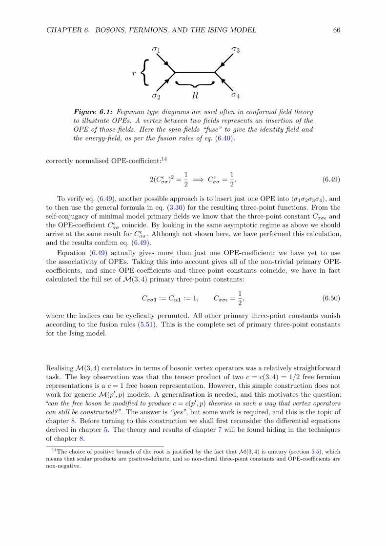
CHAPTER 6. BOSONS, FERMIONS, AND THE ISING MODEL 66
σ1
σ2 σ4
σ3
r
R
Figure 6.1: Feynman type diagrams are used often in conformal field theoryto illustrate OPEs. A vertex between two fields represents an insertion of theOPE of those fields. Here the spin-fields “fuse” to give the identity field andthe energy-field, as per the fusion rules of eq. (6.40).
correctly normalised OPE-coefficient:14
2(Cεσσ)2 =1
2=⇒ Cεσσ =
1
2. (6.49)
To verify eq. (6.49), another possible approach is to insert just one OPE into 〈σ1σ2σ3σ4〉, andto then use the general formula in eq. (3.30) for the resulting three-point functions. From theself-conjugacy of minimal model primary fields we know that the three-point constant Cσσε andthe OPE-coefficient Cεσσ coincide. By looking in the same asymptotic regime as above we shouldarrive at the same result for Cεσσ. Although not shown here, we have performed this calculation,and the results confirm eq. (6.49).
Equation (6.49) actually gives more than just one OPE-coefficient; we have yet to usethe associativity of OPEs. Taking this into account gives all of the non-trivial primary OPE-coefficients, and since OPE-coefficients and three-point constants coincide, we have in factcalculated the full set of M(3, 4) primary three-point constants:
Cσσ1 := Cεε1 := 1, Cσσε =1
2, (6.50)
where the indices can be cyclically permuted. All other primary three-point constants vanishaccording to the fusion rules (5.51). This is the complete set of primary three-point constantsfor the Ising model.
RealisingM(3, 4) correlators in terms of bosonic vertex operators was a relatively straightforwardtask. The key observation was that the tensor product of two c = c(3, 4) = 1/2 free fermionrepresentations is a c = 1 free boson representation. However, this simple construction does notwork for generic M(p′, p) models. A generalisation is needed, and this motivates the question:“can the free boson be modified to produce c = c(p′, p) theories in such a way that vertex operatorscan still be constructed?”. The answer is “yes”, but some work is required, and this is the topic ofchapter 8. Before turning to this construction we shall first reconsider the differential equationsderived in chapter 5. The theory and results of chapter 7 will be found hiding in the techniquesof chapter 8.
14The choice of positive branch of the root is justified by the fact that M(3, 4) is unitary (section 5.5), whichmeans that scalar products are positive-definite, and so non-chiral three-point constants and OPE-coefficients arenon-negative.

CHAPTER 6. BOSONS, FERMIONS, AND THE ISING MODEL 67
6.A Appendix: Fermionic version of Wick’s theorem
Differentiating the defining OPE in 6.1 we have
∂ψ(z)ψ(w) =−1
(z − w)2, ψ(z)∂ψ(w) =
1
(z − w)2, ∂ψ(z)∂ψ(w) =
−2
(z − w)31. (6.51)
Wick’s theorem is modified for free fermions — the prescription in section 4.5 still holds, exceptthat when two fields are being contracted we take them to have first been commuted intoadjacent positions, which results in the gain of a minus sign each time two mutually fermionicfields are commuted with one another. Refer to [6, App. A] for more details. The free fermionenergy-momentum tensor OPE is
LF (z)LF (w) =1
4
(:∂ψ(z)ψ(z):
)(:∂ψ(w)ψ(w):
)= :(regular term): +
1
4
:∂ψ(z)ψ(z)∂ψ(w)ψ(w):− :∂ψ(z)ψ(z)∂ψ(w)ψ(w):
− :∂ψ(z)ψ(z)∂ψ(w)ψ(w): + :∂ψ(z)ψ(z)∂ψ(w)ψ(w):
− :∂ψ(z)ψ(z)∂ψ(w)ψ(w): + :∂ψ(z)ψ(z)∂ψ(w)ψ(w):
. (6.52)
Inserting the OPEs and Laurent expanding the normally ordered terms containing differentarguments, we arrive at the result in eq. (6.2).

Chapter 7
Differential Equations andMonodromy
Minimal model chiral correlation functions satisfy singular vector differential equations, as derivedin chapter 5. Particular solutions to these differential equations are the conformal blocks discussedin section 3.4.1 — the building blocks for physical correlators. Without boundary conditionsindicating how conformal blocks should be combined, one might wonder how physical correlatorscan be constructed. Imposing consistency conditions is key — a physical correlator must besingle-valued, leading to a constraint called monodromy invariance. This constraint specifies howconformal blocks from the holomorphic and anti-holomorphic sectors should be combined, whichallows for the construction of physical correlators even without a set of boundary conditions.
7.1 Four-point functions
In chapter 5 we derived the level 2 singular vector differential equation (5.26). We considered thecase of a primary three-point function, from which we derived fusion rules. Now let us considerthe equation for a primary four-point function:∂2
1 + η2
4∑j=2
[hj
(zj − z1)2− 1
zj − z1∂j
] 〈0|φ1(z1)φ2(z2)φ3(z3)φ4(z4) |0〉 = 0, (7.1)
where η2 is defined in eq. (5.14). Equation (7.1) is satisfied if φ1 has Kac weight h2,1 or h1,2. TheWard identities from section 3.5 determine four-point functions up to an arbitrary differentiablefunction of a single cross-ratio, say
x =z12z34
z14z32. (7.2)
This fact allows one to transform the four-variable partial differential equation in eq. (7.1) into aone-variable ordinary differential equation. See [53, Ch. 8.3] for expressions of N -point functionsinvolving N − 3 cross-ratios. Instead of referring to these general expressions, we will appeal tothe definition of primary fields from eq. (3.1).
The Mobius transformation ω that produces the cross-ratio x is
ω : z 7→ ω(z) =(z − z2)(z3 − z4)
(z − z4)(z3 − z2), (7.3)
which performs the mapping (z1, z2, z3, z4) 7→ (x, 0, 1,∞). Since ω is a conformal transformationthe primary fields transform as
φi(zi) =
(dω
dz
)hi|z=zi
φi(ω(zi)). (7.4)
68

CHAPTER 7. DIFFERENTIAL EQUATIONS AND MONODROMY 69
Writing ωi := ω(zi) we have the corresponding scaling of the correlator
〈0|φ1(z1)φ2(z2)φ3(z3)φ4(z4) |0〉 =4∏i=1
(dω
dz
)hi|z=zi
〈0|φ1(ω1)φ2(ω2)φ3(ω3)φ4(ω4) |0〉 . (7.5)
Denote is as〈0|φ1(z1)φ2(z2)φ3(z3)φ4(z4) |0〉 := FH(x), (7.6)
where H(x) is defined by1
H(x) = 〈φ4|φ3(1)φ1(x) |φ2〉 , (7.7)
and the factor F is
F = z−2h114 z−h1−h2−h3+h4
32 z−h2−h4+h3+h124 z−h3−h4+h2+h1
34 . (7.8)
There is a minor comment to make about deriving this factor. Note that the derivative withrespect to z4 cannot be computed directly from eq. (7.4), because (dω/dz) diverges at z = z4.The subtlety arises from the definition of 〈φ4|, which we defined in eq. (3.14) to be 〈φ4| :=limR→∞R
2h4 〈0|φ4(R). Taking this into account gives a well defined factor. The other derivativescan be computed directly from eq. (7.4).
The function on the right-hand side of eq. (7.6) satisfies the same singular vector equation(7.1) as the four-point function. Note that H(x) depends on only one free parameter x, withthe dependence on each individual zi factored out. This enables us to transform the partialdifferential equation in eq. (7.1) into an ordinary differential equation for H(x), which we canthen solve. This transformation takes a bit of work — see App. 7.A. The result is
d2
dx2− η2
(1
x+
1
x− 1
)d
dx− η2
[h1 + h2 + h3 − h4
x(x− 1)− h3
(x− 1)2− h2
x2
]H(x) = 0. (7.9)
Equation (7.9) appears without a detailed derivation in [9].
7.2 The hypergeometric class
Let us classify eq. (7.9) before attempting to solve it. Refer to [121, Ch. 1,2] for a review ofthe following theory. Equation (7.9) is a linear homogeneous second-order ordinary differentialequation, written in the following standard form:
y′′(x) + P (x)y′(x) +Q(x)y(x) = 0, (7.10)
where x ∈ C and the coefficients P (x) and Q(x) are ratios of polynomials in x. For eq. (7.10) apoint x0 is called ordinary if P (x) and Q(x) are analytic there, otherwise x0 is called a singularpoint. A singular point x0 is called regular if Q(x) has at most a second-order pole at x0 andP (x) at most a first-order pole, or equivalently if (x− x0)2Q(x) and (x− x0)P (x) remain finiteas x→ x0. If this is not the case then the singular point is irregular.
From these definitions we find that both x = 0 and x = 1 are regular singular points ofeq. (7.9). To classify the point at infinity we make the change of variables ξ = 1/x and repeatthe checks for ξ → 0. The point at infinity is also a regular singular point. So eq. (7.9) is a linearhomogeneous second-order ordinary differential equation with three distinct regular singularpoints.
Having only singular points that are regular on S2 := C ∪ ∞ (and a few other minorconditions [121, Sec. 1.1]) puts eq. (7.9) into a class of equations called the Fuchsian class. Inparticular, Fuchsian equations with three singular points constitute the hypergeometric class
1The fields have been rearranged as a reminder of the implicit radial ordering.

CHAPTER 7. DIFFERENTIAL EQUATIONS AND MONODROMY 70
— every equation in this class can be transformed into the famous hypergeometric differentialequation. Make the substitution [67, Ch. 10]
H(x) = xµ(1− x)νG(x) (7.11)
into eq. (7.9), where µ and ν satisfy the indicial equations:2
µ2 − (η2 + 1)µ+ η2h2 = 0, ν2 − (η2 + 1)ν + η2h3 = 0. (7.12)
Substituting eq. (7.11) into eq. (7.9) we get the following differential equation for G(x):
x(1− x)G′′(x) + [c− (a+ b+ 1)x]G′(x)− abG(x) = 0, (7.13)
where a, b, and c satisfy a+ b+ 1 = 2(µ+ ν − η2)
ab = 2µν − (µ+ ν + h1 + h2 + h3 − h4)η2
c = 2ν − η2.
(7.14)
7.2.1 Hypergeometric functions
For brevity, when performing calculations in the remainder of this chapter we shall not present adetailed discussion of convergence issues. App. 7.C contains sufficient convergence informationto verify the calculations in this chapter.
Equation (7.13) is the hypergeometric differential equation.3 Solutions to this equation areknown in terms of the hypergeometric function 2F1(a, b; c;x).4 The hypergeometric functionadmits integral representations. For example, we have the following integral expressions [30,eq. 3,3’]:
2F1(a, b; c;x) =Γ(c)
Γ(b)Γ(c− b)
∫ 1
0tb−1(1− t)c−b−1(1− xt)−adt, (7.15)
=Γ(c)
Γ(b)Γ(c− b)
∫ ∞1
ta−c(t− 1)c−b−1(t− x)−adt. (7.16)
The integral in eq. (7.16) is obtained by making the change of integration variable t 7→ 1/t ineq. (7.15). Both eqs. (7.15) and (7.16) will appear in chapter 8. The hypergeometric function isnormalised so that 2F1(a, b; c; 0) = 1 — the ratio of gamma functions multiplying the integrals isthe reciprocal of Euler’s beta function
β(x, y) =
∫ 1
0tx−1(1− t)y−1dt =
Γ(x)Γ(y)
Γ(x+ y). (7.17)
Equations (7.15) to (7.17) will be important in chapter 8.
A solution to the differential equation in eq. (7.10) is said to be local to a regular singularpoint x0 if it is analytic at x0. The solution in eq. (7.15) to the hypergeometric equation islocal to the singular point at x = 0 (under some convergence conditions given in App. 7.C).
2The exponents µ and ν are called characteristic exponents for the singular points at x = 0 and x = 1respectively.
3The hypergeometric differential equation is the unique second-order linear ordinary differential equation withprecisely three singular points 0, 1, and∞, all of which are regular, with characteristic exponents (0, 1−c), (0, c−a−b)and (a, b) respectively [30, Sec. 1].
4The original solution to the hypergeometric equation dates back to Euler in 1778. The hypergeometric functionhas found outstandingly diverse applications since then — the book [132] on hypergeometric functions deservesspecial mention on this point.

CHAPTER 7. DIFFERENTIAL EQUATIONS AND MONODROMY 71
2F1(a, b; c;x) is analytic within the unit disc centred at x = 0 — whether the disc is open orclosed depends on a, b, and c (App. 7.C).
For a second-order ordinary differential equation we should expect another linearly independentsolution, with the general solution given by a linear combination of the two. Another linearlyindependent solution is [121, Ch. 2]
x1−c2F1(a+ 1− c, b+ 1− c; 2− c;x). (7.18)
The function in eq. (7.18) is also local to x = 0 provided that c < 1 and the hypergeometricfunction converges as per the conditions in App. 7.C.
So, we have a differential equation for a chiral four-point function with φ1(z1) = φ1,2(z1) orφ2,1(z1), and we have found particular solutions. However, we have no boundary conditions totell us how these should be combined to give the physical correlator. The answer to this problemis a consistency condition called monodromy invariance.
7.3 Monodromy and the two-point connection problem
7.3.1 Monodromy
A solution to an ordinary differential equation is often obtained locally about a singular point,for example by series solutions or integrals. If a solution is analytic on its domain then one cantry to analytically continue the solution into a larger domain. If analytic continuation is possible,one can then try to continue the solution back to the original domain. The resulting continuation,if possible, will still solve the ordinary differential equation, but it might be a different solutionto what we started with — the value taken by the original solution might differ from the valuetaken by continued solution even where the arguments coincide. How can one be sure that twoanalytic continuations result in the same solution?
A result from complex analysis called the monodromy theorem [85, Thm. 2.3] says thatfor an analytic function, if two paths of analytic continuation with the same endpoints can becontinuously deformed into one another (that is, without passing over a singular point) thenthe endpoint values of the continuations will agree. The monodromy theorem does not apply topaths that are not continuously deformable to one another, such as those depicted in fig. 7.1.
zj
Figure 7.1: If zj is a singular point, then the two paths illustrated are notcontinuously deformable into one another. If an analytic function is continuedalong these paths, then the values at the endpoints might not agree.
Continuing a solution to a differential equation about a loop is called a monodromytransformation, as depicted in fig. 7.2. If every monodromy transformation acts as the identityoperation on a solution to an equation then that solution is said to be monodromy invariant.In particular a non-zero solution is single-valued if and only if it is monodromy invariant. Physicalcorrelators must be monodromy invariant.
Particular solutions to a differential equation might not be monodromy invariant, but itmay be possible to construct a monodromy invariant solution by taking certain combinations of

CHAPTER 7. DIFFERENTIAL EQUATIONS AND MONODROMY 72
zj
zi
Figure 7.2: Both loops depict monodromy transformations. The upper loop iscontinuously contractible to a point, so the monodromy theorem guarantees thatthe monodromy transformation for this loop acts as the identity on an analyticfunction. If zj is a singular point then the same cannot be said for the lowerloop.
particular solutions. To do so we need to determine how each particular solution to the differentialequation transforms under monodromy transformations.5 Understanding this procedure is thegoal of section 7.3.2.
7.3.2 The two-point connection problem
Local to each singular point (all of which are regular) of eq. (7.13) one can construct standardfundamental sets of solutions.6 Two standard solutions local to x = 0 are given by
2F1(a, b; c;x), x1−c2F1(a+ 1− c, b+ 1− c; 2− c;x). (7.19)
These are linearly independent, and analytic within the unit disc about x = 0. There is also apair of fundamental solutions local to x = 1 given by [121, Ch. 2]
2F1(a, b; a+ b+ 1− c; 1− x), (1− x)c−a−b2F1(c− a, c− b; 1 + c− a− b; 1− x). (7.20)
These are linearly independent, and analytic within the unit disc about x = 1. Another pair ofsolutions local to x =∞ can be found by making the change of variables ξ = 1/x and searchingfor solutions local to ξ = 0. For reasons that will be explained later we do not need to considersolutions local to x =∞.
For a second-order linear differential equation, how do we end up with 6 solutions? The answerof course is that they are not all linearly independent. Any pair of solutions can be analyticallycontinued into any other by a linear transformation7 — we say that the transformation connectsone solution to another. Finding the transformation that connects pairs of solutions is called aconnection problem.
For example, we write the solutions local to x = 0 as a column vector:
F0(x) :=
[f
(0)1 (x)
f(0)2 (x)
]:=
[2F1(a, b; c;x)
x1−c2F1(a+ 1− c, b+ 1− c; 2− c;x)
], (7.21)
and local to x = 1 as
F1(x) :=
[f
(1)1 (x)
f(1)2 (x)
]:=
[2F1(a, b; a+ b+ 1− c; 1− x)
(1− x)c−a−b2F1(c− a, c− b; 1 + c− a− b; 1− x)
]. (7.22)
5This has a nice interpretation as finding a representation for the monodromy group [30].6Sometimes these are called Frobenius solutions. They can be found using the well known Frobenius method,
which consists of looking for series solutions and deriving recursion relations for the series coefficients.7For the hypergeometric differential equation there are 24 such pairings, known as Kummer’s relations [120].
CHAPTER 7. DIFFERENTIAL EQUATIONS AND MONODROMY 73
We do not need to consider the solutions F∞(x) local to ∞. The solutions F0(x) and F1(x) areconnected by a 2× 2 matrix T called a connection matrix:
F0(x) = TF1(x). (7.23)
The connection matrix T is a constant matrix whose coefficients depend on the parameters a, b,and c. The coefficients can be determined by considering the values taken by the fundamentalsolutions in eqs. (7.21) and (7.22) at specific values of x, which we can compute using the integralrepresentation in eq. (7.15).
Firstly, setting x = 1, the integral in eq. (7.15) becomes an integral representation for Euler’sbeta function from eq. (7.17), and we obtain
2F1(a, b; c; 1) =Γ(c)
Γ(b)Γ(c− b)Γ(c− a− b)Γ(b)
Γ(c− a)=
Γ(c)Γ(c− a− b)Γ(c− b)Γ(c− a)
. (7.24)
The real integral converges if and only if b and c − a − b are positive, but the final ratio ineq. (7.24) is the unique analytic continuation defined wherever the ratio of gamma functions isfinite [121, Ch. 2.4].
Using the result in eq. (7.24), and the fact that the hypergeometric function is normalised sothat 2F1(a, b; c; 0) = 1, we can compute F0(0),F0(1),F1(0), and F1(1) explicitly. For example,
assuming we have 0 < c < 1 it follows that f(0)2 (0) = 0 due to the factor of x1−c in eq. (7.21)
and finiteness of 2F1(a, b; c; 0) = 1. Similarly, assuming we have 0 < c− a− b < 1 it follows that
f(1)2 (1) = 0. Substituting these values of x into eq. (7.23) we obtain the following linear system
of equations [10
]= T
[f
(1)1 (0)
f(1)2 (0)
],
[f
(0)1 (1)
f(0)2 (1)
]= T
[10
]. (7.25)
The remaining values of f(j)i (0) and f
(j)i (1) can all be determined from eq. (7.24) and the
normalisation 2F1(a, b; c; 0) = 1. The connection coefficients can then be found by inverting thelinear system in eq. (7.25). Solving the system we find that
T11 =Γ(c)Γ(c− a− b)Γ(c− a)Γ(c− b)
, T12 =Γ(c)Γ(a+ b− c)
Γ(a)Γ(b),
T21 =Γ(2− c)Γ(c− a− b)
Γ(1− a)Γ(1− b), T22 =
Γ(2− c)Γ(a+ b− c)Γ(a+ 1− c)Γ(b+ 1− c)
. (7.26)
A derivation of eq. (7.26) is given in App. 7.B.
We are now in a position to compute monodromy transformations for the solutions to theequation. Our differential equation has S2\0, 1,∞ as its domain, and the solution space isclosed under continuations in this domain. A monodromy transformation about any point willtherefore act as a 2× 2 transformation matrix on the vectors of solutions F0(x) and F1(x).
Monodromy about 0
For the solutions F0(x), which are analytic within the unit disc centred at x = 0, we can explicitlycompute the monodromy transformation about x = 0. Denote by M0 the monodromy operatorthat acts on x, taking it once about the origin in an anticlockwise loop that encloses no singularpoints except for the origin. The associated monodromy transformation about the origin is
F0(x) 7→ F0(M0 · x) = (M0)F0(x), (7.27)
where (M0) is a 2× 2 matrix called the monodromy matrix of the operator M0.

CHAPTER 7. DIFFERENTIAL EQUATIONS AND MONODROMY 74
We can parametrise the action of M0 explicitly. We choose a circular loop γ0 : [0, 1]→ C\0, 1given by
γ0(κ) := xe2πiκ, (7.28)
which starts and ends at x, and encircles the origin once, avoiding all singular points. Theonly singular point it encloses is at the origin, because the radial ordering we have assumed is0 < |x| < 1.
We can find the matrix (M0) by substituting γ0(κ) for x in eq. (7.21) and taking κ continuouslyfrom 0 to 1. The hypergeometric function 2F1(a, b; c;x) is unchanged by M0, since 2F1(a, b; c;x)is analytic within the unit disc centred at the origin. However, we do gain a phase from thefactor x1−c, and we derive the matrix
(M0) =
(1 00 e−2πic
). (7.29)
Note that (M0) is diagonal and the solutions in F0(x) are unchanged up to phase — this isimportant, but we will have to wait until chapter 8 to appreciate why.
Monodromy about 1
The monodromy transformation M1 which takes x about 1 corresponds to the transformationF0(x) 7→ F0(M1 · x) = (M1)F0(x). To determine (M1) one might try to explicitly parametrisethe transformation, as we did before using γ0(κ), but then one quickly runs into a problem —the integrals in eqs. (7.15) and (7.16) that define F0(x) diverge if x is taken out of the unit disccentred at the origin. However, the transformation can be easily computed for F1(x), which isconvergent within the unit disc about x = 1. Denote the corresponding monodromy matrix by(M ′1) so that we have F1(M1 · x) = (M ′1)F1(x). If we make the substitution x′ = 1− x in F1(x),and compare the resulting expressions to the monodromy transformation about 0 for F0(x), thenfrom eq. (7.29) we read off
F1(x) 7→ F1(M1 · x) = (M ′1)F1(x) =
(1 0
0 e2πi(c−a−b)
)F1(x). (7.30)
Now we come to the point of all of this. The matrix (M1) can be determined by firstconnecting F0(x) to F1(x), then performing the monodromy transformation M1 using the knownmonodromy matrix (M ′1), and then connecting the result back to F0(x):
(M1)F0(x) = F0(M1 · x) = TF1(M1 · x) = T (M ′1)F1(x) = T (M ′1)T−1F0(x). (7.31)
The monodromy matrix (M1) is therefore given by
(M1) = T (M ′1)T−1. (7.32)
With a few gamma function manipulations similar to those in App. 7.B and section 8.8 wefind that the determinant of the connection matrix is
detT = T11T22 − T12T21 =1− c
a+ b− c. (7.33)
Our previous assumptions that 0 < c < 1 and 0 < c− a− b < 1 therefore guarantee invertibilityof T . The inverse connection matrix takes the simple form:
T−1 =a+ b− c
1− c
(T22 −T12
−T21 T11
). (7.34)

CHAPTER 7. DIFFERENTIAL EQUATIONS AND MONODROMY 75
∞
1
0
x
∞
1
0
x
∞
1
0
x
A B C
Figure 7.3: Monodromy transformations on the Riemann Sphere.A: Monodromy transformations M0 and M1. B: Invariance with respect toM0 and M1 implies invariance with respect to the transformation enclosingboth points 0 and 1. C: The transformation in B is equal to M−1
∞ , the inversetransformation about ∞. Hence invariance with respect to both M0 and M1
implies that M−1∞ acts as the identity, and therefore so does M∞.
From eqs. (7.32) and (7.34) we can calculate the monodromy matrix (M1):
(M1) =a+ b− c
1− c
(T11 T12
T21 T22
)(1 0
0 e2πi(c−a−b)
)(T22 −T12
−T21 T11
). (7.35)
From these expressions, and by considering the anti-holomorphic sector, we can constructthe physical correlation functions we have been seeking, assuming that such functions exist.
7.3.3 The anti-holomorphic sector
In the anti-holomorphic sector we derive expressions that are the complex conjugates of thosein the holomorphic sector. The physical correlation function can be obtained by combiningchiral conformal blocks from the holomorphic and anti-holomorphic sectors in a monodromyinvariant way. We will demonstrate this procedure in detail in section 8.5.1 (although from adifferent starting point) and so for now we shall just briefly outline the corresponding methodusing connection and monodromy matrices.
The transformed chiral correlation function G(x) from eq. (7.11) and the correspondinganti-holomorphic function G(x) are to be combined into a function G(x, x), which is expandedin terms of particular solutions to eq. (7.13) as
G(x, x) =2∑
i,j=1
Xijf(0)i (x)f
(0)j (x), (7.36)
where (Xij) is a 2× 2 constant matrix whose coefficients can be fixed by imposing monodromyinvariance. As will be discussed in section 8.5.1 the corresponding physical correlation function issingle-valued if and only if the matrix coefficients Xij are selected so that G(x, x) is monodromyinvariant.
Note from fig. 7.3 that if G(x, x) is invariant with respect to M0 and M1 then it is automaticallyinvariant with respect to M∞. This is the reason that we have not considered the solutionsF∞(x), nor have we calculated the monodromy matrix (M∞).
The monodromy transformation M0 can be calculated explicitly using the monodromy matrix(M0) from eq. (7.29). When acting with M0 on the conjugate variable x, the orientation of the

CHAPTER 7. DIFFERENTIAL EQUATIONS AND MONODROMY 76
loop is reversed, and the corresponding monodromy matrix (M0) is the complex conjugate of(M0). We therefore find that G(x, x) transforms as
G(x, x) 7→ G(M0 · x,M0 · x) =
2∑i,j,k,l=1
Xij(M0)ik(M0)jlf(0)k (x)f
(0)l (x). (7.37)
Similarly, the monodromy transformation M1 can be calculated using the monodromy matrix(M1) from eq. (7.35), and we find that
G(x, x) 7→ G(M1 · x,M1 · x) =2∑
i,j,k,l=1
Xij(M1)ik(M1)jlf(0)k (x)f
(0)l (x). (7.38)
If we demand that M0 and M1 act as the identity on the function in eq. (7.36) so that thetransformed expansions in eqs. (7.37) and (7.38) are equal to the untransformed expansion ineq. (7.36), then the matrix coefficients Xij satisfy a linear system of equations involving thematrix coefficients of the monodromy matrices (M0) and (M1). Solving this system for (Xij)allows one to construct a single-valued physical correlator.8
Instead of continuing with this calculation here we shall turn now to the Coulomb gasformalism. The problem of combining conformal blocks to construct a physical correlationfunction will be revisited and completed using the Coulomb gas formalism in section 8.5. Thethe work we have already done in this chapter will not go unrewarded, for in section 8.8 theconnection transformations for hypergeometric functions will be revealed to be lurking withinthe Coulomb gas formalism.
7.A Appendix: From PDE to ODE
This appendix explains the transformation of the partial differential equation eq. (7.1) into theordinary differential equation eq. (7.9). Write the factor F from eq. (7.6) as
F = zA1414 zA32
32 zA2424 zA34
34 , (7.39)
with the exponents given by
A14 = −2h1, A32 = −h1 − h2 − h3 + h4,
A24 = −h2 − h4 + h1 + h3, A34 = −h3 − h4 + h1 + h2. (7.40)
The transformation of eq. (7.1) begins by application of the chain rule:
∂
∂ziFH(x) =
∂F
∂ziH(x) + F
∂x
∂zi
dH
dx. (7.41)
The double derivative with respect to z1 is
∂2
∂z21
FH(x) =∂2F
∂z21
H(x) + 2∂F
∂z1
∂x
∂z1
dH
dx+ F
∂2x
∂z21
dH
dx+ F
(∂x
∂z1
)2 d2H
dx2. (7.42)
8Actually the overall normalisation is not fixed by solving the linear system, but in section 8.5 we willdemonstrate how the normalisation can be fixed.

CHAPTER 7. DIFFERENTIAL EQUATIONS AND MONODROMY 77
Although perhaps tedious, the derivatives are all easy to calculate. Substituting them into thesingular vector partial differential equation (7.1) we find that
0 =
∂2
∂z21
+ η2
4∑j=2
[hjz2
1j
+1
z1j
∂
∂zj
]FH(x)
= F
A14(A14 − 1)
z214
+
(2A14
z14
[z34
z14z32− z12z34
z214z32
]− 2
z34
z214z32
+ 2z12z34
z314z32
)d
dx
+
(z34
z14z32− z12z34
z214z32
)2 d2
dx2+ η2
(h2
z212
+h3
z213
+h4
z214
+1
z12
[−A32
z32+A24
z24
(− z34
z14z32+z12z34
z14z232
)d
dx
]+
1
z13
[A32
z32+A34
z34+
(z12
z14z32− z12z34
z14z232
)d
dx
]+
1
z14
[−A14
z14− A24
z24− A34
z34+
(− z12
z14z32+z12z34
z214z32
)d
dx
])H(x). (7.43)
The factor F has now been factored out, and so what remains must vanish. Performing theMobius transformation in eq. (7.3) we are left with
0 =
d2
dx2+ η2
[h2
x2+
h3
(x− 1)2+
1
x
[−A32 + (x− 1)
d
dx
]+
1
x− 1
[A32 − x
d
dx
]]H(x) (7.44)
Replacing A32 by its value −h1 − h2 − h3 + h4, we arrive at the ordinary differential equationgiven in eq. (7.9).
7.B Appendix: Connection coefficients
In this appendix we solve the linear system in eq. (7.25) and derive the connection coefficients ineq. (7.26). The linear system in eq. (7.25) for the connection coefficients can be written as
1 = T11f(1)1 (0) + T12f
(1)2 (0), 0 = T21f
(1)1 (0) + T22f
(1)2 (0), (7.45)
f(0)1 (1) = T11, f
(0)2 (1) = T21. (7.46)
The coefficients T11 and T21 are easily computed using eq. (7.24). We shall demonstrate thecalculation of T22. The coefficient T12 is calculated in a similar manner.
Firstly, using eq. (7.24) we find that
T21 = 2F1(a+ 1− c, b+ 1− c; 2− c; 1) =Γ(2− c)Γ(c− a− b)
Γ(1− b)Γ(1− a), (7.47)
f(1)1 (0) = 2F1(a, b; a+ b+ 1− c; 1) =
Γ(a+ b+ 1− c)Γ(1− c)Γ(a+ 1− c)Γ(b+ 1− c)
, (7.48)
f(1)2 (0) = 2F1(c− a, c− b; 1 + c− a− b; 1) =
Γ(1 + c− a− b)Γ(1− c)Γ(1− a)Γ(1− b)
. (7.49)
Solving eq. (7.45) for T22 gives
T22 = −T21f
(1)1 (0)
f(1)2 (0)
=−Γ(2− c)
Γ(a+ 1− c)Γ(b+ 1− c)
[Γ(c− a− b)Γ(a+ b+ 1− c)
Γ(1 + c− a− b)
]. (7.50)

CHAPTER 7. DIFFERENTIAL EQUATIONS AND MONODROMY 78
The second factor in square brackets can be simplified using Euler’s reflection identity
Γ(1− x)Γ(x) =π
sin(πx), (7.51)
which makes the calculation of detT easier, and will be convenient for proving some identities insection 8.8. The factor becomes[
π
sinπ(c− a− b)sinπ(−c+ a+ b)
πΓ(a+ b− c)
]= −Γ(a+ b− c). (7.52)
Substituting this back into eq. (7.50), we arrive at the result in eq. (7.26).
7.C Appendix: Convergence information
The following convergence information is from [121]. The necessary convergence conditions aresatisfied in the example that we encounter in chapter 8. In particular we will not need to worryabout the taking the real and imaginary parts of a, b, and c, because they will be real. However,for the sake of completeness we still state the convergence information in its general form below.
• The integrals in eqs. (7.15) and (7.16) converge in the Cauchy principal value sense ifRe (c) > Re (b) > 0 and |x| < 1, or |x| = 1 and Re (c− b− a) > 0 and Re (b) > 0. Wefrequently used the phrase “within the unit disc” for domains of convergence — that discis open in the former case and closed in the latter.
• The integral in eq. (7.17) for Euler’s beta function converges as a principal value integralfor Re (x),Re (y) > 0.
• For the local sets of solutions in eqs. (7.21) and (7.22) we have assumed that c /∈ Z.
Chapter 8
The Coulomb Gas Formalism
Vertex operators are spectacularly useful in conformal field theory. For one thing their correlationfunctions are all known. Moreover they have explicit mode expansions in terms of the Heisenbergalgebra, making them easy to manipulate. Translating Ising model correlation functions intoproblems involving vertex operators allowed us to compute them in a few pages of work.
Herein lies the power of the Coulomb gas formalism. It allows one to realise minimal modelcorrelation functions in terms of vertex operators and, on top of that, provides a way to systemat-ically stitch together monodromy-invariant solutions to singular vector differential equations usingtechniques of contour integral manipulation. Lurking beneath the contour manipulations arelinks to many ostensibly unrelated areas, one such area being the hypergeometric-type connectionproblem from chapter 7.
In this chapter we combine the knowledge from all previous chapters — the minimal modelsof chapter 5 are realised using screening operators, which are constructed from the bosonic vertexoperators of chapter 4; the bosonisation calculations of chapter 6 are verified; we identify linksto the singular vector differential equations from chapter 7; we relate contour manipulations tothe monodromy problem and the two-point connection problem of section 7.3; and finally wedemonstrate the power of the Coulomb gas formalism by providing complete sets of primaryOPE-coefficients for three different minimal model theories, both main series and not.
Why is it called the “Coulomb gas” formalism?
In section 4.7, the OPE of the free boson anti-derivative φ(z) in eq. (4.52) was found to beφ(z)φ(w) ∼ log(z − w), and in two dimensions the Coulomb electric potential between twocharges separated by a displacement |z−w| is proportional to log |z−w|. Vertex operators, whichplay a crucial role in the Coulomb gas formalism, are given by normally ordered exponentials ofthe field φ(z). Moreover, many integral expressions that arise in the formalism closely resemblethose of log-gases in statistical mechanics [51].
8.1 Modifying the free boson
Let us begin by playing some games with the representation theory of the free boson. Considerthe field obtained if we modify the free boson energy-momentum tensor by appending to it theterm ∂2ϕ(z):
LA(z) =1
2:∂ϕ(z)∂ϕ(z): +A∂2ϕ(z), (8.1)
where A ∈ C is for the moment unspecified. This modification is actually not so out-of-the-blue— the free boson energy-momentum tensor is modified in this way if the Lagrange density ofeq. (4.3) is coupled to the scalar curvature of a curved manifold — see [53, Ch. 9.1.3]. This
79

CHAPTER 8. THE COULOMB GAS FORMALISM 80
Table 8.1: Coulomb gas modifications
Free boson Coulomb gas
c 1 1− 12A2
Ln1
2
∑r∈Z :an−rar:
12
∑r∈Z :an−rar:−A(n+ 1)an
L(z)∂ϕ(w) ∼ ∂ϕ(w)
(z − w)2+∂2ϕ(w)
z − w∼ −2A
(z − w)31 +
∂ϕ(w)
(z − w)2+∂2ϕ(w)
z − w
L(z)Vp(w) ∼(1
2p2)Vp(w)
(z − w)2+∂Vp(w)
z − w∼
(12p
2 −Ap)Vp(w)
(z − w)2+∂Vp(w)
z − wL0 |p〉 1
2p2 |p〉 (1
2p2 −Ap) |p〉
modification can be interpreted as the influence of a “background charge” located at infinity, andthe Coulomb gas theory can be interpreted as a perturbation of the free boson theory caused bythis charge.
To check if this modification still defines a conformal field theory we need to check if LA(z)satisfies the defining OPE for a conformal energy-momentum tensor. An application of Wick’stheorem, shown in App. 8.A, gives
LA(z)LA(w) ∼ (1− 12A2)/2
(z − w)41 +
2LA(w)
(z − w)2+∂LA(w)
z − w, (8.2)
which is still the defining OPE of a Virasoro symmetry field, but with modified central charge.Using the range of techniques we have developed so far we can determine how the Coulombgas theory is modified from the standard free boson theory. These modifications are shown intable 8.1.
In the Coulomb gas formalism the central charge is c = 1− 12A2 and the conformal weightof the Heisenberg vacuum |p〉 is hp = 1
2p2 − Ap. For A 6= 0 the field ∂ϕ(z) is not a Virasoro
primary field, since it does not satisfy the defining OPE in eq. (3.11) for a Virasoro primary withthe energy-momentum tensor, but vertex operators remain Virasoro primaries, although withmodified conformal weight.
8.2 Screening fields
There exist special fields called screening fields, which are essential in constructing the minimalmodels and their correlation functions.
Consider a generic Virasoro primary field S(w) with conformal weight hS and with modeexpansion of the form
S(w) =∑n
Snw−n−hS , (8.3)
where the values taken by the index n depend on the field S(w) and what it acts on. In thespecial case where hS = 1, the residue S0 of S(w) commutes with the Virasoro algebra, and soconstitutes a Vir-module homomorphism (an intertwiner), assuming that this residue is welldefined. This is equivalent to the residue commuting with the energy-momentum tensor, whichgenerates the Virasoro algebra. To show this we use the contour subtraction method fromsection 3.7.1 and fig. 3.1:1
[S0, LA(z)] =
∮zRLA(z)S(w)whS−1 dw
2πi=
∮z
hSS(w)
(z − w)2+∂S(w)
z − w
whS−1 dw
2πi. (8.4)
1We have used RS(w)LA(z) = RLA(z)S(w), which is proven in [92, App. B].
CHAPTER 8. THE COULOMB GAS FORMALISM 81
If hS = 1 then the integrand is a derivative, and the integral becomes∮z
∂
∂w
S(w)
z − w
dw
2πi. (8.5)
If the contour is closed then there are no boundary terms, and the integral vanishes, giving
[S0, LA(z)] = 0. (8.6)
So S0 is a Vir-module homomorphism.
There are some complications, because S(w) is not a function, but some quantum field, and isnot necessarily single-valued. Closure of the contour depends on which field S(w) is and what itacts on. Detailed considerations can be technical — see [125, Sec. 5]. Suffice it to say that therewill be an appropriate choice of integral so that eq. (8.6) holds in each case that we encounter.
Let us consider which primary fields are available in the theory that have conformal weighth = 1. The field ∂ϕ(z) has conformal weight h = 1, but table 8.1 shows that, for A 6= 1, ∂ϕ(z) isnot a Virasoro primary field in the Coulomb gas theory. However, every vertex operator Vp(z) isa Virasoro primary field. Vp(z) has conformal weight hp = 1
2p2 −Ap, and setting hp = 1 we find
two solutions for p:1
2p2 −Ap = 1 =⇒ p± = A±
√A2 + 2. (8.7)
The corresponding vertex operators are denoted by V±(z) — we call them screening fields.
8.3 Realising the minimal models
When we first introduced the Heisenberg algebra we normalised the generators so that the centralelement k acted as the identity operator. For current purposes it will be convenient to work in arenormalised basis so that k acts as multiplication by 2. Make the change of notation
bn :=√
2 an, b :=√
2 a, A :=√
2 α0. (8.8)
The commutation relations are
[bn, bm] = 2nδn,−m, [bn, k] = 0, [bn, b] = 2δn,0, [b, k] = 0, (8.9)
and the Virasoro modes from table 8.1 take the form
Ln =1
4
∑m∈Z
:bn−mbm:− α0(n+ 1)bn. (8.10)
The corresponding vertex operators have mode expansions
Vα(z) := eαbzαb0∞∏n=1
exp
(αbn
z−n
n
)exp
(−αb−n
zn
n
). (8.11)
The state |α〉 corresponding to Vα(z) is a highest weight state for H that satisfies b0 |α〉 = 2α |α〉.The b0-eigenvalue 2α will be called the charge of |α〉.
With the rescaling, table 8.1 determines the conformal weight of |α〉 to be h(α) = α(α− 2α0),reminiscent of the value in eq. (5.33). The two screening fields with conformal weight h(α) = 1have charges:
h(α) = 1 =⇒ α = α± = α0 ±√α2
0 + 1. (8.12)
We call these screening charges. Table 8.1 determines α0 in terms of the central charge c — itturns out to be precisely that of eq. (5.23) from the Kac determinant. The screening charges α±
CHAPTER 8. THE COULOMB GAS FORMALISM 82
are also determined in terms of c from eq. (8.12), and solving for them reproduces the values ineq. (5.23). Finally, if we define the charges αr,s as per eq. (5.34), then we recover from table 8.1the corresponding conformal weights h(αr,s) = hr,s, which are the Kac weights from eqs. (5.22)and (5.35). Using the renormalised basis of Heisenberg generators, the vertex operators in theCoulomb gas formalism reproduce the values from the Kac determinant. Moreover, if the centralcharge takes a minimal model value c = c(p′, p) as per eq. (5.47), then the translation andreflection symmetries of the Kac table in eq. (5.50) are also realised:
hr,s = hr+p′,s+p ↔ h(αr,s) = h(αr+p′,s+p), (8.13)
hr,s = h−r,−s ↔ h(αr,s) = h(α−r,−s) = h(2α0 − αr,s). (8.14)
For a given c(p′, p) the Coulomb gas vertex operators with charges αr,s corresponding to(r, s) in the Kac table (5.50) reproduce all of the M(p′, p) conformal weights. In fact in [41] it isproven that for a given minimal model M(p′, p) each irreducible representation QV (hr,s, c(p
′, p))is isomorphic to a certain quotient of a submodule of the collection of bosonic Fock spaces in thec = c(p′, p) Coulomb gas theory.
Substituting c(p′, p) into eq. (8.12) we find that the screening charges α± can be expressed interms of the coprime integers p′, p as
α+ =√p/p′, α− = −
√p′/p. (8.15)
Note that the ratio α+/α− = −p/p′ is rational.
The idea behind the Coulomb gas formalism
The vertex operator Vαr,s(z) := Vr,s(z) has the same conformal weight as the minimal modelfield φr,s(z). When bosonising the Ising model in section 6.4 the idea was to compute Isingcorrelation functions by first relating to each M(3, 4) primary field a vertex operator with thesame conformal weight, and then computing vertex operator correlators instead, which are allknown from the general formulae in eqs. (4.67) and (4.82). The Coulomb gas formalism extendsthis prescription to all minimal models.
There is still an issue to address — by reflection symmetry the vertex operator V2α0−αr,s(z) =V−r,−s(z) also has conformal weight hr,s, so there seems to be some freedom in which vertexoperator is chosen to represent φr,s(z). This is something we encountered in chapters 4 and 6,where the vertex operators Vp(z) and V−p(z) had the same conformal weight. To constructmeaningful correlation functions we chose combinations of vertex operators that satisfied theconservation of momentum condition of sections 4.4 and 4.6.1. The same idea applies to theCoulomb gas formalism, with some modification.
8.4 Neutrality
The conservation of momentum condition of section 4.4 has an analogue in the Coulomb gasformalism, here interpreted as conservation of charge. We can derive this condition from theexpression for the Virasoro algebra in terms of the Heisenberg algebra in table 8.1.
8.4.1 Neutrality on the level of states
Virasoro modules are embedded in Fock spaces in the same way as in section 4.3.1. The Fock spaceF(α) = U(Hc) |α〉 with highest weight vector |α〉 has the conformal grading into L0-eigenspaces:F(α) =
⊕∞N=0FN (α), where FN (α) is an L0-eigenspace with eigenvalue h(α) +N . We construct
the scalar product as per chapters 4 and 5 with an adjoint map L†n = L−n. The fact that L0 isself-adjoint ensures that different grades are orthogonal.

CHAPTER 8. THE COULOMB GAS FORMALISM 83
Unlike the case in section 4.4, here we do not have a choice as to what the Heisenberg adjointmap can be — from eq. (8.10) for the Virasoro algebra in terms of H, we find that the onlyHeisenberg adjoint map that gives the correct Virasoro adjoint is:
b†n = 4α0δn,0 − b−n, k† = k. (8.16)
The constant term 4α0δn,0 has non-trivial consequences for the scalar product. For example, forvacuum vectors |α〉 and |β〉 labelled by their charges, we have
(b†0 |α〉 , |β〉) = (|α〉 , b0 |β〉) =⇒ (4α0 − 2α)(|α〉 , |β〉) = 2β(|α〉 , |β〉), (8.17)
so |α〉 and |β〉 are orthogonal if β 6= 2α0 − α. Moreover since b0 belongs to the centre Z(H), itfollows that every vector in F(α) is orthogonal to every vector in F(β) if β 6= 2α0 − α. Thecovector 〈α| ∈ F∨(α) is dual not to |α〉, but to |2α0 − α〉 ∈ F(2α0 − α), and from the reflectionsymmetry of eq. (8.14) it is clear that the vector and its dual do indeed have the same conformalweight.
Every covector in F∨(α) maps to zero every vector that is not in F(2α0 − α). With theconventional normalisation: 〈α|2α0 − α〉 := 1, we have the condition
〈α|β〉 = δβ=2α0−α =⇒ 〈0|β〉 = δβ=2α0 . (8.18)
This is called the neutrality condition. The value 2α0 is the aforementioned “backgroundcharge”. Scalar products vanish if the sum of charges is not equal to the background charge,which is the origin of the name “neutrality condition”.
8.4.2 Neutrality for correlation functions
There is a corresponding neutrality condition on the level of vertex operators. Using the generalformula in eq. (4.67) for vertex operator correlation functions, and the neutrality condition ineq. (8.18), we find that
〈0| Vα1(z1) . . .Vαn(zn) |0〉 = δα1+···+αn=2α0
∏i<j
z2αiαjij , (8.19)
which vanishes if∑n
i=1 αi 6= 2α0. This is the neutrality condition for correlation functions.
8.4.3 Neutrality and conservation of momentum
The neutrality condition is analogous to the conservation of momentum condition for the freeboson in section 4.4. Indeed taking α0 = 0 (equivalently taking c = 1), eq. (8.18) becomesthe conservation of momentum condition. This should be expected, because in this limit theCoulomb gas theory coincides with the free boson theory. This is the reason that we chose a0 tobe anti -self-adjoint rather than the conventional self-adjoint in section 4.4. Had we followed theconventional route and chosen a0 to be self-adjoint then the c = 1 limit would not reproduce thefamiliar free boson theory, which would invalidate the interpretation of the Coulomb gas theoryas a perturbation of the free boson theory.
8.4.4 Neutrality and screening operators
To construct minimal model correlation functions one associates to each minimal model fieldφr,s(z) one of the vertex operators Vr,s(z) or V−r,−s(z), which have the same conformal weighthr,s. For example, to construct a two-point function such as
〈0|φr,s(z)φr,s(w) |0〉 , (8.20)
CHAPTER 8. THE COULOMB GAS FORMALISM 84
one might try two-point functions of the form
〈0| Vr,s(z)Vr,s(w) |0〉 , 〈0| V−r,−s(z)V−r,−s(w) |0〉 . (8.21)
We encounter a problem that we have seen before in section 6.4 — although the vertex operatorshave the correct conformal weights, the correlation functions vanish because the neutralitycondition is not satisfied. To see this explicitly, note from eq. (5.22) that αr,s+αr,s = α2r−1,2s−1 6=2α0 for (r, s) in the Kac table Tp′,p. However, both combinations V±r,±s(z) and V∓r,∓s(w) dosatisfy the neutrality condition since αr,s + α−r,−s = α+ + α− = 2α0. Using eq. (8.19) we have
〈0| Vr,s(z)V−r,−s(w) |0〉 =1
(z − w)2αr,s(2α0−αr,s)=
1
(z − w)2hr,s, (8.22)
which reproduces the correctly normalised general solution to the two-point function in eq. (3.31).The vertex operators Vr,s(z) and V−r,−s(z) are conjugate fields. For valid two-point functions theneutrality condition can always be satisfied by selecting the vertex operators to be conjugates.When more fields are involved this is no longer true.
For instance, consider a chiral M(p′, p) primary correlator of the form 〈0|φr,sφr,sφr,sφr,s |0〉.Since minimal model primaries are self-conjugate it follows that this correlator is necessarilynon-zero — this can be confirmed by inserting an OPE between any two adjacent fields and thenusing the general solution in eq. (3.30) for three-point functions. The available vertex operatorsfor representing each field are Vαr,s and V2α0−αr,s . However, for α0 6= 0 it seems that there is nocombination of these such that the neutrality condition is satisfied. For example, both correlators〈0| Vr,sVr,sVr,sV−r,−s |0〉 and 〈0| Vr,sVr,sV−r,−sV−r,−s |0〉 vanish if α0 6= 0, since neither satisfiesthe neutrality condition.
The resolution to this issue comes in the form of the screening fields from section 8.2. Thetwo screening fields V+(z) and V−(z) are vertex operators with conformal weight h = 1. Theresidues Q+ and Q− of these fields are integral operators called screening operators. Theyare Vir-module homomorphisms since they commute with the energy-momentum tensor — theyshift charges, but not conformal weights. Q+ has charge α+, and Q− has charge α−, and neitheralters the conformal weight of any vector it acts upon. The idea is to insert screening operatorsinto correlation functions so that neutrality is satisfied, but OPE-coefficients are not altered.
There are various approaches to using screening operators, and we will use the prescriptionfrom the original works [34,35]. As was the case in section 6.4, the minimal model OPE-coefficientscan be determined from four-point functions by inserting OPEs and considering asymptotics. Toconstruct a minimal model primary four-point function of the form
〈0|φr1,s1(z1)φr2,s2(z2)φr3,s3(z3)φr4,s4(z4) |0〉 (8.23)
we replace the fields by their associated vertex operators and insert as many screening operatorsas required to satisfy the neutrality condition. Since the conjugate operator V−r,−s(z) =V2α0−αr,s(z) has charge 2α0 − αr,s, including just one conjugate field (conventionally the onelabelled V−r4,−s4(z4)) takes care of the background charge 2α0, as required by the neutralitycondition, and we arrive at a correlation function of the form
〈0|Qm−− Qm++ Vr1,s1(z1)Vr2,s2(z2)Vr3,s3(z3)V−r4,−s4(z4) |0〉 . (8.24)
The integers m+ and m− are chosen in order to satisfy the neutrality condition:
αr1,s1 + αr2,s2 + αr3,s3 +m+α+ +m−α− = αr4,s4 . (8.25)
Since α+ and α− are not independent there might be more than one charge-neutral choicefor m+ and m−. For example, observe from eq. (8.15) that
m+α+ +m−α− =α+
p(m+p−m−p′), (8.26)
CHAPTER 8. THE COULOMB GAS FORMALISM 85
and that this expression is invariant under the shift (m+,m−) 7→ (m+ + p′,m− + p).2 One wayto determine a valid choice is by using the relations
αr,s + αr′,s′ = αr+r′−1,s+s′−1, αr,s +mα+ = αr−2m,s, αr,s +mα− = αr,s−2m, (8.27)
which are straightforward to check using eq. (5.34). It follows that eq. (8.25) is satisfied if m+
and m− are chosen as
m+ =r1 + r2 + r3 − r4 − 2
2, m− =
s1 + s2 + s3 − s4 − 2
2. (8.28)
If this expression does not return integers for m+ and m− then the neutrality condition cannotbe satisfied for that combination of vertex operators Vαi , and the correlation function vanishes.If a negative integer is returned then one can use (m+,m−) 7→ (m+ + p′,m− + p).
Screening operators are integral operators of the form
Q± =
∮V±(u)du, (8.29)
where the meaning of the integral will be specified in section 8.5. The symbols Qm±± are
instructions to insert m± screening fields V±, and then perform m± integrals over the integrand
〈0| V−(u1) . . .V−(um−)V+(v1) . . .V+(vm+)Vr1,s1(z1)Vr2,s2(z2)Vr3,s3(z3)V−r4,−s4(z4) |0〉 . (8.30)
Equation (8.30) can be expanded using eq. (8.19). Writing αi := αri,si for 1 ≤ i ≤ 3 andα4 := α−r4,−s4 , the function in eq. (8.30) expands as
∏1≤i<j≤m−
(uij)2α2−
m−∏i=1
m+∏j=1
(ui − vj)2α−α+
m−∏i=1
4∏j=1
(ui − zj)2α−αj
·∏
1≤i<j≤m+
(vij)2α2
+
m+∏i=1
4∏j=1
(vi − zj)2α+αj∏
1≤i<j≤4
(zij)2αiαj , (8.31)
where we use the usual notation xij := xi − xj , and where each ui and vi is to be integrated over.
Things can be simplified by using Mobius invariance to fix three points. As we shall soon seethe Coulomb gas method fixes the overall normalisation of correlators only after all integrals havebeen computed, and the method is insensitive to non-zero constants multiplying the integrand.In particular this means that we may ignore phases gained by performing Mobius transformationsthat violate the implicit radial ordering, and this is what we will do. The choice most commonlyused in the literature is the map (z1, z2, z3, z4) 7→ (0, x, 1,∞).
It is convenient to relabel the exponents as
a± = 2α±α1, b± = 2α±α3, c± = 2α±α2. (8.32)
The integrand in eq. (8.31) now takes the form
x2α1α2(1− x)2α2α3∏
1≤i<j≤m−
(uij)2α2−
m−∏i=1
m+∏j=1
(ui − vj)2α−α+
m−∏i=1
ua−i (ui − 1)b−(ui − x)c−
·∏
1≤i<j≤m+
(vij)2α2
+
m+∏i=1
va+
i (vi − 1)b+(vi − x)c+ (8.33)
2This should be compared to the translation symmetry of the weights and charges in eq. (8.13).

CHAPTER 8. THE COULOMB GAS FORMALISM 86
Before turning to an explicit example calculation we should make one final remark regardingthe neutrality condition. Since each screening operation involves performing an integral it isconvenient to minimise the number of screening operators used in a given calculation. There area few options for doing this. Firstly, there is freedom in which minimal model field is chosento be represented by the conjugate vertex operator V−r,−s(z). One can also make use of thesymmetries of the Kac table φr,s = φp′−r,p−s. Finally, one can use the translation symmetry(m+,m−) 7→ (m+ + p′,m− + p) from eq. (8.26).
8.5 Computing four-point functions
The technique is best demonstrated by example, and we will chose examples that allow us tomake contact with chapters 5 to 7. Consider a minimal model primary correlator
〈0|φr1,s1(z1) . . . φr4,s4(z4) |0〉 . (8.34)
From chapter 5 we know that if the correlator contains either of the fields φ2,1 or φ1,2 then thereis a level 2 singular vector in the corresponding Verma module and the correlator satisfies asecond-order singular vector differential equation.
We will demonstrate a calculation involving a single screening operator, either Q+ or Q−.This will be sufficient to find all of the primary OPE-coefficients for M(3, 4) and some otherminimal models. We will leave the charge α± of the operator unspecified for the moment. Let usconsider the case in which (r2, s2) is either (2, 1) or (1, 2). Writing αi for αri,si if 1 ≤ i ≤ 3 andα4 for α−r4,−s4 , the correlator in terms of vertex operators takes the form
〈0|Q±Vα1(z1)Vα2(z2)Vα3(z3)Vα4(z4) |0〉 =∏
1≤i<j≤4
z2αiαjij
∮ 4∏i=1
(u− zi)2α±αidu. (8.35)
Performing the Mobius transformation and relabelling the exponents as per eq. (8.32), witha±, b±, and c± now written as a, b, and c respectively, we arrive at an integral of the form
x2α1α2(1− x)2α2α3
∮ua(u− 1)b(u− x)cdu := x2α1α2(1− x)2α2α3G(x). (8.36)
We recognise the integrand from the hypergeometric function in chapter 7, as well as thetransformation in eq. (7.11). We will take a close look at this coincidence in section 8.8.
The precise meaning of a screening operation and the correct choice of integration “contour”seems to depend on who you ask. One possibility involving local systems and twisted-cyclesis offered in [125, Sec. 5], and a another in [42, 43]. Still more alternatives can be foundin [33, p. 123-170].3 Many works, such as [3] and [71,72], are dedicated to formalising integralsof this type.4
We will follow the original suggestion given in [34], which links up well with chapter 7 —these are standard contour integrals deformed to the real intervals (0, x) and (1,∞), and definetwo linearly independent functions:
I1(a, b, c;x) :=
∫ ∞1
ua(u− 1)b(u− x)cdu, I2(a, b, c;x) :=
∫ x
0ua(u− 1)b(u− x)cdu. (8.37)
We have actually seen these integrals before. The integral defining I1(x) has the same form aseq. (7.16), and upon the change of variables u = xt in the integral defining I2(x), we recover
3The page numbers refer to V.S. Dotsenko’s section, Lectures on Conformal Field Theory.4It seems that there is some flexibility here, as one would expect, since contour integrals depend only on the
homotopy class of the contours, and are insensitive to continuous deformations.
CHAPTER 8. THE COULOMB GAS FORMALISM 87
an integral of the same form as eq. (7.15). The integral representations for the hypergeometricfunction naturally emerge in the Coulomb gas formalism. Defining the factors
λ1(a, b, c) =Γ(−a− b− c− 1)Γ(b+ 1)
Γ(−a− c), λ2(a, b, c) =
Γ(a+ 1)Γ(c+ 1)
Γ(a+ c+ 2), (8.38)
we find that
I1(a, b, c;x) = λ1(a, b, c)2F1(−c,−a− b− c− 1;−a− c;x), (8.39)
I2(a, b, c;x) = x1+a+cλ2(a, b, c)2F1(−b, a+ 1; a+ c+ 2;x). (8.40)
Since the correlation function satisfies a second-order singular vector equation it is notsurprising that there are two linearly independent solutions to consider. What may be surprisingis that these solutions emerge as a consequence of the neutrality condition and screeningoperations, without ever having written down the differential equation, and without the laborioustransformations of chapter 7.5
In order to compute OPE-coefficients in section 8.5.3 we will need to know the asymptoticbehaviour of these integrals as x→ 0. From section 7.2.1 we know that the normalisation of thehypergeometric function is:
2F1(A,B;C;x)x→0= 1 +O(x), (8.41)
so the small-x limits of the integrals Ii(x) are
I1(x)x→0= λ1(a, b, c)(1 +O(x)), (8.42)
I2(x)x→0= x1+a+cλ2(a, b, c)(1 +O(x)). (8.43)
The function G(x) of eq. (8.36) is some linear combination of these integrals. As explainedin section 7.3.3, the physical solution must include the anti-holomorphic sector, from which weobtain complex conjugate integral expressions I1(x), I2(x). As per eq. (7.36) the single-valuedfunction G(x, x) is some sesquilinear combination of the form
G(x, x) =∑i,j
XijIi(x)Ij(x), (8.44)
where (Xij) is a 2× 2 matrix. The matrix elements are constrained by imposing monodromyinvariance.
8.5.1 Monodromy invariance
This section makes precise the statements made in section 7.3.3.
Note that the global factor x2α1α2(1− x)2α2α3 multiplying G(x) in eq. (8.36) becomes themanifestly monodromy-invariant factor |x|4α1α2 |1− x|4α2α3 multiplying G(x, x) when both chiralsectors are taken into account. Therefore, monodromy-invariant combinations of the integralsIi(x) and Ij(x) can be studied independently of this global factor — the physical correlator ismonodromy invariant if G(x, x) is.
The functions I1(x) and I2(x) both have singular points at 0, 1, and ∞, and so we requirethat the monodromy transformations M0,M1, and M∞ all act as the identity on G(x, x). Weknow from fig. 7.3 that invariance with respect to both transformations M0 and M1 impliesinvariance with respect to M∞. Hence it is sufficient for us to study the transformations M0 andM1.
5The connection between singular vectors and the Coulomb gas formalism runs deeper than we have the timeto discuss here, but the papers [41,42,115,125] are worthwhile reading on this topic.

CHAPTER 8. THE COULOMB GAS FORMALISM 88
Monodromy about 0
The monodromy transformations about 0 of the integrals I1(x), I2(x) follow immediately fromeqs. (8.39) and (8.40), and the monodromy matrix (M0) in eq. (7.29):[
I1(M0 · x)I2(M0 · x)
]= (M0)
[I1(x)I2(x)
]=
(1 0
0 e2πi(a+c)
)[I1(x)I2(x)
]. (8.45)
On the basis I1(x), I2(x) the transformation acts diagonally and at most the elements gain aphase, but are not transformed amongst each other. When multiplying through by the complexconjugate such phases cancel. The function G(x, x) in eq. (8.44) is invariant with respect to thistransformation if and only if the matrix (Xij) is diagonal. Therefore, defining Xj := Xjj (notusing summation notation) we have
G(x, x) =∑j
XjIj(x)Ij(x), (8.46)
which satisfies the invariance condition: G(M0 · x,M0 · x) = G(x, x). Equation (8.46) should becompared to eq. (7.37).
Monodromy about 1
Performing the monodromy transformation M1 is more technical, as we already know fromsection 7.3, where we determined the monodromy matrix (M1) in eq. (7.31) by using the sequenceof connection transformations in eq. (7.31). The Coulomb gas formalism provides an alternativemethod.
Firstly, let us assume that the functions I1(x), I2(x) can be transformed into a new basisof functions I1(x), I2(x) on which the monodromy transformation about x = 1 acts diagonally:
Ij(x) =∑k
AjkIk(x), (8.47)
where (Ajk) is a 2× 2 transformation matrix. The anti-holomorphic functions transform underthe same matrix. In terms of the new basis functions eq. (8.46) becomes
G(x, x) =∑j,k,l
XjAjkAjlIk(x) ˜Il(x) :=∑k,l
XklIk(x) ˜Il(x). (8.48)
Equation (8.48) should be compared to eq. (7.38). The expansion in eq. (8.48) now has the sameform as the calculation of the monodromy about 0, and G(x, x) is monodromy-invariant aboutx = 1 if and only if (Xkl) is a diagonal matrix. This corresponds to the condition:∑
j
XjAjkAjl = 0 for k 6= l. (8.49)
Written out explicitly we have the constraint:
X1A11A12 +X2A21A22 = 0 =⇒ X1
X2= −A21A22
A11A12, (8.50)
assuming that A11A12 6= 0 (which we will show to be true by explicitly finding the transformationmatrix). This verifies the claim made in section 7.3.3 that G(x, x) is monodromy invariant ifand only if the coefficients Xij solve a certain linear system, assuming that a suitable basis offunctions I1(x), I2(x) does in fact exist.

CHAPTER 8. THE COULOMB GAS FORMALISM 89
8.5.2 Contour manipulations
In [34] it is claimed that suitable functions I1(x) and I2(x) do exist and are given by integratingthe same integrand as for I1(x) and I2(x), but over different contours. No justification is givenas to why these integrals should define appropriate functions, but we will show it to be true insection 8.8.
The contours of integration Γ1,Γ2, Γ1, and Γ2 for the functions I1(x), I2(x), I1(x), and I2(x)respectively are illustrated in fig. 8.1. We use shorthand notation such that for constants A andB we have∫
Γ1
:=
∫Γ1 := I1(x),
∫(AΓ1 +BΓ2) :=
∫AΓ1 +
∫BΓ2 := AI1(x) +BI2(x), (8.51)
and so on. By continuously deforming the contours of integration the functions I1(x), I2(x)can be analytically continued into I1(x), I2(x). We shall demonstrate this technique in detailbelow.
When the complex plane is compactified to the Riemann sphere the point at infinity on thesphere corresponds to |z| → ∞ in any direction on the plane. The contour Γ1 can thereforebe deformed so that infinity is approached along the negative real axis. We can do this in twodifferent ways. The first way is to deform Γ1 in the upper half-plane and avoid the singularpoints by pole-splitting with positive orientation — this results in the contour ΓA depicted infig. 8.1. The second way is to deform Γ1 in the lower half-plane and avoid the singular points bypole-splitting with negative orientation — this results in the contour ΓB, also depicted in fig. 8.1.Note that the integrals corresponding to ΓA and ΓB in are both equal to I1(x).
In the upper half-plane the tight half-circles about the singular points of the integrand ineq. (8.36) pick up positive phases each time a pole is split — a phase of eiπb for the point atu = 1, eiπc for the point at u = x, and eiπa for the point at u = 0. After splitting a pole theintegral over the subsequent interval is weighted by the phase gained from that pole. In thelower half-plane negative phases are gained, because the half-circles are negatively oriented.
If we multiply∫
ΓA by e−iπ(b+c) and multiply∫
ΓB by eiπ(b+c) then the phases on theinterval (0, x) are the same in both expressions. Therefore when taking the combination∫eiπ(b+c)ΓB −
∫e−iπ(b+c)ΓA the contribution from the interval (0, x) cancels. We are left with a
sum of integrals over the contours Γ1 and Γ2 — using the notation s(x) := sin(πx) we have∫ (eiπ(b+c)ΓB − e−iπ(b+c)ΓA
)=
∫ ((eiπa − e−iπa
)Γ1 −
(eiπc − e−iπc
)Γ2
)= 2is(a)I1(x)− 2is(c)I2(x). (8.52)
Note that the signs of I1(x) and I2(x) in eq. (8.52) are due to the negative orientation of thecontours after the subtraction, as compared to the definitions of Γ1 and Γ2 in fig. 8.1.
On the other hand since∫
ΓA and∫
ΓB are both equal to I1(x) we have∫ (eiπ(b+c)ΓB − e−iπ(b+c)ΓA
)=(eiπ(b+c) − e−iπ(b+c)
)I1(x) = 2is(b+ c)I1(x). (8.53)
Comparing eq. (8.52) with eq. (8.53) we find that
2is(b+ c)I1(x) = 2is(a)I1(x)− 2is(c)I2(x) (8.54)
=⇒ I1(x) =s(a)
s(b+ c)I1(x)− s(c)
s(b+ c)I2(x). (8.55)
From this we read off coefficients A11 and A12 from eq. (8.47).
The coefficients A21 and A22 are calculated analogously by deforming the contour Γ2 intothe contours ΓC and ΓD. The only noteworthy difference here is that now the point at infinity

CHAPTER 8. THE COULOMB GAS FORMALISM 90
Figure 8.1: Coulomb gas integration contours. The contours Γ1,Γ2, Γ1,and Γ2 correspond respectively to the functions I1(x), I2(x), I1(x), and I2(x).The integrals are interpreted as principal value integrals. The contours ΓAand ΓB correspond to two different analytic continuations for the functionI1(x), which are implemented by deforming Γ1 continuously into ΓA and ΓBrespectively, with phases gained by pole splitting. The contours ΓC and ΓDcorrespond to two different analytic continuations for the function I2(x). Onthe Riemann sphere the point at infinity can be approached along either thepositive or the negative real axis, which is why the contours in Γ1,ΓA,ΓB,ΓC ,and ΓD wrap around when leaving the page.
= Γ1
= Γ2
= Γ1
0 x 1 ∞
0 x 1 ∞
0 x 1 ∞
0 x 1 ∞
= Γ2
0 x 1 ∞= ΓA
eiπ(b+c)eiπ(a+b+c) eiπb
0 x 1 ∞= ΓB
e−iπ(b+c)e−iπ(a+b+c) e−iπb
0 x 1 ∞= ΓC
eiπa
0 x 1 ∞= ΓD
e−iπa
e−iπc
eiπc
e−iπ(b+c)
eiπ(b+c)

CHAPTER 8. THE COULOMB GAS FORMALISM 91
contributes to the calculation. The phase gained from splitting the pole at infinity can bedetermined by making the change of variables u = 1/ε in integral for I2(x) and considering ε→ 0.We find that the phase in the upper half-plane is exp(−iπ(a+ b+ c+ 2)) = exp(−iπ(a+ b+ c)).6
The phase in the lower half-plane is therefore exp(iπ(a+ b+ c)). As in eq. (8.52), we multiplythe integrals by phases and subtract so that the contribution from the interval (1,∞) cancels,and we obtain∫ (
eiπ(b+c)ΓC − e−iπ(b+c)ΓD
)=
∫ (−(eiπ(a+b+c) − e−iπ(a+b+c)
)Γ1 −
(eiπb − e−iπb
)Γ2
)= −2is(a+ b+ c)I1(x)− 2is(b)I2(x). (8.56)
On the other hand we have∫ (eiπ(b+c)ΓC − e−iπ(b+c)ΓD
)=(eiπ(b+c) − e−iπ(b+c)
)I2(x) = 2is(b+ c)I2(x), (8.57)
and so we have the transformation
I2(x) = −s(a+ b+ c)
s(b+ c)I1(x)− s(b)
s(b+ c)I2(x). (8.58)
The matrix (Aij) from eq. (8.47) is therefore
(Aij) =1
s(b+ c)
(s(a) −s(c)
−s(a+ b+ c) −s(b)
)(8.59)
From the coefficients in eq. (8.59) and the monodromy constraint in eq. (8.50) we find thatappropriate matrix coefficients Xi are
X1 = s(a+ b+ c)s(b), X2 = s(a)s(c). (8.60)
Letting ξ be a proportionality constant to be determined, the monodromy-invariant functionG(x, x) has the form
G(x, x) = ξ[s(a+ b+ c)s(b)|I1|2 + s(a)s(c)|I2|2
]. (8.61)
The factor ξ will be determined in section 8.5.3.
8.5.3 Computing OPE-coefficients
The reason for focusing on four-point functions is two-fold. One reason is that Mobius invariancecan be used to transform four-point functions into single-variable expressions. We used this factin chapter 7 to transform a partial differential equation into an ordinary differential equation,and here to realise hypergeometric integrals. The second reason is that OPE-coefficients can beextracted from four-point functions by inserting OPEs and considering asymptotics.7 We usedthis fact to solve the Ising model in section 6.4.
Consider the following OPE for non-chiral primary fields (with as yet unknown coefficients):
φ1(z1, z1)φ2(z2, z2) = |z12|−∆1−∆2∑k
|z12|∆kCk1,2φk(z2, z2) + . . . (8.62)
6The additional −2 in the exponential is the result of changing integration measure: du = −ε−2dε.7The same is not true for three-point functions, for which we derive only expressions that depend linearly
on OPE-coefficients. As mentioned in section 3.5, without a non-linearity, we cannot fix the values of theOPE-coefficients.

CHAPTER 8. THE COULOMB GAS FORMALISM 92
where ∆i = hi+ hi is the scaling dimension of the field φi, and where the indices on the fields andOPE-coefficients stand for Kac labels: φi := φri,si and Cki,j := Crk,skri,si;rj ,sj . As usual the dots (. . . )stand for descendent fields, which will not contribute here since the coefficients of the primaryfields are the most singular. By inserting the OPE of eq. (8.62) into the four-point function
〈φ1φ2φ3φ4〉 := 〈φ1(z1, z1)φ2(z2, z2)φ3(z3, z3)φ4(z4, z4)〉 , (8.63)
we arrive at the expression
〈φ1φ2φ3φ4〉 =∑k
Ck1,2|z12|∆1+∆2−∆k
〈φk(z2, z2)φ3(z3, z3)φ4(z4, z4)〉+ . . . (8.64)
Evaluating the three-point function using eq. (3.30) and the definition in section 4.7 for non-chiralcorrelation functions we get
〈φ1φ2φ3φ4〉 =∑k
Ck1,2Ck,3,4
|z12|∆1+∆2−∆k |z23|∆k+∆3−∆4 |z24|∆k+∆4−∆3 |z34|∆3+∆4−∆k+ . . . (8.65)
From section 3.5.3 we know that three-point constants and OPE-coefficients are related viaCi,j,k = Ck
∨i,j , and since minimal model primary fields are self-conjugate we have Ck
∨i,j = Cki,j .
Therefore we have
〈φ1φ2φ3φ4〉 =∑k
Ck1,2Ck3,4
|z12|∆1+∆2−∆k |z23|∆k+∆3−∆4 |z24|∆k+∆4−∆3 |z34|∆3+∆4−∆k+ . . . (8.66)
We can now relate the OPE-coefficients to G(x, x) using the relationship
|x|4α1α2 |1− x|4α2α3G(x, x) = 〈φr4,s4 |φr3,s3(1, 1)φr2,s2(x, x) |φr1,s1〉 . (8.67)
Performing the Mobius transformation (z1, z2, z3, z4) 7→ (0, x, 1,∞) in eq. (8.66) (after multiplyingeq. (8.66) by |z4|2∆4),8 we find that the right-hand side of eq. (8.67) can be expressed as
〈φr4,s4 |φr3,s3(1, 1)φr2,s2(x, x) |φr1,s1〉 =∑k
Ck1,2Ck3,4
|x|∆1+∆2−∆k |1− x|∆k+∆3−∆4+ . . . (8.68)
Let us consider eq. (8.67) in the asymptotic regime |x| 1. From eqs. (8.42) and (8.43) weknow the small-x behaviour of the functions I1(x) and I2(x), and so we have the correspondingsmall-x behaviour for G(x, x):
G(x, x) = ξ[X1λ
21 +X2λ
22|x|2(1+a+c)
] (1 +O(x, x)
). (8.69)
Substituting eqs. (8.68) and (8.69) into eq. (8.67) we have the |x| 1 relationship:
ξ|x|4α1α2
[X1λ
21 +X2λ
22|x|2(1+a+c)
]+ . . . ≈
∑k
Ck1,2Ck3,4|x|∆k−∆1−∆2 + . . . (8.70)
We can now compare powers of |x| on each side of eq. (8.70), and this lets us extract OPE-coefficients and fix the normalisation factor ξ, without having to consider the terms (. . . ). Whenderiving eq. (8.36) we allowed hr2,s2 to be either one of h2,1 or h1,2 — both choices result in alevel 2 singular vector differential equation. Now we shall consider each case separately.
8To calculate the sum in eq. (8.68) from that in eq. (8.66) we use the fact that the non-chiral state 〈φi| isdefined as limz,z→∞ |z|2∆i 〈0|φi(z, z).

CHAPTER 8. THE COULOMB GAS FORMALISM 93
Case 1: hr2,s2 = h2,1
Consider the left-hand side of eq. (8.70). The term multiplying X1λ21 has |x| to the power of
4α2,1αr1,s1 . This exponent can be written in terms of scaling dimensions using eq. (5.22) for theKac weights:
4α2,1αr1,s1 = ∆r1+1,s1 −∆r1,s1 −∆2,1. (8.71)
Similarly the term multiplying X2λ22 has |x| to the power of 4α2,1αr1,s1 + 2(1 + a+ c). With a
and c defined in eq. (8.32), this exponent can be written as
4α2,1αr1,s1 + 2(1 + a+ c) = ∆r1−1,s1 −∆r1,s1 −∆2,1. (8.72)
Comparing eqs. (8.71) and (8.72) to the fusion rules of eq. (5.51), which give
[φ2,1] ./ [φr1,s1 ] = [φr1+1,s1 ] + [φr1−1,s1 ], (8.73)
we see that eqs. (8.71) and (8.72) are compatible with non-zero primary OPE-coefficients.
On the right-hand side of eq. (8.70) the term with the exponent in eq. (8.71) multiplies theOPE-coefficient Cr1+1,s1
r1,s1;2,1Cr1+1,s1r3,s3;r4,s4 . On the left-hand side it multiplies X1λ
21. Equating these we
haveX1λ
21 = ξ
(Cr1+1,s1r1,s1;2,1C
r1+1,s1r3,s3;r4,s4
). (8.74)
Similarly on the right-hand side of eq. (8.70) the term with the exponent in eq. (8.72)multiplies the OPE-coefficient Cr1−1,s1
r1,s1;2,1Cr1−1,s1r3,s3;r4,s4 , and on the left-hand side it multiplies X2λ
22.
Equating these coefficients we have
X2λ22 = ξ
(Cr1−1,s1r1,s1;2,1C
r1−1,s1r3,s3;r4,s4
). (8.75)
Case 2: hr2,s2 = h1,2
The process may be repeated as above. Going through the same procedure we find that
4α1,2αr1,s1 = ∆r1,s1+1 −∆r1,s1 −∆1,2, (8.76)
4α1,2αr1,s1 + 2(1 + a+ c) = ∆r1,s1−1 −∆r1,s1 −∆1,2, (8.77)
and these are compatible with the fusion rules
[φ1,2] ./ [φr1,s1 ] = [φr1,s1+1] + [φr1,s1−1]. (8.78)
Comparing powers of |x| in eq. (8.70) results in the coefficients
X1λ21 = ξ
(Cr1,s1+1r1,s1;1,2C
r1,s1+1r3,s3;r4,s4
), X2λ
22 = ξ
(Cr1,s1−1r1,s1;1,2C
r1,s1−1r3,s3;r4,s4
). (8.79)
Note that the global normalisation factor ξ in eqs. (8.74) and (8.75) is not the same factor asin eq. (8.79). In either case, ξ will be fixed using the normalisation of the two-point function asper eq. (3.31). For OPE-coefficients the normalisation gives C1,1
r,s;r,s := 1, with cyclic permutations.Additional work is needed in more complicated cases, but often the above formulae are sufficient,as we shall demonstrate in the subsequent examples.

CHAPTER 8. THE COULOMB GAS FORMALISM 94
8.6 Solving statistical models
8.6.1 The Ising model
Let us now compute the same Ising model correlator that we computed using bosonisationtechniques in section 6.4 in order to verify the calculations in this chapter. Consider the Isingmodel correlator
〈σ(z1, z1)σ(z2, z2)σ(z3, z3)σ(z4, z4)〉 . (8.80)
From chapter 5 we know that the role of the spin-field σ(z, z) is played by the M(3, 4) fieldφ1,2(z, z).9 The corresponding vertex operator correlation function involves just one Q− operator
— this follows from eq. (8.28), which gives m− = 1 and m+ = 0.
Setting (ri, si) = (1, 2) in eq. (8.79) gives
X2λ22 = ξ
(C1,1
1,2;1,2C1,11,2;1,2
)= ξ, (8.81)
which fixes ξ, and so from eq. (8.79) we have
X1λ21 = X2λ
22
(C1,3
1,2;1,2
)2=⇒
(C1,3
1,2;1,2
)2=X1λ
21
X2λ22
. (8.82)
The M(3, 4) field φ1,3 corresponds to the Ising energy-field ε, and so the OPE-coefficient ineq. (8.82) is equal to Cεσσ. The parameters a, b, c are given in eq. (8.32). Using eq. (8.15) for thenumerical values of α± we find that10
a = b = c = 2α−α1,2 = −α2− = −3/4. (8.83)
With λ1 and λ2 defined in eq. (8.38) and X1 and X2 given in eq. (8.60), the OPE-coefficient canbe calculated as
(Cεσσ)2 =X1
X2
(λ1
λ2
)2
=sin(−3 · 3π/4)
sin(−3π/4)
(Γ(−1 + 3 · 3/4)Γ(−2 · 3/4 + 2)
Γ(2 · 3/4)Γ(−3/4 + 1)
)2
=1
4, (8.84)
in perfect agreement with our bosonisation calculations in eq. (6.49). As explained in section 6.4,by cyclic permutation of the indices we in fact have the full set of primary OPE-coefficients andthree-point constants for M(3, 4), and these are shown in eq. (6.50).
8.6.2 The Yang-Lee model
The Yang-Lee lattice model is a toy model used to study the high temperature behaviour of theIsing model partition function when the Ising lattice is placed in a purely imaginary magneticfield iH. The partition function acquires zeros which cluster together as H is increased towardsa critical value Hc, and at Hc the clustering becomes dense.
Near the critical value Hc the density of zeros is described by the minimal model M(2, 5).Note that M(2, 5) is not main series — since |p− p′| = |5− 2| 6= 1 it follows from section 5.5that the model is non-unitary. In this instance non-unitarity is permissible, because Yang-Leecorrelators do not describe physical observables — the Yang-Lee model is used study phasetransitions abstractly. See [21] for details on M(2, 5) and the Yang-Lee lattice model.
9Using the symmetries in eqs. (8.13) and (8.14) for the Kac weights, the spin-field could also be modelledby φ2,2, which has the same conformal weight. However, this would be a poor choice — one can confirm fromeq. (8.28) that this choice results in at least two screening operators with different signs. We have only consideredthe case involving one screening operator — the Coulomb gas calculation resulting from the choice φ2,2 is verymuch more complicated.
10One can now verify that the hypergeometric functions in eqs. (8.39) and (8.40) do in fact satisfy the convergenceconditions in App. 7.C, as claimed.

CHAPTER 8. THE COULOMB GAS FORMALISM 95
From the Kac table (5.50) we know that there are only two inequivalent primary fields toconsider, the identity field φ1,1 = φ1,4 = 1 and the field φ1,2 = φ1,3 := Φ, which represents thedensity of zeros of the partition function. The fusion rules (5.51) give
[Φ] ./ [Φ] = [1] + [Φ], (8.85)
so the only OPE-coefficient not fixed by normalisation is CΦΦΦ. Using the symmetry of the Kac
table this can be written asCΦ
ΦΦ = C1,31,2;1,2, (8.86)
which has the same form as our previous example in section 8.6.1, and can be determined bycomputing the four-point function 〈ΦΦΦΦ〉. Going through the same steps as in section 8.6.1 theCoulomb gas formalism gives (exact expression on the left, and written up to 5 decimal pointson the right):
(CΦΦΦ)2 =
sin(−3 · 2π/5)
sin(−2π/5)
(Γ(−1 + 3 · 2/5)Γ(−2 · 2/5 + 2)
Γ(2 · 2/5)Γ(−2/5 + 1)
)2
= −3.65312 . . . (8.87)
The square root is purely imaginary:
CΦΦΦ = ±1.91131 . . . i, (8.88)
which is a reflection of the non-unitarity of M(2, 5).
As a check of the validity of eq. (8.88), we compare with a result obtained by solving conformalbootstrap equations in Liouville theory, which gives [112, Ch. 3]
CΦΦΦ = i ·
(3
Γ(−3/5)Γ(1/5)3
Γ(−1/5)3Γ(3/5)
)1/2
= ±1.91131 . . . i. (8.89)
Equation (8.87) and the square of eq. (8.89) are in fact identical. This can be proven usingidentities from section 8.8.
8.7 The general procedure
The generalisation to a greater number of screening operators is conceptually straightforward,but computationally far more demanding. Even just stating general expressions would requiremany pages, so instead we will just discuss how the method differs from the single screeningoperator case, before using it to solve the more complicated minimal model M(4, 5).
The general procedure was first presented in [35]. For more than one screening operatorthe integrand is given by eq. (8.33). Integrands of this form are said to be of hypergeometric-type [28], and appear frequently in conformal field theory. Various authors suggest differentapproaches to screening operators and advocate a variety of different integral constructions. Theprescription in [35] is to choose all possible combinations of contours on the intervals (0, x) and(1,∞) in a suitably regularised way. There are m+ + 1 and m− + 1 different choices for theintegration variables vi and uj respectively, leading to a total of N = (m+ + 1)(m− + 1) differentcombinations, and each of these defines a different basis function Ii(x). These basis functionsare conformal blocks. The integrals are sometimes called Dotsenko-Fateev integrals, but morecommonly they are referred to as generalised Selberg integrals, because when either m+ or m−is zero the integrals become the well known Selberg integral [52]. The hypergeometric integralsof eqs. (7.15) and (7.16) are examples of Selberg integrals. Closed form elementary expressionsfor Selberg integrals are known in general [51, Ch. 4], but not for generalised Selberg integrals.However, closed form expressions are known for the limit x→ 0 — [35, app. A]. This turns outto be sufficient for computing OPE-coefficients.

CHAPTER 8. THE COULOMB GAS FORMALISM 96
The physical correlation function is a monodromy-invariant combination of conformal blocksIi(x) and the conjugates Ii(x). Monodromy transformations about x = 0 still act diagonallyon this basis of integrals, so the single-valued combination is of the form:
∑j XjIj(x)Ij(x).
Monodromy transformations about x = 1 do not act diagonally on this basis. The monodromyproblem is solved by transforming to a new basis Ii for which monodromy transformationsabout x = 1 do act diagonally. This basis is given by integrating the same integrand as ineq. (8.33), but with all contours on the intervals (−∞, 0) and (x, 1). The basis transformation isimplemented by an N ×N matrix, whose coefficients are found by systematically manipulatingintegration contours as per section 8.5.2. The required manipulations are technical and theinformation in [35] alone is probably insufficient to repeat the derivation, but details can be foundin [58, Sec. 3]. Once the transformation matrix is known the monodromy-invariant combinationcan be determined by solving a linear system, similar to that in eq. (8.49). At this stage theglobal normalisation is not yet determined — how to do this was first explained in [36]. Themethod is based on the associativity of OPEs, which manifests as crossing symmetry on thelevel of correlation functions. This consists of inserting OPEs into four-point function in twodifferent ways, declaring the two results to be equal, and then taking ratios like that in eq. (8.82).When taking ratios, any spurious global normalisation factors cancel, resulting in expressions forOPE-coefficients that are completely fixed by the conventional normalisation C1
i,j = δi,j∨ .
8.7.1 The tricritical Ising model
Finally we are in a position to use the Coulomb gas formalism to compute the primary OPE-coefficients of the minimal model M(4, 5) that we mentioned in the introduction. M(4, 5)describes the tricritical Ising model — a generalisation of the Ising model where lattice sites areallowed to be vacant.11
The tricritical Ising model seems to have been conceived in [15]. Its connection to M(4, 5) isdetailed in [56]. The primary fields present in the theory are shown together with their physicalinterpretations in table 8.2. Justifications for the physical interpretations of the scaling fields canbe found in [86, Sec. 3], which also considers different boundary conditions and perturbationsaway from criticality. The term “irrelevant” in table 8.2 is a technical term from renormalisationgroup theory.12
Kac indices (r,s) Kac weight Symbol Interpretation
(1,1) or (3,4) 0 1 identity(1,2) or (3,3) 1/10 ε energy(1,3) or (3,2) 3/5 ε′ vacancy density(1,4) or (3,1) 3/2 ε′′ (irrelevant)(2,2) or (2,3) 3/80 σ magnetisation (spin)(2,4) or (2,1) 7/16 σ′ “sub-magnetisation”
Table 8.2: Scaling fields of the tricritical Ising model (with periodic boundaryconditions) and the corresponding M(4, 5) primary fields. Interpretations arefrom [86, table 2].
The non-zero primary OPE-coefficients for the tricritical Ising model are shown, up to cyclic
11The minimal model M(4, 5) actually describes the critical scaling limit of all models in the same universalityclass as the tricritical Ising model. The universality class in question is that of a scalar field theory called theLandau-Ginzburg Φ6-theory [133].
12In renormalisation group theory, if RG is a renormalisation group operation that increases the length scalethen an operator is called relevant if its magnitude always increases under RG, and is called irrelevant if itsmagnitude always decreases under RG, otherwise it is called marginal. For a statistical lattice model the irrelevantoperators have negligible magnitude in the scaling limit. It is the relevant operators that correspond to macroscopicobservables.

CHAPTER 8. THE COULOMB GAS FORMALISM 97
permutation, in table 8.3. To compute the OPE-coefficients we first determined all of the fusionrules for the fields in table 8.2 using eq. (5.51). The fusion rules specify which OPE-coefficientsnecessarily vanish and moreover specify the precise Kac indices that appear in the fusion ofany two fields — although the weights have the symmetry hr,s = hp′−r,p−s, the expressions weused for the OPE-coefficients require that fields be input precisely as per the fusion rules. Thenon-zero OPE-coefficients were extracted by taking ratios of expressions in [36].
The Coulomb gas formalism actually gives only the squares of the OPE-coefficients, butfrom section 5.5 we know that M(4, 5) is unitary and therefore that non-chiral OPE-coefficientsand three-point constants are non-negative. We have therefore taken the positive branch of thesquare root of the Coulomb gas values in order to obtain the coefficients in table 8.3.
OPE-coefficient Numerical value
Cε′εε = Cε
′ε′ε′ := A 2−3/5
√Γ(−3/10)Γ(2/5)Γ(7/5)
Γ(−2/5)Γ(3/10)Γ(8/5)
Cσεσ 3A/2
Cσε′σ A/4
Cε′′εε′ 3/7
Cσ′
εσ 1/2
Cσ′
ε′σ 3/4
Cσε′′σ 1/56
Cσ′
ε′′σ′ 7/8
Table 8.3: With cyclic permutations, this table presents numerical valuesfor all non-vanishing primary OPE-coefficients for the tricritical Ising modelM(4, 5).
8.8 Relationship to the connection problem
Let us end this chapter by unveiling a link between the Coulomb gas formalism and the two-pointconnection problem from chapter 7.
In [34, 35] it is claimed that the two bases of integrals Ii(x) and Ii(x) are sets oflinearly independent solutions to the level 2 singular vector differential equation for whichmonodromy transformations about x = 0 and x = 1 respectively act diagonally. We confirmedthat monodromy transformations about x = 0 act diagonally on the first set by explicitly findingthe transformation matrix. That monodromy transformations about x = 1 do actually actdiagonally on the second set of integrals has not been justified, nor has it been explained howexactly these integrals relate to the solutions of the singular vector equation.
The basis change suggested in [34] is:[I1(a, b, c;x)I2(a, b, c;x)
]=
(A11 A12
A21 A22
)[I1(a, b, c;x)
I2(a, b, c;x)
], (8.90)
where the transformation matrix elements are given in eq. (8.59).
We know from eqs. (8.39) and (8.40) that I1(x) and I2(x) can be expressed in terms ofhypergeometric functions. Under the change of variables x 7→ 1 − x, the integrals defined infig. 8.1 for the functions I1(x) and I2(x) also take the form of the hypergeometric integrals in
CHAPTER 8. THE COULOMB GAS FORMALISM 98
eqs. (7.15) and (7.16). On the level of hypergeometric functions we find that the basis change ineq. (8.90) corresponds to [
λ1(a, b, c)2F1(−c,−a− b− c− 1;−a− c;x)x1+a+cλ2(a, b, c)2F1(−b, a+ 1; a+ c+ 2;x)
]=(
A11 A12
A21 A22
)[λ1(b, a, c)2F1(−c,−a− b− c− 1;−b− c; 1− x)
(1− x)1+b+cλ2(b, a, c)2F1(−a, b+ 1; b+ c+ 2; 1− x)
]. (8.91)
Let us compare this to chapter 7, where we found sets of fundamental solutions to the singularvector equation local to the singular points x = 0 and x = 1. Monodromy transformations aboutx = 0 were diagonal on the set in eq. (7.21), and those about x = 1 were diagonal on the set ineq. (7.22), and these solution sets were connected by the connection matrix (Tij):[
2F1(A,B;C;x)x1−C
2F1(A+ 1− C,B + 1− C; 2− C;x)
]=(
T11 T12
T21 T22
)[2F1(A,B;A+B + 1− C; 1− x)
(1− x)C−A−B2F1(C −A,C −B; 1 + C −A−B; 1− x)
]. (8.92)
We conjecture that the integral manipulations of section 8.5.2 are equivalent to the connectiontransformations of section 7.3. Comparing the arguments on left-hand sides of eqs. (8.91)and (8.92) we make the identification
A = −c, B = −a− b− c− 1, C = −a− c. (8.93)
The right-hand sides of eqs. (8.91) and (8.92) are equal if and only if the following statementsare identities:
λ1(b, a, c)
λ1(a, b, c)A11 = T11,
λ2(b, a, c)
λ1(a, b, c)A12 = T12,
λ1(b, a, c)
λ2(a, b, c)A21 = T21,
λ2(b, a, c)
λ2(a, b, c)A22 = T22. (8.94)
A bit of algebra confirms these identities. For example, let us prove explicitly the firststatement in (8.94). The others can be proven similarly. From the connection matrix in eq. (7.26)we have
T11 =Γ(C)Γ(C −A−B)
Γ(C −B)Γ(C −A)=
Γ(−a− c)Γ(1 + b+ c)
Γ(1 + b)Γ(−a), (8.95)
and from contour manipulations we have
λ1(b, a, c)
λ1(a, b, c)A11 =
Γ(−a− b− c− 1)Γ(a+ 1)
Γ(−b− c)Γ(−a− c)
Γ(−a− b− c− 1)Γ(b+ 1)
s(a)
s(b+ c)
=Γ(a+ 1)Γ(−a− c)Γ(b+ 1)Γ(−b− c)
s(a)
s(b+ c). (8.96)
Using Euler’s reflection identity Γ(1− x)Γ(x) = π/s(x), and the defining identity for the gammafunction xΓ(x) = Γ(1 + x), we find that
λ1(b, a, c)
λ1(a, b, c)A11 =
(Γ(−a− c)Γ(1 + b)
)(Γ(1 + a)
Γ(1− a)Γ(a)
)(Γ(1− b− c)Γ(b+ c)
Γ(−b− c)
)=
(Γ(−a− c)Γ(1 + b)
)(aΓ(a)
−aΓ(−a)Γ(a)
)((−b− c)Γ(−b− c)
Γ(−b− c)Γ(1 + b+ c)
b+ c
)=
(Γ(−a− c)Γ(1 + b)
)(−1
Γ(−a)
)(−Γ(1 + b+ c))
=Γ(−a− c)Γ(1 + b+ c)
Γ(1 + b)Γ(−a)= T11, (8.97)

CHAPTER 8. THE COULOMB GAS FORMALISM 99
as claimed.
These formulae make explicit the link between the Coulomb gas formalism and the singularvector differential equation in eq. (5.26). The basis change in eq. (8.90) is a connection transform-ation between sets of solutions local to the singular points at 0 and 1 respectively. The contourmanipulations therefore provide a method for implementing the procedure devised in eq. (7.31),and thus for finding monodromy-invariant combinations of particular solutions, without havingto explicitly compute the monodromy matrices (M0) and (M1).

CHAPTER 8. THE COULOMB GAS FORMALISM 100
8.A Appendix: Coulomb gas energy-momentum tensor
Here the OPE of the Coulomb gas energy-momentum tensor is calculated using Wick’s theorem.
Consider the OPE:
LA(z)LA(w) =1
4
(:∂ϕ(z)∂ϕ(z):
)(:∂ϕ(w)∂ϕ(w):
)︸ ︷︷ ︸
1
+A
2∂2ϕ(z):∂ϕ(w)∂ϕ(w):︸ ︷︷ ︸
2
+A
2:∂ϕ(z)∂ϕ(z):∂2ϕ(w)︸ ︷︷ ︸
3
+ A2∂2ϕ(z)∂2ϕ(w)︸ ︷︷ ︸4
. (8.98)
The first term just the OPE of the unmodified free boson energy-momentum tensor. Theadditional terms are evaluated using Wick’s theorem:
2 : ∂2ϕ(z):∂ϕ(w)∂ϕ(w): ∼ 2∂ϕ(w)∂z1
(z − w)2=−4∂ϕ(w)
(z − w)3,
3 : :∂ϕ(z)∂ϕ(z):∂2ϕ(w) ∼ 2∂ϕ(z)∂w1
(z − w)2=
4∂ϕ(z)
(z − w)3,
4 : ∂2ϕ(z)∂2ϕ(w) = ∂z∂w1
(z − w)2=
−6
(z − w)4. (8.99)
Putting this all together we have
LA(z)LA(w) ∼1/2
(z − w)41 +
:∂ϕ(z)∂ϕ(w):
(z − w)2+ 2A
∂ϕ(z)
(z − w)3− 2A
∂ϕ(w)
(z − w)3− 6A2 1
(z − w)4. (8.100)
Laurent expanding normally ordered terms about z = w we obtain
∼ (1− 12A2)/2
(z − w)41 +
:∂ϕ(w)∂ϕ(w):
(z − w)2+
:∂2ϕ(w)∂ϕ(w):
(z − w)+
2A∂2ϕ(w)
(z − w)2+A∂3ϕ(w)
(z − w)
∼ (1− 12A2)/2
(z − w)41 +
2LA(w)
(z − w)2+∂LA(w)
z − w(8.101)
which is the result stated in eq. (8.2).

Conclusion
“..., then to be understood.”
— Sean Covey
We have achieved our primary goal, which was to construct the Coulomb gas formalism anduse it to compute critical exponents and OPE-coefficients for statistical models.
Conformal field theory is a mature discipline, having enjoyed over thirty years worth of activeresearch by some of the true giants of theoretical physics. This thesis has been an attempt tostand on their shoulders and get a glimpse of what they see. As such, most of this work is notoriginal; its content can be found scattered throughout the physics and mathematics literature,and I have made every effort to credit those who have contributed.
In this thesis we have focused on the interplay between physics and mathematics, and on howphysical symmetries can be quantified and expressed mathematically. Chapter 1 laid downthe essential preliminaries, such as how to represent the action of a symmetry algebra on aquantum space of states and how to construct a scalar product that respects the symmetry.The indispensable role that representation theory plays in conformal field theory cannot beoverstated — deriving the Virasoro algebra was the topic of chapter 2, and in subsequent chapterssome statistical physics problems were reduced to studying the representation theory of thisalgebra. Chapter 3 related conformal field theory to corresponding notions in conventionalquantum field theory, and then built upon these. The aim was to make precise some fundamentalideas needed in subsequent chapters, and to reveal the connections between the foundationalobjects of a conformal field theory, such as the relationship between states and fields, betweenoperator-product expansions and correlation functions, and between algebras and their generatingfunctions. We demonstrated that primary OPE-coefficients provide sufficient information forcomputing correlation functions, thereby justifying the search for primary OPE-coefficients asour main goal.
Chapter 4 was our first encounter with a genuine conformal field theory. Here we put thenotions of previous chapters on a concrete footing and witnessed those ideas come to life —holomorphic factorisation arose naturally from the equations of motion; the Virasoro algebra arosefrom canonical quantisation of the energy-momentum tensor; correlation functions arose fromscalar products; the existence of an operator-product expansion followed from mode expansionsfor fields. The free boson was a physically motivated platform for constructing vertex operators,and showing how Virasoro modules can be embedded in bosonic Fock spaces — ideas that wereessential for the bosonisation and Coulomb gas calculations of chapters 6 and 8. The connectionlinking conformal field theory to statistical physics arrived in chapter 5, where some basic notionsin the representation theory of the conformal algebra gave rise to the minimal models. Theremainder of the thesis was dedicated to solving these theories using the string theoretic vertexoperators from chapter 4.
Of the original content in chapters 1 to 6, most of this takes the form of organisation and
101

exposition, selection of sources, and choice of notation. Some calculations and explanations arenot readily found in the literature, and I have sometimes strayed from conventional approacheswhere I found it convenient.
Most of the original ideas occur in chapters 7 and 8. In chapter 7 we encountered hypergeometric-type differential equations. By imposing the physical requirement that correlation functions besingle-valued we were led to the condition of monodromy invariance, and devised a technique forconstructing monodromy-invariant solutions by solving connection problems. The sequence ofanalytic continuations for computing monodromy matrices that was proposed in eq. (7.31), andsubsequently demonstrated explicitly, is not something I have seen in the literature. We relatedconnection problems and monodromy problems to Coulomb gas integrals in chapter 8 by workingthrough a specific example in detail, and we proved some identities in section 8.8 to verify therelationship. The connection problem for Fuchsian equations is a difficult problem in general,13
and seems to be insufficiently studied. In particular the relationship between conformal blocksand connection problems is not something I have seen in the literature.
The prospects for generalisation and wider application of these ideas are immediate. Theillustrative example we dealt with in chapters 7 and 8 was for a second-order differential equationon the sphere. In a sense, this is the most important case, because every minimal model hascorrelation functions that obey these second-order differential equations. But there are alsoinfinitely many instances involving higher order differential equations and higher genera Riemannsurfaces. This idea should not be limited to minimal models, to correlation functions, or even toconformal field theory. The concept of using connection transformations to find single-valuedcombinations of particular solutions to a differential equation should generalise to higher orderdifferential equations with a different number of singularities, and on domains other than thesphere. These general structures are ubiquitous in physical and mathematical sciences, fromengineering to fundamental physics and pure mathematics.
Recent developments
I have recently become aware of some newly published work with a similar idea to what I hadbelieved to be an original contribution. In 2012 [60] pointed out that connection problems forPainleve VI functions (perhaps more familiar are the related tau functions from inverse scatteringtheory and integrable systems) are closely related to monodromy-invariant constructions (someauthors are calling these “isomonodromy constructions” [99]) of conformal blocks. Painleveequations possess many of the same properties as hypergeometric equations [82]. In 2013 [76]derived Painleve connection coefficients, and used these to give expressions for conformal blocksin the case of c = 1 (we did this for the minimal models with c = c(p′, p)), and this work wascontinued in 2014 by [77]. Also in 2014 [75] used linear combinations of c = 1 conformal blocksto give formulae for tau functions (just as the Coulomb gas formalism gave solutions to thehypergeometric equation). In the same year [89] covered a more detailed version of the problem inchapter 7, but in greater generality, and using tau functions instead of hypergeometric functions.In 2015 (and at the time of writing still unpublished) works such as [63,97,102] are continuingdown this avenue of research.
I have not referred to any of this work in the main body of my thesis, because I was notaware of it at the time of writing. It is not yet a standard component of the literature.
Future work
We began at the beginning, but have not ended at the end — the story is not yet over.
13Incidentally, finding monodromy-invariant solutions to hypergeometric equations was Riemann’s initial motiva-tion for developing the Riemann-Hilbert problem, and led to the formulation of Hilbert’s twenty-first problem.
102
The most immediate step forward is to generalise the link between the Coulomb gas realisationof correlation functions and connection problems to cases involving higher order differentialequations and other Riemann surfaces. The surge of recent work [38,60, 61, 63, 75–77,89,97, 102]on this topic by physicists and mathematicians is a testament to the value of this research.
Papers such as [35] and [58] present integral manipulations for Coulomb gas integrals of allorders, with the claim that these are all integral representations of solutions to singular vectordifferential equations. This should definitely be true, although it has not yet been put on arigorous footing (however, the recent series of papers [47–50] give a detailed affirmative prooffor an infinite number of special cases). If it is true then these integrals are representationsof solutions to generalised hypergeometric equations. Solving connection problems for theseequations is usually very difficult. For instance, [94] is entirely dedicated to finding connectionmatrices for the function 3F2, which is the next most simple case after 2F1. Connection coefficientsfor hypergeometric and related functions are not known in general, and integral representationsmight provide tools sufficient to find them. Hypergeometric-type equations and integrals arisevery frequently and have extensive applications in many mathematically based sciences. A generaland effective technique (and one that is comprehensible) for finding monodromy representationsis very much needed.
Finally, a good portion of time this year was spent on [41] and a number of subsequent relatedworks, such as [42, 43], but, for lack of space and completeness, these made little appearancehere. It seems that there are two distinct schools of thought regarding screening operators.The first follows closely the original works [34, 35] and is oriented towards theoretical andstatistical physics. This is the approach presented in chapter 8. It is results-driven — integralmanipulations and monodromy representations are used to compute correlation functions, withlittle focus how and why the method works on a mathematical level. The other approach is morerepresentation theoretic and oriented towards mathematical physics and mathematics. Herethe representation theory of vertex and screening operators plays a dominant role. The bridgeconnecting these schools of thought is somewhat lacking, as is clearly evident from the numerousdifferent approaches mentioned in section 8.4.4. This is unfortunate, because both brands ofphysics stand to benefit from a better understanding. Clarifying this link is another future goal.
103

Bibliography
[1] L. Alvarez-Gaume and E. Witten. Gravitational anomalies. Nuclear Physics B, 234(2):269–330, 1984.
[2] G. E. Andrews, R. J. Baxter, and P. J. Forrester. Eight-vertex SOS model and generalizedRogers-Ramanujan-type identities. Journal of Statistical Physics, 35(3-4):193–266, 1984.
[3] K. Aomoto and M. Kita. Theory of Hypergeometric Functions. Springer, 2011.
[4] L.-P. Arguin and Y. Saint-Aubin. Non-unitary observables in the 2D critical Ising model.Physics Letters B, 541(3):384–389, 2002.
[5] A. Astashkevich and D. Fuchs. Asymptotics for singular vectors in Verma modules overthe Virasoro algebra. Pacific Journal of Mathematics, 177(2):201–209, 1997.
[6] F. Bais, P. Bouwknegt, M. Surridge, and K. Schoutens. Extensions of the Virasoro algebraconstructed from Kac-Moody algebras using higher order Casimir invariants. NuclearPhysics B, 304(1):348–370, 1988.
[7] M. Bauer and D. Bernard. Conformal field theories of stochastic Loewner evolutions.Communications in Mathematical Physics, 239(3):493–521, 2003.
[8] R. J. Baxter. Potts model at the critical temperature. Journal of Physics C: Solid StatePhysics, 6(23):L445, 1973.
[9] A. A. Belavin, A. M. Polyakov, and A. B. Zamolodchikov. Infinite conformal symmetry intwo-dimensional quantum field theory. Nuclear Physics B, 241(2):333–380, 1984.
[10] A. A. Belavin, A. M. Polyakov, and A. B. Zamolodchikov. Infinite conformal symmetryof critical fluctuations in two dimensions. Journal of Statistical Physics, 34(5-6):763–774,1984.
[11] R. Bhatt and A. Young. Numerical studies of Ising spin glasses in two, three, and fourdimensions. Physical Review B, 37(10):5606, 1988.
[12] J. J. Binney, N. Dowrick, A. Fisher, and M. Newman. The Theory of Critical Phenomena:an Introduction to the Renormalization Group. Oxford University Press, 1992.
[13] M. Birman and M. Z. Solomjak. Spectral Theory of Self-Adjoint Operators in Hilbert Space.Mathematics and its Applications. Springer, 2012.
[14] H. Blote, J. L. Cardy, and M. Nightingale. Conformal invariance, the central charge, anduniversal finite-size amplitudes at criticality. Physical Review Letters, 56(7):742, 1986.
[15] M. Blume, V. Emery, and R. B. Griffiths. Ising model for the λ transition and phaseseparation in He3-He4 mixtures. Physical Review A, 4(3):1071, 1971.
104
[16] R. Blumenhagen and E. Plauschinn. Introduction to Conformal Field Theory. Springer,2009.
[17] R. E. Borcherds. Vertex algebras, Kac-Moody algebras, and the Monster. Proceedings ofthe National Academy of Sciences, 83(10):3068–3071, 1986.
[18] P. Bouwknegt, J. McCarthy, and K. Pilch. Quantum group structure in the Fock spaceresolutions of sl(n) representations. Communications in Mathematical Physics, 131(1):125–155, 1990.
[19] A. Bray and M. Moore. Lower critical dimension of Ising spin glasses: a numerical study.Journal of Physics C: Solid State Physics, 17(18):L463, 1984.
[20] J. L. Cardy. Conformal invariance and universality in finite-size scaling. Journal of PhysicsA: Mathematical and General, 17(7):L385, 1984.
[21] J. L. Cardy. Conformal invariance and the Yang-Lee edge singularity in two dimensions.Physical Review Letters, 54(13):1354, 1985.
[22] J. L. Cardy. Conformal invariance and statistical mechanics. Les Houches Summer Schoolin Theoretical Physics: Fields, Strings and Critical Phenomena, 1988.
[23] S. Carlip. Black hole entropy from conformal field theory in any dimension. PhysicalReview Letters, 82(14):2828, 1999.
[24] J. C. Collins. Renormalization: an Introduction to Renormalization, the RenormalizationGroup and the Operator-Product Expansion. Cambridge University Press, 1984.
[25] A. Coniglio and W. Klein. Clusters and Ising critical droplets: a renormalisation groupapproach. Journal of Physics A: Mathematical and General, 13(8):2775, 1980.
[26] J. H. Conway and S. P. Norton. Monstrous moonshine. Bulletin of the London MathematicalSociety, 11(3):308–339, 1979.
[27] T. Creutzig and D. Ridout. Logarithmic conformal field theory: beyond an introduction.Journal of Physics A: Mathematical and Theoretical, 46(49):494006, 2013.
[28] E. Date, M. Jimbo, A. Matsuo, and T. Miwa. Hypergeometric-type integrals and theKnizhnik-Zamolodchikov equation. International Journal of Modern Physics B, 4(05):1049–1057, 1990.
[29] F. David. Conformal field theories coupled to 2D gravity in the conformal gauge. ModernPhysics Letters A, 3(17):1651–1656, 1988.
[30] P. Deligne and G. D. Mostow. Monodromy of hypergeometric functions and non-latticeintegral monodromy. Publications Mathematiques de l’IHES, 63(1):5–89, 1986.
[31] R. Dijkgraaf and E. Verlinde. Modular invariance and the fusion algebra. Nuclear PhysicsB-Proceedings Supplements, 5(2):87–97, 1988.
[32] J. Distler and H. Kawai. Conformal field theory and 2D quantum gravity. Nuclear PhysicsB, 321(2):509–527, 1989.
[33] V. S. Dotsenko, K. Aomoto, M. Jimbo, E. Date, T. Miwa, A. Tsuchiya, and Y. Kanie.Advanced Studies in Pure Mathematics 16: Conformal Field Theory and Solvable LatticeModels. Elsevier, 1988.
105

[34] V. S. Dotsenko and V. A. Fateev. Conformal algebra and multipoint correlation functionsin 2D statistical models. Nuclear Physics B, 240(3):312–348, 1984.
[35] V. S. Dotsenko and V. A. Fateev. Four-point correlation functions and the operatoralgebra in 2D conformal invariant theories with central charge c = 1. Nuclear Physics B,251(1):691–734, 1985.
[36] V. S. Dotsenko and V. A. Fateev. Operator algebra of two-dimensional conformal theorieswith central charge c = 1. Physics Letters B, 154(4):291–295, 1985.
[37] V. S. Dotsenko, M. Picco, and P. Pujol. Renormalisation-group calculation of correlationfunctions for the 2D random bond Ising and Potts models. Nuclear Physics B, 455(3):701–723, 1995.
[38] B. Eynard and S. Ribault. Lax matrix solution of c = 1 conformal field theory. Journal ofHigh Energy Physics, 2014(2):1–22, 2014.
[39] B. L. Feigin and D. Fuks. Invariant skew-symmetric differential operators on the line.Functional Analysis and its Applications, 16(2):114–126, 1982.
[40] B. L. Feigin and D. Fuks. Verma modules over the Virasoro algebra. Functional Analysisand its Applications, 17(3):241–242, 1983.
[41] G. Felder. BRST approach to minimal models. Nuclear Physics B, 317(1):215–236, 1989.
[42] G. Felder and R. Silvotti. Free field representation of minimal models on a Riemann surface.Physics Letters B, 231(4):411–416, 1989.
[43] G. Felder and R. Silvotti. Conformal blocks of minimal models on a Riemann surface.Communications in Mathematical Physics, 144(1):17–40, 1992.
[44] D. S. Fisher. Critical behavior of random transverse-field Ising spin chains. Physical ReviewB, 51(10):6411, 1995.
[45] M. E. Fisher. The renormalization group in the theory of critical behavior. Reviews ofModern Physics, 46(4):597, 1974.
[46] M. A. Flohr. Bits and pieces in logarithmic conformal field theory. International Journalof Modern Physics A, 18(25):4497–4591, 2003.
[47] S. M. Flores and P. Kleban. A solution space for a system of null-state partial differentialequations: Part 1. Communications in Mathematical Physics, 333(1):389–434, 2015.
[48] S. M. Flores and P. Kleban. A solution space for a system of null-state partial differentialequations: Part 2. Communications in Mathematical Physics, 333(1):435–481, 2015.
[49] S. M. Flores and P. Kleban. A solution space for a system of null-state partial differentialequations: Part 3. Communications in Mathematical Physics, 333(1):597–667, 2015.
[50] S. M. Flores and P. Kleban. A solution space for a system of null-state partial differentialequations: Part 4. Communications in Mathematical Physics, 333(1):669–715, 2015.
[51] P. Forrester. Log-Gases and Random Matrices. Princeton University Press, 2010.
[52] P. Forrester and S. O. Warnaar. The importance of the Selberg integral. Bulletin of theAmerican Mathematical Society, 45(4):489–534, 2008.
[53] P. D. Francesco, P. Mathieu, and D. Senechal. Conformal Field Theory. Springer, 1997.
106

[54] I. B. Frenkel, J. Lepowsky, and A. Meurman. Vertex Operator Algebras and the Monster.Academic Press, 1989.
[55] D. Friedan, Z. Qiu, and S. Shenker. Conformal invariance, unitarity, and critical exponentsin two dimensions. Physical Review Letters, 52(18):1575, 1984.
[56] D. Friedan, Z. Qiu, and S. Shenker. Superconformal invariance in two dimensions and thetricritical Ising model. Physics Letters B, 151(1):37–43, 1985.
[57] J. Fuchs and C. Schweigert. Symmetries, Lie Algebras and Representations: a GraduateCourse for Physicists. Cambridge University Press, 2003.
[58] T. Fukuda and K. Hosomichi. Three-point functions in sine-Liouville theory. Journal ofHigh Energy Physics, 2001(09):003, 2001.
[59] M. R. Gaberdiel. An introduction to conformal field theory. Reports on Progress in Physics,63(4):607, 2000.
[60] O. Gamayun, N. Iorgov, and O. Lisovyy. Conformal field theory of Painleve VI. Journalof High Energy Physics, 2012(10):1–25, 2012.
[61] O. Gamayun, N. Iorgov, and O. Lisovyy. How instanton combinatorics solves Painleve VI,V and IIIs. Journal of Physics A: Mathematical and Theoretical, 46(33):335203, 2013.
[62] T. Gannon. Moonshine Beyond the Monster: the Bridge Connecting Algebra, ModularForms and Physics. Cambridge University Press, 2006.
[63] P. Gavrylenko. Isomonodromic τ -functions and WN conformal blocks. arXiv:1505.00259,2015.
[64] I. M. Gel’fand and D. Fuks. The cohomologies of the Lie algebra of the vector fields in acircle. Functional Analysis and its Applications, 2(4):342–343, 1968.
[65] P. H. Ginsparg. Applied conformal field theory. arXiv preprint hep-th/9108028, 1988.
[66] P. Goddard, A. Kent, and D. Olive. Unitary representations of the Virasoro and super-Virasoro algebras. Communications in Mathematical Physics, 103(1):105–119, 1986.
[67] C. Gomez, M. Ruiz-Altaba, and G. Sierra. Quantum Groups in Two-Dimensional Physics.Cambridge University Press, 2005.
[68] S. A. Hartnoll, C. P. Herzog, and G. T. Horowitz. Building a holographic superconductor.Physical Review Letters, 101(3):031601, 2008.
[69] C. Holzhey, F. Larsen, and F. Wilczek. Geometric and renormalized entropy in conformalfield theory. Nuclear Physics B, 424(3):443–467, 1994.
[70] D. A. Huse. Exact exponents for infinitely many new multicritical points. Physical ReviewB, 30(7):3908, 1984.
[71] S. M. Iguri. On a Selberg–Schur integral. Letters in Mathematical Physics, 89(2):141–158,2009.
[72] S. M. Iguri and C. A. Nunez. Coulomb integrals for the SL(2,R) Wess-Zumino-Novikov-Witten model. Physical Review D, 77(6):066015, 2008.
[73] Inkscape Development Team. Inkscape. https://inkscape.org/en/.
[74] K. Iohara and Y. Koga. Representation Theory of the Virasoro Algebra. Springer, 2010.
107
[75] N. Iorgov, O. Lisovyy, A. Shchechkin, and Y. Tykhyy. Painleve functions and conformalblocks. Constructive Approximation, 39(1):255–272, 2014.
[76] N. Iorgov, O. Lisovyy, and Y. Tykhyy. Painleve VI connection problem and monodromy ofc = 1 conformal blocks. Journal of High Energy Physics, 2013(12):1–27, 2013.
[77] A. Its, O. Lisovyy, and Y. Tykhyy. Connection problem for the sine-Gordon\Painleve IIItau function and irregular conformal blocks. International Mathematics Research Notices,2014.
[78] C. Itzykson and H. Saleur. Conformal Invariance and Applications to Statistical Mechanics.World Scientific, 1988.
[79] JabRef Development Team. JabRef. http://jabref.sf.net.
[80] V. G. Kac. Contravariant form for infinite-dimensional Lie algebras and superalgebras.Group Theoretical Methods in Physics, pages 441–445, 1979.
[81] L. P. Kadanoff. Scaling laws for Ising models near Tc. Physics, 2(6):263–272, 1966.
[82] K. Kajiwara, T. Masuda, M. Noumi, Y. Ohta, and Y. Yamada. Hypergeometric solutions tothe q-Painleve equations. International Mathematics Research Notices, 2004(47):2497–2521,2004.
[83] V. A. Kostelecky and R. Potting. CPT and strings. Nuclear Physics B, 359(2):545–570,1991.
[84] K. Kytola. SLE local martingales in logarithmic representations. Journal of StatisticalMechanics: Theory and Experiment, 2009(08):P08005, 2009.
[85] S. Lang. Complex Analysis. Springer, 2013.
[86] M. Lassig, G. Mussardo, and J. L. Cardy. The scaling region of the tricritical Ising modelin two dimensions. Nuclear Physics B, 348(3):591–618, 1991.
[87] I. D. Lawrie and S. Sarbach. Theory of tricritical points. Phase Transitions and CriticalPhenomena, 9:1–161, 1984.
[88] J. Le Guillou and J. Zinn-Justin. Critical exponents from field theory. Physical Review B,21(9):3976, 1980.
[89] A. Litvinov, S. Lukyanov, N. Nekrasov, and A. Zamolodchikov. Classical conformal blocksand Painleve VI. Journal of High Energy Physics, 2014(7):1–20, 2014.
[90] T. Liu. The Boson-Fermion Correspondence. Honours thesis, The Australian NationalUniversity, 2014.
[91] S. Ma. Modern Theory of Critical Phenomena. Da Capo Press, 2000.
[92] P. Mathieu and D. Ridout. Logarithmic M(2, p) minimal models, their logarithmiccouplings, and duality. Nuclear Physics B, 801(3):268–295, 2008.
[93] B. M. McCoy and T. T. Wu. The Two-Dimensional Ising Model. Harvard University Press,2014.
[94] K. Mimachi. Connection matrices associated with the generalized hypergeometric function
3F2. Funkcialaj Ekvacioj, 51(1):107–133, 2008.
108

[95] T. Miwa, M. Jimbo, and E. Date. Solitons: Differential Equations, Symmetries and InfiniteDimensional Algebras. Cambridge University Press, 2000.
[96] G. Moore and N. Seiberg. Classical and quantum conformal field theory. Communicationsin Mathematical Physics, 123(2):177–254, 1989.
[97] H. Nagoya. On irregular conformal blocks, with an application to the Painleve functions.arXiv:1505.02398, 2015.
[98] A. Neveu and J. Schwarz. Factorizable dual model of pions. Nuclear Physics B, 31(1):86–112,1971.
[99] F. Novaes and B. C. da Cunha. Isomonodromy, Painleve transcendents and scattering offof black holes. Journal of High Energy Physics, 2014(7):1–31, 2014.
[100] L. Onsager. Crystal statistics. I. A two-dimensional model with an order-disorder transition.Physical Review, 65(3-4):117, 1944.
[101] V. Pasquier. Two-dimensional critical systems labelled by Dynkin diagrams. NuclearPhysics B, 285:162–172, 1987.
[102] E. Perlmutter. Virasoro conformal blocks in closed form. arXiv:1502.07742, 2015.
[103] M. E. Peskin and D. V. Schroeder. An Introduction to Quantum Field Theory. WestviewPress, 1995.
[104] J. Polchinski. Scale and conformal invariance in quantum field theory. Nuclear Physics B,303(2):226–236, 1988.
[105] A. M. Polyakov. Conformal symmetry of critical fluctuations (originally published inRussian volume 12, number 11). Soviet Journal of Experimental and Theoretical PhysicsLetters, 12:381, 1970.
[106] A. M. Polyakov. Particle spectrum in quantum field theory. Soviet Journal of Experimentaland Theoretical Physics Letters, 20(6):194–195, 1974.
[107] A. M. Polyakov. Quark confinement and topology of gauge theories. Nuclear Physics B,120(3):429–458, 1977.
[108] A. M. Polyakov. Quantum geometry of bosonic strings. Physics Letters B, 103(3):207–210,1981.
[109] A. M. Polyakov. Quantum geometry of fermionic strings. Physics Letters B, 103(3):211–213,1981.
[110] A. M. Polyakov. Quantum gravity in two dimensions. Modern Physics Letters A, 2(11):893–898, 1987.
[111] P. Ramond. Dual theory for free fermions. Physical Review D, 3(10):2415, 1971.
[112] S. Ribault. Conformal field theory on the plane. arXiv:1406.4290, 2014.
[113] D. Ridout. On the percolation BCFT and the crossing probability of Watts. NuclearPhysics B, 810(3):503–526, 2009.
[114] D. Ridout. Introduction to conformal field theory. Lecure notes for the annual summerschool of the Australian Mathematical Sciences Institute, held at The Australian NationalUniversity, 2013.
109
[115] D. Ridout and S. Wood. From Jack polynomials to minimal model spectra. Journal ofPhysics A: Mathematical and Theoretical, 48(4):045201, 2015.
[116] W. Rudin. Real and Complex Analysis. Tata McGraw-Hill Education, 1987.
[117] M. Schottenloher. A Mathematical Introduction to Conformal Field Theory. Springer,2008.
[118] G. B. Segal. The definition of conformal field theory. Differential Geometrical Methods inTheoretical Physics, pages 165–171, 1988.
[119] N. Shapovalov. On a bilinear form on the universal enveloping algebra of a complexsemisimple Lie algebra. Functional Analysis and its Applications, 6(4):307–312, 1972.
[120] L. J. Slater. Confluent Hypergeometric Functions. University Press Cambridge, 1960.
[121] S. Slavyanov and W. Lay. Special Functions: a Unified Theory Based on Singularities.Oxford University Press, 2000.
[122] H. E. Stanley. Introduction to Phase Transitions and Critical Phenomena. Oxford UniversityPress, 1987.
[123] M. Stone and P. Goldbart. Mathematics for Physics: a Guided Tour for Graduate Students.Cambridge University Press, 2009.
[124] H. Strade. Representations of the Witt algebra. Journal of Algebra, 49(2):595–605, 1977.
[125] A. Tsuchiya and Y. Kanie. Fock space representations of the Virasoro algebra — intertwiningoperators. Publications of the Research Institute for Mathematical Sciences, 22(2):259–327,1986.
[126] E. Verlinde. Fusion rules and modular transformations in 2D conformal field theory. NuclearPhysics B, 300(1):360–376, 1988.
[127] K. G. Wilson. Non-Lagrangian models of current algebra. Physical Review, 179(5):1499,1969.
[128] E. Witten. Current algebra theorems for the U(1) Goldstone boson. Nuclear Physics B,156(2):269–283, 1979.
[129] E. Witten. Current algebra, baryons, and quark confinement. Nuclear Physics B, 223(2):433–444, 1983.
[130] E. Witten. Non-abelian bosonization in two dimensions. Communications in MathematicalPhysics, 92(4):455–472, 1984.
[131] S. Wood. Introduction to conformal field theory. Lecture notes for a course in mathematicsat The Australian National University, 2015.
[132] M. Yoshida. Hypergeometric Fuctions, My Love. Modular Interpretations of ConfigurationSpaces. Springer, 1997.
[133] A. Zamolodchikov. Conformal symmetry and multicritical points in two-dimensionalquantum field theory. Soviet Journal of Nuclear Physics, 44(1):529–533, 1986.
[134] B. Zwiebach. A First Course in String Theory. Cambridge University Press, 2004.
110