NBER WORKING PAPER SERIES

COST-EFFECTIVENESS OF ELECTRICITY ENERGY EFFICIENCY PROGRAMS

Toshi H. ArimuraShanjun Li

Richard G. NewellKaren Palmer

Working Paper 17556http://www.nber.org/papers/w17556

NATIONAL BUREAU OF ECONOMIC RESEARCH1050 Massachusetts Avenue

Cambridge, MA 02138October 2011

The authors appreciate the very helpful research assistance of David McLaughlin, Maura Allaire, YatziriZepeda Medina, Kazuyuki Iwata, Erica Myers, and John Mi. The authors thank Max Auffhammer,Carl Blumstein, Joseph Bryson, Peter Cappers, Joseph Eto, Kenneth Gillingham, Chuck Goldman,Marvin Horowitz, Peter Larsen, Joseph Loper, Steve Nadel, Alan Sanstad, Mark Jacobsen and AnantSudarshan and three anonymous referees for helpful comments and suggestions. This research wasfunded in part by the Resources for the Future Center for Climate and Electricity Policy. Toshi Arimurathanks the Abe Fellowship for financial support. The views expressed herein are those of the authorsand do not necessarily reflect the views of the National Bureau of Economic Research.

NBER working papers are circulated for discussion and comment purposes. They have not been peer-reviewed or been subject to the review by the NBER Board of Directors that accompanies officialNBER publications.

© 2011 by Toshi H. Arimura, Shanjun Li, Richard G. Newell, and Karen Palmer. All rights reserved.Short sections of text, not to exceed two paragraphs, may be quoted without explicit permission providedthat full credit, including © notice, is given to the source.

Cost-Effectiveness of Electricity Energy Efficiency ProgramsToshi H. Arimura, Shanjun Li, Richard G. Newell, and Karen PalmerNBER Working Paper No. 17556October 2011JEL No. H76,L94,Q41,Q48

ABSTRACT

We analyze the cost-effectiveness of electric utility ratepayer–funded programs to promote demand-sidemanagement (DSM) and energy efficiency (EE) investments. We specify a model that relates electricitydemand to previous EE DSM spending, energy prices, income, weather, and other demand factors.In contrast to previous studies, we allow EE DSM spending to have a potential long-term demandeffect and explicitly address possible endogeneity in spending. We find that current period EE DSMexpenditures reduce electricity demand and that this effect persists for a number of years. Our findingssuggest that ratepayer funded DSM expenditures between 1992 and 2006 produced a central estimateof 0.9 percent savings in electricity consumption over that time period and a 1.8 percent savings overall years. These energy savings came at an expected average cost to utilities of roughly 5 cents perkWh saved when future savings are discounted at a 5 percent rate.

Toshi H. ArimuraSophia Universityt-arimu@sophia.ac.jp

Shanjun LiCornell Universitysl2448@cornell.edu

Richard G. NewellNicholas School of the EnvironmentDuke UniversityBox 90227Durham, NC 27708and NBERrichard.newell@duke.edu

Karen PalmerResources for the Future1616 P Street, NWWashington, DC 20036palmer@rff.org

2

1. Introduction

Utility programs to reduce demand for electricity have been in existence since the late

1970s following the two energy crises of that decade. Several pieces of federal legislation passed

in the late 1970s encouraged utilities to develop programs to promote energy efficiency and

reduce demand in peak periods, and the Public Utilities Regulatory Policies Act of 1978 required

state Public Utility Commissions to take account of these programs in setting consumer rates for

electricity. Programs took off in the early 1990s with U.S. utilities spending a total of nearly $2.0

billion dollars (2007$) on energy efficiency demand-side management (DSM) programs in

1993.1 After 1993, the peak year of utility spending on DSM according to the Energy

Information Administration (EIA), electric utility spending on energy conservation and DSM

started to decline as electricity markets were being restructured to introduce more competition,

and expenditures on efficiency programs were reduced or eliminated as utilities sought to reduce

costs. In some states, the move to competition was accompanied by the establishment of wires

charges, known as system benefit charges or public benefit charges, which were used to fund

continued investment in energy efficiency.

After nearly three decades of experience with DSM, a good deal of controversy remains

over how effective these programs have been in reducing electricity consumption and at what

cost those consumption reductions have been obtained. Estimates of the cost-effectiveness, or

cost per kWh saved, of past DSM programs range from just below one cent per kWh saved to

more than 20 cents.2 Estimates of energy savings have been derived using a variety of different

methods and are subject to varying degrees of uncertainty, depending on the ability of program

evaluators to account for human behavior in engineering models that estimate energy savings,

including free-riding participants and countervailing spillovers to nonparticipants. Nationwide,

DSM programs have only a modest impact on electricity demand. According to the 2008 Annual

Energy Review (EIA 2008), utilities reported that DSM programs produced energy savings in

2007 equal to approximately 1.8 percent of total electricity demand.3 Savings estimates vary

somewhat across the states. Data from the California Energy Commission (CEC 2008) suggests

that current and past utility DSM programs across the state saved 1.8 percent of commercial and

1 In 1993, total DSM spending, including spending on load management, was about $3.7 billion dollars. 2 See Gillingham, Newell and Palmer (2006) for more information on the ranges of estimates of cost per kWh saved across different studies. 3 Authors’ calculation based on the ratio of total energy savings from DSM programs reported in Table 8.13 and total energy demand reported in Table 8.1 of the Annual Energy Review 2008 (EIA 2008). Reid (2009) breaks down these numbers by utility and finds that the top 10 utilities in terms of savings all reported cumulative effects of energy efficiency programs in excess of 10 percent

3

residential electricity consumption or 1.2 percent of total electricity consumption in 2005.4

Efficiency Vermont reports higher incremental savings from their efficiency programs in 2008 of

2.5 percent of total electricity sales in the state (Efficiency Vermont 2008).

With increasing electricity prices, concerns about the continued reliability of electricity

supply, and growing interest in limiting emissions of greenhouse gases that contribute to climate

change, utilities, policymakers, and environmental groups have shown renewed interest in

policies and programs to promote energy efficiency. In 2006, a group representing utilities, state

regulators, environmentalists, industry, and federal government employees, coordinated by the

U.S. Environmental Protection Agency and the U.S. Department of Energy (DOE), published the

National Action Plan for Energy Efficiency, which includes a call for more funding of cost-

effective energy efficiency. Several states are adopting regulatory rules, including revenue

decoupling and financial performance incentives, to reward the utilities in their jurisdictions that

invest in cost-effective energy efficiency programs. Over 20 states, including Maryland and New

York, have announced specific goals to reduce electricity consumption (or consumption per

capita) relative to current levels by a target year in the future. Exactly how these goals will be

achieved is yet to be determined, but several of the states participating in the Regional

Greenhouse Gas Initiative are using a substantial portion of the revenue from carbon dioxide

(CO2) allowance auctions to fund DSM initiatives.5 Several recent federal legislative proposals

to impose a national CO2 cap-and-trade program also included provisions to encourage utilities

and states to adopt energy efficiency resource standards to help increase the role of energy

efficiency in meeting emissions reduction goals. There are also stand-alone legislative proposals

for an energy efficiency resource standard or to include energy efficiency as part of a clean

energy standard that requires a minimum percentage of electricity supply to come from zero or

low carbon emitting sources.

As policymakers try to identify the most effective policies and programs to secure cost-

effective energy savings, understanding the effectiveness and cost-effectiveness of past policies

and programmatic initiatives becomes particularly important. In this paper, we analyze the

4 Calculation based on electricity consumption savings to commercial and residential customers in 2005 attributable to cumulative utility and public agency programs reported in table 6 of CEC (2008) divided by total 2005 sales reported in Form 1.1 (CEC 2008). 5 The Regional Greenhouse Gas Initiative (RGGI) states see investment in DSM as a way to help offset the impacts of the regional climate policy on electricity consumers and potentially to reduce the likelihood that power imports from non–RGGI states will increase under the program (RGGI 2008). As of the end of 2010, the second full year of the RGGI program, over 50 percent of RGGI CO2 allowance revenues across the ten RGGI states collected over the life of the program were used to fund energy efficiency (RGGI 2011).

4

effects of ratepayer–funded utility and third-party DSM spending on electricity demand at the

utility level. There are key differences between our study and previous studies. First, our

empirical method deals with the potential endogeneity of DSM spending. We use two political

variables, League of Conservation Voters scores and Republican presidential voting percentages

in each utility’s service territory as instrumental variables. Second, our model allows for a long-

term demand effect from DSM spending. To characterize the time path of the demand effect of

DSM spending, we use a flexible function that allows the dynamic effect to increase and then

decrease over time. We estimate the model using non-linear least squares assuming no

endogeneity and generalized method of moments with optimal instruments to account for

possible endogeneity of DSM spending. We also explore the effects on electricity consumption

of decoupling regulation and building energy efficiency codes.

We find that current period DSM expenditures have a negative effect on electricity

demand that persists for a number of years. Based on our results using the largest sample of

utilities, our findings, which are robust across different modeling approaches and samples,

suggest that ratepayer funded DSM expenditures between 1992 and 2006 produced a central

estimate of 0.9 percent savings in electricity consumption over that time period and a 1.8 percent

savings over all years at an expected average cost to utilities of roughly 5 cents per kWh saved

when future savings are discounted at 5 percent. This estimate, which is statistically significant at

the 90 percent level, is lower than those of Loughran and Kulick (2004) and at the low end of the

range reported in Auffhammer, Blumstein and Fowlie (2008). We also find that for utilities

primarily located in states where housing starts are above the mean, the presence of more

stringent building costs has a statistically significant negative effect on electricity demand .

The rest of the paper is organized as follows. Section 2 includes a review of past

empirical studies on DSM and energy efficiency. Section 3 discusses the effects of electricity

sector restructuring on DSM programs and the growing role for programs operated by third

parties. Section 4 develops the conceptual model that underlies our calculations of predicted

energy savings and their costs, and Section 5 discusses the explanatory variables included in the

empirical application of that model. We discuss the results of the estimation and the policy

implications in section 6, and section 7 concludes.

2. Empirical Economic Studies of DSM

Several empirical economic studies have evaluated the effectiveness and cost-

effectiveness of utility DSM programs focused on energy efficiency. Utility DSM includes

programs such as information programs (e.g. free energy audits), low cost financing and

financial incentives or subsidies for purchase of more energy efficiency equipment. Much of this

5

literature is reviewed by Gillingham, Newell and Palmer (2006, 2009), which uncover a range of

estimates of both the effectiveness and cost-effectiveness of these programs. The studies that use

ex post econometric analysis tend to find higher costs per unit of electricity saved than those that

rely largely on ex ante engineering-costing methods. For example, an early study by Joskow and

Marron (1992) suggests that failure to account for free riders, overly optimistic estimates of

equipment lifetimes, and underreporting of cost lead utilities to tend to overstate the cost-

effectiveness of DSM programs by a factor of at least two. However, a subsequent study by

Parformak and Lave (1996) using data from a subset of utilities in the Northeast and California

finds that 99 percent of utility-reported estimates of savings from DSM are borne out in actual

metered data on energy use after controlling for the effects of prices, weather, and economic

activity. In a similar vein, Eto et al. (1996) analyze data from 20 large utility-sponsored energy

efficiency programs and develop a consistent approach to measuring savings and costs. They

conclude that all the programs that they analyze are cost effective conditional on the underlying

assumptions about economic lifetimes of the identified energy savings and the level of avoided

costs of generation.

Specific estimates of cost-effectiveness from the prior literature range from 0.9 to 25.7

cents per kWh saved. (All cost estimates are reported in 2007$.) The estimate at the low end of

this range comes from Fickett et al. (1990). Nadel (1992) offers a range of estimates for utility

programs of 2.9 – 7.5 cents per kWh saved. Estimates of others tend to fall within this range. Eto

et al. (2000) report an estimate of 4.2 cents per kWh saved. Nadel and Geller (1996) report both

costs to utilities (3.0 – 4.7 cents per kWh saved) and costs to utilities plus consumers (5.4–8.0

cents per kWh saved). Friedrich et al. (2009) use utility and state evaluations and regulatory

reports on energy savings and utility costs for 14 states to develop an average estimate of the

average cost to utilities of 2.5 cents per kWh saved. Gillingham et al. (2004) use DSM

expenditures by utilities and annual savings reported by utilities to the EIA to derive a cost-

effectiveness estimate of 3.9 cents per kWh saved in the year 2000.

The cost estimates at the high end of the range come from a more recent study by

Loughran and Kulick (2004; hereafter L&K). L&K analyze the effects of changes in DSM

expenditures on changes in electricity sales using utility-level panel data over the time period

from 1992 through 19996. They find that the DSM programs are less effective and less cost-

effective than utility-reported data would suggest, with their estimates of costs ranging from 7.1

6 Some specifications focus on a shorter time period because of the limited availability of certain explanatory variables.

6

to 25.8 cents per kWh saved coming in at between 2 and 6 times as high as utility estimates.

These high cost estimates follow primarily from their finding that the savings attributable to

DSM programs indicated by the econometrics are substantially smaller than those directly

reported by utilities, suggesting a substantial amount of free riding. However, these cost

comparisons rely on the application of predicted values of percentage savings to mean levels of

electricity demand to calculate average savings; therefore, they do not represent an appropriately

weighted national average cost. A reevaluation of the L&K econometric results by Auffhammer,

Blumstein and Fowlie (2008; hereafter ABF), which weights savings and costs by utility size in

the construction of a mean cost-effectiveness measure, finds a substantially lower estimate of

cost per kWh than reported by L&K—a result not disputed by L&K. In their work, ABF find

DSM expenditure-weighted average cost estimates that range from 5.1 to 14.6 cents per kWh.

Their reevaluation also accounts for the uncertainty surrounding the model predictions to

construct confidence intervals for L&K estimates of predicted energy savings from DSM, which

ABF find contain the utility-reported estimates. ABF point out that the appropriately weighted

L&K findings are not statistically significantly different from those reported by the utilities in

their sample.

In another recent study, Horowitz (2007) uses a difference-in-differences approach to

determine whether changes in electricity demand and electricity intensity from the pre-1992

(1977 – 1992) to the post-1992 (1992 – 2003) period for residential, commercial, and industrial

electricity users were stronger for utilities with a strong commitment to DSM than for those with

a less strong or weak commitment. In this analysis, Horowitz uses measures of reported

electricity savings attributable to DSM programs to categorize utilities. He finds that utilities

with strong DSM programs see a bigger decline in energy intensity among all classes of

customers and in total energy demand among industrial and commercial customers. Horowitz

does not look at the question of cost-effectiveness.

Our analysis uses the basic approach of L&K as a starting point. In addition to the key

differences between our method and all previous literature discussed in previous section, our

study modifies and augments L&K in several important ways. First, we explicitly address

possible endogeneity in spending (i.e., utilities may decide to spend more on EE DSM in

response to stronger demand coming from shocks that we do not observe). Second, we augment

the data set to include data on utility DSM spending through 2006, and allow for a long-term

effect of DSM on energy demand. Third, we incorporate spending on DSM by “third party” state

agencies or independent state-chartered energy efficiency agencies tasked with using revenues

collected from utility ratepayers to implement energy efficiency programs. Fourth, we explore

the influence of decoupling regulations and the stringency of state-level residential building

7

codes in the region where each utility operates. Fifth, following ABF, we calculate confidence

intervals for our estimates of percentage savings and cost effectiveness. Finally, we model

percentage electricity savings as a function of average DSM expenditures per customer, rather

than the level of DSM expenditures. Normalizing expenditures in this way better represents the

relationship of DSM expenditures and associated electricity savings across utilities of widely

differing scale. We also carefully lay out the derivation of our estimated cost-effectiveness

measures, and make a number of other improvements in estimation compared to previous

studies, as described further below.

3. Evolution of Ratepayer–Funded DSM in an Era of Electricity Restructuring

During the late 1990s, the electric utility industry was in the midst of an important

transition to greater competition. The 1992 Energy Policy Act required the Federal Energy

Regulatory Commission (FERC) to devise rules for opening the transmission grids to

independent power producers to sell electricity in the wholesale markets under its jurisdiction. In

1996, FERC issued Orders 888 and 889 to comply with its mandate (Brennan 1998). In the wake

of the opening of transmission, several states began to give customers a choice of electricity

suppliers. In 1994, California became the first state to begin restructuring its utility industry, and

by 2000, a total of 23 states and the District of Columbia had passed an electric industry

restructuring policy and opened up their electricity markets to greater competition.7

The prospect of competition and restructuring had a negative impact on utility DSM

spending as utilities started to shed all discretionary spending to be better able to compete with

new entrants that did not offer such programs. The regulatory environment also became less

favorably disposed toward DSM programs as regulators shifted emphasis away from the

integrated resource planning approach that often created incentives to invest in DSM rather than

in new generation capacity. In the new regulatory environment, price caps and greater reliance

on markets for setting electricity prices created strong incentives for utilities to cut costs and seek

new opportunities to increase profits by increasing electricity sales, both of which served to

diminish incentives for DSM programs (Nadel and Kushler 2000). The resulting effect on DSM

7 Note that since 2000 the spread of electricity restructuring has stalled and even reversed itself with the California Public Utility Comission suspending retail competition in that state in March 2002 and the Virginia state legislature rejecting retail competion for Virginia electricity consumers in 2007.

8

expenditures over the course of the 1990s can be seen in Figure 1, which shows a substantial

decline in utility DSM spending directed toward energy efficiency between 1993 and 1998.8

In anticipation of a decline in utility DSM spending in the wake of electricity

restructuring, a number of states established mechanisms to replace utility programs as part of

the restructuring process (Eto et al. 1998). The most common approach has been to establish a

public benefit fund to pay for DSM and other public benefit programs, such as renewable energy

promotion, research and development, and low-income assistance, as a part of restructuring

legislation or enabling regulation (Nadel and Kushler 2000). Typically, these programs are

funded by a per-kWh wires charge on the state-regulated electricity distribution system

(Khawaja, Koss, and Hedman 2001). These wires charges are often referred to as systems benefit

charges or public benefit charges.

According to the American Council for an Energy Efficient Economy (2004), 23 states

have policies encouraging or requiring public benefit energy efficiency programs that were in

effect during some portion of our data sample period. Most of these programs are administered

by the distribution utilities and thus presumably are captured in the EIA energy efficiency

spending data by utility. However, in nine states — Illinois, Maine, Michigan, New Jersey, New

York, Ohio, Oregon, Vermont, and Wisconsin —these public benefit efficiency programs are

administered either by a state government entity (e.g., state energy office) or a for-profit or

nonprofit, third party administrator and therefore potentially excluded from the EIA data. We

refer to these as third-party DSM programs. The aggregate level of spending by these state-level

third-party energy efficiency programs is shown by year in Figure 1, as is their effect on total

national ratepayer–funded DSM expenditures.9 Note that, although these programs have not fully

offset the decline in utilities’ own spending on DSM, they have partially filled the gap.

4. Empirical Model and Estimation Strategy

Our aim in this paper is to estimate an empirical model of electricity demand change in

response to multiple factors, particularly variables related to DSM. Based on the estimated

8 Note that Figure 1 includes only the portion of DSM spending used for energy efficiency and thus excludes expenditures on load management, load building, and indirect expenditures. 9 Note that in constructing the total line in this graph, we add third-party expenditures to utility-level expenditures only when there are no reported utility-level expenditures. We can therefore be certain that the utility-reported expenditures do not include money expended by the utility, but obtained from the funds managed by a third-party administrator. To assume otherwise would potentially double-count this DSM spending, and in our data we found evidence that third party spending through utilities is in fact reported by utilities in the EIA form 861.

9

model, we compute estimates of energy savings from DSM, the cost-effectiveness of DSM, and

confidence intervals for these measures.

4.1 Empirical Model of Electricity Demand

We begin by specifying an aggregate electricity demand function for the customers of

each utility u in year t

( , , , , ),ut ut ut u t utQ f X D (1)

where utQ is aggregate electricity demand. utX includes a number of demand factors such as

number of customers, level of economic activity, energy prices, weather conditions, and regulatory variables influencing electricity demand. utD is a vector of DSM spending per

customer in current and previous years, 0, 1 , 2 ,{ , , ,..., }ut ut u t u t u tD d d d d with 0t being the year

when DSM spending began in utility u. This vector is used to capture the fact that the amount of

energy efficiency capital owned by customers is a function of all past DSM spending by the

utility or other entity charged with implementing DSM programs on behalf of electricity customers. u is a vector of utility-level fixed effects. t is a vector of year fixed effects. ut

captures idiosyncratic demand shocks.

Following the literature, we specify the following baseline function for estimation

with the dependent variable being the logarithm of electricity demand:

0

,0

ln( ) ( )[1 exp( )] ,t t

ut ut u t u t j utj

Q X j d

(2)

where the key variables of interest, past and current DSM spending per customer, are in the

fourth term on the right side. Because we ultimately estimate a model to predict percentage

changes in demand, we use average DSM spending per customer (as opposed to simply the level

of DSM). Otherwise, the effect on electricity saved of an additional dollar of DSM spending

would be larger for larger utilities, which is conceptually incorrect.

Our specification allows DSM spending in all previous years to potentially affect current

demand. The exponential function allows the partial effect of DSM spending on electricity demand to vary with DSM spending per customer. ( )j gives the individual effects of current

and past DSM expenditures as a function of when they were made relative to year t. We use a parametric function for ( )j , to be specified below, to capture the time path of the demand effect

from previous DSM spending. γ gives the rate of diminishing (or increasing) returns (Jaffe and

Stavins 1995). The rate of diminishing returns increases as γ gets large in magnitude, whereas

the function becomes linear (i.e., constant returns to DSM) as γ becomes closer to zero. We

10

would expect γ to be negative if increased DSM spending lowers electricity demand. Thus, for example, when is positive and is negative, the function implies that DSM spending will

reduce electricity demand, but at a decreasing rate. In one of the alternative specifications, we

use a linear function in DSM spending per customer in the fourth term on the right side of

equation (2).10

We specify a parametric function for the time effect of DSM spending rather than

estimate it non-parametrically for the following two reasons. First, this parametric function

allows DSM spending in all previous years to potentially affect current demand. Our estimation

results using parametric specifications as well as initial estimates using nonparametric

specifications suggest that the effect of DSM spending could have long lags. Second, the

parametric specification avoids dropping data in the early years as the nonparametric

specification does. This is important empirically given our relatively small sample size.

We use a two-parameter function for ( )j to allow a flexible shape for the long term

effect of DSM spending: the effect could be decreasing over time or have a single peak at a point

in time. In the baseline specification, we use the probability density function of a Gamma

distribution:

2 1 1

1 2 1 2 1( , , ) ( 1) exp[ ( 1)] / ( ),j j j (3)

where 1( ) is a Gamma function. The two parameters 1 and 2 will be estimated together with

other parameters in the demand function. In an alternative specification, we use the probability

density function of a Weibull distribution and obtain similar results.

The demand model of equation (2) is specified as if EE DSM spending for all previous

years were available. As described in section 5, our data start in 1989, but many utilities engaged

in demand side management programs long before that and systematic data on DSM spending

before 1989 are not available. We modify equation (2) to address this issue. Specifically, we use

a flexible function of DSM spending in early years in our data (i.e., 1989-1991) to control for the

demand effect of DSM spending that occurred before our data period begins:

10 In this research we initially explored a functional form that was more similar to that used by L&K in that DSM expenditures entered in a log form, but still using DSM per customer for reasons explained. However, we found that the results obtained using this specification were highly dependent on the treatment of observations with zero DSM spending. Entering DSM expenditures in log form also lead to very extreme curvature of the percent savings as a function of DSM expenditures and in turn of the average cost function described below.

11

0

0, 1,0

ln( ) ( )[1 exp( )] ( , ) ,t t

u tut ut u t u t j t utj

Q X j d f d

(4)

where 0t is chosen to be 1992, implying equation (4) is estimated for electricity demand

beginning from 1992.11 The control function 0, 1( , )u t tf d is a high-order polynomial function of

average DSM spending during 1989-1991 and the time trend variable to capture the effect of DSM spending prior to 1989 on electricity demand after 1992. 0, 1u td is the average DSM

spending of utility u from 1989 to 1991 and t is the inverse of the number of years since 1991. In

the baseline estimation, we include nine interaction terms between the polynomials of 0, 1u td (up

to the 3rd order) and the polynomials of the time trend variable (up to the 3rd order). We also

conduct robustness checks using different specifications of this control function. Our results

show that without controlling for the effect of early DSM expenditures (i.e., not including the

control function), the demand effect of recent DSM spending would be substantially

overestimated.

4.2 Estimation Strategy

Following L&K and many other energy demand studies, we estimate a model in first-difference

form, thereby controlling for unobserved utility-specific attributes that could otherwise lead to

omitted variable bias. Thus the equation that we bring to the data is given by:

0

0

0

1 2 ,0, 1

1

, 11 2 , 10

ln ( , , )[1 exp( )]

( , , )[1 exp( )] ( , ) ,

t tut

ut t u t jju t

t t

u tu t j t utj

QX j d

Q

j d f d

(5)

Because 1 2, and enter the equation nonlinearly, this equation can be estimated using

the nonlinear least squares method. A potential concern in estimating this equation is that DSM

spending could be correlated with unobserved demand shocks. For example, utilities may decide

to spend more on EE DSM in response to stronger demand coming from shocks that we do not observe (and captured by ut ). Ignoring this correlation, the nonlinear least squares method

would under-estimate the effect of DSM spending on demand. On the other hand, the bias could

go in the opposite direction if utilities with more effective programs, and thus lower demand,

11 In choosing the number of years to construct the proxy for DSM spending before 1989, we face the trade-off between a good proxy (favoring using a larger number of years) and losing data in demand estimation. Sensitivity

analysis shows that setting 0t to be 1992 or 1993 gives similar results.

12

tend to spend more. To our knowledge, the endogeneity issue has not been addressed in previous

empirical literature on DSM.

We address the endogeneity concern in two ways, both within the framework of

nonlinear Generalized Method of Moments (GMM). First, because we specify the dynamic path

of the DSM effect on demand in a parametric form with only two parameters, the third term in equation (5) has only three parameters ( 1 2, and ), but fifteen DSM spending variables

because we use DSM data from 1992 through 2006. If we assume that current demand shocks

are uncorrelated with DSM spending that occurred in the far past, we can employ GMM to estimate the model where lagged DSM spending (as well as their polynomials), denoted by utLD ,

can be used as instruments to form moment conditions. Given the nonlinear nature of the model,

we construct feasible optimal instruments to improve the efficiency of the GMM estimator.

Denoting all the parameters in the model as and exogenous variables as Z , Chamberlain (1987) shows that the optimal instruments in our context are given by , 1[log( / ) | , ]ut u tE Q Q z .

Following Newey and McFadden (1994), we construct optimal instruments using polynomials of

utLD in an iterative procedure. The procedure starts by using the exogenous variables themselves

to obtain initial parameter estimates ̂ and , 1ˆ[log( / ) | , ]ut u tE Q Q z , which is then regressed on

Z including polynomials of utLD . The fitted values are then used as instruments in the next

iteration.

Identification in the previous approach arises from the parametric functional form assumption on ( )j and no excluded exogenous variables are needed. In the second approach,

we add additional exclusion restrictions based on two political economy variables: the average

League of Conservative Voters (LCV) environmental scores of federal legislators who represent

voters in the utility’s service territory, and the percentage of voters who voted for the Republican

candidate in the last political election. We construct both variables for the area served by each

utility. In estimation, these two variables and their polynomials are used to construct optimal

instruments in an iterative procedure outlined above. Our results show that both approaches

produce similar results.

4.3 Examining DSM Effectiveness and Cost-Effectiveness

Next we show how equation (4), once the parameters have been estimated, can be

transformed to yield expressions to examine both the effectiveness and cost-effectiveness of

DSM spending. We measure effectiveness by using two metrics: percentage electricity savings

across all utilities from 1992-2006 attributable to DSM spending during this period; and

electricity savings from 1992 on due to DSM spending during 1992-2006 as a percentage of

13

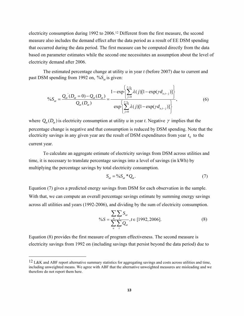
electricity consumption during 1992 to 2006.12 Different from the first measure, the second

measure also includes the demand effect after the data period as a result of EE DSM spending

that occurred during the data period. The first measure can be computed directly from the data

based on parameter estimates while the second one necessitates an assumption about the level of

electricity demand after 2006.

The estimated percentage change at utility u in year t (before 2007) due to current and past DSM spending from 1992 on, % utS is given:

0

0

,'0

,0

1 exp ( )[1 exp( )]( 0) ( )

% ,( )

exp ( )[1 exp( )]

t t

u t jjut ut ut ut

ut t tut ut

u t jj

j dQ D Q D

SQ D

j d

(6)

where ( )ut utQ D is electricity consumption at utility u in year t. Negative implies that the

percentage change is negative and that consumption is reduced by DSM spending. Note that the electricity savings in any given year are the result of DSM expenditures from year 0t to the

current year.

To calculate an aggregate estimate of electricity savings from DSM across utilities and

time, it is necessary to translate percentage savings into a level of savings (in kWh) by

multiplying the percentage savings by total electricity consumption.

% * .ut ut utS S Q (7)

Equation (7) gives a predicted energy savings from DSM for each observation in the sample.

With that, we can compute an overall percentage savings estimate by summing energy savings

across all utilities and years (1992-2006), and dividing by the sum of electricity consumption.

% , [1992, 2006].ut

u t

utu t

SS t

Q

(8)

Equation (8) provides the first measure of program effectiveness. The second measure is

electricity savings from 1992 on (including savings that persist beyond the data period) due to

12 L&K and ABF report alternative summary statistics for aggregating savings and costs across utilities and time, including unweighted means. We agree with ABF that the alternative unweighted measures are misleading and we therefore do not report them here.

14

DSM spending during 1992-2006 as a percentage over electricity consumption 1992-2006. The

difference between these two measures lies in the numerator and the common denominator permits comparison. We use the estimated and the ( )j function to predict the cumulative

percentage savings at utility u after 2006 attributable to DSM expenditures during 1992 and 2006

at that utility. The percentage saving at utility u in year k (k>2006) resulting from DSM spending

during the data period is given by:

0

0

,'0,2006 ,2006

,2006,

0

1 exp ( )[1 exp( )]( 0) ( )

% , 2006.( )

exp ( )[1 exp( )]

t t

u t jjuk u uk u

uk t tuk u

u t jj

k dQ D Q D

S kQ D

k d

(9)

,2006uD is a vector of annual DSM spending from 1992 to 2006. To predict total electricity saved

in a future year, we assume that electricity consumption is flat after 2006 for each utility.

,2006% * .uk uk uS S Q

(10)

We add these future savings to the numerator in equation (8) and obtain the second measure:

' 19922006

1992

% ,

T

utu t

utu t

SS

Q

(11)

where T is the last year when 2006 DSM spending ceases to have any demand effect. Our

estimates suggest that the effect is practically zero after 20 years so we do not add future savings

after 2026.

To examine the cost-effectiveness of DSM spending, we calculate spending (in cents) per

kWh saved. Denoting the number of customers in utility u at time t by Nut, we divide total DSM

spending across all utilities and years by total electricity savings:

2006

1992

1992

*.

ut utu t

T

utu t

d NAC

S

(12)

When the energy savings from DSM spending last a long time as our empirical results

show, one should discount future benefits in order to compare them to upfront DSM spending.

Discounting makes a bigger difference in the cost-effectiveness analysis when the energy savings

accrue over a longer time period. We calculate average cost per kWh saved (AC) using

15

alternative discount rates: 0 percent, 3 percent, 5 percent, and 7 percent. A higher discount rate

implies smaller total discounted electricity savings and hence a larger average cost estimate. We

take the estimates based on 5 percent discount rate as the focal point of discussion, as this is in

the middle of the 3 percent and 7 percent rate typically used for government policy analysis.

13

5. Estimation Variables and Data Sources

Our data set is a panel of annual utility-level data from EIA Form 861 Annual Electric

Power Industry Report and other sources over the 18-year period 1989–2006.14 The observations

in the estimation sample start in 1992 because we use DSM spending in 1989-1991 to control for

spending prior to our data period. Thus, our panel covers a period roughly twice as long as that

of L&K. Summary statistics appear in Table 1. All dollar values are converted from nominal to

real using the gross domestic product (GDP) deflator.

Our main sample has 3,326 observations from 307 utilities. The original data set from

which our main sample is drawn includes all utilities in the lower 48 states that meet the

minimum size criteria for reporting DSM expenditures throughout the sample period. We

exclude utilities with no residential customers. The original data set has many observations with

13 Recent estimates place the weighted average cost of capital for electric utilities at about 5% and the cost of equity at about 7% (Damodaran 2006).

14 Analysts have raised some concerns about the quality of the utility level data on energy efficiency collected on EIA-861, including missing values for expenditures in some years for large utilities and a lack of consistency across utilities in what gets reported for both expenditures and savings measures, particularly the annual savings (Horowitz 2004, York and Kushler 2005, Reid 2009, Horowitz 2010). Note that we do not use the EIA-861 energy savings data for our econometric analysis. Early in the course of this research, we also attempted to identify and correct shortcomings in the expenditures data, drawing on other sources including ACEEE and the Consortium for Energy Efficiency that have sought to fill in missing expenditures in certain years or collect their own data. However, we were unable to use those data because they did not have a sufficient degree of detail and time coverage necessary for our analysis. So we proceeded solely with the EIA data. Nonetheless, we did carefully check the EIA data and eliminated a number of outliers, including observations with year-to-year growth in demand or total customers in excess of 30 percent (due to mergers, acquisitions, and other factors) and utilities with no residential customers. Also, there appears to be inconsistent reporting of zeros and missing values for DSM energy efficiency expenditures in the 861 data depending on the year. We do some consistency tests across the different components of DSM expenditures to determine when reported zeros are likely missing values and when reported missing values are likely to be zeros. When energy efficiency expenditure is reported as zero and total DSM expenditures is non-zero,if the sum of the components of DSM, including energy efficiency, load management, load building (for those years when it is reported) and indirect costs, is less than the total DSM then we convert the zero expenditures to missing. Alternatively, if EE DSM is reported as missing and total DSM is reported as zero, then we treat the energy efficiency component of DSM expenditures as zero. While we believe there may be measurement error associated with the energy efficiency DSM expenditures reported to EIA, we do not believe it introduces a systematic bias to our analysis.

16

missing values for DSM spending even after our meticulous efforts to find them from various

sources.15 Because our empirical model allows all previous DSM spending to potentially affect

current demand, whenever encountering a missing DSM spending, we have to drop all

subsequent observations for the same utility.

5.1 Electricity Demand and DSM Expenditures

Data on utility-level electricity sales, DSM spending, and number of customers are from

Form EIA-861. Like L&K, we use as our measure of utility spending on energy efficiency DSM

that portion of DSM expenditures that utilities report as being devoted specifically to energy

efficiency, as opposed to load management, load building, or indirect costs.16 To be as

comprehensive as possible in our treatment of ratepayer–funded DSM energy efficiency

programs, we also include third-party state-level DSM programs that have come into being post-

restructuring.17 We share state-level third-party DSM expenditures to the utility level using each

utility’s share of total customers within the state. Given that comparisons of third-party DSM

expenditure data shared to the utility and utility-reported DSM expenditures suggest that there is

some overlap, we only include third-party expenditures in the analysis when the utility-reported

DSM expenditures are zero or missing.18 As noted in section 4, we normalized DSM

expenditures by number of customers at the utility in order to control for size. Finally, note that

conducting the analysis at the utility level means that we are able to pick up the effects of intra-

utility spillovers that would result when customers who do not participate in a program actually

15 Under Form EIA-861, utilities with sales to both ultimate consumers and resale less than 120,000 MWhwere not required to report energy efficiency expenditures through 1997. The threshold became 150,000 MWh in 1998; we therefore exclude all utilities with less than 150,000 MWh. Further, following L&K, we do not include utilities in Alaska, the District of Columbia, Hawaii, or the U.S. territories. We also drop observations that have missing values for DSM expenditures during the estimation process. 16 Note that utilities did not report expenditures for energy efficiency separately until 1992, so we use the energy efficiency share of total DSM expenditures by utility in 1992 to impute values for energy efficiency–related expenditures in prior years to use as lagged measures of energy efficiency DSM expenditures. 17 From a variety of sources, we were able to collect data on energy efficiency expenditures for third-party programs for only eight states and these data are reported in Appendix Table A-2, which shows the annual DSM expenditures by each program. When constructing these data, we did our best to match the categories of expenditures included in the energy efficiency portion of DSM spending reported by utilities to the expenditures reported by third parties, but such parsing of the third-party data into the portion that is directly comparable to the EIA definition of energy efficiency spending was not always possible. To the extent that we overrepresent the relevant category of energy efficiency spending, that would tend to bias our cost-effectiveness estimates upward.We were unable to obtain data on energy efficiency spending by the public benefit fund administrator in Ohio and thus we exclude the Ohio utilities from our estimation for the years 2000 and beyond. 18 A linear regression of utility-reported DSM expenditures on third-party DSM expenditures shared to the utility level yields a coefficient of 1, suggesting that these third-party expenditures may be incorporated into utility reports.

17

make investments in efficient equipment on their own and thus reduce their electricity

consumption at no cost to the program.

5.2 Decoupling Regulation

To test whether state-level revenue decoupling regulation leads to reduced demand, we

include a categorical variable indicating its presence.19 Because of the way electricity is priced in

most places, many of the fixed costs of delivering electricity are recovered in per-kWh charges.

This means that programs that are effective at reducing electricity consumption could also reduce

revenues that are used to recover fixed costs, potentially creating losses for the utilities that offer

DSM programs. In some states, regulators have allowed the utilities that they regulate to recover

the relevant portion of lost revenues to eliminate disincentives for offering DSM programs. One

such approach is revenue decoupling, so named because it decouples the portion of utility

revenues dedicated to recovering fixed distribution costs from the amount of electricity that the

utility sells. Note that because our data end in 2006, we do not incorporate the recent dramatic

increase in the adoption of decoupling regulation at the state level.

5.3 Building Energy Efficiency Codes

Previous studies of DSM have not examined the effects of building codes on electricity

demand.20 As a result, if building code stringency is positively correlated with average DSM

expenditures per customer,21 a portion of the energy savings caused by building codes may be

attributed to DSM spending, which would result in an underestimate of the cost per kWh

savings.22 We address this issue by including a series of categorical variables to characterize the

19 Another approach is lost revenue recovery, which allows utilities to raise prices to compensate them for revenues from sales that utilities can show were lost as a result of DSM programs. Unfortunately, data on the presence and form of state rules governing lost revenue recovery are not available for several of the years in our sample.

20Jaffe and Stavins (1995) examined the effectiveness of building codes using a cross-sectional data set, finding no significant effect of building codes on energy demand in their analysis. Aroonruengsawat et al. (2009) find that building codes decreased per capital residential electricity consumption by 3 – 5 % in 2006. Jacobsen and Kotchen (2010) find that the introduction of more stringent building codes in Gainesville, Florida reduced demand for electricity by about 4%. Costa and Kahn (2009) find that building codes affect residential electricity consumption in California after 1983 but not before. 21 In our sample, we find a small positive correlation of building code stringency and DSM expenditures per customer. 22 In some cases, however, such attribution may not be so far off. A significant issue with building codes is compliance, and for some utilities in some years, a portion of DSM expenditures may be devoted to improving compliance with residential building codes. In these cases DSM could increase the potential for building codes to yield savings.

18

stringency of building codes within each state during each year. We obtained data on the

evolution of energy building codes from the Building Codes Assistance Project (www.bcap-

energy.org) and the DOE Building Energy Codes Program (www.energycodes.gov). See Figure

2 for a map of building code stringency as of 2007, which shows the western states, such as

California and Washington, with the most stringent building codes and Midwestern states with

typically less stringent codes.

We began by creating six categories of building code stringency, which, in order of

decreasing stringency, are: (a) code met or exceeded the 2006 International Energy Conservation

Code (IECC) or equivalent and was mandatory statewide; (b) code met 2003 IECC or equivalent

and was mandatory statewide; (c) code met the 1998–2001 IECC or equivalent and was

mandatory statewide; (d) code preceded the 1998 IECC or equivalent and was mandatory

statewide; (e) significant adoptions in jurisdictions, but not mandatory statewide; and (f) none of

the aforementioned conditions hold and no significant adoptions of building codes in the state.

After speaking with a building codes expert, we further consolidated these into four categories to

represent more substantial differences in stringency: BC1 indicates the stringency is (a) above;

BC2indicates the stringency is (a)–(d) above; BC3 indicates the stringency is (a)–(e) above; the

fourth (excluded) category is category (f).23 Thus, the variables are structured to indicate the

incremental effect of building codes compared to the next most-stringent category.

5.4 Energy Prices and Other Variables

The annual average price of electricity by state also comes from Form EIA-861.24

Residential natural gas and fuel oil prices by state also come from EIA. We compiled state-level

data on several other variables from a variety of sources. Annual state-level GDP comes from the

Bureau of Economic Analysis. Data on population-weighted heating and cooling degree days by

state are from the National Oceanic and Atmospheric Administration (NOAA).These data are

23 We also obtained data on energy efficiency codes for commercial buildings. However, we found a high correlation between the residential and commercial building code stringency, and so chose to focus on a single measure of stringency. 24 Electricity prices can vary substantially across utlities within a state and our price data will not reflect this intra-state variation in price levels where it exists However, given the potential for endogeneity introduced by using utlity level price data, and the fact that our analysis focuses on changes in price and not price levels, we believe that using state level prices for electricity and other fuels is appropriate.

19

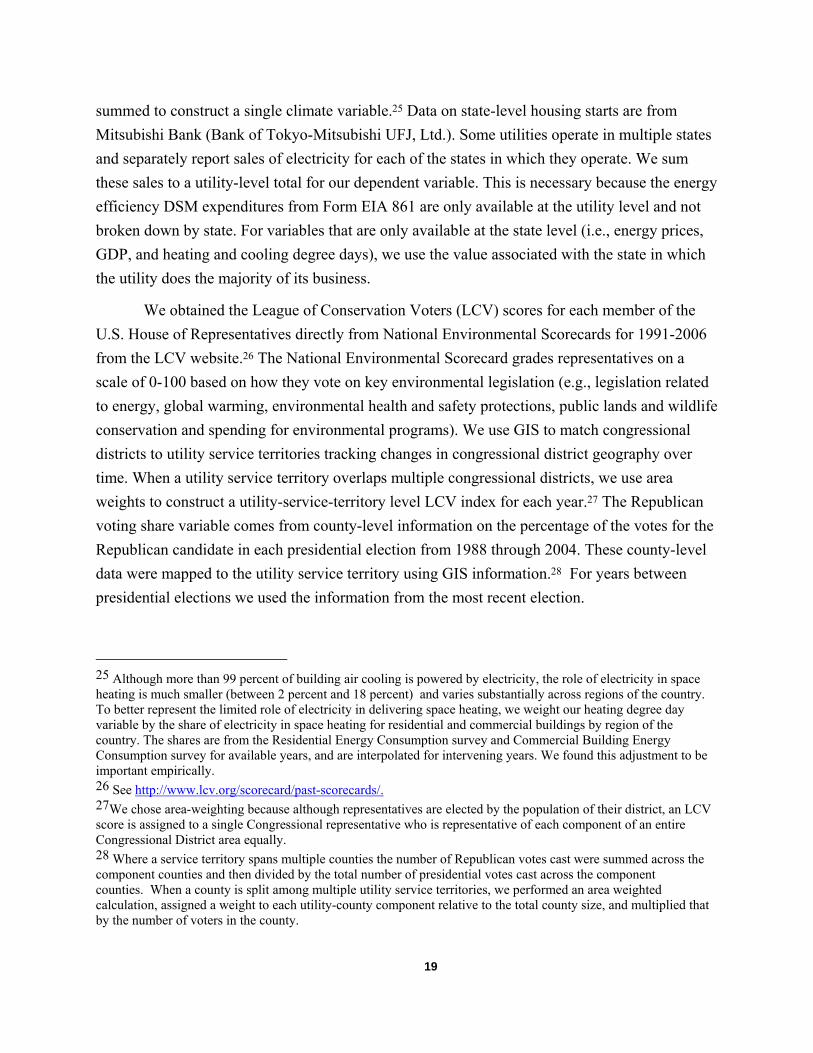
summed to construct a single climate variable.25 Data on state-level housing starts are from

Mitsubishi Bank (Bank of Tokyo-Mitsubishi UFJ, Ltd.). Some utilities operate in multiple states

and separately report sales of electricity for each of the states in which they operate. We sum

these sales to a utility-level total for our dependent variable. This is necessary because the energy

efficiency DSM expenditures from Form EIA 861 are only available at the utility level and not

broken down by state. For variables that are only available at the state level (i.e., energy prices,

GDP, and heating and cooling degree days), we use the value associated with the state in which

the utility does the majority of its business.

We obtained the League of Conservation Voters (LCV) scores for each member of the

U.S. House of Representatives directly from National Environmental Scorecards for 1991-2006

from the LCV website.26 The National Environmental Scorecard grades representatives on a

scale of 0-100 based on how they vote on key environmental legislation (e.g., legislation related

to energy, global warming, environmental health and safety protections, public lands and wildlife

conservation and spending for environmental programs). We use GIS to match congressional

districts to utility service territories tracking changes in congressional district geography over

time. When a utility service territory overlaps multiple congressional districts, we use area

weights to construct a utility-service-territory level LCV index for each year.27 The Republican

voting share variable comes from county-level information on the percentage of the votes for the

Republican candidate in each presidential election from 1988 through 2004. These county-level

data were mapped to the utility service territory using GIS information.28 For years between

presidential elections we used the information from the most recent election.

25 Although more than 99 percent of building air cooling is powered by electricity, the role of electricity in space heating is much smaller (between 2 percent and 18 percent) and varies substantially across regions of the country. To better represent the limited role of electricity in delivering space heating, we weight our heating degree day variable by the share of electricity in space heating for residential and commercial buildings by region of the country. The shares are from the Residential Energy Consumption survey and Commercial Building Energy Consumption survey for available years, and are interpolated for intervening years. We found this adjustment to be important empirically. 26 See http://www.lcv.org/scorecard/past-scorecards/. 27We chose area-weighting because although representatives are elected by the population of their district, an LCV score is assigned to a single Congressional representative who is representative of each component of an entire Congressional District area equally. 28 Where a service territory spans multiple counties the number of Republican votes cast were summed across the component counties and then divided by the total number of presidential votes cast across the component counties. When a county is split among multiple utility service territories, we performed an area weighted calculation, assigned a weight to each utility-county component relative to the total county size, and multiplied that by the number of voters in the county.

20

6. Estimation and Results

We first estimate equation (5) using nonlinear least squares assuming no endogeneity in

DSM spending, as has been done in previous studies in this literature. To address the issue of

possible endogeneity, we then estimate equation (5) using nonlinear GMM as discussed in

section 4. A variety of robustness checks are conducted to check the sensitivity of the findings

with respect to assumptions on demand specification, parametric assumptions on the time path

the effects of past DSM spending, treatment of missing DSM data, as well as controlling for

DSM spending before 1992. Based on the estimated parameters, we examine the effectiveness

and cost-effectiveness of DSM spending. The results appear in Tables 2-6. In the following, we

first present coefficient estimates and we then discuss their implications for program

effectiveness and cost-effectiveness.

6.1 Coefficient Estimates

Table 2 presents coefficient estimates and their standard errors from estimating equation

(5). The first-difference equation includes year dummies and the control function to capture the

demand effect of EE DSM spending before 1992. As discussed in Section 4.1, the control

function includes nine interaction terms between the polynomials of the average level of DSM

spending during 1989-1991 and the polynomials of the time trend variable.29 The results under

model 1 are obtained from nonlinear least squares (NLS). The results under model 2 are from

GMM where we use the polynomials (up to 5th order) of the lagged spending (the 4th lags and those earlier) to construct the optimal instrument , 1[log( / ) | , ]ut u tE Q Q z as described in

Section 4.2. Model 3 includes LCV scores and percentage of Republican presidential votes in the

last election in each utility service territory as additional variables to construct optimal

instruments.

The parameter estimates across the three models are very close, suggesting that current

DSM spending is not correlated with current demand shocks. This similarity may reflect that

DSM spending is determined before the current demand shocks are realized. If utilities base their

DSM spending on (projected) future demand conditions, their predictions of future demand

conditions can be captured well by the observed demand factors used in our model. Basing

current DSM spending on expectations regarding future demand growth is consistent with an

integrated planning model approach in which utilities see energy efficiency investments as an

29 These nine interactions are

2 3 2 3 2 32 2 2 3 3 3* , * , * , * , * , * , * , * , *d d d d d d d d d .

21

alternative to building new power plants in order to balance demand and supply in the future

(Gillingham et al. 2006). This finding also holds in other demand specifications to be discussed

in the next section. In all of the models, we find a negative estimate for the γ coefficient. Given that ( )j in equation (4) is always positive, a negative γ implies a negative relationship between

electricity demand and DSM spending per customer. The magnitude of the γ coefficient, which

gives the rate at which diminishing returns set in, is quite small, implying that the diminishing

return is not strong at least for the spending levels observed in the data. Since our model is

nonlinear in parameters, the demand effect of DSM spending is determined by γ and other

parameters in the model.

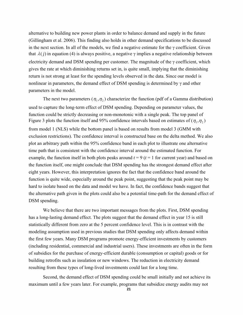
The next two parameters ( 1 2, ) characterize the function (pdf of a Gamma distribution)

used to capture the long-term effect of DSM spending. Depending on parameter values, the

function could be strictly decreasing or non-monotonic with a single peak. The top panel of Figure 3 plots the function itself and 95% confidence intervals based on estimates of ( 1 2, )

from model 1 (NLS) while the bottom panel is based on results from model 3 (GMM with

exclusion restrictions). The confidence interval is constructed base on the delta method. We also

plot an arbitrary path within the 95% confidence band in each plot to illustrate one alternative

time path that is consistent with the confidence interval around the estimated function. For

example, the function itself in both plots peaks around t = 9 (t = 1 for current year) and based on

the function itself, one might conclude that DSM spending has the strongest demand effect after

eight years. However, this interpretation ignores the fact that the confidence band around the

function is quite wide, especially around the peak point, suggesting that the peak point may be

hard to isolate based on the data and model we have. In fact, the confidence bands suggest that

the alternative path given in the plots could also be a potential time-path for the demand effect of

DSM spending.

We believe that there are two important messages from the plots. First, DSM spending

has a long-lasting demand effect. The plots suggest that the demand effect in year 15 is still

statistically different from zero at the 5 percent confidence level. This is in contrast with the

modeling assumption used in previous studies that DSM spending only affects demand within

the first few years. Many DSM programs promote energy-efficient investments by customers

(including residential, commercial and industrial users). These investments are often in the form

of subsidies for the purchase of energy-efficient durable (consumption or capital) goods or for

building retrofits such as insulation or new windows. The reduction in electricity demand

resulting from these types of long-lived investments could last for a long time.

Second, the demand effect of DSM spending could be small initially and not achieve its

maximum until a few years later. For example, programs that subsidize energy audits may not

22

see immediate results as it may take time for customers to take up all the recommendations from

these programs (e.g., making energy-efficient investments). To the extent that these

recommendations could require a large financial commitment, consumers may not act upon them

immediately. This may be especially true for industrial and commercial customers if the

investment involves significant capital turnover. Also, according to Gillingham et al. (2004), by

the 1990s utilities were increasingly focusing their DSM spending on market transformation

programs that sought to transform markets for energy using equipment such that the efficient

option becomes the norm. These types of programs involved coordinated information, training,

demonstration and financing campaigns and their effectiveness could very well build over time

as suggested by our results. While it is impossible to know from our EE DSM expenditure data

exactly what types of programs utilities were funding during the years for which we have data,

our results are consistent with some of the general trends in program evolution identified by

Gillingham et al. (2004).

The remaining parameter estimates are intuitively signed and in most cases are

statistically significant. The relationships between electricity demand and indicators of the size

of the market (number of customers and population) and overall economic condition (gross state

product and housing starts) are positive and significant across the different models. We include

prices of electricity, natural gas and fuel oil (in logarithm) and their quadratic terms to allow for

more flexible elasticity patterns. Electricity demand is significantly negatively associated with

the price of electricity (elasticity of -0.27 at the mean level of electricity price), and is positively

associated with the prices of natural gas and fuel oil (elasticity of 0.04 and 0.18 at the mean level

of prices).30 Electricity demand is also positively associated with increases in the climate variable

(i.e., heating/cooling degree days) and the size of this effect is fairly consistent across the

different models at an elasticity of about 0.1. In all models, we also include building code

stringency dummies (base group: no building codes) and their interactions with housing starts.

Recall from section 5 that the dummy for having building codes is one if there is any type of

building codes in the area (regardless of stringency) while the two dummies for more stringent

building codes are one for all areas that have building codes above a certain threshold. The

30 The parameter estimates on electricity price suffer from the potential endogeneity problem and is better interpreted as an indication of association rather than causation.

23

coefficient estimates suggests that having the most stringent building codes reduces electricity

demand and the reduction effect is stronger in areas with more housing starts.31

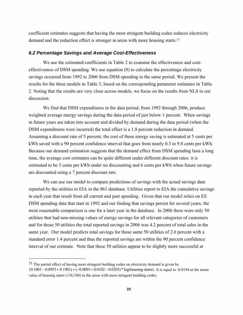
6.2 Percentage Savings and Average Cost-Effectiveness

We use the estimated coefficients in Table 2 to examine the effectiveness and cost-

effectiveness of DSM spending. We use equation (8) to calculate the percentage electricity

savings occurred from 1992 to 2006 from DSM spending in the same period. We present the

results for the three models in Table 3, based on the corresponding parameter estimates in Table

2. Noting that the results are very close across models, we focus on the results from NLS in our

discussion.

We find that DSM expenditures in the data period, from 1992 through 2006, produce

weighted average energy savings during the data period of just below 1 percent. When savings

in future years are taken into account and divided by demand during the data period (when the

DSM expenditures were incurred) the total effect is a 1.8 percent reduction in demand.

Assuming a discount rate of 5 percent, the cost of these energy saving is estimated at 5 cents per

kWh saved with a 90 percent confidence interval that goes from nearly 0.3 to 9.8 cents per kWh.

Because our demand estimation suggests that the demand effect from DSM spending lasts a long

time, the average cost estimates can be quite different under different discount rates: it is

estimated to be 3 cents per kWh under no discounting and 6 cents per kWh when future savings

are discounted using a 7 percent discount rate.

We can use our model to compare predictions of savings with the actual savings data

reported by the utilities to EIA in the 861 database. Utilities report to EIA the cumulative savings

in each year that result from all current and past spending. Given that our model relies on EE

DSM spending data that start in 1992 and our finding that savings persist for several years, the

most reasonable comparison is one for a later year in the database. In 2006 there were only 50

utilities that had non-missing values of energy savings for all relevant categories of customers

and for those 50 utilities the total reported savings in 2006 was 4.2 percent of total sales in the

same year. Our model predicts total savings for those same 50 utilities of 2.6 percent with a

standard error 1.4 percent and thus the reported savings are within the 90 percent confidence

interval of our estimate. Note that these 50 utilities appear to be slightly more successful at

31 The partial effect of having most stringent building codes on electricity demand is given by (0.1061 0.0953 0.1981) ( 0.0091 0.0102 0.0203)*log(housing starts) . It is equal to -0.0184 at the mean

value of housing starts (138,340) in the areas with most stringent building codes.

24

producing savings as the average cumulative savings in 2006 for all 126 utilities in our data set is

only 2.1 percent with a standard error of 1.1 percent.

The expected average cost estimate of 5 cents per kWh for utility costs is less than the

national average retail price of electricity in 2006 of 9.1 cents per kWh across all sectors (EIA

2009). Recall, however, that these are costs only for the utility itself. The fact that the average

electricity price is higher than the estimated utility cost per kWh saved suggests that these

programs may have produced zero-cost or low-cost CO2 emissions reductions, depending on the

magnitude of the costs to utility customers of implementing energy efficiency measures.

Although the marginal cost of electricity—which is not generally equal to the electricity price—

is perhaps a better estimate of the benefits of energy savings from DSM, estimates of marginal

cost can vary substantially depending on what margin is being considered. In the short run, the

marginal cost of generation can vary substantially by time of day. For example, in December

2006, the hourly marginal cost of generation ranged from roughly 2 cents per kWh to 27 cents

per kWh depending on location and time of day (PJM 2006). In the longer run, marginal

generation costs are given by the levelized cost of new investments, which vary by technology

and fuel and, according to the National Academy of Sciences (2009), range from roughly 8–9

cents per kWh for new baseload fossil capacity to a little over 13 cents per kWh for a new gas

turbine peaker.

Accounting for customer costs is also challenging. Earlier research (Nadel and Geller

1996; Joskow and Marron 1992) suggests that the sum of customer costs and utility costs is

roughly 1.7 times utility costs alone. Because this ratio is based on such a small number of

somewhat dated studies, we do not think it is appropriate to use this ratio to estimate customer

costs for our results. Nonetheless, it suggests that the total average cost of a kWh saved is still

below the price of electricity, suggesting that energy efficiency programs can be a cost-effective

way to reduce CO2 emissions.

Our estimate is in the range of some more recent estimates of the cost-effectiveness of

energy efficiency programs. For example, PG&E (2010) finds that its energy efficiency

programs in 2009 produced savings at an average cost to the utility of 4.5 cents per kWh saved.

6.3 Robustness Analysis

To check the sensitivity of our findings to modeling assumptions, we conduct a variety of

robustness checks. The first robustness check is with respect to the specification of the model.

The baseline specification given by equation (4) assumes that DSM spending enters the demand

equation nonlinearly, which is to capture the possibility that the demand reduction effect could

25

have a diminishing return. In an alternative specification, we let the DSM spending variable

enter the demand equation linearly:

(13) 0

0, 1,0

ln( ) ( ) ( , ) .t t

u tut ut u t u t j t utj

Q X j d f d

The estimation results based on NLS and GMM with exclusion restrictions for this

specification are presented in Table 4. NLS and GMM results are very similar to the baseline

specification, again suggesting that DSM spending is not correlated with idiosyncratic demand

shocks. The parameter estimates from this alternative specification are very close to those from the baseline specification shown in Table 2. This is consistent with the fact that is estimated to

be very close to zero in the baseline specification, implying a near linear relationship between

DSM variables and the dependent variable. The percentage electricity savings and average cost

estimates from the alternative specification, shown in panel 1 in Table 6, are also similar to those

in the baseline specification. The average cost per kWh saved is estimated to be 4.8 cents with a

discount rate of 5 percent, compared to 5.0 cents in the baseline specification.

The second robustness check is with respect to missing data in the sample. Because we

have to drop all the observations subsequent to a missing one for the same utility, this implies

that the number of utilities used in the analysis is smaller over time. To check how this could

affect estimation results, we use the same demand function specification as the baseline but focus

on utilities that have at least 10 observations in the data and this gives rise to 3,014 instead of

3,326 observations. The parameter estimates are close to those in the baseline model. Panel 2 of

Table 6 provides the estimates of percentage electricity savings and average cost, all of which are

similar to the baseline estimates as well.

In the third robustness check, we investigate the sensitivity of the findings to the control

function used to capture the demand effect of DSM spending occurred before 1989, the first year

of our data. Recall that we use a polynomial function of average DSM spending between 1989

and 1991 and the time trend as the control function. The baseline specification includes

interaction terms between 3rd-degree polynomials of the average annual level of DSM spending

during 1989-1991 and those of the time trend variable (9 interactions in total)) while in this

robustness check, we include interaction terms of 4th-degree polynomials of each of the two

variables (16 interactions). Estimation results from this specification, shown in the first part of

26

Table 5 and the third panel of Table 6, are still in line with those in the baseline model.32 The

fourth alternative specification employs a different parameter function to capture the long-term

demand effect of DSM spending. Instead of the probability density function of the Gamma

distribution in the baseline model, we use a Weibull distribution which is also a two-parameter

function and allows flexible pattern of the time path. The parameter estimates are presented in Table 5. Based on the estimates for 1 2, , we plot the function and the 95% confidence interval

in Figure 4. The two plots correspond to estimation results from NLS and GMM with exclusion

restriction. The two salient features observed in Figure 3 for the baseline specification are still

present in Figure 4: DSM spending could have a long-lasting effect and the effect could be small

initially and reach its maximal strength a few years later. Panel 4 of Table 6 shows the

percentage saving and average cost estimates. The average cost decreases from 5 cents in the

baseline to 4 cents in this specification. Nevertheless, given the standard errors for these two

estimates, the difference would not be statistically significant.

The specific nature of the individual EE DSM activities included in these utility and state

programs is not discernible in our data, and there can be substantial variability across programs.

While some DSM programs are implemented with a direct goal of reducing consumption within

utility service territories, others are carried out as less intensive pilot programs or customer

service activities (e.g., information programs).33 If one expects that the programs under the

second category have a smaller effect on energy saving (per dollar of expenditure), our results

from combining all types of programs together would under-estimate the effect of demand

reduction from the programs in the first category (i.e., more intensive programs explicitly

motivated to achieve high energy savings).

To examine this issue, we conduct two additional robustness checks where we drop “less

committed” utilities that have positive DSM spending but whose spending per customer is below

the 10th percentile or the 20th percentile of the DSM spending distribution (among the utilities

who carried out DSM spending). The results from these two robustness checks are very similar

to those obtained for the baseline model, and are available upon request. For example, demand

reduction from DSM spending during the data period is -0.92% from Model 1 (NLS in Table 2)

32We note that we also estimate the model without including the control function. Because this approach would attribute the demand effect of DSM spending that occurred before 1992 to expenditures in later years, the results show that the demand effect would be substantially overestimated: the estimated percentage savings during 1992-2006 is 3.2 percent and the cost per kWh saved is less than one cent compared to 0.9 percent and five cents in the baseline model. 33 We thank one of the referees for calling this issue to our attention.

27

while the effect is estimated at -0.93% in the first robustness check and -0.89% in the second

robustness check, all being significant at the 10% level. The central cost-effectiveness estimate

from these more limited samples actually increases somewhat, although the change is not

statistically significant from the baseline model. This is also consistent with the fact that in the baseline model, (the rate of diminishing returns) is estimated to be very close to zero in the

baseline specification, implying a near linear relationship between DSM per customer and

log(electricity consumption) for the data we have.

To investigate whether revenue decoupling strengthens the demand-reducing effect of

DSM spending, we add an interaction term between DSM spending and the decoupling dummy

in the baseline specification. The demand equation becomes:

(15) 0

0, 11 , 2 , ,0

ln( ) ( )[1 exp( decoup )] ( , ) .t t

u tut ut u t u t j u t j u t j t utj

Q X j d d f d

Decoup is a dummy variable equal to 1 if revenue decoupling policy is in effect for the utility. The estimates for 1 2 and from NLS are -0.0006 (0.0007) and -0.0034 (0.0029) with standard

errors in parenthesis. The 2 estimate suggests that the demand reduction effect is stronger

among utilities that have revenue decoupling regulation. However, it is not statistically

significant, likely due to the fact that only 7 percent of the observations are affected by this

policy and the policy status does not change often over time for the same utility during our data

period (more and more utilities are subject to this policy after 2006, the end of our data period).

All the other parameter estimates (not reported to save space) are close to those in the baseline

model. Moreover, NLS and GMM give similar results as well. The percentage savings estimates

based on equations (8) and (11) are 0.9 percent (0.5) and 1.5 percent (1.0) from NLS. The

average cost per kWh saved is 6 cents with a standard error of 4 with a discount rate of 5 percent.

7. Conclusion

The cost-effectiveness of utility DSM programs is a subject of considerable interest and

study. Most of the past efforts to study cost-effectiveness take utility reports of electricity

savings attributable to DSM programs as given, often adjusting by a pre-established net-to-gross

factor to account for free riders net of spillover effects. In this analysis, we take a different

approach that relies on econometric techniques to estimate how DSM expenditures affect

electricity demand, controlling for other demand drivers, such as changes in price, income and

weather. We build on earlier work by expanding the dataset and including additional important

explanatory variables. More importantly, we develop a carefully motivated empirical model to

capture the long-term demand effect of DSM expenditure. We explicitly address the potential

28

endogeneity problem of DSM expenditure using nonlinear GMM, which has not been done

previously.

Our main results suggest that, over the 15-year period covered by this analysis,

ratepayer–funded DSM expenditures produced a central estimate of 0.9 percent savings in

electricity consumption within the data period and 1.8 percent savings including savings that

occur beyond the data period. The average cost to utilities of electricity savings achieved under

these programs depends importantly on the discount rate employed to calculate the present

discounted value of future electricity savings. With a discount rate of 5 percent, the average cost

is 5 cents per kWh saved, with a 90 percent confidence interval that goes from 0.3 cents to nearly

10 cents per kWh saved. Higher discount rates yield higher mean estimates of average cost. Our

findings are robust to many alternative assumptions about model structure and the structural

model used to incorporate the effects of lagged DSM spending. Our model suggests that over the

range of DSM spending data in our sample, returns to increased EE DSM spending are roughly

constant. Decoupling regulation appears to strengthen the demand-reducing effects of EE DSM

spending. Our results do provide evidence that for utilities primarily located in states where

housing starts are above the mean, the presence of more stringent building costs has a

statistically significant negative effect on electricity demand.

In future work, it would be useful to discern lessons about the relative effectiveness of

different types of energy efficiency programs (e.g. information programs versus rebate programs

versus loan programs) or the relative effectiveness of programs targeted at different classes of

customers (residential, commercial, industrial), both of which would require more detailed data

on EE DSM spending by program type and type of customer. In recent years energy efficiency

regulatory policy has focused on questions of who is best suited to deliver energy savings

through efficiency investments at the point of use and what types of regulatory incentives are

necessary to encourage utilities to embrace end-use energy efficiency. States have opted either to

charge the electric utilities with promoting energy efficiency or have chosen to establish a

separate state-run or state-chartered entity (e.g., Efficiency Maine Trust, Efficiency Vermont or

NYSERDA) to operate its ratepayer funded energy efficiency programs.

On the regulatory side, state utility regulators have had a renewed interest in developing

regulatory mechanisms such as revenue decoupling and incentive mechanisms to reward

successful energy efficiency programs to help overcome utility incentives to maximize revenues

and profits through greater electricity sales. As experience with these different structural and

regulatory institutions accumulates, we hope the necessary data will be collected to enable us and

other researchers to identify the implications of these different institutional arrangements and

29

regulatory approaches for the performance of programs that use ratepayer funds and other public

dollars to invest in greater end-use energy efficiency.

Utility energy efficiency programs are taking center stage in ongoing discussions about

U.S. energy policy and how best to combat climate change. Studies such as the recent McKinsey

Study (Granade et al. 2009) on the potential for saving energy at low or negative cost are part of

this debate. However, missing from studies like McKinsey’s are the specific policy measures that

would be required to bring about the investments and behavioral changes necessary to realize

these energy savings and estimates of the extent to which the costs of implementing these

policies might differ from the engineering costs. The present study offers additional evidence

about how effective past utility and third-party state-level programs have been in reducing

electricity demand, and how much they have cost per unit of electricity saved.

30

Table 1: Summary Statistics

Variables Mean Median Std. Dev. Min Max

First difference of Log(electricity demand) 0.031 0.028 0.045 -0.290 0.297

Electricity demand (billion KWH) 7.98 1.08 16.02 0.16 103.65

Electricity demand per customer (MWH) 24.02 21.49 10.75 8.21 96.52

DSM spending ($ millions) 4.71 0.06 16.82 0.00 230.20

DSM spending per customer ($) 9.41 1.19 18.08 0.00 191.85

Number of customers (thousands) 325 53 678 4 5,121

Population (thousands) 9,139 6,452 8,072 574 36,200

State GDP ($ billions) 362 256 346 18 1788

Housing starts (thousands) 48 31 52 2 265

Electricity price (cents per KWH) 8.80 8.12 2.37 4.90 15.87

Natural gas price (cents per Mcf) 10.30 9.79 2.91 5.35 22.12

Fuel oil price (cents per gallon) 130.43 119.49 35.84 73.40 275.31

Climate 1,647 1,454 825 369 3,937

Indicator: most stringent building codes 0.028 0.000 0.165 0.000 1.000

Indicator: more stringent building codes 0.797 1.000 0.402 0.000 1.000

Indicator: building codes exist 0.852 1.000 0.355 0.000 1.000

Mean DSM spending per customer 89-91 ($) 7.40 0.81 13.18 0.00 64.82

Number of observations 3,326

Number of utilities 307

Notes: Dollars are inflation-adjusted to 2007. Mcf denotes thousand cubic feet.

31

Table 2: Estimation Results from the Baseline Model

Variables Model 1: NLS Model 2: GMM Model 3: GMMPara. S.E. Para. S.E. Para. S.E.

DSM spending per customer -0.0016 0.0010 -0.0015 0.0010 -0.0016 0.0010

in Gamma probability density function 8.4155 5.7705 8.8819 6.1876 8.3271 5.7275

in Gamma probability density function 0.7768 0.5972 0.8282 0.6409 0.7672 0.5930

Log(number of customers) 0.3617 0.0453 0.3617 0.0454 0.3617 0.0454

Log(population) 0.4573 0.0921 0.4574 0.0921 0.4573 0.0921

Log(gross state product) 0.2003 0.0436 0.2004 0.0436 0.2002 0.0436

Log(house starts) 0.0381 0.0080 0.0381 0.0080 0.0381 0.0080

Log(electricity price) -0.4660 0.1905 -0.4655 0.1908 -0.4661 0.1909

Log(electricity price) squared 0.0911 0.0406 0.0910 0.0407 0.0911 0.0407

Log(natural gas price) 0.1229 0.0589 0.1228 0.0588 0.1229 0.0589

Log(natural gas price) squared -0.0349 0.0143 -0.0349 0.0143 -0.0349 0.0143

Log(fuel oil price) 0.3451 0.2213 0.3460 0.2213 0.3449 0.2212

Log(fuel oil price) squared -0.0344 0.0232 -0.0345 0.0232 -0.0344 0.0232

Log(climate) 0.0962 0.0066 0.0962 0.0066 0.0962 0.0066

Dummy for most stringent bldg codes 0.1061 0.0586 0.1054 0.0586 0.1062 0.0586

Dummy for more stringent bldg codes -0.0953 0.0928 -0.0953 0.0928 -0.0953 0.0928

Dummy for bldg codes exist 0.1981 0.0861 0.1982 0.0861 0.1981 0.0861

Log(house starts)*most stringent codes -0.0091 0.0050 -0.0091 0.0050 -0.0091 0.0050

Log(house starts)*more stringent codes 0.0102 0.0093 0.0102 0.0093 0.0102 0.0093

Log(house start)*existing codes -0.0203 0.0086 -0.0203 0.0086 -0.0203 0.0086

Year dummies (14) Yes Yes Yes

Control function for early DSM Yes Yes Yes

Notes: The number of observations is 3,326. Results are for equation (4). The dependent variable is log(electricity demand). The first set of results is from NLS while the second and third sets are from GMM using optimal instruments in an iterative procedure. Model 2 does not include exclusion restrictions in constructing optimal instruments while model 3 includes LCV scores as well as the percentage of Republican votes in each utility’s service area in the last presidential election. Parameter estimates in bold are significant at the 10% level.

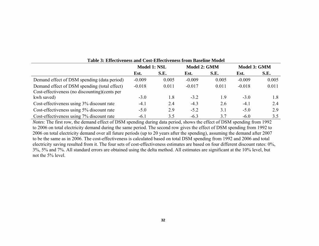
32

Table 3: Effectiveness and Cost-Effectiveness from Baseline Model Model 1: NSL Model 2: GMM Model 3: GMM Est. S.E. Est. S.E. Est. S.E. Demand effect of DSM spending (data period) -0.009 0.005 -0.009 0.005 -0.009 0.005Demand effect of DSM spending (total effect) -0.018 0.011 -0.017 0.011 -0.018 0.011Cost-effectiveness (no discounting)(cents per kwh saved) -3.0 1.8 -3.2 1.9 -3.0 1.8Cost-effectiveness using 3% discount rate -4.1 2.4 -4.3 2.6 -4.1 2.4Cost-effectiveness using 5% discount rate -5.0 2.9 -5.2 3.1 -5.0 2.9Cost-effectiveness using 7% discount rate -6.1 3.5 -6.3 3.7 -6.0 3.5Notes: The first row, the demand effect of DSM spending during data period, shows the effect of DSM spending from 1992 to 2006 on total electricity demand during the same period. The second row gives the effect of DSM spending from 1992 to 2006 on total electricity demand over all future periods (up to 20 years after the spending), assuming the demand after 2007 to be the same as in 2006. The cost-effectiveness is calculated based on total DSM spending from 1992 and 2006 and total electricity saving resulted from it. The four sets of cost-effectiveness estimates are based on four different discount rates: 0%, 3%, 5% and 7%. All standard errors are obtained using the delta method. All estimates are significant at the 10% level, but not the 5% level.

33

Table 4: Robustness Checks: First Two Sets

Robustness 1: log-linear specification Robustness 2: a subsample

NSL GMM NLS GMM

Variables Para S.E. Para S.E. Para S.E. Para S.E.

DSM spending per customer -0.0016 0.0009 -0.0016 0.0009 -0.0015 0.0010 -0.0014 0.0010

in Gamma pdf 7.7790 5.0811 7.7955 5.1572 8.5685 6.0393 8.9962 6.4233

in Gamma pdf 0.7000 0.5244 0.7019 0.5325 0.8000 0.6290 0.8473 0.6695Log(number of customers) 0.3617 0.0454 0.3617 0.0454 0.3916 0.0519 0.3916 0.0519Log(population) 0.4571 0.0920 0.4571 0.0920 0.4435 0.0964 0.4436 0.0964Log(gross state product) 0.2001 0.0436 0.2001 0.0436 0.1991 0.0463 0.1993 0.0462Log(house starts) 0.0381 0.0080 0.0381 0.0081 0.0330 0.0086 0.0330 0.0086Log(electricity price) -0.4665 0.1905 -0.4665 0.1909 -0.4896 0.1937 -0.4893 0.1940Log(electricity price) squared 0.0912 0.0406 0.0912 0.0407 0.0953 0.0413 0.0952 0.0413Log(natural gas price) 0.1231 0.0589 0.1231 0.0589 0.1134 0.0603 0.1133 0.0603Log(natural gas price) squared -0.0350 0.0143 -0.0350 0.0143 -0.0318 0.0147 -0.0317 0.0147Log(fuel oil price) 0.3430 0.2212 0.3430 0.2212 0.3303 0.2260 0.3312 0.2260Log(fuel oil price) squared -0.0342 0.0232 -0.0342 0.0232 -0.0332 0.0237 -0.0333 0.0237Log(climate) 0.0962 0.0066 0.0962 0.0066 0.1031 0.0069 0.1031 0.0069Dummy for most stringent bldg codes 0.1076 0.0585 0.1075 0.0585 0.1000 0.0590 0.0994 0.0590Dummy for more stringent bldg codes -0.0952 0.0929 -0.0952 0.0929 -0.0891 0.0927 -0.0891 0.0926Dummy for bldg codes exist 0.1981 0.0862 0.1981 0.0861 0.1961 0.0859 0.1962 0.0859Log(house starts)*most stringent codes -0.0093 0.0050 -0.0093 0.0050 -0.0085 0.0050 -0.0085 0.0050Log(house starts)*more stringent codes 0.0102 0.0093 0.0102 0.0093 0.0097 0.0093 0.0097 0.0093Log(house start)*existing codes -0.0203 0.0086 -0.0203 0.0086 -0.0201 0.0086 -0.0201 0.0086Year dummies (14) Yes Yes Yes YesControl function for early DSM Yes Yes Yes YesNotes: the first set of robustness checks is based on equation (13) which assumes that DSM spending enters the demand equation linearly. The second set of estimations is based on utilities that have at least 10 observations in the data (3,014 observations in total). GMM estimations in both sets include exclusion restrictions (LCV and percentage Republican votes) in constructing the optimal instruments.

34

Table 5: Additional Robustness Checks

Robustness 3: different control function Robustness 4: Weibull distribution

NSL GMM NLS GMM

Variables Para S.E. Para S.E. Para S.E. Para S.E.

DSM spending per customer -0.0018 0.0012 -0.0018 0.0011 -0.002 0.0012 -0.002 0.0014

in pdf 7.8165 5.1638 8.2783 5.3018 12.3169 2.3712 12.3756 2.4461

in pdf 0.6926 0.5245 0.7449 0.5398 2.8819 1.1952 2.8605 1.3109Log(number of customers) 0.3615 0.0455 0.3591 0.0454 0.3617 0.0455 0.3617 0.0455Log(population) 0.4626 0.0928 0.4589 0.0929 0.4576 0.0919 0.4575 0.092Log(gross state product) 0.2019 0.0438 0.2022 0.0438 0.198 0.0435 0.198 0.0434Log(house starts) 0.0385 0.0081 0.0382 0.0081 0.0382 0.0081 0.0383 0.0081Log(electricity price) -0.4658 0.1915 -0.4492 0.1919 -0.4647 0.1912 -0.4647 0.1919Log(electricity price) squared 0.0912 0.0408 0.0873 0.0409 0.091 0.0408 0.0911 0.041Log(natural gas price) 0.1248 0.0589 0.128 0.0588 0.1245 0.0589 0.1246 0.0589Log(natural gas price) squared -0.0354 0.0143 -0.0362 0.0143 -0.0353 0.0143 -0.0354 0.0143Log(fuel oil price) 0.3359 0.2212 0.3227 0.2214 0.3332 0.2208 0.3325 0.2208Log(fuel oil price) squared -0.0334 0.0232 -0.032 0.0232 -0.0331 0.0231 -0.033 0.0231Log(climate) 0.0961 0.0066 0.0954 0.0066 0.0962 0.0066 0.0962 0.0066Dummy for most stringent bldg codes 0.1071 0.0578 0.1111 0.0579 0.1124 0.0582 0.1127 0.0581Dummy for more stringent bldg codes -0.0925 0.0933 -0.0931 0.0931 -0.0951 0.0934 -0.0951 0.0935Dummy for bldg codes exist 0.1964 0.0863 0.1979 0.0862 0.1982 0.0864 0.1982 0.0864Log(house starts)*most stringent codes -0.0092 0.0049 -0.0096 0.0049 -0.0097 0.0049 -0.0097 0.0049Log(house starts)*more stringent codes 0.01 0.0094 0.01 0.0094 0.0102 0.0094 0.0102 0.0094Log(house start)*existing codes -0.0202 0.0087 -0.0203 0.0087 -0.0204 0.0087 -0.0204 0.0087Year dummies (14) Yes Yes Yes YesControl function for early DSM Yes Yes Yes YesNotes: the third set of robustness checks include 16 variables (instead of 9), which are interactions of (up to) 4th order polynomials of the time trend variable and those of early DSM spending variable, to control for the effect from DSM spending prior to 1992. The fourth set of estimations uses the Weibull distribution (instead of Gamma distribution) to parameterize the long-term effect from DSM spending.

35

Table 6: Effectiveness and Cost-Effectiveness from Alternative Specifications NSL GMM Est. S.E. Est. S.E. Panel 1: Robustness check 1: log-linear specification Demand effect of DSM spending (data period) -0.010 0.005 -0.010 0.005Demand effect of DSM spending (total effect) -0.019 0.010 -0.019 0.010Cost-effectiveness no discounting (cents per kwh saved) -2.9 1.5 -2.9 1.6Cost-effectiveness using 3% discount rate -3.9 2.1 -3.9 2.1Cost-effectiveness using 5% discount rate -4.8 2.5 -4.8 2.5Cost-effectiveness using 7% discount rate -5.8 3.1 -5.8 3.1Panel 2: Robustness check 2: a subsample Demand effect of DSM spending (data period) -0.009 0.005 -0.009 0.005Demand effect of DSM spending (total effect) -0.017 0.011 -0.016 0.011Cost-effectiveness no discounting (cents per kwh saved) -3.2 2.0 -3.3 2.1Cost-effectiveness using 3% discount rate -4.4 2.7 -4.5 2.8Cost-effectiveness using 5% discount rate -5.3 3.2 -5.4 3.4Cost-effectiveness using 7% discount rate -6.4 3.9 -6.6 4.1Panel 3: Robustness check 3: different control function Demand effect of DSM spending (data period) -0.010 0.005 -0.010 0.005Demand effect of DSM spending (total effect) -0.021 0.012 -0.021 0.012Cost-effectiveness no discounting (cents per kwh saved) -2.6 1.6 -2.7 1.5Cost-effectiveness using 3% discount rate -3.7 2.1 -3.7 2.1Cost-effectiveness using 5% discount rate -4.5 2.6 -4.5 2.6Cost-effectiveness using 7% discount rate -5.4 3.1 -5.5 3.1Panel 4: Robustness check 4: Weibull distribution Demand effect of DSM spending (data period) -0.011 0.006 -0.011 0.007Demand effect of DSM spending (total effect) -0.022 0.012 -0.023 0.014Cost-effectiveness no discount (cents per kwh saved) -2.5 1.4 -2.4 1.5Cost-effectiveness using 3% discount rate -3.4 1.8 -3.1 1.5Cost-effectiveness using 5% discount rate -4.1 2.2 -3.8 1.8Cost-effectiveness using 7% discount rate -4.9 2.7 -4.6 2.1

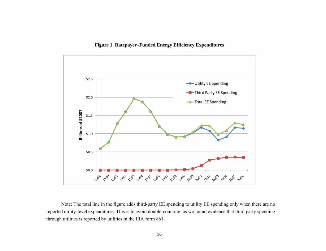
36

Figure 1. Ratepayer–Funded Energy Efficiency Expenditures

Note: The total line in the figure adds third-party EE spending to utility EE spending only when there are no

reported utility-level expenditures. This is to avoid double-counting, as we found evidence that third party spending

through utilities is reported by utilities in the EIA form 861.

$0.0

$0.5

$1.0

$1.5

$2.0

$2.5Billion

s of $2007

Utility EE Spending

Third Party EE Spending

Total EE Spending

37

Figure 2. Stringency of Building Codes in 2007

38

Figure 3: Long-term Effect of DSM Spending from the Baseline Model

Notes: the top graph is based on results from NLS (model 1 in table 2) and the bottom graph is

based on results from GMM (model 3 in table 2).

0 2 4 6 8 10 12 14 16 18 20-0.05

0

0.05

0.1

0.15

0.2

95% Lower Bound

Time Path

Alternative Path

95% Upper Bound

0 2 4 6 8 10 12 14 16 18 20-0.05

0

0.05

0.1

0.15

0.2

95% Lower Bound

Time Path

Alternative Path

95% Upper Bound

Year

Year

39

Figure 4: Long-term Effect of DSM Spending using Weibull Distribution

Notes: the top graph is based on results from NLS (robustness 4 in table 5) and the bottom graph

is based on results from GMM (robustness 4 in table 5).

0 2 4 6 8 10 12 14 16 18 20-0.05

0

0.05

0.1

0.15

0.2

95% Lower Bound

Time Path

Alternative Path

95% Upper Bound

0 2 4 6 8 10 12 14 16 18 20-0.1

-0.05

0

0.05

0.1

0.15

0.2

0.25

95% Lower Bound

Time Path

Alternative Path

95% Upper Bound

Year

Year

40

References

ACEEE (American Council for an Energy Efficient Economy) (2004). “Summary Table of

Public Benefit Programs and Electricity Restructuring.” Accessed at

http://www.aceee.org/briefs/apr04_01.htm (July 6, 2009).

Aroonruengsawat, Anin, Maximilian Auffhammer and Alan Sanstad (2009). “The Impact of

State-Level Building Codes on Residential Electricity Consumption.” Working paper.

Auffhammer, Maximilian, Carl Blumstein, and Meredith Fowlie ( 2008). “Demand Side

Management and Energy Efficiency Revisited.” The Energy Journal 29(3): 91–104.

Brennan, Timothy (1998). “Demand-Side Management Programs under Retail Electricity

Competition.” Resources for the future discussion paper 99-02.

California Energy Commission ( 2007). California Energy Demand 2008 - 2018, Staff Revised

Forecast, CEC-200-2007-015-SF2, November.

Chamberlain, G. (1987). “Asymptotic Efficiency in Estimation with Conditional Moment

Restrictions,” Journal of Econometrics 34: 305-334.

Costa, Dora and Matthew Kahn (2009). “Toward a Greener California: An Analysis of

Household Variation in Residential Electricity Purchases”, mimeo, November.

Damodaran, Aswath ( 2006). Damodaran on Valuation: Security Analysis for Investment and

Corporate Finance, 2nd edition, Wiley and Sons Inc.

Efficiency Vermont (2008). Efficiency Vermont Annual Report, Accessed at

http://www.efficiencyvermont.com/stella/filelib/2008_Efficiency_Vermont_Annual_Rep

ort.pdf, (November 11, 2009)

EIA (U.S. Energy Information Administration) (2009). Annual Energy Review 2008. DOE/EIA-

0384(2008). Washington, DC: EIA.

Eto, J., E. Vine, L. Shown, R. Sonnenblick, and C. Paine (1996). “The Total Cost and Measured

Performance of Utility-Sponsored Energy Efficiency Programs,” The Energy Journal 17

(1): 31-51.

Eto, Joseph, Chuck Goldman, and Steve Nadel (1998). “Ratepayer-Funded Energy-Efficiency

Programs in a Restructured Electricity Industry: Issues and Options for Regulators and

Legislators,” LBNL-41479, May.

41

Eto J., S. Kito, L. Shown, and R. Sonnenblick (2000). “Where Did the Money Go? The Cost and

Performance of the Largest Commercial Sector DSM Programs.” The Energy Journal

21(2):23-49.

Freidrich, Katherine, Maggie Eldridge, Dan York, Patti Witte, and Marty Kushler (2009). Saving

Energy Cost-Effectively: A National Review of the Cost of Energy Saved through Utility-

Sector Energy Efficiency Programs. ACEEE Report Number U092, September.

Washington, DC: ACEEE.

Fickett A.P., Clark W. Gellings, and Amory B. Lovins (1990). “Efficient Use of Electricity.”

Scientific American 263 (September): 64–74.

Gillingham, Kenneth, Richard G. Newell, and Karen Palmer (2004). “Retrospective Examination

of Demand Side Energy Efficiency Policies.” Resources for the Future Discussion Paper

04-19 REV (June).

Gillingham, Kenneth, Richard G. Newell, and Karen Palmer (2006). “Retrospective Review of

Energy Efficiency Policies.” Annual Review of Environment and Resources 31: 161–192.

Gillingham, Kenneth, Richard G. Newell, and Karen Palmer (2009). “Energy Efficiency

Economics and Policy.” Annual Review of Resource Economics 1:14.1–14.23.

Granade, Hanah Choi, Jon Creyts, Anton Derkach, Philip Farese, Scott Nyquist, and Ken

Ostroski (2009). Unlocking Energy Efficiency in the U.S. Economy. McKinsey Global

Energy and Materials, July. McKinsey and Company.

Horowitz, Marvin J. (2004). “Electricity Intensity in the Commercial Sector: Market and Public

Program Effects.” The Energy Journal 25(2): 115 – 137.

Horowitz, Marvin J. (2007). “Changes in Electricity Demand in the United States from the 1970s

to 2003.” The Energy Journal 28(3):93–119.

Horowitz, Marvin J. (2010). “EIA’s Energy Efficiency Program Data: Toxic if Swallowed,”

paper presented at the 15th Annual POWER conference, Energy Institute at Haas,

University of California, Berkeley, California, March 18.

Jacobsen, Grant D. and Matthew J. Kotchen (2010). “Are Building Codes Effective at Saving

Energy? Evidence from Residential Billing Data in Florida,” NBER Working Paper

16194 (June).

Jaffe, Adam B., and Robert N. Stavins (1995). “Dynamic Incentives of Environmental

Regulations: The Effects of Alternative Policy Instruments on Technology Diffusion,”

Journal of Environmental Economics and Management 29(3): 43–63.

42

Joskow, Paul and Donald Marron (1992). “What Does a Negawatt Really Cost? Evidence from

Utility Conservation Programs." The Energy Journal 13: 41–74.

Khawaja, Sami, Patricia Koss, and Brian Hedman (2001). “System Benefits Charge: Economic

Impacts and Implications.” The Electricity Journal 14(5):25–32.

Loughran, David S., and Jonathan Kulick (2004). “Demand-Side Management and Energy

Efficiency in the United States.” The Energy Journal 25(1): 19–41.

Nadel Steven (1992). “Utility Demand-Side Management Experience and Potential: A Critical

Review.” Annual Review of Energy and the Environment 17:507–535.

Nadel, Steven, and Howard Geller (1996). “Utility DSM: What Have We Learned? Where Are

We Going?” Energy Policy 24(4): 289–302.

Nadel, Steven, and Marty Kushler (2000). “Public Benefit Funds: A Key Strategy for Advancing

Energy Efficiency.” The Electricity Journal 13(8):74–84.

National Academy of Sciences (2009). Electricity from Renewable Resources: Status, Prospects

and Impediments. America’s Energy Future Panel on Electricity from Renewable

Resources. Washington, DC: National Academies Press.

Newey, Whitney, and Daniel McFadden (1986). “Large Sample Estimation and Hypothesis

Testing.”, in: R. F. Engle and D. McFadden (ed.), Handbook of Econometrics, 1(4):

2111-2245. Elsevier.

Pacific Gas and Electric (2010). Energy Efficiency Program Portfolio Annual Report for 2009,

report to California Public Utility Commission, June.

Parformack, Paul W., and Lester B. Lave (1996). “How Many Kilowatts Are in a Negawatt?

Verifying ‘Ex Post’ Estimates of Utility Conservation Impacts at the Regional Level.”

The Energy Journal 17(4): 59–88.

PJM Independent System Operator (2006). Executive Report. Accessed at

http://www.pjm.com/~/media/committees-groups/committees/mc/20070125-item-03a-

december-2006-executive-report-markets.ashx, October 29, 2009.

Reid, Michael (2009). “Using U.S. Energy Information Administration Data to Benchmark

Electric Utility DSM Portfolios,” paper prepared for the 2009 International Energy

Efficiency Program Evaluation Conference, Portland, Oregon, June.

RGGI (Regional Greenhouse Gas Initiative) Emissions Leakage Multi-State Staff Working

Group (2008). Potential Emission Leakage and the Regional Greenhouse Gas Initiative.

43

Final Report, March. Accessed at http://www.rggi.org/docs/20080331leakage.pdf, April

3, 2008.

RGGI, Inc. (2011). “Investment of Proceeds from RGGI CO2 Allowances,” February.

Accessed at http://www.rggi.org/docs/Investment_of_RGGI_Allowance_Proceeds.pdf,

March 8, 2011.

Takahashi, Kenji and David A. Nichols (2008). “The Sustainability and Costs of Increasing

Efficiency Impacts: Evidence from Experience to Date”, presentation at the 2008 ACEEE

Summer Conference, August. Accessed at http://www.synapse-energy.com/cgi-

bin/synapsePublications.pl?filter_type=Year&filter_option=2008&advanced=false,

November 11, 2009

U.S. EIA (Energy Information Administration) (2008). Annual Energy Review 2008. DOE/EIA

– 0384(2008), June.

York, Dan and Marty Kushler (2005). ACEEE’s 3rd National Scorecard on Utility Public

Benefits Energy Efficiency Programs: A National Review and Update of State-Level

Activity. U054, Washington, DC: American Council for an Energy-Efficient Economy.

44

Appendix

 

 

Table A-1. Third-Party DSM Expenditures: State, Year, and Data Source (millions of 2007$)

State 1998 1999 2000 2001 2002 2003 2004 2005 2006 Administrator

Illinois 0.00 0.00 0.00 0.00 0.00 3.21 3.12 0.93 1.06

Department of Commerce and Economic Opportunity(Energy Efficiency Trust Fund)

Maine 0.00 0.00 0.00 0.00 0.00 2.80 5.11 8.26 9.33 Efficiency Maine

Michigan 0.00 0.00 0.00 0.00 1.12 2.51 3.66 3.70 2.89

Michigan Public Service Commission (The Low-Income and Energy Efficiency Fund)

New Jersey 0.00 0.00 0.00 66.19 107.25 99.44 101.52 90.53 81.78

New Jersey Board of Public Utilities (New Jersey Clean Energy Collaborative)

New York 7.86 12.05 30.54 80.34 137.77 160.32 152.87 150.86 155.01

New York State Energy Research and Development Authority

Oregon 0.00 0.00 0.00 0.00 8.41 27.46 43.89 54.49 46.69 Energy Trust of Oregon

Vermont 0.00 0.00 6.71 10.30 12.63 14.59 15.31 16.01 15.24 Efficiency Vermont

Wisconsin 0.00 0.00 0.00 0.00 29.07 50.65 42.62 41.48 40.84 Focus on Energy

Total 7.86 12.05 37.25 156.83 296.24 360.98 368.11 366.26 352.84