Cost effective environmental control technology for utilities

Advances in Environmental Research 8(2003) 173–196

1093-0191/03/$ - see front matter� 2002 Elsevier Science Ltd. All rights reserved.doi:10.1016/S1093-0191(02)00129-6

Cost effective environmental control technology for utilities

Yan Fu , Urmila M. Diwekar *a b,

Ford Research Laboratory, Ford Motor Company, Dearborn, MI 48187, USAa

Civil and Environmental Engineering Department, Carnegie Mellon University, Pittsburgh, PA 15213, USAb

Abstract

On September 24, 1998, new regulations announced by the US EPA require 22 eastern states plus the District ofColumbia to develop state implementation plans to reduce ground-level ozone through the reduction of nitrogen oxide(NOx) emissions(Cooper, 1998). This plan calls for a 28% NOx cut in the summer time(1.2 million tons) by 2007.This calls for utilities to develop new, efficient, and robust post-combustion NOx control technologies. A newenvironmental control technology called low temperature oxidation(LTO) system, which can reduce NOx emissionsbelow measurable levels(i.e. 2 ppm using process analyzers) at low temperature(125–3258F), was awarded thebest available control technology and the lowest available emission reduction technology by the US EPA in April1998. Ozone is employed to oxidize nitric oxide(NO) to dinitrogen pentoxide(N O ) at a low temperature in an2 5

oxidizer, which is then easily absorbed by water in a scrubber. Bench scale and pilot plant tests have shown that theLTO process can almost completely remove the NOx emissions(i.e. NOx emissions are below levels measurableusing process analyzers). This proved that the LTO system is an attractive process to meet the stricter NOx regulations.There are multiple benefits of the LTO system besides removal of NOx emissions, includes reduction of SOx andCO emissions, and no secondary air emissions(NH , N O). In order to obtain minimum NOx emissions, extra ozone3 2

needs to be supplied. The cost of the process also increases nonlinearly as emissions decrease. This poses achallenging multiobjective optimization problem where emissions like NOx and SOx need to be minimized, whileminimizing the system cost as well as extra ozone. This problem is addressed using a new and efficient multiobjectiveoptimization framework. This framework will provide designs that are cost effective as well as environmentallyfriendly.� 2002 Elsevier Science Ltd. All rights reserved.

Keywords: Nonlinear multiobjective optimization; MINSOOP algorithm; Hammersley sequence sampling; NOx control; NOxabsorption

1. Introduction

Nitrogen oxides(NOx) play a major role, togetherwith volatile organic compounds in the atmosphericreactions that produce ozone and acid rain, and mayaffect both terrestrial and aquatic ecosystems. NOx isformed when fuel is burned at high temperatures. Thetwo major emissions sources are transportation andstationary fuel combustion sources such as electric

*Corresponding author. Tel.:q1-412-268-3003; fax:q1-412-268-7813.

E-mail address: [email protected](U.M. Diwekar).

utilities and industrial boilers. The EPA uses NOx asone of the ‘criteria pollutants’ to indicate air quality.As environmental regulations become more and more

stringent, many industries will have to carefully considerthe long-term high level of NOx emissions reductionfrom their boilers, furnaces, gas turbines, chemicalreactors, incinerators, diesel engines, kilns and thermaloxidizers. Cannon Technology Inc., in collaboration withBOC Gases has developed the low temperature oxida-tion (LTO) process for removing NOx emissions. Fig.1 shows the LTO process diagram for a small-scaleindustrial boiler application. In Fig. 1, the exhaust fluegas from the boiler is cooled in a high temperatureeconomizer, giving up heat to preheat the boiler feed

174 Y. Fu, U.M. Diwekar / Advances in Environmental Research 8 (2003) 173–196

Fig. 1. The LTO process diagram for a small-scale industrial boiler application.

water. The gas is then cooled to its dew-point tempera-ture in a condenser and a portion of the water vapor inthe gas is condensed. Ozone is injected into the gas asit leaves the condenser and is thoroughly mixed withthe gas in a static mixer. The NOx in the gas is oxidizedin the oxidation chamber to dinitrogen pentoxide(N O ), with part of CO oxidized to CO and SO2 5 2 2

oxidized to SO . The pentoxide forms nitric acid vapor3

as it contacts the water vapor in the gas, and similarly,sulfite acid, sulfate acid, bicarbonate, and carbonate acidvapors are formed. Then nitric acid vapor is absorbedin the scrubber as dilute nitric acid and is then neutral-ized by the dilute sodium carbonate in the scrubberforming sodium nitrate. Accordingly, sodium bicarbon-ate, sodium carbonate, sodium sulfite, sodium sulfateare produced. These dilute salts can be disposed to thesanitary sewer system for small-scale industrial boilers.For large-scale systems, by-product recovery can be anoption. There are multiple benefits of the LTO systembesides the removal of NOx emissions, such as areduction in SOx, CO emissions, and other pollutants.In order to obtain minimum NOx emissions, extra ozoneneeds to be supplied. Also the cost of the processincreases nonlinearly as emissions decrease. This posesa challenging multiobjective optimization problemwhere emissions like NOx and SOx need to be mini-mized, while minimizing the system cost as well aslimiting extra ozone.In our previous works, a detailed model of the LTO

process based on a nonequilibrium modeling techniquewas developed and two major bottlenecks involved inmodeling this system such as numerical difficulties andtwo-point boundary value problem were solved as well(Fu et al., 1999, 2000). The cost model(Suchak andMay, 2000) of the LTO process is presented in Appendix

A of this paper. It should be noted here that we areusing the older LTO technology for this analysis. Thenew technology removes SOx and CO emissions moreefficiently than the results showed in this paper. Themultiobjective case study presented in the present paperdoes not include the ozone destruction part of thescrubber in the detailed model; the ozone slip is assumedto be less than 5 ppm in the current study. In the future,the model will include the ozone destruction reactions,and minimizing ozone slip would be included as anadditional objective with ozone destruction scrubberparameters as additional decision variables.The paper is divided into four sections. Section 2

describes the multiobjective optimization framework forthe LTO process. Section 3 presents the detailed casestudy with results. The final section highlights the majorconclusions.

2. Multiobjective optimization framework for theLTO process

The LTO non-equilibrium model(Fu et al., 2000)was augmented with the cost model of the process toformulate a complete LTO model(Fu, 2000). The modelis very complex consisting of 65 stiff differential equa-tions and 39 algebraic highly nonlinear equations andtakes approximately 2 min of CPU time to run on aDell PC with 400-MHz Pentium II Processor. Thiscomplete LTO model will be incorporated in a multiob-jective problem to obtain minimum cost and minimumemissions designs in this paper. In order to solve themultiobjective problem for obtaining minimum cost andminimum emission designs, a new efficient multiobjec-tive nonlinear programming algorithm called minimiza-tion of single objective optimization problems

175Y. Fu, U.M. Diwekar / Advances in Environmental Research 8 (2003) 173–196

(MINSOOP) is developed. This section briefly describesthe algorithm and how to formulate a multiobjectiveoptimization problem for the design of the LTO process.The following equations show a generalized multiob-

jective optimization problem

Minimize√B E

C F

D Gf x , is1,«,k, k02 (1)i

Subject to√B E

C F

D Gh x s0, I00I

√B EC F

D Gg x (0, J00J

l(x(u , js1,«,n,j j jr

xs x ,«,xŽ .1 n

The problem under consideration involves a set ofn

decision variables represented by the vector√

(x)s

The equality constraints√

(x ,x ,«,x ). h (x),I01 2 n I

and inequality constraints√

n0: R ™R, g (x),J0J

are real-valued(possibly nonlinear) con-n0: R ™Rstraint functions andl andu are given lower and upperj j

bounds of decision variablex . Without loss of gener-j

ality, we assume that all the objective functions are tobe minimized simultaneously(Note that an objective ofthe maximization type could be converted to one of theminimization type by multiplying the objective functionby y1).The solution of a multiobjective optimization is a set

of solution alternatives called the Pareto set. For eachof these solution alternatives, it is impossible to improveone objective without sacrificing the value of anotherobjective relative to some other solution alternatives inthe set. There is a large array of analytical techniquesfor multiobjective optimization problems. One of thewidely used methods for nonlinear problems is theconstraint method(Haimes et al., 1971; Cohon, 1978;Zeleny, 1982). The basic strategy is to transform themultiobjective optimization problem into a series ofsingle objective optimization problems. The idea is topick one of the objectives to minimize(say Z ) whilel

each of the others(Z , is1,«, k, i/l) is turned into ani

inequality constraint with parametric right-hand sides(´ , is1,«, k, i/l). The problem takes the formi

MinimizerB E

C F

D GZsf x (2)l l

Subject torB E

C F

D GZsf x (´ , is1,«,k, i/li i i

rB EC F

D Gh x s0, I00I

rB EC F

D Gg x (0, J00J

l(x(u , js1,«,nj j j

rB EC F

D Gx s x ,«,xŽ .1 n

Solving repeatedly for different values of´ ,«, ´ ,i ly1

´ ,«, ´ leads to the Pareto set. This method needslq1 k

to obtain solutions for a large number of single objectiveoptimization problems. One straightforward approach isto place the points along equally spaced intervals on a(ky1)-dimensional grid, which represents the tradition-al constraint method. Although this is a good arrange-ment, the number of points required increases rapidlyas the number of objectives increases. For example, ifthere are six objectives and five of them are evaluatedover 10 points for each objective, we would have tosolve 100 000 optimization problems. Alternatively onecan use a Monte Carlo sampling(MCS) technique,where the points are chosen randomly. The remarkablefeature is that the MCS methods are unlikely to scaleexponentially with increasing objective functions. How-ever, MCS methods are based on pseudo-random num-ber generators, and do not have good uniformity. TheLatin hypercube sampling(LHS, Iman and Shortencar-ier, 1984) technique is one form of stratified samplingthat can reduce the variance in the Monte Carlo estimateof the integrand. The range of each inputZ is dividedi

into nonoverlapping intervals of equal probability. Onevalue from each interval is selected at random withrespect to the probability density in the interval. Thenvalues that were obtained forZ are paired in a random1

manner (i.e. equally likely combinations) with the nvalues of Z and thesen pairs are combined withn2

values ofZ and so on to formn (ky1)-tuplets. The3

random pairing is based on a pseudo-random numbergenerator. The main drawback of this stratificationscheme is that it is uniform in one dimension and doesnot provide uniformity properties in(ky1)-dimensions.Recently, Kalagnanam and Diwekar(1997) developedan efficient sampling technique called the Hammersleysequence sampling(HSS) technique based on a quasi-random number generator. It uses the Hammersleypoints to uniformly sample a(ky1)-dimensional hyper-cube, and the results revealed that the Hammersleypoints provide the optimal location for the sample pointsso as to obtain better uniformity in the(ky1)-dimen-sion. It was found that the HSS technique is at least 3–100 times faster than LHS and Monte Carlo techniques(Kalagnanam and Diwekar, 1997).


Fig. 2. Multiobjective optimization framework for the LTO process.

The new multiobjective optimization algorithm MIN-SOOP uses the HSS technique to generate combinationsof the right-hand sides , (is1,«, k, i/l) of thei

traditional constraint method. For details of this algo-rithm, please refer to Fu and Diwekar(2003). The stepsfor a multiobjective problem withk objectives(to beminimized) are listed as follows:

Step 1. Solvek single objective optimization problemsindividually with the original constraints of a multiob-jective problem to find the optimal solution for each ofthe individualk objectives.

Step 2. Compute the value of each of thek objectivesat each of thek individual optimal solutions. In thisway, an approximation of the potential range of valuesfor each of thek objectives is determined. These valuesconstitute the payoff table. The minimum possible valueis the individual optimal(minimizing) solution. Theapproximate maximum possible value of the Pareto setis the maximum value for that objective found whenminimizing the otherky1 objectives individually.

Step 3. Select a single objective(e.g. Z ) to bel

minimized. Transform the remainingky1 objectivesinto inequality constraints of the formZ (´ , is1,«,i i

k, i/l and add these newky1 constraints to the originalset of constraints. Then the original multiobjectiveoptimization problem is transformed into a family ofsingle objective optimization problems with parametricright-hand sides.

Step 4. Select a desired number of single objectiveoptimization problems to be solved to represent thePareto set. Using the HSS technique to generate thedesired number of combinations of the inequality con-

straint values ,«, ´ , ´ ,«, ´ within the rangei ly1 lq1 k

determined inStep 2.Step 5. Solve the constrained problems set up in step

4 for every combination of the right-hand-side valuesdetermined in step 3. These feasible solutions form anapproximation for the Pareto set.Fig. 2 shows the strategy of the multiobjective optimal

design of the LTO process. In our earlier work(Fu etal., 1999) to avoid the two-point boundary value prob-lem in modeling, we had to use an optimization frame-work so as to minimize the error in predictingconcentrations of input liquid accurately. It can be seenfrom Fig. 2 that the objectives are minimizing the cost,NOx and SOx emissions, while the error in predictingconcentrations of input liquid in the scrubber is aconstraint in this framework. This allows one to simul-taneously solve the modeling and optimization problem.In practice in order to obtain minimum NOx emissions,extra ozone is added to the system, which not onlyincreases the system cost but also causes ozone slip.Therefore, a feedback system is installed at the top ofthe scrubber of the LTO process. When the NOxemissions are high, the feedback system can control theozone generator to provide more ozone. When the ozoneconcentrations are high, the feedback system can informthe ozone generator to reduce ozone generation. In thisway, ozone slip can be minimized. The drawbacks are(1) the sensor of the feedback system is quite expensiveand requires high maintenance cost and(2) the systemis actually operated dynamically instead of in steadystate. Here our optimization approach to solve thisproblem is to add another constraint to make sure that


Table 1The bounds and the base design values of the key decision variables for the multiobjective optimization case study of the LTOprocess

Symbols Name of key decision variable Unit Lower Upper Basexj xj bounds bounds design

xLj xUj xoj

x1 Diameter of the oxidizer m 0.5 1.5 0.8x2 Length of the oxidizer m 2.0 25.0 24.4x3 Mole ratio of O yNox3 Moleymole 1.0 2.0 1.6x4 Diameter of the scrubber m 0.5 1.5 0.9x5 Height of the scrubber m 1.0 2.5 1.5x6 Liquid flow rate of the scrubber galymin 50 150 85x7 Liquid output concentrations of NaHCOa3 Moleymole of H O2 1.0Ey6 1.0Ey2 b

x8 Liquid output concentrations of Na COa2 3 Moleymole of H O2 1.0Ey6 1.0Ey2 b

x9 Liquid output concentrations of Na SOa2 4 Moleymole of H O2 1.0Ey6 1.0Ey2 b

x10 Liquid output concentrations of Na SOa2 3 Moleymole of H O2 1.0Ey6 1.0Ey2 b

x11 Liquid output concentrations of NaNOa2 Moleymole of H O2 1.0Ey6 1.0Ey2 b

x12 Liquid output concentrations of NaNOa3 Moleymole of H O2 1.0Ey6 1.0Ey2 b

x13 Liquid output concentrations of Oa3 Moleymole of H O2 1.0Ey6 1.0Ey2 b

Intermediate variables that are used by the optimizer to keep the error in predicting the input liquid concentrations in the scrubbera

(due to the two-point boundary value problem) less than or equal to 10 to ensure the model’s accuracy.y6

Values for these intermediate variables are automatically calculated by the optimizer with minimizing the error in predicting theb

input liquid concentrations in the scrubber as the objective.

the ozone slip is less than or equal to the allowablelimit (which can be easily changed according to custom-er’s request). By solving a minimal number of singleobjective optimization problems using the efficientMINSOOP algorithm (Fu and Diwekar, 2003), a set ofPareto optimal designs for the LTO process will beobtained. Then the approximate Pareto surface for themultiobjective problem will be drawn. This will behelpful for understanding the characteristics of the LTOprocess and for designing the system to be cost efficientwhile keeping all kinds of pollutant emissions at verylow levels.

3. Case study

In this section, we will demonstrate how an efficientmultiobjective optimization framework can be a valua-ble tool for designing the LTO process, so that it notonly can reduce NOx and SOx emissions to the lowestlevels, but also can minimize the system cost. At thesame time, the constraints setup for the optimizationproblem can ensure the model’s accuracy as well aslimiting extra ozone in the steady-state operatingcondition.

3.1. Formulating the multiobjective optimizationproblem

In this case study, we would like to provide optimaldesign alternatives for the LTO process in order toreduce pollutant emissions of a 400-HP boiler operatedat a 60% load condition(Suchak and May, 2000) with

a 10 713 lbyh of flue gas, with 39 ppm NOx, 500 ppmSOx, and 10 ppm CO at the temperature of 788F andpressure of 1 atm. The capital cost for the system isspread over a 10-year-period. The multiobjective optim-ization formulation for this case study is described inEq. (3).

Minimize NOx emissionsSOx emissionsCost

(3)

Subject to Error in predicting concentrations of inputy6liquid of the scrubber(10

O emission(5 ppmDifferential3

algebraic equations: Reactions, massbalance and energy balancex (x(x ,js1y13Lj j Uj

Here the NOx and SOx emissions and cost areminimized concurrently. At the same time, the error inpredicting concentrations of input liquid of the scrubberis less than or equal to 10 so as to ensure the model’sy6

accuracy and ozone emission is less than or equal to 5ppm to guarantee low ozone slip. Here we choose 13key decision variables, which are identified to be impor-tant to the LTO process’s performance, cost, and mod-el’s accuracy according to the engineering knowledgeand previous modeling experience. The details of thesedecision variables are defined in Table 1. It can be seen


from Table 1 that only six variables(x ,«, x ) out of1 6

the 13 decision variables are the real decision variables.The rest of them are intermediate variables used by theoptimizer to ensure the model’s accuracy due to thetwo-point value problem in the scrubber (Fu, 2000).The ranges and the base design values for these decisionvariables are determined by the heuristic experience.It is worthy of mention that two important operating

variables, pressure and temperature, are not listed askey decision variables in this case study. Even thoughhigher pressure can help to remove the pollutant emis-sions, according to model simulations, it demands addi-tional constraints to the structural materials and is hardto control. Therefore, we intend to keep the LTO processoperating at an open pressure(1-atm) condition. Thereasons that temperature is not included in the keydecision variables are as follows:(1) It is well knownby engineering knowledge and simulation experiencethat a relatively higher temperature often has positiveimpacts on the LTO performance. If it is defined as adecision variable, the optimizer always tends to chooseits upper bound.(2) In real practice, temperature isusually predefined by specified application. In general,the LTO process can reduce NOx emissions belowdetection limits(2 ppm) at low temperature in the rangeof 125–325 8F. At a temperature exceeding 3258F,ozone decomposes rapidly and the cost will increasedramatically without benefiting the pollutant emissionsreduction.(3) At a higher temperature()170 8F), thecurrent model parameters need to be tuned with exper-imental data to adjust the temperature impacts on dif-ferent chemical reaction and absorption rate coefficients.Therefore, here we choose to operate the LTO processat a specified very low temperature(78 8F), which is arelatively bad operating condition for the LTO process.In this way, we can observe a relatively wide range ofNOx and SOx removal rates, see the effects to thesystem cost, and evaluate the applicability of the newand efficient multiobjective optimization(MINSOOP)algorithm in solving a large-scale problem in its worst-case condition.The LTO process will have better performances at

higher temperatures(-325 8F). Table 2 shows thedifferent performance of the base design at two differenttemperature conditions: the current temperature for thecase study(78 8F) and a slightly higher temperature(125 8F). Results show that at the higher temperature(125 8F), the base design of the LTO process cansignificantly reduce NOx and SOx emissions with muchless ozone slip and only slightly higher cost than at thecurrent case study temperature(78 8F). The reason forthis is that chemical reaction and absorption ratesincrease significantly when the temperature increasesfrom 78 to 1258F. This helps to reduce NOx and SOx

emissions, and also reduces extra ozone. Even though,in this case study, the aim is to use the efficientMINSOOP algorithm(Fu and Diwekar, 2003) to findthe optimal design alternatives at its worst condition(78 8F), the LTO process performances and costs at thecurrent temperature(78 8F) and those at the slightlyhigher temperature(125 8F) for the same designs willbe compared at the end of this section.

3.2. Generating the payoff table

The nonlinear optimizer is employed to solve threesingle objective optimization problems separately, keep-ing the error in predicting concentrations of input liquidof the scrubber less than or equal to 10 and ozoney6

emissions less than or equal to 5 ppm for each of thethree objectives. The optimizer is started from 50different randomly generated initial points and the min-imum value is retained as the optimal solution due tothe nonlinear nonconvex nature of the problem. Thenthe values of the other two objectives are calculated ateach of the three optimal solutions. These objectivevalues are listed in the payoff table shown in Table 3.In this way, an approximation of the potential rangesfor all three objectives in the Pareto set is determined.The minimum possible value is the individual optimal(minimizing) solution. The approximate maximum pos-sible value of the Pareto set is the maximum value forthat objective found when minimizing the other twoobjectives individually. In this case study, the concentra-tion of NOx emissions is between 5 and 36 ppm, theconcentration of SOx emissions ranges from 73 to 295ppm and the cost is within 13.77–16.65 $yh.Table 4 lists the details of the decision variables,

objectives, and constraints for the base design and theabove three single objective optimal designs. From Table4, we can see that the oxidizer does not reduce SOxemissions because the concentration of SOx emissionsat the exit of the oxidizer(500 ppm) is the same as theinput concentration of SOx emissions for all fourdesigns, but it removes most of the NOx emissionsexcept the design(D). Most of the SOx emissions andpart of the NOx emissions are reduced in the scrubber.Even the worst one(D) can reduce SOx emissionsmore than 200 ppm(at 40% SOx emissions removalrate). This certainly implies that the LTO process notonly can reduce NOx emissions to very low level, butis also an attractive process to reduce the SOx emissions.The total cost of the LTO process for this case study

comes mainly from the total fixed cost, in which thecosts for a blower, analyzers, control hardware, valves,and labor are relatively the same for all four designs,which means they are not affected significantly by thedecision variables identified in this case study. The totaloperating cost is a relatively smaller part of the total


Table 2Compare the performances of the base design for the case study of the LTO process at two different temperature conditions

Current temperature(78 8F) High temperature(125 8F)

ppm % removal ppm % removalrate rate

NOx emissionsOxidizer exit 23 40.34 16 60.22Scrubber exit 20 47.75 4 88.74SOx emissionsOxidizer exit 500 0.00 500 0.00Scrubber exit 191 61.80 42 91.56

Cost Cost($yh) % in total cost Cost($yh) % in total cost

Oxidizer cost 0.27 1.84 0.27 1.84Ozone manifold cost 0.21 1.42 0.21 1.41Ozone generator cost 0.88 5.88 0.88 5.87Blower cost 0.37 2.49 0.39 2.60Chiller cost 0.04 0.28 0.04 0.27Analyzers cost 3.96 26.61 3.96 26.56Control hardware, valves, etc., cost 1.34 9.00 1.34 9.00Scrubber cost 0.41 2.76 0.41 2.75

Fixed capital cost 7.49 50.28 7.51 50.33Maintenance cost 1.18 7.91 1.18 7.92Insurance cost 0.50 3.38 0.50 3.38Labor cost 3.95 26.48 3.95 26.44

Total fixed cost 13.12 88.04 13.14 88.06Total operating cost 1.78 11.96 1.78 11.94Total cost 14.90 100.00 14.92 100.00

Extra ozone ppm % in total input ozone ppm % in total input ozone

Oxidizer exit 13 21.19 9 14.27Scrubber exit 9 14.20 2 3.39

Error in predicting concentrations 4.30Ey07 4.20Ey07of input liquid of the scrubber

Notes: Fixed capital cost is the sum of costs for oxidizer, ozone manifold, ozone generator, blower, chiller, analyzers, controlhardware, valves, etc., and scrubber. Total fixed cost is the sum of costs for fixed capital, maintenance, insurance and labor. Totalcost is the sum of total fixed cost and total operating cost.

Table 3Payoff table for the case study of the LTO process

Objective Symbol NOx SOx Cost P aError Extra

i emissions emissions ($yh) ozone(ppm) (ppm) (ppm)

Min NOx emission 1 5 130 16.65 1.0Ey06 5Min SOx emission 2 9 73 15.64 1.0Ey06 5Min cost 3 36 295 13.77 4.5Ey7 2

Lower bound ZiL 5 73 13.77Upper bound ZiU 36 295 16.65

P means error in predicting concentrations of input liquid of the scrubber.aError


Table 4The details of the decision variables, objectives and constraints for the base design and the initial three single objective optimaldesigns

Base design Min NOx Min SOx Min costA emissions emissions D

B C

Decision variablesDiameter of the oxidizer(m) 0.8 1.5 1.5 0.5Length of the oxidizer(m) 24.4 25.0 22.1 4.3Mole ratio of O yNOx3 1.6 1.9 1.7 1.0Diameter of the scrubber(m) 0.9 1.5 0.5 0.5Height of the scrubber(m) 1.5 2.3 2.2 1.0Liquid flow rate of the scrubber(galymin) 85 150 150 74

NOx emissions (3) (1) (2) (4)Oxidizer exit(ppm) 23 10 10 38Scrubber exit(ppm) 20 5 9 36

SOx emissions (3) (2) (1) (4)Oxidizer exit(ppm) 500 500 500 500Scrubber exit(ppm) 191 130 73 295

Cost (2) (4) (3) (1)Oxidizer cost($yh) 0.27 0.86 0.82 0.04Ozone manifold cost($yh) 0.21 0.44 0.41 0.09Ozone generator cost($yh) 0.88 0.97 0.92 0.65Blower cost($yh) 0.37 0.37 0.37 0.37Chiller cost($yh) 0.04 0.05 0.04 0.03Analyzers cost($yh) 3.96 3.96 3.97 3.96Control hardware, valves, etc., cost($yh) 1.34 1.34 1.34 1.34Scrubber cost($yh) 0.41 0.90 0.20 0.17

Fixed capital cost($yh) 7.49 8.89 8.08 6.65Maintenance cost($yh) 1.18 1.40 1.27 1.05Insurance cost($yh) 0.50 0.60 0.54 0.45Labor cost($yh) 3.95 3.95 3.95 3.95

Total fixed cost($yh) 13.12 14.93 13.83 12.09Total operating cost($yh) 1.78 1.83 1.80 1.68Total cost($yh) 14.90 16.66 16.26 13.77

Error in predicting concentrations (6) (6) (6) (6)of input liquid of the scrubber

4.30Ey07 1.00Ey06 1.00Ey06 4.40Ey07

Extra ozone (=) (6) (6) (6)Oxidizer exit(ppm) 13 10 7 3Scrubber exit(ppm) 9 5 5 2

cost and it changes slightly for the four designs in thecurrent case study.The four designs are ranked according to the NOx

emissions, SOx emissions, and cost from the best toworst as(1)–(4) shown in Table 4. The NOx emissionsincrease from the case of minimizing NOx emissions(B), to that of minimizing SOx emissions(C), to thebase design(A), and to that of minimizing cost(D) insequence. According to the SOx emissions, the designsare ranked from the best to the worst as C, B, A andD. The total cost increases from D, to A, to C and toB in order. For all four designs, the error in predicting

concentrations of input liquid of the scrubber is lessthan or equal to 10 , which means that this constrainty6

is satisfied by all of them. However, for the constraintthat extra ozone is less than or equal to 5 ppm, onlythe three single objective optimal designs(B, C and D)are feasible designs. For the base design the extra ozoneis 9 ppm, higher than the 5 ppm limit in this case study,which means that the base design is not feasible in thissense. In summary, it is obvious that even with onlyfour designs, the decision-maker will choose a totallydifferent design if he or she uses only one criterionfrom different points of view to make his or her


judgment. Therefore, it is necessary and important touse the efficient multiobjective optimization method tofind the insight information of the LTO process and toprovide the decision-maker with the design alternativesthat are not only minimizing the pollutant emissions butalso minimizing the cost at the same time.

3.3. Formulating a family of single objective optimiza-tion problems

Once the lower and upper bounds for each of thethree objectives are obtained, the original multiobjectiveoptimization problem is then transferred into a familyof single objective optimization problems in the generalform shown in Eq.(4).

Minimize CostSubject to NOx emissions(Rh NOxSOx emissions(Rh SOxError in predicting concentrations of input liquid of

y6the scrubber(10 O emission(5 ppm3

x (x(x , js1y13 (4)Lj j Uj

In this case study, cost is selected as the objective tobe minimized, NOx and SOx emissions are transferredinto inequality constraints with two parametric right-hand sides, Rh_NOx and Rh_SOx, and these two newconstraints are added to the original constraints of themultiobjective optimization problem. In this way, theoriginal multiobjective optimization problem is trans-formed into a family of single objective optimizationproblems. Here we choose to generate 100 additionalsingle objective optimization problems by efficientlyand uniformly changing the bounds of Rh_NOx andRh_SOx within their lower and upper bounds definedin Section 3.2(Rh_NOx within 5–35 ppm, Rh_SOxwithin 73–295 ppm) using the HSS technique. In thenext subsection the nonlinear optimizer will beemployed to find a set of minimum cost designs(opti-mal), which satisfy the corresponding limits for theNOx and SOx emissions specified in the currentsubsection.

3.4. Obtaining Pareto optimal solutions

Solving the appropriately formulated single objectiveoptimization problems for every combination of theright-hand-side values determined by the HSS techniqueusing the nonlinear optimizer, a set of Pareto optimaldesign alternatives are obtained. This includes 103(three initial single objective optimization problems plus100 additional transformed single objective optimizationproblems) Pareto optimal solutions. These Pareto opti-mal solutions form an approximation for the Pareto setof the LTO process for this case study. If a decision-

maker knows hisyher target, heyshe can search fromthese 103 optimal designs to find the final design thatis the most appropriate one to fit the decision-maker’simplicit value function. However, in most of the cases,the decision-maker would rather know the characteris-tics of the problem and the tradeoffs information amongobjectives before making his/her choice, which will beprovided in details in the next subsection.

3.5. Results and discussions

3.5.1. Payoff table for the case studyAs discussed in Section 3.2 the lower and upper

bounds of the Pareto set of this case study wereestimated from the three initial single objective optimaldesigns in the payoff table(Table 3). By comparing thedetails of decision variables, objectives and constraintsfor these optimal designs and the base design(Table4), valuable information about the reasons of causingthe significant differences among them can be obtained.Compared with the base design(A), the optimal

design for minimizing NOx emissions(B) has a largerdiameter and longer length oxidizer and higher moleratio of ozoneyNOx so that its costs for the oxidizer,ozone manifold, and ozone generator are higher whilereducing more NOx emissions. Design B also has alarger diameter and taller height of the scrubber and alarger liquid flow rate than the base design, whichcauses a higher scrubber cost but greater SOx emissionsremoval than Design A.Design C has the same diameter as Design B, but a

slightly shorter length of the oxidizer and a lower moleratio of ozoneyNOx than Design B. Therefore, itsoxidizer cost, ozone manifold and ozone generator costs,and its NOx emissions removal rate are lower thanDesign B, but they are still higher than the base design(A). In addition, Design C has a much smaller diameterand shorter height of the scrubber than Design B, whichgives a much lower scrubber cost than Design B.Because of the smaller diameter of the scrubber andlarger liquid flow rate, Design C can get the lowestSOx emissions of the four designs(A, B, C and D).Design D has the smallest diameters and shortest

lengths for the oxidizer and scrubber, the lowest moleratio of ozoneyNOx and the smallest liquid flow rateamong the four designs; therefore, it has the lowestcosts for every category except for the highest NOx andSOx emissions.The above results show that(1) the diameter and

length of the oxidizer are key variables that affect theNOx emissions and oxidizer cost,(2) the mole ratio ofozoneyNOx is an important variable that influences theNOx emissions and ozone generator costs, and(3) thediameter and length of the scrubber, and liquid flowrate are important variables for the SOx emissionsremoval and scrubber cost.


Fig. 3. Approximate 3D Pareto surface for the case study.

3.5.2. D surface plot for the approximate Pareto setOnce all the solutions for the appropriately formulated

single objective optimization problems are obtained, wecan use graphical means to draw the three-dimensional(3D) surface and contour plots for the approximatePareto surface. However, as only 103 designs areobtained, some approximations will be made for draw-ing the entire plot region.Fig. 3 shows the 3D surface plot for the approximate

Pareto set. This figure clearly shows that the multiob-jective optimization of the LTO process is a nonlinearnonconvex problem. Because the 3D Pareto surface isneither linear nor convex, many hills and valleys appearin the surface, which might provide chances for findinglower pollutant emissions and lower cost designs. Ingeneral when the concentration of SOx emissions is lessthan 200 ppm, the surface appears to be relatively linear.As the concentration of NOx emissions is reduced fromits upper bound(35 ppm) to its lower bound(5 ppm),the cost increases almost linearly with a very slighteffect caused by SOx reduction in this range.Table 5 shows the details of the decision variables,

objectives, and constraints for the three optimal designs(E, F and G) with SOx emissions approximately 80ppm and three other optimal designs(H, I and J) withSOx emissions approximately 135 ppm. From Table 5,we can see that, for designs E, F and G, the length ofthe oxidizer, the diameter and length of the scrubber,and the liquid flow rate are almost same; therefore theSOx emissions and the scrubber cost are approximatelythe same for these three designs. However, the diameterof the oxidizer and the mole ratio of ozoneyNOx

increase with the greater NOx emissions reduction,which also causes higher costs for the oxidizer, ozonemanifold, and ozone generator, and the total cost of theLTO system is increasing as well. The same phenomenacan also be seen through the details of H, I and Jdesigns in Table 5. However, for the lower SOx emis-sions designs(E, F, G), the length of the scrubber andliquid flow rate tend to be larger than those of higherSOx emissions designs(H, I, J), and the scrubber costsfor E, F and G are higher than those of H, I and J. Thiscauses the total cost of lower SOx emissions designs tobe higher than those of higher SOx emissions ones, butthe impact on the total cost by SOx emissions reductionis significantly lower than that from the NOx emissionsremoval.

3.5.3. Contour plot for the approximate Pareto setIn order to look into the details of the nonlinear part

of the Pareto surface, the contour plot of the approxi-mate Pareto surface is drawn in Fig. 4. Three majorthings catch our attention. First, designs within the smallcircle with a $15.1yh cost, approximately 25 ppm NOxemissions, and 250 ppm SOx emissions, can be domi-nated by a large number of designs located down andto the left, which have the same or less cost, lowerNOx andyor lower SOx emissions. Second, designs inthe circle with a $14.4yh cost at the top-right corner ofthe contour figure, can be conquered at least by designsin the same cost circle on its left, which have lowerNOx emissions and similar SOx emissions, and also bydesigns with the same cost but lower SOx emissions,and similar NOx emissions underneath. At this point,


Table 5The details of the decision variables, objectives, and constraints for the three optimal designs with SOx emissions approximately80 ppm and three other optimal designs with SOx emissions approximately 135 ppm

SOx emissions approximately 80(ppm)

SOx emissions approximately 135(ppm)

E F G H I J

Decision variablesDiameter of the oxidizer(m) 1.4 1.1 0.5 1.1 0.8 0.5Length of the oxidizer(m) 13.5 13.4 13.4 22.2 22.2 22.1Mole ratio of O yNOx3 1.5 1.4 1.1 1.5 1.3 1.2Diameter of the scrubber(m) 0.5 0.5 0.5 0.5 0.5 0.5Height of the scrubber(m) 2.0 2.0 2.1 1.5 1.5 1.5Liquid flow rate of the scrubber(galymin) 141 141 141 115 114 114

NOx emissionsOxidizer exit(ppm) 20 28 38 22 29 35Scrubber exit(ppm) 18 24 33 19 25 31

SOx emissionsOxidizer exit(ppm) 500 500 500 500 500 500Scrubber exit(ppm) 79 80 80 135 135 135

CostOxidizer cost($yh) 0.61 0.37 0.10 0.47 0.30 0.12Ozone manifold cost($yh) 0.30 0.22 0.09 0.28 0.22 0.15Ozone generator cost($yh) 0.85 0.80 0.69 0.83 0.78 0.75Blower cost($yh) 0.37 0.37 0.37 0.37 0.37 0.37Chiller cost($yh) 0.04 0.04 0.03 0.04 0.04 0.03Analyzers cost($yh) 3.96 3.96 3.96 3.96 3.96 3.96Control hardware, valves, etc., cost($yh) 1.34 1.34 1.34 1.34 1.34 1.34Scrubber cost($yh) 0.20 0.20 0.20 0.19 0.19 0.19

Fixed capital cost($yh) 7.66 7.29 6.78 7.48 7.19 6.91Maintenance cost($yh) 1.21 1.15 1.07 1.18 1.13 1.09Insurance cost($yh) 0.51 0.49 0.46 0.50 0.48 0.46Labor cost($yh) 3.95 3.95 3.95 3.95 3.95 3.95

Total fixed cost($yh) 13.32 12.87 12.25 13.11 12.75 12.40Total operating cost($yh) 1.77 1.74 1.70 1.76 1.74 1.72Total cost($yh) 15.08 14.62 13.95 14.86 14.49 14.12

Error in predicting concentrations 3.9Ey8 4.5Ey7 4.4Ey7 2.3Ey8 4.5Ey7 4.5Ey7of input liquid of the scrubber

Extra ozoneOxidizer exit(ppm) 7 7 3 7 7 7Scrubber exit(ppm) 5 5 2 5 5 5

we can say that, by using multiobjective optimizationapproach we can take some advantage of the nonlinearnon-convex feature of the problem to eliminate baddesigns. Furthermore, Fig. 4 also shows that the costtends to increase rapidly when the concentration of NOxemissions is low(-8 ppm) because the spacing of the$0.3yh cost contour lines, with respect to the NOxemissions, is much closer than in the higher NOxemissions region(08 ppm). Another important issuethat can be addressed by the multiobjective optimizationapproach is to provide explicit tradeoff informationamong different objectives and offer a reasonable num-

ber of attractive good designs for the decision-maker sothat heyshe can identify the final compromise designfor implementation, which is the focus of the followingdiscussions.

3.5.4. Normalized objectives plot for the base designand the approximate Pareto setLet’s first use the following equationwEq. (5)x to

normalize all three objectives within 0–1. The lowerthe normalized objective value is, the closer theZi

objectiveZ is to its lower bounds(Z ); and the higheri iL

the value is, the nearer the objectiveZ is to its upperZi i


Fig. 4. Contour plot of the approximate Pareto surface for the case study.

bounds(Z ). It is obvious that the smaller it is theiU

better the distribution for this case study.

ZyZŽ .i iLZs , is1,«,3 (5)i Z yZŽ .iU iL

Fig. 5 shows the different normalized objectives forthe base design(Design No. 0) and the 103 optimaldesigns that are sorted from the largest to the smallestas Design No. 1–103 by the NOx emissions. Fig. 5clearly shows that the trends of the NOx emissions andcost are conflicting, when the concentration of NOxemissions decreases the cost increases. As in Figs. 4and 5 also shows that the cost increases much morerapidly when the concentration of the NOx emissions isnear its lower bound. The trend of SOx emissions isdifferent from both the NOx emissions and the costbecause it jumps locally.Table 6 shows the details of the decision variables,

objectives, and constraints for three optimal designs(B,K and L) with NOx emissions lower than 8 ppm andthree other optimal designs(E, M and F) with NOxemissions higher than 8 ppm. Results show that for B,K, and L on average cost increases approximately$0.405yh to reduce the NOx emissions by 1 ppm, andfor E, M and F cost increases approximately $0.072yhto reduce 1 ppm more NOx emissions. It also can beseen that the average SOx emissions for designs of

lower NOx emissions are higher than that of higherNOx emissions. This means we need to pay more andsacrifice some of the SOx emissions in order to reduceNOx emissions to very low level(-8 ppm) in thecurrent case study.Table 7 shows the details of the decision variables,

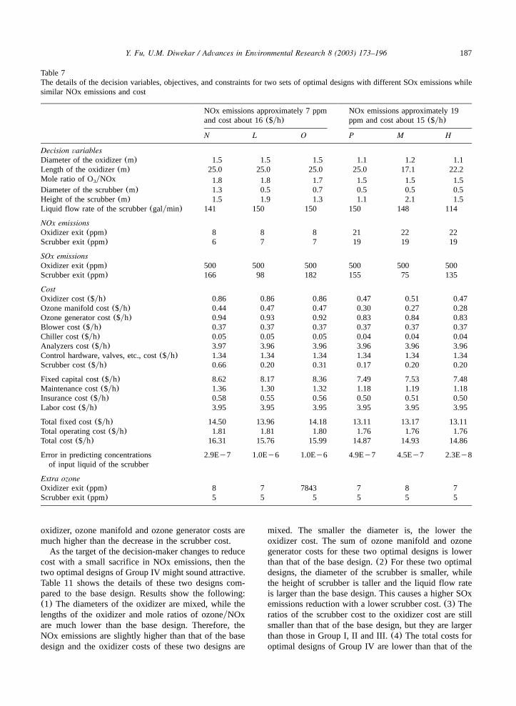
objectives, and constraints for two sets of optimaldesigns with different SOx emissions but similar NOxemissions and cost. The first set consists of three designs(N, L and O) with NOx emissions approximately 7ppm and cost approximately $16yh while design L hassignificantly less SOx emissions than N and O. Com-pared with N and O, Design L tends to use a smallerdiameter but a taller height of the scrubber and largerliquid flow rate, which help to remove more SOxemissions while keeping the scrubber cost in the samerange or lower than the other two. The similar phenom-ena occurs in the second set of optimal designs whichincludes three optimal designs(P, M and H) with NOxemissions approximately 19 ppm and cost approximately$15yh.Fig. 5 also shows that there are four optimal designs

(Group I) for which all objectives are better than thebase design, and these four designs are compared withthe base design in details in Table 8. Results show that(1) these four optimal designs tend to choose a largerdiameter, but similar length oxidizers, in order to reducemore NOx in the oxidizer than the base design. This


Fig. 5. Normalized objectives of the 104(the base design and 103 optimal designs) different designs for the case of the LTOprocess.

way, the oxidizer costs of optimal designs are higherthan that of the base design.(2) The mole ratios ofozoneyNOx for optimal designs are smaller than that ofthe base design, so that the extra ozone can be less thanthe limit of 5 ppm. This means that instead of usingmore ozone to reach higher NOx emissions, here thesefour optimal designs choose to use larger diameteroxidizers. (3) The diameter and the height of thescrubber are smaller, while the liquid flow rates arelarger than the base design, which help to reduce moreSOx emissions with a much lower scrubber cost.(4)The ratios of the scrubber cost to the oxidizer cost aremuch lower than that of the base design, which indicatesthat good designs spend more money on the oxidizerinstead of on the scrubber, but they still can obtainlower SOx emissions.(5) Total cost savings for thesefour optimal designs come from the difference betweenthe larger decrease in the scrubber cost and the smallerincrease of the oxidizer cost. Therefore, all four designsare good candidates if the decision-maker wants toimprove the base design in all objectives and satisfy theextra ozone constraint in the current case study.If the goal of the decision-maker is to see the potential

ability of the LTO process for the SOx emissionsremoval and heyshe is willing to sacrifice slightly in

cost over the base design, then the two optimal designsin Group II are better candidates. Table 9 shows thefollowing. (1) These two optimal designs also tend tochoose a larger diameter, but slightly shorter length ofthe oxidizer, in order to reduce more NOx in the oxidizerthan the base design. This way, the oxidizer costs ofoptimal designs are higher than that of the base design.(2) This has the same designs as of Group I, and themole ratios of ozoneyNOx for these two optimal designsare smaller than that of the base design, so that theextra ozone is less than the limit of 5 ppm in the currentcase study.(3) For all optimal designs in Group II, thediameters of the scrubber are smaller, but heights of thescrubber are taller and liquid flow rates are larger thanthose of the base design, which explains the higherreduction rate for the SOx emissions and lower scrubbercost.(4) The ratios of the scrubber cost to the oxidizercost are smaller than that of the base design and thoseof the designs in Group I. This also shows that gooddesigns spend more money on the oxidizer than on thescrubber and there is no need to significantly increasethe scrubber cost to remove more SOx emissions.(5)The total costs for these two optimal designs are a littlehigher than that of the base design since the rise in theoxidizer cost is higher than the cut in the scrubber cost.


Table 6The details of the decision variables, objectives, and constraints for three optimal designs with NOx emissions lower than 8 ppmand three other optimal designs with NOx emissions higher than 8 ppm

NOx emissions lower than 8(ppm) NOx emissions higher than 8(ppm)

B K L E M F




Cost (Costs18.51y0.405 NOx emissions,R s0.82)2

(Costs16.33y0.072 NOx emis-sions,R s0.98)2

Oxidizer cost($yh) 0.86 1.00 0.92 0.61 0.51 0.37Ozone manifold cost($yh) 0.44 0.49 0.47 0.30 0.27 0.22Ozone generator cost($yh) 0.97 0.94 0.93 0.85 0.84 0.80Blower cost($yh) 0.37 0.37 0.37 0.37 0.37 0.37Chiller cost($yh) 0.05 0.05 0.05 0.04 0.04 0.04Analyzers cost($yh) 3.96 3.96 3.96 3.96 3.96 3.96Control hardware, valves, etc., cost($yh) 1.34 1.34 1.34 1.34 1.34 1.34Scrubber cost($yh) 0.90 0.24 0.20 0.20 0.20 0.20



Error in predicting concentrations 1.00Ey06 2.20Ey7 1.0E–6 3.9Ey8 4.5Ey7 4.5Ey7of input liquid of the scrubber


When the decision-maker wants to reduce much moreNOx emissions and have greater SOx emissions removalthan the base design with more tolerance for costincreases, then the four optimal designs in Group III arebetter choices. The details of the base design and thesefour optimal designs are shown in Table 10. Resultsshow the following:(1) These four optimal designs usea larger diameter, and a similar length of the oxidizer,and a much higher mole ratio of ozoneyNOx in orderto reduce much more NOx emissions than the basedesign. In this way, the costs for the oxidizer, ozone

manifold, and ozone generator are much higher thanthose in the base design.(2) The diameter of thescrubber is smaller, the height is taller, and the liquidflow rate is larger than in the base design, whichexplains the higher reduction rate for the SOx emissionsand lower scrubber cost.(3) Similar to Group I and II,the ratios of the scrubber cost to the oxidizer cost forGroup III are much smaller than that of the base designdue to a higher removal rate of NOx emissions.(4)Total costs for these two optimal designs are muchhigher than the base design since the boosts in the


Table 7The details of the decision variables, objectives, and constraints for two sets of optimal designs with different SOx emissions whilesimilar NOx emissions and cost

NOx emissions approximately 7 ppmand cost about 16($yh)

NOx emissions approximately 19ppm and cost about 15($yh)

N L O P M H




CostOxidizer cost($yh) 0.86 0.86 0.86 0.47 0.51 0.47Ozone manifold cost($yh) 0.44 0.47 0.47 0.30 0.27 0.28Ozone generator cost($yh) 0.94 0.93 0.92 0.83 0.84 0.83Blower cost($yh) 0.37 0.37 0.37 0.37 0.37 0.37Chiller cost($yh) 0.05 0.05 0.05 0.04 0.04 0.04Analyzers cost($yh) 3.97 3.96 3.96 3.96 3.96 3.96Control hardware, valves, etc., cost($yh) 1.34 1.34 1.34 1.34 1.34 1.34Scrubber cost($yh) 0.66 0.20 0.31 0.17 0.20 0.20



Error in predicting concentrations 2.9Ey7 1.0Ey6 1.0Ey6 4.9Ey7 4.5Ey7 2.3Ey8of input liquid of the scrubber


oxidizer, ozone manifold and ozone generator costs aremuch higher than the decrease in the scrubber cost.As the target of the decision-maker changes to reduce

cost with a small sacrifice in NOx emissions, then thetwo optimal designs of Group IV might sound attractive.Table 11 shows the details of these two designs com-pared to the base design. Results show the following:(1) The diameters of the oxidizer are mixed, while thelengths of the oxidizer and mole ratios of ozoneyNOxare much lower than the base design. Therefore, theNOx emissions are slightly higher than that of the basedesign and the oxidizer costs of these two designs are

mixed. The smaller the diameter is, the lower theoxidizer cost. The sum of ozone manifold and ozonegenerator costs for these two optimal designs is lowerthan that of the base design.(2) For these two optimaldesigns, the diameter of the scrubber is smaller, whilethe height of scrubber is taller and the liquid flow rateis larger than the base design. This causes a higher SOxemissions reduction with a lower scrubber cost.(3) Theratios of the scrubber cost to the oxidizer cost are stillsmaller than that of the base design, but they are largerthan those in Group I, II and III.(4) The total costs foroptimal designs of Group IV are lower than that of the


Table 8The details of the decision variables, objectives, and constraints for four optimal designs(Group I) for which all objectives arebetter than the base design

Base design Group I in Fig. 5

A Q R S H

Decision variablesDiameter of the oxidizer(m) 0.8 1.0 1.0 1.1 1.1Length of the oxidizer(m) 24.4 22.2 25.0 22.2 22.2Mole ratio of O yNOx3 1.6 1.5 1.5 1.5 1.5Diameter of the scrubber(m) 0.9 0.5 0.5 0.5 0.5Height of the scrubber(m) 1.5 1.5 1.1 1.5 1.5Liquid flow rate of the scrubber(galymin) 85 138 150 114 114

NOx emissionsOxidizer exit(ppm) 23 23 22 22 22Scrubber exit(ppm) 20 20 20 20 19% decrease in NOx emissions than A – 0.7 2.3 3.8 5.2

SOx emissionsOxidizer exit(ppm) 500 500 500 500 500Scrubber exit(ppm) 191 115 155 135 135% decrease in SOx emissions than A – 39.6 19.1 29.5 29.5

CostOxidizer cost($yh) 0.27 0.43 0.44 0.45 0.47Ozone manifold cost($yh) 0.21 0.27 0.28 0.28 0.28Ozone generator cost($yh) 0.88 0.82 0.82 0.83 0.83Blower cost($yh) 0.37 0.37 0.37 0.37 0.37Chiller cost($yh) 0.04 0.04 0.04 0.04 0.04Analyzers cost($yh) 3.96 3.96 3.96 3.96 3.96Control hardware, valves, etc., cost($yh) 1.34 1.34 1.34 1.34 1.34Scrubber cost($yh) 0.41 0.19 0.17 0.19 0.19

Fixed capital cost($yh) 7.49 7.42 7.43 7.46 7.48Maintenance cost($yh) 1.18 1.17 1.17 1.17 1.18Insurance cost($yh) 0.50 0.50 0.50 0.50 0.50Labor cost($yh) 3.95 3.95 3.95 3.95 3.95

Total fixed cost($yh) 13.12 13.04 13.04 13.08 13.11Total operating cost($yh) 1.78 1.76 1.76 1.76 1.76Total cost($yh) 14.90 14.79 14.79 14.84 14.86% cost saving than A – 0.70 0.70 0.40 0.20

Ratio of scrubber costyoxidizer cost 1.50 0.43 0.40 0.41 0.40

Error in predicting concentrations 4.30Ey07 2.5Ey8 4.6Ey7 2.3Ey8 2.3Ey8of input liquid of the scrubber

Extra ozoneOxidizer exit(ppm) 13 7 7 7 7Scrubber exit(ppm) 9 5 5 5 5

base design, which is mainly due to the decreases inozone related and scrubber costs.In spite of the distinctive characteristics of the above

four groups, there are also some common elements thatcan be found. They are summarized in that good designstend to have(1) a larger diameter of the oxidizer, whichcan help to reduce more NOx emissions,(2) a smallerdiameter of the scrubber which can cut the scrubber

cost while reducing more SOx emissions,(3) a tallerscrubber which can also remove more SOx emissions,(4) a larger liquid flow rate which can reduce both SOxand NOx emissions, and(5) a smaller ratio of scrubbercostyoxidizer cost, which indicates the tradeoff betweenthe oxidizer and scrubber.It is worth re-emphasizing that the nonlinear, noncon-

vex nature of the problem can be used to choose designs


Table 9The details of the decision variables, objectives and constraints for two optimal designs(Group II) that have significantly lowerSOx emissions, similar NOx emissions and slighter higher cost than the base design

Base design Group II in Fig. 5

A M E

Decision variablesDiameter of the oxidizer(m) 0.8 1.2 1.4Length of the oxidizer(m) 24.4 17.1 13.5Mole ratio of O yNOx3 1.6 1.5 1.5Diameter of the scrubber(m) 0.9 0.5 0.5Height of the scrubber(m) 1.5 2.1 2.0Liquid flow rate of the scrubber(galymin) 85 148 141

NOx emissionsOxidizer exit(ppm) 23 22 20Scrubber exit(ppm) 20 19 18% decrease in NOx emissions than A – 6.8 12.8

SOx emissionsOxidizer exit(ppm) 500 500 500Scrubber exit(ppm) 191 75 79% decrease in SOx emissions than A – 60.6 58.5

CostOxidizer cost($yh) 0.27 0.51 0.61Ozone manifold cost($yh) 0.21 0.27 0.30Ozone generator cost($yh) 0.88 0.84 0.85Blower cost($yh) 0.37 0.37 0.37Chiller cost($yh) 0.04 0.04 0.04Analyzers cost($yh) 3.96 3.96 3.96Control hardware, valves, etc., cost($yh) 1.34 1.34 1.34Scrubber cost($yh) 0.41 0.20 0.20

Fixed capital cost($yh) 7.49 7.53 7.66Maintenance cost($yh) 1.18 1.19 1.21Insurance cost($yh) 0.50 0.51 0.51Labor cost($yh) 3.95 3.95 3.95

Total fixed cost($yh) 13.12 13.17 13.32Total operating cost($yh) 1.78 1.76 1.77Total cost($yh) 14.90 14.92 15.08% cost saving than A – y0.20 y1.20

Ratio of scrubber costyoxidizer cost 1.50 0.40 0.33

Error in predicting concentrations 4.30Ey07 4.50Ey7 3.90Ey8of input liquid of the scrubber

Extra ozoneOxidizer exit(ppm) 13 8 7Scrubber exit(ppm) 9 5 5

that have a much better SOx emissions reduction rateand have similar NOx emissions and cost compared tothe designs nearby whenever this is possible(shown inFig. 4). Thus far, the original 103 optimal designs havebeen screened to a reasonable number of the potentiallyattractive designs in four different groups, which willhelp the decision-maker to identify hisyher final choice.

3.5.5. Multiple regression analysisAs all 103 designs were found by the nonlinear

optimizer that have minimal cost according to thedifferent targets for the NOx and SOx emissions, itwould be nice if some overall approximate quantitativeunderstanding can be gained by using some statisticalanalysis tools. Here we choose to identify the key


Table 10The details of the decision variables, objectives and constraints for four optimal designs(Group III) that have significantly lowerNOx emissions and lower SOx emissions but a higher cost than the base design

Base design Group III in Fig. 5

A C T L K

Decision variablesDiameter of the oxidizer(m) 0.8 1.5 1.5 1.5 1.5Length of the oxidizer(m) 24.4 22.1 25.0 25.0 25.0Mole ratio of O yNOx3 1.6 1.7 1.7 1.8 1.8Diameter of the scrubber(m) 0.9 0.5 0.5 0.5 0.6Height of the scrubber(m) 1.5 2.2 1.9 1.9 1.6Liquid flow rate of the scrubber(galymin) 85 150 150 150 150

NOx emissionsOxidizer exit(ppm) 23 10 9 8 6Scrubber exit(ppm) 20 9 8 7 6% decrease in NOx emissions than A – 57.5 61.2 66.6 72.6

SOx emissionsOxidizer exit(ppm) 500 500 500 500 500Scrubber exit(ppm) 191 73 87 98 122% decrease in SOx emissions than A – 61.9 54.6 48.8 36.3

CostOxidizer cost($yh) 0.27 0.82 0.86 0.92 1.00Ozone manifold cost($yh) 0.21 0.41 0.44 0.47 0.49Ozone generator cost($yh) 0.88 0.92 0.92 0.93 0.94Blower cost($yh) 0.37 0.37 0.37 0.37 0.37Chiller cost($yh) 0.04 0.04 0.04 0.05 0.05Analyzers cost($yh) 3.96 3.97 3.96 3.96 3.96Control hardware, valves, etc., cost($yh) 1.34 1.34 1.34 1.34 1.34Scrubber cost($yh) 0.41 0.20 0.20 0.20 0.24

Fixed capital cost($yh) 7.49 8.08 8.13 8.23 8.40Maintenance cost($yh) 1.18 1.27 1.28 1.30 1.32Insurance cost($yh) 0.50 0.54 0.55 0.55 0.56Labor cost($yh) 3.95 3.95 3.95 3.95 3.95

Total fixed cost($yh) 13.12 13.83 13.91 14.03 14.23Total operating cost($yh) 1.78 1.80 1.80 1.81 1.81Total cost($yh) 14.90 15.63 15.71 15.83 16.03% cost saving than A – y4.90 y5.40 y6.30 y7.60

Ratio of scrubber costyoxidizer cost 1.50 0.24 0.23 0.21 0.24

Error in predicting concentrations 4.3Ey07 1.0Ey06 4.1Ey7 6.3Ey7 2.2Ey7of input liquid of the scrubber

Extra ozoneOxidizer exit(ppm) 13 7 7 7 7Scrubber exit(ppm) 9 5 5 5 5

decision variables that affect the different objectives andto analyze the relationship among the three objectivesusing the multiple regression analysis method in MIN-ITAB. Because of the nonlinear nature of the problem,some higher-order terms are included as needed.Table 12 shows the following:(1) The total cost is

affected by six decision variables, which are the diam-eter of the oxidizer(x ), the length of the oxidizer(x ),1 2

the mole ratio of ozoneyNOx (x ), the diameter of the3

scrubber(x ), the height of the scrubber(x ), and the4 5

liquid flow rate (x ). (2) The NOx emissions are6

generally influenced by four of the decision variablesx , x , x and x , but x and x have less effect thanx1 3 4 6 4 6 1

and x . (3) Decision variablesx , x and x are the3 4 5 6

important variables for the SOx emissions, which iswhy the SOx reduction does not show a significant


Table 11The details of the decision variables, objectives, and constraints for two optimal designs(Group IV) that have much lower cost andSOx emissions and slightly higher NOx emissions than the base design

Base design Group IV in Fig. 4

A U F

Decision variablesDiameter of the oxidizer(m) 0.8 0.7 1.1Length of the oxidizer(m) 24.4 15.7 13.4Mole ratio of O yNox3 1.6 1.3 1.4Diameter of the scrubber(m) 0.9 0.5 0.5Height of the scrubber(m) 1.5 2.0 2.0Liquid flow rate of the scrubber(galymin) 85 147 141

NOx emissionsOxidizer exit(ppm) 23 33 28Scrubber exit(ppm) 20 29 24% decrease in NOx emissions than A – y41.4 y17.3

SOx emissionsOxidizer exit(ppm) 500 500 500Scrubber exit(ppm) 191 71 80% decrease in SOx emissions than A – 63.1 58.3

CostOxidizer cost($yh) 0.27 0.17 0.37Ozone manifold cost($yh) 0.21 0.16 0.20Ozone generator cost($yh) 0.88 0.76 0.80Blower cost($yh) 0.37 0.37 0.37Chiller cost($yh) 0.04 0.03 0.04Analyzers cost($yh) 3.96 3.96 3.96Control hardware, valves, etc., cost($yh) 1.34 1.34 1.34Scrubber cost($yh) 0.41 0.20 0.20

Fixed capital cost($yh) 7.49 7.00 7.27Maintenance cost($yh) 1.18 1.10 1.15Insurance cost($yh) 0.50 0.47 0.49Labor cost($yh) 3.95 3.95 3.95

Total fixed cost($yh) 13.12 12.52 12.85Total operating cost($yh) 1.78 1.73 1.74Total cost($yh) 14.90 14.28 14.59% cost saving than A – 4.10 2.00

Ratio of scrubber costyoxidizer cost 1.50 1.15 0.54

Error in predicting concentrations 4.3Ey07 4.4Ey7 4.5Ey7of input liquid of the scrubber

Extra ozoneOxidizer exit(ppm) 13 7 7Scrubber exit(ppm) 9 5 5

impact on the NOx removal asx , x and x do not4 5 6

considerably affect the NOx emissions.(4) The SOxemissions appear to have a less significant effect on thecost than the NOx emissions because the absolutecoefficient of the SOx emissions(0.000896) is muchless than that of the NOx emissions(0.0745). However,it worthy of mention that because of the nonlinear,nonconvex nature of the problem(also see Fig. 4), on

average, the higher SOx emissions tend to have a highercost which tends to choose designs that have lower SOxemissions. Therefore, it is possible to explore the non-linear relationship between the cost and the SOx emis-sions to find designs that have better SOx emissionsreduction with similar NOx emission and cost as dis-cussed earlier.(5) The NOx reduction is the key factorto increase cost, on average, the cost increases by


Table 12Multiple regression analysis results for the 103 designs of the case study

Response The regression equation R (%)2a

Cost Z s11.9q1.23x q0.00709x q0.647x q0.863x q0.0275x q0.000361x1 1 2 3 4 5 6 99.50NOx emissions Z s63.5y12.5x y19.2x y0.827x y0.018x2 1 3 4 6 98.90SOx emissions Z s497q379x y230x y3.73x y161x q49.1x q0.0116x2 2 2

3 4 5 6 4 5 6 92.90

Cost Z s16.2y0.0745Z q0.000896Z1 2 3 95.40

R is the sample multiple coefficient of determination.R s0 implies a complete lack of fit of the model to the data, andR sa 2 2 2

1 implies a perfect fit, with the model passing through every data point(Mendenhall and Sincich 1989).

Fig. 6. Comparison the 104 designs(the base design and 103 optimal designs) at two different temperature.

$0.0745yh to reduce the NOx emissions by 1 ppm withthe similar SOx emissions in this case study. Becauseof the nonlinear nonconvex nature of the problem, thedecision-maker is recommended to check the detaileddiscussions earlier for any particular range of designs.

3.5.6. Higher temperature impactsAs discussed in Section 3.1, the base design has

much lower NOx, SOx, and extra ozone emissions witha small increase in cost when temperature increases.Fig. 6 shows the different performances and cost chang-

es at two different temperatures, the temperature of thecurrent case study(78 8F) and a slightly higher temper-ature (125 8F), for the other 103 optimal designsobtained in the current case study. Fig. 6 shows thefollowing: (1) For all designs obtained in the currentcase study, the NOx emissions, SOx emissions, andextra ozone at a higher temperature(125 8F) are muchlower than those at the current temperature for the casestudy (78 8F) with only a minor increase in cost. Thisconfirms that the temperature is a very important oper-ating variable that is relatively easy to control while


having a significant positive impact on the performanceof the LTO process.(2) The difference in the NOxemissions between higher and lower temperatures reduc-es when the NOx emissions become lower. This meansdesigns with relatively higher NOx emissions at a lowertemperature(78 8F) have much more improvement inthe NOx emissions removal when the temperature is atthe higher level(125 8F). (3) SOx emissions still jumplocally at higher temperatures when NOx emissionsreduce, but the scale is much smaller than that at thelower temperature.(4) For the specified NOx and SOxemissions targets we now can choose much cheaperdesigns if we operate the LTO process at 1258F insteadof 78 8F. (5) At 125 8F the ozone slips are less than 1ppm for all 103 optimal designs instead of 5 ppm at 788F, which are better than the base design because thereis still approximately 2 ppm extra ozone for the basedesign operating at 1258F.

3.5.7. Brief summaryIn summary, this case study has demonstrated that

the efficient MINSOOP algorithm provides a valuableand systematic tool for designing the best availablecontrol technology(BACT) for NOx removal. It offersmultiple Pareto optimal designs that cover the wholePareto set in an efficient and uniform way and presentsabundant insight information approximately the multiob-jective problem at hand. The nonlinear nature of theLTO process can be explicitly captured by these designs,which provides many opportunities to eliminate baddesigns and to promote designs that have lower emis-sions and lower cost. The impact of NOx removal tothe system cost is much higher than that of the SOxreduction. Therefore, the multiobjective optimizationapproach can provide designs that have a similar NOxreduction rate, but have much better SOx removal witha very trivial change of the cost. The effects of keydecision variables on different objectives and the rela-tionship among objectives can also be analyzed fromthese Pareto optimal designs, and some heuristic knowl-edge can be gained as well. In general, higher temper-atures help to reduce more NOx, SOx, and extra ozoneemissions with little increase in cost.The total cost has been found to increase approxi-

mately linearly as the NOx emissions decrease, whileSOx emissions can be reduced considerably withoutsignificant increases of the NOx emissions and costusing the nonlinear nonconvex nature of the problem.All six design and operating variables have been provento be important variables to cost, while only four ofthem—the diameter of the oxidizer, the mole ratio ofozoneyNOx, the diameter of the scrubber and the liquidflow rate affect NOx emissions considerably. Only threedecision variables, the diameter of the scrubber, theheight of the scrubber, and the liquid flow rate are thekey variables to the SOx emissions. The 103 Pareto

optimal designs obtained have been screened to fourgroups with 12 designs, which are the most attractivedesigns according to the possible different targets of thedecision-maker. Some common elements for the gooddesigns, such as a larger diameter oxidizer, a smallerdiameter and a taller scrubber, a larger liquid flow rate,and a smaller ratio of scrubber cost to oxidizer cost,have also been identified. The current case study isdesigned for a very low temperature(78 8F), however,at higher temperatures()78 8F), the process perform-ances are better than those at the lower temperaturecondition with only trivial increase in cost for the sameoptimal design.

4. Conclusions

In this paper, the LTO process model has beenincorporated in a multiobjective problem to obtainminimum cost and minimum emissions designs. Themultiobjective optimization framework for the LTOprocess allows for solving the modeling and optimiza-tion problems simultaneously. Results have establishedthat the new and efficient MINSOOP algorithm is amuch better tool than the traditional design of experi-ment or the single objective optimization methodsbecause it optimizes the multiple decision variables atthe same time using the optimizer instead of changingthem one-at-a-time, and it offers multiple Pareto optimaldesigns instead of the dominated designs or only asingle optimal design. As a result, the decision-makerwill have more freedom to choose the final designamong multiple optimal designs according to hisyherimplicit value function. The 3D surface and contourplots for the approximate Pareto set can provide explicitinformation approximately the characteristics of theproblem and the tradeoff information among differentobjectives to support the decision-making.The general multiobjective optimization framework

of this study has been shown to be a valuable tool fordesign engineers for redesigning this BACT system tomake it cost efficient while keeping its advantage ofvery low levels of all pollutant emissions. This can helpto promote the market for this pollution control tech-nology to reduce the high levels of NOx and SOxemissions.

Acknowledgments

The authors would like to acknowledge the researchfunding from the Environmental Protection Agency andPennsylvania Infrastructure Technology Alliance Grant(PITA Year 3). We also want to thank Dr NareshSuchak, BOC Gases, for providing insights into theprocess and cost models for this work.


Nomenclature

ACFM flow rate of input flue gas in cubic feetper minute

CROSSA cross-sectional area of the oxidizer(m )2

C –C1 17 model parametersC_ANAL cost of analyzers, conditioners and

measuring instrument($)C_BLOWER cost of blower($)C_CC cost of chemical($yh)C_CCF cost of installed equipment plus one

year of oxygen cost($)C_CHILLER cost of chiller($)C_CONTROL cost of control hardware, valves, etc.

($)C_DRIVE cost of drive for blower($yh)C_ELEC cost of electricity($yh)C_FCC total capital cost($yh)C_FAN cost of fan for blower($yh)C_FIXED fixed costs($)C_IEC installed equipment cost($)C_INSUR insurance costs($yh)C_LBHR hourly labor costs per worker($yh)C_LABOR labor costs($yh)C_MAIN hourly maintenance costs($yh)C_MOC cost of constructed material($ylb)C_O2 cost of oxygen($yh)C_O3GEN cost of ozone generation equipment

($)C_O3MAN cost of ozone manifold($)C_OXY cost of the oxidation duct($)C_PACK cost of scrubber packing($ym )3

C_PEC cost of equipments($)C_PW cost of process water($yh)C_SC cost of scrubber($)C_TCC total capital cost($)C_TFC total fixed cost($yh)C_TOC total operating cost($yh)C_TOTAL total cost of the LTO process($yh)C_UO2 cost of unit oxygen(centsy100 SCF)C_UKW cost of unit of electricity(centsykW)C_UCC cost of unit chemical cost($ylb)C_UPW cost of unit process water

($y1000 gal)CWTHR chemical consumed in weightD_DIA diameter of the oxidation duct(m)DELTAP differential pressure head across the

fanDT_CHG delta T in chilled waterEKW_BLOWER power required to blower

(kW hyday)EKW_CH power required to chiller(kW hyday)EKW_CTRL power Consumption for control and

analyzers(kW h)EKW_O3 power required in ozone generation

(kW hyday)EKW_SC power consumption by scrubber

pumps(kW h)

EKW_TOTAL total power consumption(kW h)FG_LBS factor coefficient of laborFLOW_CW flow of chilled water(galymin)F_CONT cost factor for contingency feeF_ENGF cost factor for engineering feesF_GF cost factor for general facilitiesF_INSTAL cost factor for installationF_INSUR cost factor for insurance feesF_INT interest for capital recovery factorHMAX the maximum height of the scrubber

(m)HR_YRS number of hours of operation per

year(hyyear)KW_BLOWER power required in blower(kW h)LMAX the total length of the oxidizer(m)NETA_F fan efficiencyNYRS number of years to be usedO2_LBS oxygen required(lbyh)O3LBS ozone required(lbyday)OXY_VOL volume of the oxidation duct(ft )3

OXY_WT oxidizer weight(lb)PWGALS process water used(galyh)REF_TON tons of refrigeration(tons)RT residence time of the oxidizer(s)SC_CRA cross-sectional area of the scrubber

(m )2

SC_DIA scrubber diameter(m)SC_WT scrubber weight(lb)SG_MOC specific gravity of material of

constructionSPGR_CW specific gravity of chilled waterTHKOG given thickness of oxidizer(m)THK_SCG given thickness of the scrubber(m)TONS_CHL refrigeration required(tons)VOL_PACK packing volume(m )3

VOL_SCR scrubber volume(m )3

WT_O3 percent of O by weight3

Appendix A: Cost model for the LTO process

CROSSAs3.1416y4*D DIA*D DIA (A1)

UOXY VOLsCROSSA LMAX (A2)

OXY WTU U U Us3.1416 D DIA LMAX THKOG SG MOC

(A3)

U U UUC OXYs(OXY WT C MOC) C 2 (A4)1

C O3MANsC qCROSSAyC (A5)2 3


UC O3GENsO3LBS C (A6)4

U UKW BLOWERsACFM C DELTAPyNETA F5

(A7)

U UUC DRIVEsC KW BLOWER 0.4073 (A8)6

U UUC FANsC ACFM 0.64 (A9)7

C BLOWERsC DRIVEqC FAN (A10)

UTONS CHLsO3LBS 0.059524 (A11)

UC CHILLERsC TONS CHL (A12)8

UC ANALsC qC O3LBS9 10

U UUyC O3LBS 2 (A13)11

U UUC CONTROLsyC ACFM 212

UqC ACFMqC13 14

UqC O3LBS (A14)15

U USC CRAs3.1416 SC DIA SC DIA (A15)

UVOL SCRsHMAX SC CRA (A16)

U USC WTs3.1416 SC DIAU U UHMAX THK SCy12 62.5 SG MOC (A17)

U U UUC SCs(SC WT C MOC) 1.25 2UqVOL SCR C PACK (A18)

C PECsC OXYqC O3MANqC O3GENqC BLOWERqC CHILLERqC ANALqC CONTROLqC SC (19)

UC IECsC PEC (1qF INSTAL) (A20)

UC TCCsC IEC (1qF GFqF ENGFqF CONTqF INSUR) (A21)

UC MAINs0.03 C IECyHR YRS (A22)

UC INSURsF INSUR C TCCyHR YRS (A23)

UC LABORsC LBHR (C16

U UUq7 (FG LBSyC ) 0.86) (A24)17

UC CCFsF INT ((1UUqF INT)) NYRS)y((1UUqF INT) NYRSy1) (A25)

UC FCCs(C TCC C CCF)yHR YRS (A26)

C TFCsC FCCqC MAINqC INSURqC LABOR (A27)

UEKW O3sO3LBS 6.0 (A28)

FLOW CWsO3LBSy7.5 (A29)

REF TONU U U UsFLOW CW DT CHG 8.33 24 60y12000y24

(A30)

U UUEKW CHs((1.2933 REF TON)U(y0.0619)) REF TON (A31)

U U UEKW SCs(HMAX 60 18y3.78) 60U USPGR CW 0.746y3960y0.7y0.9 (A32)

EKW TOTALs(EKW O3qEKW CH)y24qEKW BLOWERqEKW SCqEKW CTRL (A33)

UC ELECsEKW TOTAL C UKWy100 (A34)


O2 LBSsO3LBSy(WT O3Gy100) (A35)

UC O2sO2 LBSy24y12.08 C UO2y100y100(A36)

UC PWsPWGALS C UPWy1000 (A37)

UC CCsCWTHR C UCC (A38)

C TOCsC ELECqC O2qC PWqC CC (A39)

C TOTALsC TFCqC TOC (40)

References

Cohon, J.L., 1978. Multiobjective Programming and Planning.Academic Press, Inc, New York.

Cooper, C., 1998. EPA Imposes 28% NOx Cut by 2007,Chemical Engineering, November: 54.

Fu, Y., Diwekar, U., Suchak N., Rohrer W., 1999. Modelingthe Best Available Control Technology: Numerical Difficul-

ties and the Optimization Framework. Paper presented atthe AIChE Annual Meeting, Dallas, TX.

Fu, Y., Diwekar, U., Suchak, N., 2000. Optimization frame-work for modeling the low temperature NOx reductionprocess. Adv. Environ. Res. 3, 424–438.

Fu, Y., 2000. Ph.D. dissertation, Process Design for theEnvironment: A Multiobjective Optimization Framework.Department of Civil and Environmental Engineering, Car-negie Mellon University, Pittsburgh, PA 15213.

Fu, Y., Diwekar, U. 2003 An Efficient Sampling Approach toMulti-objective Optimization, to appear in Annals of OR.

Haimes, Y.Y., Lasdon, L.S., Wismer, D.A., 1971. On a bicri-terion formulation of the problems of integrated systemidentification and system optimization. IEEE Trans. Syst.,Man, Cybernetics 1, 296–297.

Iman, R.L., Shortencarier, M.J., 1984. AFORTRAN77 Programand User’s Guide for Generation of Latin Hypercube andRandom Samples for Use with Computer Models, NUREG/CR-3624, SAND83-2365, 1984, Sandia National Laborato-ries, Albuquerque, NM.

Kalagnanam, J.R., Diwekar, U.M., 1997. An efficient samplingtechnique for off-line quality control. Technometrics 39,308–319.

Mendenhall, W., Sincich, T., 1989. A Second Course inBusiness Statistics: Regression Analysis. third ed.. DellenPublishing Company, San Francisco, CA.

Suchak, N.J. May 2000, personal communication.Zeleny, M., 1982. Multiple Criteria Decision Making.McGraw-Hill, Inc, New York.

Cost effective environmental control technology for utilities

Documents

Transcript of Cost effective environmental control technology for utilities