Cost Curves for Abstaining Classifiers

Caroline C. Friedel Caroline.Friedel@bio.ifi.lmu.de

Institut fur Informatik, Ludwig-Maximilians-Universitat Munchen, Amalienstr. 17, 80333 Munchen, Germany

Ulrich Ruckert rueckert@in.tum.deStefan Kramer kramer@in.tum.de

Institut fur Informatik/I12, Technische Universitat Munchen, Boltzmannstr. 3, 85748 Garching b. Munchen,Germany

Abstract

We present abstention cost curves, a newthree-dimensional visualization technique toillustrate the strengths and weaknesses of ab-staining classifiers over a broad range of costsettings. The three-dimensional plot showsthe minimum expected cost over all ratios offalse-positive costs, false-negative costs andabstention costs. Generalizing Drummondand Holte’s cost curves, the technique allowsto visualize optimal abstention settings andto compare two classifiers in varying cost sce-narios. Abstention cost curves can be usedto answer questions different from those ad-dressed by ROC-based analysis. Moreover, itis possible to compute the volume under theabstention cost curve (VACC) as an indicatorof the classifier’s performance across all costscenarios. In experiments on UCI datasetswe found that learning algorithms exhibit dif-ferent “patterns of behavior” when it comesto abstention, which is not shown by othercommon performance measures or visualiza-tion techniques.

1. Introduction

In many application areas of machine learning it isnot sensible to predict the class for each and everyinstance, no matter how uncertain the prediction is.Instead, classifiers should have the opportunity to ab-stain from risky predictions under certain conditions.Our interest in abstaining classifiers is motivated byspecific applications, for instance in chemical risk as-

Appearing in Proceedings of the ICML 2006 workshop onROC Analysis in Machine Learning, Pittsburgh, PA, 2006.Copyright 2006 by the author(s)/owner(s).

sessment, where it is considered harmful to predictthe toxicity or non-toxicity of a chemical compoundif the prediction is weak and not backed up by suffi-cient training material.

Abstaining classifiers can easily be derived from non-abstaining probabilistic or margin-based classifiers bydefining appropriate thresholds which determine whento classify and when to refrain from a prediction. Thelower and upper thresholds, within which no classi-fications are made, constitute a so-called abstentionwindow (Ferri et al., 2004). Making use of absten-tion windows, a recent approach based on ROC anal-ysis (Pietraszek, 2005) derives an optimal abstainingclassifier from binary classifiers. In this approach thethresholds can be determined independently of eachother from the convex hull of ROC curves. However,ROC-based approaches assume at least known mis-classification costs. Moreover, classifiers and optimalabstention thresholds cannot be compared directly fora range of possible cost matrices, as it is usually donein cost curves (Drummond & Holte, 2000).

In this paper, we propose an alternative approach toROC-based analysis of abstaining classifiers based oncost curves. The advantage of cost curves is that cost-related questions can be answered more directly, andthat the performance over a range of cost scenarios canbe visualized simultaneously. The proposed general-ization of cost curves plots the optimal expected costs(the z-axis) against the ratio of false positive costs tofalse negative costs (the x-axis) and the ratio of ab-stention costs to false negative costs (the y-axis). Thefundamental assumption is that abstention costs canbe related to misclassification costs. As pointed out byother authors (Pietraszek, 2005), unclassified instancesmight take the time or effort of other classifiers (Ferriet al., 2004), or even human experts. Another sce-nario is that a new measurement has to be made for

Cost Curves for Abstaining Classifiers

the instance to be classified. Thus, abstention costslink misclassification costs with attribute costs. Con-sequently, the setting is in a sense related to activelearning (Greiner et al., 2002). Along those lines, wealso assume that abstention costs are the same inde-pendently of the true class: Not knowing the class, theinstances are handled in the very same way.

We devised a non-trivial, efficient algorithm for com-puting the three-dimensional plot in time linear in theexamples and in the number of grid points (Friedel,2005). The algorithm takes advantage of dependen-cies among optimal abstention windows for differentcost scenarios to achieve its efficiency. However, thefocus of this paper is not on the algorithm, but onactual abstention cost curves of diverse classifiers onstandard UCI datasets. We present abstention costcurves as well as “by-products”, showing the absten-tion rates and the location of the abstention window(the lower and upper interval endpoints). Moreover, anew aggregate measure, the volume under the absten-tion cost curve (VACC), is presented. VACC is relatedto the expected abstention costs, if all cost scenariosare equally likely.

2. Abstaining in a Cost-SensitiveContext

Before going into detail, we need to specify some ba-sic concepts and introduce the overall setting. First ofall, we assume that a classifier Cl has been induced bysome machine learning algorithm. Given an instancex taken from an instance space X , this classifier as-signs a class label y(x) taken from the target classY = {P,N}, where P denotes the positive class andN the negative class. To avoid confusion, we use cap-ital letters for the actual class and lowercase lettersfor the labels assigned by the classifier. We wouldnow like to analyze this classifier on a validation setS = {s1, s2, . . . , sr} containing r instances with classes{y1, y2, . . . , yr}. As argued in the work on ROC curves(e.g. in (Provost & Fawcett, 1998)), it can make senseto use a different sampling bias for the training setthan for the validation set. In this case, the classprobabilities in the validation set might differ fromthe class probabilities of the training set or the trueclass probabilities. Thus, we do not explicitly assume,that the validation set shows the same class distribu-tion as the training set, even though this is the casein many practical applications. However, we demandthat the classifier outputs the predicted class label aswell as some confidence score for each instance in thevalidation set. For simplicity we model class label andconfidence score as one variable, the margin. The mar-

gin m(s) of an instance s is positive, if the predictedclass is p and negative otherwise. The absolute valueof the margin is between zero and one and gives someestimate of the confidence in the prediction. Thus, themargin m(s) of an instance s ranges from -1 (clearlynegative) over 0 (equivocal) to +1 (clearly positive).

Applying the classifier to the validation set, yields asequence of r (not necessarily distinct) margin valuesM = (m(s1),m(s2), . . . ,m(sr)). Sorting this sequencein ascending order yields a characterization of the un-certainty in the predictions. The certain predictionsare located at the left and right end of the sequenceand the uncertain ones somewhere in between. Basedon the information in this sequence one can then al-low the classifier Cl to abstain for instances with mar-gin values between a lower threshold l and an upperthreshold u. Any such ordered pair of thresholds con-stitutes an abstention window a := (l, u). A specificabstaining classifier is defined by an abstention win-dow a and its prediction on an instance x is given as

π(a, x) =

p if m(x) ≥ u⊥ if l < m(x) < un if m(x) ≤ l

(1)

where ⊥ denotes “don’t know”.

As both the upper and lower threshold of an absten-tion window are real numbers, the set of possible ab-stention windows is uncountably infinite. Therefore,we have to restrict the abstention windows consideredin some way. If we are given the margin values asa sorted vector (m1, . . . ,mk) of distinct values – i.e.,m1 < · · · < mk – it is sensible to choose the thresholdsjust in between two adjacent margin values. To modelthis, we define a function v : {0, . . . , k} → R whichreturns the center of the margin with index i and thenext margin to the right. We extend the definition ofv to the case where i < 1 or i = k to allow for absten-tion windows that are unbounded on the left or on theright:

v(i) =

mi+mi+1

2 if 1 ≤ i < k−∞ if i = 0+∞ if i = k.

(2)

Note that the original margin sequence may containthe same margin value more than once, but v is de-fined only on the k ≤ n distinct margin values. Theset of abstention windows A(Cl) for a classifier Cl isthen A(Cl) := {(v(i), v(j))|0 ≤ i ≤ j ≤ k}. Wherethe classifier is clear from the context, we omit it anddenote the set just by A.

The performance of an abstention window is assessedin terms of expected cost on the validation set. Tocalculate this, we need information about the costs

Cost Curves for Abstaining Classifiers

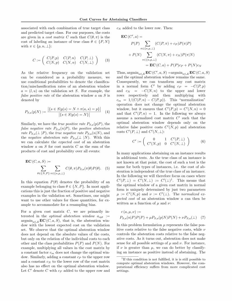
associated with each combination of true target classand predicted target class. For our purposes, the costsare given in a cost matrix C such that C(θ, π) is thecost of labeling an instance of true class θ ∈ {P,N}with π ∈ {p, n,⊥}:

C :=(

C(P, p) C(P, n) C(P,⊥)C(N, p) C(N,n) C(N,⊥)

)(3)

As the relative frequency on the validation setcan be considered as a probability measure, weuse conditional probabilities to denote the classifica-tion/misclassification rates of an abstention windowa = (l, u) on the validation set S. For example, thefalse positive rate of the abstention window a on S isdenoted by

PS,a(p|N) :=

∣∣{s ∈ S|y(s) = N ∧ π(a, s) = p}∣∣∣∣{s ∈ S|y(s) = N}

∣∣ (4)

Similarly, we have the true positive rate PS,a(p|P ), thefalse negative rate PS,a(n|P ), the positive abstentionrate PS,a(⊥ |P ), the true negative rate PS,a(n|N), andthe negative abstention rate PS,a(⊥ |N). With thiswe can calculate the expected cost of an abstentionwindow a on S for cost matrix C as the sum of theproducts of cost and probability over all events:

EC (C, a, S) :=∑θ∈{N,P}

∑π∈{n,p,⊥}

C(θ, π)PS,a(π|θ)P (θ). (5)

In this equation P (θ) denotes the probability of anexample belonging to class θ ∈ {N,P}. In most appli-cations this is just the fraction of positive and negativeexamples in the validation set. Sometimes, one mightwant to use other values for those quantities, for ex-ample to accommodate for a resampling bias.

For a given cost matrix C, we are primarily in-terested in the optimal abstention window aopt :=argmina∈A EC (C, a, S), that is, the abstention win-dow with the lowest expected cost on the validationset. We observe that the optimal abstention windowdoes not depend on the absolute values of the costs,but only on the relation of the individual costs to eachother and the class probabilities P (P ) and P (N). Forexample, multiplying all values in the cost matrix bya constant factor cm does not change the optimal win-dow. Similarly, adding a constant cP to the upper rowand a constant cN to the lower row of the cost matrixalso has no effect on the optimal abstention window.Let C ′ denote C with cP added to the upper row and

cN added to the lower row. Then:

EC (C ′, a) =

P (P )∑

π∈{n,p,⊥}

(C(P, π) + cP )P (π|P )

+ P (N)∑

π∈{n,p,⊥}

(C(N,π) + cN )P (π|N)

= EC (C, a) + P (P )cP + P (N)cN

Thus, argmina∈A EC (C ′, a, S) =argmina∈A EC (C, a, S)and the optimal abstention window remains the same.Consequently, we can transform any cost matrixin a normal form C ′ by adding cP = −C(P, p)and cN = −C(N,n) to the upper and lowerrows respectively and then multiplying withcm = 1/(C(P, n) − C(P, p)). This “normalization”operation does not change the optimal abstentionwindow, but it ensures that C ′(P, p) = C ′(N,n) = 0and that C ′(P, n) = 1. In the following we alwaysassume a normalized cost matrix C ′ such that theoptimal abstention window depends only on therelative false positive costs C ′(N, p) and abstentioncosts C ′(P,⊥) and C ′(N,⊥):

C ′ :=(

0 1 C ′(P,⊥)C ′(N, p) 0 C ′(N,⊥)

)(6)

In many applications abstaining on an instance resultsin additional tests. As the true class of an instance isnot known at that point, the cost of such a test is thesame for both types of instances, i.e. the cost of ab-stention is independent of the true class of an instance.In the following we will therefore focus on cases whereC ′(P,⊥) = C ′(N,⊥) := C ′(⊥)1. This means thatthe optimal window of a given cost matrix in normalform is uniquely determined by just two parametersµ := C ′(N, p) and ν := C ′(⊥). The normalized ex-pected cost of an abstention window a can then bewritten as a function of µ and ν:

c (a, µ, ν) :=PS,a(n|P )P (P ) + µPS,a(p|N)P (N) + νPS,a(⊥) (7)

In this problem formulation µ represents the false pos-itive costs relative to the false negative costs, while νcontrols the abstention costs relative to the false neg-ative costs. As it turns out, abstention does not makesense for all possible settings of µ and ν. For instance,if ν is greater than µ, we can do better by classify-ing an instance as positive instead of abstaining. The

1If this condition is not fulfilled, it is is still possible tocompute optimal abstention windows. However, the com-putational efficiency suffers from more complicated costsettings.

Cost Curves for Abstaining Classifiers

following lemma quantifies this phenomenon. For thesake of simplicity, we use the fractions of positive andnegative instances in the validation set for P (P ) andP (N). Therefore, we can determine PS,a(n|P )P (P ),PS,a(p|N)P (N) and PS,a(⊥) by counting the occur-rences of each event and then dividing by the numberof instances r.

Lemma 1. Let S, µ and ν be defined as before. Ifν > µ

1+µ , the optimal abstention window aopt is empty,i.e. lopt = uopt (proof omitted).

3. Cost Curves for AbstainingClassifiers

If the cost matrix and the class probabilities in a learn-ing setting are known exactly, one can determine theoptimal abstention window aopt simply by calculat-ing the expected costs for all windows. However, formost applications costs and class distributions are un-certain and cannot be determined exactly. In such asetting one would like to assess the performance of anabstaining classifier for a broad range of cost settings.Even in the case of non-abstaining classifiers one mightwant to illustrate a classifier’s behavior for varying costmatrices or class distributions. The two most promi-nent visualization techniques to do so are ROC curves(Provost & Fawcett, 1998) and cost curves (Drum-mond & Holte, 2000). In the following we present anovel method that allows to visualize the performanceof abstaining classifiers. In principle, one could ex-tend ROC curves or cost curves with a third dimensionto accomodate for abstention. However, the meaningof the new axis in such an “extended” cost curve isnot very intuitive, making it rather hard to interpret.Since visualization tools rely on easy interpretability,we follow a different approach2.

The presented cost curve simply plots the normalizedexpected cost as given in equation (7). It is createdby setting the x-axis to µ, the y-axis to ν and the z-axis to the normalized expected cost. Without loss ofgenerality, we assume that the positive class is alwaysthe one with highest misclassification costs, so thatµ ≤ 1 (if this is not the case, just flip the class labels).Furthermore, we can safely assume that ν ≤ 1, becauseotherwise the optimal abstention window is empty (asstated by lemma 1).

2Technically, the presented cost curve assumes a fixedclass distribution to allow for easier interpretation. We feelthat the gain in interpretability outweighs the need for thisadditional assumption. In some settings cost curves thatextend (Drummond & Holte, 2000) might be more suited;see (Friedel, 2005, section 3.4) for an elaborate comparisonwith the cost curves presented in this paper.

0 0.2 0.4 0.6 0.8 1 0

0.2 0.4

0.6 0.8

1 0.2 0.25

0.3 0.35

0.4c(a, µ, ν)

µν

c(a, µ, ν)

(a)

10.80.60.40.20

10.80.60.40.20

0 0.02 0.04 0.06 0.08

0.1c(a, µ, ν)

µν

c(a, µ, ν)

(b)

Figure 1: Example cost curves for uncertain costs, butfixed class distributions. (a) shows a cost curve for a spe-cific abstention window, (b) a cost curve for an exampleclassifier.

We can apply the cost curves in two ways. In the firstcase, we plot the normalized expected cost against thefalse positive and abstention costs for one fixed absten-tion window a. Then the resulting cost curve is just aplane, because z = c(a, x, y) is linear in its parameters(see Figure 1(a)). This illustrates the performance ofa classifier for one particular abstention window. Inthe second case, the cost curve is the lower envelope ofall abstention windows, i.e. z = mina∈A(Cl) c(a, x, y)(see Figure 1(b)). This scenario is well suited for com-paring two classifiers independently of the choice ofa particular abstention window. For easier analysis,the curves can be reduced to two dimensions by colorcoding of the expected cost (see Section 4).

Using the information from cost curves, several ques-tions can be addressed. First, we can determine forwhich cost scenarios one abstaining classifier Cls out-performs another classifier Clt. This can be done byexamining a so-called differential cost curve D(s, t),which is defined by di,j(s, t) := ki,j(s) − ki,j(t).di,j(s, t) is negative for cost scenarios for which Clsoutperforms Clt and positive otherwise. Obviously, wecan also compare a non-trivial classifier with a trivialone, which either always abstains or always predictsone of the two classes. Second, we can determine whichabstention window should be chosen for certain costscenarios by plotting the lower and the upper thresholdof the optimal window for each cost scenario. Third,we can plot the abstention rate instead of expectedcosts in order to determine where abstaining is of helpat all.

Although cost curves are continuous in theory, the vi-sualization on a computer is generally done by calcu-lating the z-values for a grid of specific values of xand y. The number of values chosen for x and y de-termines the resolution of the grid and is denoted as∆. For computational considerations, we can thus de-fine a cost curve for a classifier Cl as a ∆ × ∆ ma-trix K(p) with ki,j(p) := mina∈A(Cl) c(a, i/∆, j/∆)

Cost Curves for Abstaining Classifiers

i∧

=

µ

j ∧= ν1

-1(a)

Figure 2: Schematic illustration of optimal abstention win-dows (upper threshold above the plane, lower threshold be-low) for various µ and ν. For the same µ and ν1 < ν2, theoptimal window for ν2 is contained in the window for ν1.

for 0 ≤ i, j ≤ ∆. Calculating such a cost curve formoderately high values of ∆ can be computationallydemanding, as we have to determine the optimal ab-stention window for a large number of cost settings.

A naive algorithm would compute the cost curve bycalculating the expected cost for each possible absten-tion window for each cost scenario. As the number ofabstention windows is quadratic in the number of in-stances, this results in an algorithm in O(∆2n2). Ourmore efficient algorithm (Friedel, 2005) for computingcost curves largely relies on two observations:

1. The optimal abstention window aopt can be com-puted in linear time by first determining the op-timal threshold for zero abstention for the respec-tive µ, and then finding the best abstention win-dow located around this threshold.

2. for fixed µ and ν1 < ν2, the optimal abstentionwindow for ν2 is contained in the optimal absten-tion window for ν1.

Thus, the optimal thresholds and abstention windowsare arranged as illustrated by the schematic drawingin Figure 2: The plane in the center gives the opti-mal threshold between positive and negative classifi-cation; above we have the upper threshold of the op-timal abstention window, and below the lower thresh-old. Based on these observations, it possible to designan efficient algorithm linear in the number of exam-ples: In the first step, the optimal thresholds for non-abstention and the various values of µ are computed.Subsequently, the precise upper and lower thresholdsaround the optimal threshold found in the first stepare determined.

4. Experiments

To analyze and visualize the abstention costs, wechose six two-class problems from the UCI repository:

Alg. Acc. AUC VACC Nrm. Nrm. Nrm.(%) Acc. AUC VACC

breast-wJ48 95 0.96 0.032 0.98 0.96 1.00NB 96 0.98 0.018 0.99 0.99 0.58PART 95 0.97 0.030 0.98 0.98 0.95RF 95 0.99 0.016 0.98 0.99 0.50SVM 97 0.99 0.014 1.00 1.00 0.44

bupaJ48 65 0.67 0.16 0.97 0.90 0.93NB 55 0.64 0.18 0.82 0.87 1.00PART 62 0.67 0.17 0.93 0.91 0.97RF 67 0.74 0.15 1.00 1.00 0.84SVM 64 0.70 0.17 0.95 0.95 0.96

credit-aJ48 87 0.89 0.082 1.00 0.97 0.88NB 78 0.90 0.093 0.90 0.98 1.00PART 85 0.89 0.089 0.98 0.98 0.95RF 85 0.91 0.088 0.99 1.00 0.94SVM 85 0.86 0.081 0.98 0.95 0.87

diabetesJ48 73 0.75 0.15 0.96 0.90 1.00NB 76 0.82 0.14 0.99 0.98 0.92PART 74 0.79 0.14 0.96 0.95 0.94RF 75 0.78 0.15 0.98 0.94 0.98SVM 76 0.83 0.13 1.00 1.00 0.87

habermanJ48 69 0.61 0.12 0.93 0.87 1.00NB 75 0.65 0.11 1.00 0.93 0.95PART 71 0.59 0.11 0.96 0.84 0.95RF 68 0.65 0.12 0.91 0.93 1.00SVM 74 0.70 0.11 1.00 1.00 0.96

voteJ48 97 0.97 0.021 1.00 0.98 0.44NB 90 0.97 0.046 0.93 0.98 1.00PART 97 0.95 0.022 1.00 0.96 0.48RF 96 0.98 0.021 1.00 0.99 0.44SVM 96 0.99 0.022 0.99 1.00 0.47

Table 1: Summary of quantitative results of five learningalgorithms applied to six UCI datasets

breast-w, bupa, credit-a, diabetes, haberman and vote.Five different machine learning algorithms, as imple-mented in the WEKA workbench (Witten & Frank,2005), were applied to those datasets: J48, NaiveBayes (NB), PART, Random Forests (RF) and Sup-port Vector Machines (SVM).

Our starting point is a summary of all quantitative re-sults from ten-fold cross-validation on the datasets (seeTable 1).3 In the table, the predictive accuracy, thearea under the (ROC) curve (AUC) and the volumeunder the abstention cost curve (VACC) are shown.The volume under the abstention cost curve can be

3In the experiments, we assume that the class distribu-tion observed in the data resembles the true class distribu-tion. Experiments assuming a uniform distribution (50:50)changed the absolute VACC numbers, but not their order-ing.

Cost Curves for Abstaining Classifiers

0 0.01 0.02 0.03 0.04 0.05

µ

ν10.80.60.40.20

0.4

0.2

0

0 0.05 0.1 0.15 0.2 0.25 0.3

µ

ν

10.80.60.40.20

0.4

0.2

0

-1-0.5 0 0.5 1

µ

ν

10.80.60.40.20

0.4

0.2

0

-1-0.5 0 0.5 1

µ

ν

10.80.60.40.20

0.4

0.2

0

0 0.01 0.02 0.03 0.04 0.05

µ

ν

10.80.60.40.20

0.4

0.2

0

0 0.05 0.1 0.15 0.2 0.25 0.3

µ

ν

10.80.60.40.20

0.4

0.2

0

-1-0.5 0 0.5 1

µ

ν

10.80.60.40.20

0.4

0.2

0

-1-0.5 0 0.5 1

µ

ν

10.80.60.40.20

0.4

0.2

0

0 0.01 0.02 0.03 0.04 0.05

µ

ν

10.80.60.40.20

0.4

0.2

0

0 0.05 0.1 0.15 0.2 0.25 0.3

µ

ν

10.80.60.40.20

0.4

0.2

0

-1-0.5 0 0.5 1

µ

ν

10.80.60.40.20

0.4

0.2

0

-1-0.5 0 0.5 1

µ

ν

10.80.60.40.20

0.4

0.2

0

0 0.01 0.02 0.03 0.04 0.05

µ

ν

10.80.60.40.20

0.4

0.2

0

0 0.05 0.1 0.15 0.2 0.25 0.3

µ

ν

10.80.60.40.20

0.4

0.2

0

-1-0.5 0 0.5 1

µ

ν

10.80.60.40.20

0.4

0.2

0

-1-0.5 0 0.5 1

µ

ν

10.80.60.40.20

0.4

0.2

0

0 0.01 0.02 0.03 0.04 0.05

µ

ν

10.80.60.40.20

0.4

0.2

0

0 0.05 0.1 0.15 0.2 0.25 0.3

µ

ν

10.80.60.40.20

0.4

0.2

0

-1-0.5 0 0.5 1

µ

ν

10.80.60.40.20

0.4

0.2

0

-1-0.5 0 0.5 1

µ

ν

10.80.60.40.20

0.4

0.2

0

abstention cost curve abstention rate lower threshold upper threshold

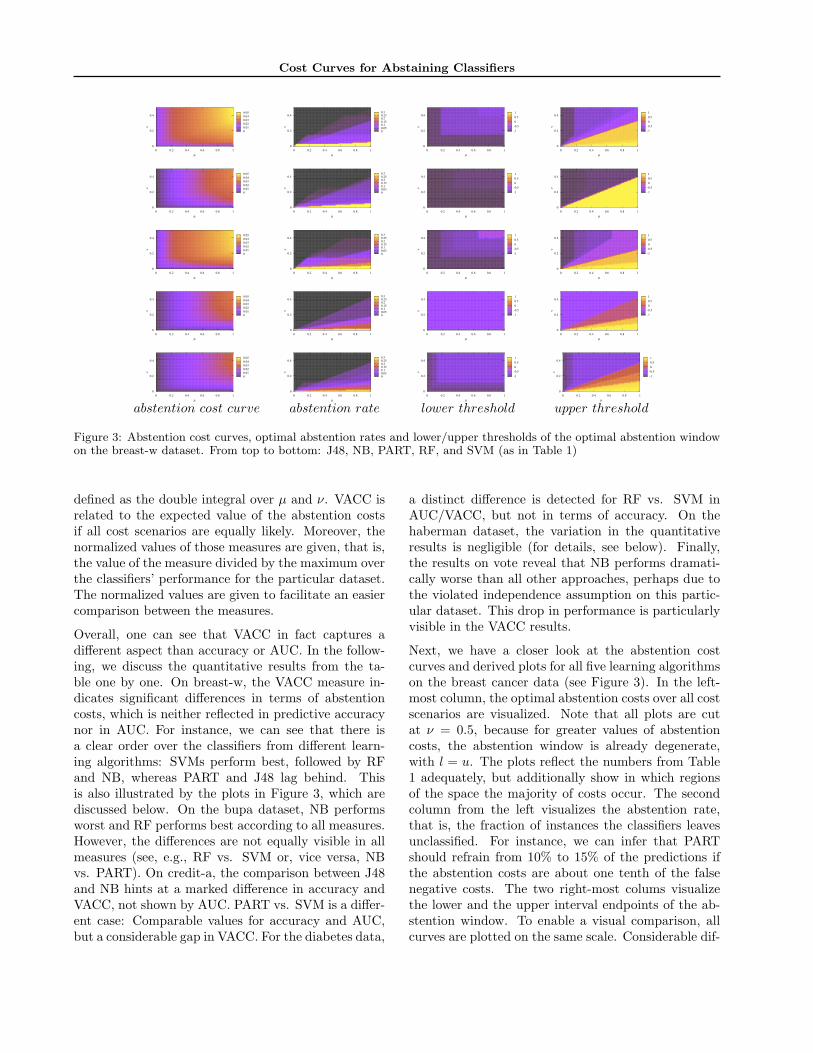
Figure 3: Abstention cost curves, optimal abstention rates and lower/upper thresholds of the optimal abstention windowon the breast-w dataset. From top to bottom: J48, NB, PART, RF, and SVM (as in Table 1)

defined as the double integral over µ and ν. VACC isrelated to the expected value of the abstention costsif all cost scenarios are equally likely. Moreover, thenormalized values of those measures are given, that is,the value of the measure divided by the maximum overthe classifiers’ performance for the particular dataset.The normalized values are given to facilitate an easiercomparison between the measures.

Overall, one can see that VACC in fact captures adifferent aspect than accuracy or AUC. In the follow-ing, we discuss the quantitative results from the ta-ble one by one. On breast-w, the VACC measure in-dicates significant differences in terms of abstentioncosts, which is neither reflected in predictive accuracynor in AUC. For instance, we can see that there isa clear order over the classifiers from different learn-ing algorithms: SVMs perform best, followed by RFand NB, whereas PART and J48 lag behind. Thisis also illustrated by the plots in Figure 3, which arediscussed below. On the bupa dataset, NB performsworst and RF performs best according to all measures.However, the differences are not equally visible in allmeasures (see, e.g., RF vs. SVM or, vice versa, NBvs. PART). On credit-a, the comparison between J48and NB hints at a marked difference in accuracy andVACC, not shown by AUC. PART vs. SVM is a differ-ent case: Comparable values for accuracy and AUC,but a considerable gap in VACC. For the diabetes data,

a distinct difference is detected for RF vs. SVM inAUC/VACC, but not in terms of accuracy. On thehaberman dataset, the variation in the quantitativeresults is negligible (for details, see below). Finally,the results on vote reveal that NB performs dramati-cally worse than all other approaches, perhaps due tothe violated independence assumption on this partic-ular dataset. This drop in performance is particularlyvisible in the VACC results.

Next, we have a closer look at the abstention costcurves and derived plots for all five learning algorithmson the breast cancer data (see Figure 3). In the left-most column, the optimal abstention costs over all costscenarios are visualized. Note that all plots are cutat ν = 0.5, because for greater values of abstentioncosts, the abstention window is already degenerate,with l = u. The plots reflect the numbers from Table1 adequately, but additionally show in which regionsof the space the majority of costs occur. The secondcolumn from the left visualizes the abstention rate,that is, the fraction of instances the classifiers leavesunclassified. For instance, we can infer that PARTshould refrain from 10% to 15% of the predictions ifthe abstention costs are about one tenth of the falsenegative costs. The two right-most colums visualizethe lower and the upper interval endpoints of the ab-stention window. To enable a visual comparison, allcurves are plotted on the same scale. Considerable dif-

Cost Curves for Abstaining Classifiers

-0.015-0.01-0.005 0 0.005 0.01 0.015 0.02 0.025 0.03

µ

ν

10.80.60.40.20

0.4

0.2

0

-0.01-0.005 0 0.005 0.01 0.015 0.02

µ

ν

10.80.60.40.20

0.4

0.2

0

-0.02-0.015-0.01-0.005 0 0.005 0.01

µ

ν

10.80.60.40.20

0.4

0.2

0

-0.02-0.015-0.01-0.005 0 0.005 0.01

µ

ν

10.80.60.40.20

0.4

0.2

0

J48 vs. PART (diabetes) J48 vs. PART (haberman) NB vs. PART (diabetes) NB vs. PART (haberman)(a) (b) (c) (d)

0 0.02 0.04 0.06 0.08 0.1 0.12 0.14

µ

ν

10.80.60.40.20

0.4

0.2

0

-1-0.5 0 0.5 1

µ

ν

10.80.60.40.20

0.4

0.2

0

-1-0.5 0 0.5 1

µ

ν

10.80.60.40.20

0.4

0.2

0

(e) (f) (g)Figure 4: Differential cost curves for large differences ((a) and (b)) and small differences in VACC ((c) and (d)), differentialcost curve SVMs vs. trivial classifier(s) on bupa (e), lower (f) and upper (g) thresholds of abstention window

ferences in the classifiers’ abstention behavior becomeapparent.

In the plots, the isolines of l and u have a remark-ably different shape. This can be explained as follows:First, both the upper and lower thresholds increasenot continuously with ν or µ, but in steps. This is dueto the fact that a critical value has to be reached forthe cost of abstaining or classifying the instances be-tween different threshold values, before thresholds areadjusted. Second, we observe that for values of ν forwhich abstaining is too expensive, the upper and thelower threshold are equal, as shown before.

The threshold shows a different behaviour only forthose values of ν and µ that allow abstaining. In thisrange, the lower threshold depends only on the ratiobetween false negative costs (which are constant) andabstaining costs, and is thus independent of the falsepositive costs. The upper threshold on the other handdepends on both the abstaining costs ν and the falsepositive costs µ. In the same way as the lower thresh-old is effectively not affected by changes in µ in therange for which abstaining is reasonable, the upperthreshold is not affected by changes in the false nega-tive costs, which can easily be confirmed by switchingthe positive and negative labels.

Next, we take a look at differential cost curves. Differ-ential cost curves are a tool for the practitioner to seein which regions of the cost space one classifier is tobe preferred over another. In Figure 4, differential costcurves with large differences in VACC (upper row, (a)and (b)) and small differences in VACC (upper row,(c) and (d)) are shown. In Figure 4(a) and (b), J48 de-cision trees have smaller abstention costs than PARTrules only in the bluish areas of the space. Differentialcost curves also shed light on differences that do notappear in VACC, if a classifier is dominating in oneregion as it is dominated in another (Figure 4 (c) and

(d)). The regions can be separated and quite distantin cost space, as illustrated by Figure 4 (c). The differ-ential cost curve of NB vs. PART on haberman (Fig-ure 4 (d)) demonstrates that even for datasets with noclear tendencies in accuracy, AUC or VACC, the plotover the cost space clearly identifies different regionsof preference not shown otherwise.

Another interesting possibility is the comparison withthe trivial classifier that always predicts positive, neg-ative, or always abstains. In Figure 4 (e), we compareSVMs with trivial classifiers on the bupa dataset. Inthe black areas near the left upper and the right lowercorner, the trivial classifer performs better than theSVM classifier. To explain this, we take a look at thelower and upper thresholds of the abstention windowin Figure 4 (f) and (g). Strikingly, we find that inthe upper left part l = u = −1, that is, everything isclassified as positive, because false positives are veryinexpensive compared to false negatives. However, inthe lower right part l = −1 and u = 1, i.e., not asingle prediction is made there, because abstention isinexpensive.

It is clear that the discussion of the above results re-mains largely on a descriptive level. However, ide-ally we would like to explain or even better, predictthe behavior of classifiers on particular datasets. Un-fortunately, this is hardly ever achieved in practice:In the majority of cases it is not possible to explainthe error rate or AUC for a particular machine learn-ing algorithm on a particular dataset at the currentstate of the art. To learn more about the behaviorof the abstention cost curve and the VACC measure,we performed preliminary experiments with J48 trees,varying the confidence level for pruning, and SVMs,varying the penalty/regularization parameter C. Overall datasets, we observed only small, gradual shifts inVACC and in the shape of the curves. While it ishard to detect a general pattern, it is clear that no

Cost Curves for Abstaining Classifiers

abrupt changes occur. It was also striking to see thatthe changes over varying parameter values were con-sistent for both learning schemes. It seems that theVACC depends, to some extent, on the noise level ofa dataset.

5. Related Work

The trade-off between coverage and accuracy has beenaddressed several times before, such as in articles by(Chow, 1970), who described an optimum rejectionrule based on the Bayes optimal classifier, or (Pazzaniet al., 1994), who showed that a number of machinelearning algorithms can be modified to increase accu-racy at the expense of abstention. Tortorella (Tor-torella, 2005) and Pietraszek (Pietraszek, 2005) useROC analysis to derive an optimal abstaining clas-sifier from binary classifiers. Pietraszek extends thecost-based framework of Tortorella, for which a simpleanalytical solution can be derived, and proposes twomodels in which either the abstention rate or the errorrate is bounded in order to deal with unknown absten-tion costs. Nevertheless, all of these ROC-based ap-proaches assume at least known misclassification costs.In contrast, abstention cost curves, as shown in thispaper, visualize optimal costs over a range of possi-ble cost matrices. Ferri and Hernandez-Orallo (Ferri& Hernandez-Orallo, 2004) introduce additional mea-sures of performance for, as they call it, cautious clas-sifiers, based on the confusion matrix. Our definitionof an abstention window can be considered as a spe-cial case of Ferri and Hernandez-Orallo’s model forthe two-class case. However, no optimization is per-formed when creating cautious classifiers and only thetrade-off between abstention rate and other perfor-mance measures such as accuracy is analyzed. Cau-tious classifiers can be combined in a nested cascadeto create so-called delegating classifiers (Ferri et al.,2004). Cost-sensitive active classifiers (Greiner et al.,2002) are related to abstaining classifiers as they areallowed to demand values of yet unspecified attributes,before committing themselves to a class label based oncosts of misclassifications and additional tests.

6. Conclusion

In this paper, we adopted a cost-based framework toanalyze and visualize classifier performance when re-fraining from prediction is allowed. We presented anovel type of cost curves that makes it possible tocompare classifiers as well as to determine the cost sce-narios which favor abstention if costs are uncertain orthe benefits of abstaining are unclear. In comprehen-sive experiments, we showed that adding abstention

as another dimension, the performance of classifiersvaries highly depending on datasets and costs. View-ing the optimal abstention behavior of various classi-fiers, we are entering largely unexplored territory. Weperformed preliminary experiments to shed some lighton the dependency of VACC on other quantities, suchas the noise level in a dataset. However, more workremains to be done to interpret the phenomena shownby the curves. Finally, we would like to note that an-other, more qualitative look at abstention is possible.In particular on structured data, refraining from clas-sification is advisable if the instance to be classified isnot like any other instance from the training set.

References

Chow, C. K. (1970). On optimum recognition error andreject tradeoff. IEEE Transactions on Information The-ory, 16, 41–46.

Drummond, C., & Holte, R. C. (2000). Explicitly repre-senting expected cost: An alternative to ROC represen-tation. Proc. of the 6th International Conf. on Knowl-edge Discovery and Data Mining (pp. 198–207).

Ferri, C., Flach, P., & Hernandez-Orallo, J. (2004). Dele-gating classifiers. Proc. of the 21st International Conf.on Machine Learning.

Ferri, C., & Hernandez-Orallo, J. (2004). Cautious clas-sifiers. Proceedings of the ROC Analysis in ArtificialIntelligence, 1st International Workshop (pp. 27–36).

Friedel, C. C. (2005). On abstaining classifiers. Mas-ter’s thesis, Ludwig-Maximilians-Universitat, Technis-che Universitat Munchen.

Greiner, R., Grove, A. J., & Roth, D. (2002). Learningcost-sensitive active classifiers. Artificial Intelligence,139, 137–174.

Pazzani, M. J., Murphy, P., Ali, K., & Schulenburg, D.(1994). Trading off coverage for accuracy in forecasts:Applications to clinical data analysis. Proceedings ofthe AAAI Symposium on AI in Medicine (pp. 106–110).Standford, CA.

Pietraszek, T. (2005). Optimizing abstaining classifiers us-ing ROC analysis. Proceedings of the 22nd InternationalConference on Machine Learning.

Provost, F. J., & Fawcett, T. (1998). Robust classificationsystems for imprecise environments. Proceedings of theFifteenth National Conference on Artificial Intelligence(pp. 706–713).

Tortorella, F. (2005). A ROC-based reject rule for di-chotomizers. Pattern Recognition Letters, 26, 167–180.

Witten, I., & Frank, E. (2005). Data mining: Practical ma-chine learning tools with java implementations. MorganKaufmann, San Francisco.