Cost-Benefit Analysis and the Marginal Cost ofPublic Funds

Nigar HashimzadeUniversity of Reading

Gareth D. Myles∗

University of Exeter and Institute for Fiscal Studies

21 December 2012

Abstract

The marginal cost of public funds (MCF ) measures the cost to theeconomy of raising government revenue. The MCF can be used to guidereform of the tax system and to determine an effi cient level of governmentexpenditure. It can also be used as an input into cost-benefit analysis.Previous applications of the concept have developed a methodology in acontext of a static economy. We extend the concept of the MCF to a set-ting that combines growth with infrastructural spill-overs across regions.

JEL Classification : E6, H4, H7Key Words : Growth, infrastructure, externalities, public funds

1 Introduction

All implementable government tax instruments are distortionary and, as a con-sequence, impose deadweight losses upon the economy. These distortions arethe inevitable cost of collecting the finance required to support public spending.The correct level of spending achieves a compromise between these distortionsand the benefits of spending. There are large literatures on cost-benefit analysis(Mishan and Quah, 2007) and optimal taxation (Myles, 1995) that describe howthis should be done. The purpose of this paper is to develop the methodology fordetermining when additional public spending is justified in a growing economywith externalities between regions.

∗Correspondence: Gareth Myles, Department of Economics, University of Exeter, Ex-eter, EX4 4PU, UK, gdmyles@ex.ac.uk.

Acknowledgement. Paper presented at the VIII Milan European Economy Workshop, June11-12, University of Milan, in the framework of the EIBURS project, sponsored by the Euro-pean Investment Bank. The authors are grateful for comments on an earlier draft to MassimoFlorio and participants of the Workshop. The usual disclaimer applies.

1

What matters for the spending decision is whether the marginal benefit ofspending exceeds the marginal cost of taxation. If it does, then additionalpublic spending is justified. This principle of contrasting marginal benefit andmarginal cost underlies the methodology of cost-benefit analysis. The survey ofDrèze and Stern (1987) provides a summary of the standard approach to cost-benefit analysis. That approach is based on the Arrow-Debreu representationof the competitive economy and its extensions. The generality of the modelpermits it to encompass many situations but for specific problems alternativemodels can be advantageous. The questions we wish to focus upon involveeconomic growth. Although growth can be handled by dating commodities inthe Arrow-Debreu framework it does seem preferable to employ a more specificmodel of the growth process. The model we analyze in this paper combinesendogenous growth and fiscal federalism. In addition, the government providesa productive input (which we view as infrastructure) that has spill-overs betweenjurisdictions.A government has access to a wide range of different tax instruments. Taxes

can be levied on consumption or on income. Different forms of consumption,and different sources of income, can be taxed at different rates. Taxes canalso be levied on firms, using profit, turnover, or input use as a base. Thecost of collecting revenue will depend upon the tax base that is chosen and thestructure of rates that are levied. The marginal cost of public funds (MCF ) is ameasure of the cost of raising tax revenue from a particular tax instrument. TheMCF can be used to identify changes to the tax structure that raise welfarekeeping expenditure constant. It can also identify the best tax instruments touse for raising additional revenue. It is a practical tool that permits consistentanalysis of taxation choices. Dahlby (2008) provides a detailed summary of theexisting methods for calculating the MCF in a wide variety of circumstancesand for a range of tax instruments. However, there is very little literature onthe derivation of the MCF for a growing economy.Section 2 of the paper provides a brief review of theMCF from a cost-benefit

perspective and a summary of several typical applications. Some of the issuesinvolved in applying theMCF to growing economies are discussed in Section 3.A general discussion of the MCF for a growing economy is given in Section 4.Section 5 analyses a basic model of endogenous growth and Section 6 extends themodel to incorporate infrastructural spill-overs and tax externalities. Section 7provides concluding comments.

2 Application of the MCF

The MCF provides a numerical summary of the cost of raising additional rev-enue from each tax instrument. The basic logic can be described as follows.Consider raising the income tax rate so that an extra €1 is collected from ataxpayer. Now offer the taxpayer the alternative of paying some amount di-rectly to the treasury in order to avoid the income tax increase. If the taxpayer

2

is willing to pay €1.20 then the MCF 1 is 1.2. Expressed alternatively, if theMCF is 1.2 an additional euro of government revenue imposes a cost of €1.20on the taxpayer.The MCF measures the welfare cost of raising revenue and so has a central

role in determining the range of projects that will be successful in a cost-benefitcalculation. There are two ways in which theMCF enters cost-benefit analysis.First, theMCF can be used to judge which projects should be adopted. Contin-uing the example above, a project that costs the government €1 and producesbenefits of €1.15 appears on the surface to be beneficial. However, if the MCFis €1.20 then the marginal benefit of the project falls short of the actual mar-ginal cost faced by the taxpayer. The project should therefore not be adopted.Second, the MCF can be employed to assess and improve the effi ciency of thetax system. If the tax structure is ineffi cient the MCF will be unnecessarilyhigh. This will reduce the range of projects that pass any given cost-benefitcriterion. The MCF can be used to guide the improvement of the effi ciency ofthe tax system and therefore increase the number of beneficial projects. In ourexample, if revision to the structure of income taxation reduced the MCF to€1.10 then the project with benefits of €1.15 should be accepted.A general construction of theMCF can be provided as follows. Consider an

economy that can employ m tax instruments to finance g public goods. Denotethe level of tax instrument i by τ i and the quantity of public good j by Gj .Welfare is given by the social welfare function W (τ ,G) where τ = (τ1, ..., τn)and G = (G1, ..., Gg) . The level of revenue by R (τ ,G) and the cost of the publicgood supply by C (G). Note that there is an interaction in the revenue functionbetween taxes and public good supply in revenue but the cost of public goodsis determined by technology alone.The optimization problem for the government is2

max{τ,G}

W (τ ,G) s.t. R (τ ,G) ≥ C (G) . (1)

To analyze the solution to this optimization define λi by

λi = −∂W/∂τ i∂R/∂τ i

, i = 1, ...,m. (2)

The term λi is the Marginal Cost of Funds from tax instrument i (MCFi). Itmeasures the cost, in units of welfare, of raising an additional unit of revenue.3

If the tax system is effi cient then the MCFi is equalized across the differenttax instruments: λi = λ, for all i. (The converse does not necessarily hold:the common value can be negative, implying that the level of revenue is fallingas taxes increase, or even zero. Neither situation is effi cient.) If the value of

1Formally, it is the “normalized MCF” defined later in the paper that is described here.The MCF is denominated in units of welfare per dollar whereas the normalized MCF isunit-free.

2The solution to this optimization is studied in detail in Atkinson and Stern (1974) .3 In applications revenue is typically denominated in monetary units but in this formal

(non-monetary) model it is denominated in units of the numeraire commodity.

3

λi differs across tax instruments then welfare can be raised by collecting morerevenue from taxes with low (but positive) λi and less revenue from those withhigh λi.Now assume that the tax instruments have been optimized so that MCFi =

MCF > 0 for all i (that is, λi = λ > 0). The use of the MCF in project choicecan be illustrated by writing the optimality condition for the level of publicgood j as

∂W

∂Gj= λ

[∂C

∂Gj− ∂R

∂Gj

], j = 1, ..., g. (3)

This conditions says that the quantity of provision of each public good is optimalwhen the marginal benefit of that extra provision (∂W/∂Gj) is equal to the netcost of the public good (∂C/∂Gj − ∂R/∂Gj) converted into welfare units usingthe MCF .The properties of the MCFi and the MCF are investigated in Hashimzade

and Myles (2012). The paper assumes that ∂W/∂τ i is negative for low τ i butmay become zero for high τ i (if the tax is suffi ciently high to discourage therespective activity), and that ∂R/∂τ i is positive for low τ i (the “upward”slopeof the Laffer curve), possibly negative for higher τ i, and, eventually, may becomezero. Under these assumptions it is shown that λi can, in principle, take anyvalue, including ±∞, or can be undefined (when both ∂W/∂τ i and ∂R/∂τ i arezero). It is also has a discontinuity at the value of τ i that maximizes revenue(given the value of other tax instruments).The definition in (2) shows that the MCFi and the MCF are denominated

in units of welfare/revenue and that can be used to convert monetary costs intowelfare equivalents. Furthermore, the MCFi and the MCF are unique only upto multiplicative transformation, both in the cases when W (τ ,G) is ordinal orcardinal. That is, given n tax instruments, for every permissible transformationof the social welfare function there is a choice of n different numeraires forrevenue and each results in a different numerical value for λi and λ. Anotherway to look at this is that λi is denominated in units of welfare/revenue, andits value changes when we change the units of measurement for either welfare orrevenue. One response to this fact is to accept that the MCFi provides only aranking of tax instruments (and theMCF a ranking of the effi cient tax systems)for a given transformation of the welfare function and choice of numeraire. Inother words, the ranking is ordinal, and so the numerical value is not in itselfmeaningful. An alternative response is to develop a unit-free form of the MCFi(and the MCF ) that is not affected by transformation of the social welfarefunction or choice of numeraire.To produce a unit-free version of the MCFi let ν be any quantity measured

in welfare/revenue units. Then a normalized form of the MCFi is given by

λNi =λiν. (4)

For given ν the value of λNi is uniquely defined since any transformation of thewelfare function or change in numeraire must be applied to ν as well as λi.

4

However, this does not make the measure unique since the tax rates and publicgood levels at which the normalizing factor, ν, is evaluated need to be chosen.Different choices will provide different numerical values of λNi . This point canbe seen by considering a model with a representative consumer. In that caseone can use the private marginal utility of income4 , henceforth denoted α (τ ,G),as the normalizing factor. The value of the marginal utility will depend upon

of τ and G at which it is evaluated. The choose of specific values,{τ , G

}, is

constrained by the requirement at R(τ , G

)≥ C

(G); each choice satisfying

this condition is equally acceptable but will result in a different numerical valuefor λNi .Hashimzade and Myles (2012) also observe that a unit-free MCFi can be

obtained by using the compensating variation or equivalent variation to mea-sure welfare change (see also Diamond and McFadden, 1974). The use of such“money-metric” welfare measures solves one set of issues but raises another:the aggregation of the money-metric measure across heterogeneous consumers.This is an issue for which there is no compelling resolution (Hammond, 1994).We would like to emphasize that using the comparison of the numerical

values for theMCFi obtained under different normalization and different welfaremeasures is inappropriate. Furthermore, using the extent to which the MCFifor a particular tax instrument differs from 1 as the measure of the degree ofdistortion of that instrument can be misleading. This is an important pointsince many applications implicitly assume that an MCFi of 1 represents a non-distortionary tax instrument and that any distortionary tax must have anMCFiin excess of 1. In fact, as shown in Atkinson and Stern (1974), the MCFicalculated using normalisation by the private marginal utility of income can beless than 1 for a distortionary tax system (labour income tax) if the incomeeffect on labor supply is suffi ciently negative.This non-uniqueness in the definition of theMCF is linked to the discussion

of the use of the differential approach versus the balanced-budget approach tothe analysis of the welfare cost of taxation (Ballard, 1990). Differential analysiscompares alternative means of raising the same amount of revenue, whereas thebalanced-budget analysis is concerned with a change in the level of revenue anda simultaneous change of the tax system to finance this additional revenue. Thenumerical value can be very sensitive to the choice of the welfare measure andthe reference point, as shown in Triest (1990). While a chosen normalization canbe used to compare the extent of welfare loss under two different distortionarytax instruments, it cannot be meaningfully used to measure the extent of welfareloss under one particular distortionary tax system.There is substantial literature on the application of the MCF showing how

it can be used to optimize the tax structure and to determine whether a pub-lic project is welfare-enhancing (Slemrod and Yitzhaki, 2001), or to comparethe degree of distortion of various tax instruments. For example, Parry (2003)

4The private marginal utility of income is defined as the derivative of the indirect utilityfunction with respect to income.

5

considers the excise taxes on petroleum, alcoholic drinks, and cigarettes in theUK. It is shown that petroleum taxes are the most distortionary of the instru-ments and the cigarette taxes are the least distortionary. These calculationsdemonstrate that the current system is only optimal if the goods have externaleffects or differ in the degree of tax shifting. The role of tax shifting is exploredin Delipalla and O’Donnell (2001). Many applications of the MCF are under-taken for linear tax structures but Dahlby (1998) shows how the MCF can beextended to accommodate a progressive income tax. The approach of Dahlbyis applied in a study of the Japanese income tax system by Bessho and Hayahi(2005). A alternative extension is made by Kleven and Kreiner (2006) who showhow labour force participation can be included in a measure of theMCF . Theycalculate theMCF for five European countries and show that incorporating theparticipation margin can significantly increase theMCF in some circumstances.Poapangsakorn et al. (2000) employ the MCF in a cost-benefit analysis of atax enforcement programme in Thailand and conclude that the tax enforcementprogramme was a high-cost method of raising revenue. Elmendorf and Mankiw(1999) analyze the MCF of public sector debt when interest payments on debtare financed by a distortionary tax on total output. Debt finance can smooththe MCF over time when a lumpy project is financed. This can lead to asignificant welfare gain.This section has shown how theMCF developed in the formal literature into

a set of techniques that permit the MCF to be calculated and to be integratedinto cost-benefit analysis. Numerous further examples of such applications aredescribed in the comprehensive text of Dahlby (2008). However, despite thisextensive literature there are still a number of significant issues that need to beaddressed if the MCF is to be used effectively in policy design.

3 The MCF and Economic Growth

The analysis of the MCF given above is very general and, conceptually, canbe applied to any economy. The cost of this generality is an absence of de-tail concerning the economic model behind the welfare function and the costfunction. This observation becomes important when the MCF is applied topractical policy questions. For example, applying the MCF to the case of aneconomy with multiple jurisdiction or an economic union, such as the EU, raisesseveral questions. First, the use of a single objective function is an issue in anintegrated economic area but with subsidiarity permitting independence in pol-icy. Secondly, the economic integration amplifies externalities between memberstates of the EU or between jurisdictions in a federal state, that are not capturedby the general formulation. Finally, the relationship between fiscal policy andeconomic growth has emerged in recent years as a focal point for the attentionof EU policy makers. In contrast, almost all analysis of the MCF has beenundertaken for static economies.The implication of these comments is that there are benefits to be obtained

by refining the analysis of the MCF to apply in a growth model with mul-

6

tiple jurisdictions. The formal developments of the MCF have been basedupon the Arrow-Debreu model which can incorporate time in the form of datedcommodities but must have all contracts agreed prior to the commencement ofeconomic activity. Consequently, it is not a compelling representation of thegrowth process. Similarly, the applications of the MCF reviewed are typicallyset within a single-country model. Such a refinement would need to includethe role of individual member states and the externalities that link the memberstates. Dahlby and Wilson (2003) make some progress in this respect by ana-lyzing a model that includes fiscal externalities. Their model has both a centralgovernment and a local government. Both governments levy taxes on labour in-comes and profit so there are vertical tax externalities linking the two levels ofgovernment. The main result is the demonstration that a local government thatdoes not take into account the effect of its choices on the central governmentmay have an MCF that is biased up or down.Endogenous growth occurs when capital and labour are augmented by addi-

tional inputs in a production function that otherwise has non-increasing returnsto scale. One interesting case for understanding the link between governmentpolicy and growth is when the additional input is a public good or public in-frastructure financed by taxation. The need for public infrastructure to supportprivate capital in production provides a positive role for public expenditure anda direct mechanism through which policy can affect growth. Introducing in-frastructure permits an analysis of the optimal level of public expenditure in anendogenous growth model.The importance of infrastructure is widely recognized, not least by the EU

which pursues an active programme to support the investment activities of mem-ber states. The policy problem facing the EU is to ensure that member statesundertake an effi cient level of infrastructural expenditure that ensures the max-imum rate of growth. The determination of the level has to take into accountthe full consequences of an infrastructure project for the EU, not just the di-rect benefits for the member state undertaking the investment. The MCF canbe used to evaluate public infrastructure provision but its use has to recognizethree significant issues. First, infrastructural investment has significant spill-overs across member states. Second, mobility of the tax base results in taxexternalities between the member states, and between the member states andthe EU. Third, the EU is faced with a decision on how to allocate support forinfrastructural expenditure across the different member states. This interactswith the process of revenue-raising, and with the extent to which the projectsare financed jointly by the EU and member states. The same is true of therelationship between the local and central government financing in a federalstate.The economic modelling of the impact of infrastructure on economic growth

has focussed on the Barro (1990) model of public expenditure as a public inputand its extensions (Chen et al. 2005, Turnovsky, 1999). This literature hasidentified the concept of an optimal level of expenditure, and has highlightedthe deleterious effects of both inadequate and excessive expenditure. These areimportant insights, but they do not address the spill-over issues that confront a

7

federation. Infrastructural spill-overs between the members of a federation canbe positive, which occurs when improvements in infrastructure in one regionraise productivity in another, or they can be negative if they induce relocation ofcapital between regions. In either case, it is important that the consequences ofspill-overs are addressed in order for the role of productive public expenditure tobe fully understood. Ignoring either form of spill-over will result in an ineffi cientlevel and allocation of expenditure.The EU single-market programme has increased the degree of capital mobil-

ity. The flow of capital provides an important mechanism for equalizing growthrates. An economy with a high rate of growth will pay a high return to capital.This will attract an inflow of mobile capital and a consequent reduction in thereturn. It will also increase the level of GDP but decrease the growth rate. Theconverse in true for countries experiencing capital outflows. Hence, mobility ofcapital will equalize the growth rate across countries and increased mobility willreduce the time taken for this process to operate. The observation that capitalflows reduce growth differentials between countries has been made previously byRazin and Yuen (1997). They argued that labour mobility equalized incomesacross countries when there were human capital externalities. Similar issueshave also been addressed by Bianconi and Turnovsky (1997), but in a modelthat does not have public infrastructure. The effect of these capital flows is tomake government policy even more important than in a world without spill-overs since additional public infrastructure in one country can raise the growthrate in all. This gives further emphasis to the development of an appropriateconcept of the MCF .

4 Dynamic Setting

There has been little investigation of the MCF in growing economies. Twoexceptions are Liu (2003) who computes the MCF as a component of a cost-benefit analysis (but taking the intertemporal path of wage rates and interestrates as exogenous) and Dahlby (2006) who uses the MCF to analyze publicdebt in an AK growth model. Our approach is similar to Dahlby but we employa more general model of endogenous growth. In principle, it is possible to treatthe economy lying behind (1) as intertemporal but the analysis needs to be morespecific to generate worthwhile conclusions.Consider an intertemporal economy set in discrete time. The time path for

tax instrument i is a sequence{τ1i , τ

2i , . . .

}. The MCF is computed for a vari-

ation in this sequence. A pulse variation takes the form of a change in thetax instrument in a single time period, t. The new sequence would then be{τ1i , . . . , τ

t−1i , τ ti, τ

t+1i , . . .

}. Alternatively, a sustained variation in the tax in-

strument from period t onwards changes the sequence to{τ1i , . . . , τ

t−1i , τ ti, τ

t+1i , . . .

}.

We choose to focus on sustained variations. Correspondingly, we extend the de-

8

finition of theMCF for a static economy to an intertemporal economy by using

MCF ti ≡ −∂W/∂τ i∂R/∂τ i

,

to denote the MCF of a sustained variation in tax instrument i from period tonwards. In this setting W is the intertemporal social welfare function, and Ris discounted value of tax revenue.In a dynamic, infinite horizon economy

R =

∞∑t=0

d (t)Rt,

where Rt is tax revenue in period t, and d (t) is the discount factor applied torevenues in period t. There are many well-known issues involved in the choice ofthe sequence of discount factors {d (t)}. We choose to remain with the standardconvention (see, for example, Nordhaus 2008) of appealing to market equilibriumto determine the social rate of time preference endogenously. In this case

d (t) =∂W/∂Ct∂W/∂C0

,

where Ct is consumption at time t. If the welfare function is time-separablewith exponential discounting, that is, W =

∑∞t=0 β

tU (Ct), then

d (t) = βtU ′ (Ct+1)

U ′ (C0). (5)

The purpose of the analysis is to apply theMCF in settings where economicgrowth is occurring. This requires us to embed the MCF within a model ofendogenous growth. The major diffi cultly involved in achieving this is that,generally, the entire intertemporal path for the economy must be computedfrom the present into the indefinite future. To overcome this diffi culty we focusupon balanced growth paths. Along a balanced growth path all real variablesgrow at the same rate, so such a path can be interpreted as describing thepattern of long-run growth. All the commonly used growth models have theproperty that the economy will converge to a balanced growth path from anarbitrary initial position.

5 Public Infrastructure

This section develops the MCF for a growing economy by building on theBarro (1990) model of productive public expenditure. In particular, the modelis used to illustrate the benefits of focussing on the balanced growth path. Thisanalysis provides the developments that we need to combine endogenous growthwith fiscal federalism and infrastructural spill-overs in Section 6.

9

Public infrastructure is introduced by assuming that the production functionfor the representative firm at time t has the form

Yt = AL1−αt Kαt G

1−αt ,

where A is a positive constant and Gt is the quantity of public infrastructure.The form of this production function ensures that there are constant returns toscale in labour, Lt, and private capital, Kt, for the firm given a fixed level ofpublic infrastructure. Although returns are decreasing to private capital as thelevel of capital is increased for fixed levels of labour and public input, there areconstant returns to scale in public input and private capital together.

5.1 Output Tax

The first step is to consider the MCF when the productive public input isfinanced by a tax upon output as in Barro (1990). Let τ denote the tax uponoutput. The firm belongs to a representative infinitely-lived household whosepreferences are described by an instantaneous utility function, U = ln (Ct).The household maximizes the infinite discounted stream of utility, subject tothe sequence of intertemporal budget constraints, and with the sequence oftaxes and government infrastructure taken as given. The public capital inputis financed by the tax on output, and there is no government debt, so that thegovernment budget constraint is

Gt = τYt.

This constraint assumes that public capital fully depreciates in one period; inother words, it is a flow variable, rather than a stock variable. We relax thisassumption in the later analysis.On a balanced growth path the real variables (Yt, Ct,Kt, Gt) grow at the

same constant rate, γ. Markets also clear in every period and the interest rateis constant.We assume for this analysis that labour supply is constant, andnormalize it to one. Along the balanced growth path Ct+1 = (1 + γ)Ct whereγ is the rate of growth.Following Dahlby (2006) we define theMCFN (the “normalizedMCF”) by

dividing the MCF in by the marginal utility of income at time 0,

MCFN = − 1

∂W/∂I0

∂W/∂τ

∂R/∂τ(6)

This provides a unit-free measure of the cost of public funds. For the specifica-tion of utility in this model the marginal utility of income at time 0 is given by1/C0 = 1/cK0. Hence,5

MCFN = 1− αβ +αβ2

1− βc

1 + γ. (7)

5See Appendix for details.

10

0 0.25 0.5 0.75­0.4

­0.2

0

0.2

τ

Growth Rate

γ

0 0.25 0.5 0.751

1.25

1.5

1.75

τ

MCFN

λ

0 0.25 0.5 0.75

­10

­5

0

5

τ

Welfare

W

0 0.25 0.5 0.750

0.25

0.5

0.75

τ

c

Consumption Capital Ratio

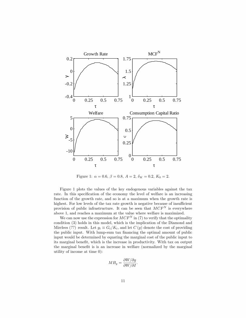
Figure 1: α = 0.6, β = 0.8, A = 2, δK = 0.2, K0 = 2.

Figure 1 plots the values of the key endogenous variables against the taxrate. In this specification of the economy the level of welfare is an increasingfunction of the growth rate, and so is at a maximum when the growth rate ishighest. For low levels of the tax rate growth is negative because of insuffi cientprovision of public infrastructure. It can be seen that MCFN is everywhereabove 1, and reaches a maximum at the value where welfare is maximized.

We can now use the expression forMCFN in (7) to verify that the optimalitycondition (3) holds in this model, which is the implication of the Diamond andMirrlees (??) result. Let gt ≡ Gt/Kt, and let C (g) denote the cost of providingthe public input. With lump-sum tax financing the optimal amount of publicinput would be determined by equating the marginal cost of the public input toits marginal benefit, which is the increase in productivity. With tax on outputthe marginal benefit is is an increase in welfare (normalized by the marginalutility of income at time 0):

MBg =∂W/∂g

∂W/∂I.

11

The optimality condition requires

MBg = MCFN(∂C

∂g− ∂R

∂g

),

or∂C

∂g=∂R

∂g+

MBgMCFN

=1− α1− βAK0g

−α,

which is exactly the same as (30) for the lump-sum tax financing of the publicinput, i.e. the Diamond and Mirrlees (1971) result that optimal tax systemdoes not distort production decision holds in this situation. (See Appendix fordetails.)

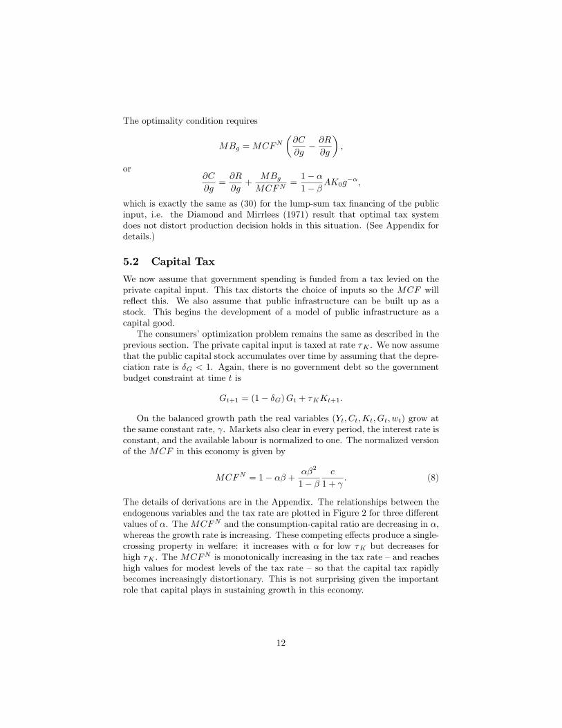
5.2 Capital Tax

We now assume that government spending is funded from a tax levied on theprivate capital input. This tax distorts the choice of inputs so the MCF willreflect this. We also assume that public infrastructure can be built up as astock. This begins the development of a model of public infrastructure as acapital good.The consumers’optimization problem remains the same as described in the

previous section. The private capital input is taxed at rate τK . We now assumethat the public capital stock accumulates over time by assuming that the depre-ciation rate is δG < 1. Again, there is no government debt so the governmentbudget constraint at time t is

Gt+1 = (1− δG)Gt + τKKt+1.

On the balanced growth path the real variables (Yt, Ct,Kt, Gt, wt) grow atthe same constant rate, γ. Markets also clear in every period, the interest rate isconstant, and the available labour is normalized to one. The normalized versionof the MCF in this economy is given by

MCFN = 1− αβ +αβ2

1− βc

1 + γ. (8)

The details of derivations are in the Appendix. The relationships between theendogenous variables and the tax rate are plotted in Figure 2 for three differentvalues of α. TheMCFN and the consumption-capital ratio are decreasing in α,whereas the growth rate is increasing. These competing effects produce a single-crossing property in welfare: it increases with α for low τK but decreases forhigh τK . The MCFN is monotonically increasing in the tax rate —and reacheshigh values for modest levels of the tax rate —so that the capital tax rapidlybecomes increasingly distortionary. This is not surprising given the importantrole that capital plays in sustaining growth in this economy.

12

0 0.2 0.4­0.1

0

0.1

τK

γ

Growth Rate

0 0.2 0.41.2

1.5

1.8

2.1

τK

λ

MCFN

0 0.2 0.4­4

­2

0

2

4

τK

W

Welfare

0 0.2 0.40.3

0.6

0.9

τK

c

Consumption Capital Ratio

Figure 2: α = 0.6 (solid), 0.65 (dash), 0.7 (dot), β = 0.8, δK = δG = 0.15,A = 1, K0 = 2.

13

5.3 Tax on capital and labour

The model is now extended to make labour supply elastic. This is achieved bymodifying the utility function to include labour as an argument. This makes itinteresting to analyze a capital tax and a labour tax since both instruments aredistortionary.We now assume that the instantaneous utility has the Cobb-Douglas form

U (Ct, 1− Lt) = θ ln (Ct) + (1− θ) ln (1− Lt) . (9)

Labour income is taxed at rate τL, and the private capital input is taxed at rateτK . The public capital input is financed by the tax on capital input and on thelabour income. We assume, as before, that the government does not issue debt.The government budget constraint in period t is therefore

Gt = (1− δG)Gt−1 + τKKt + τLwtLt.

The achievement of the balanced growth path when public capital is modelledas a stock variable has been analyzed in Gómez (2004) and Turnovsky (1997).Turnovsky assumes that investments in public capital and private capital arereversible. This allows immediate adjustment to the balanced growth path viaa downward jump in one of the capital stock variables. Without reversibility itis shown by Gómez that the optimal transition path requires investment in oneof the two capital variables to be zero until the balanced growth path is reached.The normalized MCF s for the two instruments are6

MCFNK =c

τK

[εKc − (1− τL)

ω

cεKL +

β

1− βγ

1 + γεKγ

],

MCFNL =c

ωτL (1 + εLω)

[εLc − (1− τL)

ω

cεLL +

β

1− βγ

1 + γεLγ

],

where

εic ≡τ ic

∂c

∂τ i, εiL ≡

τ iL

∂L

∂τ i, εiγ ≡

τ iγ

∂γ

∂τ i, i = K,L.

are elasticites with respect to the tax rates.The expressions we have derived for two tax instruments are now numerically

analyzed for a calibrated version of the model. For the model’s parameters weemploy values that are broadly consistent with the calibration of business cycleand growth models; see, for example, Cooley and Prescott (1995). The firststep is to evaluate the elasticities that appear in the MCF formulae to providean insight into the relative magnitude of effects in the model. The second stepis to present an evaluation of the MCF .It should be noted that these are not behavioral elasticities but are instead

the elasticities of equilibrium values. The elasticities are also not constant butdepend on the tax rates at which they are evaluated. The results reported inTable 1 show that the elasticity of the equilibrium consumption-capital ratio, c,

6See Appendix for details.

14

and the elasticity of the equilibrium quantity of labour have the expected signsbut are small in value. The elasticity of the growth rate (which reflects changesin capital accumulation) is negative and large for both taxes.

εKc εKL εKγ-0.0225 0.0347 -15.91εLc εLL εLγ

-0.3878 -0.0629 -1.648Table 1: Elasticities (τK = τL = 0.25)

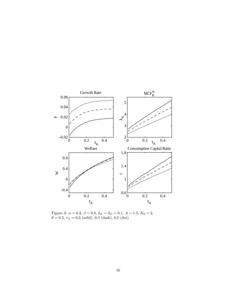
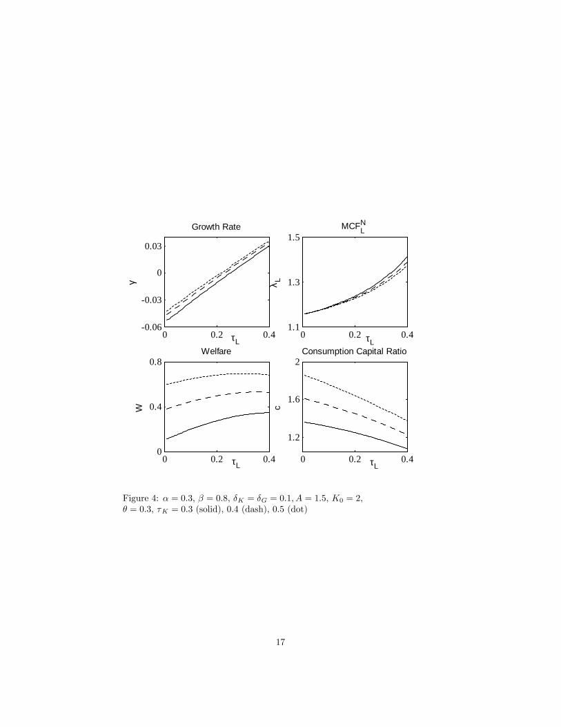
Figure 3 shows how the growth rate, level of welfare, consumption-capitalratio, and MCFNK for the capital tax change with the rate of tax on privatecapital input, for three different levels of labour income tax. In Figure 4 theroles of the capital tax and the labour tax are reversed and theMCFNL is plottedfor three values of the tax on labour income. These figures show that there isno longer a direct link between the growth rate and the level of welfare. In fact,the maximum rate of growth is achieved before welfare is maximized. Over therange plotted in Figure 3 one can see that the decrease in consumption witha higher rate of labour income tax in this economy is more than offset by theincrease in the growth rate, so that for a given level of the capital tax the welfarelevel is higher with a higher labour tax rate. A similar pattern is observed forthe capital tax. MCFNK is reduced by an increase in labour tax but, conversely,MCFNL is raised by an increase in capital tax. Both MCFNK and MCFNLincrease rapidly as the tax rates are raised and MCFNL is clearly convex in thetax rate. Both are less than one for low tax rates since the growth-enhancingeffect is dominant and exceed two for moderate values of the tax rates. The factthat theMCFNK is greater than theMCFNL is a reflection of the Chamley-Juddresult that the optimal capital tax in a growth model should be zero (Chamley1986, Judd 1985).

6 Infrastructural Spill-Overs

This section analyzes a model that incorporates infrastructural spill-overs be-tween regions. The discussion that follows refers to the EU context; the sameanalysis applies to a federal state with multiple jurisdictions.The model is designed to capture the important feature of the EU that

productive investments by one member state have benefits for other neighboringstates. In general, independent policy-setting by countries will lead to under-investment in infrastructure in such a setting because of the positive externalitygenerated by the spill-over. This provides a role for a supra-national body tocoordinate the decisions of individual countries so as to secure an increase inthe growth rate. It also has implications for the value of the MCF .We first introduce externalities in productive public input between two coun-

tries. Let Gt and G∗t denote productive public input in the home and in theforeign country, respectively, and let Γt = Gt +G∗t be the total public input athome and abroad. The level of output in the home country is given by

15

0 0.2 0.4­0.02

0

0.02

0.04

0.06

τK

γ

Growth Rate

0 0.2 0.42

3

4

5

τK

λ K

MCFNK

0 0.2 0.4­0.4

0

0.4

0.8

τK

W

Welfare

0 0.2 0.40.6

1

1.4

1.8

τK

c

Consumption Capital Ratio

Figure 3: α = 0.3, β = 0.8, δK = δG = 0.1, A = 1.5, K0 = 2,θ = 0.3, τL = 0.3 (solid), 0.4 (dash), 0.5 (dot)

16

0 0.2 0.4­0.06

­0.03

0

0.03

τL

γ

Growth Rate

0 0.2 0.41.1

1.3

1.5

τL

λ L

MCFLN

0 0.2 0.40

0.4

0.8

τL

W

Welfare

0 0.2 0.4

1.2

1.6

2

τL

c

Consumption Capital Ratio

Figure 4: α = 0.3, β = 0.8, δK = δG = 0.1, A = 1.5, K0 = 2,θ = 0.3, τK = 0.3 (solid), 0.4 (dash), 0.5 (dot)

17

Yt = AL1−αt Kαt

(G1−ρt Γρt

)1−α. (10)

There is no externality when ρ = 0. To simplify the analysis we assume labouris inelastic and normalize the quantity to one. The optimization problem of thehome consumer is to maximize intertemporal utility taking as given the levelsof capital and public good as well as the rate of growth in the foreign country.For now we assume there is no redistribution of the tax revenues across

countries, and that the home and the foreign countries set their tax rates inde-pendently. The home (foreign) country finances their public spending by taxingthe private capital input at rate τK (τ∗K), and there is no government debt.Thus, for the home country

Gt = (1− δG)Gt−1 + τKKt. (11)

We focus on balanced growth paths along which all real variables in allcountries grow at the same rate and the tax rates are constant over time. Theequality of the growth rates across countries here is imposed, since the law ofmotion of the public capital in one country only ensures that the growth ratesof the stock of public and private capital are equal in that country, but there isno reason of why the growth rates should be equal across countries. If we didnot impose this assumption then the output of one country would eventuallybecome arbitrarily small relative to the output of the other.When the externality from the infrastructural spill-over is present, W de-

pends on the growth rate in both home and foreign country. Thus, in the pres-ence of externalities, the welfare of the home consumer depends on the hometax rate through its own growth rate as well as the growth rate in the foreigncountry

∂W

∂τK=

∂W

∂τK

∣∣∣∣γ,γ∗

+∂W

∂γ

∂γ

∂τK+∂W

∂γ∗∂γ∗

∂τK. (12)

The details of the calculations are provided in the Appendix and in Hashimzadeand Myles (2010).The MCFN is given by

MCFN = (1− β) c

[∂W

∂τK

∣∣∣∣γ,γ∗

+∂W

∂γ

∂γ

∂τK+∂W

∂γ∗∂γ∗

∂τK

]γ=γ∗

. (13)

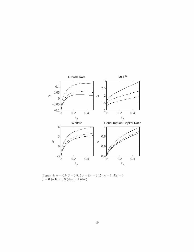
Figure 5 depicts the solution for symmetric equilibrium in the model withtwo identical countries. It can be seen that an increase in the extent of the spill-over (measured by ρ) reduces MCFN , so that greater spill-overs decrease thecost of funding projects. One explanation for an increased spill-over could beeconomic integration, which suggests that the single-market programme mayhave consequences for the cost of financing public projects. The MCFN in-creases with the tax rate but over the range displayed so do the growth rate andwelfare.

18

0 0.2 0.4­0.1

­0.05

0

0.05

0.1

τK

γ

Growth Rate

0 0.2 0.41

1.5

2

2.5

3

τK

λ

MCFN

0 0.2 0.4­3

0

3

6

τK

W

Welfare

0 0.2 0.40.4

0.6

0.8

1

τK

c

Consumption Capital Ratio

Figure 5: α = 0.6 β = 0.8, δK = δG = 0.15, A = 1, K0 = 2,ρ = 0 (solid), 0.3 (dash), 1 (dot).

19

7 Conclusions

The marginal cost of public funds has a central role in the assessment of taxpolicy and in cost-benefit analysis. The MCF provides a measure of the costof raising revenue through distortionary taxation that can be set against thebenefits of a public sector project. Despite the importance of the concept thecurrent literature has focussed upon the MCF in static settings. Only a verysmall literature has so far considered it within a growth setting.In this paper we have computed theMCF in a variety of endogenous growth

models with public infrastructure. To do this we have built upon the definitionof theMCF in an intertemporal setting provided by Dahlby (2006). The modelsthat have been analyzed are extensions of the Barro model of productive publicexpenditure, but with the public input represented as a stock rather than a flow.In addition, we have also introduced externalities between countries which area consequence of spill-overs from public infrastructure. To evaluate the MCFwe assume that the economy is on a balanced growth path which permits theevaluation of welfare in terms of a balanced growth rate. This technique providesa basis for determining theMCF for a variety of tax instruments in a form thatcan be empirically evaluated.We have employed the standard parameter values for calibration used in real

business cycle and growth models to simulate the models. Our results demon-strate that there is a link between the MCF and the growth rate, and that theMCF is sensitive to the tax rate. In the calibrated simulation the normalizedMCF can take high values for quite reasonable values of tax rates. This indi-cates that the effect upon the growth rate can exacerbate the static distortionscaused by taxation. In every case the MCF is increasing and monotonic overa range of capital and income tax rates similar to those seen in practice. Inthe model with an infrastructural spill-over it is interesting to observe that anincrease in the spill-over effect reduced the MCF .

The analysis has been restricted here by the focus on balanced growth paths.It might be thought necessary to consider the transition path but there is limitedevidence on the length of such transition. We have considered only sustainedvariations in tax rates and have implicitly assumed credibility of governmentannouncements and commitment to announced policies. This removed any needto consider the formation of expectations or games played between the publicand private sectors. If there is any strategic interaction this would change thevalue of the MCF .7 The benefit of these restrictions is the simplification theyprovide to the analysis and the fact that they can be applied in a similar mannerto more complex models.The MCF is an important concept in tax policy and cost-benefit analysis.

Although it generally appears in a static setting it can be extended to growth

7An example can illustrate the potential effects of game-playing. A tax on the profit fromdeveloping land has been introduced twice in the past 100 years in the UK. On both occasionsdevelopers held back from undertaking development in the belief that the next governmentwould repeal the tax. This belief was proved correct. Hence, a significant short-term welfarecost was incurred for the generation of very little revenue.

20

models. Our approach to the MCF is suitable for numerical evaluation in morecomplex economic environments. An avenue for exploring the practical value ofthis methodology could be to consider the effect of capital mobility upon theMCF , and to embed it in a more general model that can incorporate severalcountries and a broader range of tax instruments. This latter model will formthe basis of empirical implementation using a combination of calibration andestimation.

References

Atkinson, A.B. and N.H. Stern (1974) “Pigou, taxation and public goods”,Review of Economic Studies, 41, 119 —128.

Ballard, C. L. (1990) “Marginal welfare cost calculations: Differential analysisvs. balanced-budget analysis,” Journal of Public Economics, 41, 263 —276.

Barro, R.J. (1990) “Government spending in a simple model of endogenousgrowth”, Journal of Political Economy, 98, S103 —S125.

Bessho, S. and Hayahi, M. (2005) “The social cost of public funds: the case ofJapanese progressive income taxation”, Ministry of Finance, Japan, PolicyResearch Institute Paper 05A-16.

Chamley, C. 1986. Optimal taxation of capital income in general equilibriumwith infinite lives. Econometrica 54: 607—22.

Cooley, T.F. and E.C. Prescott (1995). Economic growth and business cycles,in: Cooley, T.F. (Ed.) Frontiers of business cycle research. Princeton:Princeton University Press.

Dahlby, B. (1998) “Progressive taxation and the social marginal cost of publicfunds”, Journal of Public Economics, 67, 105 —12.

Dahlby, B. (2006) “The marginal cost of funds from public sector borrowing”,Topics in Economic Analysis and Policy, 6, 1 —28.

Dahlby, B. (2008) The Marginal Cost of Public Funds: Theory and Applica-tions, Cambridge: MIT Press.

Dahlby, B. and Wilson, L.S. (2003) “Vertical fiscal externalities in a federa-tion”, Journal of Public Economics, 87, 917 —930.

Delipalla, S. and O’Donnell, O. (2001) “Estimating tax incidence, marketpower and market conduct”, International Journal of Industrial Orga-nization, 19, 885 —908.

Diamond, P.A. and McFadden, D.L. (1974) “Some uses of the expenditurefunction in public finance,”Journal of Public Economics, 3, 3 —21.

21

Diamond, P. A. and Mirrlees, J. A. (1971) “Optimal taxation and public pro-duction 1: Production effi ciency and 2: Tax rules”, American EconomicReview, 61, 8 —27 and 261 —278.

Drèze, J., and Stern, N. (1987): “The theory of cost-benefit analysis”, in:Auerbach A.J., and M. Feldstein (eds.), Handbook of Public Economics,Volume 2, Amsterdam: North-Holland.

Elmendorf, D. and Mankiw, G. (1999) “Government debt”, in: J. Taylor andM. Woodford (eds.) Handbook of Macroeconomics, Amsterdam: Elsevier.

Gómez, M.A. (2004) “Optimal fiscal policy in a growing economy with publiccapital”, Macroeconomic Dynamics, 8, 419 —435.

Hammond, P.J. (1994) “Money metric measures of individual and social welfareallowing for environmental externalities”in W. Eichhorn (ed.) Models andMeasurement of Welfare and Inequality,694—724, Berlin: Springer-Verlag.

Hashimzade, N. and Myles, G.D. (2010) “Growth and public infrastructure”,Macroeconomic Dynamics, 14(S2), 258 —274.

Hashimzade, N. and Myles, G.D. (2012) “A note on alternative definitions ofthe marginal cost of public funds”, mimeo.

Judd, K. 1985. Redistributive taxation in a simple perfect foresight model.Journal of Public Economics28: 59—83.

Kleven, H. and Kreiner, C. (2006) “The marginal cost of public funds: hoursof work versus labor force participation”, Journal of Public Economics,90, 1955 —1973.

Liu, L. (2003) “A marginal cost of funds approach to multi-period publicproject evaluation: implications for the social discount rate”, Journal ofPublic Economics, 87, 1707 —1718.

Mishan, E.J. and Quah, E. (2007) Cost Benefit Analysis, New York: Routledge.

Myles, G.D. (1995) Public Economics, Cambridge: Cambridge University Press.

Nordhaus, W. (2008) A Question of Balance, Yale: Yale University Press.

Parry, I. (2003) “On the costs of excise and income taxes in the UK”, Inter-national Tax and Public Finance, 10, 281 —304.

Poapangsakorn, N., Charnvitayapong, K., Laovakul, D, Suksiriserekul, S. andDahlby, B. (2000) “A cost-benefit analysis of the Thailand taxpayer sur-vey”, International Tax and Public Finance, 7, 63 —82.

Slemrod, J. and Yitzhaki, S. (2001) “Integrating expenditure and tax decisions:the marginal cost of funds and the marginal benefit of projects”, NationalTax Journal, 54, 189 —201.

22

Triest, R.K. “The relationship between the marginal cost of public funds andmarginal excess burden,”American Economics Review, 80, 557 —566.

Turnovsky, S.J. (1997) “Fiscal policy in a growing economy with public capi-tal”, Macroeconomic Dynamics, 1, 615 —639.

A Appendix

A.1 Balanced growth path and the MCF with output tax

With τ denoting the tax upon output, the profit level of the firm is

πt = (1− τ)Yt − rtKt − wtLt,

where rt is the interest rate and wt the wage rate. Profit maximization requiresthat the use of capital satisfies the necessary condition

∂πt∂Kt

= (1− τ)αA

(GtKt

Lt

)1−α− rt = 0. (14)

This can be solved to give

rt = (1− τ)αA (gtLt)1−α

, (15)

where gt ≡ Gt/Kt .The firm belongs to a representative infinitely-lived household whose pref-

erences are described by an instantaneous utility function, U = ln (Ct). Thehousehold maximizes the infinite discounted stream of utility

W =

∞∑t=0

βtU (Ct) =

∞∑t=0

βt ln (Ct) , (16)

subject to the sequence of intertemporal budget constraints

Ct +Kt+1 = (1− δK + rt)Kt + wtLt + πt, (17)

and with the sequence of taxes and government infrastructure taken as given.Upon substitution of (17) into (16) we can write the first-order conditions forthe optimal consumption path as

∂U/∂Ct∂U/∂Ct+1

= β (1− δK + rt+1) ,

which for the utility function in (16) become

Ct+1Ct

= β (1− δK + rt+1) . (18)

23

The public capital input is financed by the tax on output, and there is nogovernment debt, so that the government budget constraint is

Gt = τYt.

On a balanced growth path the real variables (Yt, Ct,Kt, Gt) grow at thesame constant rate, γ. Markets also clear in every period and rt = r for all t.We assume for this analysis that labour supply is constant, and normalize it toone, so Lt = 1. On a balanced growth path Ct+1 = (1 + γ)Ct where γ is therate of growth.Using (15), (17), and (18), the following set of equations obtains for the

balanced growth path:

c = (1− τ)Ag1−α − δK − γ, (19)

γ = β(1− δK + (1− τ)αAg1−α

)− 1, (20)

g = (Aτ)1/α

, (21)

where c ≡ Ct/Kt. Along the balanced growth path when utility is logarithmic,the discount factor defined in (5) is

d =

[β

1 + γ

]t, (22)

which implies

R =

∞∑t=0

(β

1 + γ

)tτYt =

τK0

1− βAg1−α. (23)

The MCF is calculated with g constant so assuming the sustained variation intax rate is from period 0 onwards:

∂R

∂τ=

K0

1− βAg1−α. (24)

For the welfare function with logarithmic utility we have

W =

∞∑t=0

βt ln (Ct) =ln (cK0)

1− β +β

(1− β)2 ln (1 + γ) , (25)

where c ≡ Ct/Kt. This implies

∂W

∂τ= −Ag

1−α

1− β

[1− αβc

+αβ2

1− β1

1 + γ

]. (26)

Combining (24) and (26) allows the MCF to be computed as

MCF =1

K0

[1− αβc

+αβ2

1− β1

1 + γ

]. (27)

24

Following Dahlby (2006) we define theMCFN (the “normalizedMCF”) bydividing the MCF in by the marginal utility of income at time 0,

MCFN = − 1

∂W/∂I0

∂W/∂τ

∂R/∂τ(28)

This provides a unit-free measure of the cost of public funds. For the specifica-tion of utility in this model the marginal utility of income at time 0 is given by1/C0 = 1/cK0. Hence, using (27),

MCFN = 1− αβ +αβ2

1− βc

1 + γ. (29)

To derive the Diamond-Mirrlees result, observe that in the balanced growthpath equilibrium Yt = AKtg

1−α, and in the dynamic setting the marginal benefitcalculated as the infinite discounted sum of the marginal productivities in everytime period, with the discount factor (22),

∂C

∂g=

∞∑t=0

(β

1 + γ

)tdYtdg

=

∞∑t=0

(β

1 + γ

)t(1− α)AKtg

−α =1− α1− βAK0g

−α.

(30)With tax on output the marginal benefit is is an increase in welfare (normalizedby the marginal utility of income at time 0):

MBg =∂W/∂g

∂W/∂I.

From (25),∂W

∂g=

1

1− β1

c

∂c

∂g+

β

(1− β)2

1

1 + γ

∂γ

∂g,

and, using (19)-(20),

∂W

∂g=

(1− τ) (1− α)

1− β Ag−α[

1− αβc

+αβ2

1− β1

1 + γ

],

so that

MBg =(1− τ) (1− α)

1− β AK0g−α[1− αβ +

αβ2

1− βc

1 + γ

]. (31)

The optimality condition requires

MBg = MCFN(∂C

∂g− ∂R

∂g

),

or, using (23), (29), and (31),

∂C

∂g=

∂R

∂g+

MBgMCFN

=τK0

1− β (1− α)AK0g−α +

(1− τ) (1− α)

1− β AK0g−α

=1− α1− βAK0g

−α.

25

A.2 Balanced growth path and the MCF with capital tax

The consumers’ optimization problem remains the same as described in theprevious section. The private capital input is taxed at rate τK . Net of taxprofit is

πt = Yt − (rt + τK)Kt − wtLt.

The profit maximization condition implies that

rt = αA (gtLt)1−α − τK .

The government budget constraint at time t is

Gt+1 = (1− δG)Gt + τKKt+1.

On the balanced growth path the real variables (Yt, Ct,Kt, Gt, wt) grow atthe same constant rate, γ. Markets also clear in every period and rt = r for allt. Normalizing available labour to one, we obtain the following set of equationsdescribing the balanced growth path

r = αAg1−α − τK , (32)

c = Ag1−α − δK − γ − τK , (33)

γ = β(1− δK − τK + αAg1−α

)− 1, (34)

g =1 + γ

γ + δGτK . (35)

In this case there is no closed form solution for γ in terms of τK when thedependence of g upon τK is taken into account.

For the present value of tax revenues we have

R =

∞∑t=0

(β

1 + γ

)tτKKt =

τK0

1− β ,

from which it follows that∂R

∂τK=

K0

1− β .

The welfare function remains as described by (25), and so

MCF =1

K0

[1− αβc

+αβ2

1− β1

1 + γ

].

This MCF can be used directly or, dividing by the marginal utility of incomeat time 0, converted into the normalized version

MCFN = 1− αβ +αβ2

1− βc

1 + γ. (36)

26

To verify that the optimality condition in this model observe that, from (33)-(34),

MBg = cK0∂W

∂g=

1− α1− βAK0g

−α[1− αβ +

αβ2

1− βc

1 + γ

].

and∂R

∂g= 0. Therefore, using (36),

∂C

∂g=

MBgMCFN

=1− α1− βAK0g

−α,

which, again, is the marginal benefit of the public input financed by lump-sumtax.

A.3 Balanced growth path and the MCF with tax on cap-ital and labour

The private capital input is taxed at rate τK . Net of tax profit is

πt = Yt − (rt + τK)Kt − wtLt.

From the necessary conditions for the choice of capital and labour inputs weobtain

rt = αA (gtLt)1−α − τK ,

and

wt = (1− α)A (gtLt)1−α Kt

Lt,

where, as before, gt ≡ Gt/Kt.The representative consumer has intertemporal preferences

W =

∞∑t=0

βtU (Ct, Lt) , (37)

where the instantaneous utility has the Cobb-Douglas form

U (Ct, 1− Lt) = θ ln (Ct) + (1− θ) ln (1− Lt) . (38)

Labour income is taxed at rate τL, and so the consumer’s budget constraint is

Ct +Kt+1 = (1− δK + rt)Kt + (1− τL)wtLt + πt. (39)

Upon substitution of (38) and (39) into (37) we can write the first-order condi-tions for the intertemporal paths of consumption and labour supply as

Ct+1Ct

= β (1− δK + rt+1) ,

Ct1− Lt

=θ

1− θ (1− τL)wt.

27

The public capital input is financed by the tax on capital input and on thelabour income. We assume, as before, that the government does not issue debt.The government budget constraint in period t is therefore

Gt = (1− δG)Gt−1 + τKKt + τLwtLt.

Employing the conditions developed above the balanced growth path is de-scribed by the following set of equations

r = αA (gL)1−α − τK , (40)

ω = (1− α)A (gL)1−α

, (41)

c = (r − δK − γ) + (1− τL)ω, (42)

γ = β (1− δK + r)− 1, (43)1

L=

1− θθ

c

(1− τL)ω+ 1, (44)

g =1 + γ

γ + δG(τK + ωτL) . (45)

where c ≡ Ct/Kt and ω ≡ wtLt/Kt.In the balanced growth path equilibrium the present value of tax revenues

are given by

R =

∞∑t=0

(β

1 + γ

)t(τKKt + τLwtLt) =

K0

1− β (τK + ωτL) ,

so that∂R

∂τK=

K0

1− β ,∂R

∂τL=

K0ω

1− β(1 + εLω

), (46)

where εLω ≡τLω

∂ω

∂τL. The welfare function can be written as

W =

∞∑t=0

βtU (Ct, Lt) =

∞∑t=0

βt [θ lnCt + (1− θ) ln (1− Lt)]

=

∞∑t=0

βt[θ ln

[cK0 (1 + γ)

t]

+ (1− θ) ln (1− L)]

=1

1− β [θ ln (cK0) + (1− θ) ln (1− L)] +β

(1− β)2 θ ln (1 + γ) . (47)

Differentiation with respect to the tax rates gives

∂W

∂τ i=

1

1− β

(θ

c

∂c

∂τ i− 1− θ

1− L∂L

∂τ i

)+

β

(1− β)2

θ

1 + γ

∂γ

∂τ i

=1

1− βθ

τ i

[εic − (1− τL)

ω

cεiL

]+

β

(1− β)2

θ

1 + γ

γ

τ iεiγ ,

28

where

εic ≡τ ic

∂c

∂τ i, εiL ≡

τ iL

∂L

∂τ i, εiγ ≡

τ iγ

∂γ

∂τ i, i = K,L.

Using (46) and (??) the MCF for the two tax instruments can be expressed interms of elasticities by

MCFK =θ

τKK0

[εKc − (1− τL)

ω

cεKL +

β

1− βγ

1 + γεKγ

],

MCFL =θ

ωτL (1 + εLω)K0

[εLc − (1− τL)

ω

cεLL +

β

1− βγ

1 + γεLγ

].

The marginal utility of income is now θ/(cK0). Thus, the normalized MCF sfor the two instruments are

MCFNK =c

τK

[εKc − (1− τL)

ω

cεKL +

β

1− βγ

1 + γεKγ

],

MCFNL =c

ωτL (1 + εLω)

[εLc − (1− τL)

ω

cεLL +

β

1− βγ

1 + γεLγ

],

To calculate the elasticities we use (40) to eliminate r from (41) to (44) andtake the total differential of each resulting equation holding g constant. Thisprocess produces the matrix equation

A ·[dc dγ dω dL

]T= B

[dτK dτL

]T,

where

A=

01

β− α

1− α 0

−11− ββ

1− τL 0

1

c0 − 1

ω

1

L (1− L)

0 0 −1 (1− α)ω

L

, B =

−1 00 ω

0 − 1

1− τL0 0

.

This equation can be solved to yield the derivatives and, hence, the elasticitieswith respect to the tax rates.

A.4 Balanced growth path and the MCF with infrastruc-tural spill-overs

The production function can be rewritten as

Yt = AKt

[GtKt

(ΓtGt

)ρ]1−α= AKt

[GtKt

(Gt +G∗tGt

)ρ]1−α= AKt

[GtKt

(1 +

G∗tGt

)ρ]1−α= AKt

(GtKt

)1−α,

29

where

A ≡ A(

1 +G∗tGt

)ρ(1−α).

The optimization problem of the home consumer is to maximize intertemporalutility taking as given the levels of capital and public good as well as the rateof growth in the foreign country.The government budget constraint for the home country is

Gt = (1− δG)Gt−1 + τKKt.

We focus on balanced growth paths along which all real variables in allcountries grow at the same rate and the tax rates are constant over time. Thesolution of the home consumer’s optimization problem is described by the fol-lowing equation:

1 + γ

β= αA

[1 +

(1 + γ∗

1 + γ

)tG∗0G0

]ρ(1−α)+ 1− δK − τK , (48)

with a similar equation for the foreign consumer,

1 + γ∗

β= αA∗

[1 +

(1 + γ

1 + γ∗

)tG0G∗0

]ρ(1−α)+ 1− δK − τ∗K , (49)

so the growth rate in each country depends not only on this country’s own taxrate but also on the tax rate in the other country, as long as ρ 6= 0. One can seethat along the balanced growth path it must be the case that γ = γ∗. Whenthe externality from the infrastructural spill-over is present, W depends on thegrowth rate in both home and foreign country. Thus, the welfare of the homecountry is given by

W =lnK0

1− β +

∞∑t=0

tβt ln (1 + γ) +

∞∑t=0

βt ln c (γ, γ∗) (50)

where

c (γ, γ∗) = Ag1−α

[1 +

(1 + γ∗

1 + γ

)t+1G∗0G0

]ρ(1−α)− γ − δK − τK . (51)

Note that in (48)-(51) dependence on time disappears for γ = γ∗. We need,however, to keep the term with t explicit, in order to take into account interde-pendence between γ, γ∗ and τK , τ∗K in the presence of externalities.The set of equations describing the balanced growth path equilibrium is

analogous to (32)-(35)

30

c =1− αβαβ

(1 + γ)− 1− αα

(1− δK − τK) , (52)

1 + γ

β= 1− δK − τK + αAg1−α, (53)

g =1 + γ

γ + δGτK , (54)

A = A

(1 +

G∗0gK0

)ρ(1−α), (55)

with a similar set of equations for the foreign country plus the requirement thatγ = γ∗.

As in the one country case, we have

∂R

∂τK=

K0

1− β .

The expression for∂W

∂τKis now more complicated, since it now depends on

both γ and γ∗, which, in turn, depend on both τK and τ∗K , as it can be seenfrom (48)-(49). Thus, in the presence of externalities, the welfare of the homeconsumer depends on the home tax rate through its own growth rate as well asthe growth rate in the foreign country

∂W

∂τK=

∂W

∂τK

∣∣∣∣γ,γ∗

+∂W

∂γ

∂γ

∂τK+∂W

∂γ∗∂γ∗

∂τK.

The expressions for∂γ

∂τKand

∂γ

∂τKare obtained by taking the total differential

of (48)-(49) and solving the resulting system of linear equations. The details ofthe calculations are provided in Hashimzade and Myles (2010).Finally, the expressions for the MCF and MCFN are as the following:

MCF =1− βK0

[∂W

∂τK

∣∣∣∣γ,γ∗

+∂W

∂γ

∂γ

∂τK+∂W

∂γ∗∂γ∗

∂τK

]γ=γ∗

,

and

MCFN = (1− β) c

[∂W

∂τK

∣∣∣∣γ,γ∗

+∂W

∂γ

∂γ

∂τK+∂W

∂γ∗∂γ∗

∂τK

]γ=γ∗

.

31