Cost-benefit Analysis of Natural Disaster Risk … Analysis of Natural Disaster Risk Management in...

Cost-benefit Analysis of Natural Disaster Risk Management in

Developing Countries

Manual

August 2005

Sector Project "Disaster Risk Management in Development Cooperation"

Author: Reinhard Mechler

[email protected]

2

Table of Contents 1 INTRODUCTION: COST-BENEFIT ANALYSIS AND NATURAL DISASTER RISKMANAGEMENT _____________________________________________ 5 1.1 Context __________________________________________________________________ 5 1.2 Objectives and structure _____________________________________________________ 7 2 BASICS OF PROJECT APPRAISAL BY COST-BENEFIT ANALYSIS FOR NATURAL DISASTER RISK MANAGEMENT __________________________ 9 2.1 Project cycle and project appraisal by means of Cost-Benefit Analysis _________________ 9 2.2 Overview over elements of Cost-Benefit Analysis for disaster risk management _________ 10 2.3 Strengths and limitations of Cost-Benefit Analysis ________________________________ 13 3 ELEMENTS FOR CONDUCTING A COST-BENEFIT ANALYSIS IN NATURAL DISASTER RISK MANAGEMENT __________________________________ 14 3.1 Approach for estimating risk and benefits due to risk reduction ______________________ 14 3.2 Hazard__________________________________________________________________ 14 3.3 Vulnerability______________________________________________________________ 15 3.4 Overview over risk and potential impacts _______________________________________ 16 3.5 Accounting for risk and uncertainty ____________________________________________ 19 3.6 Types of assessments, requirements and data sources ____________________________ 21 3.7 Methods for assessing impacts_______________________________________________ 23

3.7.1 Estimating direct economic effects __________________________________________ 23 3.7.2 Methods for deriving indirect economic effects_________________________________ 23 3.7.3 Monetarising non-monetary impacts_________________________________________ 26

3.8 Identification of risk management measures and costs_____________________________ 29 3.9 Estimating efficiency of NDRM _______________________________________________ 30 3.10 Prices and inflation adjustment _______________________________________________ 31 3.11 Distribution of impacts______________________________________________________ 33 3.12 Additional benefits of NDRM _________________________________________________ 34 3.13 Uncertainty of estimations___________________________________________________ 34 4 QUANTITATIVE FRAMEWORKS FOR ESTIMATING RISK AND RISK REDUCTION___________________________________________________ 36 4.1 Forward-looking framework (risk-based)________________________________________ 36 4.2 Backward-looking assessment (impact-based)___________________________________ 41 5 CASE STUDY PIURA, PERU______________________________________ 45 5.1 Overview over situation and methodology used __________________________________ 45 5.2 Assessing risk ____________________________________________________________ 47

5.2.1 Hazard _______________________________________________________________ 47 5.2.2 Vulnerability: exposure and fragility _________________________________________ 48 5.2.3 Estimating risk based on impacts of FEN 82/83 and 97/98 _______________________ 50 5.2.4 Summary of effects and risk _______________________________________________ 54

5.3 Identifying risk management project alternatives and costs _________________________ 55 5.3.1 Estimating risk reduction by means of Polder__________________________________ 56

5.4 Calculating economic efficiency ______________________________________________ 59 5.4.1 Sensitivity analysis ______________________________________________________ 60 5.4.2 Caveats_______________________________________________________________ 61

6 CASE STUDY SEMARANG, INDONESIA ____________________________ 62 6.1 Introduction ______________________________________________________________ 62 6.2 Methodology _____________________________________________________________ 62 6.3 Assessing potential impacts and risk __________________________________________ 63

6.3.1 Identifying hazards ______________________________________________________ 63 6.3.2 Past Impacts ___________________________________________________________ 64 6.3.3 Flood hazard___________________________________________________________ 64 6.3.4 Vulnerability: estimating damages as a function of hazard intensity_________________ 67

3

6.3.5 Estimating risk: potential damages due to flooding and tidal inundation______________ 69 6.4 Identification of mitigation and project alternatives ________________________________ 71 6.5 Benefits of proposed mitigation project _________________________________________ 74 7 CONCLUSIONS ________________________________________________ 77 8 REFERENCES _________________________________________________ 78 ANNEX I: TORS FOR PROJECT MANAGER FOR COMMISSIONING AND CONDUCTING A CBA_______________________________________ 80 ANNEX II: ADDITIONAL TABLES AND CHARTS OF CASE STUDY PERU:_____ 83 List of figures Fig. 1: Framework for estimating risk as a function of hazard and vulnerability______________ 10 Fig. 2: Costs and benefits of a risk management project_______________________________ 11 Fig. 3: Natural disaster risk and categories of potential disaster impacts __________________ 14 Fig. 4: Classification of vulnerability factors _________________________________________ 15 Fig. 5: Example of loss-frequency distribution _______________________________________ 21 Fig. 6: Assessing indirect losses in theory by top-down method _________________________ 25 Fig. 7: Assessing indirect losses in practice: development of agricultural value added in

Department of Piura 1970-2001 ____________________________________________ 25 Fig. 8: Methods for monetarising benefits __________________________________________ 27 Fig. 9: Price development in Peru since 1990 _______________________________________ 33 Fig. 10: Sensitivity analysis for the case of Piura______________________________________ 35 Fig. 11: Quantitative forward-looking framework for estimating disaster risk_________________ 37 Fig. 12: Probability of flood depths in Semarang ______________________________________ 38 Fig. 13: Example of exposure map for the case study of Semarang _______________________ 39 Fig. 14: Fragility: degree of damage as a function of hazard intensity______________________ 39 Fig. 15: Benefits due to reducing risk and potential damages ____________________________ 41 Fig. 16: Backward-looking assessment framework based on impacts______________________ 42 Fig. 17: Shifts in the loss-frequency curve ___________________________________________ 43 Fig. 18: Probability of intensity of hazards: peak flows _________________________________ 48 Fig. 19: Planned location of Polder and area assumed to be protected ____________________ 48 Fig. 20: Comparison of risk between studies _________________________________________ 55 Fig. 21: Loss-frequency curve for Polder project ______________________________________ 58 Fig. 22: Area currently flooded during high tide in northern part of Semarang________________ 65 Fig. 23: Estimated peak flows in Garang river ________________________________________ 65 Fig. 24: Water levels due to flooding at one site along the Garang river ____________________ 66 Fig. 25: Elevation levels in 2003 and scenario for 2013 in Semarang ______________________ 68 Fig. 26: Fragility functions for direct and indirect flood damages to assets __________________ 69 Fig. 27: Loss-frequency curve for sum of direct and indirect impacts due to flooding for whole

exposed area in Semarang________________________________________________ 70 Fig. 28: Location of target areas for flood and drainage measures and project components in

Semarang _____________________________________________________________ 73 List of tables Table 1: Stages of project cycle and use of CBA (in bold)_________________________________ 9 Table 2: Characteristics of using CBAs for different purposes_____________________________ 12 Table 3: Summary of quantifiable disaster impacts equaling benefits in case of risk reduction____ 16 Table 4: Categories and characteristics of disaster impacts ______________________________ 17 Table 5: Risk as represented by the loss-frequency function _____________________________ 20 Table 6: Data sources for hazard, exposure, fragility and impacts _________________________ 22 Table 7: Types of assessments in context of CBA under risk and related case studies _________ 23 Table 8: Default values for health effects used in monetarising disaster impacts ______________ 28 Table 9: Overview over risk management measures____________________________________ 29 Table 10: Using deflators to adjust from current to constant prices (Peru) ____________________ 32 Table 11: Relative and absolute damages to residential buildings in one location in Semarang____ 40

4

Table 12: Calculating site-specific risk in Semarang _____________________________________ 41 Table 13: Assessing probabilities and intensities of natural hazards_________________________ 42 Table 14: Impacts assessed in Piura case study________________________________________ 46 Table 15: FEN events over time period 1846-1998 ______________________________________ 47 Table 16: Important indicators for exposure in Department of Piura and middle and lower Rio Piura basin forecasted to 2005 __________________________________________________ 49 Table 17: Indicators for exposure and changes in exposure _______________________________ 50 Table 18: Reported social effects____________________________________________________ 50 Table 19: Calculating potential damages due to a 50 year event with impacts of FEN 97/98 ______ 51 Table 20: Calculating potential damages due to a 100 year event based on impacts of FEN 82/83 52 Table 21: Potential damages in 2005 due to a 50 year event based on damages of FEN 97/98 and

due to a 100 year event based on damages of FEN 82/83 ________________________ 54 Table 22: Data for loss-frequency curve ______________________________________________ 54 Table 23: Comparison of losses in agriculture between Class-Salzgitter/PECHP and this report ___ 55 Table 24: Project alternatives for flood protection in Rio Piura basin currently evaluated _________ 56 Table 25: Assumptions taken for risk reduction due to Polder______________________________ 57 Table 26: Losses in La Matanza due to flooding of Polder ________________________________ 57 Table 27: Calculation of annual benefits due to risk reduction______________________________ 58 Table 28: Calculation of costs and benefits of Polder over time NPV, B/C ratio and IRR _________ 59 Table 29: Alternative results for different assumptions ___________________________________ 60 Table 30: Dependency of NPV calculations on discount rates______________________________ 60 Table 31: Impacts assessed in Semarang case study____________________________________ 63 Table 32: Data sources employed for Semarang case study ______________________________ 63 Table 33: Effects of flood disasters in Semarang________________________________________ 64 Table 34: Samples from survey on frequently recurring inundation__________________________ 66 Table 35: Unit values for important elements at risk _____________________________________ 67 Table 36: Estimated values exposed to flooding 2005-2059 ______________________________ 67 Table 37: Estimated values exposed to inundation 2005-2059 _____________________________ 68 Table 38: Annual average losses due to tidal inundation__________________________________ 69 Table 39: Calculating site-specific risk in one flood-prone location in Semarang _______________ 70 Table 40: Losses due to flooding ____________________________________________________ 71 Table 41: Losses due to floods and inundation over time _________________________________ 71 Table 42: Options under discussion__________________________________________________ 72 Table 43: Costs for components of JICA project ________________________________________ 73 Table 44: Calculation of benefits due to reducing flooding and tidal inundation in year 2010 ______ 74 Table 45: Calculating efficiency of Semarang risk management project ______________________ 75 Table 46: Results for Semarang case study ___________________________________________ 76

5

1 Introduction: Cost-benefit Analysis and natural disaster risk management

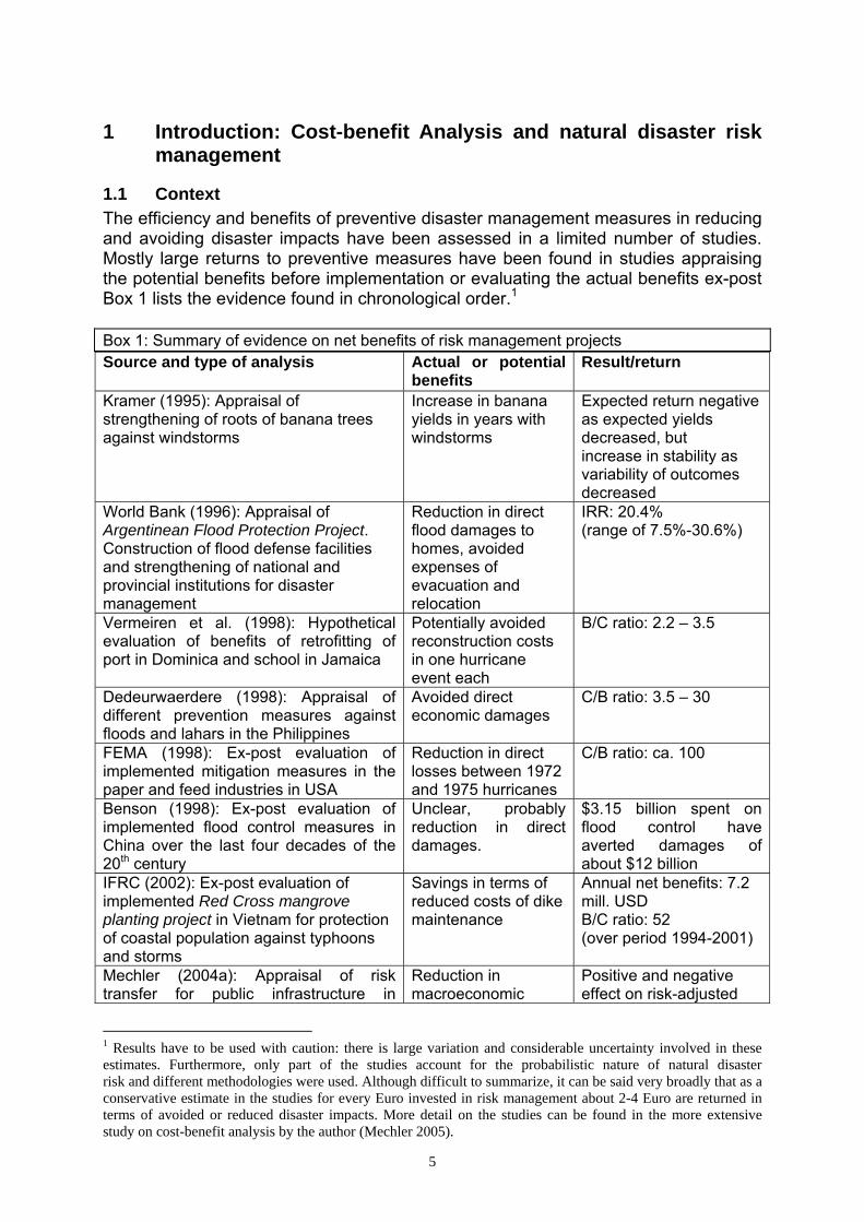
1.1 Context The efficiency and benefits of preventive disaster management measures in reducing and avoiding disaster impacts have been assessed in a limited number of studies. Mostly large returns to preventive measures have been found in studies appraising the potential benefits before implementation or evaluating the actual benefits ex-post Box 1 lists the evidence found in chronological order.1 Box 1: Summary of evidence on net benefits of risk management projects Source and type of analysis Actual or potential

benefits Result/return

Kramer (1995): Appraisal of strengthening of roots of banana trees against windstorms

Increase in banana yields in years with windstorms

Expected return negative as expected yields decreased, but increase in stability as variability of outcomes decreased

World Bank (1996): Appraisal of Argentinean Flood Protection Project. Construction of flood defense facilities and strengthening of national and provincial institutions for disaster management

Reduction in direct flood damages to homes, avoided expenses of evacuation and relocation

IRR: 20.4% (range of 7.5%-30.6%)

Vermeiren et al. (1998): Hypothetical evaluation of benefits of retrofitting of port in Dominica and school in Jamaica

Potentially avoided reconstruction costs in one hurricane event each

B/C ratio: 2.2 – 3.5

Dedeurwaerdere (1998): Appraisal of different prevention measures against floods and lahars in the Philippines

Avoided direct economic damages

C/B ratio: 3.5 – 30

FEMA (1998): Ex-post evaluation of implemented mitigation measures in the paper and feed industries in USA

Reduction in direct losses between 1972 and 1975 hurricanes

C/B ratio: ca. 100

Benson (1998): Ex-post evaluation of implemented flood control measures in China over the last four decades of the 20th century

Unclear, probably reduction in direct damages.

$3.15 billion spent on flood control have averted damages of about $12 billion

IFRC (2002): Ex-post evaluation of implemented Red Cross mangrove planting project in Vietnam for protection of coastal population against typhoons and storms

Savings in terms of reduced costs of dike maintenance

Annual net benefits: 7.2 mill. USD B/C ratio: 52 (over period 1994-2001)

Mechler (2004a): Appraisal of risk transfer for public infrastructure in

Reduction in macroeconomic

Positive and negative effect on risk-adjusted

1 Results have to be used with caution: there is large variation and considerable uncertainty involved in these estimates. Furthermore, only part of the studies account for the probabilistic nature of natural disaster risk and different methodologies were used. Although difficult to summarize, it can be said very broadly that as a conservative estimate in the studies for every Euro invested in risk management about 2-4 Euro are returned in terms of avoided or reduced disaster impacts. More detail on the studies can be found in the more extensive study on cost-benefit analysis by the author (Mechler 2005).

6

Honduras and Argentina impacts expected GDP dependent on exposure to hazards, economic context and expectation of external aid

Mechler (2004b): Prefeasibility appraisal of Polder system against flooding in Piura, Peru

Reduction in direct social and economic and indirect impacts

Best estimates: B/C ratio: 3.8 IRR: 31% NPV: 268 million Soles

Mechler (2004c): Research-oriented appraisal of integrated water management and flood protection scheme for Semarang, Indonesia

Reduction in direct and indirect economic impacts

Best estimates: B/C ratio: 2.5 IRR: 23% NPV: 414 billion Rupiah

Venton & Venton (2004) Ex-post evaluations of implemented combined disaster mitigation and preparedness program in Bihar, India and Andhra Pradesh, India

Reduction in direct social and economic, and indirect economic impacts

Bihar: B/C ratio: 3.76 (range: 3.17-4.58) NPV: 3.7 million Rupees (2.5-5.9 million Rs) Andhra Pradesh: B/C ratio: 13.38 (range: 3.70-20.05) NPV: 2.1 million Rupees (0.4-3.4 million Rs)

ProVention (2005): Ex-post evaluation of Rio Flood and Reconstruction and Prevention Project in Brazil. Construction of drainage infra-structure to break the cycle of periodic flooding

Annual benefits in terms of avoidance of residential property damages.

IRR: > 50%

Note: IRR: Internal rate of return; B/C ratio: Benefit-cost ratio; NPV: Net present value. A major decision-supporting tool commonly used for estimating the efficiency of projects is cost-benefit analysis (CBA). CBA is used to organise, appraise and present the costs and benefits, and inherent tradeoffs of projects taken by public sector authorities like local, regional and central governments and international donor institutions to increase public welfare (Kopp 1997). However, generally there is a lack of information on the costs and benefits and the profitability (net benefits) of natural disaster risk management projects:

In the absence of concrete information on net economic and social benefits and faced with limited budgetary resources, many policy makers have been reluctant to commit significant funds for risk reduction, although happy to continue pumping considerable funds into high profile, post-disaster response (Benson/Twigg 2004).

Outlining the benefits of risk management in terms of damages2 avoided and methods for including risk into project appraisal methodologies such as CBA can help changing such attitudes. There are two issues with respect to CBA in the context of efficient natural disaster risk management: 1. CBA can be used to select efficient natural disaster risk management measures in

hazard prone areas. In the context of scarce resources, CBAs are useful for selecting the most profitable projects in terms of damages avoided and rejecting those projects that are not cost-effective.

2 The terms impacts, damages, costs and losses are often used synonymously in the literature and in this report.

7

2. There is a need for incorporating disaster risk and risk management measures in project and development planning also called mainstreaming in the literature. Including disaster risk and risk management measures in appraisal methods will help rendering development more robust.

1.2 Objectives and structure This manual informs about the potential and applicability of CBA for natural disaster management in developing countries for a context with often little data and resources. The manual involved desk-based research as well as project visits to Peru and Indonesia in order to test and outline the feasibility of CBA in different contexts. Overall, the aims of this manual are: presenting methods for CBA in the context of disaster risk management in

developing countries, outlining the potential of integrating disaster risk into economic project appraisal in

order to select cost-effective projects while accounting for risk, raising awareness for the monetary dimensions of natural disaster impacts, assessing the potential and limitations for evaluating risk management projects by

means of CBA, discussing examples of benefits and costs of such projects, including net benefit

calculations. In principle, the methods discussed in this manual can be applied to the evaluation of physical risk management measures such as building a dike, as well as to “softer” ones such as implementing capacity building and people-centered early warning systems. Monetary measurement, which is at the heart of CBA, is easier for the projects with “harder” data (eg, the value of avoidance of loss of physical structures) compared to less tangible benefits such as a perceived increase in the feeling of safety due to emergency plans. This is not to say that those benefits are not of importance; to the contrary, after all the priority of disaster risk management generally is the protection of life and health. As well, methods for including non-tangible and indirect impacts exist and are discussed in the following. The manual is structured as follows: Chapter 2 discusses the basics of Cost-Benefit Analysis for natural disaster risk management such as the role of CBA in the project cycle, the steps for conducting a CBA in natural disaster risk management, important requisites, and strength and weaknesses of CBA in this context. Chapter 3 focuses in detail on the elements necessary for a CBA for natural disaster risk management. It starts with the discussion of the risk framework, describes the different kinds of impacts disasters may have and methods for measuring those, the identification of risk management projects and associated costs, and finally how to estimate their efficiency. Then Chapter 4 very concretely presents information on the necessary steps for a quantitative CBA assessment. Two quantitative frameworks are distinguished and the respective steps discussed: the risk-based forward-looking framework for quantifying risk and benefits of risk reduction, and the impacts-based, backward-looking assessment building on impacts in past disaster events. This is followed by the case studies: Chapters 5 and 6 report on the methodology used, insights gained and results of two case studies. The first study deals with the costs and benefits of flood protection schemes in Piura, Peru. The second one evaluates the case of protection

8

against tidal inundation and flooding in Semarang, Indonesia. Finally, chapter 7 concludes. Furthermore, Annex I gives an exemplary description of Terms of References for project managers for commissioning and conducting a cost benefits analysis. Annex II lists more detail on the case study in Peru.

9

2 Basics of project appraisal by Cost-Benefit Analysis for natural disaster risk management

2.1 Project cycle and project appraisal by means of Cost-Benefit Analysis When planning public investments, governments and public institutions generally are concerned with two questions: Are the net benefits due to the project positive? Does the planned project

increase public welfare, i.e. do project benefits outweigh the costs? Prioritisation: which variant of the project results in the best outcome?

CBA is the main economic project appraisal technique and commonly used by governments and public authorities for public investments. The basic idea is to render comparable all the costs and benefits of an investment accruing over time and in different sectors from the viewpoint of society. CBA has its origins in the rate-of return assessment/financial appraisal methods undertaken in business operations to assess whether investments are profitable or not. However, CBA takes a wider point of view and aims at estimating the profit for society. It is used to organise and present the costs and benefits, and inherent tradeoffs, and finally estimate the cost-efficiency of projects. The following table outlines the typical stages of a project cycle. The stages where CBA plays a role are marked in bold (table 1). Table 1: Stages of project cycle and use of CBA (in bold) 1. Programming 2. Project identification and specification 3. Appraisal: technical, environmental and economic viability 4. Financing 5. Implementation 6. Evaluation Source: Based on Benson/Twigg 2004. Projects such as investments into infrastructure or/and risk management are rooted in the context of general development programming defining guidelines, principles and priorities for development cooperation. The actual project planning starts with project identification and specification. This leads to the next, the appraisal stage where project feasibility from different perspectives is checked. Alternative versions of a project will be assessed under criteria of social, environmental and economic viability. In a fourth stage, the financing dimension of the projects will be determined which is followed by the actual implementation. Finally, projects need to be evaluated ex-post after completion in order to determine actual project benefits and whether the implemented projects did meet the expectations (Benson and Twigg 2004; Brent 1998). While CBA’s main function is to inform the appraisal stage, it is of importance for the other phases of a project cycle, specifically the project identification and specification stage (preproject appraisal stage), where it can help to preselect potential projects and reject others. Also, in the evaluation phase, CBA is regularly used for assessing if a project really has added value to society.

10

Though there are different levels of detail and complexity to CBA, the following general features and principles of CBA can be listed (box 2). Box 2: Main principles of CBA With-and without-approach: CBA compares the situation with and without the

project/investment, not the situation before and after. Focus on selection of “best-option”: CBA is used to single out the best option

rather than calculating the desirability to undertake a project per se. Societal point of view: CBA takes a social welfare approach. The benefits to

society have to outweigh the costs in order to make a project desirable. The question addressed is whether a specific project or policy adds value to all of society, not to a few individuals or business.

Clearly define boundaries of analysis: Count only losses within the geographical boundaries in the specified community/area/region/country defined at the outset. Impacts or offsets outside these geographical boundaries should not be considered.

2.2 Overview over elements of Cost-Benefit Analysis for disaster risk management

The main application of CBA in the context of disaster risk discussed here is using it for evaluating disaster risk management projects. The parts of a Cost-benefit analysis of disaster risk management are comprised of (fig. 1):

Fig. 1: Framework for estimating risk as a function of hazard and vulnerability 1. Risk analysis: risk in terms of potential impacts without risk management has to be

estimated. This entails estimating and combining hazard(s) and vulnerability. 2. Identification of risk management measures and associated costs: based on the

assessment of risk, potential risk management projects and alternatives can be identified. The costs in a CBA are the specific costs of conducting a project, which consist of investment and maintenance costs. There are the financial costs, the monetary amount that has to be spent for the project. However of more interest

11

are the so-called opportunity costs which are the benefits foregone from not being able to use these funds for other important objectives.

3. Analysis of risk reduction: next, the benefits of reducing risk are estimated. Whereas in a conventional CBA of investment projects, the benefits are the additional outcomes generated by the project compared to the situation without the project, in NDRM benefits arise due to the savings in terms of avoided direct, indirect and macroeconomic costs as well as due to the reduction in variability of project outcomes. Only those costs and benefits that can be measured likewise are included. Often, an attempt is made to monetarise those costs or benefits that are not given in such a metric, such as loss of life, environmental impacts etc. Generally, some effects and benefits will be left out of the analysis due to estimation problems.

4. Calculation of economic efficiency: Finally, economic efficiency is assessed by comparing benefits and costs. Costs and benefits arising over time need to be discounted to render current and future effects comparable. From an economic point of view, 1 $ today has more value than 1 $ in 10 years, thus future values need to be discounted by a discount rate representing the loss in value over time. Last, costs and benefits are compared under a common economic efficiency decision criterion to assess whether benefits exceed costs.

The costs and benefits of risk management projects can be illustrated as follows (fig. 2). The costs of, for example, a flood protection project are the one-time investment costs and maintenance costs that arise over the lifetime of the project. Benefits of such project arise due to the savings in terms of direct and indirect damages avoided such as avoidance of loss of life and property in the downstream area.

Fig. 2: Costs and benefits of a risk management project

12

In the context of disaster risk, benefits are probabilistic and arise only in case of events occurring, in this illustration for example with a 15% probability. This is to say, that in 85% of the cases where there are (fortunately) no disasters, no benefits due to risk management arise. Thus the viability of such a project is tied very closely to the occurrence probability of disasters. For disasters happening relatively rarely (eg. earthquakes) it may be more difficult to secure investment funds than for more frequent events such as flooding. Furthermore, the problem of proper maintenance of installed infrastructure, a general problem with public investment projects, is an additional issue if there is little awareness that a severe disaster is a real possibility. Requisites for CBA in NDRM Before engaging in and deciding upon a CBA assessment, it is necessary to clarify the objective, information needs and data situation among the different potential stakeholders such as representatives from local, regional and national planning agencies, disaster risk manager, officials concerned with public investments decisions and development cooperation staff. The specific information preferences will differ between cases involving a development bank or a municipality, between small-scale and large scale investments, planning physical infrastructure or capacity building measures, and between mainstreaming risk in CBA vs. CBA for disaster risk management. At this stage, it is paramount to find consensus among the interested and involved parties on the scope and breadth of the CBA to be undertaken. The type of envisaged product is closely linked to its potential users. CBA can be done for informational purposes, as a pre-project appraisal, as a full-blown project appraisal or as an ex-post evaluation. Purposes, resource and time commitments and expertise required differ for these products and are listed in table 2. Table 2: Characteristics of using CBAs for different purposes Product Purpose Resource

commitmentTime

commitment Expertise required

Informational study

Provide a broad overview over costs and benefits

+ Person- weeks Disaster risk management

Preproject appraisal

Singling out most effective measures for matters of more detailed evaluation in project appraisal

++ Person-months Disaster risk management,

economics

Project appraisal Detailed evaluation of accepting, modifying or rejecting project

+++ Person-months up to person-

year

Disaster risk management,

economics

Evaluation (ex-post)

Evaluation of project after completion

++ Person-months Disaster risk management,

economics

13

2.3 Strengths and limitations of Cost-Benefit Analysis There are several limitations to CBA. One is the difficulty of accounting for non-market values. Although methods exist, this involves making difficult ethical decisions, particularly regarding the value of human life. Another issue is the lack of accounting for the distribution of benefits and costs in CBA. The general principle underlying CBA is the Kaldor-Hicks-Criterion which holds that those benefiting from a specific project should potentially be able to compensate those that are disadvantaged by it (Dasgupta/Pearce 1978). Whether compensation is done in practice, however, is often not of importance. Another issue is the question of discounting benefits and costs. Applying high discount rates expresses a strong preference for the present while potentially shifting large burdens to future generations. Natural disaster risk poses additional challenges for including disaster risk into economic appraisals. Disasters are low probability, high consequence events. Their occurrence needs

to be captured by stochastic methods. This involves a solid risk assessment as the basis for assessment of benefits. This may involve considerable efforts and costs depending on the depth of the analysis to be conducted.

Planning horizons in administration are usually short, often one year whereas, as disasters are rare events, mitigation, preparedness and risk financing measures need to be planned over a longer time frame in order to accurately reflect potential benefits.

When keeping these limitations and challenges in mind, CBA is a useful tool which has its main strength that it is an explicit and rigorous accounting framework for systematic cost-efficiency decision-making. It provides a common yardstick against which the desirability of projects can be compared. It is a fact that economic efficiency is important to many decision-makers. For example, in the USA CBA considerations have "at times dominated the policy debate on natural hazards" (Burby 1991). However, CBA and economic efficiency considerations should not be the sole criterion for evaluating policies, but rather be part of a larger decision-making framework also respecting social, environmental, cultural and other considerations.

14

3 Elements for conducting a Cost-Benefit Analysis in natural disaster risk management

After having discussed the main characteristics of CBA, this chapter will lay out the basic elements of a CBA in the context of disaster risk.

3.1 Approach for estimating risk and benefits due to risk reduction Risk is commonly defined as the probability of potential impacts affecting people, assets or the environment. Natural disasters may cause a variety of effects which are usually classified into social, economic, and environmental impacts as well as according to whether they are triggered directly by the event or occur over time as indirect or macroeconomic effects (fig. 3).

Fig. 3: Natural disaster risk and categories of potential disaster impacts The standard approach for estimating natural disaster risk and potential impacts is to understand natural disaster risk as a function of hazard and vulnerability.3 Hazard analysis involves determining the type of hazards affecting a certain area with specific intensity and recurrency. In order to assess vulnerability, the relevant elements (population, assets) exposed to hazard(s) in a given area need to be identified. Furthermore, the susceptibility to damage (in the following called fragility) of those elements associated with a certain hazard intensity and recurrency needs to be assessed. Resilience decreases vulnerability and is denoted as the ability to return to pre-disaster conditions; appropriate organisational structures, know-how of prevention, mitigation ands response have a decisive influence on resilience. Combining hazard and vulnerability, results in risk and potential effects to be expected. Risk management projects aim at reducing these effects. Benefits of risk management are the reduction in risk estimated by comparing the situation with and without risk management.

3.2 Hazard Natural disaster events are commonly defined according to the underlying hazard triggering the events. There are sudden-onset events such as extreme geotectonic events: earthquakes, volcanic eruptions, landslides and slow mass movements; and extreme weather events such as tropical cyclones, floods and winterstorms. Slow-

3 More and detailed information can be found in the Risk analysis guidelines published by the GTZ (GTZ 2004).

15

onset natural disasters are either of a periodically recurrent or permanent nature such as droughts. Most disaster events are to a substantial degree caused or aggravated by human intervention (GTZ 2001). Examples are floods, landslides and forest fires. Slow-onset events are usually more significantly impacted by human behavioural patterns and there is some time for warning in advance. E.g. famines caused by droughts are an example as they are often largely a consequence of distribution bottlenecks and mismanagement in the affected regions. For these reasons famines are often treated in a different fashion than other natural disasters, and disaster management options vary from those for sudden-onset events (Sen 1999).

3.3 Vulnerability Different definitions exist for vulnerability. Vulnerability4 is a multidimensional concept encompassing a large number of factors that can be grouped into physical, economical, social and environmental factors as outlined in the chart of the GTZ Risk analysis guidelines (fig 4). The following factors affecting and comprising vulnerability can be listed: • Physical: related to the susceptibility to damage of engineering structures such as

houses, dams or roads. Also factors such as population growth may be subsumed under this category.

• Social: defined by the ability to cope with impacts on the individual level as well as referring to the existence and robustness of institutions to deal with and respond to natural disaster.

Fig. 4: Classification of vulnerability factors Source: Kohler et al. 2004. Economic: refers to the economic or financial capacity to finance losses and

return to a previously planned activity path. This may relate to private individuals as well as companies and the asset base and arrangements, or to governments that often bear a large share of a country’s risk and losses.

4 also called susceptibility or simply vulnerability in the literature.

16

Environmental: a function of factors such as land and water use, biodiversity and stability of ecosystems.

In order to operationalise and estimate vulnerability, it can be defined more narrowly as a function of: Exposure of elements such as people, assets and the environment exposed to a

hazard. Fragility: the degree of damage of elements due to the intensity of hazards.

Furthermore resilience, the ability to “bounce “back to pre-disaster conditions, is an important element of vulnerability. In contrast to exposure and fragility that focus more on the immediate impacts of disasters, resilience has a longer time frame and relates more to the secondary impacts of disasters. Furthermore, as it is harder to capture elements of resilience (such as availability of organisations and know-how to prevent and deal with disasters in quantitative terms), in this quantitatively oriented assessment it is treated with implicitly. For example the size and duration of indirect impacts strongly depends on resilience.

3.4 Overview over risk and potential impacts Combining hazard and vulnerability leads to risk and the potential impacts due to natural disasters triggered by a specific event. Risk is commonly defined as the probability of a certain event and associated impacts occurring. Potentially, there are a large number of impacts, in actual practice however, only a limited amount of those can and is usually assessed. Table 3 presents the main indicators for which usually at least some data can be found. Table 3: Summary of quantifiable disaster impacts equaling benefits in case of risk reduction

Direct Indirect Direct IndirectSocial

Number of casualties Increase of diseasesHouseholds Number of injured Stress symptoms

Number affectedEconomicPrivate sector

Households Housing damaged or destroyed

Loss of wages, reduced purchasing

powerIncrease in poverty

Public sectorEducation

HealthWater and sewage

ElectricityTransport

Emergency spendingEconomic Sectors

AgricultureIndustry

CommerceServices

Environmental Loss of natural habitats Effects on biodiversityTotal

Loss of infrastructure

services

Assets destroyed or damaged:

buildings, roads, machinery, etc.

Assets destroyed or damaged: buildings,

machinery, crops etc.

Losses due to reduced production

Monetary Non-monetary

The list of indicators is structured around the 3 broad categories social, economic and environmental, whether the effects are direct or indirect and whether they are originally indicated in monetary or non-monetary terms (table 4).

17

Table 4: Categories and characteristics of disaster impacts Categories of impacts Characteristics Direct Due to direct contact with disaster, immediate effect Indirect Occur as a result of the direct impacts, medium-long term

effect Monetary Impacts that have a market value and will be measured in

monetary terms Non-monetary Non-market impacts, such as health impacts The possibilities for monetarising non-monetary data will be discussed further below. For the purpose of this assessment referring on the project level, the macroeconomic damages are not assessed. In any way, they should not be added to direct and indirect effects as they reflect those and represent another way of looking at these effects. Social consequences may affect individuals or have a bearing on the societal level. Most relevant direct effects are the loss of life, people injured and affected, Loss of important memorabilia, Damage to cultural and heritage sites (in addition to the monetary loss).

Main indirect social effects are Increase of diseases (such as Cholera and Malaria), Increase in stress symptoms or increased incidence of depression, Disruption in school attendance, Disruptions to the social fabric,

Disruption of living environments Loss of social contacts and relationships.

Economic impacts are usually grouped into three categories: direct, indirect, and macroeconomic (also called secondary) effects (ECLAC 2003). These effects fall into stock and flow effects: direct economic damages are mostly the immediate damages or destruction to assets or “stocks,” due to the event per se. A smaller portion of these losses results from the loss of already produced goods. These damages can result from the disaster itself, or from consequential physical events, such as fires caused in the aftermath of an earthquake by collapsed power lines. Effects can be divided up into those to the private, public and economic sectors: In the private sector, the loss of and damage to houses and apartments and building contents (for example, furniture, computers) is an effect. In the public sector education facilities such as schools, health facilities (hospitals) and so-called lifeline infrastructure such as transport (roads, bridges) and irrigation, drinking water and sewage installations as well as electricity. In the economic sectors, there are furthermore damages to buildings, but most important is the loss of machinery and other productive capital. Another category of direct damages are the extra outlays of the public sector for matters of emergency spending in order to help the population during and immediately after a disaster event. The direct stock damages have indirect impacts on the “flow” of goods and services: Indirect economic losses occur as a consequence of physical destruction affecting households and firms. Most important indirect economic impacts comprise Diminished production/service due to interruption of economic activity,

18

Increased prices due to interruption of economic activity leading to reduction of household income,

Increased costs as a consequence of destroyed roads, eg. due to detours for distributing goods or going to work,

Loss or reduction of wages due to business interruption. Indirect effects represent how disasters affect the regular way of living and undertaking business. For example, in northern Peru a bridge, which had collapsed during a severe flooding event due to El Niño, was incompletely rebuilt as a pedestrian bridge. Goods now have to be brought to the bridge, carried over and put into another truck or car. Directly driving from one side of the valley to the other takes 2 hours compared to the ca. 10 minutes it took before the event. This seriously hampers the economic development of this area. For local farmers and households, this means increased efforts to sell their production or higher prices when purchasing goods. Furthermore, there are additional bottleneck effects, as the road leading over the bridge is an important thoroughfare between the second most important harbour in Peru and oil refineries to the north. Another example for indirect effects are the consequences of inundation in Indonesia caused by ground subsidence and strong rainfalls during the rainy season. Among others this seriously disrupts traffic, as trains and other means of transportation have to be rerouted. Assessing the macroeconomic impacts involves taking a different perspective and estimating the aggregate impacts on economic variables like gross domestic product (GDP), consumption and inflation due to the effects of disasters, as well as due to the reallocation of government resources to relief and reconstruction efforts. As the macroeconomic effects reflect indirect effects as well as the relief and restoration effort, these effects cannot simply be added to the direct and indirect effects without causing duplication, as they are partially accounted for by those already (ECLAC 2003).5 It should be kept in mind that the social and environmental consequences also have economic repercussions. The reverse is also true since loss of business and livelihoods can affect human health and well-being. Environmental impacts generally fall into two categories: impacts on the environment as a provider of assets that can be made use of (use values): eg. water for consumption or irrigation purposes, soil for agricultural production. These impacts are or should be taken care of in the valuation of economic impacts. The second category relates to the environment as creating non-use or amenity values. Effects on biodiversity and natural habitats fall into this category where there is not a direct, measurable benefit, but ethical or other reasons exist for protecting these assets and services.

5 There is some discussion in the literature concerning potential double-counting involved in adding direct and indirect impacts; this is due to the relation between direct impacts on stocks (quantity at a single point in time) and indirect effects on flows (services/cash flows due to using the stocks over time) (see e.g. Rose 2004; van der Veen 2004). However, this argument assumes that all direct and indirect impacts can be assessed and the cost concept used for valuing stock losses is that of the book value (purchase value less depreciation), which are not realistic assumptions for disaster impact assessment (see 3.10). In applied impact assessments and CBAs deriving order of magnitude estimates and often using reconstruction values generally direct and indirect impacts are added up (see ECLAC 2003).

19

Natural disasters often also may have positive effects such as an increase of pasture area for raising livestock, increased water availability or replenishment of aquifers. When planning preventive measures, these benefits can often be made use of and thus do not need to be subtracted. Furthermore, for example in the indirect effects on economic sectors such as agriculture (increase in livestock numbers), or in the construction sector (reconstruction boom post-event) these positive effects appear already. For this reason, and as the adverse impacts of disasters generally by far overshadow the positive effects, the positive effects are not listed separately in the following. Empirical evidence on relevance of impacts Studies on empirical evidence of disaster impacts have focussed mostly on the economic impacts and the social health effects. The general picture is that direct economic impacts are found to be increasing all over the globe mainly due to increases in welfare, strong population growth, and increasing vulnerability in many regions, whereas the losses of life remain large, but show a slightly decreasing tendency. Generally, large indirect effects are found. E.g. business interruption losses from the Northridge earthquake amounted to 6.5 billion US$ and from the Kobe earthquake to an enormous sum of 100 billion US$ (CACND 1999). The impacts of a major earthquake in 1987 in Ecuador followed by mudflows and floods on facilities of the oil-exporting industry caused direct damages (due to the costs for reconstruction of the pipelines and pumping stations as well as due to the losses of oil spilled) of ca. 120 million USD, while indirect losses amounted to ca. 165 million USD. Indirect losses comprised additional costs of investing in an alternative pipeline, greater transportation and shipping costs, cost of replacement oil export losses and lost profits (ECLAC 2004). Evidence suggests that the proportion of indirect impacts to direct impacts increases with the magnitude of the event. However, no simple relationship between direct and indirect effects has been determined so far and indirect effects are considered to be influenced by the following factors (CACND 1999): stage of development of sectors and economy, insurance penetration, financial resources available by private sector and for government assistance, specific market situation.

Studies on the economic impacts of disasters in developed countries generally do not find and discuss aggregate, macroeconomic impacts; in developing countries a series of studies focusing on developing countries find significant short- to medium-term macroeconomic effects and consider natural disasters a barrier for longer-term development (see eg. ECLAC 2003; Otero and Marti 1995).

3.5 Accounting for risk and uncertainty At this point a distinction should be made between risk and determinacy, and risk and uncertainty. In case of normal river runoffs, some small scale, gradual sedimentation may always occur. There is thus a deterministic cause-effect relationship between those two variables. The annual probability would thus be 100% equaling the certain event. In

20

case of large scale rainfalls due to El Niño (with a probability of ca. 15%, or 1-in-7 year event), excessive rainfalls will cause increased water runoffs (deterministic relationship) causing again large scale sedimentation (deterministic). As the triggering El Niño event is probabilistic, the whole chain of effects becomes probabilistic as well; these potential effects thus pose a risk. The important implication of this is that the benefits due to efforts taken to reduce the small scale sedimentation occurring annually also have probability 100% or are certain, whereas in case of the El Niño efforts for reducing large scale sedimentation will reap benefits only in case of an event, thus only on average in 15% of the years. Furthermore, if the probability of such events can be determined, one talks of risk (“measured uncertainty”); if probabilities cannot be attached to such events, this is the case of uncertainty. Disasters are infrequent events that normally cannot be forecasted, but assessed in terms of probability of occurrence. A standard statistical concept for the probabilistic representation of natural disasters is the loss-frequency function, which indicates the probability of an event not exceeding (exceedance probability) a certain level of damages. The inverse of the exceedance probability is the recurrency period, ie. an event with a recurrency of 100 years on average will occur only every 100 years. It has to be kept in mind, that this is a standard statistical concept allowing to calculate events and its consequences in a probabilistic manner. A 100 year event could also occur twice or three times in a century, the probability of such occurrences however being low. In order to avoid misinterpretation, the exceedance probability is often a better concept than the recurrency period. As an example, table 5 and figure 6 list values calculated for the case of flood risk in Piura, Peru. Table 5: Risk as represented by the loss-frequency function

Recurrency (years) Annual probability

Damages (million 2005 Peruvian Soles)

Risk: Probability*Damages

(million 2005 Peruvian soles)10 10.0% 0 0.0 50 2.0% 675 13.5 100 1.0% 1,672 16.7 200 0.5% 3,344 16.7 Annual expected damages 46.95 In this case, damages due to 10, 50, 100 and 200 year events were estimated. For example, the 100 year event, an event with an annual probability of 1%, was estimated to lead damages of ca. 1.7 billion Peruvian Soles. The last column shows the product of probability times the damages; the sum of all these products is the expected annual loss.

21

-

500

1,000

1,500

2,000

2,500

3,000

3,500

4,000

4,500

5,000

0% 1% 2% 3% 4% 5% 6% 7% 8% 9% 10% 11%

Milli

on 2

005

Sol

es

Exceedance Probability

50 year event

100 year event

200 year event

10 year eventExpected loss

Fig. 5: Example of loss-frequency distribution Another important property of loss-frequency curves is the area under the curve. This area (the sum of all damages weighted by its probabilities) represents the expected annual value of damages, i.e. the annual amount of damages that can expected to occur over a longer time horizon. This concept helps translating infrequent events and damage values into an annual number that can be used for planning purposes. Theoretically, values for a substantial number of points on the curve would be needed for matters of accuracy, generally, only a number of values will be available as in this example. Generally, disaster risk management assesses events up to 200, sometimes 500 year events. Thus, potential disaster impacts have to be understood as an approximation and uncertainty of these calculations has to be acknowledged.

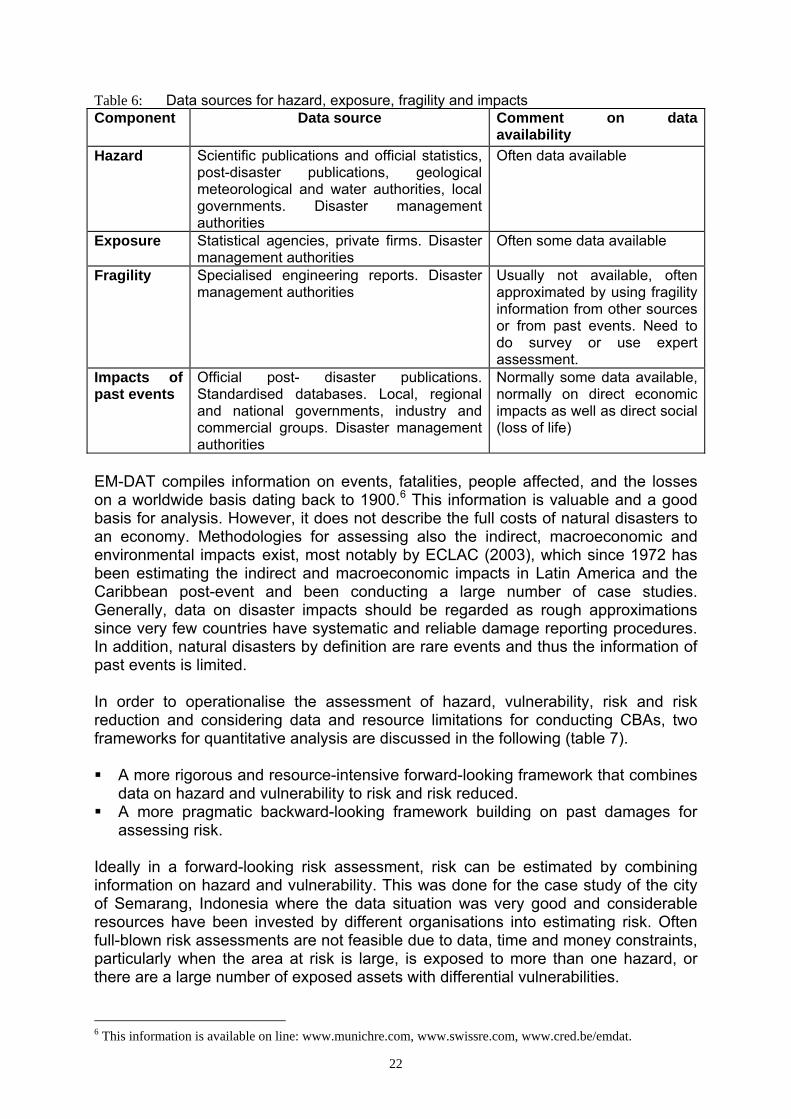
3.6 Types of assessments, requirements and data sources The type of assessment to be conducted depends upon the objectives of the respective CBA as well as the data sources at hand on hazard, vulnerability as consisting of exposure and fragility, and finally impacts. Commonly finding data on the elements of risk can be time-intensive and difficult. Particularly information on the degree of damage due to a certain hazard (fragility) is usually not readily available (see table 6). As a consequence some CBA base their estimations on past impacts and sometimes try to update these to current conditions. Estimates of damages from natural disasters often focus mainly on direct damages and loss of life, also due to the fact that there are difficulties in accounting for indirect and non-monetary damages. Direct impacts are assessed and estimated post-event by local, national, or multinational institutions and insurance companies. Main standardised databases for this information exist by Swiss Re, Munich Re, the Economic Commission for Latin America and the Caribbean (ECLAC) and the EM-DAT database from the Centre for the Epidemiology of Disasters (CRED) in Brussels. The latter is the only one that routinely also accounts for health effects, such as lives lost and people affected. Swiss Re and Munich Re annually publish data on the worldwide direct economic and insured losses.

22

Table 6: Data sources for hazard, exposure, fragility and impacts Component Data source Comment on data

availability Hazard Scientific publications and official statistics,

post-disaster publications, geological meteorological and water authorities, local governments. Disaster management authorities

Often data available

Exposure Statistical agencies, private firms. Disaster management authorities

Often some data available

Fragility Specialised engineering reports. Disaster management authorities

Usually not available, often approximated by using fragility information from other sources or from past events. Need to do survey or use expert assessment.

Impacts of past events

Official post- disaster publications. Standardised databases. Local, regional and national governments, industry and commercial groups. Disaster management authorities

Normally some data available, normally on direct economic impacts as well as direct social (loss of life)

EM-DAT compiles information on events, fatalities, people affected, and the losses on a worldwide basis dating back to 1900.6 This information is valuable and a good basis for analysis. However, it does not describe the full costs of natural disasters to an economy. Methodologies for assessing also the indirect, macroeconomic and environmental impacts exist, most notably by ECLAC (2003), which since 1972 has been estimating the indirect and macroeconomic impacts in Latin America and the Caribbean post-event and been conducting a large number of case studies. Generally, data on disaster impacts should be regarded as rough approximations since very few countries have systematic and reliable damage reporting procedures. In addition, natural disasters by definition are rare events and thus the information of past events is limited. In order to operationalise the assessment of hazard, vulnerability, risk and risk reduction and considering data and resource limitations for conducting CBAs, two frameworks for quantitative analysis are discussed in the following (table 7). A more rigorous and resource-intensive forward-looking framework that combines

data on hazard and vulnerability to risk and risk reduced. A more pragmatic backward-looking framework building on past damages for

assessing risk. Ideally in a forward-looking risk assessment, risk can be estimated by combining information on hazard and vulnerability. This was done for the case study of the city of Semarang, Indonesia where the data situation was very good and considerable resources have been invested by different organisations into estimating risk. Often full-blown risk assessments are not feasible due to data, time and money constraints, particularly when the area at risk is large, is exposed to more than one hazard, or there are a large number of exposed assets with differential vulnerabilities. 6 This information is available on line: www.munichre.com, www.swissre.com, www.cred.be/emdat.

23

Table 7: Types of assessments in context of CBA under risk and related case studies Type of assessment

Methodology Data requirements

Costs and applicability

Forward-looking assessment - risk-based Case study Semarang

Estimate hazard, vulnerability, then combine to risk

Locale and asset-specific data on hazards and vulnerability. Minimum of three data points

More accurate, but time and data-intensive (up to several person years). More applicable for small scale risk management measures, eg. retrofitting a school/building against seismic shocks Input to: Full project appraisal

Backward-looking assessment - impact-based Case study Piura

Use past damages as manifestations of past risk, then update to current risk

Data on past events, information on changes in hazard and vulnerability. Minimum of three data points (past disaster events)

Leads to rougher estimates, but more realistic and typical for developing country context. More applicable for large scale risk management measures like flood protection for river basin with various and different exposed elements. Need experience with damages in the past. Time effort: in range of several person-months. Input to: Pre-project appraisal, overview assessment

Consequently, past damages are often used as the basis for coming to an understanding of current vulnerability, hazard and potential damages. In such cases, in a backward-looking assessment past damages builds the basis to come to a rougher understanding of risk and potential damages. Such an assessment was conducted for the other case study on CBA and flood protection in the Rio Piura river basin in Peru.

3.7 Methods for assessing impacts In order to assess damages in monetary terms along the lines of the second, backward-looking approach based on reported impacts of past disasters as described above, relevant indicators of impacts need to be identified. 3.7.1 Estimating direct economic effects Generally, the prime source for past-disaster impacts are loss-assessments conducted by local, regional and national governments, industry and commercial groups and disaster management authorities. Another source of information are standardised databases on disaster losses. Mostly these sources will cover the direct economic impacts and the immediate social health consequences (in non-monetary terms). In the following, a number of important impact methods for deriving indirect economic effects as well as some techniques for deriving monetary values for social and environmental impacts are discussed. 3.7.2 Methods for deriving indirect economic effects Conventionally, the indirect effects should be assessed during a 5 year time period after an event, whereby the major ones occur during the first two years. In theory, these effects should be counted “throughout the period required to achieve the partial or total recovery of the affected production capacity” (ECLAC 2003). As a general characteristic, indirect effects tend to be prevail longer in developing countries than in more developed ones. These indirect effects can be estimated after an event by

24

Conducting surveys post event: bottom-up, Examining statistical information on the performance of affected sectors after the

event in top-down manner, Deriving simple relationships.

These different approaches are discussed in the following. Method 1: Estimating past indirect economic effects through a survey (bottom-up approach) Indirect effects can be measured by a survey post-event. This involves addressing those people and businesses that were mainly affected, collecting their responses and summarising the results. As the assessment focuses on the individual impacts on the ground, this is a so-called bottom-up assessment. A number of effects may be crucial, the selection of the relevant ones depends on the specific impacts of a disaster and the selection remains at the discretion of those that conduct such a survey. For example, indirect effects in terms of traffic interruption due to destroyed roads or damaged bridges may comprise the following (ECLAC 2004): - costs of operating additional trains in the emergency period and of post-emergency train service - The increased operating costs for vehicles making a detour, - Profits forgone due to cancelled long-distance trips, - Greater operating costs for local traffic, - Loss of profits due to local trips cancelled, - Greater operating costs due to damage to the surface of alternative roads, - Longer journey times for people who changed from buses to trains, - Reduced operating costs for buses due to transfers to trains during the emergency, and - Reduced operating costs for buses due to transfers to trains in the post-emergency stage - Change in volume of traffic: reduction of traffic due to increased costs. Method 2: Estimating indirect effects from past statistical information (top-down approach) In contrast to the bottom-up approach, a top-down assessment starts from a more aggregate level analysing data of official statistics. An important issue is that this method for estimating indirect economic effects entails comparing the economic situation with a disaster to the situation without it (see eg. ECLAC 2003). As the situation that would have materialized absent a disaster is unknown, there is the necessity to derive a fictitious estimate of what would have happened if a disaster had not occurred. Basically the following steps need to be taken: Assessment of pre-disaster situation in order to determine average growth in pre-

disaster context, Conduct forecast based on average growth for a hypothetical post-disaster

situation without disaster, Assess actual post-disaster situation, Compare hypothetical and actual post-disaster situation and baseline leading to

indirect effects. For example, assume a disaster hit a certain region in 1995 destroying crops and seedlings. Agricultural production in this sector will fall behind planned production

25

without a disaster. In this case, the indirect effects would be the output reduction for as long as the effects last (fig. 6).

indirect losses

Agricultural sector in region X

507090

110130150170

1990

1991

1992

1993

1994

1995

1996

1997

1998

1999

2000

Con

stan

t LC

Uwithout disasterwith disaster

Fig. 6: Assessing indirect losses in theory by top-down method The indirect loss is the difference between the hypothetical case without a disaster (value added keeps growing with same pre-disaster rate) and the actual performance. In practice, the estimation is more difficult. Main issues are the isolation of disasters effects from other influences as well as the question of duration of effects. Eg. looking at the agriculture, livestock and forestry sector in Piura, we can clearly discern the effects of the El Niño 1982/83 and 1997/98. However, the question is what to count as an indirect effect. • In 1983 agricultural output decreased strongly after it had been stagnant before; in 1984 and onwards it increased again. An issue is whether this was due to the El Niño? • In 1998 it again decreased after there had been an upward trend in value added, and in 1999-2001 output stagnated; an issue is whether the stagnation was caused by El Niño?

Agriculture, livestock and forestry

-200400600800

1,0001,2001,4001,6001,800

1970

1971

1972

1973

1974

1975

1976

1977

1978

1979

1980

1981

1982

1983

1984

1985

1986

1987

1988

1989

1990

1991

1992

1993

1994

1995

1996

1997

1998

1999

2000

2001

Mill

ion

New

Sol

es 2

004

FEN 97/98

FEN 82/83

Fig. 7: Assessing indirect losses in practice: development of agricultural value added in Department of Piura 1970-2001 In such cases, a conservative approach is required considering only those effects that can be attributed with relative certainty to the extreme event. Here one would only use the shortfalls in agricultural output in 1983 compared to 82 and 1998 to 1997 to be on a relatively safe side. This outlines some of the problems with estimating indirect effects after an event and demonstrates that it is often difficult to isolate the impacts due to disasters from other influences. Thus, such estimates (as all damage estimates!) have to be used with some amount of caution.

26

Method 3: Estimating indirect effects due to business interruption Parker et al. 1987 offers a simple formula for assessing the indirect loss (L) due to business interruption as the product of a company’s/sector’s typical daily gross profit (GM) times the days (D) that production has been interrupted:

L=GM*D where L: indirect loss, GM: daily gross profit, D: days interrupted. However, information on gross profit margin as well as days of production interruption is necessary. What concerns time of production interruption there is a wide variation reported in the literature. Parker et al. report (for a developed country context) that whereas clean-up after a disaster will take a maximum of two weeks, machinery replacement may take from one day to one year and stock replacement from a few hours up to six months. 3.7.3 Monetarising non-monetary impacts

3.7.3.1 Methods for valuation of non-monetary effects If goods and services are not traded in the market, there will generally be no monetary value for it. Most social and environmental impacts such as the loss of human lives, injuries and psychological post-disaster trauma, environmental impacts such as loss of arable land, forests and habitats due to disasters fall into this category and for these nor reconstruction or repair costs do exist. For these impacts, values need to established for later usage in a CBA. Generally the procedure to be followed is two-fold

1. First, estimation of physical value: number of incidences, eg. how many affected people etc.

2. Attaching a monetary value to the physical value. There is a large literature on the monetarisation of non-market impacts, particularly driven by the application of CBA in the field of environmental economics. Methods can be broken down into indirect and direct methods (figure 8).

27

Fig. 8: Methods for monetarising benefits Source: Own illustration after Endres/Staiger 1995; Hanley/Spash 1993. Direct preference assessment is done by means of contingent valuation where orally or in written form subjects are surveyed and their preferences determined (e.g. willingness to accept a change in the environment, willingness to pay for avoiding premature death). One important application is the valuation of life (Value of a Statistical Life (VSL)) that is based on assessing the willingness to pay for avoiding premature death. A major problem is the resulting differential in values between developed and less-developed countries as the willingness to pay is proportional to income. The indirect method estimates the value attached to risk reduction based on actual market behaviour, eg. the medical costs for treating a disease or the income lost due to disease or death. Relevant methods are the analysis of substitution relationships (measuring extra efforts undertaken to mitigate adverse impacts, such as installing soundproof windows for reducing noise levels), the travel cost method (the travel cost incurred to make use of environmental amenities such as lakes and natural parks) and hedonic pricing (eg. the change over time of property prices in reaction to change in environmental conditions).

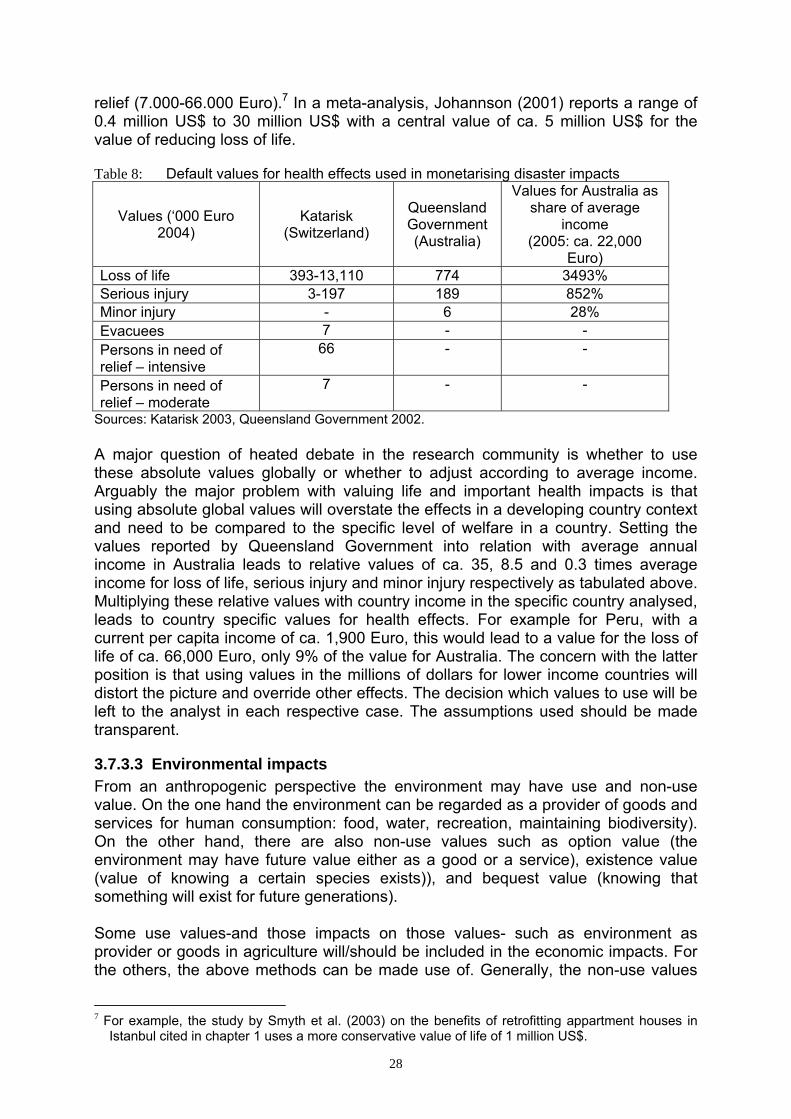
3.7.3.2 Social effects After estimating social effects in physical terms, monetary values can be attached to important impacts. As this is generally a contentious issue and not often done, only a few studies on natural disaster impacts discuss and list values for such impacts. For the more serious effects loss of life, serious and minor injury, Queensland Government (2002) lists values of 774.000, 189.000 and 16.000 Euro, which are broadly in line with values of other studies. The Swiss study Katarisk reports a large range for loss of life (393.000-13.100.000 Euro) and serious injury (3.000-197.000 Euro) as well as values for cost of evacuation (7.000 Euro) and persons in need or

28

relief (7.000-66.000 Euro).7 In a meta-analysis, Johannson (2001) reports a range of 0.4 million US$ to 30 million US$ with a central value of ca. 5 million US$ for the value of reducing loss of life. Table 8: Default values for health effects used in monetarising disaster impacts

Values (‘000 Euro 2004)

Katarisk (Switzerland)

Queensland Government (Australia)

Values for Australia as share of average

income (2005: ca. 22,000

Euro) Loss of life 393-13,110 774 3493% Serious injury 3-197 189 852% Minor injury - 6 28% Evacuees 7 - - Persons in need of relief – intensive

66 - -

Persons in need of relief – moderate

7 - -

Sources: Katarisk 2003, Queensland Government 2002. A major question of heated debate in the research community is whether to use these absolute values globally or whether to adjust according to average income. Arguably the major problem with valuing life and important health impacts is that using absolute global values will overstate the effects in a developing country context and need to be compared to the specific level of welfare in a country. Setting the values reported by Queensland Government into relation with average annual income in Australia leads to relative values of ca. 35, 8.5 and 0.3 times average income for loss of life, serious injury and minor injury respectively as tabulated above. Multiplying these relative values with country income in the specific country analysed, leads to country specific values for health effects. For example for Peru, with a current per capita income of ca. 1,900 Euro, this would lead to a value for the loss of life of ca. 66,000 Euro, only 9% of the value for Australia. The concern with the latter position is that using values in the millions of dollars for lower income countries will distort the picture and override other effects. The decision which values to use will be left to the analyst in each respective case. The assumptions used should be made transparent.

3.7.3.3 Environmental impacts From an anthropogenic perspective the environment may have use and non-use value. On the one hand the environment can be regarded as a provider of goods and services for human consumption: food, water, recreation, maintaining biodiversity). On the other hand, there are also non-use values such as option value (the environment may have future value either as a good or a service), existence value (value of knowing a certain species exists)), and bequest value (knowing that something will exist for future generations). Some use values-and those impacts on those values- such as environment as provider or goods in agriculture will/should be included in the economic impacts. For the others, the above methods can be made use of. Generally, the non-use values

7 For example, the study by Smyth et al. (2003) on the benefits of retrofitting appartment houses in

Istanbul cited in chapter 1 uses a more conservative value of life of 1 million US$.

29

are more difficult to assess and contingent valuation methods are used here for eliciting values. Little evidence was found on employing methods for valuing disaster impacts on the environment. One example documented in Penning-Rowsell et al. uses both the Contingent Valuation and travel cost methods for deriving the benefits of recreational value of a certain area of coastline in England and the benefits of efforts for stopping coastal erosion affecting this coastline. This considerable research effort involved devising a questionnaire and asking ca. 400 groups comprising of 1500 people. A total value of 191,000 Pounds was estimated for maintaining access to the area. As a general proposition, the valuation of environmental impacts is highly case-specific, default values (such as for the health impacts) can rarely be used and there will be need to involve specialists for applying the discussed methods.

3.8 Identification of risk management measures and costs There is a wide spectrum of potential mitigation, preparedness and risk financing measures that can be taken in order to reduce or finance risk. Table 9 lists a selection of these risk management measures that reduce risk (mitigation and preparedness) or transfer and spread it to a larger basis (risk financing). Table 9: Overview over risk management measures

Risk reduction Mitigation/prevention Preparedness

Risk financing

Physical and structural mitigation works

Early warning systems, communication systems

Risk transfer (by means of (re-) insurance) for public infra-structure and private assets

Land-use planning and building codes

Contingency planning, networks for emergency response

Alternative risk transfer

Economic incentives for active risk management

Shelter facilities, evacuation plans

National and local reserve funds

Education, training and awareness

Source: Based on IDB 2000. Risk management measures mainly focus on reducing vulnerability. Although, the underlying economic and risk assessment principles to be used for a CBA are generic, different hazards and thus disasters have differential suitability for being analysed in terms of risk or uncertainty and for applying mitigation measures as shown in a table in the report by the Queensland Government (2002). There are important differences related to: Hazard characteristics: hazard warning times can be long (days for cyclones) or

zero (for earthquakes). The attributes relating to the size/extent of the hazard can vary, making it difficult to estimate likely direct losses – such as flood water depths and velocities, wind speeds, earthquake magnitude etc.

Assessing exposure and vulnerability: potential exposure of people and assets may be difficult to determine for some hazards, for example if there is no history of past events. As discussed, fragility is only rarely assessed quantitatively.

30

Probabilistic information: for some sudden-onset events like earthquakes probabilistic analyses are rather difficult to conduct (due to lack of past data etc.).

Loss assessment: as discussed loss assessments are difficult to compare, and different methods are often used.

Mitigation options: these differ between hazards. While for floods a wide array of options are available, these are more limited for severe storms and earthquakes.

The costs in a CBA are the specific costs of conducting a project. Usually there are major initial outlays for the investment effort such as building a dike, followed by Smaller maintenance expenses occurring over time, eg for maintaining a dike.

On the other hand, risk financing measures usually demand a constant annual payment, e.g. insurance premium guaranteeing financial protection in case of an event. These costs normally can be determined in a straightforward manner as market prices exist for cost items such as labour, material and other inputs. Some uncertainty in these estimates usually remains as prices for inputs and labour may be subject to fluctuations. Often, project appraisals make allowance for such possible fluctuations by varying cost estimates by a certain percentage compared to the best estimate when estimating the costs.

3.9 Estimating efficiency of NDRM The final step in a CBA is to compare costs and benefits and calculate the efficiency of the analysed options. There are two steps for doing so. First benefits arising over time need to be discounted, then project evaluation decision criteria are applied in order to calculate the efficiency. Discounting In a CBA (and economics in general), costs and benefit streams occurring in future periods need to be discounted. This entails adjusting future benefits and costs by the discount factor (1+r)t, whereby r signifies the social discount rate and t is the time index. Discounting is undertaken as people put a higher value on the present, funds invested now offer profit opportunities in the future (thus, there are so-called opportunities costs to using funds for other purposes) and there is generally uncertainty about the future. The discount rate represents the average return of a public investment into alternatives projects. Eg. a discount rate of 12% signifies that investing public funds (into water infrastructure, health, education etc.) on average would bring about a return of 12% and other projects would need to have at least an equal return in order to be considered. Often a discount rate of 12% is chosen in practical applications for the calculation of the NPV, e.g. standard used by Asian Development Bank (ADB 2001). However, sensitivity analysis should be done to assess the influence of varying this parameter for different countries with different conditions. Project evaluation decision criteria Finally, costs and benefits have to be compared under a common efficiency criterion in order to be able to derive at a decision. Basically, three decision criteria are of major importance in CBA: Net present value (NPV) Criterion: costs and benefits arising over time are

discounted and the difference taken, which is the net discounted benefit in a given

31

year. The sum of the net benefits is the NPV. A fixed discount rate is used to represent the opportunity costs of using the public funds for the given project. If the NPV is positive (benefits exceed costs), then a project is considered desirable.

The CB-Ratio Criterion is a variant of the NPV: The benefits are divided by the costs. If the ratio is larger than 1, i.e. benefits exceed costs, a project adds value to society.

Internal Rate of return (IRR) Criterion: Whereas the former two criteria use a fixed discount rate, this criterion calculates the interest rate internally which represents the return of the given project. A project is rated desirable if this IRR surpasses the average return of public capital determined beforehand (eg. 12%).

In most circumstances, the three methods are equivalent. Overall however, the NPV method is the preferred criterion (Zerbe and Dively 1994; Dasgupta and Pearce 1978; Brent 1998).

3.10 Prices and inflation adjustment There are a number of issues related to measuring effects in monetary values which should be kept in mind and understood as they may have substantial impact in values calculated. Cost concepts One issue is which cost concept to use. This relates mostly to the direct asset losses which will be needed to be replaced. In theory, damages can be assessed in purchase prices, i.e. prices to which assets/goods were purchased, current value prices (book value), i.e. purchase value less depreciation, or replacement costs.

In most cases, current value prices will be smaller than purchase prices as the depreciation in value is factored in already. It is not clear whether replacement costs will be higher than purchase prices as prices for certain assets may have decreased or increased. From a theoretical economic point of view, losses to assets should be valued in current value prices. However, with high inflation rates typical for developing countries these book values may underrepresent actual value. In such cases, replacement costs may be a good proxy. On the other hand, it may often be easier and quicker to use purchase prices (adjusted for inflation) as documentation of those will usually be available. The use of these concepts again depends on data availability and purposes of the assessment. In published reports on direct damages, often the type of cost concept used is not revealed explicitly. Adjusting for inflation When assessing past and present damages, it is important to relate measured values to a common base year. This is an important issue that is often neglected in damage assessments where current prices of the time of the disasters are used leading to a large understatement of actual impacts. Very often it is however unclear to which base year damage estimates listed in statistics refer to. Furthermore, price deflating, or indicating prices in constant terms related to a specific base year, needs to be done in order to be able to compare potential losses with the costs of preventive measures that are planned and paid for in current values. The relationship between current and constant prices and the price index is as follows.

32

Pco=Pcu/(Pi/100) where Pco: constant prices, Pcu: current prices, Pi: price index Price indexes are regularly published by national statistical institutes and international institutions such as the World Bank for households (consumer price index), different economic sectors and GDP. However, for calculating values in constant prices of the current year, the appropriate deflator will usually be missing, so one needs to make assumptions, such as inflation in the current year is equal to inflation in the past year. The following table shows how to use price indexes in order to calculate constant values. Table 10: Using deflators to adjust from current to constant prices (Peru)

Year Price index (base year 1990=100)

Change in price index =annual Inflation

Price index (base year 2005=100)

1990 100 - 4 1991 480 379.9% 19 1992 812 69.2% 33 1993 1,194 47.1% 48 1994 1,506 26.2% 61 1995 1,701 12.9% 69 1996 1,880 10.5% 76 1997 2,023 7.6% 82 1998 2,153 6.4% 87 1999 2,238 3.9% 91 2000 2,320 3.6% 94 2001 2,349 1.3% 95 2002 (assumption) 2,380 1.3% 96 2003 (assumption) 2,410 1.3% 97 2004 (assumption) 2,441 1.3% 99 2005 (assumption) 2,472 1.3% 100 Data source: World Bank 2003. Note: No data were available for the years 2002-2005, thus the assumption was taken that inflation would stay constant after 2001 at 1.3%. In the first column, a price index (in this case for GDP) with the base year 1990 (=100) is given. The price level in the years up to 2005 is thus listed in constant prices of 1990, thus the value of 2472 in the year 2005 indicates an inflationary trend from 1990 to 2005 of ca. 2,400% (fig. 9)

33

-

500

1,000

1,500

2,000

2,500

1990

1991

1992

1993

1994

1995

1996

1997

1998

1999

2000

2001

2002

2003

2004

2005

1990=100

Fig. 9: Price development in Peru since 1990 A value of 2,472 Soles in current prices of today would be equal to a value of 100 Soles in 1990. Annual inflation is the change in the price index listed in the next column. With a given price index it is easy to change the base year. For example in column 3, the base year is changed to 2005, by dividing the time series by 24.72 (2472/100, the price level in 2005 by the price level in 1990).

3.11 Distribution of impacts Whereas the project costs- if financed by a loan- are distributed relatively equitably over the population (new debt that will be paid back with taxpayers money), the distribution of benefits tends to be more complex. In the case of new project being planned, there may be different perceptions which of the risks need to be addressed and what the benefits of projects may be.

Measurement is further complicated by the fact that one needs to take into account the fact that different groups attach different values to various forms of risk. For instance, a national government may view the loss of a hospital in purely monetary terms. For a local community, the loss will be felt very differently, potentially jeopardising the lives of themselves and their loved ones with a wide range of consequences, not least for livelihood security (Benson/Twigg 2004).

It may be important to assess who is affected be it households, the public sector or the business sector. Also among those groups, it is of interest how losses are distributed, eg. whether poor farmers or households are affected the most or whether the burdens are shared relatively equally. Empirical evidence shows that there is increasing utility to benefits with decreasing income. In very broad terms, this evidence suggests that an extra Euro to someone earning 1000 Euro is worth twice as much as to someone receiving 2000 Euros a year (UK Treasury 2003). There have been efforts to use weights for project impacts according to income distribution, however information on the income group distribution of effects is often not readily available and analytical derivation has been proven to be very difficult, so the distributional side has been neglected.

34

3.12 Additional benefits of NDRM Often disaster risk management projects are not undertaken in isolation, but rather combined with other considerations bringing about improvements in conditions. For example, flood protection structures may at the same time be used to provide irrigation or drinking water and electricity. For example, in the case of the Polder in Piura, flood waters diverted into the Polder retention basin, will be used for irrigation purposes in an area that generally lacks sufficient irrigation. In Semarang, a dam is planned upstream of a major river for flood control purposes, but as well for water supply purposes (the major developmental issue) and hydroelectricity generation.

3.13 Uncertainty of estimations Estimating the benefits of risk reduction is associated with a substantial amount of uncertainty, particularly so as disasters are by definition low-frequency events and thus little data exist. Uncertainties are inherent in The recurrency of hazards: estimates are often based on a limited number of data

points only. Incomplete damage assessments: data will not be available for all relevant direct

and indirect effects, particularly so for the non-monetary effects. Double-counting: For example counting crop losses in agriculture twice as a direct

(stock) and indirect (flow) impact. Fragility: fragility curves do often not exist and standard ones have to be applied. Exposure: the dynamics of population increase and urban expansion, increase of

welfare need to be accounted for and forecast to the future. Benefits of risk management estimates: often difficult to accurately measure the

effect and benefit of risk management measures. Value of life estimates and other adverse health effects: large uncertainty about

values, as well as debate whether to use global, higher or national values that reflect differences in per capita income

Discounting: the discount rate used reduces benefits over the lifetime of a project and thus has very important impact on the result.

There are calculation issues related to the exchange rates, deflators and cost concept used.

When deriving a probability distribution by a limited number of data points losses may be overestimated or underestimated relative to the “true” loss probability relationship. Of course, in practice the “true” relationship is never known. What the chart demonstrates is that with increasing data points, the approximation to the underlying relationship is bound to get better. However, as discussed (and further elaborated in the case studies) often the number of data points that can be derived is limited due to lack of data and time and money constraints. Estimates of risk and benefits of risk reduction should be understood in terms of orders of magnitude. Sensitivity analysis should generally be conducted to study the robustness of results to changes of important assumptions or methodology. Sensitivity analysis Generally, it is difficult to assess uncertainty in quantitative terms. For this matter, a useful method is sensitivity analysis where assumptions and values are changed in

35

and ad-hoc manner. For example, in the case study on flood protection in Piura, Peru sensitivity analyses were conducted as follows: Increasing costs ad-hoc by 30%, eg. due to unforeseen price increase in labour or

material inputs. Not taking account of loss of life. Not taking account of indirect effects. Not taking account of increases in exposure.

This led to the following effects on the internal rate of return (IRR).

0%5%

10%15%20%25%30%35%

IRR

Bestestimate

Costs:+30%

Withoutloss of life

Withoutindirectimpacts

Withoutincreases

inexposure

Fig. 10: Sensitivity analysis for the case of Piura Compared to the IRR of the base case (“best estimate”), the IRRs significantly decreased for the cases with an increase in costs and the case without accounting for indirect impacts. However, for all cases, the IRRs remained above the 12% threshold.

36

4 Quantitative frameworks for estimating risk and risk reduction After the discussion on risk and potential impacts, this part will outline how to approach the estimation and monetary quantification of disaster risk for the purposes of a CBA by means of the two frameworks distinguished above: The more rigorous framework combining data on hazard and vulnerability to an

estimate of risk and risk reduced (forward-looking, risk-based approach) The more pragmatic framework relying on past damages (backward-looking,

impact-based) The appropriate approach to be used depends on the objectives of the specific CBA conducted, the data situation and available resources and expertise. In the following, these frameworks will be discussed and important indicators for measuring hazard, vulnerability and finally risk and impacts outlined. Furthermore, the scope for quantifying and monetarising those will be assessed. The steps discussed in the following refer to part 1: risk analysis and part 3: analysis of risk reduction outlined in chapter 2.

4.1 Forward-looking framework (risk-based) For measuring risk and the benefits arising due to risk reduction in a quantitative manner, there are 4 steps to be followed (fig. 11), of which the first three steps correspond to the risk analysis process with the hazard, vulnerability and risk assessments. Based on this, in a fourth step the benefits due to risk reduction can be determined. In detail, the necessary steps are:

37

Hazard intensityEg water level

Damages

Hazard intensityEg water level

Damages

Step 1: Hazard analysis

Step 2: Vulnerability analysis- exposure- fragility

Step 3: Risk analysis: Probability * Damages

Step 4: Analysis of benefits of risk reduction:

Probability * Damages reduced

Benefits of risk reduction

Original loss-frequency curve

Loss-frequency curve with risk reduction

Damages

Exceedance probability

Exceedance probability

Exceedance probability(inverse: recurrency period)

Fig. 11: Quantitative forward-looking framework for estimating disaster risk Illustration modified based on World Bank 1996. Step 1) Hazard analysis Outcome: intensity and recurrency of natural phenomenon This involves assessing the probability of certain hazard intensity at a given location. Hazard intensity can be measured eg. by water inundation levels or stream flows at a location in a river basin, seismic ground motion as measured by the Mercalli scale, or hurricane intensity. A common statistical concept for measuring the probability of hazards occurring is the recurrency period describing the average period with which an event of similar magnitude will occur again in the future. For example, chart 12 shows the probability of water depths exceeding certain levels at a location alongside the river Garang in the city of Semarang, Indonesia.

38

-

0.5

1.0

1.5

2.0

2.5

3.0

0% 2% 4% 6% 8% 10% 12% 14% 16% 18% 20%Exceedance probability

flood

dep

th (m

)

Fig. 12: Probability of flood depths in Semarang Step 2) Vulnerability analysis Outcome: degree of damage due to hazard intensity This involves estimating the exposed population and assets as well as the degree of damage and total damages to the population and those assets as a function of the hazard intensity Exposure In the exposure analysis, geographical area and elements exposed to the relevant hazard(s) need to be identified and estimated quantitatively. This involves determining • Population living in the area, • Number and value of assets, such as private houses, public buildings, factories,

small scale business, environmental land use etc. For such an analysis, often values per m2 (unit values) are used. For example, in the Semarang case a GIS-based exposure database and map was created allowing to determine the area, population and crucial assets that may be affected by the relevant hazards. Furthermore, unit values for land-use categories such as residential housing, business or commercial uses were determined and integrated in the database.

Generally, exposure analysis needs to look into the future and estimate exposure in the future. If there is a constraint on data, or the situation is relevant static (stable population, little migration), then it can be assumed that current exposure is equal to future exposure. On the other hand, if it is clear, that the exposure is highly dynamic, it should be accounted. An easy method is to calculate an annual growth rate for population and assets. Generally, some information on population growth in the past and future will be available in statistics and/or reports. For assets, this is normally more difficult. A relatively robust, simplifying assumption could is to assume that asset growth is proportional or equal to population growth.

39

Fig. 13: Example of exposure map for the case study of Semarang Fragility In a next step, fragility as the degree of damage of the exposed elements can be estimated, eg. the fragility/damage proportion of a bridge to certain flood levels or the fragility of a certain class of buildings to seismic ground motion. Typically damage costs are elicited for a certain (class of) assets as a function of hazard intensity. If possible, such assessments should be conducted locale-and asset-specific, eg. for bridges or for a type of residential building. Fragility functions may look like the following ones used in the case study on flooding in Semarang.

0%

2%

4%

6%

8%

10%

12%

14%

16%

18%

- 0.2 0.4 0.6 0.8 1.0 1.2 1.4 1.6 1.8 2.0 2.2 2.4 2.6 2.8 3.0

Residential IndustriesBusiness Indirect business lossesVegetation and farmland

Dam

age

ratio

Flood depth (m)

Fig. 14: Fragility: degree of damage as a function of hazard intensity The degree of direct and indirect damage is increasing with increasing flood depth. Often, the lack of availability of such fragility is a major constraint in risk and damage

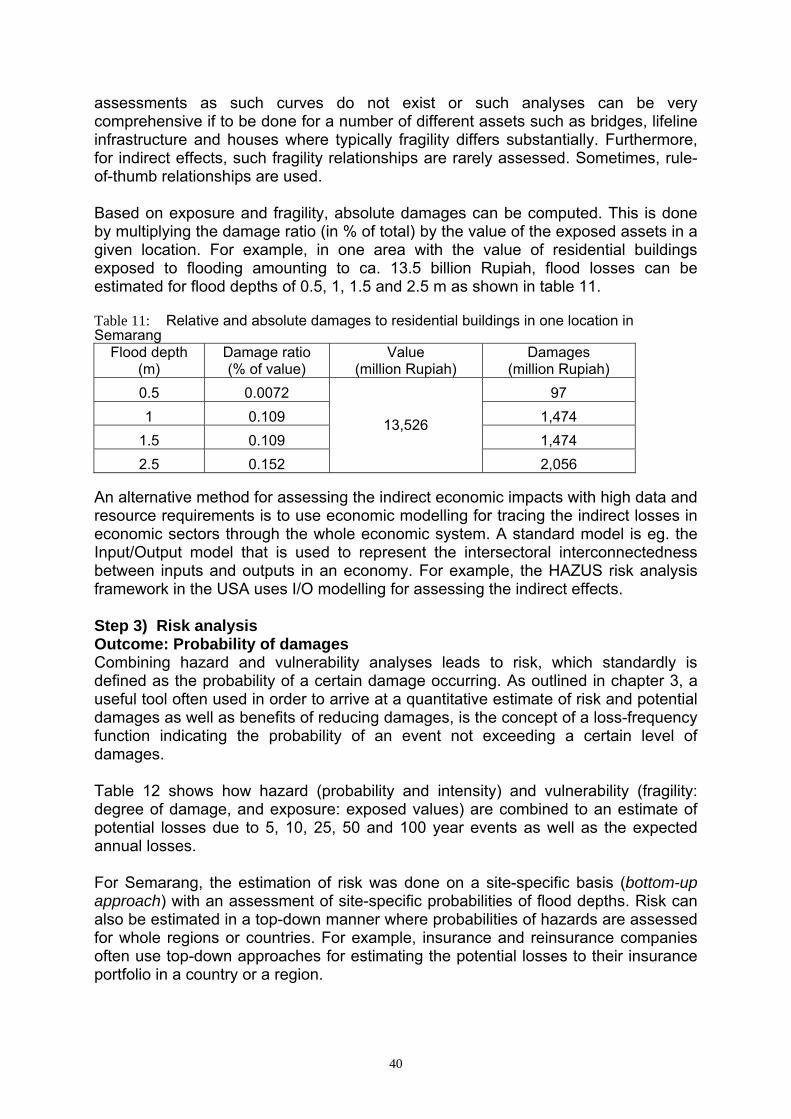
40

assessments as such curves do not exist or such analyses can be very comprehensive if to be done for a number of different assets such as bridges, lifeline infrastructure and houses where typically fragility differs substantially. Furthermore, for indirect effects, such fragility relationships are rarely assessed. Sometimes, rule-of-thumb relationships are used. Based on exposure and fragility, absolute damages can be computed. This is done by multiplying the damage ratio (in % of total) by the value of the exposed assets in a given location. For example, in one area with the value of residential buildings exposed to flooding amounting to ca. 13.5 billion Rupiah, flood losses can be estimated for flood depths of 0.5, 1, 1.5 and 2.5 m as shown in table 11. Table 11: Relative and absolute damages to residential buildings in one location in Semarang

Flood depth (m)

Damage ratio (% of value)

Value (million Rupiah)

Damages (million Rupiah)

0.5 0.0072 97 1 0.109 1,474

1.5 0.109 1,474 2.5 0.152

13,526

2,056 An alternative method for assessing the indirect economic impacts with high data and resource requirements is to use economic modelling for tracing the indirect losses in economic sectors through the whole economic system. A standard model is eg. the Input/Output model that is used to represent the intersectoral interconnectedness between inputs and outputs in an economy. For example, the HAZUS risk analysis framework in the USA uses I/O modelling for assessing the indirect effects. Step 3) Risk analysis Outcome: Probability of damages Combining hazard and vulnerability analyses leads to risk, which standardly is defined as the probability of a certain damage occurring. As outlined in chapter 3, a useful tool often used in order to arrive at a quantitative estimate of risk and potential damages as well as benefits of reducing damages, is the concept of a loss-frequency function indicating the probability of an event not exceeding a certain level of damages. Table 12 shows how hazard (probability and intensity) and vulnerability (fragility: degree of damage, and exposure: exposed values) are combined to an estimate of potential losses due to 5, 10, 25, 50 and 100 year events as well as the expected annual losses. For Semarang, the estimation of risk was done on a site-specific basis (bottom-up approach) with an assessment of site-specific probabilities of flood depths. Risk can also be estimated in a top-down manner where probabilities of hazards are assessed for whole regions or countries. For example, insurance and reinsurance companies often use top-down approaches for estimating the potential losses to their insurance portfolio in a country or a region.

41

Table 12: Calculating site-specific risk in Semarang

Recurrrency (years)

Annual probability

Intensity (flood depth in m)

Fragility: Damage ratio

Exposure: (million Rupiah)


Risk: Probability*damages (million Rupiah)

5 20% 0.3 0.0% 0.00 0.0010 10% 0.5 0.7% 97.39 9.7425 4% 1 10.9% 1,474.33 58.9750 2% 1.5 10.9% 1,474.33 29.49

100 1% 2.5 15.2% 2,055.95 20.56118.76

Annual expected losses

13,526

RiskHazard Vulnerability

Calculating site-specific risks for all relevant locations in this manner and aggregating leads to the total losses in the exposed area and it is indicated in figure 15. Step 4) Analysis of risk management project. Outcome: Net benefits due to reduction of potential damages The benefits due to risk management measures are the avoided and reduced losses; graphically, this is here represented in shifting the loss-frequency curve downwards. In the example shown in figure 15, losses up to the 100 year event would be avoided.

-

500

1,000

1,500

2,000

0% 2% 4% 6% 8% 10% 12% 14% 16% 18% 20% 22% 24%

Damages

Damages with risk management project

Billi

on R

upia

h


Benefits of risk management: risk/potential damages reduced

Fig. 15: Benefits due to reducing risk and potential damages The area between the two curves represents the expected annual damages reduced or expected annual benefits due to risk management.

4.2 Backward-looking assessment (impact-based) In a less rigorous and less data-intensive backward-looking assessment past damages build the basis for a rougher understanding of risk and potential damages. Such an assessment was conducted for the case of CBA of flood protection in Piura.

42

Damages

Benefits of risk reduction

Original loss-frequency curve

Loss-frequency curve with risk reduction

Damages



Step 1: Assessment of past damage events


Health HealthHouseholds Sense of Insecurity

EconomicPrivate sector


Eg loss of wages, reduced purchasing


Public sector and Infrastructure

EducationHealth

Water and sewageElectricityTransport


AgricultureIndustry

Commerce…

EnvironmentalLoss of natural habitats Loss of services

Reduction/loss of infrastructure services and/or increased cost


roads, machinery, etc.

Assets destroyed or damaged: buildings, machinery, crops etc.

Indicated in monetary terms Indicated in non-monetary terms

Profit losses due to reduced production

Recorded Impacts in past events

Step 2: Accounting for possible changes in exposure and vulnerability

Probability of occurrenceor recurrency period

Original curve

Downward shift due to flood protection

Increase in damages due to increased exposure


Health HealthHouseholds Sense of Insecurity

EconomicPrivate sector


Eg loss of wages, reduced purchasing


Public sector and Infrastructure

EducationHealth

Water and sewageElectricityTransport


AgricultureIndustry

Commerce…

EnvironmentalLoss of natural habitats Loss of services

Reduction/loss of infrastructure services and/or increased cost


roads, machinery, etc.

Assets destroyed or damaged: buildings, machinery, crops etc.

Indicated in monetary terms Indicated in non-monetary terms

Profit losses due to reduced production

Year X

Step 3: Analysis of benefits of riskreduction: Probability * Damages reduced

Year Y

Fig. 16: Backward-looking assessment framework based on impacts Step1) Assessment of past damage events and recurrency of events Outcome: Risk in the past as demonstrated by occurred damages Often, reports on past events will contain some (more or less rough) information on the recurrency period of the discussed events. Alternatively, if there is insufficient information on the intensity and occurrence of natural phenomena, the following approach may be helpful to derive at values that can be used for a probabilistic analysis (table 13). Table 13: Assessing probabilities and intensities of natural hazards Probability Description Number of events

recorded (eg over 100 year time

horizon)

Probability (%)

Recurrency

Frequent Likely to occur many times

during period of observation

>10 >10% < 10 year event

43

Probable Several times 10 10% 10 year Occasional A few times 5 5% 20 year Remote Rather unlikely 1 1% 100 year Improbable Rare Less than 1 <1% Less than

100 year Source: Modified after MAFF4 2000. From past observations, that normally exist, the frequency of certain hazards can be estimated and probabilities and recurrency periods such as 10, 20 and 100 years estimated. Though there will be considerable uncertainty as to the exact return periods, for matters of CBA such information can be made use of as long the uncertainty is acknowledged in the final estimates. Step 2) Accounting for possible dynamics in exposure and vulnerability Outcome: Current and future risk Risk should be measured up-to-date and when monetarised in values of today, i.e. hazard and vulnerability need to account for current conditions. It has to be kept in mind that vulnerability and hazard are dynamic forces and will change over time. For example: Hazards may intensify due to changed weather patterns (eg due to climate

change), The elements exposed may change due to higher asset concentration, population

growth or migration, Fragility can change, as eg more protective measures are put into place or

houses are built more disaster-proof, Furthermore, fragility may also depend on the time of year. Eg. the degree of

damage in agriculture will be very different just before the harvest compared to after harvest.

The original loss-frequency curve representing risk of potential damages can be shifted downwards by implementing risk management measures decreasing damages associated with a certain probability (i.e. damages due to a 100 year event will be reduced by 30%); on the other hand, risk may increase and the curve may be shifted upwards due to exposure increases in population, assets and economic activity.

Fig. 17: Shifts in the loss-frequency curve

44

Step 3) Benefits of risk reduction: Reduction of potential damages Outcome: Net benefits due to reduction of potential damages This step is the same one as in the more complete forward-looking assessment described above. The benefits in terms of reduced and avoided potential damages needs to be assessed.

45

5 Case Study Piura, Peru

5.1 Overview over situation and methodology used The department of Piura in Northern Peru, one of 25 departments in Peru, currently has a population of ca. 1.6 million and is located in an area with extremely little rainfall. A large dike and canal system provides water for rainfed agriculture and residential and industrial uses. The main natural hazards affecting this area result from the El Niño Phenomenon (FEN). With a periodicity of on average 7 years, the FEN changes the dominant weather patterns and causes rainfall of up to 20 times the normal levels resulting in the swelling up of main rivers Rio Piura and Rio Chira and causing large scale flooding that may last up to 7 months. The last two severe El Niños in 82/83 and 97/98 caused large losses of life, increases in diseases such as Malaria and Cholera and severe direct and indirect damages to the extent of ca. 120 and 180 million USD in the department of Piura only. While the negative impacts clearly abound the FEN also has had positive impacts insofar as it has lead to rejuvenation of forests and replenishment of aquifers and reservoirs. An interesting and positive property of the FEN is the fact that its advent and severity can be forecast about a year in advance with some precision and preventive measures consequently can be taken. Acknowledging this substantial risk due to the FEN poses, the project “Recuperación y prevención ante catástrofes naturales” was created in 1998 by the GTZ and the regional government of Piura in order to stimulate rural development while reducing hazards and vulnerabilities. Concrete measures taken so far in this project include the installation of an early warning flood system in the Rio Piura river basin. Substantial interest and support was shown regarding issues of assessing risk in investment projects and the benefits of risk management by means of CBA by GTZ staff in Piura and Lima as well as the regional and national governments. A number of reports and substantial data on past damages, vulnerability and hazard are available for the case of flood protection in the Rio Piura basin. Assessments of damages of the past two FEN in 82/83 and 97/98 for all of the Piura department, and for 97/98 also broken down to middle and lower Rio Piura basin have been conducted. Vulnerability and hazard information exists as well as digitized maps and hydrological data and model simulations from local staff and a number of consultancy missions. The costs of current projects under investigation (Polder and canal rehabilitation project) are well documented and understood. However, there are a number of shortcomings in the available data. No analysis of fragility and risk for all relevant impacts as well as the whole areas

existed. One study focuses on direct losses in agriculture only (Maniak (2004). Generally, the focus of the impact assessments is mostly on direct losses such as

housing, infrastructure and private business asset losses; indirect damages are neglected and exist only on the national (FEN 97/98) and departmental (FEN 82/83) scales.

Limited data on social impacts are available, environmental impacts play a very minor role.

46

The cost concepts used are not revealed. It is not clear whether reconstruction costs, current value or purchase costs are underlying the estimations.

Detailed data for the two events 82/83 and 97/98 only, whereby only for the latter, the spatial resolution is on the Rio Piura basin.

Data on past events and manifestations of hazards provide important information for future planning, however for disaster prevention, it is necessary to understand current and future vulnerability and hazard. Methodology Based on available data, the methodology chosen was: A top-down approach looking at sectors instead of at individual units. Backward-looking approach: the analysis is based on past damage data, rather

than forward looking risk estimation. In the case of flood protection in the Rio Piura basin, substantial information was available. However, some data, particularly on the degree of damage due to a certain hazard level (fragility curve) were lacking and the analysis follows the backward-looking approach based on estimates of past impacts. Impacts assessed comprise direct and indirect economic impacts as well as health impacts (table 14). Table 14: Impacts assessed in Piura case study





reduced purchasing





Emergency spending

Economic SectorsAgriculture

IndustryCommerceServices

Environmental Loss of natural habitats Effects on biodiversity


services

Monetary

Assets destroyed or damaged: buildings, roads, machinery,

etc.

Loss due to reduced

production



Non-monetary

Currently, the project on flood protection measures in the Rio Piura basin is in the prefeasibility stage, which involves an analysis in broader terms of the risk due to flooding and the potential options for reducing risk from technical and economic dimensions. In the following an estimate of the costs and benefits of a specific preventive measure are worked out. The specific steps followed corresponding to the general approach described above comprise:

47

1. Determination of risk without mitigation options: Estimating risk due to the FEN 2. Identification of mitigation project: Flood protection by Polder system for middle

and lower Rio Piura and costs for alternatives: Options considered are the elevation of existing dikes and a Polder system.

3. Determination of risk with mitigation options: Estimating risk reduced due to the Polder which consists in large-scale protection of population and assets downstream of Polder

4. Calculation of efficiency while accounting for data and parameter uncertainties.

5.2 Assessing risk In a standard approach risk can be calculated in terms of a loss-frequency function indicating the losses associated with a certain probability (or the recurrency period - the inverse). In many cases – and so in Piura – not all of this information is available. Particularly, vulnerability functions –the degree of damage due to a certain hazard intensity-are not available. In such cases, it must be resorted to measuring risk in terms of past damages and updating for changes in hazard and vulnerability to arrive at an approximation of current risk. The following analysis focuses on local effects and benefits in the Rio Piura, Losses and costs of risk management measures are deflated, i.e. indicated in constant value terms for the year 2005. 5.2.1 Hazard FEN events have occurred on average every 7 years. They differ however largely in intensity. According to table 18 there have been 4 very intense FEN, 5 intense, 10 moderate and 9 smaller ones over the last 150 years. Table 15: FEN events over time period 1846-1998 Intensity Frequency Years Characteristics Light 9 1847-1963 Light rainfall Moderate 10 1911-1994 Moderate rainfall Intense 5 1858-1973 Intense rainfall and

flooding Very intense 4 1891, 1925, 1983,

1998 Torrential rainfall, flooding, droughts

Source: Silveri 1999. Consolidated information on hazard, vulnerability and losses only exists for the last two very intense FEN of 1982/83 and 1997/98 thus the assessment will have to focus on these. The events differed with respect to intensity and duration: 82/83 lasted longer: from December 1982 to June 1998 97/98 was more intense, but shorter in duration and lasted from December 1997 to

April 1998. Probabilities of the last two severe episodes of El Niño events have been estimated according to the peak flows Chart 21 shows the peak flows for the last two severe FEN. According to Maniak (2001) the FEN 82/83 can be considered a 100 year event and the FEN 97/98 a 50 year event. As well, based on this information peak flows for more frequent events like the 10 and 25 year events were estimated and are shown in the following chart.

48

-

500

1,000

1,500

2,000

2,500

3,000

3,500

4,000

0% 1% 2% 3% 4% 5% 6% 7% 8% 9% 10%

100 year: FEN 1982/83

50 year: FEN 1997/98

25 year: estimated

10 year: estimated

Pea

k flo

wsm

3/s

Probability

Fig. 18: Probability of intensity of hazards: peak flows Source: Maniak 2001. These values will be used in a probabilistic analysis which could also involve extrapolating beyond these two data points. 5.2.2 Vulnerability: exposure and fragility Assessing vulnerability entails assessing the exposure of people and crucial assets as well as the fragility of those elements to damage. Exposure: location and scope of assessment The current plan is to site the Polder in the La Matanza area which would lead to protecting the whole area downstream which is the middle and lower Rio Piura basin encompassing parts or all of the three provinces of Morropon, Piura and Sechura:

In Morropon province: City of Chulucanas and adjacent area Most of Piura province with exception of village of Las Lomas Whole Sechura Province

Fig. 19: Planned location of Polder and area assumed to be protected Vazquez&Talledo 2003 provide a detailed overview of current exposure in the middle and lower Rio Piura basin. Most important data points are summarized here. Data on aggregate and sectoral GDP were used from data of INEI and refer to the whole department of Piura.

Planned Polder system

Protected Area

49

Table 16: Important indicators for exposure in Department of Piura and middle and lower Rio Piura basin forecasted to 2005

2005 values Population Population in poverty

%

Number of Housing

Agricultural area

ha

GDP

million Soles

Department Piura 1,757,333 63 273,043 75,367 10,976 45 46

(population weighted)

44 66 66 (share in

agric. area)

Middle and lower Rio Piura basin of depart. in % Absolute 790,800 - 120,139 49,742 7,244 Annual average growth rate over 1996-2001 2% - 1% 0.8% 2%

Sources: Vazquez&Talledo 2003, INEI 2003 forecasted to 2005. The original data referred to the year 2001. In order to update these values they were forecasted to 2005 using the annual average growth rate over the time period 1996-2001, for which detailed data were available. GDP was downscaled to the area considered according to the share in agricultural area. This seems to be a conservative estimate and is probably understating the share of GDP in the middle and lower Piura encompassing the city of Piura where industrial facilities are located. Furthermore, also exposure in the future should be assessed, ie how will population and the economy change over the next years. Changes in exposure will lead to changes in damages in the future. Due to lack of information and time constraints, for the time being the simplifying assumption is taken that future exposure will not change compared to the current situation. With more information, an update could be conducted Estimating fragility With the exception of the agricultural sector, fragility functions for individual elements exposed do not exist to the knowledge of the author, thus vulnerability and risk have to be indirectly derived by analysing the two past FEN events for which data exist on damages. When calculating risk indirectly, the dynamics of vulnerability during the time period have to be acknowledged as assets and fragility can change over time: Assets have increased due to population increase, migration into area and

increased economic activity. Fragility is reduced due to dike improvement and installation of an early warning

system boosting resilience. The assessment of past risk builds on damages in 82/83 and 97/98. There have been important changes in exposure and fragility reducing measures after the FEN 82/83. Dikes were raised and infrastructure braced before the FEN 97/98. After this event, an early warning system was installed for the Rio Piura improving

the advance time of flooding considerably to 72 hours.

50

Graphically these changes can be represented as downward shifts in the loss-frequency curves (see chart 17 on page 42). It is important to take those vulnerability reducing measures into account, as risk estimates will be based on past events. Not considering those changes would result in grossly overstating current vulnerability and risk. The shift due to larger exposure will be taken care of due calculating effects as shares of exposed elements and relating those shares to current exposed elements. It can be seen in table 17 that there have been important increases in population (60%) and inflation-adjusted GDP (91%) in the department over the time horizon of the FEN in 82/83 until 2005. Table 17: Indicators for exposure and changes in exposure

1983 1998 2005 (estimate) 2035 (estimate) Estimated increase 1983-2005

Estimated increase 2005-2035

Population: Department 1,155,682 1,506,700 1,757,333 3,001,147 60% 71%GDP Department 6,835 9,132 10,976 19,881 91% 81% As the benefits of risk management, which consist of protection of population and assets, will accrue in the future, it is important to also account for future changes of these variables. For this report the simplifying assumption was taken, that the growth rates of population and GDP over the time horizon of 1983-2005 would also hold for the future, ie the period of relevance up to 2035 due to the assumed lifetime of the Polder system of 30 years. This would lead to an increase of population of 71% and GDP of 81% in 2035 compared to 2005.

5.2.3 Estimating risk based on impacts of FEN 82/83 and 97/98

5.2.3.1 Social effects Social effects of the two past FEN were recorded only for all of the department. Data indicated were as follows for the two events. Table 18: Reported social effects Department Piura Absolute % of total population

1983 1998 1983 1998 Population in year 1155682 1506700 Fatalities 364 40 0.0315% 0.0027%Diseases: Increase in Malaria - 16,761 - 1.1% Affected population 209,586 36,663 18.1% 2.4%

While data on fatalities and affected population were given in reports, the number of diseases was derived from statistical information as the difference between number of cases in normal years vs. the increase due to FEN in 1998 and 1999. For 82/83 no data were available. Restricting the monetarization to the number of fatalities with 150,000 Soles per fatality and using the assumption that a 100 year event today will lead to only twice as many fatalities as a 50 year event due to the enlargement of the dike system as well as the early warning system leads to the following losses in current Soles.

51

Table 11: Monetarization of fatalities in the middle and lower Rio Piura basin

50 year event based

on 97/98 100 year event based on

82/83 Population in year 2005 in affected area 790,800 790,800 Fatalities (% of population) 0.0027% 0.0053% Fatalities absolute 21 42 Monetarization of fatalities in million Soles (150.000 Soles/ fatality 3.15 6.30

1Assumption: Fatalities twice as high for 100 year event as for 50 year event.

5.2.3.2 Economic effects Direct economic effects Data on direct economic losses were available for 97/98 according to location and for 82/83 only as a total for the Piura Department (shown in first column of table 19). These data were used and transformed as follows (more information on these data transformations is given in Annex II). Table 19: Calculating potential damages due to a 50 year event with impacts of FEN 97/98

FEN 97/98 Original data of post-event

assessment in 1998 Adjustment for inflation and increases

in exposure from 1998-2005

Sectors Damages 98 reported

(million current 98 values) Damages due to 50 year event

(million 2005 Soles) Private sector

Households 24.2 31.9 Public sector - -

Education 18.4 24.3 Health 0.7 0.9

Water and sewage - - Electricity 2.4 3.1

Transport& communications 116.0 153.1

Economic Sectors - - Agriculture

(including irrigation) 55.1 74.7

Fishery 0.1 0.1 Mining & Oil - -

Industry 9.2 11.8 Commerce - -

Others 7.7 10.1 Environmental - - Emergency spending - Total 233.7 310.2

Growth rates were calculated from actual 1998-2001 rates and forecasted from 2002-2004with five year average over 1996-2001 period The 1997/98 data were updated to account for current exposure, i.e. growth rates

for exposed assets such as buildings and infrastructure were used to finally calculate potential direct losses due to a 50 year event today.

Values for 1982/83 for the department were scaled down according to the current shares of agricultural area and population in total. This event was used for calculating a 100 year event happening today.

52

Losses in the fishery sector were set to zero as this industry is located in Paita outside of the Rio Piura basin.

For the FEN 82/83 the values for the whole department were broken down to the affected area according to the current shares in agricultural area as a proxy for economic activity and the share in population for the private and public sector losses. Due to lack of data relating to 82/83, underlying the usage of the shares is the assumption that in 82/83 they were the same as today. Damages in 82/83 are first increased to account for increases in exposure, then they are decreased to represent for the fragility reducing effect due to dike increases and the early warning systems installed. For the fragility reducing effects expert judgment based on the experiences in the two events was used. With these values, potential damages in 2005 due to a 100 year event based on the 82/83 losses can be calculated (table 20). Table 20: Calculating potential damages due to a 100 year event based on impacts of FEN 82/83

FEN 82/83 Original data of post-

event assessment Adjustment for decreases in fragility

from 1983-2005

Sectors

Damages in 1983 (million old Soles)

Damages 100 year event in 2005 based on FEN 1982/1983

(million 2005 Soles) Private sector 0

Households 50,266 88 Public sector - 0

Education 4,760 11 Health 940 2

Water and sewage - 0 Electricity 9,079 20

Transport&communications 125,380 277

Economic Sectors - 0 Agriculture 60,250 206

Fishery 6,027 19 Mining & Oil 178,500 463

Industry - 0 Commerce - 0

Others 50.00 0.1 Environmental - 0 Emergency spending - 0 Sum 435,252 1,087

In 1985, the sol was replaced by the inti, in 1991, the new sol replaced the inti: 1 new sol=1million intis=1 billion old soles. Indirect effects Asset losses and incomplete reconstruction lead to loss of income and value added. Damages were mostly assessed for direct, asset losses and the public sector, indirect effects have not been estimated or published with the exception of van der Veen 1999. In order to come to an understanding of these effects, statistical time

53

series of production were analysed and the effects filtered out. The method applied was the top-down method discussed above. The principle of caution was used leading to conservative estimates; if the kind and size of the effect was not clear, it was rather left out. For 1982/83 indirect effects exist for Department of Piura, for 97/98 only for all of Peru. These values can be used to make consistency checks. The sector most affected by the FEN is evidently the agricultural. Large dents in the valued added in this sector are discernible for 1983 and 1998. As discussed above, an issue with such an indirect, top-down approach is how to assess the indirect effect: In 1983 agricultural output decreased strongly after it had been stagnant before,

in 1984 and following years it then increased again; a question would be whether the increase in the following years was due to the FEN or whether it would have happened anyway?

In 1998 again decrease after there had been an upward trend and in 1999 -2001 stagnation, due to FEN?

For these cases, it was chosen to compare the reduction in the year immediately after the FEN only (1983 and 1998) to the year before in constant 2005 terms only as well as not include the trends after the event. This leads to the following values Table 15: Indirect losses in agriculture

Loss in sector in % of agricultural value

added in year before event

GNP Agriculture

2005 (estimate)

Potential loss (Million Soles 2005)

Loss in m.&l.Rio Piura basin: 66% of department

(Million Soles 2005) Loss in FEN 1982/83 -51% 564 372 Loss in FEN 1997/98 -36%

1105

398 263 Note: The share of agricultural activity in middle and lower Rio Piura basin compared to whole department is 66% (Vazquez&Talledo 2003). Private sector: Households and poor Another issue was that there are less data on the distribution of past impacts and potential benefits of risk management projects among income classes, which is an important issue, as eg. extreme poverty in the country side is much higher than eg. in the city of Piura. Locale-specific poverty assessments exist and could be utilized to make such estimates. Furthermore, consumer prices increased (thus decreasing households purchase power), albeit by a small increment only: whereas inflation in Piura had increased by 12 and 9% before the FEN 97/98, it increased by 13% afterwards and later decreased severely to 1 to 3%. However, as it is difficult to quantify this loss of purchasing power and the effect does not seem to be large, it is thus left out here. Public sector Looking at the public sector, there are furthermore opportunity costs as less public funds are available for investing into infrastructure. There was an increase in infrastructure realized in Piura in 1997 when bracing for the FEN (decreasing fragility) and the replacement investments done in 1998 and 1999, afterwards less funds were available for investment. As well the replacement of infrastructure helps reconstituting the status quo before the FEN, but does not improve the situation with respect to

54

infrastructure. It is very difficult to estimate these additional indirect effects in the public sector, however they will be represented partially in the effects on economic sector (eg bridges and roads affect the distribution of goods and services), although not for investment eg into improving health and education infrastructure though.

5.2.3.3 Environmental effects Almost no quantified (and no monetarized) information on the (negative and positive) environmental effects of the FEN were found, although these were mentioned frequently in qualitative terms for Piura. One quantified positive effect of the FEN was the reforestation effect due to the large rainfalls. In the year 1998, the reforested area increased largely by a factor of more than six due to improved weather conditions. Furthermore, there an increase in biodiversity in the form of migratory birds in the lagunas Ramon and Napique is reported. These positive effects obviously are not endangered in case of a Polder system, as rainfall will affect the whole area anyhow, just the damaging peak flows of the river Piura will be kept under control. Thus, these effects are not factored in into the assessment. 5.2.4 Summary of effects and risk In total, potential current direct and indirect damages due to 50 and 100 year events based on the FEN 82/83 and 97/98 can be summarized as follows. Table 21: Potential damages in 2005 due to a 50 year event based on damages of FEN 97/98 and due to a 100 year event based on damages of FEN 82/83 (2005 million Soles) 50 year event 100 year event Direct Indirect Direct Indirect Sum 310 365 1,087 585

Total 675 1,672 Based on this assessment, total losses due to such events are currently estimated to amount to 1,672 and 675 million Soles for the 100 and 50 year events. The importance of including indirect effects can be gauged when comparing those for these two events. The indirect losses as a ratio of direct amounted to 124% and 50% for the 50 and the 100 year events. With these data a loss-frequency relationship representing risk can be constructed. As only two observations were available, assumptions were made on two more data points: It was assumed that a 10 year event would basically cause no losses due to existing protection of the dikes and that a 200 year event would cause twice as much damages as a 100 year event. Usually, natural disaster risk management considers this range of probabilities from 10 to 200 year events; it becomes more difficult and costly to plan for events with a lower frequency than once in 200 years, or annual probability of less than 0.5%. Table 22: Data for loss-frequency curve Recurrency Annual probability Damages (million

2005 Soles) 10 10.0% 0 50 2.0% 675 100 1.0% 1,672 200 0.5% 3,344 Annual expected value/Annual damages in 2005 47.0

55

As discussed in manual, these data can graphically be demonstrated in a loss-frequency curve showing the losses associated with a certain probability. Furthermore, in a recent report by Maniak (2004), results of another study on risk in the river Piura basin was presented (Class-Salzgitter/PECHP 2003). This study focused on the agricultural sector and direct losses only. Comparing results derived from this analysis with results based on the Class-Salzgitter/PECHP report for the agricultural sectoral alone, the following can be said: Direct losses are comparable for the 100 year events, The 50 and 200 years are larger in the Class-Salzgitter/PECHP report, Adding indirect effects substantially increases the losses.

Table 23 and figure 20 compare these results. Table 23: Comparison of losses in agriculture between Class-Salzgitter/PECHP and this report

Study Mechler: direct and indirect losses in

agriculture

Mechler: direct losses in agriculture

Class-Salzgitter/PECHP: direct agricultural losses

Recurrency (years) Million Soles Million Soles Million Soles

10 0 0 88 50 398 64 164

100 673 200 197 200 1345 399 231

0

200

400

600

800

1000

1200

1400

1600

0% 1% 2% 3% 4% 5% 6% 7% 8% 9% 10% 11%

Dam

ages

(Milli

on S

oles

)

Mechler: direct and indirect

Mechler: direct

Class-Salzgitter

Recurrency Period

Fig. 20: Comparison of risk between studies

5.3 Identifying risk management project alternatives and costs The level of flood protection in the Rio Piura basin due to existing dikes is not considered sufficient, and currently additional prevention measures are under discussion. The respective projects examined are at this point in time: elevating the existing dikes, creating an exit for Rio Piura to the sea and installing a Polder (an artificial retention system encircled by a dam in the upstream area) (table 24). The currently favoured option for flood protection is an upstream Polder system, which would basically create a retention basin covering an area of 2,600 ha to be flooded temporarily in case of need and protecting 42,000 ha in the middle and downstream

56

area of the Rio Piura basin for a construction cost of about 84 million Soles and annual operation and maintenance of 1 million Soles. According to the involved experts in Piura, the other options are not viable: the proposed exit to the sea does not reduce risk, as it does not reduce flooding upstream and furthermore there is some inclination towards the sea, thus benefits with regards to FEN risk are considered zero. Table 24: Project alternatives for flood protection in Rio Piura basin currently evaluated Project alternative

Characteristics Costs (2005 values)

Elevation of dikes

Protection of city of Piura and lower Rio Piura valley only • Elevating dikes by 2

meters in length of 68 km

• Elevating bridges • Reconstruction of

irrigation and drainage system

Total: 114 million Soles

Polder • 20 km dike structure • Protection in middle and

lower Rio Piura basin up to 100 year event

• 84 million Soles construction costs,

• 1 million Soles annual operation and maintenance cost (assumption)

• 2,600 ha will be flooded in case of event: damages of 5.9 mill Soles

Source: PDRS-GTZ 2004 Furthermore, the dike protection scheme will only protect the city from a similar magnitude event (the benefits would thus be equal for the city) as the Polder while it costs more than the Polder. For these reasons, the following analysis of the costs and benefits of flood protection will only concentrate on the Polder. For this report, due to a lack of more information, the simplifying assumption was made that the construction of the Polder would take one year only. Furthermore, it was assumed that the Polder would be built in the year 2005 (every other year in the future could have been taken), thus starting from 2006 there would be effective flood control in the Rio Piura basin. 5.3.1 Estimating risk reduction by means of Polder Using this representation of risk, the next step is to estimate the benefits of reducing risk. The current plan for the Polder is that it will protect up to an 100 year event. For an event, rarer than this, it is assumed that damages will be the difference between such an event without flood protection and the 100 year event.

57

Table 25: Assumptions taken for risk reduction due to Polder Recurrency Losses in middle and

lower Rio Piura basin and with Polder

Losses in Polder area in La Matanza

Total

0-100 years No damage up to 100 year event in middle and downstream area

5.9 million soles

> 100 years The difference between damages without Polder and 100 year event

Damages in agriculture in

Polder area: 5.9 million Soles

1678 million soles Additional positive effects of Polder The Polder can be used to store water during the rainy season which can be utilized for irrigation purposes and protect against smaller non-FEN floods. At this stage, this effect is hard to quantify and left out for the time being. Once more information is available, it should be factored in. These benefits in terms of extra irrigation and floods reduced, although probably smaller than the large FEN losses, will occur annually and thus will factor into the assessment with an annual probability of 100%. Based on information on area flooded and used for agriculture and average direct and indirect losses per hectare as calculated above, losses in agriculture due to flooding of the Polder in the La Matanza area can be calculated as follows (table 26). Table 26: Losses in La Matanza due to flooding of Polder (monetary values in million Soles) Area to be flooded (ha) 2600 Area used for agriculture (ha) 1299 % of total agricultural area in Rio Piura basin 2% Direct loss/ha based on FEN 1997/98 in Rio Piura basin* 146 Indirect loss/ha based on FEN 1997/98in Rio Piura basin* 4390 Direct loss in La Matanza based on FEN 1997/98 in La Matanza 0.2 Indirect loss based on FEN 1997/98 in La Matanza 5,7 Total loss in La Matanza 5.9 *Calculated as total direct and indirect losses in FEN 1997/98 divided by agricultural area in Rio Piura river basin. Of the 2600 hectares that will be flooded according to Vazquez and Talledo (2003) only about 50% are used for agriculture. From the FEN 97/98, which better represents the current vulnerability of agriculture to hazards than the 82/83 event, direct and indirect losses in agriculture as well as total area used for agriculture are used allowing to calculate a value per hectare. Other potential effects are not considered as there are not any human settlements or other economic activity to the knowledge of the author. Based on this information, a preliminary loss-frequency relation for the cases with and without a Polder system can be established. This leads to the following results (table 27 and chart 21).

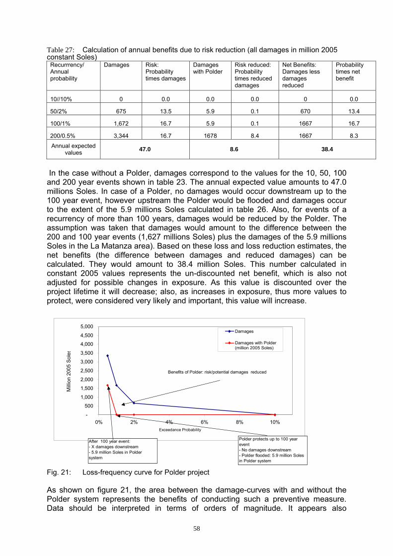
58

Table 27: Calculation of annual benefits due to risk reduction (all damages in million 2005 constant Soles)

Recurrrency/ Annual probability

Damages

Risk: Probability times damages

Damages with Polder

Risk reduced: Probability times reduced damages

Net Benefits: Damages less damages reduced

Probability times net benefit

10//10% 0 0.0 0.0 0.0 0 0.0

50/2% 675 13.5 5.9 0.1 670 13.4

100/1% 1,672 16.7 5.9 0.1 1667 16.7

200/0.5% 3,344 16.7 1678 8.4 1667 8.3

Annual expected values 47.0 8.6 38.4

In the case without a Polder, damages correspond to the values for the 10, 50, 100 and 200 year events shown in table 23. The annual expected value amounts to 47.0 millions Soles. In case of a Polder, no damages would occur downstream up to the 100 year event, however upstream the Polder would be flooded and damages occur to the extent of the 5.9 millions Soles calculated in table 26. Also, for events of a recurrency of more than 100 years, damages would be reduced by the Polder. The assumption was taken that damages would amount to the difference between the 200 and 100 year events (1,627 millions Soles) plus the damages of the 5.9 millions Soles in the La Matanza area). Based on these loss and loss reduction estimates, the net benefits (the difference between damages and reduced damages) can be calculated. They would amount to 38.4 million Soles. This number calculated in constant 2005 values represents the un-discounted net benefit, which is also not adjusted for possible changes in exposure. As this value is discounted over the project lifetime it will decrease; also, as increases in exposure, thus more values to protect, were considered very likely and important, this value will increase.

-

500

1,000

1,500

2,000

2,500

3,000

3,500

4,000

4,500

5,000

0% 2% 4% 6% 8% 10%

Damages

Damages with Polder(million 2005 Soles)

Milli

on 2

005

Sol

es


Polder protects up to 100 year event- No damages downstream- Polder flooded: 5.9 million Soles in Polder system

Benefits of Polder: risk/potential damages reduced

After 100 year event:- X damages downstream- 5.9 million Soles in Polder system

Fig. 21: Loss-frequency curve for Polder project As shown on figure 21, the area between the damage-curves with and without the Polder system represents the benefits of conducting such a preventive measure. Data should be interpreted in terms of orders of magnitude. It appears also

59

necessary to include uncertainty in parameter estimates into the analysis, which will be done at a later stage.

5.4 Calculating economic efficiency In a standard economic project appraisal, benefits are discounted over time and e.g. the net present value calculated (other standard metrics are cost/benefit ratio or internal rate of return). One important issue is the selection of the discount rate, for which values of 0-20% exist in literature and often 12% is used in project practice. Another issue is the selection of the lifetime of a project: the longer a project can be assumed to be in existence, the higher the benefits will be. For the Polder, probably a reasonable value is a 30 year lifetime, as such a flood protection system is exposed to adverse influences and needs to be maintained continually. Also, using the most conservative value on project viability is in accordance with the principle of caution. Discounting benefits over time and subtracting investment costs leads to the net present value as shown in table 26 showing the economic viability analysis done for the Polder system. Table 28: Calculation of costs and benefits of Polder over time NPV, B/C ratio and IRR (Million soles)

Year Calendar Year Costs Benefits Net benefits: benefits-

costs Discounted costs Discounted benefits

Discounted net benefits

1 2005 84 0 -84 84 0 (84) 2 2006 0 39 39 0 35 35 3 2007 0 40 40 0 32 32 4 2008 0 40 40 0 29 29 5 2009 0 41 41 0 26 26 6 2010 0 41 41 0 23 23 7 2011 0 42 42 0 21 21 8 2012 0 43 43 0 19 19 9 2013 0 43 43 0 17 17

10 2014 0 44 44 0 16 16 11 2015 0 45 45 0 14 14 12 2016 0 45 45 0 13 13 13 2017 0 46 46 0 12 12 14 2018 0 47 47 0 11 11 15 2019 0 47 47 0 10 10 16 2020 0 48 48 0 9 9 17 2021 0 49 49 0 8 8 18 2022 0 49 49 0 7 7 19 2023 0 50 50 0 7 7 20 2024 0 51 51 0 6 6 21 2025 0 52 52 0 5 5 22 2026 0 53 53 0 5 5 23 2027 0 53 53 0 4 4 24 2028 0 54 54 0 4 4 25 2029 0 55 55 0 4 4 26 2030 0 56 56 0 3 3 27 2031 0 57 57 0 3 3 28 2032 0 57 57 0 3 3 29 2033 0 58 58 0 2 2 30 2034 0 59 59 0 2 2 31 2035 0 60 60 0 2 2

Sum 84 1464 1380 84 352 268NPV

Note: discount rate used was 12%. In the first year of the project, there would be investment costs of 84 million Soles. There would not be protection against flooding and thus no benefits before the

60

structure was finished. In year 2, there would be no extra costs (as it was assumed that maintenance would be financed by contributions by downstream residents to a fund), but benefits of 39 million Soles (the increase from 38.4 in year 1 to 39.0 million Soles in year 2 is due to assumed increases in exposure by 1.5 % annually as expected increases in exposed population and assets are accounted for. Thus, the benefits in terms of avoided damages to the exposed assets are increasing over time from 38.4 in 2006 to 60 billion Soles in 2035 as more assets and population is put into harms way. Discounting and taking the difference would lead to a net benefit in year 2 of 35 million Soles. Summing net benefits over the years would thus lead to a net present value (NPV) of 268 million Soles over the whole lifetime of the project. Thus net benefits are increasing over time, but on the other hand, due to discounting (i.e. valuing the future less than the present), net discounted net benefits are decreasing over time. 5.4.1 Sensitivity analysis Efficiency calculations rendered a NPV of 268 million Soles, a B/C ratio of 3.8 (352/84 million Soles) and an IRR of 31% (table 29).8 As mentioned, there are a number of uncertainty factors relating to data, future changes and also concerning the appropriate discount rate to use. Thus, it is important to conduct sensitivity analysis to check the effects on results. A number of sensitivity checks were done: Increasing costs ad-hoc by 30%, eg. due to unforeseen price increase in labour or

material inputs. Not taking account of loss of life. Not taking account of indirect effects. Not taking account of increases in exposure.

In all those alternative estimations, a net return with the three efficiency criteria was calculated. However, as benefits were reduced or costs increased, the efficiency decreased, particularly so for the case where no indirect effects were included. Table 29: Alternative results for different assumptions Best estimate Costs: +30% Without loss of

life Without

indirect losses

Without increases in

exposure

NPV (millions) 268 233 259 114 218 B/C ratio 3.8 2.9 3.8 2.2 3.4 IRR 31% 22% 31% 14% 29% Another important issue is the selection of an appropriate discount rate. Varying this rate from 20% to 0%, the efficiency as for example measured by the NPV will change substantially (table 30). Table 30: Dependency of NPV calculations on discount rates

Net present value with discount rate of (million Soles) 20% 15% 12% 10% 5% 0%

NPV 121 192 268 324 612 1350

8 The internal rate of return is defined as the value that discounts the stream of discounted net benefits (the

column on the right) to zero. For example, in excel the IRR can be estimated by selecting the function “IRR” and marking the series of discounted net benefits.

61

A range of 121 to 1350 million Soles for the NPV was computed for the different rates, thus even for a high discount rate of 20%, there would still be a positive social return on this project. 5.4.2 Caveats As discussed throughout this analysis and generally for CBA of risk management measures, there are a number of uncertainties associated with the values calculated. Thus, caution when using the estimates is expressed; the calculations can only be understood as approximations. Uncertainties are inherent in

The recurrency of hazards: estimates are based on two data points only. Incomplete damage assessments: data were not available for all relevant direct

and indirect effects Spatial distribution of damages: as damages partially referred to the whole

department they had to be down-scaled for this report Fragility: fragility curves do not exist, thus in a backward-looking approach they

had to be calculated indirectly Exposure: past dynamics are accounted for, future dynamics are rather unclear

and so far not included. Benefits of risk reduction estimates: the additional benefits of Polder due to

increased irrigation water were not assessed quantitatively due to lack of data Value of life estimates and other adverse health effects: a country-specific value

of 150,000 Soles per fatality was assumed for the value of life lost, other adverse health effects were not included.

Discounting: Different discount rates between 0% and 20% were assumed. In order to do a more comprehensive assessment, some of the following data points would be helpful: More information on the indirect effects. More information on social effects: loss of life and increase in diseases. Update of FEN effects after 2001: Have adverse effects eg in the agricultural

sector prevailed? Distributional impacts: how are different income groups affected, what is the effect

on poverty? Information on future socioeconomic development of basin and region in order to

update potential effects in the future.

62

6 Case Study Semarang, Indonesia

6.1 Introduction Semarang is the capital of the province of Central Java and an important port, industrial and commercial centre. The city currently has a population of 1.3 million with an annual population growth of 1.2%. It comprises an area of 372 km2 with a population density of 3,540 per m2. Population growth has been large at 100% over the last 60 years, a typical phenomenon for Indonesia and many developing countries due to high fertility rates and rural-urban migration. Population expansion has led to increased land demand for residential, industrial and commercial purposes. Furthermore, there are plans to boost Semarang in the future and make it the central hub in eastern Java. This heavy demand on land has partly been met by settlements in hazard prone areas in the northern part of the city (flooding) and in the southern part (landslides). Also, large industrial and commercial areas close to the harbour in these flood-prone areas have been created for the transport and commercial sectors (BGR/GTZ 2004). This case study discusses the efficiency of protecting Semarang against flood and tidal inundation. It first describes the methodology used, the components of a proposed risk management project, followed by the calculation of risk and potential impacts in Semarang. Then, the efficiency of the mitigation options is assessed. Next, some insights derived from an analysis of the institutional context for CBA in Indonesia and Semarang are presented, followed by the conclusion.

6.2 Methodology Various projects have been conducted and are currently under way on assessing the impacts of different hazards in Semarang as well as analysing options for mitigating those. Institutions engaged include the Japan International Corporation Agency (JICA), the World Bank, Asian Development Bank, Dutch development agencies and finally the Bundesanstalt für Geowissenschaften und Rohstoffe (BGR) in collaboration with GTZ through the project “Urban Quality/Mitigation of Geohazards.” This report makes use of these studies, particularly of the work conducted currently by the BGR/GTZ. The following points describe major elements of the methodology employed in the CBA calculations: A forward-looking risk assessment and CBA based on the estimation of risk as a

function of hazard and vulnerability was conducted. The analysis analysed the major hazards flooding during the rainy season as well

as to tidal inundation. Flooding is a probabilistic event, for which hazard and vulnerability are combined

to risk Tidal inundation is a frequent event with city areas continuously and flooded in a

given year. This it can be considered a deterministic event. Losses as assessed in the past are updated for current and future exposure to calculate the damage potential.

The focus was on the city of Semarang and adverse impacts on its population, as well as benefits of risk management measures for local population. Broader regional or national consequences were outside of the scope of this analysis.

63

Impacts assessed in this case study comprise direct and indirect economic damages (table 31). Generally, losses and costs of measures for loss reduction are always deflated, i.e. indicated in constant value terms, here the base year 2005 was chosen. Table 31: Impacts assessed in Semarang case study





Loss of wages, reduced purchasing






AgricultureIndustry

CommerceServices

Environmental Loss of natural habitatsEffects on biodiversity


services

Assets destroyed or damaged:

buildings, roads, machinery, etc.



Losses due to reduced production

Monetary Non-monetary

Use was made of the following data sources for hazard, exposure, fragility, impacts and mitigation options. Table 32: Data sources employed for Semarang case study Step of analysis Source of Information Comment

Hazard BGR/GTZ, JICA

BGR/GTZ has been assessing ground subsidence and landslides, JICA flooding and recurrency periods

Vulnerability Exposure JICA Spatially explicit GIS system currently

under development at BGR/GTZ. JICA exposure values will be checked in the future.

Fragility JICA Fragility functions sampled by means of survey

Risk: Impacts JICA, local sources Only limited and partial information on past events available

Mitigation options JICA Local sources

A number of mitigation options are currently analysed

6.3 Assessing potential impacts and risk 6.3.1 Identifying hazards Semarang is at risk due to tidal inundation (called rob in Bahasa Indonesia) and severe riverine flooding during the rainy season. An aggravating factor for inundation and flooding is the dramatically increased groundwater extraction in the city leading to ground subsidence of on average 4cm/a adding to the naturally occurring soil

64

compression. Another hazard are landslides, which are mainly triggered by heavy rainfalls in the rainy season from January to March. Also indirectly groundwater extraction seems to have an impact on landslide as it affects the pore pressure by means of groundwater level. 6.3.2 Past Impacts Tidal flooding, occurring mainly during high tide, has major impacts in an area of ca. 3,100 ha in the northern part of the city. Some parts are regularly inundated. Most infrastructural installations (roads, bridges, lifeline infrastructure) have been affected in this area around the harbour. Substantial investments are necessary to reinforce and maintain those structures. A large number of residential, industrial and commercial houses are already more than 50 cm below sea level protected by embankments. There are estimates that in 25 year all low-lying areas will be inundated. Some buildings have been abandoned and left to the forces of nature, as the location had continuously been flooded and it had not been economical anymore to raise or otherwise protect those buildings. The train station, 2 meters above sea level when built 120 years ago, has sunk in about 1.5 meters and continually has to be strengthened and protected against water intrusion There is anecdotal evidence on expenses for coping with inundation: a household survey conducted for the JICA study for types of expenditure in 1997, reports losses due to inundation amounting to ca. 11% of average family total expenditure. Furthermore, precipitation during the rainy season causes severe flooding affecting large parts of the city. There is very little information available concerning disastrous flood events in the past. Table 33 lists the information found on the impacts due to the severe floods. Table 33: Effects of flood disasters in Semarang 1973 1990 1993 Affected area (ha) 175 145 200 Fatalities - 47 2 Number of affected houses 420 540 230 Collapsed houses 35 25 60 Damaged houses 120 126 145 Estimated flood damage (billion 2005 Rupiah) 18 23 15

Source: JICA 2000. According to this information, the largest loss so far had been in 1990 which is generally considered a 100 year event. According to this data, losses amounted to ca. 23 billion Rupiah (in 2005 constant values). However, these values seem to considerably underestimate the actual losses that have occurred. In light of the results from the JICA survey conducted for assessing past damages and damage potentials (which will be discussed in this study), the reported values seem very low and to comprise only a tiny fraction of actual impacts. 6.3.3 Flood hazard Tidal flooding correlated with high tide affects the northern part of the city regularly. The following map shows in more detail the area continuously flooded during high tide. Subsidence is a major factor increasing the inundation problem in this area.

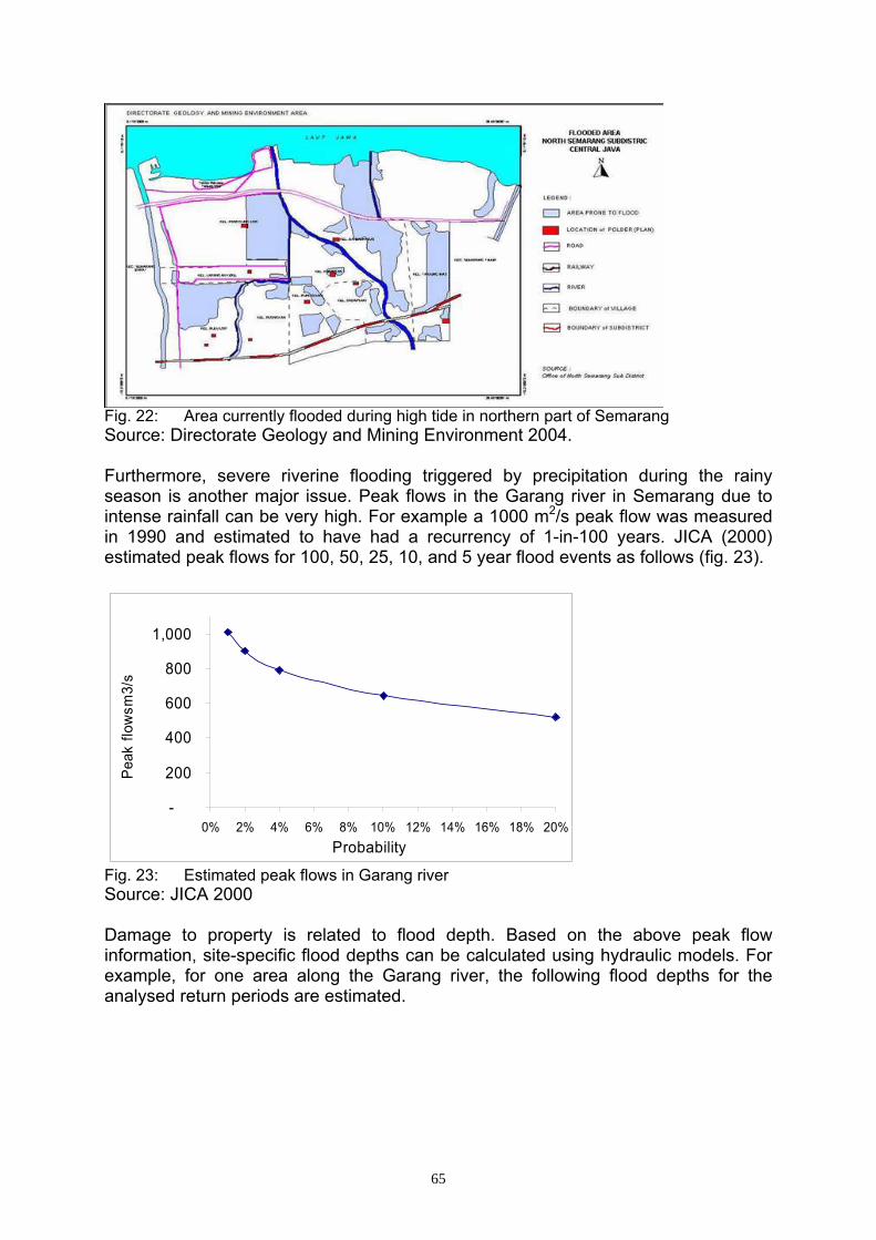
65

Fig. 22: Area currently flooded during high tide in northern part of Semarang Source: Directorate Geology and Mining Environment 2004. Furthermore, severe riverine flooding triggered by precipitation during the rainy season is another major issue. Peak flows in the Garang river in Semarang due to intense rainfall can be very high. For example a 1000 m2/s peak flow was measured in 1990 and estimated to have had a recurrency of 1-in-100 years. JICA (2000) estimated peak flows for 100, 50, 25, 10, and 5 year flood events as follows (fig. 23).

-

200

400

600

800

1,000

0% 2% 4% 6% 8% 10% 12% 14% 16% 18% 20%Probability

Peak

flow

sm3/

s

Fig. 23: Estimated peak flows in Garang river Source: JICA 2000 Damage to property is related to flood depth. Based on the above peak flow information, site-specific flood depths can be calculated using hydraulic models. For example, for one area along the Garang river, the following flood depths for the analysed return periods are estimated.

66

-

0.5

1.0

1.5

2.0

2.5

3.0

0% 2% 4% 6% 8% 10% 12% 14% 16% 18% 20%Exceedance probability

flood

dep

th (m

)

Fig. 24: Water levels due to flooding at one site along the Garang river Source: JICA 2000 The current flood protection by embankments and river gates will generally protect only up to 5 year events with rare events leading to substantial damage. A major factor for the issue of tidal inundation as well for severe flooding is the ground subsidence problem, which has been accelerating over the last few years as a consequence of groundwater extraction. Annual subsidence rates in most affected low-lying areas of Semarang are up to 17 cm per year. While there is a naturally soil compression effect with only a limited effect on subsidence, the major impacts are by way of large scale water extraction through often illegal wells. The increase in groundwater abstraction and water wells over the 20th century has been dramatic. A number of areas are regularly affected by tidal inundation. In the JICA study a survey was conducted to estimate typical levels of inundation depth, annual frequency of inundation and damage in the respective area. Table 34 shows some results of this survey for a selected number of grid cells used for the analysis of flood damages. As can be seen inundation depth may be as high as 70 cm, while annual frequency can be as high as 8 times per year. As a consequence in the areas with highest recurrency, damages were largest, up to 4 billion Rupiah, or as a percentage of exposed assets, 14%. Table 34: Samples from survey on frequently recurring inundation

Number grid cell in JICA study

Exposed values (million Rp in 2005 constant values)

Typical inundation depth (m)

Annual frequency

Total Damage (million Rp in 2005 constant

values)

Damage ratio

1 1,720 0.4 1 13 1% 2 1,253 0.15 3 71 6%

21 27,987 0.4 8 4,030 14% 24 26,384 0.7 2 1,513 6%

Source: JICA 2000.

67

6.3.4 Vulnerability: estimating damages as a function of hazard intensity

6.3.4.1 Exposure For estimating exposure to hazards in Semarang, use was made of JICA data on typical unit values and number of exposed assets as well as BGR/GTZ work on ground subsidence. JICA estimated typical unit values per m2 at risk in the two areas outlined above (table 35). Table 35: Unit values for important elements at risk Category Unit value (Rupiah 2005/m2) Buildings Residential 147,268 Industrial 280,510 Business 280,510 Indoor movable Residential 88,361 Industrial 232,824 Business 385,702 Note: No unit value for public facilities was estimated, damages will be estimated as 46.8% of total asset damages. Data source: JICA 2000. Combining those values with the number of exposed assets allows to calculate total values exposed. Furthermore, when looking into the future, it is necessary to account for increased exposure in a city with strong economic and population dynamics. For the matters of this study, exposure increases were assumed to be in line with forecasted increases in population. Based on a prediction of the Urban Masterplan Document of 2000 of a 1.2% annual population increase, a 90% increase of population from 2005 until 2059 was calculated. The assumption taken here is that economic exposure will increase proportional to this increase in population (table 36). Table 36: Estimated values exposed to flooding 2005-2059 (values in billion constant 2005 Rupiah)

Year Value of assets Indoor Movables Sum Predicted increase compared to 2005

2005 461 500 961 2015 520 563 1,083 13% 2025 585 634 1,220 27% 2035 660 715 1,374 43% 2045 743 805 1,548 61% 2055 837 907 1,744 82% 2059 878 951 1,830 90%

As with the flood losses, inundation losses will increase simply as a result of increased population and economic activity, but also due to the fact that a larger area will be inundated as subsidence worsens. BGR/GTZ has developed scenarios of future ground subsidence. As the following charts show, the area currently just above average sea level (0-0.5 m) will increase in the future, for example as shown here for 2013. This area is currently often under water at high tides.

68

Fig. 25: Elevation levels in 2003 and scenario for 2013 in Semarang Source: BGR/GTZ 2004. Based on the GTZ/BGR estimates, an annual increase in exposed values of 1.5% was estimated. Thus, in total the annual increase in exposure to inundation is calculated at 2.7%, leading to a predicted increase of more than 300% in 2059. Table 37: Estimated values exposed to inundation 2005-2059 (values in billion constant 2005 Rupiah)

Year Assets Indoor Movables Sum Predicted increase compared to 2005

2005 364 334 698 0% 2015 469 430 899 31% 2025 613 563 1176 71% 2035 801 736 1537 124% 2045 1,048 962 2010 192% 2055 1,370 1,258 2628 282% 2059 1,525 1,400 2926 326%

Total values exposed to inundation are forecasted to rise from 698 in 2005 to 2926 billion Rupiah in 2059.

6.3.4.2 Fragility: direct and indirect impacts Fragility is estimated for the probabilistic flood events. For inundation, no fragility curves exist and it is considered a deterministic hazard. Based on a comprehensive flood damage survey conducted in the JICA study estimated fragility curves as the degree of direct and indirect losses as a function of flood level (JICA, 2000). Direct losses:

Buildings (residential, industrial, business) Indoor movable (residential, industrial, business)

Indirect losses: business suspension. Fig. 26 shows those curves for the case of assets. The degree of direct and indirect damage is increasing with increasing flood depth.

69

0%1%2%3%4%5%6%7%8%9%

10%11%12%13%14%15%16%17%18%

- 0.2 0.4 0.6 0.8 1.0 1.2 1.4 1.6 1.8 2.0 2.2 2.4 2.6 2.8 3.0

Flood depth

Residential Industries Business Indirect lossesD

amag

e ra

te

Fig. 26: Fragility functions for direct and indirect flood damages to assets Compared to other functions, such as damage curves of flooding used for example in Australia, the estimates seem to be reasonable. However, one shortcoming is that these curves do not consider the duration of inundation, which is generally acknowledged to be a critical variable as well. Also, no curves were established for public facilities. Total damages were estimated as a fixed fraction of asset damages (46.8%). 6.3.5 Estimating risk: potential damages due to flooding and tidal inundation With that information on hazard and vulnerability, risk due to flooding, a sudden onset hazard, as well as due to tidal inundation, which is a chronic hazard, can be estimated. Given that losses are aggregated over one year periods, tidal inundation can be considered a deterministic event, whereas flooding is a risky event. Tidal inundation: Deterministic occurrence JICA (2000) reports information on annual damages due to tidal inundation for buildings and indoor movables. These values are deflated and updated for increases in exposure. As listed in table 38 total damages amount to ca. 32 billion Rupiah in 2005. Values exposed are estimated at 698 billion Rupiah. Table 38: Annual average losses due to tidal inundation (values in million Rupiah7)

For year 2005 Values exposed Annual losses due to inundation

Direct: Buildings Residential 166 2.0 Industrial 69 0.9 Business 129 1.6 Indoor movable Residential 99 9.6 Industrial 57 5.6 Business 177 12.5 Total in 2005 698 32 *estimated as a fraction of total asset losses. Flooding: Probabilistic event Furthermore, sudden-onset flooding during the rainy season (mostly during the period from January-March), is a serious hazard with a substantial damage potential.

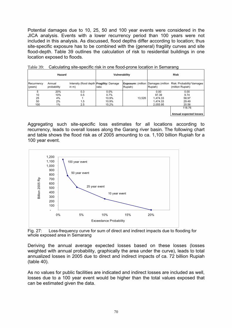
70

Potential damages due to 10, 25, 50 and 100 year events were considered in the JICA analysis. Events with a lower recurrency period than 100 years were not included in this analysis. As discussed, flood depths differ according to location; thus site-specific exposure has to be combined with the (general) fragility curves and site flood-depth. Table 39 outlines the calculation of risk to residential buildings in one location exposed to floods. Table 39: Calculating site-specific risk in one flood-prone location in Semarang

Recurrrency (years)

Annual probability

Intensity (flood depth in m)

Fragility: Damage ratio

Exposure: (million Rupiah)


Risk: Probability*damages (million Rupiah)

5 20% 0.3 0.0% 0.00 0.0010 10% 0.5 0.7% 97.39 9.7425 4% 1 10.9% 1,474.33 58.9750 2% 1.5 10.9% 1,474.33 29.49

100 1% 2.5 15.2% 2,055.95 20.56118.76

Annual expected losses

13,526

RiskHazard Vulnerability

Aggregating such site-specific loss estimates for all locations according to recurrency, leads to overall losses along the Garang river basin. The following chart and table shows the flood risk as of 2005 amounting to ca. 1,100 billion Rupiah for a 100 year event.

-100200300400500600700800900

1,0001,1001,200

0% 5% 10% 15% 20%

Billi

on 2

005

Rp


25 year event

50 year event

100 year event

10 year event

Fig. 27: Loss-frequency curve for sum of direct and indirect impacts due to flooding for whole exposed area in Semarang Deriving the annual average expected losses based on these losses (losses weighted with annual probability, graphically the area under the curve), leads to total annualized losses in 2005 due to direct and indirect impacts of ca. 72 billion Rupiah (table 40). As no values for public facilities are indicated and indirect losses are included as well, losses due to a 100 year event would be higher than the total values exposed that can be estimated given the data.

71

Table 40: Losses due to flooding (billion Rp) in 2005

Direct: Buildings

Values exposed 10 year event

25 year event

50 year event

100 year event

Annual average

losses due to flooding

Residential 95 6 16 24 43 1.7 Industrial 103 5 11 21 31 1.4 Business 90 13 21 30 36 2.8

Indoor movable Residential 198 26 73 108 188 7.8 Industrial 210 29 73 132 200 8.7 Business 265 86 139 193 249 18.3

Public facilities* - 77 157 237 350 19.0 Indirect: business suspension - 10 20 30 45 2.4 Total 961 251 511 775 1,143 72.4 *estimated as fraction of total asset losses. Summary: losses due to floods and inundation Table 41 summarizes the losses to be expected on an annual basis due to flooding and inundation. Losses will increase over time due to increases in exposure and land subsidence. As discussed, asset exposure was predicted to grow by 1.2%; based on experience over the last few years, losses due to land subsidence were estimated to increase by 1.5% per year (GTZ/BGR 2004). Over time, due to increases in exposure and land subsidence, flood and inundation losses will finally increase to ca. 146 billion resp. 137 billion in 2059. Table 41: Losses due to floods and inundation over time (billion Rupiah 2005) Year Annual average losses due

to flooding Annual losses due to

inundation Total losses

2005 72 32 105 2015 82 42 124 2025 92 55 147 2035 104 72 176 2045 117 94 211 2055 132 123 255 2059 146 137 283

6.4 Identification of mitigation and project alternatives The lack of effectively controlling these hazards seriously puts the future development of the city at risk. At the same time, the water provision is at the heart of the problem, as insufficient water is currently provided by the water authorities (only ca. 40% of total water demand), leading to illegal tapping of groundwater, leading again to increased ground subsidence affecting mainly the lower-lying areas of the town. A number of options have been proposed, such as a seaborne dam in front off the harbour and the installation of more drainage pumps (see table 42).

72

Table 42: Options under discussion Project alternative Characteristics Costs (2005 values) Dam protecting harbour Dutch development cooperation

Dam would protect city from seaside inundation, but not riverine flooding

150 billion Rupiah

Installation of more drainage pumps World Bank.

Pumps (to some extent installed) help with flooding and inundation, but do not stop subsidence problem

87 billion Rupiah

Integrated management of flooding and water supply JICA

A: West floodway/Garang River Improvement B: Jatibarang Multipurpose Dam C: Urban drainage system improvement

Total: 437 billion Rupiah • Construction: 337 billion

Rupiah • Operation and

maintenance: 99 billion Rupiah

JICA has proposed an integrated solution for dealing with the flooding and water supply issues. Another idea proposed, but not studied in detail, is to build a water pipeline from the mountainous area in ca. 60 km distance. As more detailed and definite plans have been made for the JICA plans, these options will be discussed in the following. In the JICA study, three components were analysed in detail with a clear perspective for final implementation in mind: A: West floodway/Garang River Improvement

Improvement of West floodway/Garang River including rebuilding existing weir to gate weir. Improved river channel will be able to accommodate floods of up to 25 years recurrency periods (currently 5 years).

B: Jatibarang Multipurpose Dam construction serving multiple functions of flood control: reduction of peak flows during floods from 1010 m3/s to 790

m3/s. water supply hydropower generation with capacity of 1560 kW

C: Urban drainage system improvement: for central Semarang area. Improvement of existing drainage channel and construction of pumping

stations in order to drain storm waters with low recurrency pumps for low land area: lower than 1m+ gravity drainage for higher land area: > 1m+

The main target areas for flood and drainage control as well as the location of the individual project components are shown in figure 28.

73

Fig. 28: Location of target areas for flood and drainage measures and project components in Semarang Source: JICA 2000. In the following analysis, it is assumed that this project would start in 2005. JICA foresees a construction period of 5 years after which only maintenance (for example for the dam) would be necessary. A project lifetime of 50 years is assumed. Thus, the last year considered in this analysis would be 2059. The JICA analysis did not include the subsidence problem, as well no scenarios for increases in exposure of values in the future were considered. These factors will be accounted for in the following analysis. The following cost estimates for the individual project components are listed in the JICA study (table 43). Table 43: Costs for components of JICA project (values in billion RP constant 2005)

Cost West

floodway/Garang River Improvement

Jatibarang Multipurpose Dam

construction

Urban drainage system

improvement Total

Construction 154 68 115 337 Operation and maintenance 33 12 54 99

Total 186 81 170 437 Total project costs (in 2005 constant values) would amount to 437 million Rupiah, of which 337 million Rupiah would arise due to construction and 99 million Rupiah due to operation and maintenance.

74

6.5 Benefits of proposed mitigation project The benefits of the comprehensive JICA package would be: Stopping of ground subsidence (or least very significant slowing-down) as

groundwater extraction would be heavily reduced due to alternative water supply. Better river management will mitigate riverine flooding. It is assumed that potential

damages due to events up to a 100 year flood would be reduced to zero. Damages with a lower recurrency period (i.e. more than 100 years) were not assessed, and would probably cause some damage even with the proposed flood protection measures. However, such events were not considered in this analysis.

Improved drainage will mitigate tidal inundation. It is assumed that potential damages can be reduced by 80% (see JICA 2000).

Benefits in terms of damages avoided will arise only after the construction of the project including its subcomponents has been finished, i.e. in the year 2010. JICA reports that flooding could be completely stopped and tidal inundation impacts reduced by 80%. Thus, for example, in the year 2010, total expected annual benefits would amount to about 107 billion Rupiah (table 44). Table 44: Calculation of benefits due to reducing flooding and tidal inundation in year 2010 Flooding (recurrency)

Damages Risk: Probability times damages

Damages with risk management

Risk reduced: Probability times

Net Benefits: Damages less

Probability times net benefit

5 - 10 270 27 - - 270 27 25 551 22 - - 551 22 50 835 17 - - 835 17 100 1,231 12 - - 1,231 12

Annual expected value 78.1 0.0 78.1InundationRecurrrency: 100% 37 37 7.4 7.4 29.4 29.4 Total 1,268 115 7 7 29 107 In total, the following net benefits would arise 78.1 billion Rupiah due to reduction of flooding, and 29.4 billion Rupiah due to reduction of inundation (80% of inundation impacts).

Costs and benefits need to be discounted over time until the end of the project lifetime in 2059. A standard discount rate of 12% was assumed. Table 45 shows the costs, benefits and net benefits as well as their discounted values as they arise over time. In this analysis, total discounted benefits due to disaster risk management amount to 699 billion Rupiah, while discounted costs add up to 285 billion Rupiah. Thus the NPV would be 414 billion Rupiah and the B/C ratio 2.5. Furthermore, the IRR is calculated at 23%.

75

Table 45: Calculating efficiency of Semarang risk management project Calendar Project year Benefits Costs Net benefits Disc. Benefits Disc. Costs Disc. net benefits

2005 1 0 19 (19) - 19 (19) 2006 2 0 105 (105) - 93 (93) 2007 3 0 118 (118) - 94 (94) 2008 4 0 80 (80) - 57 (57) 2009 5 0 17 (17) - 11 (11) 2010 6 107 2 105 61 1 60 2011 7 117 2 115 59 1 58 2012 8 118 2 117 54 1 53 2013 9 120 2 119 49 1 48 2014 10 123 2 121 44 1 43 2015 11 125 2 123 40 1 39 2016 12 127 2 125 36 1 36 2017 13 129 2 127 33 1 33 2018 14 131 2 129 30 0 30 2019 15 133 2 131 27 0 27 2020 16 136 2 134 25 0 24 2021 17 138 2 136 23 0 22 2022 18 140 2 138 20 0 20 2023 19 143 2 141 19 0 18 2024 20 145 2 143 17 0 17 2025 21 148 2 146 15 0 15 2026 22 151 2 149 14 0 14 2027 23 153 2 151 13 0 12 2028 24 156 2 154 12 0 11 2029 25 159 2 157 10 0 10 2030 26 161 2 159 9 0 9 2031 27 164 2 162 9 0 9 2032 28 167 2 165 8 0 8 2033 29 170 2 168 7 0 7 2034 30 173 2 171 6 0 6 2035 31 176 2 174 6 0 6 2036 32 180 2 178 5 0 5 2037 33 183 2 181 5 0 5 2038 34 186 2 184 4 0 4 2039 35 190 2 188 4 0 4 2040 36 193 2 191 4 0 4 2041 37 197 2 195 3 0 3 2042 38 200 2 198 3 0 3 2043 39 204 2 202 3 0 3 2044 40 208 2 206 3 0 2 2045 41 212 2 210 2 0 2 2046 42 216 2 214 2 0 2 2047 43 220 2 218 2 0 2 2048 44 224 2 222 2 0 2 2049 45 228 2 226 2 0 2 2050 46 232 2 230 1 0 1 2051 47 237 2 235 1 0 1 2052 48 241 2 239 1 0 1 2053 49 246 2 244 1 0 1 2054 50 250 2 248 1 0 1 2055 51 255 2 253 1 0 1 2056 52 260 2 258 1 0 1 2057 53 265 2 263 1 0 1 2058 54 270 2 268 1 0 1 2059 55 275 2 273 1 0 1

Sum 9,081 437 8,644 699 285 414 Benefits Costs Net benefits Disc. Benefits Disc. Costs Disc. net benefits

Sensitivity analysis To account for uncertainty of the estimates, the following alternative scenarios were calculated. Case without increase of exposure: losses and thus benefits would only increase

due to ground subsidence problem, Case without increase of the subsidence problem: losses and thus benefits would

only increase due to increases in exposure, A combined “no exposure and subsidence increase” scenario, i.e. benefits would

be constant over the whole lifetime

76

Table 46: Results for Semarang case study

Best

estimate No exposure

increase No subsidence

increase No exposure and

subsidence increase NPV (billion Rupiah) 414 296 330 257 B/C ratio 2.5 2.0 2.2 1.9 IRR 23% 19% 21% 18%

In all scenarios, the project remained efficient. Thus, in total, given the available data and assumptions used, the analysed integrated JICA project would be efficient in terms of avoidance of damages due to flooding and inundation in Semarang.

77

7 Conclusions Cost-benefit analysis (CBA) is the major decision-supporting tool commonly used for appraising projects. CBA is used to organize, appraise and present the costs and benefits, and inherent tradeoffs of projects taken by public sector authorities and local, regional and central governments and international donor institutions to increase overall societal welfare. Information by means of CBA may help in motivating investments into risk management, which are too infrequently taken today. Benefits in a CBA in the context of disaster risk management are the impacts avoided. There are social, economic and environmental impacts. Furthermore, these can be differentiated into direct and indirect, monetary and non-monetary effects. While a number of reports on CBA in context of natural disasters exists, these reports are generally written for experts with the sufficient resources and a data-rich context. This report focused on a context with less resources and often incomplete data sets and discussed the suitability of CBA for examining the efficiency and benefits of preventive measures and projects. Two different approaches for measuring the net benefits of disaster risk management were outlined: A risk-based forward-looking approach building on a detailed assessment of

hazard, vulnerability (fragility and exposure) finally leading to risk and risk reduced.

An impact-based, backward-looking approach relying on information on past damages.

A number of important principles that should be followed when conducting a CBA were discussed in this study Measurement in terms of risk: the probabilistic nature of events needs to be

accounted for. The focus should not be on singular events. Future impacts and impacts avoided should be calculated, not those in the past. Estimate should be done in current monetary values, past damages need to be

updated with deflators. There is need for discounting benefits and costs over time. The discount rate

chosen has a strongly effects on the efficiency calculation. Clearly delimit area of analysis: within area only count net losses or benefits. Do with-and without analysis. The benefits of risk management are the reduction

in impacts in the case with measures taken compared to the case without. Generally there are large uncertainties, thus estimates of risk and benefits of risk

reduction should be understood only in terms of orders of magnitude. Case studies Two exemplary CBA case studies were conducted calculating the main efficiency criteria B/C ratio, IRR and NPV. In the first case study, the net benefits of a Polder system for purposes of flood protection during El Niño events in Piura, Northern Peru are calculated. The other case study examined the return on an integrated water management and flood protection scheme in Semarang, Indonesia. In both cases, substantial positive returns in terms of the reduction of potential adverse disaster impacts were calculated. In both studies, direct and indirect economic impacts were considered in the analysis. In the case of Piura, also potential social impacts were included.

78

8 References General Benson, C. (1998). The cost of disasters. Development at Risk? Natural Disasters and the

Third World. J. Twigg (ed.). Oxford, Oxford Centre for Disaster Studies, UK National Coordinated Committee for the International Decade for Natural Disaster Reduction (IDNDR): 8-13.

Benson, C. and J. Twigg (2004). 'Measuring mitigation': Methodologies for Assessing Natural Hazard Risks and the Net benefits of Mitigation - A Scoping Study. Dasgupta, A. K. and D. W. Pearce (1978). Cost-Benefit Analysis: Theory and Practice. London, Macmillan.

Burby, R., Ed. (1991). Sharing Environmental Risks. How to control Governments' Losses in Natural Disasters. Boulder, Colorado, Westview Press.

Dedeurwaerdere, A. (1998). Cost-benefit Analysis for Natural Disaster Management - A Case-study in the Phillipines. Brussels, Belgium, CRED.

Dinwiddy, C. and F. Teal (1996). Principles of cost-benefit analysis for developing countries. Cambridge, Cambridge University Press.

ECLAC (2003). Handbook for Estimating the Socio-economic and Environmental Effects of Disasters. ECLAC, Mexico City.

Endres, A., B. Staiger (1995), Nutzen-Kosten-Analyse der Umweltpolitik, in: M. Junkernheinrich, P. Klemmer und G.R. Wagner (eds.), Handbuch zur Umweltökonomie, Analytica, Berlin.

Federal Office for Civil Protection (2003). Katarisk. Disasters and Emergencies in Switzerland. Risk assessment from a civil protection perspective. Bern.

FEMA (1998). Protecting Business Operations: Second Report on Costs and Benefits of Natural Hazard Mitigation. Washington, DC: Federal Emergency Management Agency, August.

FEMA (2001). Benefit-Cost Analysis (BCA) of Hazard Mitigation Projects. Washington. GTZ (2001). Disaster risk management. Working concept. Eschborn. GTZ (2004). Risk analysis - a basis for disaster risk management. Guidelines. Eschborn. Handmer, J. and P.Thompson (1997). ‘Economic Assessment of Disaster Mitigation: A

Summary Guide’. Resource and Environmental Studies 13. Canberra: Centre for Resource and Environmental Studies, Australian National University.

Hanley, N., C. L. Splash (1993). Cost-benefit Analysis and the Environment. Hants, Edward Elgar.

Hecker, G. (1995). A Review of the Disaster-Related Activities of the Asian Development Bank: An Economic Perspective. Disaster Prevention for Sustainable Development: Economic and Policy Issues. Washington DC, World Bank.

IDB (2000). Facing the Challenge of Natural Disasters in Latin America and the Caribbean. An IDB Action Plan. Washington DC, Inter-American Development Bank.

IFRC (2002). World Disasters Report 2002. Geneva, IFRC. Kramer, R. A. (1995). Advantages and Limitations of Benefit-Cost Analysis for Evaluating

Investments in Natural Disaster Mitigation. Disaster Prevention for Sustainable Development: Economic and Policy Issues. M. Munasinghe and C. Clarke. Washington DC, The International Bank for Reconstruction and Development/The World Bank: 61-76.

Mechler, R. (2002). Natural Disaster Risk and Cost-Benefit Analysis. In Kreimer, A, M. Arnold and A.Carlin (eds.). The Future of Disaster Risk: Building Safer Cities. Conference papers. Washington, DC: The World Bank.

Mechler, R. (2004a). Natural Disaster Risk Management and Financing Disaster Losses in Developing Countries. Verlag fuer Versicherungswissenschaft, Karlsruhe.

Mechler, R. (2005). Cost-benefit Analysis of Natural Disaster Risk Management in Developing and Emerging Countries. Long Study. Interim report for GTZ.

Ministery of Agriculture. (2001). Flood and Coastal Defence Project Appriasal Guidance. Overview. London.

OAS (1991). Primer on Natural Hazard Management in Integrated Regional Development Planning. Washington DC, Organization of American States.

OECD (1994). Project and Policy Appraisal: Integrating Economics and Environment. Paris, OECD.

Otero, R. C. and R. Z. Marti (1995). The impacts of natural diasters on developing economies: implications for the international development and disaster community. In M. Munasinghe and C. Clarke (eds.). Disaster Prevention for Sustainable Development: Economic and Policy Issues. Washington DC, World Bank: 11-40.

79

Penning-Rowsell, E., C. Green, P. Thompson, A. Coker, S. Tunstall, C. Richards, D. Parker (1992). The Economics of Coastal Management - A Manual of Benefit Assessment Techniques (The Yellow Manual). London.

ProVention Consortium (2005). Successful disaster prevention in LAC. http://www. proventionconsortium.org/goodpractices/

Queensland Government, Counter Disaster and Rescue Services (2002). Disaster Loss Assessment: Guidelines.

Ray, A. (1984). Cost-Benefit Analysis. Issues and Methodologies. Baltimore, Word Bank. Reutlinger, S. (1970). Techniques for Project Appraisal under Uncertainty. Washington DC,

World Bank. Rose, A. (2004). Economic Principles, Issues, and Research Priorities in Hazard Loss

Estimation. In Y. Okuyama, S. Chang (eds.). Modeling Spatial and Economic Impacts of Disasters. Berlin, Springer: 13-36.

Smyth, A. W., G. Altay, G. Deodatis, M. Erdik, G. Franco, P. Gülkan, H. Kunreuther, H. Luş, E.Mete, N. Seeber, and Ö. Yüzügüllü (2004). Probabilistic Benefit-Cost Analysis for Earthquake Damage Mitigation: Evaluating Measures for Apartment Houses in Turkey, Earthquake Spectra, February.

Szekeres, S. (2000). La consideracion de desastres naturales en la evaluacion de proyectos federales en Mexico. Analisis y recomendaciones. Washington DC, World Bank.

UK Treasury (2003). Green Book: Appraisal and evaluation in central government. London. Van der Veen, a. (2004). Disasters and economic damage: macro, meso and micro

approaches. Disaster Prevention and Management:: An international Journal 13 (4): 274-279.

Venton, C & P. Venton (2004). Disaster preparedness programmes in India. A cost benefit analysis. Humanitarian Practice Network, ODI, London.

Vermeiren, J. et al. (1998). Costs and Benefits of Hazard Mitigation for Building and Infrastructure Development: A case study in small island developing states. Conference of The International Emergency Management Society.

World Bank (1996). Staff Appraisal report: Argentina Flood Project. Washington DC, World Bank.

World Bank (2003). World Bank Development Indicators. Washington DC, World Bank. Peru case study Aquino, A, T. Santoyo (2004). Guia para la formulacion del analisis de riesgo en proyectos

de infraestructure de riego. PDRS-GTZ, Piura, Peru. Consejo transitorio de administracion regional Region Grau (CTAR) (1998), Valuacion de los

danos ocasionados por el Fenómeno El Niño (Periodo de emergencia 1998). Corporación Andino de Foment (2000). Las lecciones de El Niño: Peru 2000. Ex Libris. Ferradas, P. (200). Las aguas del cielo y de la tierra. Predes. INEI (2003). Sistema Estadistico Departamental, Piura: Compendio Estadistico 2002 INEI (2004). Sistema Estadistico Departamental, Piura: Compendio Estadistico 2002-2003. Maniak, U. (2001). Hochwasserschutzkonzept gegen El Niño Ereignisse am Rio Piura.

Braunschweig. Maniak, U. (2004). Prefeasibility study for flood protection in the Rio Piura basin.

Braunschweig. Mechler, R. (2004b). Piura case study. Interim report for GTZ. Silveri, E.C. (1999), El Fenomeno El Niño en Piura 97/98. van der Veen (1999). La causa fundamental de la vulnerabilidad ante El Niño. In: Prom Peru

(1999). Peru & El Niño 1999: Apredndendo de l;a Naturaleza. Prom Peru, Lima. Vasquez, G. R, O.I. Talledo (2003), Diagnostico de la cuenca del Rio Piura con enfoque de

gestion del riesgo. Piura. Indonesia case study BGR/GTZ (2004). Mitigation of geohazards in Indonesia. Bandung. Effendi, A., D. Murdohardono (2003). Project report on fact finding mission visiting Kota

Semarang, DGMAE, Bandung. JICA (2000). The detailed design of flood control, urban drainage and water resources

development in Semarang in the Republic of Indonesia. Mechler (2004c). Semarang case study. Interim report for GTZ.

80

Annex I: TORS for project manager for commissioning and conducting a CBA Background Cost-benefit analysis is an instrument for the evaluation of the net benefits and efficiency of risk management measures. Furthermore, it is useful for demonstrating that preventive natural disaster risk management pays, and may thus motivate investments into risk reducing and risk financing activities. CBA of natural disaster risk management measures can be done for different purposes and different time and resource commitments. The following exemplary tasks should be conducted when producing a CBA. I. Analysis of context and purpose of CBA Determination of the aim and the setting of the study: This involves: Participatory determination of the specific purpose of the analysis: informational

study, preproject appraisal, project appraisal or ex-post evaluation Survey of general context, in which CBA is conducted Determination of involved persons and institution Identification of target group (s) Determination of timing Identification of funding sources

Outcome: clear idea of purpose, target group(s), involved people, timing and funding sources II. Planning the CBA After determining the broader framework of the CBA, the CBA can be planned in more detail. The following issues are of importance: More detailed time and financial plan Securing funding from identified sources Identifying relevant decision processes which should be informed by CBA

Outcome: Time and financial plan Selection of consultant

III. Conducting the CBA After choosing the consultant for the CBA, the CBA can be conducted. Six tasks for conducting a CBA can be identified. 1. Data gathering Available data on hazards, vulnerability and impacts need to be gathered, sources listed and data critically checked. Impacts need to be deflated into constant values. Outcome: Overview over available data sources

81

2. Choosing methodological approach Depending on data availability and purpose of the CBA, the appropriate approach for estimating risk and risk reduction can be chosen: The forward-looking, risk-based approach: A more rigorous framework combining

data on hazard and vulnerability to an estimate of risk and risk reduced Backward-looking, impact-based: A more pragmatic framework relying on past

damages. In this case, less detail is possible and necessary in steps 1 and 2 of the risk analysis.

Outcome: Delineation of planned methodological approach 3. Risk analysis The risk analysis results in a baseline estimate of risk of the exposed population, assets and the environment. This is the basis for analysing the benefits of risk management. The risk analysis needs to be done with regard to the risk management measures to be identified in the later stage of the analysis, ie potential area affected and benefits due to risk management measures. The risk analysis consists of the assessments of hazard, vulnerability and finally risk. Step 1: Hazard analysis In the hazard analysis, the intensity and recurrency of natural hazards affecting a given area will be assessed. This will lead to the identification of the recurrency period of certain event (such as 100 year, 50 year events etc.). Outcome: Hazard curve, which represents the probability of intensity of certain hazards in given area. Step 2: Vulnerability analysis The vulnerability analysis consists of the assessment of Exposure to hazards: Population, assets, environment Fragility of population, assets and environment to natural hazards: Evaluation of resilience?

It is important to look into the future with regard to exposure and fragility and include this into the analysis (possibly by assumptions or scenarios). Outcome: Location and value exposed elements: population, assets, environment fragilities of expose elements possible changes in exposure and fragility

Step 3: Risk analysis and potential impacts In this step hazard (intensity and frequency) and vulnerability (exposure and fragility) assessments are combined.

82

Outcome: Loss-frequency curve: Probability of losses, such as 100 year event will cause losses to the amount of X, 50 year will cause Y. A general concept that should be used is the loss-frequency curve that also allows to calculate expected losses 4. Analysis of risk management measures and associated costs The examined risk management measures need to be described in detail. Outcome: Description of planned risk management measures: the type and location, planned lifetime, and the costs such as

-investment costs, -maintenance costs planned funding sources possibly additional benefits and impacts.

5. Analysis of risk reduction Assessment of the benefits of risk management in terms of reduced and avoided social, economic, environmental impacts. Dynamics should be accounted for, expected benefits may change over time. Also care should be taken of potential positive and negative side benefits Outcome: Modified loss-frequency curve and table with loss reduction due to certain events, eg. 100 year event will be reduced by X as modified loss-frequency curve, 50 year by Y etc. Expected annual benefits due to risk reduction can be calculated 6. Calculation of economic efficiency Calculation of economic efficiency of risk management measures including sensitivity analyses for important model inputs. Outcome: B/C ratio, or/and NPV or/and IRR. Sensitivity analysis

IV. Presentation of methods and findings in a Final Document A final document will document the steps taken, data analysed and the results arrived at. Transparency is key and the document will clearly outline the data and literature sources as well as the assumptions used in the analysis. Outcome: Report with documentation of methodology, assumptions, data used and results.

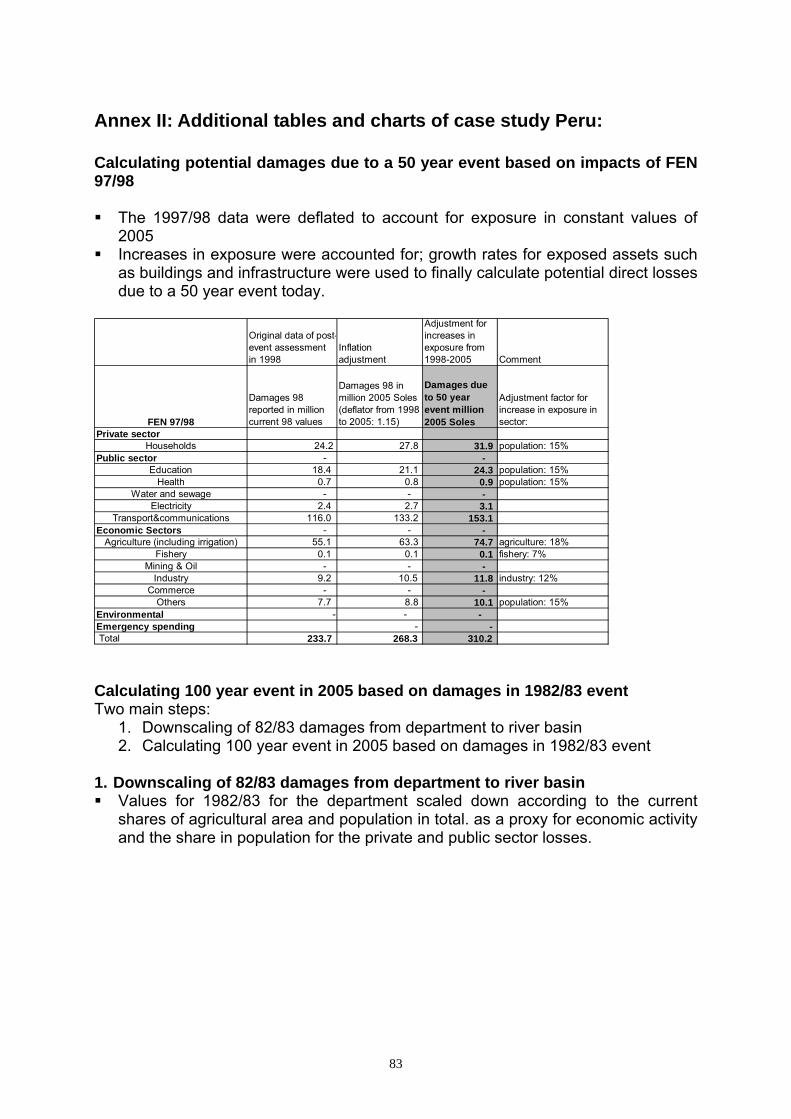
83

Annex II: Additional tables and charts of case study Peru: Calculating potential damages due to a 50 year event based on impacts of FEN 97/98 The 1997/98 data were deflated to account for exposure in constant values of

2005 Increases in exposure were accounted for; growth rates for exposed assets such

as buildings and infrastructure were used to finally calculate potential direct losses due to a 50 year event today.

Original data of post-event assessment in 1998

Inflation adjustment

Adjustment for increases in exposure from 1998-2005 Comment

FEN 97/98

Damages 98 reported in million current 98 values

Damages 98 in million 2005 Soles (deflator from 1998 to 2005: 1.15)

Damages due to 50 year event million 2005 Soles

Adjustment factor for increase in exposure in sector:

Private sectorHouseholds 24.2 27.8 31.9 population: 15%

Public sector - - Education 18.4 21.1 24.3 population: 15%

Health 0.7 0.8 0.9 population: 15%Water and sewage - - -

Electricity 2.4 2.7 3.1 Transport&communications 116.0 133.2 153.1

Economic Sectors - - - Agriculture (including irrigation) 55.1 63.3 74.7 agriculture: 18%

Fishery 0.1 0.1 0.1 fishery: 7%Mining & Oil - - -

Industry 9.2 10.5 11.8 industry: 12%Commerce - - -

Others 7.7 8.8 10.1 population: 15%Environmental - - - Emergency spending - - Total 233.7 268.3 310.2 Calculating 100 year event in 2005 based on damages in 1982/83 event Two main steps:

1. Downscaling of 82/83 damages from department to river basin 2. Calculating 100 year event in 2005 based on damages in 1982/83 event

1. Downscaling of 82/83 damages from department to river basin Values for 1982/83 for the department scaled down according to the current

shares of agricultural area and population in total. as a proxy for economic activity and the share in population for the private and public sector losses.

84

Damages in 1983 (million old Soles)

Damages 82/83 in department (million 2005 new Soles),

deflator from 1983-2005: 0.004396*

Damages 82/83 in middle and lower basin in million 2005 Soles

Share assumed for downscaling in sector

Share assumed for downscaling

Private sectorHouseholds 50,266 221 99 population: 45% 45%

Public sector - - Education 4,760 21 9 population: 45% 45%

Health 940 4 2 population: 45% 45%Water and sewage - - population: 45% 45%

Electricity 9,079 40 18 population: 45% 45%Transport&communications

125,380 551 248 population: 45% 45%Economic Sectors - - -

Agriculture 60,250 265 175 agriculture: 66% 66%Fishery 6,027 26 17 agriculture: 66% 66%

Mining & Oil 178,500 785 518 agriculture: 66% 66%Industry - - -

Commerce - - - Others 50.00 0.22 0 population: 45% 44%

Environmental - - - Emergency spending - - - Sum 435,252 1,913 1,087 In 1985, the sol was replaced by the inti, in 1991, the new sol replaced the inti: 1 new sol=1million intis=1 billion old soles. 2. Calculating 100 year event in 2005 based on damages in 1982/83 event Downscaled damages in constant terms in 1982/83 are increased to account for

increases in exposure, decreased to represent for the fragility reducing effect due to dike increases and

the early warning systems installed. For the fragility reducing effects expert judgment based on the experiences in the

two events was used.

Damages 82/83 in middle and lower basin in

million 2005 Soles

Adjustment for increases in exposure

from 1983-2005Comment

Adjustment for decreases in fragility

from 1983-2005

Damages 82/83 in middle and lower basin in

million 2005 Soles

Damages 100 year event

Adjustment factor for increase in exposure: growth rate in sector

Damages 100 year event in 2005 based on FEN 1982/1983

Private sectorHouseholds 99 144 population: 45% 88

Public sector - - Education 9 14 population: 45% 11

Health 2 3 population: 45% 2Water and sewage - - population: 45%

Electricity 18 26 population: 45% 20Transport&communications

248 360 277Economic Sectors - -

Agriculture 175 231 agriculture: 32% 206Fishery 17 22 fishery: 24% 19

Mining & Oil 518 518 463Industry - - industry: 34%

Commerce - - Others 0.10 0.14 population: 45% 0.1

Environmental - - Emergency spending - -Sum 1,087 1,317 1,087

Cost-benefit Analysis of Natural Disaster Risk … Analysis of Natural Disaster Risk Management in...

Documents

Transcript of Cost-benefit Analysis of Natural Disaster Risk … Analysis of Natural Disaster Risk Management in...