Cost-Benefit Analysis of LEED Silver Certification for New House Residence Hall at Carnegie Mellon University

Civil Systems Investment Planning and Pricing Project

Christopher L Weber Sanath K Kalidas

Department of Civil & Environmental Engineering

Carnegie Mellon University

Fall 2004

- 2 -

Table of Contents Table of Contents ...................................................................................................................................................2 List of Figures ........................................................................................................................................................2 List of Tables..........................................................................................................................................................2 Executive Summary ...............................................................................................................................................3 Acknowledgements ................................................................................................................................................4 Introduction ............................................................................................................................................................5 Background—LEED Certification Objective and Eligibility.................................................................................5 Methodology ..........................................................................................................................................................6

Elicitation procedure .........................................................................................................................................7 Survey Procedures .............................................................................................................................................9

Survey Results ............................................................................................................................................10 Statistical Analysis ..........................................................................................................................................12

Modeling—Costs .................................................................................................................................................13 Modeling-Benefits................................................................................................................................................16 Results ..................................................................................................................................................................19

Result 1:Ranked Net Benefits over 20-year project life…………………………………….…..19 Result 2:Ranked Net Benefits over 40-year project life………………………………………...20 Result 3: Low-end Estimation-Net Benefits over 20-year project life…...……………………..21 Result 4: High-end Estimation-Net Benefits over 40-year project life…...…………………….22 Result 5: Null Expert scenario over 20-year project life………………………………………..23 Result 6: Null Expert scenario over 40-year project life………………………………………..24 Result 7: Student Willingness to pay -Net Benefits over 30-year project life…………………..22

Importance Analysis………………………………………………………………………………..…23 Conclusions…………………………………………………………………………………………...24 Appendix A: New House Benefit Survey.…………………………………………………................28 Appendix B: BestFit distributions used in Analytica Model…………………………………………30 Appedix C: Additional Results…………………………………………………………………..…...31

List of Figures

Figure 1: BestFit regression for Cohon Broader Education benefits…………………..……………..………. ..16 Figure 2: First Costs Model…………………………………………………………………………..………….16 Figure 3: Pdf for Total first costs……………………………………………………….………………….…….16 Figure 4: Present Benefits schematic………………………………………………….………………................18 Figure 5: Student Performance benefits model ……………………………………….………………................18 Figure 6: Publicity benefits model ……………..…………………………………….……………………….…18 Figure 7: Ranked Net Benefits over 20-year project life …………………………...……..………………….…19 Figure 8: Ranked Net Benefits over 40-year project life ……………...……..…………….…………………....20 Figure 9: Low-end Estimation-Net Benefits over 20-year project life……...…………….………………….….21 Figure 10: High-end Estimation-Net Benefits over 40-year project life...……………………………………....22 Figure 11: Null Expert scenario Net Benefits over 20-year project life…………………………………………23 Figure 12: Null Expert scenario Net Benefits over 40-year project life…………………………………………24 Figure 13: Student Willingness to pay -Net Benefits over 30-year project life………………….…………........25 Figure 14: Importance Analysis Results…………………………………………………………………………26

List of Tables

Table 1: Elicitation values ..................................................................................................................................…8 Table 2: Willingness to Pay Survey for Added Benefits of staying in New House at CMU……………………10 Table 3: Stegall Cost estimates and associated modeled distribution.….......................................…………… ..14 Table 4: Ranked Net Benefits over 20-year project life……………….…………………………………..…….19 Table 5: Ranked Net Benefits over 40-year project life ……………………………………………………...…20 Table 6: Low-end Estimation-Net Benefits over 20-year project life ……………………..................................21 Table 7: High-end Estimation-Net Benefits over 40-year project life .……….…………..........…………….….22 Table 8: Null Expert Scenario Net Benefits over 20-year project life………………………………………...…24 Table 9: Null Expert Scenario Net Benefits over 20-year project life………………………………………...…24 Table 10: Student Willingness to pay -Net Benefits over 30-year project life……………...............…………..23

- 3 -

Executive Summary

The objective of this project was to quantify the benefits associated with the decision to pursue LEED (Leadership in Energy and Environmental Design) Silver certification for New House, the latest residence hall built on the Carnegie Mellon University campus. Construction of New House residence hall was completed in August 2003, and the U.S. Green Building Council certified New House as LEED Silver in October 2003. New House is the first LEED certified university residence hall in the U.S. The project assessed and quantified the intangible benefits to the university arising from the LEED Certification and the benefits to the residents of New House through a combination of expert elicitation and surveying. For the purpose of quantification, the benefits were classified into four groups: informal education of the residents of New House, publicity benefits to the university, building performance benefits, and direct student health and performance benefits. A fifth group of benefits was added by two of the experts—internal education and pride amongst students and staff of Carnegie Mellon. The key components of the analysis included the enumeration and quantification of the benefits as well as further modeling of past work quantifying the ‘green premium’ extra cost to create a LEED-certified building. To acquire the information needed for comparison of costs and benefits to the university, interviews were conducted with key decision makers involved in the project. In addition, to derive a direct student benefit, an online survey was conducted with past and current residents to gather their willingness to pay for the benefits of living in New House. After the values were elicited, a probabilistic cost-benefit model was derived using AnalyticaTM statistical modeling software. It was found that the benefits of building New House green far exceeded the costs, and that the net present value of benefits to the university is likely in the millions or even tens of millions of dollars.

- 4 -

Acknowledgements We would like to thank the following people, who helped make this project a success through their time, knowledge, advice, support and patience: Dr. David Dzombak, Professor of Civil and Environmental Engineering, Carnegie Mellon Nathan Stegall, Carnegie Mellon Alumnus and Author of “Cost Implications of LEED Silver Certification for New House, Residence Hall at Carnegie Mellon University”, Senior Honors Research Project, CIT, Carnegie Mellon Kenneth Kimbrough, Vice President, Carnegie Mellon FMS Brad Hochberg, Energy Manager, Carnegie Mellon FMS Peg Hart, New House Project Manager, Carnegie Mellon FMS Tim Michael, New House Owner, Carnegie Mellon Housing Services M. Shernell Smith, New House Housefellow, Carnegie Mellon Housing Services Special thanks to Dr. Jared L Cohon, President, Carnegie Mellon, for his invaluable input and comments, which helped us, gain a better perspective of the benefits to pursue LEED Certification for New House and all new construction on campus.

- 5 -

Introduction Carnegie Mellon University (CMU) is renowned for its pioneering effort in environmental practices. As part of its initiative to promote sustainable design, the university committed in 2001 to LEED (Leadership in Energy and Environmental Design) certification for all newly constructed buildings on campus. This commitment came in the midst of designing New House, the newest residence hall on campus. While Carnegie Mellon already utilized high building performance standards for all buildings on campus prior to the decision to pursue LEED certification for all new projects, achieving LEED Certification distinguishes building projects that have demonstrated a commitment to sustainability by meeting the highest building performance standards. Specifically, LEED Certification is a green building rating system developed by the U.S. Green Building Council, which helps to promote environmentally sustainable building practices across the United States1 (USGBC, 2004). The construction of a LEED certified building can involve considerably more design effort and capital cost than a conventional building. However, when designed correctly, this extra capital cost, often known as the ‘green premium’, can be minimized considerably. Although several studies have attempted to quantify the ‘green premium’ for different projects, relatively few studies have been published which attempt to quantify the benefits of building green, perhaps due to the fact that many of these benefits are difficult to measure and/or intangible in nature. This Cost-Benefit Analysis Project seeks to quantify the benefits and further model the previously studied extra capital costs2 associated with the university’s first LEED Certified building, New House residence hall. Background—LEED Certification Objective and Eligibility For Carnegie Mellon, pursuing LEED Certification achieves several objectives, including establishing recognized leadership in the sustainability and green design sectors as well as qualifying for a growing array of state and local government incentives. The ultimate goal of the LEED process on a national scale is to contribute to a growing green building knowledge base and to promote environmental stewardship in construction around the country. In order to be eligible for the LEED Certification, a proposed building must qualify as a commercial building as defined by standard building codes and be eligible for certification under LEED Version 2.1. Commercial occupancies include but are not limited to: offices, retail and service establishments, institutional buildings (e.g., libraries, schools, museums, churches, etc.), hotels, and residential buildings of four or more habitable stories. A project is a viable candidate for LEED certification if it can meet all prerequisites and achieve a minimum of 26 of the total 69 points. LEED Silver status, which is Carnegie Mellon’s goal for all new buildings, can be added at 33 points, Gold at 39, and LEED Platinum status at 52. There are substantial monetary and societal benefits to building green, although many of these benefits are difficult to easily identify and quantify. These benefits include energy 1 U.S. Green Building Council (USGBC 2004) 2 Stegall. N, Cost Implications of LEED Silver Certification for New House, Residence Hall at Carnegie Mellon University, Senior Honors Research Project, CIT, Carnegie Mellon

- 6 -

savings through reduced electricity, heating, and cooling, building resident productivity gains through increased comfort, reduced environmental footprint, and an increase in societal education and concern for sustainability. Oftentimes, the additional costs of building green are given substantially more attention than these potential benefits, perhaps because the benefits accrue over the course of the life cycle of the building, while the additional costs are capital costs that must be paid upfront. Due to this fundamental time differential in costs and benefits, it is necessary to consider life cycle costing of any green building project. Methodology To perform a benefit-cost analysis, it is necessary to have metrics for both the benefits of a project and the costs of a project. While monetizing both benefits and costs into either a net present value or an equivalent annual value is one option, it is certainly not the only option. Many other methods of comparing benefits and costs exist, such as cost-effectiveness methodologies, multiple-objective models, and decision analysis. When analyzing which method to utilize for this study, several things were taken into account: time restrictions, ease of use and understanding, and availability of data or elicited values for each system. Given the time restrictions of the project over the course of one semester, a complete multiple-objective model seemed unlikely, as serious experimental design would have had to be done to complete such a model. However, because many of the identified benefits for the project are intangible and difficult to monetize, the multiple-criteria model was considered initially. One of the major deciding factor was data availability; the recently-completed report by Stegall2 already detailed all of the first costs associated with building New House LEED-certified in dollar terms, as well as presenting energy modeling that presented yearly energy savings in dollar terms. Although this data likely could have been combined with a multiple-criteria model, the obvious choice was to keep with the previous work and use monetized values to compute a net present benefit value for the project. Before any benefits could be monetized, though, the benefits had to be identified and classified. Through a combination of brainstorming and interviews with campus officials (M. Shernell Smith, Housefellow at New House, Bradley Hochberg, Energy manager for CMU, and Dr. David Dzombak, co-chair of campus Green Practices) four classes of benefits were identified (in addition to the energy benefits already identified by Stegall). These classes were: 1) publicity and external relations benefits from being the first university in the country to build a LEED-accredited dormitory, 2) informal education benefits of the students living in New House learning about environmental issues and sustainability, 3) building performance benefits from the additional commissioning that the building underwent as part of the LEED process, and 4) student performance benefits for the residents of New House due to access to 100% fresh, recycled air and natural lighting. Monetizing these mostly intangible benefits presented a serious problem. One method commonly utilized for monetizing intangible benefits is expert elicitation, where knowledgeable ‘experts’ are asked to estimate the benefit based on past experience, research, and professional observation. Because these identified benefits were not only difficult to monetize, but also extremely uncertain, a probabilistic approach was taken where values were elicited at different probability levels to obtain an empirical distribution for the unknown benefit parameter. A description of the elicitation process follows. This description specifically details the first

- 7 -

elicitation, with Ms. Peg Hart, project manager for New House, though the same procedure was followed for all four elicitations.

Elicitation procedure Upon first meeting with Ms. Hart, the project was introduced, along with the four classes of benefits that had previously been identified. The differences between probabilistic and deterministic analyses were explained, and finally the format of the interview was fully explained before going over an example question to further show what the format would be like. Before beginning the elicitation, Ms. Hart was also given a brief introduction on anchoring and adjustment bias and some of the other cognitive biases that are common in expert elicitation. Literature on cognitive biases is available for further interest34, but for this report, it is be sufficient to say that it was attempted to correct for them. All questions were asked in the following form: “what is your best estimate value for the willingness to pay for (benefit), per year, such that the probability of this benefit being less than Y is X?” where X included values at 0.02, 0.25, 0.5, 0.75, and 0.98. Yearly values were used because all of the benefits were taken to be continuing benefits throughout the life cycle of the building unless otherwise noted by the expert. It was noted and clearly stated that each of the elicited benefit values was to be a yearly, incremental value, meaning a benefit above and beyond what would have been received had New House been built within the tenets of standard Carnegie Mellon construction. To ensure that the concept was completely understood, I often referred to the median value as the “best estimate”, although this is only strictly true for symmetric distributions, and the 2nd and 98th percentiles as the “extreme values” where the expert was 98% sure the real value was below or above these values. Each questioning started with the 98th percentile estimate to avoid anchoring onto the median estimate, then proceeded to 2nd percentile, median, and finally 25th and 75th percentile. As the elicitation went on, the experts got much more comfortable answering the questions, which generally meant they got much more confident as well, which in turn tended to underestimate the real uncertainty in the values. After a total of twenty questions was asked (five probability values for each of four benefit classes) the expert was asked if there were any benefits that CMU received due to the LEED decision that were not included in the four classes that were presented. Although Ms. Hart could not think of any, two of the respondents, Kenneth Kimbrough, Vice President of facilities and Jared Cohon, president of CMU, did present benefit classes that we had previously not considered. Both of these men presented a fifth class of benefits described as ‘broader education’ benefits, which were explained to be the broader informal education and pride benefits to those outside of the New House community (such as other students, faculty, 3 Morgan, M. Granger and Henrion, Max. Uncertainty: A Guide to Dealing with Uncertainty in Quantitative Risk and Policy Analysis. Cambdridge University Press (2001). Cambridge. 4 Hastie, Reid and Dawes, Robyn M. Rational Choice in an Uncertain World. Sage Publications, (2001). London.

- 8 -

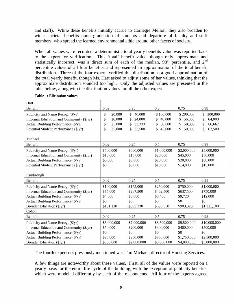
and staff). While these benefits initially accrue to Carnegie Mellon, they also broaden to wider societal benefits upon graduation of students and departure of faculty and staff members, who spread the learned environmental ethic around other facets of society. When all values were recorded, a deterministic total yearly benefits value was reported back to the expert for verification. This ‘total’ benefit value, though only approximate and statistically incorrect, was a direct sum of each of the median, 98th percentile, and 2nd percentile values of all four benefits, and represented an approximation of the total benefit distribution. Three of the four experts verified this distribution as a good approximation of the total yearly benefit, though Ms. Hart asked to adjust some of her values, thinking that the approximate distribution sounded too high. Only the adjusted values are presented in the table below, along with the distribution values for all the other experts. Table 1: Elicitation values

Hart Benefit 0.02 0.25 0.5 0.75 0.98 Publicity and Name Recog. ($/yr) $ 20,000 $ 40,000 $ 100,000 $ 200,000 $ 300,000 Informal Education and Community ($/yr) $ 16,000 $ 24,000 $ 40,000 $ 56,000 $ 64,000 Actual Building Performance ($/yr) $ 25,000 $ 33,333 $ 50,000 $ 58,333 $ 66,667 Potential Student Performance ($/yr) $ 25,000 $ 32,500 $ 45,000 $ 50,000 $ 62,500 Michael Benefit 0.02 0.25 0.5 0.75 0.98 Publicity and Name Recog. ($/yr) $500,000 $600,000 $1,000,000 $2,000,000 $5,000,000 Informal Education and Community ($/yr) $10,000 $15,000 $20,000 $45,000 $50,000 Actual Building Performance ($/yr) $5,000 $8,000 $20,000 $28,000 $30,000 Potential Student Performance ($/yr) $0 $5,000 $10,000 $14,000 $15,000 Kimbrough Benefit 0.02 0.25 0.5 0.75 0.98 Publicity and Name Recog. ($/yr) $100,000 $175,000 $250,000 $750,000 $1,000,000 Informal Education and Community ($/yr) $75,000 $287,500 $462,500 $637,500 $750,000 Actual Building Performance ($/yr) $4,800 $6,600 $8,400 $9,720 $12,000 Actual Building Performance ($/yr) $0 $0 $0 $0 $0 Broader Education ($/yr) $131,110 $393,330 $655,550 $983,325 $1,311,100 Cohon Benefit 0.02 0.25 0.5 0.75 0.98 Publicity and Name Recog. ($/yr) $5,000,000 $7,000,000 $8,500,000 $9,500,000 $10,000,000 Informal Education and Community ($/yr) $50,000 $200,000 $300,000 $400,000 $500,000 Actual Building Performance ($/yr) $0 $0 $0 $0 $0 Actual Building Performance ($/yr) $25,000 $250,000 $750,000 $1,750,000 $2,500,000 Broader Education ($/yr) $500,000 $2,000,000 $3,000,000 $4,000,000 $5,000,000

The fourth expert not previously mentioned was Tim Michael, director of Housing Services. A few things are noteworthy about these values. First, all of the values were reported on a yearly basis for the entire life cycle of the building, with the exception of publicity benefits, which were modeled differently by each of the respondents. All four of the experts agreed

- 9 -

that publicity benefits would be very large in the first year, dropping quickly to zero over a set number of years, which was estimated between two and five for the different experts. One of the experts (Kimbrough) also introduced an increasing model for building performance benefits, claiming that new buildings, regardless of LEED status, rarely have problems, but the difference between New House and a typical non-LEED residence hall would be more pronounced as the building got older. Thus, values were elicited for the real building performance benefits in year 20, the smallest considered building life, and linearly extrapolated to zero in year 1. Linear increase and decrease were used for each of these benefit classes, as there seemed no reason to use a more complex model. Most of the elicited probability distributions spanned at least one order of magnitude, some up to two orders of magnitude, which exhibits the vast uncertainty in these values. Finally, two of the experts declined to estimate on a class of benefits, claiming too great of ignorance on the matter. This is represented by a row of zeroes above.

Survey Procedures It was also desired to obtain information about benefit values directly from the residents of New House, both past residents living in New House during school year 2003-2004, as well as current residents of the dormitory. Ms. Shernell Smith, Housefellow at New House, was instrumental in convincing students to take part in the survey. Upon first meeting with Ms. Shernell Smith, the project was introduced, and a site visit of New House was conducted to gather information about the salient features of the building design and performance, quality of community space, and student amenities. Based on the inputs from the site visit, the direct student benefits were classified into benefits arising from:

a) Forced Air Ventilation System, providing 100% Fresh outside Filtered Air, Individually Temperature-Controlled, To Every Room

b) Energy efficient Lighting and Heat Recovery System c) Substantial access to natural light and strategic location of windows in design d) Space Planning and Architectural Design that promote Community Interaction e) Environmentally-friendly building design

Based on these benefits, a survey questionnaire was prepared to discover the students’ willingness to pay for these benefits of the New House experience. The objective of the survey was explained to Ms. Smith, who facilitated the circulation of the survey questionnaire amongst current and previous year’s residents of New House. All questions were asked in the following form: “New House was designed with a (specific utilities system) providing a corresponding benefit. Did you notice this benefit? If yes, what is the additional money you would be willing to pay in your yearly room fee for this benefit?’ It should be noted that while the expert elicitations used the more vague language of willingness to pay of the University, the students were asked to directly estimate their own willingness to pay, providing additional insight into these highly uncertain values. To provide a realistic scale of additional willingness to pay for respondents to choose from, dollar ranges of $0-5, $5-10, $10-15, $15-20 and $20 and above were assumed. At the end of the survey, the respondents were asked to total their additional willingness to pay values for all benefits and check whether the sum represented their overall willingness to pay for the

- 10 -

complete New House experience. If not, the respondents were asked to select an alternate willingness to pay value from the assumed dollar ranges of $20-40, $40-60, $60-80. Survey Results The sample space of the survey was 150 responses. Out of the 150 respondents, 56 % were current residents of New House, and 44% were past residents. 7% of the total number of respondents were resident assistants. The following table contains the distribution of additional willingness to pay values across the respondents. When put into a simple monte carlo analysis to estimate what the total student willingness to pay was, a mean of $44 per student per year, with a standard deviation of around $15 was obtained. It was assumed for all further analyses that 250 students will live in New House for the remainder of its life. (there are 256 current residents) Table 2: Willingness to Pay Survey for Added Benefits of staying in New House at CMU

Questions Response Criteria

Number of Responses

Response Percent

1) New House was designed with a forced air ventilation system, providing 100% fresh outside air, filtered for air quality, to every room. Did you notice this benefit? Yes 82 55.03% No 69 46.31% Total Number of Responses 149 Number of people who skipped the question 1 2) If you replied yes to 1), how much additional money would you be willing to pay in your yearly room fee for this benefit? $1-$5 24 27.91% $5-$10 22 25.58% $10-$15 15 17.44% $15-$20 15 17.44% $20 and above 20 23.26% Total Number of Responses 86 Number of people who skipped the question 64

3) New House was designed to allow substantial access to natural light with a strategic window design for rooms and lounges. Did you notice this benefit? Yes 109 74.15% No 39 26.53% Total Number of Responses 147 Number of people who skipped the question 3

4) If you replied yes to 3), how much additional money would you be willing to pay in your yearly room fee for this benefit? $1-$5 35 31.53% $5-$10 28 25.23% $10-$15 22 19.82%

- 11 -

$15-$20 15 13.51% $20 and above 15 13.51% Total Number of Responses 111 Number of people who skipped the question 39

5) New House architecture was specifically designed to encourage community interaction through group study rooms and common areas on each floor. Did you notice this benefit? Yes 132 88.00% No 18 12.00% Total Number of Responses 150 Number of people who skipped the question 0

6) If you replied yes to 5), how much additional money would you be willing to pay in your yearly room fee for this benefit? $1-$5 35 26.72% $5-$10 23 17.56% $10-$15 27 20.61% $15-$20 21 16.03% $20 and above 32 24.43% Total Number of Responses 131 Number of people who skipped the question 19

7) The overall design and LEED accreditation of New House made it a very environmentally friendly building, from the use of certified wood products, to environmental friendly building materials, to an extremely efficient heating and cooling system. Were you aware of these environmental efforts? Yes 107 71.81% No 44 29.53% Total Number of Responses 149 Number of people who skipped the question 1

8) If you replied yes to 7), how much additional money would you be willing to pay in your yearly room fee for this benefit? $1-$5 43 40.19% $5-$10 23 21.50% $10-$15 16 14.95% $15-$20 10 9.35% $20 and above 19 17.76% Total Number of Responses 107 Number of people who skipped the question 43

9) Add up your answers to questions 2.4.6 and 8 if applicable. Does their sum represent what you would pay to for the New House experience? In addition to your residence fee? Yes 105 71.43% No 44 29.93% Total Number of Responses 147 Number of people who skipped the question 3

- 12 -

10) If no to 9), what would you estimate as the total amount you would be willing to pay (per year) for the above mentioned benefits of living in New House? $1-$20 22 44.90% $20-$40 12 24.49% $40-$60 5 10.20% $60-$80 10 20.41% Total Number of Responses 49 Number of people who skipped the question 101 Are/were you a resident of Resident Assistant at New House? Yes 138 95.17% No 9 6.21% Total Number of Responses 145 Number of people who skipped the question 5 11) Did you live in New House last year or are you a current resident? Yes 68 45.64% No 83 55.70% Total Number of Responses 149 Number of people who skipped the question 1

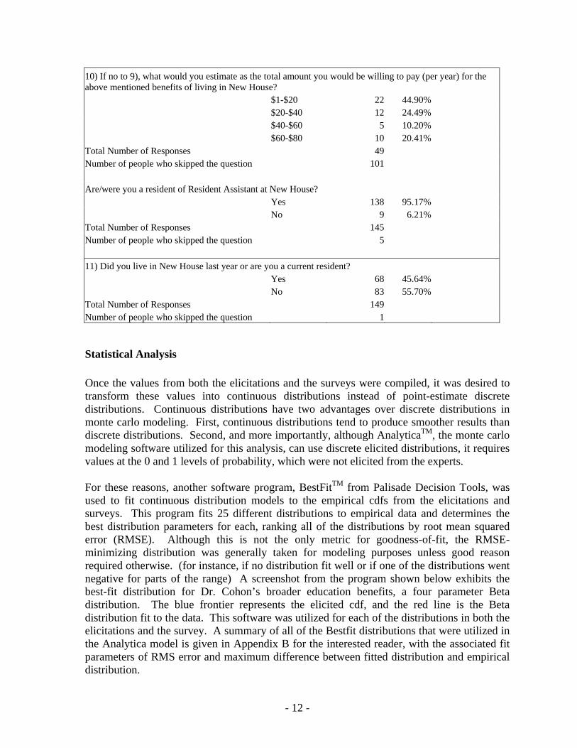
Statistical Analysis Once the values from both the elicitations and the surveys were compiled, it was desired to transform these values into continuous distributions instead of point-estimate discrete distributions. Continuous distributions have two advantages over discrete distributions in monte carlo modeling. First, continuous distributions tend to produce smoother results than discrete distributions. Second, and more importantly, although AnalyticaTM, the monte carlo modeling software utilized for this analysis, can use discrete elicited distributions, it requires values at the 0 and 1 levels of probability, which were not elicited from the experts. For these reasons, another software program, BestFitTM from Palisade Decision Tools, was used to fit continuous distribution models to the empirical cdfs from the elicitations and surveys. This program fits 25 different distributions to empirical data and determines the best distribution parameters for each, ranking all of the distributions by root mean squared error (RMSE). Although this is not the only metric for goodness-of-fit, the RMSE-minimizing distribution was generally taken for modeling purposes unless good reason required otherwise. (for instance, if no distribution fit well or if one of the distributions went negative for parts of the range) A screenshot from the program shown below exhibits the best-fit distribution for Dr. Cohon’s broader education benefits, a four parameter Beta distribution. The blue frontier represents the elicited cdf, and the red line is the Beta distribution fit to the data. This software was utilized for each of the distributions in both the elicitations and the survey. A summary of all of the Bestfit distributions that were utilized in the Analytica model is given in Appendix B for the interested reader, with the associated fit parameters of RMS error and maximum difference between fitted distribution and empirical distribution.

- 13 -

Figure 1: BestFit regression for Cohon Broader Education benefits

Modeling—Costs With all data collected, the next step was to insert all the data into a monte carlo simulation model, which would produce probabilistic outputs, such as net present benefits of the project, from the probabilistic cost and benefit inputs. AnalyticaTM modeling software was used for this purpose. Analytica is a sophisticated modeling environment capable of using both discrete and continuous input distributions for monte carlo analysis of a system. One immediate stumbling block was that all cost data from the previous Stegall report2 (presented in the summary table 2 on the following page, organized by LEED credit obtained) was derived in deterministic, best-estimate terms. Most of the values collected in the Stegall report were estimates from contractors, architects, and construction agencies involved with the construction of New House, and when uncertainty was taken into account, maximum and minimum values were utilized as opposed to probabilistic distributions. Thus, to transform this data into distributions useful in a monte carlo simulation, each specific LEED credit’s uncertainty had to be modeled.

- 14 -

Table 3: Stegall Cost estimates and associated modeled distribution

Extra Cost LEED Credit Low High

Model

SS Prereq. 1: Erosion and Sedimentation Control $0 $0 SS Credit 1: Site Selection $0 $0 SS Credit 4.1: Public Transportation Access $0 $0 SS Credit 4.2: Bicycle Storage and Changing Rooms $0 $0 SS Credit 7.1: Heat Island Reduction, Non-roof $4,120 $4,120 Constant SS Credit 7.2: Heat Island Reduction, Roof $6,750 $13,500 Uniform WE Credit 1.1-1.2: Water Efficient Landscaping $0 $0 EA Prereq. 1: Fundamental Building Systems Commissioning $0 $50,000 Bernoulli EA Prereq. 2: Minimum Energy Performance $0 $0 EA Prereq. 3: CFC Reduction in HVAC&R Equipment $0 $0 EA Credit 1.1-1.2: Optimize Energy Performance $0 $23,000 Normal EA Credit 3: Additional Commissioning $5,827 $15,000 Constant EA Credit 5: Measurement and Verification $16,000 $17,000 Uniform EA Credit 6: Green Power $0 $0 MR Prereq. 1: Storage and Collection of Recyclables $0 $0 MR Credit 2.1-2.2: Construction Waste Management $0 $0 MR Credit 4.1-4.2: Recycled Content $0 $0 MR Credit 5.1-5.2: Local/Regional Materials $0 $0 MR Credit 7: Certified Wood* $4,060 $19,817 Normal,Uniform IEQ Prereq. 1: Minimum IAQ Performance $25,000 $100,000 elicited IEQ Prereq. 2: Environmental Tobacco Smoke Control $0 $0 IEQ Credit 1: CO

2 Monitoring $1,500 $1,500 Constant

IEQ Credit 2: Increased Ventilation Effectiveness $0 $0 IEQ Credit 3.1: IAQ Management, During Construction $21,520 $21,520 Normal IEQ Credit 3.2: IAQ Management, Before Occupancy $0 $0 IEQ Credit 4.1: Low Emitting Adhesives and Sealants $355 $355 Normal IEQ Credit 4.2: Low Emitting Paints $4,190 $4,190 IEQ Credit 4.3: Low Emitting Carpet $0 $0 IEQ Credit 4.4: Low Emitting Composite Wood* $4,060 $4,816 Normal IEQ Credit 5: Indoor Chemical and Pollutant Source Control $0 $0 IEQ Credit 6.1: Controllability of Systems, Perimeter $0 $0 IEQ Credit 7.1: Comply with ASHRAE 55-1992 $9,500 $9,500 Normal IEQ Credit 7.2: Thermal Comfort, Permanent Monitoring $0 $0 IEQ Credit 8.2: Views for 90% of Spaces $0 $0 ID Credit 2: LEED Accredited Professional $0 $0 Cost of Compiling LEED Documentation $25,000 $61,000 Constant Cost of LEED Registration and Certification $1,800 $1,800 Constant Total Extra Cost $129,744 $347,118

- 15 -

These credits were modeled in different ways, depending on how the value was elicited and in what form the value was given from the involved party. (most of the values were taken from interviews with contractors or architecture firms involved in the project) Some of the credits had exact, budget-line values, and thus were modeled as constants. For any value where there was uncertainty in the estimate, but of an unknown quantity, a normal distribution model was used with a standard deviation of 10% of the mean. Although there was no way to verify whether this assumption was accurate or not, the uncertainty in the costs turned out to be dwarfed by the uncertainty in benefits, so this was not perceived as a problem in the overall analysis. For any credits involving hypothetical estimates of amounts that would have spent if internal work had been hired out, these hypothetical prices of internal work were ignored due to a desire to present only real monetary costs to the university. Finally, many of the credits elicited as max-min distributions were modeled as uniform distributions between the max and min values, if the Stegall report indicated that this distribution would be appropriate. A few of the credits required special attention. Energy and Atmosphere (EA) prerequisite 1, the additional cost of commissioning was uncertain not because of cost, but because of the baseline assumption.2 It uncertain whether the building would have been commissioned if LEED accreditation had not been sought. Because of this uncertainty, a Bernoulli variable was introduced with the probability of 0.5 for both baseline commissioning and no baseline commissioning. This seemed reasonable, given the interpretation in Stegall’s report and through personal communication with the author. A similar situation arose for EA credit 1.1-1.2, involving the heat recovery system in New House. Here, however, it seemed that overwhelming evidence presented the case that no heat recovery system would have been utilized had LEED accreditation not been sought; therefore, this cost was modeled as normal around the high estimate. Indoor Environmental Quality (IEQ) prerequisite 1, the requirement for 100% fresh air circulation, was one of the major costs and had a great deal of uncertainty based on two very different estimates.2 To clear up some of the uncertainty, an elicited distribution was used based on Peg Hart’s estimation of the cost, because according to Hart, the other estimate (from the head HVAC engineer on the project) did not properly approximate the value of interest. Finally, an accounting error in CMU’s favor that was included in the Stegall estimates was omitted, and assumed to be actually charged to the university. This assumption was made for the same reason internal work was ignored, because the goal of this analysis was to estimate the actual costs of building New House green, and this cost would have been charged to the University if the error had not occured. A schematic of the cost model in Analytica is shown on the following page in figure 1. Like in the Stegall report, the items were organized based on LEED credit class. The total first costs variable sums all of the extra first costs to produce a range similar to the one given by Stegall. A probability distribution function (pdf) for this total first cost from a 1000 sample run is shown on the following page in figure 2. As can be seen, this variable displays a bimodal behavior due to the random Bernoulli variable for EA Prequisite 1. The overall distribution is tighter than the range presented in Stegall, due to the simplifications and assumptions stated above. The model suggests that the true extra first costs associated with New House is in one of two ranges: either $220,000 to $250,000 or $270,000 to $300,000.

- 16 -

Figure 2: First Costs Model

Figure 3: Pdf for Total first costs

The sensitivity of the model’s assumptions for distribution type was investigated briefly, but as will be seen, uncertainty in benefit values was substantially higher than in cost values, and therefore, changing any of the cost model assumptions had little impact on the net present benefits value for most runs of the model.

- 17 -

Modeling-Benefits A model schematic for net present benefits is shown below as figure 3. This model required substantially more work than the modeling of the first costs, due to a need for combining the elicited expert values shown in Table 1. There are many theories on how best to deal with expert elicitations that yield significantly different values. Two options are typically considered: either the experts should be ranked based on some inherent knowledge about their expertise and weighted together, or not combined at all and examined parametrically to determine the overall effect on the output variable3. (in this case, total net present value of the project) Because there was some limited knowledge about the experts’ knowledge available from their respective professions and comfort with each question, a ranking system was considered first, and is shown on the following page in Table 4. However, due to very large differences in total benefits, it was decided to additionally perform runs of the model using the low-end expert estimations (from Ms. Hart) and the high-end estimations (from Dr. Cohon) parametrically as part of a sensitivity analysis. Runs for Director Michael’s estimations and Vice President Kimbrough’s estimations are also shown in Appendix C. The initial model was constructed using the ranking system to provide easy transition (changing all rankings to 0 or 1) to the parametric analysis.

Figure 4: Present Benefits schematic

The benefits classes were also split into those groups which were modeled as continuous yearly benefits over the entire life cycle of the building and those which changed based on project year, as the former category allowed simple discounting using common annuity

- 18 -

factors while the latter category required year-by-year present value discounting. This explains why in figure 3 above, informal education, energy, student performance, and broader education benefits are all totaled into a dummy variable, yearly benefits, before discounting, while building performance and publicity benefits are each treated separately and plugged directly into the total net present benefit. Table 4: Rankings used in ranked expert model

Rankings Hart Michael

Kimbrough Cohon

Publicity 0.20 0.15 0.25 0.40 Informal Ed 0.15 0.25 0.30 0.30 Building Perform 0.40 0.10 0.50 0.00 Student Perform 0.40 0.40 0.00 0.20 Broader education 0.00 0.00 0.50 0.50

Figure 5: Student Performance benefits model

Figure 6: Publicity benefits model

- 19 -

Two interior nodes are shown above to illustrate the inner workings of the two different categories of benefits. Obviously, the student performance benefits shown in figure 5 were much simpler to model than the publicity benefits shown in figure 6, due to the similarity of timeline. For the publicity benefits, it was necessary first to input the BestFit-derived distributions in year 0, then to linearly discount this distribution through the amount of project years elicited from each expert, followed by a net present value calculation for each year to get all the values in common terms. These were then summed together and added directly to the total net present benefits variable. No matter where the present value calculation was done, it was necessary to consider the appropriate project life and appropriate discount factor for discounting. Both of these values are, by definition, uncertain, but using continuous distributions for them proved impossible because no basis was available for even assuming a distribution for these values. Therefore, it was agreed that parametrically varying these parameters using the built-in index option in AnalyticaTM was the best option. The project life was modeled as varying over 20 years, a very liberal estimate for the life of a new dormitory, to 40 years, which is likely a high estimate for the life of New House, if life is defined as time period without major renovation. For time preference, or discount factor, it was agreed that because CMU is a tax-exempt non-profit organization which yields many such projects each year, the time preference rate should be fairly low compared to a corporation. This rate was varied from essentially 0 (0.0001, so division by zero was not problematic) to 5%. By indexing each of the uncertain present value variables by four values of time preference and three values for project life, a large potential for sensitivity analysis was built into the model. Results The modeling in AnalyticaTM yielded 12 cumulative probabilistic distributions (based on time preference rates and project life) of ranked Net Benefits values for each expert elicitation. The overall ranked Net Benefits (across all expert elicitations) for a project life of 20 and 40 years are presented below as the base cases. For the purpose of highlighting the order of magnitude difference in the Net Benefits and the sensitivity of the model to the different inputs, a low-end scenario is presented using the elicitations from Ms. Hart with a project life of 20 years and a high-end estimation using the elicitations from Dr.Cohon with a project life of 40 years are also presented below. Variation from non-random sampling of experts also needed to be taken into account—it is likely that the sampling of experts was biased in favor of those members of the CMU community who would value these benefits highly. To account for this bias, a model was run using a ‘null expert’ with benefit willingness to pay of 0 ranked as half of the total benefit input. Finally, the benefit values derived from the student survey, added to the fairly certain energy savings, are shown as well. All results are shown in the form of cumulative distribution functions as well as a table showing the calculated distribution statistics. Result 1:Ranked Net Benefits over 20-year project life The overall ranked Net Benefits (across all expert elicitations) for a project life of 20 years, were generated for four time preference rates of 0, 1, 3 and 5%. For the lowest time preference rate of zero, the ranked Net Benefits ranged from $10,740,000 to $76,000,000 with a mean value of $45,480,000 and for the highest time preference rate of 5%, the ranked Net Benefits ranged from $6,605,000 to $47,310,000 with a mean value of $ 28,270,000. The standard deviation indicated that there was a high level of uncertainty with respect to the Net Benefits value across all time preference rates. This was mainly due to the fact that all of the

- 20 -

experts had quite different estimations for the value of the benefits, so when these values were ranked together in the model, the uncertainty grew substantially. Figure 7: Ranked Net Benefits over 20-year project life Table 4: Ranked Net Benefits over 20-year project life 100u 0.01 0.03 0.05 Min 10,740,000 9,673,000 7,932,000 6,605,000 Median 46,350,000 41,840,000 34,460,000 28,820,000 Mean 45,480,000 41,060,000 33,800,000 28,270,000 Max 76,000,000 68,620,000 56,530,000 47,310,000 Std. Dev 13,500,000 12,200,000 10,050,000 8,422,000 Result 2:Ranked Net Benefits over 40-year project life The overall ranked Net Benefits (across all expert elicitations) for a project life of 40 years were similarly generated for each value of time preference. For the lowest time preference rate of zero, the ranked Net Benefits ranged from $21,690,000 to $152,100,000 with a mean value of $91,140,000 and and for the highest time preference rate of 5%, the ranked Net Benefits ranged from $ 9,186,000 to $65,230,000 with a mean value of $ 39,030,000. The high standard deviation again indicated a high level of uncertainty with respect to the Net Benefits value across all time preference rates. Of course, the 40-year project life yielded higher Net Benefits than the 20 year life, because the first costs remained unchanged while the benefits were increased.

- 21 -

Figure 8: Ranked Net Benefits over 40-year project life

Table 5: Ranked Net Benefits over 40-year project life 100u 0.01 0.03 0.05 Min 21,690,000 17,800,000 12,460,000 9,186,000 Median 92,850,000 76,330,000 53,660,000 39,780,000 Mean 91,140,000 74,920,000 52,660,000 39,030,000 Max 152,100,000 125,100,000 87,960,000 65,230,000 Std. Dev 26,980,000 22,190,000 15,620,000 11,600,000 Result 3: Low-end Estimation-Net Benefits, 20-year project life For the low-end expert estimation of Ms. Hart, considered over a project life of 20 years, the net benefits ranged from $608,000 to $ 2,372,000 for a time preference rate of zero with a mean value of $1,432,000, and $ 250,000 to $1,395,000 for a time preference rate of 5% with a mean value of $794,500. The standard deviation of $381,500 for a time preference rate of zero indicated a fair level of uncertainty in the Net Benefits compared to the mean value. Figure 9: Low-end Estimation-Net Benefits over 20-year project life

- 22 -

Table-6: Low-end Estimation-Net Benefits over 20-year project life 100u 0.01 0.03 0.05 Min 608,000 521,100 378,600 270,100 Median 1,433,000 1,272,000 988,800 795,200 Mean 1,432,000 1,268,000 999,200 794,500 Max 2,372,000 2,121,000 1,709,000 1,395,000 Std. Dev 381,500 344,700 284,600 238,900 Result 4: High-end Estimation -Net Benefits over 40-year project life For the high-end expert estimations using Dr. Cohon’s values with a project life of 40 years, the net benefits ranged from $3,210,000 to $ 113,100,000 for a time preference rate of zero with a mean value of $48,590,000 and $ 1,226,000 to $48,470,000 for a time preference rate of 5% with a mean value of $20,740,000. The standard deviation of $30,810,000 for time preference rate of zero indicated that there was an extremely high magnitude of uncertainty with respect to the Net Benefits. This correlated with the fact that Dr.Cohon’s .02-.98 percentile ranges were substantially higher than the other experts, indicating an increased estimation of the uncertainty of his values. Figure 10: High-end Estimation-Net Benefits over 40-year project life Table-7: High-end Estimation-Net Benefits over 40-year project life Table 7: High-end estimation-Net Benefits over 40 year project life 100u 0.01 0.03 0.05 Min 3,210,000 2,593,000 1,745,000 1,226,000 Median 41,440,000 34,040,000 23,880,000 17,660,000 Mean 48,590,000 39,920,000 28,030,000 20,740,000 Max 113,100,000 93,010,000 65,390,000 48,470,000 Std. Dev 30,810,000 25,340,000 17,840,000 13,240,000 Result 5: Null expert ranked at 0.5, 20 yr project life and 40 yr project life To attempt to control any bias that might occur by only sampling from decision-makers who were in favor of the project, a ‘null’ expert was introduced who valued all benefits other than the known energy benefits at $0/yr. This null expert was ranked at 0.5 in the expert rankings, and all of the other rankings were divided by 2 to re-equate the weighted average. Because

- 23 -

the overall model is not linear and is probabilistic in nature, this effect would not necessarily simply cut the net benefit in half, because the discounting factors remain unchanged under these assumptions. The output for both a 20 yr project life and a 40 yr project life are shown below in figures 11 and 12. As can be seen, this new expert dropped the net present benefit of the project substantially, to means of $8 million to $13 million for a 20 yr project life and means of $11 million to $27 million for a 40 yr project life, depending on time preference. These values, while substantially lower than the initial estimates from the experts, may be closer to the true value for net present value, due to several members of the CMU community who likely value the intangible benefits of LEED construction substantially lower than the four experts who were interviewed. Figure 11: Null expert, 20 yr results

Figure 12: Null expert, 40 yr results

- 24 -

Table 8: Null Expert 20 yr project life results 100u 0.01 0.03 0.05 Min 4,057,000 3,641,000 2,957,000 2,437,000 Median 13,590,000 12,250,000 10,060,000 8,386,000 Mean 13,420,000 12,100,000 9,926,000 8,272,000 Max 22,870,000 20,630,000 16,970,000 14,180,000 Std. Dev 3,701,000 3,343,000 2,756,000 2,309,000

Table 9: Null Expert 40 yr project life results

100u 0.01 0.03 0.05 Min 8,357,000 6,829,000 4,734,000 3,449,000 Median 27,420,000 22,510,000 15,770,000 11,640,000 Mean 27,070,000 22,220,000 15,570,000 11,490,000 Max 45,930,000 37,740,000 26,500,000 19,610,000 Std. Dev 7,395,000 6,083,000 4,282,000 3,179,000

Result 7: Student Willingness to Pay (WTP) -Net Benefits over 30-year project life For the student willingness to pay (WTP), considered over the moderate project life of 30 years, the net benefits ranged from - $164,600 to $539,000 for a time preference rate of zero with a mean value of $131,700 and - $ 227,400 to $139,200 for a time preference rate of 5% with a mean value of - $ 59,890. The standard deviation indicated again that there was a good deal of uncertainty with respect to the Net Benefits value across all time preference rates. Thus, when the student-derived benefits, which were substantially lower than the other experts, were considered, the net present benefit was not always positive like in the other scenarios. This is likely due to many factors. First, the students were not asked to estimate the broader benefits like publicity and educational value—their estimates only included direct ones such as comfort and productivity. Second, the students have a much lower comparative income than the professionals estimating the benefits through elicitation. Finally, the students were asked a slightly different question than the experts were, which implied a more direct, out-of-pocket payment rather than a more abstract ‘worth’. Figure 13: Student Willingness to pay -Net Benefits over 30-year project life

- 25 -

Table 10: Student Willingness to pay-Net Benefits over 30-year project life 100u 0.01 0.03 0.05 Min -164,600 -181,100 -207,300 -227,400 Median 127,900 73,180 -7468 -62,330 Mean 131,700 77,240 -4333 -59,890 Max 539,000 424,200 252,400 139,200 Std. Dev 121,600 105,800 82,420 66,920 Other Results: Because of the immense quantity of results, several other model outputs are shown in Appendix C for the interested reader. Further explanation is limited because the outputs are all presented in a similar fashion to the above results. Importance Analysis A convenient way to compare the overall uncertainty in the output variable of a monte carlo analysis is through importance analysis. This statistical test is a measure of uncertainty propagation from input variables to output variables, and the importance essentially ranks how important the uncertainty in the input variable is to the uncertainty in the output variable. This test was performed for the ranked expert model to examine which of the inputs were most important in the overall uncertainty of the net present benefit. A plot showing these values for a number of the important input variables is shown on the following page in figure 14. As can be seen, the overall uncertainty in the output net present value is due to relatively few input variables with high levels of uncertainty. It should be noted that this analysis, because of the way the model was built, could only be run for one value of time preference at a time, so the uncertainty that this variable brings to the overall uncertainty is not shown above. However, the importance rankings did not change substantially when varied across time preference. The highest ranked importance (or most uncertain input variable) is the total broader education benefit, followed by the total student performance benefit, and then the total publicity benefit. This result is not surprising, because whereas the total publicity benefit has the highest per-year values, it only accrues over the first few years of the project, whereas the relatively lower-value benefits of broader education and student performance benefits accrue over the entire life cycle of the building, and so constitute higher portions of the overall uncertainty. Each importance changed based on the project life of the building, but only the publicity benefit changed substantially; this is due to the fact that the changed project life elevated the other benefits in relative share of total benefit. One important observation that can be made from this analysis is that the total first costs represent only a marginal portion of the overall uncertainty in the net present benefit value, especially when compared to the uncertainty of all benefits rather than individual benefit classes.

- 26 -

Importance Analysis for NPB

0

0.2

0.4

0.6

0.8

1

1.2

Total

Broad

er

Total

Stud

ent

Total

Pub

licity

Total

Inf E

d

Total

Ene

rgy

Total

Buil

ding

Total

Firs

t Cos

ts

Category

Impo

rtan

ce 203040

Figure 14: Importance analysis for several inputs to net present benefit

Conclusions Based on the assumptions made in the modeling of the costs and benefits and the final results, it is evident that there is a high level of uncertainty associated with the estimation of benefits and less so in the extra costs associated with the decision to pursue LEED Certification for New House. Though a high level of uncertainty exists in the quantification of these benefits, under nearly all project scenarios the Net Present Benefit value was positive, and on the order of magnitude of millions to tens of millions of dollars. It is thus concluded that the project was a windfall success for the Carnegie Mellon community. The net benefit value using this model, though consistently positive, was heavily dependent on the following parameters:

• the time preference (discounting factor assumed for a non-profit institution like CMU),

• The assumed project life of New House • The expert involved in the elicitation of benefit values (in terms of expertise and

knowledge in LEED Certification costs and benefits) and the student involved in the survey (in terms of awareness of green design practices and the benefits associated with LEED Certification).

While some level of extrapolation may be possible to future LEED projects, this analysis focused on the very unique project at New House, and most, if not all of the costs and benefits will be different in the future. While nearly all of the benefits categories will decrease somewhat with future LEED projects (especially publicity and broader education value), it is also likely that better design and experience will lower the extra first costs associated with LEED accreditation. The leadership that Carnegie Mellon has shown in this project is tremendous, and it is suggested that the practice of LEED construction be continued in the future for all campus construction.

- 27 -

References:

1. N. Stegall, Cost Implications of LEED Silver Certification for New House, Residence Hall at Carnegie Mellon University, Senior Honors Research Project, CIT, Carnegie Mellon, 2004

2. Morgan, M. Granger and Henrion, Max. Uncertainty: A Guide to Dealing with Uncertainty in Quantitative Risk and Policy Analysis.

3. Hastie, Reid and Dawes, Robyn M. Rational Choice in an Uncertain World. London, 2001. Sage Publications.

4. M.H. DeGroot and M.J. Schervish, Probability and Statistics, Addison-Wesley Publications, 3rd Edition, 2002

Websites: 1. www.usgbc.org/LEED/publications.asp (LEED-NC Version 2.1 Rating System) 2. www.palisade.com (BestFitTM, ver 4.5- Distribution fitting software) 3. www.lumina.com (AnalyticaTM, ver 3.0- Decision Modeling Tool)

- 28 -

Appendix-A: New House Benefit Survey Objective of the Survey: Assessment of added benefits of living in New House Thank you in advance for your willingness to participate in this survey. We are conducting a study to attempt to discover the benefits of New House, the first LEED-accredited residence hall in the country, being built in an environmentally friendly manner, specifically to LEED-accredited standards. The following questions will ask you about various benefits you might have noticed due to New House’s environmentally friendly construction. We are interested in whether these benefits were noticed and if so, how much value you would be willing to place on them. For each of the dollar-value questions, please note that the total yearly cost for a room only in on-campus residence halls was $4,964, and any additional willingness to pay for the unique benefits in New House are presumed to be in addition to this fee.

1) New House was designed with a forced air ventilation system, providing 100% fresh outside air, filtered for air quality, to every room. Did you notice this benefit?

2) If you replied yes to 1), how much additional money would you be willing to pay in your yearly room fee for this benefit?

a. $1-$5 b. $5-$10 c. $10-$15 d. $15-$20 e. more than $20

3) New House was designed with an efficient Heat Recovery System along with low-energy intensive lighting fixtures and high performance windows, providing 33% energy savings (by cost) compared to a similar building. Did you notice this benefit?

4) If you replied yes to 3), how much additional money would you be willing to pay in your yearly room fee for this benefit?

a. $1-$5 b. $5-$10 c. $10-$15 d. $15-$20 e. more than $20

5) New House was designed to allow substantial access to natural light with a strategic window design for rooms and lounges. Did you notice this benefit?

6) If you replied yes to 5), how much additional money would you be willing to pay in your yearly room fee for this benefit?

a. $1-$5 b. $5-$10 c. $10-$15 d. $15-$20 e. more than $20

7) New House’s architecture was specifically designed to encourage community interaction through group study rooms and common areas on each floor. Did you notice this benefit?

8) If you replied yes to 7), how much additional money would you be willing to pay for this benefit?

a. $1-$5 b. $5-$10

- 29 -

c. $10-$15 d. $15-$20 e. more than $20

9) The overall design and LEED accreditation of New House made it a very environmentally friendly building, from the use of certified wood products, to environmentally friendly building materials, to an extremely efficient heating and cooling system. Were you aware of these environmental efforts?

10) If yes to 9), how much extra would you be willing to pay to live in such an environmentally friendly residence hall?

a. $1-$5 b. $5-$10 c. $10-$15 d. $15-$20 e. more than $20

11) Add up your answers to questions 2, 4, 6, 8 and 10 if applicable. Does their sum represent what you would pay to for the New House experience, in addition to your residence fee?

a. Yes b. No

12) If no to 11), what would you estimate as the total amount you would be willing to pay (per year) for the abovementioned benefits of living in New House?

a. $0-$20 b. $20-$40 c. $40-$60 d. $60-$80

- 30 -

Appendix-B: Best-Fit distributions used in Analytica Model Hart Publicity—Beta(0.48, 0.84, 19898, 306100) RMS = 4.83 E -6, max dif = 5.2% Hart Inform Ed—Beta(0.57197,0.57197, 15897, 64103), RMS = 3.212E-17 Hart Building—Beta(.45795, 0.29175, 24961, 59302), RMS = 8E-5 Hart Student—Beta(1.0805, 1.1621, 23746, 63390) , RMS = 0.001558, max dif = 6.5% Michael Public—Beta(0.455, 3.424, 499611, 9152495) RMS = 1.28E -5, max dif=5.6% Michael Infed—No adequate fit Michael Build—Beta(0.38132, 0.32955, 4995.5, 29739), RMS = 0.00014, max dif = 6.4% Michael Stud—Uniform(1796,16646), RMS = .00347, max dif = 10.6% KimbroughPublic—No adequate fit Kimbrough Inf Ed—Beta(1.0869, 0.8323, 53909,756248), RMS = 4.56E-5, max dif = 1.2% Kimbrough Build—Beta(1.6511,1.7036, 4213.7, 12455.5), RMS = 0.000222, Max dif=2.2%, 2nd ranked was Uniform, then triangular Kimbrough Broader—Beta(1.0206, 1.1989, 110021, 1361944) RMS = 4.6E-5, Max dif = 1.2% CohonPublic—Beta(1.2060,0.6432, 4685278, 10009708), RMS = 2.52E-6, max dif = 3.2% CohonInfEd—Beta(1.7086, 1.3402, 11238, 517789), RMS = 1.7E-5, max dif = 2.3% Cohon Student—Beta(0.48759, 0.77430, 23929, 2539910), RMS = 0.0001831, Max dif = 5.8% CohonBroader—Uniform(959549, 5057203), RMS = 0.000104, Max dif = 9.0%

- 31 -

Appendix C: Further Results

1. Ranked experts, 30 year project life

2. Ranked experts, 20 year project life, ignoring Broader education benefits, since this benefit could be interpreted as a societal benefit rather than a benefit to CMU

- 32 -

3. Ranked experts, 40 year project life, ignoring broader education benefit

4. Benefits as measured by Tim Michael, 20 yr project life

- 33 -

5. Benefits as measured by Tim Michael, 40 yr project life

6. Benefits as measured by Ken Kimbrough, 20 yr project life

- 34 -

7. Benefits as measured by Ken Kimbrough, 40 yr project life

8. Student survey benefits, plus energy benefits, plus ranked publicity benefits