Cost-based Sharing and Recycling of(Intermediate) Results in Dataflow Programs

Stefan Hagedorn? and Kai-Uwe Sattler

Databases & Information Systems Group, TU Ilmenau,Ilmenau, Germany,

{stefan.hagedorn,kus}@tu-ilmenau.de

Abstract. In data analytics, researchers often work on the same data-sets investigating different aspects and moreover develop their programsin an incremental manner. This opens opportunities to share and recycleresults from previously executed jobs if they contain identical operations,e.g., restructuring, filtering and other kinds of data preparation.In this paper, we present an approach to accelerate processing of suchdataflow programs by materializing and recycling (intermediate) resultsin Apache Spark. We have implemented this idea in our Pig Latin com-piler for Spark called Piglet which transparently supports both, mergingof multiple jobs as well as rewriting jobs to reuse intermediate results.We discuss the opportunities for recycling, present a profiling-based costmodel as well as a decision model to identify potentially beneficial materi-alization points. Finally, we report results of our experimental evaluationshowing the validity of the cost model and the benefit of recycling.

1 Introduction

Today, scalable distributed analytics platforms like Hadoop, Spark or Flink aretypically used together with higher-level languages, either a domain-specificlanguage (DSL) often integrated with a programming language (e.g. Scala orPython) or dedicated high-level dataflow languages such as Pig Latin or Jaqlwhich can be extended by UDFs. Particularly, the latter ones offer the advan-tage of allowing to write complex analytical pipelines in an easy and incrementalmanner. Furthermore, this interactive and incremental formulation is also sup-ported by notebook-like interfaces such as Jupyter or Zeppelin.

For discussing the opportunities for sharing and recycling intermediate re-sults of dataflow programs in Apache Spark we consider the following exemplifieduse case: A (small) group of data scientists has to analyze several datasets con-taining sensor data from weather and environmental observation stations. Thesedatasets contain spatio-temporal data but also metadata describing e.g. sensors.By analyzing this data, models are constructed to represent phenomena whichcan be used for forecasting, classification etc. Main tasks in this process are

? This work was partially funded by the German Research Foundation (DFG) undergrant no. SA782/22.

2

integrating and preparing data (e.g. cleaning, transformation, and reduction),selecting relevant subsets (e.g. by time or region of interest), and applying ma-chine learning and other analytical operations. Typically, this follows a ratherincremental and explorative approach where the dataflow jobs are specified andexecuted step by step to inspect and validate results, test different parameters,and decide about subsequent steps to add further necessary operators. Further-more, multiple scientists might use the same datasets in parallel or simply runmultiple jobs to analyze different aspects. Based on these assumptions, thereexist two obvious opportunities for sharing work:

merge: Merge a batch of submitted dataflow programs into a single job so thatcommon parts are executed only once.

materialization: Explicitly (by user) or implicitly (i.e. automatically) insertsave/load actions to recycle intermediate results across jobs, similar to ma-terialized views.

Recycling results is especially useful when computation power is expensive orlimited, but storage is cheap and available to a large extent. This is often thecase for rented cluster resources on cloud providers like Amazon, Google, orMicrosoft Azure. For example, an Amazon Elastic MapReduce cluster has aper-hour pricing of around $ 2 (c4.8xlarge, Region Frankfurt) but storage iscurrently only $ 0.024 per GB (S3, Region Frankfurt). If the execution timesof the jobs running on such clusters can be reduced significantly, users couldsave a considerable amount of money. Inspired by the concept of materializedviews and adaptive indexing, we present in this paper an approach on mate-rializing and recycling (intermediate) results in Apache Spark-based dataflowprograms. The goal of our work is a transparent materialization and reuse of in-termediate results to unburden the data scientist from decisions about costs andbenefits of materializing results, aggregations, and potentially also indexes. Forthis purpose, we propose a cost-based decision model which relies on profilinginformation obtained by instrumenting the Spark1 runtime environment.

The contribution of our work is twofold: (1) We present and evaluate strate-gies for transparently materializing and reusing intermediate results of dataflowprograms for platforms like Spark. (2) We present a cost and decision modelfor materialization points leveraging platform features and code injection forruntime profiling.

2 Related Work

Caching and reusing intermediate query results has been extensively studiedfor relational databases and data warehouses. Selecting partial results, or viewsrespectively, for materialization [4, 7] as well as rewriting queries using theseviews [6] are two closely related problems that are used in database systems toimprove query response time.

1 https://spark.apache.org/

3

Early works on reusing materialized views (or derived relations) were done byLarson and Yang in [9, 18]. Other research results on the view-matching prob-lems for SQL queries were published in [1] or [15]. In [11] the Hawc architectureis introduced that extends the logical optimizer of an SQL system and considersthe query history in order to decide which intermediate result may be worthmaterializing to speed up further executions – even if this would create a moreexpensive plan which, however, is executed only once. A related problem is au-tomatic index tuning which has been studied extensively [8, 12, 13, 16]. Here,recommenders analyze the given workload and underlying data and recommendto or autonomously create and drop indexes.

For Hadoop MapReduce the MRShare framework [10] merges a batch of jobsinto a new batch of jobs so that groups of jobs can share scans over input filesand the Map output. This is similar to our merging strategy described earlier.Other projects such as ReStore [5], PigReuse [2], or [17] are similar to MRSharein the sense that they all merge a batch of scripts into a single plan or share theintermediate results after a map phase. In PigReuse, the optimization goal isto minimize the number of operators and the number of generated MapReducejobs - but they do not analyze the total cost of the generated plans.

For Spark several additional frameworks were created to support data ana-lysts with their tasks. KeystoneML [14] is able to identify expensive operationsin machine learning pipelines on Big Data platforms like Apache Spark. Theyemploy a cost model using cluster costs (such as network bandwidth, CPU speed,etc.) and operator costs to estimate total execution costs. From this physical op-erators for a logical plan are chosen and materialization points are determined.RDDShare [3] is also based on Spark and simply identifies common operators ina batch of Spark programs and merges them into a single program.

Our work differs from the mentioned approaches in a way that they eitheronly focus on merging a batch of submitted scripts into a single job or they donot use a cost model for their algorithms. Furthermore, most related work isbased on Hadoop MapReduce, except KeystoneML and RDDShare, which dif-fers significantly from Spark’s characteristics. However, KeystoneML focuses onchoosing the best physical implementation of a logical operator and RDDShareonly tries to merge a batch of scripts without reusing intermediate results overdifferent runs.

3 Architecture overview

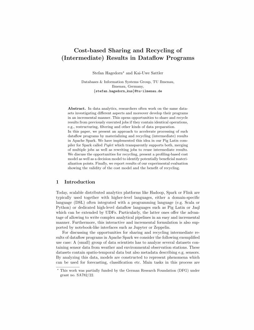
Figure 1 shows the general architecture overview of our approach. Independentlyfrom the used language (Pig Latin, Scala, Pyhton) and platform (Spark, Flink,Hadoop MapReduce), a dataflow program can be represented as a directedacyclic graph (DAG), where operators are the nodes and the directed edgesare the links between these nodes that represent the dataflow. An optimizercomponent receives the DAG for the current job and after applying general rule-based optimizations, the DAG will be modified for recycling. We employ a cachethat will store the materialized results. Ideally, the cache should have access to

4

clusterPa

rser

cache

s 𝜋

ss

⋈ 𝜋

𝜎𝛾s

𝜋

𝜎

𝜋

⋈

𝛾

T

T

T

#1

#1

#2

gloabl operator graph

op

tim

izer

job compile time executiontime

1 2 3 40

Fig. 1. Architecture overview: (0) Transform script to DAG, (1) Insert LOAD for existingdata, (2) Insert STORE (based on statistics), (3) code instrumentation for profiling, (4)execute as Spark job.

HDFS for persistent storage. If materialized data exists for a part of the currentDAG, we first will replace that part with a LOAD operator that reads the cacheddata. In the next step, the global operator graph (see Section 4.3) that storesprofiling information is checked to determine if operators of the current DAGshould be materialized and respective STORE operators are inserted. After that,we insert profiling operators to collect runtime statistics of the operators in thegraph. During execution on a cluster, those operators will send information tothe optimizer which will update its statistics. If intermediate results are to bematerialized, those will be written to the cache by the inserted STORE operators.

We implemented the described cost-based decision model and profiler intoour Piglet project: a parser and code generator from Pig Latin to Spark andother platforms. The code including the implementation of the cost model isavailable at our GitHub repository2. However, we would like to emphasize thatthe model described in this paper is neither restricted to Piglet nor Spark andcould easily be adopted into other platforms. The details of the decision modelthat uses the information in the global operator graph as well as the cache willbe explained in more detail in the next sections.

4 A Cost-based Decision Model

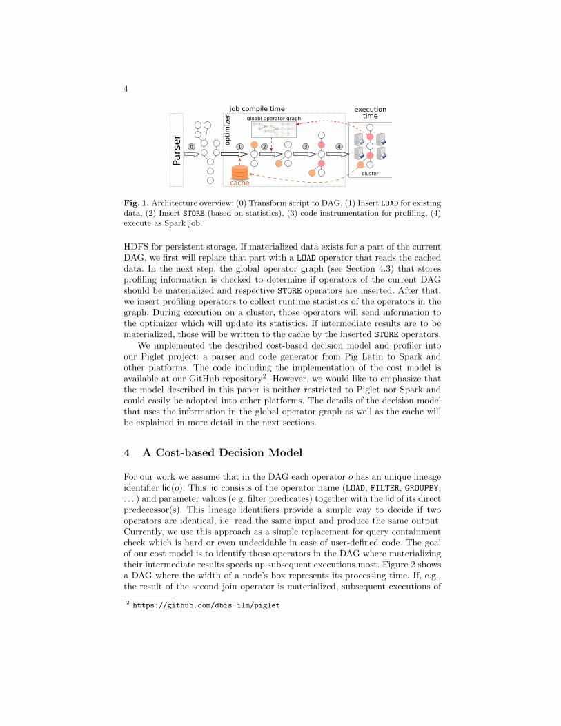
For our work we assume that in the DAG each operator o has an unique lineageidentifier lid(o). This lid consists of the operator name (LOAD, FILTER, GROUPBY,. . . ) and parameter values (e.g. filter predicates) together with the lid of its directpredecessor(s). This lineage identifiers provide a simple way to decide if twooperators are identical, i.e. read the same input and produce the same output.Currently, we use this approach as a simple replacement for query containmentcheck which is hard or even undecidable in case of user-defined code. The goalof our cost model is to identify those operators in the DAG where materializingtheir intermediate results speeds up subsequent executions most. Figure 2 showsa DAG where the width of a node’s box represents its processing time. If, e.g.,the result of the second join operator is materialized, subsequent executions of

2 https://github.com/dbis-ilm/piglet

5

scan

scanscan

𝜋 𝜋⋈⋈𝜎

𝛾

scan 𝜋𝛾texec

𝜋

benefitcache

Fig. 2. Runtime difference for loading materialized result.

dataflow programs that also contain this part in their respective DAG will benefitby only having to load the already present result from disk. This leads to twobasic questions that need to be answered:

(1) If multiple materialized results are applicable for reuse in a job, which ofthem should be loaded?

(2) The intermediate result of which operators in the current job are worthmaterializing so that a subsequent execution will benefit most?

In order to support these decisions, our model introduces materialization points,for which the benefits are calculated.

4.1 Materialization Point

A materialization point M is a logical marker in a DAG denoting a positionfor the decision model to write or load the materialized results. Here, we dis-tinguish between candidate materialization points and materialization points.Candidate materialization points are those potential places in a DAG, where theintermediate result should either be materialized or could be loaded from stor-age. We denote the (candidate) materialization point representing the outputof operator oi by Mi, meaning that Mi is an alias for the output of operatoroi in the optimizer component. Every non-sink operator can be regarded as acandidate materialization point. Obviously, one cannot achieve any benefit frommaterializing the result of a source operator and thus, these materializationpoints need not be considered. We denote the set of all materialization pointsM1,M2, . . . ,Mn which are currently kept in the cache as the materializationconfiguration M = {M1,M2, . . . ,Mn}.

The decision model has to determine if the result of the respective opera-tor is worth materializing or already materialized results can be loaded. Thus,materialization points are always a subset of these candidates.

4.2 Benefit

The decisions are based on the benefit regarding the execution time of the com-plete job with the main goal to minimize the overall execution time. Hence, thebenefit is the amount of time saved when intermediate results can be loaded

6

instead of executing the complete job, as depicted in Figure 2. Alternatively,one can also regard the benefit as the amount of money saved by needing to rentfewer machines in a public cloud.

To calculate the benefit, the decision model is based on the actual costs ofoperators which are measured during execution of a job. For an operator oiuniquely identified by its lid(oi) the following statistics are collected:

– cardinality card(oi): Number of result tuples of oi.– tuple width width(oi): The average number of bytes per result tuple of oi.– execution time texec(oi): Duration it takes the operator to completely pro-

cess its input data.

The benefit of a materialization point Mi can be expressed as in Equation (1).

tbenefit(Mi) = ttotal(Mi)− tread(Mi) (1)

ttotal(Mi) =∑

o∈prefix(Mi)

texec(o) (2)

ttotal(Mi) denotes the cumulative execution time of operators in the prefix of oifrom the source to Mi and tread(Mi) is the time required to read the materializeddata of Mi. If the prefix of Mi does not contain a join (or cross, etc.) ttotal(Mi)can be calculated as in Equation (2). If the prefix of Mi does contain a join(or similar) operator j, with k1(j), . . . , kn(j) as the direct inputs to j, only thelongest (concerning execution time) of those branches is considered:

ttotal(Mi) = max{ttotal(k1(j)), . . . , ttotal(kn(j))} +∑

o∈prefix(Mi)∧o/∈prefix(j)

texec(o)(3)

This means to take the maximum time of all input branches of the join operatorand add the execution times of all other operators in the prefix of Mi which arenot part of the join input, i.e. are located between j and oi. The time to readthe materialized result of Mi is calculated as:

tread(Mi) =card(oi) · width(oi)

bps(4)

The factor bps stands for the number of bytes that can be read per second anddepends on the cluster setup as well as the underlying hardware and thus, is aninstallation-specific calibration factor.

4.3 Global Operator Graph

The benefit of each candidate materialization point is estimated based on ex-ecution of multiple jobs containing the corresponding operator instances. Forthis purpose, the statistics are maintained in a global operators graph, a DAGthat was created by merging the DAGs of all ever submitted jobs. The graph ispersistently stored and, therefore, available across multiple jobs.

7

#runs = 4s 𝜋

ss

⋈ 𝜋

𝜎𝛾s

𝜋

𝜎

𝜋

⋈

𝛾

T

T

T

#1

#1

#2

|𝜎|t𝜎

T

w𝜎

M1

M2

Fig. 3. The global operator graph for four jobs. Stored information on nodes and edgesis exemplarily shown for a single operator node.

With each operator instance, identified by its lid, the collected runtime statis-tics are associated while with each edge its frequency of occurrence in all exe-cuted jobs is stored. Additionally, the global operator graph also contains thematerialization points, i.e., statistics about the already executed operators andmaterialized results. Figure 3 shows an example of such a global operator graphfor four jobs J1 (solid red edges), J2 (dashed blue), J3 (dotted green), and J4(dashed purple)3.

After the execution of a job finished and all statistics (runtimes and resultsizes of the operators) have been collected (cf. Section 5), they are added tothe respective nodes in the graph. If the operator is executed for the first time,no statistics are present for this operator and the collected values are simplyadded to the node in the graph. On the other hand, if the operator was alreadyexecuted before as part of another job, present statistics are merged with thenewly collected ones by averaging them.

The graph serves as input for the decision model and is used to calculate thebenefit based on the statistics and materialization points.

4.4 Decision Model

The decision model is used to answer the two question posed in the beginningof this section.

Loading Existing Materialized Data Answering the first question is straight-forward. From the list of candidate materialization points for a given job, onlythose are selected for which materialized results are present. Then, from thesecandidates, the one materialization point that will result in the highest benefit ischosen to achieve the greatest speedup. If the job contains multiple paths, whichare then combined in a join (or similar), selection of multiple materializationpoint, one for each path, is possible.

Materializing Intermediate Results The decision model has three dimen-sions to consider when choosing a materialization point to actually write topersistent storage.

3 In reality, in the model there is only one edge between the nodes. The multiple edgesare just for illustrating the different jobs.

8

(1) Which candidate materialization points should be selected for further inves-tigation?

(2) From the list of candidate materialization points resulting from (1), whichof those should be materialized?

(3) If the persistent storage is limited in space, decide which existing materi-alized result has to be deleted. Note, that due to space limitations, we donot consider the dimension of cache eviction strategies here and assume aninfinite cache.

Selection of Candidate Materialization Points. Obviously a sink operator is nota candidate for materialization as the result is either written to persistent stor-age anyway or printed to screen. In the latter case, the materialization pointbefore the that sink operator would be one whose result could be re-used by an-other job. A source operator will only read data from storage and pass it to thenext operator without modification. Hence, materializing the output of a sourceoperator will write the same data back to disk and no benefit can be gained fromthis. Therefore, subsequent operations only need to consider candidate materi-alization points that do not belong to a source or sink operator.

Ranking Materialization Points. To decide which materialization point to reallymaterialize, different strategies exist, which might be suitable for different usecases:

– latest: A naıve but intuitive strategy for selecting a materialization pointis to always choose the last possible one. This is the one materialization pointthat is closest to a sink operator. If a job contains n sinks, the materializationpoint before each sink is selected, which means to write n intermediate results.This is a simple caching strategy and might work well during the incrementaldevelopment of scripts, described earlier. However, this bears the “risk” thatthe materialized result will not be needed again, e.g., if subsequently executedscripts are not the next step of the incremental development, but branch offat another operator so that an earlier materialization point would have been abetter choice. Furthermore, the last materialization point may only bring a small(or even no) benefit for reusing.– maxbenefit: Therefore, another option is to choose that one materializationpoint with the highest benefit. Compared to the previous strategy, where thelast one is selected, it is guaranteed to bring the best possible benefit when theresult is needed again. Like in the previous strategy, if the result is not neededagain, materialization was pointless.– markov: Thus, selection of the materialization points should consider theprobability for reuse – for which a Markov chain can be applied. In fact, weshould regard this as a two dimensional (probabilities and benefits) optimiza-tion problem to maximize the benefit as well as the probability for reuse of theselected materialization points. This optimization problem is known as the Sky-line or Pareto efficiency. The result of this optimization problem are all pointswhere there exists no other point with both a higher benefit and higher prob-ability. All points in the Pareto front mark materialization points with either

9

a high probability and/or high benefit, thus being worth materializing. If onlyone materialization point should be selected, it has to be chosen from the Paretofront. For this, the probability of re-occurrence of a materialization point can beconsidered as the weight for the benefit, so that the materialization point withthe highest product of probability and benefit should be selected:

{Mi ∈M | @Mj ∈M, i 6= j :

Ptotal(Mj) ∗ tbenefit(Mj) > Ptotal(Mi) ∗ tbenefit(Mi)}(5)

If this set contains multiple elements, one can be chosen arbitrarily or userspecified weights can be applied to express a favor of one dimension over theother. Ptotal(oi) denotes the minimum probability found on the path in theDAG from the source operators to oi:

Ptotal(oi) = min{Pok,ol |ok, ol ∈ prefix(oi), ok → ol} (6)

where ok → ol means that ol is a direct successor of ok in the DAG. Pok,ol

describes the probability that ok will be followed by operator ol and can becalculated in different ways. One approach is to put the frequency into relationof the total number of executions, with respect to some time window W. Theprobability Pok,ol then would be as in Equation (7)

Pok,ol =fWok,ol

min(W, runs)(7) Pok,ol =

fWok,ol

deg+W(ok)(8)

A second approach is to put the frequency in relation to the possible other oper-ators that follow ok, as shown in Equation (8). Here, fW

ok,olis the plain frequency

count for the transition stored on the edges, that lie within the considered win-dow W, runs is the total number of jobs that are executed by the system, anddeg+W(ok) is the outdegree of a node ok.

5 Profiling Dataflow Programs

Result Size. Unlike traditional DBMS, in the Big Data field one often works withplain text files (log files, csv, . . . ) and no central data management system thathas access to detailed statistics. Thus, in order to gain the desired information,there are two options: (1) The optimizer is started separately to analyze theinput file and create a profile. Before executing a job, the optimizer then triesto come to a decision based on the statistics and selectivity estimations of theinvolved operators. (2) The job is instrumented with code that collects the nec-essary statistics during execution and the runtime or execution platform has tobe extended by such an optimizer that manages and utilizes the collected data.The first approach is more or less what traditional DBMS do and is currentlyalso being implemented in Apache Spark for Spark SQL. However, the secondapproach has the advantage that execution time is measured as well as the resultsize, instead of relying on estimations that are based on assumptions. In our eval-uation we will show that the instrumentation does not incur in any significant

10

overhead. To determine the total number of bytes in the result of an operator,and thus the size of the materialization point, we use Spark’s SizeEstimator

that estimates the number of bytes for a given object. We sample the resultof the operator and pass each result tuple individually into the estimator. Theinformation for each partition is accumulated using Spark’s accumulator mech-anism and send to the optimizer. From the received information the optimizecan calculate the average tuple size as well as the total number of tuples in theresult.

Execution Time per Operator. A more difficult task is to measure the executiontime of an operator. In Spark, a job is divided into stages, where each stagecontains a sequence of operators that can be executed without data shuffling.Shuffling happens when an operation needs data from several partitions, e.g.,COGROUP. Operators in the same stage can be executed in one scan over the par-tition. Spark comes with a SparkListener interface that provides informationabout status of the current execution including start and completion time of thestages that form the job. However, relying on the execution times of the stagesis too coarse for our goal as possible materialization points for recycling wouldbe after a stage only. Thus, there would not be many of such materializationpoints and more importantly we would lose most operators that are shared be-tween different jobs, because they are hidden inside a stage and thereby reducingthe usefulness of the idea. We therefore implemented our own approach, basedon code instrumentation, to measure the execution duration of an operator perpartition. On the logical level, timing operators are inserted between all otheroperators in the plan, as depicted in Figure 4.

s

s

T

T

𝜋

𝜎

T

T⋈ T

Fig. 4. Timing operators insertedinto dataflow plan.

T 𝜋 T

𝜋 TTt

t1

tn

...

Fig. 5. Parallel execution of opera-tions.

The task of the timing operators is to send a message to the profiling man-ager component of the optimizer with the current system time, when they areexecuted4. The profiling manager will receive a timestamp and the lid of theaccording operator for each partition and calculates the average execution timeof the operators based on this information.

The realization of this concept needs to deal with Spark’s lazy evaluation aswell as the data parallelism. Thus, for each timing operator we inject code toreport the current time when a partition is processed (using mapPartitions).

4 This requires that the clocks on all nodes are synchronized, of course. For examplevia NTP.

11

1/1 1/2 1/5 1/10 1/100 1/1000 1/1000090

95

100

105

110

Runt

ime

in %

of n

o pr

ofilin

g

without profiling with profiling

(a) Varying sample rates.

T1 T2 T3 T4 T5 W1 W2 W3 G1 G2 G30

200

400

600

Avg.

runt

ime

in se

cond

s

without profiling with profiling

(b) Overhead per script

Fig. 6. Overhead of code instrumentation.

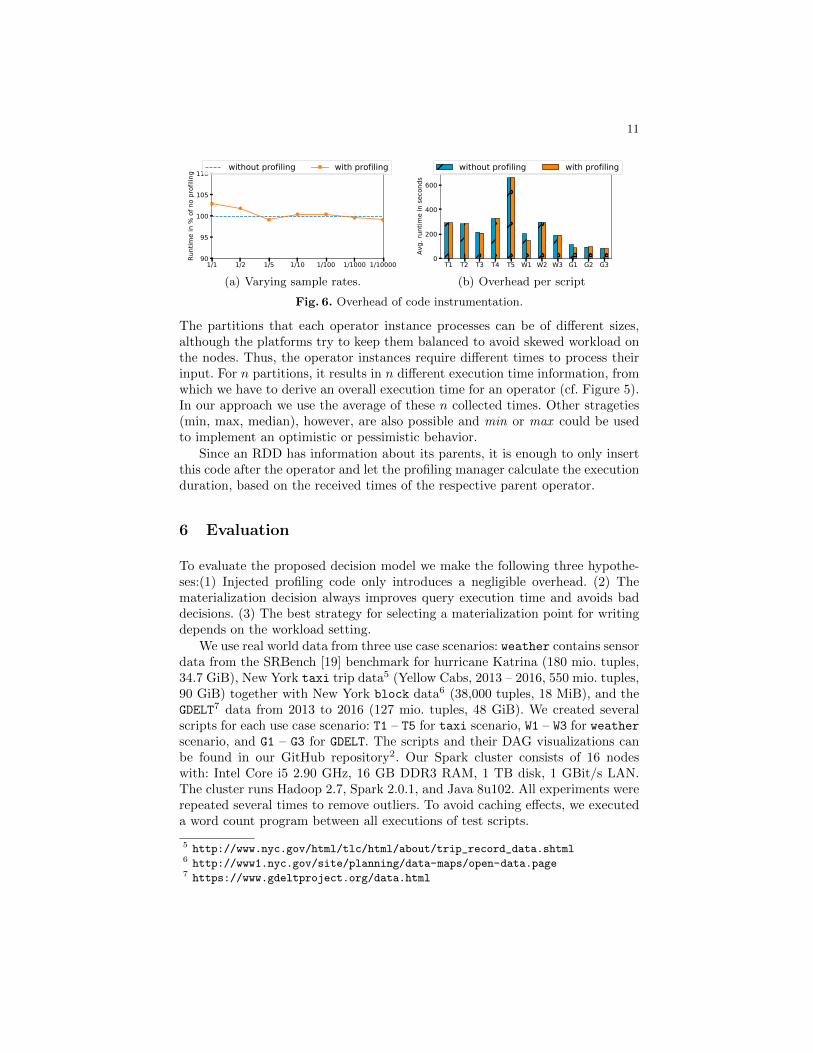
The partitions that each operator instance processes can be of different sizes,although the platforms try to keep them balanced to avoid skewed workload onthe nodes. Thus, the operator instances require different times to process theirinput. For n partitions, it results in n different execution time information, fromwhich we have to derive an overall execution time for an operator (cf. Figure 5).In our approach we use the average of these n collected times. Other strageties(min, max, median), however, are also possible and min or max could be usedto implement an optimistic or pessimistic behavior.

Since an RDD has information about its parents, it is enough to only insertthis code after the operator and let the profiling manager calculate the executionduration, based on the received times of the respective parent operator.

6 Evaluation

To evaluate the proposed decision model we make the following three hypothe-ses:(1) Injected profiling code only introduces a negligible overhead. (2) Thematerialization decision always improves query execution time and avoids baddecisions. (3) The best strategy for selecting a materialization point for writingdepends on the workload setting.

We use real world data from three use case scenarios: weather contains sensordata from the SRBench [19] benchmark for hurricane Katrina (180 mio. tuples,34.7 GiB), New York taxi trip data5 (Yellow Cabs, 2013 – 2016, 550 mio. tuples,90 GiB) together with New York block data6 (38,000 tuples, 18 MiB), and theGDELT7 data from 2013 to 2016 (127 mio. tuples, 48 GiB). We created severalscripts for each use case scenario: T1 – T5 for taxi scenario, W1 – W3 for weatherscenario, and G1 – G3 for GDELT. The scripts and their DAG visualizations canbe found in our GitHub repository2. Our Spark cluster consists of 16 nodeswith: Intel Core i5 2.90 GHz, 16 GB DDR3 RAM, 1 TB disk, 1 GBit/s LAN.The cluster runs Hadoop 2.7, Spark 2.0.1, and Java 8u102. All experiments wererepeated several times to remove outliers. To avoid caching effects, we executeda word count program between all executions of test scripts.

5 http://www.nyc.gov/html/tlc/html/about/trip_record_data.shtml6 http://www1.nyc.gov/site/planning/data-maps/open-data.page7 https://www.gdeltproject.org/data.html

12

T1 T2 T3 T4 T5 W1 W2 W3 G1 G2 G30

25

50

75

100

125

Runt

ime

in %

of '

first

run'

first run materialize recycle

Fig. 7. Three executions times for each script showing the benefit of loading material-ized results. Runtime in percent of the first execution.

Figure 6 shows the execution time without profiling as well as with codeinstrumentation for profiling for each of our test scripts. It can be seen thatprofiling incurs only a small overhead for a sample rate of 1/1 and 1/2 (meaning100% or 50% respectively are selected) and runtimes only differ in less than 10seconds or 5%. For our other experiments we selected a sample rate of 10%.

Figure 7 shows runtimes for each script for three executions. Prior to the firstexecution no statistics were available and thus are collected during this execution(blue bars). In the second execution, previously generated statistics were usedto decide which operator to materialize (orange bars). Hence, this executionincludes also the writing of the intermediate result. For the last execution thematerialized results were loaded (green bars) and thereby reduced the overallexecution time of the job.

As we argued in previous sections, scripts are often developed incrementally.In this experiment we show the runtime differences for one script of each scenariofor incremental execution (Figure 8). We first ran the according script withoutmaterialization support (dashed orange lines) and compared the runtimes to anexecution with materialization enabled (dotted blue lines). On the x-axis, step 0is the initial execution with a LOAD and a first FILTER operator and subsequentsteps add one or more operators. For the first few steps, both execution timesare equal except for some minimal discrepancies. At some point however, theoptimizer recognizes a materialization point for which a benefit will be achievedand writes the respective result to disk (indicated by vertical lines). In this step,the execution time for with materialization rises above the reference time withoutmaterialization. However, since this is executed only once, the additional costs(clearly visible in Figure 8(c)) will easily be amortized in subsequent executionsthat benefit from loading the materialized data. In fact, materialization reducedthe cumulative execution time for G1 from 7 to 5 minutes, for W2 from 30 to 20minutes, and for T5 from 80 to 30 minutes. The estimation of the benefit is animportant aspect of our approach. In our experiments we saw that the estimatedbenefits often were close to real measured speedups, but sometimes also deviatedto some extent. We observed that in almost all cases when a benefit could beachieved, we underestimated it – meaning that a subsequent execution was evenshorter than calculated. In our tests we never encountered the situation that

13

1 2 3 4 5 6 7Steps

0

20

40

60

80

100

120

Runti

me in s

ec.

with materialization

without materialization

(a) Script G1

2 4 6 8 10 12Steps

0

50

100

150

200

250

300

Runti

me in s

ec.

(b) Script W2

2 4 6 8 10Steps

0200400600800

1000120014001600

Runti

me in s

ec.

(c) Script T5

Fig. 8. Incremental execution of one script for each scenario (different y scales).

the optimizer calculated a benefit for a candidate materialization point whichactually did not bring any benefit during execution. From this we conclude thatour cost model calculates executions costs well enough to select an appropri-ate materialization point and avoid candidate materialization points that wouldcause longer execution times. Deviations are caused by our current implementa-tion of the time measurement which depends on the information of a partition’sparent(s). If the parent partitions could not be determined precisely the compu-tation of the respective operators execution time may assume a shorter or longertime.

To test the impact of the selected strategy (cf. Section 4.4) on the perfor-mance, we looked at two cases: In the first case we used additional scripts thatall share the first six operators and then diverge into their individual paths thatall contain another five operations. Strategy last did not materialize data as thelast candidate materialization point of a job will not be repeated and thus no jobbenefited from recycling and execution for each script took around 420 seconds(7 minutes). For strategies maxbenefit and markov intermediate results wererecycled and execution time was around 160 secs (2:40 minutes) for both whenresults were loaded. In the second case we disassembled the jobs from our threeuse case scenarios into a total of 132 small jobs, executed them one after theother in a random sort order and captured the time it took to complete all jobs.For strategy last the execution time was 3:47 hours, while for maxbenefit andmarkov the total time was 2:52 hours and 2:48 hours, respectively. This showsthat a selection strategy that takes the costs of operators into account achievesgood results. In this setting maxbenefit and markov created similar results, butmarkov strategy performed slightly better in this last experiment as it sometimeschose other materialization point than maxbenefit, which more subsequent jobscould recycle.

7 Summary & Outlook

In this paper we presented an approach for a cost-based decision model to speedup execution of dataflow programs by merging jobs and reusing intermediateresults accross multiple executions of the same or different jobs. The model wasimplemented in our Pig-to-Spark compiler Piglet which injects profiling codeinto the submitted jobs and rewrites them to materialize intermediate results orreuse existing results. In our evaluation we showed that profiling does not add

14

any significant overhead to execution time, that jobs greatly benefit from reusingexisting results, and that different strategies for choosing which intermediateresult to materialize are needed.

In future work we will address the problem of cache replacement as there isno infinite space for storing the materialized results and existing data may needto be removed. Furthermore, our current implementation is based on the lineageinformation of operators and could be improved by implementing strategies forquery containment checks. To address the fact that often machines are rentedfor data processing, the monetary costs of CPU cycles and storage may also beintegrated into our cost model.

References

1. S. Abiteboul and O. M. Duschka. Complexity of answering queries using materi-alized views. In PODS, pages 254–263, 1998.

2. Camacho-Rodrıguez et al. PigReuse: A Reuse-based Optimizer for Pig Latin.Technical report, Inria Saclay, 2016.

3. H. Chao-Qiang et al. RDDShare: Reusing Results of Spark RDD. DSC, pages370–375, 2016.

4. R. Chirkova, A. Y. Halevy, and D. Suciu. A Formal Perspective on the ViewSelection Problem. In VLDB, pages 59–68, 2001.

5. I. Elghandour and A. Aboulnaga. Restore: reusing results of mapreduce jobs. InVLDB, volume 5, pages 586–597, 2012.

6. A. Y. Halevy. Answering queries using views: A survey. VLDB Journal, 2001.7. V. Harinarayan, A. Rajaraman, and J. D. Ullman. Implementing Data Cubes

Efficiently. SIGMOD Rec., 25(2):205–216, 1996.8. S. Idreos et al. Merging What’s Cracked, Cracking What’s Merged: Adaptive

Indexing in Main-Memory Column-Stores. PVLDB, 4(9):585–597, 2011.9. P.-A. Larson and H. Z. Yang. Computing queries from derived relations: Theoretical

foundation. University of Waterloo. Department of Computer Science, 1987.10. T. Nykiel et al. MRShare: sharing across multiple queries in MapReduce. PVLDB,

3(1-2):494–505, 2010.11. L. L. Perez and C. M. Jermaine. History-aware query optimization with material-

ized intermediate views. In ICDE, pages 520–531. IEEE, mar 2014.12. K. Sattler, I. Geist, and E. Schallehn. QUIET: Continuous Query-driven Index

Tuning. In VLDB, pages 1129–1132, 2003.13. K. Schnaitter, S. Abiteboul, T. Milo, and N. Polyzotis. COLT: Continuous On-line

Tuning. In SIGMOD, pages 793–795, 2006.14. E. R. Sparks et al. KeystoneML: Optimizing Pipelines for Large-Scale Advanced

Analytics. In ICDE, pages 535–546, 2017.15. D. Srivastava, S. Dar, H. V. Jagadish, and A. Y. Levy. Answering queries with

aggregation using views. In VLDB, volume 96, pages 318–329, 1996.16. G. Valentin et al. DB2 Advisor: An Optimizer Smart Enough to Recommend Its

Own Indexes. In ICDE, pages 101–110, 2000.17. G. Wang and C.-Y. Chan. Multi-Query Optimization in MapReduce Framework.

PVLDB, pages 145–156, 2013.18. H. Z. Yang and P.-A. Larson. Query Transformation for PSJ-Queries. In PVLDB,

volume 87, pages 245–254, 1987.19. Y. Zhang et al. SRBench: A Streaming RDF / SPARQL Benchmark. In ISWC,

pages 641–657, 2012.