Cost Allocation Methods for Workers Compensation
40
Cost Allocation Methods for Workers Compensation George M. Levine, F.C.A.S. 163
Transcript of Cost Allocation Methods for Workers Compensation

Cost Allocation Methods for Workers Compensation George M. Levine, F.C.A.S.
163

Cost Allocation Methods for Workers Compensation
George M. Levine
With the recent growth of alternative risk financing for workers compensation, in retrospectively rated insurance programs, high deductible insurance programs, self- insurance trusts, captives, and other insurance programs, cost allocation methorls for workers compensation funding is an increasingly important, If not overlooked, subj’ect matter. This paper presents a cost allocation methodology for workers compensation, and will develop dtflerent approaches for allocation.
Due to the heightened awareness of workers compensation and safety during the past decade, many cost containment programs, legislation changes. and medical cost containmentprograms have been initiated Workers compensation chargebackprograms can be one important 1001 in the containment of workers compensation costs. Given this development. the allocation of those costs have become crucial management issues for business. The interaction o/OSHA statistics and workers compensation losses will be discussed, as both sets of statistics are important in the management of workers compensation costs.
The benefit of this paper is to document diflerent techniques for cost allocation, to show the pros and cons of the various methods, and to explore the ramifications for COSI allocation upon loss control techniques.
Biography
George Levine is a senior consultant in the Hartford, Connecticut office of KPMG Peat Marwick, LLP. He holds a Bachelors of Science Degree in Economics from the Wharton School of the University of Pennsylvania, and a Masters in Business Administration from the University of Connecticut. George is a Fellow of the Casualty Actuarial Society and a member of the American Academy of Actuaries. He is a past member of the American Academy of Actuaries Committee on Property and Liability Issues, and currently serves on the Casualty Actuarial Society’s Editorial Committee for the Proceedings. George has authored a discussion of a paper in the Casualty Actuarial Society Proceedings titled “An Analysis of Excess Loss Development” and participated in the 1985 Discussion Paper Program.
The author would like to thank Roger Wade, Robert Miccolis, Patricia Teufel, Norman Bailis, and Jack Braddock for their support in preparing this paper.
164

COSI AllocaIion for Workers Compensadon
I. Introduction
During the early 1990s the cost of workers compensation became an important
competitive issue to United States industry. Together with health insurance, the costs of
workers compensation became a competitive millstone for many U.S. businesses. For
example, it comprises upward of 20 percent of the total wage bill of Detroit auto makers,
as opposed to 8 percent for their Japanese counterparts. The role of the actuary in
assisting in the control of workers compensation costs became increasingly important,
whether it was to price benefit changes, assist in the design of retrospective rating plans,
price assigned risk plan charges, or in the allocation of costs. The downward trend of
workers compensation costs during the last four years was aided by effective cost
allocation plans. It is increasingly important for the actuary to understand cost allocation
systems if the actuary is to remain a “player” in the arena of workers compensation,
In this paper. the methodology of one such plan will be outlined, which allocates costs for
the prospective funding period to organizational units. The costs for the reserves (prior
funding periods) will be discussed below, but these costs are not the focus of this paper.
The technique will be critiqued, considering seven goals of an allocation system. Next,
important features of a loss control plan will be presented, and the manner in which a cost
allocation plan supports those desirable features will be supported. The rationale for
165

Cost Allocalion for Workers Compensation
OSHA safety statistics, and how those statistics relate to workers compensation statistics
will be presented. Finally, an allocation system to the “micro” level will be presented.
2. Purposes of an Allocation System
. . The Casualty Actuarial Society’s Statement
p provides four principles and eighteen considerations
relating to ratemaking. For a cost allocation system for funding, many of these principles
and considerations are important in any actuarial ratemaking methodology. According to
Fritz[Z], there are six uses of a cost allocation system which are listed below,
accompanied by the relevant ratemaking consideration or principle from the Statement of
Principles.
Uses of an Allocation
I. To distribute costs fairly
2. To ensure each unit pays its own way
3. To subsidize smaller units
4. To focus attention on loss control
5. To stabilize budgeting for units
6. To provide a management tool
No unfair discrimination
Homogeneity
Individual Risk Rating
None
Credibility
None
166

P
Cost Allocation for Workers Compensation
The absence of a ratemaking consideration or principle which matches with the use of an
allocation system illustrates the historical lack of involvement for actuaries in the
management of workers compensation. The statement of principles does suggest that the
actuary has a key role in the interaction with other disciplines such as underwriting,
marketing, law, claims, and finance. Management and loss control can be added to that
list, as cost allocation can be a significant motivator to the management of workers
compensation costs. For management, the setting and realization of annual cost goals can
provide incentives to control costs. Sending messages regarding rewards and penalties
can also be an important tool in workers compensation. It is the informed actuarial
judgment, the eighteenth consideration in a ratemaking system, that is important in a cost
allocation methodology.
Another consideration in selecting a cost allocation methodology is the match between
the corporate structure and the projection methodology chosen. For example, a
decentralized corporate structure, with each individual unit a profit center designed to
stand on its own, might suggest a cost allocation scheme designed for more loss
sensitivity. On the other hand, a centralized corporate structure might call for more
smoothing of individual business units’ loss experience, as there would not be a great
need for differing funding by unit.
167

Cost Allocation for Workers Compensation
3. Projection Group Technique
The following system can be used to allocate costs on a “macro” level, i.e. to the larger
organization units. First, the technique will be presented, and the manner in which the
ratemaking considerations impact the technique will be discussed. Next, how closely the
technique achieves the desirable features will be presented, along with the conflicts
inherent in any allocation system.
Methodology Description
Exhibit I presents a projection group technique, which combines’four business units into
one projection group for funding purposes. This paper defines projection group as a
group of data collected together solely for the purpose of developing a funding level.
Certain actuarial characteristics such as homogeneity, suggested by the ratemaking
principles discussed above, help determine the composition of such a group, made up of
several business units. In addition, a business unit is defined as a unit in an organization
which exists, such as a profit center or a major division.
The methodology can be described as a ratemaking methodology based on a five year
weighted average by business unit, but with overall rates controlled by the combination
into one projection group.
168

COSI Allocarion for Workers Comwnsation
Each individual business unit’s rates and funding are presented on Exhibit I. Sheets I
through 4. The following describes the procedure for the allocation method.
Step 1. Develop individual business unit data funding, no trend
The following is a brief description of the mechanics of determining the funding level for
business unit one, Low Exposure Groups. Here, business units judged to perform low
exposure labor, such as light manufacturing. are combined. The other business units
funding levels are determined in a similar manner. In this example, funding is
determined for all of the business units at a $500.000 retention level. Although retentions
of $100.000. $50.000. $50.000 and $250.000 are used for business units I through 4,
these are actuarial internal mechanisms to introduce stability for the units. Ultimately, all
of the units are funded IO a $500,000 level.
Business Unit I. Exhibit I. Sheer I
(For the purposes of this paper. the term division and business unit are used
interchangeably).
I. Exposure Unit
169
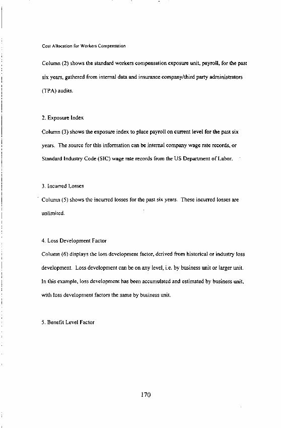
Cost Allocation for Workers Compensation
Column (2) shows the standard workers compensation exposure unit, payroll, for the past
six years, gathered from internal data and insurance company/third party administrators
(TPA) audits.
2. Exposure Index
Column (3) shows the exposure index to place payroll on current level for the past six
years. The source for this information can be internal company wage rate records, or
Standard Industry Code (SIC) wage rate records from the US Department of Labor.
3. Incurred Losses
Column (5) shows the incurred losses for the past six years. These incurred losses are
unlimited.
4. Loss Development Factor
Column (6) displays the loss development factor, derived from historical or industry loss
development. Loss development can be on any level, i.e. by business unit or larger unit.
In this example, loss development has been accumulated and estimated by business unit,
with loss development factors the same by business unit.
5. Benefit Level Factor
170

Cost Allocation for Workers Compensation
Column (7) displays the benefit level, derived from NCCI benefit level history by state
within business unit. Because the state composition differs by business unit, the benefit
level factors in this example differ by business unit.
6. Trend Factor
The trend factor, Column (8), can be derived from industry or projection group
experience. The trend is derived after the business units have been combined into a
projection group. For now, the trend is set equal to 1 .OOO.
7. Adjusted Losses
Developed, on-benefit level, and trended losses (for now, trend equal to I .OOO) are
displayed in Column (9).
8. Losses in Excess of Division Retention
Individual losses which are developed, on-level, and trended in excess of the retention are
shown in Column (IO). Individual loss runs are necessary for this column. The limited
losses are shown in Column (I l), as column (9) minus column (I 0). Note that the
division retention is $lOO,OOO.
Some actuaries may propose an alternative of limiting losses to retentions as a first step,
with loss development and trend as subsequent steps. This would be appropriate, as long
as any losses exceeding the retentions after application of excess development and trend
171

Cost Allocation for Workers Compensation
are deducted.
9. Limited Loss Rate
Column (11) divided by column (4) produce the limited loss rate, displayed in Column
(12).
Step 2. Select Loss Trend Factor, for Projection Group
tier similar data compilations for business groups 2 through 4, developed and on-benefit
level losses and rates are developed and summed on the projection group page, Exhibit 2,
Sheet 1 I Column (12). A review of the loss rates show a 3% increasing trend; this trend
can also be selected based on industry statistics. For workers compensation, a separation
of this exhibit into indemnity and medical components might be an improvement. Once
the trend is selected, the trend rates are selected for all other groups as well. For this
exercise, it was determined that a common trend rate was appropriate for all the business
units. Another possibility could be to select different trends for the divisions, and then
summing in the overall projection group.
Step 3. Select Projection Group Loss Rate
On line (13), a selected projection group loss rate for all divisions has been selected as
$32.00. It is through the projection group selected loss rate that the actuary exercises the
172

Cost Allocation for Workers Compensation
control over the funding level; the remaining steps are to allocate the loss funding level
back to business unit. Once the individual units’ losses are determined based on the five
year weighted average basis and credibility weighted (discussed below), these losses are
summed on line (I 6). The “balance” factor, or off-balance factor as used in some
actuarial literature, is the selected projection group losses divided by the sum of the
division losses, line (I 7). This balance factor is then applied to the individual business
unit losses on line (20) of each business unit’s sheet (discussed below) to sum to the
desired funding level.
Step 4. Determine Loss Funding by Business Unit
The individual business units’ trended losses and rates are shown on Exhibit 3. The
following are the calculations to determine final funding by business unit, with the review
of the exhibits’ figures beginning from Line (13).
173

Cost Allocation for Workers Compensation
/ I. 5 Year Weighted Average Limited Loss Rate
The sum of Column (I I) divided by column (4) for the past five years produces the 5
year weighted average limited loss rate, displayed in Line (I 3). Five years is used to
introduce stability.
2. Increased Limits Factor to $500,000
The increased limits factor on line (14) is derived from NCCI Excess Loss Factors, or
determined based on internal company studies. This brings the loss rate from a $100,000
to %SOO,OOO level on line (I S), through multiplying the limited loss rate on line (13).
3. Projected Group Loss Rate Limited to $500,000
Line (16) displays the selected Projected Group Loss Rate from Exhibit 3, Sheet I. This
is the expected loss rate to which the complement of the credibility weight, determined on
line (I 7), will be applied.
4. Credibility Weight
Line (I 7) displays the credibility weight for the division, determined by the formula of
[line (24)/$100,000]“.5, with line (24) representing projected payroll.
174

Cost Allocation for Workers Compensation
5. Credibility Weighted Loss Rate
Line (I 8) displays the credibility weighted loss rate for the division, determined by
weighting the division loss rate by the credibility weight, and the complement of the
credibility by the projection group loss rate.
6. Losses Before Balance Factor
The business unit’s losses before the balance factor are displayed on Line (19). as the
product of line (18) and the projected payroll, line (24).
7. Final Loss Rate
The business unit’s final loss rate is determined on line (2 I) as the product of line (I 9)
and the balance factor, line (20), as produced on the projection group’s summary sheet,
line(l6).
8. Final Funding Determination
Lines (22) through (29) determine the funding levels after the actuarially determined loss
rates of line (21). Note that the variable expense loading, for self-insurance fees, second-
i/
Cost Allocation for Workers Compensation
injury fund charges, state taxes, assigned risk charges, boards and bureaus charges, and
loss conversion fees. normally associated with retrospective rating platis, are shown on
line (22). Fixed expenses and excess premiums, associated with claims handling fees,
brokers fees, actuarial fees, and purchase insurance in excess of the $500,000 retention,
are displayed on line (27).
Critique of the Methodology
C According to Fritz, six desirable features of any allocation system are simplicity, fairness,
flexibility, accurate and readily available data, mechanization, and loss sensitivity.
Another issue is to what extent the ratemaking considerations from the Statement of
Principles Regarding Property and Casualty Ratemaking are accommodated. The
following assesses how the projection group methodology fares with those goals.
Simpiiciy
This methodology, although simple enough to apply with modem spreadsheet
technology, is daunting to the non-actuarial world. To follow the numerous steps
describe above is relatively time-consuming for the layperson. Most actuaries would find
the methodology rather straightforward, especially when the assumptions are well
documented.
176

Cost Allocation for Workers Compensation
I Fairness
The methodology utilizes the own business unit’s own experience to the extent possible
through credibility considerations. Some might complain that other units’ experience, if
worse than that business unit’s experience, unfairly influences the funding level. In that
case, higher credibility could be allocated to a business unit’s allocation; at the extreme,
100% credibility could be assigned and one could move away from the projection group
methodology towards a division standing on its own. Changing the division’s retention
level could also be a method to introduce more sensitivity if desired, to get away from the
use of the industry increased limits factors.
A commonly overlooked issue of fairness. which is discussed below in the “micro”
allocation level. is the use of relatively “old” data. In the rapidly changing organizational
structures of the modem organization, the retention of data five years mature for the
assessment of divisional charges could be perceived as unfair. It is the use of this mature
data in rapidly changing organizations, which although may be actuarially “sound”, is
fundamentally flawed, especially when used for performance measurement. Even data
hvo years old can be viewed as stale. The lack of “real-time” data, combined with a
changing organization, could be perceived as a significant flaw of this approach.
177

Cost Allocation for Workers Compensation
Flexibility
This approach is extremely flexible, with mechanization tools. Retention levels can be
changed, credibility formulas may be adjusted, and groupings of business units’ data
within projection groups can be rearranged to reestimate funding levels. The use of a
projection group allows the necessary actuarial control to be provided over the funding
level.
Accurate and Readily Available Data
The use of many data base management systems allows for readily available data on a
quarterly basis. The accuracy of the data is mostly in the control of the insurance
company, insured, and third party administrator.
Mechanization
The system is mechanized easily through spreadsheets, and is determined after one or
two iterations for trend. One might wish to save prior versions before trend selections are
made for later review.
178

Cost Allocation for Workers Compensation
Loss Sensitivity
The approach under certain circumstances can be made to produce funding levels not
sensitive to actual loss experience, as the loss limitations, credibility, and projection
group approach can make any changes to the funding level based on loss differences
practically imperceptible. For example, a low loss limitation, low credibility, and
inclusion in a larger projection group can reduce sensitivity to loss experience. This
insensitivity can be adjusted through the micro allocation methods described below.
Actuarial Ratemaking Considerations
From an actuarial perspective, the methodology accommodates many of the actuarial
considerations from the Statement of Principles. The determination of the exposure unit,
the data organization, homogeneity and credibility considerations, loss development and
trends, catastrophe considerations, individual risk rating, investment and other income,
and actuarial judgment are ten considerations well accounted for in this methodology.
Additional considerations to risk, and operational changes by business unit are
opportunities for improvement for the methodology.
179

Cost Allocshm for Workers Compensation
4. Workers Compensation Chargeback System
Although a cost allocation system for workers compensation can be actuarially sound,
f!rom a loss control perspective it can be rather ineffective. The use of mature data can be
considered a good predictor of future costs, but irrelevant to the rapidly changing modem
organization. For that reason, a more real-time allocation system can be employed, to
implement a system more weighted to current data. Many of the data base management
systems developed by the insurance industry can be used to extract the data. The cost
allocation system proposed here would be to take the cost allocation on a business unit
level, and develop a system to allocate those costs on a “micro”, or more detailed level.
Exhibits I through 3 from above define annual funding for a major business unit. Below,
funding on a more timely basis, by month, to a lower level is described, which is defined
here as a chargeback system. Both the projection group approach and the chargeback
system are prospective methods, although the base periods will be different as shown
below. The following describes the chargeback system approach; first, a brief description
of OSHA statistics is provided to demonstrate how this approach relates to the QSHA
statistics.
180
Cost Allocation for Workers Compensation
OSHA Incidence and Severity Rates
The US Bureau of Labor Statistics publishes statistics on occupational injuries and
illnesses. Two common OSHA statistics are incidence rates and severity rates. An
incidence rate is defined as the number of injuries and illnesses per 100 full-time workers,
and is calculated as:
(NIGH) x 200,000, where
N= Number of injuries and illnesses
EH= Total hours worked by all employees during the calendar year
200,000= Base for 100 equivalent full-time workers
(working 40 hours per week, 50 weeks per year)
A severity rate is defined as the number of days away From work per 100 full-time
workers, similarly as follows:
(YEH) x 200,000, where
s= Number of days away from work
EH= Total hours worked by all employees during the calendar year
200,000= Base for 100 equivalent full-time workers
(working 40 hours per week, 50 weeks per year)
181

Cost Allocation for Workers Compensation
These two statistics seem to correspond to the frequency and severity statistics of
insurance companies. The two important differences are that the severity statistic for
OSI-IA lacks financial figures, and often indicates different trends from insurance industry
information. Additionally, these statistics are published annually by the Bureau of Labor
Statistics, but most companies publish them internally monthly to be made available for
senior management review. It should be noted there are often differences between
insurance industry and OSHA claim definitions. However, these statistics are publicly
available and are important benchmarking statistics for many organizations. The IBNR
nature of claims is also not available for these statistics; these injuries are simply recorded
as they are repotted. A detailed explanation of the OSHA statistics is provided in the
Appendix.
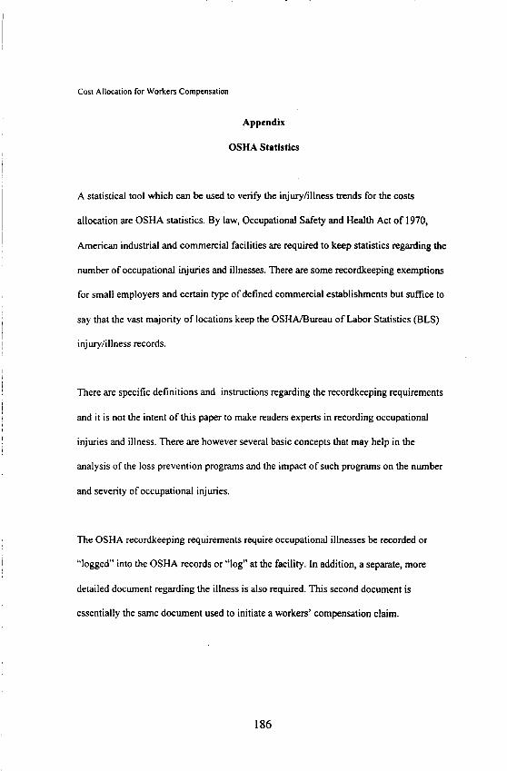
Workers Compensation Chargeback System
Due to the rapidly available OSHA statistics, it is important to develop a system to
allocate costs to a more microcosmic level on a timely basis. Here, the annual funding is
“charged back” to very tine business units, which are called “site codes”, on a monthly
basis. One could simply allocate a fixed cost (l/l2 of the annual cost) each month, but
incentives to understand or manage losses might be lost. For this example, the objective
is to allocate the annual 6527,140 business unit 4 charge to the hvo “site codes” which
comprise the business unit, for a monthly charge. In many organizations, responsibility
182

Cost Allocation for Workers Compensation
levels are much smaller than the business unit levels described here for financial
purposes.
The methodology illustrated on Exhibit 4 is to compute a rolling calendar year average
of workers compensation losses and lost-time injury counts to allocate the costs to a
lower level. Its advantages are the responsiveness of the charges to actual experience, its
simplicity, and the flexibility within the organization. New site codes could easily be
accommodated. In this example, a six-month rolling average is utilized. This system is
significantly skewed towards a reward/penalty type experience rating approach; it is
conceivable that a smaller unit could be allocated all costs, if no other unit incurred losses
over a time period. It fits well with the overall actuarial goal, where the costs have been
determined on a basis accommodating actuarial principles. With a modem risk
management data base system, this method can be easily adapted. The methodology does
not meet many of the actuarial considerations from the ratemaking principles, such as
homogeneity and credibility, and could be judged as unfair and too sensitive to large
losses.
It should be noted that the author was part of a cross-functional team of cost accountants,
plant managers, risk managers, and health and safety professionals which designed this
chargeback system. The team debated whether OSHA statistics should be included as
part of the chargeback system; however, the final conclusion was that OSHA statistics
were only an indirect measure of workers compensation costs.
183
Cost Allocation for Workers Compensation
5. Conclusion
This paper has demonstrated a sound actuarial methodology to allocate costs within an
organization on both macro and micro levels. The approach has the advantage to be
actuarially sound, while accommodating loss control and other organizational goals. This
area can be researched further in the future, to provide other areas where actuaries can
apply expertise in growing areas.
Additional research into areas such as allocation of expenses, large loss capacity by
division and in total, and credibility are suggested by the projection group methodology.
184
Cost Allocation for Workers Compensation
Bibliography
[I] Angelina, Michael E. “Allocating Risk Financing Costs”, Casualty Loss Reserve
Seminar, September 19, 1995.
[2] Fritz, Carol. “Allocating Risk Financing Costs”, Casualty Loss Reserve Seminar,
September 19, 1995.
[3] Senge, Peter M. 3
-Currency Doubleday, 1990, New York, p. 326.
185
COSI Allocation for Workers Compensation
Appendix
OSHA Statistics
A statistical tool which can be used to verify the injury/illness trends for the costs
allocation are OSHA statistics. By law, Occupational Safety and Health Act of 1970,
American industrial and commercial facilities are required to keep statistics regarding the
number of occupational injuries and illnesses. There are some recordkeeping exemptions
for small employers and certain type of defined commercial establishments but suffice to
say that the vast majority of locations keep the OSHMBureau of Labor Statistics (BLS)
injury/illness records.
There are specific definitions and instructions regarding the recordkeeping requirements
and it is not the intent of this paper to make readers experts in recording occupational
injuries and illness. There are however several basic concepts that may help in the
analysis of the loss prevention programs and the impact of such programs on the number
and severity of occupational injuries.
The OSHA recordkeeping requirements require occupational illnesses be recorded or
“logged’ into the OSHA records or “log” at the facility. In addition, a separate, more
detailed document regarding the illness is also required. This second document is
essentially the same document used to initiate a workers’ compensation claim.
186

COSI Allocation for Workers Compensation
Occupational injuries are handled differently in that the relative severity of the injury has
to be considered before the injury is recorded. To be a recordable injury, the injury has to
require more than ftrst aid treatment. Any injuries resulting in loss of consciousness, job
change or job restrictions or days away fium work are recorded. OSHA does not address
who provides the treatment but rather the type of treatment provided. In workers’
compensation data bases the fact that treatment is provided by an in plant EMT rather
than a hospital emergency room is important as one generates a cost and subsequent file
andone does not. The same issue does not apply in the OSHA recordkeeping decision
model as the issue is what type of treatment is provided, not where and/or by whom. As
with the occupational illness cases, the injuries are recorded or “logged” with more
detailed information recorded on a separate form. In many jurisdictions the separate form
used to record additional data regarding the injury is the same form used to report a
workers’ compensation claim.
OSHA frequency rates are based on the number of cases recorded. Comparison with
workers’ compensation frequency data can be made. However, some caution has to be
taken as the definitions in different jurisdictions determine what type injuries or illnesses
are considered job related for workers’ compensation benefits. Examples where there are
major differences include sports injuries; they typically not recordable under OSHA
requirements but in some jurisdictions may be compensable under workers
187

Cost Allocation for Workers Compcnsarion
compensation; parking lot injuries (may not be recordable under OSHA/BLS guidelines,
may be compensable under workers’ compensation statutes), hearing loss (extent and
whether active retired employee may affect recording outcome) and even some
occupational illnesses which may not be recognized in certain jurisdictions as an
occupational disease for workers’ compensation benefits.
While fiquency comparisons may not produce a one to one relationship, they can
produce some comparative trend illnesses assuming the number of cases is large enough
to make such comparisons effective and differences based on definitions are understood
and considered in the analysis. Not every case which results in a workers’ compensation
claim will be recorded as an OSHA injury and the likewise not every OSHA recordable
case will be a workers’ compensation case. Loss prevention and loss control programs
that reduce the workers’ compensation costs should also have a positive impact on the
OSHA rates.
OSHA measures severity in terms of the number of days the employee is away from work
or the number of days the employee is restricted. While there may be some correlation
with severity measurement based on dollars, the definitions in the various jurisdictions
have to be considered in any comparisons. An example is scarring awards. One
jurisdiction had a scarring award which paid out indemnity benefits for injuries which
often were treated in in-plant clinics and may not have been OSHA recordable. If they
188

Cost Allocation for Workers Compensation
were recordable under the OSHA recordkeeping system they did not result in lost time or
restrictions and would not be considered severe but would result indemnity payments
which would make it a more severe case in the traditional workers’ compensation
statistics.
The number of cases and number of days are then used to generate rates which facilitate
comparisons, either internal and/or external. The key indices include the Total
Recordable Rate, the Days Away From Work Incidence Rate, the Lost Workday
Incidence Rate, the Days Away From Work Severity Rate and the Lost Workdays
Severity Rate; the rates are calculated as follows:
(N/EH) l 200,000 = Rate where EH equals the actual hours worked
If N is the total number of injuries and illness, the rate is the Total Recordable
Incidence Rate (TRIR)
If N is the number of cases resulting in Days Away From Work, the rate is the
Days Away From Work Incidence Rate (DAFWIR)
If N is the number of cases resulting in days away from work and/or days with
restricted work, the rate is the Lost Workday Incidence Rate (LDIR)
If N is the number of total number of days employees lose as the result of
occupational injuries and illnesses, the rate is the Days Away From Work
Severity Rate (DAFWSR)
189

I - /-
Cost Allocation for Workers Compensation
If N is the number of days employees are away born work and/or prevented from
performing all of their regular work, the rate is the Lost Workday Severity Rate
(LDW
The 200,000 is used in the calculation to normalize the rates to 100 employees. The
200,000 is based on 100 employees working 40 hours a week for 50 weeks of the year.
A representative number of employees annually submit their safety performance statistics
to BLS where rates based on SIC (Standard Industrial Classification) Codes are
published. The rates enable comparisons with other similar industries based on the SIC.
In addition the BLS data enables comparisons with facilities-of various sizes. In addition
BLS publishes information regarding quartile performance so that comparisons can be
made with other facilities/companies with the same SIC code.
In many companies the safety statistics are tracked with workers’ compensation data.
Over time comparisons can be established; however, because of difference in definitions
and interpretations in the various jurisdictions make one on one trending difftcult. Sufftce
to say that trends in reducing the frequency and severity of occupational injuries and
illnesses using the OSHA definition should also result in measurable reduction in the
workers’ compensation costs. Indeed OSHA recognizes tbis relationship and uses state
workers’ compensation data to focus their inspection activities as they believe that those
190

Cost Allocation for Workers Compenwion
employers/facilities with the highest number of workers’ compensation claims are the
same employers with deficient safety and health prograins.
Use of the OSHA injury and illness rates may provide another tool for evaluating the
effectiveness of loss prevention and loss control programs and as a means of allocating
costs provided the user understands the similarities and differences which are inherent to
comparisons involving workers’ compensation claim data and OSHA incident data.
191

Fmhg 6~ Fmd Yw 719598 11109/95 Projicbm Gmp: 1 D+&im1F~Devehpmsnt
Davisin Nuna. Business unit 1 Exposlwe Base paw w-1 SlOO.MO 11w.ml
Llxaesh Limited Lvrmad
PW G
Bmefil E- Ad)ussad LOSS b Yeaf ET-=- Adiusted lncwrad LsVd LCX-9 Adjustad Excasa of Lc5sas 6 Erpen=
B@+P+m Elpowne Index Eve Lossas F& F&U Tld L- s1co.alo Ekpensas Rsle
(1) (2) (3) (4) (5) (6) (7) (a) (9) (10) (11) (12) ._--_-_
7lao 29.547 I.223 36.136 442646 1.168 0.980 l.oa, 565.015 114.502 396.513 7189 30.055 1.196 35.645 449763 1.227 0.959 i.mJ 529.205 64.731 444.474 7m 33,215 1.137 37.834 s99m9 1.166 0.959 l.om 670.276 14.926 655.352 7191 4~.000 1 IO1 47.343 563439 1.333 0.955 IO%3 717.116 110.co3 607.113 7192 5J.000 1.068 56b.bol 631362 1.711 0965 l.OW 1.372,136 35.335 1.336.603 7l??i 63.000 1.045 65.635 679250 2 270 0697 1.6W 1.537,563 0 1.537.503
TOW 251.67? 27’9.397 X665.791 5.331.2itl 35a.499 4.971.756
w (14) (15) (16) (17) w (19) (W (21)
m (a
(24) (23 (W (27) m (W
5YssrWd&tdA~LtmhdLossR.h: Imxeamd Lbrils Fwtar to S6CO.tkXI hvtbmol Loas Rata at s54lo.am Prcj GKql Lose Rata Linhd to s!xcl.Lmo: cfEdblQw* CradildUy Weightad Loss Rate: Losses Before Bakwx Fzdci Bahnm Fatm 7195 Las Rate:
16.63 1.160 21.68
32.alo 0.606 2366
v-x~ 1.156 27.35
7185 Vatable Eqmme Factor: 7195 kaud Rata:
l.oBS 29.234
7195 Prol&(d Eqmaum: 65.006 7195 Losaea h VaIlam Erpmwa: 1.900.165 7/95l)immmdL.n6ea6vY~: 1393.976 7195 Fkmd Gcpamn 6 Ercaa Premiums: 170,151 7l96 Tdd UM Acud: 2.070.136 7195 Totd Dismu~tad AMPI: 1.1644.127
1061 12 47 17.32 12.62 23.62 23.35
17.79

EhibiIl shad2
Fmding for FuW Year 719566 Plojmm Gmup’ 1 Divkim2FundingDevebpmnt Dnch Name: BlKiMssllni(2 Eqmscne Base: Pwd mw
L-6
F-3 LOSS Bmldil W-.=3 YS4 E-0 Adjusted lrlcwred Dn”~ Levd Loss Adjuded Excess d
Bm Erposlrre l&r EW=- LOSsaS Fklor FXbX Trend L- S50.000 (1) (2) (3) (4) (5) (6) (7) w (9) (10)
_.... - --.. - --._ ~ ---_ -- --..-- _.-- - -- ---
llm9B5
SWYX SSo.MO Limb6 Limited
Mjuskd Loss 6 L-6 Expenss ET=== Rata
(11) (12) ---
716a 4.464 1.223 5.459 375040 I 077 1.1m loo0 476.93 32.592 443.951 61 32 7189 1.351 1.186 6,355 291566 1.122 1.115 1.060 364.826. 50.100 314.725 49.53 7m 4.511 1.137 5.131 512129 1.191 1036 loo0 669.%3 113.524 555.439 108 44 7191 5.oml 1.101 5.505 3ooM7 i.mr 1.087 1.ooo 425.476 6.576 41e.e9.9 76 09 7192 1.018 10% 6.585 318074 1.492 10% 1.0% 505.413 21.504 483.909 56.37 7193 6.171 1.045 7.078 137217 1.601 1.047 r.ow 253.792 0 258.792 36.56
TOtd 34.146 38.113 1.934.834 2.701.012 224.299 2.478.714 6496
(13) (14) ((5) @I (17) (16) WI (m PO
cm cm
(24) (m cm (271 cm (2%
5 Yea Wal@td Aw LMtd Lou Rats lnuaaed Llmils Facbx to SXQXIO: Dkkmd Loss Rdn d S%IO.~~: Prd Graq Lms Rate LbAted lo $%X1.000: crddi6ly wal@t CfadWy We&htad Less Rate;
Losea fJ&re Baknca F&or BdFotoc: 7195 Laa Ram
62.25 l.za, 74.70
32.m 0265 43.30
303.D66 1.158
50.042
7rBJ Vmtdh Eqmsa Facbx. 7195 Acuud Rata:
1 .oso 53.494
7195 Projacw E%posuras: 7.000 7195 L- 6 VtiLh Expanses: 374.461 71?t5 -M Losses 6 Vat E-w: 274.705 7JS6 Fbrsd Expmsm h Evasa ~rsmiums: 143.122 7IS5 Togl thxkuxmled ACUU& 517.563 T&5 Tdd Dkcwnlad bxzud: 417.627

Etibil 1 Sheet 3
Funding lor Fund Year 7195.96
1 Division 3 Fwulii Development
Business Unit 3 Payroll (CmS) s50,om
hwes 6 Llllad LOSS Benem EXpOtlSM Adjusted
Exposure Adjusted Incurted Developnent LOWI LOSS Adjusted EIcesod Losses 5 Index EIpOSUW3 LOSS.%% Factor FilCtOf Trend L- S5O.ooO EXp.%lS.%
(3) (41 (5) (6) (7) w (9) (10) (11) ---_......_ -.- -___-.._- --__.-- - __.._._.-- _- ----_ .__ ___I ----- ---~-
Pmjectm Group: Dwision Name E:posure Base
Policy Y.Vll
Eegmng E1posllra
(0 (2) . . . . ..-- - .-_. ---.._.--
7188 12.993 1.223 15.a54 160075 1.077 1.042 I.000 202.066 0 202.066 7189 15.935 Il.96 18.902 25569 1 1.122 1064 1.0&l 310.984 31.191 279.793 7193 20.677 1.137 23.510 150669 I 191 1.067 l.lXW 191.470 56.442 135.020 7191 14.235 I 101 15.674 92276 I 301 1.054 1.006 128.534 0 126.534 7122 15.571 1.066 19.834 132779 1.492 1045 l.ooO 207.021 15.920 191.101 7193 14,611 1.045 15.268 160532 1.801 I 036 1.000 336.843 37.069 239.774
S5O.ooO Limited Loss L
EXpelW Rate
(12) I-.
12.75 14.60
5 74 807 964
19.63
TOM 86.996 109.042 992.022 1.374.Fr39 140.622 1.X44.315 11 32
(13) (14) (15) (16) (17) (18) (19) m (21)
w3 (23)
(24) (a WI 07) (28) m
5 Year Welphtd AVQ Limited Loss Rate. Incmased Lii Fecta to $500.000: Dwisii Lam Rate at SS00.000: Proj Group Loss Rate Lii to S%YJ.oM credibility waight: crw weighted Loss Rate: Losses Before Balam Fa~tm Eabnu, Fa~tw: 7195 Loss Rats:
1106 1.2M 13.29
32ooO 0.4% 236.9
450.035 1.156
27.595
7195 Vuipbb Eqmso Factor: 1.069 7195 Accnml Rata: 29.501
7195 Projected Erporurm: 15,950 7195 L- 6 vatiabta Eqmmm 558.085 7196 D-ted LOCBBS 6 VW Erpenses: 407.944 7195 Fii Expemus 6 Enxss Premiums 66,052 7195 Totat Undisamted kcmat. 622.137 7/95 Total Diinted AMlal: 471,996
lllW95

; E-1 sheet 4
Funding la Fwrd Year 7/9596 Projecthan Group: 1 Dii 4 Funding Developmmt Diikion Name: Business unit 4 Exposure Base: Payrdl (CmS)
P&y LOSS hefit Year EXpoSlUS Adjusted lncurmd DwelopMnt Level LOSS AdjlLstad
Eeginning Erpxwe hlex EXpOSUfS LOSSSS FSCtW FaCti TMld L0S.W
(1) (2) (3) (4) (5) (6) (7) @I (9) -.-----.-- -. -.----- _---___ - _____ --- ---- L_- _--I_
llm95
S25O.OtKl S250.m0 L-6 Llniled LhitSd Expenses Adjusted LOSS6 Excess of LoemSh Em-
5250.ooo Exp.rusr RStS
(10) (11) (12)
7189 6,245 .I.223 1.638 389479 1.077 I. 228 1.&w 514,269 99.907 414.362 5425 7189 7,907 1186 9.449 506020 1.122 I. 137 l.ooO 645.537 0 645.537 68 32 7Ea 9,927 I. 137 10.038 757448 1.191 1.117 l.ooO 1.007.669 162.383 625,306 82.23 7191 9,997 1.101 7.583 538425 1xX I. 105 l.coo 774.042 87.037 666.205 9050 7192 9,564 I.068 10.15e 433598 1.492 1.079 1.000 698.039 47.828 650.210 64.W 7f93 7.306 1045 7,635 510875 1.801 1.058 IXWO 973.451 418.910 556,541 72.90
TOM 46.738 52.490 3.135645 4,613.LXU 034.042 3.776.161 71.98
(13) (14) (15) (16) (17) (I@ (1% w-3 (21)
m (2%
(24) (=I @a (27) Gw m
5 Ysar W&hW Avp Limiiad Loss Rate: Increased Lhth Factor to S5CCt.ooO: DM6ic.d Loss Rata al S5OJ.Mo: Proj Group Lou Rate Linhd to S5oo.oM: cmdititity wdght CWibiBty W&hted Lms Rate: L- B&m 83ance Factm Balams Factm 7195 Lass Rate:
7195Vti I5qm.a Factor. 7l95 - Rala:
7835 Projsbd ExpLmufm: 7195 LOSSSS A VariaWe Expmm: 7l96DtscantedLo~a~~hVuEx~~n~~~: 7% Fkd Expases 6 ExcnS Pmmhs: 7195 Total Undbmunt~d ~cauat: 7195 Total Dkamted Acauat:
750Ll 1025 79.97
32.W 0434 51.46
465,214 1.156
59.499
1.069 63.605
9,425 599.475 439.775
79,904 979,079 518.379

E&hit 2 Sheet 1
Fundmg foe Fund Year 7195-96
Projection Grcup Fwdtng Devebpmenl Projecbon Group 1
Type 01 Erposure: Low Exposlae Groups
Exposure Base PaymU (oak)
Policy Yeal EXpOSUf9 Adpsted
BegInnIng Exposure Index EXposUM
(1) (2) (3) (4) _.__. -..-_ _....._ - ---__---. ---- _--- -
7188 53.219 1 174 65.067 7169 59.318 1.153 70.351 7Km 67.292 1. I71 76.511 7191 69.123 1.098 76.104 7192 619.113 ,071 95.173 7193 91.690 1.045 95,816
tncurred Losses
(5)
LOSS 0ensm Development Level
Factor Factoc
(‘3 (7)
Loss Trend
(6)
SXJO.m, S%QMo Limited Liiiled
AdjUSW LOSS.8 Losses 6 EXpenw,
EV-= Rate
(11) (12)
11109195
1.387.242 1.503.042 2.019.554 1.494.947 1.715833 1.507.874
1.176 1.045 1.212 1 024 ,214 ,015 1 322 1007 1.555 1.024 1.689 1.015
1.000 1.697.913 0 1.697.913 26.09 f.ooo 1.850.552 0 I.850352 28.30 1000 2.539.360 0 2.539.380 33 19 I.000 2.043.168 0 2.043.166 2665 f.cwo 2.762.608 0 2.762.608 29.24 l.ooO 3.106.569 166.910 2.939.679 3068
TOM 429.755 479.042 9.628.492 14.020.210 168.910 13.653.299 28.92
(2) Payroll from Company records (3) On-Level Exposure Factors from Standard lrdustq Code (SIC) lnformatian
(4) (2M3) (5) From 3rd party adminstatcu (6) Loss Development Factor from development history (7) Weighted averags of trend Iactors (6) From Trend Study by Projection Group (9) Weighted average of benef~l factors
(13) Selected Projectkn Grolrp Lass Rate
(14) Total Exposures fa aU Dwisiia
(1% Total Losses for AU Dii. Projaction Grag
(16) Total L- fa Au Dims. Division Fmnlda
(17) Etatance Factor
3203 100.275
3.208.800
2.776.403 1.156

Elhibit 2 sheet 2
Funding for Fund Year 7/S5-96
Projeciin Group Fundq Development
11)09/95
Prqacson Group 1
Typed Exposure: LOW Exposure Groups
EIpmm Base: Payroll (OCos)
POllCY YEtar
bglnnlng
(1) ._..._._ --
7188 7189 7f90 7191 7192 7/m
EXpDslJre
(21 __-_--- -
53.219 59.316 67.292 69.123 69.113 91.690
EXpOSlNe Index
(3) ____-- -
1.174 1.153 1 131 1.096 1.071 1.045
Adjusted Erpowe
(4)
LOSS Beml Incurred Develcpmenl LEA LOSS LOSSeS FaCtOr FXIM Trend
(5) (6) (7) (8)
Losses h Erpe”S.BS
Adjuslad Exc.se oi Lc6se-s 15m.om
(9) (10)
65.087 1.387.242 1.176 1.045 1.230 70.35 1 1X3.042 1212 1024 1.194 76.511 2.019.554 1.214 1015 1.159 76.104 1.494.947 I 322 1.007 1126 95.173 1.715.833 1.555 1.024 1.093 95.816 1.507.874 1689 1.015 1061
Total 429.755 479.042 9.628.492
2.088.219 0 2.209.655 0 2.943.837 0 2299.604 0 3.040.631 0 3295.781 207.525
15.877.726 207.525
s5w.ooo Lied LOSS b
EXp-lW Rate
(12)
2.088.21s 32.08 2.2a9.655 31 41 2.943.837 38 46 2.2ss.604 30.22 3.040.631 31.95 3.088.255 32.23
15.670.201 32.71
(2) Payroll fran Company records (3) On-Level Exposure Factors from Standard lnduslry Code (SIC) Infamation
(4) m31 (5) From 3rd pafly admwMrator (6) Loss Developmenl Factor from developnenl history (7) Weighled average 01 trand facrors (6) From Trend Sludy by Projection Grwp (9) Weighted average of benell factors
(13) ssl3cted fbjactim Group Los?, Rare
(14) Total Exposures la all Dtvisims
(15) Total Lcesas for A[I lX4.sbns. Projection Grcq
(16) Total LODSES for AU Dtisbna. Dii Famlda
(17) BaIanw Facta
32.00 100.275
3.208.800
2.988.122 1.074

Elmibit 3 Sheet 1
Funding for Fund Year 7fgH6 Division 1 Fundmg Devebpmenl Projacwn Group: 1
Dwsion Name: Business unit 1 Exposure Base: Payroll (Ooos)
POtiCY Year Exposure Adjusbd Incurred
Bqnning Exposure Index ExpOSUre LOSMS
(11 0) (3) (4) (5) ---..__ .-.--- ~_-- -_____ -...__ -__
LOSS Eb”tVil Development Level LOSS
Factor Factor Trend
(6) (7) (8)
11109195
sim.om sim.om Losses lx Limited LhiW Expsnses Adjusw Loss a
Adjusted Excsss d L-6 Expenss LOSSUS sim.om Eqnnses Rate
(9) (10) (11) (12) --- 7189 29.547 1.223 36.136 442649 1.169 0.980 1.230 621,105 7189
114.502 30.055
%6,603 1.186 35,645 449763 1.227 0959 1.194 631.999
7190 31.271 1.137 64.731 547.166
37.634 599309 1.166 0.958 1.159 7191
777.036 43.000
14.928 762.110 1 101 47.343 563439 1.333 0955 1.126
7192 907.120
51,000 110.003
1066 697.117
56,604 631362 1.711 0.965 1.093 7193
1.499.373 81.000 1.045
35.335 65.635
1.464.037 679250 2.270 0.997 1.061 1.631.137 0 1.631.137
22 TOM 251.877 279.397 3.565.761 5.m7.670 359.499 5609.172
(13) (14) (1% (16) (171 118) (19) (m (21)
(23 (W
(24) (25) WI (27) cm
5 Year Wdr#dd AVQ Lhbd Loss Rule: tncreased Lb-nits Factor to SS00.000: Dii Lam Rata a1 s5m.cc4l Proi Gnxq Lea Rata Liiited to SSM.CxYO: CradMity Weight: CmdrLdlily W&hlsd Lass Rale: Losses &fore BAmca Factor Batmca Factor: 7195 Loss Rate:
20.97 1.150 24.12
32.ooo OKI6 2564
1.666.911 1.074 27.94
7B5 Vyipbls Expanse Factw 1.069 7195 Acaud Rate: 29.439
7195 Projectad Expcaums: 65.000 7l95 Lossa, h Variabb Expwses: 1 .913.526 7% D!sccunted Loswa 6 Var Expenws: 1.403.763 7195 F&ad Expenses 6 Excase Preakns: 170.191 7m5 Tote4 Undiswunted accrual. 2.093.677 7iS5 T&4 D-ted ACUU& 1.97a.914
14.02 15.35 26.14 I4 72 25 66 24.76
10.07

EAtit sheet 2
Fundin far Fund Year 7/9598 llasI95
Dtiska” 2 Ftmding Development Projech Group: 1
Diiisiin Name: Busi”ess urd 2 Exposure Base: Payroll (CCCs)
Pdq Year Erposurs Adjusted
Boglnning EXpOSUrO Index EXpOSUlO
(1) (2) (3) (4) __-- ---- --
S50,WO S50,KU L-6 Liiited Limited
LOSS Bmdil Expenses MjUSW Loss a lmwsd Devabpmsnt Level LcaS Adjustad Exc.~S c4 Lcsses 6 Expense Lmses FaCtor FaCtU Tr.Xld Loss88 SYJ.ooO Eve”sa Ra(e
(5) (6) (7) (8) (9) (10) (to (12) -- -----
7188 4.464 1.223 5.459 375040 1.077 l.lW I.230 596,097 32,592 553,495 101.38 7189 I.158 I 166 6.355 291569 1.122 1.115 1.194 435,621 50,100 385.521 6067 7190 4.511 1 137 5.131 512129 1191 I.098 1.159 776.671 113.524 663.146 129.24 7l91 1.000 1 101 5.505 300907 1301 1.087 1.126 479.977 6.578 472.299 95.79 7l92 9.018 low 8.585 319074 1.492 1035 1.093 552.279 21,Yn 53L.775 61.83 7t93 6,773 1045 7.076 137217 1.801 lW7 l.tml 274.553 0 274.563 39.79
TcdA 34,146 36.113 1.934.834 3.104.a97 224,299 2.979.706 75.56
(1% (14) (15) (16) (17) (18) (19) (m (21)
5 Year Wel@ed Avg Lii L-9 Rate: tnasawd Lhib Factor tn S5C0.CXII Da Loam Rota st S5oo.ooo3 Prcj Group Loss Rata hited to S5W.CC0: CredMity Wai@t CredWdy WeIghted Loss Rata: Lassa Before Batawe Factcx Batarm Factor: 7/95 Loas Rate:
71.24 I.200 89.49
32.ooO 0265 46.15
323.068 1.074
49.561
GQ) (23)
(24) (25) Gw (27) m9 (29
7/45Vutsbb Erpenre Focta: 1 .oas 7B5 kcnid Rate: 52.910
7185 Pmjeated Engosurea: 7.009 7185 L- 6 vartabte Expmsaf.: 370.163 7/65 Discamled Losses h Vw Eqm”ses: 272.065 7/H Fined Eqmaws h Excess Prmhns: 143.122 7155 T&d Undibcaa(ad karat: 61J.985 7B5 Total D-ted kuuak 415.187

Exhibit 3 Sheet 3
P~ojecction Group: 1 Dwsim-~ Name: Bus~nsss Unrt 3
Eqxwxe Base: Payroll (Ooos)
Funding for Fund Year 719596 D~visim 3 Funding Devebpmenl
7188 12.963 1.223 15.e54 180075 1.077 1.042 1.230
P&y LOSS
7169
Be”&1 Year
15.938
Exposure
1 166
AdJusled
16.902
l”CU”ed
25569 1
CkNtllopml3”l
1.122
Level
1.064
LOSS
1.194
Beglnntng Exposure Index Exposure
7190
LOSSOS
20,677
FXXU
1 137
FklCllX
23.510
Trend
(1)
150669
(2)
1.191
(3)
1.067
(4)
1.159
(5) (‘3 (7) (8) . . ..--__. _____..
7191
._.-.--..--_
14.236
--------. --_.
I 101
__-_- _____ -- _-.---.. -- -_._ --.. -..-_
15.674 92276
__._ - ____ --_-
1301
_________
1.054 I. 126 7192 16.571 1068 19.634 132779 1.492 1045 1.093 7193 14.611 1.045 15.266 160532 1.601 1036 1.061
11109/95
SWOOO S50.000 Losses 6 Limited Liiled Expenses AdjUSlOd Loss a
Adjusted
248.541
Excess of
0
LOSSSS h
248.541
EKpe”SO
1566
L- S5o.ooO Expanses Rare
(9) (10) (11) (17.1 ----- -_-.-- .--- -_ -.--
371.331 31.191
____---____-
340.140 17.99 221.966 56.442 165.524 7 04 142.415 0 142.415 9.09 226.217 15.920 210.297 10.60 357.357 37.069 320.268 20 98
TOM 96.996 109.042 Qwm
(13) (14) (15) (1’3) (17) (W (19) (W (21)
(22) (23)
(24) (25) m (27) WN cm
1.567.627 140.622 t .427.204
5 Yenr Wei@bd AWJ Lkniled LOSS Rate: tncraased Limits FactDT to f5QO.MO. DNisbrul LOSS Rats at f500.COO: Proj Group Loss Rae LAM to S500,MO. Cradit6ity Wdght: Credibility Wsijlhbd LOSS Rate: LCLSWS Before Balance Factor Batancn FSCIIX: 7195 LOSS Rata:
12.65 liQ0 15.16
32.000 0434 24.70
465.527 1.074
26.520
7185 Varbbb Expdnw Facbx: 7195 Aaxial Rats:
1.069 26.350
7145 Projected Exposures: 16.810 7195 L- 6 Variable Expe”SeS: 534.400 7I95 0lsccvnled L.xSeS 6 var ExpanS.Ys: 392.024 7IE5 Fixed Erpenws 6 Excsss Ptenwums: 66.052 7f35 Total Undiilsd Accrual: 600.452 7t9S Total Diited Acuual: 456.086
1309

EXtliM3 sh@at 4
Funding lot Fund Year 719596 11109n5
Projection Group 1 Diiin 4 Funding Devebpment
Dinsan Name: Buwmss Unit 4 Exposure Base: Paylou (cxxls) tno.OOO s25o.an
Losses6 Limited Limited
Policy LCSS Bmeht ET-- Adjusted Lcssh Year EXpoSUfD Adjusted Incurred Developmwlt L.Svel LOSS Adjusted Excsss of Losses A EXpBflS‘3
Begfnning Exposure lnder EXpOSW0 Loswrs Facta Facta Trend LoSseS s250.cao E-s Rille
(1) 0) (3 (4) (5) (6) (7) (6) (9) W-J) (11) (12) ------ --_- -- --- - - -_- ____.-.. -----___- ---
7188 6,245 1.223 7.636 369479 1.077 1.226 716.9 7.867 I 186 9.449 506020 I 122 1.137 7190 6,127 1.137 10.036 7574.M 1.191 1117 7/91 0.807 1.101 7.583 536425 1.301 1.105 7192 0.504 1.068 10.150 433598 1.492 1.079 7193 7.308 I.045 7.635 510675 1.601 1.056
fs TOW 46,736 52.490 3135.645
(1% (14) (15) (1’3) (17) VW (19) m (21)
5 Year Wahted Avg Lied Loss Rale: lncra%ed Limils Fscloc to S5CQooo: DiAson;ll Lors Rate at S5tX3.CCO: Proj Gtaup Loss Rate Limitad to S5CQCCO: Credii WaghL Crebibty Weighted Los.6 Rae: Losses Belae bbnca Factor Balyua FnccOr: 7/95 Lass Rota:
8630 1.025 86.46
32OCXl 0434 56.51
532.616 1 074
eo.685
cw 7ies Vadabb Expenw Fsctw: 1.069
cm 7195 Accrual Rate: 64.872
(24) (25) (26) 07) m (23
7195 F’rojected Erposuws: 9.425 7195 Loses 6 Variabb Expenses: 611.417 7B5 &counted Losses 6 Var Erpsnsas: 448.536 7/95 Fixed Emenser 6 Excess Premiums 7% Total &Liscumte.i ~cuuaL
78,664 690.021
7195 To&l Dinted Acvual: 527.140
1.230 632.466 89.937 532.579 I. 194 770,805 0 770.605 I. 159 1,168.164 162.363 965.601 1 126 871.192 07.637 763.354 1.093 762.762 47.026 714.937 1.061 1.032.734 416.010 615.624
5.236.143 634.642 4.403.300
69 73 81.58 98 22
103.31 70.4.t 80.66
63.69

-
Rolling sjlp &I MO”ul Awag. I”C”,,ed I aI LorbTlm. b hl93G!6m
J”l.95 61.670 5
Aug.95 69.430 2 sap95 36.421 5
cw95 30.864 2 t4ov435 65.127 I Doc.95 76.137 1 Jan46 69.471 1 F.b.96 93.602 4
MN.06 16.997 AJar-M 34.375 : M.y.95 76.3ra 0
Jun.96 36.091 5
1orror ri9hbl
0.629 0551 0739 0565 08% 0963 0 329 0.269 0609 0.294
Etiibll4
Wcikora Compemdlon Chafgaback Burlners UnU 4
Charguback cd: 43.929 (Monthly) 527.140 (Yeady)
Id Lod.Tlms cldmr sY%
0.1% 0 526 23.115 42.664 6 0 264 0.467 20.517 37.361 6 0.346 0.466 21.436 21.566 9 0.210 0.361 16.715 25.110 I 0140 0.439 19.296 23.104 5 0 267 0.416 16.261 58.711 3 0236 0 437 19.105 51.322 9 0 452 0.707 31.069 3.616 5 0766 0546 24.090 36.69, I 0 572 0.421 18.490 83.241 5 00% 0.419 18.412 16.071 9 0.398 0.346 15.1.98 86.651 7
511e code 2
0.343 0604 0 474 20.614 0.353 0.716 0.533 23.412 0.372 0.652 0512 22.492 0.449 0.780 0.619. 27.213 0.262 OOM OS61 24.642 0.435 0.733 0.584 25.667 0365 0.762 OS63 24,743 0.037 0.546 0.293 12.659 0.611 0.232 0 452 19.636 0 731 0.426 0 579 25.439 0191 0.970 0.561 25.516 0.708 0802 0.654 26.740
43.926 43,926 43.926 43.926 43.926 43.926 43.926 43.926 43.926 43.926 43.926 43.926
521.140