Cosmology with clusters of galaxies - arXiv · Cosmology with clusters of galaxies 5 through the...
49
arXiv:astro-ph/0605575v1 22 May 2006 Cosmology with clusters of galaxies Stefano Borgani Department of Astronomy, University of Trieste, via Tiepolo 11, I-34131 Trieste (Italy) [email protected] 1 Introduction Clusters of galaxies occupy a special place in the hierarchy of cosmic struc- tures. They arise from the collapse of initial perturbations having a typical comoving scale of about 10 h −1 Mpc 1 . According to the standard model of cos- mic structure formation, the Universe is dominated by gravitational dynamics in the linear or weakly non–linear regime and on scales larger than this. In this case, the description of cosmic structure formation is relatively simple since gas dynamical effects are thought to play a minor role, while the dominating gravitational dynamics still preserves memory of initial conditions. On smaller scales, instead, the complex astrophysical processes, related to galaxy forma- tion and evolution, become relevant. Gas cooling, star formation, feedback from supernovae (SN) and active galactic nuclei (AGN) significantly change the evolution of cosmic baryons and, therefore, the observational properties of the structures. Since clusters of galaxies mark the transition between these two regimes, they have been studied for decades both as cosmological tools and as astrophysical laboratories. In this Chapter I concentrate on the role that clusters play in cosmology. I will highlight that, in order for them to be calibrated as cosmological tools, one needs to understand in detail the astrophysical processes which determine their observational characteristics, i.e. the properties of the cluster galaxy population and those of the diffuse intra–cluster medium (ICM). Constraints of cosmological parameters using galaxy clusters have been placed so far by applying a variety of methods. For example: 1. The mass function of nearby galaxy clusters provides constraints on the amplitude of the power spectrum at the cluster scale (e.g., [138, 165] and references therein). At the same time, its evolution provides constraints on the linear growth rate of density perturbations, which translate into 1 Here h is the Hubble constant in units of 100 km s −1 Mpc −1
Transcript of Cosmology with clusters of galaxies - arXiv · Cosmology with clusters of galaxies 5 through the...
arX
iv:a
stro
-ph/
0605
575v
1 2
2 M
ay 2
006
Cosmology with clusters of galaxies
Stefano Borgani
Department of Astronomy, University of Trieste, via Tiepolo 11, I-34131 Trieste(Italy) [email protected]
1 Introduction
Clusters of galaxies occupy a special place in the hierarchy of cosmic struc-tures. They arise from the collapse of initial perturbations having a typicalcomoving scale of about 10 h−1Mpc1. According to the standard model of cos-mic structure formation, the Universe is dominated by gravitational dynamicsin the linear or weakly non–linear regime and on scales larger than this. In thiscase, the description of cosmic structure formation is relatively simple sincegas dynamical effects are thought to play a minor role, while the dominatinggravitational dynamics still preserves memory of initial conditions. On smallerscales, instead, the complex astrophysical processes, related to galaxy forma-tion and evolution, become relevant. Gas cooling, star formation, feedbackfrom supernovae (SN) and active galactic nuclei (AGN) significantly changethe evolution of cosmic baryons and, therefore, the observational propertiesof the structures. Since clusters of galaxies mark the transition between thesetwo regimes, they have been studied for decades both as cosmological toolsand as astrophysical laboratories.
In this Chapter I concentrate on the role that clusters play in cosmology.I will highlight that, in order for them to be calibrated as cosmological tools,one needs to understand in detail the astrophysical processes which determinetheir observational characteristics, i.e. the properties of the cluster galaxypopulation and those of the diffuse intra–cluster medium (ICM).
Constraints of cosmological parameters using galaxy clusters have beenplaced so far by applying a variety of methods. For example:
1. The mass function of nearby galaxy clusters provides constraints on theamplitude of the power spectrum at the cluster scale (e.g., [138, 165] andreferences therein). At the same time, its evolution provides constraintson the linear growth rate of density perturbations, which translate into
1 Here h is the Hubble constant in units of 100 kms−1 Mpc−1
2 Stefano Borgani
dynamical constraints on the matter and Dark Energy (DE) density pa-rameters.
2. The clustering properties (i.e., correlation function and power spectrum)of the large–scale distribution of galaxy clusters provide direct informationon the shape and amplitude of the underlying DM distribution power spec-trum. Furthermore, the evolution of these clustering properties is againsensitive to the value of the density parameters through the linear growthrate of perturbations (e.g., [26, 114] and references therein).
3. The mass-to-light ratio in the optical band can be used to estimate thematter density parameter, Ωm, once the mean luminosity density of theUniverse is known and under the assumption that mass traces light withthe same efficiency both inside and outside clusters (see [9, 70, 35], asexamples of the application of this method).
4. The baryon fraction in nearby clusters provides constraints on the matterdensity parameter, once the cosmic baryon density parameter is known,under the assumption that clusters are fair containers of baryons (e.g.,[60, 169]). Furthermore, the baryon fraction of distant clusters provide ageometrical constraint on the DE content and equation of state, under theadditional assumption that the baryon fraction within clusters does notevolve (e.g., [6, 58]).
An extensive presentation of all these methods would probably require adedicated book. For this reason, in this contribution I will mostly concentrateon the method based on the evolution of the cluster mass function. A substan-tial part of my Lecture will concentrate on the different methods that havebeen applied so far to weight galaxy clusters. Since all the above cosmologicalapplications rely on precise measurements of cluster masses, this part of mycontribution will be of general relevance for cluster cosmology.
Also, since most of the cosmological applications of galaxy clusters havebeen based so far on X–ray surveys, my discussion will be definitely X–raybiased, although I will discuss in some detail methods based on optical obser-vations and what present and future optical surveys are expected to provide.I refer to the Lectures by R. Gal and O. Lopez–Cruz in this volume for moredetails regarding the properties of galaxy clusters in the optical band. Also, Iwill refer to the Lectures by M. Birkinshaw for cosmological studies of clustersbased on the Sunyaev–Zeldovich (SZ) effect, to the Lectures by J.–P. Kneibfor cluster studies and mass measurement through gravitational lensing, andto the Lectures by C. Jones and by C. Sarazin for more details about thecosmological application of the baryon fraction method.
The structure of this Chapter will be as follows. I provide in Section 2 ashort introduction to the basics of cosmic structure formation. I will shortlyreview the linear theory for the evolution of density perturbations and thespherical collapse model. In Section 3 I will describe the Press–Schechter (PS)formalism to derive the cosmological mass function. I will then introduceextensions of the PS approach and present the most recent calibrations of the
Cosmology with clusters of galaxies 3
mass function from N–body simulations. In Section 4 I will review the methodsto build samples of galaxy clusters, based on optical and X–ray observations,while I will only briefly discuss the SZ methodology for cluster surveys. Section5 is devoted to the discussion of different methods to derive cluster massesand to review the results of the application of these methods. In Section 6I will describe the cosmological constraints, which have been obtained so farby tracing the cluster mass function with a variety of methods: distributionof velocity dispersions, X–ray temperature and luminosity functions, and gasmass function. In this Section I will also critically discuss the reasons forthe different, sometimes discrepant, results that have been obtained in theliterature and I will highlight the relevance of properly including the analysisof the cluster mass function all the statistical and systematic uncertainties inthe relation between mass and observables. Finally, I will describe in Section 7the future perspectives for cosmology with galaxy clusters and which are thechallenges for clusters to keep playing an important role in the era of precisioncosmology.
2 A concise handbook of cosmic structure formation
In this section I will briefly review the basic concepts of cosmic structureformation, which are relevant for the study of galaxy clusters as tools forprecision cosmology through the evolution of their mass function. A completetreatment of models of structure formation can be found in classical cosmologytextbooks (e.g., [124, 123, 42]).
2.1 The statistics of cosmic density fields
Let ρ(x) be the matter density field, which is a continuous function of theposition vector x, ρ = 〈ρ 〉 its average value computed over a sufficiently large(representative) volume of the Universe and
δ(x) =ρ(x)− ρ
ρ(1)
the corresponding relative density contrast. By definition, it is δ = 0 andδ(x) ≥ −1. If the density field is traced by a discrete distribution of points(i.e., galaxies or galaxy clusters) all having the same weight (mass), thenρ(x) =
∑
i δD(x − xi), where δD(x) is the Dirac delta–function. The Fourierrepresentation of the density contrast is given by
δ(k) =1
(2π)3/2
∫
dx δ(x)eik·x , (2)
with the corresponding dual relation for the inverse Fourier transform.The 2–point correlation function for the density contrast is defined as
4 Stefano Borgani
ξ(r) = 〈δ(x1)δ(x2) 〉 , (3)
which only depends on the modulus of the separation vector, r = |x1 − x2|,under the assumption of statistical isotropy of the density field. Therefore,it can be shown that the power spectrum of the density fluctuations is theFourier transform of the correlation function, so that
P (k) = 〈 |δ(k)|2 〉 = 1
2π2
∫
dr r2ξ(r)sin kr
kr, (4)
which, again, depends only on the modulus of the wave-vector k.In case we are interested in the study of a class of observable structures
of mass M , which arise from the collapse of initial perturbations having sizeR ∝ (M/ρ)1/3, then it is common to introduce the smoothed density field,which is defined as
δR(x) = δM(x) =
∫
δ(y)WR(|x− y|) dy . (5)
As such, it is given by the convolution of the density fluctuation field with awindow function, which filters out the fluctuation modes having wavelength
∼< R. Eq.(5) allows us to introduce the variance of the fluctuation field com-puted at the scale R, defined as
σ2R = σ2
M = 〈δ2R 〉 = 1
2π2
∫
dk k2P (k) W 2R(k) , (6)
where WR(k) is the Fourier transform of the window function.The shape of the window function defines the exact relation between mass
and smoothing scale. For instance, for the top–hat window it is
WR(k) =3[sin(kR)− kR cos(kR)]
(kR)3(7)
while the Gaussian window gives
WR(k) = exp
(
− (kR)2
2
)
, . (8)
The corresponding relations between mass scale and smoothing scale areM = (4π/3)R3ρ and M = (2πR2)3/2ρ for the top–hat and Gaussian filters,respectively.
The shape of the power spectrum is (essentially) fixed once the matterdensity parameter, Ωm, that associated to the baryonic component, Ωbar, andthe Hubble parameter,H0, are specified (e.g., [53]). However, its normalizationcan only be fixed through a comparison with observational data of the large–scale structure of the Universe or of the anisotropies of the Cosmic MicrowaveBackground (CMB). A common way of parametrizing this normalization is
Cosmology with clusters of galaxies 5
through the quantity σ8, which is defined as the variance, computed for atop–hat window having comoving radius R = 8 h−1Mpc (given in eq. 6).The historical reason for this choice of the normalization scale is that thevariance of the galaxy number counts, within the first redshift surveys, wasobserved to be about unity inside spheres of that radius (e.g., [46]). In thisway, the value of σ8 for a given cosmology directly provides a measure ofthe biasing parameter relating the galaxy and mass distribution, expected forthat model. Furthermore, a top–hat sphere of 8 h−1Mpc radius contains amass M ≃ 5.9 × 10¹⁴Ωm h−1M⊙, which is the typical mass of a moderatelyrich galaxy cluster. Therefore, as we shall see in Section 3, the mass functionof galaxy clusters provides a direct measure of σ8.
2.2 The linear evolution of density perturbations
Let us assume that the matter content of the Universe is dominated by a pres-surless and self–gravitating fluid. This approximation holds if we are dealingwith the evolution of the perturbations in the dark matter (DM) component orin case we are dealing with structures whose size is much larger than the typ-ical Jeans scale–length of baryons. Let us also define x to be the comoving co-ordinate and r = a(t)x the proper coordinate, a(t) being the cosmic expansionfactor. Furthermore, if v = r is the physical velocity, then v = ax+ u, wherethe first term describes the Hubble flow, while the second term, u = a(t)x,gives the peculiar velocity of a fluid element which moves in an expandingbackground.
In this case the equations that regulate the Newtonian description of theevolution of density perturbations are the continuity equation:
∂δ
∂t+∇ · [(1 + δ)u] = 0 , (9)
which gives the mass conservation, the Euler equation
∂u
∂t+ 2H(t)u+ (u · ∇)u = −∇φ
a2, (10)
which gives the relation between the acceleration of the fluid element and thegravitational force, and the Poisson equation
∇2φ = 4πGρa2δ (11)
which specifies the Newtonian nature of the gravitational force. In the aboveequations, ∇ is the gradient computed with respect to the comoving coor-dinate x, φ(x) describes the fluctuations of the gravitational potential andH(t) = a/a is the Hubble parameter at the time t. Its time–dependence isgiven by H(t) = E(t)H0, where
E(z) = [(1 + z)3Ωm + (1 + z)2(1−Ωm −ΩDE) + (1+ z)3(1+w)ΩDE ]1/2 (12)
6 Stefano Borgani
is related to the density parameter contributed by non–relativistic matter,Ωm, and by Dark Energy (DE), ΩDE , with equation of state p = wρc2 (if theDE term is provided by cosmological constant then w = −1).
In the case of small perturbations, these equations can be linearized byneglecting all the terms which are of second order in the fields δ and u. Inthis case, after further differentiating eq.(9) with respect to time, using theEuler equation to eliminate the term ∂u/∂t, and using the Poisson equationto eliminate ∇2φ, one ends up with:
∂2δ
∂t2+ 2H(t)
∂δ
∂t− 4πGρδ = 0 . (13)
This equation describes the Jeans instability of a pressurless fluid, with the ad-ditional “Hubble drag” term 2H(t)∂δ/∂t, which describes the counter–actionof the expanding background on the perturbation growth. Its effect is to pre-vent the exponential growth of the gravitational instability taking place in anon–expanding background [14]. The solution of the above equation can becasted in the form:
δ(x, t) = δ+(x, ti)D+(t) + δ−(x, ti)D−(t) , (14)
where D+ and D− describes the growing and decaying modes of the densityperturbation, respectively. In the case of an Einstein–de-Sitter (EdS) Uni-verse (Ωm = 1, ΩDE = 0), it is H(t) = 2/(3t), so that D+(t) = (t/ti)
2/3 andD−(t) = (t/ti)
−1. The fact that D+(t) ∝ a(t) for an EdS Universe should notbe surprising. Indeed, the dynamical time–scale for the collapse of a perturba-tion of uniform density ρ is tdyn ∝ (Gρ)−1//2, while the expansion time scalefor the EdS model is texp ∝ (Gρ)−1//2, where ρ is the mean cosmic density.Since for a linear (small) perturbation it is ρ ≃ ρ, then tdyn ∼ texp, thus show-ing that the cosmic expansion and the perturbation evolution take place atthe same pace. This argument also leads to understanding the behaviour fora Ωm < 1 model. In this case, the expansion time scale becomes shorter thanthe above one at the redshift at which the Universe recognizes that Ωm < 1.
This happens at 1 + z ≃ Ω−1/3m or at 1 + z ≃ Ω−1
m in the presence or absenceof a cosmological constant term, respectively. Therefore, after this redshift,cosmic expansion takes place at a quicker pace than gravitational instability,with the result of freezing the perturbation growth.
The exact expression for the growing model of perturbations is given by
D+(z) =5
2ΩmE(z)
∫ ∞
z
1 + z′
E(z′)3dz′ (15)
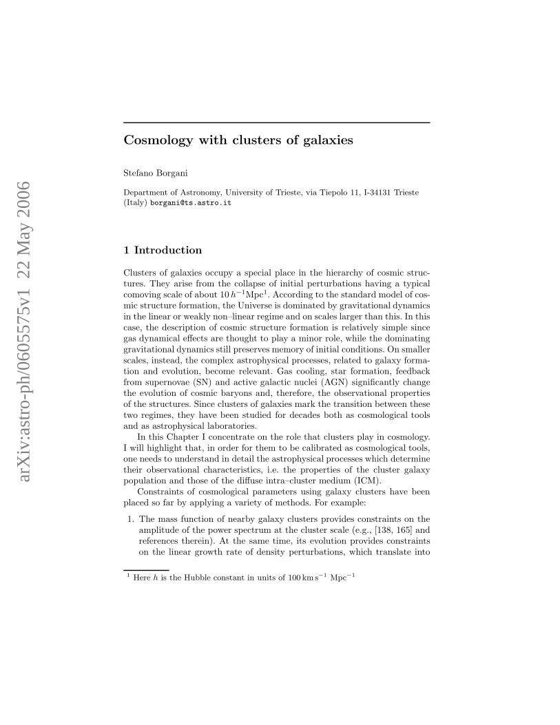
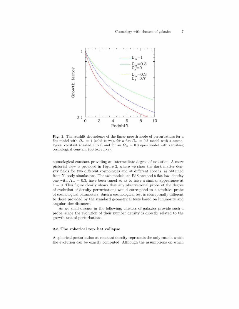
(e.g., [124]). I show in Figure 1 the redshift dependence of the linear growthfactor for an Eds model and for two models withΩm = 0.3 both with and with-out a cosmological constant term to restore spatial flatness. Quite apparently,the EdS has the faster evolution, while the slowing down of the perturba-tion growth is more apparent for the open low–density model, the presence of
Cosmology with clusters of galaxies 7
Fig. 1. The redshift dependence of the linear growth mode of perturbations for aflat model with Ωm = 1 (solid curve), for a flat Ωm = 0.3 model with a cosmo-logical constant (dashed curve) and for an Ωm = 0.3 open model with vanishingcosmological constant (dotted curve).
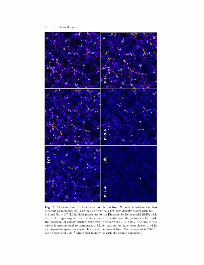
cosmological constant providing an intermediate degree of evolution. A morepictorial view is provided in Figure 2, where we show the dark matter den-sity fields for two different cosmologies and at different epochs, as obtainedfrom N–body simulations. The two models, an EdS one and a flat low–densityone with Ωm = 0.3, have been tuned so as to have a similar appearance atz = 0. This figure clearly shows that any observational probe of the degreeof evolution of density perturbations would correspond to a sensitive probeof cosmological parameters. Such a cosmological test is conceptually differentto those provided by the standard geometrical tests based on luminosity andangular–size distances.
As we shall discuss in the following, clusters of galaxies provide such aprobe, since the evolution of their number density is directly related to thegrowth rate of perturbations.
2.3 The spherical top–hat collapse
A spherical perturbation at constant density represents the only case in whichthe evolution can be exactly computed. Although the assumptions on which
8 Stefano Borgani
Fig. 2. The evolution of the cluster population from N–body simulations in twodifferent cosmologies [26]. Left panels describe a flat, low–density model with Ωm =0.3 and ΩΛ = 0.7 (L03); right panels are for an Einstein–de-Sitter model (EdS) withΩm = 1. Superimposed on the dark matter distribution, the yellow circles markthe positions of galaxy clusters with virial temperature T > 3 keV, the size of thecircles is proportional to temperature. Model parameters have been chosen to yielda comparable space density of clusters at the present time. Each snapshot is 250h−1
Mpc across and 75h−1 Mpc thick (comoving with the cosmic expansion).
Cosmology with clusters of galaxies 9
this model is based are quite restrictive, nevertheless it serves as a very use-ful guideline to characterize the process of evolution and formation of viri-alized DM halos. This approach is based on treating the perturbation as aseparate Friedmann–Lemaitre–Robertson–Walker (FLRW) universe, with theconstraint of null velocity at the boundary of the perturbation. Here we willsketch the derivation in the case of Ωm = 1 (e.g., [42], while an extension ofthis derivation to more general cosmologies can be found in [54] and [93], withuseful fitting functions provided in [31].
Assuming null velocities at an initial time ti provides the relationD+(ti) =(3/5)δ(ti), between the linear growth mode of the perturbation and the initialoverdensity. The initial density parameter, which characterizes this separateUniverse, is then Ωp(ti) = Ω(ti)(1 + δi). Therefore, the condition for theperturbation to recollapse will be Ωp(ti) > 1. If this condition is satisfied,then we can derive the density within the perturbation at the time tm of itsmaximum expansion (turn–around) as
ρp(tm) = ρc(ti)Ωp(ti)
[
Ωp(ti)− 1
Ωp(ti)
]3
. (16)
The time tm is given by the solution of the Friedmann equations for a closedUniverse:
tm =π
2Hi
Ωp(ti)
[Ωp(ti)− 1]3/2
=
[
3π
32Gρp(tm)
]
, (17)
where Hi is the Hubble parameter within the perturbation. At the same epochtm, the density of the general cosmic background is ρ(tm) = (6πGt2m)−1.Therefore, the exact value for the perturbation overdensity at the turn–aroundis
δ+(tm) =ρp(tm)
ρ(tm)− 1 =
(
3π
4
)2
− 1 ≃ 4.6 . (18)
On the other hand, the linear–theory extrapolation to tm would give
δ+(tm) = δ+(ti)
(
tmti
)2/3
=3
5
(
3π
4
)2/3
≃ 1.07 . (19)
This demonstrates that the linear–theory extrapolation significantly underes-timates overdensities at the turn-around.
After reaching the maximum expansion, the perturbation then evolves bydetaching from the general Hubble expansion and then recollapses, reachingvirial equilibrium supported by the velocity dispersion of DM particles. Thishappens at the virialization time tvir, at which the perturbation meets bydefinition the virial condition E = K+U = −K, being E, K and U the total,the kinetic and the potential energy, respectively.
At the turn–around point, the perturbation has no kinetic energy, so thatthe total energy is
10 Stefano Borgani
Em = U = −3
5
GM2
Rm, (20)
where we have used the expression for the potential energy of a uniform spher-ical density field of radius Rm and total mass M . In a similar manner, thetotal energy at the virialization is
Evir =U
2= −1
2
3
5
GM2
Rvir. (21)
Therefore, the condition of energy conservation in a dissipationless collapsegives Rm = 2Rvir for the relation between the radii at turn-around and atvirial equilibrium. This allows us to compute the overdensity at tvir as
ρp(tvir)
ρ(tvir)=
(
tvirtm
)2 (Rm
Rvir
)3ρp(tm)
ρ(tm)= 2223
(
3π
4
)2
= 18π2 ≃ 178 , (22)
where we have accounted for both the compression of the perturbation den-sity, due to its shrinking, and of the dilution of the background density asthe Universe expands from tm to tvir. Eq.(22) shows why an overdensity ofabout 200 is usually considered as typical for a DM halo which has reachedthe condition of virial equilibrium. As for the extrapolation of linear–theoryprediction, it would have given
δ+(tvir) =
(
tvirtm
)2/3
δ+(tm) ≃ 1.69 . (23)
The above equation shows the derivation of another fundamental number thatwill be used in what follows in order to characterize the mass function of viri-alized halos. It gives the overdensity that a perturbation in the initial densityfield must have for it to end up in a virialized structure. While the abovederivation holds for an EdS Universe, it can be generalized to any genericcosmology. For Ωm < 1 the increased expansion rate of the Universe causes afaster dilution of the cosmic density from tm to tvir and, as a consequence, alarger value of the overdensity at virialization.
In the following, we will indicate with ∆vir the overdensity at virial equi-librium, computed with respect to the background density, and with ∆c thesame quantity expressed in units of the critical density ρc. As a reference, aflat low–density model with Ωm = 0.3 has ∆c ≃ 100 and ∆vir ≃ 330. Also,we will use in the following the notation RN to indicate the radius of a haloencompassing an average overdensity equal to Nρc, so that MN will denotethe halo mass contained within that radius. As we shall see in the following,values often used in the literature are N = 200, 500 and 2500.
3 The mass function
The mass function (MF) at redshift z, n(M, z), is defined as the numberdensity of virialized halos found at that redshift with mass in the range
Cosmology with clusters of galaxies 11
[M,M + dM ]. In this section I will derive the MF expression following theapproach originally devised by Press and Schechter [132] (PS hereafter). Aftercommenting on the limitations of this approach, I will discuss the accuracywith which improved derivations of the MF reproduce the “exact” predictionsfrom N–body simulations.
3.1 The Press–Schechter mass function
The PS derivation of the MF is based on the assumption that the fraction ofmatter ending up in objects of a given mass M can be found by looking atthe portion of the initial (Lagrangian) density field, smoothed on the mass–scale M , lying at an overdensity exceeding a given critical threshold value,δc. Under the assumption of Gaussian perturbations, the probability for thelinearly–evolved smoothed field δM to exceed at redshift z the critical densitycontrast δc reads
p>δc(M, z) =1√
2πσM (z)
∫ ∞
δc
exp
(
− δ2M2σM (z)2
)
dδM =1
2erfc
(
δc√2σM (z)
)
,
(24)where erfc(x) is the complement error function and σM (z) = δ+(z)σM is thevariance at the mass scale M linearly extrapolated at redshift z. Under theassumption of spherical collapse, the critical overdensity δc is given by thelinear extrapolation of the overdensity at virial equilibrium, as derived in theprevious section. In this case, it will be δc = δc(z) with a weak dependenceupon redshift and cosmological parameters, with δc ≃ 1.69 independent ofz only in the case of an EdS cosmology. By definition, the above equationprovides the fraction of unity volume, which ends up by redshift z in objectswith mass above M . Therefore, the fraction of Lagrangian volume in objectswith mass in the range [M,M + dM ] is
dp>δc(M, z) =
∣
∣
∣
∣
∂p>δc(M, z)
∂M
∣
∣
∣
∣
dM . (25)
Since the probability of eq.(24) is a decreasing function of mass, the absolutevalue is required in order to have a positive–defined differential probability.Eq.(25) shows a fundamental limitation of the PS derivation of the MF. In-deed, we expect that, as we take the limit of arbitrarily small limiting mass,we should recover the whole mass content of the Universe. This is to say that,in the hierarchical clustering picture, all the mass is contained within halosof arbitrarily small mass. However, integrating eq.(25) over the whole massrange gives
∫∞
0 dp>δc(M, z) = 1/2. This implies that the PS derivation of themass function only accounts for half of the total mass at disposition. The basicreason for this is that, in this derivation, we give zero probability for a pointwith δM < δc, for a given filtering mass scale M , to have δM ′ > δc for somelarger filtering scale M ′ > M . This means that the PS approach neglects the
12 Stefano Borgani
possibility for that point to end up in a collapsed halo of larger mass. A morerigorous derivation of the mass function, which is based on the excursion–setformalism [23], correctly accounts for the missing factor 2, at least for the par-ticular choice of a sharp–k filter (i.e., a top–hat window function in Fourierspace).
Since eq.(25) provides the fraction of volume in objects of a given mass,the number density of such objects will be obtained after dividing it by thevolume, VM = M/ρ, occupied by each object. Therefore, after accounting forthe missing factor 2, the expression for the mass function reads
dn(M, z)
dM=
2
VM
∂p>δc(M, z)
∂M
=
√
2
π
ρ
M2
δcσM (z)
∣
∣
∣
∣
d log σM (z)
d logM
∣
∣
∣
∣
exp
(
− δ2c2σM (z)2
)
. (26)
This is the expression for the PS mass function. Although we will presentbelow a more accurate expressions for the MF, this equation already demon-strates the reason for which the mass function of galaxy clusters is a power-ful probe of cosmological models. Cosmological parameters enter in eq.(26)through the mass variance σM , which depends on the power spectrum and onthe cosmological density parameters, through the linear perturbation growthfactor, and, to a lesser degree, through the critical density contrast δc. Takingthis expression in the limit of massive objects (i.e., rich galaxy clusters), theMF shape is dominated by the exponential tail. This implies that the MF be-comes exponentially sensitive to the choice of the cosmological parameters. Inother words, a reliable observational determination of the MF of rich clusterswould allow us to place tight constraints on cosmological parameters.
3.2 Extensions of the PS approach and N–body tests
Following [89], an alternative way of recasting the mass function is
f(σM , z) =M
ρ
dn(M, z)
d lnσ−1M
. (27)
In this way, the PS expression is recovered by setting
f(σM , z) =
√
2
π
δcσM
exp
(
− δ2c2σ2
M
)
(28)
Despite its subtle simplicity (e.g., [112]), the PS MF has served for morethan a decade as a guide to constrain cosmological parameters from the massdistribution of galaxy clusters. Only with the advent of a new generation ofN–body simulations, which are able to cover a very large dynamical range,have significant deviations of the PS expression from the exact numerical
Cosmology with clusters of galaxies 13
description been noticed (e.g., [77, 76, 89, 59, 150, 166]). Such deviations havebeen usually interpreted in terms of corrections to the PS approach.
Incorporating the effect of non–spherical collapse, the PS expression hasbeen generalized [146] to
f(σM , z) =
√
2a
πC
[
1 +
(
σ2M
aδ2c
)q]δcσM
exp
(
− aδ2c2σ2
M
)
. (29)
These authors also compared this expression with results from N–body sim-ulations, in which the mass of the clusters were estimated with a sphericaloverdensity (SO) algorithm, by computing the mass within the radius encom-passing a mean overdensity equal to the virial one. As a result, they foundthe best–fitting values a = 0.707, q = 0.3, with the normalization constantC = 0.3222 obtained from the normalization requirement
∫∞
0f(σM )dν = 1
(note that the PS expression is recovered for a = 1, q = 0 and C = 1/2; seealso [147]).
Jenkins et al. [89] proposed an alternative expression for the mass function:
f(σM , z) = 0.315 exp(−| lnσ−1M + 0.61|3.8) , (30)
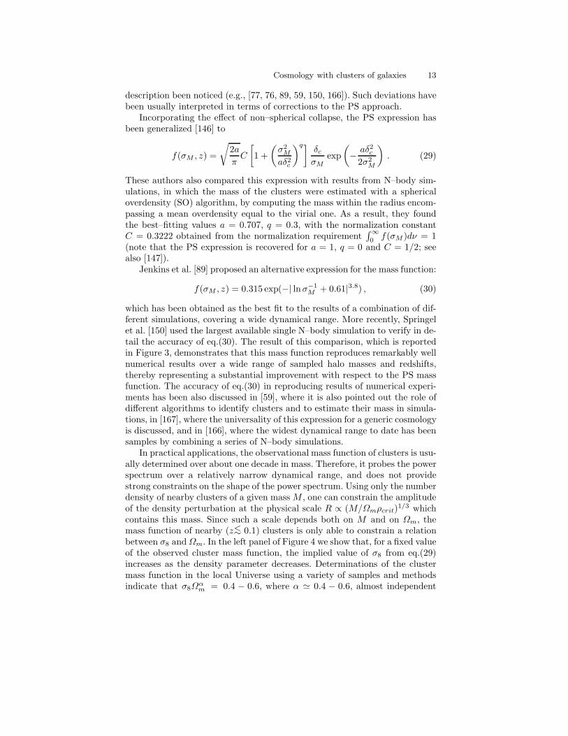
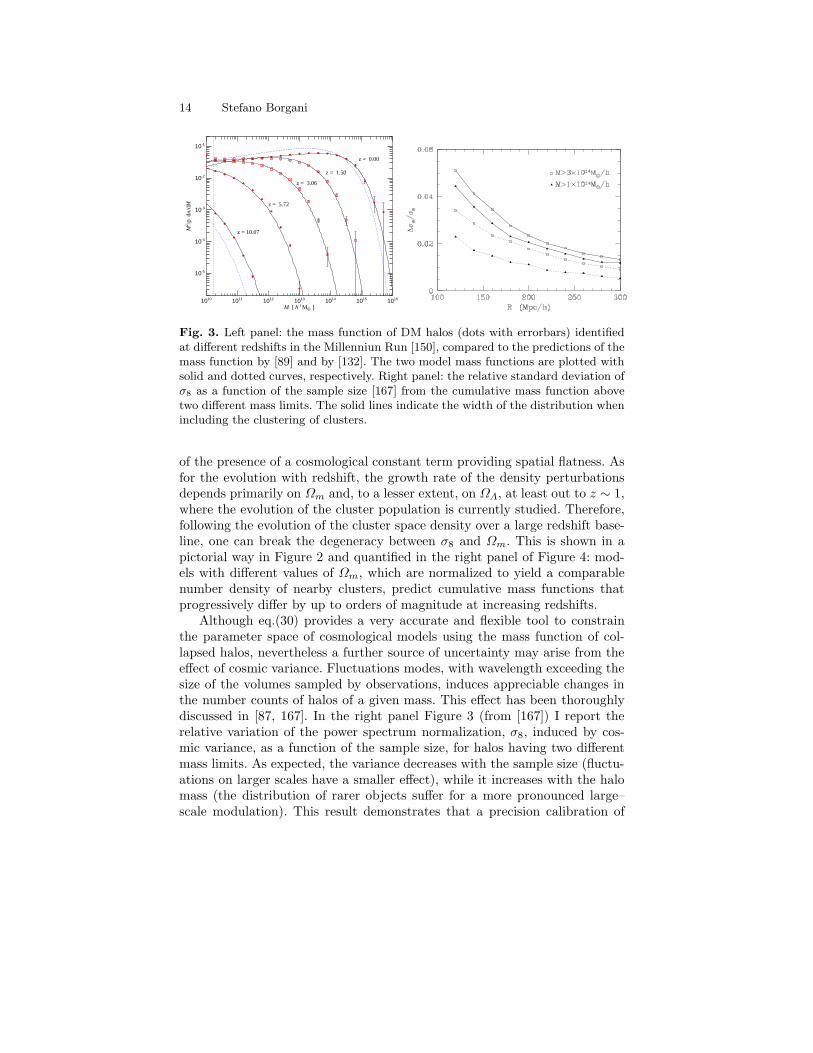
which has been obtained as the best fit to the results of a combination of dif-ferent simulations, covering a wide dynamical range. More recently, Springelet al. [150] used the largest available single N–body simulation to verify in de-tail the accuracy of eq.(30). The result of this comparison, which is reportedin Figure 3, demonstrates that this mass function reproduces remarkably wellnumerical results over a wide range of sampled halo masses and redshifts,thereby representing a substantial improvement with respect to the PS massfunction. The accuracy of eq.(30) in reproducing results of numerical experi-ments has been also discussed in [59], where it is also pointed out the role ofdifferent algorithms to identify clusters and to estimate their mass in simula-tions, in [167], where the universality of this expression for a generic cosmologyis discussed, and in [166], where the widest dynamical range to date has beensamples by combining a series of N–body simulations.
In practical applications, the observational mass function of clusters is usu-ally determined over about one decade in mass. Therefore, it probes the powerspectrum over a relatively narrow dynamical range, and does not providestrong constraints on the shape of the power spectrum. Using only the numberdensity of nearby clusters of a given mass M , one can constrain the amplitudeof the density perturbation at the physical scale R ∝ (M/Ωmρcrit)
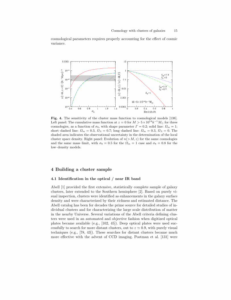
1/3 whichcontains this mass. Since such a scale depends both on M and on Ωm, themass function of nearby (z∼< 0.1) clusters is only able to constrain a relationbetween σ8 andΩm. In the left panel of Figure 4 we show that, for a fixed valueof the observed cluster mass function, the implied value of σ8 from eq.(29)increases as the density parameter decreases. Determinations of the clustermass function in the local Universe using a variety of samples and methodsindicate that σ8Ω
αm = 0.4 − 0.6, where α ≃ 0.4 − 0.6, almost independent
14 Stefano Borgani
1010 1011 1012 1013 1014 1015 1016
M [ h-1 MO • ]
10-5
10-4
10-3
10-2
10-1
M2 /ρ
dn/
dM
z = 10.07
z = 5.72
z = 3.06
z = 1.50
z = 0.00
Fig. 3. Left panel: the mass function of DM halos (dots with errorbars) identifiedat different redshifts in the Millenniun Run [150], compared to the predictions of themass function by [89] and by [132]. The two model mass functions are plotted withsolid and dotted curves, respectively. Right panel: the relative standard deviation ofσ8 as a function of the sample size [167] from the cumulative mass function abovetwo different mass limits. The solid lines indicate the width of the distribution whenincluding the clustering of clusters.
of the presence of a cosmological constant term providing spatial flatness. Asfor the evolution with redshift, the growth rate of the density perturbationsdepends primarily on Ωm and, to a lesser extent, on ΩΛ, at least out to z ∼ 1,where the evolution of the cluster population is currently studied. Therefore,following the evolution of the cluster space density over a large redshift base-line, one can break the degeneracy between σ8 and Ωm. This is shown in apictorial way in Figure 2 and quantified in the right panel of Figure 4: mod-els with different values of Ωm, which are normalized to yield a comparablenumber density of nearby clusters, predict cumulative mass functions thatprogressively differ by up to orders of magnitude at increasing redshifts.
Although eq.(30) provides a very accurate and flexible tool to constrainthe parameter space of cosmological models using the mass function of col-lapsed halos, nevertheless a further source of uncertainty may arise from theeffect of cosmic variance. Fluctuations modes, with wavelength exceeding thesize of the volumes sampled by observations, induces appreciable changes inthe number counts of halos of a given mass. This effect has been thoroughlydiscussed in [87, 167]. In the right panel Figure 3 (from [167]) I report therelative variation of the power spectrum normalization, σ8, induced by cos-mic variance, as a function of the sample size, for halos having two differentmass limits. As expected, the variance decreases with the sample size (fluctu-ations on larger scales have a smaller effect), while it increases with the halomass (the distribution of rarer objects suffer for a more pronounced large–scale modulation). This result demonstrates that a precision calibration of
Cosmology with clusters of galaxies 15
cosmological parameters requires properly accounting for the effect of cosmicvariance.
Fig. 4. The sensitivity of the cluster mass function to cosmological models [138].Left panel: The cumulative mass function at z = 0 for M > 5×10¹⁴h−1M⊙ for threecosmologies, as a function of σ8, with shape parameter Γ = 0.2; solid line: Ωm = 1;short–dashed line: Ωm = 0.3, ΩΛ = 0.7; long–dashed line: Ωm = 0.3, ΩΛ = 0. Theshaded area indicates the observational uncertainty in the determination of the localcluster space density. Right panel: Evolution of n(>M, z) for the same cosmologiesand the same mass–limit, with σ8 = 0.5 for the Ωm = 1 case and σ8 = 0.8 for thelow–density models.
4 Building a cluster sample
4.1 Identification in the optical / near IR band
Abell [1] provided the first extensive, statistically complete sample of galaxyclusters, later extended to the Southern hemisphere [2]. Based on purely vi-sual inspection, clusters were identified as enhancements in the galaxy surfacedensity and were characterized by their richness and estimated distance. TheAbell catalog has been for decades the prime source for detailed studies of in-dividual clusters and for characterizing the large scale distribution of matterin the nearby Universe. Several variations of the Abell criteria defining clus-ters were used in an automated and objective fashion when digitized opticalplates became available (e.g., [102, 45]). Deep optical plates were used suc-cessfully to search for more distant clusters, out to z ≃ 0.9, with purely visualtechniques (e.g., [78, 43]). These searches for distant clusters became muchmore effective with the advent of CCD imaging. Postman et al. [131] were
16 Stefano Borgani
the first to carry out a V&I-band survey over 5 deg2 (the Palomar DistantCluster Survey, PDCS). This technique enhances the contrast of galaxy over-density at a given position, utilizing prior knowledge of the luminosity profiletypical of galaxy clusters. Dalcanton [44] proposed another method of opticalselection of clusters, in which drift scan imaging data from relatively smalltelescopes is used to detect clusters as positive surface brightness fluctuationsin the background sky. Gonzalez et al. [75] applied a technique based on sur-face brightness fluctuations from drift scan imaging data to build a sample of∼1000 cluster candidates over 130 deg2.
A common feature of all these methods of cluster identification is that theyclassify clusters according to definitions of richness, which generally have aloose relation with the actual cluster mass. This represents a serious limitationfor any cosmological application, which requires the observable, on which thecluster selection is based, to be a reliable proxy of the cluster mass.
An improved definition of richness, based on the amplitude of the galaxy–cluster cross–correlation function, has been applied [74] to clusters identified ina large area survey in R and z bands (the Red Sequence Cluster Survey). Thissurvey, whose optical and X–ray follow–up, is currently underway, promisesto unveil a fairly large number of clusters out to z ∼ 1.5.
By increasing the number of observed passbands and using red colors onecan increase the contrast with which clusters are seen in color space. In thisway, one can increase the efficiency of cluster selection also at high redshift(e.g., [151, 74, 152]) and the accuracy of their estimated redshifts throughspectro–photometric techniques. In this way, Miller et al. [111] designed acluster–finding algorithm which makes full use of information of both posi-tion and color space to detect clusters of galaxies from the SDSS. They wereable to identify about 750 clusters out to z∼< 0.2, and assessed the degree ofcompleteness by resorting to a comparison with mock SDSS surveys extractedfrom large N–body simulations. Once completed, the search of clusters overthe entire SDSS sample will provide about 2500 nearby and medium–distantobjects. At the same time the next generation of wide field (> 100 deg2)deep multicolor surveys in the optical and especially the near-infrared willpowerfully enhance the search for distant clusters, out to z∼> 1.
4.2 Identification in the X–ray band
Already from the first pioneering attempts to map the X–ray sky ([66],see [138] for a historical review), clusters were associated with extendedsources, whose dominant emission mechanism was recognized to be thermalbremsstrahlung from optically thin plasma at a temperature of several keV[61, 40]. The all–sky survey conducted by the the HEAO-1 X-ray Observatorywas the first to provide a flux–limited sample of X–ray identified clusters, forwhich both the flux number counts and the X–ray luminosity function havebeen computed for the first time [126]. However, it is only thanks to the muchimproved sensitivity of the Einstein Observatory [65] that X-ray surveys were
Cosmology with clusters of galaxies 17
recognized as an efficient means of constructing samples of galaxy clusters outto cosmologically interesting redshifts.
First, the X-ray selection has the advantage of revealing physically-boundsystems, because diffuse emission from a hot ICM is the direct manifestationof the existence of a potential-well within which the gas is in dynamical equi-librium with the cool baryonic matter (galaxies) and the dark matter. Second,the X-ray luminosity is well correlated with the cluster mass (see Figure 11).Third, the X-ray emissivity is proportional to the square of the gas density,hence cluster emission is more concentrated than the optical bidimensionalgalaxy distribution. In combination with the relatively low surface densityof X-ray sources, this property makes clusters high contrast objects in theX-ray sky, and alleviates problems due to projection effects that affect opti-cal selection. Finally, an inherent fundamental advantage of X-ray selection isthe ability to define flux-limited samples with well-understood selection func-tions. This leads to a simple evaluation of the survey volume and thereforeto a straightforward computation of space densities. Nonetheless, there aresome important caveats described below. Pioneering work in this field [67, 84]was based on the Einstein Observatory Extended Medium Sensitivity Survey(EMSS). The EMSS survey covered over 700 square degrees and lead to theconstruction of a flux-limited sample of 93 clusters out to z = 0.58, allowingthe cosmological evolution of clusters to be investigated.
The ROSAT satellite, launched in 1990, allowed a significant step for-ward in X-ray surveys of clusters. The ROSAT All-Sky Survey (RASS, [156])was the first X-ray imaging mission to cover the entire sky, thus paving theway to large contiguous-area surveys of X-ray selected nearby clusters. In thenorthern hemisphere, the largest compilations with virtually complete opticalidentification include, the Bright Cluster Sample (BCS, [51]), and the North-ern ROSAT All Sky Survey (NORAS, [22]). In the southern hemisphere, theROSAT-ESO flux limited X-ray (REFLEX) cluster survey [21] has completedthe identification of 452 clusters, the largest, homogeneous compilation todate. The Massive Cluster Survey (MACS, [52]) is aimed at targeting themost luminous systems at z > 0.3 which can be identified in the RASS at thefaintest flux levels. The deepest area in the RASS, the North Ecliptic Pole(NEP, [85]) which ROSAT scanned repeatedly during its All-Sky survey, wasused to carry out a complete optical identification of X-ray sources over a 81deg2 region. This study yielded 64 clusters out to redshift z = 0.81.
In total, surveys covering more than 104 deg2 have yielded over 1000 clus-ters, out to redshift z ≃ 0.5. A large fraction of these are new discoveries,whereas approximately one third are identified as clusters in the Abell orZwicky catalogs. For the homogeneity of their selection and the high degreeof completeness of their spectroscopic identifications, these samples are nowthe basis for a large number of follow-up investigations and cosmological stud-ies.
Besides the all-sky surveys, the ROSAT-PSPC archival pointed obser-vations were intensively used for serendipitous searches of distant clusters.

18 Stefano Borgani
These projects, which are now completed, include: the RIXOS survey [38],the ROSAT Deep Cluster Survey (RDCS, [139, 138]), the Serendipitous High-Redshift Archival ROSAT Cluster survey (SHARC, [32], the Wide AngleROSAT Pointed X-ray Survey of clusters (WARPS, [125]), the 160 deg2 largearea survey [117], the ROSAT Optical X-ray Survey (ROXS, [49]). ROSAT-HRI pointed observations have also been used to search for distant clusters inthe Brera Multi-scale Wavelet catalog (BMW, [113]).
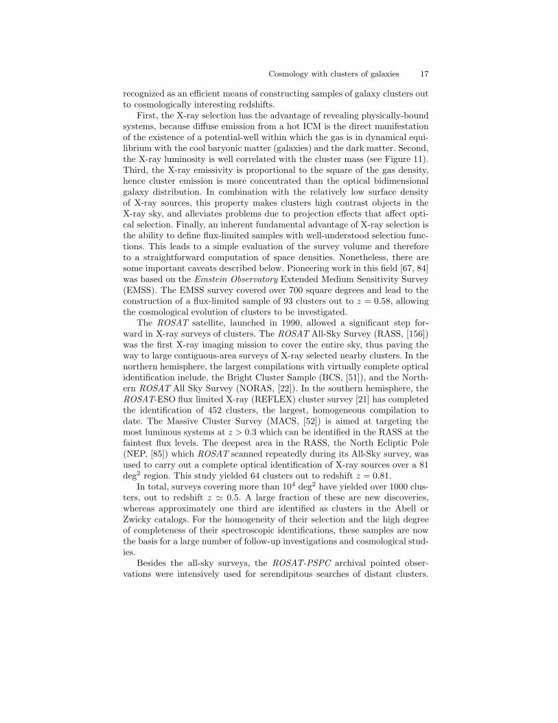
Fig. 5. Solid angles and flux limits of X-ray cluster surveys carried out over the lasttwo decades. Dark filled circles represent serendipitous surveys constructed from acollection of pointed observations. Light shaded circles represent surveys coveringcontiguous areas. The hatched region is a predicted locus of current serendipitoussurveys with Chandra and Newton-XMM. From [138].
In Figure 5, we give an overview of the flux limits and surveyed areas ofall major cluster surveys carried out over the last two decades. RASS-basedsurveys have the advantage of covering contiguous regions of the sky so thatthe clustering properties of clusters (e.g., [143]) can be investigated. They
Cosmology with clusters of galaxies 19
also have the ability to unveil rare, massive systems albeit over a limitedredshift and X-ray luminosity range. Serendipitous surveys which are at leasta factor of ten deeper but cover only a few hundreds square degrees, providecomplementary information on lower luminosities, more common systems andare well suited for studying cluster evolution on a larger redshift baseline.
A number of systematic studies have been carried out to compare thenature of clusters identified with the optical and the X–ray technique (e.g.,[48, 13, 129]). The general conclusion of these studies is that optically selectedclusters are on average underluminous in the X-ray band. This suggests thatoptical selection tends to pick up objects which have not yet reached a highenough density to make the ICM lighting up in X–rays.
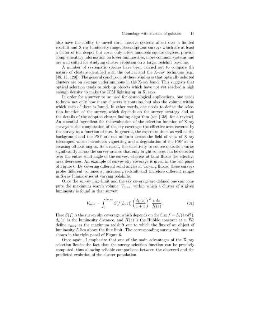
In order for a survey to be used for cosmological applications, one needsto know not only how many clusters it contains, but also the volume withinwhich each of them is found. In other words, one needs to define the selec-tion function of the survey, which depends on the survey strategy and onthe details of the adopted cluster finding algorithm (see [138], for a review).An essential ingredient for the evaluation of the selection function of X-raysurveys is the computation of the sky coverage: the effective area covered bythe survey as a function of flux. In general, the exposure time, as well as thebackground and the PSF are not uniform across the field of view of X-raytelescopes, which introduces vignetting and a degradation of the PSF at in-creasing off-axis angles. As a result, the sensitivity to source detection variessignificantly across the survey area so that only bright sources can be detectedover the entire solid angle of the survey, whereas at faint fluxes the effectivearea decreases. An example of survey sky coverage is given in the left panelof Figure 6. By covering different solid angles at varying fluxes, these surveysprobe different volumes at increasing redshift and therefore different rangesin X-ray luminosities at varying redshifts.
Once the survey flux–limit and the sky coverage are defined one can com-pute the maximum search volume, Vmax, within which a cluster of a givenluminosity is found in that survey:
Vmax =
∫ zmax
0
S[f(L, z)]
(
dL(z)
1 + z
)2c dz
H(z). (31)
Here S(f) is the survey sky coverage, which depends on the flux f = L/(4πd2L),dL(z) is the luminosity distance, and H(z) is the Hubble constant at z. Wedefine zmax as the maximum redshift out to which the flux of an object ofluminosity L lies above the flux limit. The corresponding survey volumes areshown in the right panel of Figure 6.
Once again, I emphasize that one of the main advantages of the X–rayselection lies in the fact that the survey selection function can be preciselycomputed, thus allowing reliable comparisons between the observed and thepredicted evolution of the cluster population.
20 Stefano Borgani
Fig. 6. Left panel: sky coverage as a function of X-ray flux of several serendipitoussurveys. Right panel: corresponding search volumes, V (> z), for a cluster of givenX-ray luminosity (LX = 3× 1044 [0.5− 2 keV] ≃ L∗
X). From [138].
4.3 Identification through the SZ effect
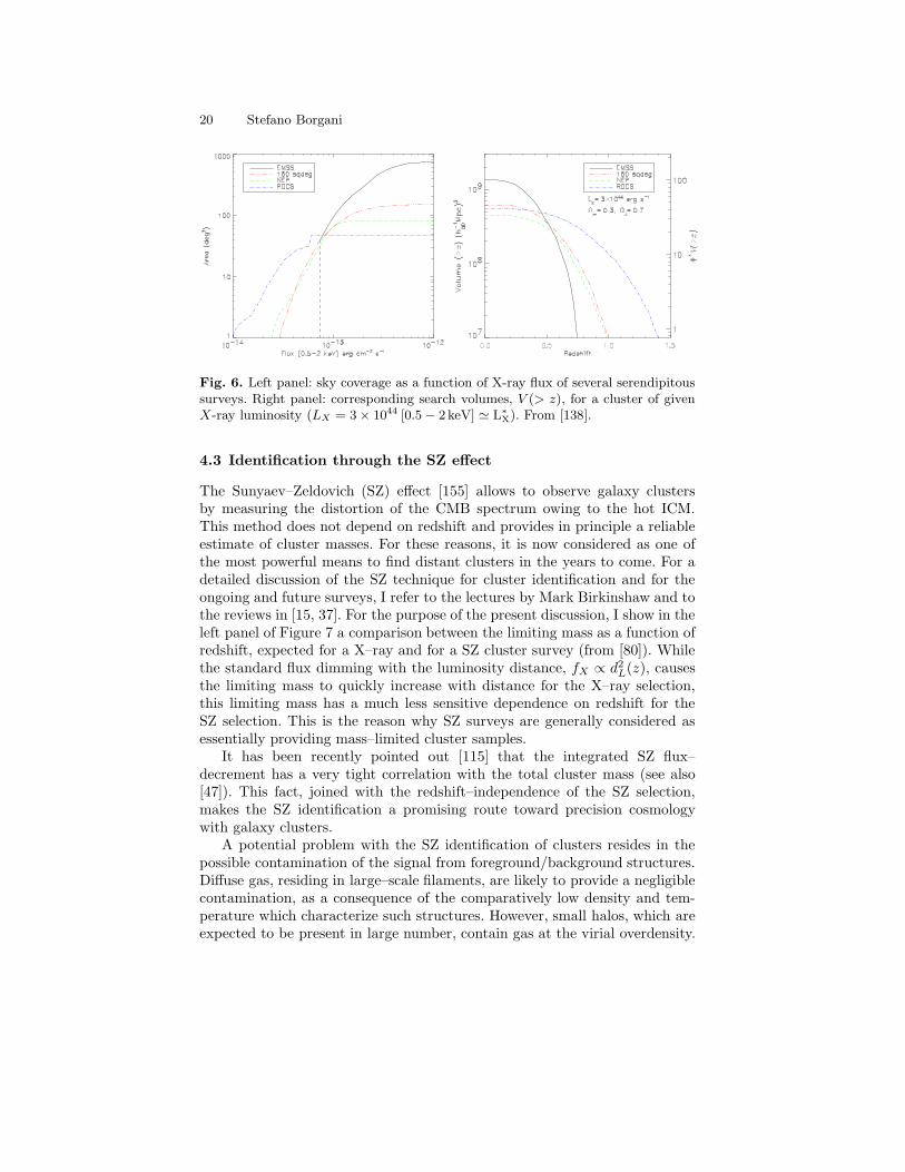
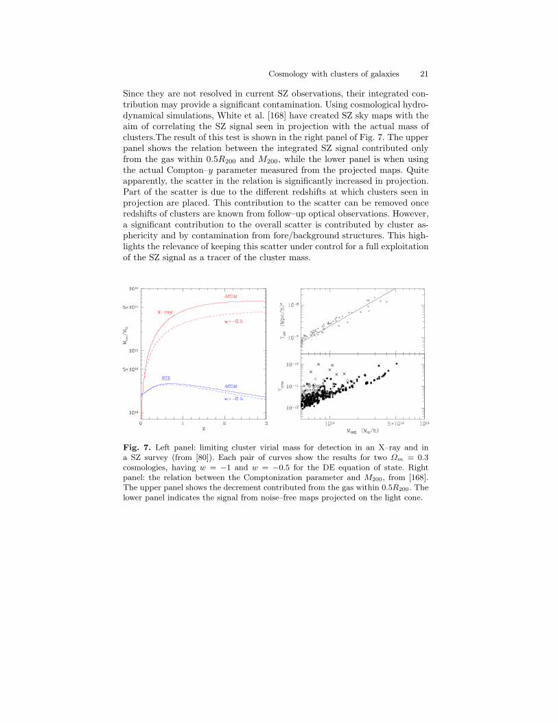
The Sunyaev–Zeldovich (SZ) effect [155] allows to observe galaxy clustersby measuring the distortion of the CMB spectrum owing to the hot ICM.This method does not depend on redshift and provides in principle a reliableestimate of cluster masses. For these reasons, it is now considered as one ofthe most powerful means to find distant clusters in the years to come. For adetailed discussion of the SZ technique for cluster identification and for theongoing and future surveys, I refer to the lectures by Mark Birkinshaw and tothe reviews in [15, 37]. For the purpose of the present discussion, I show in theleft panel of Figure 7 a comparison between the limiting mass as a function ofredshift, expected for a X–ray and for a SZ cluster survey (from [80]). Whilethe standard flux dimming with the luminosity distance, fX ∝ d2L(z), causesthe limiting mass to quickly increase with distance for the X–ray selection,this limiting mass has a much less sensitive dependence on redshift for theSZ selection. This is the reason why SZ surveys are generally considered asessentially providing mass–limited cluster samples.
It has been recently pointed out [115] that the integrated SZ flux–decrement has a very tight correlation with the total cluster mass (see also[47]). This fact, joined with the redshift–independence of the SZ selection,makes the SZ identification a promising route toward precision cosmologywith galaxy clusters.
A potential problem with the SZ identification of clusters resides in thepossible contamination of the signal from foreground/background structures.Diffuse gas, residing in large–scale filaments, are likely to provide a negligiblecontamination, as a consequence of the comparatively low density and tem-perature which characterize such structures. However, small halos, which areexpected to be present in large number, contain gas at the virial overdensity.
Cosmology with clusters of galaxies 21
Since they are not resolved in current SZ observations, their integrated con-tribution may provide a significant contamination. Using cosmological hydro-dynamical simulations, White et al. [168] have created SZ sky maps with theaim of correlating the SZ signal seen in projection with the actual mass ofclusters.The result of this test is shown in the right panel of Fig. 7. The upperpanel shows the relation between the integrated SZ signal contributed onlyfrom the gas within 0.5R200 and M200, while the lower panel is when usingthe actual Compton–y parameter measured from the projected maps. Quiteapparently, the scatter in the relation is significantly increased in projection.Part of the scatter is due to the different redshifts at which clusters seen inprojection are placed. This contribution to the scatter can be removed onceredshifts of clusters are known from follow–up optical observations. However,a significant contribution to the overall scatter is contributed by cluster as-phericity and by contamination from fore/background structures. This high-lights the relevance of keeping this scatter under control for a full exploitationof the SZ signal as a tracer of the cluster mass.
Fig. 7. Left panel: limiting cluster virial mass for detection in an X–ray and ina SZ survey (from [80]). Each pair of curves show the results for two Ωm = 0.3cosmologies, having w = −1 and w = −0.5 for the DE equation of state. Rightpanel: the relation between the Comptonization parameter and M200, from [168].The upper panel shows the decrement contributed from the gas within 0.5R200 . Thelower panel indicates the signal from noise–free maps projected on the light cone.
22 Stefano Borgani
5 Methods to estimate cluster masses
5.1 The hydrostatic equilibrium
The condition of hydrostatic equilibrium determines the balance between thepressure force and the gravitational force: ∇Pgas = −ρgas∇φ, where Pgas andρgas are the gas pressure and density, respectively, while φ is the underlyinggravitational potential. Under the assumption of a spherically symmetric gasdistribution, the above equations read:
dPgas
dr= −ρgas
dφ
dr= −ρgas
GM(< r)
r2, (32)
where r is the radial coordinate (clustercentric distance) and M(< r) is thetotal mass contained within r. Using the equation of state of ideal gas to relatepressure to gas density and temperature, the mass is then given by
M(< r) = − r
G
kBT
µmp
(
d ln ρgasd ln r
+d lnT
d ln r
)
, (33)
where µ is the mean molecular weight of the gas (µ ≃ 0.59 for primordialcomposition) and mp is the proton mass. An often used mass estimator isbased on assuming the β–model for the gas density profile,
ρgas(r) =ρ0
[1 + (r/rc)2]3β/2
(34)
[39]. In the above equation, rc is the core radius, while β is the ratio betweenthe kinetic energy of any tracer of the gravitational potential (e.g. galaxies)and the thermal energy of the gas, β = µmpσ
2v/(kBT ) (σv: one–dimensional
velocity dispersion). By further assuming a polytropic equation of state, ρgas ∝P γgas (γ: polytropic index), eq.(33) becomes
M(< r) ≃ 1.11× 10¹⁴βγT (r)
keV
r
h−1Mpc
(r/rc)2
1 + (r/rc)2h−1M⊙ , (35)
where T (r) is the temperature at the radius r. In its original derivation, theβ–model was aimed at representing the distribution of isothermal gas sittingin hydrostatic equilibrium within a King–like potential. The correspondingmass estimator is recovered from eq.(35) by setting γ = 1 and replacing T (r)with the global ICM temperature, T0. In the absence of accurately resolvedtemperature profiles from X–ray observations, eq.(35) has been used to esti-mate cluster masses both in its isothermal (e.g., [136]) and in its polytropicform (e.g., [120, 62, 56]).
Thanks to the much improved sensitivity of the Chandra and XMM–Newton X–ray observatories, temperature profiles are now resolved with highenough accuracy to allow the application of more general methods of mass
Cosmology with clusters of galaxies 23
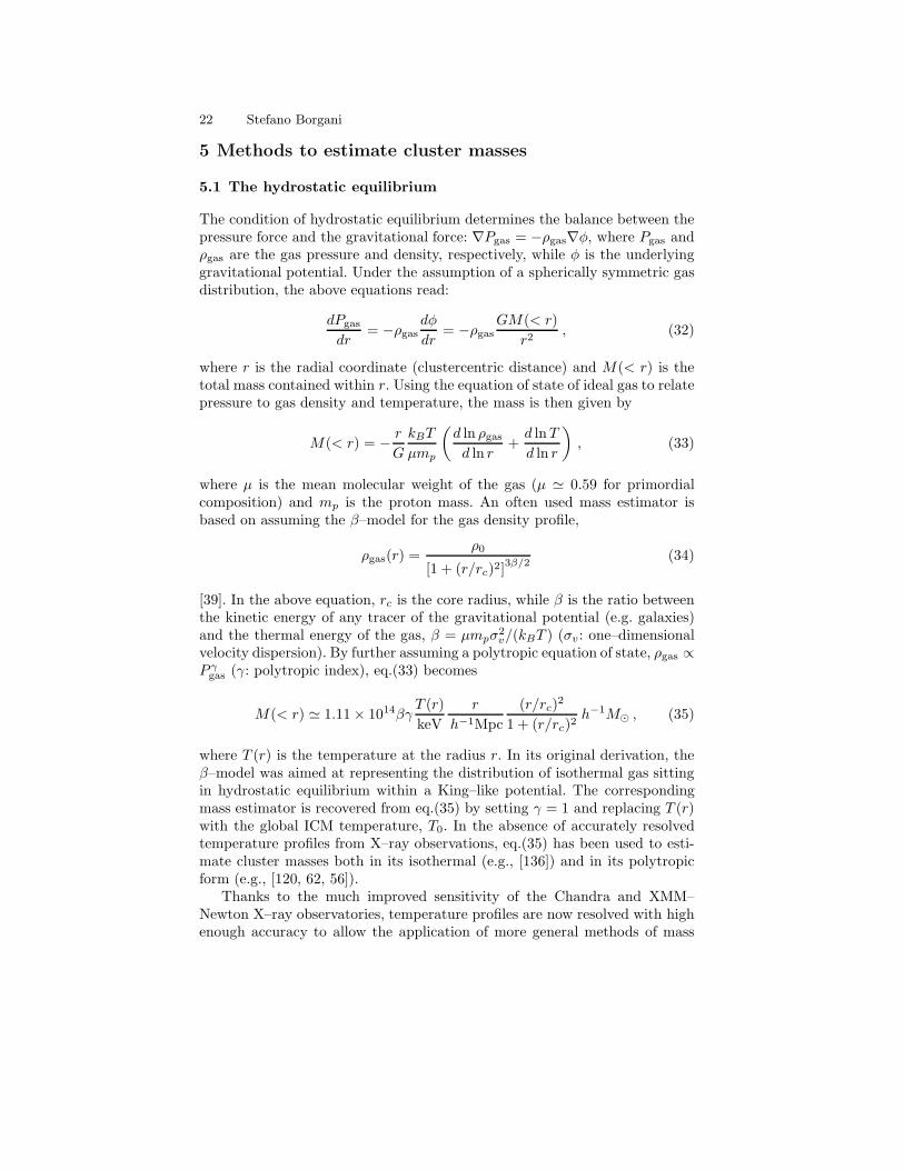
Fig. 8. The mass-temperature relation for nearby clusters (from [8]) and for distantclusters (from [95]), based on a combination of Chandra and XMM–Newton data.
estimation, not necessarily bound to the assumptions of β–model and of anoverall polytropic form for the equation of state (e.g., [5, 56, 8, 161]).
An alternative way of recasting the isothermal version of eq.(35) betweentemperature and mass is based on expressing the mass according to the virialtheorem as Mvir = σ2
vRvir/G, so that
kBT =1.38
β
(
Mvir
1015 h−1M⊙
)3/2
[Ωm∆vir(z)]1/3 (1 + z) keV . (36)
This expression, originally introduced in [54], has been sometimes used toexpress the M–T relation as obtained from hydrodynamical simulations ofgalaxy clusters (e.g., [31, 25]).
It is clear that the two crucial assumptions underlying any mass measure-ments based on the ICM temperature concerns the existence of hydrostaticequilibrium and of spherical symmetry. While effects of non–spherical geome-try can be averaged out by performing the analysis over a large enough numberof clusters, the former can lead to systematic biases in the mass estimates (e.g.,[133]) and references therein). So far, ICM temperature measurements havebeen based on fits of the observed X–ray spectra of clusters to plasma models,which are dominated at high temperatures by thermal bremsstrahlung. How-ever, local deviations from isothermality, e.g. due to the presence of mergingcold gas clumps, can bias the spectroscopic temperature with respect to theactual electron temperature (e.g., [108, 110, 160]). This bias directly translatesinto a comparable bias in the mass estimate through hydrostatic equilibrium(see Section 7, below).
24 Stefano Borgani
5.2 The dynamics of member galaxies
From a historical point of view, the dynamics traced by member galaxies, hasbeen the first method applied to measure masses of galaxy clusters [148, 172].Under the assumption of virial equilibrium, the mass of the cluster can beestimated by knowing position and redshift for a high enough number ofmember galaxies:
M =π
2
3σ2vRV
G(37)
(e.g., [99]), where the first factor accounts for the geometry of projection,σr is the line-of-sight velocity dispersion and RV is the virialization radius,which depends on the positions of the galaxies with measured redshifts andrecognized as true cluster members:
RV = N2
∑
i>j
r−1ij
−1
, (38)
where N is the total number of galaxies, and rij the projected separationbetween the i-th and j-th galaxies. This method has been extensively appliedto measure masses for statistical samples of both nearby (e.g., [17, 71, 16, 137,130]) and distant (e.g., [36, 73]) clusters.
Besides the assumption of virial equilibrium, which may be fulfilled to dif-ferent degrees by different populations of galaxies (e.g., late vs. early type),a crucial aspect in the application of the dynamical mass estimator concernsthe rejection of interlopers, i.e. of back/foreground galaxies which lie alongthe line-of-sight of the cluster without belonging to it. A spurious inclusionof non–member galaxies in the analysis leads in general to an overestimate ofthe velocity dispersion and, therefore, of the resulting mass. A number of al-gorithms have been developed for interlopers rejection, whose reliability mustbe judged on a case-by-case basis (e.g., [68, 157]). A further potential prob-lem of this analysis concerns the possibility of realizing a uniform samplingof the cluster potential using galaxies with measured redshifts. For instance,the technical difficulty of packing slits or fibers in optical spectroscopic obser-vations may lead to an undersampling of the cluster central regions. In turn,this leads to an overestimate of RV and, again, of the collapsed mass.
Tests of the accuracy of mess estimates based on the dynamical virialmethod have been performed by using hydrodynamical simulations of galaxyclusters, in which galaxies are identified from gas cooling and star formation([63, 18]). For instance, [18] have shown that galaxies identified in the simu-lations are fair tracers of the underlying dynamics, with no systematic bias inthe estimate of cluster masses, although a rather large scatter between trueand recovered masses is induced mostly by projection effects.
Quite reassuringly, despite all the assumptions and possible systematicsaffecting both dynamical optical and X–ray mass estimates, these two methods
Cosmology with clusters of galaxies 25
0 5 10 15
1
2
3
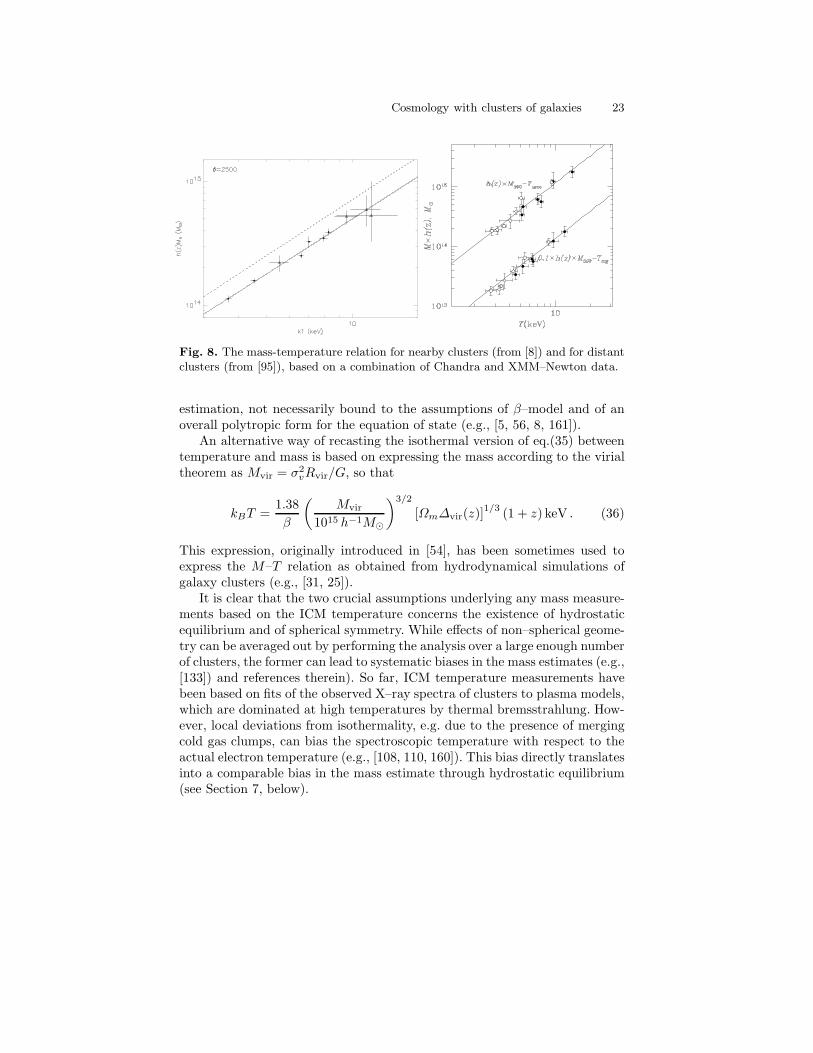
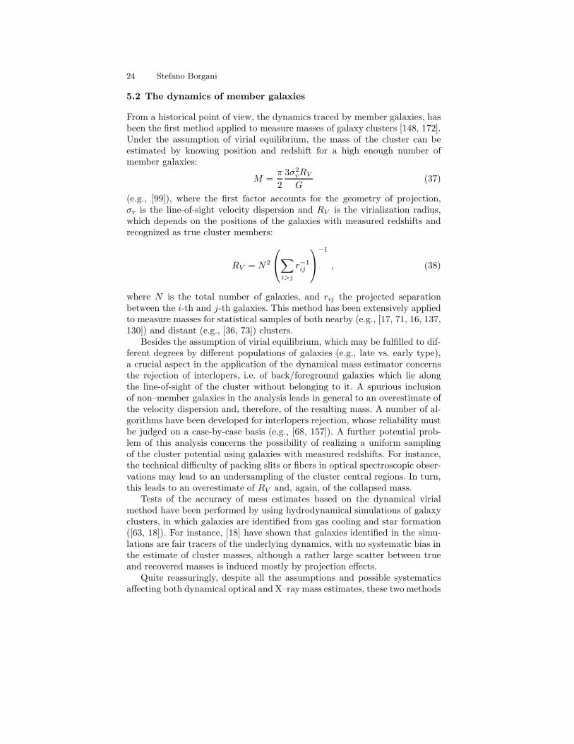
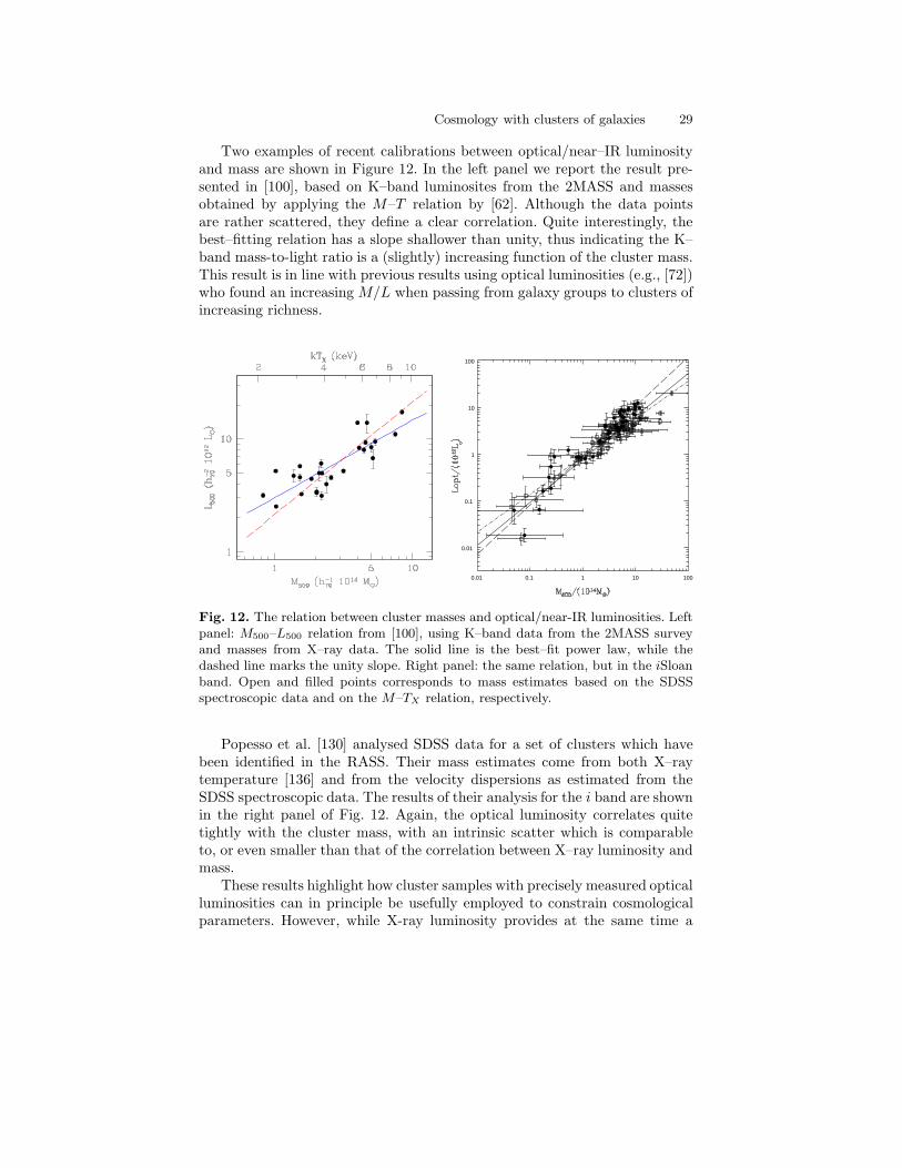
Fig. 9. The relation between dynamical optical masses and masses derived fromthe X–ray temperature by assuming hydrostatic equilibrium (from [71], left panel,and from [130], right panel, based on SDSS spectroscopic data).
provide in general fairly consistent results for both nearby (e.g., [71, 130])and distant (e.g., [96]) clusters. Two examples of such comparisons are shownin Figure 9. In the left panel, we report the comparison between X–ray andoptical dynamical masses [71]. This plot shows a reasonable agreement amongthe two mass estimates, although with some scatter. The right panel reportsthe comparison presented in [130]. In this plot, the triangles indicates thecluster with clear evidences of complex dynamics. Quite interestingly, theagreement between the two mass estimates is acceptable, with a few outlierswhich are generally identified with non–relaxed clusters.
5.3 The self–similar scaling
The simplest model to explain the physics of the ICM is based on the assump-tion that gravity only determines the thermodynamical properties of the hotdiffuse gas [90]. Since gravity does not have a preferred scale, we expect clus-ters of different sizes to be the scaled version of each other as long as gravityonly determines the ICM evolution and there are no preferred scales in theunderlying cosmological model. This is the reason why the ICM model basedon the effect of gravity only is said to be self-similar.
If we define M∆cas the mass contained within the radius R∆c
, encompass-ing a mean density ∆c times the critical density, then M∆c
∝ ρc(z)∆cR3∆c
.Here ρc(z) is the critical density of the universe which scales with redshift asρc(z) = ρc,0E
2(z), where E(z) is given by eq.(12). On the other hand, thecluster size R scales with z and M∆c
as R ∝ M1/3E−2/3(z). Therefore, as-suming hydrostatic equilibrium, the cluster mass scales with the temperature
26 Stefano Borgani
T asM∆c
∝ T 3/2E−1(z) . (39)
If ρgas is the gas density, the corresponding X–ray luminosity for pure thermalbremsstrahlung emission is
LX =
∫
V
(
ρgasµmp
)2
Λ(T ) dV , (40)
where Λ(T ) ∝ T 1/2. Further assuming that the gas distribution traces thedark matter distribution, ρgas(r) ∝ ρDM (r), then
LX ∝ M∆cρcT
1/2 ∝ T 2E(z) . (41)
As for the CMB intensity decrement due to the thermal SZ effect we have
∆S ∝∫
y(θ)dΩ ∝ d−2A
∫
Tned3r ∝ d−2
A T 5/2E−1(z) , (42)
where y is the Comptonization parameter, dA is the angular size distance andne is the electron number density. We can also write ∆S in a different way toget the explicit dependence on y0:
∆S ∝ y0d−2A
∫
dΩ ∝ y0d−2A M2/3E−4/3(z) ∝ y0d
−2A TE−2(z) . (43)
In this way, we obtain the following scalings for the central value of the Comp-tonization parameter:
y0 ∝ T 3/2E(z) ∝ L3/4X E1/4(z) . (44)
Eqs.(39), (41) and (44) are unique predictions for the scaling relationsamong ICM physical quantities and, in principle, they provide a way to relatethe cluster masses to observables at different redshifts. As we shall discuss inthe following, deviations with respect to these relations witness the presence ofmore complex physical processes, beyond gravitational dynamics only, whichaffect the thermodynamical properties of the diffuse baryons and, therefore,the relation between observables and cluster masses.
5.4 Phenomenological scaling relations
Using the X–ray luminosity
The relation between X–ray luminosity and temperature of nearby clustersis considered as one of the most robust observational facts against the self–similar model of the ICM. A number of observational determinations nowexist, pointing toward a relation LX ∝ Tα, with α ≃ 2.5–3 (e.g., [171]), pos-sibly flattening towards the self–similar scaling only for the very hot systems
Cosmology with clusters of galaxies 27
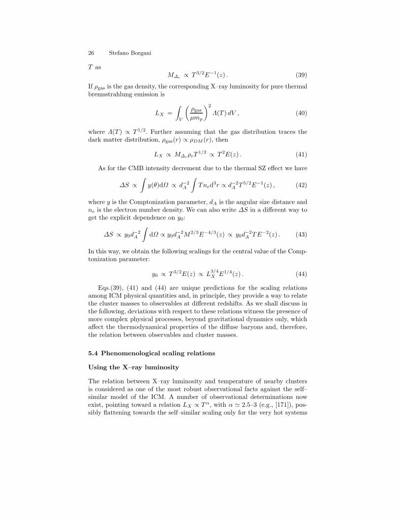
with T∼> 10 keV [3]. While in general the scatter around the best–fitting re-lation is non negligible, it has been shown to be significantly reduced afterexcising the contribution to the luminosity from the cluster cooling regions[106] or by removing from the sample clusters with evidence of cooling flows[7]. As for the behaviour of this relation at the scale of groups, T∼< 1 keV, theemerging picture now is that it lies on the extension of the LX–T relation ofclusters, with no evidence for a steepening [116], although with a significantincrease of the scatter [121], possibly caused by a larger diversity of the groupspopulation when compared to the cluster population. This result is reportedin the left panel of Figure 10 (from [121]), which shows the LX–T relation fora set of clusters with measured ASCA temperatures and for a set of groups.
-0.5 0 0.5 1
42
44
46
0.5
1
1.5
2
2.5
3
3.5
0 0.2 0.4 0.6 0.8 1 1.2 1.4
L/T
B
z
(1+z)1.2
E(z)(∆v(z)/∆v(0))1/2
E(z)t(0)/(E(z)t(z)) - cooling thresholdt(0)2/(E(z)3t(z)2) - altered similarity binned data compared with AE99 binned data compared with Markevitch (1998)
Fig. 10. Left panel: the LX–T relation for nearby clusters and groups (from [121]).The star symbols are the for the sample of clusters, with temperature measured fromASCA, while the filled squares and open circles are for a sample of groups, also withASCA temperatures. Right panel: the evolution of the LX–T relation, normalizedto the local relation (from [109]), using Chandra temperatures of clusters at z > 0.4.
As for the evolution of the LX–T relation, a number of analyses have beenperformed, using Chandra [86, 162, 57, 109] and XMM–Newton [95, 101] data.Although some differences exist between the results obtained from differentauthors, such differences are most likely due to the convention adopted forthe radii within which luminosity and temperature are estimated. In general,the emerging picture is that clusters at high redshift are relatively brighter,at fixed temperature. The resulting evolution for a cosmology with Ωm = 0.3and ΩΛ = 0.7 is consistent with the predictions of the self–similar scaling,although the slope of the high–z LX–T relation is steeper than predicted byself–similar scaling, in keeping with results for nearby clusters. The left panelof Fig. 10 shows the evolution of the LX–T relation from [109], where Chandraand XMM–Newton observations of 11 clusters with redshift 0.6 < z < 1.0were analyzed. The vertical axis reports the quantity LX/TB, where B is theslope of the local relation. Quite apparently, distant clusters are systematicallybrighter relatively to the local ones. However, the uncertainties are still large
28 Stefano Borgani
enough not to allow the determination of a precise redshift dependence of theLX–T normalization.
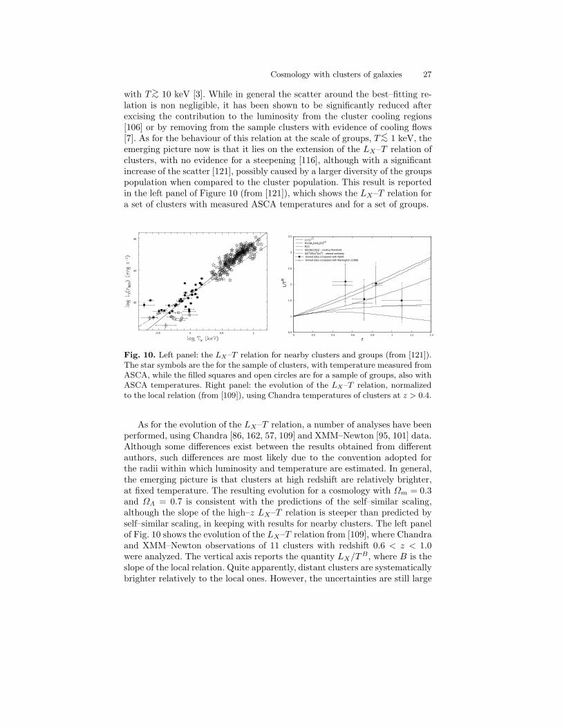
As for the relation between X–ray luminosity and mass, its first calibrationhas been presented in [136], for a sample of bright clusters extracted fromthe ROSAT All Sky Survey (RASS). In their analysis, these authors derivedmasses by using temperatures derived from ASCA observations and applyingthe equation of hydrostatic equilibrium, eq.(33), for an isothermal β–model.The resulting M–LX relation is shown in Figure 11. From the one hand, thisrelation demonstrates that a well defined relation between X–ray luminosityand mass indeed exist, although with some scatter, thus confirming that LX
can indeed be used as a proxy of the cluster mass. From the other hand, theslope of the relation is found to be steeper than the self–similar scaling, thusconsistent with the observed LX–T relation.
Fig. 11. The LX–M relation for nearby clusters (from [136]). X–ray luminosities arefrom the RASS, while masses are estimated using ASCA temperatures and assuminghydrostatic equilibrium for isothermal gas.
Using the optical luminosity
The classical definition of optical richness of clusters is known to be a poortracer of the cluster mass (e.g., [26]). However, the increasing quality of pho-tometric data for the cluster galaxy population and the ever improving ca-pability of removing fore/background galaxies thanks to larger spectroscopicgalaxy samples have recently allowed different authors to demonstrate theoptical/near–IR luminosities to be as reliable tracers of the cluster mass asthe X–ray luminosity.
Cosmology with clusters of galaxies 29
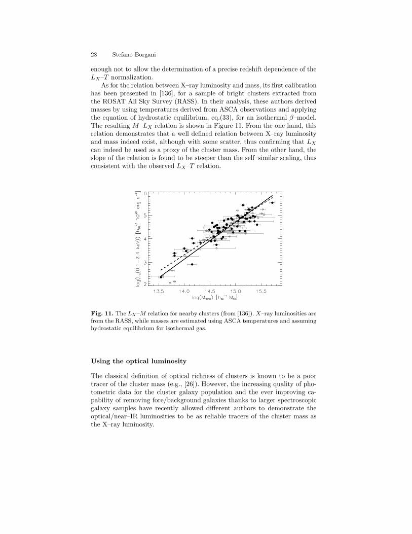
Two examples of recent calibrations between optical/near–IR luminosityand mass are shown in Figure 12. In the left panel we report the result pre-sented in [100], based on K–band luminosites from the 2MASS and massesobtained by applying the M–T relation by [62]. Although the data pointsare rather scattered, they define a clear correlation. Quite interestingly, thebest–fitting relation has a slope shallower than unity, thus indicating the K–band mass-to-light ratio is a (slightly) increasing function of the cluster mass.This result is in line with previous results using optical luminosities (e.g., [72])who found an increasing M/L when passing from galaxy groups to clusters ofincreasing richness.
0.01 0.1 1 10 100
0.01
0.1
1
10
100
Fig. 12. The relation between cluster masses and optical/near-IR luminosities. Leftpanel: M500–L500 relation from [100], using K–band data from the 2MASS surveyand masses from X–ray data. The solid line is the best–fit power law, while thedashed line marks the unity slope. Right panel: the same relation, but in the iSloanband. Open and filled points corresponds to mass estimates based on the SDSSspectroscopic data and on the M–TX relation, respectively.
Popesso et al. [130] analysed SDSS data for a set of clusters which havebeen identified in the RASS. Their mass estimates come from both X–raytemperature [136] and from the velocity dispersions as estimated from theSDSS spectroscopic data. The results of their analysis for the i band are shownin the right panel of Fig. 12. Again, the optical luminosity correlates quitetightly with the cluster mass, with an intrinsic scatter which is comparableto, or even smaller than that of the correlation between X–ray luminosity andmass.
These results highlight how cluster samples with precisely measured opticalluminosities can in principle be usefully employed to constrain cosmologicalparameters. However, while X-ray luminosity provides at the same time a
30 Stefano Borgani
tracer of cluster mass and a criterion to precisely determine the sample selec-tion function, the latter quantity can be extracted from an optically selectedsample only in a rather indirect way.
6 Constraints on cosmological parameters
In this section we will review critically results on cosmological constraintsderived from different ways of tracing the cosmological mass function of galaxyclusters.
6.1 The distribution of velocity dispersions
A first determination of the mass function from velocity dispersions, σv, ofmember galaxies has been attempted in [17]. Girardi et al. [69] used a muchlarger sample of nearby clusters with measured velocity dispersions to comparethe resulting mass function with predictions from cosmological models. Theresulting relation between σ8 and Ωm was such that σ8 ≃ 1 for a fiducial valueof the density parameter Ωm = 0.3. More recently, data for nearby clusters,identified in the SDSS, have been used to calibrate a relation between richnessand velocity dispersion [10]. They compared the resulting σv–distribution tothe prediction of cosmological models and found a significantly lower normal-ization of the power spectrum, σ8 ≃ 0.7 for Ωm = 0.3. Such differences fromdifferent analyses highlight the presence of systematic uncertainties in therelation between mass and observables (i.e., velocity dispersion and richness).
The application of this method to distant clusters has been applied so faronly to the CNOC sample [34], which comprises 17 clusters selected from theEMSS out to z ≃ 0.6. Still to date, this is the only sample of distant clusters,with calibrated selection function, for which velocity dispersions have beenreliably measured. Bahcall et al. [11] pointed out that the resulting evolutionof the mass function is consistent with a low–density Universe. Borgani etal. [24] reanalysed this same sample and emphasised that the uncertainties inthe local normalization of the mass function are large enough to make anyconstraints on Ωm not significant.
6.2 The temperature function
The X-ray Temperature Function (XTF) is defined as the number density ofclusters with given temperature, n(T ). As long as a one-to-one relation existbetween temperature and mass, the XTF can be related to the mass function,n(M), by the relation
n(T ) = n[M(T )]dM
dT. (45)
In this equation, the ratio dM/dT is provided by the relation between ICMtemperature and cluster mass.
Cosmology with clusters of galaxies 31
Measurements of cluster temperatures for flux-limited samples of nearbyclusters were first presented in [83]. These results have been subsequentlyrefined and extended to larger samples with the advent of ROSAT, Beppo–SAX and, especially, ASCA. XTFs have been computed for both nearby (e.g.,[106, 128, 127, 88]) and distant (e.g., [55, 50, 81, 82]) clusters, and used toconstrain cosmological models. The starting point in the computation of theXTF is inevitably a flux-limited sample for which the searching volume ofeach cluster can be computed. Then the LX − TX relation and its scatter isused to derive a temperature limit from the sample flux limit.
Once the XTF is measured from observations, eq.(45) is used to inferthe mass function and, therefore, to constrain cosmological models. A slightlydifferent but conceptually identical approach, has been followed in [136], wheremasses for a flux–limited sample of nearby bright RASS clusters have beencomputed by applying the assumption of hydrostatic equilibrium, therebyexpressing their results directly in terms of mass function, rather than ofXTF.
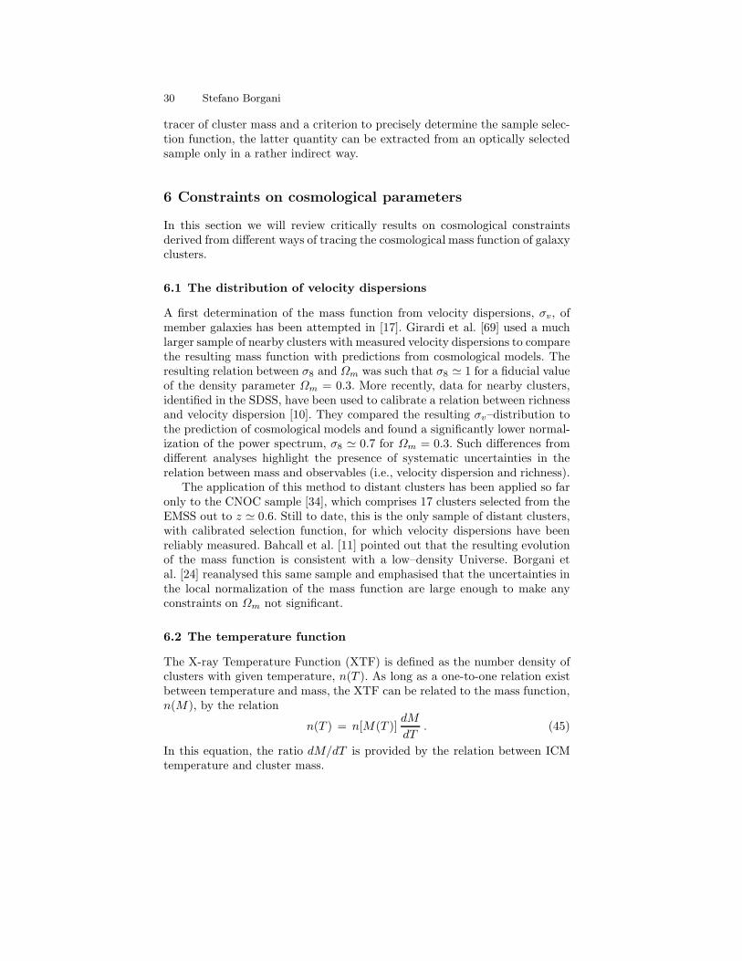
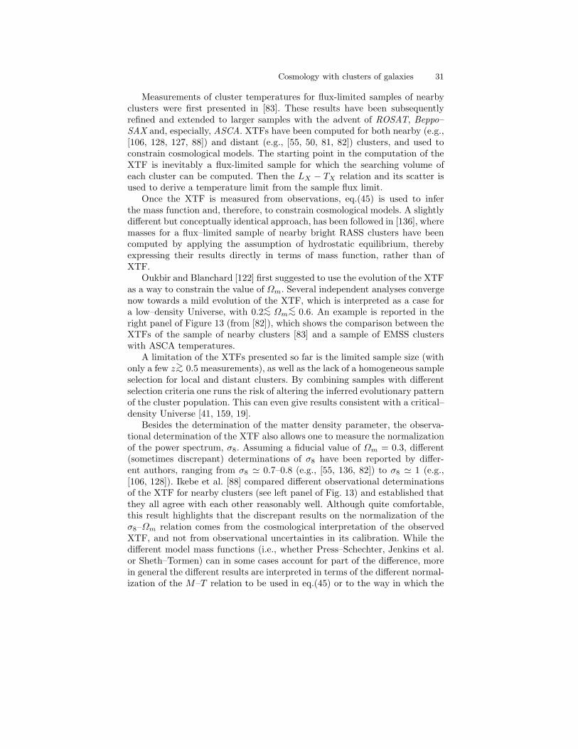
Oukbir and Blanchard [122] first suggested to use the evolution of the XTFas a way to constrain the value of Ωm. Several independent analyses convergenow towards a mild evolution of the XTF, which is interpreted as a case fora low–density Universe, with 0.2∼< Ωm∼< 0.6. An example is reported in theright panel of Figure 13 (from [82]), which shows the comparison between theXTFs of the sample of nearby clusters [83] and a sample of EMSS clusterswith ASCA temperatures.
A limitation of the XTFs presented so far is the limited sample size (withonly a few z∼> 0.5 measurements), as well as the lack of a homogeneous sampleselection for local and distant clusters. By combining samples with differentselection criteria one runs the risk of altering the inferred evolutionary patternof the cluster population. This can even give results consistent with a critical–density Universe [41, 159, 19].
Besides the determination of the matter density parameter, the observa-tional determination of the XTF also allows one to measure the normalizationof the power spectrum, σ8. Assuming a fiducial value of Ωm = 0.3, different(sometimes discrepant) determinations of σ8 have been reported by differ-ent authors, ranging from σ8 ≃ 0.7–0.8 (e.g., [55, 136, 82]) to σ8 ≃ 1 (e.g.,[106, 128]). Ikebe et al. [88] compared different observational determinationsof the XTF for nearby clusters (see left panel of Fig. 13) and established thatthey all agree with each other reasonably well. Although quite comfortable,this result highlights that the discrepant results on the normalization of theσ8–Ωm relation comes from the cosmological interpretation of the observedXTF, and not from observational uncertainties in its calibration. While thedifferent model mass functions (i.e., whether Press–Schechter, Jenkins et al.or Sheth–Tormen) can in some cases account for part of the difference, morein general the different results are interpreted in terms of the different normal-ization of the M–T relation to be used in eq.(45) or to the way in which the
32 Stefano Borgani
Fig. 13. Left panel: a comparison between the XTF for nearby clusters from [88](shaded area), [106] (solid line)and [81] (dotted line). Right panel: the evolution ofthe XTF from [82]. Open and filled circles are for the local and the distant clustersample, respectively.
intrinsic scatter and the statistical uncertainties in this relation are includedin the analysis. We shall critically discuss these issues in Section 6.5 below.
Substantially improved observational determinations of the XTF, and cor-respondingly tighter cosmological constraints, are expected to emerge with theaccumulations of data on the ICM temperature from the Chandra and XMM–Newton satellites. Thanks to the much improved sensitivity of these X–raytelescopes with respect to ASCA, temperature gradients can be measured forfairly large sets of nearby and medium–distant (z∼< 0.4) clusters, thus allow-ing more precise determinations of cluster masses. At the same time, reliablemeasurements of global temperatures are now emerging for clusters out to thehighest redshifts where they have been secured (e.g., [140]). At the time ofwriting, several years after the advent of the new generation of X–ray tele-scopes, no determinations of the XTF from Chandra and XMM–Newton datahave been presented, a situation that is expected to change quite soon.
6.3 The luminosity function
Another method to trace the evolution of the cluster number density is basedon the X–ray luminosity function (XLF), φ(LX), which is defined as the num-ber density of galaxy clusters having a given X–ray luminosity. Similarly toeq.(45), the XLF can be related to the cosmological mass function of collapsedhalos as
φ(LX) = n[M(LX)]dM
dLX, (46)
Cosmology with clusters of galaxies 33
whereM(LX) provides the relation between the observable LX and the clustermass. The above relation needs to be suitably modified in case an intrinsicscatter exists in the relation between mass and temperature (see Section 6.5,here below).
A useful observational quantity, that is related to the XLF, is given bythe flux number–counts, n(S), which is defined as the number of clusters persteradian, having measured flux S:
n(S) =
(
c
H0
)3 ∫ ∞
0
dzr2(z)
E(z)n[M(S, z); z]
dM
dS(47)
(e.g., [94]) where r(z) is the radial coordinate appearing in the Friedmann–Robertson–Walker metric:
r(z)=
∫ z
0
dz E−1(z) ; ΩΛ = 1−Ωm
r(z)=2[
Ωmz + (2 −Ωm) (1−√1 +Ωmz)
]
Ω2m(1 + z)
; ΩΛ = 0 . (48)
The flux S is related to the luminosity according to
S =LX
4πd2L(z), (49)
where dL(z) = r(z)(1 + z) is the luminosity distance at redshift z.This quantity can be measured for a flux–limited samples without having
information on cluster redshift and provides useful cosmological information inthe absence of any spectroscopic optical follow–up. A comparison between dif-ferent observational determinations of the flux number counts for both nearbyand distant cluster samples (e.g., [138]) show indeed a quite good agreement.
Another quantity, which has been used to derive cosmological constraintsfrom flux–limited surveys, is the redshift distribution, n(z), which is definedas the number of clusters found in a survey at a given redshift z:
n(z) =
(
c
H0
)3r2(z)
E(z)
∫ ∞
Slim
dS fsky(S)n[M(S, z); z]dM
dS. (50)
In the above expression Slim is the limiting completeness flux of the survey,while fsky(S) is the effective flux–dependent sky–coverage appropriate for theconsidered survey. Convolving the mass function with the sky coverage insidethe integral in the above equation is essential to properly account for the dif-ferent effective area covered at different fluxes, an aspect which is apparentlyoverlooked in some analyses (e.g., [158]).
In general, the advantage of using X-ray luminosity as a tracer of themass is that LX is measured for a much larger number of clusters in sampleswith well-defined selection properties. As discussed in Section 4.2, the most
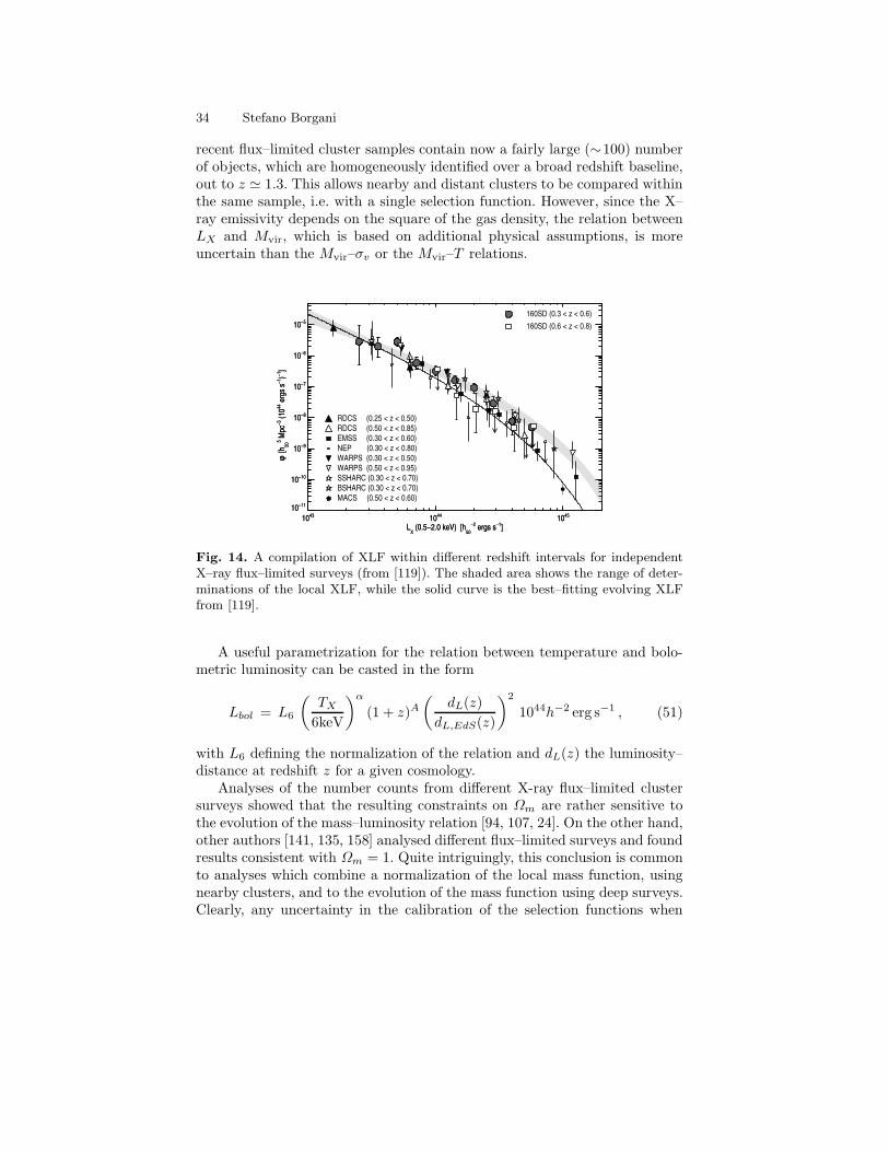
34 Stefano Borgani
recent flux–limited cluster samples contain now a fairly large (∼100) numberof objects, which are homogeneously identified over a broad redshift baseline,out to z ≃ 1.3. This allows nearby and distant clusters to be compared withinthe same sample, i.e. with a single selection function. However, since the X–ray emissivity depends on the square of the gas density, the relation betweenLX and Mvir, which is based on additional physical assumptions, is moreuncertain than the Mvir–σv or the Mvir–T relations.
1043 1044 1045
LX (0.5−2.0 keV) [h
50
−2 ergs s−1]
10−11
10−10
10−9
10−8
10−7
10−6
10−5
φ [h
50
5 Mpc
−3 (
1044
erg
s s−1
)−1]
160SD (0.3 < z < 0.6)
160SD (0.6 < z < 0.8)
1043 1044 1045
LX (0.5−2.0 keV) [h
50
−2 ergs s−1]
10−11
10−10
10−9
10−8
10−7
10−6
10−5
φ [h
50
5 Mpc
−3 (
1044
erg
s s−1
)−1]
RDCS (0.25 < z < 0.50)
RDCS (0.50 < z < 0.85)
EMSS (0.30 < z < 0.60)
NEP (0.30 < z < 0.80)
WARPS (0.30 < z < 0.50)
WARPS (0.50 < z < 0.95)
SSHARC (0.30 < z < 0.70)
BSHARC (0.30 < z < 0.70)
MACS (0.50 < z < 0.60)
Fig. 14. A compilation of XLF within different redshift intervals for independentX–ray flux–limited surveys (from [119]). The shaded area shows the range of deter-minations of the local XLF, while the solid curve is the best–fitting evolving XLFfrom [119].
A useful parametrization for the relation between temperature and bolo-metric luminosity can be casted in the form
Lbol = L6
(
TX
6keV
)α
(1 + z)A(
dL(z)
dL,EdS(z)
)2
1044h−2 erg s−1 , (51)
with L6 defining the normalization of the relation and dL(z) the luminosity–distance at redshift z for a given cosmology.
Analyses of the number counts from different X-ray flux–limited clustersurveys showed that the resulting constraints on Ωm are rather sensitive tothe evolution of the mass–luminosity relation [94, 107, 24]. On the other hand,other authors [141, 135, 158] analysed different flux–limited surveys and foundresults consistent with Ωm = 1. Quite intriguingly, this conclusion is commonto analyses which combine a normalization of the local mass function, usingnearby clusters, and to the evolution of the mass function using deep surveys.Clearly, any uncertainty in the calibration of the selection functions when
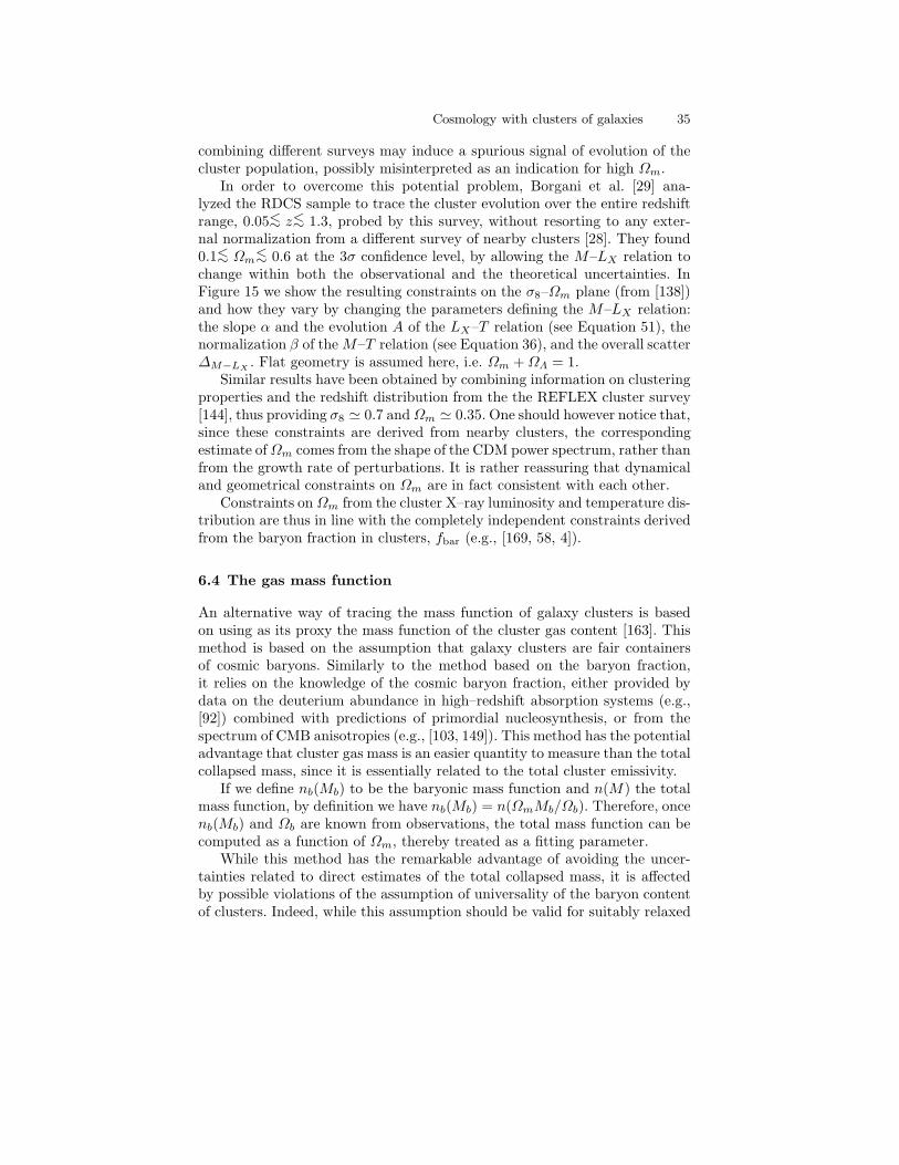
Cosmology with clusters of galaxies 35
combining different surveys may induce a spurious signal of evolution of thecluster population, possibly misinterpreted as an indication for high Ωm.
In order to overcome this potential problem, Borgani et al. [29] ana-lyzed the RDCS sample to trace the cluster evolution over the entire redshiftrange, 0.05∼< z∼< 1.3, probed by this survey, without resorting to any exter-nal normalization from a different survey of nearby clusters [28]. They found0.1∼< Ωm∼< 0.6 at the 3σ confidence level, by allowing the M–LX relation tochange within both the observational and the theoretical uncertainties. InFigure 15 we show the resulting constraints on the σ8–Ωm plane (from [138])and how they vary by changing the parameters defining the M–LX relation:the slope α and the evolution A of the LX–T relation (see Equation 51), thenormalization β of the M–T relation (see Equation 36), and the overall scatter∆M−LX
. Flat geometry is assumed here, i.e. Ωm +ΩΛ = 1.Similar results have been obtained by combining information on clustering
properties and the redshift distribution from the the REFLEX cluster survey[144], thus providing σ8 ≃ 0.7 andΩm ≃ 0.35. One should however notice that,since these constraints are derived from nearby clusters, the correspondingestimate ofΩm comes from the shape of the CDM power spectrum, rather thanfrom the growth rate of perturbations. It is rather reassuring that dynamicaland geometrical constraints on Ωm are in fact consistent with each other.
Constraints on Ωm from the cluster X–ray luminosity and temperature dis-tribution are thus in line with the completely independent constraints derivedfrom the baryon fraction in clusters, fbar (e.g., [169, 58, 4]).
6.4 The gas mass function
An alternative way of tracing the mass function of galaxy clusters is basedon using as its proxy the mass function of the cluster gas content [163]. Thismethod is based on the assumption that galaxy clusters are fair containersof cosmic baryons. Similarly to the method based on the baryon fraction,it relies on the knowledge of the cosmic baryon fraction, either provided bydata on the deuterium abundance in high–redshift absorption systems (e.g.,[92]) combined with predictions of primordial nucleosynthesis, or from thespectrum of CMB anisotropies (e.g., [103, 149]). This method has the potentialadvantage that cluster gas mass is an easier quantity to measure than the totalcollapsed mass, since it is essentially related to the total cluster emissivity.
If we define nb(Mb) to be the baryonic mass function and n(M) the totalmass function, by definition we have nb(Mb) = n(ΩmMb/Ωb). Therefore, oncenb(Mb) and Ωb are known from observations, the total mass function can becomputed as a function of Ωm, thereby treated as a fitting parameter.
While this method has the remarkable advantage of avoiding the uncer-tainties related to direct estimates of the total collapsed mass, it is affectedby possible violations of the assumption of universality of the baryon contentof clusters. Indeed, while this assumption should be valid for suitably relaxed
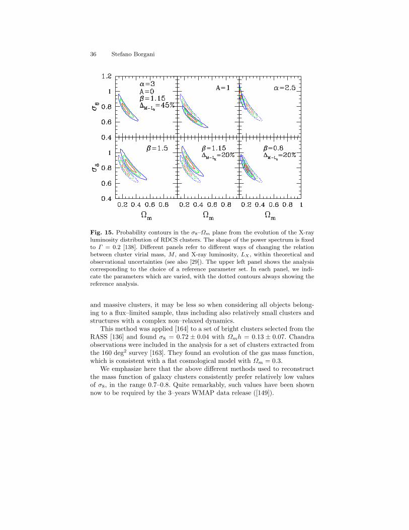
36 Stefano Borgani
Fig. 15. Probability contours in the σ8–Ωm plane from the evolution of the X-rayluminosity distribution of RDCS clusters. The shape of the power spectrum is fixedto Γ = 0.2 [138]. Different panels refer to different ways of changing the relationbetween cluster virial mass, M , and X-ray luminosity, LX , within theoretical andobservational uncertainties (see also [29]). The upper left panel shows the analysiscorresponding to the choice of a reference parameter set. In each panel, we indi-cate the parameters which are varied, with the dotted contours always showing thereference analysis.
and massive clusters, it may be less so when considering all objects belong-ing to a flux–limited sample, thus including also relatively small clusters andstructures with a complex non–relaxed dynamics.
This method was applied [164] to a set of bright clusters selected from theRASS [136] and found σ8 = 0.72 ± 0.04 with Ωmh = 0.13 ± 0.07. Chandraobservations were included in the analysis for a set of clusters extracted fromthe 160 deg2 survey [163]. They found an evolution of the gas mass function,which is consistent with a flat cosmological model with Ωm = 0.3.
We emphasize here that the above different methods used to reconstructthe mass function of galaxy clusters consistently prefer relatively low valuesof σ8, in the range 0.7–0.8. Quite remarkably, such values have been shownnow to be required by the 3–years WMAP data release ([149]).
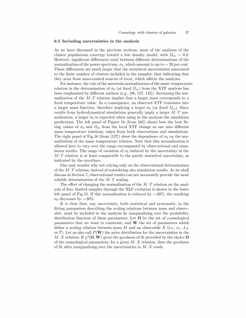
Cosmology with clusters of galaxies 37
6.5 Including uncertainties in the analysis
As we have discussed in the previous sections, most of the analyses of thecluster populations converge toward a low–density model, with Ωm ∼ 0.3.However, significant differences exist between different determinations of thenormalization of the power spectrum, σ8, which amount to up to ∼ 20 per cent.These differences are much larger that the statistical uncertainties associatedto the finite number of clusters included in the samples, thus indicating thatthey arise from unaccounted sources of error, which affects the analyses.
For instance, the role of the uncertain normalization of the mass–temperaturerelation in the determination of σ8 (at fixed Ωm) from the XTF analysis hasbeen emphasized by different authors (e.g., [88, 127, 145]). Increasing the nor-malization of the M–T relation implies that a larger mass corresponds to afixed temperature value. As a consequence, an observed XTF translates intoa larger mass function, therefore implying a larger σ8 (at fixed Ωm). Sinceresults from hydrodynamical simulations generally imply a larger M–T nor-malization, a larger σ8 is expected when using in the analysis the simulationpredictions. The left panel of Figure 16 (from [88]) shows how the best fit-ting values of σ8 and Ωm from the local XTF change as one uses differentmass–temperature relations, taken from both observations and simulations.The right panel of Fig.16 (from [127]) show the dependence of σ8 on the nor-malization of the mass–temperature relation. Note that this normalization isallowed here to vary over the range encompassed by observational and simu-lation results. The range of variation of σ8 induced by the uncertainty in theM–T relation is at least comparable to the purely statistical uncertainty, asindicated by the errorbars.
One may wonder why not relying only on the observational determinationof the M–T relation, instead of considering also simulation results. As we shalldiscuss in Section 7, observational results can not necessarily provide the mostreliable determination of the M–T scaling.
The effect of changing the normalization of the M–T relation on the anal-ysis of flux–limited samples through the XLF evolution is shown in the lowerleft panel of Fig.15. If this normalization is reduced by ∼ 30%, the resultingσ8 decreases by ∼20%.
It is clear that, any uncertainty, both statistical and systematic, in thefitting parameters describing the scaling relations between mass and observ-able, must be included in the analysis by marginalizing over the probabilitydistribution function of these parameters. Let Ω be the set of cosmologicalparameters that we want to constrain, and W the set of parameters whichdefine a scaling relation between mass M and an observable X (i.e., σv, LX
or T ). Let us also call P (W) the prior distribution for the uncertainties in theM–X relation. If χ2(Ω,W) gives the goodness of fit provided by the choice Ωof the cosmological parameters, for a given M–X relation, then the goodnessof fit after marginalizing over the uncertainties in M–X reads
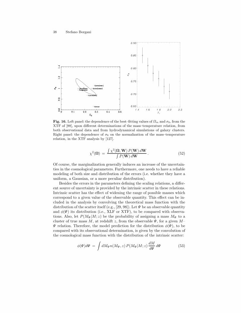
38 Stefano Borgani
Fig. 16. Left panel: the dependence of the best–fitting values of Ωm and σ8, from theXTF of [88], upon different determinations of the mass–temperature relation, fromboth observational data and from hydrodynamical simulations of galaxy clusters.Right panel: the dependence of σ8 on the normalization of the mass–temperaturerelation, in the XTF analysis by [127].
χ2(Ω) =
∫
χ2(Ω,W)P (W) dW∫
P (W) dW. (52)
Of course, the marginalization generally induces an increase of the uncertain-ties in the cosmological parameters. Furthermore, one needs to have a reliablemodeling of both size and distribution of the errors (i.e. whether they have auniform, a Gaussian, or a more peculiar distribution).
Besides the errors in the parameters defining the scaling relations, a differ-ent source of uncertainty is provided by the intrinsic scatter in these relations.Intrinsic scatter has the effect of widening the range of possible masses whichcorrespond to a given value of the observable quantity. This effect can be in-cluded in the analysis by convolving the theoretical mass function with thedistribution of the scatter itself (e.g., [29, 98]). Let Ψ be an observable quantityand φ(Ψ) its distribution (i.e., XLF or XTF), to be compared with observa-tions. Also, let P (MΨ |M ; z) be the probability of assigning a mass MΨ to acluster of true mass M , at redshift z, from the observable Ψ , for a given M–Ψ relation. Therefore, the model prediction for the distribution φ(Ψ), to becompared with its observational determination, is given by the convolution ofthe cosmological mass function with the distribution of the intrinsic scatter:
φ(Ψ)dΨ =
∫
dMΨn(MΨ , z)P (MΨ |M ; z)dM
dΨdΨ (53)
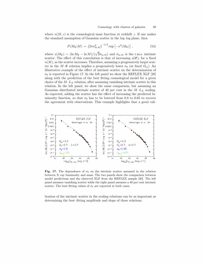
Cosmology with clusters of galaxies 39
where n(M, z) is the cosmological mass function at redshift z. If one makesthe standard assumption of Gaussian scatter in the log–log plane, then
P (MΨ |M) =(
2πσ2lnM
)−1/2exp
[
−x2(MΨ )]
, (54)
where x(MΨ ) = (lnMΨ − lnM)/(√2σlnM ) and σlnM is the r.m.s. intrinsic
scatter. The effect of this convolution is that of increasing φ(Ψ), for a fixedn(M), as the scatter increases. Therefore, assuming a progressively larger scat-ter in the M–Ψ relation implies a progressively lower σ8 (at fixed Ωm). Anillustrative example of the effect of intrinsic scatter on the determination ofσ8 is reported in Figure 17. In the left panel we show the REFLEX XLF [20]along with the prediction of the best fitting cosmological model for a givenchoice of the M–LX relation, after assuming vanishing intrinsic scatter in thisrelation. In the left panel, we show the same comparison, but assuming anGaussian–distributed intrinsic scatter of 40 per cent in the M–LX scaling.As expected, adding the scatter has the effect of increasing the predicted lu-minosity function, so that σ8 has to be lowered from 0.8 to 0.65 to recoverthe agreement with observations. This example highlights that a good cali-
Fig. 17. The dependence of σ8 on the intrinsic scatter assumed in the relationbetween X–ray luminosity and mass. The two panels show the comparison betweenmodel predictions and the observed XLF from the REFLEX sample [20]. The leftpanel assumes vanishing scatter while the right panel assumes a 40 per cent intrinsicscatter. The best fitting values of σ8 are reported in both cases.
bration of the intrinsic scatter in the scaling relations can be as important asdetermining the best–fitting amplitude and slope of these relations.
40 Stefano Borgani
7 The future
A new era for cosmology with galaxy clusters is now starting. High sensitivitysurveys for blind SZ identification over fairly large contiguous area, ∼ 100deg2, have have already started or are planned in the coming years (see thelectures by M. Birkinshaw in this volume). Also, the Planck satellite willsurvey the whole sky, although at a much lower sensitivity, and provide alarge set of clusters identified through the SZ effect. These surveys promiseto identify several thousands clusters, with a fair number of objects expectedto be found at z > 1. In the optical/near-IR bands, imaging with dedicatedtelescopes with large field of view will also allow to secure a large number ofdistant clusters. At the same time, X–ray observations over contiguous area(e.g., [170] and “serendipitous” searches from XMM–Newton (e.g., [118]) andChandra (e.g., [30]) archives will ultimately cover several hundreds deg2 downto flux limits fainter than those reached by the deepest ROSAT pointings.Preliminary results suggest that identification of z > 1 clusters may eventuallybecome routine [118]. Ultimately, they will lead to the identification of severalthousands clusters.
Optimized optics for wide–field X–ray imaging have been originally de-scribed in a far-reaching paper by Burrows et al. [33] and proposed for thefirst time to be implemented in a dedicated satellite mission in the mid 90’s.There is no doubt that this would be the right time to plan a dedicatedwide–field X–ray telescope, which should survey the sky over an area of sev-eral thousands deg2, with a relatively good, XMM–like or better, point spreadfunction and a low background. This instrument would be invaluable for stud-ies of galaxy clusters, thanks to its ability of both identifying extended sourceswith low surface brightness. Several missions with a similar profile have beenproposed, although none has been approved so far. Still, the community work-ing on galaxy clusters is regularly proposing this idea of satellite to differentSpace Agencies (e.g., [79]).
The samples of galaxy clusters obtainable from large–area SZ and X–raysurveys contain in principle so much information to allow one to constrain notonly Ωm and σ8, but also the Dark Energy (DE) content of the Universe (see,e.g., [153, 142] for introductory reviews on Dark Energy). The equation ofstate of DE is written in the form p = wρ, where p and ρ are the pressure anddensity terms, respectively. The parameter w must take values in the range−1/3 > w ≥ −1 for the DE to provide an accelerated cosmic expansion.Constraining the value of w and its redshift evolution is currently consideredone of the most ambitious targets of modern cosmology. Ones hope is to unveilthe nature of the energy term which dominates the overall dynamics of theUniverse at the present time.
As we have mentioned, the limited statistics prevents current cluster sur-veys to place significant constraints on ΩΛ. Although this limitation will beovercome with future cluster surveys, the question remains as to whether thesystematic effects, discussed in Section 6.5, can be sufficiently understood.
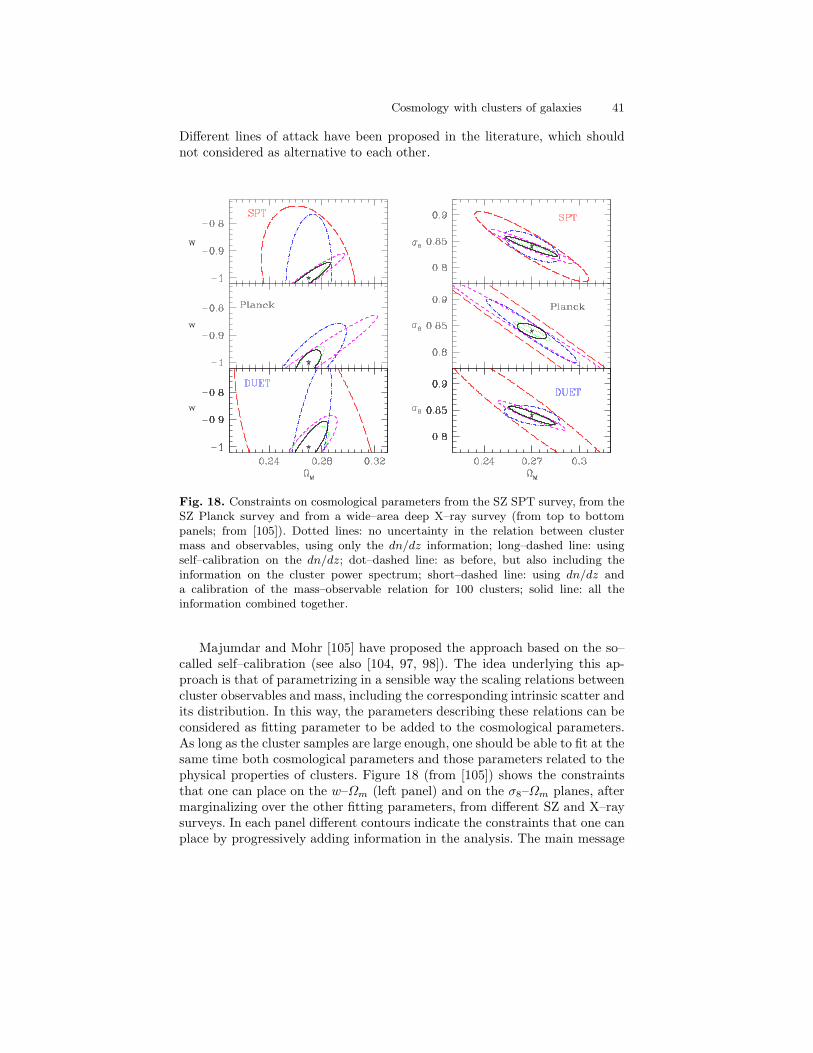
Cosmology with clusters of galaxies 41
Different lines of attack have been proposed in the literature, which shouldnot considered as alternative to each other.
Fig. 18. Constraints on cosmological parameters from the SZ SPT survey, from theSZ Planck survey and from a wide–area deep X–ray survey (from top to bottompanels; from [105]). Dotted lines: no uncertainty in the relation between clustermass and observables, using only the dn/dz information; long–dashed line: usingself–calibration on the dn/dz; dot–dashed line: as before, but also including theinformation on the cluster power spectrum; short–dashed line: using dn/dz anda calibration of the mass–observable relation for 100 clusters; solid line: all theinformation combined together.
Majumdar and Mohr [105] have proposed the approach based on the so–called self–calibration (see also [104, 97, 98]). The idea underlying this ap-proach is that of parametrizing in a sensible way the scaling relations betweencluster observables and mass, including the corresponding intrinsic scatter andits distribution. In this way, the parameters describing these relations can beconsidered as fitting parameter to be added to the cosmological parameters.As long as the cluster samples are large enough, one should be able to fit at thesame time both cosmological parameters and those parameters related to thephysical properties of clusters. Figure 18 (from [105]) shows the constraintsthat one can place on the w–Ωm (left panel) and on the σ8–Ωm planes, aftermarginalizing over the other fitting parameters, from different SZ and X–raysurveys. In each panel different contours indicate the constraints that one canplace by progressively adding information in the analysis. The main message
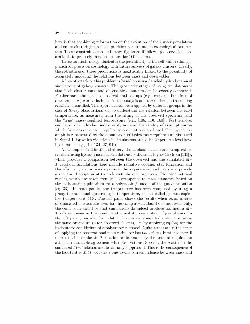
42 Stefano Borgani
here is that combining information on the evolution of the cluster populationand on its clustering can place precision constraints on cosmological parame-ters. These constraints can be further tightened if follow up observations areavailable to precisely measure masses for 100 clusters.
These forecasts nicely illustrates the potentiality of the self–calibration ap-proach for precision cosmology with future surveys of galaxy clusters. Clearly,the robustness of these predictions is inextricably linked to the possibility ofaccurately modeling the relations between mass and observables.
A line of attack to this problem is based on using detailed hydrodynamicalsimulations of galaxy clusters. The great advantages of using simulations isthat both cluster mass and observable quantities can be exactly computed.Furthermore, the effect of observational set–ups (e.g., response functions ofdetectors, etc.) can be included in the analysis and their effect on the scalingrelations quantified. This approach has been applied by different groups in thecase of X–ray observations [64] to understand the relation between the ICMtemperature, as measured from the fitting of the observed spectrum, andthe “true” mass–weighted temperature (e.g., [108, 110, 160]). Furthermore,simulations can also be used to verify in detail the validity of assumptions onwhich the mass estimators, applied to observations, are based. The typical ex-ample is represented by the assumption of hydrostatic equilibrium, discussedin Sect.5.1, for which violations in simulations at the 10–20 per cent level havebeen found (e.g., [12, 134, 27, 91]).
An example of calibration of observational biases in the mass–temperaturerelation, using hydrodynamical simulations, is shown in Figure 19 (from [133]),which provides a comparison between the observed and the simulated M–T relation. Simulations here include radiative cooling, star formation andthe effect of galactic winds powered by supernovae, and, as such, providea realistic description of the relevant physical processes. The observationalresults, which are taken from [62], corresponds to mass estimates based onthe hydrostatic equilibrium for a polytropic β–model of the gas distribution[eq.(33)]. In both panels, the temperature has been computed by using aproxy to the actual spectroscopic temperature, the so–called spectroscopic–like temperature [110]. The left panel shows the results when exact massesof simulated clusters are used for the comparison. Based on this result only,the conclusion would be that simulations do indeed produce too high a M–T relation, even in the presence of a realistic description of gas physics. Inthe left panel, masses of simulated clusters are computed instead by usingthe same procedure as for observed clusters, i.e. by applying eq.(34) for thehydrostatic equilibrium of a polytropic β–model. Quite remarkably, the effectof applying the observational mass estimator has two effects. First, the overallnormalization of the M–T relation is decreased by the amount required toattain a reasonable agreement with observations. Second, the scatter in thesimulatedM–T relation is substantially suppressed. This is the consequence ofthe fact that eq.(34) provides a one-to-one correspondence between mass and
Cosmology with clusters of galaxies 43
Fig. 19. The mass–temperature relation at ρ/ρcr = 500, in simulations (filled circlesand triangles) and for the observational data (squares with errorbars, [62]). The leftpanel is for the true masses of simulated clusters; the right panel is for masses ofsimulated clusters estimated by adopting the same procedure applied by Finoguenovet al. to observational data (from [133]).
temperature, while only the cluster-by-cluster variations of β and γ accountfor the intrinsic diversity of the cluster thermal structure.
This example illustrates how simulations can be usefully employed asguidelines to study possible biases on observational mass estimates. However,it is worth reminding that the reliability of simulation results depends onour capability to correctly provide a numerical description of all the relevantphysical process. In this sense, understanding in detail the (astro)physics ofclusters is mandatory in order to calibrate them as tools in the era of precisioncosmology.
As a concluding remark, we emphasize once more that a number of inde-pendent analysesof the cluster mass function, which have been realized so far,favor a relatively low normalization of the power spectrum, with σ8 ≃ 0.7–0.8for Ωm ≃ 0.3, thus in agreement with the most recent WMAP results ([149]).This agreement must be considered as a success for cluster cosmology anda strong encourgement for future applications to large cluster surveys of thenext generation.
Acknowledgments. I would like to thank the organizers of the GH2005School, David Hughes, Omar Lopez–Cruz and Manolis Plionis for having pro-vided an enjoyable and stimulating environment. I also warmly thank ManolisPlionis and Piero Rosati for a careful reading of the manuscript and usefulsuggestions to improve it.
44 Stefano Borgani
References
1. Abell G. O., 1958, ApJS, 3, 2112. Abell G. O., Corwin H. G., Olowin R. P., 1989, ApJS, 70, 13. Allen S. W., Fabian A. C., 1998, MNRAS, 297, L574. Allen S. W., Schmidt R. W., Ebeling H., Fabian A. C., van Speybroeck L., 2004,
MNRAS, 353, 4575. Allen S. W., Schmidt R. W., Fabian A. C., 2001, MNRAS, 328, L376. Allen S. W., Schmidt R. W., Fabian A. C., 2002, MNRAS, 334, L117. Arnaud M., Evrard A. E., 1999, MNRAS, 305, 6318. Arnaud M., Pointecouteau E., Pratt G. W., 2005, A&A, 441, 8939. Bahcall N. A., Cen R., Dav e R., Ostriker J. P., Yu Q., 2000, ApJ, 541, 1
10. Bahcall N. A., Dong F., Bode P., Kim R., Annis J., McKay T. A., Hansen S.,Schroeder J., Gunn J., Ostriker J. P., Postman M., Nichol R. C., Miller C., GotoT., Brinkmann J., Knapp G. R., Lamb D. O., Schneider D. P., Vogeley M. S.,York D. G., 2003, ApJ, 585, 182
11. Bahcall N. A., Fan X., Cen R., 1997, ApJ, 485, L53+12. Bartelmann M., Steinmetz M., 1996, MNRAS, 283, 43113. Basilakos, S., Plionis, M., Georgakakis, A., Georgantopoulos, I., Gaga, T.,
Kolokotronis, V., Stewart, G., 2004, MNRAS, 351, 98914. Binney J., Tremaine S., 1987, Galactic dynamics . Princeton, NJ, Princeton
University Press, 1987, 747 p.15. Birkinshaw M., 1999, Phys. Rep., 310, 9716. Biviano A., Girardi M., 2003, ApJ, 585, 20517. Biviano A., Girardi M., Giuricin G., Mardirossian F., Mezzetti M., 1993, ApJ,
411, L1318. Biviano A., Murante G., Borgani S., Diaferio A., Dolag K., Girardi M., 2006,
ArXiv Astrophysics e-prints19. Blanchard A., Sadat R., Bartlett J. G., Le Dour M., 2000, A&A, 362, 80920. B o hringer H., Collins C. A., Guzzo L., Schuecker P., Voges W., Neumann
D. M., Schindler S., Chincarini G., De Grandi S., Cruddace R. G., Edge A. C.,Reiprich T. H., Shaver P., 2002, ApJ, 566, 93
21. B o hringer H., Schuecker P., Guzzo L., Collins C. A., Voges W., CruddaceR. G., Ortiz-Gil A., Chincarini G., De Grandi S., Edge A. C., MacGillivrayH. T., Neumann D. M., Schindler S., Shaver P., 2004, A&A, 425, 367
22. B o hringer H., Voges W., Huchra J. P., McLean B., Giacconi R., Rosati P., BurgR., Mader J., Schuecker P., Simi c D., Komossa S., Reiprich T. H., Retzlaff J.,Tr u mper J., 2000, ApJS, 129, 435
23. Bond J. R., Cole S., Efstathiou G., Kaiser N., 1991, ApJ, 379, 44024. Borgani S., Girardi M., Carlberg R. G., Yee H. K. C., Ellingson E., 1999, ApJ,
527, 56125. Borgani S., Governato F., Wadsley J., Menci N., Tozzi P., Quinn T., Stadel J.,
Lake G., 2002, MNRAS, 336, 40926. Borgani S., Guzzo L., 2001, Nature, 409, 3927. Borgani S., Murante G., Springel V., Diaferio A., Dolag K., Moscardini L.,
Tormen G., Tornatore L., Tozzi P., 2004, MNRAS, 348, 107828. Borgani S., Rosati P., Tozzi P., Norman C., 1999, ApJ, 517, 4029. Borgani S., Rosati P., Tozzi P., Stanford S. A., Eisenhardt P. R., Lidman C.,
Holden B., Della Ceca R., Norman C., Squires G., 2001, ApJ, 561, 13
Cosmology with clusters of galaxies 45
30. Boschin W., 2002, A&A, 396, 39731. Bryan G. L., Norman M. L., 1998, ApJ, 495, 8032. Burke D. J., Collins C. A., Sharples R. M., Romer A. K., Holden B. P., Nichol
R. C., 1997, ApJ, 488, L83+33. Burrows C. J., Burg R., Giacconi R., 1992, ApJ, 392, 76034. Carlberg R. G., Morris S. L., Yee H. K. C., Ellingson E., 1997, ApJ, 479, L19+35. Carlberg R. G., Yee H. K. C., Ellingson E., Abraham R., Gravel P., Morris S.,
Pritchet C. J., 1996, ApJ, 462, 3236. Carlberg R. G., Yee H. K. C., Ellingson E., Morris S. L., Abraham R., Gravel
P., Pritchet C. J., Smecker-Hane T., Hartwick F. D. A., Hesser J. E., HutchingsJ. B., Oke J. B., 1997, ApJ, 476, L7+
37. Carlstrom J. E., Holder G. P., Reese E. D., 2002, ARAA, 40, 64338. Castander F. J., Bower R. G., Ellis R. S., Aragon-Salamanca A., Mason K. O.,
Hasinger G., McMahon R. G., Carrera F. J., Mittaz J. P. D., Perez-Fournon I.,Lehto H. J., 1995, Nature, 377, 39
39. Cavaliere A., Fusco-Femiano R., 1976, A&A, 49, 13740. Cavaliere A., Gursky H., Tucker W., 1971, Nature, 231, 43741. Colafrancesco S., Mazzotta P., Vittorio N., 1997, ApJ, 488, 56642. Coles P., Lucchin F., 2002, Cosmology: The Origin and Evolution of Cosmic
Structure, Second Edition . Cosmology: The Origin and Evolution of CosmicStructure, Second Edition, by Peter Coles, Francesco Lucchin, pp. 512. ISBN0-471-48909-3. Wiley-VCH , July 2002.
43. Couch W. J., Ellis R. S., MacLaren I., Malin D. F., 1991, MNRAS, 249, 60644. Dalcanton J. J., 1996, ApJ, 466, 9245. Dalton G. B., Maddox S. J., Sutherland W. J., Efstathiou G., 1997, MNRAS,
289, 26346. Davis M., Peebles P. J. E., 1983, ApJ, 267, 46547. Diaferio A., Borgani S., Moscardini L., Murante G., Dolag K., Springel V.,
Tormen G., Tornatore L., Tozzi P., 2005, MNRAS, 356, 147748. Donahue, Megan, Scharf, Caleb A., Mack, Jennifer, Lee, Y. Paul, Postman,
Marc, Rosati, Piero, Dickinson, Mark, Voit, G. Mark, Stocke, John T., 2002,ApJ, 569, 689
49. Donahue M., Mack J., Scharf C., Lee P., Postman M., Rosati P., Dickinson M.,Voit G. M., Stocke J. T., 2001, ApJ, 552, L93
50. Donahue M., Voit G. M., 1999, ApJ, 523, L13751. Ebeling H., Edge A. C., Allen S. W., Crawford C. S., Fabian A. C., Huchra
J. P., 2000, MNRAS, 318, 33352. Ebeling H., Edge A. C., Henry J. P., 2001, ApJ, 553, 66853. Eisenstein D. J., Hu W., 1999, ApJ, 511, 554. Eke V. R., Cole S., Frenk C. S., 1996, MNRAS, 282, 26355. Eke V. R., Cole S., Frenk C. S., Patrick Henry J., 1998, MNRAS, 298, 114556. Ettori S., De Grandi S., Molendi S., 2002, A&A, 391, 84157. Ettori S., Tozzi P., Borgani S., Rosati P., 2004, A&A, 417, 1358. Ettori S., Tozzi P., Rosati P., 2003, A&A, 398, 87959. Evrard A. E., MacFarland T. J., Couchman H. M. P., Colberg J. M., Yoshida N.,
White S. D. M., Jenkins A., Frenk C. S., Pearce F. R., Peacock J. A., ThomasP. A., 2002, ApJ, 573, 7
60. Fabian A. C., 1991, MNRAS, 253, 29P61. Felten J. E., Gould R. J., Stein W. A., Woolf N. J., 1966, ApJ, 146, 955
46 Stefano Borgani
62. Finoguenov A., Reiprich T. H., B o hringer H., 2001, A&A, 368, 74963. Frenk C. S., Evrard A. E., White S. D. M., Summers F. J., 1996, ApJ, 472, 46064. Gardini A., Rasia E., Mazzotta P., Tormen G., De Grandi S., Moscardini L.,
2004, MNRAS, 351, 50565. Giacconi R., Branduardi G., Briel U., et al. 1979, ApJ, 230, 54066. Giacconi R., Murray S., Gursky H., Kellogg E., Schreier E., Tananbaum H.,
1972, ApJ, 178, 28167. Gioia I. M., Henry J. P., Maccacaro T., Morris S. L., Stocke J. T., Wolter A.,
1990, ApJ, 356, L3568. Girardi M., Biviano A., Giuricin G., Mardirossian F., Mezzetti M., 1993, ApJ,
404, 3869. Girardi M., Borgani S., Giuricin G., Mardirossian F., Mezzetti M., 1998, ApJ,
506, 4570. Girardi M., Borgani S., Giuricin G., Mardirossian F., Mezzetti M., 2000, ApJ,
530, 6271. Girardi M., Giuricin G., Mardirossian F., Mezzetti M., Boschin W., 1998, ApJ,
505, 7472. Girardi M., Manzato P., Mezzetti M., Giuricin G., Limboz F., 2002, ApJ, 569,
72073. Girardi M., Mezzetti M., 2001, ApJ, 548, 7974. Gladders M. D., Yee H. K. C., 2005, ApJS, 157, 175. Gonzalez A. H., Zaritsky D., Dalcanton J. J., Nelson A., 2001, ApJS, 137, 11776. Governato F., Babul A., Quinn T., Tozzi P., Baugh C. M., Katz N., Lake G.,
1999, MNRAS, 307, 94977. Gross M. A. K., Somerville R. S., Primack J. R., Holtzman J., Klypin A., 1998,
MNRAS, 301, 8178. Gunn J. E., Hoessel J. G., Oke J. B., 1986, ApJ, 306, 3079. Haiman Z., Allen S., Bahcall N., et al. 2005, ArXiv Astrophysics e-prints80. Haiman Z., Mohr J. J., Holder G. P., 2001, ApJ, 553, 54581. Henry J. P., 2000, ApJ, 534, 56582. Henry J. P., 2004, ApJ, 609, 60383. Henry J. P., Arnaud K. A., 1991, ApJ, 372, 41084. Henry J. P., Gioia I. M., Maccacaro T., Morris S. L., Stocke J. T., Wolter A.,
1992, ApJ, 386, 40885. Henry J. P., Gioia I. M., Mullis C. R., Voges W., Briel U. G., B o hringer H.,
Huchra J. P., 2001, ApJ, 553, L10986. Holden B. P., Stanford S. A., Squires G. K., Rosati P., Tozzi P., Eisenhardt P.,
Spinrad H., 2002, AJ, 124, 3387. Hu W., Kravtsov A. V., 2003, ApJ, 584, 70288. Ikebe Y., Reiprich T. H., B o hringer H., Tanaka Y., Kitayama T., 2002, A&A,
383, 77389. Jenkins A., Frenk C., White S., Colberg J., Cole S., Evrard A., Couchman H.,
Yoshida N., 2001, MNRAS, 321, 37290. Kaiser N., 1986, MNRAS, 222, 32391. Kay S. T., Thomas P. A., Jenkins A., Pearce F. R., 2004, MNRAS, 355, 109192. Kirkman D., Tytler D., Suzuki N., O’Meara J. M., Lubin D., 2003, ApJS, 149,
193. Kitayama T., Suto Y., 1996, ApJ, 469, 48094. Kitayama T., Suto Y., 1997, ApJ, 490, 557
Cosmology with clusters of galaxies 47
95. Kotov O., Vikhlinin A., 2005, ApJ, 633, 78196. Lewis A. D., Ellingson E., Morris S. L., Carlberg R. G., 1999, ApJ, 517, 58797. Lima M., Hu W., 2004, Phys. Rev. D, 70, 04350498. Lima M., Hu W., 2005, Phys. Rev. D, 72, 04300699. Limber D. N., Mathews W. G., 1960, ApJ, 132, 286100. Lin Y.-T., Mohr J. J., Stanford S. A., 2003, ApJ, 591, 749101. Lumb D. H., Bartlett J. G., Romer A. K., Blanchard A., Burke D. J., Collins
C. A., Nichol R. C., Giard M., Marty P. B., Nevalainen J., Sadat R., VauclairS. C., 2004, A&A, 420, 853
102. Lumsden S. L., Nichol R. C., Collins C. A., Guzzo L., 1992, MNRAS, 258, 1103. MacTavish C., Ade P. A. R., Bock J. J., et al. 2005, ArXiv Astrophysics e-prints104. Majumdar S., Mohr J. J., 2003, ApJ, 585, 603105. Majumdar S., Mohr J. J., 2004, ApJ, 613, 41106. Markevitch M., 1998, ApJ, 504, 27107. Mathiesen B., Evrard A. E., 1998, MNRAS, 295, 769108. Mathiesen B. F., Evrard A. E., 2001, ApJ, 546, 100109. Maughan B. J., Jones L. R., Ebeling H., Scharf C., 2006, MNRAS, 365, 509110. Mazzotta P., Rasia E., Moscardini L., Tormen G., 2004, MNRAS, 354, 10111. Miller C. J., Nichol R. C., Reichart D., et al. 2005, AJ, 130, 968112. Monaco P., 1998, Fundamentals of Cosmic Physics, 19, 157113. Moretti A., Guzzo L., Campana S., Lazzati D., Panzera M. R., Tagliaferri G.,
Arena S., Braglia F., Dell’Antonio I., Longhetti M., 2004, A&A, 428, 21114. Moscardini L., Matarrese S., Mo H. J., 2001, MNRAS, 327, 422115. Motl P. M., Hallman E. J., Burns J. O., Norman M. L., 2005, ApJ, 623, L63116. Mulchaey J. S., Zabludoff A. I., 1998, ApJ, 496, 73117. Mullis C. R., McNamara B. R., Quintana H., Vikhlinin A., Henry J. P., Gioia
I. M., Hornstrup A., Forman W., Jones C., 2003, ApJ, 594, 154118. Mullis C. R., Rosati P., Lamer G., B o hringer H., Schwope A., Schuecker P.,
Fassbender R., 2005, ApJ, 623, L85119. Mullis C. R., Vikhlinin A., Henry J. P., Forman W., Gioia I. M., Hornstrup
A., Jones C., McNamara B. R., Quintana H., 2004, ApJ, 607, 175120. Nevalainen J., Markevitch M., Forman W., 2000, ApJ, 532, 694121. Osmond J. P. F., Ponman T. J., 2004, MNRAS, 350, 1511122. Oukbir J., Blanchard A., 1992, A&A, 262, L21123. Peacock J. A., 1999, Cosmological Physics . Cosmological Physics, by John
A. Peacock, pp. 704. ISBN 052141072X. Cambridge, UK: Cambridge UniversityPress, January 1999.
124. Peebles P. J. E., 1993, Principles of physical cosmology . Princeton Series inPhysics, Princeton, NJ: Princeton University Press, —c1993
125. Perlman E. S., Horner D. J., Jones L. R., Scharf C. A., Ebeling H., WegnerG., Malkan M., 2002, ApJS, 140, 265
126. Piccinotti G., Mushotzky R. F., Boldt E. A., Holt S. S., Marshall F. E., Ser-lemitsos P. J., Shafer R. A., 1982, ApJ, 253, 485
127. Pierpaoli E., Borgani S., Scott D., White M., 2003, MNRAS, 342, 163128. Pierpaoli E., Scott D., White M., 2001, MNRAS, 325, 77129. Plionis, M., Basilakos, S., Georgantopoulos, I., Georgakakis, A., 2005, ApJ,
622, L17130. Popesso P., Biviano A., B o hringer H., Romaniello M., Voges W., 2005, A&A,
433, 431
48 Stefano Borgani
131. Postman M., Lubin L. M., Gunn J. E., Oke J. B., Hoessel J. G., SchneiderD. P., Christensen J. A., 1996, AJ, 111, 615
132. Press W., Schechter P., 1974, ApJ, 187, 425133. Rasia E., Mazzotta P., Borgani S., Moscardini L., Dolag K., Tormen G., Di-
aferio A., Murante G., 2005, ApJ, 618, L1134. Rasia E., Tormen G., Moscardini L., 2004, MNRAS, 351, 237135. Reichart D. E., Nichol R. C., Castander F. J., Burke D. J., Romer A. K.,
Holden B. P., Collins C. A., Ulmer M. P., 1999, ApJ, 518, 521136. Reiprich T., B o hringer H., 2002, ApJ, 567, 716137. Rines K., Geller M. J., Kurtz M. J., Diaferio A., 2003, AJ, 126, 2152138. Rosati P., Borgani S., Norman C., 2002, ARAA, 40, 539139. Rosati P., della Ceca R., Norman C., Giacconi R., 1998, ApJ, 492, L21+140. Rosati P., Tozzi P., Ettori S., Mainieri V., Demarco R., Stanford S. A., Lidman
C., Nonino M., Borgani S., Della Ceca R., Eisenhardt P., Holden B. P., NormanC., 2004, AJ, 127, 230
141. Sadat R., Blanchard A., Oukbir J., 1998, A&A, 329, 21142. Sahni V., 2005, LNP Vol. 653: The Physics of the Early Universe, 653, 141143. Schuecker P., B o hringer H., Guzzo L., Collins C. A., Neumann D. M.,
Schindler S., Voges W., De Grandi S., Chincarini G., Cruddace R., M u llerV., Reiprich T. H., Retzlaff J., Shaver P., 2001, A&A, 368, 86
144. Schuecker P., Guzzo L., Collins C. A., B o hringer H., 2002, MNRAS, 335, 807145. Seljak U., 2002, MNRAS, 337, 769146. Sheth R., Tormen G., 1999, MNRAS, 308, 119147. Sheth R. K., Tormen G., 2002, MNRAS, 329, 61148. Smith S., 1936, ApJ, 83, 23149. Spergel D. N., Bean R., Dore O., Nolta M. R., Bennett, C. L., Hinshaw G.,
Jarosik N., Komatsu E., Page L., Peiris H. V., Verde L., Barnes C., Halpern M.,Hill R. S., Kogut A., Limon M., Meyer S. S., Odegard N., Tucker G. S., WeilandJ. L., Wollack E., Wright E. L., 2006, ArXiv Astrophysics e-prints
150. Springel V., White S. D. M., Jenkins A., Frenk C. S., Yoshida N., Gao L.,Navarro J., Thacker R., Croton D., Helly J., Peacock J. A., Cole S., Thomas P.,Couchman H., Evrard A., Colberg J., Pearce F., 2005, Nature, 435, 629
151. Stanford S. A., Holden B., Rosati P., Eisenhardt P. R., Stern D., Squires G.,Spinrad H., 2002, AJ, 123, 619
152. Stanford S. A., et al., 2005, ApJ, 634, L129153. Steinhardt P. J., 2003, Royal Society of London Philosophical Transactions
Series A, 361, 2497154. Stoughton C., Lupton R. H., Bernardi M., et al. 2002, AJ, 123, 485155. Sunyaev R. A., Zeldovich Y. B., 1972, Comments on Astrophysics and Space
Physics, 4, 173156. Truemper J., 1993, Science, 260, 1769157. van Haarlem M. P., Frenk C. S., White S. D. M., 1997, MNRAS, 287, 817158. Vauclair S. C., Blanchard A., Sadat R., Bartlett J. G., Bernard J.-P., Boer M.,
Giard M., Lumb D. H., Marty P., Nevalainen J., 2003, A&A, 412, L37159. Viana P. T. P., Liddle A. R., 1999, MNRAS, 303, 535160. Vikhlinin A., 2006, ApJ, 640, 710161. Vikhlinin A., Kravtsov A., Forman W., Jones C., Markevitch M., Murray S. S.,
Van Speybroeck L., 2005, ApJ, 640, 691162. Vikhlinin A., VanSpeybroeck L., Markevitch M., Forman W. R., Grego L.,
2002, ApJ, 578, L107
Cosmology with clusters of galaxies 49
163. Vikhlinin A., Voevodkin A., Mullis C. R., VanSpeybroeck L., Quintana H.,McNamara B. R., Gioia I., Hornstrup A., Henry J. P., Forman W. R., Jones C.,2003, ApJ, 590, 15
164. Voevodkin A., Vikhlinin A., 2004, ApJ, 601, 610165. Voit G. M., 2005, Reviews of Modern Physics, 77, 207166. Warren M. S., Abazajian K., Holz D. E., Teodoro L., 2005, ArXiv Astrophysics
e-prints167. White M., 2002, ApJS, 143, 241168. White M., Hernquist L., Springel V., 2002, ApJ, 579, 16169. White S. D. M., Navarro J. F., Evrard A. E., Frenk C. S., 1993, Nature, 366,
429170. Willis J. P., Pacaud F., Valtchanov I., Pierre M., Ponman T., Read A., Andreon
S., Altieri B., Quintana H., Dos Santos S., Birkinshaw M., Bremer M., Duc P.-A., Galaz G., Gosset E., Jones L., Surdej J., 2005, MNRAS, 363, 675
171. Xue Y.-J., Wu X.-P., 2000, ApJ, 538, 65172. Zwicky F., 1937, ApJ, 86, 217