Cosmology Part II: The Perturbed Universe

Hiranya V. Peiris1, ∗1Department of Physics and Astronomy, University College London, Gower Street, London, WC1E 6BT, U.K.

Classes

Thursdays, Spring Term13/1 Cruciform B.3.01 10.00− 13.0020/1 Physics E1 10.00− 13.0027/1 Physics E7 10.00− 13.0003/2 Physics E1 10.00− 13.0010/2 Cruciform B.3.01 09.00− 12.00 (note different time)17/2 NO LECTURE24/2 Physics E1 10.00− 13.0003/3 Physics E1 10.00− 13.0010/3 Physics E7 10.00− 13.0017/3 Physics E1 10.00− 13.0024/3 Physics E1 10.00− 13.00

Office

G04, Kathleen Lonsdale Building.

Course Website

http://zuserver2.star.ucl.ac.uk/∼hiranya/PHASM336/

Introductory Reading:

1. Liddle, A. An Introduction to Modern Cosmology. Wiley (2003)

Complementary Reading

1. Dodelson, S. Modern Cosmology. Academic Press (2003) ∗2. Carroll, S.M. Spacetime and Geometry. Addison-Wesley (2004) ∗3. Liddle, A.R. and Lyth, D.H. Cosmological Inflation and Large-Scale Structure. Cambridge (2000)

4. Kolb, E.W. and Turner, M.S. The Early Universe. Addison-Wesley (1990)

5. Weinberg, S. Gravitation and Cosmology. Wiley (1972)

6. Peacock, J.A. Cosmological Physics. Cambridge (2000)

7. Mukhanov, V. Physical Foundations of Cosmology. Cambridge (2005)

Books denoted with a ∗ are particularly recommended for this course.

Acknowledgements

These notes borrow with gratitude from excellent notes by (in no particular order) Richard Battye,Anthony Challinor and Wayne Hu. It most closely parallels the treatment found in Dodelson. Iam supported by STFC, the European Commission, and the Leverhulme Trust.

Errata

Any errata contained in the following notes are solely my own. Reports of any typos or unclearexplanations in the notes will be gratefully received at the email address below. The notes areevolving, and the most up-to-date version at any given time will be found on the website above.

∗Electronic address: h.peiris@ucl.ac.uk

2

Contents

I. LARGE SCALE STRUCTURE FORMATION 3A. Overview of structure formation 3

II. STATISTICS OF RANDOM FIELDS 4A. Random fields in 3D Euclidean space 4B. Gaussian random fields 6C. Random fields on the sphere 6

III. NEWTONIAN STRUCTURE FORMATION 8A. Background cosmology 8B. Comoving coordinates 9C. Perturbation analysis 9D. Jeans’ length 10E. Applications to cold dark matter 11

1. Solutions in an Einstein-de Sitter phase 112. The Meszaros effect 123. Late-time suppression of structure formation by Λ 124. Evolution of baryon fluctuations after decoupling 13

IV. RELATIVISTIC STRUCTURE FORMATION 14

V. INFLATION AND THE ORIGIN OF STRUCTURE 14A. Schematic overview of origin of structure in the inflationary paradigm 14B. Quantizing the harmonic oscillator 14C. Tensor perturbations 15D. Scalar perturbations 18E. Slow-roll expansion 20F. Spectral index of the primordial power spectrum 20G. Observable predictions and current observational constraints 22

VI. THE COSMIC MICROWAVE BACKGROUND 23

VII. THE MATTER POWER SPECTRUM 24

3

I. LARGE SCALE STRUCTURE FORMATION

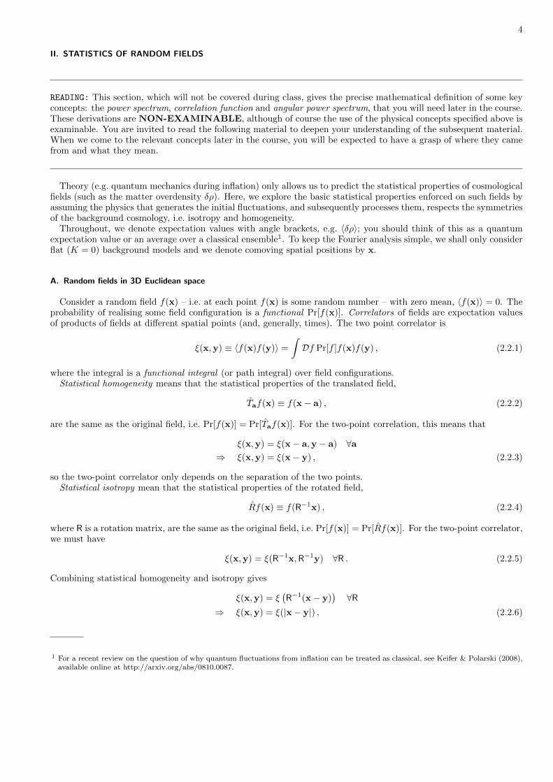
The real universe is far from homogeneous and isotropic except on the largest scales. Figure 1 shows slices throughthe 3D distribution of galaxy positions from the 2dF galaxy redshift survey out to a comoving distance of 600 Mpc.The distribution of galaxies is clearly not random; instead they are arranged into a delicate cosmic web with galaxiesstrung out along dense filaments and clustering at their intersections leaving huge empty voids. However, if wesmooth the picture on large scales (∼ 100 Mpc) it starts to look much more homogeneous. Furthermore, we knowfrom the CMB that the universe was smooth to around 1 part in 105 at the time of recombination; see Fig. 2.The aim of this part of the course is to study the growth of large-scale structure in an expanding universe throughgravitational instability acting on small initial perturbations. We shall then learn how these initial perturbations werelikely produced by quantum effects during cosmological inflation.

FIG. 1 Slices through the 3D map of galaxy positions from the 2dF galaxy redshift survey. Note that redshift 0.15 is at acomoving distance of 600 Mpc. Figure credit: 2dF.

FIG. 2 Fluctuations in the CMB temperature, as determined from five years of WMAP data, about the average temperatureof 2.725 K. The fluctuations are at the level of only a few parts in 105. Credit: WMAP science team.

A. Overview of structure formation

We will compute Pi(k), the initial power spectrum of density fluctuations, e.g. from inflation. The aim of this sectionis to understand how this initial spectrum is processed by the evolution of the universe, using linear perturbationtheory.

This processing is often quantified in terms of the transfer function:

δk(t0) = T (k)δk(ti)⇒ P (k) = T 2(k)Pi(k) . (2.1.1)

4

II. STATISTICS OF RANDOM FIELDS

READING: This section, which will not be covered during class, gives the precise mathematical definition of some keyconcepts: the power spectrum, correlation function and angular power spectrum, that you will need later in the course.These derivations are NON-EXAMINABLE, although of course the use of the physical concepts specified above isexaminable. You are invited to read the following material to deepen your understanding of the subsequent material.When we come to the relevant concepts later in the course, you will be expected to have a grasp of where they camefrom and what they mean.

Theory (e.g. quantum mechanics during inflation) only allows us to predict the statistical properties of cosmologicalfields (such as the matter overdensity δρ). Here, we explore the basic statistical properties enforced on such fields byassuming the physics that generates the initial fluctuations, and subsequently processes them, respects the symmetriesof the background cosmology, i.e. isotropy and homogeneity.

Throughout, we denote expectation values with angle brackets, e.g. 〈δρ〉; you should think of this as a quantumexpectation value or an average over a classical ensemble1. To keep the Fourier analysis simple, we shall only considerflat (K = 0) background models and we denote comoving spatial positions by x.

A. Random fields in 3D Euclidean space

Consider a random field f(x) – i.e. at each point f(x) is some random number – with zero mean, 〈f(x)〉 = 0. Theprobability of realising some field configuration is a functional Pr[f(x)]. Correlators of fields are expectation valuesof products of fields at different spatial points (and, generally, times). The two point correlator is

ξ(x,y) ≡ 〈f(x)f(y)〉 =

∫Df Pr[f ]f(x)f(y) , (2.2.1)

where the integral is a functional integral (or path integral) over field configurations.Statistical homogeneity means that the statistical properties of the translated field,

Taf(x) ≡ f(x− a) , (2.2.2)

are the same as the original field, i.e. Pr[f(x)] = Pr[Taf(x)]. For the two-point correlation, this means that

ξ(x,y) = ξ(x− a,y − a) ∀a⇒ ξ(x,y) = ξ(x− y) , (2.2.3)

so the two-point correlator only depends on the separation of the two points.Statistical isotropy mean that the statistical properties of the rotated field,

Rf(x) ≡ f(R−1x) , (2.2.4)

where R is a rotation matrix, are the same as the original field, i.e. Pr[f(x)] = Pr[Rf(x)]. For the two-point correlator,we must have

ξ(x,y) = ξ(R−1x,R−1y) ∀R . (2.2.5)

Combining statistical homogeneity and isotropy gives

ξ(x,y) = ξ(R−1(x− y)

)∀R

⇒ ξ(x,y) = ξ(|x− y|) , (2.2.6)

1 For a recent review on the question of why quantum fluctuations from inflation can be treated as classical, see Keifer & Polarski (2008),available online at http://arxiv.org/abs/0810.0087.

5

so the two-point correlator depends only on the distance between the two points. Note that this holds even ifcorrelating fields at different times, or correlating different fields.

We can repeat these arguments to constrain the form of the correlators in Fourier space. We adopt the symmetricFourier convention, so that

f(k) =

∫d3x

(2π)3/2f(x)e−ik·x and f(x) =

∫d3k

(2π)3/2f(k)eik·x . (2.2.7)

Note that for real fields, f(k) = f∗(−k). Under translations, the Fourier transform acquires a phase factor:

Taf(k) =

∫d3x

(2π)3/2f(x− a)e−ik·x

=

∫d3x′

(2π)3/2f(x′)e−ik·x

′e−ik·a

= f(k)e−ik·a . (2.2.8)

Invariance of the two-point correlator in Fourier space is then

〈f(k)f∗(k′)〉 = 〈f(k)f∗(k′)〉e−i(k−k′)·a ∀a

⇒ 〈f(k)f∗(k′)〉 = F (k)δ(k− k′) , (2.2.9)

for some (real) function F (k). We see that different Fourier modes are uncorrelated. Under rotations,

Rf(k) =

∫d3x

(2π)3/2f(R−1x)e−ik·x

=

∫d3x

(2π)3/2f(R−1x)e−i(R

−1k)·(R−1x)

= f(R−1k) , (2.2.10)

so, additionally demanding invariance of the two-point correlator under rotations implies

〈Rf(k)[Rf(k′)]∗〉 = 〈f(R−1k)f∗(R−1k′)〉 = F (R−1k)δ(k− k′) = F (k)δ(k− k′) ∀R . (2.2.11)

(We have used δ(R−1k) = detRδ(k) = δ(k) here.) This is only possible if F (k) = F (k) where k ≡ |k|. We cantherefore define the power spectrum, Pf (k), of a homogeneous and isotropic field, f(x), by

〈f(k)f∗(k′)〉 =2π2

k3Pf (k)δ(k− k′) . (2.2.12)

The normalisation factor 2π2/k3 in the definition of the power spectrum is conventional and has the virtue of makingPf (k) dimensionless if f(x) is.

The correlation function is the Fourier transform of the power spectrum:

〈f(x)f(y)〉 =

∫d3k

(2π)3/2

d3k′

(2π)3/2〈f(k)f∗(k′)〉︸ ︷︷ ︸

2π2

k3Pf (k)δ(k−k′)

eik·xe−ik′·y

=1

4π

∫dk

kPf (k)

∫dΩke

ik·(x−y) . (2.2.13)

We can evaluate the angular integral by taking x−y along the z-axis in Fourier space. Setting k · (x−y) = k|x−y|µ,the integral reduces to

2π

∫ 1

−1

dµ eik|x−y|µ = 4πj0(k|x− y|) , (2.2.14)

where j0(x) = sin(x)/x is a spherical Bessel function of order zero. It follows that

ξ(x,y) =

∫dk

kPf (k)j0(k|x− y|) . (2.2.15)

Note that this only depends on |x− y| as required by Eq. (2.2.6).The variance of the field is ξ(0) =

∫d ln kPf (k). A scale-invariant spectrum has P(k) = const. and its variance

receives equal contributions from every decade in k.

6

B. Gaussian random fields

For a Gaussian (homogeneous and isotropic) random field, Pr[f(x)] is a Gaussian functional of f(x). If we think ofdiscretising the field in N pixels, so it is represented by a N -dimensional vector f = [f(x1), f(x2), . . . , f(xN )]T , theprobability density function for f is a multi-variate Gaussian fully specified by the correlation function

〈fifj〉 = ξ(|xi − xj |) ≡ ξij , (2.2.16)

where fi ≡ f(xi), so that

Pr(f) ∝ e−fiξ−1ij fj√

det(ξij). (2.2.17)

Since f(k) is linear in f(x), the probability distribution for f(k) is also a multi-variate Gaussian. Since differentFourier modes are uncorrelated (see Eq. 2.2.9), they are statistically independent for Gaussian fields.

Inflation predicts fluctuations that are very nearly Gaussian and this property is preserved by linear evolution.The cosmic microwave background probes fluctuations mostly in the linear regime and so the fluctuations look veryGaussian (see Fig. 2). Non-linear structure formation at late times destroys Gaussianity and gives the filamentarycosmic web (see Fig. 1). Searching for primordial non-Gaussianity to probe departures from simple inflation is a veryhot topic but no convincing evidence for primordial non-Gaussianity has yet been found.

C. Random fields on the sphere

Spherical harmonics form a basis for (square-integrable) functions on the sphere:

f(n) =

∞∑l=0

l∑m=−l

flmYlm(n) . (2.2.18)

The Ylm are familiar from quantum mechanics as the position-space representation of the eigenstates of L2 = −∇2

and Lz = −i∂φ:

∇2Ylm = −l(l + 1)Ylm

∂φYlm = imYlm , (2.2.19)

with l an integer ≥ 0 and m an integer with |m| ≤ l. The spherical harmonics are orthonormal over the sphere,∫dnYlm(n)Y ∗l′m′(n) = δll′δmm′ , (2.2.20)

so that the spherical multipole coefficients of f(n) are

flm =

∫dn f(n)Y ∗lm(n) . (2.2.21)

There are various phase conventions for the Ylm; here we adopt Y ∗lm = (−1)mYl−m so that f∗lm = (−1)mfl−m for areal field.

What is the implication of statistical isotropy for the correlators of flm? For the two-point correlator, it turns outthat we must have2

〈flmf∗l′m′〉 = Clδll′δmm′ , (2.2.22)

2 A plausibility argument is as follows. Under rotations, the subset of the Ylm with a given l (so 2l + 1 elements) transforms irreduciblyso the δll′ form of the correlator is preserved under rotation. For rotation through γ about the z-axis,

Ylm(θ, φ)→ Ylm(θ, φ− γ) = e−imγYlm(θ, φ) ⇒ flm → e−imγflm .

Under rotations,

〈flmf∗l′m′ 〉 → e−imγeim′γ〈flmf∗l′m′ 〉 ,

so invariance requires the correlator be ∝ δmm′ .

7

where Cl is the angular power spectrum of f . What does this imply for the two-point correlation function? We have

〈f(n)f(n′)〉 =∑lm

∑l′m′

〈flmf∗l′m′︸ ︷︷ ︸Clδll′δmm′

〉Ylm(n)Y ∗l′m′(n′)

=∑l

Cl∑m

Ylm(n)Y ∗lm(n′)︸ ︷︷ ︸2l+14π Pl(n·n′)

= C(θ) , (2.2.23)

where n · n′ = cos θ and we used the addition theorem for spherical harmonics to express the sum of products of theYlm in terms of the Legendre polynomials Pl(x). It follows that the two-point correlation function depends only onthe angle between the two points, as required by statistical isotropy. Note that the variance of the field is

C(0) =∑l

2l + 1

4πCl ≈

∫d ln l

l(l + 1)Cl2π

. (2.2.24)

It is conventional to plot l(l + 1)Cl/(2π) which we see is the contribution to the variance per log range in l. Finally,we note that we can invert the correlation function to get the power spectrum by using orthogonality of the Legendrepolynomials:

Cl = 2π

∫ 1

−1

d cos θ C(θ)Pl(cos θ) . (2.2.25)

8

III. NEWTONIAN STRUCTURE FORMATION

Newtonian gravity is an adequate approximation of general relativity in cosmology on scales well inside the Hubbleradius and when describing non-relativistic matter (for which the pressure P is much less than the energy densityρ). Newtonian gravity underlies all cosmological N -body simulations of the non-linear growth of structure and ismuch more intuitive than the full linearised treatment of general relativity (to be introduced later). In particular, incosmology we can use the Newtonian treatment to describe sub-Hubble fluctuations in the cold dark matter (CDM)and baryons after decoupling.

Consider an ideal, self-gravitating non-relativistic fluid with density (for this section only, the mass density which,given our assumptions is essentially the total energy density) ρ, pressure P ρ and velocity u. Denote the usualNewtonian position vector by r and time by t. The equations of motion of the fluid are as follows:

Continuity ∂tρ+ ∇r · (ρu) = 0 (2.3.1)

Euler ∂tu + u ·∇ru = −1

ρ∇rP −∇rΦ (2.3.2)

Poisson ∇2rΦ = 4πGρ , (2.3.3)

where the gravitational potential Φ determines the gravitational acceleration by g = −∇rΦ. We can fudge the Poissonequation to get the correct Friedmann equations (see later) including the cosmological constant Λ by taking

∇2rΦ = 4πGρ− Λ . (2.3.4)

A. Background cosmology

To recover the background dynamics (described by the Friedmann equations), we consider a uniform expandingball of fluid satisfying Hubble’s law u = H(t)r. (Note the velocity goes to the speed of light at the Hubble radius!)This was covered in the third year cosmology course, but we include it again here from the perspective of the fluidequations.

Taking Φ = 0 at r = 0, the Poisson equation (2.3.4) integrates as

∂

∂r

(r2 ∂Φ

∂r

)= (4πGρ− Λ)r2

⇒ ∂Φ

∂r=

1

3(4πGρ− Λ)r

⇒ Φ =1

6(4πGρ− Λ)r2 . (2.3.5)

The Euler equation then becomes

∂H

∂tr +H2 r ·∇rr︸ ︷︷ ︸

r

= −1

3(4πGρ− Λ)r

⇒ ∂H

∂t+H2 =

1

3(Λ− 4πGρ) . (2.3.6)

This is the Newtonian limit of one of the Friedmann equations (the relativistic result replaces ρ with the sum of theenergy density and three times the pressure, ρ+ 3P ).

The continuity equation becomes

∂tρ+ ∇r · [ρ(t)H(t)r] = 0

⇒ ∂tρ+ 3ρH = 0 . (2.3.7)

This is the usual Friedmann statement of energy conservation for ρ P . Introducing the scale factor a via ∂ta/a = H,we have

1

ρ

∂ρ

∂t+

3

a

∂a

∂t= 0 ⇒ ρ ∝ a−3 , (2.3.8)

which describes the dilution of the mass density by expansion.

9

Equations (2.3.6) and (2.3.7) have a first integral

−K = a2

(H2 − 8πG

3ρ− 1

3Λ

). (2.3.9)

This is easily checked by differentiating:

−∂K∂t

= 2a2H

(H2 − 8πG

3ρ− 1

3Λ

)+ a2

(2H

∂H

∂t− 8πG

3

∂ρ

∂t

)= a2

[2H3 − 16πG

3Hρ− 2

3HΛ + 2H

(−H2 − 4πG

3ρ+

1

3Λ

)+ 8πGHρ

]= 0 . (2.3.10)

It follows that

H2 +K

a2=

1

3(8πGρ+ Λ) . (2.3.11)

In general relativity, K/a2 is 1/6 of the intrinsic curvature of the surfaces of homogeneity.

B. Comoving coordinates

A comoving observer in the background (i.e. unperturbed) cosmology has velocity dr/dt = H(t)r hence positionr = a(t)x where x is a constant. Rather than labelling events by t and r, it is convenient to use t and x, where x arecomoving spatial coordinates: x = r/a(t). Note these are Lagrangian coordinates in the background but not in theperturbed model.

Derivatives transform as follows: (∂

∂t

)r

=

(∂

∂t

)x

+

(∂x

∂t

)r

·∇x

=

(∂

∂t

)x

−H(t)x ·∇ , (2.3.12)

where we use ∇ to denote the gradient with respect to x at fixed t; and

∇r = a−1∇ . (2.3.13)

In what follows, ∂t should be understood as being taken at fixed x.

C. Perturbation analysis

We now perturb ρ, u and Φ about their background values:

ρ→ ρ(t) + δρ ≡ ρ(t)(1 + δ) (2.3.14)

P → P (t) + δP (2.3.15)

u→ a(t)H(t)x + v (2.3.16)

Φ→ Φ(x, t) + φ . (2.3.17)

Here, δ is the fractional overdensity in the fluid and φ the perturbed gravitational potential. Since, for a particle inthe fluid,

dr

dt=d(ax)

dt= aHx + a

dx

dt= u , (2.3.18)

we see that adx/dt = v, so the peculiar velocity v describes changes in the comoving coordinates of fluid elements intime (i.e. departures from the background Hubble flow).

10

The continuity equation (2.3.1) becomes (on using Eq. 2.3.12)

(1 + δ)∂tρ−Hρx ·∇δ + ρ∂tδ +ρ

a∇ · [(1 + δ)(aHx + v)] = 0 . (2.3.19)

Gathering terms that are zeroth, first and second-order in products of perturbed quantities gives

∂tρ+ 3ρH︸ ︷︷ ︸0th−order

+ (∂tρ+ 3ρH)δ + ρ∂tδ +ρ

a∇ · v︸ ︷︷ ︸

1st−order

+ρ

a(v ·∇δ + δ∇ · v)︸ ︷︷ ︸

2nd−order

= 0 . (2.3.20)

The background equation (2.3.7) sets the zero-order part to zero. In linear perturbation theory, we assume theperturbations are small enough (and their spatial derivatives) that we can ignore the second-order part, so that

∂tδ +1

a∇ · v = 0 . (2.3.21)

EXERCISE: Show that Eqs (2.3.2) and (2.3.3) linearise to

∂tv +Hv = − 1

aρ∇δP − 1

a∇φ (2.3.22)

∇2φ = 4πGa2ρδ . (2.3.23)

Scalar/vector decomposition

We can always decompose the vector v as

v = ∇v︸︷︷︸scalar part

+ v⊥︸︷︷︸vector part

, (2.3.24)

where ∇ · v⊥ = 0. It follows from Eq. (2.3.21) that the vector part of v does not lead to clumping of the matter.Since ∇ × v = ∇ × v⊥, v⊥ describes the vorticity of the fluid – recalling that ∇r = a−1∇, the physical vorticity∇r × u = a−1∇× v⊥. In linear theory, the scalar and vector parts decouple. For example, consider the (comoving)curl of the perturbed Euler equation (2.3.22),

∇× ∂tv = ∂t(∇× v⊥) = −H∇× v⊥ . (2.3.25)

It follows that ∇×v⊥ decays as 1/a in an expanding universe so the vorticity falls as 1/a2. This decay of the vorticityis consistent with the circulation theorem,

∮u · dr = const. for a path comoving with the fluid. For general initial

conditions, the peculiar velocity approaches a gradient at late times and the vector modes can be neglected. For initialconditions from inflation, vector modes are not excited in the first place. They are, however, important in modelswith continual sourcing of perturbations by cosmic defects.

D. Jeans’ length

The time derivative of the perturbed continuity equation (2.3.21) gives

∂2t δ −

1

aH∇ · v +

1

a∇ · ∂tv = 0. (2.3.26)

Combining with the perturbed Euler equation (2.3.22) and the Poisson equation (2.3.23), we find

∂2t δ −

1

aH∇ · v − 1

a∇ ·

(Hv +

1

aρ∇δP +

1

a∇φ

)= 0

⇒ ∂2t δ −

2

aH∇ · v − 1

a2ρ∇2δP − 1

a2∇2φ = 0

⇒ ∂2t δ + 2H∂tδ − 4πGρδ − 1

a2ρ∇2δP = 0 . (2.3.27)

11

This is the fundamental equation for the growth of structure in Newtonian theory. It shows the general competitionbetween infall by gravitational attraction – the 4πGρδ term – and pressure support, ∇2δP .

Consider a barotropic fluid such that P = P (ρ); then

δP =∂P

∂ρρδ ≡ c2sρδ (2.3.28)

where c2s is the sound speed. Using this in Eq. (2.3.27), and Fourier expanding so that ∇2 → −k2, gives

∂2t δ + 2H∂tδ +

(c2sk

2

a2− 4πGρ

)δ = 0 . (2.3.29)

This is the equation for a damped (in an expanding universe) oscillator provided that

c2sk2

a2> 4πGρ , (2.3.30)

and, in this case, the pressure support gives rise to acoustic oscillations (sound waves) in the fluid. However, forc2sk

2/a2 < 4πGρ, the system is unstable to gravitational accretion. Perturbations with proper wavelength 2πa/kexceeding the (proper) Jeans’ wavelength,

λJ ≡ cs√

π

Gρ, (2.3.31)

are gravitationally unstable, while on smaller scales pressure supports oscillations.For a fluid with equation of state P/ρ > −1/3, the proper Jeans’ length in an expanding universe grows faster

than a comoving scale (∝ a). This has the consequence that Fourier modes of the perturbations that start off outsidethe Jeans’ length, where they evolve by gravitational accretion, later come inside the Jeans’ length and subsequentlyundergo acoustic oscillations.

The Jeans’ length is roughly the radius R of a region of background density ρ such that the free-fall time, tff , equalsthe sound-crossing time, tsound. To see this, note that the free-fall time is the time to collapse under gravity. Considera shell of matter on the edge of a collapsing mass M of intitial radius R, such that at time t later the shell is atradius r. The mass enclosed is always M so that the gravitational acceleration is −GM/r2. Equating this to ∂2

t r,and solving for a particle initially at rest, the shell collapses to r = 0 in the free-fall time where

tff ∼R3/2

√GM

∼ 1√Gρ

. (2.3.32)

The sound-crossing time is simply tsound = R/cs and this equals the free-fall time for R ∼ cs/√Gρ ∼ λJ. Fluctuations

larger than the Jeans’ length do not have time for pressure to resist gravitational infall since the time to infall is lessthan the time it takes to propagate a pressure disturbance (i.e. a sound wave) across the perturbation. Note, finally,that the free-fall time is roughly the Hubble time, 1/H, when curvature and dark energy are negligible.

E. Applications to cold dark matter

1. Solutions in an Einstein-de Sitter phase

After matter-radiation equality, but well before dark energy comes to dominate, our universe is well described by anEinstein-de Sitter model having P ≈ 0 and zero curvature or Λ. Scales of cosmological interest are much larger thanthe Jeans’ scale for the baryons and so both CDM fluctuations and those for the baryons have the same dynamicalequations. We shall show shortly that quickly after recombination, the fractional overdensity in the baryons, δb,approaches that in the CDM, δc, and the matter behaves like a single pressure-free fluid with total density contrast

δm =ρbδb + ρcδcρb + ρc

≈ δc . (2.3.33)

Since H2 ∝ ρ ∝ a−3, we have a ∝ t2/3 and so H = 2/(3t) and 4πGρ = 2/(3t2). Equation (2.3.27) then gives theevolution of the density fluctuations in the pressure-free matter as

∂2t δm +

4

3t∂tδm −

2

3t2δm = 0 . (2.3.34)

12

Trying solutions like tp gives independent solutions δm ∝ t−1 and δm ∝ t2/3 ∝ a. The growing-mode solution ofthe density contrast therefore grows like the scale factor. Note that here, in an expanding universe, gravitationalattraction has given rise to power-law growth of δ to be compared to the exponential growth predicted in a non-expanding model. The Poisson equation (2.3.23) tells us that the gravitational potential is constant since, in Fourierspace,

−k2φ = 4πGa2 ρ︸︷︷︸∝a−3

δ︸︷︷︸∝a

= const. (2.3.35)

2. The Meszaros effect

The Meszaros effect describes the way that CDM grows only logarithmically on scales inside the sound horizonduring radiation domination. Generally, CDM (or anything else) feels the gravity of all clustered components soEq. (2.3.27) generalises to the ith component of a set of non-interacting (except through gravity) fluids as

∂2t δi + 2H∂tδi − 4πG

∑j

ρjδj −1

a2ρi∇2δPi = 0 . (2.3.36)

Specialising to pressure-free CDM we have

∂2t δc + 2H∂tδc − 4πG

∑j

ρjδj = 0 . (2.3.37)

Our Newtonian treatment at least makes it plausible that the Jeans’ length for perturbations in the radiation fluid(for which cs = 1/

√3) during radiation domination is of the order of the Hubble radius. Radiation fluctuations on

scales smaller than this therefore oscillate as sound waves and their time-averaged density contrast vanishes (we shallshow this properly when we develop relativistic perturbation theory). It follows that the CDM is essentially the onlyclustered component during the acoustic oscillations of the radiation, and so

∂2t δc +

1

t∂tδc − 4πGρcδc = 0 , (2.3.38)

where we used a ∝ t1/2 and so H = 1/(2t). Since δc evolves only on cosmological timescales (it has no pressuresupport for it to do otherwise),

∂2t δc ∼ H2δc 4πGρcδc (2.3.39)

during radiation domination, as ρr ρc. We can therefore ignore the last term in Eq. (2.3.38) compared to theothers and we have solutions with δc = const. and δc ∝ ln t. We see that the rapid expansion due to the effectivelyunclustered radiation reduces the growth of δc to only logarithmic.

3. Late-time suppression of structure formation by Λ

At late times, the dominant clustered component is the matter and we have

∂2t δm + 2H∂tδm − 4πGρmδm = 0 . (2.3.40)

In matter domination, this reduces to Eq. (2.3.34) and δm grows like a, but when Λ comes to dominate a ∝ et√

Λ/3

and H ≈ const. It follows that 4πGρm H2 (currently 4πGρm/H2 ∼ 0.37) and

∂2t δm + 2H∂tδm ≈ 0 . (2.3.41)

The solutions of this are δm = const. or δm ∝ e−2t√

Λ/3 ∝ a−2 and Λ suppresses the growth of structure. Note alsothat a constant density contrast implies that the gravitational potential decays as a2ρm ∝ a−1. This leaves an imprintin the CMB called the integrated Sachs-Wolfe effect.

13

FIG. 3 Ratio of the matter power spectrum to a smooth spectrum (i.e. a model with no baryons) showing the expected baryonacoustic oscillations. Credit: Percival et al.

4. Evolution of baryon fluctuations after decoupling

Before decoupling, the baryon dynamics is linked to that of the radiation by efficient (Compton) scattering. Onsub-Hubble scales, δb oscillates like the radiation but, after matter-radiation equality, δc grows like a. It follows thatjust after decoupling, δc δb. Subsequently, the baryons fall into the potential wells sourced mainly by the CDMand δb → δc as we shall now show.

Ignoring baryon pressure and Λ, the coupled dynamics of the baryon and CDM fluids after decoupling is approxi-mately given by

∂2t δb +

4

3t∂tδb = 4πG(ρbδb + ρcδc) (2.3.42)

∂2t δc +

4

3t∂tδc = 4πG(ρbδb + ρcδc) . (2.3.43)

We can decouple these equations by using normal coordinates δm (see equation 2.3.33) and ∆ ≡ δc − δb. Then

∂2t ∆ +

4

3t∂t∆ = 0 ⇒ ∆ = const. or ∆ ∝ t−1/3 , (2.3.44)

while δm follows Eq. (2.3.34) and has solutions ∝ t−1 and t2/3. Since

δcδb

=ρmδm + ρb∆

ρmδm − ρc∆→ δm

δm= 1 , (2.3.45)

we see that δb approaches δc.The non-zero initial value of δb at decoupling, and, more importantly ∂tδb, leaves a small imprint in the late-time δm

that oscillates with scale. These baryon acoustic oscillations have recently been detected in the clustering of galaxies(see Fig. 3).

14

IV. RELATIVISTIC STRUCTURE FORMATION

This section will be done entirely on the whiteboard.

V. INFLATION AND THE ORIGIN OF STRUCTURE

A. Schematic overview of origin of structure in the inflationary paradigm

So far, we have not discussed the origin of the primordial perturbation which provided the seeds for cosmologicalstructure formation under the action of gravitational instability. The study of this question has the potential to exposedeep connections between cosmology and physics at immensely high energies which are forever beyond the reach ofearth-bound particle accelerators.

Besides solving the big bang puzzles, the decreasing comoving horizon during inflation is the key feature requiredfor the quantum generation of cosmological perturbations. During inflation, quantum fluctuations are generated onsub-Hubble scales and are then stretched out of the Hubble radius by the accelerated expansion. In other words,the superluminal expansion stretches the perturbations to apparently acausal distances. They become classical su-perhorizon density perturbations which re-enter the Hubble radius in the subsequent non-accelerating evolution andthen undergo gravitational collapse to form the large-scale structure in the universe.

We are most interested in the scalar perturbations to the metric, as these couple to the density of matter andradiation, and are ultimately responsible for most of the inhomogeneities and anisotropies in the universe. In addi-tion to scalar perturbations, however, inflation also generates tensor fluctuations in the gravitational metric (calledgravitational waves). These are not coupled to the density and thus are not responsible for the large-scale structureof the universe. However, they do induce fluctuations in the cosmic microwave background (CMB). In fact, thesefluctuations turn out to be a unique signature of inflation and offer the best window on the physics driving inflation.

We will study tensor perturbations before scalar perturbations for reasons of simplicity. Tensor perturbations tothe metric due to a scalar field are not coupled to any other perturbation variables, so when we consider them, we arelooking at the fluctuations in a single field. Scalar perturbations to the metric couple to energy density fluctuations.The coupled fields fluctuate together and complicate the maths. This distracts from the main point, which is thatquantum mechanical fluctuations during inflation are responsible for the perturbations around the smooth backgroundthat ultimately gives rise to all the structure in universe. So we will first introduce this idea in the simplified contextof a single field, and start with tensor perturbations.

During inflation, the universe consists primarily of a uniform scalar field and a uniform background metric. Againstthis background, the fields fluctuate quantum mechanically. Perturbations of the inflaton field value δφ satisfythe equation of motion of a harmonic oscillator with time-dependent mass. The quantum treatment of inflatonperturbations therefore parallels the quantum treatment of a collection of one-dimensional harmonic oscillators. Justas zero-point fluctuations of a harmonic oscillator induce a non-zero variance for the oscillation amplitude 〈x2〉, thequantum fluctuations of a light scalar field3 during inflation induce a non-zero variance for the inflaton perturbations.Our goal is to compute this variance and see how it evolves as inflation progresses. Once we know this variance, wecan draw from a distribution with this variance to set the initial conditions.

B. Quantizing the harmonic oscillator

In order to compute the quantum fluctuations in the metric, we need to quantize the field. For both scalar andtensor perturbations, the easiest way to do this is to rewrite the problem so that it looks like a simple harmonicoscillator (SHO).

Let us remind ourselves a few facts about the quantization of an SHO.

• An SHO with unit mass and frequency ω obeys

x+ ω2x = 0 . (2.5.1)

• Upon quantitization, x becomes a quantum operator

x = v(ω, t)a+ v∗(ω, t)a† (2.5.2)

3 Such a field has (effective) mass V,ΦΦ H2 which is equivalent to |ηV | 1.

15

where a is a quantum operator and v ∝ exp(iωt) is a solution to the SHO equation (2.5.1).

• The operator a annihilates the vacuum state, a|0〉 = 0 (in which there are no particles) and satisfies thecommutation relation

[a, a†] ≡ aa† − a†a = 1 , (2.5.3)

giving variance

〈|x|2〉 ≡ 〈0|x†x|0〉 = |v(ω, t)|2. (2.5.4)

EXERCISE: If you need to refresh your memory for quantization of the SHO, read Sec. 6.4.1. in Dodelson.

C. Tensor perturbations

Tensor perturbations are characterized by a metric with g00 = 1, zero space-time components g0i = 0, and spatialelements

gij = −a2

1 + h+ h× 0h× 1− h+ 00 0 1

. (2.5.5)

That is, the perturbations to the metric are described by two functions h+ and h×, assumed small. For definiteness,we have chosen the perturbations to be in the x–y plane. This corresponds to an implicit choice of axes; in particular

it corresponds to choosing the z axis to be in the direction of the wavevector ~k.More generally, h+ and h× are two components of a divergenceless, traceless, symmetric tensor. If this perturbation

tensor is written as Hij , divergenceless means that kiHij = kjHij = 0. This is clearly satisfied by (2.5.5) since there

are no components in the k = z direction. Tracelessness is also satisfied since the sum of perturbations along thediagonal vanishes.

Once the metric has been written down, we know what to do - the procedure is identical to what we used in Part Iof the course to derive the Einstein equations for the unperturbed metric. The derivation proceeds as usual in threesteps: (i) Christoffel symbols, (ii) Ricci tensor, and (iii) Ricci scalar.

EXERCISE: Work through the GR machinery with the aid of Sec. 5.3 of Dodelson. The minimum learning outcomeof this exercise should be to understand every step of this derivation, even if you ultimately can’t reproduce it withthe book closed.

During inflation, gravitational waves are not sourced by the scalar field – i.e. perturbing the energy-momentumtensor of a scalar field leads to a zero RHS in the relevant perturbed Einstein equation (see Exercise 10 in Chapter 6of Dodelson). The perturbed Einstein equation thus leads to

h′′α + 2

(a′

a

)h′α + k2hα = 0 , (2.5.6)

where α = +,× and primes denote derivatives with respect to conformal time η. Eq. (2.5.6) is a wave equation, andthe corresponding solutions are called gravitational waves. For example, if we neglect the expansion of the universeso that the damping term in (2.5.6) vanishes, the equation is manifestly in the form of an SHO equation and weimmediately see that the two solutions are hα ∝ e±ikη. In real space, the perturbation to the metric is in the form

hα(~x, η) =

∫d3k

(2π)3/2ei~k·~x [Aeikη +Be−ikη

](no expansion) . (2.5.7)

16

These two modes correspond to waves travelling in the ±z direction at the speed of light. Eq. (2.5.6) is a generalizationof the wave equation to an expanding universe.

EXERCISE: Solve the wave equation (2.5.6) if the universe is purely matter-dominated. Do the same for the radiation-dominated case.

FIG. 4 Evolution of gravitational waves as a function of conformal time. Three different modes are shown, labelled by theirwavenumbers. Smaller scale modes decay earlier. Figure credit: Modern Cosmology, Dodelson.

The solutions are oscillatory, like the simple ones in (2.5.7), but also damp out. Fig. 4 shows the evolution of hαfor three different wavelength modes. The large scale mode (with kη0 = 10) remains constant at early times when itswavelength is larger than the horizon, kη < 1. Once its wavelength becomes comparable to the horizon, kη ∼ 1, thesolution oscillates several times until the present epoch and the amplitude begins to die off. The small scale modekη0 = 1000 illustrated here also begins to decay when its wavelength becomes comparable to the horizon. Its horizonentry occurs much earlier, though, so the decay is much more efficient, and by today, its amplitude is extremely small.

An important point about the effect of gravity waves on the CMB anisotropy spectrum can be gleaned from thisdiscussion. Because small-scale modes decay earlier than large scale modes, at decoupling (at η/η0 ' 0.02) only modeswith kη0 & 100 persist. All smaller scale modes can be neglected. Therefore, anisotropies on small angular scales willnot be affected by gravitational waves. Only the large-scale anisotropies are affected.

Now let us return to eq. (2.5.6). To continue with our programme of parsimoniously re-using the previous knowledgeon quantizing the SHO, we would like to massage this equation into the form of a SHO, so that h can be easilyquantized.

To do this, define

h ≡ ah√16πG

, (2.5.8)

where we have cunningly normalized the field to match the canonical normalization of a scalar field4. Working through

4 If you are interested in this normalization factor, read the footnote at the bottom of pp158 in Dodelson.

17

the maths of substituting this redefinition into (2.5.6), we arrive at:

h′′ +

(k2 − a′′

a

)h = 0 . (2.5.9)

EXERCISE: Complete the missing steps to change the variable in (2.5.6) to arrive at (2.5.9).

We have now arrived at the form of an SHO, which we know how to use! The equation now has no damping term(∝ h′) so we can immediately write down an expression for the quantum operator

ˆh(~k, η) = v(k, η)a~k + v∗(k, η)a†~k

, (2.5.10)

where the coefficients of the creation and annihilation operators satisfy the equation

v′′ +

(k2 − a′′

a

)v = 0 . (2.5.11)

Further, we know the variance of the perturbations

〈ˆh†(~k, η)

ˆh(~k′, η)〉 = |v(k, η)|2δ3(~k − ~k′) . (2.5.12)

After transforming back to the h field, we see that

〈h†(~k, η)h(~k′, η)〉 =16πG

a2|v(~k, η)|2δ3(~k − ~k′) ,

≡ 2π2

k3Ph(k)δ3(~k − ~k′) (2.5.13)

where the second line defines the power spectrum of the primordial perturbations to the metric. Note that conventionsabound in the definition of the primordial power spectrum. We have followed the usual early universe communitydefinition which gives a dimensionless power spectrum. Dodelson follows the convention of the large scale structurecommunity where the power spectrum is taken to have dimensions of k−3. Further, Dodelson is using a different Fourierconvention to this class, and we use the one which is more conventional in the field. If you find this frustrating, youare not alone.

Thus, with this definition, we have

Ph(k) = 16πG

(k3

2π2

)|v(k, η)|2

a2. (2.5.14)

To determine the spectrum of tensor perturbations produced during inflation, we have to now solve the second orderdifferential equation (2.5.16) for v(k, η).

EXERCISE: Show that, during inflation, (a′′

a

)' 2

η2. (2.5.15)

.

The relevant equation therefore becomes

v′′ +

(k2 − 2

η2

)v = 0 . (2.5.16)

18

The initial conditions necessary to solve this equation come from considering v at very early times before inflation hasdone most of its work. At that time, −η is large, of order ηprim, so the k2 term dominates, and the equation reduces

precisely to that of the SHO. In that case, we know that the properly normalized solution is e−ikη/√

2k. The solutionwhich correctly yields this limit is

v =e−ikη√

2k

[1− i

kη

]. (2.5.17)

This obviously goes into the correct solution when the mode is well within the horizon (k|η| 1).

EXERCISE: Check that (2.5.17) is a solution of (2.5.16).

The evolution of a mode h with wavenumber k according to this solution can be interpreted as follows. When themode is well within the horizon (k|η| 1), the amplitude of h decays as h ∝ 1/a ,

v → e−ikη√2k

=⇒ h ∝ 1

ak|η| 1 . (2.5.18)

At kη = 1, the mode leaves the horizon. Well outside the horizon, (−kη → 0), h becomes constant:

v → e−ikη√2k

i

kη=⇒ h→ const − kη → 0 . (2.5.19)

The primordial power spectrum for tensor modes, which scales as |v|2/a2, is thus constant after the mode exits thehorizon. This constant determines the initial conditions with which to start off h×,+ at early times. Here, “early”means well after inflation has ended but before decoupling. The primordial power spectrum for tensor modes is then

Ph(k) =16πG

a2

(k3

2π2

)1

2k3η2

' 16πG

(H

2π

)2

. (2.5.20)

We have assumed H is constant in deriving the last line. Specifically, during slow-roll inflation the fractional variationin the Hubble rate per Hubble time is small so we can treat H as a constant, Hk, for the few e-folds either side ofHubble exit. Then, in this interval, a = −(Hkη)−1. More generally, H has to be evaluated at the time when themode of interest leaves the horizon. Since H ∼ constant during inflation, Ph is nearly scale-invariant. Our expressionalso implies that the detection of primordial gravitational waves measures the Hubble rate during inflation! Since theHubble rate is dominated by potential energy during inflation, we would also measure V (φ) at horizon exit!

Further, the fluctuations in h are Gaussian, just like the quantum-mechanical fluctuations of the SHO. Gaussianityis a fairly robust prediction of inflation (and thus, a means of testing the inflationary picture observationally). Finally,Eq. (2.5.20) is the power spectrum for h+ and h× separately, and each polarization contributes twice to the metricperturbations; these are uncorrelated, so the power spectrum for all modes must be multiplied by a factor of 4. Thus,we finally obtain the tensor power spectrum for inflation:

Ph = 64πG

(H

2π

)2

≡ 8

M2Pl

(H

2π

)2

. (2.5.21)

D. Scalar perturbations

A pedagogical treatment of the generation of density (scalar) perturbations is beyond the scope of this course andwe direct the interested reader to the comprehensive treatment in Kinney5 (2009). The quantity we wish to compute

5 http://arxiv.org/abs/0902.1529

19

is the comoving curvature perturbation R, since this is conserved from Hubble exit during inflation to Hubble re-entry during the standard radiation or matter-dominated epochs. With R we can reliably compute the primordialfluctuation (in single-field models of inflation) in the radiation era without needing to model the dynamics of thereheating process.

Let’s decompose the scalar field into a zero-order homogeneous part and a perturbation:

φ(~x, t) = φ(0)(t) + δφ(~x, t) , (2.5.22)

and find an equation governing δφ assuming the smoothly expanding FRW metric. Under this assumption, only firstorder pieces are perturbations to Tµν , and after the usual Einstein equation manipulations, we find

δφ′′ + 2a′

aδφ′ + k2δφ = 0 . (2.5.23)

This equation has the same form as the tensor case (2.5.6), and we can trivially copy the solution, dropping the tensornormalization factor 16πG as we already have a canonical scalar field:

Pδφ =

(H

2π

)2

. (2.5.24)

The right-hand side is evaluated when the mode k exits the Hubble radius. Since H varies very slowly duringinflation, the scalar power spectrum is also nearly (but not exactly) scale-invariant. This is one of the most genericand important observational predictions of inflation.

In order to sketch how fluctuations in φ get transferred into density fluctuations, we will work in the ConformalNewtonian gauge (CNG), where the perturbed FRW metric is:

ds2 = a2(η)[(1 + 2Ψ)dη2 − δij(1− 2Φ)dxidxj ] . (2.5.25)

This metric describes scalar metric perturbations6 using the scalar potentials Ψ (Newtonian potential) and Φ (per-turbation to the spatial curvature).

We want to know how fluctuations in φ get transferred to Ψ (or Φ, assumed identical in magnitude here7) so that wecan relate inflationary perturbations to initial density fluctuations. We can then use the transfer functions derived inthe previous section to evolve them forward in time to any epoch after inflation ends, and compare with observations.

Until now, we have neglected the metric perturbations. When the wavelength of the perturbation is of the order ofthe horizon or smaller, this approximation is valid. However, by the end of inflation, the metric perturbation becomesimportant. Although the inflation-induced perturbations start off as all-δφ, they end up as a linear combination ofΨ and δφ, or more generally, as a linear combination of Ψ and perturbations to the energy momentum tensor. Thetrick is to find the linear combination which is conserved outside the horizon. The value of this conserved linearcombination is determined by δφ at horizon crossing. We can then evaluate it after inflation solely in terms of Ψ.Finding the linear relation between Ψ and δφ will immediately allow us to obtain PΨ in terms Pδφ obtained above.

The easiest way to do this is to switch to a gauge where the spatial part of the metric is unperturbed: a spatiallyflat slicing8. In such a gauge, the previous result (2.5.24) is exact. Now, the question is how to move back to theCNG. The answer is that we need to (i) find a gauge invariant variable ∝ δφ in a spatially flat slicing (SFS), and (ii)find this variable in CNG, thus linking Φ in CNG with δφ in SFS.

READING: (NON-EXAMINABLE) You can see these steps fleshed out on §6.5.3 (pp 169) of Dodelson. Though itsounds gory, it is a compact and elegant calculation.

In the SFS, the line element (with A, B characterizing the line element) is given by

ds2 = (1 + 2A)dt2 + 2aB,idxidt− δija2dxidxj . (2.5.26)

6 By the Decomposition Theorem, scalars, vectors and tensors evolve independently. Only scalars couple to matter.7 This assumption is equivalent to neglecting anisotropic stresses in the energy-momentum tensor.8 Technically, the field fluctuation here is defined on hypersurfaces with zero intrinsic curvature and, in this gauge, the result is the same

as if metric perturbations (i.e. the back-reaction of δφ on the spacetime geometry) were ignored.

20

It turns out that the appropriate gauge-invariant combo that translates between the two gauges is the previously-heralded comoving curvature perturbation,

R = − aH

∂ηφ(0)δφ , (2.5.27)

immediately giving us the power spectrum,

PR =

(aH

∂ηφ(0)

)2

Pδφ ≡(

H

∂tφ(0)

)2(H

2π

)2

≡(

H2

2π∂tφ(0)

)2

. (2.5.28)

The right hand side is again evaluated at horizon exit, k = aH.During inflation, comoving hypersurfaces have the property that they coincide with the hypersurfaces over which

the (total) inflaton φ is homogeneous. These hypersurfaces are not the same as the zero-curvature surfaces on whichEq. (2.5.24) holds – there is a time delay between them, δt = −δφ/∂tφ(0), such that the evolution of the backgroundφ(0) in this time compensates for the perturbation δφ to give a smooth total φ. The differential background expansionduring this time delay means that the intrinsic curvature of the comoving hypersurfaces is simply R = −Hδφ/∂tφ(0).This is reason for the curvature perturbation designation.

E. Slow-roll expansion

In this section, to avoid cumbersome notation we set Φ ≡ φ(0). For a slowly-rolling scalar field, we can expressPR(k) directly in terms of the inflaton potential. During slow roll, the potential energy of the field dominates overthe kinetic energy and so

H2 ≈ 1

3M2Pl

V (Φ) , (2.5.29)

and the field evolution is friction limited:

3H∂tΦ = −V,Φ(Φ) . (2.5.30)

(See the slow roll conditions.) It follows that

PR(k) =

(H2

2π∂tΦ

)2

≈(

3H3

2πV,Φ

)2

≈ (V/M2Pl)

3

3(2π)2(V,Φ)2

=8

3

(V 1/4

√8πMPl

)41

εV, (2.5.31)

where, recall, εV is the slow-roll parameter

εV ≡M2

Pl

2

(V ′

V

)2

. (2.5.32)

The large-angle CMB observations constrain PR(k) ∼ 2× 10−9 on current Hubble scales. It follows that

V 1/4 ∼ 6× 1016ε1/4V GeV . (2.5.33)

The quantity V 1/4 describes the energy scale of inflation and, since εV 1, the energy scale is at least two orders ofmagnitude below the Planck scale (∼ 1019 GeV). It is, however, plausible, that inflation occurred around the GUTscale, ∼ 1016 GeV.

F. Spectral index of the primordial power spectrum

We have already noted that slow-roll inflation produces a spectrum of curvature perturbations that is almost scale-invariant. We can quantify the small departures from scale-invariance by forming the spectral index ns(k). Generally,this is a scale-dependent quantity defined by

ns(k)− 1 ≡ d lnPR(k)

d ln k, (2.5.34)

21

where the −1 is conventional and (unfortunately!) means that a scale-free spectrum has ns = 1. For a constant ns,this definition implies a power-law spectrum

PR(k) = As(k/kpivot)ns−1 (2.5.35)

for some pivot scale kpivot.We can evaluate ns by noting that

d

d ln k=

dt

d ln k

dΦ

dt

d

dΦ, (2.5.36)

and, since k = aH at Hubble exit,

d ln k

dt= H

(1 +

∂tH

H2

). (2.5.37)

The Friedmann equation, and the slow-roll approximation then gives

∂tH

H2= −3

2

(ρ+ P

ρ

)≈ −3

2

(∂tΦ)2

V

= −1

2

(3H∂tΦ)2

3H2V

≈ −M2Pl

2

(V,ΦV

)2

= −εV , (2.5.38)

so that d ln k/dt ≈ H(1− εV ). We thus have, to leading-order in the slow-roll parameters,

d

d ln k≈ 1

H

dΦ

dt

d

dΦ

≈ −V,Φ3H2

d

dΦ

≈ −M2Pl

V,ΦV

d

dΦ

≈ −MPl

√2εV

d

dΦ. (2.5.39)

We can now differentiate Eq. (2.5.31) to find

ns − 1 = −MPl

√2εV

d

dΦ(lnV − ln εV )

= −MPl

√2εV

(V,ΦV−εV ,ΦεV

). (2.5.40)

The derivative of εV is

d ln εVdΦ

= 2

(V,ΦΦ

V,Φ−V,ΦV

)≈√

2

MPl

(ηV√εV− 2√εV

), (2.5.41)

where ηV is the slow-roll parameter related to the curvature of the potential previously defined in the first part of thecourse. This gives the final, simple result

ns(k)− 1 = 2ηV (Φ)− 6εV (Φ) . (2.5.42)

We see that departures from scale-invariance are first order in the slow-roll parameters. It can be shown thatdns/d ln k is second-order in slow roll so a power-law primordial power spectrum is a very good approximation forslow-roll inflation.

22

In this simple class of inflation models, the power spectrum of R is thus

PR(k) =

(H2

2π∂tΦ

)2

k=aH

≈

(V 3

12π2V 2,Φ

)k=aH

, (2.5.43)

where the second equality uses the slow-roll approximations. The efficiency of this mechanism for producing cosmo-logical curvature perturbations depends on both the height of the potential, which determines the expansion rate andhence size of δφ, and its slope, which enters through the conversion of inflaton fluctuations to time delays and socurvature.

Gravitational waves are a direct probe of the Hubble rate during inflation, or, using the slow-roll approximation,

Ph(k) ≈ 128

3

(V 1/4

√8πMPl

)4

, (2.5.44)

of the energy scale. Note that

r ≡ Ph(k)

PR(k)≈ 16εV , (2.5.45)

which defines the dimensionless tensor-to-scalar ratio r.The spectrum of gravitational waves is almost scale-invariant with a spectral index

nt ≡d lnPh(k)

d ln k≈ d lnV

d ln k= −MPl

√2εV

V,ΦV

= −MPl

√2εV

√2εVMPl

= −2εV . (2.5.46)

Note that this is always negative (the spectrum is said to be red) which is a direct consequence of the Hubbleparameter falling as inflation proceeds. It follows that r ≈ −8nt in slow-roll inflation which is an example of aslow-roll consistency relation between the spectra of curvature perturbations and gravitational waves.

G. Observable predictions and current observational constraints

The inflationary proposal requires a huge extrapolation of the known laws of physics. In the absence of a completetheory, a phenomenological approach has been commonly employed, where an effective potential V (φ) is postulated.Ultimately, V (φ) has to be derived from a fundamental theory, and significant progress in implementing inflation instring theory has been made in recent years. However, while it is challenging to understand the origin of inflationfrom a particle physics point of view, it is also a great opportunity to learn about ultra-high-energy physics fromcosmological observations.

The simplest inflationary scenarios consist of a single light scalar field with a canonical kinetic term, (∇φ)2/2, inits action. They predict the following observable characteristics.

1. Flat geometry, i.e. the observable universe should have no spatial curvature. As we have seen, flatness has beenverified at the 1% level by the location, or, better, separation, of the CMB acoustic peaks combined with somelow-redshift distance information.

2. Gaussianity, i.e. the primordial perturbations should correspond to Gaussian random variables to a very highprecision.

3. Scale-invariance, i.e. to a first approximation, there should be equal power at all length-scales in the perturbationspectrum, without being skewed towards high or low wavenumbers. In terms of the parameterisation above, thiscorresponds to ns = 1 and nt = 0. However, small deviations from scale-invariance are also a typical signatureof inflationary models and tell us about the dynamics of inflation.

4. Adiabaticity, i.e. after reheating, there are no perturbations in the relative number densities of different specieson super-Hubble scales. (so no isocurvature modes). This follows from the assumption that only a single fieldis important during inflation.

23

5. Super-Hubble fluctuations, i.e. there exist correlations between anisotropies on scales larger than the apparentcausal horizon, beyond which two points could not have exchanged information at light-speed during the historyof a non-inflationary universe. This corresponds to angular separations on the sky larger than ∼ 2.

6. Primordial gravitational waves, which give rise to temperature and polarization anisotropies. These tensormodes must exist; however, their predicted amplitude can vary by many orders of magnitude depending on theunderlying microphysical mechanism implementing inflation.

Please see the handout for a summary of the current observational evidence for inflation.

VI. THE COSMIC MICROWAVE BACKGROUND

Separate notes will be provided for this section.

24

VII. THE MATTER POWER SPECTRUM

The power spectrum of the late-time distribution of matter is a key cosmological observable. It can be estimatedin galaxy surveys by assuming that the fractional fluctuations in the number density of galaxies traces (generally ina biased manner) the fractional fluctuations in the matter.

Consider the fractional matter overdensity in the comoving gauge well after recombination, ∆m(η,k). The matterpower spectrum P∆m

(η; k) is then defined by

〈∆m(η,k)∆∗m(η,k′)〉 ≡ 2π2

k3P∆m

(η; k)δ(k− k′) . (2.5.47)

The power spectrum P∆m(η; k) is dimensionless, but frequently a dimensional spectrum P∆m

(η; k) is used, where

P∆m(η; k) ≡ 2π2

k3P∆m

(η; k) . (2.5.48)

One may also meet real-space measures of matter clustering, such a σR. This is defined to be the (real-space) varianceof ∆m averaged in spheres of radius R. This is equivalent to the variance of ∆m convolved with 3Θ(R− |x|)/(4πR3),i.e. a normalised spherical top-hat of radius R. The Fourier transform of such a top-hat is W (kR), where

W (x) ≡ 3

x3(sinx− x cosx) . (2.5.49)

From the convolution theorem, the variance of the convolved field is

σ2R =

∫d3k

(2π)3W 2(kR)P∆m(k) . (2.5.50)

Historically, a scale R = 8h−1 Mpc is chosen, where the Hubble constant H0 = 100h km s−1 Mpc−1, since σ8 ∼ 1.The smoothing scale at which the variance of a low-pass-filtered field exceeds unity — here ∼ 8h−1 Mpc — marksthe scale at which perturbation theory breaks down and non-linear effects become important. In the best-fit modelto the WMAP CMB data, σ8 ≈ 0.80.

FIG. 5 The matter power spectrum P∆m(k) at z = 0 in linear theory (solid) and with non-linear corrections (dashed). Credit:A. Challinor

The theoretical matter power spectrum at z = 0 is plotted in Fig. 5 based on linear perturbation theory. Alsoplotted is a fit to the results of N -body simulations that takes account of the non-linear growth of the density fieldon small scales. The main features of this plot are as follows.

25

• On large scales, P∆m(k) grows as k.

• The power spectrum turns over around k ∼ 0.01 Mpc−1 corresponding to the horizon size at mattter-radiationequality.

• Beyond the peak, the power falls as k−3 ln2(k/keq), where keq is the wavenumber of a mode that enters thehorizon at the matter-radiation transition.

• There are small amplitude baryon acoustic oscillations in the spectrum (see also Fig. 3).

• Linear theory applies on scales k−1 > 10 Mpc at z = 0.

The shape of the matter power spectrum as inferred from galaxy clustering agrees well with the theoretical predictionin Fig. 5. Inferring the amplitude is more problematic due to the issue of galaxy bias noted above.

To understand the shape of the matter power spectrum, we note that on scales where linear perturbation theoryholds we can write (for adiabatic initial conditions)

∆m(η,k) = T (η, k)R(0,k) , (2.5.51)

where T (η, k) is the transfer function which relates the primordial curvature perturbation to the comoving matterperturbation. The primordial curvature power spectrum is almost scale-free (P∆m

(0; k) ≈ const.; see Sec. V) soit contributes a factor of k−3 to P∆m

(k). This primordial shape is modified by the transfer function whose scaledependence results from the physics of structure formation.

First consider modes with k < keq. These were outside the horizon throughout radiation domination. For these,it turns out to be simplest to consider the Newtonian-gauge potential Φ: during matter domination Φ(η,k) =−3R(0,k)/5 for k < keq. The potential is suppressed uniformly on all scales when Λ comes to dominate, so thatΦ(η,k)/R(0,k) remains independent of k. We can relate ∆m to Φ via the Poisson equation which, in Fourier space,gives ∆m ∼ k2Φ. It follows that

T (η, k) ∝ k2 k < keq , (2.5.52)

and so P∆m(k) ∝ k4/k3 ∝ k on large scales.

For k > keq, the mode entered the horizon during radiation domination. Generally, on sub-Hubble scales, thedensity contrast in the comoving and Newtonian gauges are the same so we can work with δm rather than ∆m. SinceCDM dominates the total matter, we shall simplify further by considering the evolution of δc. The Newtonian-gaugeδc is constant in time until horizon entry and, moreover, δc(0,k) ∝ Φ(0,k) ∝ R(0,k) so all modes have approximatelythe same variance at horizon entry. The Meszaros effect operates inside the horizon during radiation domination andδc then grows logarithmically with proper time t. After matter-radiation equality, δc grows as a. Shorter wavelengthmodes enter the horizon earlier and have had more logarithmic growth by the end of the radiation era than longermodes. The ratio

δc(teq,k)

δc(0,k)∼ 1 + ln(teq/tk) k > keq (2.5.53)

due to the Meszaros effect, where teq is the time of matter-radiation equality and tk is the time of horizon entry. Since

a(tk)H(tk) = k, and a ∝ t1/2 in radiation domination, tk ∝ 1/k2. The Meszaros enhancement is thus ∼ 1+2 ln(k/keq)for k > keq. After the end of the radiation era, δc grows uniformly on all scales (expect for the small scale-dependenteffect of the baryons which gives rise to the baryon acoustic oscillations in P∆m

(k)) and so at late times the k-dependence of the transfer function is

T (η, k) ∝ ln(k/keq) k keq . (2.5.54)

Finally, this gives

P∆m(k) ∝ k−3 ln2(k/keq) k keq . (2.5.55)