Efficient ray tracing—spatial subdivision

COSC342

Lecture 2012 May 2016

We continue our examination of efficiency in ray tracing

Recall our benchmarking against professional ray tracing, and our set ofproblem areas to explore:

I Aliasing artefacts

I No surface/surface illumination

I No caustics

I Real shadows are soft

I Colour problems

I Very slow

COSC342 Efficient ray tracing—spatial subdivision 2

How rays propagate—thinking about efficiency

COSC342 Efficient ray tracing—spatial subdivision 3

How rays propagate—thinking about efficiency

COSC342 Efficient ray tracing—spatial subdivision 4

How rays propagate—thinking about efficiency

COSC342 Efficient ray tracing—spatial subdivision 5

Where are we spending the time?

I Let’s say we have 1000× 1000 pixels in the image.

I We’ll assume we need 6 secondary rays per pixel.

I Say the scene contains 100K objects.

I It takes 10 operations per intersection test.

I On a 2GHz processor; maybe 5 clock cycles per operation.

I So how long does it take to render the image?

I (Is that really all that we want?)

I Where is the majority of the time being spent?

COSC342 Efficient ray tracing—spatial subdivision 6

More importantly: where are we wasting time?

I Most software spends the majority of its time in a very small subset ofthe code.

I In a simple raytracer? Much of the time will be spent doingintersection tests between rays and objects.

I But if we take any given ray, how many objects is it likely to actuallyintersect?

I Let’s apply some attention to optimising intersection tests!

COSC342 Efficient ray tracing—spatial subdivision 7

Bounding volumes can reduce intersection test count

I Key idea: Enclose objects inside a volume that has a simpleintersection test (e.g. a sphere).

I You only need to know if the ray can hit the volume, not preciselywhere it hits.

I Does this decrease or increase computation? It depends . . .

I For n rays; a cost B for an intersection test with a bounding volume;m rays that intersect the bounding volume; and a cost I for objectintersection tests, we get:

I Cost = n × B + m × I

COSC342 Efficient ray tracing—spatial subdivision 8

Bounding volumes—some potential forms

COSC342 Efficient ray tracing—spatial subdivision 9

Bounding volumes for a more challenging object shape

COSC342 Efficient ray tracing—spatial subdivision 10

Hierarchical Volumes

I Key idea: Put bounding volumes within bounding volumes.

I In other words, we form a tree of bounding volumes.

I If the volumes are placed really well, then we get O(log n)intersection tests.

I Unfortunately, good placement of the bounding boxes cannot alwaysbe done automatically.

I Also, while non-spherical volumes can produce tighter bounds. . . choosing their form is hard to do automatically too.

COSC342 Efficient ray tracing—spatial subdivision 11

Spatial Subdivision

I Rather than adding new (invisible) objects as boundaries . . .

I Let’s just divide up the volume of space within which the scene sits.

I But first some terminology: if a picture element is called a pixel . . .

I Then we can refer to a volume element as a voxel!

COSC342 Efficient ray tracing—spatial subdivision 12

Uniform space subdivision—a blue ray traversing our voxels

COSC342 Efficient ray tracing—spatial subdivision 13

Uniform space subdivision

I How do wedetermine the nextvoxel to test?

COSC342 Efficient ray tracing—spatial subdivision 14

Cleary’s Algorithm tells us which voxel to visit next

Ray

dx

dy

ix

iy

I dx is the distancetravelled along theray from its start towhen the raycrosses a cellboundary in x (i.e.a vertical grid linein this case)

COSC342 Efficient ray tracing—spatial subdivision 15

Cleary’s Algorithm—the process

I Let’s assume we start in voxel (x , y , z)

I Find smallest of dx , dy , dz—this will tell you which side of voxel wallyou will reach first.

I Increment that axis e.g.: for dx being smallest, set x ← x + 1.

I Update the appropriate d value, e.g.: dx ← dx + ix .

I Check voxel (x , y , z) for object intersections.

I Also check for reaching the end of the world.

COSC342 Efficient ray tracing—spatial subdivision 16

Uniform space subdivision—ray intersects the red ellipses

COSC342 Efficient ray tracing—spatial subdivision 17

Uniform space subdivision—yellow (!) voxels of interest

COSC342 Efficient ray tracing—spatial subdivision 18

Uniform space subdivision—first object contact

COSC342 Efficient ray tracing—spatial subdivision 19

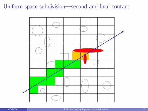
Uniform space subdivision—second and final contact

COSC342 Efficient ray tracing—spatial subdivision 20

Why is this scene bad for uniform space subdivision?

COSC342 Efficient ray tracing—spatial subdivision 21

Adaptive Subdivision

I Instead of lots of little empty cells, let’s aim to make the empty cellsas big as possible.

I Use a tree structure to create a hierarchy of bounding cubes.

I You will get fewer voxels.

I Is there a down side?

I Related approaches: Octrees/BSP-trees/kd-trees

COSC342 Efficient ray tracing—spatial subdivision 22

Quadtrees—subdivision order: cyan, green, blue, red

COSC342 Efficient ray tracing—spatial subdivision 23

Octrees—applying the Quadtree concept in 3D

I Divide until a cell has one object in it, or is too small.

I Octrees facilitate raytracing CSG objects well (we will cover CSG in alater lecture).

I . . . but the voxel-stepping algorithm is no longer obvious.

I (For historical contests between uniform and non-uniform spatialsubdivision over the years, see the “Ray Tracing News” archives)

COSC342 Efficient ray tracing—spatial subdivision 24

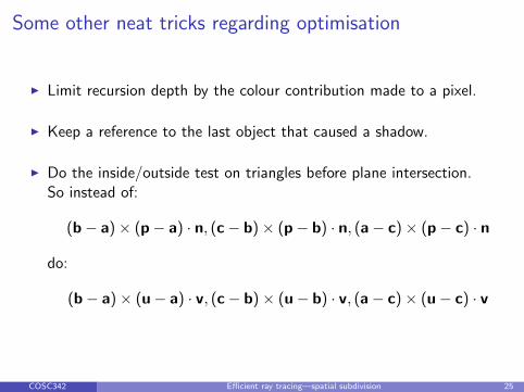
Some other neat tricks regarding optimisation

I Limit recursion depth by the colour contribution made to a pixel.

I Keep a reference to the last object that caused a shadow.

I Do the inside/outside test on triangles before plane intersection.So instead of:

(b− a)× (p− a) · n, (c− b)× (p− b) · n, (a− c)× (p− c) · n

do:

(b− a)× (u− a) · v, (c− b)× (u− b) · v, (a− c)× (u− c) · v

COSC342 Efficient ray tracing—spatial subdivision 25