Correlations and clustering in the trading of members

of the London Stock Exchange

Ilija I. ZovkoCenter for Nonlinear Dynamics in Economics and Finance,

University of Amsterdam, The Netherlands∗†

Santa Fe Institute, 1399 Hyde Park Road, Santa Fe, NM 87501, USA andRiskData, 6 rue d’Amiral Coligny, 75001 Paris, France

J. Doyne FarmerSanta Fe Institute, 1399 Hyde Park Road, Santa Fe, NM 87501, USA

This paper analyzes correlations in patterns of trading of different members ofthe London Stock Exchange. The collection of strategies associated with a memberinstitution is defined by the sequence of signs of net volume traded by that insti-tution in hour intervals. Using several methods we show that there are significantand persistent correlations between institutions. In addition, the correlations arestructured into correlated and anti-correlated groups. Clustering techniques usingthe correlations as a distance metric reveal a meaningful clustering structure withtwo groups of institutions trading in opposite directions.

Contents

I. Introduction 1

A. The LSE dataset 2

B. Measuring correlations betweenstrategies 2

II. Significance and structure in thecorrelation matrices 3

A. Density of the correlation matrixeigenvalue distribution 4

B. Bootstrapping the largesteigenvalues 6

C. Clustering of trading behaviour 8

D. Time persistence of correlations 11

III. Conclusions 13

∗This work was funded by Barclays Bank and Na-tional Science Foundation grant 0624351. Any opin-ions, findings, and conclusions or recommendationsexpressed in this material are those of the authorsand do not necessarily reflect the views of the Na-tional Science Foundation.†Electronic address: zovko@santafe.edu

References 14

I. INTRODUCTION

The aim of this paper is to examine theheterogeneity of the trading strategies asso-ciated with different members of the LondonStock Exchange (LSE). This is made possi-ble by a dataset that includes codes identi-fying which member of the exchange placedeach order. While we don’t know who themember actually is, we can link together thetrading orders placed by the same member.Member firms can be large investment banks,in which case the order-flow associated withthe code will be an aggregation of variousstrategies used by the bank and its clients,or at the other extreme it can be a singlehedge fund. Thus, while we cannot iden-tify patterns of trading at the level of indi-vidual trading strategies, we can test to seewhether there is heterogeneity in the collec-tions of strategies associated with differentmembers of the exchange. For conveniencewe will refer to the collection of strategies

2

associated with a given member of the ex-change as simply a strategy and the memberof the exchange as simply an institution, butit should be borne in mind throughout that“a strategy” is typically a collection of strate-gies, which may reflect the actions of severaldifferent institutions, and thus may internallybe quite heterogeneous.

We define a strategy by its actions, i.e. bythe net trading of an institution as a functionof time. If the net volume traded by an insti-tution in a period of time is positive there isan net imbalance of buying, and conversely,if the net volume is negative there is a netimbalance of selling. We test to see whethertwo strategies are similar in terms of theircorrelations in the times when they are netbuyers and when they are net sellers.

Two studies similar in spirit to this oneare [5, 11] in which the authors analyse trad-ing strategies using data from the SpanishStock Exchange. A number of related studiesanalysing market correlations can be foundin [2–4, 6–10].

A. The LSE dataset

The LSE is a hybrid market with two trad-ing mechanisms operating in parallel. Oneis called the on-book or “downstairs” mar-ket and operates as an anonymous electronicorder book employing the standard continu-ous double auction. The other is called theoff-book or “upstairs” market and is a bilat-eral exchange where trades are arranged viatelephone. We analyse the two markets sep-arately.

The market is open from 8:00 to 16:30,but for this analysis we discarded data fromthe first hour (8:00 – 9:00) and last half hourof trading (16:00 – 16:30) in order to avoidpossible opening and closing effects.

We base the analysis on four stocks, Voda-fone Group (VOD, telecomunications), As-traZeneca (AZN, pharmaceuticals), LloydsTSB (LLOY, insurance) and Anglo American(AAL, mining). We chose VOD as it is one

of the most liquid stocks on the LSE. LLOYand AZN are examples of frequently tradedliquid stocks, and AAL is a low volume illiq-uid stock.

B. Measuring correlations betweenstrategies

The institution codes we use in this anal-ysis are re-scrambled by the exchange eachmonth for privacy reasons1. This naturallydivides the dataset into monthly intervalswhich we treat as independent samples. Thedata spans from September 1998 to May2001, so we have 32 samples for each stock.

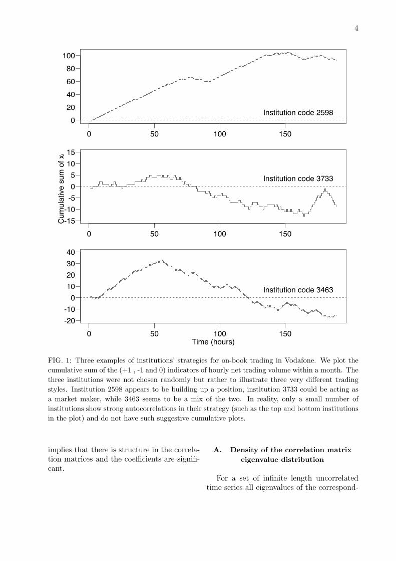
In order to define the trading strategieswe further divide the monthly samples intohourly intervals. We believe that one houris a reasonable choice, capturing short timescale intraday variations, but also providingsome averaging to reduce noise. For each ofthese hour intervals and for each institutionindividually, we calculate the net traded vol-ume in monetary units (British Pounds). Netvolume is total buy volume minus total sellvolume. We then assign to each institutionand hour interval a +1, -1 or 0 describing it’sstrategy in that interval. If the net volumein an interval is positive (the institution inthat period is a net buyer) we assign it thevalue +1. If the institution’s net volume inthe interval is negative (the institution is anet seller) we assign it the value -1. If the in-stitution is not active within the interval weassign it the value 0. We discard institutionsthat are not active for more than 1/3 of thetime.

Three examples of trading strategies areshown in figure 1. The examples show cumu-lated trading strategies for three institutions

1 However, we have found a way to track institu-tions’ trading on the on-book market for longertime periods. We use this fact in a subsequentpart of the paper. More about this later in thetext.

3

trading Vodafone on-book in the month ofNovember 2000.

In the end we obtain for each monthof trading a set of time series representingthe net trading direction for each institutionxi(t), which can be organized in a ’strategymatrix’ M with dimensions N × T , whereN is the number of active institutions andT is the number of hour intervals in thatmonth. The number of active institutionsvaries monthly and between stocks. Typicalvalue of N for the on-book market for liquidstocks is around N ∼ 70, and for less liq-uid stocks N ∼ 40. For the off-book market,the numbers are 1.5 to 2 times larger. Thenumber of hourly intervals depends on thenumber of working days in a month, and isaround T = 7× 20 = 140.

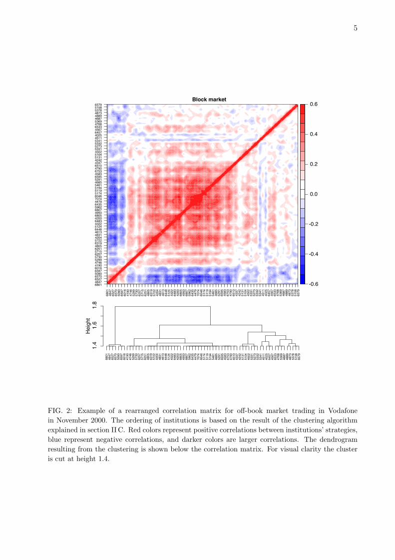
Given the monthly strategy matrices Mwe then construct the N × N monthly cor-relation2 matrices between the institutions’strategies. A color example of a correlationmatrix for off-book trading in Vodafone inNovember 2000 is given in the top panel offigure 2. Dark colors represent high abso-lute correlations, with red positive and bluenegative. Since the ordering of institutionsis arbitrary we use the ordering suggested bya clustering algorithm as explained later inthe text. It is visually suggestive that thecorrelations are not random: Some groups ofinstitutions are strongly anticorrelated withthe rest while in turn being positively corre-lated among themselves.

A formal test of significance involving thet-test cannot be used as it assumes normallydistributed disturbances, whereas we havediscrete ternary values. Later in the text weuse a bootstrap approach to test the signifi-cance. Now, however, we test the significanceof the correlation coefficients using a stan-dard algorithm as in ref. [1]. The algorithmcalculates the approximate tail probabilities

2 Since the data assumes only three distinct values(0,1 and -1) Pearson and Spearman correlationsare equivalent.

for Spearman’s correlation coefficient ρ. Itsprecision unfortunately degrades when thereare ties in the data, which is the case here.With this caveat in mind, as a preliminarytest, we find that, for example, for on-booktrading in Vodafone for the month of May2000, 10.3% of all correlation coefficients aresignificant at the 5% level. Averaging over allstocks and months, the average percentage ofsignificant coefficients for on-book trading is10.5% ± 0.4%, while for off-book trading itis 20.7% ± 1.7%. Both of these averages aresubstantially higher than the 5% we wouldexpect randomly with a 5% acceptance levelof the test.

II. SIGNIFICANCE ANDSTRUCTURE IN THE CORRELATION

MATRICES

The preliminary result of the previous sec-tion that some correlation coefficients arenon-random is further corroborated by test-ing for non-random structure in the correla-tion matrices. The hypothesis that there isstructure in the correlation matrices containsthe weaker hypothesis that some coefficientsare statistically significant.

The test for structure in the matriceswould involve multiple joint tests for the sig-nificance of the coefficients. An alternativemethod, however, is to examine the eigen-value spectrum of the correlation matrices.Intuitively, one can understand the relationbetween the two tests by remembering thateigenvalues λ are roots of the characteristicequation det(A−λ1) = 0, and that the deter-minant is a sum of permutations of productsof the matrix elements det(A) =

∑π επΠπaπ,

where π are the permutations and επ is theLevi-Civita antisymmetric tensor. On theother hand the test is directly related to prin-cipal component analysis, as the eigenvaluesof the correlation matrix determine the prin-cipal components.

The existence of empirical eigenvalueslarger than the values expected from the null

4

0 50 100 150

020406080

100

Institution code 2598

0 50 100 150-15-10

-505

1015

Cum

ulat

ive

sum

of x

i

Institution code 3733

0 50 100 150-20-10

010203040

Time (hours)

Institution code 3463

FIG. 1: Three examples of institutions’ strategies for on-book trading in Vodafone. We plot thecumulative sum of the (+1 , -1 and 0) indicators of hourly net trading volume within a month. Thethree institutions were not chosen randomly but rather to illustrate three very different tradingstyles. Institution 2598 appears to be building up a position, institution 3733 could be acting asa market maker, while 3463 seems to be a mix of the two. In reality, only a small number ofinstitutions show strong autocorrelations in their strategy (such as the top and bottom institutionsin the plot) and do not have such suggestive cumulative plots.

implies that there is structure in the correla-tion matrices and the coefficients are signifi-cant.

A. Density of the correlation matrixeigenvalue distribution

For a set of infinite length uncorrelatedtime series all eigenvalues of the correspond-

5

-0.6

-0.4

-0.2

0.0

0.2

0.4

0.66801

4847

6527

6570

5090

6597

6016

4190

4746

5299

5730

6257

5715

6251

4805

6319

5722

4204

4831

4613

6448

5124

4322

6483

4200

6805

4950

6807

5962

6435

4479

7074

6046

5174

5119

5194

5461

4685

5291

6595

4583

6753

4790

6510

4337

4242

5131

5104

4502

5331

5273

5332

5341

4511

4025

6457

4567

6533

4768

5369

4687

4889

4873

5378

5158

6579

680148476527657050906597601641904746529957306257571562514805631957224204483146136448512443226483420068054950680759626435447970746046517451195194546146855291659545836753479065104337424251315104450253315273533253414511402564574567653347685369468748894873537851586579

Block market6801

4847

6527

6570

5090

6597

6016

4190

4746

5299

5730

6257

5715

6251

4805

6319

5722

4204

4831

4613

6448

5124

4322

6483

4200

6805

4950

6807

5962

6435

4479

7074

6046

5174

5119

5194

5461

4685

5291

6595

4583

6753

4790

6510

4337

4242

5131

5104

4502

5331

5273

5332

5341

4511

4025

6457

4567

6533

4768

5369

4687

4889

4873

5378

5158

6579

1.4

1.6

1.8

Heig

ht

FIG. 2: Example of a rearranged correlation matrix for off-book market trading in Vodafonein November 2000. The ordering of institutions is based on the result of the clustering algorithmexplained in section II C. Red colors represent positive correlations between institutions’ strategies,blue represent negative correlations, and darker colors are larger correlations. The dendrogramresulting from the clustering is shown below the correlation matrix. For visual clarity the clusteris cut at height 1.4.

6

ing correlation matrix (which in this casewould be diagonal) are equal to 1. For finitelength time series, however, even if the un-derlying generating processes are completelyuncorrelated, the eigenvalues will not exactlybe equal to one - there will be some scatteraround one. This scattering is described by aresult from random matrix theory [3, 4, 10].For N random uncorrelated variables, each oflength T , in the limit T → ∞ and N → ∞while keeping the ratio Q = T/N ≥ 1 fixed,the density of eigenvalues p(λ) of the corre-lation matrix is given by the functional form

p(λ) =Q

2πσ2

√(λmax − λ)(λ− λmin)

λ

λmaxmin = σ2(1 + 1/Q± 2√

1/Q). (1)

σ2 is the variance of the time series andλ ∈ [λmin, λmax]. Apart from being a limitingresult, this expression is derived for Gaussianseries. As it turns out the Gaussian assump-tion is not critical, at least not for the rightlimit λmax, which is the one of interest forthis study. We show in a subsequent sectiona simulation result confirming this observa-tion.

A further consideration is the fact that theparameters Q = T/N and σ change everymonth3, as both the number of hour intervalsand the number of institutions vary. Conse-quently the predicted eigenvalue density un-der the null changes from month to month. Inprinciple we should construct a separate testfor each month, comparing the eigenvalues ofa particular month with the null distributionusing the appropriate value of Q = T/N andσ. However, monthlyQ and σ do not vary toomuch, and the variation does not change thefunctional form of the null hypothesis sub-stantially. In view of the fact that Eq. 1 isvalid only in the limit in any case, we pooleigenvalues for all months together, construct

3 σ is calculated mechanically using the standard for-mula, as if the time series had a continuous densityfunction rather than discrete ternary values.

a density estimate and compare it with thenull using the monthly averages of Q and σ.

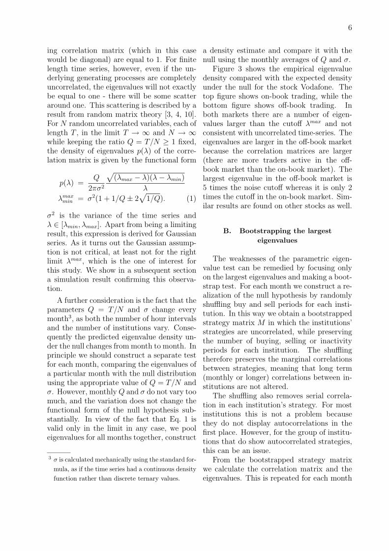
Figure 3 shows the empirical eigenvaluedensity compared with the expected densityunder the null for the stock Vodafone. Thetop figure shows on-book trading, while thebottom figure shows off-book trading. Inboth markets there are a number of eigen-values larger than the cutoff λmax and notconsistent with uncorrelated time-series. Theeigenvalues are larger in the off-book marketbecause the correlation matrices are larger(there are more traders active in the off-book market than the on-book market). Thelargest eigenvalue in the off-book market is5 times the noise cutoff whereas it is only 2times the cutoff in the on-book market. Sim-ilar results are found on other stocks as well.

B. Bootstrapping the largesteigenvalues

The weaknesses of the parametric eigen-value test can be remedied by focusing onlyon the largest eigenvalues and making a boot-strap test. For each month we construct a re-alization of the null hypothesis by randomlyshuffling buy and sell periods for each insti-tution. In this way we obtain a bootstrappedstrategy matrix M in which the institutions’strategies are uncorrelated, while preservingthe number of buying, selling or inactivityperiods for each institution. The shufflingtherefore preserves the marginal correlationsbetween strategies, meaning that long term(monthly or longer) correlations between in-stitutions are not altered.

The shuffling also removes serial correla-tion in each institution’s strategy. For mostinstitutions this is not a problem becausethey do not display autocorrelations in thefirst place. However, for the group of institu-tions that do show autocorrelated strategies,this can be an issue.

From the bootstrapped strategy matrixwe calculate the correlation matrix and theeigenvalues. This is repeated for each month

7

0 1 2 3 4 5

0.001

0.005

0.010

0.050

0.100

0.500

1.000

Lo

g d

en

sity

VOD, Limit order book

0 5 10 15

0.001

0.005

0.010

0.050

0.100

0.500

1.000

Eigenvalues of the correlation matrix

Lo

g d

en

sity

VOD, Block market

FIG. 3: Empirical density of eigenvalues of the correlation matrices (red) compared to the theo-retical density for a random matrix (blue). We see that there are many eigenvalues not consistentwith the hypothesis of a random matrix.

separately 1000 times.

As already noted, instead of looking atthe significance of all empirical eigenvalues,we focus only on the largest two eigenvaluesfor each month. Correspondingly, we com-pare them with the null distribution of the

two largest eigenvalues for each month: Fromeach of the 1000 simulated correlation matri-ces, we keep only the largest two. We aretherefore comparing the empirical largest twoeigenvalues with an ensemble of largest eigen-values from the 1000 simulated correlation

8

matrices that correspond to the null appro-priate to that month. In this way the vari-ations of Q and σ, as well as small sampleproperties, are taken into account in the test.

Figure 4 shows the results for all 32months of trading in Vodafone. Again, thetop figure shows the monthly eigenvalues forthe on-book market while the bottom figurefor the off-book market. The largest empir-ical monthly eigenvalues are shown as bluepoints. They are to be compared with theblue vertical error bars which represent thewidth of the distribution of the maximumeigenvalues under the null. The error barsare centered at the median and represent twostandard deviations of the underlying distri-bution. Since the distribution is relativelyclose to a normal, the width represents about96% of the density mass. The analogousred symbols show the second largest eigen-value for each month. We first note that themedian of the distribution of the maximumeigenvalue under the random null fluctuatesroughly between 2.4 and 2.5. These valuesare not so different from λmax = 2.5 whichwe used in the parametric test. It even seemsthat in small samples and with ternary data,the tendency of λmax is to decline as the num-ber of points used decreases, further strength-ening the parametric test. The same conclu-sion can be drawn by looking at the off-bookmarket.

The largest eigenvalue is significant in allmonths on both markets. Corroborating theparametric test, the largest eigenvalues onthe off-book market are relatively furtheraway from the corresponding null than forthe on-book market, confirming the observa-tion that the correlations are stronger for off-book trading. However, being stronger, theyare perhaps of a more simple nature: Thesecond largest eigenvalue is almost never sig-nificant for off-book trading, while on the on-book market it is quite often significant.

C. Clustering of trading behaviour

The existence of significant eigenvalues al-lows us to use the correlation matrix as adistance measure in the attempt to classifyinstitutions into groups of similar or dis-similar trading patterns. We apply clus-tering techniques using a metric chosen sothat two strongly correlated institutions are’close’ and anti-correlated institutions are ’faraway’. A functional form fulfilling this re-quirement and satisfying the properties of be-ing a metric is [2]

di,j =√

2 · (1− ρi,j), (2)

where ρi,j is the correlation coefficient be-tween strategies i and j. We have tried sev-eral reasonable modifications to this form butwithout obvious differences in the results. Ul-timately the choice of this metric is influencedby the fact that it has been successfully usedin other studies [2]. We use complete linkageclustering, in which the distance between twoclusters is calculated as the maximum dis-tance between its members. We also tried us-ing minimum distance (called “single linkageclustering”), which produced clusters similarto minimal spanning trees but without obvi-ous benefits4.

The first benefit of creating a clusteringis to rearrange the columns of the corre-lation matrix according to cluster member-ship. In the top part of figure 2 we alreadyshowed the rearranged correlation matrix foroff-book trading in Vodafone for May 2000.In the bottom part is the corresponding den-drogram. In the correlation matrix one no-tices a highly correlated large group of insti-tutions as the red block of the matrix. Onealso notices a smaller number of institutionswith strategies that are anti-correlated with

4 We have also constructed minimal spanning treesfrom the data but without an obvious interpreta-tion.

9

Nth

larg

est e

igen

valu

e

●

●

●

●

●●

●

●

●

●

●

●

●

●●

●

●

●

●

●

●

●●

●

●

●

●

●

●

●

●

●

●●

● ●

●

●●

●●

●●

●

●

●●

●

●

● ● ●

●

●

● ●

●

●

●

●

●●

●

●

1 5 10 15 20 25 30

2.0

2.5

3.0

3.5

4.0

4.55.0

Month

Nth

larg

est e

igen

valu

e ● ●●

●

●

●●

●●

●

●

●

●

●

●

●

●

●

●●

●●

●

●

●

●

●

●

●

●●

●●

● ●

●

●

●

●● ●

●

● ●●

●

● ●

●

●

●● ●

●● ●

● ●●

●

● ●●

●

1 5 10 15 20 25 30

2

4

6

810121416

●

●

Largest empirical eigenvalueLargest null model eigenvalue2nd largest empirical eigenvalue2nd largest null model eigenvalue

FIG. 4: Largest eigenvalues of the correlation matrix over the 32 months for the stock Vodafone.The top figure is for on-book trading, the bottom for off-book trading. Blue points represent thelargest empirical eigenvalues and are to be compared with the blue error bars which denote the nullhypothesis of no correlation. Red points are the second largest eigenvalues and are to be comparedwith the red error bars. The error bars are centered at the median and and correspond to twostandard deviations of the distribution of largest monthly eigenvalues under the null

the large group. These institutions in turnare correlated among themselves. Finally, tothe right part of the matrix there is a groupof institutions that is weakly correlated withboth of the previous two. These basic obser-vations are also confirmed in the clusteringdendrogram - the dendrogram is plotted so

that the institutions in the correlation matrixcorrespond to the institutions in the dendro-gram. Cutting the dendrogram at height 1.7for example, we recover the two main clustersconsisting of the correlated red and the anti-correlated blue institutions. Cutting the den-drogram at a finer level, say just below 1.6,

10

-0.6

-0.4

-0.2

0.0

0.2

0.4

0.6

353342

351546

283265

282040

352318

282782

350894

352862

281876

352658

350770

352086

353741

302688

281720

283454

311776

351618

323265

321190

353546

341759

352990

282548

282598

341110

353794

351793

351814

352654

351432

311472

282533

352065

353062

321739

353315

282575

351835

282534

321522

353117

353342351546283265282040352318282782350894352862281876352658350770352086353741302688281720283454311776351618323265321190353546341759352990282548282598341110353794351793351814352654351432311472282533352065353062321739353315282575351835282534321522353117

Limit order market

1.40

1.50

1.60

Height

353342

351546

283265

282040

352318

282782

350894

352862

281876

352658

350770

352086

353741

302688

281720

283454

311776

351618

323265

321190

353546

341759

352990

282548

282598

341110

353794

351793

351814

352654

351432

311472

282533

352065

353062

321739

353315

282575

351835

282534

321522

353117

FIG. 5: Correlation matrix and the clustering dendrograms for on-book trading in VOD in Novem-ber 2000. The correlated and anti-correlated groups of institutions are easily identifiable, however,for this month, the clustering algorithm does not properly classify the institutions at the top clus-tering level. We have added lines to help guide the eye to perhaps a better clustering than thealgorithm came up with. It seems that the leftmost group of correlated institutions should havebeen clustered together with the rest of the correlated institutions.

we also recover the weakly correlated clusterof institutions. The structure of the dendro-gram below 1.4 is suppressed for clarity ofthe figure, as those levels of detail are noisy.For other months and other stocks we ob-serve very similar patterns. The top cluster-ing level typically will classify institutions asa larger correlated group and a smaller anti-

correlated group.

The clustering for the on-book market issimilar, though weaker. Figure 5 shows thecorrelation matrix and the clustering dendro-gram for the on-book trading for the samemonth and stock as the example we showedearlier in figure 2. We again see corre-lated and anti-correlated groups of institu-

11

tions, as well as the weakly correlated group.The clustering algorithm in this case, how-ever, does not select the correlated and anti-correlated groups at the top level of the clus-tering, selecting rather the weakly correlatedgroup in one cluster and the other two in theother. At a finer level of clustering (lowerheight in the dendrogram) the three groupsare clustered separately. The clustering algo-rithm and the distance metric we currentlyuse may not be optimal in selecting the insti-tutions into clusters, but there is indicationthat the clustering makes sense. In any case,the existence of clusters of institutions basedon the correlation in their strategies suggeststhat it may be possible to develop a taxon-omy of trading strategies.

D. Time persistence of correlations

Time persistence, when it is possible to in-vestigate it, offers a fairly robust and strongtest for spuriousness. If a correlation is spu-rious it is not likely to persist in time. Incontrast, if the correlations are persistentthan the clusters of institutions also persistin time. As noted before, the LSE rescram-bles the codes assigned to the institutions atthe turn of each month. It is therefore notpossible to simply track the correlations be-tween institutions in time. Fortunately, thereis a partial solution to this problem. By ex-ploiting other information in the dataset weare able to unscramble the codes over a fewmonths in a row for some institutions. Unfor-tunately, the method works only for tradingon the on-book market and typically does notwork for institutions that do not trade fre-quently5. Therefore, the results reported in

5 In the LSE data we use each order submitted tothe limit order book is assigned a unique identi-fier. This identifier allows us to track an order inthe book and all that happens to it during its his-tory. If at the turn of the month (the scramblingperiod) an institution has an order sitting in the

this section concern only the on-book marketand are based mostly on more active insti-tutions. Since the correlations are typicallystronger in the off-book market, we believethe results shown here would hold also forthe off-book market, and perhaps be evenstronger.

Given the problems with tracking institu-tions in time we focus only on persistence upto two months. To form a dataset we seek allpairs of institution codes that are present atthe market for two months in a row. For allsuch pairs we compare the correlation in thefirst of the two months c1 to the correlation inthe second of the two months c2. If the cor-relation between two institutions was high inthe first month, we estimate how likely is itthat it will be high in the second month aswell by calibrating a simple linear regression

c2 = α + β · c1 + ε, (3)

assuming ε to be i.i.d. Gaussian. For thestock VOD we identify 7246 linkable consec-utive pairs, for AZN 1623, for LLOY 1930and for AAL 640. All the regressions are wellspecified - the residuals are roughly normaland i.i.d. The regression results for the on-book market are summarized in table I. Allstocks show significant and positive slope co-efficients with R2 around 5%. Correlated in-stitutions tend to stay correlated, though therelationship is not strong.

book, we can connect the institution codes asso-ciated with the order before and after the scram-bling. For example, if an order coded AT82F31E13was submitted to the book on the 31st by institu-tion 2331, and that same order was then canceledon the 1st by institution 4142, we know that the in-stitution that was 2331 was recoded as 4142. Thistypically allows us to link the codes for most ac-tive institutions for many months in a row, and inseveral cases even for the entire 32 month period.The LSE has indicated that they do not mind usdoing this, and has since provided us with the in-formation we need to unscramble all the codes.

12

TABLE I: Regression results of equation 3 for correlations between institutions for two consecutivemonths. Significant slope coefficients show that if two institutions’ strategies were correlated inone month, they are likely to be correlated in the next one as well. The table does not containthe off-book market because we cannot reconstruct institution codes for the off-book market in thesame way as we can for the on-book market. The ± values are the standard error of the coefficientestimate and the values in the parenthesis are the standard p-values.

On-book market

Stock Intercept Slope R2

AAL -0.010 ± 0.004 (0.02) 0.25 ± 0.04 (0.00) 0.061

AZN -0.01 ± 0.003 (0.00) 0.14 ± 0.03 (0.00) 0.019

LLOY 0.003 ± 0.003 (0.28) 0.23 ± 0.02 (0.00) 0.053

VOD 0.008 ± 0.001 (0.00) 0.17 ± 0.01 (0.00) 0.029

Another sign of persistence is if an insti-tution gets consistently clustered in a givencluster. If two institutions tend to be clus-tered in a given cluster more often than ran-dom then we can infer that the cluster ismeaningful. For this purpose we must have away to distinguish the clusters by some prop-erty. A visual examination of many correla-tion matrices and dendrograms makes it clearthat it is often the case that the two top levelclusters are typically of quite different sizes.It seems natural to call them the majorityand the minority cluster. Even though it wasnot always the case, the number of membersin the two top clusters differed by a largenumber more often than not. Acknowledg-ing that this may not be a very robust dis-tinguishing feature, we choose it as a simplemeans to distinguish the main clusters.

The probability that an institution wouldrandomly be clustered in the minority a givennumber of times is analogous to throwing abiased coin the same number of times, withthe bias being proportional to the ratio ofthe sizes of the two clusters. If the probabil-ity for being in the minority was a constantp throughout the K months, the expectednumber of times x an institution would ran-domly end up in the minority would be de-

scribed by a binomial distribution

B(x, p,K) =

(x

K

)px(1− p)k−x. (4)

In our case, however, the probability of beingin the minority is not a constant, but variesmonthly with the number of active institu-tions and the size of the minority. If thesize of the minority is half the total numberof institutions, the probability of ending inthe minority by chance is 1/2. If the size ofthe minority is very small compared to thenumber of total institutions, the probabilityof ending in that cluster by chance is conse-quently very small. Denoting by νk the num-ber of active institutions in month k and byµk the number of institutions in the minoritycluster, then the probability for an institu-tion to be in minority for month k by chanceis pk = µk/νk. The expected number of timesfor an institution to be in the minority bychance is then

P (x, pk, K) =∏

k∈min

pk ·∏

k∈maj

(1− pk), (5)

where k indexes the months in which theinstitution was in the majority or minority.A further complication is that not all insti-tutions are active on the same months, sothat the probability density differs from in-stitution to institution: Depending on which

13

months the institution was active, the aboveproduct picks out the corresponding proba-bilities pk. Because of this complication wecalculate the probability density for each in-stitution through a simulation. We simplypick out the months the institution was ac-tive, for each month draw a trial randomlyaccording to pk, and calculate the number oftimes the trial was successful, i.e., that the in-stitution ended up in the minority. Repeatingthis many times we get the full distributionfunction for the number of times the institu-tion can end up in the minority at randomfor each institution.

TABLE II: Result of the test on minority mem-bers for on-book trading in Vodafone. In boldare institutions whose behavior is not consistentwith the hypothesis of random behavior.

Inst. Times in Out of Prob. of non-code minority possible -random behavior

3265 16 32 0.99

2548 7 32 0.14

2575 6 32 0.07

2533 3 19 0.11

2040 14 31 0.97

1720 9 20 0.93

1876 5 14 0.73

2688 8 30 0.34

1776 11 22 0.99

2086 9 23 0.86

0867 10 22 0.95

2995 12 20 1.00

2569 7 21 0.64

Similarly, because we are using the insti-tution codes over intervals of more than onemonth, we can perform this test only for insti-tutions on the on-book market. We limit thetest to the stock Vodafone and apply it onlyon institutions that we can track for morethan 12 out of the 32 months. This resultsin 13 institutions on which we base the test.For other stocks we are not able to track in-

stitutions for long periods and the power ofthe test would be weak.

The results for the 13 institutions aregiven in table II. The leftmost column isthe institution code, followed by the numberof times that institution has been in the mi-nority. The column named ’Out of possible’counts the number of months an institutionhas been present in the market - it is the max-imum number of times it could have been inthe minority. Finally, the rightmost columngives one minus the probability that the in-stitution could have randomly been so manytimes in the minority. We choose to displayone minus the probability as it represents theprobability of accepting the hypothesis thatthe behavior of that institution is not consis-tent with the random null hypothesis. Mostinstitutions have quite high probabilities ofnon-random behavior and in bold we selectthe institutions which pass the test at the5% level. Out of 13 institutions, 5 of themhave been in the minority cluster more oftenthan they would have been just by chance atthe 5% acceptance level. This is substantiallyhigher than the expected number of 0.65 outof 13 tested at this acceptance level.

III. CONCLUSIONS

We have shown that even very crude def-initions of institutions’ strategies defined onintervals of an hour period produce signifi-cant and persistent correlations. On the off-book market these correlations are organizedin a way that there is typically a small groupof institutions anti-correlated with a largersecond group. The strategies within the twogroups are correlated. Clustering analysisalso clearly reveals this structure. The vol-ume transacted by the smaller group, typi-cally containing no more than 15 institutionson Vodafone, accounts for about half of thetotal trading volume. The larger group, typ-ically of around 80 institutions on Vodafone,transacts the remaining half of the total tradevolume. This is an indication that the smaller

14

group can be identified as the group of deal-ers on the off-book market. They provide liq-uidity for the larger group of institutions andtheir strategies are anti-correlated: the deal-ers buy when the other institutions are sell-ing and vice versa. The single large monthlyeigenvalue in the off-book market is relatedto this basic dynamics.

Contrary to the off-book market, the on-book market does not display only one largeeigenvalue. There are typically one or twosignificant eigenvalues for each month. Theeigenvalues are relatively smaller and thecorrelations not as strong. Still, we areable to identify the basic clustering structureseen on the off-book market, namely a smalland large group of anti-correlated strategies.However, the volume traded by the smallcluster does not seem to equal the volumeof the large cluster. The dynamics seems tobe more complicated. The largest eigenvaluemay still be related to transactions betweenthe two clusters of institutions, however theoccasional second largest eigenvalue suggests

that there is more complicated dynamics tak-ing place.

These results suggest that trading on theLSE is a relatively structured process in theaspect of trading strategies. At a given time,there are groups of institutions all trading inthe same direction, with other groups tradingin the opposite direction, providing liquidity.

It is important to stress that what we haveconveniently labeled a “strategy” is more typ-ically a collection of strategies all being exe-cuted by the same member of the exchange.From this point of view it is particularly re-markable that we observe heterogeneity, asit depends on the tendency of certain typesof strategies to execute through particularmembers of the exchange (or in some casesthat pure strategies take the expense to pur-chase their own membership). One expectsthat if we were able to observe actual accountlevel information we would see much cleanerand stronger similarities and differences be-tween strategies.

[1] Best, D. J. and Roberts, D. E. (1975). Algo-rithm as 89: The upper tail probabilities ofspearman’s rho. Journal of Applied Statis-tics, 24:377–379.

[2] Bonanno, G., Vandewalle, N., and Man-tegna, R. N. (2000). Taxonomy of stockmarket indices. Phys. Rev. E, 62(6):R7615–R7618.

[3] Laloux, L., Cizeau, P., Bouchaud, J.-P., andPotters, M. (1999a). Noise dressing of finan-cial correlation matrices. Phys. Rev. Lett.,83(7):1467–1470.

[4] Laloux, L., Cizeau, P., Potters, M., andBouchaud, J.-P. (1999b). Random matrixtheory and financial correlations. Workingpaper, Science and Finance Capital FundManagement.

[5] Lillo, F., Esteban, M., Vaglica, G., andMantegna, R. N. (2007). Specialization ofstrategies and herding behavior of trading

firms in a financial market. ArXiv e-prints,(ArXiv:0707.0385).

[6] Mantegna, R. N. (1999). Information andhierarchical structure in financial markets.Computer Physics Communications, 121-122:153–156.

[7] Onnela, J.-P., Chakraborti, A., Kaski, K.,Kertesz, J., and Kanto, A. (2003). Dy-namics of market correlations: Taxonomyand portfolio analysis. Physical ReviewE (Statistical, Nonlinear, and Soft MatterPhysics), 68(5):056110.

[8] Plerou, V., Gopikrishnan, P., Rosenow, B.,Amaral, L. A. N., Guhr, T., and Stanley,H. E. (2002). Random matrix approach tocross correlations in financial data. Phys.Rev. E, 65(6):066126.

[9] Plerou, V., Gopikrishnan, P., Rosenow, B.,Nunes Amaral, L. A., and Stanley, H. E.(1999). Universal and nonuniversal prop-

15

erties of cross correlations in financial timeseries. Phys. Rev. Lett., 83(7):1471–1474.

[10] Potters, M., Bouchaud, J.-P., and Laloux,L. (2005). Financial applications of randommatrix theory: Old laces and new pieces.Working paper, Science and Finance Capi-tal Fund Management.

[11] Vaglica, G., Lillo, F., Moro, E., and Man-tegna, R. N. (2007). Scaling laws ofstrategic behaviour and size heterogene-ity in agent dynamics. ArXiv e-prints,(arXiv:0704.2003v1).