The 14th IFToMM World Congress, Taipei, Taiwan, October 25-30, 2015 DOI Number: 10.6567/IFToMM.14TH.WC.OS13.055

Correlation of Singularity Analyses Based on Position and Velocity Kinematics

Soumyajit Roy∗ S. K. Saha † Sasanka Sekhar Sinha ‡

Indian Institute of Technology Kharagpur Indian Institute of Technology Delhi Indian Institute of Technology DelhiKharagpur, India New Delhi, India New Delhi, India

Abstract—Singularity analyses of manipulators are per-formed with great concern to avoid singular configurationsin which the driving motors and related hardware may facegreat difficulty to drive the manipulator joints further or themanipulator itself may become uncontrollable in certain re-gions. Position and velocity kinematics are common prac-tices for singularity analyses. Both the kinematics serve twodifferent purposes. Position kinematics directly proposesthe singularity manifold as well as the assembly configura-tions. On the other hand, velocity kinematics very easilyfinds a singular configuration. The present research pro-poses a unique procedure to correlate these two methods.Inverse kinematics in case of serial manipulators and for-ward kinematics for parallel manipulators act as a bridgebetween two different singularity analyses approaches. Thefact was established with relevant examples of 2-link 2-Rplanar serial manipulator, 3-link 3-R spatial serial manip-ulator and 4-bar linkage.

Keywords: Correlation, Position kinematics, Singularity analyses,Velocity kinematics.

I. IntroductionKinematics of manipulators has been a research field for

long time. It certainly becomes essential when singularityanalyses of manipulators are performed. Serial and paral-lel manipulators experience singularity, although, it is moreserious for parallel manipulators since they possess both“gain” and “loss” type singularities. Fortunately, serial ma-nipulators have only “loss” type singularities. In this typeof singularity, the manipulator loses one or more degrees offreedom (dof). However, in case of parallel manipulators,they gain extra degrees of freedom and become uncontrol-lable in the singular regions.

Singularity analyses can be performed from both positionand velocity kinematic point of view, as reported by severalresearchers. Generally, velocity kinematics gives differentsingular configurations of manipulators whereas, positionkinematics provides singularity manifold in the task space(a space where end-effector performs, which is defined bythe Cartesian coordinates) or configuration space (definedby joint coordinates of a manipulator) and of course the sin-gular configurations. There are numerous literatures avail-able in this regard. Only a few relevant ones are reported

∗soumyajit ju@yahoo.com†saha@mech.iitd.ac.in‡sasanka.sailesh@gmail.com

here. Williams et al. [1] proved Grashof’s law with polyno-mial discriminant. Wang et al. [2] described the singularityof serial manipulators based on screw theory. Merlet [3]and Gosselin et al. [4] analysed singular configuration ofclosed loop chains or parallel manipulators using velocityJacobian. Innocenti [5] also calculated the forward kine-matics of general Stewart Platform using polynomial form.Bandyopadhyay et al. [6] very elaborately discussed aboutthe velocity kinematics and subsequent configuration spacesingularities of different closed loop systems.

In this paper, a very unique finding has been reported.It is shown that inverse kinematic solution for serial ma-nipulators and forward kinematic solution for parallel ma-nipulators act as a bridge between singularity analyses us-ing position and velocity kinematics. They combined withthe velocity Jacobian approach invariably lead to the samesingularity manifold which normally comes out of positionkinematics.

The paper is organised as follows. Section II describesgeneral theory regarding position and velocity kinemat-ics and subsequently singularity analyses from those the-ories. Section III provides the correlation between themwith proper examples of serial and parallel manipulators.Finally Section IV concludes the findings of the current re-search and discusses few future scopes.

II. Generalised TheoryIn this section, the theories behind position and velocity

kinematics are presented in a generalised way. How singu-larity analyses are performed based on these theories is alsodescribed.

A. Position kinematicsPosition kinematics deals with the position of end effec-

tor of a manipulator for known values of joint coordinatesand vice-versa. In case of parallel manipulators, it is sub-jected to constrained equations also. A generalised kine-matic equation for position can be expressed as

η(q) = X (1)

where, η represents the system of equations, q denotes gen-eralised coordinates and X denotes the end-effector coor-dinate.

In forward kinematics all the joint coordinates, i.e., qare known. So, finding end-effector position, i.e., X isquite straight forward for serial manipulators. But, inverse

kinematics, i.e., to find joint coordinates for given end-effector position is fairly complex since Eqn. (1) is a setof non-linear trigonometric equations which can be solvedby proper elimination techniques using trigonometric iden-tities. Obviously, multiple solutions exist for a known end-effector position.

However, unlike serial manipulators forward kinemat-ics is not so straight forward in case of parallel manipula-tors because their kinematics is constrained by loop closureequations. Therefore, Eqn. (1) can be rewritten as

η(θ,φ) = 0 (2)

where, θ andφ are generalised coordinates representing ac-tuated joint variables and passive joint variables, respec-tively. Since, only θ is known for forward kinematicsEqn. (2) can be rewritten as

η(φ) = 0 (3)

Equation (3) can also be solved by proper elimination tech-nique. When inverse kinematics is performed for parallelmanipulators, only generalised coordinate corresponding toend-effector, φe are known. Closed loops are often brokendown to branches which are treated as serial chains to solvetheir inverse kinematics.

B. Velocity kinematicsLike position kinematics, velocity kinematics is also

a mapping between velocity of end-effector and rate ofchange of join coordinates with respect to time. To performvelocity kinematics of serial manipulators Eqn. (1) can bedifferentiated with respect to time to obtain [7]

v = [J(q)]q (4)

where, v is the velocity of the end-effector, q is the rate ofchange of joint variables and J(q) is the velocity Jacobian.However, for parallel manipulators, one needs to differen-tiate the loop closure constraint equation as expressed byEqn. (2) to get [6]

[K#(q)]θ + [K∗(q)]φ = 0 (5)

where,K#(q) andK∗(q) are the matrices whose columnsare partial derivatives of η(q) with respect to θ and φ, re-spectively. Therefore, φ can be obtained from Eqn. (5) as

φ = −[K∗(q)]−1[K#(q)]θ (6)

when, det[K∗(q)] 6= 0. To find end-effector velocity of aparallel manipulator, Eqn. (4) can be rewritten as [7]

v = [J#(q)]θ + [J∗(q)]φ (7)

where, J#(q) and J∗(q) are the matrices in whichcolumns are partial derivatives of J(q) with respect to θand φ, respectively. Replacing φ from Eqn. (6) in Eqn. (7)one can obtain

v = [Jeq(q)]θ (8)

where, Jeq(q) = J#(q)− [J∗(q)][K∗(q)]−1[K#(q)]

C. Singularity analysesSingularity analyses can be performed both from position

and velocity kinematics. The most important step of singu-larity analyses from position kinematics involves elimina-tions of variables from system of equations described byEqn. (1). There is no such established algorithm whichcan be universally applied to every system of equations.Choice of elimination method completely depends on thesystem of equation itself and to some extent on the experi-ence of the researchers. However, the aim of elimination isto reduce the number of variables, which eventually givesa polynomial equation in tangent function of a single jointvariable. The discriminant of this polynomial equation pro-vides information about singularity and singularity mani-fold. When the real roots of the polynomial equation mergetogether, discriminant vanishes and it signifies singularityof the manipulator. Repeated roots provide the singularconfiguration and, on the other hand, discriminant functionitself is the singularity manifold when equated to zero. Thedetails regarding this can be well understood in Section IIIwhen explained with examples.

Singularity analysis with velocity kinematics requiresanalysis of velocity Jacobian. It can be seen from Eqn. (4)that for some specific values of q, det[J(q)] is zero, i.e.,the Jacobian becomes singular and the serial manipulatoris said to be in singular configuration. Parallel manipu-lators also experience such singularity when det[Jeq(q)]in Eqn. (8) becomes zero. However, Eqn. (6) can onlybe written when det[K∗(q)] 6= 0. On the other hand, ifdet[K∗(q)] = 0 and θ is chosen to be zero, Eqn. (5) re-sults in a homogeneous equation [8]. Then Eqn. (5) yields[7]

[K∗(q)]φ = 0 (9)

Equation (9) represents an eigen-value problem and φ hasnon-trivial solutions. However, this type of singularity istermed as gain type of singularity which physically signifiesthat even if the actuated joints are locked, there are somespecific configurations of the manipulator in which the pas-sive joint variables will still have finite and real values, i.e.,the manipulator gains some extra degrees freedom.

III. Correlation between Singularity Analyses from Po-sition and Velocity Kinematics

As stated in Section I inverse and forward kinematic so-lutions were used to draw correlation between singularityanalyses based on position and velocity kinematics for se-rial and parallel manipulators, respectively. The example of2-link 2-R planar serial manipulator, 3-link 3-R spatial se-rial manipulator and 4-bar linkage are used to establish thefact. For all cases analytical methods were used only.

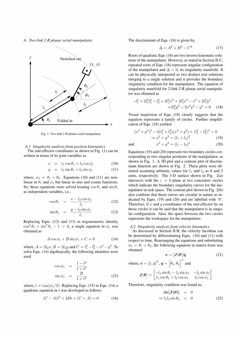
A. Two-link 2-R planar serial manipulator

Fig. 1: Two-link 2-R planar serial manipulator

A.1 Singularity analysis from position kinematicsThe end-effector coordinates as shown in Fig. (1) can be

written in terms of its joint variables as

x = l1 cos θ1 + l2 cosφ1 (10)y = l1 sin θ1 + l2 sinφ1 (11)

where, φ1 = θ1 + θ2. Equations (10) and (11) are non-linear in θ1 and φ1 but linear in sine and cosine functions.So, these equations were solved treating cos θ1 and sin θ1as independent variables, i.e.,

cos θ1 =x− l2 cosφ1

l1(12)

sin θ1 =y − l2 sinφ1

l1(13)

Replacing Eqns. (12) and (13) in trigonometric identitycos2 θ1 + sin2 θ1 − 1 = 0, a single equation in φ1 wasobtained as

A cosφ1 +B sinφ1 + C = 0 (14)

where, A = 2l2x, B = 2l2y and C = l21− l22−x2− y2. Tosolve Eqn. (14) algebraically, the following identities wereused

cosφ1 =1− t2

1 + t2

sinφ1 =2t

1 + t2(15)

where, t = tan(φ1/2). Replacing Eqn. (15) in Eqn. (14) aquadratic equation in t was developed as follows

(C −A)t2 + 2Bt+ (C +A) = 0 (16)

The discriminant of Eqn. (16) is given by,

∆ = A2 +B2 − C2 (17)

Roots of quadratic Eqn. (16) are two inverse kinematic solu-tions of the manipulator. However, as stated in Section II-C,repeated roots of Eqn. (16) represent singular configurationof the manipulator and ∆ = 0, its singularity manifold. Itcan be physically interpreted as two distinct real solutionsmerging to a single solution and it provides the boundarysingularity condition for the manipulator. The equation ofsingularity manifold for 2-link 2-R planar serial manipula-tor was obtained as

−l41 + 2l21l22 − l42 + 2l21x

2 + 2l22x2 − x4 + 2l21y

2

+2l22y2 − 2x2y2 − y4 = 0 (18)

Visual inspection of Eqn. (18) clearly suggests that theequation represents a family of circles. Further simplifi-cation of Eqn. (18) yielded

(x2 + y2)2 − 2(l21 + l22)(x2 + y2) + (l21 − l22)2 = 0

⇒ x2 + y2 = (l1 + l2)2 (19)

and x2 + y2 = (l1 − l2)2 (20)

Equations (19) and (20) represent two boundary circles cor-responding to two singular positions of the manipulator, asshown in Fig. 1. A 3D plot and a contour plot of discrim-inant function are shown in Fig. 2. These plots were ob-tained assuming arbitrary values for l1 and l2 as 6 and 2units, respectively. The 3-D surface shown in Fig. 2(a)intersects with the z = 0 plane at two concentric circleswhich indicate the boundary singularity curves for the ma-nipulator in task space. The contour plot shown in Fig. 2(b)also confirms that those curves are circular in nature as in-dicated by Eqns. (19) and (20) and are labelled with ‘0’.Therefore, if x and y coordinates of the end-effector lie onthose circles it can be said that the manipulator is in singu-lar configuration. Also, the space between the two circlesrepresents the workspace for the manipulator.

A.2 Singularity analysis from velocity kinematicsAs discussed in Section II-B, the velocity Jacobian can

be determined by differentiating Eqns. (10) and (11) withrespect to time. Rearranging the equations and substitutingφ1 = θ1 + θ2, the following equation in matrix-form wasobtained

v = [J(θ)]q (21)

where, v = [x, y]T , q =

[θ1, θ2

]Tand

J(θ) =

[−l1 sin θ1 − l2 sinφ1 −l2 sinφ1l1 cos θ1 + l2 cosφ1 l2 cosφ1

]Therefore, singularity condition was found as,

det[J(θ)] = 0

⇒ l1l2 sin θ2 = 0 (22)

(a)3D plot

(b)Contour plot

Fig. 2: Three dimensional and contour plots of discriminant function forthe 2-link 2-R planar serial manipulator

Equation (22) implies θ2 = nπ, for any real value of n,i.e., 0, 1, 2, . . . since l1, l2 6= 0. Taking n = 0 and 1, onecan obtain θ2 = 0 and π, which correspond to the fullystretched and folded configurations of link 2 as shown inFig. 1.

A.3 Correlation from inverse kinematics

Inverse kinematics was calculated by squaring andadding Eqns. (10) and (11), which yielded

cos θ2 =x2 + y2 − l21 − l22

2l1l2(23)

From Eqn. (22) using cos θ2 = ±√

1− sin2 θ2 one canfurther obtain cos θ2 = ±1. Substituting this in Eqn. (23)

resulted in

x2 + y2 − l21 − l222l1l2

= ±1 (24)

⇒ x2 + y2 = (l1 + l2)2 (25)x2 + y2 = (l1 − l2)2 (26)

Equations (25) and (26) are the same equations of bound-ary circles as obtained from position kinematics. Hence,a correlation between the singularity analysis based on theposition and velocity kinematics has been established for2-link 2-R planar serial manipulator.

B. Three-link 3-R spatial serial manipulator

Fig. 3: Three-link 3-R Spatial serial manipulator

B.1 Singularity analysis from position kinematicsPoint P as shown in Fig. (3) was obtained as

r = l2 cos θ2 + l3 cosφ2 (27)z = l1 + l2 sin θ2 + l3 sinφ2 (28)

where, r =√x2 + y2 and φ2 = θ2 + θ3. The same elimi-

nation technique was also used here as described in SectionIII-A to solve the position kinematics problem. The dis-criminant function was obtained as

∆ = A2 +B2 − C2 (29)

where, A = 2l3√x2 + y2, B = 2l3(z − l1) and C =

−l21 + l22 − l23 − x2 − y2 + 2l1z − z2. The manipulatorwill be in singular configuration when Eqn. (29) is equal tozero. The equation of the singularity manifold was foundas

l41 − 2l21l22 + l42 − 2l21l

23 − 2l22l

23 + l43 + 2l21x

2

−2l22x2 − 2l23x

2 + x4 + 2l21y2 − 2l22y

2 − 2l23y2

+2x2y2 + y4 − 4l31z + 4l1l22z + 4l1l

23z − 4l1x

2z

−4l1y2z + 6l21z

2 − 2l22z2 − 2l23z

2 + 2x2z2

+2y2z2 − 4l1z3 + z4 = 0 (30)

Equation (30) represents family of spheres in 3-D space.Further simplification of Eqn. (30) yielded

x2 + y2 + (z − l1)2 = (l2 + l3)2 (31)

and x2 + y2 + (z − l1)2 = (l2 − l3)2 (32)

The equations of the singularity manifold as obtained inEqns. (31) and (32) represent two boundary spheres cor-responding to two singular positions of the manipulator. A3D contour plot in Fig. 4 with link lengths chosen arbitrar-ily as 10, 6 and 3 units for l1, l2 and l3, respectively, clearlyshows those two concentric boundary spheres. Only partof the manifold is shown in the figure to make the innersphere visible. The plot indicates that if x, y and z valuesof end-effector coordinate lie on the spherical surfaces, thenthe manipulator becomes singular. However, space betweenthe two spherical surfaces also represents the workspace ofthe manipulator.

Fig. 4: Three dimensional contour plot of singularity manifold for a3-link 3-R spatial serial manipulator

B.2 Singularity analysis from velocity kinematicsThe singularity condition from velocity kinematics can

easily be obtained using the methodology described in Sec-tion III-A.2 as

det[J(θ)] = 0

⇒ l2l3 sin θ3 = 0 (33)

Equation (33) implies θ3 = nπ, for any real value of n, i.e.,0, 1, 2, . . . since l2, l3 6= 0. Taking n = 0 and 1, one obtainsθ3 = 0 and π, which correspond to the fully stretched andfolded configurations of link 3.

B.3 Correlation from inverse kinematicsThe same procedure was followed as described in Sec-

tion III-A.3 to find the inverse kinematics solution of θ3,which is expressed as

cos θ3 =r2 + (z − l1)2 − l22 − l23

2l2l3(34)

Substituting Eqn. (34) in cos θ3 = ±√

1− sin2 θ3 and re-placing sin θ3 = 0 for singular configuration, following re-sults were obtained

r2 + (z − l1)2 = (l2 + l3)2 (35)r2 + (z − l1)2 = (l2 − l3)2 (36)

Further substituting, r2 = x2 + y2 in Eqns. (35) and (36),one can similarly obtain

x2 + y2 + (z − l1)2 = (l2 + l3)2 (37)x2 + y2 + (z − l1)2 = (l2 − l3)2 (38)

Equations (37) and (38) are the same equations as obtainedpreviously using position kinematics. Thus the correlationcan be drawn in this case also.

C. Four-bar linkage

Fig. 5: Four-bar linkage

C.1 Singularity analysis from position kinematicsThe loop closure equations were obtained from Fig. (5)

as

−l0 + l1 cos θ1 + l2 cos δ1 + l3 cos δ2 = 0 (39)l1 sin θ1 + l2 sin δ1 + l3 sin δ2 = 0 (40)

where, δ1 = θ1 + φ1 and δ2 = θ1 + φ1 + φ2. After ap-plying the same elimination technique described in SectionIII-A.1, the discriminant function was found as

∆ = A2 +B2 − C2 (41)

where, A = −2l0l3 + 2l1l3 cos θ1, B = 2l1l3 sin θ1 andC = l20 + l21 − l22 + l23 − 2l0l1 cos θ1. The equation ∆ = 0indicates the singularity condition for the four-bar linkage.Four-bar linkage does not have any singularity manifoldsince it is a 1-dof system. It only has singular configura-tions in which the system itself gets locked having instanta-neous velocities in some of its links, thus gaining one extradof. The discriminant function was obtained as

∆ ≡ −4l40 − 8l20l21 − 4l41 + 8l20l

22 + 8l21l

22 − 4l42

+8l20l23 − 8l21l

23 + 8l22l

23 − 4l43 + 16l30l1 cos θ1

+16l0l31 cos θ1 − 16l0l1l

22 cos θ1 − 16l0l1l

23 cos θ1

−16l20l21 cos2 θ1 + 16l21l

23 cos2 θ1

+16l12l32 sin2 θ1 (42)

However, there may not be any singular configuration for

(a)Discriminant function for l3 = 2 unit

(b)Discriminant function for l3 = 4 unit

Fig. 6: Discriminant function plot in configuration space. l0 = 5 unit,l1 = 1 unit and l2 = 3 unit

four-bar linkages depending on their link lengths. Twocases are shown in Fig. 6 by plotting the discriminant func-tion in configuration space. If the curve intersects the xaxis then the mechanism has a singular configuration oth-erwise it does not have it. The plots show that the mech-anism does not possess any singular configuration whenl0 + l1 < l2 + l3, as evident from Fig. 6(b).

C.2 Singularity analysis from velocity kinematicsDifferentiating Eqns. (39) and (40) with respect to time,

the matrix equation in the form of Eqn. (5) was obtainedwhere

K#(q) =

[l1 sin θ1 + l2 sin δ1 + l3 sin δ2l1 cos θ1 + l2 cos δ1 + l3 cos δ2

], θ = θ1,

K∗(q) =

[l2 sin δ1 + l3 sin δ2 l3 sin δ2l2 cos δ1 + l3 cos δ2 l3 cos δ2

]and φ =

{φ1φ2

}For gain type of singularity, the condition det[K∗] = 0gives

l3l2 sin(δ1 − δ1) = 0 (43)⇒ sinφ2 = 0 (44)

⇒ φ2 = nπ,where, n = 0, 1, 2, . . . (45)

The singular configuration is shown in Fig. 7. Equation(45) implies that link 2 and link 3 are parallel. Joint 3 canhave an instantaneous velocity perpendicular to the links,while keeping actuated joint 1 in locked position. There-fore, the four-bar mechanism instantaneously gains a de-gree of freedom.

Fig. 7: Singular configuration of a 4-bar linkage

C.3 Correlation from forward kinematicsElimination of variables from Eqns. (39) and (40) yielded

the same equation as described in Section III-A.1 byEqn. (16) where t = tan(δ2/2). Forward kinematic so-lution can easily be obtained as

tan

(δ22

)=−B ±

√A2 +B2 − C2

C −A(46)

However, when the mechanism is in singular position, dis-criminant becomes zero and Eqn. (46) yields

tan

(δ22

)= − B

C −A(47)

Expanding Eqn. (43) which was obtained in velocity kine-matics, one can get

sin δ1 cos δ2 − cos δ1 sin δ2 = 0 (48)

Replacing sin δ1 = −(l1 sin θ1+l3 sin δ2)/l2 and cos δ1 =(l0− l1 cos θ1− l3 cos δ2)/l2, as obtained from loop closureequations, Eqn. (48) can be simplified as

tan δ2 =l1 sin θ1

l1 cos θ1 − l0(49)

First, expanding tan δ2 in terms of tan(δ2/2) in Eqn. (49),and then using Eqn. (47), the following expression was ob-tained after extensive simplification using computer alge-braic system of symbolic computation

l40 + 2l20l21 + l41 − 2l20l

22 − 2l21l

22 + l42 − 2l20l

23

+2l21l23 − 2l22l

23 + l43 − 4l30l1 cos θ1 − 4l0l

31 cos θ1

+4l0l1l22 cos θ1 + 4l0l1l

23 cos θ1 + 4l20l

21 cos2 θ1

−4l21l23 cos2 θ1 − 4l21l

23 sin2 θ1 = 0 (50)

A close visual inspection of Eqns. (42) and (50) clearlyshows that these two equations are basically same if ‘-4’is factored out from Eqn. (42). Therefore, the correlation isagain established in case of a 4-bar linkage using forwardkinematics.

IV. ConclusionsThe present paper reports a unique finding related to

singularity analyses. Singularity analyses are normallypractised using both velocity and position kinematics ap-proaches. The current research work describes a procedurewhich correlates singularity analyses using those two ap-proaches. Inverse kinematic and forward kinematic solu-tions were used for serial and parallel manipulators, respec-tively, to establish the correlation. Two-link 2-R planar ma-nipulator and 3-link 3-R spatial manipulator were used asexamples for serial manipulators while 4-bar linkage wasanalysed as an example of parallel manipulator. The de-scribed process becomes fairly complex in case of parallelmanipulators due to their loop closure constraints. As aresult, the symbolic computation was used. This researchwork can be extended further in future for other complexserial and parallel manipulators.

References[1] Williams R.L. and Reinholtz C.F. Proof of Grashof’s law using poly-

nomial discriminant. Trans. ASME Journal of Mechanisms Trans-missions and Automation in Design, 108(4):562–564, January 1986.

[2] Wang S.L. and Waldron K.J. A study of the singular configurationsof serial manipulators. Trans. ASME Journal of Mechanisms Trans-missions and Automation in Design, 109(1):14–20, January 1987.

[3] Marlet J.-P. Singular configurations of parallel manipulator andGrassmann geometry The International Journal of Robotics Re-search, 8(5):45–56, October 1989.

[4] Gosselin C. and Angeles J. Singularity analysis of closed loop kine-matic chains. IEEE Trans. Robotics and Automation, 6(3):281–290,June 1990.

[5] Innocenti C. Forward kinematics in polynomial form of the generalStewart Platform Journal of Mechanical Design, 123(2):254–260,June 2001.

[6] Bandyopadhyay S. and Ghosal A. Analysis of configuration spacesingularities of closed-loop mechanisms and parallel manipulatorsMechanism and Machine Theory, 39(5):519–544, May 2004.

[7] Ghosal A. Robotics: Fundamental Concepts and Analysis, OxfordUniversity Press, 1st Ed., 2006.

[8] Strang G. Linear Algebra and its Application, Academic Press,1976.