Correlation of Free Fall Drop Test to Instrumented Shock Test

Author: hooyuenpang@gmail.com Date: 07/01/2013 Revision: 03

Change History

Revision Date Change Description Author 01 14-12-2012 Initial Release. HY Pang 02 24-10-2013 Added section 8. HY Pang 03 07-01-2014 Expanded section 3 and 5. HY Pang

Contents

1. Introduction ..................................................................................................................................... 3

2. Drop Test ......................................................................................................................................... 3

3. Instrumented Shock Test ................................................................................................................. 4

4. What Is Shock? ................................................................................................................................ 5

5. Conservation of Energy in Free Fall Drop ........................................................................................ 6

6. Derivation of Drop Height Formula ................................................................................................. 9

7. Velocity Change ∆v ........................................................................................................................ 10

8. CoR ε = 0 or ε = 1 in FEA? .............................................................................................................. 13

9. Summary ....................................................................................................................................... 14

1. Introduction The magnitude of drop test is specified by drop height, e.g. drop from

48 inches. Whereas the magnitude of instrumented shock test is specified by shock level in multiplication of G’s (gravity acceleration) and shock pulse duration in millisecond, e.g. 11ms 30G half sine shock. This document describes the theory to correlate these two different tests so that the effects of test are same.

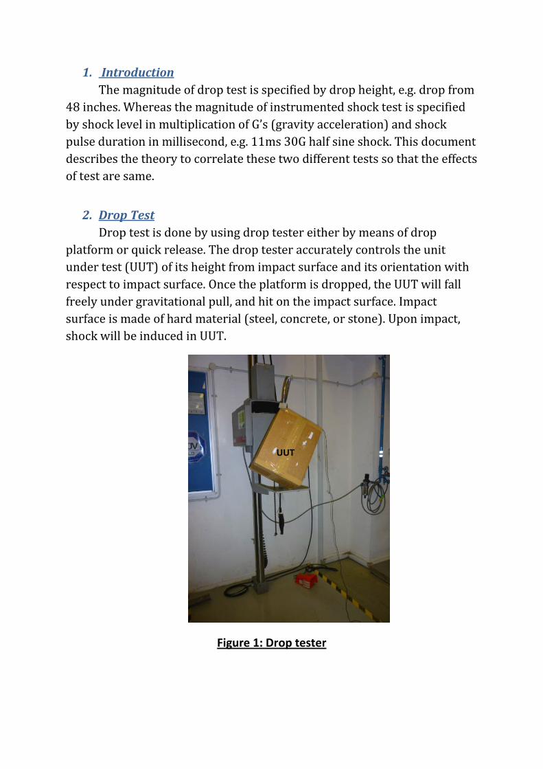
2. Drop Test Drop test is done by using drop tester either by means of drop

platform or quick release. The drop tester accurately controls the unit under test (UUT) of its height from impact surface and its orientation with respect to impact surface. Once the platform is dropped, the UUT will fall freely under gravitational pull, and hit on the impact surface. Impact surface is made of hard material (steel, concrete, or stone). Upon impact, shock will be induced in UUT.

Figure 1: Drop tester

UUT

3. Instrumented Shock Test Instrumented shock test is usually used to test the fragility of UUT.

The shock machine has a mount table where UUT can be secured to. The table is guided to move vertically, the input shock pulses are programmed accurately; they are carefully monitored and corrected throughout the whole shock test via accelerometers (Figure 2)mounted to the table in closed loop manner, so it can be controlled to be repeatable. And the response of UUT to the shock input will be monitored as well via accelerometers.

Figure 2: Typical accelerometer (L); UUT mounted with accelerometer (R).

Testing with shock machine involves mounting the UUT on the shock table, raising the table, and then allowing it to fall and strike the shock pulse programmers underneath. Various wave shapes of shock pulses can be programmed and generated by shock machine, e.g. half sine, square, saw tooth, etc.

There are 2 modes of shock machine,

i. Impact mode. Whereby the shock table with UUT on it will be moving and accelerating towards stationary impact plane.

ii. Impulse mode. Whereby the stationary UUT will be propelled by high force electro-dynamic shaker.

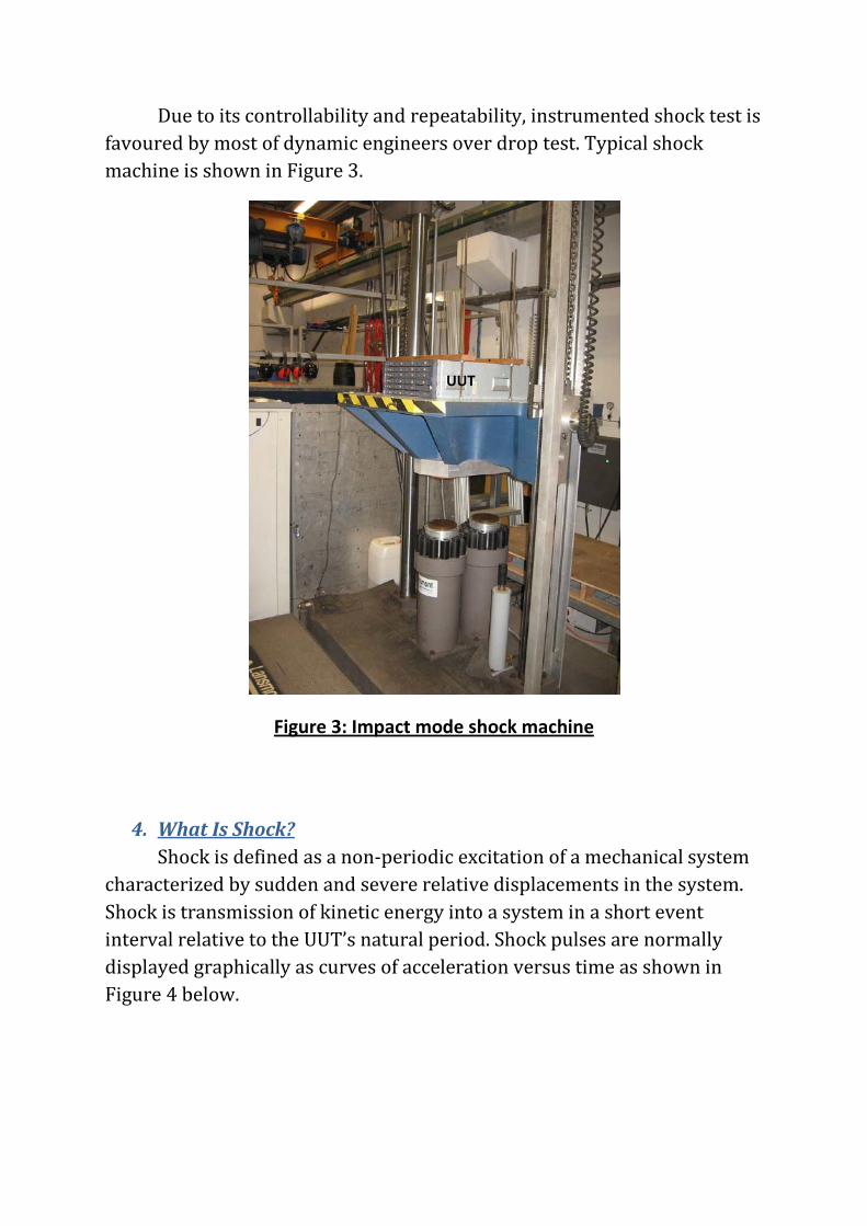
Due to its controllability and repeatability, instrumented shock test is favoured by most of dynamic engineers over drop test. Typical shock machine is shown in Figure 3.

Figure 3: Impact mode shock machine

4. What Is Shock? Shock is defined as a non-periodic excitation of a mechanical system

characterized by sudden and severe relative displacements in the system. Shock is transmission of kinetic energy into a system in a short event interval relative to the UUT’s natural period. Shock pulses are normally displayed graphically as curves of acceleration versus time as shown in Figure 4 below.

UUT

Figure 4: Half-sine shock pulse curve

5. Conservation of Energy in Free Fall Drop During free fall drop, potential energy PE1 of UUT will be converted

to kinetic energy KE1, and negligible heat energy loss due to air friction. During impact, some of the kinetic energy KE1 will be converted to heat and sound energy; and some will be dissipated into the system (falling UUT and impact surface). The energy is dissipated through system compression and expansion under tremendous action and reaction force; and the rest will be converted to kinetic energy KE2 should the UUT rebound. During rebound, the remnant kinetic energy KE2 will be converted to potential energy PE2 and negligible heat energy loss due to air friction.

As summary:

• During drop, PE1 = KE1 + heat loss • During impact, KE1 = KE2 + (Energy dissipated) + Sound + Heat • During bounce, KE2 = PE2 + heat loss

From second equation, we know KE2 < KE1 due to “Energy dissipated”, sound and heat energy loss. And the “Energy dissipated” is the factor that does real damage to the UUT and impact surface.

Energy dissipated, Ed =KE1 – KE2 – sound – heat.

Heat and sound energy can be neglected in our calculation.

Hence, Ed =KE1 – KE2

𝑬𝒅 = 𝟏𝟐𝒎(𝒗𝒊𝟐 − 𝒗𝒓𝟐) ---------------- (1)

Introducing parameters:

Velocity change, ∆𝒗 = |𝒗𝒊| + |𝒗𝒓| ---------------- (2)

Coefficient of restitution, 𝜺 = |𝒗𝒓||𝒗𝒊|

---------------- (3)

Substitute (2) and (3) into (1), and rearrange will gives

𝑬𝒅 = 𝟏𝟐𝒎(∆𝒗)𝟐 � 𝟏−𝜺

𝟏+𝜺 � -------------- (4)

From equation (4), energy dissipated Ed is proportional to velocity change ∆v. So velocity change ∆v determines the damage that will be done to the UUT. For correlating free fall drop test to instrumented shock test, ∆v will be used as parameter for correlation. Thus level of damage in drop test and shock test can be correlated.

But one must bear in mind that velocity change ∆v is not the only factor that dictates whether or not the UUT will be damaged. The other dictating factor is the shock level A. These two factors are usually related and depicted in “Damage Boundary Curve” in product fragility analysis as shown in Figure 5.

It is a plot of the damage causing parameters of a shock pulse and defines the region where certain combinations of acceleration and velocity change will cause damage. This curve is constructed by conducting series of drop/shock test with increasing shock level and velocity change to determine the critical velocity change ∆vc and critical shock level Ac . It is usually used by packaging engineer to design cost effective packaging.

Figure 5: Damage boundary curve.

From Figure 5 above, damage will only happen to UUT when the velocity change exceeds its critical value ∆vc , and shock level also exceeds its critical value Ac . If the combination of shock level and velocity change fall outside of the damage region, no damage will occur. For example if a product experiences a shock impact whereby the shock level reaches 1000g, but the velocity change is lower than ∆vc, no damage will be imposed on the product. This could be indication of over-packaging.

The other scenario where no damage occurs is when product experiences shock impact whereby the velocity change exceeded ∆vc , but shock level is lower than Ac . This is an indication of sufficient packaging that provides good cushioning in which the pulse duration τ is prolonged, that leads to decrease in shock level A, although velocity change has already exceeded ∆vc .

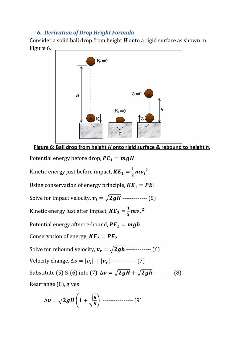
6. Derivation of Drop Height Formula Consider a solid ball drop from height H onto a rigid surface as shown in Figure 6.

Figure 6: Ball drop from height H onto rigid surface & rebound to height h.

Potential energy before drop, 𝑷𝑬𝟏 = 𝒎𝒈𝑯

Kinetic energy just before impact, 𝑲𝑬𝟏 = 𝟏𝟐𝒎𝒗𝒊𝟐

Using conservation of energy principle, 𝑲𝑬𝟏 = 𝑷𝑬𝟏

Solve for impact velocity, 𝒗𝒊 = �𝟐𝒈𝑯 ------------- (5)

Kinetic energy just after impact, 𝑲𝑬𝟐 = 𝟏𝟐𝒎𝒗𝒓𝟐

Potential energy after re-bound, 𝑷𝑬𝟐 = 𝒎𝒈𝒉

Conservation of energy, 𝑲𝑬𝟐 = 𝑷𝑬𝟐

Solve for rebound velocity, 𝒗𝒓 = �𝟐𝒈𝒉 ------------- (6)

Velocity change, ∆𝒗 = |𝒗𝒊| + |𝒗𝒓| ------------- (7)

Substitute (5) & (6) into (7), ∆𝒗 = �𝟐𝒈𝑯 + �𝟐𝒈𝒉 ---------- (8)

Rearrange (8), gives

∆𝒗 = �𝟐𝒈𝑯�𝟏 + �𝒉𝑯� ---------------- (9)

τ

H

h

Vi Vr

V0 =0

Vf =0

Vm =0

∆𝒗 = �𝟐𝒈𝑯(𝟏+ 𝜺) --------------- (10)

Where coefficient of restitution, 𝜺 = |𝒗𝒓||𝒗𝒊|

= �𝒉𝑯

;𝟎 < 𝜺 < 𝟏.

If ε = 0, means perfectly inelastic impact. If ε = 1, means perfectly elastic impact. Usually ε is in the range of 0.25~0.751

Solve (10) for drop height, 𝑯 = 𝟏𝟐𝒈� ∆𝒗𝟏+𝜺

�𝟐

-------------- (11)

.

From equation (11), if value of velocity change ∆v, and coefficient of restitution ε are known, drop height H, or known as “effective free fall drop height” EFFDH, can be determined.

7. Velocity Change ∆v Velocity change ∆v can be determined from area under the shock response curve.

For trapezoidal shock, velocity change is area under the curve in Figure 7.

Figure 7: Ideal trapezoidal shock pulse.

1 http://www.lansmont.com/SixStep/Step_2.htm

Shock level [G]

A

0 τ Pulse [ms]

Velocity change =190ips with 10% rise and fall times (minimum 170ips)

Usually for trapezoidal shock, the velocity change will be specified, e.g. 50G’s 190ips trapezoidal shock. So the velocity change here is 190ips (inch per second). This value can be directly input into equation (11).

For half sine shock, velocity change is area under the curve in Figure 8.

Figure 8. Ideal half sine shock pulse.

Since the half sine shock level (e.g. 10ms of 50G’s half sine shock) does not specify the velocity change requirement directly, but it can be found either by numerical method, or analytical integration as below.

Velocity change, ∆𝒗 = ∫ 𝑨 𝐬𝐢𝐧(𝝎𝒕) 𝒅𝒕𝝉𝟎 ------------- (12)

Where angular velocity, 𝝎 = 𝟐𝝅𝒇; and pulse duration, 𝝉 = 𝟏𝟐𝒇

; 𝑨 = shock

level.

Solving (12), gives ∆𝒗 = 𝟐𝑨𝝉𝝅

----------- (13)

So EFFDH can be found by substituting (13) into (11), EFFDH

𝑯 = 𝟐𝒈� 𝑨𝝉𝝅(𝟏+𝜺)

�𝟐

--------------- (14) for half sine shock

From equation (14), EFFDH can be determined with given shock level A and pulse duration τ. For FEA drop simulation, value ε = 0 should be used. See section 8.

Shock level [G]

A

0 τ Pulse [ms]

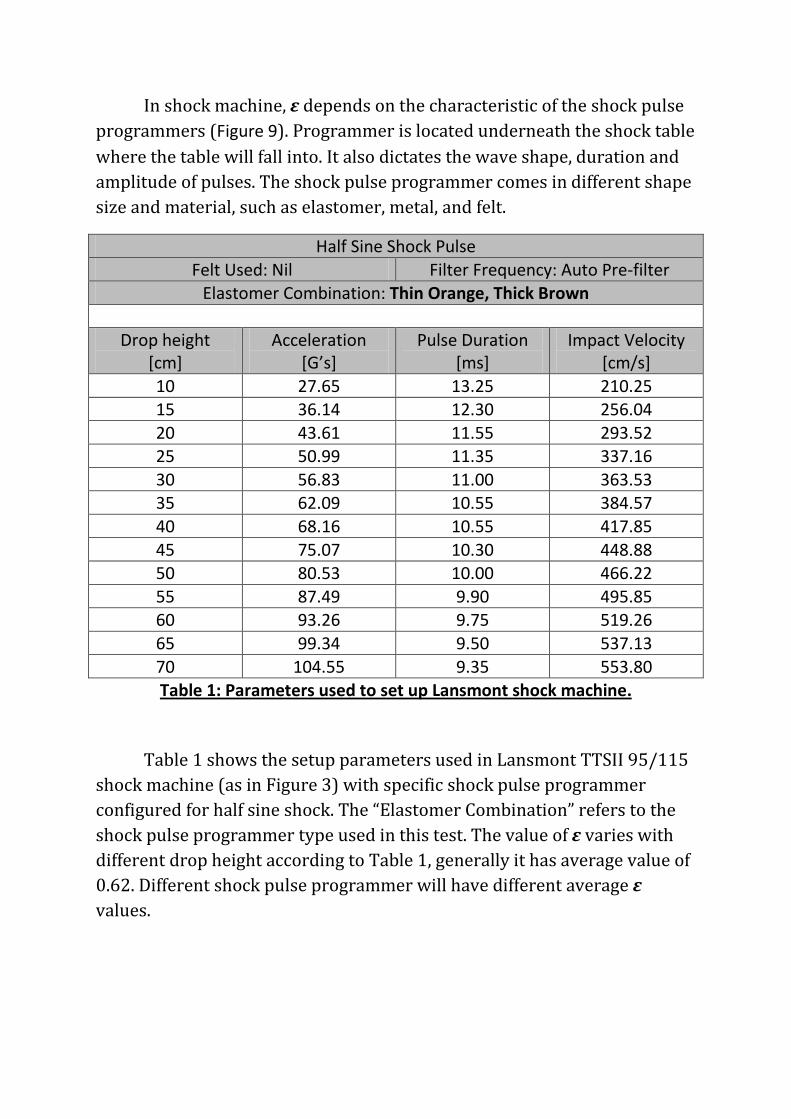
In shock machine, ε depends on the characteristic of the shock pulse programmers (Figure 9). Programmer is located underneath the shock table where the table will fall into. It also dictates the wave shape, duration and amplitude of pulses. The shock pulse programmer comes in different shape size and material, such as elastomer, metal, and felt.

Half Sine Shock Pulse Felt Used: Nil Filter Frequency: Auto Pre-filter

Elastomer Combination: Thin Orange, Thick Brown

Drop height [cm]

Acceleration [G’s]

Pulse Duration [ms]

Impact Velocity [cm/s]

10 27.65 13.25 210.25 15 36.14 12.30 256.04 20 43.61 11.55 293.52 25 50.99 11.35 337.16 30 56.83 11.00 363.53 35 62.09 10.55 384.57 40 68.16 10.55 417.85 45 75.07 10.30 448.88 50 80.53 10.00 466.22 55 87.49 9.90 495.85 60 93.26 9.75 519.26 65 99.34 9.50 537.13 70 104.55 9.35 553.80 Table 1: Parameters used to set up Lansmont shock machine.

Table 1 shows the setup parameters used in Lansmont TTSII 95/115 shock machine (as in Figure 3) with specific shock pulse programmer configured for half sine shock. The “Elastomer Combination” refers to the shock pulse programmer type used in this test. The value of ε varies with different drop height according to Table 1, generally it has average value of 0.62. Different shock pulse programmer will have different average ε values.

Figure 9: Typical shock pulse programmer.

8. CoR ε = 0 or ε = 1 in FEA? In FEA simulation, the value of ε of impact plane is hard to set, if not

unable to be set. So what is the value of ε to be used in order to find EFFDH by using equation (11)?

From equation (10), ∆𝑣 = �2𝑔𝐻(1 + 𝜀), one could deduce that “maximum” velocity change happens when ε =1,

∆𝒗𝒎𝒂𝒙 = 𝟐�𝟐𝒈𝑯∆𝒗𝒎𝒂𝒙 ---------------- (15)

Whereas “minimum” velocity change happens when ε = 0,

∆𝒗𝒎𝒊𝒏 = �𝟐𝒈𝑯∆𝒗𝒎𝒊𝒏 ---------------- (16)

At a glance it seems like ∆𝒗𝒎𝒂𝒙 > ∆𝒗𝒎𝒊𝒏 , but it is not.

From equation (14), if ε = 1,

𝑯∆𝒗𝒎𝒂𝒙 = 𝟏𝟐𝒈�𝑨𝝉𝝅�𝟐

------------ (17)

Similarly, if ε = 0,

𝑯∆𝒗𝒎𝒊𝒏 = 𝟐𝒈�𝑨𝝉𝝅�𝟐

-------------- (18)

Comparing (15) to (16), yield 𝑯∆𝒗𝒎𝒊𝒏 = 𝟒𝑯∆𝒗𝒎𝒂𝒙 --------------- (19)

Substitute (17) into (16), yield

∆𝒗𝒎𝒊𝒏 = �𝟐𝒈�𝟒𝑯∆𝒗𝒎𝒂𝒙�

∆𝒗𝒎𝒊𝒏 = 𝟐�𝟐𝒈𝑯∆𝒗𝒎𝒂𝒙 -------------- (20)

Comparing (20) to (15), ∆𝒗𝒎𝒊𝒏 = ∆𝒗𝒎𝒂𝒙 -------------- (21)

From equation (21), regardless of the value of ε, the velocity change ∆v is the same. This is because of the ∆v is characterized by shock level A and pulse duration τ.

Conservatively, value ε = 0 should be used to get the maximum EFFDH. Since in FEA environment, we do not know the impact plane would have elastic or inelastic impact property.

9. Summary • Equation (11) is used to determine equivalent free fall drop height

that has equivalent velocity change to an instrumented shock. • For FEA drop simulation, the value of coefficient of restitution ε

should be set to 0 as worst case scenario.

-- End of Document --