Western Australian Telecommunications Research Institute

Correlation between Near Field and Far Field Radiated Emission of Printed Circuit Boards

by Genetic Algorithms

Hongmei Fan (BEng, MEng)

This thesis is presented for the degree of

Doctor of Philosophy of

The University of Western Australia.

School of Electrical, Electronic and Computer Engineering

The University of Western Australia

Crawley, WA 6009, Australia

June 2009

i

Abstract

Most electromagnetic interference standards specify that measurements of radiated

emissions must be performed in the far field (FF), e.g. at an open-area test site or in a

semi-anechoic chamber. Since near field (NF) measurements are cheaper, quicker and

more flexible compared to FF tests, establishing a correlation between NF and FF data

is of great research interest. One strategy to achieve this goal is to find a set of basic

radiators comprising electric and magnetic dipoles that generate the same NF as the

original source at selected observation points. This set of dipoles, based on the

uniqueness theorem, can then be used to predict the FF radiation patterns.

The uniqueness theorem requires that electric or magnetic fields are matched on a

closed surface with respect to the magnitude and phase. The focus of this thesis is the

investigation of FF prediction based on NF magnitude-only data.

In this thesis, a robust NF-FF conversion model based on Genetic Algorithms (GAs) is

built up to predict the radiation of printed circuit boards (PCBs). This is done by

introducing a dipole moment magnitude range pre-selection before the initialisation step

of GAs, customising the processes of selection, crossover and mutation for anti-sticking

and checking the correlation between NF and FF fitness values.

Since the performance of GAs is tightly related to the number of dipoles in the GA

model, FF characteristics of generic radiation sources (such as a long wire and a large

loop) are analysed using both analytical calculation and source modelling by GAs. For

structures with simple FF patterns, if more dipoles than necessary are used, the

computational cost of GAs is unnecessarily high. On the other side, for structures with

complicated FF patterns, the GA modelling may not be able to well approximate the FF

radiation, due to the limitation for GAs to tackle too many unknowns. Therefore the

scope of the model applicability is discussed, and a dipole number N, depending on the

electrical size of the source, is recommended for GA modelling.

By applying GAs to get the equivalent dipole set of a radiating PCB from the magnetic

NF magnitudes, NF sampling approaches are investigated in detail, including where to

locate NF sampling planes, what plane coverage angle to choose, how many points to

observe, what type of data to collect, what dynamic range to allow for the data, and how

many planes to choose.

ii

Two case studies are presented for predicting the FF radiation of PCBs from magnetic

NF magnitude-only observations, and validate the NF sampling approaches in this

thesis.

iii

Table of Contents

Abstract ..............................................................................................i

Table of Contents ............................................................................. iii

Acknowledgements ......................................................................... vii

1 Introduction ............................................................................... 1

1.1 Background .........................................................................................................1

1.2 Near Field-Far Field Conversion Techniques.....................................................2

1.2.1 Modal Expansion Method.........................................................................3

1.2.2 Finite Element Method..............................................................................3

1.2.3 Equivalent Current Approach ...................................................................3

1.2.4 Phase Retrieval Technique........................................................................4

1.2.5 Equivalent Dipole Set Approach...............................................................6

1.3 Genetic Algorithms.............................................................................................8

1.4 Motivation...........................................................................................................9

1.5 Thesis Outline ...................................................................................................10

1.6 Summary of Contributions................................................................................10

2 Genetic Algorithms.................................................................. 166H12

16H2.1 Terminology...................................................................................................... 167H13

17H2.2 Genes and Parameter Ranges............................................................................ 168H13

18H2.3 Initialisation ...................................................................................................... 169H14

19H2.3.1 Moment Range Pre-selection .................................................................. 170H15

20H2.3.2 Example .................................................................................................. 171H18

21H2.4 Reproduction..................................................................................................... 172H20

22H2.4.1 Selection.................................................................................................. 173H21

23H2.4.2 Crossover ................................................................................................ 174H23

24H2.4.3 Mutation .................................................................................................. 175H25

25H2.5 Evaluation of Genetic Algorithms .................................................................... 176H27

26H2.5.1 Source Identification ............................................................................... 177H27

27H2.5.2 Fitness Definition.................................................................................... 178H29

iv

2.5.2.1 Near Field Tolerance....................................................................... 179H30

29H2.5.2.2 Far Field Tolerance ......................................................................... 180H31

30H2.5.2.3 Near Field-Far Field Tolerance Correlation ................................... 181H32

31H2.5.3 Optimum Fitness Model ......................................................................... 182H34

32H2.5.4 Evolution Process of Genes .................................................................... 183H36

33H2.5.5 Algorithm Repeatability.......................................................................... 184H38

34H3 Source Modelling of Far Field Radiation.................................. 185H41

35H3.1 Definition of Far Field Region.......................................................................... 186H42

36H3.2 Far Field Decomposition .................................................................................. 187H43

37H3.2.1 Small Radiator......................................................................................... 188H43

38H3.2.2 Long Wire ............................................................................................... 189H45

39H3.2.3 Large Loop.............................................................................................. 190H50

40H3.3 Source Modelling by Genetic Algorithms ........................................................ 191H55

41H3.3.1 Long Wire ............................................................................................... 192H56

42H3.3.1.1 300 MHz – 1.2 GHz........................................................................ 193H57

43H3.3.1.2 1.5 GHz ........................................................................................... 194H60

44H3.3.2 Large Loop.............................................................................................. 195H67

45H3.3.3 Power-Ground Plane Pair ....................................................................... 196H69

46H3.4 Computational Cost of Genetic Algorithms ..................................................... 197H74

47H3.5 Number of Infinitesimal Dipoles ...................................................................... 198H75

48H4 Near Field Data Sampling Approaches ................................... 199H78

49H4.1 Investigated Configuration ............................................................................... 200H80

50H4.2 Definition of Near Field Region ....................................................................... 201H82

51H4.3 Dipole Location Margin.................................................................................... 202H84

52H4.4 Sampling Distance Comparison........................................................................ 203H89

53H4.5 Plane Coverage Angle ...................................................................................... 204H92

54H4.6 Data Type.......................................................................................................... 205H95

55H4.7 Number of Observation Points ......................................................................... 206H96

56H4.8 Number of Sampling Planes ............................................................................. 207H98

57H4.9 Number of Infinitesimal Dipoles .................................................................... 208H101

58H4.10 Dynamic Data Range .................................................................................... 209H106

59H4.11 Summary ....................................................................................................... 210H111

v

5 Near Field-Far Field Conversion Case Studies..................... 211H113

61H5.1 Microstrip Trace.............................................................................................. 212H113

62H5.1.1 Investigated Configuration.................................................................... 213H114

63H5.1.2 Image Theory ........................................................................................ 214H114

64H5.1.3 Near Field-Far Field Conversion .......................................................... 215H116

65H5.1.3.1 Input Characteristics ..................................................................... 216H116

66H5.1.3.2 Near Field Region Sampling Comparison .................................... 217H117

67H5.1.3.3 Field Patterns................................................................................. 218H119

68H5.2 Electrically Large Loop .................................................................................. 219H122

69H5.2.1 Magnetic Near Field Testing by EMSCAN.......................................... 220H122

70H5.2.2 Electric Far Field Testing in Chamber .................................................. 221H125

71H5.2.3 Near Field-Far Field Conversion .......................................................... 222H126

72H5.2.3.1 Equivalent Dipole Set ................................................................... 223H127

73H5.2.3.2 Near Field Matching ..................................................................... 224H128

74H5.2.3.3 Far Field Prediction....................................................................... 225H129

75H6 Conclusions and Future Work............................................... 226H131

76H6.1 Conclusions..................................................................................................... 227H131

77H6.1.1 Robust Genetic Algorithm Model......................................................... 228H131

78H6.1.2 Number of Infinitesimal Dipoles .......................................................... 229H132

79H6.1.3 Near Field Sampling Approaches ......................................................... 230H132

80H6.1.4 Near Field-Far Field Conversion Case Studies..................................... 231H133

81H6.2 Future Work .................................................................................................... 232H133

82H6.2.1 Image Processing for Far Field Pattern Comparison ............................ 233H133

83H6.2.2 Near Field Test Probe Array ................................................................. 234H134

84H6.3 Outlook ........................................................................................................... 235H134

85HAppendix A Glossary .................................................................... 236H135

86HA.1 Abbreviations ................................................................................................ 237H135

87HA.2 Symbols and Parameters ............................................................................... 238H135

88HAppendix B List of Figures and Tables......................................... 239H139

89HB.1 List of Figures ............................................................................................... 240H139

90HB.2 List of Tables................................................................................................. 241H142

vi

Appendix C Dipole Field Calculation.............................................144

C.1 Infinitesimal Electric Dipole Field................................................................144

C.2 Infinitesimal Magnetic Dipole Field .............................................................147

C.2.1 Field of Loop Lying on the X-Y Plane .................................................. 147

C.2.2 Field of Loop Lying on the Y-Z Plane................................................... 150

C.2.3 Field of Loop Lying on the Z-X Plane .................................................. 152

C.2.4 Field of Loop Rotating from any Point.................................................154

Appendix D Field Decomposition for Chapter 3 ............................157

D.1 Far Field of Long Wire ................................................................................. 157

D.1.1 Half Wavelength Wire ..........................................................................157

D.1.2 One Wavelength Wire...........................................................................158

D.1.3 One and Half Wavelength Wire............................................................158

D.1.4 Double Wavelength Wire...................................................................... 159

D.1.5 Two and Half Wavelength Wire ...........................................................159

D.2 Far Field of Large Loop ................................................................................ 160

D.2.1 General Case ......................................................................................... 160

D.2.2 Special Case .......................................................................................... 163

Appendix E Field Tolerances for Chapter 4 ..................................167

E.1 Dipole Location Margin................................................................................167

E.2 Sampling Distance Comparison.................................................................... 171

E.3 Plane Coverage Angle................................................................................... 173

E.4 Data Type...................................................................................................... 175

E.5 Number of Observation Points...................................................................... 177

E.6 Number of Sampling Planes ......................................................................... 179

Appendix F Author Biography .......................................................186

F.1 Author Publications ........................................................................................ 186

F.2 Awards Received ............................................................................................ 187

References....................................................................................188

vii

Acknowledgements

A great number of people have helped me in one way or another to finish the research

work presented in this thesis. In particular I would like to acknowledge:

My Supervisor, Dr. Franz Schlagenhaufer, the Electromagnetic Compatibility (EMC)

Research Group Leader at Western Australian Telecommunications Research Institute

(WATRI), for his expert guidance, rigorous and effective training, and prompt feedback

throughout the course of this research. He is a gifted theoretician in electromagnetic

field modelling and also an experienced practitioner in EMC troubleshooting, and I

consider myself very privileged to have had the opportunity to work with and learn

from him. In addition I would like to thank him for giving me the chance to be a tutor

and a lab demonstrator for the Electromagnetic Theory course at The University of

Western Australia (UWA), and also to be an assistant for his EMC seminars and

workshops conducted in China.

My Associate Supervisor, Prof. Kevin Fynn, for his valued assistance in the early stages

of this research, and for his support during the whole period.

The WATRI Research Director, Prof. Antonio Cantoni, for the many instructive

discussions and his professional guidance relating to my research work.

My EMC associates, Dr. Joe Trinkle, Dr. Matthew Wood, Mr. Bert Wong and Mr.

Frank Schroeder, for their generous help, advice and discussions on electromagnetic

simulations, electromagnetic field measurements, and applying theory to explain

practical issues.

The experts in Power Electronics at the School of Electrical, Electronic and Computer

Engineering (EECE), Dr. Herbert Iu and Dr. Lawrence Borle, for providing me the

opportunity to conduct tutorials and lab demonstrations for two courses at UWA,

Circuits and Electronic Systems, and Electromagnetics and Electromechanics.

My lecturers at UWA, Dr. Nancy Longnecker and Dr. Jan Dook, for their interesting,

systematic and practical teaching on Science Communication.

The professional writers, Dr. Cecily Scutt at Murdoch University, Dr. Krys Haq and Dr.

Michael Azariadis at UWA, for facilitating the valuable seminars on Thesis Writing.

My erudite colleague at WATRI, Dr. Tarith Devadason, for his cheerfully given help

and suggestions on professional writing and presentation.

viii

My lawyer friend, Miss Natalie Quek, for helping proofread the thesis otherwise many

errors would have been missed.

My workmates at WATRI, Shierly, Yangqun, Manora, Colin, Hooi Hua, Bu-tuong and

Greg, for their help and information.

My husband Shikun Zhan and our son Litao, who have given me an enormous amount

of support, encouragement, care and patience throughout my research.

My parents, parents-in-law, sisters and brother for their consistent support.

My other friends scattered throughout China, Australia, the USA, Canada, the

Netherlands, Germany and Italy for their useful information and encouragement.

Finally, I would also like to gratefully acknowledge the financial assistance from

WATRI, EECE, the Australian Postgraduate Award scheme, the EMC Society of

Australia, the Postgraduate Students’ Association at UWA and the UWA Grants for

Research Student Training.

1

1 Introduction

1.1 Background

With the rapid development of Super Large Scale Integrated (SLSI) Circuits and Public

Data Networks, electromagnetic emissions can cause significant problems and are

subject to regulations in many industrialised countries.

For achieving Electromagnetic Compatibility (EMC) solutions, a typical system

approach starts from building a model of an electronic product, then carrying out

analysis and simulations, and later conducting measurements to validate the model. For

an efficient product development it is important, that measurements are already

performed during early design stages so that models can be fine-tuned.

It is desirable to predict the electromagnetic behaviour of a product on the basis of

measurement results obtained from its prototype. Many EMC standards, e.g. Special

International Committee on Radio Interference (CISPR) 22 or Federal Communications

Commission (FCC) 15, require radiation measurements for finished products to be

performed in the far field (FF) region. Typically, a Semi-Anechoic Chamber (SAC) or

an Open Area Test Site (OATS) is used to measure radiated field strengths at 3, 10 or

30 m distances from the product at 30 MHz – 6 GHz.

Compared with FF testing, near field (NF) measurements (i.e. measurements closer to

the product) are cheaper, quicker and more flexible. Therefore establishing a correlation

between NF and FF radiation data attracts increasing research interest. In addition, the

NF-FF conversion techniques may help design engineers to understand the impact of

enclosures and other structures on the radiation characteristics of printed circuit boards

(PCBs) in early design stages.

Regarding NF testing, performing measurements closer to the source has the advantage

of stronger signals, smaller observation surfaces and less influence of the environment;

however, larger testing distance reduces the spatial resolution requirement for NF

testing probes. Thus a compromise should be taken when choosing NF testing distances

(see Section 4.4).

This thesis predicts FF radiation patterns from sources (e.g. PCBs) based on field data

obtained in the radiating NF region, except for the examples in Chapter 3 where FF

input data are directly used for source modelling. Due to the limitation of the NF-FF

2

conversion techniques in this thesis (see Section 3.5), the operating frequency is ranged

from 30 MHz to 3 GHz, and the PCB size is up to electrically moderate (the maximum

PCB diagonal D ≤ λ, λ is the wavelength in the medium between the PCB and

observation points, i.e. in most cases free space). Furthermore, in terms of practical

considerations (e.g. for arranging the NF testing on a lab bench), D is scoped to be

within 0.5 m.

NF data in this thesis mean the x-, y- and z- components of field magnitudes. Most of

the time, they are from simulated data by a Method-of-Moments field solver [1]; while

measurements are taken for the case study in Section 5.2.

In this thesis, the target of the NF-FF conversion is to predict FF radiation with

adequate accuracy. To measure whether a FF prediction is good enough, a FF tolerance

is defined by the difference of the maximum electric field magnitude at selected points

between the prediction and reference data (see Section 2.5.2.2). In this thesis for an

acceptable prediction, 1.5 dB is suggested to be the maximum allowable tolerance. This

number is somewhat arbitrary; it has been found to be achievable for most examples in

this thesis, but is better than requirements in some EMC standards. For instance, CISPR

16 requires the accuracy of field-strength measurement of a uniform field of a sine-

wave should be better than ± 3 dB.

1.2 Near Field-Far Field Conversion Techniques

NF-FF conversion techniques have been developed for more than 40 years. They were

initially used for antenna measurement transformations, and were later applied in PCB

radiation prediction. The techniques can be divided into 5 categories:

1) Analytical methods based on modal expansion [2][3];

2) Classical numerical methods based on the Green’s theorem [3][4] and finite

element method (FEM [5]);

3) More recently new numerical methods based on equivalent current approach and

Method of Moments (MoM [4][6]);

4) Phase retrieval techniques [7][8];

5) Equivalent dipole set approaches [9] -[13] .

The former four methods are focused on antenna measurements, while the latter one is

3

more suitable for PCB radiation prediction.

1.2.1 Modal Expansion Method

A classical NF-FF conversion technique has been applied for obtaining FF antenna

patterns by NF measurements since the 1960s. It is an analytical approach based on

wave (modal) expansions [2][3] using Fourier transform (spectral) techniques. The

magnitude and phase of the tangential electric field components radiated by a test

antenna are measured at regular intervals over a well-defined NF surface. These electric

field data are used to determine the magnitude and phase of an angular spectrum of

plane, cylindrical or spherical waves. The next step is to express the total field of the

test antenna in terms of modal expansions, and then evaluate the FF pattern.

Using NF measurements to predict FF behaviour by the modal expansion method makes

the extent of scanning areas much smaller, and also bypasses the FF measurement

requirements such as open range, good characterisation of the site attenuation, and

logistic problems. Furthermore, modal expansions can be made computationally

efficient. However, there are restrictions regarding the sampling rate when a Fourier

transform approach is used, and also the FF is accurately determined only over a

particular angular sector that is dependent on the measurement configuration.

1.2.2 Finite Element Method

Since the 1990s R. Laroussi [14][15] has developed a numerical algorithm for NF-FF

conversion, based on the Green’s theorem [3][4] and FEM [5]. It assumes that the field

measurements (magnitude and phase) are available around two concentric surfaces

enclosing the Device Under Test (DUT) and that the field can be interpolated between

the measurements positions on the surface and in the volume between them [15].

The algorithm is independent of the type of radiators, and affected only by the amount

and accuracy of the available data [14][15].

1.2.3 Equivalent Current Approach

Realising the restrictions on NF testing surfaces of the modal expansion method, since

the 1990s T. Sarkar et al [16]-[19] have investigated an alternative numerical method

for computing FF antenna patterns from NF measurements. The method utilises NF data

4

to determine equivalent magnetic current sources over a fictitious planar surface that

encompasses the antenna by an electric field integral equation, and these currents are

used to ascertain the FF. The foundation of this method is the surface equivalence

principle [2][3][4].

In [16]-[19], the MoM [4][6] procedure was used to transform the integral equation into

a matrix one. The matrix equation was solved using the conjugate gradient method, and

in the case of a non-quadratic matrix, a least-squares solution for the currents was found

without explicitly computing the normal form of the equation.

In [20], T. Sarkar tried a similar numerical method, obtaining equivalent electric current

sources by NF data. It was found that the equivalent magnetic current approach

provided always a better solution than the equivalent electric current approach, due to

the more ill conditioned matrix arising from the electric field operator [20].

In [21], J. J. Laurin extended the equivalent magnetic current approach to the case of

small-size printed antennas. The method was validated experimentally with single-

element and small array prototypes using measurements made in the reactive NF region

of the antennas [21].

All NF-FF conversion approaches mentioned in Sections 1.2.1-1.2.3 are based on

complete NF data (magnitude and phase). Usually the magnitude measurement for

antennas is not a critical point, whereas the determination of the phase is much more

cumbersome from the practical point of view, particularly when dealing with high

frequencies. Factors making high frequency NF phase measurements inaccurate

include: probe-positioning errors (especially along the direction perpendicular to the

scanning plane), temperature changes and the mechanical movement of the cables

connected to the receiver, and the stability and accuracy of the receiver. Thus NF-FF

conversion capable of using NF phaseless measurements is in demand.

1.2.4 Phase Retrieval Technique

Since the 1990s a phase retrieval technique [7][8] has been used in the NF-FF

conversion of antenna measurements. The phase retrieval technique has been widely

used in such areas as optics, astronomy, electron microscopy, remote sensing,

holographic imaging, etc. It is a numerical Fourier iteration method, which usually

exploits more than one measurement surface and involves the minimisation of a non-

quadratic objective functional. First initialise a value for FF, then use Fourier transform

5

to retrieve NF phase information; later a least squares fitting is performed in the NF

measured magnitude space, and a new FF value is obtained by inverse Fourier

transform. This iteration process is repeated until the FF values obtained by NF data on

different surfaces are less than a chosen threshold.

In [22], O. M. Bucci first discussed FF pattern determination from NF magnitude data

on two surfaces. The accuracy of the FF reconstruction results was found to be related

both to the distance between such surfaces and to some extent a priori information

concerning the NF phase and/or the radiating system. The information on the radiating

system relaxed the need of any information on the NF phase provided that the distance

between the measurement surfaces was large enough. In [23], phase information was

retrieved for simulated NF magnitudes on two cylindrical surfaces, In [24], the phase

retrieval algorithm was described in detail and confirmed by experimental results

concerning NF data from a shaped reflector at 9 GHz. In [25], the FF pattern and

antenna aperture holographic images of two waveguide-fed slot array antennas

produced from the phase retrieval algorithm were shown to have excellent agreement

with results produced using the measured NF magnitude and phase.

Compared with NF measurements of both magnitude and phase, phaseless

measurements can provide strong advantages in terms of setup cost. Firstly, a scalar

network analyser can be used as a receiver instead of an expensive vector network

analyser. Secondly, probe positioning errors can be better tolerated since the field

magnitude generally shows less spatial variations than the phase, thus making less

severe the mechanical requirements of the scanning equipment. Thirdly, less expensive

cables can be used. In [26], a low-cost magnitude-only NF measurement setup was

introduced, and the measured intensity of NF for a standard gain horn antenna radiating

at 15 GHz was numerically processed to determine the FF pattern.

In [27], a new technique for the antenna diagnostics from simultaneous measurements

of the voltage magnitudes received by two different probes moving over a single

scanning NF surface was presented. In [28], an effective NF-FF conversion technique

from truncated and inaccurate magnitude-only data was presented.

In [29], magnitude-only data was first linked with the equivalent magnetic current

approach for NF-FF conversion. For an aperture antenna operating at 12.625 GHz, it

was found that the source reconstruction and FF pattern results using NF magnitude

information on one scanning surface is worse than those using NF magnitude on two

6

surfaces, and much worse than those using both NF magnitude and phase.

1.2.5 Equivalent Dipole Set Approach

All NF-FF conversion techniques mentioned in Sections 1.2.1-1.2.4 are applied in the

antenna measurements area. Although there are many factors making antenna phase

measurements inaccurate as referred to in Section 1.2.3, it is still possible to obtain the

phase shift between transmitted and received signal by network analysers. However, in

measuring radiation from PCBs, a reference signal to measure phase may be difficult or

expensive to obtain. Therefore using NF phaseless data to predict FF radiation

behaviour of PCBs is of great practical value.

In the 1990s M. Wehr [9][10] developed a new method for modelling the radiation

source of a large radiator by several pairs of electric and magnetic dipoles which create

the same NF components in an anechoic chamber. It was stated that both magnitude and

phase of electric and/or magnetic fields were needed to find the dipole pairs. Different

from the numerical iteration method based on Fourier transform, this method is more

convenient to operate and more suitable for analysing irregular radiation sources like

PCBs. It is based on finding an equivalent set of elementary electric and magnetic

dipoles which model the actual radiating sources, and therefore radiate the same NF as

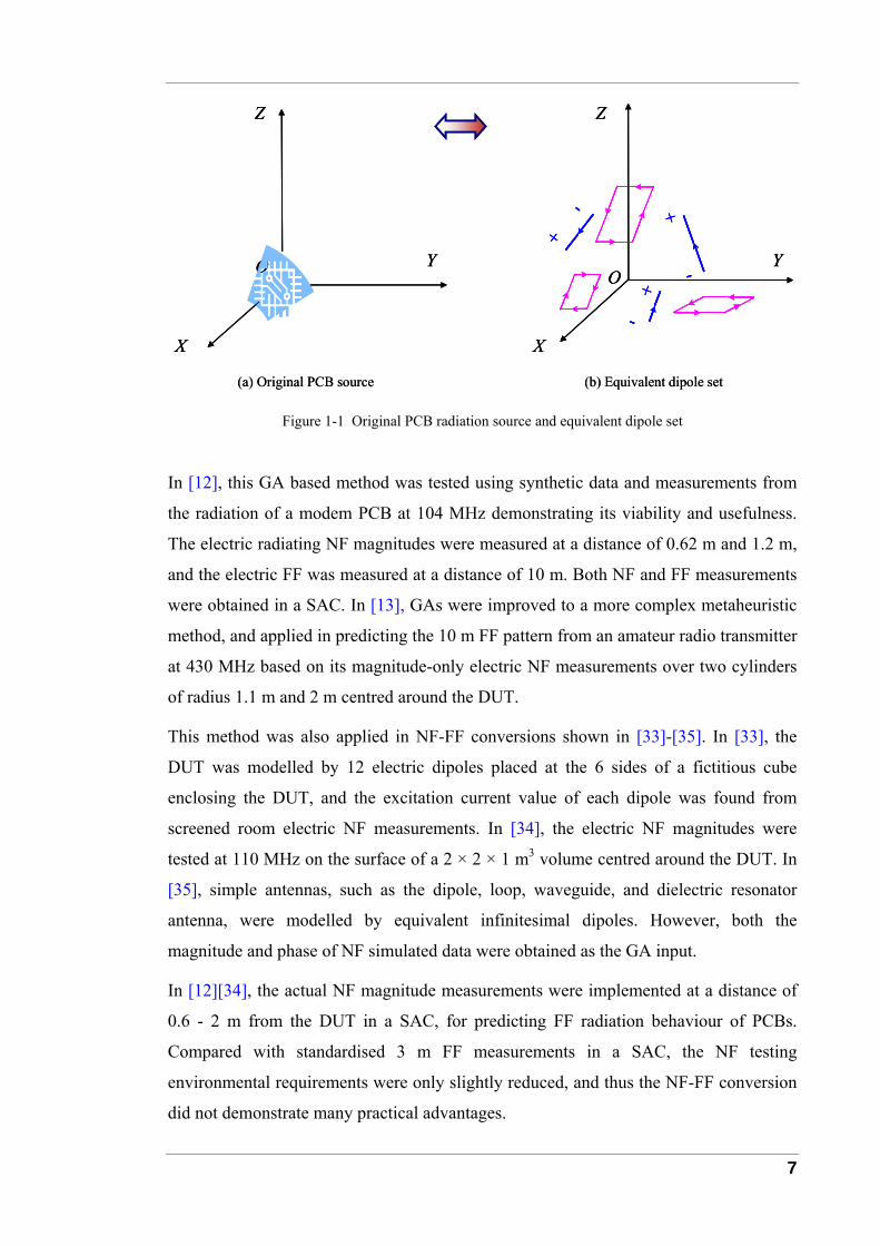
the original DUT (see Figure 1-1). Once the equivalent dipole set is found, the FF can

be easily computed analytically. The strategy was not only used for the radiator’s

characterisation [10], but also, under some circumstances, for the automatic detection of

the radiation leak [9]. Since the difficulty of the method was to select the correct

locations of the dipole pairs, an automatic program based on Evolution Strategies

(evolution processes taking place at the individual level [30]) was introduced [10].

Since 2000 J. Regue [11]-[13] has further developed the above method for source

identification and FF radiation prediction by NF magnitude-only measurements for PCB

characterisation instead of both NF magnitude and phase data. This is an extension of

applying the phase retrieval technique in the NF-FF conversion for radiation of PCBs.

Genetic Algorithms (GAs [30]-[32], evolution processes taking place at the genetic

level), a more robust global searching method especially suitable for dealing with

problems with incomplete information, are applied in this equivalent dipole set

approach. The application of GAs will be described in Section 1.3, and the detailed

process of GAs will be illustrated in Chapter 2.

7

Y+

-+

-+

-X

Z

O

X

Z

YO

(a) Original PCB source (b) Equivalent dipole set

Y+

-+

-+

-X

Z

OY

+-

+-

+

-

+

-+

-

+

-X

Z

O

X

Z

YO

X

Z

YO

(a) Original PCB source (b) Equivalent dipole set

Figure 1-1 Original PCB radiation source and equivalent dipole set

In [12], this GA based method was tested using synthetic data and measurements from

the radiation of a modem PCB at 104 MHz demonstrating its viability and usefulness.

The electric radiating NF magnitudes were measured at a distance of 0.62 m and 1.2 m,

and the electric FF was measured at a distance of 10 m. Both NF and FF measurements

were obtained in a SAC. In [13], GAs were improved to a more complex metaheuristic

method, and applied in predicting the 10 m FF pattern from an amateur radio transmitter

at 430 MHz based on its magnitude-only electric NF measurements over two cylinders

of radius 1.1 m and 2 m centred around the DUT.

This method was also applied in NF-FF conversions shown in [33]-[35]. In [33], the

DUT was modelled by 12 electric dipoles placed at the 6 sides of a fictitious cube

enclosing the DUT, and the excitation current value of each dipole was found from

screened room electric NF measurements. In [34], the electric NF magnitudes were

tested at 110 MHz on the surface of a 2 × 2 × 1 m3 volume centred around the DUT. In

[35], simple antennas, such as the dipole, loop, waveguide, and dielectric resonator

antenna, were modelled by equivalent infinitesimal dipoles. However, both the

magnitude and phase of NF simulated data were obtained as the GA input.

In [12][34], the actual NF magnitude measurements were implemented at a distance of

0.6 - 2 m from the DUT in a SAC, for predicting FF radiation behaviour of PCBs.

Compared with standardised 3 m FF measurements in a SAC, the NF testing

environmental requirements were only slightly reduced, and thus the NF-FF conversion

did not demonstrate many practical advantages.

8

1.3 Genetic Algorithms

This thesis is about predicting the FF radiation of PCBs based on NF magnitude-only

data. Similar as shown in [11]-[13], a GA based equivalent dipole set approach is

adopted.

Compared with other NF-FF techniques, such as the modal expansion method referred

to in Section 1.2.1 or the equivalent current approach mentioned in Section 1.2.3, the

equivalent dipole set approach by GAs is computationally less efficient, but has an

important advantage for this particular problem. When using GAs, it is sufficient to

know NF magnitude-only data; NF phase information is not required for FF prediction.

GAs are stochastic searching processes based on the Darwinian concepts of natural

selection and survival of the fittest. First proposed by John Holland in 1975 [36], and

later vastly improved by David Goldberg in the late 1980s [31], GAs have been an

attractive class of computational models. Particularly suitable for solving complex

optimisation problems, GAs have been applied in a wide variety of domains, such as

financial optimisation, manufacturing dispatch, automatic control, robotic intelligence

control, graphic process, pattern recognition, artificial life, genetic programming in

electronic circuit design, expert system, machine learning, biology, medicine etc [37].

Introduced into the realm of electromagnetic design in the early 1990s, GAs have

attracted researchers with diverse interests. Compared with local optimisation

techniques such as conjugate-gradient and quasi-Newton methods, GAs are classified as

global searching methods. Global techniques not only are largely independent of initial

conditions, but also place few constraints on the solution domain. Thus they are more

robust when faced with ill-behaved solution spaces, which have discontinuities,

constrained parameters, and/or a large number of dimensions with many potential local

optima [38]-[40].

The objective functions arising in electromagnetic optimisation problems are often

highly nonlinear, stiff, discontinuous, multi-extremal, and non-differentiable [38][40].

For such problems, especially for problems with incomplete information as an input,

with large probability GAs can yield globally optimum solutions that are not found by

using traditional local-search optimisation methods.

GAs have been successfully applied in the area of electromagnetics, such as the design

of antennas, electromagnetic filters and absorbers, the synthesis of magnetostatic

9

devices, as well as inverse scattering problems [38]-[40]. Especially in the design and

synthesis of antennas, GAs are extensively utilised to find a radiating structure that

meets a set of performance criteria, including gain, maximum side lobe level, beam

width, input impedance and physical size.

1.4 Motivation

Sections 1.2 and 1.3 introduced state of the art of NF-FF conversion techniques and

GAs, respectively. As mentioned in Section 1.2.5, the equivalent dipole set approach

based on GAs has been applied in cases where the operating frequencies were not too

high (104 – 430 MHz), and the NF testing distances were not too close (0.6 – 2 m). This

thesis adopts the equivalent dipole set approach, however aims to investigate the

correlation between NF magnitudes and FF prediction of PCB radiation under a wider

and more flexible application scope. As indicated in Section 1.1, the size of PCBs

considered is up to a wavelength, and the operating frequency range is 30 MHz – 3

GHz. Furthermore, from the practical point of view, the PCB size is limited to be within

0.5 m, and the NF testing is to be done on a work bench (testing distance r < 0.5 m).

To reach the above application target, the following questions arise and will later be

investigated in this thesis:

1) As mentioned in Section 1.1, the purpose of the NF-FF conversion is to predict

FF radiation. Since there are many ways to define the objective function for

checking the difference between reference NF data and the GA NF

approximation, which function is the best one for this NF-FF conversion case?

Does a good NF approximation mean good FF prediction?

2) Generally speaking, for a finite-sized PCB, complexity of the FF radiation

pattern increases with the operating frequency. Using GAs to search for the

equivalent infinitesimal electric and magnetic dipoles which share the same NF

data with the original PCB, more dipoles are possibly needed for higher

frequencies. However, a larger dipole number means more unknown parameters

to tackle, and thus leads to longer computation time. Furthermore, for very

complicated FF patterns, the GA model may not be able to find the global

optimum solution, due to GA’s residual tendency to get stuck to local optima

like any other optimisation methods. Thus how to select the number of

10

infinitesimal dipoles in the GA model? Is there any practical limitation for the

NF-FF conversion model?

3) There have been many various definitions of NF and FF regions for different

applications. What do NF and FF regions mean in this NF-FF conversion case?

What are the boundaries of them? Are they related to the PCB size? Regarding

NF data sampling, where should the testing be done? What type of data to

collect? How many points to test? For some NF observation points, some of the

field components are very small compared with the test probe sensitivity. Is it

necessary to manipulate those small components? Will it influence the final FF

prediction results? Only after these questions are answered can a clear guideline

be drafted for the NF scanning machine design.

1.5 Thesis Outline

This thesis consists of 6 chapters. Chapter 1 gives a brief introduction of NF-FF

conversion techniques, emphasises the aim and strategy of the thesis, and summarises

the contribution of the thesis. Chapter 2 builds up a NF-FF conversion model based on

GAs. Chapter 3 is about source modelling of FF radiation, which gives suggestions on

choosing the optimum number of dipoles needed by the GA model. Chapter 4 discusses

in detail NF sampling approaches. Chapter 5 contains some case studies of PCB FF

radiation prediction based on NF simulations and measurements. Chapter 6 provides

conclusions and suggestions for future work.

1.6 Summary of Contributions

There are four contributions in this thesis. The first is construction of a NF-FF

conversion model based on GAs. The second is a recommendation for an appropriate

infinitesimal dipole number for the GA model based on the FF radiation evaluation. The

third is investigations of reasonable NF sampling approaches. The last is some practical

case studies on NF-FF conversion.

Robust Genetic Algorithm Model

A GA model including a specific dipole moment range pre-selection step is constructed

for NF-FF conversion. Four original dipoles (2 electrical and 2 magnetic) at 30 MHz in

free space are selected as a known source to check whether the GAs can identify the

11

original radiator. It elaborates how the GA works, how the genes evolute with iteration,

how they converge to an optimum solution, and what the correlation is between the NF

tolerance and FF tolerance.

Number of Infinitesimal Dipoles

By applying GAs to reconstruct the FF patterns of a long wire, a large loop and a

power-ground plane pair, the correlation between the number of infinitesimal dipoles

needed by GAs and the ratio of PCB size over wavelength (D/λ) is discussed. In this

thesis, it is found that the GAs work well when the dipole number is no more than 8.

For PCBs with D ≤ λ, a number of infinitesimal dipole is recommended for GA

modelling.

Near Field Sampling Approaches

A 90 mm × 60 mm PCB with an L-shape loop above a finite ground plane is

investigated using different NF sampling approaches. This example produces highly

asymmetrical FF patterns for high frequencies (1 GHz – 3 GHz), while very simple and

symmetrical patterns for low frequencies (30 – 300 MHz) due to its small size.

• A few regions are clearly defined by the increasing distance from the PCB

source. For electrically moderate-sized PCBs, NF data sampled in the radiating

NF region is recommended for NF-FF conversion.

• Detailed NF planar sampling approaches are investigated, such as where to

place observation points, what type of data to observe, how many points to

sample, how many surfaces to select, how big the spacing between sampling

points should be, and how to deal with very small field values.

Near Field-Far Field Conversion Case Study

Two case studies are conducted to predict electric FF patterns based on magnetic NF

magnitudes, one for a 210 mm × 2.5 mm microstrip trace on a 250 mm × 45 mm × 1.57

mm PCB at 300 MHz – 1.2 GHz, and the other for an 80 mm × 60 mm loop at 500

MHz. Both cases validate the NF sampling approaches in this thesis.

12

2 Genetic Algorithms

This chapter serves to introduce a GA which is applied to search the optimum

equivalent dipole set, for predicting FF behaviour based on NF data. A GA based NF-

FF conversion model is built, and its performance related to source identification,

fitness definition, genes evolution and algorithm repeatability is evaluated in detail.

Outline

This chapter is organised into 5 sections. Section 2.1 lists some GA terms. Section 2.2

defines hybrid-coding genes including the dipole type, complex moment, location and

orientation. Section 2.3 introduces a dipole moment magnitude range pre-selection

which is applied in the initialisation step of GAs. Section 2.4 draws a detailed picture

about the reproduction stage of GAs, which contains important steps such as selection,

crossover and mutation. The purpose of these manipulations is to find a global optimum

by avoiding sticking at local optima. Section 2.5 evaluates the effectiveness of GAs in

this NF-FF conversion case, by checking the feasibility of identifying a radiation source

based on NF magnitude-only data, trying different fitness definitions, looking for the

optimum fitness model, illustrating the evolution process of genes, and analysing the

repeatability of GA runs.

Contributions

The contributions of this chapter are:

1) Before the first usual step of GAs—initialisation, a pre-selection process for the

dipole moment range is introduced, based on analysing all available NF data.

2) During the reproduction step, processes of selection, crossover and mutation are

customised for anti-sticking, and thus improving the robustness and

repeatability of GAs.

3) Fitness definitions of NF matching and FF prediction are investigated, and the

correlation between NF and FF fitness is analysed.

4) The evolution of some genes and NF-FF fitness correlation is illustrated, which

helps understand how the GA works in the NF-FF conversion.

13

2.1 Terminology

To help understand GAs, some terms are briefly explained as follows [39][40]:

• Gene: a specific variable of a solution.

• Code: a format representing genes. There are a few coding methods, such as

binary, Gray and real-coding.

• Individual: a trial solution to the problem, represented by a string of genes.

• Population: a set of possible solutions to a given problem, a group of individuals.

• Generation: one iteration cycle in a GA process.

• Fitness: a number assigned to an individual, representing how good a solution to

the problem it is. The higher the fitness, the more chances to be chosen as a

parent for the next generation.

• Parent: member of the current generation. Pairs of individuals are selected from

the population in a probabilistic manner weighted by their relative fitness values

and designated as parents.

• Offspring: member of the next generation, generated from the selected pair of

parents by application of stochastic operators.

2.2 Genes and Parameter Ranges

An individual is a set of N elementary dipoles, where each dipole Dq (q=1, 2, …, N) is

characterised by [42]-[49]:

• Dipole type Kq (binary-coded, ‘0’ for a magnetic dipole, ‘1’ for an electric

dipole),

• Complex dipole moment qjqm e β⋅ ,

• Dipole location xq, yq, zq, and

• Dipole orientation θq, φq (elevation and azimuth angle),

where the dipole location and orientation in both local (O’X’Y’Z’) and global (OXYZ)

coordinate systems are as shown in Figure 2-1.

14

X’

Z’

Y’O’

X

Y

Z

O

O’=(xq, yq, zq) in OXYZ coordinate system

θq

ϕq

+

-

X’

Z’

Y’O’

X

Y

Z

O

O’=(xq, yq, zq) in OXYZ coordinate system

θq

ϕq

+

-

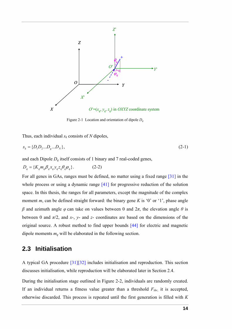
Figure 2-1 Location and orientation of dipole Dq

Thus, each individual sk consists of N dipoles,

,...... 21 Nqk DDDDs = (2-1)

and each Dipole Dq itself consists of 1 binary and 7 real-coded genes,

.q q q q q q q q qD K m x y zβ θ ϕ= (2-2)

For all genes in GAs, ranges must be defined, no matter using a fixed range [31] in the

whole process or using a dynamic range [41] for progressive reduction of the solution

space. In this thesis, the ranges for all parameters, except the magnitude of the complex

moment m, can be defined straight forward: the binary gene K is ‘0’ or ‘1’, phase angle

β and azimuth angle φ can take on values between 0 and 2π, the elevation angle θ is

between 0 and π/2, and x-, y- and z- coordinates are based on the dimensions of the

original source. A robust method to find upper bounds [44] for electric and magnetic

dipole moments mq will be elaborated in the following section.

2.3 Initialisation

A typical GA procedure [31][32] includes initialisation and reproduction. This section

discusses initialisation, while reproduction will be elaborated later in Section 2.4.

During the initialisation stage outlined in Figure 2-2, individuals are randomly created.

If an individual returns a fitness value greater than a threshold Fthr, it is accepted,

otherwise discarded. This process is repeated until the first generation is filled with K

15

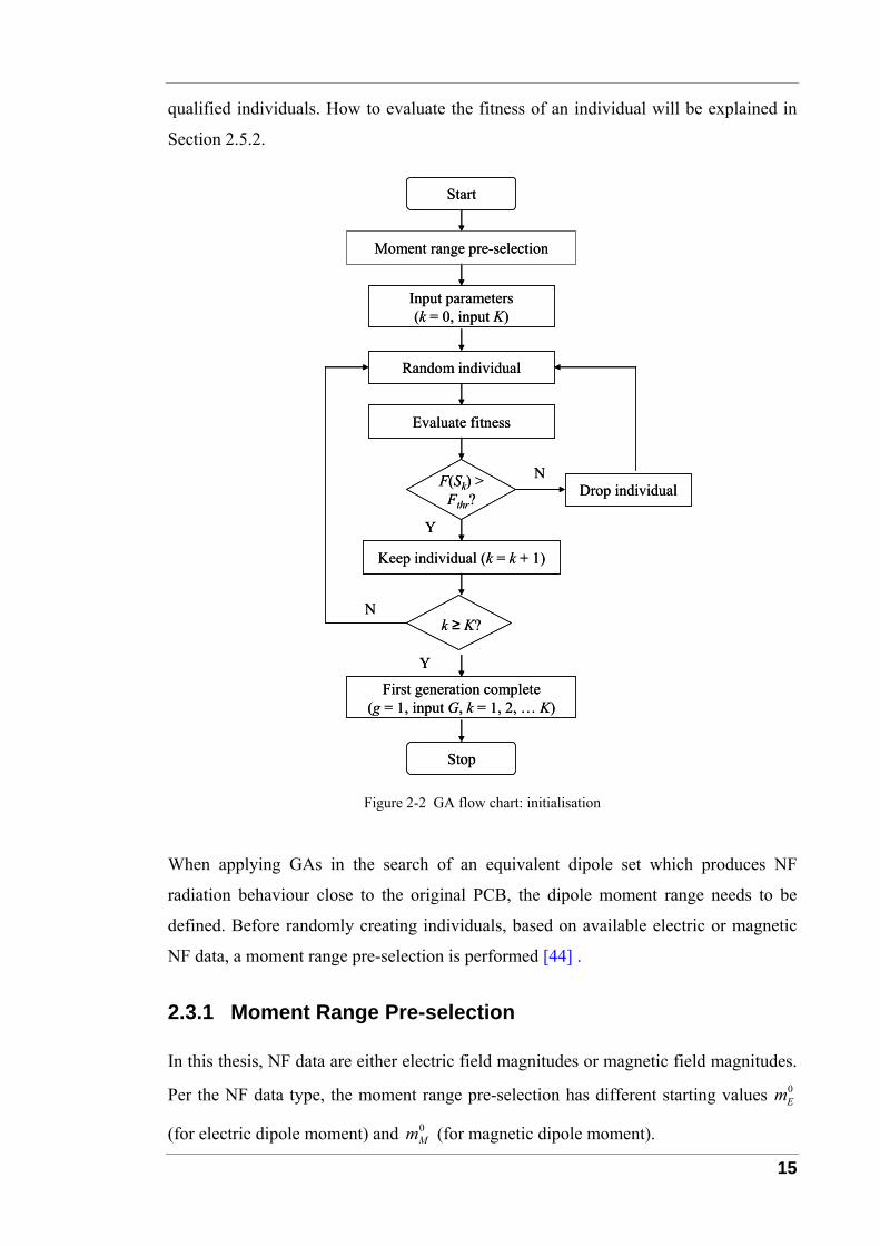
qualified individuals. How to evaluate the fitness of an individual will be explained in

Section 2.5.2.

Random individual

Evaluate fitness

F(Sk) >Fthr?

Keep individual (k = k + 1)

Drop individual

First generation complete(g = 1, input G, k = 1, 2, … K)

N

Y

Y

N

Start

Stop

Input parameters(k = 0, input K)

Moment range pre-selection

k ≥ K?

Random individual

Evaluate fitness

F(Sk) >Fthr?

Keep individual (k = k + 1)

Drop individual

First generation complete(g = 1, input G, k = 1, 2, … K)

N

Y

Y

N

Start

Stop

Input parameters(k = 0, input K)

Moment range pre-selection

k ≥ K?

Figure 2-2 GA flow chart: initialisation

When applying GAs in the search of an equivalent dipole set which produces NF

radiation behaviour close to the original PCB, the dipole moment range needs to be

defined. Before randomly creating individuals, based on available electric or magnetic

NF data, a moment range pre-selection is performed [44] .

2.3.1 Moment Range Pre-selection

In this thesis, NF data are either electric field magnitudes or magnetic field magnitudes.

Per the NF data type, the moment range pre-selection has different starting values 0Em

(for electric dipole moment) and 0Mm (for magnetic dipole moment).

16

The following is a step of initialising the above starting values when electric NF data

are available. In a spherical coordinate system (r – θ – φ) the electric NF, in a distance r

from the source, is approximately [5]

3 3

cos sin, , 0,2 4

E Er

m mE E Er rθ ϕθ θ

πεω πεω≈ ≈ = (2-3)

for an electric dipole, and

2

sin0, ,4

Mr

mE E Erθ ϕ

μω θπ

= = ≈ (2-4)

for a magnetic dipole, where Em and Mm mean the electric and magnetic dipole

moment, respectively. From all sample points the maximum value of the electric field,

Emax, is chosen, and starting values for electric and magnetic dipole moments are

initialised as

0 3max

20

max

4 ,

4 .

E

M

m E r

rm E

πεω

πμω

= ⋅

= ⋅ (2-5)

Similarly, when magnetic NF data are available, the step for initialising the starting

values is as follows. In a spherical coordinate system (r – θ – φ) the magnetic NF, in a

distance r from the source, is approximately [5]

2

sin , 0,4E

rmH H H

rϕ θθ

π≈ = = (2-6)

for an electric dipole, and

3 3

cos sin, , 0,2 4M M

rm mH H H

r rθ ϕθ θ

π π≈ ≈ = (2-7)

for a magnetic dipole, where Em and Mm mean the electric and magnetic dipole

moment, respectively. From all sample points the maximum value of the magnetic field,

Hmax, is chosen, and starting values for electric and magnetic dipole moments are

initialised as

0 2max

0 3max

4 ,

4 .E

M

m H r

m H r

π

π

= ⋅

= ⋅ (2-8)

The upper bound for the electric dipole moments is now varied systematically and set as

.15,14...,,14,15,20, −−=⋅= imm i

EiE (2-9)

17

The range for the magnetic dipole moments is kept at 0Mm . For each ,E im case a total of

100 individuals are randomly generated and the average fitness is evaluated (the

detailed calculation for fitness will be illustrated later in Section 2.5.2). In the next step

the range for the electric dipole moments is kept at 0Em and the magnetic moment range

is varied,

.15,14...,,14,15,20, −−=⋅= imm i

MiM (2-10)

Two sets of fitness values, ( )0, ,E i MF m m and ( )0

,,E M iF m m , are the outcome of this

procedure. The mean values of both sets are determined,

( )15

0, ,

1515

0, ,

15

1 , ,311 ( , ) .31

avg E E i Mi

avg M E M ii

F F m m

F F m m

=−

=−

=

=

∑

∑ (2-11)

From those moment ranges ,E im and ,M im which produce above-average results (fitness

values higher than ,avg EF and ,avg MF in (2-11), respectively) the largest range values are

picked up for the next pre-selection step:

1 0, , ,

1 0, , ,

sup , : ( , ) ,

sup , : ( , ) .

E E E E i E i M avg E

M M M M i E M i avg M

m m m m F m m F

m m m m F m m F

= = ≥

= = ≥ (2-12)

Typically, dipole moment ranges much smaller or much larger than 1Em or 1

Mm ,

respectively, result in poor fitness values, while moment ranges around the midfield

produce above-average fitness. Similar to (2-9) and (2-10) electric and magnetic

moment ranges are again varied systematically, but this time simultaneously,

1,

1,

2 , 11, 10, ..., 2, 3,

2 , 11, 10, ..., 2, 3.

iE i E

jM j M

m m i

m m j

= ⋅ = − −

= ⋅ = − − (2-13)

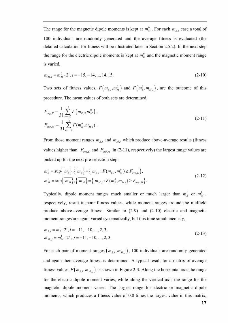
For each pair of moment ranges ( ), ,,E i M jm m , 100 individuals are randomly generated

and again their average fitness is determined. A typical result for a matrix of average

fitness values ( ), ,,E i M jF m m is shown in Figure 2-3. Along the horizontal axis the range

for the electric dipole moment varies, while along the vertical axis the range for the

magnetic dipole moment varies. The largest range for electric or magnetic dipole

moments, which produces a fitness value of 0.8 times the largest value in this matrix,

18

( )( ), ,0.8 max ,E i M jF m m⋅ , is then selected as the optimum value for the upper bound of

the dipole moment range.

In (2-3), (2-4), (2-6) and (2-7), it was assumed that observation points were in the NF.

For cases using FF data as the GA input (see Chapter 3), the above moment pre-

selection process is still valid. Although the initial values for the moment ranges in (2-5)

or (2-8) are very coarse, the further steps of (2-12) and (2-13) in a fine-tuning manner

would lead to appropriate values for the moment ranges.

2.3.2 Example

In the example shown in Figure 2-3 the maximum fitness value is 1.88, giving a

threshold of 1.50; from the fitness matrix it is found that for electric dipole moments

beyond the 12th column, and magnetic dipole moments above the 11th row fitness values

drop drastically. Dipole moment values corresponding to this column

( 12111 2 +−⋅= EoptE mm ) and this row ( 11111 2 +−⋅= M

optM mm ) would be chosen as the upper

bounds for electric and magnetic dipole moments in this instance.

Figure 2-3 Fitness matrix for fine-tuning the dipole moment ranges

19

Both electric and magnetic moment ranges should be selected appropriately in order to

get good fitness values. If dipole moment ranges are too small, corresponding to the left

hand side and lower edges of Figure 2-3, the fitness is close to 1. If dipole moments are

too large, corresponding to the right hand side and upper edges of Figure 2-3, the fitness

values drop close to zero. The optimum fitness values occur in the region in between.

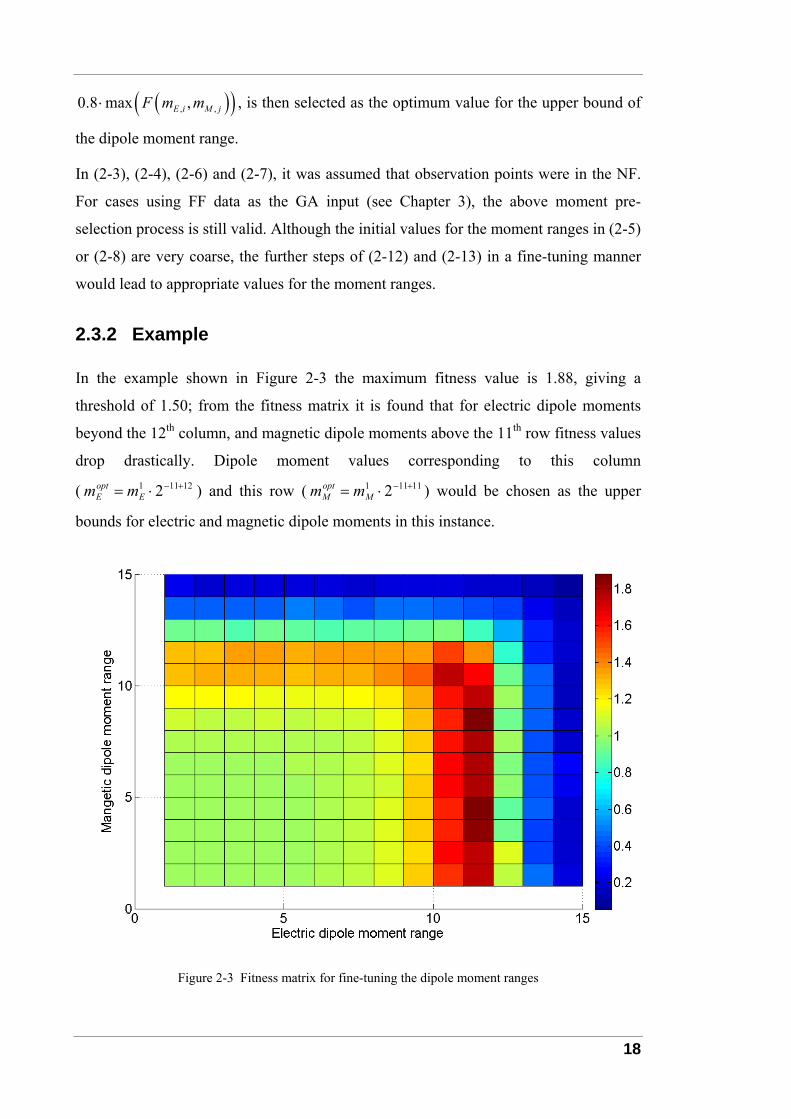
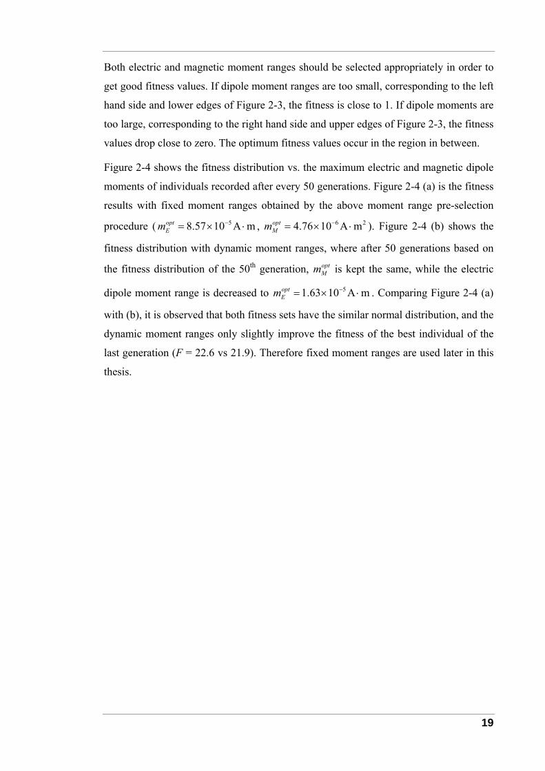
Figure 2-4 shows the fitness distribution vs. the maximum electric and magnetic dipole

moments of individuals recorded after every 50 generations. Figure 2-4 (a) is the fitness

results with fixed moment ranges obtained by the above moment range pre-selection

procedure ( 58.57 10 A moptEm −= × ⋅ , 6 24.76 10 A mopt

Mm −= × ⋅ ). Figure 2-4 (b) shows the

fitness distribution with dynamic moment ranges, where after 50 generations based on

the fitness distribution of the 50th generation, optMm is kept the same, while the electric

dipole moment range is decreased to 51.63 10 A moptEm −= × ⋅ . Comparing Figure 2-4 (a)

with (b), it is observed that both fitness sets have the similar normal distribution, and the

dynamic moment ranges only slightly improve the fitness of the best individual of the

last generation (F = 22.6 vs 21.9). Therefore fixed moment ranges are used later in this

thesis.

20

(a) Fixed moment ranges

(b) Dynamic moment ranges

Figure 2-4 Fitness distribution vs maximum electric and magnetic dipole moments

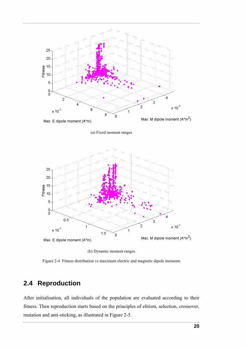
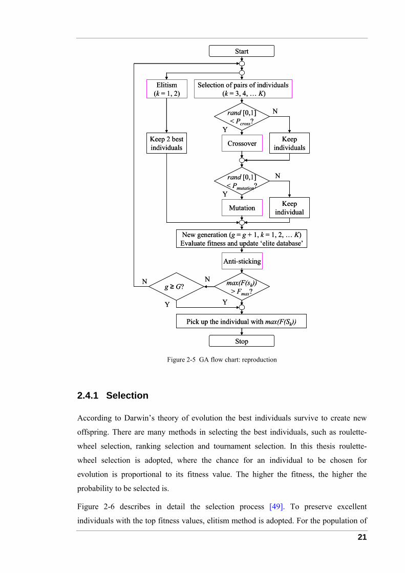
2.4 Reproduction

After initialisation, all individuals of the population are evaluated according to their

fitness. Then reproduction starts based on the principles of elitism, selection, crossover,

mutation and anti-sticking, as illustrated in Figure 2-5.

21

Elitism(k = 1, 2)

Crossover

Selection of pairs of individuals(k = 3, 4, … K)

rand [0,1]< Pcross?

New generation (g = g + 1, k = 1, 2, … K)Evaluate fitness and update ‘elite database’

Keep 2 bestindividuals

Stop

Pick up the individual with max(F(Sk))

Start

N

N

Y

Y

Keepindividuals

rand [0,1]< Pmutation?

Mutation

Y

N

Keepindividual

max(F(sk))> Fmax?

N

Y

Anti-sticking

g ≥ G?

Elitism(k = 1, 2)

Crossover

Selection of pairs of individuals(k = 3, 4, … K)

rand [0,1]< Pcross?

New generation (g = g + 1, k = 1, 2, … K)Evaluate fitness and update ‘elite database’

Keep 2 bestindividuals

Stop

Pick up the individual with max(F(Sk))

Start

N

N

Y

Y

Keepindividuals

rand [0,1]< Pmutation?

Mutation

Y

N

Keepindividual

max(F(sk))> Fmax?

N

Y

Anti-sticking

g ≥ G?

Figure 2-5 GA flow chart: reproduction

2.4.1 Selection

According to Darwin’s theory of evolution the best individuals survive to create new

offspring. There are many methods in selecting the best individuals, such as roulette-

wheel selection, ranking selection and tournament selection. In this thesis roulette-

wheel selection is adopted, where the chance for an individual to be chosen for

evolution is proportional to its fitness value. The higher the fitness, the higher the

probability to be selected is.

Figure 2-6 describes in detail the selection process [49]. To preserve excellent

individuals with the top fitness values, elitism method is adopted. For the population of

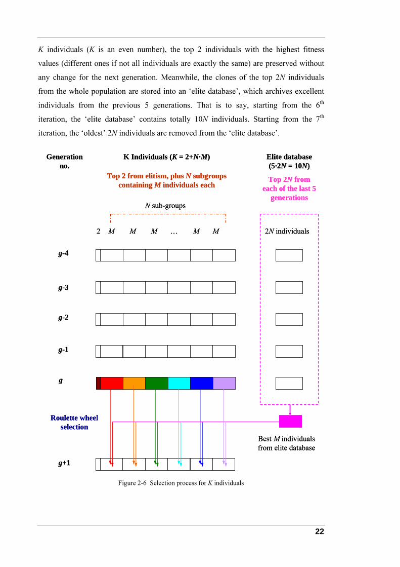
22

K individuals (K is an even number), the top 2 individuals with the highest fitness

values (different ones if not all individuals are exactly the same) are preserved without

any change for the next generation. Meanwhile, the clones of the top 2N individuals

from the whole population are stored into an ‘elite database’, which archives excellent

individuals from the previous 5 generations. That is to say, starting from the 6th

iteration, the ‘elite database’ contains totally 10N individuals. Starting from the 7th

iteration, the ‘oldest’ 2N individuals are removed from the ‘elite database’.

Roulette wheel selection

Elite database (5·2N = 10N)

Top 2N from each of the last 5

generations

Generation no.

g-4

K Individuals (K = 2+N·M)

Top 2 from elitism, plus N subgroups containing M individuals each

g-3

g-2

g-1

g

g+1

2 M M M … M M 2N individuals

N sub-groups

Best M individuals from elite database

Roulette wheel selection

Elite database (5·2N = 10N)

Top 2N from each of the last 5

generations

Generation no.

g-4

K Individuals (K = 2+N·M)

Top 2 from elitism, plus N subgroups containing M individuals each

g-3

g-2

g-1

g

g+1

2 M M M … M M 2N individuals

N sub-groups

Best M individuals from elite database

Figure 2-6 Selection process for K individuals

23

Apart from the 2 individuals kept by elitism, the remaining K-2 individuals are evenly

divided into N sub-groups, each of which contains M individuals. These subgroups

undergo the GA process in parallel. For the next generation of each sub-group, the two

best individuals from the previous generation become two parents (not necessarily in

one pair), other (M-2) parents are selected according to the roulette-wheel method from

a ‘selection pool’, which consists of the M individuals in the respective sub-group of the

previous generation, and also the best M individuals in the ‘elite database’.

For example, for a population of 62 individuals (K = 62), the 2 best individuals are

preserved by elitism, and the remaining 60 (K-2 = 60) are divided into 6 sub-groups (N

= 6) each of which contains 10 individuals (M = 10). The top two individuals of each

sub-group (2N = 12 in total) are archived in an ‘elite database’, eventually replacing the

‘oldest’ 12 individuals, if this database has been already filled (i.e. at least 6 generations

have passed so far). For each sub-group, the two best individuals from the previous

generation become two parents, other 8 parents (M-2 = 8) are selected from a ‘selection

pool’ of totally 20 individuals (2M = 20): the 10 individuals (M = 10) in this sub-group

from the previous generation, and the best 10 (M = 10) individuals in the ‘elite

database’.

Once the selection is done in parallel for all N subgroups, the GA goes to the crossover

step.

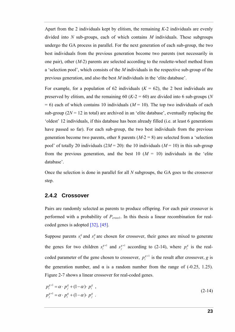
2.4.2 Crossover

Pairs are randomly selected as parents to produce offspring. For each pair crossover is

performed with a probability of Pcross1. In this thesis a linear recombination for real-

coded genes is adopted [32], [45].

Suppose parents gis and g

js are chosen for crossover, their genes are mixed to generate

the genes for two children 1gis + and 1g

js + according to (2-14), where gip is the real-

coded parameter of the gene chosen to crossover, 1gip + is the result after crossover, g is

the generation number, and α is a random number from the range of (-0.25, 1.25).

Figure 2-7 shows a linear crossover for real-coded genes.

1

1

(1 ) ,

(1 ) .

g g gi j i

g g gj i j

p p p

p p p

α α

α α

+

+

= ⋅ + − ⋅

= ⋅ + − ⋅ (2-14)

24

1gip +

1gjp +

gip

gjp

Before crossover

After crossover

α

α

1 α−

1 α−

1gip +

1gjp +

gip

gjp

Before crossover

After crossover

α

α

1 α−

1 α−

Figure 2-7 Linear crossover for real-coded genes

LB and UB are lower and upper domain bounds of the variable pi. If 1gip + is out of range,

then the parameter 1gip + is adjusted to 1g

ip + :

1 1

1

( ),

,

g gi i

gi

p p k UB LB

p LBk floorUB LB

+ +

+

= − −

⎛ ⎞−= ⎜ ⎟−⎝ ⎠

(2-15)

where the function floor(x) rounds the element of x to the nearest integer less than or

equal to x.

Individual pairs with the probability of crossover Pcross1 are chosen for crossover, where

the genes of these pairs perform crossover with the probability of Pcross2 [45]. So the

total probability for a particular pair of genes to crossover is

1 2 .cross cross crossP P P= ⋅ (2-16)

In this thesis, Pcross2 = 0.9 is used, and the value for Pcross1 is dependent on the ‘sticking’

status during the progress, as described later in Section 2.4.3.

Since the moment ranges for electric and magnetic dipoles are usually different,

particular attention should be paid to eliminate the chance of crossover between electric

and magnetic dipoles. After the selection based on the fitness values, the genes of

individuals are re-arranged according to the dipole type. Between the same type of

dipoles, crossover for moment magnitude mq is done according to (2-14); while for

different type Kq of dipoles, Kq and mq are simultaneously swapped with each other.

25

2.4.3 Mutation

Mutation introduces genetic material that is not present in the current population, to

ensure that overly aggressive selection does not result in premature convergence to a

sub-optimum solution. The individuals of the new generation, except the two

individuals preserved by elitism, are subject to mutation with a probability of Pmutate.

GAs have sometimes the tendency to get stuck at local optima. An indication for this

phenomenon is that the two fittest individuals are the same as in the previous

generation. If a new generation has the same two best fitness values as the previous one,

action should be taken to make it more likely to introduce new genetic material, such as

increasing the probability of mutation, manipulating the mutation step and replacing

some individuals.

Mutation is a core process of GAs. Whether mutation operators are well defined for

anti-sticking, decides whether GAs can successfully find the optimum solution. In this

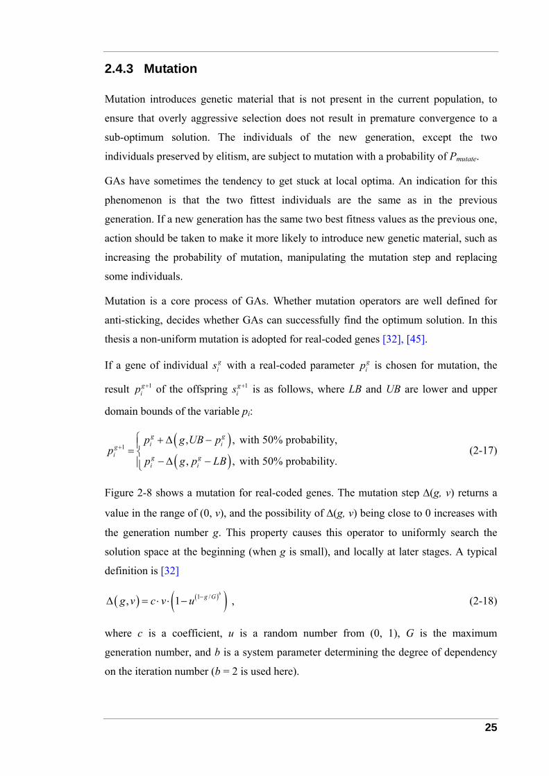
thesis a non-uniform mutation is adopted for real-coded genes [32], [45].

If a gene of individual gis with a real-coded parameter g

ip is chosen for mutation, the

result 1gip + of the offspring 1g

is + is as follows, where LB and UB are lower and upper

domain bounds of the variable pi:

( )( )

1, , with 50% probability,

, , with 50% probability.

g gi ig

i g gi i

p g UB pp

p g p LB+

⎧ + Δ −⎪= ⎨− Δ −⎪⎩

(2-17)

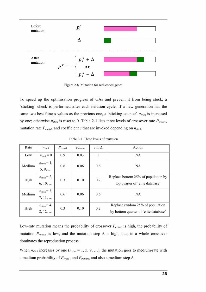
Figure 2-8 shows a mutation for real-coded genes. The mutation step Δ(g, v) returns a

value in the range of (0, v), and the possibility of Δ(g, v) being close to 0 increases with

the generation number g. This property causes this operator to uniformly search the

solution space at the beginning (when g is small), and locally at later stages. A typical

definition is [32]

( ) ( )( )1 /, 1 ,bg Gg v c v u −Δ = ⋅ ⋅ − (2-18)

where c is a coefficient, u is a random number from (0, 1), G is the maximum

generation number, and b is a system parameter determining the degree of dependency

on the iteration number (b = 2 is used here).

26

gipBefore

mutation

After mutation

1 o r

gi

gi

gi

pp

p

+

⎧ + Δ⎪= ⎨⎪ − Δ⎩

Δ

gipBefore

mutation

After mutation

1 o r

gi

gi

gi

pp

p

+

⎧ + Δ⎪= ⎨⎪ − Δ⎩

Δ

Figure 2-8 Mutation for real-coded genes

To speed up the optimisation progress of GAs and prevent it from being stuck, a

‘sticking’ check is performed after each iteration cycle. If a new generation has the

same two best fitness values as the previous one, a ‘sticking counter’ nstick is increased

by one; otherwise nstick is reset to 0. Table 2-1 lists three levels of crossover rate Pcross1,

mutation rate Pmutate and coefficient c that are invoked depending on nstick.

Table 2-1 Three levels of mutation

Rate nstick Pcross1 Pmutate c in Δ Action

Low nstick = 0 0.9 0.03 1 NA

Medium nstick = 1,

5, 9, … 0.6 0.06 0.6 NA

High nstick = 2,

6, 10, … 0.3 0.10 0.2

Replace bottom 25% of population by

top quarter of ‘elite database’

Medium nstick = 3,

7, 11, … 0.6 0.06 0.6 NA

High nstick = 4,

8, 12, … 0.3 0.10 0.2

Replace random 25% of population

by bottom quarter of ‘elite database’

Low-rate mutation means the probability of crossover Pcross1 is high, the probability of

mutation Pmutate is low, and the mutation step Δ is high, thus in a whole crossover

dominates the reproduction process.

When nstick increases by one (nstick = 1, 5, 9, …), the mutation goes to medium-rate with

a medium probability of Pcross1 and Pmutate, and also a medium step Δ.

27

After the next iteration, if nstick again increases by one (nstick = 2, 6, 10, …), the quarter of

the population with the worst fitness values is replaced by the top quarter of the

archived ‘elite database’. A low Pcross1 and a high Pmutate are used with a low Δ.

These two iterations with higher rate mutation more or less realise a local searching

around the best individuals. If the sticking problem is resolved after this measure, nstick

is reset to 0; otherwise, nstick is increased (nstick = 3, 7, 11, …), and another iteration with

a medium-rate mutation is performed. If there is still no improvement in the fitness of

the two best individuals (now nstick = 4, 8, 12, …), a high-rate mutation is conducted,

and a random quarter of the population is replaced by the bottom quarter of the archived

‘elite database’. After that if nstick still increases, stages with a medium-rate mutation, a

high-rate mutation and partial replacement are alternated.

Similar to crossover, Kq and mq are required to mutate together. The mutation occurs

with the probability of Pmutate. With a 50% probability, Kq is kept the same as before,

while the mq is mutated according to (2-18); with another 50% probability, Kq is

changed and the mq is mutated based on the magnitude randomly selected from the

separate databases which hold all electric and magnetic dipole mq information of the

current generation.

The reproduction process is repeated until the best fitness value is better than the target

Fmax, or for a maximum of G generations, whatever happens first (see Figure 2-5).

2.5 Evaluation of Genetic Algorithms

Generated by selecting the best individuals from the current generation and mating them,

the next generation contains a higher proportion of the characteristics possessed by the

better fit members of the previous one. In this way, over generations, good

characteristics are spread throughout the population. If a GA is well designed, the

population will converge to an optimum solution to the problem. This section serves to

evaluate the performance of GAs in the NF-FF conversion.

2.5.1 Source Identification

This section is to check whether GAs can identify an original radiator. For comparison

with previous work, the four original dipoles (t1, t2, t3, t4) at 30 MHz in free space listed

in Table I of [12] are selected as a known source. 124 sample points are chosen on a

28

sphere of 0.6 m radius, and their electric NF data (peak values for Ex, Ey and Ez) are

calculated based on the approximated field equations for infinitesimal dipoles shown in

Appendix C.

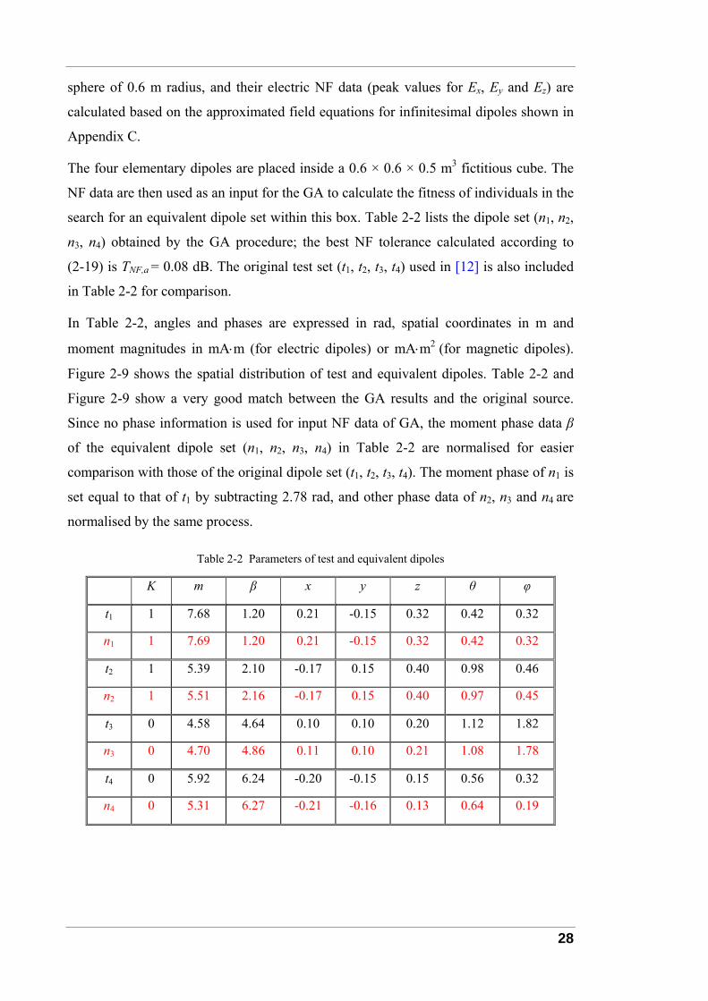
The four elementary dipoles are placed inside a 0.6 × 0.6 × 0.5 m3 fictitious cube. The

NF data are then used as an input for the GA to calculate the fitness of individuals in the

search for an equivalent dipole set within this box. Table 2-2 lists the dipole set (n1, n2,

n3, n4) obtained by the GA procedure; the best NF tolerance calculated according to

(2-19) is TNF,a = 0.08 dB. The original test set (t1, t2, t3, t4) used in [12] is also included

in Table 2-2 for comparison.

In Table 2-2, angles and phases are expressed in rad, spatial coordinates in m and

moment magnitudes in mA⋅m (for electric dipoles) or mA⋅m2 (for magnetic dipoles).

Figure 2-9 shows the spatial distribution of test and equivalent dipoles. Table 2-2 and

Figure 2-9 show a very good match between the GA results and the original source.

Since no phase information is used for input NF data of GA, the moment phase data β

of the equivalent dipole set (n1, n2, n3, n4) in Table 2-2 are normalised for easier

comparison with those of the original dipole set (t1, t2, t3, t4). The moment phase of n1 is

set equal to that of t1 by subtracting 2.78 rad, and other phase data of n2, n3 and n4 are

normalised by the same process.

Table 2-2 Parameters of test and equivalent dipoles

K m β x y z θ φ

t1 1 7.68 1.20 0.21 -0.15 0.32 0.42 0.32

n1 1 7.69 1.20 0.21 -0.15 0.32 0.42 0.32

t2 1 5.39 2.10 -0.17 0.15 0.40 0.98 0.46

n2 1 5.51 2.16 -0.17 0.15 0.40 0.97 0.45

t3 0 4.58 4.64 0.10 0.10 0.20 1.12 1.82

n3 0 4.70 4.86 0.11 0.10 0.21 1.08 1.78

t4 0 5.92 6.24 -0.20 -0.15 0.15 0.56 0.32

n4 0 5.31 6.27 -0.21 -0.16 0.13 0.64 0.19

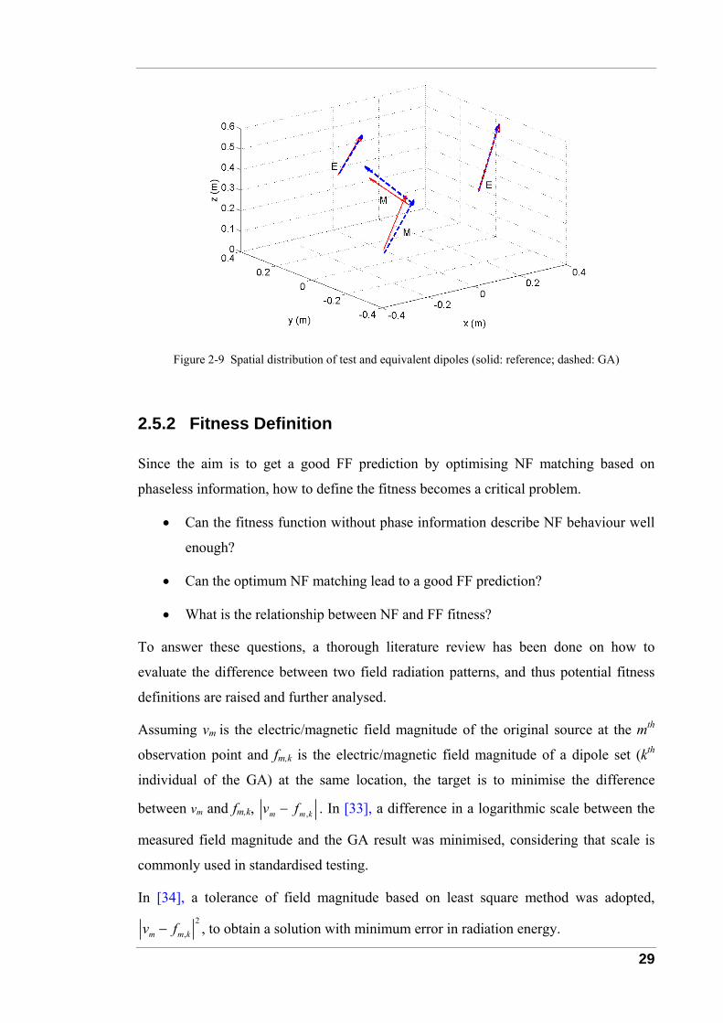
29

Figure 2-9 Spatial distribution of test and equivalent dipoles (solid: reference; dashed: GA)

2.5.2 Fitness Definition

Since the aim is to get a good FF prediction by optimising NF matching based on

phaseless information, how to define the fitness becomes a critical problem.

• Can the fitness function without phase information describe NF behaviour well

enough?

• Can the optimum NF matching lead to a good FF prediction?

• What is the relationship between NF and FF fitness?

To answer these questions, a thorough literature review has been done on how to

evaluate the difference between two field radiation patterns, and thus potential fitness

definitions are raised and further analysed.

Assuming vm is the electric/magnetic field magnitude of the original source at the mth

observation point and fm,k is the electric/magnetic field magnitude of a dipole set (kth

individual of the GA) at the same location, the target is to minimise the difference

between vm and fm,k, ,m m kv f− . In [33], a difference in a logarithmic scale between the

measured field magnitude and the GA result was minimised, considering that scale is

commonly used in standardised testing.

In [34], a tolerance of field magnitude based on least square method was adopted, 2

,m m kv f− , to obtain a solution with minimum error in radiation energy.

30

In [24], a quadratic inverse approach was raised for calculating least square of field

intensity tolerance, 22 2

,m m kv f− . It was stated that choice of field intensities gave a

simpler nonlinearity than that of magnitudes, and thus got rid of possible local minima

problems in the function defining the solution.

In [51], a multi-objective algorithm was introduced for evolutionary optimisation. An

easy way to realise it is to combine different objectives into one fitness function (e.g. by

a linear operation when they share the same measurement unit).

2.5.2.1 Near Field Tolerance

To compare the above considerations in the literature and find an optimum fitness

definition, eight expressions for tolerance between reference values and the

approximation are evaluated:

( ), ,1

20 lg lg ;M

NF a k m m km

T s v fM =

= ⋅ −∑ (2-19)

( ) ,,

1

1 ;M

m m kNF b k

m m

v fT s

M v=

−= ⋅∑ (2-20)

( )( )2

,1

,2

1

;

M

m m km

NF c k M

mm

v fT s

v

=

=

−=

∑

∑ (2-21)

( )2 2

,, 2

1

1 ;M

m m kNF d k

m m

v fT s

M v=

−= ⋅∑ (2-22)

( )( )22 2

,1

,4

1

;

M

m m km

NF e k M

mm

v fT s

v

=

=

−=

∑

∑ (2-23)

( ) ( ) ( ) ( ), , ,1 , 0.25 ;NF f k NF b k NF c kT s T s T sα α α= − ⋅ + ⋅ = (2-24)

( ) ( ) ( ) ( ), , ,1 , 0.5 ;NF g k NF b k NF c kT s T s T sα α α= − ⋅ + ⋅ = (2-25)

( ) ( ) ( ) ( ), , ,1 , 0.75 .NF h k NF b k NF c kT s T s T sα α α= − ⋅ + ⋅ = (2-26)

TNF,a considers an average field strength difference of all test points in a logarithmic

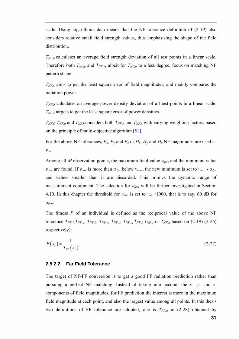
31

scale. Using logarithmic data means that the NF tolerance definition of (2-19) also

considers relative small field strength values, thus emphasising the shape of the field

distribution.

TNF,b calculates an average field strength deviation of all test points in a linear scale.

Therefore both TNF,a and TNF,b, albeit for TNF,b to a less degree, focus on matching NF

pattern shape.

TNF,c aims to get the least square error of field magnitudes, and mainly compares the

radiation power.

TNF,d calculates an average power density deviation of all test points in a linear scale.

TNF,e targets to get the least square error of power densities.

TNF,f, TNF,g and TNF,h considers both TNF,b and TNF,c with varying weighting factors, based

on the principle of multi-objective algorithm [51].

For the above NF tolerances, Ex, Ey and Ez or Hx, Hy and Hz NF magnitudes are used as

vm.

Among all M observation points, the maximum field value vmax and the minimum value

vmin are found. If vmin is more than adyn below vmax, the new minimum is set to vmax - adyn

and values smaller than it are discarded. This mimics the dynamic range of

measurement equipment. The selection for adyn will be further investigated in Section

4.10. In this chapter the threshold for vmin is set to vmax/1000, that is to say, 60 dB for

adyn.

The fitness F of an individual is defined as the reciprocal value of the above NF

tolerance TNF (TNF,a, TNF,b, TNF,c, TNF,d, TNF,e, TNF,f, TNF,g or TNF,h based on (2-19)-(2-26)

respectively):

( ) ( )1 .k

NF k

F sT s

= (2-27)

2.5.2.2 Far Field Tolerance

The target of NF-FF conversion is to get a good FF radiation prediction rather than

pursuing a perfect NF matching. Instead of taking into account the x-, y- and z-

components of field magnitudes, for FF prediction the interest is more in the maximum

field magnitude at each point, and also the largest value among all points. In this thesis

two definitions of FF tolerance are adopted, one is TFF,a in (2-28) obtained by

32

calculating the deviation of maximum field magnitudes at M points, where

2 2 2m x y zv E E E= + + or 2 2 2

m x y zv H H H= + + ; the other is TFF,max shown in (2-29),

where vmax and fk,max mean the largest value of maximum field magnitude among all M

points, obtained from reference data and GA results respectively.

( ), ,1

20 lg lg ;M

FF a k m m km

T s v fM =

= ⋅ −∑ (2-28)

( ),max max ,max20 lg lg .FF k kT s v f= ⋅ − (2-29)

For FF tolerance TFF calculation, the total electric field magnitude E is calculated

according to Appendix C and used as reference data without any filtering.

2.5.2.3 Near Field-Far Field Tolerance Correlation

A fundamental problem in the case of NF-FF conversion is that the actual FF tolerance

can not be determined. Ultimately it is important to achieve a good agreement between

the GA dipole model and the PCB for the FF. Therefore the definition of NF matching

should be well related to the final FF matching. In [46], the fitness definition of NF

matching and FF prediction was addressed, and the correlation between NF and FF

fitness was analysed.

As a common measure of the linear relationship between the paired values of two

random variables X and Y, the correlation coefficient Corr, is defined as

( )( )( )( ) ( )2 2

, ,x x y y

Corr X Yx x y y

− −=

− −

∑∑

(2-30)

where x and y means average of X and Y, respectively.

It has to be established that a good approximation for the NF does indeed mean a good

approximation for the FF. Therefore the correlation coefficient Corr(X,Y) in (2-30) is

considered, where the probability distribution X represents the NF tolerance according

to (2-19) – (2-26) for all individuals respectively, and Y represents the FF tolerance

according to (2-28) or (2-29).

A correlation coefficient close to 1 indicates, that a good NF approximation also means

a good FF approximation.

To get an impression of the correlation between NF and FF tolerances, the equivalent

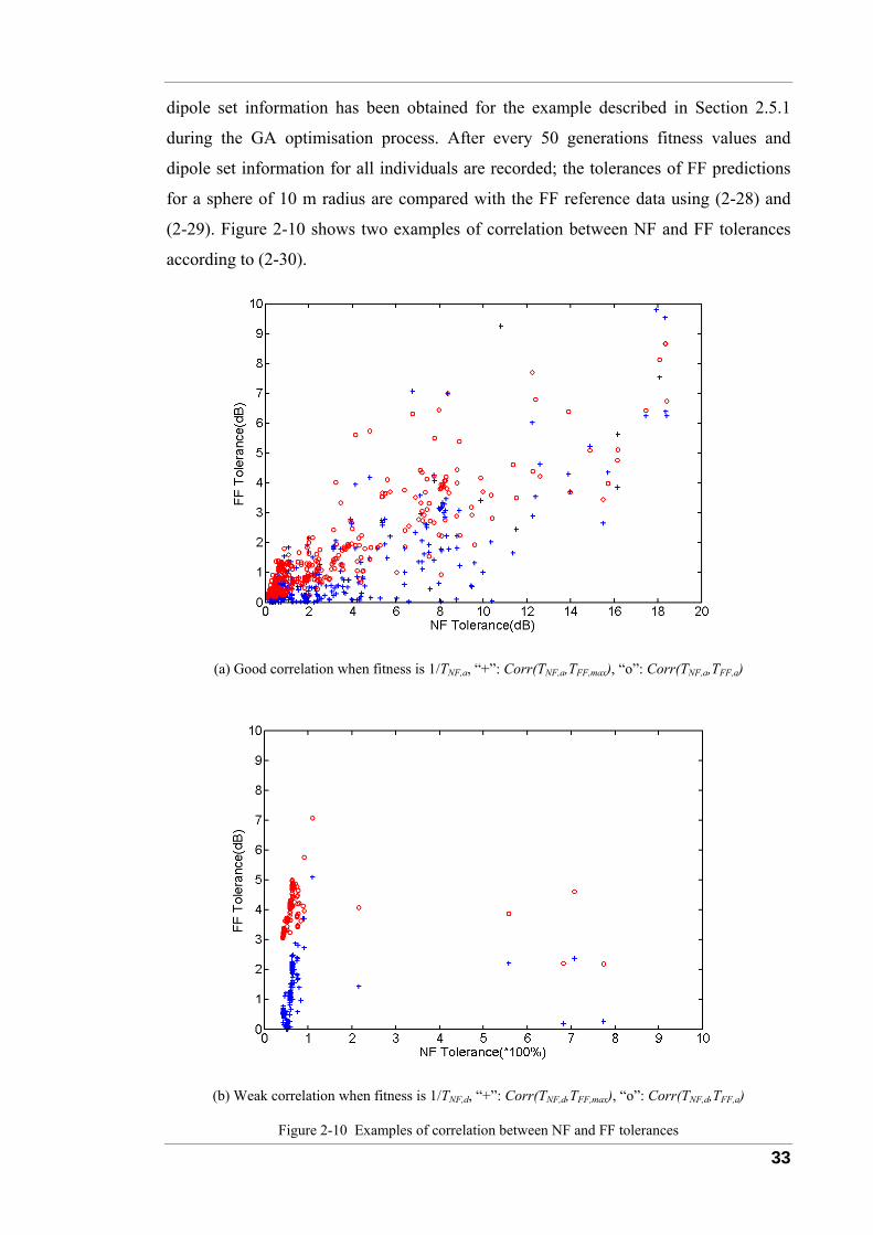
33

dipole set information has been obtained for the example described in Section 2.5.1

during the GA optimisation process. After every 50 generations fitness values and

dipole set information for all individuals are recorded; the tolerances of FF predictions

for a sphere of 10 m radius are compared with the FF reference data using (2-28) and

(2-29). Figure 2-10 shows two examples of correlation between NF and FF tolerances

according to (2-30).

(a) Good correlation when fitness is 1/TNF,a, “+”: Corr(TNF,a,TFF,max), “o”: Corr(TNF,a,TFF,a)

(b) Weak correlation when fitness is 1/TNF,d, “+”: Corr(TNF,d,TFF,max), “o”: Corr(TNF,d,TFF,a)

Figure 2-10 Examples of correlation between NF and FF tolerances

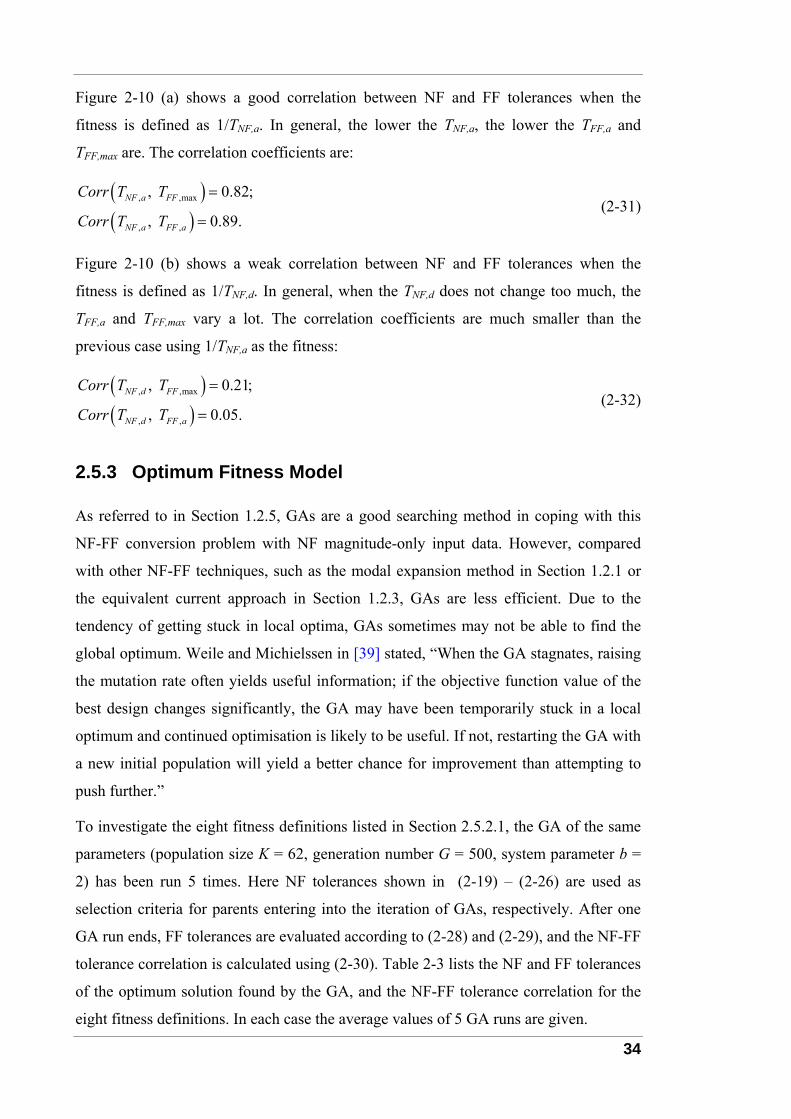
34

Figure 2-10 (a) shows a good correlation between NF and FF tolerances when the

fitness is defined as 1/TNF,a. In general, the lower the TNF,a, the lower the TFF,a and

TFF,max are. The correlation coefficients are:

( )( )

, ,max

, ,

, 0.82;

, 0.89.NF a FF

NF a FF a

Corr T T

Corr T T

=

= (2-31)

Figure 2-10 (b) shows a weak correlation between NF and FF tolerances when the

fitness is defined as 1/TNF,d. In general, when the TNF,d does not change too much, the

TFF,a and TFF,max vary a lot. The correlation coefficients are much smaller than the

previous case using 1/TNF,a as the fitness:

( )( )

, ,max

, ,

, 0.21;

, 0.05.NF d FF

NF d FF a

Corr T T

Corr T T

=

= (2-32)

2.5.3 Optimum Fitness Model

As referred to in Section 1.2.5, GAs are a good searching method in coping with this

NF-FF conversion problem with NF magnitude-only input data. However, compared

with other NF-FF techniques, such as the modal expansion method in Section 1.2.1 or

the equivalent current approach in Section 1.2.3, GAs are less efficient. Due to the

tendency of getting stuck in local optima, GAs sometimes may not be able to find the

global optimum. Weile and Michielssen in [39] stated, “When the GA stagnates, raising

the mutation rate often yields useful information; if the objective function value of the

best design changes significantly, the GA may have been temporarily stuck in a local

optimum and continued optimisation is likely to be useful. If not, restarting the GA with

a new initial population will yield a better chance for improvement than attempting to

push further.”

To investigate the eight fitness definitions listed in Section 2.5.2.1, the GA of the same

parameters (population size K = 62, generation number G = 500, system parameter b =

2) has been run 5 times. Here NF tolerances shown in (2-19) – (2-26) are used as

selection criteria for parents entering into the iteration of GAs, respectively. After one

GA run ends, FF tolerances are evaluated according to (2-28) and (2-29), and the NF-FF

tolerance correlation is calculated using (2-30). Table 2-3 lists the NF and FF tolerances

of the optimum solution found by the GA, and the NF-FF tolerance correlation for the

eight fitness definitions. In each case the average values of 5 GA runs are given.

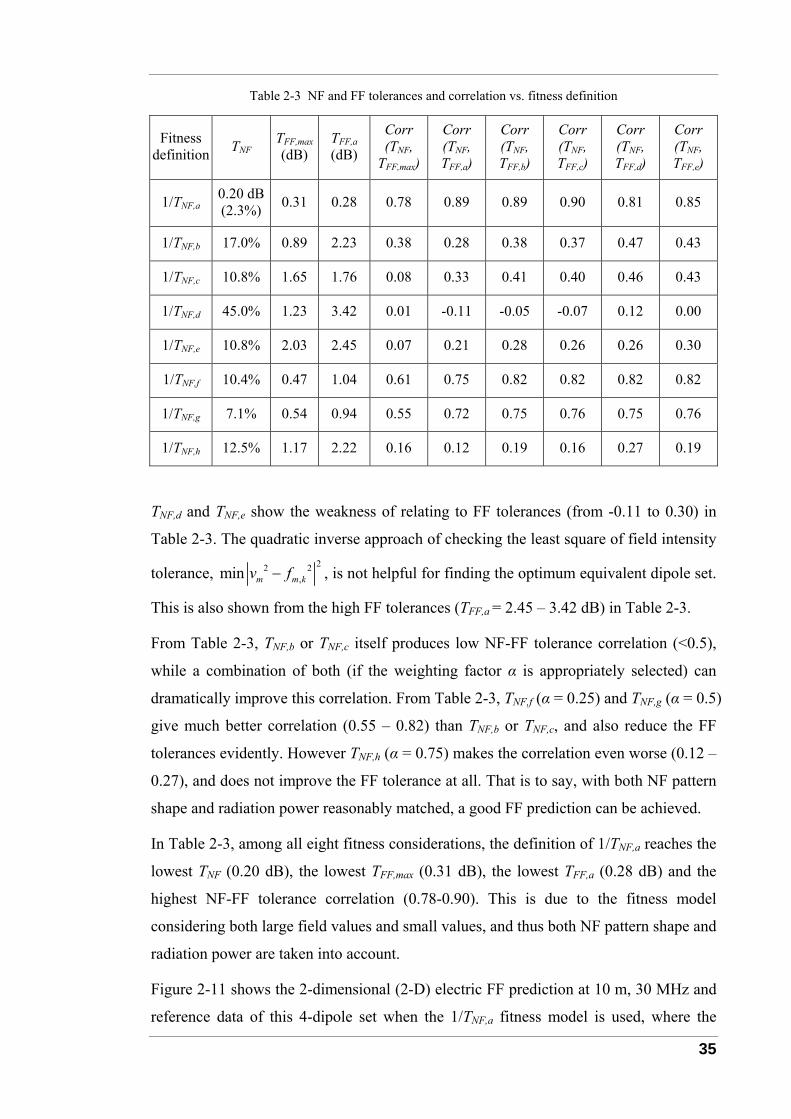
35

Table 2-3 NF and FF tolerances and correlation vs. fitness definition

Fitness definition TNF TFF,max

(dB) TFF,a (dB)

Corr (TNF,

TFF,max)

Corr (TNF, TFF,a)

Corr (TNF, TFF,b)

Corr (TNF, TFF,c)

Corr (TNF, TFF,d)

Corr (TNF, TFF,e)

1/TNF,a 0.20 dB (2.3%) 0.31 0.28 0.78 0.89 0.89 0.90 0.81 0.85

1/TNF,b 17.0% 0.89 2.23 0.38 0.28 0.38 0.37 0.47 0.43

1/TNF,c 10.8% 1.65 1.76 0.08 0.33 0.41 0.40 0.46 0.43

1/TNF,d 45.0% 1.23 3.42 0.01 -0.11 -0.05 -0.07 0.12 0.00

1/TNF,e 10.8% 2.03 2.45 0.07 0.21 0.28 0.26 0.26 0.30

1/TNF,f 10.4% 0.47 1.04 0.61 0.75 0.82 0.82 0.82 0.82

1/TNF,g 7.1% 0.54 0.94 0.55 0.72 0.75 0.76 0.75 0.76

1/TNF,h 12.5% 1.17 2.22 0.16 0.12 0.19 0.16 0.27 0.19

TNF,d and TNF,e show the weakness of relating to FF tolerances (from -0.11 to 0.30) in

Table 2-3. The quadratic inverse approach of checking the least square of field intensity

tolerance, 22 2

,min m m kv f− , is not helpful for finding the optimum equivalent dipole set.

This is also shown from the high FF tolerances (TFF,a = 2.45 – 3.42 dB) in Table 2-3.

From Table 2-3, TNF,b or TNF,c itself produces low NF-FF tolerance correlation (<0.5),

while a combination of both (if the weighting factor α is appropriately selected) can

dramatically improve this correlation. From Table 2-3, TNF,f (α = 0.25) and TNF,g (α = 0.5)

give much better correlation (0.55 – 0.82) than TNF,b or TNF,c, and also reduce the FF

tolerances evidently. However TNF,h (α = 0.75) makes the correlation even worse (0.12 –

0.27), and does not improve the FF tolerance at all. That is to say, with both NF pattern

shape and radiation power reasonably matched, a good FF prediction can be achieved.

In Table 2-3, among all eight fitness considerations, the definition of 1/TNF,a reaches the

lowest TNF (0.20 dB), the lowest TFF,max (0.31 dB), the lowest TFF,a (0.28 dB) and the

highest NF-FF tolerance correlation (0.78-0.90). This is due to the fitness model

considering both large field values and small values, and thus both NF pattern shape and

radiation power are taken into account.

Figure 2-11 shows the 2-dimensional (2-D) electric FF prediction at 10 m, 30 MHz and

reference data of this 4-dipole set when the 1/TNF,a fitness model is used, where the

36

mapping of the GA results has a good agreement with the reference FF pattern. The

later sections of this thesis will keep using the 1/TNF,a fitness model.

(a) Reference pattern (b) GA of 1/TNF,a fitness model

Figure 2-11 Mapping of electric FF patterns (field strength in dBmV/m)

2.5.4 Evolution Process of Genes

To illustrate how the GA works in its search for the equivalent dipole set, the relative

information of evolution is plotted.

As mentioned in Section 2.5.2.3, after every 50 generations fitness values and dipole set

information for all individuals are stored. Figure 2-12 shows the evolution of some

genes (dipole moment magnitude, location and orientation) together with NF and FF

tolerances, when the optimum 1/TNF,a fitness model is used. While Figure 2-9 shows

only the best individual at the end of the process, Figure 2-12 (a) shows all individuals

after 1, 50, 250, and 450 generations. Figure 2-12 (b) shows basically the information as

already depicted in Figure 2-10. While Figure 2-10 contains the information for all

individuals, after 1, 50, 100, …, 500 generations each picture in Figure 2-12 contains

only data for K individuals of the respective generation (K = 62 in this case).

At the 1st generation, dipole set information is randomly initialised, and thus the

tolerances vary widely (6 – 20 dB for TNF,a, and 1 – 10 dB for TFF,a). The tolerances

could be reduced by a more sophisticated initialisation process, but that would also

increase the computational burden for this stage.

After 50 iterations, the GA has already demonstrated its ability to tackle this

optimisation problem, and the dipole locations are closer to the reference data. Also the

tolerances have sharply decreased (2 – 10 dB for TNF,a, and 1 – 4 dB for TFF,a).

37

(a) Genes (b) NF-FF tolerances

Figure 2-12 Evolution in GA: “+”: Corr(TNF,a,TFF,max), “o”: Corr(TNF,a,TFF,a)

1st: Randomly generated individuals in the 1st generation vary widely;

50th: The really bad ones are quickly eliminated and some individuals with much better genes evolve;

250th: Most of the individuals have very good characteristics, but there are still occasional outlaws;

450th: Almost all of the individuals have quite good characteristics.

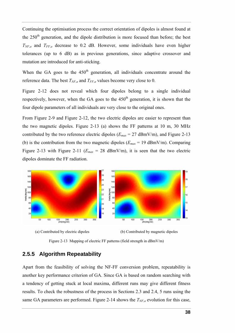
38

Continuing the optimisation process the correct orientation of dipoles is almost found at

the 250th generation, and the dipole distribution is more focused than before; the best

TNF,a and TFF,a decrease to 0.2 dB. However, some individuals have even higher

tolerances (up to 6 dB) as in previous generations, since adaptive crossover and

mutation are introduced for anti-sticking.

When the GA goes to the 450th generation, all individuals concentrate around the

reference data. The best TNF,a and TFF,a values become very close to 0.

Figure 2-12 does not reveal which four dipoles belong to a single individual

respectively, however, when the GA goes to the 450th generation, it is shown that the

four dipole parameters of all individuals are very close to the original ones.

From Figure 2-9 and Figure 2-12, the two electric dipoles are easier to represent than

the two magnetic dipoles. Figure 2-13 (a) shows the FF patterns at 10 m, 30 MHz

contributed by the two reference electric dipoles (Emax = 27 dBmV/m), and Figure 2-13

(b) is the contribution from the two magnetic dipoles (Emax = 19 dBmV/m). Comparing

Figure 2-13 with Figure 2-11 (Emax = 28 dBmV/m), it is seen that the two electric

dipoles dominate the FF radiation.

(a) Contributed by electric dipoles (b) Contributed by magnetic dipoles

Figure 2-13 Mapping of electric FF patterns (field strength in dBmV/m)

2.5.5 Algorithm Repeatability

Apart from the feasibility of solving the NF-FF conversion problem, repeatability is

another key performance criterion of GA. Since GA is based on random searching with

a tendency of getting stuck at local maxima, different runs may give different fitness

results. To check the robustness of the process in Sections 2.3 and 2.4, 5 runs using the

same GA parameters are performed. Figure 2-14 shows the TNF,a evolution for this case,

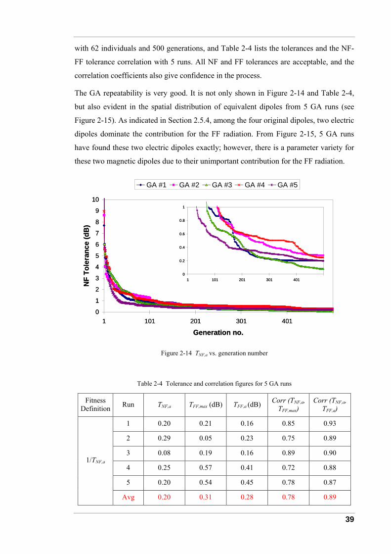
39

with 62 individuals and 500 generations, and Table 2-4 lists the tolerances and the NF-

FF tolerance correlation with 5 runs. All NF and FF tolerances are acceptable, and the

correlation coefficients also give confidence in the process.

The GA repeatability is very good. It is not only shown in Figure 2-14 and Table 2-4,

but also evident in the spatial distribution of equivalent dipoles from 5 GA runs (see

Figure 2-15). As indicated in Section 2.5.4, among the four original dipoles, two electric

dipoles dominate the contribution for the FF radiation. From Figure 2-15, 5 GA runs

have found these two electric dipoles exactly; however, there is a parameter variety for

these two magnetic dipoles due to their unimportant contribution for the FF radiation.

0

1

2

3

4

5

6

7

8

9

10

1 101 201 301 401

Generation no.

NF

Tole

ranc

e (d

B)

GA #1 GA #2 GA #3 GA #4 GA #5

0

0.2

0.4

0.6

0.8

1

1 101 201 301 401

0

1

2

3

4

5

6

7

8

9

10

1 101 201 301 401

Generation no.

NF

Tole

ranc

e (d

B)

GA #1 GA #2 GA #3 GA #4 GA #5

0

0.2

0.4

0.6

0.8

1

1 101 201 301 401

Figure 2-14 TNF,a vs. generation number

Table 2-4 Tolerance and correlation figures for 5 GA runs

Fitness Definition Run TNF,a TFF,max (dB) TFF,a (dB) Corr (TNF,a,

TFF,max) Corr (TNF,a,

TFF,a)

1 0.20 0.21 0.16 0.85 0.93

2 0.29 0.05 0.23 0.75 0.89

3 0.08 0.19 0.16 0.89 0.90

4 0.25 0.57 0.41 0.72 0.88

5 0.20 0.54 0.45 0.78 0.87

1/TNF,a

Avg 0.20 0.31 0.28 0.78 0.89

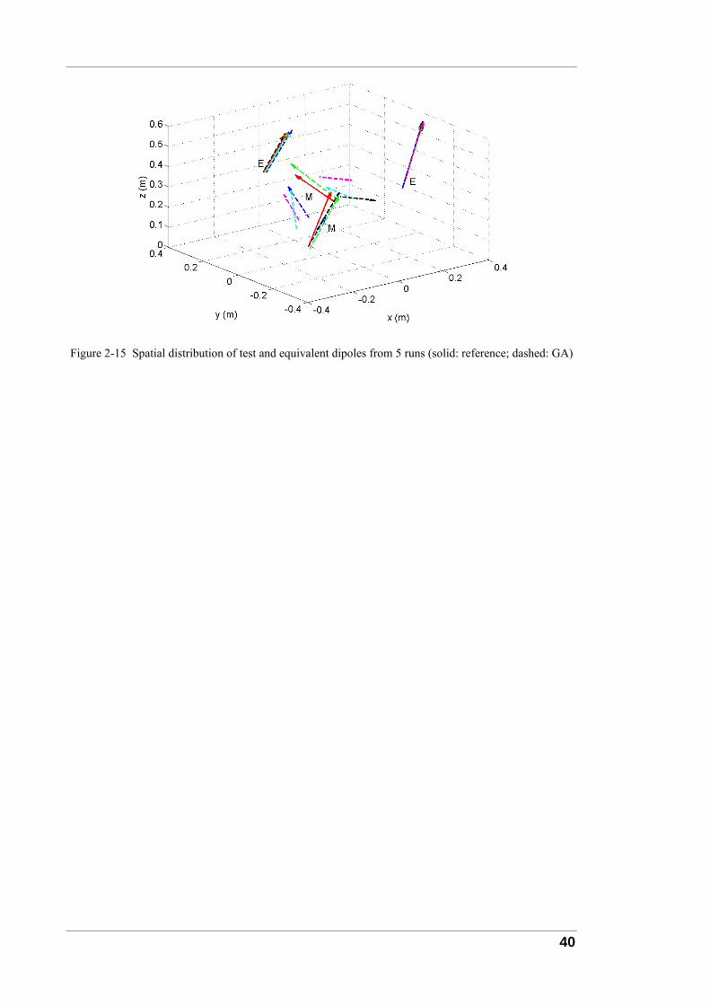
40

Figure 2-15 Spatial distribution of test and equivalent dipoles from 5 runs (solid: reference; dashed: GA)

41

3 Source Modelling of Far Field Radiation

The ultimate target of this thesis is to predict FF radiation behaviour of PCBs with

adequate accuracy. The work presented in this chapter is motivated by three issues

concerning PCB source modelling of FF radiation:

1) Using GAs to search for the equivalent infinitesimal dipole set, in order to make

the solution easily converge, an efficient way is to fix the number of dipoles N at

the beginning of the GA process. Once this is done, the GA computational

burden is proportional to N. If N is too small, the model may not be able to

reconstruct the FF radiation. If N is too large, the computational time is

unnecessarily increased and the GA may not find the optimum solution at all.

One question remains: what value of N should be chosen to minimise the

computational burden for the GA?

2) Assuming the maximum dimension of a PCB is D, when the PCB is electrically

small (D ≤ λ/10), one electric and/or one magnetic dipole is sufficient to

reconstruct the FF behaviour. In general, the FF pattern becomes more

complicated with an increasing frequency. Is it feasible to choose an appropriate

N based on the ratio of PCB size over the wavelength (D/λ)?

3) When N is too large, there are too many unknown genes to tackle. Is it possible

for GAs to get stuck in local optima? Is there any limitation in applying the GA

model?

The GA model must use sufficient dipoles to yield a good approximation for the FF, but

not necessarily for the NF. To answer the above questions, the NF-FF conversion

techniques are put aside in this chapter. FF simulated peak values for Ex, Ey and Ez

collected at sampling points are used to find an equivalent dipole set, and thus represent

the FF radiation pattern. Therefore, the effect of source modelling by GAs is verified

from the point of view of FF radiation.

By checking the difference between a FF prediction and reference data, FF tolerances

TFF,a and TFF,max were defined in (2-28) and (2-29), respectively. To evaluate the

effectiveness of a FF prediction, an appropriate number of FF observation points should

be chosen. If too few points are chosen, the maximum field magnitude point may not be

sampled, and an inaccurate TFF,max is obtained. If too many points are selected, the FF

42

prediction may be inaccurate due to the requirement of matching too many points with

small field magnitudes. In this chapter, a spherical sampling method is applied with

equally spaced elevation angles and azimuth angles, and an appropriate number of FF

points are chosen based on the classical Nyquist sampling theorem, as described in [54].

Outline

This chapter consists of 5 sections. Section 3.1 gives a clear definition of the FF region.

In Section 3.2, a small radiator, a long wire and a large loop are decomposed into a few

infinitesimal dipoles by approximating the FF radiation behaviour, respectively. In

Section 3.3, the GA is applied to model the long wire, the large loop and a power-

ground plane pair. The correlation between the number of dipoles and the ratio of PCB

size over wavelength (D/λ) is discussed, and the scope of the GA model applicability is

investigated. Section 3.4 evaluates the computational cost of GAs. Section 3.5 suggests

the number of infinitesimal dipoles required for modelling the FF of electrically small

or moderate-sized PCBs.

Contributions

The main contributions of this chapter include:

1) FF behaviour of a long wire and a large loop in free space with a certain current

distribution is analytically decomposed. With respect to FF radiation, these

typical sources can be approximated by a few infinitesimal dipoles using

theoretical methods.

2) The GA is applied to reconstruct the FF patterns of the long wire, the large loop

and a power-ground plane pair. The tolerance results and computational cost are

investigated using varying numbers of dipoles in the GA model.

3) Correlation between the number of infinitesimal dipoles in GA modelling and

the ratio of object size over wavelength (D/λ) is discussed. The GA results verify

the analytical assumptions. The scope of the model applicability is discussed and

the number of dipoles N is recommended for GA modelling.

3.1 Definition of Far Field Region

The space surrounding an electromagnetic radiation source can be divided into three

regions by the increasing distance from the source: reactive NF, radiating NF and FF

43

regions [2]. FF region is defined as that region where the angular field distribution is

essentially independent of the distance from the source; the definition of reactive and

radiating NF regions will be elaborated later in Section 4.2.

For most practical radiators, with an overall length greater than the wavelength (D > λ),

the minimum FF distance ,minFFr is defined as 2D2/λ [2]:

2

,min2 .FF

Drλ

= (3-1)

For an electrically small radiator (D ≤ λ/10), it is common to take λ as ,minFFr [2],

,min .FFr λ= (3-2)

For electrically moderate-sized sources, both (3-1) and (3-2) are extended until they join

each other at 2Dλ = . Therefore ,minFFr is chosen according to (3-1) if 2Dλ ≤ and

according to (3-2) otherwise.

3.2 Far Field Decomposition

To figure out how many infinitesimal dipoles are required to reconstruct FF radiation of

PCBs, this section first describes the FF behaviour of an electrically small radiator (D ≤

λ/10) with an arbitrary current distribution, for which one electric and/or one magnetic

dipole is enough to approximate its FF radiation.

For an electrically larger radiator, how many dipoles can represent the FF radiation with

sufficient accuracy? As it is hard to investigate the radiation of a ‘real’ PCB analytically,

some typical radiation sources with a larger size, such as a long wire and a large loop

with a certain current distribution, are then discussed. Here they are placed in free space.

The detailed field calculation for infinitesimal electric and magnetic dipoles is

elaborated in Appendix C, and the deduction for the magnetic vector potential A is

illustrated in Appendix D.

3.2.1 Small Radiator

Assume a source with a current density J(r’) and a maximum dimension D is placed at

the original point of Cartesian coordinates, as shown in Figure 3-1. According to [3][4],

the magnetic vector potential A can be written as

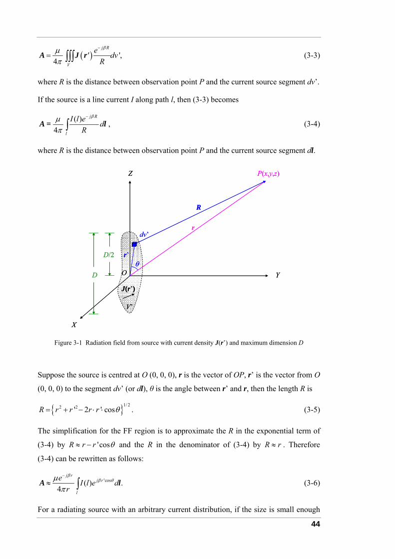
44

( ) ',4

j R

V

e' dvR

βμπ

−

= ∫∫∫A J r (3-3)

where R is the distance between observation point P and the current source segment dv’.

If the source is a line current I along path l, then (3-3) becomes

( ) ,4

j R

l

I l e dR

βμπ

−

∫A = l (3-4)

where R is the distance between observation point P and the current source segment dl.

Z

Y

P(x,y,z)

O

r

R

J(r’)

θ

X

D

D/2

dv’

r’

V’

Z

Y

P(x,y,z)

O

r

R

J(r’)

θ

X

D

D/2

dv’

r’

V’

Figure 3-1 Radiation field from source with current density J(r’) and maximum dimension D

Suppose the source is centred at O (0, 0, 0), r is the vector of OP, r’ is the vector from O

(0, 0, 0) to the segment dv’ (or dl), θ is the angle between r’ and r, then the length R is

1/ 22 2' 2 ' cos .R r r r r θ= + − ⋅ ⋅ (3-5)

The simplification for the FF region is to approximate the R in the exponential term of

(3-4) by 'cosR r r θ≈ − and the R in the denominator of (3-4) by R r≈ . Therefore

(3-4) can be rewritten as follows:

'cos( ) .4

j rj r

l

e I l e dr

ββ θμ

π

−

≈ ∫A l (3-6)

For a radiating source with an arbitrary current distribution, if the size is small enough

45

(e.g. D ≤ λ/10), the R in the exponential term of (3-4) can be approximated by R r≈ .

Therefore (3-6) can be further simplified as

( ) .4

j r

l

e I l dr

βμπ

−

≈ ∫A l (3-7)

In (3-7), the vector potential A is dependent on the summation of current instead of the

current distribution. The FF radiation can be approximated by one electric dipole when

the path l is open; and by one magnetic dipole when l is closed. If l is a combination of

an open path and a closed loop, then the FF radiation can be reconstructed by a pair of

electric and magnetic dipoles. If there is more than one open path and/or one closed

loop, it is assumed one of each dominates, and therefore one electric and/or magnetic

dipole will still be sufficient for a good FF approximation.

In summary, for an electrically small radiator, no matter how the current distributes, one

electric and/or one magnetic dipole is enough to approximate its FF radiation.

3.2.2 Long Wire

This section decomposes the FF behaviour of a long wire in free space by a few

infinitesimal dipoles. Assume a wire of length D along the z-axis (see Figure 3-2) is fed

with a current I at the centre, and the wire is very thin, i.e., when the wire diameter is

less than, say, λ/100. Considering the current along the wire is sinusoidal (see Figure

3-3), the retarded value of the current at any point z on the wire is [53]

( ) sin , 2 2mD DI z I z zβ⎡ ⎤⎛ ⎞= − ≤⎜ ⎟⎢ ⎥⎝ ⎠⎣ ⎦

(3-8)

where wave number is β = 2π/λ. This current goes to zero at the ends (for z = ± D/2).

For 2 1 , =1,2,3,2

kD kλ−= , the current I(z) at the centre (z = 0) goes to maximum

value Im ; for , =1,2,3,D k kλ= , it is zero.

In (3-8) the current is purely of standing-wave nature, and a constant phase is assumed.

The current I_cal calculated by (3-8), is shown in Figure 3-4 through Figure 3-8 for a 0.5

m long wire at 300 MHz (D = λ/2), 600 MHz (D = λ), 900 MHz (D = 3λ/2), 1.2 GHz (D

= 2λ) and 1.5 GHz (D = 5λ/2), respectively. Also included in Figure 3-4 through Figure

3-8 are the current magnitude ( )_ simulabs I and phase ( )_ simulangle I results from a

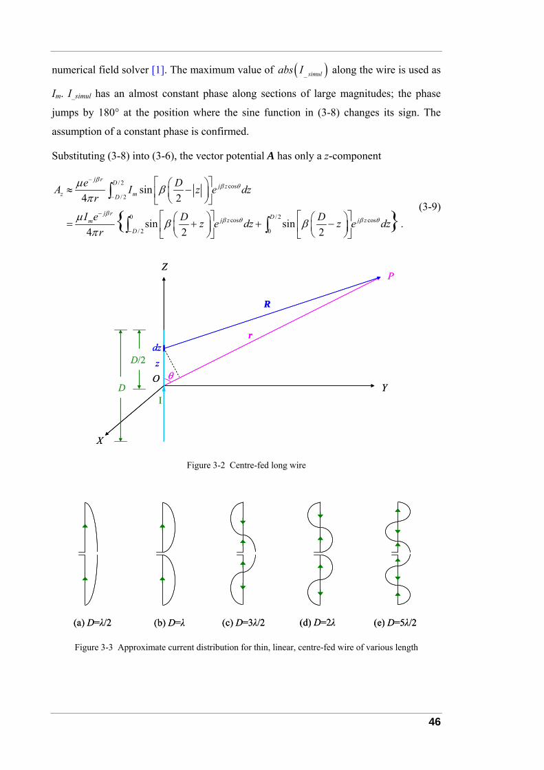
46

numerical field solver [1]. The maximum value of ( )_ simulabs I along the wire is used as

Im. I_simul has an almost constant phase along sections of large magnitudes; the phase

jumps by 180° at the position where the sine function in (3-8) changes its sign. The

assumption of a constant phase is confirmed.

Substituting (3-8) into (3-6), the vector potential A has only a z-component

/ 2 cos

/ 2

0 / 2cos cos

/ 2 0

sin4 2

sin sin .4 2 2

j r D j zz mD

j r Dj z j zmD

e DA I z e dzr

I e D Dz e dz z e dzr

ββ θ

ββ θ β θ

μ βπ

μ β βπ

−

−

−

−

⎡ ⎤⎛ ⎞≈ −⎜ ⎟⎢ ⎥⎝ ⎠⎣ ⎦⎡ ⎤ ⎡ ⎤⎛ ⎞ ⎛ ⎞= + + −⎜ ⎟ ⎜ ⎟⎢ ⎥ ⎢ ⎥⎝ ⎠ ⎝ ⎠⎣ ⎦ ⎣ ⎦

∫

∫ ∫ (3-9)

X

Z

Y

P

r

θO

R

D

D/2 zdz

I

X

Z

Y

P

r

θO

R

D

D/2 zdz

I

Figure 3-2 Centre-fed long wire

(a) D=λ/2 (b) D=λ (c) D=3λ/2 (d) D=2λ (e) D=5λ/2(a) D=λ/2 (b) D=λ (c) D=3λ/2 (d) D=2λ (e) D=5λ/2

Figure 3-3 Approximate current distribution for thin, linear, centre-fed wire of various length

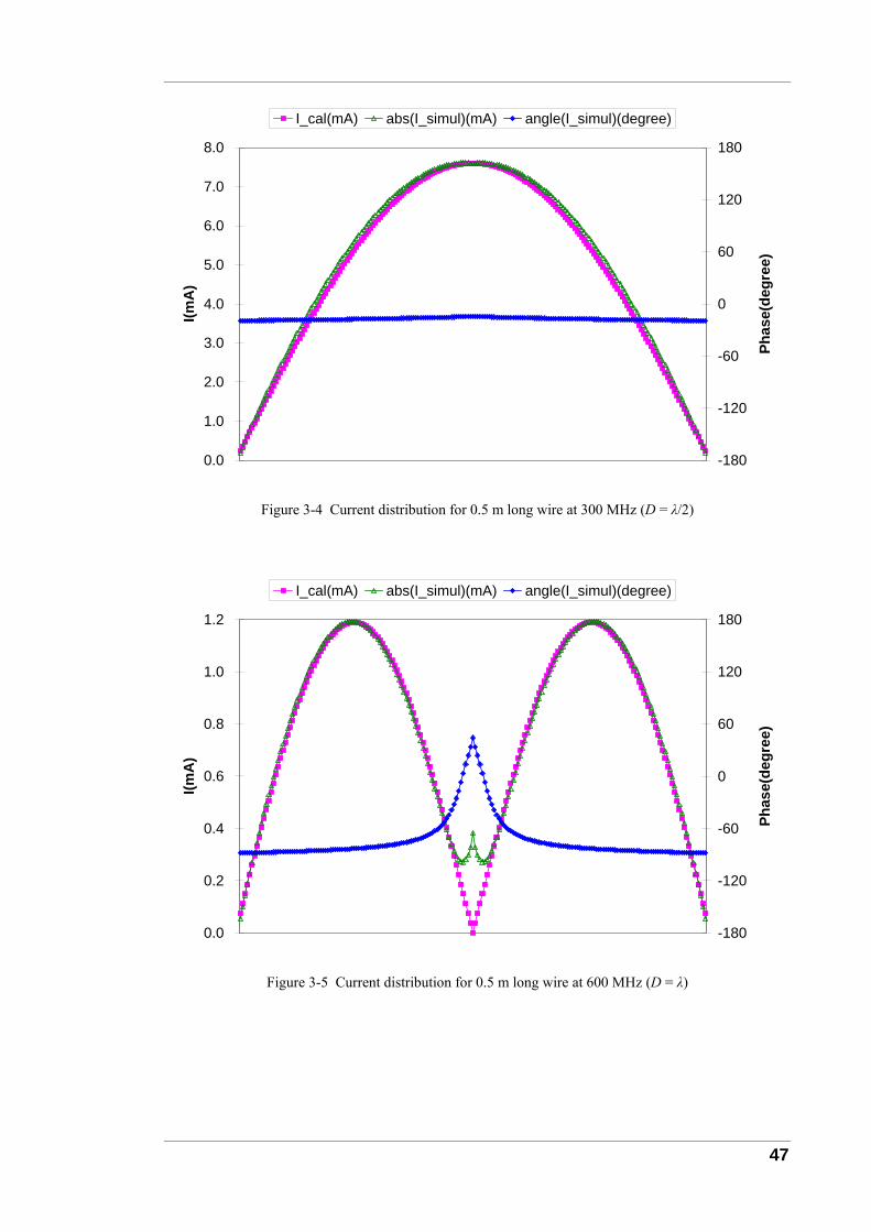
47

0.0

1.0

2.0

3.0

4.0

5.0

6.0

7.0

8.0

I(mA

)

-180

-120

-60

0

60

120

180

Phas

e(de

gree

)

I_cal(mA) abs(I_simul)(mA) angle(I_simul)(degree)

Figure 3-4 Current distribution for 0.5 m long wire at 300 MHz (D = λ/2)

0.0

0.2

0.4

0.6

0.8

1.0

1.2

I(mA

)

-180

-120

-60

0

60

120

180

Phas

e(de

gree

)

I_cal(mA) abs(I_simul)(mA) angle(I_simul)(degree)

Figure 3-5 Current distribution for 0.5 m long wire at 600 MHz (D = λ)

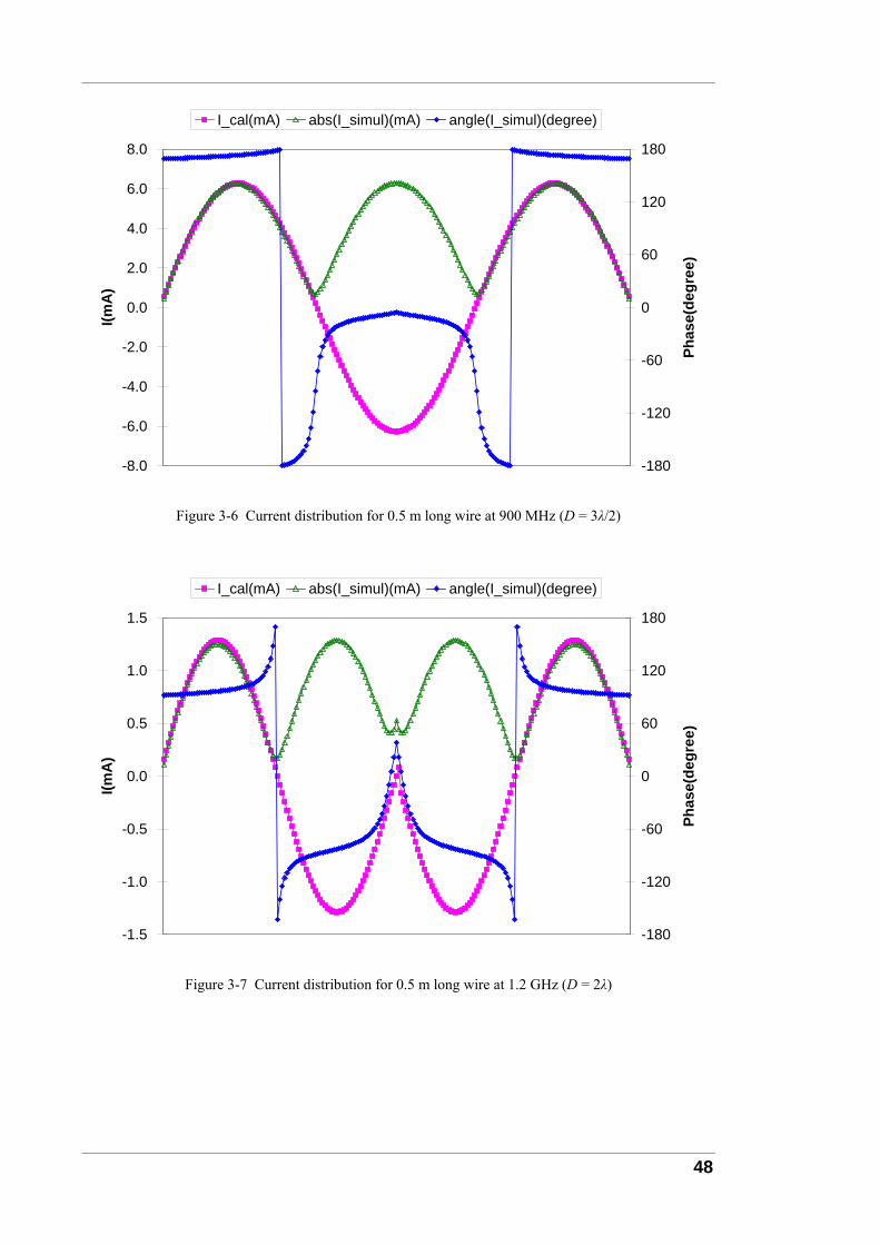
48

-8.0

-6.0

-4.0

-2.0

0.0

2.0

4.0

6.0

8.0

I(mA

)

-180

-120

-60

0

60

120

180

Phas

e(de

gree

)

I_cal(mA) abs(I_simul)(mA) angle(I_simul)(degree)

Figure 3-6 Current distribution for 0.5 m long wire at 900 MHz (D = 3λ/2)

-1.5

-1.0

-0.5

0.0

0.5

1.0

1.5

I(mA

)

-180

-120

-60

0

60

120

180

Phas

e(de

gree

)

I_cal(mA) abs(I_simul)(mA) angle(I_simul)(degree)

Figure 3-7 Current distribution for 0.5 m long wire at 1.2 GHz (D = 2λ)

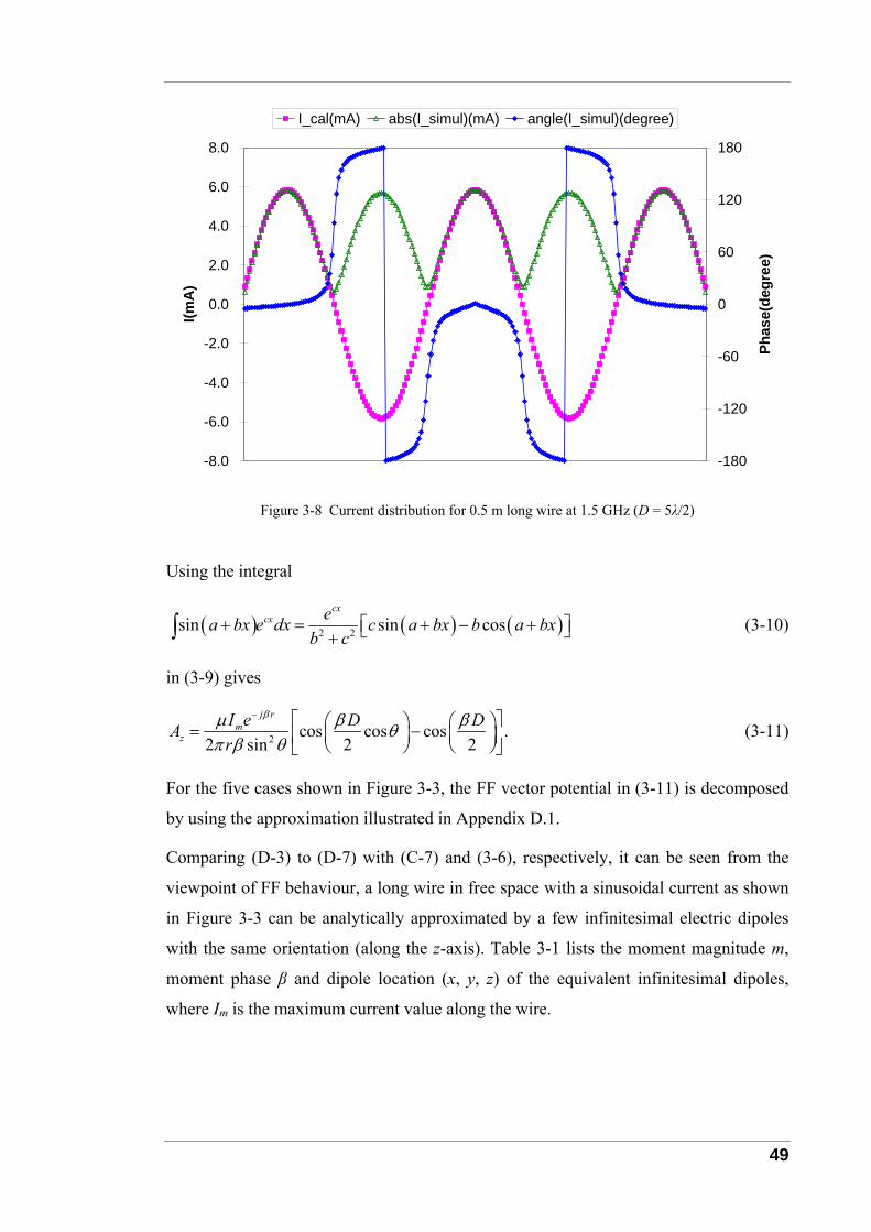
49

-8.0

-6.0

-4.0

-2.0

0.0

2.0

4.0

6.0

8.0

I(mA

)

-180

-120

-60

0

60

120

180

Phas

e(de

gree

)

I_cal(mA) abs(I_simul)(mA) angle(I_simul)(degree)

Figure 3-8 Current distribution for 0.5 m long wire at 1.5 GHz (D = 5λ/2)

Using the integral

( ) ( ) ( )2 2sin sin coscx

cx ea bx e dx c a bx b a bxb c

+ = + − +⎡ ⎤⎣ ⎦+∫ (3-10)

in (3-9) gives

2 cos cos cos .2 sin 2 2

j rm

zI e D DAr

βμ β βθπ β θ

− ⎡ ⎤⎛ ⎞ ⎛ ⎞= −⎜ ⎟ ⎜ ⎟⎢ ⎥⎝ ⎠ ⎝ ⎠⎣ ⎦ (3-11)

For the five cases shown in Figure 3-3, the FF vector potential in (3-11) is decomposed

by using the approximation illustrated in Appendix D.1.

Comparing (D-3) to (D-7) with (C-7) and (3-6), respectively, it can be seen from the

viewpoint of FF behaviour, a long wire in free space with a sinusoidal current as shown

in Figure 3-3 can be analytically approximated by a few infinitesimal electric dipoles

with the same orientation (along the z-axis). Table 3-1 lists the moment magnitude m,

moment phase β and dipole location (x, y, z) of the equivalent infinitesimal dipoles,

where Im is the maximum current value along the wire.

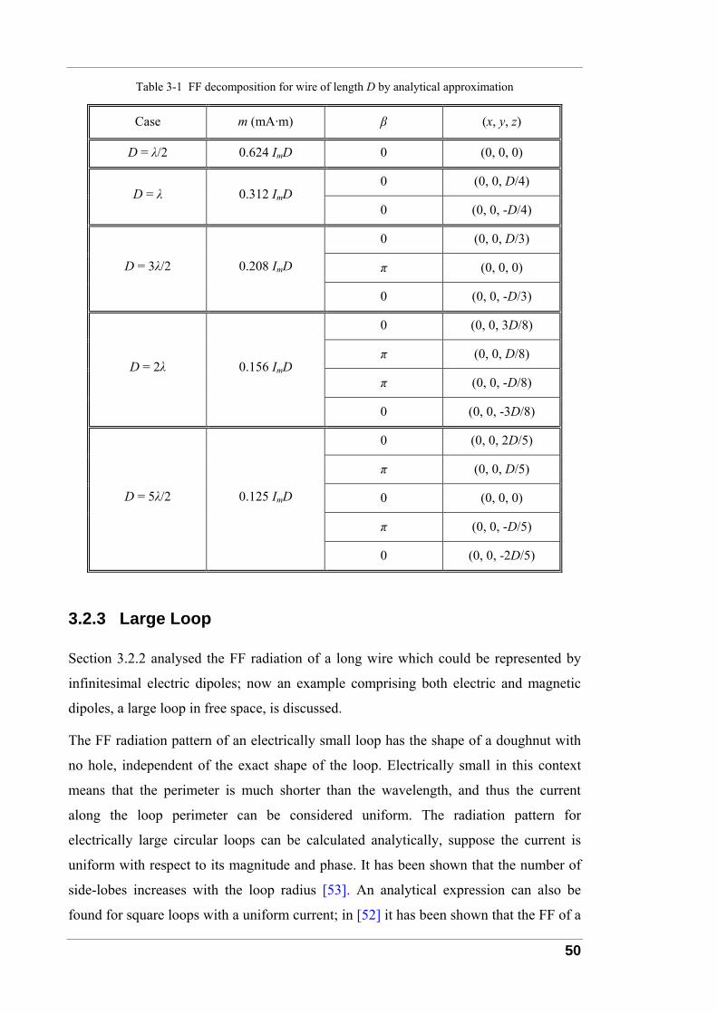
50

Table 3-1 FF decomposition for wire of length D by analytical approximation

Case m (mA·m) β (x, y, z)

D = λ/2 0.624 ImD 0 (0, 0, 0)

0 (0, 0, D/4) D = λ 0.312 ImD

0 (0, 0, -D/4)

0 (0, 0, D/3)

π (0, 0, 0) D = 3λ/2 0.208 ImD

0 (0, 0, -D/3)

0 (0, 0, 3D/8)

π (0, 0, D/8)

π (0, 0, -D/8) D = 2λ 0.156 ImD

0 (0, 0, -3D/8)

0 (0, 0, 2D/5)

π (0, 0, D/5)

0 (0, 0, 0)

π (0, 0, -D/5)

D = 5λ/2 0.125 ImD

0 (0, 0, -2D/5)

3.2.3 Large Loop

Section 3.2.2 analysed the FF radiation of a long wire which could be represented by

infinitesimal electric dipoles; now an example comprising both electric and magnetic

dipoles, a large loop in free space, is discussed.

The FF radiation pattern of an electrically small loop has the shape of a doughnut with

no hole, independent of the exact shape of the loop. Electrically small in this context

means that the perimeter is much shorter than the wavelength, and thus the current

along the loop perimeter can be considered uniform. The radiation pattern for

electrically large circular loops can be calculated analytically, suppose the current is

uniform with respect to its magnitude and phase. It has been shown that the number of

side-lobes increases with the loop radius [53]. An analytical expression can also be

found for square loops with a uniform current; in [52] it has been shown that the FF of a

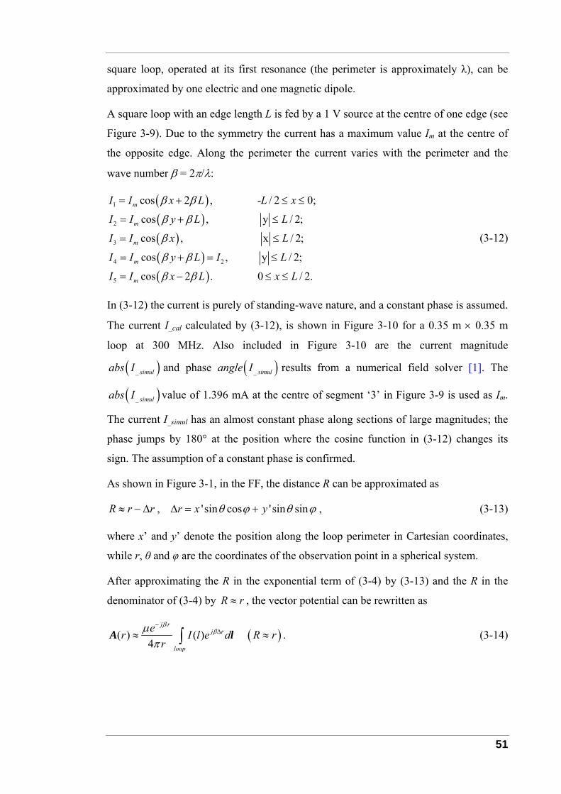
51

square loop, operated at its first resonance (the perimeter is approximately λ), can be

approximated by one electric and one magnetic dipole.

A square loop with an edge length L is fed by a 1 V source at the centre of one edge (see

Figure 3-9). Due to the symmetry the current has a maximum value Im at the centre of

the opposite edge. Along the perimeter the current varies with the perimeter and the

wave number β = 2π/λ:

( )( )( )( )( )

1

2

3

4 2

5

cos 2 , - / 2 0;

cos , y / 2;

cos , x / 2;

cos , y / 2;

cos 2 . 0 / 2.

m

m

m

m

m

I I x L L x

I I y L L

I I x L

I I y L I L

I I x L x L

β β

β β

β

β β

β β

= + ≤ ≤

= + ≤

= ≤

= + = ≤

= − ≤ ≤

(3-12)

In (3-12) the current is purely of standing-wave nature, and a constant phase is assumed.

The current I_cal calculated by (3-12), is shown in Figure 3-10 for a 0.35 m × 0.35 m

loop at 300 MHz. Also included in Figure 3-10 are the current magnitude

( )_ simulabs I and phase ( )_ simulangle I results from a numerical field solver [1]. The

( )_ simulabs I value of 1.396 mA at the centre of segment ‘3’ in Figure 3-9 is used as Im.

The current I_simul has an almost constant phase along sections of large magnitudes; the

phase jumps by 180° at the position where the cosine function in (3-12) changes its

sign. The assumption of a constant phase is confirmed.

As shown in Figure 3-1, in the FF, the distance R can be approximated as

, 'sin cos 'sin sin ,R r r r x yθ ϕ θ ϕ≈ − Δ Δ = + (3-13)

where x’ and y’ denote the position along the loop perimeter in Cartesian coordinates,

while r, θ and φ are the coordinates of the observation point in a spherical system.

After approximating the R in the exponential term of (3-4) by (3-13) and the R in the

denominator of (3-4) by R r≈ , the vector potential can be rewritten as

( )( ) ( ) .4

j rj r

loop

er I l e d R rr

ββμ

π

−Δ≈ ≈∫A l (3-14)

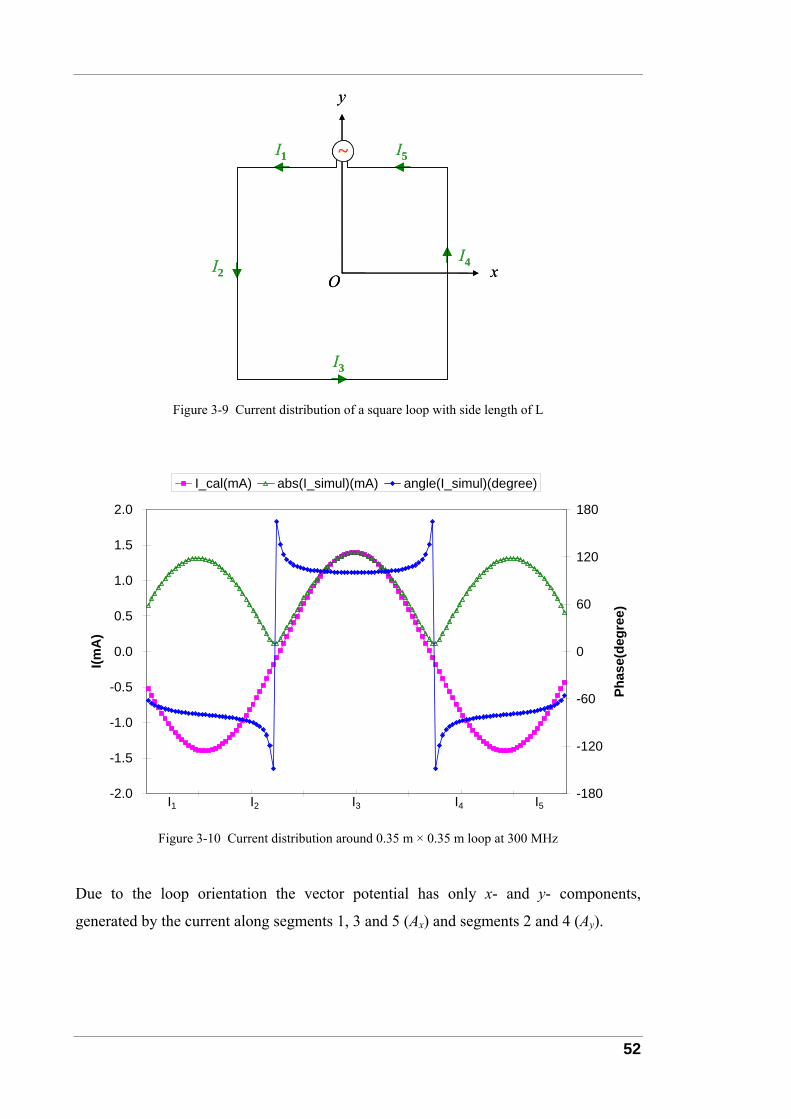
52

I1

I2

I3

I4

I5

y

xO

~I1

I2

I3

I4

I5

y

xO

~~

Figure 3-9 Current distribution of a square loop with side length of L

-2.0

-1.5

-1.0

-0.5

0.0

0.5

1.0

1.5

2.0

I(mA

)

-180

-120

-60

0

60

120

180

Phas

e(de

gree

)

I_cal(mA) abs(I_simul)(mA) angle(I_simul)(degree)

I3I2I1 I4 I5

Figure 3-10 Current distribution around 0.35 m × 0.35 m loop at 300 MHz

Due to the loop orientation the vector potential has only x- and y- components,

generated by the current along segments 1, 3 and 5 (Ax) and segments 2 and 4 (Ay).

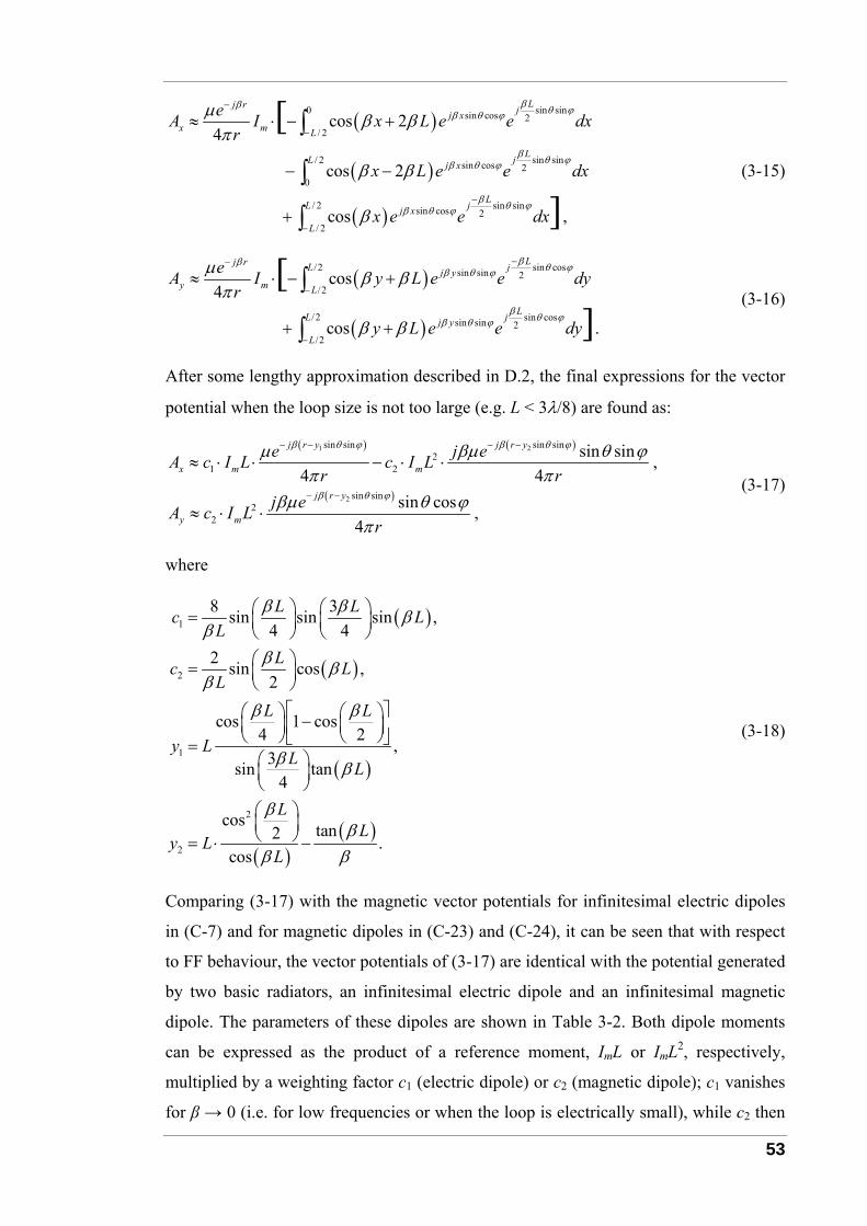
53

( )

( )

( )

0 sin sinsin cos 2/ 2

/ 2 sin sinsin cos 20

/ 2 sin sinsin cos 2/ 2

cos 24

cos 2

cos ,

[

]

Lj r jj xx m L

LL jj x

LL jj x

L

eA I x L e e dxr

x L e e dx

x e e dx

ββ θ ϕβ θ ϕ

β θ ϕβ θ ϕ

β θ ϕβ θ ϕ

μ β βπ

β β

β

−

−

−

−

≈ ⋅ − +

− −

+

∫

∫

∫

(3-15)

( )

( )

/2 sin cossin sin 2/2

/2 sin cossin sin 2/2

cos4

cos .

[]

Lj r L jj yy m L

LL jj y

L

eA I y L e e dyr

y L e e dy

ββ θ ϕβ θ ϕ

β θ ϕβ θ ϕ

μ β βπ

β β

−−

−

−

≈ ⋅ − +

+ +

∫

∫ (3-16)

After some lengthy approximation described in D.2, the final expressions for the vector

potential when the loop size is not too large (e.g. L < 3λ/8) are found as:

( ) ( )

( )

1 2

2

sin sin sin sin2

1 2

sin sin2

2

sin sin ,4 4

sin cos ,4

j r y j r y

x m m

j r y

y m

e j eA c I L c I Lr r

j eA c I Lr

β θ ϕ β θ ϕ

β θ ϕ

μ βμ θ ϕπ π

βμ θ ϕπ

− − − −

− −

≈ ⋅ ⋅ − ⋅ ⋅

≈ ⋅ ⋅

(3-17)

where

( )

( )

( )

( )( )

1

2

1

2

2

8 3sin sin sin ,4 4

2 sin cos , 2

cos 1 cos4 2 ,

3sin tan4

cos tan2 .cos

L Lc LL

Lc LL

L L

y LL L

LL

y LL

β β ββ

β ββ

β β

β β

ββ

β β

⎛ ⎞ ⎛ ⎞= ⎜ ⎟ ⎜ ⎟⎝ ⎠ ⎝ ⎠⎛ ⎞= ⎜ ⎟⎝ ⎠

⎡ ⎤⎛ ⎞ ⎛ ⎞−⎜ ⎟ ⎜ ⎟⎢ ⎥⎝ ⎠ ⎝ ⎠⎣ ⎦=⎛ ⎞⎜ ⎟⎝ ⎠⎛ ⎞⎜ ⎟⎝ ⎠= ⋅ −

(3-18)

Comparing (3-17) with the magnetic vector potentials for infinitesimal electric dipoles

in (C-7) and for magnetic dipoles in (C-23) and (C-24), it can be seen that with respect

to FF behaviour, the vector potentials of (3-17) are identical with the potential generated

by two basic radiators, an infinitesimal electric dipole and an infinitesimal magnetic

dipole. The parameters of these dipoles are shown in Table 3-2. Both dipole moments

can be expressed as the product of a reference moment, ImL or ImL2, respectively,

multiplied by a weighting factor c1 (electric dipole) or c2 (magnetic dipole); c1 vanishes

for β → 0 (i.e. for low frequencies or when the loop is electrically small), while c2 then

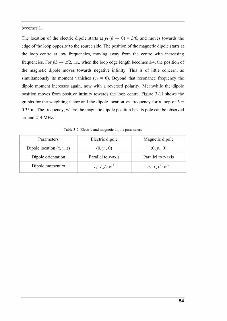
54

becomes 1.

The location of the electric dipole starts at y1 (β → 0) = L/6, and moves towards the

edge of the loop opposite to the source side. The position of the magnetic dipole starts at

the loop centre at low frequencies, moving away from the centre with increasing

frequencies. For βL → π/2, i.e., when the loop edge length becomes λ/4, the position of

the magnetic dipole moves towards negative infinity. This is of little concern, as

simultaneously its moment vanishes (c2 = 0). Beyond that resonance frequency the

dipole moment increases again, now with a reversed polarity. Meanwhile the dipole

position moves from positive infinity towards the loop centre. Figure 3-11 shows the

graphs for the weighting factor and the dipole location vs. frequency for a loop of L =

0.35 m. The frequency, where the magnetic dipole position has its pole can be observed

around 214 MHz.

Table 3-2 Electric and magnetic dipole parameters

Parameters Electric dipole Magnetic dipole

Dipole location (x, y, z) (0, y1, 0) (0, y2, 0)

Dipole orientation Parallel to x-axis Parallel to z-axis

Dipole moment m 01

jmc I L e⋅ ⋅ 2

2j

mc I L e π⋅ ⋅

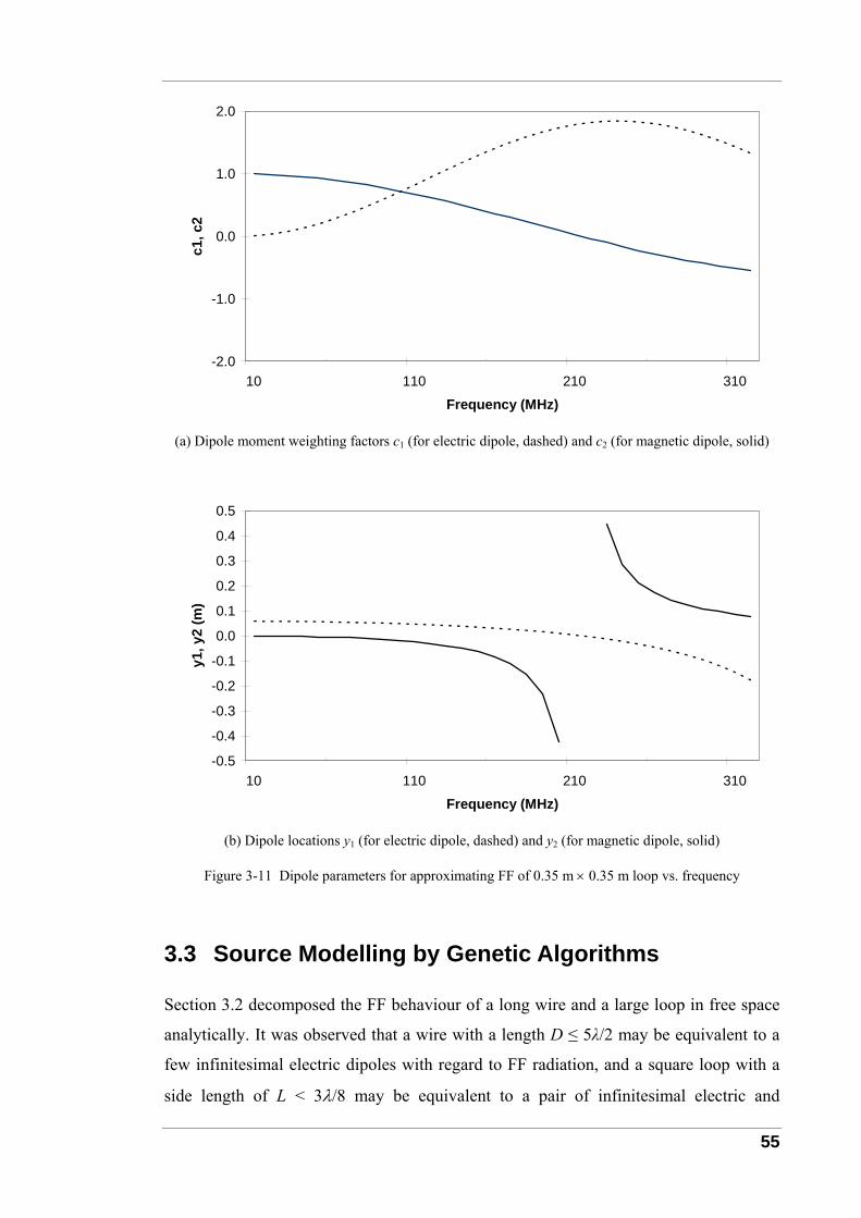
55

-2.0

-1.0

0.0

1.0

2.0

10 110 210 310

Frequency (MHz)

c1, c

2

(a) Dipole moment weighting factors c1 (for electric dipole, dashed) and c2 (for magnetic dipole, solid)

-0.5

-0.4

-0.3

-0.2

-0.1

0.0

0.1

0.2

0.3

0.4

0.5

10 110 210 310

Frequency (MHz)

y1, y

2 (m

)

(b) Dipole locations y1 (for electric dipole, dashed) and y2 (for magnetic dipole, solid)

Figure 3-11 Dipole parameters for approximating FF of 0.35 m × 0.35 m loop vs. frequency

3.3 Source Modelling by Genetic Algorithms

Section 3.2 decomposed the FF behaviour of a long wire and a large loop in free space

analytically. It was observed that a wire with a length D ≤ 5λ/2 may be equivalent to a

few infinitesimal electric dipoles with regard to FF radiation, and a square loop with a

side length of L < 3λ/8 may be equivalent to a pair of infinitesimal electric and

56

magnetic dipoles. This section applies the GA of Chapter 2 to find the parameters of

these infinitesimal dipoles.

In a good PCB design, long wires and large loops are usually avoided. To make clear

how many dipoles are required to reconstruct the FF of a PCB, as a commonly used

structure with possibly significant radiation, a power-ground plane pair is also to be

investigated. In [55]-[57], the FF radiation of power-ground planes was calculated using

a cavity model. It was shown, that for realistic dimensions, the radiation from such a

structure was equivalent to a magnetic line current along the edge.

For the long wire to be checked in Section 3.3.1, the dipole type is limited to be electric;

while for the large loop and the power-ground plane pair to be verified in Section 3.3.2

and 3.3.3, the dipole type can be both electric and magnetic. Unless otherwise specified,

the GA parameters for selection mentioned in Figure 2-6 are: population size K = 102,

subgroup population size M = 20 and elite database size 10N = 50. To get a global

optimum, in this chapter the best NF match among 5 GA runs is picked up as the

optimum solution.

3.3.1 Long Wire

This section applies GAs to reconstruct the FF pattern of a 0.5 m long wire in free space

[48]. A 0.5 m long wire with a diameter of 0.2 mm is excited by 1 V, 50 Ω at its centre.

One end of the wire is located at point (-L/2, -W/2, h1), and the other at (L/2, W/2, h2),

where L = W = 350 mm, h1 = 2 mm, h2 = 12 mm.

Figure 3-12 shows the input impedance Zin of the long wire at varying frequencies (30

MHz - 3 GHz), as well as the five frequency points to be investigated in detail, 300

MHz, 600 MHz, 900 MHz, 1.2 GHz and 1.5 GHz. At 300 MHz, 900 MHz and 1.5GHz,

Zin is a minimum, indicating a maximum current injected into the wire, and

consequently the FF radiation has significant magnitudes. At 600 MHz and 1.2 GHz, Zin

is close to a local maximum, and thus the FF radiation has weak magnitudes.

As referred to at the beginning of this chapter, instead of applying NF-FF conversion

techniques, the GA model now focuses on pure FF reconstruction. FF data are input into

the GA model to search for the equivalent dipole set, and then represent the FF radiation

pattern. Electric FF data on a sphere of r = 5 m are obtained by a simulation [1]. Similar

to (2-19) and (2-27), the fitness function for the GA model is defined as follows:

57

0

1000

2000

3000

4000

5000

6000

0 500 1000 1500 2000 2500 3000

Frequency (MHz)

Zin

(Ohm

)

Zin (Ohm)Frequencies investigated

Figure 3-12 Input impedance of long wire at various frequencies

( ),

1

1 ,20 lg lg

k M

m m km

F sv f

M =

=⋅ −∑

(3-19)

where vm and fm,k mean the FF magnitudes Ex, Ey and Ez among (peak values among all

phase intervals) at M sampling points. FF tolerances TFF,a and TFF,max are calculated

according to (2-28) and (2-29) respectively. The generation number G = 200 is used

unless otherwise specified.

For each dipole the type is fixed as electric (K = 1), and optimum parameters for the

other 7 genes (see Section 2.2) are searched by the GA model. Figure 3-13 and Figure

3-14 plot the FF tolerance results, for varying numbers of infinitesimal electric dipoles

N in the GA model at all five frequencies. Table 3-4 compares the FF tolerances of the

GA model with those of the analytical solution. Figure 3-15 to Figure 3-19 compare the

FF patterns generated by the GA dipoles with the reference data. Figure 3-20 to Figure

3-24 show the spatial distribution of the GA dipoles.

3.3.1.1 300 MHz – 1.2 GHz

At 300 MHz, 1 infinitesimal dipole is enough to describe the electric FF pattern, since

the pattern is quite simple as shown in Figure 3-15. Table 3-3 compares the dipole set

(n1) obtained by the GA with the original set (t1) obtained by analytical approximation

58

in Table 3-1. In Table 3-3, angles and phases are expressed in rad, and spatial

coordinates in mm. Since no phase information is used as input NF data of GA, the

phase value of the GA dipole set (n1) is normalised by subtracting 2.89 rad.

From Table 3-3, at 300 MHz, the GA result of dipole moment magnitude (2.42 mA⋅m)

is very close to the analytical calculation (2.40 mA⋅m). The dipole orientation is exactly

found by the GA model, and the deviation of the GA dipole location from the analytical

solution is also small (less than 13 mm in respect of an overall wire length of 0.5 m).

The spatial distribution of the GA dipoles shown in Figure 3-20 matches with the

analytical approximation illustrated in Table 3-1.

As mentioned in Section 1.1, for an acceptable FF prediction, 1.5 dB is suggested to be

the maximum allowable tolerance. From Table 3-4, at 300 MHz, both methods reach

comparably good FF prediction (TFF,max = 0.32 – 0.38 dB, TFF,a = 0.45 – 0.46 dB).

Therefore for a wire with D = λ/2, 1 infinitesimal electric dipole located at the centre of

the original wire can well reconstruct its FF pattern, whose parameters are effectively

searched by the GA.

From Figure 3-13, Figure 3-14 and Table 3-4, it can be seen that at 600 MHz (D = λ), 2

dipoles searched by the GA can approximate the FF pattern of this 0.5 m long wire with

accuracy (TFF,max = 0.06 dB, TFF,a = 0.35 dB), however it is not possible for 1 dipole to

obtain an acceptable prediction. The spatial distribution of these two equivalent electric

dipoles is shown in Figure 3-21. The moment phase, dipole location and orientation

found by the GA are close to the analytical result listed in Table 3-1.

Unlike the perfect match between I_cal and I_simul at 300 MHz shown in Figure 3-5,

minor difference exists at 600 MHz. For example, at the wire centre, I_cal is assumed to

be 0; however I_simul does not go to 0, and a phase oscillation around that point is

observed. Furthermore, as indicated in Appendix D.1.2, the analytical solution uses the

approximations of (D-1) and from (D-2) to (D-3). However, GAs are a different

approach which in this case only focuses on the FF radiation itself. That is why the GA

model can reach better FF approximation than the analytical solution (see Table 3-4).

Figure 3-13, Figure 3-14 and Table 3-4 show that at 900MHz (D = 3λ/2), 3 GA dipoles

can well reconfigure the pattern (TFF,max = 0.24 dB, TFF,a = 0.47 dB). From Figure 3-22,

the moment phase and dipole orientation of these three dipoles match with the analytical

assumption in Table 3-1.

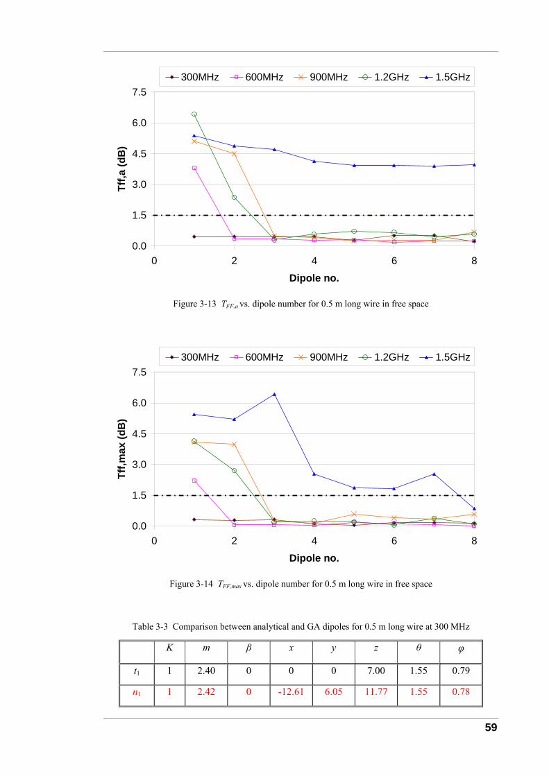
59

0.0

1.5

3.0

4.5

6.0

7.5

0 2 4 6 8

Dipole no.

Tff,a

(dB

)

300MHz 600MHz 900MHz 1.2GHz 1.5GHz

Figure 3-13 TFF,a vs. dipole number for 0.5 m long wire in free space

0.0

1.5

3.0

4.5

6.0

7.5

0 2 4 6 8

Dipole no.

Tff,m

ax (d

B)

300MHz 600MHz 900MHz 1.2GHz 1.5GHz

Figure 3-14 TFF,max vs. dipole number for 0.5 m long wire in free space

Table 3-3 Comparison between analytical and GA dipoles for 0.5 m long wire at 300 MHz

K m β x y z θ φ

t1 1 2.40 0 0 0 7.00 1.55 0.79

n1 1 2.42 0 -12.61 6.05 11.77 1.55 0.78

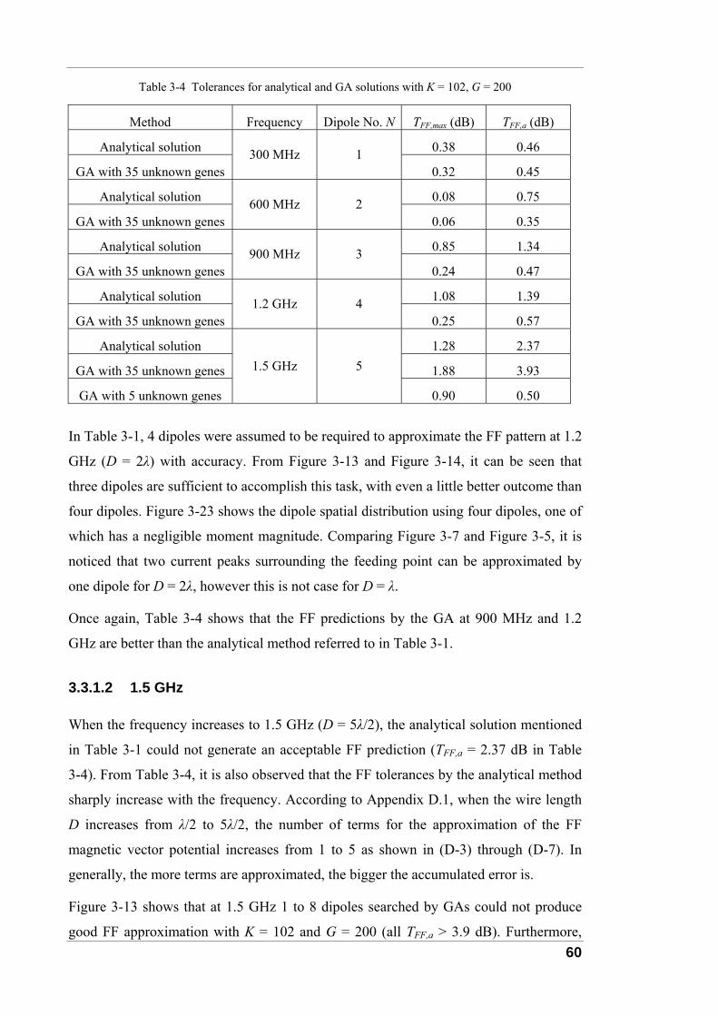
60

Table 3-4 Tolerances for analytical and GA solutions with K = 102, G = 200

Method Frequency Dipole No. N TFF,max (dB) TFF,a (dB)

Analytical solution 0.38 0.46

GA with 35 unknown genes 300 MHz 1

0.32 0.45

Analytical solution 0.08 0.75

GA with 35 unknown genes 600 MHz 2

0.06 0.35

Analytical solution 0.85 1.34

GA with 35 unknown genes 900 MHz 3

0.24 0.47

Analytical solution 1.08 1.39

GA with 35 unknown genes 1.2 GHz 4

0.25 0.57

Analytical solution 1.28 2.37

GA with 35 unknown genes 1.88 3.93

GA with 5 unknown genes

1.5 GHz 5

0.90 0.50

In Table 3-1, 4 dipoles were assumed to be required to approximate the FF pattern at 1.2

GHz (D = 2λ) with accuracy. From Figure 3-13 and Figure 3-14, it can be seen that

three dipoles are sufficient to accomplish this task, with even a little better outcome than

four dipoles. Figure 3-23 shows the dipole spatial distribution using four dipoles, one of

which has a negligible moment magnitude. Comparing Figure 3-7 and Figure 3-5, it is

noticed that two current peaks surrounding the feeding point can be approximated by

one dipole for D = 2λ, however this is not case for D = λ.

Once again, Table 3-4 shows that the FF predictions by the GA at 900 MHz and 1.2

GHz are better than the analytical method referred to in Table 3-1.

3.3.1.2 1.5 GHz

When the frequency increases to 1.5 GHz (D = 5λ/2), the analytical solution mentioned

in Table 3-1 could not generate an acceptable FF prediction (TFF,a = 2.37 dB in Table

3-4). From Table 3-4, it is also observed that the FF tolerances by the analytical method

sharply increase with the frequency. According to Appendix D.1, when the wire length

D increases from λ/2 to 5λ/2, the number of terms for the approximation of the FF

magnetic vector potential increases from 1 to 5 as shown in (D-3) through (D-7). In

generally, the more terms are approximated, the bigger the accumulated error is.

Figure 3-13 shows that at 1.5 GHz 1 to 8 dipoles searched by GAs could not produce

good FF approximation with K = 102 and G = 200 (all TFF,a > 3.9 dB). Furthermore,

61

with other GA parameters kept the same as before, increasing K from 102 to 202, or

extending G from 200 to 400 or 800 does not improve the FF approximation.

Figure 3-19 (a) shows the 3-D and 2-D reference FF patterns at 1.5 GHz. There are 5

lobes, 3 of which are closely packed. This pattern is the most complicated one among

all five frequencies investigated.

For N = 5, the above GA model needs to tackle 35 unknown genes since the dipole type

is fixed as electric. In order to check whether less unknown genes improve the GA

searching ability or not, genes other than moment magnitudes mq are fixed per the

analytical approximation in Table 3-1. Therefore the GA model only copes with 5

unknown genes (mq), and other GA parameters are kept the same as before: K = 102, G

= 200. Figure 3-19 compares the FF patterns generated in two GA cases (35 unknown

genes and 5 unknown genes) with the reference data. By reducing the unknown genes

from 35 to 5, the GA no longer tends to get stuck at local optima but dramatically

improves the searching results (TFF,max = 0.90 dB vs. 1.88 dB, TFF,a = 0.50 dB vs. 3.93

dB in Table 3-4).

Table 3-5 compares the dipole set (t1, t2, t3, t4, t5) obtained by analytical decomposition

mentioned in Table 3-1 with the GA results. The dipole set (n1, n2, n3, n4, n5) represents

the equivalent dipole set searched by the GA with 35 unknown genes, while (n1’, n2’,

n3’, n4’, n5’) means the dipole set obtained by the GA with 5 unknown genes. It is

observed from Table 3-4 and Table 3-5 that from the analytical solution to the GA result

with 5 unknown genes, a slight adjustment about the dipole moment magnitude among

5 dipoles brings about a huge improvement on the FF tolerances. TFF,max drops from

1.28 dB to 0.90 dB, and TFF,a is decreased from 2.37 dB to 0.50. This confirms that the

global optimum solution is surrounded by many local optima for this example.

Figure 3-24 compares the spatial distribution of the electric dipole sets in both GA cases.

In this example, with 35 unknown genes, it is very hard for the GA model to reach the

symmetrical distribution of dipole location and orientation, and therefore TFF,a is as high

as 3.93 dB. From Figure 3-19 (c), it can be seen with 5 unknown genes, the three

closely packed lobes in the FF pattern are reconstructed by the GA model.

As indicated at the beginning of Section 2.5.3, due to the tendency of getting stuck in

local optima, GAs sometimes may not be able to find the global optimum. This D =

5λ/2 case shows the limitation of the GA model applicability, when the global optimum

solution is surrounded by lots of local optima. When the operating frequency goes

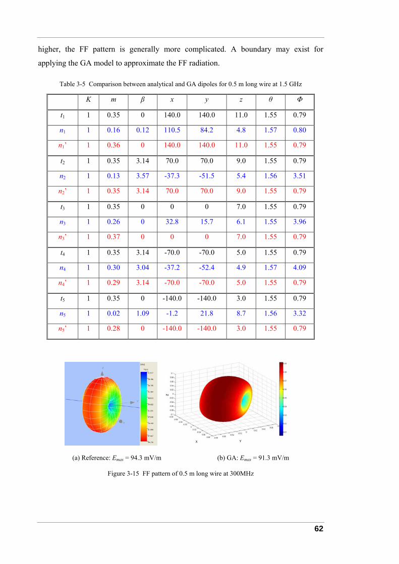
62

higher, the FF pattern is generally more complicated. A boundary may exist for

applying the GA model to approximate the FF radiation.

Table 3-5 Comparison between analytical and GA dipoles for 0.5 m long wire at 1.5 GHz

K m β x y z θ Φ

t1 1 0.35 0 140.0 140.0 11.0 1.55 0.79

n1 1 0.16 0.12 110.5 84.2 4.8 1.57 0.80

n1’ 1 0.36 0 140.0 140.0 11.0 1.55 0.79

t2 1 0.35 3.14 70.0 70.0 9.0 1.55 0.79

n2 1 0.13 3.57 -37.3 -51.5 5.4 1.56 3.51

n2’ 1 0.35 3.14 70.0 70.0 9.0 1.55 0.79

t3 1 0.35 0 0 0 7.0 1.55 0.79

n3 1 0.26 0 32.8 15.7 6.1 1.55 3.96

n3’ 1 0.37 0 0 0 7.0 1.55 0.79

t4 1 0.35 3.14 -70.0 -70.0 5.0 1.55 0.79

n4 1 0.30 3.04 -37.2 -52.4 4.9 1.57 4.09

n4’ 1 0.29 3.14 -70.0 -70.0 5.0 1.55 0.79

t5 1 0.35 0 -140.0 -140.0 3.0 1.55 0.79

n5 1 0.02 1.09 -1.2 21.8 8.7 1.56 3.32

n5’ 1 0.28 0 -140.0 -140.0 3.0 1.55 0.79

(a) Reference: Emax = 94.3 mV/m (b) GA: Emax = 91.3 mV/m

Figure 3-15 FF pattern of 0.5 m long wire at 300MHz

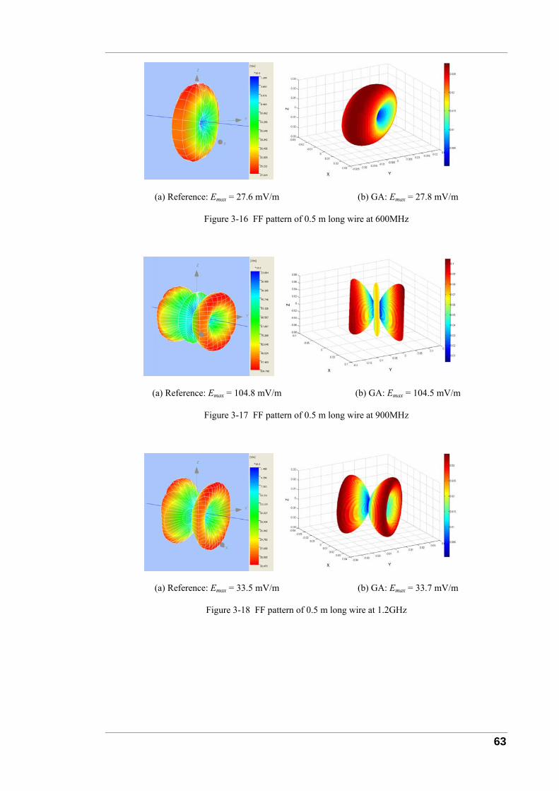
63

(a) Reference: Emax = 27.6 mV/m (b) GA: Emax = 27.8 mV/m

Figure 3-16 FF pattern of 0.5 m long wire at 600MHz

(a) Reference: Emax = 104.8 mV/m (b) GA: Emax = 104.5 mV/m

Figure 3-17 FF pattern of 0.5 m long wire at 900MHz

(a) Reference: Emax = 33.5 mV/m (b) GA: Emax = 33.7 mV/m

Figure 3-18 FF pattern of 0.5 m long wire at 1.2GHz

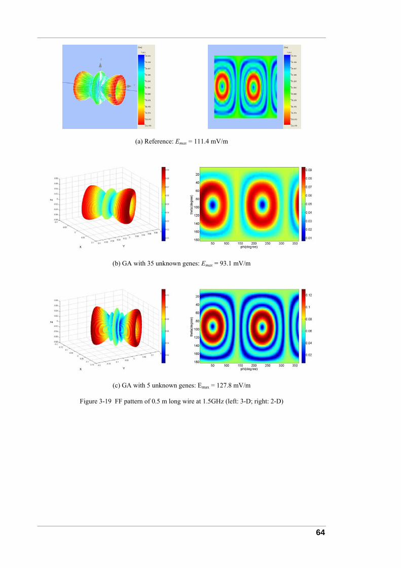
64

(a) Reference: Emax = 111.4 mV/m

(b) GA with 35 unknown genes: Emax = 93.1 mV/m

(c) GA with 5 unknown genes: Emax = 127.8 mV/m

Figure 3-19 FF pattern of 0.5 m long wire at 1.5GHz (left: 3-D; right: 2-D)

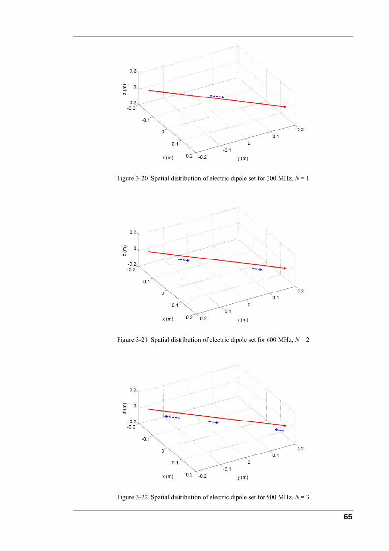
65

Figure 3-20 Spatial distribution of electric dipole set for 300 MHz, N = 1

Figure 3-21 Spatial distribution of electric dipole set for 600 MHz, N = 2

Figure 3-22 Spatial distribution of electric dipole set for 900 MHz, N = 3

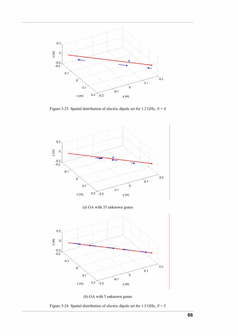
66

Figure 3-23 Spatial distribution of electric dipole set for 1.2 GHz, N = 4

(a) GA with 35 unknown genes

(b) GA with 5 unknown genes

Figure 3-24 Spatial distribution of electric dipole set for 1.5 GHz, N = 5

67

3.3.2 Large Loop

Section 3.2.3 calculated the FF of a square loop with an edge length of L < 3λ/8. Rather

than using the analytical expression in (3-18), GAs are now used to determine the

location, orientation and moment of the two dipoles for reconstructing the FF radiation.

For the 0.35 m × 0.35 m loop at 300 MHz (D = λ/2) mentioned in Section 3.2.3, electric

FF data at a sphere of r = 5 m are obtained by the Concept-II software [1]. Based on the

same fitness and FF tolerance calculation methods mentioned in Section 3.3.1, the

optimum infinitesimal electric and magnetic dipoles for reconstructing the FF radiation

are obtained by the GA model. G = 400 is used here.

The GA solutions are compared to the analytical results in Table 3-6. The dipole

location and moment are also shown in Figure 3-25.

There is a good agreement between the analytical and GA dipoles with respect to the

dipole location, moment and phase. The GA solution is based on magnitude-only data,

and the dipole moment phase is therefore arbitrary; the important criterion is the phase

difference between electric and magnetic dipole moments. The phase difference in the

analytical solution is exactly π rad, very close to the GA solution, 3.10 rad.

To compare the quality of both results, polar diagrams for the FF radiation are shown in

Figure 3-26. The graphs depict the vertical diagram, with θ varying from 0 to 360°,

while φ is kept at 30°, and the horizontal diagram with a varying φ and a constant θ =

90°. The solid curves are the reference data from the numerical simulation, the dotted

curves are for the dipoles obtained analytically, and the dashed curves show results

from the GA dipoles.

Source modelling by only two infinitesimal dipoles already shows very good results.

Both methods reach a very good predicition for the maximum field strength (TFF,max <

0.5 dB). With respect to the radiation pattern, the GA dipoles actually match the

reference data better than the dipoles from the analytical approximation, both according

to the polar diagrams of Figure 3-26 and the tolerance values of Table 3-7 (TFF,a = 0.42

vs. 0.95 dB). After all, the analytical solution is based on: (i) an approximation for the

current distribution along the loop perimeter in (3-12); and (ii) approximations for the

vector potential when going from (3-15) and (3-16) to (3-17) and (3-18).

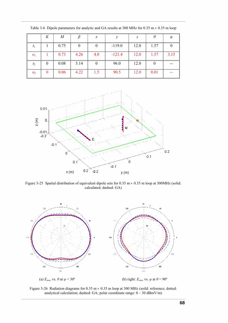
68

Table 3-6 Dipole parameters for analytic and GA results at 300 MHz for 0.35 m × 0.35 m loop

K M β x y z θ φ

t1 1 0.75 0 0 -119.0 12.0 1.57 0

n1 1 0.73 4.26 4.0 -121.4 12.0 1.57 3.15

t2 0 0.08 3.14 0 96.0 12.0 0 --

n2 0 0.06 4.22 1.5 90.5 12.0 0.01 --

Figure 3-25 Spatial distribution of equivalent dipole sets for 0.35 m × 0.35 m loop at 300MHz (solid: calculated; dashed: GA)

(a) Emax vs. θ at φ = 30º (b) right: Emax vs. φ at θ = 90º

Figure 3-26 Radiation diagrams for 0.35 m × 0.35 m loop at 300 MHz (soild: reference; dotted: analytical calculation; dashed: GA; polar coordinate range: 0 – 30 dBmV/m)

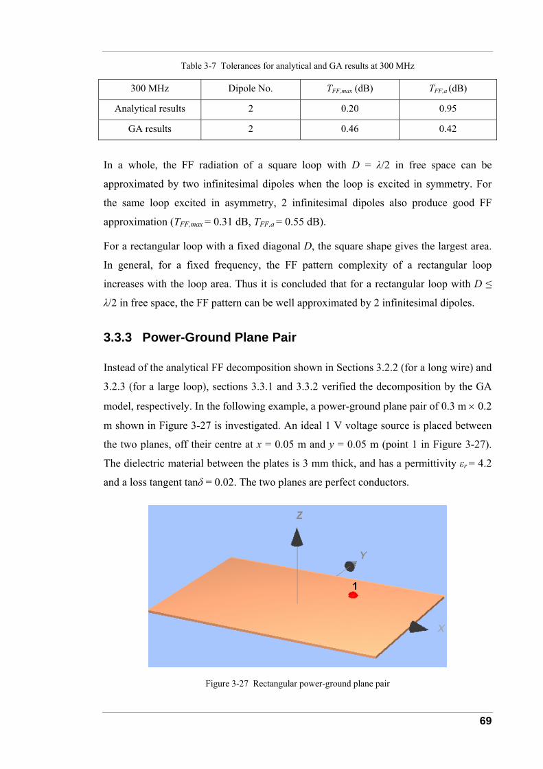
69

Table 3-7 Tolerances for analytical and GA results at 300 MHz

300 MHz Dipole No. TFF,max (dB) TFF,a (dB)

Analytical results 2 0.20 0.95

GA results 2 0.46 0.42

In a whole, the FF radiation of a square loop with D = λ/2 in free space can be

approximated by two infinitesimal dipoles when the loop is excited in symmetry. For

the same loop excited in asymmetry, 2 infinitesimal dipoles also produce good FF

approximation (TFF,max = 0.31 dB, TFF,a = 0.55 dB).

For a rectangular loop with a fixed diagonal D, the square shape gives the largest area.

In general, for a fixed frequency, the FF pattern complexity of a rectangular loop

increases with the loop area. Thus it is concluded that for a rectangular loop with D ≤

λ/2 in free space, the FF pattern can be well approximated by 2 infinitesimal dipoles.

3.3.3 Power-Ground Plane Pair

Instead of the analytical FF decomposition shown in Sections 3.2.2 (for a long wire) and

3.2.3 (for a large loop), sections 3.3.1 and 3.3.2 verified the decomposition by the GA

model, respectively. In the following example, a power-ground plane pair of 0.3 m × 0.2

m shown in Figure 3-27 is investigated. An ideal 1 V voltage source is placed between

the two planes, off their centre at x = 0.05 m and y = 0.05 m (point 1 in Figure 3-27).

The dielectric material between the plates is 3 mm thick, and has a permittivity εr = 4.2

and a loss tangent tanδ = 0.02. The two planes are perfect conductors.

Figure 3-27 Rectangular power-ground plane pair

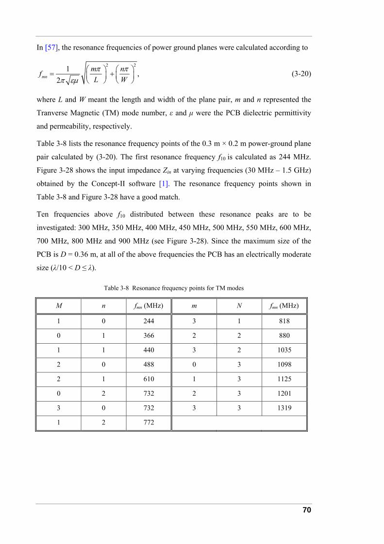
70

In [57], the resonance frequencies of power ground planes were calculated according to

2 21 ,2mn

m nfL Wπ π

π εμ⎛ ⎞ ⎛ ⎞= +⎜ ⎟ ⎜ ⎟⎝ ⎠ ⎝ ⎠

(3-20)

where L and W meant the length and width of the plane pair, m and n represented the

Tranverse Magnetic (TM) mode number, ε and μ were the PCB dielectric permittivity

and permeability, respectively.

Table 3-8 lists the resonance frequency points of the 0.3 m × 0.2 m power-ground plane

pair calculated by (3-20). The first resonance frequency f10 is calculated as 244 MHz.

Figure 3-28 shows the input impedance Zin at varying frequencies (30 MHz – 1.5 GHz)

obtained by the Concept-II software [1]. The resonance frequency points shown in

Table 3-8 and Figure 3-28 have a good match.

Ten frequencies above f10 distributed between these resonance peaks are to be

investigated: 300 MHz, 350 MHz, 400 MHz, 450 MHz, 500 MHz, 550 MHz, 600 MHz,

700 MHz, 800 MHz and 900 MHz (see Figure 3-28). Since the maximum size of the

PCB is D = 0.36 m, at all of the above frequencies the PCB has an electrically moderate

size (λ/10 < D ≤ λ).

Table 3-8 Resonance frequency points for TM modes

M n fmn (MHz) m N fmn (MHz)

1 0 244 3 1 818

0 1 366 2 2 880

1 1 440 3 2 1035

2 0 488 0 3 1098

2 1 610 1 3 1125

0 2 732 2 3 1201

3 0 732 3 3 1319

1 2 772

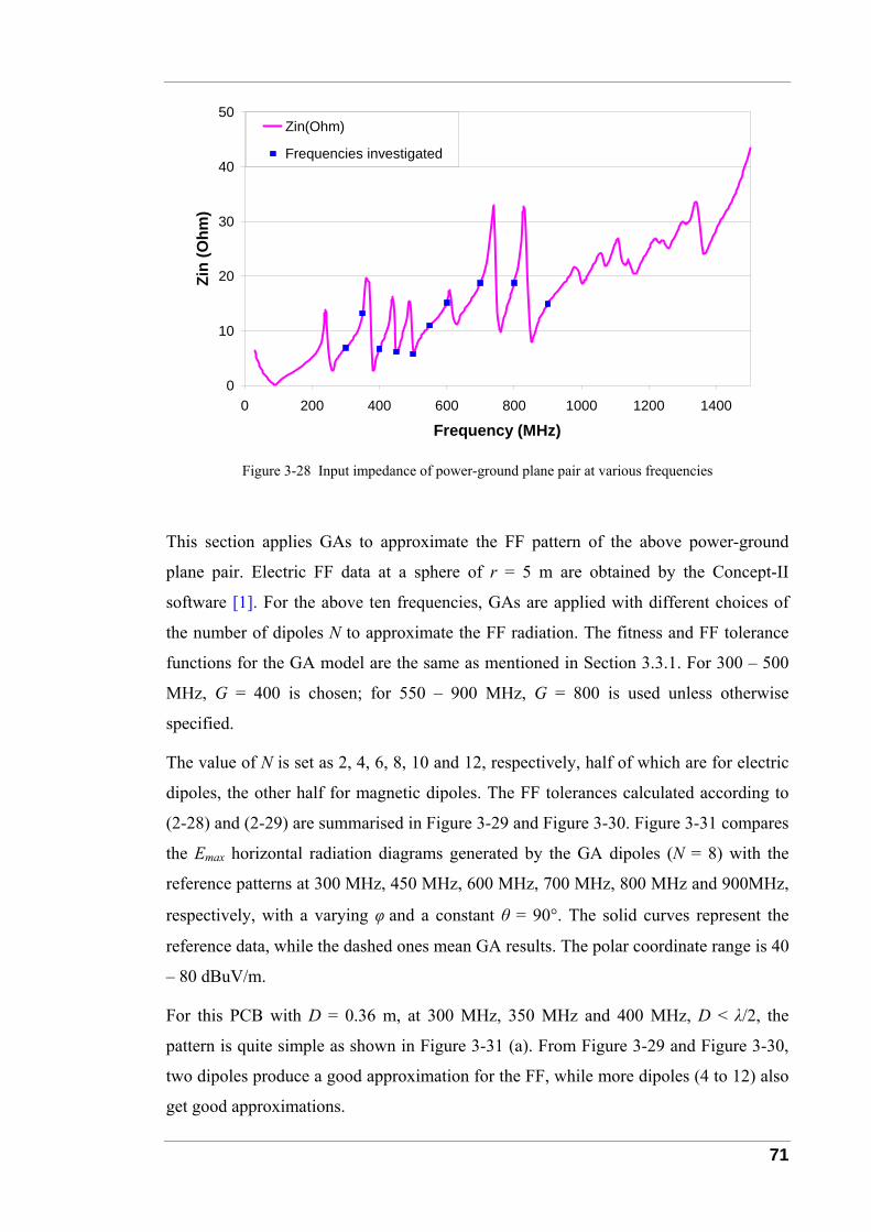
71

0

10

20

30

40

50

0 200 400 600 800 1000 1200 1400

Frequency (MHz)

Zin

(Ohm

)

Zin(Ohm)

Frequencies investigated

Figure 3-28 Input impedance of power-ground plane pair at various frequencies

This section applies GAs to approximate the FF pattern of the above power-ground

plane pair. Electric FF data at a sphere of r = 5 m are obtained by the Concept-II

software [1]. For the above ten frequencies, GAs are applied with different choices of

the number of dipoles N to approximate the FF radiation. The fitness and FF tolerance

functions for the GA model are the same as mentioned in Section 3.3.1. For 300 – 500

MHz, G = 400 is chosen; for 550 – 900 MHz, G = 800 is used unless otherwise

specified.

The value of N is set as 2, 4, 6, 8, 10 and 12, respectively, half of which are for electric

dipoles, the other half for magnetic dipoles. The FF tolerances calculated according to

(2-28) and (2-29) are summarised in Figure 3-29 and Figure 3-30. Figure 3-31 compares

the Emax horizontal radiation diagrams generated by the GA dipoles (N = 8) with the

reference patterns at 300 MHz, 450 MHz, 600 MHz, 700 MHz, 800 MHz and 900MHz,

respectively, with a varying φ and a constant θ = 90°. The solid curves represent the

reference data, while the dashed ones mean GA results. The polar coordinate range is 40

– 80 dBuV/m.

For this PCB with D = 0.36 m, at 300 MHz, 350 MHz and 400 MHz, D < λ/2, the

pattern is quite simple as shown in Figure 3-31 (a). From Figure 3-29 and Figure 3-30,

two dipoles produce a good approximation for the FF, while more dipoles (4 to 12) also

get good approximations.

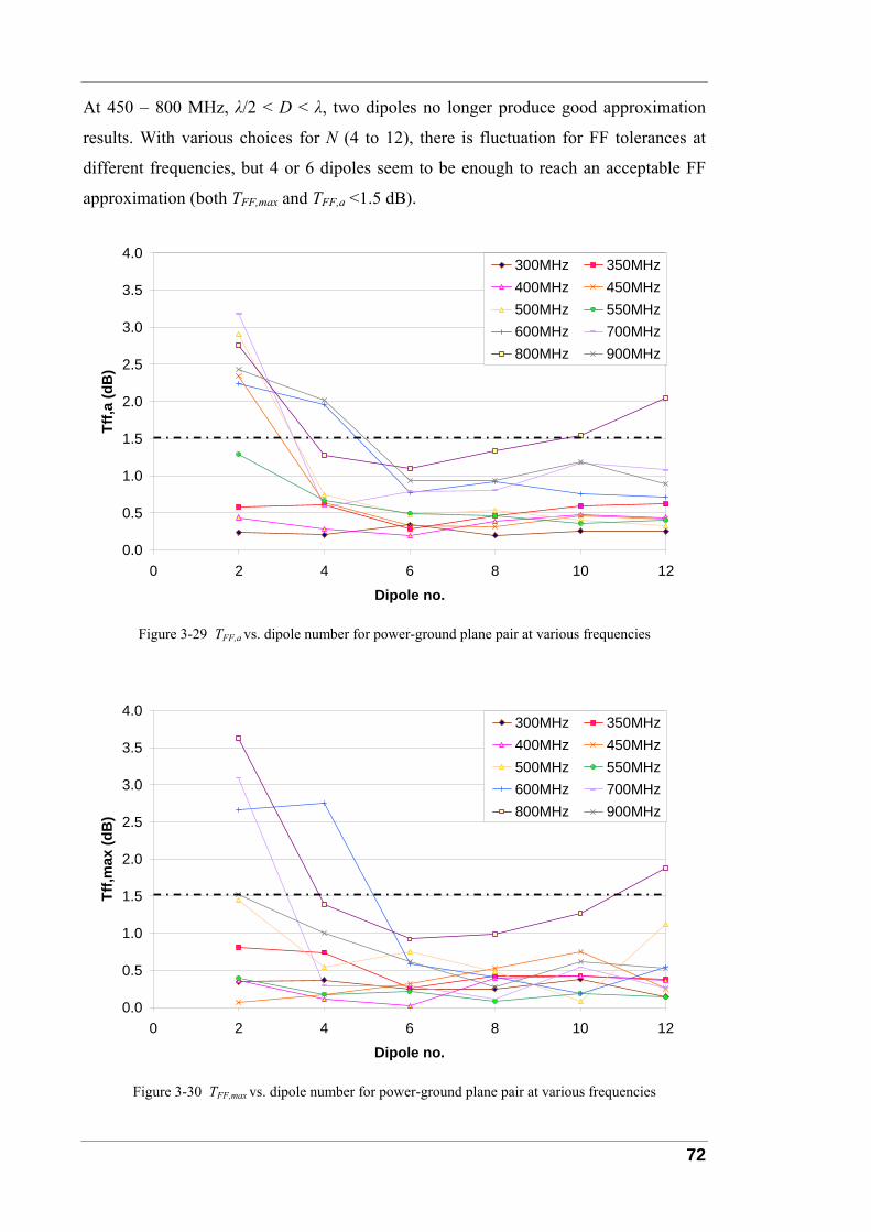
72

At 450 – 800 MHz, λ/2 < D < λ, two dipoles no longer produce good approximation

results. With various choices for N (4 to 12), there is fluctuation for FF tolerances at

different frequencies, but 4 or 6 dipoles seem to be enough to reach an acceptable FF

approximation (both TFF,max and TFF,a <1.5 dB).

0.0

0.5

1.0

1.5

2.0

2.5

3.0

3.5

4.0

0 2 4 6 8 10 12

Dipole no.

Tff,a

(dB

)

300MHz 350MHz400MHz 450MHz500MHz 550MHz600MHz 700MHz800MHz 900MHz

Figure 3-29 TFF,a vs. dipole number for power-ground plane pair at various frequencies

0.0

0.5

1.0

1.5

2.0

2.5

3.0

3.5

4.0

0 2 4 6 8 10 12

Dipole no.

Tff,m

ax (d

B)

300MHz 350MHz400MHz 450MHz500MHz 550MHz600MHz 700MHz800MHz 900MHz

Figure 3-30 TFF,max vs. dipole number for power-ground plane pair at various frequencies

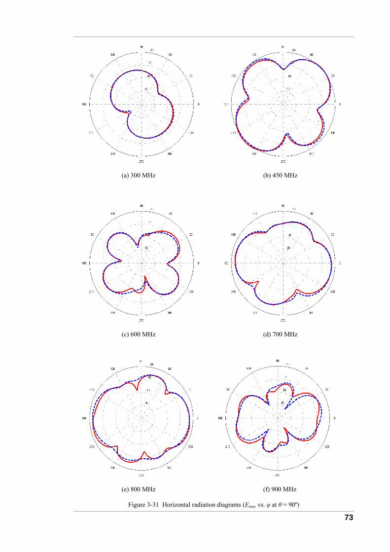
73

(a) 300 MHz (b) 450 MHz

(c) 600 MHz (d) 700 MHz

(e) 800 MHz (f) 900 MHz

Figure 3-31 Horizontal radiation diagrams (Emax vs. φ at θ = 90º)

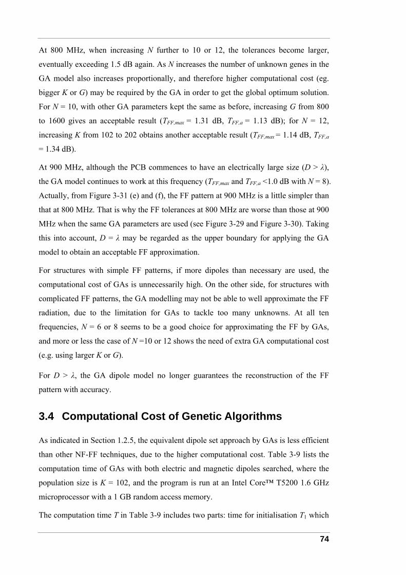
74

At 800 MHz, when increasing N further to 10 or 12, the tolerances become larger,

eventually exceeding 1.5 dB again. As N increases the number of unknown genes in the

GA model also increases proportionally, and therefore higher computational cost (eg.

bigger K or G) may be required by the GA in order to get the global optimum solution.

For N = 10, with other GA parameters kept the same as before, increasing G from 800

to 1600 gives an acceptable result (TFF,max = 1.31 dB, TFF,a = 1.13 dB); for N = 12,

increasing K from 102 to 202 obtains another acceptable result (TFF,max = 1.14 dB, TFF,a

= 1.34 dB).

At 900 MHz, although the PCB commences to have an electrically large size (D > λ),

the GA model continues to work at this frequency (TFF,max and TFF,a <1.0 dB with N = 8).

Actually, from Figure 3-31 (e) and (f), the FF pattern at 900 MHz is a little simpler than

that at 800 MHz. That is why the FF tolerances at 800 MHz are worse than those at 900

MHz when the same GA parameters are used (see Figure 3-29 and Figure 3-30). Taking

this into account, D = λ may be regarded as the upper boundary for applying the GA

model to obtain an acceptable FF approximation.

For structures with simple FF patterns, if more dipoles than necessary are used, the

computational cost of GAs is unnecessarily high. On the other side, for structures with

complicated FF patterns, the GA modelling may not be able to well approximate the FF

radiation, due to the limitation for GAs to tackle too many unknowns. At all ten

frequencies, N = 6 or 8 seems to be a good choice for approximating the FF by GAs,

and more or less the case of N =10 or 12 shows the need of extra GA computational cost

(e.g. using larger K or G).

For D > λ, the GA dipole model no longer guarantees the reconstruction of the FF

pattern with accuracy.

3.4 Computational Cost of Genetic Algorithms

As indicated in Section 1.2.5, the equivalent dipole set approach by GAs is less efficient

than other NF-FF techniques, due to the higher computational cost. Table 3-9 lists the

computation time of GAs with both electric and magnetic dipoles searched, where the

population size is K = 102, and the program is run at an Intel Core™ T5200 1.6 GHz

microprocessor with a 1 GB random access memory.

The computation time T in Table 3-9 includes two parts: time for initialisation T1 which

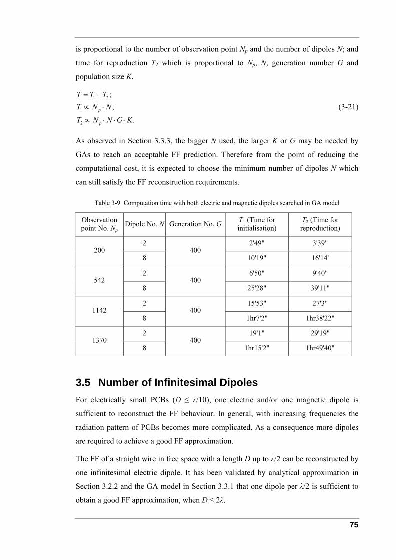
75

is proportional to the number of observation point Np and the number of dipoles N; and

time for reproduction T2 which is proportional to Np, N, generation number G and

population size K.

1 2

1

2

;;

.p

p

T T TT N N

T N N G K

= +∝ ⋅

∝ ⋅ ⋅ ⋅

(3-21)

As observed in Section 3.3.3, the bigger N used, the larger K or G may be needed by

GAs to reach an acceptable FF prediction. Therefore from the point of reducing the

computational cost, it is expected to choose the minimum number of dipoles N which

can still satisfy the FF reconstruction requirements.

Table 3-9 Computation time with both electric and magnetic dipoles searched in GA model

Observation point No. Np

Dipole No. N Generation No. G T1 (Time for initialisation)

T2 (Time for reproduction)

2 2'49" 3'39" 200

8 400

10'19" 16'14'

2 6'50" 9'40" 542

8 400

25'28" 39'11"

2 15'53" 27'3" 1142

8 400

1hr7'2" 1hr38'22"

2 19'1" 29'19" 1370

8 400

1hr15'2" 1hr49'40"

3.5 Number of Infinitesimal Dipoles For electrically small PCBs (D ≤ λ/10), one electric and/or one magnetic dipole is

sufficient to reconstruct the FF behaviour. In general, with increasing frequencies the

radiation pattern of PCBs becomes more complicated. As a consequence more dipoles

are required to achieve a good FF approximation.

The FF of a straight wire in free space with a length D up to λ/2 can be reconstructed by

one infinitesimal electric dipole. It has been validated by analytical approximation in

Section 3.2.2 and the GA model in Section 3.3.1 that one dipole per λ/2 is sufficient to

obtain a good FF approximation, when D ≤ 2λ.

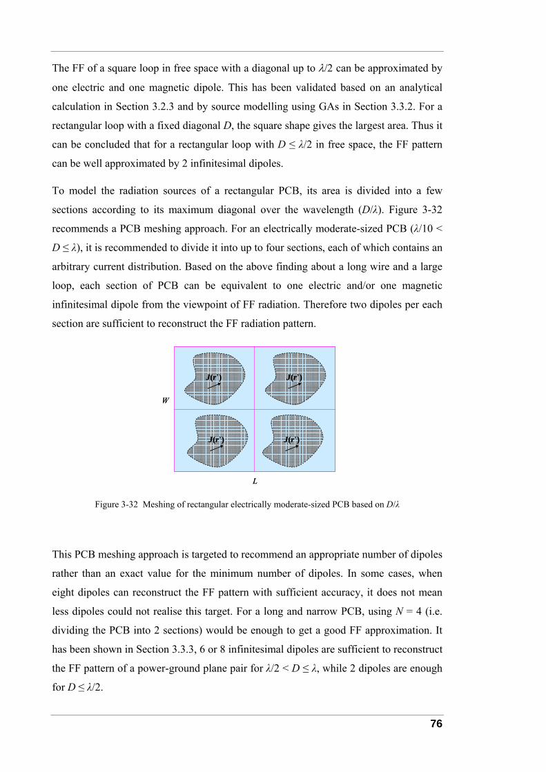
76

The FF of a square loop in free space with a diagonal up to λ/2 can be approximated by

one electric and one magnetic dipole. This has been validated based on an analytical

calculation in Section 3.2.3 and by source modelling using GAs in Section 3.3.2. For a

rectangular loop with a fixed diagonal D, the square shape gives the largest area. Thus it

can be concluded that for a rectangular loop with D ≤ λ/2 in free space, the FF pattern

can be well approximated by 2 infinitesimal dipoles.

To model the radiation sources of a rectangular PCB, its area is divided into a few

sections according to its maximum diagonal over the wavelength (D/λ). Figure 3-32

recommends a PCB meshing approach. For an electrically moderate-sized PCB (λ/10 <

D ≤ λ), it is recommended to divide it into up to four sections, each of which contains an

arbitrary current distribution. Based on the above finding about a long wire and a large

loop, each section of PCB can be equivalent to one electric and/or one magnetic

infinitesimal dipole from the viewpoint of FF radiation. Therefore two dipoles per each

section are sufficient to reconstruct the FF radiation pattern.

L

W

J(r’)

J(r’)

J(r’)

J(r’)

L

W

J(r’)J(r’)

J(r’)J(r’)

J(r’)J(r’)

J(r’)J(r’)

Figure 3-32 Meshing of rectangular electrically moderate-sized PCB based on D/λ

This PCB meshing approach is targeted to recommend an appropriate number of dipoles

rather than an exact value for the minimum number of dipoles. In some cases, when

eight dipoles can reconstruct the FF pattern with sufficient accuracy, it does not mean

less dipoles could not realise this target. For a long and narrow PCB, using N = 4 (i.e.

dividing the PCB into 2 sections) would be enough to get a good FF approximation. It

has been shown in Section 3.3.3, 6 or 8 infinitesimal dipoles are sufficient to reconstruct

the FF pattern of a power-ground plane pair for λ/2 < D ≤ λ, while 2 dipoles are enough

for D ≤ λ/2.

77

In the PCB design for high frequency circuits, a lot of radiation sources exist, such as

antennas in mobile devices, wire leads with high pulse voltage and high frequency

current loops. Unlike the examples with symmetrical structures shown in Section 3.3, a

realistic PCB design usually brings about more asymmetry for electromagnetic radiation,

due to the existence of finite-sized ground planes, ground plane partitions etc. In general,

asymmetrical FF patterns need more dipoles to reconstruct compared to symmetrical

ones. Therefore it is recommended to use 8 dipoles to approximate the FF of PCBs with

a size in the range of λ/10 < D ≤ λ/2.

In summary, using the GA model to predict FF radiation for PCBs with a maximum size

D, the number of infinitesimal dipoles N is recommended to be as follows:

2, for ;10

8, for .10

N D

N D

λ

λ λ

= ≤

= < ≤ (3-22)

For D > λ, the GA model does not guarantee to find the global optimum solution for this

NF-FF conversion.

78

4 Near Field Data Sampling Approaches

Chapter 2 built a fundamental GA model for NF-FF conversion, where the optimum

fitness definition was found to be 1/TNF,a based on (2-19). The FF tolerances TFF,a and

TFF,max were defined in (2-28) and (2-29), respectively. The correlation between NF and

FF tolerances ( ), ,max,NF a FFCorr T T and ( ), ,,NF a FF aCorr T T based on (2-30) was discussed.

These definitions will be adopted for the remaining modelling in this thesis.

The aim of this chapter is to investigate how NF data should be sampled as the input of

the GA model for the NF-FF conversion, such as where to locate NF sampling points,

what type of data to collect, how to choose the plane coverage angle when data on open

planes are collected (see Section 4.5), how many points to observe, how many planes to

choose, and how close these planes should be. Meanwhile, the necessary number of

infinitesimal dipoles mentioned in Section 3.5 is validated.

This chapter evaluates NF data sampling approaches for a 90 mm × 60 mm PCB with a

finite ground plane, with the GA described in Chapter 2. At observation points evenly

spaced in one or more square grids, simulated magnetic NF magnitudes are input into

the GA model. Simulated FF data at a sphere of 3 m radius are used to calculate FF

tolerances. As mentioned in Section 3.3, for each case the GA model runs 5 times. With

5 GA runs, the minimum, average, maximum and range (Δ) values of FF tolerances are

recorded. The lower the minimum, the better the optimum solution is obtained. The

lower the average and Δ, the more stable solution is achieved and the better the GA

repeatability is.

Outline

This chapter comprises 11 sections. Section 4.1 introduces the basic configuration of the

example PCB. Section 4.2 describes the definition of reactive and radiating NF regions,

and introduces a list of 12 NF sampling cases to be investigated in this chapter. Section

4.3 considers the dipole location boundary taking into account the asymmetrical field

pattern of the PCB. Section 4.4 compares the NF data sampling in radiating NF and

reactive NF regions for the FF radiation prediction, and Section 4.5 considers the NF

plane coverage angle. Section 4.6 compares the GA results from different NF data

types, such as three components of magnetic field peak magnitudes on open planes, and

tangential-only magnetic field components on either open planes or closed surfaces.

79

Section 4.7 determines how many points should be sampled, and Section 4.8 discusses

how many NF planes are to be observed. Section 4.9 analyses the NF-FF conversion

results with various choices for the number of dipoles. Section 4.10 discusses the

dynamic data range, and Section 4.11 summarises the whole chapter.

Contributions

The main contributions of this chapter include:

1) In order to predict FF radiation of a PCB by NF data based on the GA model, it

is important to have a location margin for the equivalent dipole set which is a

little bigger than the PCB physical size. This methodology may help reconstruct

some characteristics of the radiation PCB, such as radiation asymmetry (due to

finite ground plane, ground plane splitting etc). This chapter concludes 5 mm as

the optimum margin for this 90 mm × 60 mm PCB.

2) The definitions of reactive NF, radiating NF and FF regions are clearly defined.

In examining the PCB, it is concluded that the NF data collected from the

radiating NF region are better for FF prediction than those from the reactive NF

region.

3) If NF sampling is done on a closed surface, tangential magnetic NF components

may be sufficient to determine FF radiation. However, if NF sampling is done

on open surfaces, the additional availability of normal magnetic field

components improves the results. Furthermore, for planar sampling on an open

surface, the plane coverage angle θ is influential for obtaining a stable NF-FF

conversion result (see Section 4.5). It is observed that θ > 60° results in a good

repeatability for the FF prediction.

4) Number of observation points should be more than the number of unknown

genes to obtain a stable GA result. For a GA model with dipole number N = 8

(64 unknowns), it is suggested that 100 observation points per sampling plane

should be chosen, and the sampling spacing on the plane should be less than the

half wavelength (λ/2).

5) With regard to the number of sampling planes on each side of the x-y plane, it is

shown that FF prediction can be improved using 2 planes instead of 1 plane,

however, the same cannot be said using 3 planes. For the distance between two

sampling planes, although there is no strict rule from the Nyquist sampling

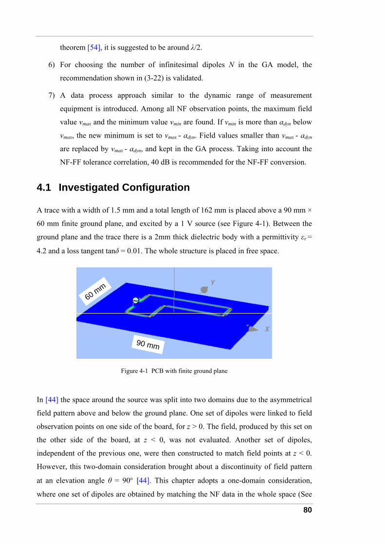
80

theorem [54], it is suggested to be around λ/2.

6) For choosing the number of infinitesimal dipoles N in the GA model, the

recommendation shown in (3-22) is validated.

7) A data process approach similar to the dynamic range of measurement

equipment is introduced. Among all NF observation points, the maximum field

value vmax and the minimum value vmin are found. If vmin is more than adyn below

vmax, the new minimum is set to vmax - adyn. Field values smaller than vmax - adyn

are replaced by vmax - adyn, and kept in the GA process. Taking into account the

NF-FF tolerance correlation, 40 dB is recommended for the NF-FF conversion.

4.1 Investigated Configuration

A trace with a width of 1.5 mm and a total length of 162 mm is placed above a 90 mm ×

60 mm finite ground plane, and excited by a 1 V source (see Figure 4-1). Between the

ground plane and the trace there is a 2mm thick dielectric body with a permittivity εr =

4.2 and a loss tangent tanδ = 0.01. The whole structure is placed in free space.

60 mm

90 mm

~60 mm

90 mm

~

Figure 4-1 PCB with finite ground plane

In [44] the space around the source was split into two domains due to the asymmetrical

field pattern above and below the ground plane. One set of dipoles were linked to field

observation points on one side of the board, for z > 0. The field, produced by this set on

the other side of the board, at z < 0, was not evaluated. Another set of dipoles,

independent of the previous one, were then constructed to match field points at z < 0.

However, this two-domain consideration brought about a discontinuity of field pattern

at an elevation angle θ = 90° [44]. This chapter adopts a one-domain consideration,

where one set of dipoles are obtained by matching the NF data in the whole space (See

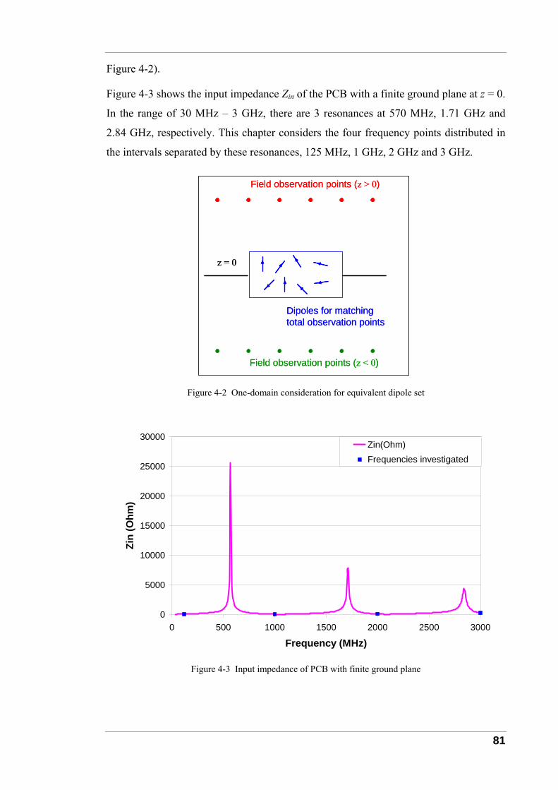
81

Figure 4-2).

Figure 4-3 shows the input impedance Zin of the PCB with a finite ground plane at z = 0.

In the range of 30 MHz – 3 GHz, there are 3 resonances at 570 MHz, 1.71 GHz and

2.84 GHz, respectively. This chapter considers the four frequency points distributed in

the intervals separated by these resonances, 125 MHz, 1 GHz, 2 GHz and 3 GHz.

z = 0

Dipoles for matchingtotal observation points

Field observation points (z > 0)

Field observation points (z < 0)

z = 0

Dipoles for matchingtotal observation points

Field observation points (z > 0)

Field observation points (z < 0)

Figure 4-2 One-domain consideration for equivalent dipole set

0

5000

10000

15000

20000

25000

30000

0 500 1000 1500 2000 2500 3000

Frequency (MHz)

Zin

(Ohm

)

Zin(Ohm)Frequencies investigated

Figure 4-3 Input impedance of PCB with finite ground plane

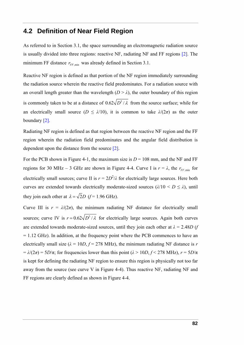
82

4.2 Definition of Near Field Region

As referred to in Section 3.1, the space surrounding an electromagnetic radiation source

is usually divided into three regions: reactive NF, radiating NF and FF regions [2]. The

minimum FF distance ,minFFr was already defined in Section 3.1.

Reactive NF region is defined as that portion of the NF region immediately surrounding

the radiation source wherein the reactive field predominates. For a radiation source with

an overall length greater than the wavelength (D > λ), the outer boundary of this region

is commonly taken to be at a distance of 30.62 /D λ from the source surface; while for

an electrically small source (D ≤ λ/10), it is common to take λ/(2π) as the outer

boundary [2].

Radiating NF region is defined as that region between the reactive NF region and the FF

region wherein the radiation field predominates and the angular field distribution is

dependent upon the distance from the source [2].

For the PCB shown in Figure 4-1, the maximum size is D = 108 mm, and the NF and FF

regions for 30 MHz – 3 GHz are shown in Figure 4-4. Curve I is r = λ, the ,minFFr for

electrically small sources; curve II is r = 2D2/λ for electrically large sources. Here both

curves are extended towards electrically moderate-sized sources (λ/10 < D ≤ λ), until

they join each other at 2Dλ = (f = 1.96 GHz).

Curve III is r = λ/(2π), the minimum radiating NF distance for electrically small

sources; curve IV is 30.62 /r D λ= for electrically large sources. Again both curves

are extended towards moderate-sized sources, until they join each other at λ = 2.48D (f

= 1.12 GHz). In addition, at the frequency point where the PCB commences to have an

electrically small size (λ = 10D, f = 278 MHz), the minimum radiating NF distance is r

= λ/(2π) = 5D/π; for frequencies lower than this point (λ > 10D, f < 278 MHz), r = 5D/π

is kept for defining the radiating NF region to ensure this region is physically not too far

away from the source (see curve V in Figure 4-4). Thus reactive NF, radiating NF and

FF regions are clearly defined as shown in Figure 4-4.

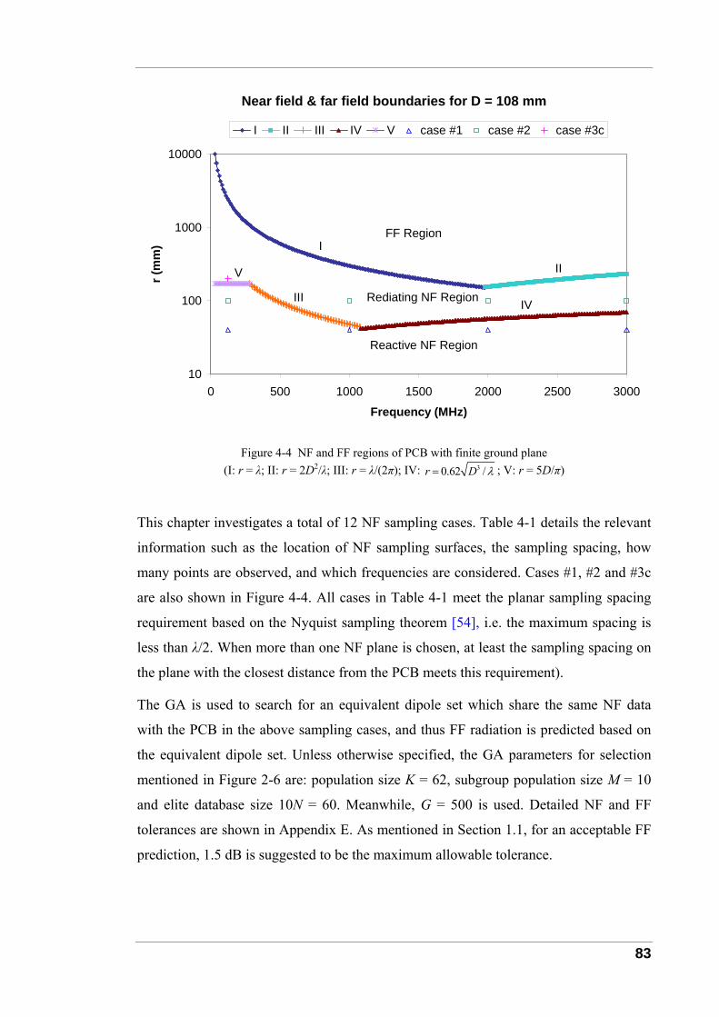
83

Near field & far field boundaries for D = 108 mm

10

100

1000

10000

0 500 1000 1500 2000 2500 3000

Frequency (MHz)

r (m

m)

I II III IV V case #1 case #2 case #3c

FF Region

Rediating NF Region

Reactive NF Region

I

V

IVIII

II

Figure 4-4 NF and FF regions of PCB with finite ground plane (I: r = λ; II: r = 2D2/λ; III: r = λ/(2π); IV: 30.62 /r D λ= ; V: r = 5D/π)

This chapter investigates a total of 12 NF sampling cases. Table 4-1 details the relevant

information such as the location of NF sampling surfaces, the sampling spacing, how

many points are observed, and which frequencies are considered. Cases #1, #2 and #3c

are also shown in Figure 4-4. All cases in Table 4-1 meet the planar sampling spacing

requirement based on the Nyquist sampling theorem [54], i.e. the maximum spacing is

less than λ/2. When more than one NF plane is chosen, at least the sampling spacing on

the plane with the closest distance from the PCB meets this requirement).

The GA is used to search for an equivalent dipole set which share the same NF data

with the PCB in the above sampling cases, and thus FF radiation is predicted based on

the equivalent dipole set. Unless otherwise specified, the GA parameters for selection

mentioned in Figure 2-6 are: population size K = 62, subgroup population size M = 10

and elite database size 10N = 60. Meanwhile, G = 500 is used. Detailed NF and FF

tolerances are shown in Appendix E. As mentioned in Section 1.1, for an acceptable FF

prediction, 1.5 dB is suggested to be the maximum allowable tolerance.

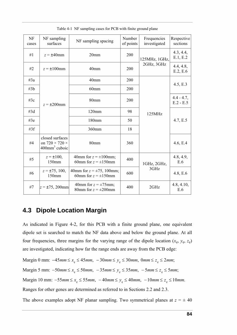
84

Table 4-1 NF sampling cases for PCB with finite ground plane

NF cases

NF sampling surfaces NF sampling spacing Number

of pointsFrequencies investigated

Respective sections

#1 z = ±40mm 20mm 200 4.3, 4.4, E.1, E.2

#2 z = ±100mm 40mm 200

125MHz, 1GHz, 2GHz, 3GHz 4.4, 4.8,

E.2, E.6

#3a 40mm 200

#3b 60mm 200 4.5, E.3

#3c 80mm 200 4.4 - 4.7, E.2 - E.5

#3d 120mm 98

#3e 180mm 50

#3f

z = ±200mm

360mm 18

4.7, E.5

#4 closed surfaces on 720 × 720 × 400mm3 cuboic

80mm 360

125MHz

4.6, E.4

#5 z = ±100, 150mm

40mm for z = ±100mm; 60mm for z = ±150mm 400 4.8, 4.9,

E.6

#6 z = ±75, 100, 150mm

40mm for z = ±75, 100mm; 60mm for z = ±150mm 600

1GHz, 2GHz, 3GHz

4.8, E.6

#7 z = ±75, 200mm 40mm for z = ±75mm; 80mm for z = ±200mm 400 2GHz 4.8, 4.10,

E.6

4.3 Dipole Location Margin

As indicated in Figure 4-2, for this PCB with a finite ground plane, one equivalent

dipole set is searched to match the NF data above and below the ground plane. At all

four frequencies, three margins for the varying range of the dipole location (xq, yq, zq)

are investigated, indicating how far the range ends are away from the PCB edge:

Margin 0 mm: 45 45 , 30 30 , 0 2 ;q q qmm x mm mm y mm mm z mm− ≤ ≤ − ≤ ≤ ≤ ≤

Margin 5 mm: 50 50 , 35 35 , 5 5 ;q q qmm x mm mm y mm mm z mm− ≤ ≤ − ≤ ≤ − ≤ ≤

Margin 10 mm: 55 55 , 40 40 , 10 10 .q q qmm x mm mm y mm mm z mm− ≤ ≤ − ≤ ≤ − ≤ ≤

Ranges for other genes are determined as referred to in Sections 2.2 and 2.3.

The above examples adopt NF planar sampling. Two symmetrical planes at z = ± 40

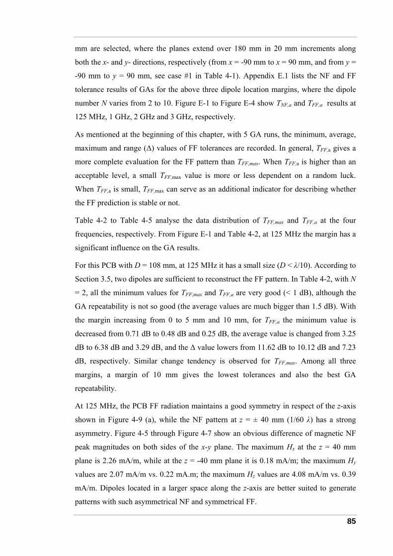
85

mm are selected, where the planes extend over 180 mm in 20 mm increments along

both the x- and y- directions, respectively (from x = -90 mm to x = 90 mm, and from y =

-90 mm to y = 90 mm, see case #1 in Table 4-1). Appendix E.1 lists the NF and FF

tolerance results of GAs for the above three dipole location margins, where the dipole

number N varies from 2 to 10. Figure E-1 to Figure E-4 show TNF,a and TFF,a results at

125 MHz, 1 GHz, 2 GHz and 3 GHz, respectively.

As mentioned at the beginning of this chapter, with 5 GA runs, the minimum, average,

maximum and range (Δ) values of FF tolerances are recorded. In general, TFF,a gives a

more complete evaluation for the FF pattern than TFF,max. When TFF,a is higher than an

acceptable level, a small TFF,max value is more or less dependent on a random luck.

When TFF,a is small, TFF,max can serve as an additional indicator for describing whether

the FF prediction is stable or not.

Table 4-2 to Table 4-5 analyse the data distribution of TFF,max and TFF,a at the four

frequencies, respectively. From Figure E-1 and Table 4-2, at 125 MHz the margin has a

significant influence on the GA results.

For this PCB with D = 108 mm, at 125 MHz it has a small size (D < λ/10). According to

Section 3.5, two dipoles are sufficient to reconstruct the FF pattern. In Table 4-2, with N

= 2, all the minimum values for TFF,max and TFF,a are very good (< 1 dB), although the

GA repeatability is not so good (the average values are much bigger than 1.5 dB). With

the margin increasing from 0 to 5 mm and 10 mm, for TFF,a the minimum value is

decreased from 0.71 dB to 0.48 dB and 0.25 dB, the average value is changed from 3.25

dB to 6.38 dB and 3.29 dB, and the Δ value lowers from 11.62 dB to 10.12 dB and 7.23

dB, respectively. Similar change tendency is observed for TFF,max. Among all three

margins, a margin of 10 mm gives the lowest tolerances and also the best GA

repeatability.

At 125 MHz, the PCB FF radiation maintains a good symmetry in respect of the z-axis

shown in Figure 4-9 (a), while the NF pattern at z = ± 40 mm (1/60 λ) has a strong

asymmetry. Figure 4-5 through Figure 4-7 show an obvious difference of magnetic NF

peak magnitudes on both sides of the x-y plane. The maximum Hx at the z = 40 mm

plane is 2.26 mA/m, while at the z = -40 mm plane it is 0.18 mA/m; the maximum Hy

values are 2.07 mA/m vs. 0.22 mA.m; the maximum Hz values are 4.08 mA/m vs. 0.39

mA/m. Dipoles located in a larger space along the z-axis are better suited to generate

patterns with such asymmetrical NF and symmetrical FF.

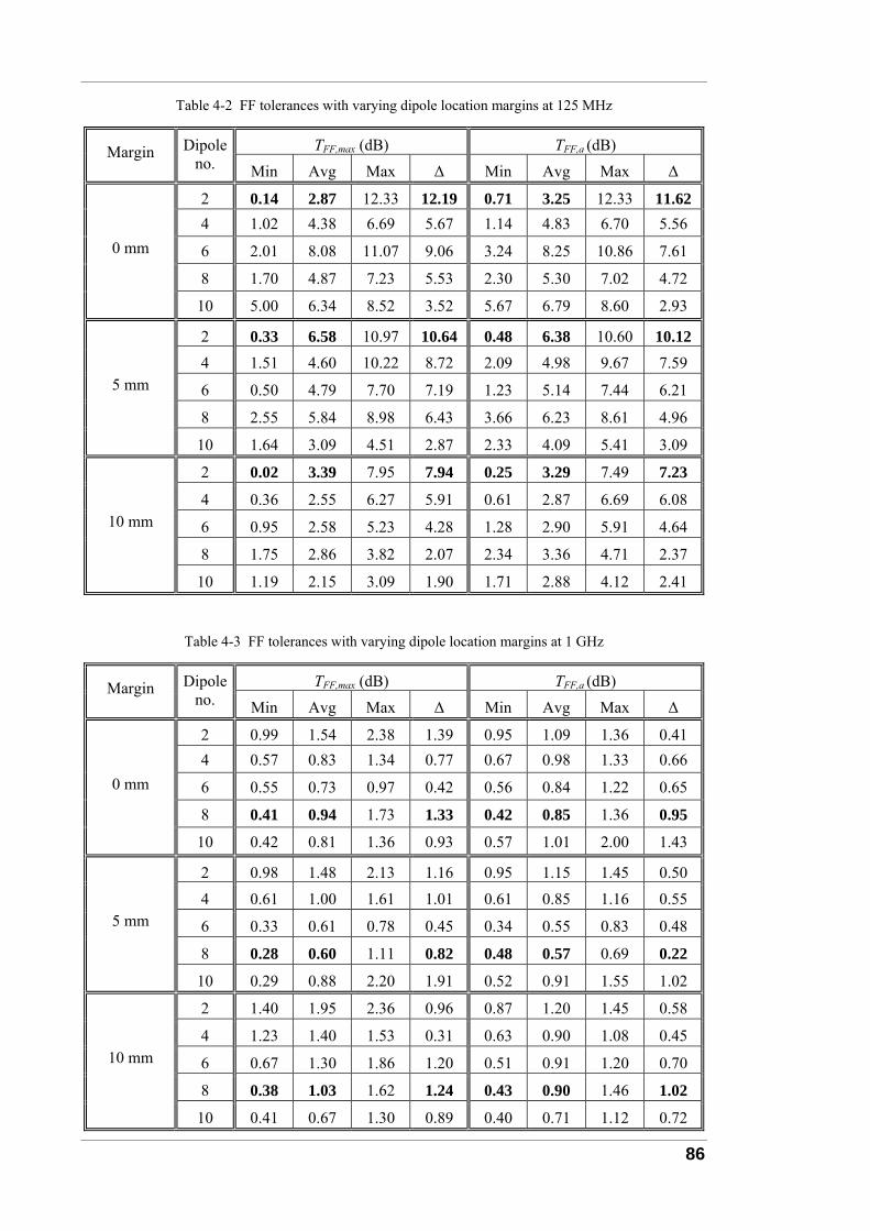
86

Table 4-2 FF tolerances with varying dipole location margins at 125 MHz

TFF,max (dB) TFF,a (dB) Margin Dipole no. Min Avg Max Δ Min Avg Max Δ

2 0.14 2.87 12.33 12.19 0.71 3.25 12.33 11.62 4 1.02 4.38 6.69 5.67 1.14 4.83 6.70 5.56

6 2.01 8.08 11.07 9.06 3.24 8.25 10.86 7.61

8 1.70 4.87 7.23 5.53 2.30 5.30 7.02 4.72

0 mm

10 5.00 6.34 8.52 3.52 5.67 6.79 8.60 2.93

2 0.33 6.58 10.97 10.64 0.48 6.38 10.60 10.12 4 1.51 4.60 10.22 8.72 2.09 4.98 9.67 7.59

6 0.50 4.79 7.70 7.19 1.23 5.14 7.44 6.21

8 2.55 5.84 8.98 6.43 3.66 6.23 8.61 4.96

5 mm

10 1.64 3.09 4.51 2.87 2.33 4.09 5.41 3.09

2 0.02 3.39 7.95 7.94 0.25 3.29 7.49 7.23

4 0.36 2.55 6.27 5.91 0.61 2.87 6.69 6.08

6 0.95 2.58 5.23 4.28 1.28 2.90 5.91 4.64

8 1.75 2.86 3.82 2.07 2.34 3.36 4.71 2.37

10 mm

10 1.19 2.15 3.09 1.90 1.71 2.88 4.12 2.41

Table 4-3 FF tolerances with varying dipole location margins at 1 GHz

TFF,max (dB) TFF,a (dB) Margin Dipole no. Min Avg Max Δ Min Avg Max Δ

2 0.99 1.54 2.38 1.39 0.95 1.09 1.36 0.41 4 0.57 0.83 1.34 0.77 0.67 0.98 1.33 0.66

6 0.55 0.73 0.97 0.42 0.56 0.84 1.22 0.65

8 0.41 0.94 1.73 1.33 0.42 0.85 1.36 0.95

0 mm

10 0.42 0.81 1.36 0.93 0.57 1.01 2.00 1.43

2 0.98 1.48 2.13 1.16 0.95 1.15 1.45 0.50 4 0.61 1.00 1.61 1.01 0.61 0.85 1.16 0.55

6 0.33 0.61 0.78 0.45 0.34 0.55 0.83 0.48

8 0.28 0.60 1.11 0.82 0.48 0.57 0.69 0.22

5 mm

10 0.29 0.88 2.20 1.91 0.52 0.91 1.55 1.02

2 1.40 1.95 2.36 0.96 0.87 1.20 1.45 0.58

4 1.23 1.40 1.53 0.31 0.63 0.90 1.08 0.45

6 0.67 1.30 1.86 1.20 0.51 0.91 1.20 0.70

8 0.38 1.03 1.62 1.24 0.43 0.90 1.46 1.02

10 mm

10 0.41 0.67 1.30 0.89 0.40 0.71 1.12 0.72

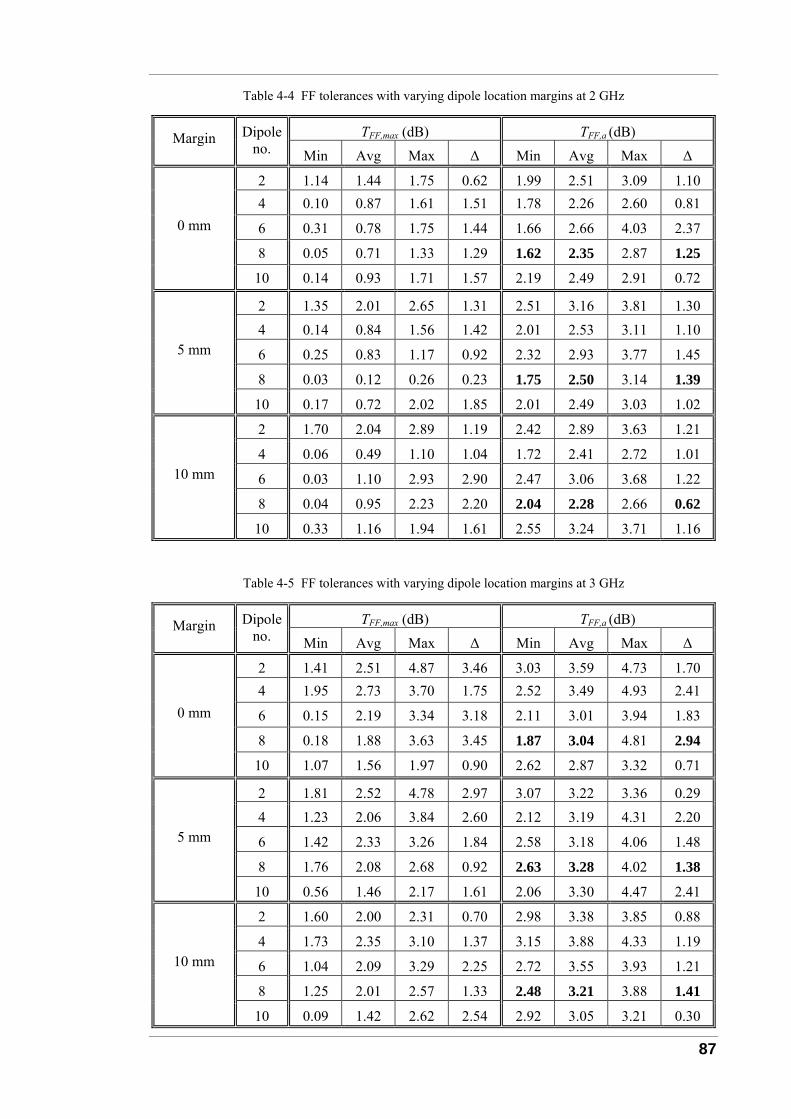
87

Table 4-4 FF tolerances with varying dipole location margins at 2 GHz

TFF,max (dB) TFF,a (dB) Margin Dipole no. Min Avg Max Δ Min Avg Max Δ

2 1.14 1.44 1.75 0.62 1.99 2.51 3.09 1.10 4 0.10 0.87 1.61 1.51 1.78 2.26 2.60 0.81

6 0.31 0.78 1.75 1.44 1.66 2.66 4.03 2.37

8 0.05 0.71 1.33 1.29 1.62 2.35 2.87 1.25

0 mm

10 0.14 0.93 1.71 1.57 2.19 2.49 2.91 0.72

2 1.35 2.01 2.65 1.31 2.51 3.16 3.81 1.30 4 0.14 0.84 1.56 1.42 2.01 2.53 3.11 1.10

6 0.25 0.83 1.17 0.92 2.32 2.93 3.77 1.45

8 0.03 0.12 0.26 0.23 1.75 2.50 3.14 1.39

5 mm

10 0.17 0.72 2.02 1.85 2.01 2.49 3.03 1.02

2 1.70 2.04 2.89 1.19 2.42 2.89 3.63 1.21

4 0.06 0.49 1.10 1.04 1.72 2.41 2.72 1.01

6 0.03 1.10 2.93 2.90 2.47 3.06 3.68 1.22

8 0.04 0.95 2.23 2.20 2.04 2.28 2.66 0.62

10 mm

10 0.33 1.16 1.94 1.61 2.55 3.24 3.71 1.16

Table 4-5 FF tolerances with varying dipole location margins at 3 GHz

TFF,max (dB) TFF,a (dB) Margin Dipole no. Min Avg Max Δ Min Avg Max Δ

2 1.41 2.51 4.87 3.46 3.03 3.59 4.73 1.70 4 1.95 2.73 3.70 1.75 2.52 3.49 4.93 2.41

6 0.15 2.19 3.34 3.18 2.11 3.01 3.94 1.83

8 0.18 1.88 3.63 3.45 1.87 3.04 4.81 2.94

0 mm

10 1.07 1.56 1.97 0.90 2.62 2.87 3.32 0.71

2 1.81 2.52 4.78 2.97 3.07 3.22 3.36 0.29 4 1.23 2.06 3.84 2.60 2.12 3.19 4.31 2.20

6 1.42 2.33 3.26 1.84 2.58 3.18 4.06 1.48

8 1.76 2.08 2.68 0.92 2.63 3.28 4.02 1.38

5 mm

10 0.56 1.46 2.17 1.61 2.06 3.30 4.47 2.41

2 1.60 2.00 2.31 0.70 2.98 3.38 3.85 0.88

4 1.73 2.35 3.10 1.37 3.15 3.88 4.33 1.19

6 1.04 2.09 3.29 2.25 2.72 3.55 3.93 1.21

8 1.25 2.01 2.57 1.33 2.48 3.21 3.88 1.41

10 mm

10 0.09 1.42 2.62 2.54 2.92 3.05 3.21 0.30

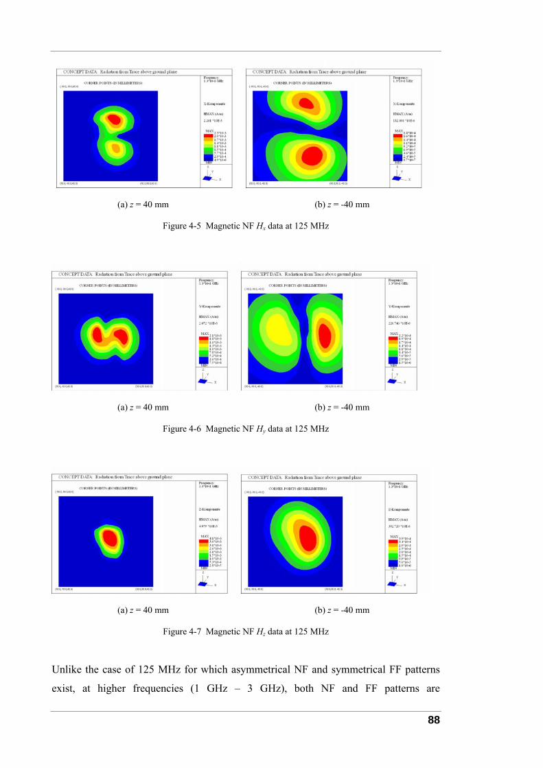
88

(a) z = 40 mm (b) z = -40 mm

Figure 4-5 Magnetic NF Hx data at 125 MHz

(a) z = 40 mm (b) z = -40 mm

Figure 4-6 Magnetic NF Hy data at 125 MHz

(a) z = 40 mm (b) z = -40 mm

Figure 4-7 Magnetic NF Hz data at 125 MHz

Unlike the case of 125 MHz for which asymmetrical NF and symmetrical FF patterns

exist, at higher frequencies (1 GHz – 3 GHz), both NF and FF patterns are

89

asymmetrical. Therefore the dipole location margin does not produce such significant

influence as at 125 MHz. Meanwhile, at these higher frequencies, the PCB has an

electrically moderate size, according to Section 3.5, eight dipoles are suggested to

reconstruct the FF pattern.

From Figure E-2 and Table 4-3, with N = 8, when the margin is increased from 0 mm to

5 mm and 10 mm, the minimum of TFF,a at 1 GHz has similar results (0.42 dB vs. 0.48

dB vs. 0.43 dB). However, among all three cases a margin of 5 mm brings the most

stable GA solution (both the average and Δ of TFF,a are the lowest).

From Figure E-3 and Table 4-4, it is not conclusive which margin is the best at 2 GHz.

A margin of 0 mm gives the lowest minimum of TFF,a, while a margin of 10mm

produces the lowest average and Δ of TFF,a. Actually all FF predictions lists in Table 4-4

are deemed unacceptable (TFF,a > 1.5 dB), and this can be improved by increasing the

NF sampling distance (see Section 4.4).

The situation at 3 GHz shown in Figure E-4 and Table 4-5 is quite similar as at 2 GHz.

There is no evident difference of FF tolerances with varying margins, and also all TFF,a

values in Table 4-5 are higher than an acceptable level.

In considering all four frequencies, a margin of 5 mm is recommended for this 90 mm ×

60 mm PCB, and will be applied to the remaining cases of this chapter.

4.4 Sampling Distance Comparison

As mentioned in Section 4.2, NF regions can be divided into two parts, reactive NF

region and radiating NF region. This section compares the GA results based on NF data

sampled from both regions. Three NF distances (z = ± 40 mm, z = ± 100 mm and z = ±

200 mm) are investigated for 125 MHz, and two NF distances (z = ± 40 mm and z = ±

100 mm) for 1 GHz, 2 GHz and 3 GHz (see cases #1, #2 and #3c in Table 4-1).

Figure E-5 compares the TNF,a and TFF,a results with various NF distances at 125 MHz,

and the number of dipoles N varying from 2 to 10. Table 4-6 analyses the FF tolerances

for these cases. The NF distance generates an evident influence for a FF prediction.

With N = 2, when the NF distance is increased from 40 mm to 100 mm and 200 mm, for

TFF,a the minimum value is decreased from 0.48 dB to 0.20 dB and 0.17 dB, the average

value drops from 6.38 dB to 1.01 dB and 0.22 dB, and the Δ value lowers from 10.12

dB to 3.81 dB and 0.10 dB, respectively. Similar sharp decrease is observed for TFF,max.

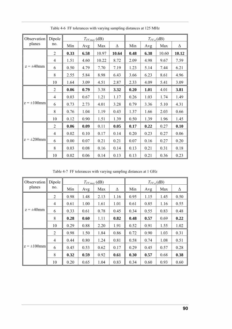
90

Table 4-6 FF tolerances with varying sampling distances at 125 MHz

TFF,max (dB) TFF,a (dB) Observation planes

Dipole no. Min Avg Max Δ Min Avg Max Δ

2 0.33 6.58 10.97 10.64 0.48 6.38 10.60 10.12 4 1.51 4.60 10.22 8.72 2.09 4.98 9.67 7.59

6 0.50 4.79 7.70 7.19 1.23 5.14 7.44 6.21

8 2.55 5.84 8.98 6.43 3.66 6.23 8.61 4.96

z = ±40mm

10 1.64 3.09 4.51 2.87 2.33 4.09 5.41 3.09

2 0.06 0.79 3.38 3.32 0.20 1.01 4.01 3.81

4 0.03 0.67 1.21 1.17 0.26 1.03 1.74 1.49

6 0.73 2.73 4.01 3.28 0.79 3.36 5.10 4.31

8 0.76 1.04 1.19 0.43 1.37 1.66 2.03 0.66

z = ±100mm

10 0.12 0.90 1.51 1.39 0.50 1.39 1.96 1.45

2 0.06 0.09 0.11 0.05 0.17 0.22 0.27 0.10

4 0.02 0.10 0.17 0.14 0.20 0.23 0.27 0.06

6 0.00 0.07 0.21 0.21 0.07 0.16 0.27 0.20

8 0.03 0.08 0.16 0.14 0.13 0.21 0.31 0.18

z = ±200mm

10 0.02 0.06 0.14 0.13 0.13 0.21 0.36 0.23

Table 4-7 FF tolerances with varying sampling distances at 1 GHz

TFF,max (dB) TFF,a (dB) Observation planes

Dipole no. Min Avg Max Δ Min Avg Max Δ

2 0.98 1.48 2.13 1.16 0.95 1.15 1.45 0.50 4 0.61 1.00 1.61 1.01 0.61 0.85 1.16 0.55

6 0.33 0.61 0.78 0.45 0.34 0.55 0.83 0.48

8 0.28 0.60 1.11 0.82 0.48 0.57 0.69 0.22

z = ±40mm

10 0.29 0.88 2.20 1.91 0.52 0.91 1.55 1.02

2 0.98 1.50 1.84 0.86 0.72 0.90 1.03 0.31

4 0.44 0.80 1.24 0.81 0.58 0.74 1.08 0.51

6 0.45 0.53 0.62 0.17 0.29 0.45 0.57 0.28

8 0.32 0.59 0.92 0.61 0.30 0.57 0.68 0.38

z = ±100mm

10 0.20 0.65 1.04 0.83 0.34 0.60 0.93 0.60

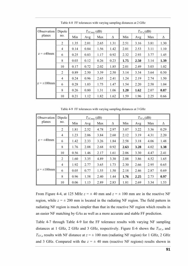
91

Table 4-8 FF tolerances with varying sampling distances at 2 GHz

TFF,max (dB) TFF,a (dB) Observation planes

Dipole no. Min Avg Max Δ Min Avg Max Δ

2 1.35 2.01 2.65 1.31 2.51 3.16 3.81 1.30 4 0.14 0.84 1.56 1.42 2.01 2.53 3.11 1.10

6 0.25 0.83 1.17 0.92 2.32 2.93 3.77 1.45

8 0.03 0.12 0.26 0.23 1.75 2.50 3.14 1.39

z = ±40mm

10 0.17 0.72 2.02 1.85 2.01 2.49 3.03 1.02

2 0.89 2.50 3.39 2.50 3.14 3.34 3.64 0.50

4 0.24 0.96 2.65 2.41 1.24 2.19 2.74 1.50

6 0.28 1.03 1.75 1.47 1.54 2.20 2.58 1.04

8 0.26 0.80 1.31 1.06 1.20 1.62 2.07 0.87

z = ±100mm

10 0.21 1.12 1.82 1.62 1.59 1.96 2.25 0.66

Table 4-9 FF tolerances with varying sampling distances at 3 GHz

TFF,max (dB) TFF,a (dB) Observation planes

Dipole no. Min Avg Max Δ Min Avg Max Δ

2 1.81 2.52 4.78 2.97 3.07 3.22 3.36 0.29 4 1.23 2.06 3.84 2.60 2.12 3.19 4.31 2.20

6 1.42 2.33 3.26 1.84 2.58 3.18 4.06 1.48

8 1.76 2.08 2.68 0.92 2.63 3.28 4.02 1.38

z = ±40mm

10 0.56 1.46 2.17 1.61 2.06 3.30 4.47 2.41

2 1.60 3.35 4.89 3.30 2.88 3.86 4.52 1.65

4 1.92 2.77 3.65 1.73 2.30 2.66 2.95 0.65

6 0.05 0.77 1.55 1.50 2.18 2.46 2.87 0.69

8 0.96 1.58 2.40 1.44 1.76 2.25 2.73 0.97

z = ±100mm

10 0.06 1.13 2.89 2.83 1.81 2.69 3.34 1.53

From Figure 4-4, at 125 MHz z = ± 40 mm and z = ± 100 mm are in the reactive NF

region, while z = ± 200 mm is located in the radiating NF region. The field pattern in

radiating NF region is much simpler than that in the reactive NF region which results in

an easier NF matching by GAs as well as a more accurate and stable FF prediction.

Table 4-7 through Table 4-9 list the FF tolerance results with varying NF sampling

distances at 1 GHz, 2 GHz and 3 GHz, respectively. Figure E-6 shows the TNF,a and

TFF,a results with NF distance at z = ± 100 mm (radiating NF region) for 1 GHz, 2 GHz

and 3 GHz. Compared with the z = ± 40 mm (reactive NF regions) results shown in

92

Figure E-2 through Figure E-4, with N =8 at 1 GHz both NF distances do not show an

obvious difference, while at 2 GHz and 3 GHz, NF distance at z = ± 100 mm results in a

better FF prediction than that at z = ± 40 mm.

Therefore NF data sampled from the radiating NF region are recommended for NF-FF

conversion, and will be applied later in this chapter.

4.5 Plane Coverage Angle

When using the planar sampling method, the plane coverage angle θ (see Figure 4-8)

should be considered. Assume a test PCB with an L × W rectangular shape is centred at

the x-y plane, the sampling plane has a rectangular square shape, each side of which is

l1, l2, l3 and l4 away from the z-axis, respectively, and the distance between these two

planes is h. Connect the corners of PCB plane and the sampling plane, respectively. The

angle between each line and the z-axis is recorded as θ1, θ2, θ3 and θ4, respectively.

2 21 2

1 1 2

2 21 2

2 2 3

2 21 2

3 3 4

2 21 2

4 4 1

cos / ;2 2

cos / ;2 2

cos / ;2 2

cos / .2 2

W Lh l l h

L Wh l l h

W Lh l l h

L Wh l l h

θ

θ

θ

θ

−

−

−

−

⎛ ⎞⎛ ⎞ ⎛ ⎞⎜ ⎟= − + − +⎜ ⎟ ⎜ ⎟⎜ ⎟⎝ ⎠ ⎝ ⎠⎝ ⎠⎛ ⎞⎛ ⎞ ⎛ ⎞⎜ ⎟= − + − +⎜ ⎟ ⎜ ⎟⎜ ⎟⎝ ⎠ ⎝ ⎠⎝ ⎠⎛ ⎞⎛ ⎞ ⎛ ⎞⎜ ⎟= − + − +⎜ ⎟ ⎜ ⎟⎜ ⎟⎝ ⎠ ⎝ ⎠⎝ ⎠⎛ ⎞⎛ ⎞ ⎛ ⎞⎜ ⎟= − + − +⎜ ⎟ ⎜ ⎟⎜ ⎟⎝ ⎠ ⎝ ⎠⎝ ⎠

(4-1)

The average of these four angles, θ, may be called ‘plane coverage angle’,

( )1 2 3 41 .4

θ θ θ θ θ= + + + (4-2)

The plane coverage angle is an important parameter for describing the coverage of a

closed surface around the PCB by an open sampling plane. As l1, l2, l3 and l4 increase

the plane coverage angle increases and approaches to 90˚ for l1, l2, l3 and l4 → ∞.

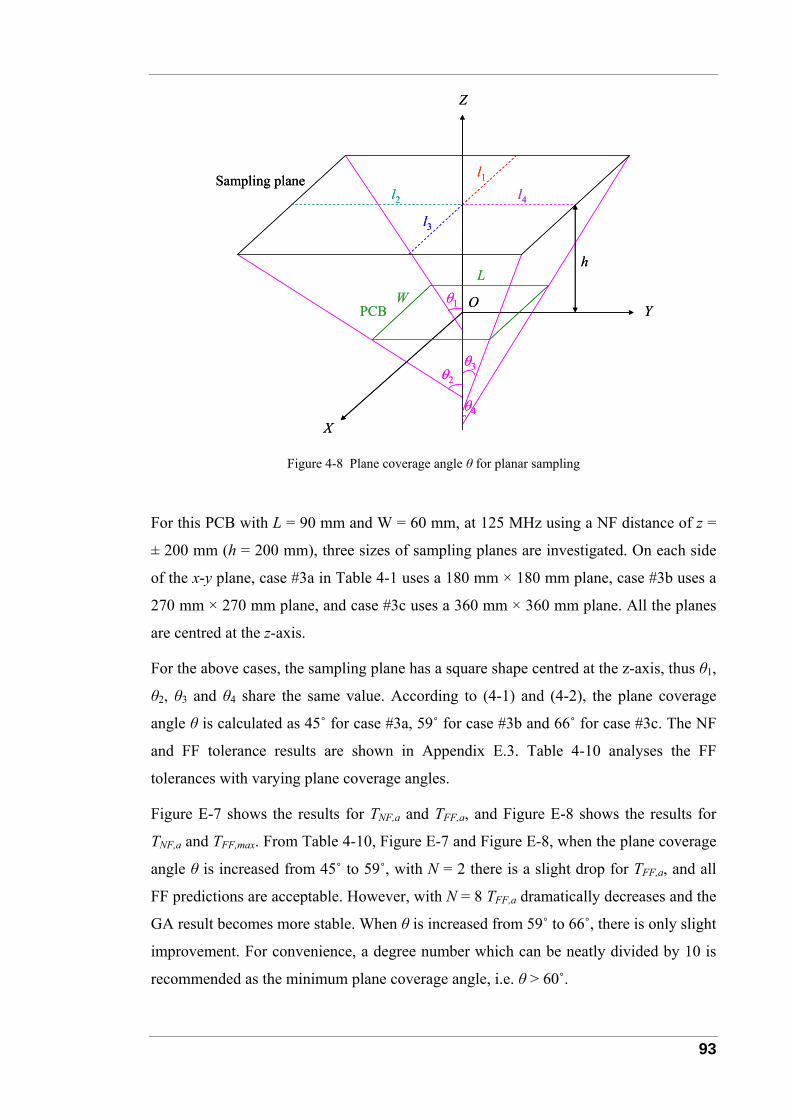
93

X

Z

Yθ1 OW

Lh

PCB

Sampling plane

θ3

θ4

θ2

l1

l2

l3

l4

X

Z

Yθ1 OW

Lh

PCB

Sampling plane

θ3

θ4

θ2

l1

l2

l3

l4

Figure 4-8 Plane coverage angle θ for planar sampling

For this PCB with L = 90 mm and W = 60 mm, at 125 MHz using a NF distance of z =

± 200 mm (h = 200 mm), three sizes of sampling planes are investigated. On each side

of the x-y plane, case #3a in Table 4-1 uses a 180 mm × 180 mm plane, case #3b uses a

270 mm × 270 mm plane, and case #3c uses a 360 mm × 360 mm plane. All the planes

are centred at the z-axis.

For the above cases, the sampling plane has a square shape centred at the z-axis, thus θ1,

θ2, θ3 and θ4 share the same value. According to (4-1) and (4-2), the plane coverage

angle θ is calculated as 45˚ for case #3a, 59˚ for case #3b and 66˚ for case #3c. The NF

and FF tolerance results are shown in Appendix E.3. Table 4-10 analyses the FF

tolerances with varying plane coverage angles.

Figure E-7 shows the results for TNF,a and TFF,a, and Figure E-8 shows the results for

TNF,a and TFF,max. From Table 4-10, Figure E-7 and Figure E-8, when the plane coverage

angle θ is increased from 45˚ to 59˚, with N = 2 there is a slight drop for TFF,a, and all

FF predictions are acceptable. However, with N = 8 TFF,a dramatically decreases and the

GA result becomes more stable. When θ is increased from 59˚ to 66˚, there is only slight

improvement. For convenience, a degree number which can be neatly divided by 10 is

recommended as the minimum plane coverage angle, i.e. θ > 60˚.

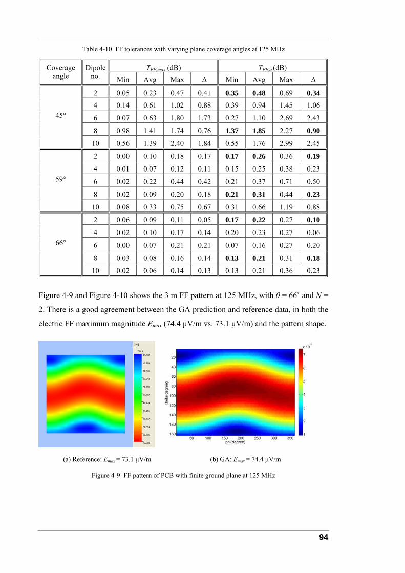
94

Table 4-10 FF tolerances with varying plane coverage angles at 125 MHz

TFF,max (dB) TFF,a (dB) Coverage angle

Dipole no. Min Avg Max Δ Min Avg Max Δ

2 0.05 0.23 0.47 0.41 0.35 0.48 0.69 0.34 4 0.14 0.61 1.02 0.88 0.39 0.94 1.45 1.06

6 0.07 0.63 1.80 1.73 0.27 1.10 2.69 2.43

8 0.98 1.41 1.74 0.76 1.37 1.85 2.27 0.90

45°

10 0.56 1.39 2.40 1.84 0.55 1.76 2.99 2.45

2 0.00 0.10 0.18 0.17 0.17 0.26 0.36 0.19

4 0.01 0.07 0.12 0.11 0.15 0.25 0.38 0.23

6 0.02 0.22 0.44 0.42 0.21 0.37 0.71 0.50

8 0.02 0.09 0.20 0.18 0.21 0.31 0.44 0.23

59°

10 0.08 0.33 0.75 0.67 0.31 0.66 1.19 0.88

2 0.06 0.09 0.11 0.05 0.17 0.22 0.27 0.10

4 0.02 0.10 0.17 0.14 0.20 0.23 0.27 0.06

6 0.00 0.07 0.21 0.21 0.07 0.16 0.27 0.20

8 0.03 0.08 0.16 0.14 0.13 0.21 0.31 0.18

66°

10 0.02 0.06 0.14 0.13 0.13 0.21 0.36 0.23

Figure 4-9 and Figure 4-10 shows the 3 m FF pattern at 125 MHz, with θ = 66˚ and N =

2. There is a good agreement between the GA prediction and reference data, in both the

electric FF maximum magnitude Emax (74.4 μV/m vs. 73.1 μV/m) and the pattern shape.

(a) Reference: Emax = 73.1 μV/m (b) GA: Emax = 74.4 μV/m

Figure 4-9 FF pattern of PCB with finite ground plane at 125 MHz

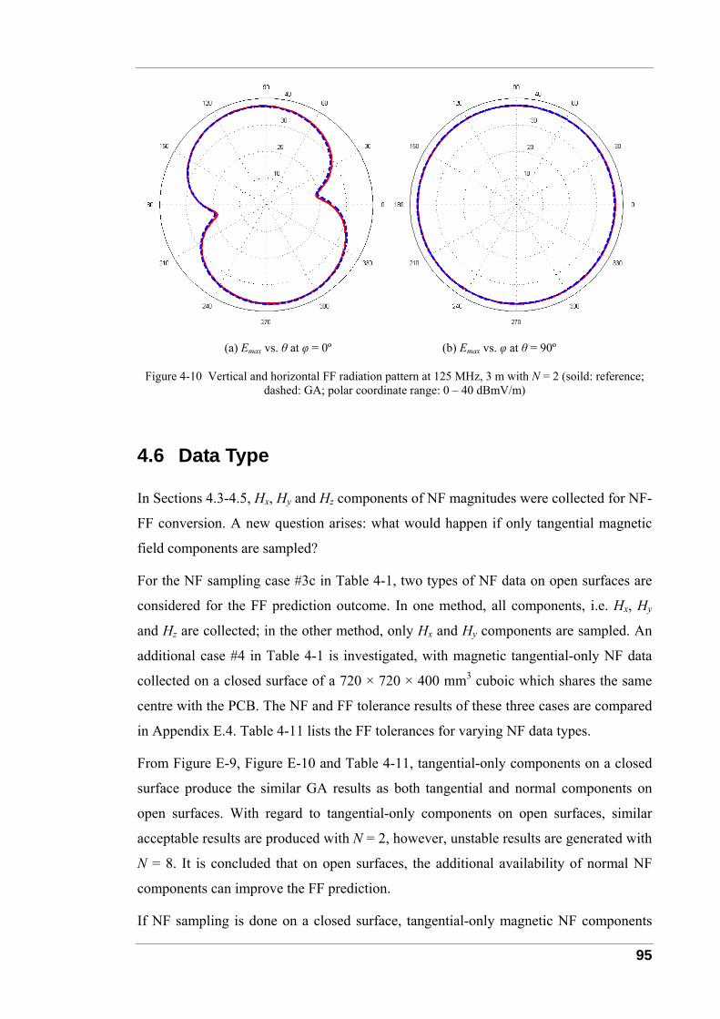
95

(a) Emax vs. θ at φ = 0º (b) Emax vs. φ at θ = 90º

Figure 4-10 Vertical and horizontal FF radiation pattern at 125 MHz, 3 m with N = 2 (soild: reference; dashed: GA; polar coordinate range: 0 – 40 dBmV/m)

4.6 Data Type

In Sections 4.3-4.5, Hx, Hy and Hz components of NF magnitudes were collected for NF-

FF conversion. A new question arises: what would happen if only tangential magnetic

field components are sampled?

For the NF sampling case #3c in Table 4-1, two types of NF data on open surfaces are

considered for the FF prediction outcome. In one method, all components, i.e. Hx, Hy

and Hz are collected; in the other method, only Hx and Hy components are sampled. An

additional case #4 in Table 4-1 is investigated, with magnetic tangential-only NF data

collected on a closed surface of a 720 × 720 × 400 mm3 cuboic which shares the same

centre with the PCB. The NF and FF tolerance results of these three cases are compared

in Appendix E.4. Table 4-11 lists the FF tolerances for varying NF data types.

From Figure E-9, Figure E-10 and Table 4-11, tangential-only components on a closed

surface produce the similar GA results as both tangential and normal components on

open surfaces. With regard to tangential-only components on open surfaces, similar

acceptable results are produced with N = 2, however, unstable results are generated with

N = 8. It is concluded that on open surfaces, the additional availability of normal NF

components can improve the FF prediction.

If NF sampling is done on a closed surface, tangential-only magnetic NF components

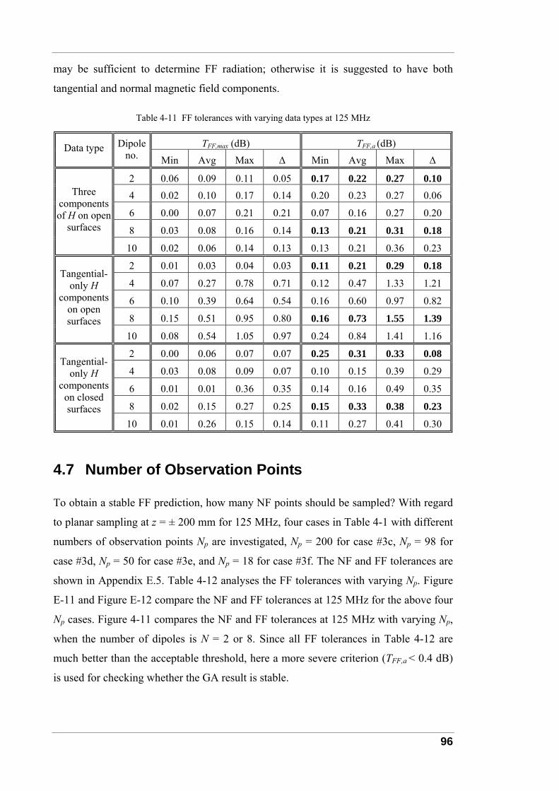
96

may be sufficient to determine FF radiation; otherwise it is suggested to have both

tangential and normal magnetic field components.

Table 4-11 FF tolerances with varying data types at 125 MHz

TFF,max (dB) TFF,a (dB) Data type Dipole no. Min Avg Max Δ Min Avg Max Δ

2 0.06 0.09 0.11 0.05 0.17 0.22 0.27 0.10 4 0.02 0.10 0.17 0.14 0.20 0.23 0.27 0.06

6 0.00 0.07 0.21 0.21 0.07 0.16 0.27 0.20

8 0.03 0.08 0.16 0.14 0.13 0.21 0.31 0.18

Three components of H on open

surfaces

10 0.02 0.06 0.14 0.13 0.13 0.21 0.36 0.23

2 0.01 0.03 0.04 0.03 0.11 0.21 0.29 0.18

4 0.07 0.27 0.78 0.71 0.12 0.47 1.33 1.21

6 0.10 0.39 0.64 0.54 0.16 0.60 0.97 0.82

8 0.15 0.51 0.95 0.80 0.16 0.73 1.55 1.39

Tangential-only H

components on open surfaces

10 0.08 0.54 1.05 0.97 0.24 0.84 1.41 1.16

2 0.00 0.06 0.07 0.07 0.25 0.31 0.33 0.08

4 0.03 0.08 0.09 0.07 0.10 0.15 0.39 0.29

6 0.01 0.01 0.36 0.35 0.14 0.16 0.49 0.35

8 0.02 0.15 0.27 0.25 0.15 0.33 0.38 0.23

Tangential-only H

components on closed surfaces

10 0.01 0.26 0.15 0.14 0.11 0.27 0.41 0.30

4.7 Number of Observation Points

To obtain a stable FF prediction, how many NF points should be sampled? With regard

to planar sampling at z = ± 200 mm for 125 MHz, four cases in Table 4-1 with different

numbers of observation points Np are investigated, Np = 200 for case #3c, Np = 98 for

case #3d, Np = 50 for case #3e, and Np = 18 for case #3f. The NF and FF tolerances are

shown in Appendix E.5. Table 4-12 analyses the FF tolerances with varying Np. Figure

E-11 and Figure E-12 compare the NF and FF tolerances at 125 MHz for the above four

Np cases. Figure 4-11 compares the NF and FF tolerances at 125 MHz with varying Np,

when the number of dipoles is N = 2 or 8. Since all FF tolerances in Table 4-12 are

much better than the acceptable threshold, here a more severe criterion (TFF,a < 0.4 dB)

is used for checking whether the GA result is stable.

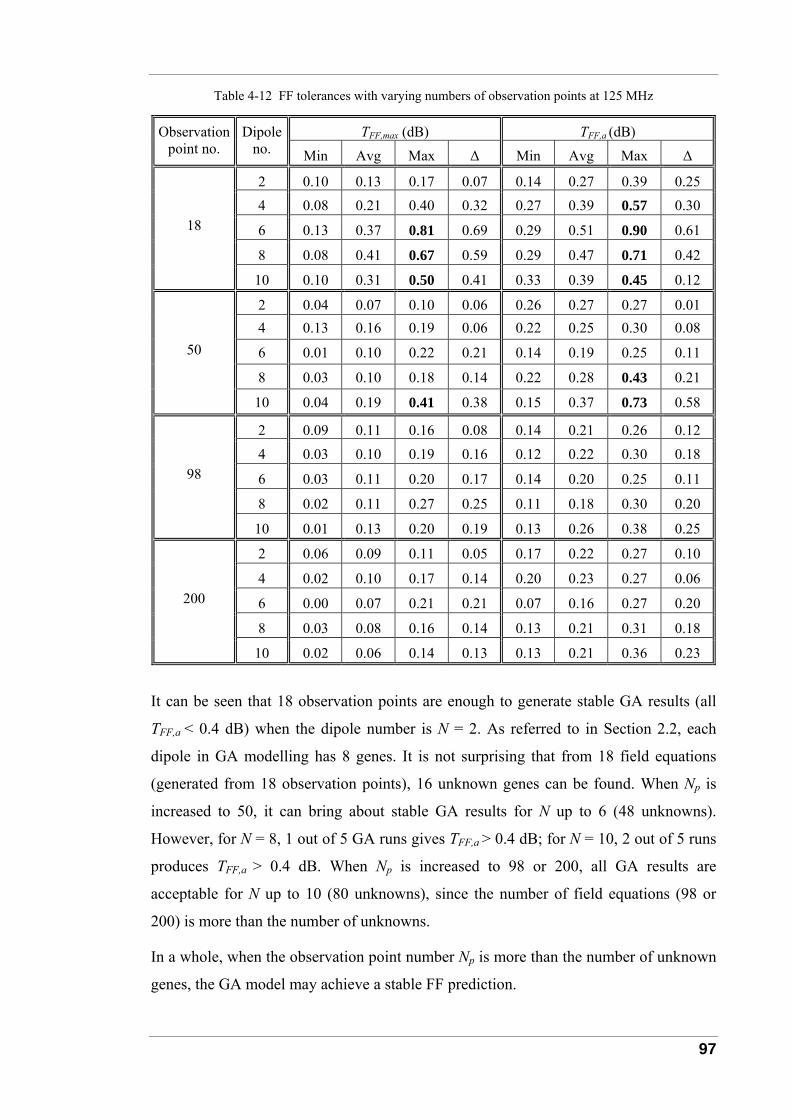
97

Table 4-12 FF tolerances with varying numbers of observation points at 125 MHz

TFF,max (dB) TFF,a (dB) Observation point no.

Dipole no. Min Avg Max Δ Min Avg Max Δ

2 0.10 0.13 0.17 0.07 0.14 0.27 0.39 0.25 4 0.08 0.21 0.40 0.32 0.27 0.39 0.57 0.30

6 0.13 0.37 0.81 0.69 0.29 0.51 0.90 0.61

8 0.08 0.41 0.67 0.59 0.29 0.47 0.71 0.42

18

10 0.10 0.31 0.50 0.41 0.33 0.39 0.45 0.12

2 0.04 0.07 0.10 0.06 0.26 0.27 0.27 0.01 4 0.13 0.16 0.19 0.06 0.22 0.25 0.30 0.08

6 0.01 0.10 0.22 0.21 0.14 0.19 0.25 0.11

8 0.03 0.10 0.18 0.14 0.22 0.28 0.43 0.21

50

10 0.04 0.19 0.41 0.38 0.15 0.37 0.73 0.58

2 0.09 0.11 0.16 0.08 0.14 0.21 0.26 0.12 4 0.03 0.10 0.19 0.16 0.12 0.22 0.30 0.18

6 0.03 0.11 0.20 0.17 0.14 0.20 0.25 0.11

8 0.02 0.11 0.27 0.25 0.11 0.18 0.30 0.20

98

10 0.01 0.13 0.20 0.19 0.13 0.26 0.38 0.25

2 0.06 0.09 0.11 0.05 0.17 0.22 0.27 0.10

4 0.02 0.10 0.17 0.14 0.20 0.23 0.27 0.06

6 0.00 0.07 0.21 0.21 0.07 0.16 0.27 0.20

8 0.03 0.08 0.16 0.14 0.13 0.21 0.31 0.18

200

10 0.02 0.06 0.14 0.13 0.13 0.21 0.36 0.23

It can be seen that 18 observation points are enough to generate stable GA results (all

TFF,a < 0.4 dB) when the dipole number is N = 2. As referred to in Section 2.2, each

dipole in GA modelling has 8 genes. It is not surprising that from 18 field equations

(generated from 18 observation points), 16 unknown genes can be found. When Np is

increased to 50, it can bring about stable GA results for N up to 6 (48 unknowns).

However, for N = 8, 1 out of 5 GA runs gives TFF,a > 0.4 dB; for N = 10, 2 out of 5 runs

produces TFF,a > 0.4 dB. When Np is increased to 98 or 200, all GA results are

acceptable for N up to 10 (80 unknowns), since the number of field equations (98 or

200) is more than the number of unknowns.

In a whole, when the observation point number Np is more than the number of unknown

genes, the GA model may achieve a stable FF prediction.

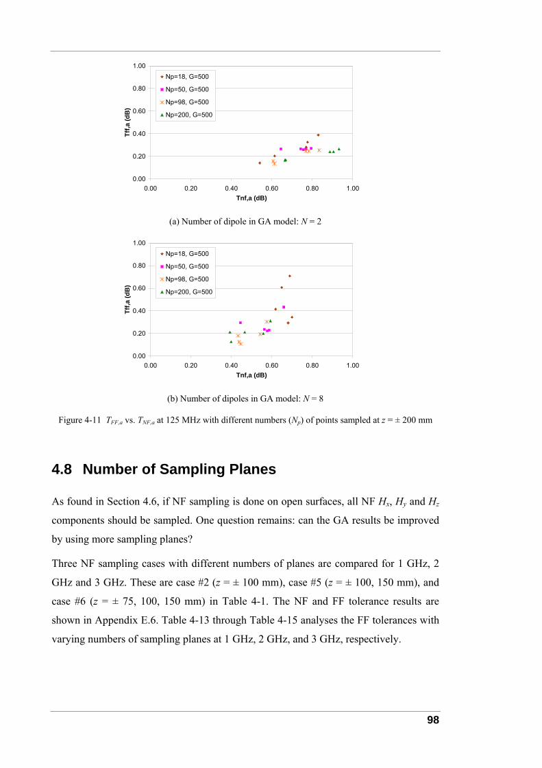
98

0.00

0.20

0.40

0.60

0.80

1.00

0.00 0.20 0.40 0.60 0.80 1.00Tnf,a (dB)

Tff,a

(dB

)

Np=18, G=500

Np=50, G=500

Np=98, G=500

Np=200, G=500

(a) Number of dipole in GA model: N = 2

0.00

0.20

0.40

0.60

0.80

1.00

0.00 0.20 0.40 0.60 0.80 1.00Tnf,a (dB)

Tff,a

(dB

)

Np=18, G=500

Np=50, G=500

Np=98, G=500

Np=200, G=500

(b) Number of dipoles in GA model: N = 8

Figure 4-11 TFF,a vs. TNF,a at 125 MHz with different numbers (Np) of points sampled at z = ± 200 mm

4.8 Number of Sampling Planes

As found in Section 4.6, if NF sampling is done on open surfaces, all NF Hx, Hy and Hz

components should be sampled. One question remains: can the GA results be improved

by using more sampling planes?

Three NF sampling cases with different numbers of planes are compared for 1 GHz, 2

GHz and 3 GHz. These are case #2 (z = ± 100 mm), case #5 (z = ± 100, 150 mm), and

case #6 (z = ± 75, 100, 150 mm) in Table 4-1. The NF and FF tolerance results are

shown in Appendix E.6. Table 4-13 through Table 4-15 analyses the FF tolerances with

varying numbers of sampling planes at 1 GHz, 2 GHz, and 3 GHz, respectively.

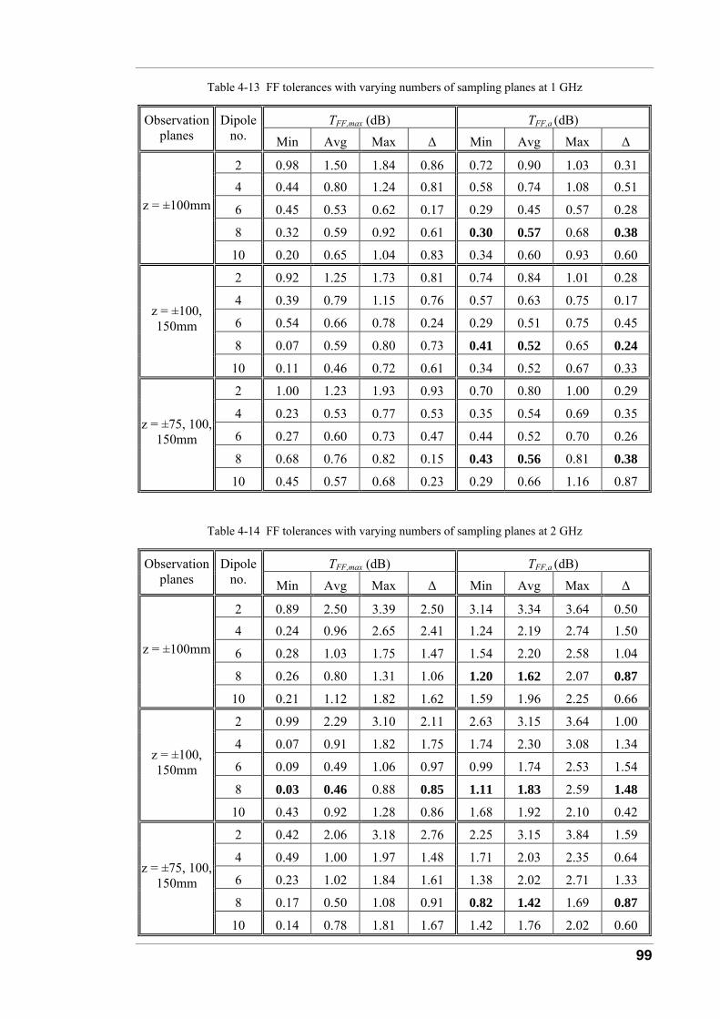
99

Table 4-13 FF tolerances with varying numbers of sampling planes at 1 GHz

TFF,max (dB) TFF,a (dB) Observation planes

Dipole no. Min Avg Max Δ Min Avg Max Δ

2 0.98 1.50 1.84 0.86 0.72 0.90 1.03 0.31 4 0.44 0.80 1.24 0.81 0.58 0.74 1.08 0.51

6 0.45 0.53 0.62 0.17 0.29 0.45 0.57 0.28

8 0.32 0.59 0.92 0.61 0.30 0.57 0.68 0.38

z = ±100mm

10 0.20 0.65 1.04 0.83 0.34 0.60 0.93 0.60

2 0.92 1.25 1.73 0.81 0.74 0.84 1.01 0.28

4 0.39 0.79 1.15 0.76 0.57 0.63 0.75 0.17

6 0.54 0.66 0.78 0.24 0.29 0.51 0.75 0.45

8 0.07 0.59 0.80 0.73 0.41 0.52 0.65 0.24

z = ±100, 150mm

10 0.11 0.46 0.72 0.61 0.34 0.52 0.67 0.33

2 1.00 1.23 1.93 0.93 0.70 0.80 1.00 0.29

4 0.23 0.53 0.77 0.53 0.35 0.54 0.69 0.35

6 0.27 0.60 0.73 0.47 0.44 0.52 0.70 0.26

8 0.68 0.76 0.82 0.15 0.43 0.56 0.81 0.38

z = ±75, 100, 150mm

10 0.45 0.57 0.68 0.23 0.29 0.66 1.16 0.87

Table 4-14 FF tolerances with varying numbers of sampling planes at 2 GHz

TFF,max (dB) TFF,a (dB) Observation planes

Dipole no. Min Avg Max Δ Min Avg Max Δ

2 0.89 2.50 3.39 2.50 3.14 3.34 3.64 0.50 4 0.24 0.96 2.65 2.41 1.24 2.19 2.74 1.50

6 0.28 1.03 1.75 1.47 1.54 2.20 2.58 1.04

8 0.26 0.80 1.31 1.06 1.20 1.62 2.07 0.87

z = ±100mm

10 0.21 1.12 1.82 1.62 1.59 1.96 2.25 0.66

2 0.99 2.29 3.10 2.11 2.63 3.15 3.64 1.00

4 0.07 0.91 1.82 1.75 1.74 2.30 3.08 1.34

6 0.09 0.49 1.06 0.97 0.99 1.74 2.53 1.54

8 0.03 0.46 0.88 0.85 1.11 1.83 2.59 1.48

z = ±100, 150mm

10 0.43 0.92 1.28 0.86 1.68 1.92 2.10 0.42

2 0.42 2.06 3.18 2.76 2.25 3.15 3.84 1.59

4 0.49 1.00 1.97 1.48 1.71 2.03 2.35 0.64

6 0.23 1.02 1.84 1.61 1.38 2.02 2.71 1.33

8 0.17 0.50 1.08 0.91 0.82 1.42 1.69 0.87

z = ±75, 100, 150mm

10 0.14 0.78 1.81 1.67 1.42 1.76 2.02 0.60

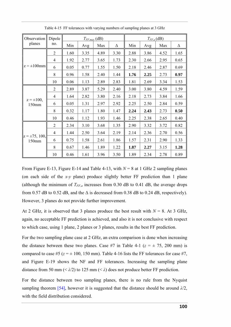
100

Table 4-15 FF tolerances with varying numbers of sampling planes at 3 GHz

TFF,max (dB) TFF,a (dB) Observation planes

Dipole no. Min Avg Max Δ Min Avg Max Δ

2 1.60 3.35 4.89 3.30 2.88 3.86 4.52 1.65 4 1.92 2.77 3.65 1.73 2.30 2.66 2.95 0.65

6 0.05 0.77 1.55 1.50 2.18 2.46 2.87 0.69

8 0.96 1.58 2.40 1.44 1.76 2.25 2.73 0.97

z = ±100mm

10 0.06 1.13 2.89 2.83 1.81 2.69 3.34 1.53

2 2.89 3.87 5.29 2.40 3.00 3.80 4.59 1.59

4 1.64 2.82 3.80 2.16 2.18 2.73 3.84 1.66

6 0.05 1.31 2.97 2.92 2.25 2.50 2.84 0.59

8 0.32 1.17 1.80 1.47 2.24 2.43 2.73 0.50

z = ±100, 150mm

10 0.46 1.12 1.93 1.46 2.25 2.38 2.65 0.40

2 2.34 3.10 3.68 1.35 2.90 3.32 3.72 0.82

4 1.44 2.50 3.64 2.19 2.14 2.36 2.70 0.56

6 0.75 1.58 2.61 1.86 1.57 2.31 2.90 1.33

8 0.67 1.46 1.89 1.22 1.87 2.27 3.15 1.28

z = ±75, 100, 150mm

10 0.46 1.61 3.96 3.50 1.89 2.34 2.78 0.89

From Figure E-13, Figure E-14 and Table 4-13, with N = 8 at 1 GHz 2 sampling planes

(on each side of the x-y plane) produce slightly better FF prediction than 1 plane

(although the minimum of TFF,a increases from 0.30 dB to 0.41 dB, the average drops

from 0.57 dB to 0.52 dB, and the Δ is decreased from 0.38 dB to 0.24 dB, respectively).

However, 3 planes do not provide further improvement.

At 2 GHz, it is observed that 3 planes produce the best result with N = 8. At 3 GHz,

again, no acceptable FF prediction is achieved, and also it is not conclusive with respect

to which case, using 1 plane, 2 planes or 3 planes, results in the best FF prediction.

For the two sampling plane case at 2 GHz, an extra comparison is done when increasing

the distance between these two planes. Case #7 in Table 4-1 (z = ± 75, 200 mm) is

compared to case #5 (z = ± 100, 150 mm). Table 4-16 lists the FF tolerances for case #7,

and Figure E-19 shows the NF and FF tolerances. Increasing the sampling plane

distance from 50 mm (< λ/2) to 125 mm (< λ) does not produce better FF prediction.

For the distance between two sampling planes, there is no rule from the Nyquist

sampling theorem [54], however it is suggested that the distance should be around λ/2,

with the field distribution considered.

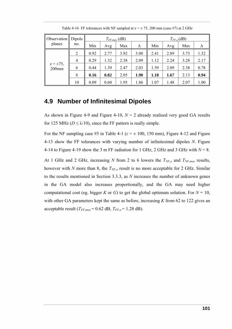
101

Table 4-16 FF tolerances with NF sampled at z = ± 75, 200 mm (case #7) at 2 GHz

TFF,max (dB) TFF,a (dB) Observation planes

Dipole no. Min Avg Max Δ Min Avg Max Δ

2 0.92 2.77 3.92 3.00 2.41 2.89 3.73 1.32 4 0.29 1.32 2.38 2.09 1.12 2.24 3.28 2.17

6 0.44 1.39 2.47 2.03 1.59 2.09 2.38 0.78

8 0.16 0.82 2.05 1.90 1.18 1.67 2.13 0.94

z = ±75, 200mm

10 0.09 0.60 1.95 1.86 1.07 1.48 2.07 1.00

4.9 Number of Infinitesimal Dipoles

As shown in Figure 4-9 and Figure 4-10, N = 2 already realised very good GA results

for 125 MHz (D ≤ λ/10), since the FF pattern is really simple.

For the NF sampling case #5 in Table 4-1 (z = ± 100, 150 mm), Figure 4-12 and Figure

4-13 show the FF tolerances with varying number of infinitesimal dipoles N. Figure

4-14 to Figure 4-19 show the 3 m FF radiation for 1 GHz, 2 GHz and 3 GHz with N = 8.

At 1 GHz and 2 GHz, increasing N from 2 to 6 lowers the TNF,a and TNF,max results,

however with N more than 8, the TNF,a result is no more acceptable for 2 GHz. Similar

to the results mentioned in Section 3.3.3, as N increases the number of unknown genes

in the GA model also increases proportionally, and the GA may need higher

computational cost (eg. bigger K or G) to get the global optimum solution. For N = 10,

with other GA parameters kept the same as before, increasing K from 62 to 122 gives an

acceptable result (TFF,max = 0.62 dB, TFF,a = 1.28 dB).

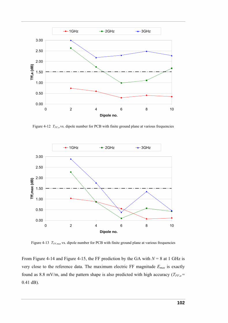
102

0.00

0.50

1.00

1.50

2.00

2.50

3.00

0 2 4 6 8 10

Dipole no.

Tff,a

(dB

)1GHz 2GHz 3GHz

Figure 4-12 TFF,a vs. dipole number for PCB with finite ground plane at various frequencies

0.00

0.50

1.00

1.50

2.00

2.50

3.00

0 2 4 6 8 10

Dipole no.

Tff,m

ax (d

B)

1GHz 2GHz 3GHz

Figure 4-13 TFF,max vs. dipole number for PCB with finite ground plane at various frequencies

From Figure 4-14 and Figure 4-15, the FF prediction by the GA with N = 8 at 1 GHz is

very close to the reference data. The maximum electric FF magnitude Emax is exactly

found as 8.8 mV/m, and the pattern shape is also predicted with high accuracy (TFF,a =

0.41 dB).

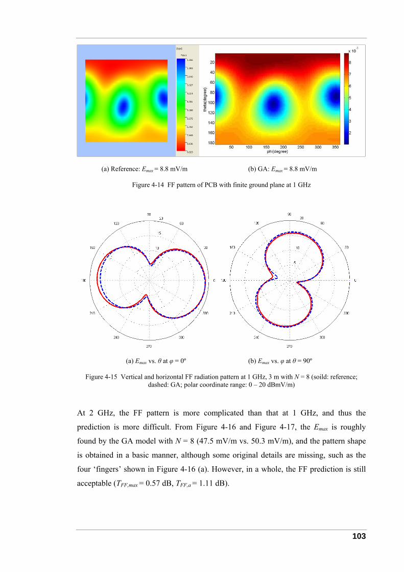
103

(a) Reference: Emax = 8.8 mV/m (b) GA: Emax = 8.8 mV/m

Figure 4-14 FF pattern of PCB with finite ground plane at 1 GHz

(a) Emax vs. θ at φ = 0º (b) Emax vs. φ at θ = 90º

Figure 4-15 Vertical and horizontal FF radiation pattern at 1 GHz, 3 m with N = 8 (soild: reference; dashed: GA; polar coordinate range: 0 – 20 dBmV/m)

At 2 GHz, the FF pattern is more complicated than that at 1 GHz, and thus the

prediction is more difficult. From Figure 4-16 and Figure 4-17, the Emax is roughly

found by the GA model with N = 8 (47.5 mV/m vs. 50.3 mV/m), and the pattern shape

is obtained in a basic manner, although some original details are missing, such as the

four ‘fingers’ shown in Figure 4-16 (a). However, in a whole, the FF prediction is still

acceptable (TFF,max = 0.57 dB, TFF,a = 1.11 dB).

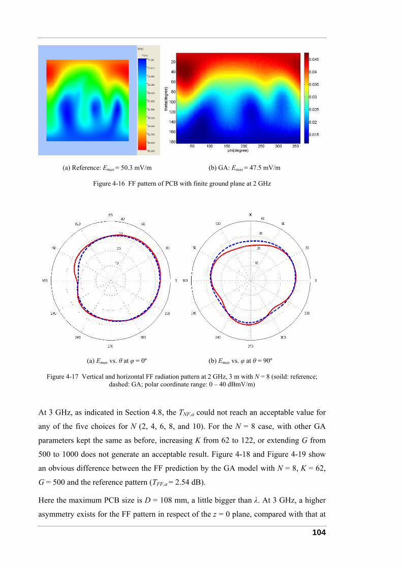
104

(a) Reference: Emax = 50.3 mV/m (b) GA: Emax = 47.5 mV/m

Figure 4-16 FF pattern of PCB with finite ground plane at 2 GHz

(a) Emax vs. θ at φ = 0º (b) Emax vs. φ at θ = 90º

Figure 4-17 Vertical and horizontal FF radiation pattern at 2 GHz, 3 m with N = 8 (soild: reference; dashed: GA; polar coordinate range: 0 – 40 dBmV/m)

At 3 GHz, as indicated in Section 4.8, the TNF,a could not reach an acceptable value for

any of the five choices for N (2, 4, 6, 8, and 10). For the N = 8 case, with other GA

parameters kept the same as before, increasing K from 62 to 122, or extending G from

500 to 1000 does not generate an acceptable result. Figure 4-18 and Figure 4-19 show

an obvious difference between the FF prediction by the GA model with N = 8, K = 62,

G = 500 and the reference pattern (TFF,a = 2.54 dB).

Here the maximum PCB size is D = 108 mm, a little bigger than λ. At 3 GHz, a higher

asymmetry exists for the FF pattern in respect of the z = 0 plane, compared with that at

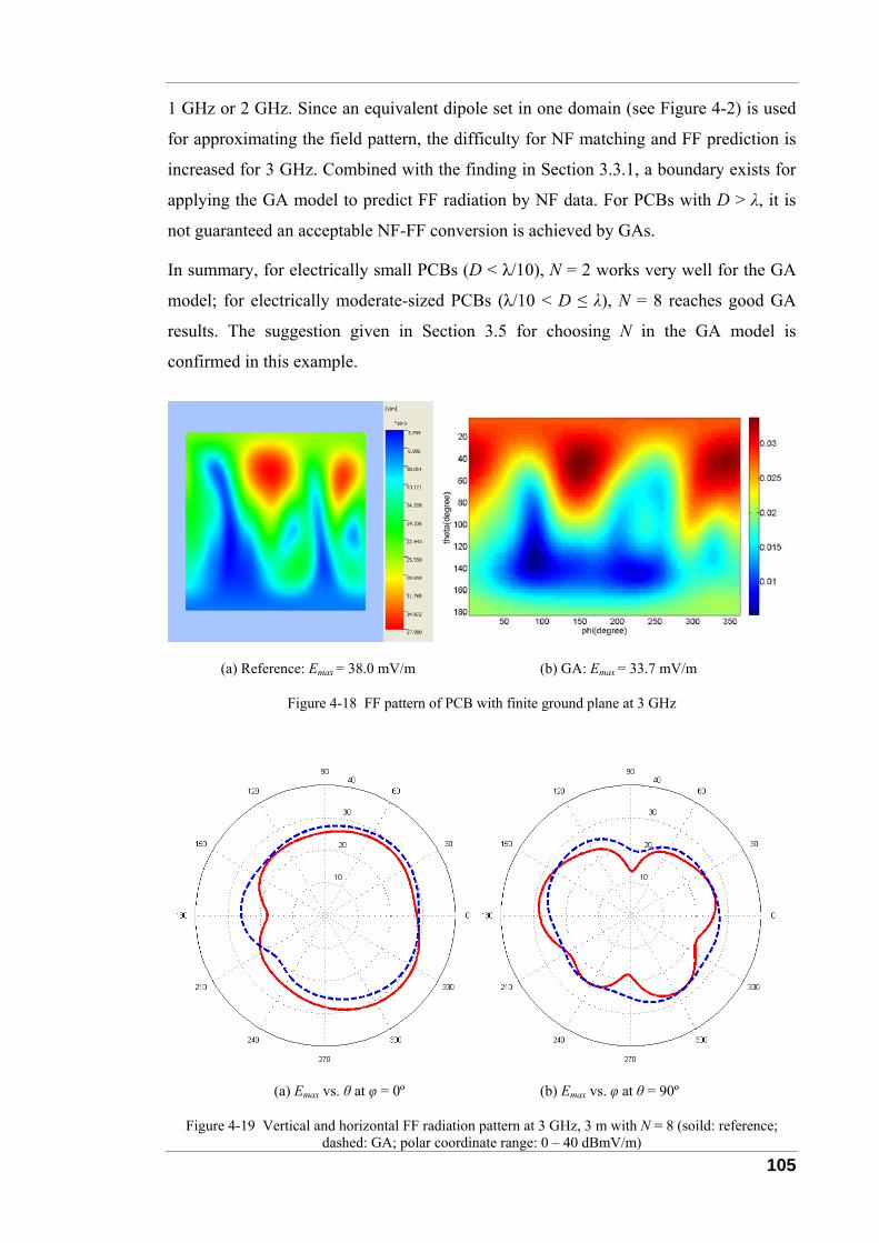
105

1 GHz or 2 GHz. Since an equivalent dipole set in one domain (see Figure 4-2) is used

for approximating the field pattern, the difficulty for NF matching and FF prediction is

increased for 3 GHz. Combined with the finding in Section 3.3.1, a boundary exists for

applying the GA model to predict FF radiation by NF data. For PCBs with D > λ, it is

not guaranteed an acceptable NF-FF conversion is achieved by GAs.

In summary, for electrically small PCBs (D < λ/10), N = 2 works very well for the GA

model; for electrically moderate-sized PCBs (λ/10 < D ≤ λ), N = 8 reaches good GA

results. The suggestion given in Section 3.5 for choosing N in the GA model is

confirmed in this example.

(a) Reference: Emax = 38.0 mV/m (b) GA: Emax = 33.7 mV/m

Figure 4-18 FF pattern of PCB with finite ground plane at 3 GHz

(a) Emax vs. θ at φ = 0º (b) Emax vs. φ at θ = 90º

Figure 4-19 Vertical and horizontal FF radiation pattern at 3 GHz, 3 m with N = 8 (soild: reference; dashed: GA; polar coordinate range: 0 – 40 dBmV/m)

106

4.10 Dynamic Data Range

Similar to Section 2.5.2.1, a dynamic data range is set for dealing with GA input data.

Among all M observation points, the maximum field value vmax and the minimum value

vmin are found. If vmin is more than adyn below vmax, the new minimum is set to vmax - adyn.

In Section 2.5.2.1, field values smaller than vmax - adyn were discarded, that is to say, the

points with these smallest field values were not involved in the GA process. Different

from the discarding method, here values smaller than vmax - adyn are replaced by vmax -

adyn. This new data process approach is closer to the dynamic range of measurement

equipment in practice by replacing small field strengths with the noise level of the

receiver.

With respect to NF sampling case #7 in Table 4-1 (z = ± 75, 200 mm) at 2 GHz, 20 GA

runs with the number of dipoles N = 8 are operated for five different dynamic data

ranges (adyn), 20 dB, 30 dB, 40 dB, 50 dB and 60 dB, respectively. Table 4-17 lists the

NF and FF tolerances and correlation results according to (2-30).

When the dynamic range adyn is too small, it is easy to realise a good NF matching (i.e. a

low TNF,a), but the correlation between TNF,a and TFF,a ( ), ,,NF a FF aCorr T T varies more;

when adyn is too big, ( ), ,,NF a FF aCorr T T is stable, but it is hard to obtain a low TNF,a.

From Table 4-17, based on the statistic data from 20 GA runs in each adyn case, the Avg

for TNF,a reaches the lowest value (1.91 dB) with adyn = 20 dB, while other cases have

roughly the same level of TNF,a (2.37 – 2.48 dB). However, the Δ for ( ), ,,NF a FF aCorr T T

with adyn = 20 or 30 dB is bigger than other cases (Δ = 0.13 – 0.24 vs. 0.07 – 0.10).

Also shown in Table 4-17 is a big variation for ( ), ,max,NF a FFCorr T T with 20 GA runs.

Among all five adyn cases, adyn = 40 dB obtains the most reliable FF prediction on the

maximum field magnitude (the Δ for ( ), ,max,NF a FFCorr T T is 0.34 vs. 0.60 – 0.80).

If an appropriate adyn is chosen, both ( ), ,max,NF a FFCorr T T and ( ), ,,NF a FF aCorr T T can

reach stable results. Taking into consideration the NF-FF tolerance correlation results, it

is recommended to set adyn as 40 dB for the NF-FF conversion in this example.

Figure 4-20 shows the NF observation points for case #7 in four sampling planes, each

of which contains a 10 × 10 sampling grid. The points #1 to #100 are located in the z =

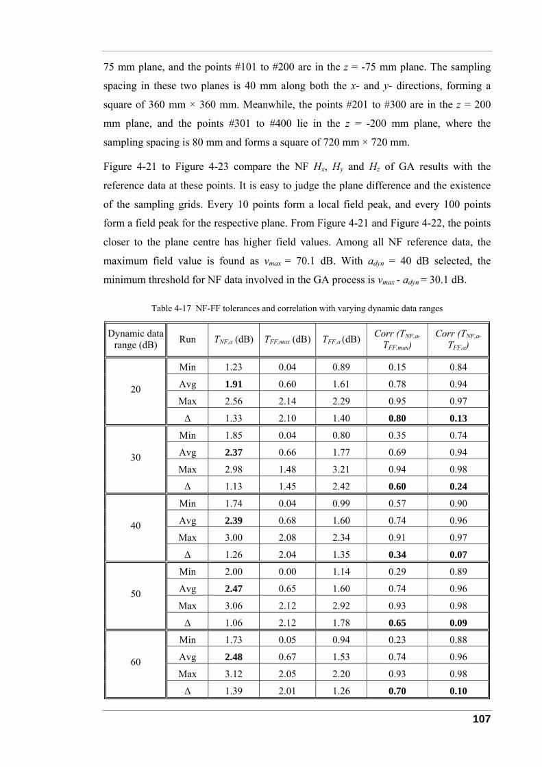
107

75 mm plane, and the points #101 to #200 are in the z = -75 mm plane. The sampling

spacing in these two planes is 40 mm along both the x- and y- directions, forming a

square of 360 mm × 360 mm. Meanwhile, the points #201 to #300 are in the z = 200

mm plane, and the points #301 to #400 lie in the z = -200 mm plane, where the

sampling spacing is 80 mm and forms a square of 720 mm × 720 mm.

Figure 4-21 to Figure 4-23 compare the NF Hx, Hy and Hz of GA results with the

reference data at these points. It is easy to judge the plane difference and the existence

of the sampling grids. Every 10 points form a local field peak, and every 100 points

form a field peak for the respective plane. From Figure 4-21 and Figure 4-22, the points

closer to the plane centre has higher field values. Among all NF reference data, the

maximum field value is found as vmax = 70.1 dB. With adyn = 40 dB selected, the

minimum threshold for NF data involved in the GA process is vmax - adyn = 30.1 dB.

Table 4-17 NF-FF tolerances and correlation with varying dynamic data ranges

Dynamic data range (dB) Run TNF,a (dB) TFF,max (dB) TFF,a (dB) Corr (TNF,a,

TFF,max) Corr (TNF,a,

TFF,a)

Min 1.23 0.04 0.89 0.15 0.84

Avg 1.91 0.60 1.61 0.78 0.94

Max 2.56 2.14 2.29 0.95 0.97 20

Δ 1.33 2.10 1.40 0.80 0.13

Min 1.85 0.04 0.80 0.35 0.74

Avg 2.37 0.66 1.77 0.69 0.94

Max 2.98 1.48 3.21 0.94 0.98 30

Δ 1.13 1.45 2.42 0.60 0.24

Min 1.74 0.04 0.99 0.57 0.90

Avg 2.39 0.68 1.60 0.74 0.96

Max 3.00 2.08 2.34 0.91 0.97 40

Δ 1.26 2.04 1.35 0.34 0.07

Min 2.00 0.00 1.14 0.29 0.89

Avg 2.47 0.65 1.60 0.74 0.96

Max 3.06 2.12 2.92 0.93 0.98 50

Δ 1.06 2.12 1.78 0.65 0.09

Min 1.73 0.05 0.94 0.23 0.88

Avg 2.48 0.67 1.53 0.74 0.96

Max 3.12 2.05 2.20 0.93 0.98 60

Δ 1.39 2.01 1.26 0.70 0.10

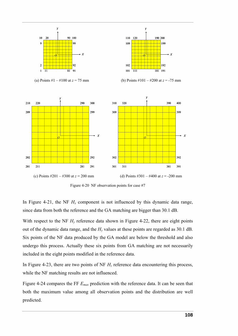
108

1 91

10 100

2

9

11

20

99

92

90

81

X

Y

O

1 91

10 100

2

9

11

20

99

92

90

81

X

Y

O

101 191

110 200

102

109

111

120

199

192

190

181

X

Y

O

101 191

110 200

102

109

111

120

199

192

190

181

X

Y

O

(a) Points #1 – #100 at z = 75 mm (b) Points #101 – #200 at z = -75 mm

201 291

210 300

202

209

211

220

299

292

290

281

X

Y

O

201 291

210 300

202

209

211

220

299

292

290

281

X

Y

O

301 391

310 400

302

309

311

320

399

392

390

381

X

Y

O

301 391

310 400

302

309

311

320

399

392

390

381

X

Y

O

(c) Points #201 – #300 at z = 200 mm (d) Points #301 – #400 at z = -200 mm

Figure 4-20 NF observation points for case #7

In Figure 4-21, the NF Hx component is not influenced by this dynamic data range,

since data from both the reference and the GA matching are bigger than 30.1 dB.

With respect to the NF Hy reference data shown in Figure 4-22, there are eight points

out of the dynamic data range, and the Hy values at these points are regarded as 30.1 dB.

Six points of the NF data produced by the GA model are below the threshold and also

undergo this process. Actually these six points from GA matching are not necessarily

included in the eight points modified in the reference data.

In Figure 4-23, there are two points of NF Hz reference data encountering this process,

while the NF matching results are not influenced.

Figure 4-24 compares the FF Emax prediction with the reference data. It can be seen that

both the maximum value among all observation points and the distribution are well

predicted.

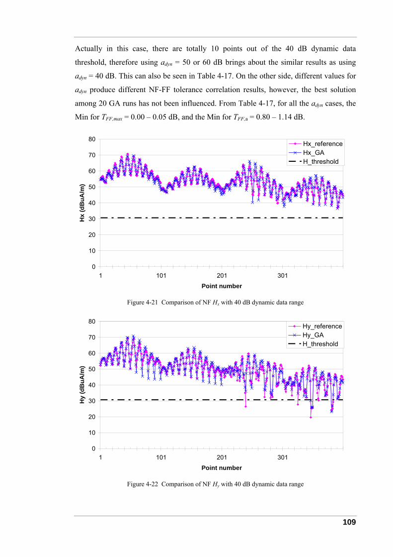
109

Actually in this case, there are totally 10 points out of the 40 dB dynamic data

threshold, therefore using adyn = 50 or 60 dB brings about the similar results as using

adyn = 40 dB. This can also be seen in Table 4-17. On the other side, different values for

adyn produce different NF-FF tolerance correlation results, however, the best solution

among 20 GA runs has not been influenced. From Table 4-17, for all the adyn cases, the

Min for TFF,max = 0.00 – 0.05 dB, and the Min for TFF,a = 0.80 – 1.14 dB.

0

10

20

30

40

50

60

70

80

1 101 201 301

Point number

Hx

(dB

uA/m

)

Hx_referenceHx_GAH_threshold

Figure 4-21 Comparison of NF Hx with 40 dB dynamic data range

0

10

20

30

40

50

60

70

80

1 101 201 301

Point number

Hy

(dB

uA/m

)

Hy_referenceHy_GAH_threshold

Figure 4-22 Comparison of NF Hy with 40 dB dynamic data range

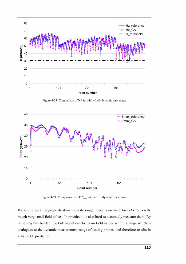
110

0

10

20

30

40

50

60

70

80

1 101 201 301

Point number

Hz

(dB

uA/m

)Hz_referenceHz_GAH_threshold

Figure 4-23 Comparison of NF Hz with 40 dB dynamic data range

10

15

20

25

30

35

40

1 51 101 151Point number

Emax

(dB

mV/

m)

Emax_referenceEmax_GA

Figure 4-24 Comparison of FF Emax with 40 dB dynamic data range

By setting up an appropriate dynamic data range, there is no need for GAs to exactly

match very small field values. In practice it is also hard to accurately measure them. By

removing this burden, the GA model can focus on field values within a range which is

analogues to the dynamic measurement range of testing probes, and therefore results in

a stable FF prediction.

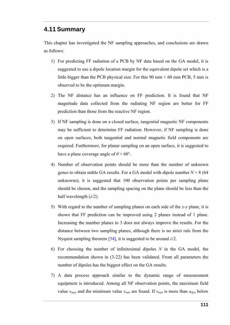
111

4.11 Summary

This chapter has investigated the NF sampling approaches, and conclusions are drawn

as follows:

1) For predicting FF radiation of a PCB by NF data based on the GA model, it is

suggested to use a dipole location margin for the equivalent dipole set which is a

little bigger than the PCB physical size. For this 90 mm × 60 mm PCB, 5 mm is

observed to be the optimum margin.

2) The NF distance has an influence on FF prediction. It is found that NF

magnitude data collected from the radiating NF region are better for FF

prediction than those from the reactive NF region.

3) If NF sampling is done on a closed surface, tangential magnetic NF components

may be sufficient to determine FF radiation. However, if NF sampling is done

on open surfaces, both tangential and normal magnetic field components are

required. Furthermore, for planar sampling on an open surface, it is suggested to

have a plane coverage angle of θ > 60°.

4) Number of observation points should be more than the number of unknown

genes to obtain stable GA results. For a GA model with dipole number N = 8 (64

unknowns), it is suggested that 100 observation points per sampling plane

should be chosen, and the sampling spacing on the plane should be less than the

half wavelength (λ/2).

5) With regard to the number of sampling planes on each side of the x-y plane, it is

shown that FF prediction can be improved using 2 planes instead of 1 plane.

Increasing the number planes to 3 does not always improve the results. For the

distance between two sampling planes, although there is no strict rule from the

Nyquist sampling theorem [54], it is suggested to be around λ/2.

6) For choosing the number of infinitesimal dipoles N in the GA model, the

recommendation shown in (3-22) has been validated. From all parameters the

number of dipoles has the biggest effect on the GA results.

7) A data process approach similar to the dynamic range of measurement

equipment is introduced. Among all NF observation points, the maximum field

value vmax and the minimum value vmin are found. If vmin is more than adyn below

112

vmax, the new minimum is set to vmax - adyn. Field values smaller than vmax - adyn

are replaced by vmax - adyn, and kept in the GA process. Taking into account the

NF-FF tolerance correlation, in this example 40 dB is recommended for the NF-

FF conversion.

113

5 Near Field-Far Field Conversion Case Studies

This chapter presents two case studies about NF-FF conversion, where the findings in

Chapter 4 are applied to engineering practice.

Outline

This chapter includes two sections, Section 5.1 investigates the radiation of a PCB with

a microstrip trace on an infinite ground plane, where the image theory [2][4][52] is

applied to the GA modelling, and NF data sampled from the reactive NF region and the

radiating NF region are compared for the FF prediction outcome. Section 5.2 uses

magnetic NF magnitude measurements to predict the FF radiation of an electrically

large loop in free space.

Contributions

The main contributions of this chapter are the confirmation of the findings in Chapter 4:

1) Compared with the reactive NF region, the radiating NF region is better for

converting the NF data to FF radiation. This is validated by simulated NF data

from a microstrip trace above an infinite ground plane, and also by NF

measurements from an electrically large loop in free space.

2) Magnetic NF magnitudes (Hx, Hy and Hz) on two planes are sufficient for NF-

FF conversion, if the plane coverage angle is big enough and also there are

enough sampling points. If tangential-only NF components are measured, NF

data along the lateral sides of PCBs are also needed for NF-FF conversion.

5.1 Microstrip Trace

Section 3 investigated the FF behaviour of a long wire, a large loop and a power ground

plane pair. All of them were placed in free space. Section 4 discussed the NF-FF

conversion for a PCB with a finite ground plane. This section applies the GA to a

different application, predicting FF radiation by NF data for a PCB above an infinite

ground plane. Using the image theory [2][4][52], an equivalent dipole set and its image

in respect of the ground plane together reconstruct the FF pattern.

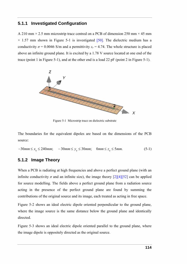
114

5.1.1 Investigated Configuration

A 210 mm × 2.5 mm microstrip trace centred on a PCB of dimension 250 mm × 45 mm

× 1.57 mm shown in Figure 5-1 is investigated [50]. The dielectric medium has a

conductivity σ = 0.0046 S/m and a permittivity εr = 4.74. The whole structure is placed

above an infinite ground plane. It is excited by a 1.78 V source located at one end of the

trace (point 1 in Figure 5-1), and at the other end is a load 22 pF (point 2 in Figure 5-1).

Figure 5-1 Microstrip trace on dielectric substrate

The boundaries for the equivalent dipoles are based on the dimensions of the PCB

source:

30 240 ; 30 30 ; 0 5 .q q qmm x mm mm y mm mm z mm− ≤ ≤ − ≤ ≤ ≤ ≤ (5-1)

5.1.2 Image Theory

When a PCB is radiating at high frequencies and above a perfect ground plane (with an

infinite conductivity σ and an infinite size), the image theory [2][4][52] can be applied

for source modelling. The fields above a perfect ground plane from a radiation source

acting in the presence of the perfect ground plane are found by summing the

contributions of the original source and its image, each treated as acting in free space.

Figure 5-2 shows an ideal electric dipole oriented perpendicular to the ground plane,

where the image source is the same distance below the ground plane and identically

directed.

Figure 5-3 shows an ideal electric dipole oriented parallel to the ground plane, where

the image dipole is oppositely directed as the original source.

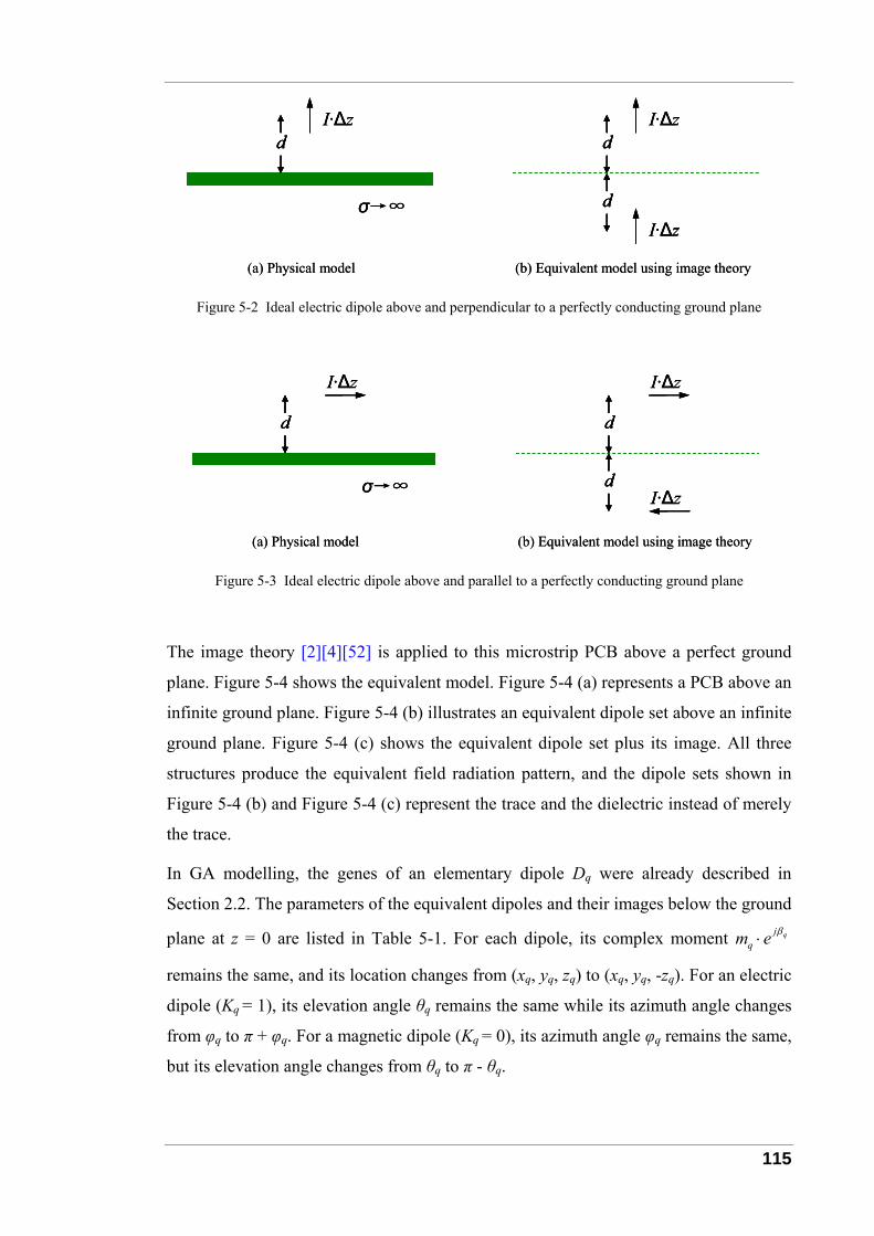
115

(a) Physical model (b) Equivalent model using image theory

dI·Δz

dI·Δz

dI·Δz

σ→∞

(a) Physical model (b) Equivalent model using image theory

dI·Δz

dI·Δz

dI·Δz

σ→∞

ddI·Δz

ddI·Δz

ddI·Δz

σ→∞

Figure 5-2 Ideal electric dipole above and perpendicular to a perfectly conducting ground plane

d

I·Δz

σ→∞

d

d

I·Δz

I·Δz

(a) Physical model (b) Equivalent model using image theory

d

I·Δz

σ→∞

d

d

I·Δz

I·Δz

dd

I·Δz

σ→∞

dd

dd

I·Δz

I·Δz

(a) Physical model (b) Equivalent model using image theory

Figure 5-3 Ideal electric dipole above and parallel to a perfectly conducting ground plane

The image theory [2][4][52] is applied to this microstrip PCB above a perfect ground

plane. Figure 5-4 shows the equivalent model. Figure 5-4 (a) represents a PCB above an

infinite ground plane. Figure 5-4 (b) illustrates an equivalent dipole set above an infinite

ground plane. Figure 5-4 (c) shows the equivalent dipole set plus its image. All three

structures produce the equivalent field radiation pattern, and the dipole sets shown in

Figure 5-4 (b) and Figure 5-4 (c) represent the trace and the dielectric instead of merely

the trace.

In GA modelling, the genes of an elementary dipole Dq were already described in

Section 2.2. The parameters of the equivalent dipoles and their images below the ground

plane at z = 0 are listed in Table 5-1. For each dipole, its complex moment qjqm e β⋅

remains the same, and its location changes from (xq, yq, zq) to (xq, yq, -zq). For an electric

dipole (Kq = 1), its elevation angle θq remains the same while its azimuth angle changes

from φq to π + φq. For a magnetic dipole (Kq = 0), its azimuth angle φq remains the same,

but its elevation angle changes from θq to π - θq.

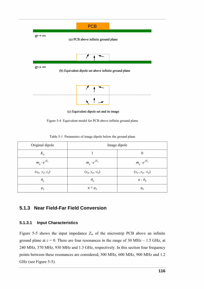
116

(a) PCB above infinite ground planeσ→∞

PCB

(a) PCB above infinite ground planeσ→∞

PCB

(b) Equivalent dipole set above infinite ground planeσ→∞

(b) Equivalent dipole set above infinite ground planeσ→∞

(c) Equivalent dipole set and its image(c) Equivalent dipole set and its image

Figure 5-4 Equivalent model for PCB above infinite ground plane

Table 5-1 Parameters of image dipole below the ground plane

Original dipole Image dipole

Kq 1 0

qjqm e β⋅ qj

qm e β⋅ qjqm e β⋅

(xq, yq, zq) (xq, yq, -zq) (xq , yq, -zq)

θq θq π - θq

φq π + φq φq

5.1.3 Near Field-Far Field Conversion

5.1.3.1 Input Characteristics

Figure 5-5 shows the input impedance Zin of the microstrip PCB above an infinite

ground plane at z = 0. There are four resonances in the range of 30 MHz – 1.5 GHz, at

240 MHz, 570 MHz, 930 MHz and 1.3 GHz, respectively. In this section four frequency

points between these resonances are considered, 300 MHz, 600 MHz, 900 MHz and 1.2

GHz (see Figure 5-5).

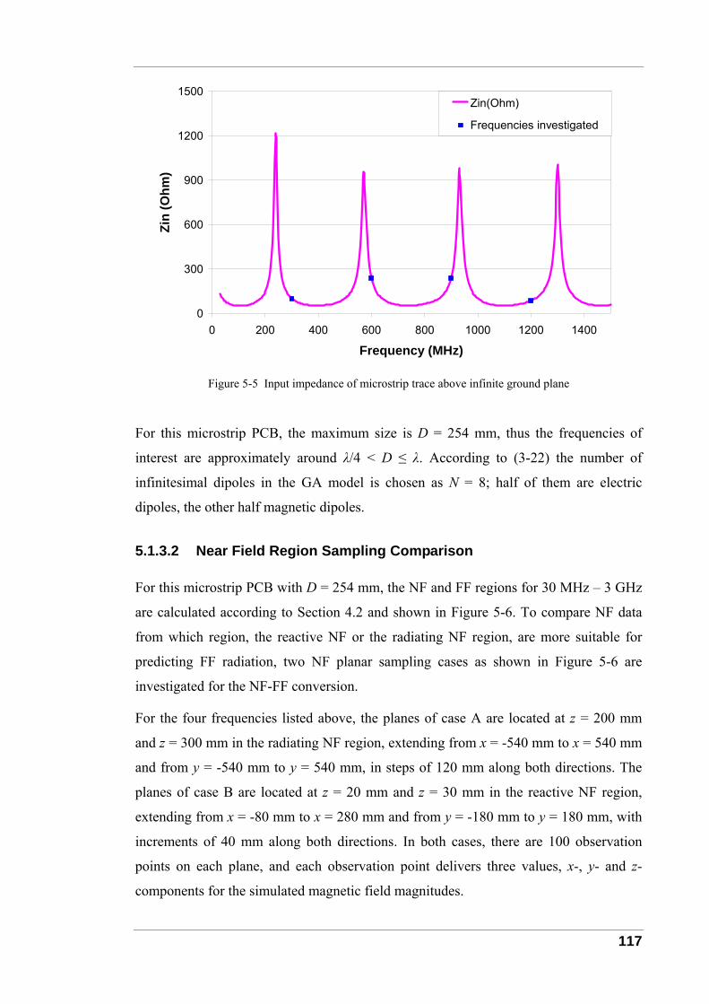
117

0

300

600

900

1200

1500

0 200 400 600 800 1000 1200 1400

Frequency (MHz)

Zin

(Ohm

)

Zin(Ohm)

Frequencies investigated

Figure 5-5 Input impedance of microstrip trace above infinite ground plane

For this microstrip PCB, the maximum size is D = 254 mm, thus the frequencies of

interest are approximately around λ/4 < D ≤ λ. According to (3-22) the number of

infinitesimal dipoles in the GA model is chosen as N = 8; half of them are electric

dipoles, the other half magnetic dipoles.

5.1.3.2 Near Field Region Sampling Comparison

For this microstrip PCB with D = 254 mm, the NF and FF regions for 30 MHz – 3 GHz

are calculated according to Section 4.2 and shown in Figure 5-6. To compare NF data

from which region, the reactive NF or the radiating NF region, are more suitable for

predicting FF radiation, two NF planar sampling cases as shown in Figure 5-6 are

investigated for the NF-FF conversion.

For the four frequencies listed above, the planes of case A are located at z = 200 mm

and z = 300 mm in the radiating NF region, extending from x = -540 mm to x = 540 mm

and from y = -540 mm to y = 540 mm, in steps of 120 mm along both directions. The

planes of case B are located at z = 20 mm and z = 30 mm in the reactive NF region,

extending from x = -80 mm to x = 280 mm and from y = -180 mm to y = 180 mm, with

increments of 40 mm along both directions. In both cases, there are 100 observation

points on each plane, and each observation point delivers three values, x-, y- and z-

components for the simulated magnetic field magnitudes.

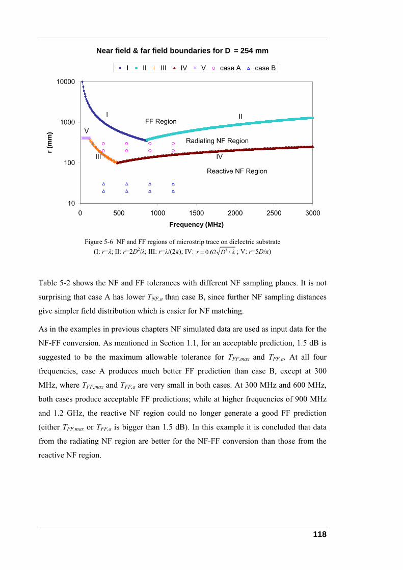
118

Near field & far field boundaries for D = 254 mm

10

100

1000

10000

0 500 1000 1500 2000 2500 3000

Frequency (MHz)

r (m

m)

I II III IV V case A case B

FF Region

Radiating NF Region

Reactive NF Region

I II

V

IVIII

Figure 5-6 NF and FF regions of microstrip trace on dielectric substrate (I: r=λ; II: r=2D2/λ; III: r=λ/(2π); IV: 30.62 /r D λ= ; V: r=5D/π)

Table 5-2 shows the NF and FF tolerances with different NF sampling planes. It is not

surprising that case A has lower TNF,a than case B, since further NF sampling distances

give simpler field distribution which is easier for NF matching.

As in the examples in previous chapters NF simulated data are used as input data for the

NF-FF conversion. As mentioned in Section 1.1, for an acceptable prediction, 1.5 dB is

suggested to be the maximum allowable tolerance for TFF,max and TFF,a. At all four

frequencies, case A produces much better FF prediction than case B, except at 300

MHz, where TFF,max and TFF,a are very small in both cases. At 300 MHz and 600 MHz,

both cases produce acceptable FF predictions; while at higher frequencies of 900 MHz

and 1.2 GHz, the reactive NF region could no longer generate a good FF prediction

(either TFF,max or TFF,a is bigger than 1.5 dB). In this example it is concluded that data

from the radiating NF region are better for the NF-FF conversion than those from the

reactive NF region.

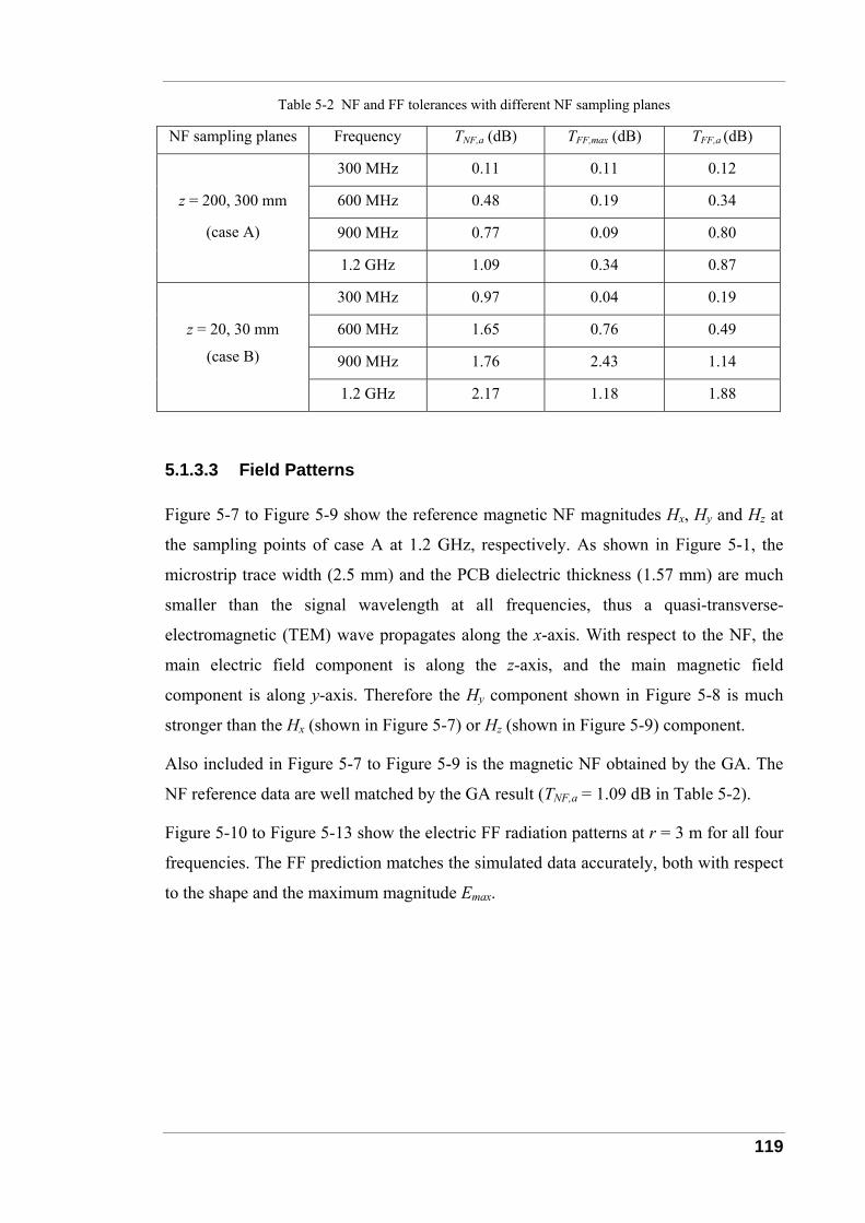
119

Table 5-2 NF and FF tolerances with different NF sampling planes

NF sampling planes Frequency TNF,a (dB) TFF,max (dB) TFF,a (dB)

300 MHz 0.11 0.11 0.12

600 MHz 0.48 0.19 0.34

900 MHz 0.77 0.09 0.80

z = 200, 300 mm

(case A)

1.2 GHz 1.09 0.34 0.87

300 MHz 0.97 0.04 0.19

600 MHz 1.65 0.76 0.49

900 MHz 1.76 2.43 1.14

z = 20, 30 mm

(case B)

1.2 GHz 2.17 1.18 1.88

5.1.3.3 Field Patterns

Figure 5-7 to Figure 5-9 show the reference magnetic NF magnitudes Hx, Hy and Hz at

the sampling points of case A at 1.2 GHz, respectively. As shown in Figure 5-1, the

microstrip trace width (2.5 mm) and the PCB dielectric thickness (1.57 mm) are much

smaller than the signal wavelength at all frequencies, thus a quasi-transverse-

electromagnetic (TEM) wave propagates along the x-axis. With respect to the NF, the

main electric field component is along the z-axis, and the main magnetic field

component is along y-axis. Therefore the Hy component shown in Figure 5-8 is much

stronger than the Hx (shown in Figure 5-7) or Hz (shown in Figure 5-9) component.

Also included in Figure 5-7 to Figure 5-9 is the magnetic NF obtained by the GA. The

NF reference data are well matched by the GA result (TNF,a = 1.09 dB in Table 5-2).

Figure 5-10 to Figure 5-13 show the electric FF radiation patterns at r = 3 m for all four

frequencies. The FF prediction matches the simulated data accurately, both with respect

to the shape and the maximum magnitude Emax.

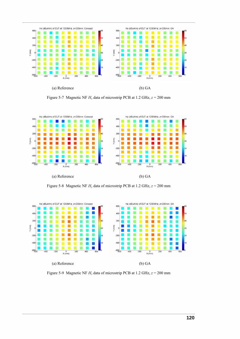
120

(a) Reference (b) GA

Figure 5-7 Magnetic NF Hx data of microstrip PCB at 1.2 GHz, z = 200 mm

(a) Reference (b) GA

Figure 5-8 Magnetic NF Hy data of microstrip PCB at 1.2 GHz, z = 200 mm

(a) Reference (b) GA

Figure 5-9 Magnetic NF Hz data of microstrip PCB at 1.2 GHz, z = 200 mm

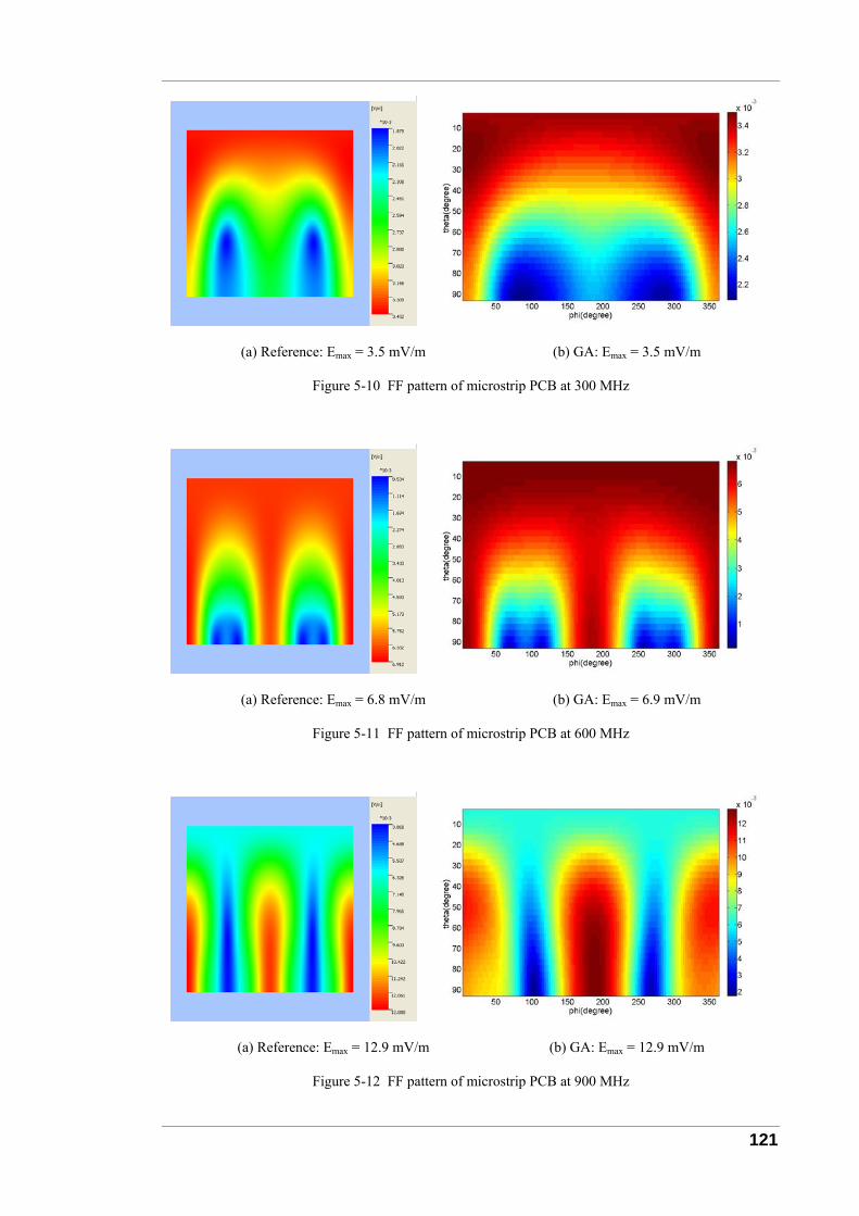
121

(a) Reference: Emax = 3.5 mV/m (b) GA: Emax = 3.5 mV/m

Figure 5-10 FF pattern of microstrip PCB at 300 MHz

(a) Reference: Emax = 6.8 mV/m (b) GA: Emax = 6.9 mV/m

Figure 5-11 FF pattern of microstrip PCB at 600 MHz

(a) Reference: Emax = 12.9 mV/m (b) GA: Emax = 12.9 mV/m

Figure 5-12 FF pattern of microstrip PCB at 900 MHz

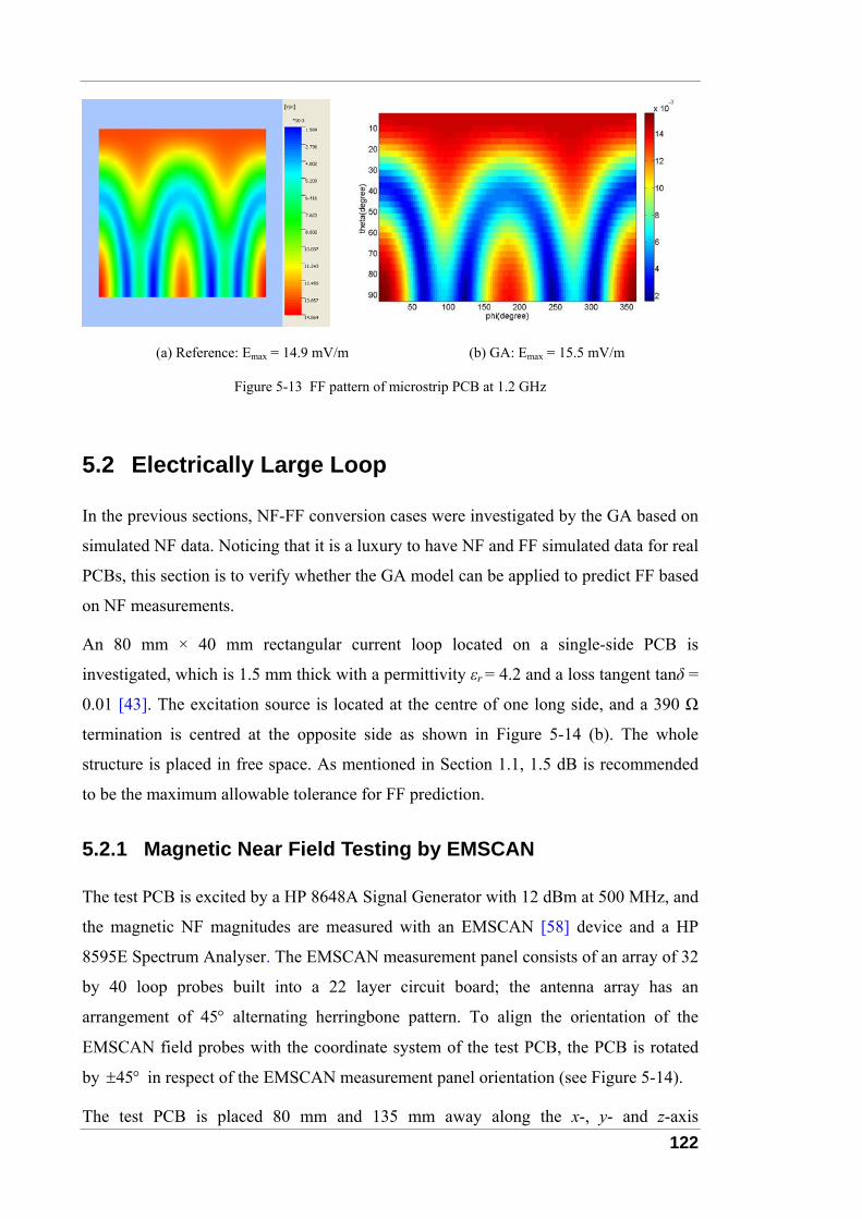
122

(a) Reference: Emax = 14.9 mV/m (b) GA: Emax = 15.5 mV/m

Figure 5-13 FF pattern of microstrip PCB at 1.2 GHz

5.2 Electrically Large Loop

In the previous sections, NF-FF conversion cases were investigated by the GA based on

simulated NF data. Noticing that it is a luxury to have NF and FF simulated data for real

PCBs, this section is to verify whether the GA model can be applied to predict FF based

on NF measurements.

An 80 mm × 40 mm rectangular current loop located on a single-side PCB is

investigated, which is 1.5 mm thick with a permittivity εr = 4.2 and a loss tangent tanδ =

0.01 [43]. The excitation source is located at the centre of one long side, and a 390 Ω

termination is centred at the opposite side as shown in Figure 5-14 (b). The whole

structure is placed in free space. As mentioned in Section 1.1, 1.5 dB is recommended

to be the maximum allowable tolerance for FF prediction.

5.2.1 Magnetic Near Field Testing by EMSCAN

The test PCB is excited by a HP 8648A Signal Generator with 12 dBm at 500 MHz, and

the magnetic NF magnitudes are measured with an EMSCAN [58] device and a HP

8595E Spectrum Analyser. The EMSCAN measurement panel consists of an array of 32

by 40 loop probes built into a 22 layer circuit board; the antenna array has an

arrangement of 45° alternating herringbone pattern. To align the orientation of the

EMSCAN field probes with the coordinate system of the test PCB, the PCB is rotated

by 45± ° in respect of the EMSCAN measurement panel orientation (see Figure 5-14).

The test PCB is placed 80 mm and 135 mm away along the x-, y- and z-axis

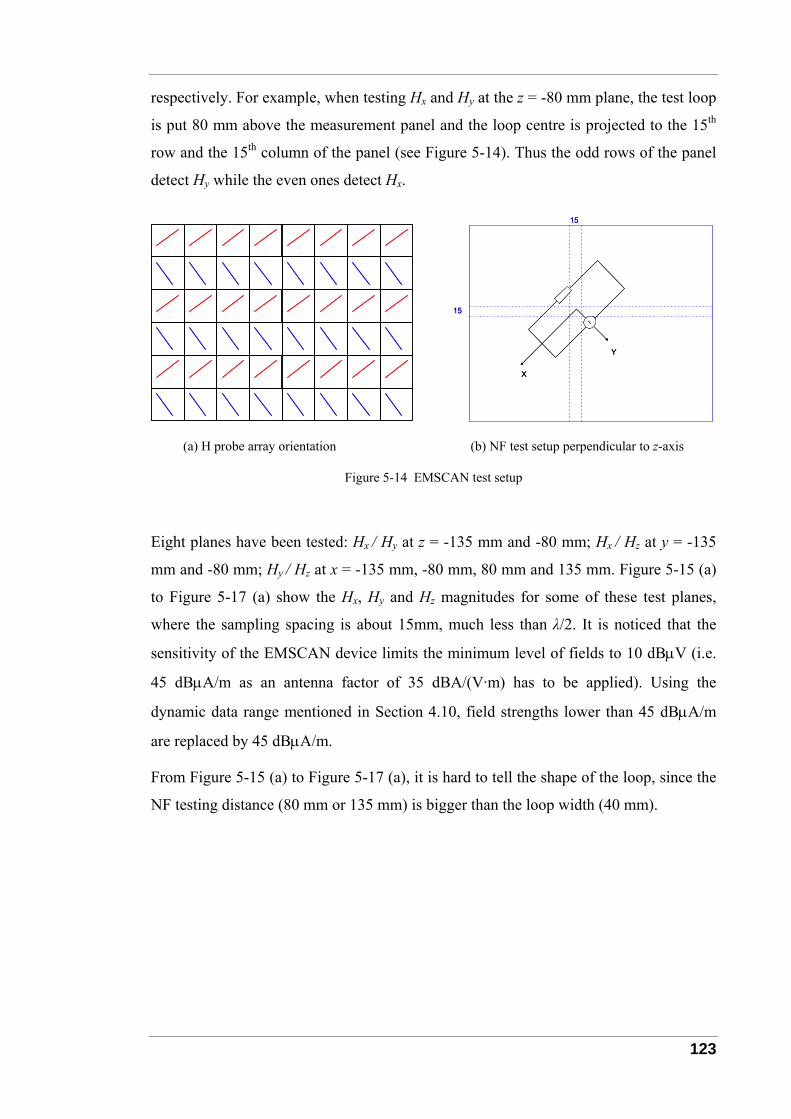
123

respectively. For example, when testing Hx and Hy at the z = -80 mm plane, the test loop

is put 80 mm above the measurement panel and the loop centre is projected to the 15th

row and the 15th column of the panel (see Figure 5-14). Thus the odd rows of the panel

detect Hy while the even ones detect Hx.

X

Y

~15

15

X

Y

~~15

15

(a) H probe array orientation (b) NF test setup perpendicular to z-axis

Figure 5-14 EMSCAN test setup

Eight planes have been tested: Hx / Hy at z = -135 mm and -80 mm; Hx / Hz at y = -135

mm and -80 mm; Hy / Hz at x = -135 mm, -80 mm, 80 mm and 135 mm. Figure 5-15 (a)

to Figure 5-17 (a) show the Hx, Hy and Hz magnitudes for some of these test planes,

where the sampling spacing is about 15mm, much less than λ/2. It is noticed that the

sensitivity of the EMSCAN device limits the minimum level of fields to 10 dBμV (i.e.

45 dBμA/m as an antenna factor of 35 dBA/(V·m) has to be applied). Using the

dynamic data range mentioned in Section 4.10, field strengths lower than 45 dBμA/m

are replaced by 45 dBμA/m.

From Figure 5-15 (a) to Figure 5-17 (a), it is hard to tell the shape of the loop, since the

NF testing distance (80 mm or 135 mm) is bigger than the loop width (40 mm).

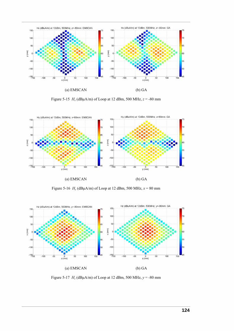
124

(a) EMSCAN (b) GA

Figure 5-15 Hx (dBμA/m) of Loop at 12 dBm, 500 MHz, z = -80 mm

(a) EMSCAN (b) GA

Figure 5-16 Hy (dBμA/m) of Loop at 12 dBm, 500 MHz, x = 80 mm

(a) EMSCAN (b) GA

Figure 5-17 Hz (dBμA/m) of Loop at 12 dBm, 500 MHz, y = -80 mm

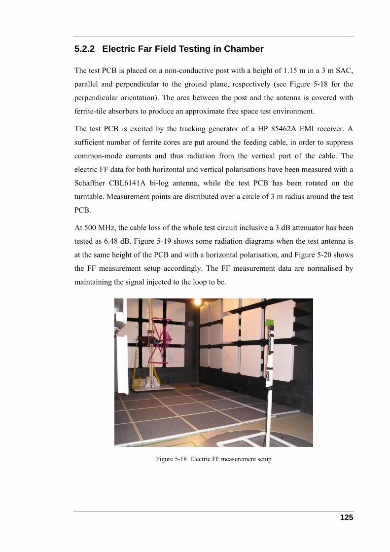
125

5.2.2 Electric Far Field Testing in Chamber

The test PCB is placed on a non-conductive post with a height of 1.15 m in a 3 m SAC,

parallel and perpendicular to the ground plane, respectively (see Figure 5-18 for the

perpendicular orientation). The area between the post and the antenna is covered with

ferrite-tile absorbers to produce an approximate free space test environment.

The test PCB is excited by the tracking generator of a HP 85462A EMI receiver. A

sufficient number of ferrite cores are put around the feeding cable, in order to suppress

common-mode currents and thus radiation from the vertical part of the cable. The

electric FF data for both horizontal and vertical polarisations have been measured with a

Schaffner CBL6141A bi-log antenna, while the test PCB has been rotated on the

turntable. Measurement points are distributed over a circle of 3 m radius around the test

PCB.

At 500 MHz, the cable loss of the whole test circuit inclusive a 3 dB attenuator has been

tested as 6.48 dB. Figure 5-19 shows some radiation diagrams when the test antenna is

at the same height of the PCB and with a horizontal polarisation, and Figure 5-20 shows

the FF measurement setup accordingly. The FF measurement data are normalised by

maintaining the signal injected to the loop to be.

Figure 5-18 Electric FF measurement setup

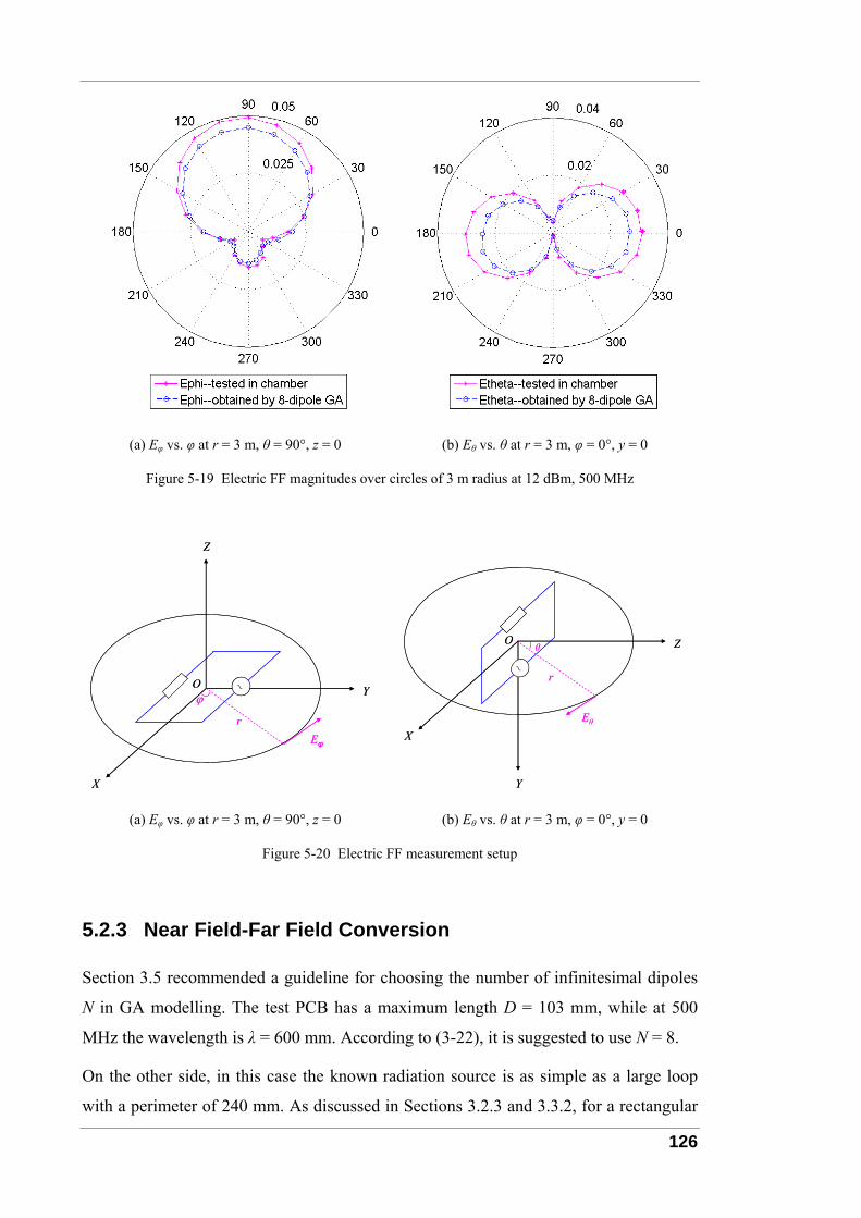
126

(a) Eφ vs. φ at r = 3 m, θ = 90°, z = 0 (b) Eθ vs. θ at r = 3 m, φ = 0°, y = 0

Figure 5-19 Electric FF magnitudes over circles of 3 m radius at 12 dBm, 500 MHz

X

Z

Yϕ

O ~

Eφ

r

X

Z

Yϕ

O ~

Eφ

r

X

Y

ZθO

~

Eθ

r

X

Y

ZθO

~

Eθ

r

(a) Eφ vs. φ at r = 3 m, θ = 90°, z = 0 (b) Eθ vs. θ at r = 3 m, φ = 0°, y = 0

Figure 5-20 Electric FF measurement setup

5.2.3 Near Field-Far Field Conversion

Section 3.5 recommended a guideline for choosing the number of infinitesimal dipoles

N in GA modelling. The test PCB has a maximum length D = 103 mm, while at 500

MHz the wavelength is λ = 600 mm. According to (3-22), it is suggested to use N = 8.

On the other side, in this case the known radiation source is as simple as a large loop

with a perimeter of 240 mm. As discussed in Sections 3.2.3 and 3.3.2, for a rectangular

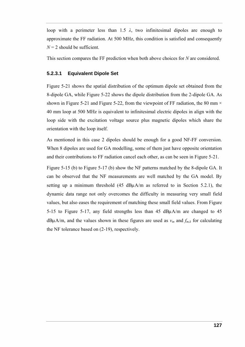
127

loop with a perimeter less than 1.5 λ, two infinitesimal dipoles are enough to

approximate the FF radiation. At 500 MHz, this condition is satisfied and consequently

N = 2 should be sufficient.

This section compares the FF prediction when both above choices for N are considered.

5.2.3.1 Equivalent Dipole Set

Figure 5-21 shows the spatial distribution of the optimum dipole set obtained from the

8-dipole GA, while Figure 5-22 shows the dipole distribution from the 2-dipole GA. As

shown in Figure 5-21 and Figure 5-22, from the viewpoint of FF radiation, the 80 mm ×

40 mm loop at 500 MHz is equivalent to infinitesimal electric dipoles in align with the

loop side with the excitation voltage source plus magnetic dipoles which share the

orientation with the loop itself.

As mentioned in this case 2 dipoles should be enough for a good NF-FF conversion.

When 8 dipoles are used for GA modelling, some of them just have opposite orientation

and their contributions to FF radiation cancel each other, as can be seen in Figure 5-21.

Figure 5-15 (b) to Figure 5-17 (b) show the NF patterns matched by the 8-dipole GA. It

can be observed that the NF measurements are well matched by the GA model. By

setting up a minimum threshold (45 dBμA/m as referred to in Section 5.2.1), the

dynamic data range not only overcomes the difficulty in measuring very small field

values, but also eases the requirement of matching these small field values. From Figure

5-15 to Figure 5-17, any field strengths less than 45 dBμA/m are changed to 45

dBμA/m, and the values shown in these figures are used as vm and fm,k for calculating

the NF tolerance based on (2-19), respectively.

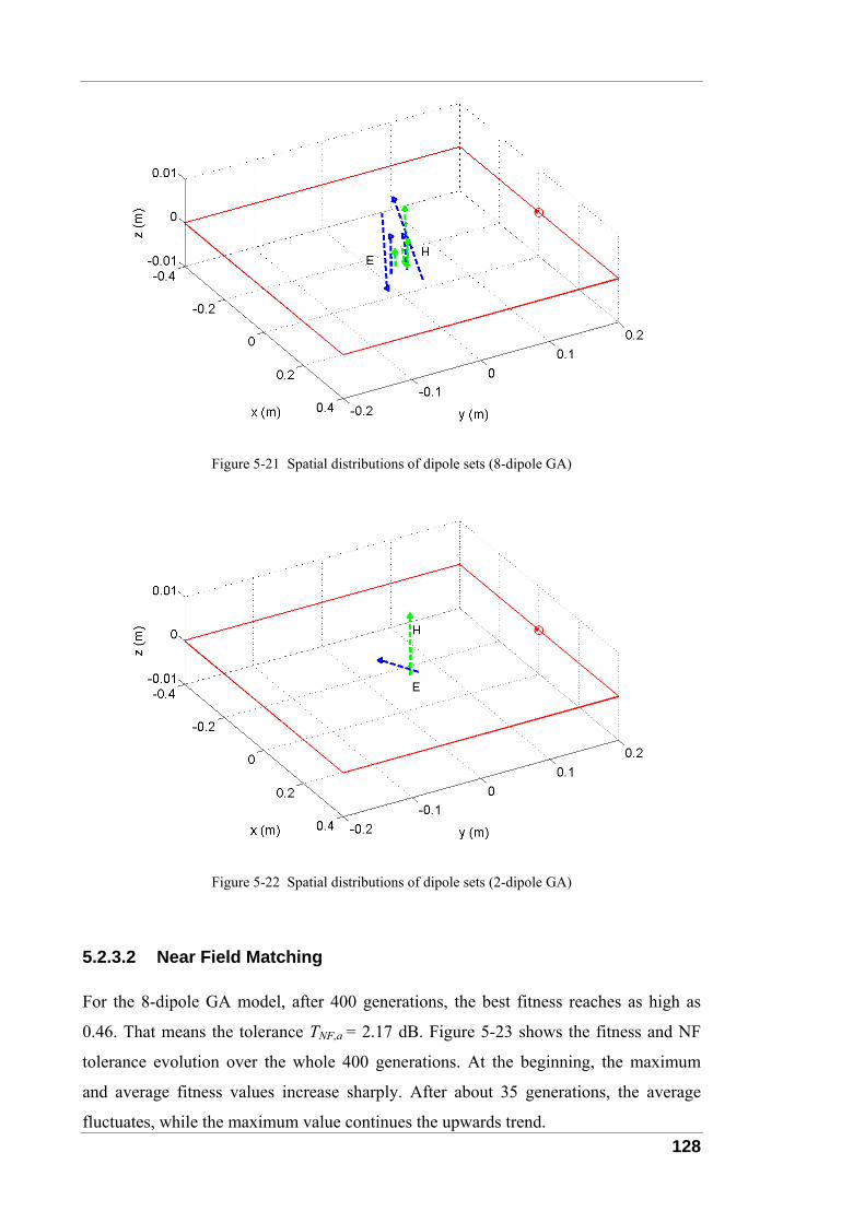
128

Figure 5-21 Spatial distributions of dipole sets (8-dipole GA)

Figure 5-22 Spatial distributions of dipole sets (2-dipole GA)

5.2.3.2 Near Field Matching

For the 8-dipole GA model, after 400 generations, the best fitness reaches as high as

0.46. That means the tolerance TNF,a = 2.17 dB. Figure 5-23 shows the fitness and NF

tolerance evolution over the whole 400 generations. At the beginning, the maximum

and average fitness values increase sharply. After about 35 generations, the average

fluctuates, while the maximum value continues the upwards trend.

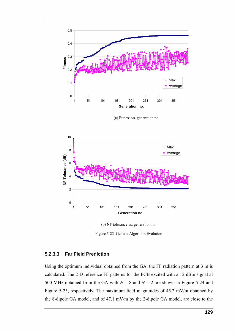
129

0

0.1

0.2

0.3

0.4

0.5

1 51 101 151 201 251 301 351

Generation no.

Fitn

ess

MaxAverage

(a) Fitness vs. generation no.

0

2

4

6

8

10

1 51 101 151 201 251 301 351

Generation no.

NF

Tole

ranc

e (d

B)

MaxAverage

(b) NF tolerance vs. generation no.

Figure 5-23 Genetic Algorithm Evolution

5.2.3.3 Far Field Prediction

Using the optimum individual obtained from the GA, the FF radiation pattern at 3 m is

calculated. The 2-D reference FF patterns for the PCB excited with a 12 dBm signal at

500 MHz obtained from the GA with N = 8 and N = 2 are shown in Figure 5-24 and

Figure 5-25, respectively. The maximum field magnitudes of 45.2 mV/m obtained by

the 8-dipole GA model, and of 47.1 mV/m by the 2-dipole GA model, are close to the

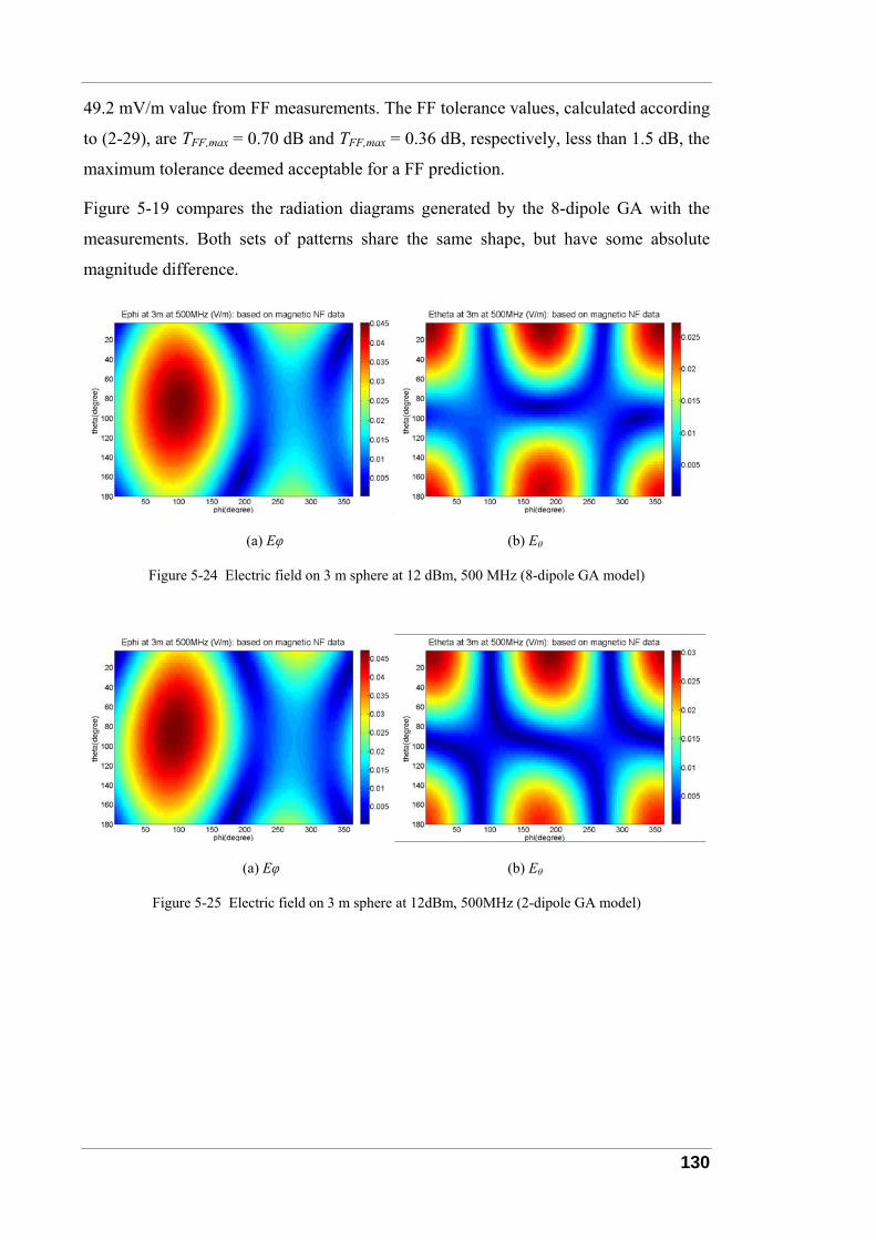
130

49.2 mV/m value from FF measurements. The FF tolerance values, calculated according

to (2-29), are TFF,max = 0.70 dB and TFF,max = 0.36 dB, respectively, less than 1.5 dB, the

maximum tolerance deemed acceptable for a FF prediction.

Figure 5-19 compares the radiation diagrams generated by the 8-dipole GA with the

measurements. Both sets of patterns share the same shape, but have some absolute

magnitude difference.

(a) Eφ (b) Eθ

Figure 5-24 Electric field on 3 m sphere at 12 dBm, 500 MHz (8-dipole GA model)

(a) Eφ (b) Eθ

Figure 5-25 Electric field on 3 m sphere at 12dBm, 500MHz (2-dipole GA model)

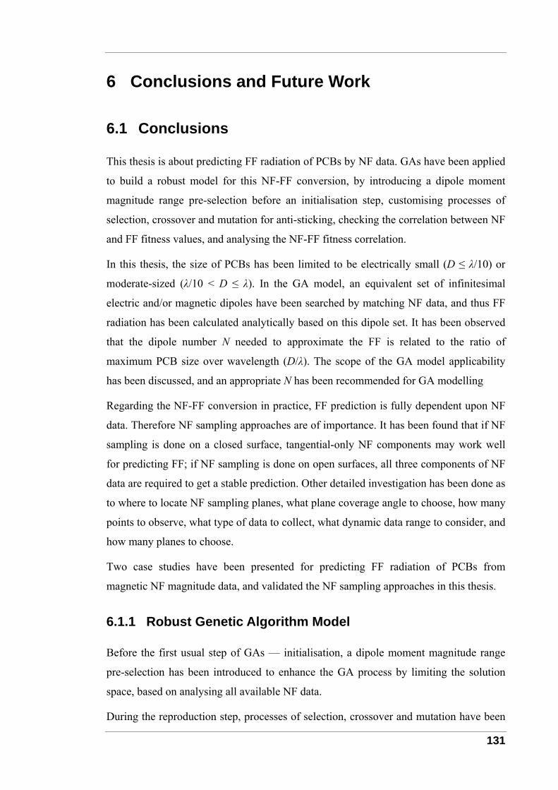
131

6 Conclusions and Future Work

6.1 Conclusions

This thesis is about predicting FF radiation of PCBs by NF data. GAs have been applied

to build a robust model for this NF-FF conversion, by introducing a dipole moment

magnitude range pre-selection before an initialisation step, customising processes of

selection, crossover and mutation for anti-sticking, checking the correlation between NF

and FF fitness values, and analysing the NF-FF fitness correlation.

In this thesis, the size of PCBs has been limited to be electrically small (D ≤ λ/10) or

moderate-sized (λ/10 < D ≤ λ). In the GA model, an equivalent set of infinitesimal

electric and/or magnetic dipoles have been searched by matching NF data, and thus FF

radiation has been calculated analytically based on this dipole set. It has been observed

that the dipole number N needed to approximate the FF is related to the ratio of

maximum PCB size over wavelength (D/λ). The scope of the GA model applicability

has been discussed, and an appropriate N has been recommended for GA modelling

Regarding the NF-FF conversion in practice, FF prediction is fully dependent upon NF

data. Therefore NF sampling approaches are of importance. It has been found that if NF

sampling is done on a closed surface, tangential-only NF components may work well

for predicting FF; if NF sampling is done on open surfaces, all three components of NF

data are required to get a stable prediction. Other detailed investigation has been done as

to where to locate NF sampling planes, what plane coverage angle to choose, how many

points to observe, what type of data to collect, what dynamic data range to consider, and

how many planes to choose.

Two case studies have been presented for predicting FF radiation of PCBs from

magnetic NF magnitude data, and validated the NF sampling approaches in this thesis.

6.1.1 Robust Genetic Algorithm Model

Before the first usual step of GAs — initialisation, a dipole moment magnitude range

pre-selection has been introduced to enhance the GA process by limiting the solution

space, based on analysing all available NF data.

During the reproduction step, processes of selection, crossover and mutation have been

132

customised for anti-sticking according to our practical situation, and thus improving the

robustness and repeatability of GAs.

Different fitness definitions for NF matching and FF prediction have been compared,

and the correlation between NF and FF fitness has been analysed.

Evolution of some genes and NF-FF fitness correlation has been illustrated, which helps

understand how the GA works in the NF-FF conversion.

6.1.2 Number of Infinitesimal Dipoles

FF behaviour of a long wire and a large loop in free space has been decomposed

analytically. It has been found from theoretical grounds that with respect to FF radiation,

these typical sources can be approximated by a few infinitesimal dipoles.

The GA has been applied to reconstruct the FF patterns of a long wire, a large loop and

a power-ground plane pair. The tolerance results and computational cost have been

investigated for different choices for the number of dipoles N in the GA model.

Correlation between N needed by the GA and the ratio of PCB size over wavelength

(D/λ) has been discussed. For electrically small PCBs (D ≤ λ/10), N = 2 has been

suggested; while for electrically moderate-sized PCBs (λ/10 < D ≤ λ), N = 8 has been

recommended; for D > λ, the GA model may not guarantee to approximate the FF

radiation with accuracy, due to the limitation for GAs to tackle too many unknowns.

6.1.3 Near Field Sampling Approaches

For predicting FF radiation of PCBs based on NF data by the GA model, it is important

to consider a location margin for the equivalent dipole set which is a little bigger than

the PCB physical size. This methodology may help reconstructing some characteristics

of the radiation PCB, such as radiation asymmetry due to finite ground plane, ground

plane splitting etc. In this thesis 5 mm is recommended as the optimum margin for a 90

mm × 60 mm PCB.

If NF sampling is done on closed surfaces, tangential magnetic NF components may be

enough for FF determination; otherwise the availability of the normal field components

can improve the results. Furthermore, for planar sampling on an open surface, plane

coverage angle θ is important for obtaining stable NF-FF conversion results. It is found

that θ > 60˚ can reach good repeatability for the FF prediction.

133

The number of observation points should be more than the number of unknown genes

for getting stable GA results. For a GA model with dipole number N = 8 (64 unknowns),

it is suggested to choose 100 observation points per sampling plane, and less than half

wavelength (λ/2) for the sampling spacing on the plane.

Regarding the number of sampling planes on each side of the x-y plane, 2 planes are

better than 1 plane, but 3 planes do not improve the results always. For the distance

between two sampling planes, there is no strict rule from the Nyquist sampling theorem

[54], while it is suggested to be around λ/2.

A new data process called dynamic data range (adyn) similar to the range of

measurement equipment has been introduced to NF-FF conversion. Among all NF

observation points, the maximum field value vmax is found. Field values smaller than

vmax - adyn enter into the GA process with the values replaced by vmax - adyn. In the

example presented in this thesis, adyn = 40 dB obtains the most stable FF prediction

based on NF data.

6.1.4 Near Field-Far Field Conversion Case Studies

Compared with the reactive NF region, the radiating NF region is better for converting

the NF data to FF radiation. This has been validated by simulated NF data from a

microstrip trace above an infinite ground plane, and also by NF measurements from an

electrically large loop in free space.

Magnetic NF magnitudes (Hx, Hy and Hz) on two planes are sufficient for NF-FF

conversion, if the plane coverage angle is big enough and also there are enough

sampling points. If tangential-only NF components are measured, NF data along the

lateral sides of PCBs are also needed for NF-FF conversion.

6.2 Future Work

6.2.1 Image Processing for Far Field Pattern Comparison

In Section 2.5.2.2, when evaluating whether a FF radiation prediction is good or not,

TFF,a and TFF,max were defined to check the tolerances between the FF prediction and the

reference values. TFF,a has compared the field differences at all FF observation points

one by one and later summarised them in an average manner, and TFF,max has compared

134

the maximum field magnitude among all points. However, whether this maximum value

happens at the same point has not been considered

FF pattern recognition and comparison could be improved by introducing image process

algorithms, especially when two patterns have similar shape but are not quite aligned.

6.2.2 Near Field Test Probe Array

Currently, there are two types of commercial NF scanners. One is magnetic scanners for

testing Hx and Hy components by a probe array at very short distances such as the

EMSCAN [58] device, the other is field scanners with a single electric/magnetic probe

moving together with a 3-D automatic location system such as the Detectus AB EMC-

Scanner [59].

For the convenience of predicting FF radiation based on NF measurements, it is

suggested to design a NF test probe array which combines both advantages of the above

scanners, i.e. making accurate 3-axis field measurements within a reasonable distance

from a test PCB (e.g. in the radiating NF region).

6.3 Outlook

In this thesis, most of NF sampling data have been obtained from electromagnetic field

simulations. In future, it will be necessary to apply the NF-FF conversion technique to

real-world electronic products, and to validate and fine-tune the GA parameters

discussed in Chapter 2 and the sampling guidelines in Chapter 4.

In Chapter 4 influence of NF sampling distance at low frequencies (< 300 MHz) on the

NF-FF conversion has been presented for one PCB example. Further investigation on

decreasing the NF testing distance from the order of 1 m to the order of 0.1 m while

maintaining the NF-FF conversion outcome at the same level would be of practical

interest.

Other extension to the work covered in this thesis could be source modelling of PCBs

with asymmetrical NF and symmetrical FF radiation patterns, and estimating FF fitness

based on NF fitness.

135

Appendix A Glossary

A.1 Abbreviations CISPR Special International Committee on Radio Interference

DUT Device Under Test

EMC Electromagnetic Compatibility

FCC Federal Communications Commission

FEM Finite Element Method

FF Far Field

GA Genetic Algorithm

MoM Method of Moments

NF Near Field

OATS Open Area Test Site

PCB Printed Circuit Board

SAC Semi-Anechoic Chamber

SLSI Super Large Scale Integrated

TEM Transverse Electromagnetic

TM Transverse Mangetic

2-D 2-Dimenional

3-D 3-dimensional

A.2 Symbols and Parameters ∇ Del vector operator

⋅ Dot product or multiplication

× Cross product or multiplication

∂ Partial derivative

V

dv∫∫∫ Integral on volume V

Letter in bold Vector

136

a radius (m)

adyn Dynamic range (dB)

an Normal unit vector

ar, ar’ Unit vector in the radius direction

au Unit vector

ax, ax’ Unit vector in the x- or x’-direction

ay, ay’ Unit vector in the y- or y’-direction

az, az’ Unit vector in the z- or z’-direction

aθ, aθ’ Unit vector in the elevation angle direction

aφ, aφ’ Unit vector in the azimuth angle direction

A, A Magnetic vector potential (Wb/m)

b System parameter for mutation

c Coefficient

Corr Correlation coefficient

d Distance (m)

dl Differential displacement

dv, dv’ Differential volume

D Length (m)

Dq qth dipole

E, E Electric field (V/m)

Emax Maximum electric field (V/m)

f Frequency (Hz)

f Wave spectrum function

F Individual Fitness

fm,k Field magnitude of kth individual at mth point (V/m or A/m)

g Generation number

G Maximum Generation Number

h Height (m)

H, H Magnetic field (A/m)

i Integer

I Current (A)

j Square root of -1, or integer

J Electric current density (A/m2)

k Integer

Kq Type of qth dipole

K Individual number in one population

137

l, l, l’, l’ Length (m)

L Length (m)

LB Lower domain bound

M Individual number in one sub-population

M Magnetic current density (V/ m2)

m Dipole moment magnitude (A·m or A·m2)

mq Moment magnitude of qth dipole (A·m or A·m2)

mE Electric dipole moment magnitude (A·m)

mM Magnetic dipole moment magnitude (A·m2)

N Dipole number, or sub-group number of individuals

Np Observation point number

nstick Stick counter

Pcross Crossover probability gip Parameter of ith individual at gth generation

Pmutate Mutation probability

q Dipole number

r, r, r’, r’, r” Radius in spherical coordinate (m)

R, R’ Length (m)

S Surface, or surface area (m2) gis ith individual at gth generation

sk kth individual

T Tolerance, or computation time

TNF Near field tolerance

TFF Far field tolerance

u random number from (0,1)

U Source voltage (V)

UB Upper domain bound

V Integration volume, or volume (m3)

W Width (m)

vm Field magnitude at mth observation point (V/m or A/m)

x, x’ Cartesian coordinate variable (m)

xq Location in Cartesian coordinate of qth dipole (m)

y, y’ Cartesian coordinate variable (m)

yq Location in Cartesian coordinate of qth dipole (m)

z, z’ Cartesian coordinate variable (m)

138

zq Location in Cartesian coordinate of qth dipole (m)

Zin Input impedance (Ω)

α Ratio factor, or angle (rad)

β Wave number (rad/m)

βq Moment phase of qth dipole (rad)

Γ Conversion matrix

δ Fractional deviation, or loss angle of medium

Δ Incremental change, or mutation step

ε Permittivity (F/m)

εr Relative permittivity

η Wave impedance (Ω)

θ, θ’, θ” Elevation angle in spherical coordinate (rad)

θq Elevation angle of qth dipole (rad)

λ Wavelength in propagating medium (m)

μ Permeability (H/m)

σ Conductivity (S/m)

φ, φ’, φ” Azimuth angle in spherical coordinate (rad)

φq Azimuth angle of qth dipole (rad)

ω Angular frequency (rad/s)

139

Appendix B List of Figures and Tables

B.1 List of Figures Figure 1-1 Original PCB radiation source and equivalent dipole set ..............................7

Figure 2-1 Location and orientation of dipole Dq ..........................................................14

Figure 2-2 GA flow chart: initialisation.........................................................................15

Figure 2-3 Fitness matrix for fine-tuning the dipole moment ranges ............................18

Figure 2-4 Fitness distribution vs maximum electric and magnetic dipole moments ...20

Figure 2-5 GA flow chart: reproduction ........................................................................21

Figure 2-6 Selection process for K individuals ..............................................................22

Figure 2-7 Linear crossover for real-coded genes..........................................................24

Figure 2-8 Mutation for real-coded genes......................................................................26

Figure 2-9 Spatial distribution of test and equivalent dipoles (solid: reference; dashed: GA)..................................................................................................................................29

Figure 2-10 Examples of correlation between NF and FF tolerances............................33

Figure 2-11 Mapping of electric FF patterns (field strength in dBmV/m) ....................36

Figure 2-12 Evolution in GA: “+”: Corr(TNF,a,TFF,max), “o”: Corr(TNF,a,TFF,a) .............37

Figure 2-13 Mapping of electric FF patterns (field strength in dBmV/m) ....................38

Figure 2-14 TNF,a vs. generation number........................................................................39

Figure 2-15 Spatial distribution of test and equivalent dipoles from 5 runs (solid: reference; dashed: GA) ...................................................................................................40

Figure 3-1 Radiation field from source with current density J(r’) and maximum dimension D ....................................................................................................................44

Figure 3-2 Centre-fed long wire.....................................................................................46

Figure 3-3 Approximate current distribution for thin, linear, centre-fed wire of various length...............................................................................................................................46

Figure 3-4 Current distribution for 0.5 m long wire at 300 MHz (D = λ/2) ..................47

Figure 3-5 Current distribution for 0.5 m long wire at 600 MHz (D = λ)......................47

Figure 3-6 Current distribution for 0.5 m long wire at 900 MHz (D = 3λ/2) ................48

Figure 3-7 Current distribution for 0.5 m long wire at 1.2 GHz (D = 2λ) .....................48

Figure 3-8 Current distribution for 0.5 m long wire at 1.5 GHz (D = 5λ/2) ..................49

140

Figure 3-9 Current distribution of a square loop with side length of L ......................... 52

Figure 3-10 Current distribution around 0.35 m × 0.35 m loop at 300 MHz ................ 52

Figure 3-11 Dipole parameters for approximating FF of 0.35 m × 0.35 m loop vs. frequency......................................................................................................................... 55

Figure 3-12 Input impedance of long wire at various frequencies ................................ 57

Figure 3-13 TFF,a vs. dipole number for 0.5 m long wire in free space.......................... 59

Figure 3-14 TFF,max vs. dipole number for 0.5 m long wire in free space....................... 59

Figure 3-15 FF pattern of 0.5 m long wire at 300MHz ................................................. 62

Figure 3-16 FF pattern of 0.5 m long wire at 600MHz ................................................. 63

Figure 3-17 FF pattern of 0.5 m long wire at 900MHz ................................................. 63

Figure 3-18 FF pattern of 0.5 m long wire at 1.2GHz ................................................... 63

Figure 3-19 FF pattern of 0.5 m long wire at 1.5GHz (left: 3-D; right: 2-D)................ 64

Figure 3-20 Spatial distribution of electric dipole set for 300 MHz, N = 1 ................... 65

Figure 3-21 Spatial distribution of electric dipole set for 600 MHz, N = 2 ................... 65

Figure 3-22 Spatial distribution of electric dipole set for 900 MHz, N = 3 ................... 65

Figure 3-23 Spatial distribution of electric dipole set for 1.2 GHz, N = 4..................... 66

Figure 3-24 Spatial distribution of electric dipole set for 1.5 GHz, N = 5..................... 66

Figure 3-25 Spatial distribution of equivalent dipole sets for 0.35 m × 0.35 m loop at 300MHz (solid: calculated; dashed: GA)........................................................................68

Figure 3-26 Radiation diagrams for 0.35 m × 0.35 m loop at 300 MHz (soild: reference; dotted: analytical calculation; dashed: GA; polar coordinate range: 0 – 30 dBmV/m)..68

Figure 3-27 Rectangular power-ground plane pair ........................................................ 69

Figure 3-28 Input impedance of power-ground plane pair at various frequencies ........ 71

Figure 3-29 TFF,a vs. dipole number for power-ground plane pair at various frequencies......................................................................................................................................... 72

Figure 3-30 TFF,max vs. dipole number for power-ground plane pair at various frequencies ...................................................................................................................... 72

Figure 3-31 Horizontal radiation diagrams (Emax vs. φ at θ = 90º) ................................ 73

Figure 3-32 Meshing of rectangular electrically moderate-sized PCB based on D/λ .... 76

Figure 4-1 PCB with finite ground plane....................................................................... 80

Figure 4-2 One-domain consideration for equivalent dipole set ...................................81

Figure 4-3 Input impedance of PCB with finite ground plane....................................... 81

Figure 4-4 NF and FF regions of PCB with finite ground plane ................................... 83

141

Figure 4-5 Magnetic NF Hx data at 125 MHz................................................................88

Figure 4-6 Magnetic NF Hy data at 125 MHz................................................................88

Figure 4-7 Magnetic NF Hz data at 125 MHz ................................................................88

Figure 4-8 Plane coverage angle θ for planar sampling.................................................93

Figure 4-9 FF pattern of PCB with finite ground plane at 125 MHz.............................94

Figure 4-10 Vertical and horizontal FF radiation pattern at 125 MHz, 3 m with N = 2 (soild: reference; dashed: GA; polar coordinate range: 0 – 40 dBmV/m) ......................95

Figure 4-11 TFF,a vs. TNF,a at 125 MHz with different numbers (Np) of points sampled at z = ± 200 mm ..................................................................................................................98

Figure 4-12 TFF,a vs. dipole number for PCB with finite ground plane at various frequencies ....................................................................................................................102

Figure 4-13 TFF,max vs. dipole number for PCB with finite ground plane at various frequencies ....................................................................................................................102

Figure 4-14 FF pattern of PCB with finite ground plane at 1 GHz .............................103

Figure 4-15 Vertical and horizontal FF radiation pattern at 1 GHz, 3 m with N = 8 (soild: reference; dashed: GA; polar coordinate range: 0 – 20 dBmV/m) ....................103

Figure 4-16 FF pattern of PCB with finite ground plane at 2 GHz .............................104

Figure 4-17 Vertical and horizontal FF radiation pattern at 2 GHz, 3 m with N = 8 (soild: reference; dashed: GA; polar coordinate range: 0 – 40 dBmV/m) ....................104

Figure 4-18 FF pattern of PCB with finite ground plane at 3 GHz .............................105

Figure 4-19 Vertical and horizontal FF radiation pattern at 3 GHz, 3 m with N = 8 (soild: reference; dashed: GA; polar coordinate range: 0 – 40 dBmV/m) ....................105

Figure 4-20 NF observation points for case #7............................................................108

Figure 4-21 Comparison of NF Hx with 40 dB dynamic data range............................109

Figure 4-22 Comparison of NF Hy with 40 dB dynamic data range............................109

Figure 4-23 Comparison of NF Hz with 40 dB dynamic data range............................110

Figure 4-24 Comparison of FF Emax with 40 dB dynamic data range..........................110

Figure 5-1 Microstrip trace on dielectric substrate ......................................................114

Figure 5-2 Ideal electric dipole above and perpendicular to a perfectly conducting ground plane..................................................................................................................115

Figure 5-3 Ideal electric dipole above and parallel to a perfectly conducting ground plane ..............................................................................................................................115

Figure 5-4 Equivalent model for PCB above infinite ground plane ............................116

Figure 5-5 Input impedance of microstrip trace above infinite ground plane..............117

Figure 5-6 NF and FF regions of microstrip trace on dielectric substrate ...................118

142

Figure 5-7 Magnetic NF Hx data of microstrip PCB at 1.2 GHz, z = 200 mm ............ 120

Figure 5-8 Magnetic NF Hy data of microstrip PCB at 1.2 GHz, z = 200 mm ............ 120

Figure 5-9 Magnetic NF Hz data of microstrip PCB at 1.2 GHz, z = 200 mm ............ 120

Figure 5-10 FF pattern of microstrip PCB at 300 MHz............................................... 121

Figure 5-11 FF pattern of microstrip PCB at 600 MHz............................................... 121

Figure 5-12 FF pattern of microstrip PCB at 900 MHz............................................... 121

Figure 5-13 FF pattern of microstrip PCB at 1.2 GHz ................................................ 122

Figure 5-14 EMSCAN test setup ................................................................................. 123

Figure 5-15 Hx (dBμA/m) of Loop at 12 dBm, 500 MHz, z = -80 mm ....................... 124

Figure 5-16 Hy (dBμA/m) of Loop at 12 dBm, 500 MHz, x = 80 mm ........................ 124

Figure 5-17 Hz (dBμA/m) of Loop at 12 dBm, 500 MHz, y = -80 mm ....................... 124

Figure 5-18 Electric FF measurement setup ................................................................125

Figure 5-19 Electric FF magnitudes over circles of 3 m radius at 12 dBm, 500 MHz 126

Figure 5-20 Electric FF measurement setup ................................................................126

Figure 5-21 Spatial distributions of dipole sets (8-dipole GA).................................... 128

Figure 5-22 Spatial distributions of dipole sets (2-dipole GA).................................... 128

Figure 5-23 Genetic Algorithm Evolution................................................................... 129

Figure 5-24 Electric field on 3 m sphere at 12 dBm, 500 MHz (8-dipole GA model) 130

Figure 5-25 Electric field on 3 m sphere at 12dBm, 500MHz (2-dipole GA model)..130

B.2 List of Tables Table 2-1 Three levels of mutation ................................................................................26

Table 2-2 Parameters of test and equivalent dipoles......................................................28

Table 2-3 NF and FF tolerances and correlation vs. fitness definition ..........................35

Table 2-4 Tolerance and correlation figures for 5 GA runs........................................... 39

Table 3-1 FF decomposition for wire of length D by analytical approximation ........... 50

Table 3-2 Electric and magnetic dipole parameters....................................................... 54

Table 3-3 Comparison between analytical and GA dipoles for 0.5 m long wire at 300 MHz ................................................................................................................................ 59

Table 3-4 Tolerances for analytical and GA solutions with K = 102, G = 200 ............. 60

Table 3-5 Comparison between analytical and GA dipoles for 0.5 m long wire at 1.5 GHz ................................................................................................................................. 62

143

Table 3-6 Dipole parameters for analytic and GA results at 300 MHz for 0.35 m × 0.35 m loop .............................................................................................................................68

Table 3-7 Tolerances for analytical and GA results at 300 MHz ..................................69

Table 3-8 Resonance frequency points for TM modes ..................................................70

Table 3-9 Computation time with both electric and magnetic dipoles searched in GA model...............................................................................................................................75

Table 4-1 NF sampling cases for PCB with finite ground plane ...................................84

Table 4-2 FF tolerances with varying dipole location margins at 125 MHz .................86

Table 4-3 FF tolerances with varying dipole location margins at 1 GHz ......................86

Table 4-4 FF tolerances with varying dipole location margins at 2 GHz ......................87

Table 4-5 FF tolerances with varying dipole location margins at 3 GHz ......................87

Table 4-6 FF tolerances with varying sampling distances at 125 MHz.........................90

Table 4-7 FF tolerances with varying sampling distances at 1 GHz .............................90

Table 4-8 FF tolerances with varying sampling distances at 2 GHz .............................91

Table 4-9 FF tolerances with varying sampling distances at 3 GHz .............................91

Table 4-10 FF tolerances with varying plane coverage angles at 125 MHz..................94

Table 4-11 FF tolerances with varying data types at 125 MHz .....................................96

Table 4-12 FF tolerances with varying numbers of observation points at 125 MHz.....97

Table 4-13 FF tolerances with varying numbers of sampling planes at 1 GHz.............99

Table 4-14 FF tolerances with varying numbers of sampling planes at 2 GHz.............99

Table 4-15 FF tolerances with varying numbers of sampling planes at 3 GHz...........100

Table 4-16 FF tolerances with NF sampled at z = ± 75, 200 mm (case #7) at 2 GHz.101

Table 4-17 NF-FF tolerances and correlation with varying dynamic data ranges.......107

Table 5-1 Parameters of image dipole below the ground plane...................................116

Table 5-2 NF and FF tolerances with different NF sampling planes...........................119

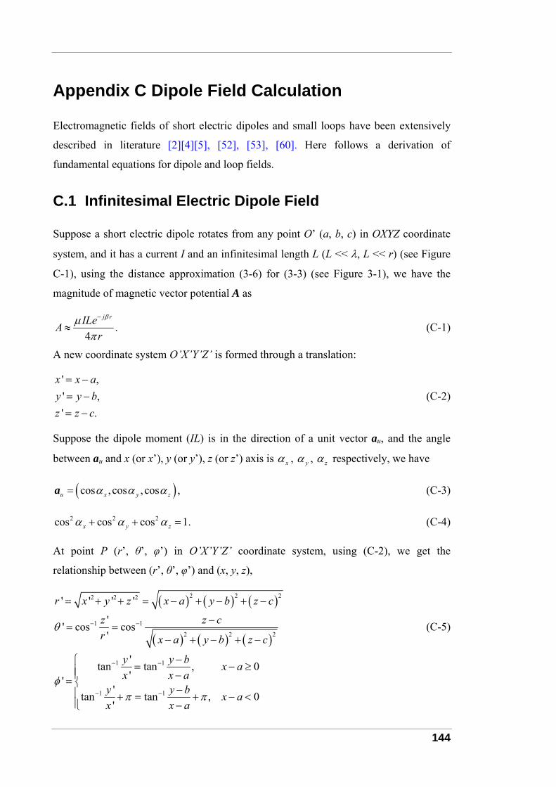
144

Appendix C Dipole Field Calculation

Electromagnetic fields of short electric dipoles and small loops have been extensively

described in literature [2][4][5], [52], [53], [60]. Here follows a derivation of

fundamental equations for dipole and loop fields.

C.1 Infinitesimal Electric Dipole Field

Suppose a short electric dipole rotates from any point O’ (a, b, c) in OXYZ coordinate

system, and it has a current I and an infinitesimal length L (L << λ, L << r) (see Figure

C-1), using the distance approximation (3-6) for (3-3) (see Figure 3-1), we have the

magnitude of magnetic vector potential A as

.4

j rILeAr

βμπ

−

≈ (C-1)

A new coordinate system O’X’Y’Z’ is formed through a translation:

' ,' ,' .

x x ay y bz z c

= −= −= −

(C-2)

Suppose the dipole moment (IL) is in the direction of a unit vector au, and the angle

between au and x (or x’), y (or y’), z (or z’) axis is xα , yα , zα respectively, we have

( )cos ,cos ,cos ,u x y zα α α=a (C-3)

2 2 2cos cos cos 1.x y zα α α+ + = (C-4)

At point P (r’, θ’, φ’) in O’X’Y’Z’ coordinate system, using (C-2), we get the

relationship between (r’, θ’, φ’) and (x, y, z),

( ) ( ) ( )

( ) ( ) ( )

2 2 22 2 2

1 1

2 2 2

1 1

1 1

' ' ' '

'' cos cos'

'tan tan , 0''

'tan tan , 0'

r x y z x a y b z c

z z cr x a y b z c

y y b x ax x a

y y b x ax x a

θ

φπ π

− −

− −

− −

= + + = − + − + −

−= =

− + − + −

−⎧ = − ≥⎪⎪ −= ⎨ −⎪ + = + − <⎪ −⎩

(C-5)

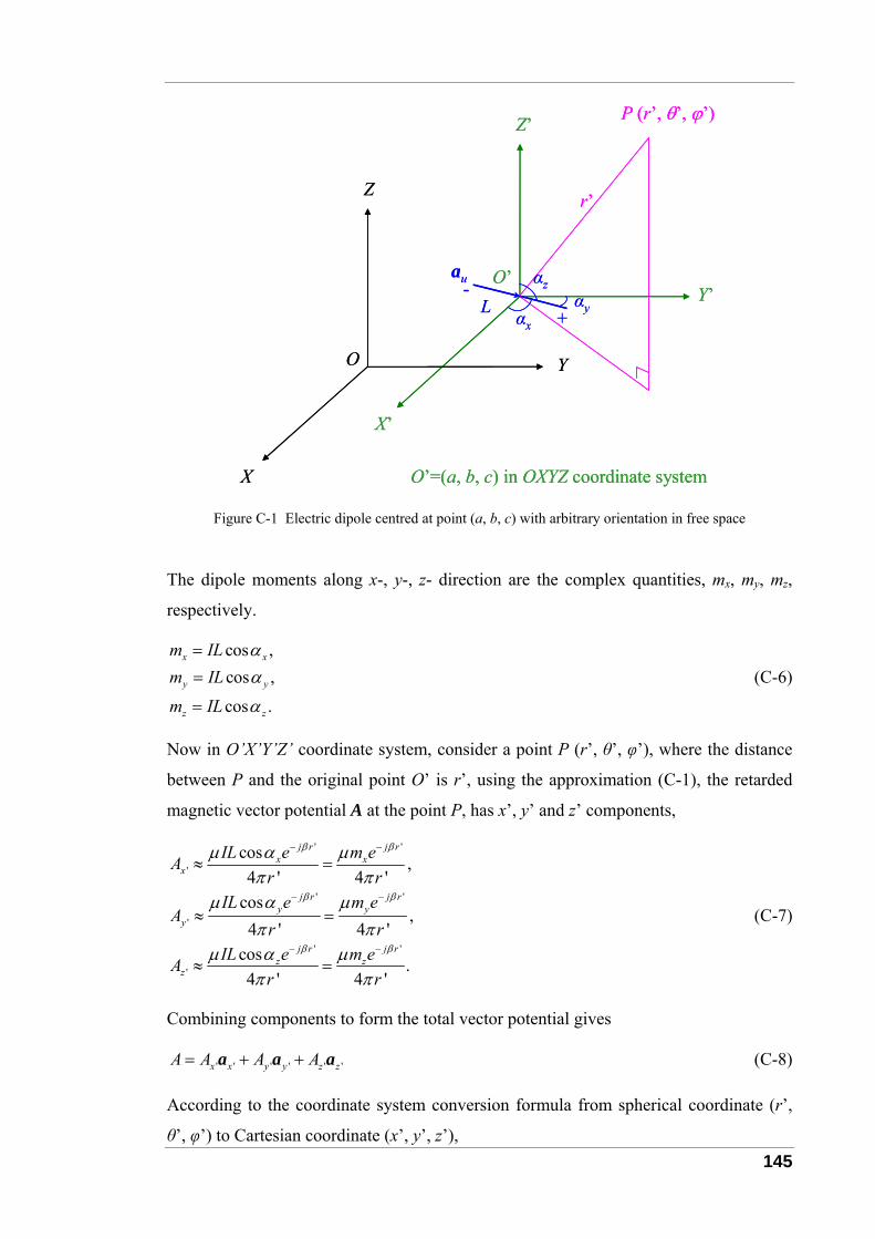
145

X’

Z’

Y’

P (r’, θ’, ϕ’)

L

r’

O’

αx

αzαy

au

X

Y

Z

O

O’=(a, b, c) in OXYZ coordinate system

+-

X’

Z’

Y’

P (r’, θ’, ϕ’)

L

r’

O’

αx

αzαy

au

X

Y

Z

O

O’=(a, b, c) in OXYZ coordinate system

+-

Figure C-1 Electric dipole centred at point (a, b, c) with arbitrary orientation in free space

The dipole moments along x-, y-, z- direction are the complex quantities, mx, my, mz,

respectively.

cos ,cos ,

cos .

x x

y y

z z

m ILm IL

m IL

αα

α

=

=

=

(C-6)

Now in O’X’Y’Z’ coordinate system, consider a point P (r’, θ’, φ’), where the distance

between P and the original point O’ is r’, using the approximation (C-1), the retarded

magnetic vector potential A at the point P, has x’, y’ and z’ components,

' '

'

' '

'

' '

'

cos ,4 ' 4 '

cos,

4 ' 4 'cos .4 ' 4 '

j r j rx x

x

j r j ry y

y

j r j rz z

z

IL e m eAr r

IL e m eA

r rIL e m eA

r r

β β

β β

β β

μ α μπ π

μ α μπ π

μ α μπ π

− −

− −

− −

≈ =

≈ =

≈ =

(C-7)

Combining components to form the total vector potential gives

' ' ' ' ' 'x x y y z zA A A A= + +a a a (C-8)

According to the coordinate system conversion formula from spherical coordinate (r’,

θ’, φ’) to Cartesian coordinate (x’, y’, z’),

146

' ' ' '

' ' ' '

' ' '

sin 'cos ' cos 'cos ' sin ',

sin 'sin ' cos 'sin ' cos ',

cos ' sin ',

x r

y r

z r

θ ϕ

θ ϕ

θ

θ ϕ θ ϕ ϕ

θ ϕ θ ϕ ϕ

θ θ

= + −

= + +

= −

a a a a

a a a a

a a a

(C-9)

we get the components of A

( )

( )

' ' ' '

'

' ' ' '

'

' ' '

sin 'cos ' sin 'sin ' cos '

sin 'cos ' sin 'sin ' cos ' ,4 '

cos 'cos ' cos 'sin ' sin '

cos 'cos ' cos 'sin ' sin ' ,4 '

sin ' cos '

r x y z

j r

x y z

x y z

j r

x y z

j

x y

A A A A

e m m mr

A A A A

e m m mr

eA A A

β

θ

β

β

ϕ

θ ϕ θ ϕ θ

μ θ ϕ θ ϕ θπ

θ ϕ θ ϕ θ

μ θ ϕ θ ϕ θπ

μϕ ϕ

−

−

−

= + +

= + +

= + −

= + −

= − + = ( )'

sin ' cos ' .4 '

r

x ym mr

ϕ ϕπ

− +

(C-10)

We have the magnetic field according to

1μ

= ∇×H A, (C-11)

( )

( )

' ''

'''

'2

' ''

( sin ') ( )1 0,'sin ' ' '

( ' )1 1' sin ' ' '

1 1sin ' cos ' ,4 ' '

( ' )1' ' '

1 cos 'cos ' cos 'sin ' sin '4

r

r

j rx y

r

x y z

A AHr

r AAHr r

jm m er r

r A AHr r

jm m m

φ θ

φθ

β

θϕ

θμ θ θ ϕ

μ θ ϕ

βϕ ϕπ

μ θβθ ϕ θ ϕ θ

π

−

∂⎧ ⎫∂= − =⎨ ⎬∂ ∂⎩ ⎭

∂⎧ ⎫∂= −⎨ ⎬∂ ∂⎩ ⎭

⎛ ⎞= − + +⎜ ⎟⎝ ⎠

∂ ∂⎧ ⎫= −⎨ ⎬∂ ∂⎩ ⎭

= − − + '2

1 .' '

j rer r

β−⎛ ⎞+⎜ ⎟⎝ ⎠

(C-12)

Electric field is obtained according to

1 , ,j

μβ ω εμ ηωε ε

= ∇× = =E H, (C-13)

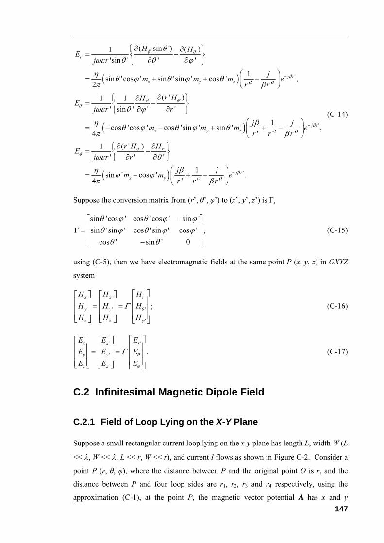
147

( )

( )

' ''

'2 3

'''

2 3

( sin ') ( )1'sin ' ' '

1sin 'cos ' sin 'sin ' cos ' ,2 ' '

( ' )1 1' sin ' ' '

1cos 'cos ' cos 'sin ' sin '4 ' ' '

r

j rx y z

r

x y z

H HEj r

jm m m er r

r HHEj r r

j jm m mr r r

φ θ

β

φθ

θωε θ θ ϕ

η θ ϕ θ ϕ θπ β

ωε θ ϕ

η βθ ϕ θ ϕ θπ β

−

∂⎧ ⎫∂= −⎨ ⎬∂ ∂⎩ ⎭

⎛ ⎞= + + −⎜ ⎟

⎝ ⎠∂⎧ ⎫∂

= −⎨ ⎬∂ ∂⎩ ⎭⎛

= − − + + −

( )

'

' ''

'2 3

,

( ' )1' ' '

1sin ' cos ' .4 ' ' '

j r

r

j rx y

e

r H HEj r r

j jm m er r r

β

θφ

β

ωε θ

η βϕ ϕπ β

−

−

⎞⎜ ⎟⎝ ⎠

∂ ∂⎧ ⎫= −⎨ ⎬∂ ∂⎩ ⎭⎛ ⎞

= − + −⎜ ⎟⎝ ⎠

(C-14)

Suppose the conversion matrix from (r’, θ’, φ’) to (x’, y’, z’) is Γ,

sin 'cos ' cos 'cos ' sin 'sin 'sin ' cos 'sin ' cos ' ,

cos ' sin ' 0

θ ϕ θ ϕ ϕθ ϕ θ ϕ ϕ

θ θ

−⎡ ⎤⎢ ⎥Γ = ⎢ ⎥⎢ ⎥−⎣ ⎦

(C-15)

using (C-5), then we have electromagnetic fields at the same point P (x, y, z) in OXYZ

system

' '

' '

' '

;x x r

y y

z z

H H HH H HH H H

θ

ϕ

Γ⎡ ⎤⎡ ⎤ ⎡ ⎤⎢ ⎥⎢ ⎥ ⎢ ⎥= = ⎢ ⎥⎢ ⎥ ⎢ ⎥⎢ ⎥⎢ ⎥ ⎢ ⎥⎣ ⎦ ⎣ ⎦ ⎣ ⎦

(C-16)

' '

' '

' '

.x x r

y y

z z

E E EE E EE E E

θ

ϕ

Γ⎡ ⎤⎡ ⎤ ⎡ ⎤⎢ ⎥⎢ ⎥ ⎢ ⎥= = ⎢ ⎥⎢ ⎥ ⎢ ⎥⎢ ⎥⎢ ⎥ ⎢ ⎥⎣ ⎦ ⎣ ⎦ ⎣ ⎦

(C-17)

C.2 Infinitesimal Magnetic Dipole Field

C.2.1 Field of Loop Lying on the X-Y Plane

Suppose a small rectangular current loop lying on the x-y plane has length L, width W (L

<< λ, W << λ, L << r, W << r), and current I flows as shown in Figure C-2. Consider a

point P (r, θ, φ), where the distance between P and the original point O is r, and the

distance between P and four loop sides are r1, r2, r3 and r4 respectively, using the

approximation (C-1), at the point P, the magnetic vector potential A has x and y

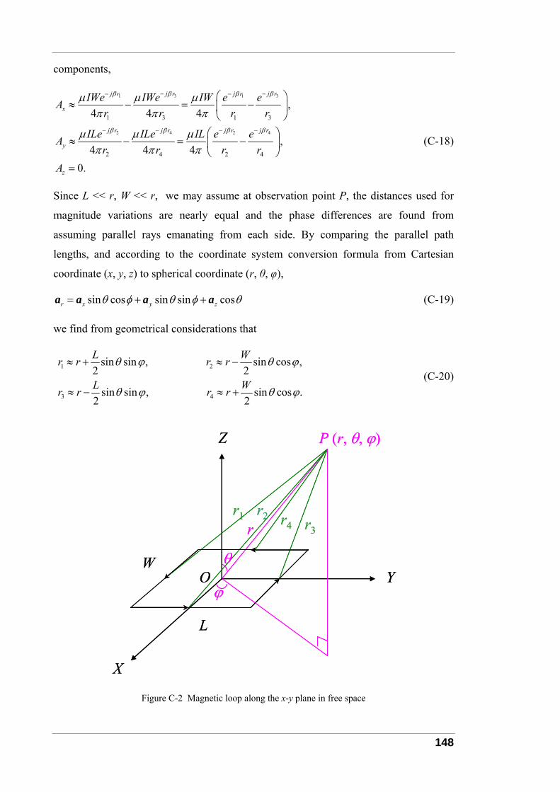
148

components,

3 31 1

2 4 2 4

1 3 1 3

2 4 2 4

,4 4 4

,4 4 4

0.

j r j rj r j r

x

j r j r j r j r

y

z

IWe IWe IW e eAr r r r

ILe ILe IL e eAr r r r

A

β ββ β

β β β β

μ μ μπ π π

μ μ μπ π π

− −− −

− − − −

⎛ ⎞≈ − = −⎜ ⎟

⎝ ⎠⎛ ⎞

≈ − = −⎜ ⎟⎝ ⎠

=

(C-18)

Since L << r, W << r, we may assume at observation point P, the distances used for

magnitude variations are nearly equal and the phase differences are found from

assuming parallel rays emanating from each side. By comparing the parallel path

lengths, and according to the coordinate system conversion formula from Cartesian

coordinate (x, y, z) to spherical coordinate (r, θ, φ),

sin cos sin sin cosr x y zθ φ θ φ θ= + +a a a a (C-19)

we find from geometrical considerations that

1 2

3 4

sin sin , sin cos ,2 2

sin sin , sin cos .2 2

L Wr r r r

L Wr r r r

θ ϕ θ ϕ

θ ϕ θ ϕ

≈ + ≈ −

≈ − ≈ + (C-20)

X

Z

Y

P (r, θ, ϕ)

W

L

rr1 r2

r3r4

θ

ϕO

X

Z

Y

P (r, θ, ϕ)

W

L

rr1 r2

r3r4

θ

ϕO

Figure C-2 Magnetic loop along the x-y plane in free space

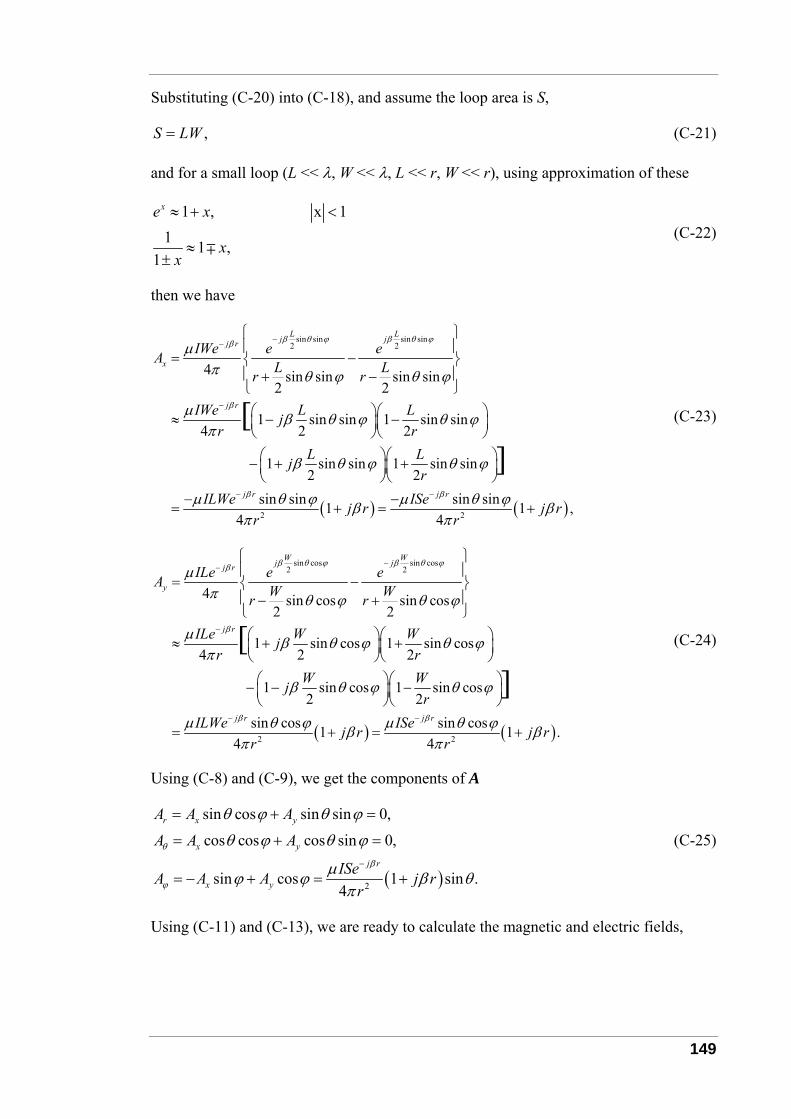
149

Substituting (C-20) into (C-18), and assume the loop area is S,

,S LW= (C-21)

and for a small loop (L << λ, W << λ, L << r, W << r), using approximation of these

1 , x 11 1 ,

1

xe x

xx

≈ + <

≈±

∓ (C-22)

then we have

sin sin sin sin2 2

4 sin sin sin sin2 2

1 sin sin 1 sin sin4 2 2

1 sin sin 1 sin sin2 2

si

[]

L Lj jj r

x

j r

j r

IWe e eA L Lr r

IWe L Ljr r

L Ljr

ILWe

β θ ϕ β θ ϕβ

β

β

μπ θ ϕ θ ϕ

μ β θ ϕ θ ϕπ

β θ ϕ θ ϕ

μ

−−

−

−

⎧ ⎫⎪ ⎪

= −⎨ ⎬⎪ ⎪+ −⎩ ⎭

⎛ ⎞⎛ ⎞≈ − −⎜ ⎟⎜ ⎟⎝ ⎠⎝ ⎠⎛ ⎞⎛ ⎞− + +⎜ ⎟⎜ ⎟⎝ ⎠⎝ ⎠

−= ( ) ( )2 2

n sin sin sin1 1 ,4 4

j rISej r j rr r

βθ ϕ μ θ ϕβ βπ π

−−+ = +

(C-23)

sin cos sin cos2 2

4 sin cos sin cos2 2

1 sin cos 1 sin cos4 2 2

1 sin cos 1 sin cos2 2

sin

[]

W Wj jj r

y

j r

j r

ILe e eA W Wr r

ILe W Wjr r

W Wjr

ILWe

β θ ϕ β θ ϕβ

β

β

μπ θ ϕ θ ϕ

μ β θ ϕ θ ϕπ

β θ ϕ θ ϕ

μ θ

−−

−

−

⎧ ⎫⎪ ⎪

= −⎨ ⎬⎪ ⎪− +⎩ ⎭

⎛ ⎞⎛ ⎞≈ + +⎜ ⎟⎜ ⎟⎝ ⎠⎝ ⎠⎛ ⎞⎛ ⎞− − −⎜ ⎟⎜ ⎟⎝ ⎠⎝ ⎠

= ( ) ( )2 2

cos sin cos1 1 .4 4

j rISej r j rr r

βϕ μ θ ϕβ βπ π

−

+ = +

(C-24)

Using (C-8) and (C-9), we get the components of A

( )2

sin cos sin sin 0,

cos cos cos sin 0,

sin cos 1 sin .4

r x y

x y

j r

x y

A A A

A A A

ISeA A A j rr

θ

β

ϕ

θ ϕ θ ϕ

θ ϕ θ ϕ

μϕ ϕ β θπ

−

= + =

= + =

= − + = +

(C-25)

Using (C-11) and (C-13), we are ready to calculate the magnetic and electric fields,

150

2 3

2 3

( sin ) ( )1 1cos ,sin 2

( )1 1 1sin ,sin 4

( )1 0;

j rr

j rr

r

A A j IS jH er r r

rAA j IS j jH er r r r r

rA AHr r

ϕ βθ

ϕ βθ

θϕ

θ β θμ θ θ ϕ π β

β βθμ θ ϕ π β

μ θ

−

−

∂⎧ ⎫∂ ⎛ ⎞= − = −⎨ ⎬ ⎜ ⎟∂ ∂ ⎝ ⎠⎩ ⎭

∂⎧ ⎫ ⎛ ⎞∂= − = + −⎨ ⎬ ⎜ ⎟∂ ∂ ⎝ ⎠⎩ ⎭

∂ ∂⎧ ⎫= − =⎨ ⎬∂ ∂⎩ ⎭

(C-26)

2

( sin ) ( )1 0,sin

( )1 1 0,sin

( )1 1sin .4

r

r

j rr

H HEj r

rHHEj r r

rH H j IS jE ej r r r r

ϕ θ

ϕθ

βθϕ

θωε θ θ ϕ

ωε θ ϕ

ωμ βθωε θ π

−

∂⎧ ⎫∂= − =⎨ ⎬∂ ∂⎩ ⎭

∂⎧ ⎫∂= − =⎨ ⎬∂ ∂⎩ ⎭

∂ ∂ −⎧ ⎫ ⎛ ⎞= − = +⎨ ⎬ ⎜ ⎟∂ ∂ ⎝ ⎠⎩ ⎭

(C-27)

C.2.2 Field of Loop Lying on the Y-Z Plane

Suppose a small rectangular current loop lying on the y-z plane has length L and width

W (L << λ, W << λ, L << r, W << r), and current I flows as shown in Figure C-3. Using

the approximation (C-1), the magnetic vector potential A at a point P (r, θ, φ), has y-

and z- components,

Using (C-19), we find a similar distance approximation as follows:

1 2

3 4

sin sin , cos ,2 2

sin sin , cos .2 2

L Wr r r r

L Wr r r r

θ ϕ θ

θ ϕ θ

≈ + ≈ +

≈ − ≈ − (C-28)

Substituting (C-28) into (C-18), and using (C-21) and (C-22), we have

( )

cos cos2 2

2 2

4 cos cos2 2

1 cos 1 cos4 2 2

1 cos 1 cos2 2

cos cos1 14 4

[]

W Wj jj r

y

j r

j r j r

ILe e eA W Wr r

ILe W Wjr r

W Wjr

ILWe ISej r jr r

β θ β θβ

β

β β

μπ θ θ

μ β θ θπ

β θ θ

μ θ μ θβ βπ π

−−

−

− −

⎧ ⎫⎪ ⎪

= −⎨ ⎬⎪ ⎪+ −⎩ ⎭

⎛ ⎞⎛ ⎞≈ − −⎜ ⎟⎜ ⎟⎝ ⎠⎝ ⎠⎛ ⎞⎛ ⎞− + +⎜ ⎟⎜ ⎟⎝ ⎠⎝ ⎠

− −= + = +( ) ,r

(C-29)

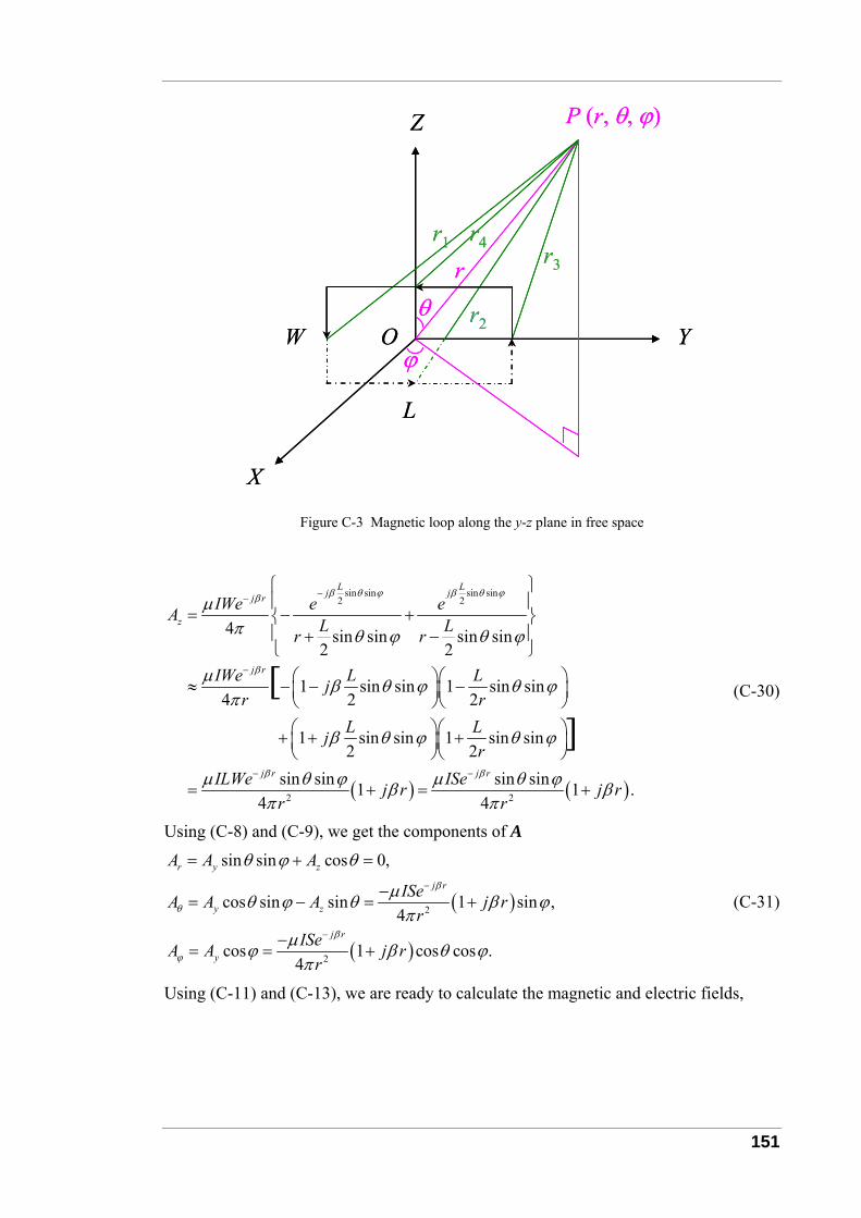
151

Z

Y

P (r, θ, ϕ)

W

L

rr1

r2

r3

r4

θ

ϕO

X

Z

Y

P (r, θ, ϕ)

W

L

rr1

r2

r3

r4

θ

ϕO

X

Figure C-3 Magnetic loop along the y-z plane in free space

sin sin sin sin2 2

4 sin sin sin sin2 2

1 sin sin 1 sin sin4 2 2

1 sin sin 1 sin sin2 2

s

[]

L Lj jj r

z

j r

j r

IWe e eA L Lr r

IWe L Ljr r

L Ljr

ILWe

β θ ϕ β θ ϕβ

β

β

μπ θ ϕ θ ϕ

μ β θ ϕ θ ϕπ

β θ ϕ θ ϕ

μ

−−

−

−

⎧ ⎫⎪ ⎪

= − +⎨ ⎬⎪ ⎪+ −⎩ ⎭

⎛ ⎞⎛ ⎞≈ − − −⎜ ⎟⎜ ⎟⎝ ⎠⎝ ⎠⎛ ⎞⎛ ⎞+ + +⎜ ⎟⎜ ⎟⎝ ⎠⎝ ⎠

= ( ) ( )2 2

in sin sin sin1 1 .4 4

j rISej r j rr r

βθ ϕ μ θ ϕβ βπ π

−

+ = +

(C-30)

Using (C-8) and (C-9), we get the components of A

( )

( )

2

2

sin sin cos 0,

cos sin sin 1 sin ,4

cos 1 cos cos .4

r y z

j r

y z

j r

y

A A A

ISeA A A j rr

ISeA A j rr

β

θ

β

ϕ

θ ϕ θ

μθ ϕ θ β ϕπ

μϕ β θ ϕπ

−

−

= + =

−= − = +

−= = +

(C-31)

Using (C-11) and (C-13), we are ready to calculate the magnetic and electric fields,

152

2 3

2 3

2 3

( sin ) ( )1 1sin cos ,sin 2

( )1 1 1cos cos ,sin 4

( )1 1sin4

j rr

j rr

jr

A A j IS jH er r r

rAA j IS j jH er r r r r

rA A j IS j jH er r r r r

ϕ βθ

φ βθ

βθϕ

θ β θ ϕμ θ θ ϕ π β

β βθ ϕμ θ ϕ π β

β βϕμ θ π β

−

−

−

∂⎧ ⎫∂ ⎛ ⎞= − = −⎨ ⎬ ⎜ ⎟∂ ∂ ⎝ ⎠⎩ ⎭

∂⎧ ⎫ ⎛ ⎞∂ −= − = + −⎨ ⎬ ⎜ ⎟∂ ∂ ⎝ ⎠⎩ ⎭

∂ ⎛ ⎞∂⎧ ⎫= − = + −⎨ ⎬ ⎜ ⎟∂ ∂⎩ ⎭ ⎝ ⎠;r

(C-32)

2

2

( sin ) ( )1 0,sin

( )1 1 1sin ,sin 4

( )1 1cos cos .4

r

j rr

j rr

H HEj r

rHH j IS jE ej r r r r

rH H j IS jE ej r r r r

ϕ θ

ϕ βθ

βθϕ

θωε θ θ ϕ

ωμ βϕωε θ ϕ π

ωμ βθ ϕωε θ π

−

−

∂⎧ ⎫∂= − =⎨ ⎬∂ ∂⎩ ⎭

∂⎧ ⎫∂ ⎛ ⎞= − = +⎨ ⎬ ⎜ ⎟∂ ∂ ⎝ ⎠⎩ ⎭∂ ∂⎧ ⎫ ⎛ ⎞= − = +⎨ ⎬ ⎜ ⎟∂ ∂ ⎝ ⎠⎩ ⎭

(C-33)

C.2.3 Field of Loop Lying on the Z-X Plane

Suppose a small rectangular current loop lying on the z-x plane has length L, width W (L

<< λ, W << λ, L << r, W << r), and current I flows as shown in Figure C-4. Using the

approximation (C-1), the magnetic vector potential A at a point P (r, θ, φ), has x- and z-

components,

2 4 2 4

3 31 1

2 4 2 4

1 3 1 3

,4 4 4

0,

.4 4 4

j r j r j r j r

x

y

j r j rj r j r

z

ILe ILe IL e eAr r r r

A

IWe IWe IW e eAr r r r

β β β β

β ββ β

μ μ μπ π π

μ μ μπ π π

− − − −

− −− −

⎛ ⎞= − + = − +⎜ ⎟

⎝ ⎠=

⎛ ⎞= − + = − +⎜ ⎟

⎝ ⎠

(C-34)

Using (C-19), we find a similar distance approximation as follows:

1 2

3 4

sin cos , cos ,2 2

sin cos , cos .2 2

L Wr r r r

L Wr r r r

θ ϕ θ

θ ϕ θ

≈ − ≈ +

≈ + ≈ − (C-35)

Substituting (C-35) into (C-34), and using (C-21) and (C-22), we have

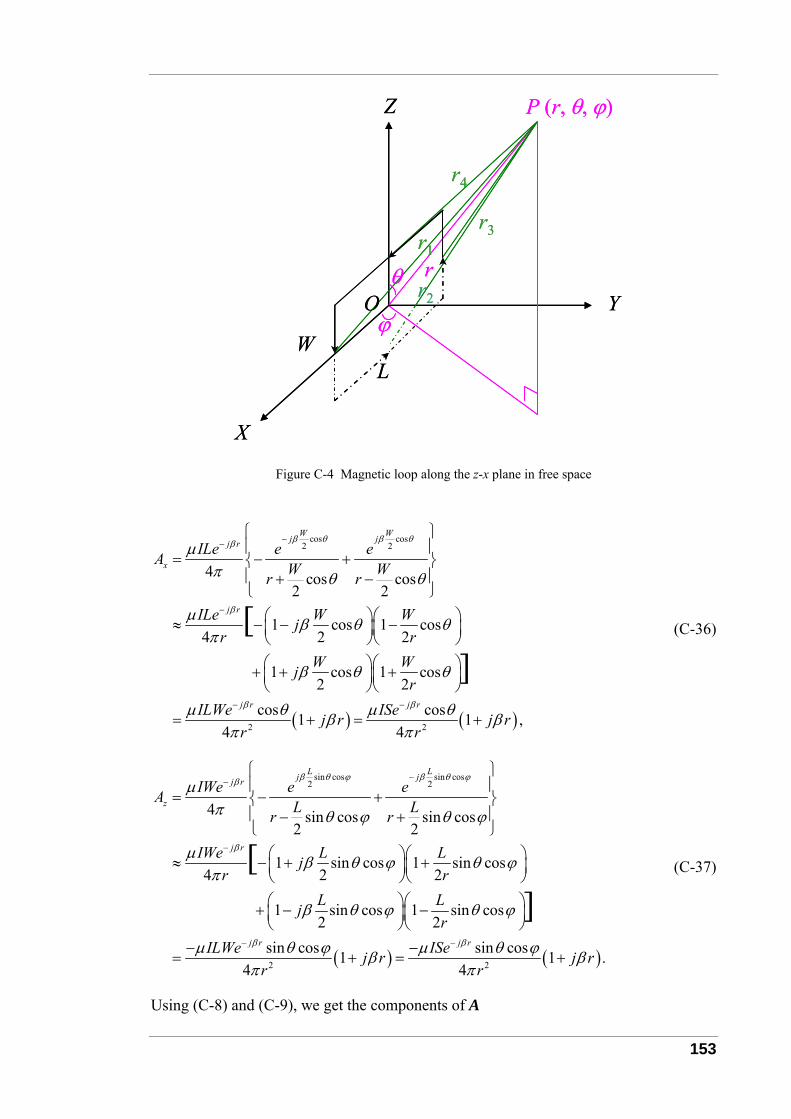
153

Z

Y

P (r, θ, ϕ)

WL

rr1

r2

r3

r4

θ

ϕO

X

Z

Y

P (r, θ, ϕ)

WL

rr1

r2

r3

r4

θ

ϕO

X

Figure C-4 Magnetic loop along the z-x plane in free space

( )

cos cos2 2

2 2

4 cos cos2 2

1 cos 1 cos4 2 2

1 cos 1 cos2 2

cos cos1 14 4

[]

W Wj jj r

x

j r

j r j r

ILe e eA W Wr r

ILe W Wjr r

W Wjr

ILWe ISej r jr r

β θ β θβ

β

β β

μπ θ θ

μ β θ θπ

β θ θ

μ θ μ θβ βπ π

−−

−

− −

⎧ ⎫⎪ ⎪

= − +⎨ ⎬⎪ ⎪+ −⎩ ⎭

⎛ ⎞⎛ ⎞≈ − − −⎜ ⎟⎜ ⎟⎝ ⎠⎝ ⎠⎛ ⎞⎛ ⎞+ + +⎜ ⎟⎜ ⎟⎝ ⎠⎝ ⎠

= + = +( ) ,r

(C-36)

sin cos sin cos2 2

4 sin cos sin cos2 2

1 sin cos 1 sin cos4 2 2

1 sin cos 1 sin cos2 2

[]

L Lj jj r

z

j r

j r

IWe e eA L Lr r

IWe L Ljr r

L Ljr

ILWe

β θ ϕ β θ ϕβ

β

β

μπ θ ϕ θ ϕ

μ β θ ϕ θ ϕπ

β θ ϕ θ ϕ

μ

−−

−

−

⎧ ⎫⎪ ⎪

= − +⎨ ⎬⎪ ⎪− +⎩ ⎭

⎛ ⎞⎛ ⎞≈ − + +⎜ ⎟⎜ ⎟⎝ ⎠⎝ ⎠⎛ ⎞⎛ ⎞+ − −⎜ ⎟⎜ ⎟⎝ ⎠⎝ ⎠

−= ( ) ( )2 2

sin cos sin cos1 1 .4 4

j rISej r j rr r

βθ ϕ μ θ ϕβ βπ π

−−+ = +

(C-37)

Using (C-8) and (C-9), we get the components of A

154

( )

( )

2

2

sin cos cos 0,

cos cos sin 1 cos ,4

sin 1 cos sin .4

r x z

j r

x z

j r

x

A A A

ISeA A A j rr

ISeA A j rr

β

θ

β

ϕ

θ ϕ θ

μθ ϕ θ β ϕπ

μϕ β θ ϕπ

−

−

= + =

= − = +

−= − = +

(C-38)

Using (C-11) and (C-13), we are ready to calculate the magnetic and electric fields,

2 3

2 3

2 3

( sin ) ( )1 1sin sin ,sin 2

( )1 1 1cos sin ,sin 4

( )1 1cos4

j rr

j rr

jr

A A j IS jH er r r

rAA j IS j jH er r r r r

rA A j IS j jH er r r r r

φ βθ

ϕ βθ

θϕ

θ β θ ϕμ θ θ ϕ π β

β βθ ϕμ θ ϕ π β

β βϕμ θ π β

−

−

−

∂⎧ ⎫∂ ⎛ ⎞= − = −⎨ ⎬ ⎜ ⎟∂ ∂ ⎝ ⎠⎩ ⎭

∂⎧ ⎫ ⎛ ⎞∂ −= − = + −⎨ ⎬ ⎜ ⎟∂ ∂ ⎝ ⎠⎩ ⎭

∂ ⎛ ⎞∂ −⎧ ⎫= − = + −⎨ ⎬ ⎜ ⎟∂ ∂⎩ ⎭ ⎝ ⎠;rβ

(C-39)

2

2

( sin ) ( )1 0,sin

( )1 1 1cos ,sin 4

( )1 1cos sin .4

r

j rr

j rr

H HEj r

rHH j IS jE ej r r r r

rH H j IS jE ej r r r r

ϕ θ

ϕ βθ

βθϕ

θωε θ θ ϕ

ωμ βϕωε θ ϕ π

ωμ βθ ϕωε θ π

−

−

∂⎧ ⎫∂= − =⎨ ⎬∂ ∂⎩ ⎭

∂⎧ ⎫∂ − ⎛ ⎞= − = +⎨ ⎬ ⎜ ⎟∂ ∂ ⎝ ⎠⎩ ⎭∂ ∂⎧ ⎫ ⎛ ⎞= − = +⎨ ⎬ ⎜ ⎟∂ ∂ ⎝ ⎠⎩ ⎭

(C-40)

C.2.4 Field of Loop Rotating from any Point

Suppose a small current loop rotates from any point O’ (a, b, c) in OXYZ coordinate

system (See Figure C-5), we make a new coordinate system O’X’Y’Z’ through parallel

offset according to (C-2). At point P, the relationship between (r’, θ’, φ’) and (x, y, z) is

shown in (C-5).

Suppose an is the unit normal vector of the loop plane, and the angle between an and x

(or x’), y (or y’), z (or z’) axis is xα , yα , zα , respectively, then we have (C-4) and

( )cos ,cos ,cosn x y zα α α=a (C-41)

Making projection of loop area into x-y, y-z and z-x plane, we can decompose the

magnetic moment IS into components on three planes, mx, my and mz, respectively.

cos ,cos ,cos .

XY z z

YZ x x

ZX y y

IS m ISIS m ISIS m IS

ααα

= == == =

(C-42)

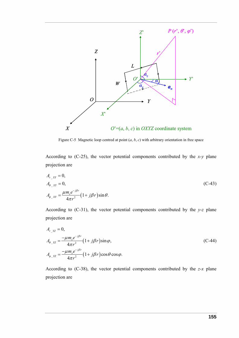
155

X’

Z’

Y’

P (r’, θ’, ϕ’)

W

L

r’

O’αx

αzαy

an

X

Y

Z

O

O’=(a, b, c) in OXYZ coordinate system

X’

Z’

Y’

P (r’, θ’, ϕ’)

W

L

r’

O’αx

αzαy

an

X

Y

Z

O

O’=(a, b, c) in OXYZ coordinate system

Figure C-5 Magnetic loop centred at point (a, b, c) with arbitrary orientation in free space

According to (C-25), the vector potential components contributed by the x-y plane

projection are

( )

_

_

_ 2

0,

0,

1 sin .4

r XY

XY

j rz

XY

A

A

m eA j rr

θ

β

φμ β θ

π

−

=

=

= +

(C-43)

According to (C-31), the vector potential components contributed by the y-z plane

projection are

( )

( )

_

_ 2

_ 2

0,

1 sin ,4

1 cos cos .4

r YZ

j rx

YZ

j rx

YZ

A

m eA j rr

m eA j rr

β

θ

β

ϕ

μ β ϕπ

μ β θ ϕπ

−

−

=

−= +

−= +

(C-44)

According to (C-38), the vector potential components contributed by the z-x plane

projection are

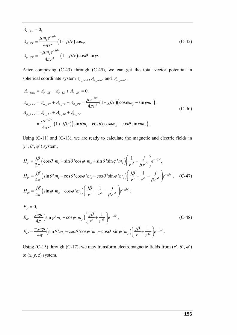
156

( )

( )

_

_ 2

_ 2

0,

1 cos ,4

1 cos sin .4

r ZX

j ry

ZX

j ry

ZX

A

m eA j r

rm e

A j rr

β

θ

β

ϕ

μβ ϕ

πμ

β θ ϕπ

−

−

=

= +

−= +

(C-45)

After composing (C-43) through (C-45), we can get the total vector potential in

spherical coordinate system _r totalA , _ totalAθ and _ totalAϕ .

( )( )

( )( )

_ _ _ _

_ _ _ _ 2

_ _ _ _

2

0,

1 cos sin ,4

1 sin cos cos cos sin .4

r total r XY r YZ r ZX

j r

total XY YZ ZX y x

total XY YZ ZX

j r

z x y

A A A A

eA A A A j r m mr

A A A A

e j r m m mr

β

θ θ θ θ

ϕ ϕ ϕ ϕ

β

μ β ϕ ϕπ

μ β θ θ ϕ θ ϕπ

−

−

= + + =

= + + = + −

= + +

= + − −

(C-46)

Using (C-11) and (C-13), we are ready to calculate the magnetic and electric fields in

(r’, θ’, φ’) system,

( )

( )

( )

'' 2 3

'' 2 3

'' 2 3

1cos ' sin 'cos ' sin 'sin ' ,2 ' '

1sin ' cos 'cos ' cos 'sin ' ,4 ' ' '

1sin ' cos ' ;4 ' ' '

j rr z x y

j rz x y

j rx y

j jH m m m er r

j j jH m m m er r r

j j jH m m er r r

β

βθ

βϕ

β θ θ ϕ θ ϕπ β

β βθ θ ϕ θ ϕπ β

β βϕ ϕπ β

−

−

−

⎛ ⎞= + + −⎜ ⎟

⎝ ⎠⎛ ⎞

= − − + −⎜ ⎟⎝ ⎠

⎛ ⎞= − + −⎜ ⎟

⎝ ⎠

(C-47)

( )

( )

'

'' 2

'' 2

0,1sin ' cos ' ,

4 ' '1sin ' cos 'cos ' cos 'sin ' .

4 ' '

r

j rx y

j rz x y

Ej jE m m e

r rj jE m m m e

r r

βθ

βϕ

ωμ βϕ ϕπωμ βθ θ ϕ θ ϕπ

−

−

=

⎛ ⎞= − +⎜ ⎟⎝ ⎠

− ⎛ ⎞= − − +⎜ ⎟⎝ ⎠

(C-48)

Using (C-15) through (C-17), we may transform electromagnetic fields from (r’, θ’, φ’)

to (x, y, z) system.

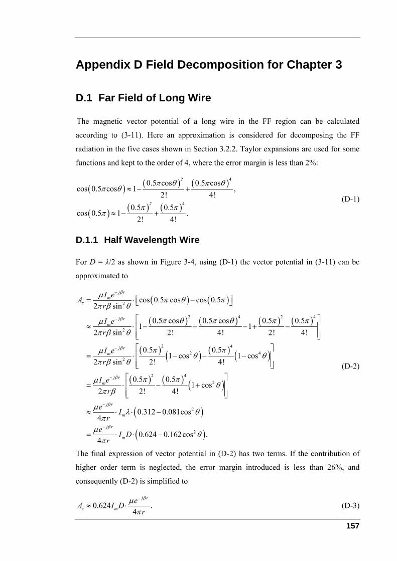
157

Appendix D Field Decomposition for Chapter 3

D.1 Far Field of Long Wire

The magnetic vector potential of a long wire in the FF region can be calculated

according to (3-11). Here an approximation is considered for decomposing the FF

radiation in the five cases shown in Section 3.2.2. Taylor expansions are used for some

functions and kept to the order of 4, where the error margin is less than 2%:

( ) ( ) ( )

( ) ( ) ( )

4

4

0.5 cos 0.5 coscos 0.5 cos 1 ,

2! 4!0.5 0.5

cos 0.5 1 .2! 4!

2

2

π θ π θπ θ

π ππ

≈ − +

≈ − +

(D-1)

D.1.1 Half Wavelength Wire

For D = λ/2 as shown in Figure 3-4, using (D-1) the vector potential in (3-11) can be

approximated to

( ) ( )

( ) ( ) ( ) ( )

( ) ( ) ( ) ( )

( ) ( )

2

2 4 2 4

2

2 42 4

2

2 4

cos 0.5 cos cos 0.52 sin

0.5 cos 0.5 cos 0.5 0.51 1

2 sin 2! 4! 2! 4!

0.5 0.51 cos 1 cos

2 sin 2! 4!

0.5 0.51

2 2! 4!

j rm

z

j rm

j rm

j rm

I eAr

I er

I er

I er

β

β

β

β

μ π θ ππ β θ

π θ π θ π πμπ β θ

π πμ θ θπ β θ

π πμπ β

−

−

−

−

= ⋅ −⎡ ⎤⎣ ⎦

⎡ ⎤≈ ⋅ − + − + −⎢ ⎥

⎢ ⎥⎣ ⎦⎡ ⎤

= ⋅ − − −⎢ ⎥⎢ ⎥⎣ ⎦

= ⋅ − ( )

( )

( )

2

2

2

cos

0.312 0.081cos4

0.624 0.162cos .4

j r

m

j r

m

e Ir

e I Dr

β

β

θ

μ λ θπ

μ θπ

−

−

⎡ ⎤+⎢ ⎥

⎢ ⎥⎣ ⎦

≈ ⋅ ⋅ −

= ⋅ ⋅ −

(D-2)

The final expression of vector potential in (D-2) has two terms. If the contribution of

higher order term is neglected, the error margin introduced is less than 26%, and

consequently (D-2) is simplified to

0.624 .4

j r

z meA I D

r

βμπ

−

≈ ⋅ (D-3)

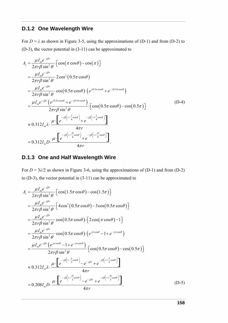
158

D.1.2 One Wavelength Wire

For D = λ as shown in Figure 3-5, using the approximations of (D-1) and from (D-2) to

(D-3), the vector potential in (3-11) can be approximated to

( ) ( )

( )

( ) ( )

( ) ( ) ( )

2

22

0.5 cos 0.5 cos2

0.5 cos 0.5 cos

2

cos cos cos2 sin

2cos 0.5 cos2 sin

cos 0.5 cos2 sin

cos 0.5 cos cos 0.52 sin

0.312[

j rm

z

j rm

j rj jm

j r j jm

m

I eArI erI e e er

I e e er

I

β

β

βπ θ π θ

β π θ π θ

μ π θ ππ β θμ π θπ β θμ π θπ β θ

μπ θ π

π β θ

μλ

−

−

−−

− −

= ⋅ −⎡ ⎤⎣ ⎦

= ⋅

= ⋅ ⋅ +

+= ⋅ −⎡ ⎤⎣ ⎦

⋅≈ ⋅

cos cos4 4

cos cos4 4

4

0.312 .4

]

[ ]

j r j r

D Dj r j r

m

e er

e eI D

r

λ λβ θ β θ

β θ β θ

π

μπ

⎛ ⎞ ⎛ ⎞− − − +⎜ ⎟ ⎜ ⎟⎝ ⎠ ⎝ ⎠

⎛ ⎞ ⎛ ⎞− − − +⎜ ⎟ ⎜ ⎟⎝ ⎠ ⎝ ⎠

+

⋅ += ⋅

(D-4)

D.1.3 One and Half Wavelength Wire

For D = 3λ/2 as shown in Figure 3-6, using the approximations of (D-1) and from (D-2)

to (D-3), the vector potential in (3-11) can be approximated to

( ) ( )

( ) ( )

( ) ( )

( ) ( )

2

32

2

cos cos2

cos 1.5 cos cos 1.52 sin

4cos 0.5 cos 3cos 0.5 cos2 sin

cos 0.5 cos 2cos cos 12 sin

cos 0.5 cos 12 sin

j rm

z

j rm

j rm

j rj jm

j r jm

I eArI erI erI e e er

I e e

β

β

β

βπ θ π θ

β π

μ π θ ππ β θμ π θ π θπ β θμ π θ π θπ β θμ π θπ β θ

μ

−

−

−

−−

−

= ⋅ −⎡ ⎤⎣ ⎦

⎡ ⎤= ⋅ −⎣ ⎦

= ⋅ ⋅ −⎡ ⎤⎣ ⎦

= ⋅ ⋅ − +

=( ) ( ) ( )

cos cos

2

cos cos2 2

cos cos3 3

1cos 0.5 cos cos 0.5

2 sin

0.3124

0.208 .4

[ ]

[ ]

j

j r j rj r

m

D Dj r j rj r

m

er

e e eI

r

e e eI D

r

θ π θ

λ λβ θ β θβ

β θ β θβ

π θ ππ β θ

μλ

π

μπ

−

⎛ ⎞ ⎛ ⎞− − − +⎜ ⎟ ⎜ ⎟−⎝ ⎠ ⎝ ⎠

⎛ ⎞ ⎛ ⎞− − − +⎜ ⎟ ⎜ ⎟−⎝ ⎠ ⎝ ⎠

− +⋅ −⎡ ⎤⎣ ⎦

⋅ − +≈ ⋅

⋅ − += ⋅ (D-5)

159

D.1.4 Double Wavelength Wire

For D = 2λ as shown in Figure 3-7, using the approximations of (D-1) and from (D-2) to

(D-3), the vector potential in (3-11) can be approximated to

( ) ( )

( ) ( ) ( )

( )

( ) ( )

2

2

1.5 cos 0.5 cos 0.5 cos 1.5 cos

2

cos 2 cos cos 22 sin

4sin 0.5 cos cos 0.5 cos sin cos2 sin

2 sin cos 0.5 cos cos 0.5

0.312[

j rm

z

j rm

j r j j j jm

m

I eArI er

I e e e e er

eI

β

β

β π θ π θ π θ π θ

μ π θ ππ β θμ π θ π θ π θπ β θ

μ

π β θ

π θ π

μλ

−

−

− − −

= ⋅ −⎡ ⎤⎣ ⎦

= ⋅ − ⋅ ⋅⎡ ⎤⎣ ⎦

− − += ⋅

−⎡ ⎤⎣ ⎦

≈ ⋅

3 3cos cos cos cos4 4 4 4

3 3cos cos cos cos8 8 8 8

4

0.156 .4

]

[ ]

j r j r j r j r

D D D Dj r j r j r j r

m

e e er

e e e eI D

r

λ λ λ λβ θ β θ β θ β θ

β θ β θ β θ β θ

π

μπ

⎛ ⎞ ⎛ ⎞ ⎛ ⎞ ⎛ ⎞− − − − − + − +⎜ ⎟ ⎜ ⎟ ⎜ ⎟ ⎜ ⎟⎝ ⎠ ⎝ ⎠ ⎝ ⎠ ⎝ ⎠

⎛ ⎞ ⎛ ⎞ ⎛ ⎞ ⎛ ⎞− − − − − + − +⎜ ⎟ ⎜ ⎟ ⎜ ⎟ ⎜ ⎟⎝ ⎠ ⎝ ⎠ ⎝ ⎠ ⎝ ⎠

− − +

− − += ⋅

(D-6)

D.1.5 Two and Half Wavelength Wire

For D = 5λ/2 as shown in Figure 3-8, using the approximations of (D-1) and from (D-2)

to (D-3), the vector potential in (3-11) can be approximated to

( ) ( )

( ) ( ) ( ) ( )

( )

( ) ( )

2

2

2

22 cos 2 cos 0.5 cos 0.5 cos cos

cos 2.5 cos cos 2.52 sin

cos 2 cos cos 0.5 cos sin 2 cos sin 0.5 cos2 sin

cos 0.5 cos2 sin

1 2

j rm

z

j rm

j rm

j j j j j

I eArI erI er

e e e e e e

β

β

β

π θ π θ π θ π θ π θ

μ π θ ππ β θμ π θ π θ π θ π θπ β θμ π θπ β θ

−

−

−

− − −

= ⋅ −⎡ ⎤⎣ ⎦

= ⋅ ⋅ − ⋅⎡ ⎤⎣ ⎦

= ⋅ ⋅

+ + − ⋅ +( )( )

( ) ( )

( ) ( )

cos

2 cos cos cos 2 cos

2

cos coscos cos2 2

2 c5

12 sin

cos 0.5 cos cos 0.5

0.3124

0.125

[ ]

[

j

j r j j j jm

j r j rj r j rj r

m

Dj r

m

I e e e e er

e e e e eI

r

eI D

π θ

β π θ π θ π θ π θ

λ λβ θ β θβ λ θ β λ θβ

β

μ

π β θ

π θ π

μλ

π

μ

− − −

⎛ ⎞ ⎛ ⎞− − − +⎜ ⎟ ⎜ ⎟− − − +−⎝ ⎠ ⎝ ⎠

− −

⎡ ⎤⎢ ⎥⎣ ⎦

− + − += ⋅

−⎡ ⎤⎣ ⎦

− + − +≈ ⋅

= ⋅

2os cos cos cos5 5 5

.4

]D D Dj r j r j rj re e e er

θ β θ β θ β θβ

π

⎛ ⎞ ⎛ ⎞ ⎛ ⎞ ⎛ ⎞− − − + − +⎜ ⎟ ⎜ ⎟ ⎜ ⎟ ⎜ ⎟−⎝ ⎠ ⎝ ⎠ ⎝ ⎠ ⎝ ⎠− + − + (D-7)

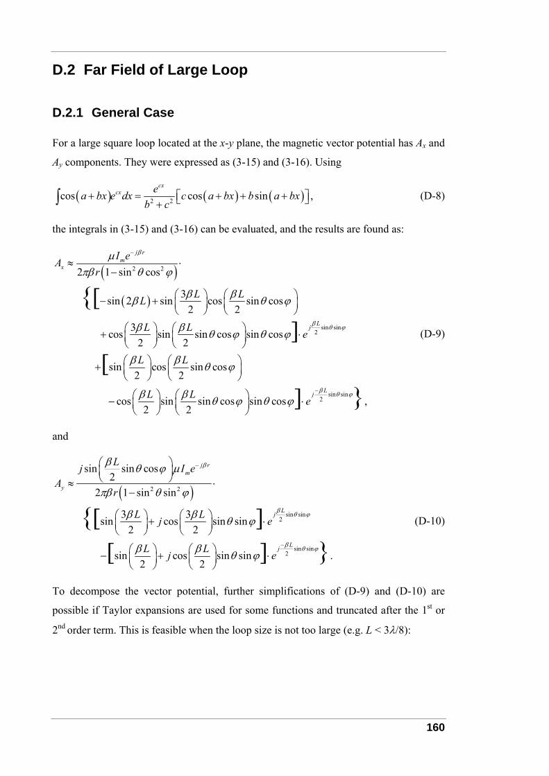
160

D.2 Far Field of Large Loop

D.2.1 General Case

For a large square loop located at the x-y plane, the magnetic vector potential has Ax and

Ay components. They were expressed as (3-15) and (3-16). Using

( ) ( ) ( )2 2cos cos sin ,cx

cx ea bx e dx c a bx b a bxb c

+ = + + +⎡ ⎤⎣ ⎦+∫ (D-8)

the integrals in (3-15) and (3-16) can be evaluated, and the results are found as:

( )

( )

2 2

sin sin2

2 1 sin cos

3 sin 2 sin cos sin cos2 2

3 cos sin sin cos sin cos2 2

sin cos sin cos2 2

[]

[

j rm

x

Lj

I eAr

L LL

L L e

L L

β

β θ ϕ

μπβ θ ϕ

β ββ θ ϕ

β β θ ϕ θ ϕ

β β θ ϕ

−

≈ ⋅−

⎛ ⎞ ⎛ ⎞− + ⎜ ⎟ ⎜ ⎟⎝ ⎠ ⎝ ⎠

⎛ ⎞ ⎛ ⎞+ ⋅⎜ ⎟ ⎜ ⎟⎝ ⎠ ⎝ ⎠⎛ ⎞ ⎛ ⎞+ ⎜ ⎟ ⎜⎝ ⎠ ⎝

sin sin2 cos sin sin cos sin cos ,

2 2] LjL L e

β θ ϕβ β θ ϕ θ ϕ−

⎟⎠

⎛ ⎞ ⎛ ⎞− ⋅⎜ ⎟ ⎜ ⎟⎝ ⎠ ⎝ ⎠

(D-9)

and

( )2 2

sin sin2

sin sin2

sin sin cos2

2 1 sin sin

3 3 sin cos sin sin2 2

sin cos sin sin .2 2

[ ][ ]

j rm

y

Lj

Lj

Lj I eA

r

L Lj e

L Lj e

β

β θ ϕ

β θ ϕ

β θ ϕ μ

πβ θ ϕ

β β θ ϕ

β β θ ϕ

−

−

⎛ ⎞⎜ ⎟⎝ ⎠≈ ⋅

−

⎛ ⎞ ⎛ ⎞+ ⋅⎜ ⎟ ⎜ ⎟⎝ ⎠ ⎝ ⎠

⎛ ⎞ ⎛ ⎞− + ⋅⎜ ⎟ ⎜ ⎟⎝ ⎠ ⎝ ⎠

(D-10)

To decompose the vector potential, further simplifications of (D-9) and (D-10) are

possible if Taylor expansions are used for some functions and truncated after the 1st or

2nd order term. This is feasible when the loop size is not too large (e.g. L < 3λ/8):

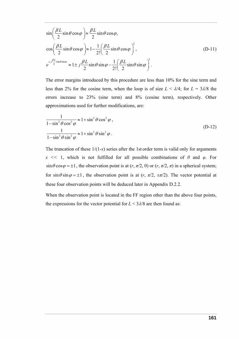
161

2

2sin sin

2

sin sin cos sin cos ,2 2

1cos sin cos 1 sin cos ,2 2! 2

11 sin sin sin sin .2 2! 2

Lj

L L

L L

L Le jβ θ ϕ

β βθ ϕ θ ϕ

β βθ ϕ θ ϕ

β βθ ϕ θ ϕ±

⎛ ⎞ ≈⎜ ⎟⎝ ⎠

⎛ ⎞ ⎛ ⎞≈ −⎜ ⎟ ⎜ ⎟⎝ ⎠ ⎝ ⎠

⎛ ⎞≈ ± − ⎜ ⎟⎝ ⎠

(D-11)

The error margins introduced by this procedure are less than 10% for the sine term and

less than 2% for the cosine term, when the loop is of size L < λ/4; for L = 3λ/8 the

errors increase to 23% (sine term) and 8% (cosine term), respectively. Other

approximations used for further modifications, are:

2 22 2

2 22 2

1 1 sin cos ,1 sin cos

1 1 sin sin .1 sin sin

θ ϕθ ϕ

θ ϕθ ϕ

≈ +−

≈ +−

(D-12)

The truncation of these 1/(1-x) series after the 1st order term is valid only for arguments

x << 1, which is not fulfilled for all possible combinations of θ and φ. For

sin cos 1θ ϕ = ± , the observation point is at (r, π/2, 0) or (r, π/2, π) in a spherical system;

for sin sin 1θ ϕ = ± , the observation point is at (r, π/2, ±π/2). The vector potential at

these four observation points will be deduced later in Appendix D.2.2.

When the observation point is located in the FF region other than the above four points,

the expressions for the vector potential for L < 3λ/8 are then found as:

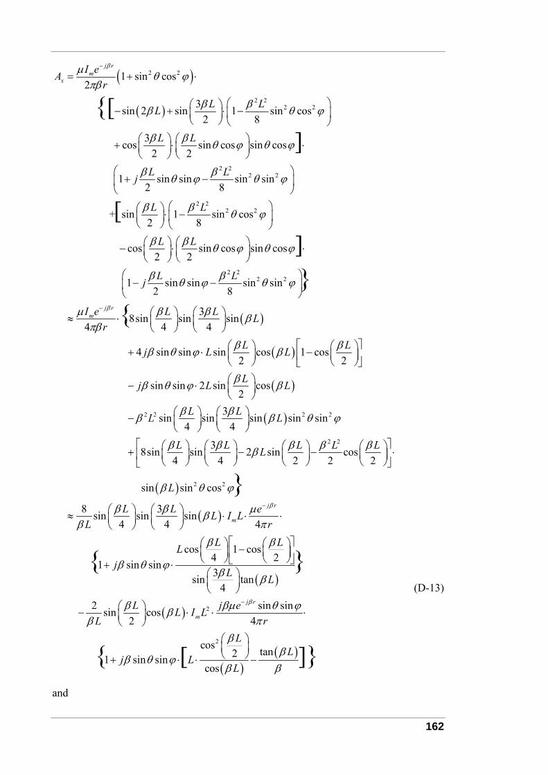
162

( )

( )

2 2

2 22 2

2 22 2

1 sin cos2

3sin 2 sin 1 sin cos2 8

3 cos sin cos sin cos2 2

1 sin sin sin sin2 8

[]

j rm

xI eA

r

L LL

L L

L Lj

βμ θ ϕπβ

β ββ θ ϕ

β β θ ϕ θ ϕ

β βθ ϕ θ ϕ

−

= + ⋅

⎛ ⎞⎛ ⎞− + ⋅ −⎜ ⎟⎜ ⎟⎝ ⎠ ⎝ ⎠

⎛ ⎞ ⎛ ⎞+ ⋅ ⋅⎜ ⎟ ⎜ ⎟⎝ ⎠ ⎝ ⎠

⎛ ⎞+ −⎜ ⎟

⎝ ⎠

( )

2 22 2

2 22 2

+ sin 1 sin cos2 8

cos sin cos sin cos2 2

1 sin sin sin sin2 8

38sin sin sin4 4 4

[]

j rm

L L

L L

L Lj

I e L L Lr

β

β β θ ϕ

β β θ ϕ θ ϕ

β βθ ϕ θ ϕ

μ β β βπβ

−

⎛ ⎞⎛ ⎞ ⋅ −⎜ ⎟⎜ ⎟⎝ ⎠ ⎝ ⎠⎛ ⎞ ⎛ ⎞− ⋅ ⋅⎜ ⎟ ⎜ ⎟⎝ ⎠ ⎝ ⎠

⎛ ⎞− −⎜ ⎟

⎝ ⎠

⎛ ⎞ ⎛ ⎞≈ ⋅ ⎜ ⎟ ⎜ ⎟⎝ ⎠ ⎝ ⎠

( )

( )

( )2 2 2 2

4 sin sin sin cos 1 cos2 2

sin sin 2 sin cos2

3 sin sin sin sin sin4 4

L Lj L L

Lj L L

L LL L

β ββ θ ϕ β

ββ θ ϕ β

β ββ β θ ϕ

⎡ ⎤⎛ ⎞ ⎛ ⎞+ ⋅ −⎜ ⎟ ⎜ ⎟⎢ ⎥⎝ ⎠ ⎝ ⎠⎣ ⎦⎛ ⎞− ⋅ ⎜ ⎟⎝ ⎠

⎛ ⎞ ⎛ ⎞− ⎜ ⎟ ⎜ ⎟⎝ ⎠ ⎝ ⎠

( )

( )

2 2

2 2

3 8sin sin 2 sin cos4 4 2 2 2

sin sin cos

8 3sin sin sin4 4 4

cos 1 cos41 sin sin

j r

m

L L L L LL

L

L L eL I LL r

L LLj

β

β β β β ββ

β θ ϕ

β β μββ π

β β

β θ ϕ

−

⎡ ⎤⎛ ⎞ ⎛ ⎞ ⎛ ⎞ ⎛ ⎞+ − − ⋅⎜ ⎟ ⎜ ⎟ ⎜ ⎟ ⎜ ⎟⎢ ⎥⎝ ⎠ ⎝ ⎠ ⎝ ⎠ ⎝ ⎠⎣ ⎦

⎛ ⎞ ⎛ ⎞≈ ⋅ ⋅ ⋅⎜ ⎟ ⎜ ⎟⎝ ⎠ ⎝ ⎠

⎛ ⎞ −⎜ ⎟⎝ ⎠+ ⋅

( )

( )

( )( )

2

2

23sin tan

42 sin sin sin cos

2 4

cos tan21 sin sincos

[ ]

j r

m

L L

L j eL I LL r

LL

j LL

β

β β

β βμ θ ϕββ π

ββ

β θ ϕβ β

−

⎡ ⎤⎛ ⎞⎜ ⎟⎢ ⎥⎝ ⎠⎣ ⎦

⎛ ⎞⎜ ⎟⎝ ⎠

⎛ ⎞− ⋅ ⋅ ⋅⎜ ⎟⎝ ⎠

⎛ ⎞⎜ ⎟⎝ ⎠+ ⋅ ⋅ −

(D-13)

and

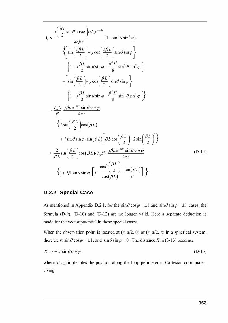
163

( )2 2

2 22 2

sin cos2 1 sin sin

2

3 3sin cos sin sin2 2

1 sin sin sin sin2 8

sin cos sin sin2 2

j rm

y

Lj I eA

r

L Lj

L Lj

L Lj

ββ θ ϕ μθ ϕ

πβ

β β θ ϕ

β βθ ϕ θ ϕ

β β θ ϕ

−⎛ ⎞⎜ ⎟⎝ ⎠≈ + ⋅

⎡ ⎤⎛ ⎞ ⎛ ⎞+ ⋅⎜ ⎟ ⎜ ⎟⎢ ⎥⎝ ⎠ ⎝ ⎠⎣ ⎦⎛ ⎞+ −⎜ ⎟

⎝ ⎠⎡ ⎤⎛ ⎞ ⎛ ⎞− + ⋅⎜ ⎟ ⎜ ⎟⎢ ⎥⎝ ⎠ ⎝ ⎠⎣ ⎦

( )

( )

( )

2 22 2

2

1 sin sin sin sin2 8

sin cos4

2sin cos2

sin sin sin cos 2sin2 2

2 sin cossin cos2 4

j rm

j r

m

L Lj

I L j er

L L

L Lj L L

L j eL I LL r

β

β

β βθ ϕ θ ϕ

βμ θ ϕβ π

β β

β βθ ϕ β β

β βμ θ ϕββ π

−

−

⎛ ⎞− −⎜ ⎟

⎝ ⎠

≈ ⋅ ⋅

⎛ ⎞⎜ ⎟⎝ ⎠

⎡ ⎤⎛ ⎞ ⎛ ⎞+ ⋅ −⎜ ⎟ ⎜ ⎟⎢ ⎥⎝ ⎠ ⎝ ⎠⎣ ⎦

⎛ ⎞≈ ⋅ ⋅ ⋅⎜ ⎟⎝ ⎠

( )( )

2cos tan21 sin sin .cos

[ ] L

Lj L

L

ββ

β θ ϕβ β

⎛ ⎞⎜ ⎟⎝ ⎠+ ⋅ ⋅ −

(D-14)

D.2.2 Special Case

As mentioned in Appendix D.2.1, for the sin cos 1θ ϕ = ± and sin sin 1θ ϕ = ± cases, the

formula (D-9), (D-10) and (D-12) are no longer valid. Here a separate deduction is

made for the vector potential in these special cases.

When the observation point is located at (r, π/2, 0) or (r, π/2, π) in a spherical system,

there exist sin cos 1θ ϕ = ± , and sin sin 0θ ϕ = . The distance R in (3-13) becomes

'sin cos ,R r x θ ϕ≈ − (D-15)

where x’ again denotes the position along the loop perimeter in Cartesian coordinates.

Using

164

( ) ( ) ( ) ( )( ) ( )

( )2

cos cos cos sin

cos 2 cos sin 2 sin2 2

,2 4

jbx

jaj a bx

a bx e dx a bx bx j bx dx

a bx a a bx aj dx

e jx eb

−+

+ = + ⋅ +⎡ ⎤⎣ ⎦

+ + + −⎡ ⎤= +⎢ ⎥

⎣ ⎦

= ⋅ − ⋅

∫ ∫

∫ (D-16)

the magnetic vector potential components in (3-15) and (3-16) can be evaluated, and the

results are found as:

( ) ( )

( )

( ) ( )

0 / 2

/ 2 0

/ 2

/ 2

2

cos 2 cos 24

cos

2sin sin sin2 4

1cos cos sin4 2 2 2 2

8 sin4

[]

j r Lj x j xx m L

L j x

L

j r

m

eA I x L e dx x L e dxr

x e dx

L eL L I LL r

L L L L

LL

ββ β

β

β

μ β β β βπ

β

β μβ ββ π

β β β β

ββ

−

−

−

−

≈ ⋅ − + − −

+

⎡ ⎤⎛ ⎞= + ⋅ ⋅ ⋅⎜ ⎟⎢ ⎥⎝ ⎠⎣ ⎦⎡ ⎤⎛ ⎞ ⎛ ⎞ ⎛ ⎞= ⋅ + ⋅ ⋅⎜ ⎟ ⎜ ⎟ ⎜ ⎟⎢ ⎥⎝ ⎠ ⎝ ⎠ ⎝ ⎠⎣ ⎦

⎛⎜⎝

∫ ∫

∫

( )sin ,4

j r

meL I L

r

βμβπ

−⎞ ⋅ ⋅⎟⎠

(D-17)

and

( ) ( )

( )

/ 2 / 22 2

/ 2 / 2

2

cos cos4

4 sin cos .4 2

[ ]L Lj r L Lj j

y m L L

j r

m

eA I y L e dy y L e dyr

e j LI Lr

β ββ

β

μ β β β βπ

μ β βπ β

−−

− −

−

≈ ⋅ − + + +

⎛ ⎞= ⋅ ⎜ ⎟⎝ ⎠

∫ ∫ (D-18)

When the loop size is not too large (e.g. L < 3λ/8), further simplifications of (D-17) and

(D-18) are possible if the following Taylor expansions are used and truncated after the

1st order term:

sin ,2 2

cos 1.4

L L

L

β β

β

⎛ ⎞ ≈⎜ ⎟⎝ ⎠

⎛ ⎞ ≈⎜ ⎟⎝ ⎠

(D-19)

The error margins introduced by this procedure are less than 23% for the sine term and

less than 17% for the cosine term when the loop is of size L < 3λ/8.

When the observation point is located at (r, π/2, 0) or (r, π/2, π) in a spherical system,

the expressions for the vector potential for L < 3λ/8 are then found as:

165

( )

( )

1 8sin cos sin sin sin2 2 2 2 4 4

8 3sin sin sin ,4 4 4

j r

x m

j r

m

L L L L eA L I LL r

L L eL I LL r

β

β

β β β β μββ π

β β μββ π

−

−

⎡ ⎤⎛ ⎞ ⎛ ⎞ ⎛ ⎞ ⎛ ⎞≈ ⋅ + ⋅ ⋅ ⋅ ⋅⎜ ⎟ ⎜ ⎟ ⎜ ⎟ ⎜ ⎟⎢ ⎥⎝ ⎠ ⎝ ⎠ ⎝ ⎠ ⎝ ⎠⎣ ⎦

⎛ ⎞ ⎛ ⎞= ⋅ ⋅⎜ ⎟ ⎜ ⎟⎝ ⎠ ⎝ ⎠

(D-20)

( ) 22 sin cos .2 4

j r

y mL j eA L I L

L r

ββ βμββ π

−⎛ ⎞≈ ⋅ ⋅⎜ ⎟⎝ ⎠

(D-21)

For this sin cos 1θ ϕ = ± case, both (D-20) and (D-21) conform to the vector potential

formula (D-13) and (D-14) in general case, respectively.

When the observation point is located at (r, π/2, ±π/2) in a spherical system, there exist

sin sin 1θ ϕ = ± , and sin cos 0θ ϕ = . The distance R in (3-13) becomes

'sin sin ,R r y θ ϕ≈ − (D-22)

where y’ again denotes the position along the loop perimeter in Cartesian coordinates.

The magnetic vector potential components in (3-15) and (3-16) can be evaluated, and

the results are found as:

( ) ( )

( )

( )

( )

0 / 22 2

/ 2 0

/ 22

/ 2

cos 2 cos 24

cos

8 3sin sin sin cos4 4 4 2

8 sin cos sin c2 4 4

[]

L Lj r Lj j

x m L

LL j

Lj r

m

j r

m

eA I x L e dx x L e dxr

x e dx

L L e LL I LL r

L L j eL I LL r

β ββ

β

β

β

μ β β β βπ

β

β β μ βββ π

β β μββ π

−

−

−

−

−

−

≈ ⋅ − + − −

+

⎛ ⎞ ⎛ ⎞ ⎛ ⎞= ⋅ ⋅ ⋅⎜ ⎟ ⎜ ⎟ ⎜ ⎟⎝ ⎠ ⎝ ⎠ ⎝ ⎠

⎛ ⎞ ⎛ ⎞− ⋅ ⋅ ⋅⎜ ⎟ ⎜ ⎟⎝ ⎠ ⎝ ⎠

∫ ∫

∫

3os ,4

Lβ⎛ ⎞⎜ ⎟⎝ ⎠

(D-23)

and

( ) ( )/ 2 / 2

/ 2 / 2cos cos 0.

4[ ]j r L Lj y j y

y m L L

eA I y L e dy y L e dyr

ββ βμ β β β β

π

−

− −≈ ⋅ − + + + =∫ ∫ (D-24)

When the loop size is not too large (e.g. L < 3λ/8), the following truncated Taylor

expansion introduces less than 6% error margin:

sin .4 4L Lβ β⎛ ⎞ ≈⎜ ⎟

⎝ ⎠ (D-25)

When the observation point is located at (r, π/2, ±π/2) in a spherical system, using

(D-25) in (D-23), Ax for L < 3λ/8 is then found as:

166

( )

( ) 2

8 3sin sin sin cos4 4 4 2

2 3 sin cos cos .2 4 4

j r

x m

j r

m

L L e LA L I LL r

L j e LL I LL r

β

β

β β μ βββ π

β βμ βββ π

−

−

⎛ ⎞ ⎛ ⎞ ⎛ ⎞≈ ⋅ ⋅ ⋅⎜ ⎟ ⎜ ⎟ ⎜ ⎟⎝ ⎠ ⎝ ⎠ ⎝ ⎠

⎛ ⎞ ⎛ ⎞− ⋅ ⋅ ⋅⎜ ⎟ ⎜ ⎟⎝ ⎠ ⎝ ⎠

(D-26)

For this sin sin 1θ ϕ = ± case, (D-24) matches with the Ay formula (D-14) in general

case. With respect to Ax, (D-26) basically conforms to (D-13), except for not exactly

obtaining the 1 sin sinj yβ θ ϕ+ item in (D-13).

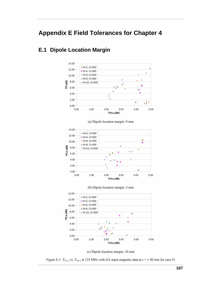
167

Appendix E Field Tolerances for Chapter 4

E.1 Dipole Location Margin

0.00

2.00

4.00

6.00

8.00

10.00

12.00

14.00

0.00 1.00 2.00 3.00 4.00 5.00Tnf,a (dB)

Tff (

dB)

N=2, G=500N=4, G=500N=6, G=500N=8, G=500N=10, G=500

(a) Dipole location margin: 0 mm

0.00

2.00

4.00

6.00

8.00

10.00

12.00

14.00

0.00 1.00 2.00 3.00 4.00 5.00Tnf,a (dB)

Tff,a

(dB

)

N=2, G=500N=4, G=500N=6, G=500N=8, G=500N=10, G=500

(b) Dipole location margin: 5 mm

0.00

2.00

4.00

6.00

8.00

10.00

12.00

14.00

0.00 1.00 2.00 3.00 4.00 5.00Tnf,a (dB)

Tff,a

(dB

)

N=2, G=500N=4, G=500N=6, G=500N=8, G=500N=10, G=500

(c) Dipole location margin: 10 mm

Figure E-1 TFF,a vs. TNF,a at 125 MHz with GA input magnetic data at z = ± 40 mm for case #1

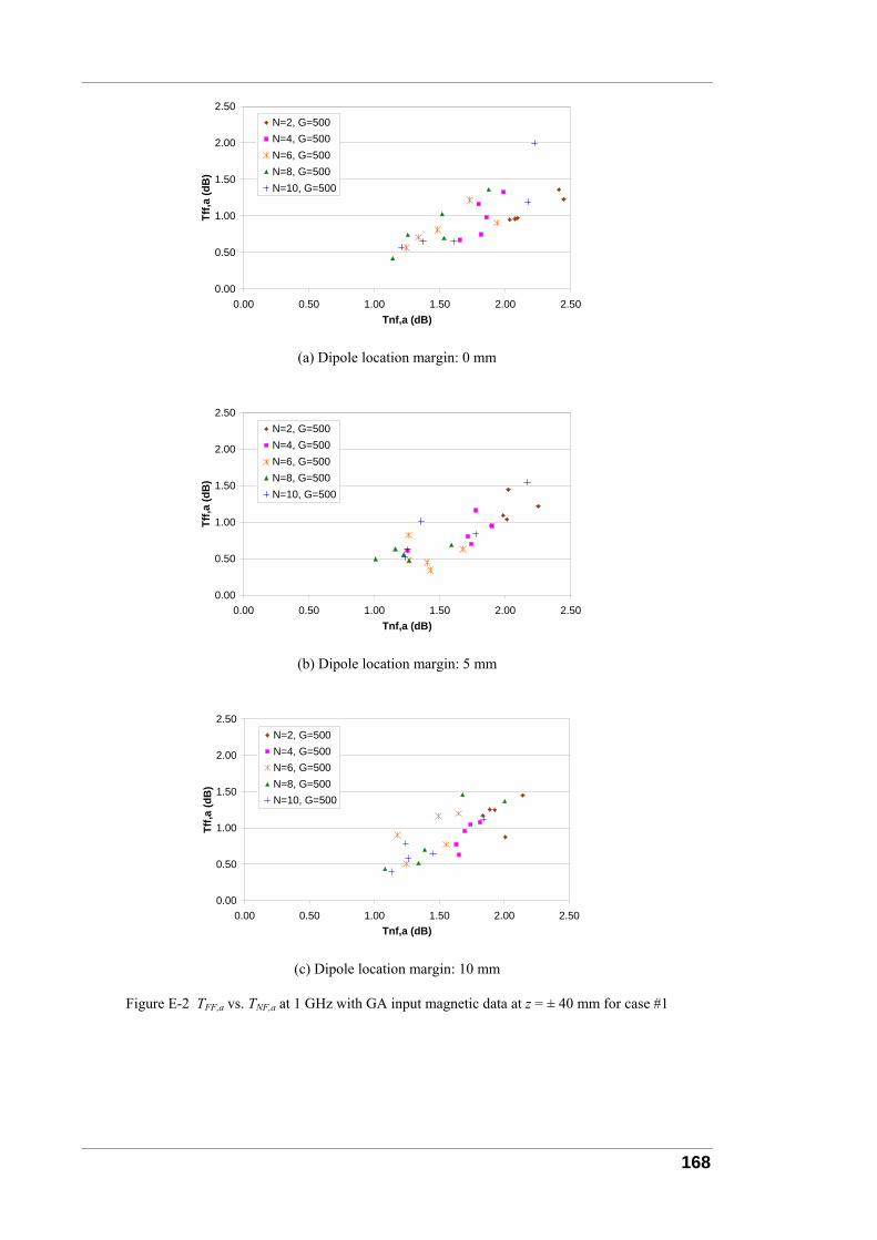
168

0.00

0.50

1.00

1.50

2.00

2.50

0.00 0.50 1.00 1.50 2.00 2.50Tnf,a (dB)

Tff,a

(dB

)

N=2, G=500N=4, G=500N=6, G=500N=8, G=500N=10, G=500

(a) Dipole location margin: 0 mm

0.00

0.50

1.00

1.50

2.00

2.50

0.00 0.50 1.00 1.50 2.00 2.50Tnf,a (dB)

Tff,a

(dB

)

N=2, G=500N=4, G=500N=6, G=500N=8, G=500N=10, G=500

(b) Dipole location margin: 5 mm

0.00

0.50

1.00

1.50

2.00

2.50

0.00 0.50 1.00 1.50 2.00 2.50Tnf,a (dB)

Tff,a

(dB

)

N=2, G=500N=4, G=500N=6, G=500N=8, G=500N=10, G=500

(c) Dipole location margin: 10 mm

Figure E-2 TFF,a vs. TNF,a at 1 GHz with GA input magnetic data at z = ± 40 mm for case #1

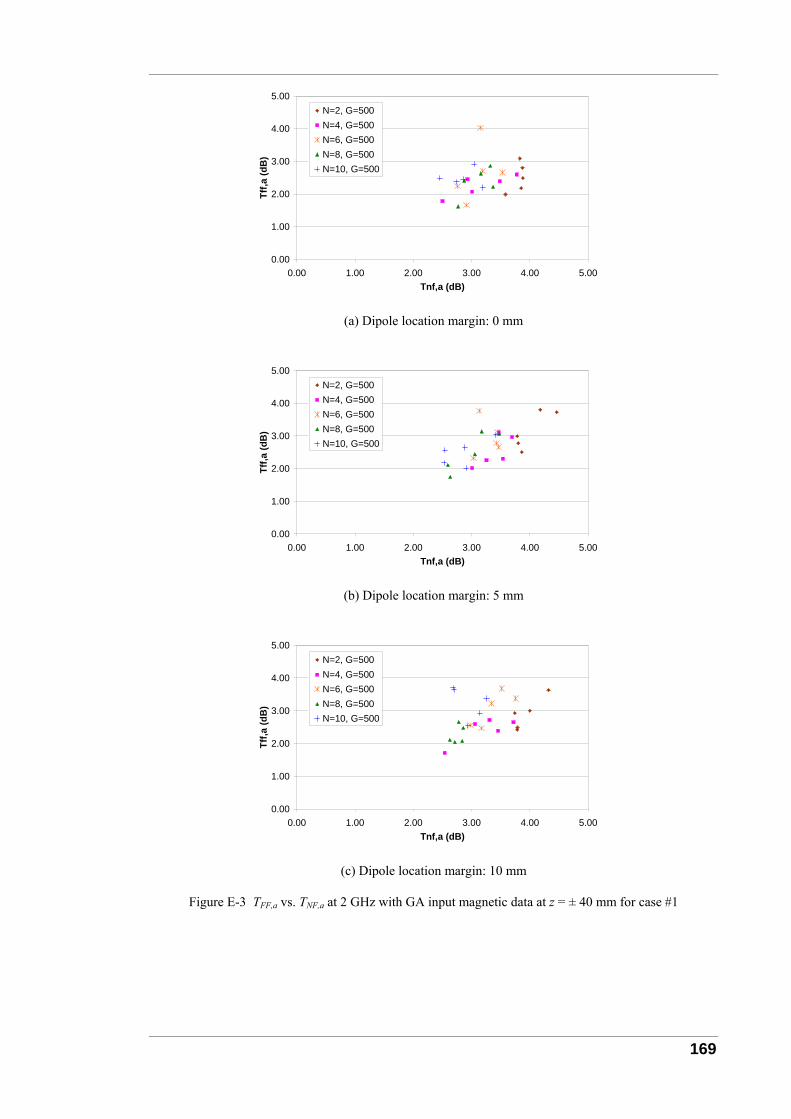
169

0.00

1.00

2.00

3.00

4.00

5.00

0.00 1.00 2.00 3.00 4.00 5.00Tnf,a (dB)

Tff,a

(dB

)

N=2, G=500N=4, G=500N=6, G=500N=8, G=500N=10, G=500

(a) Dipole location margin: 0 mm

0.00

1.00

2.00

3.00

4.00

5.00

0.00 1.00 2.00 3.00 4.00 5.00Tnf,a (dB)

Tff,a

(dB

)

N=2, G=500N=4, G=500N=6, G=500N=8, G=500N=10, G=500

(b) Dipole location margin: 5 mm

0.00

1.00

2.00

3.00

4.00

5.00

0.00 1.00 2.00 3.00 4.00 5.00Tnf,a (dB)

Tff,a

(dB

)

N=2, G=500N=4, G=500N=6, G=500N=8, G=500N=10, G=500

(c) Dipole location margin: 10 mm

Figure E-3 TFF,a vs. TNF,a at 2 GHz with GA input magnetic data at z = ± 40 mm for case #1

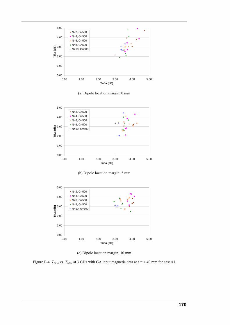
170

0.00

1.00

2.00

3.00

4.00

5.00

0.00 1.00 2.00 3.00 4.00 5.00Tnf,a (dB)

Tff,a

(dB

)

N=2, G=500N=4, G=500N=6, G=500N=8, G=500N=10, G=500

(a) Dipole location margin: 0 mm

0.00

1.00

2.00

3.00

4.00

5.00

0.00 1.00 2.00 3.00 4.00 5.00Tnf,a (dB)

Tff,a

(dB

)

N=2, G=500N=4, G=500N=6, G=500N=8, G=500N=10, G=500

(b) Dipole location margin: 5 mm

0.00

1.00

2.00

3.00

4.00

5.00

0.00 1.00 2.00 3.00 4.00 5.00Tnf,a (dB)

Tff,a

(dB

)

N=2, G=500N=4, G=500N=6, G=500N=8, G=500N=10, G=500

(c) Dipole location margin: 10 mm

Figure E-4 TFF,a vs. TNF,a at 3 GHz with GA input magnetic data at z = ± 40 mm for case #1

171

E.2 Sampling Distance Comparison

0.00

2.00

4.00

6.00

8.00

10.00

12.00

14.00

0.00 1.00 2.00 3.00 4.00 5.00Tnf,a (dB)

Tff,a

(dB

)

N=2, G=500N=4, G=500N=6, G=500N=8, G=500N=10, G=500

(a) Case #1: NF sampling at z = ± 40 mm

0.00

2.00

4.00

6.00

8.00

10.00

12.00

14.00

0.00 1.00 2.00 3.00 4.00 5.00Tnf,a (dB)

Tff,a

(dB

)

N=2, G=500N=4, G=500N=6, G=500N=8, G=500N=10, G=500

(b) Case #2: NF sampling at z = ± 100 mm

0.00

2.00

4.00

6.00

8.00

10.00

12.00

14.00

0.00 1.00 2.00 3.00 4.00 5.00Tnf,a (dB)

Tff,a

(dB

)

N=2, G=500N=4, G=500N=6, G=500N=8, G=500N=10, G=500

(c) Case #3c: NF sampling at z = ± 200 mm

Figure E-5 TFF,a vs. TNF,a at 125 MHz for different sampling distances

172

0.00

0.50

1.00

1.50

2.00

2.50

0.00 0.50 1.00 1.50 2.00 2.50Tnf,a (dB)

Tff,a

(dB

)

N=2, G=500N=4, G=500N=6, G=500N=8, G=500N=10, G=500

(a) 1 GHz

0.00

1.00

2.00

3.00

4.00

5.00

0.00 1.00 2.00 3.00 4.00 5.00Tnf,a (dB)

Tff,a

(dB

)

N=2, G=500N=4, G=500N=6, G=500N=8, G=500N=10, G=500

(b) 2 GHz

0.00

1.00

2.00

3.00

4.00

5.00

0.00 1.00 2.00 3.00 4.00 5.00Tnf,a (dB)

Tff,a

(dB

)

N=2, G=500N=4, G=500N=6, G=500N=8, G=500N=10, G=500

(c) 3 GHz

Figure E-6 TFF,a vs. TNF,a for case #2 with NF sampling at z = ± 100 mm

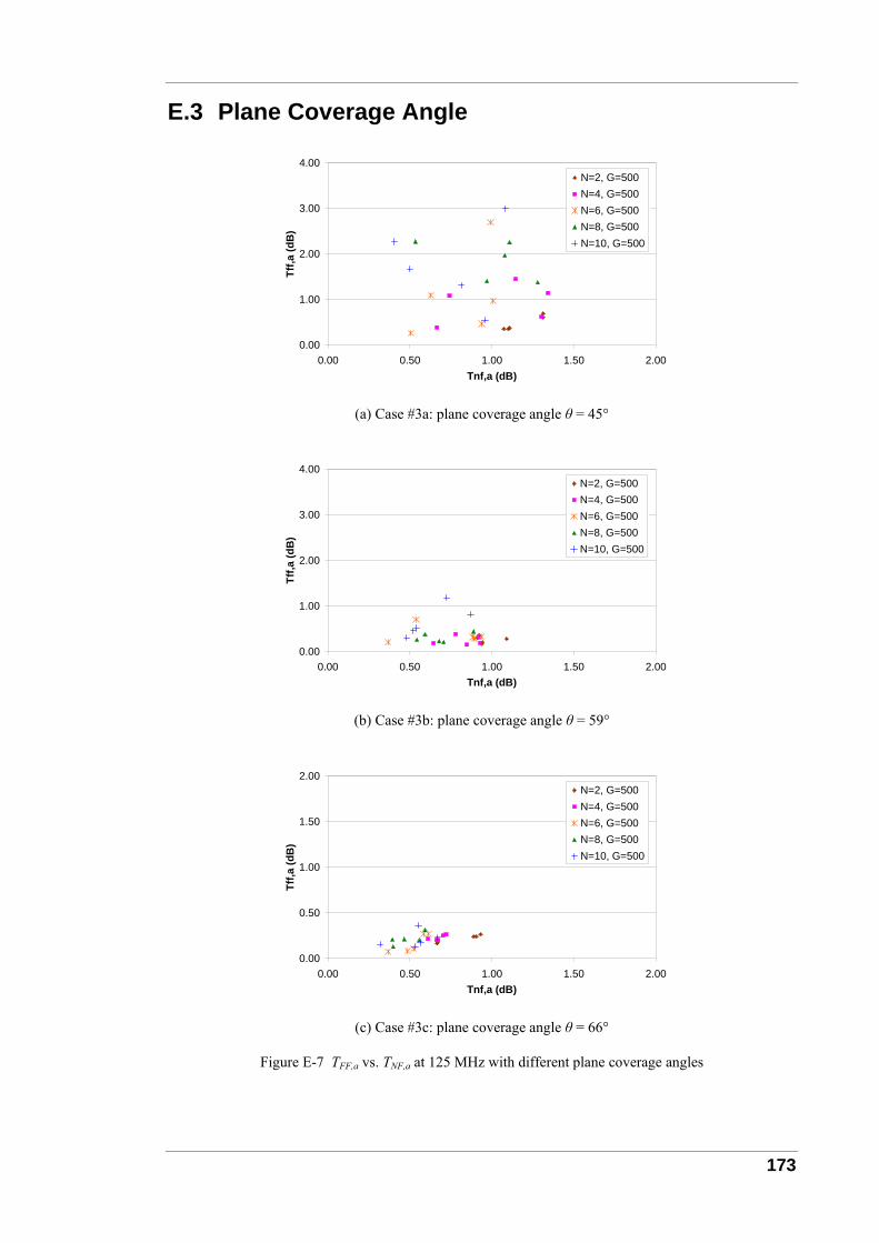
173

E.3 Plane Coverage Angle

0.00

1.00

2.00

3.00

4.00

0.00 0.50 1.00 1.50 2.00Tnf,a (dB)

Tff,a

(dB

)

N=2, G=500N=4, G=500N=6, G=500N=8, G=500N=10, G=500

(a) Case #3a: plane coverage angle θ = 45°

0.00

1.00

2.00

3.00

4.00

0.00 0.50 1.00 1.50 2.00Tnf,a (dB)

Tff,a

(dB

)

N=2, G=500N=4, G=500N=6, G=500N=8, G=500N=10, G=500

(b) Case #3b: plane coverage angle θ = 59°

0.00

0.50

1.00

1.50

2.00

0.00 0.50 1.00 1.50 2.00Tnf,a (dB)

Tff,a

(dB

)

N=2, G=500N=4, G=500N=6, G=500N=8, G=500N=10, G=500

(c) Case #3c: plane coverage angle θ = 66°

Figure E-7 TFF,a vs. TNF,a at 125 MHz with different plane coverage angles

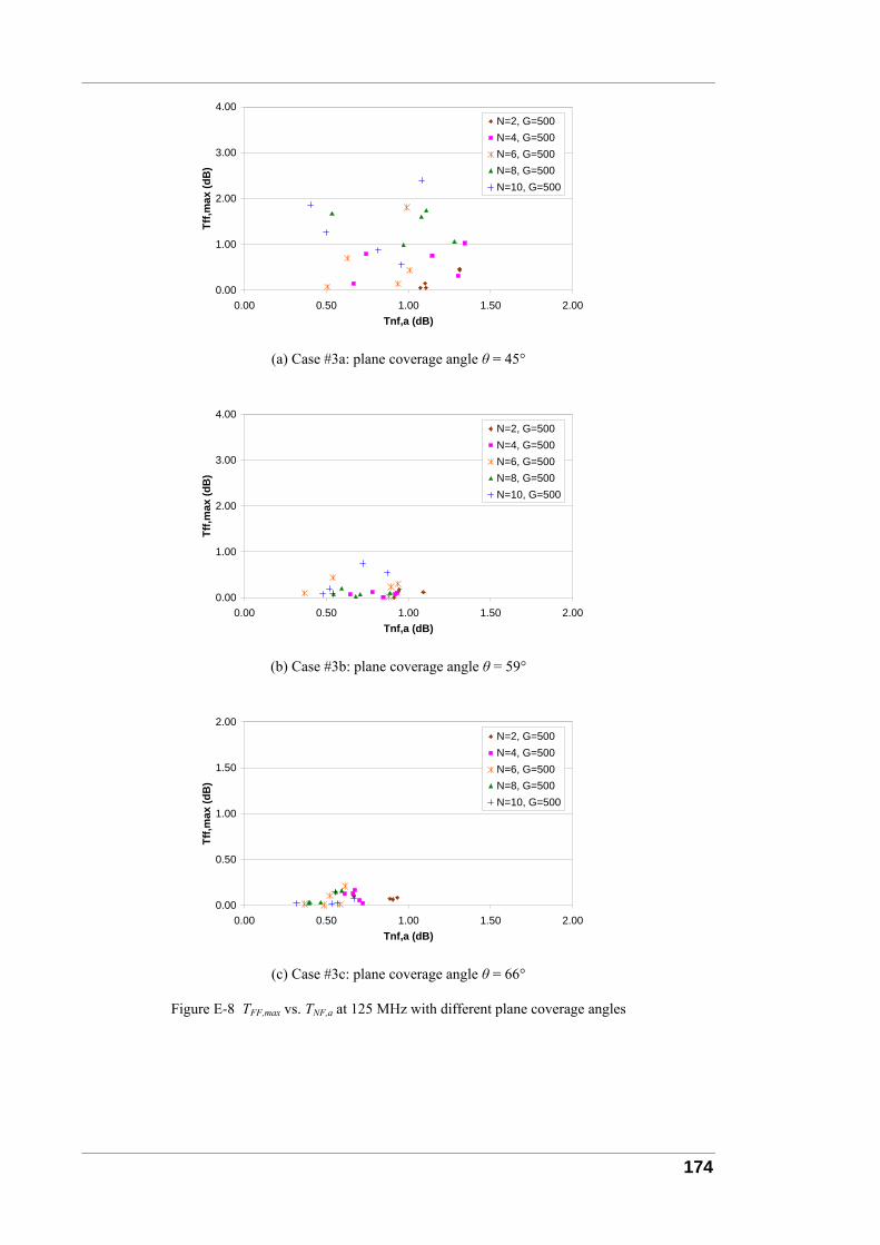
174

0.00

1.00

2.00

3.00

4.00

0.00 0.50 1.00 1.50 2.00Tnf,a (dB)

Tff,m

ax (d

B)

N=2, G=500N=4, G=500N=6, G=500N=8, G=500N=10, G=500

(a) Case #3a: plane coverage angle θ = 45°

0.00

1.00

2.00

3.00

4.00

0.00 0.50 1.00 1.50 2.00Tnf,a (dB)

Tff,m

ax (d

B)

N=2, G=500N=4, G=500N=6, G=500N=8, G=500N=10, G=500

(b) Case #3b: plane coverage angle θ = 59°

0.00

0.50

1.00

1.50

2.00

0.00 0.50 1.00 1.50 2.00Tnf,a (dB)

Tff,m

ax (d

B)

N=2, G=500N=4, G=500N=6, G=500N=8, G=500N=10, G=500

(c) Case #3c: plane coverage angle θ = 66°

Figure E-8 TFF,max vs. TNF,a at 125 MHz with different plane coverage angles

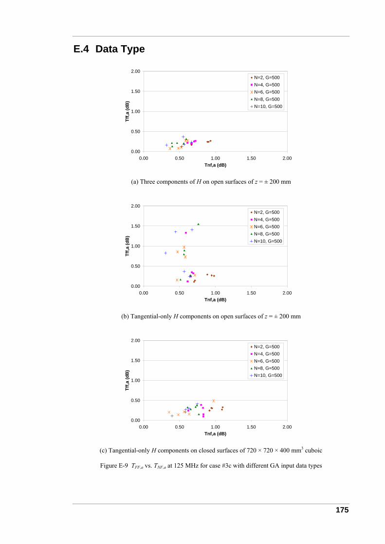
175

E.4 Data Type

0.00

0.50

1.00

1.50

2.00

0.00 0.50 1.00 1.50 2.00Tnf,a (dB)

Tff,a

(dB

)

N=2, G=500N=4, G=500N=6, G=500N=8, G=500N=10, G=500

(a) Three components of H on open surfaces of z = ± 200 mm

0.00

0.50

1.00

1.50

2.00

0.00 0.50 1.00 1.50 2.00Tnf,a (dB)

Tff,a

(dB

)

N=2, G=500N=4, G=500N=6, G=500N=8, G=500N=10, G=500

(b) Tangential-only H components on open surfaces of z = ± 200 mm

0.00

0.50

1.00

1.50

2.00

0.00 0.50 1.00 1.50 2.00Tnf,a (dB)

Tff,a

(dB

)

N=2, G=500N=4, G=500N=6, G=500N=8, G=500N=10, G=500

(c) Tangential-only H components on closed surfaces of 720 × 720 × 400 mm3 cuboic

Figure E-9 TFF,a vs. TNF,a at 125 MHz for case #3c with different GA input data types

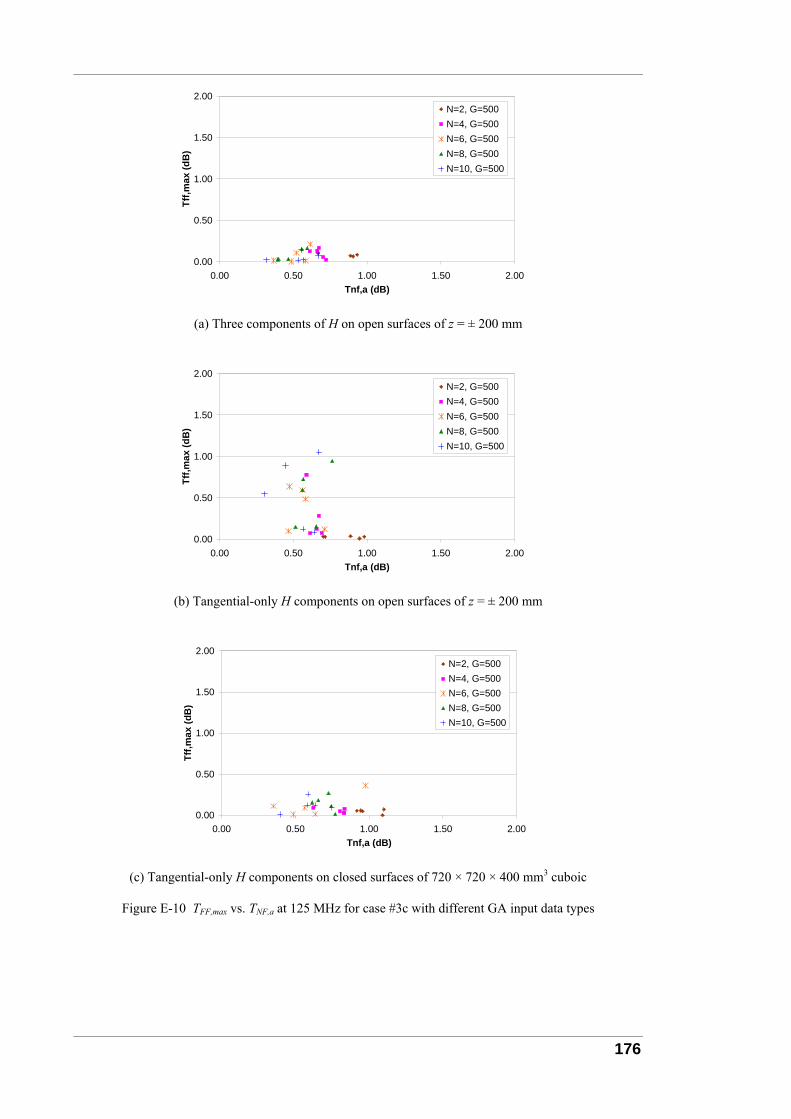
176

0.00

0.50

1.00

1.50

2.00

0.00 0.50 1.00 1.50 2.00Tnf,a (dB)

Tff,m

ax (d

B)

N=2, G=500N=4, G=500N=6, G=500N=8, G=500N=10, G=500

(a) Three components of H on open surfaces of z = ± 200 mm

0.00

0.50

1.00

1.50

2.00

0.00 0.50 1.00 1.50 2.00Tnf,a (dB)

Tff,m

ax (d

B)

N=2, G=500N=4, G=500N=6, G=500N=8, G=500N=10, G=500

(b) Tangential-only H components on open surfaces of z = ± 200 mm

0.00

0.50

1.00

1.50

2.00

0.00 0.50 1.00 1.50 2.00Tnf,a (dB)

Tff,m

ax (d

B)

N=2, G=500N=4, G=500N=6, G=500N=8, G=500N=10, G=500

(c) Tangential-only H components on closed surfaces of 720 × 720 × 400 mm3 cuboic

Figure E-10 TFF,max vs. TNF,a at 125 MHz for case #3c with different GA input data types

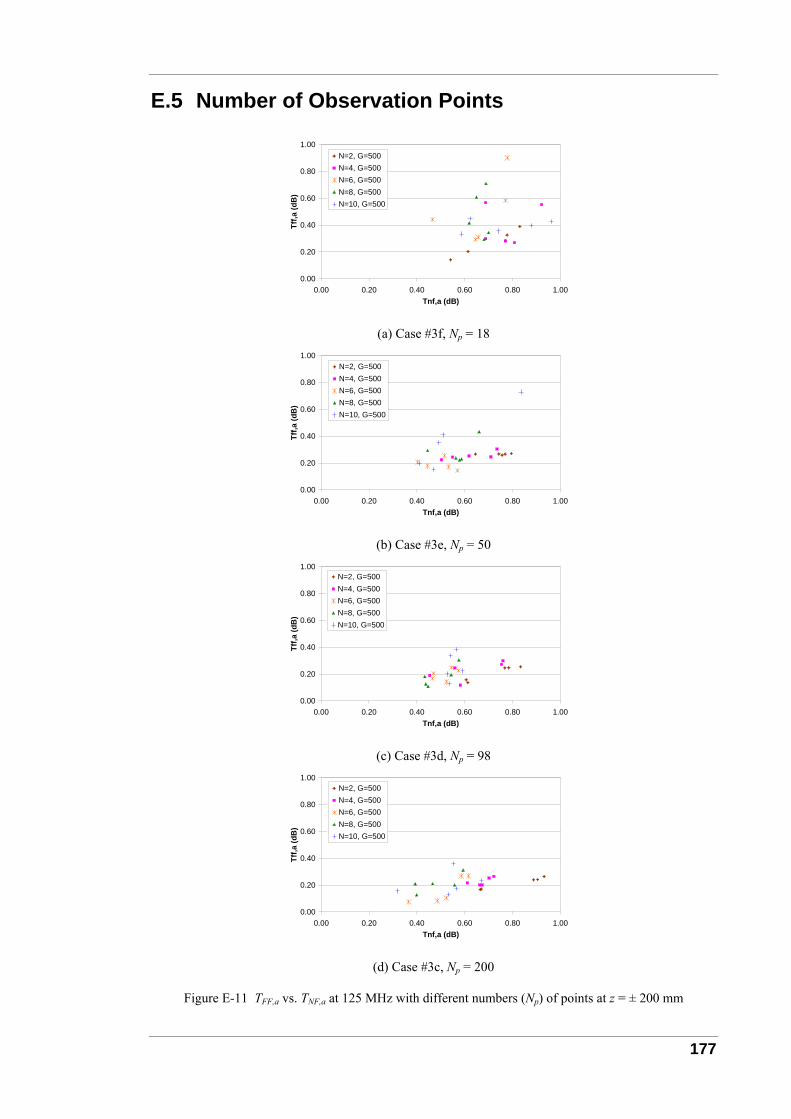
177

E.5 Number of Observation Points

0.00

0.20

0.40

0.60

0.80

1.00

0.00 0.20 0.40 0.60 0.80 1.00Tnf,a (dB)

Tff,a

(dB

)

N=2, G=500N=4, G=500N=6, G=500N=8, G=500N=10, G=500

(a) Case #3f, Np = 18

0.00

0.20

0.40

0.60

0.80

1.00

0.00 0.20 0.40 0.60 0.80 1.00Tnf,a (dB)

Tff,a

(dB

)

N=2, G=500N=4, G=500N=6, G=500N=8, G=500N=10, G=500

(b) Case #3e, Np = 50

0.00

0.20

0.40

0.60

0.80

1.00

0.00 0.20 0.40 0.60 0.80 1.00Tnf,a (dB)

Tff,a

(dB

)

N=2, G=500N=4, G=500N=6, G=500N=8, G=500N=10, G=500

(c) Case #3d, Np = 98

0.00

0.20

0.40

0.60

0.80

1.00

0.00 0.20 0.40 0.60 0.80 1.00Tnf,a (dB)

Tff,a

(dB

)

N=2, G=500N=4, G=500N=6, G=500N=8, G=500N=10, G=500

(d) Case #3c, Np = 200

Figure E-11 TFF,a vs. TNF,a at 125 MHz with different numbers (Np) of points at z = ± 200 mm

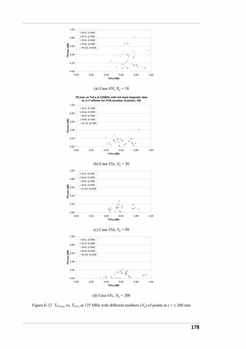
178

0.00

0.20

0.40

0.60

0.80

1.00

0.00 0.20 0.40 0.60 0.80 1.00Tnf,a (dB)

Tff,m

ax (d

B)

N=2, G=500N=4, G=500N=6, G=500N=8, G=500N=10, G=500

(a) Case #3f, Np = 18

Tff,max vs Tnf,a at 125MHz with GA input magnetic dataat z=+/-200mm for PCB (number of points: 50)

0.00

0.20

0.40

0.60

0.80

1.00

0.00 0.20 0.40 0.60 0.80 1.00Tnf,a (dB)

Tff,m

ax (d

B)

N=2, G=500N=4, G=500N=6, G=500N=8, G=500N=10, G=500

(b) Case #3e, Np = 50

0.00

0.20

0.40

0.60

0.80

1.00

0.00 0.20 0.40 0.60 0.80 1.00Tnf,a (dB)

Tff,m

ax (d

B)

N=2, G=500N=4, G=500N=6, G=500N=8, G=500N=10, G=500

(c) Case #3d, Np = 98

0.00

0.20

0.40

0.60

0.80

1.00

0.00 0.20 0.40 0.60 0.80 1.00Tnf,a (dB)

Tff,m

ax (d

B)

N=2, G=500N=4, G=500N=6, G=500N=8, G=500N=10, G=500

(d) Case #3c, Np = 200

Figure E-12 TFF,max vs. TNF,a at 125 MHz with different numbers (Np) of points at z = ± 200 mm

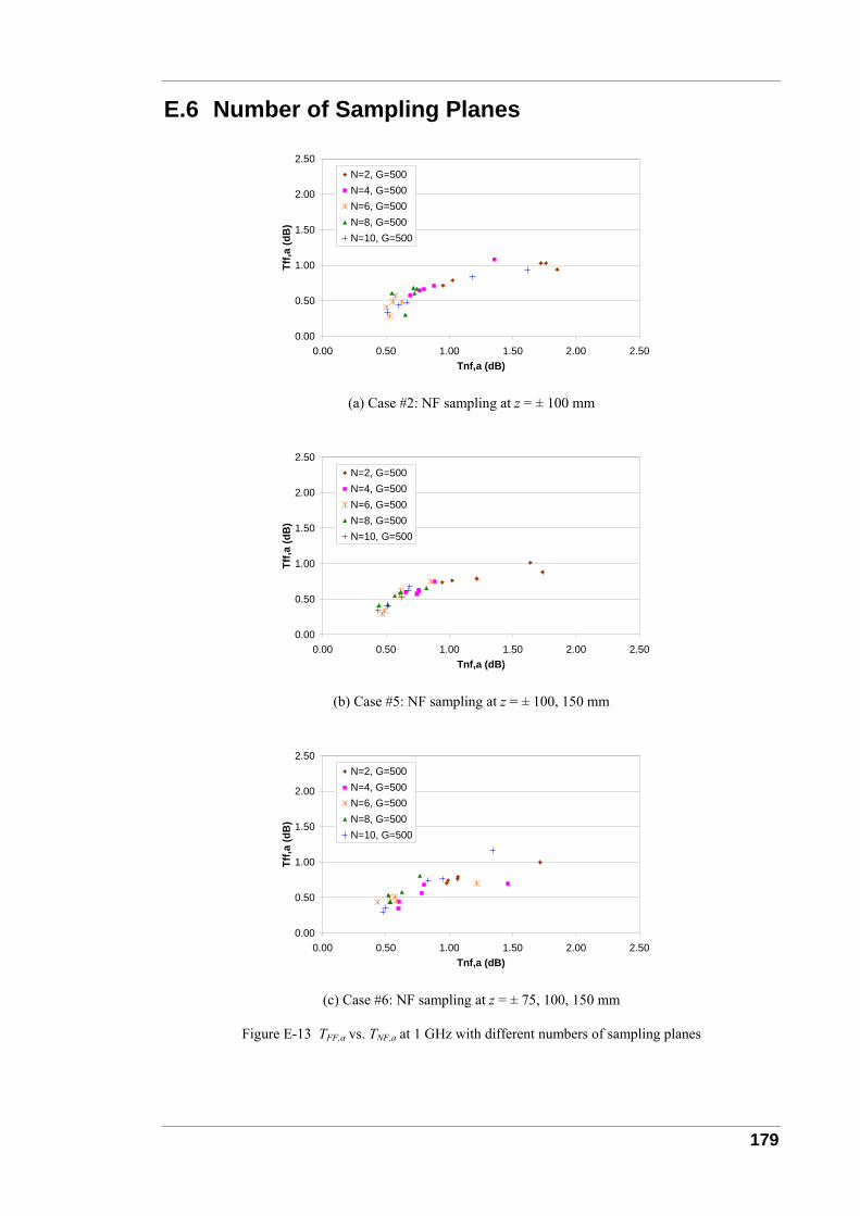
179

E.6 Number of Sampling Planes

0.00

0.50

1.00

1.50

2.00

2.50

0.00 0.50 1.00 1.50 2.00 2.50Tnf,a (dB)

Tff,a

(dB

)

N=2, G=500N=4, G=500N=6, G=500N=8, G=500N=10, G=500

(a) Case #2: NF sampling at z = ± 100 mm

0.00

0.50

1.00

1.50

2.00

2.50

0.00 0.50 1.00 1.50 2.00 2.50Tnf,a (dB)

Tff,a

(dB

)

N=2, G=500N=4, G=500N=6, G=500N=8, G=500N=10, G=500

(b) Case #5: NF sampling at z = ± 100, 150 mm

0.00

0.50

1.00

1.50

2.00

2.50

0.00 0.50 1.00 1.50 2.00 2.50Tnf,a (dB)

Tff,a

(dB

)

N=2, G=500N=4, G=500N=6, G=500N=8, G=500N=10, G=500

(c) Case #6: NF sampling at z = ± 75, 100, 150 mm

Figure E-13 TFF,a vs. TNF,a at 1 GHz with different numbers of sampling planes

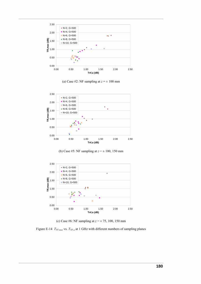
180

0.00

0.50

1.00

1.50

2.00

2.50

0.00 0.50 1.00 1.50 2.00 2.50Tnf,a (dB)

Tff,m

ax (d

B)

N=2, G=500N=4, G=500N=6, G=500N=8, G=500N=10, G=500

(a) Case #2: NF sampling at z = ± 100 mm

0.00

0.50

1.00

1.50

2.00

2.50

0.00 0.50 1.00 1.50 2.00 2.50Tnf,a (dB)

Tff,m

ax (d

B)

N=2, G=500N=4, G=500N=6, G=500N=8, G=500N=10, G=500

(b) Case #5: NF sampling at z = ± 100, 150 mm

0.00

0.50

1.00

1.50

2.00

2.50

0.00 0.50 1.00 1.50 2.00 2.50Tnf,a (dB)

Tff,m

ax (d

B)

N=2, G=500N=4, G=500N=6, G=500N=8, G=500N=10, G=500

(c) Case #6: NF sampling at z = ± 75, 100, 150 mm

Figure E-14 TFF,max vs. TNF,a at 1 GHz with different numbers of sampling planes

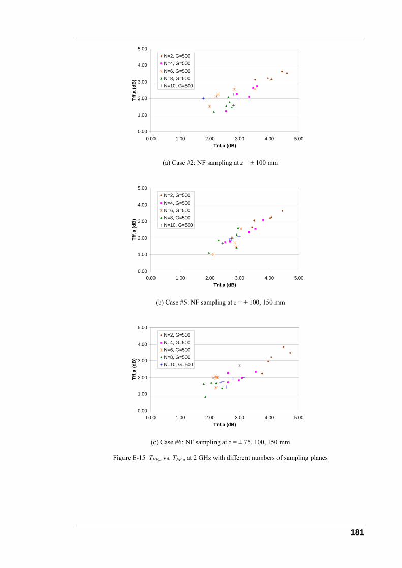
181

0.00

1.00

2.00

3.00

4.00

5.00

0.00 1.00 2.00 3.00 4.00 5.00Tnf,a (dB)

Tff,a

(dB

)

N=2, G=500N=4, G=500N=6, G=500N=8, G=500N=10, G=500

(a) Case #2: NF sampling at z = ± 100 mm

0.00

1.00

2.00

3.00

4.00

5.00

0.00 1.00 2.00 3.00 4.00 5.00Tnf,a (dB)

Tff,a

(dB

)

N=2, G=500N=4, G=500N=6, G=500N=8, G=500N=10, G=500

(b) Case #5: NF sampling at z = ± 100, 150 mm

0.00

1.00

2.00

3.00

4.00

5.00

0.00 1.00 2.00 3.00 4.00 5.00Tnf,a (dB)

Tff,a

(dB

)

N=2, G=500N=4, G=500N=6, G=500N=8, G=500N=10, G=500

(c) Case #6: NF sampling at z = ± 75, 100, 150 mm

Figure E-15 TFF,a vs. TNF,a at 2 GHz with different numbers of sampling planes

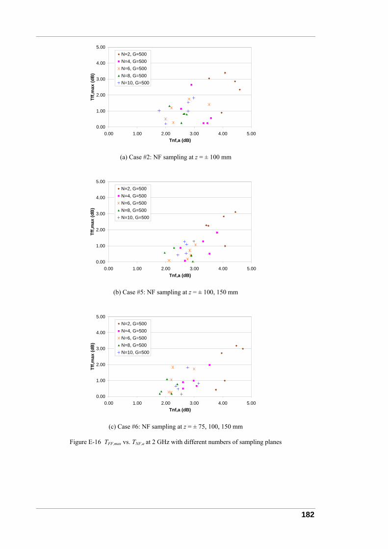
182

0.00

1.00

2.00

3.00

4.00

5.00

0.00 1.00 2.00 3.00 4.00 5.00Tnf,a (dB)

Tff,m

ax (d

B)

N=2, G=500N=4, G=500N=6, G=500N=8, G=500N=10, G=500

(a) Case #2: NF sampling at z = ± 100 mm

0.00

1.00

2.00

3.00

4.00

5.00

0.00 1.00 2.00 3.00 4.00 5.00Tnf,a (dB)

Tff,m

ax (d

B)

N=2, G=500N=4, G=500N=6, G=500N=8, G=500N=10, G=500

(b) Case #5: NF sampling at z = ± 100, 150 mm

0.00

1.00

2.00

3.00

4.00

5.00

0.00 1.00 2.00 3.00 4.00 5.00Tnf,a (dB)

Tff,m

ax (d

B)

N=2, G=500N=4, G=500N=6, G=500N=8, G=500N=10, G=500

(c) Case #6: NF sampling at z = ± 75, 100, 150 mm

Figure E-16 TFF,max vs. TNF,a at 2 GHz with different numbers of sampling planes

183

0.00

1.00

2.00

3.00

4.00

5.00

0.00 1.00 2.00 3.00 4.00 5.00Tnf,a (dB)

Tff,a

(dB

)

N=2, G=500N=4, G=500N=6, G=500N=8, G=500N=10, G=500

(a) Case #2: NF sampling at z = ± 100 mm

0.00

1.00

2.00

3.00

4.00

5.00

0.00 1.00 2.00 3.00 4.00 5.00Tnf,a (dB)

Tff,a

(dB

)

N=2, G=500N=4, G=500N=6, G=500N=8, G=500N=10, G=500

(b) Case #5: NF sampling at z = ± 100, 150 mm

0.00

1.00

2.00

3.00

4.00

5.00

0.00 1.00 2.00 3.00 4.00 5.00Tnf,a (dB)

Tff,a

(dB

)

N=2, G=500N=4, G=500N=6, G=500N=8, G=500N=10, G=500

(c) Case #6: NF sampling at z = ± 75, 100, 150 mm

Figure E-17 TFF,a vs. TNF,a at 3 GHz with different numbers of sampling planes

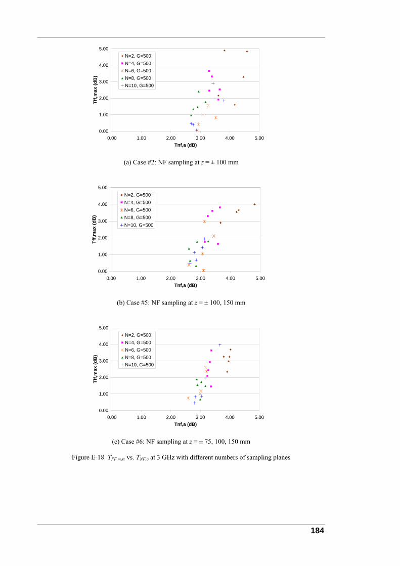
184

0.00

1.00

2.00

3.00

4.00

5.00

0.00 1.00 2.00 3.00 4.00 5.00Tnf,a (dB)

Tff,m

ax (d

B)

N=2, G=500N=4, G=500N=6, G=500N=8, G=500N=10, G=500

(a) Case #2: NF sampling at z = ± 100 mm

0.00

1.00

2.00

3.00

4.00

5.00

0.00 1.00 2.00 3.00 4.00 5.00Tnf,a (dB)

Tff,m

ax (d

B)

N=2, G=500N=4, G=500N=6, G=500N=8, G=500N=10, G=500

(b) Case #5: NF sampling at z = ± 100, 150 mm

0.00

1.00

2.00

3.00

4.00

5.00

0.00 1.00 2.00 3.00 4.00 5.00Tnf,a (dB)

Tff,m

ax (d

B)

N=2, G=500N=4, G=500N=6, G=500N=8, G=500N=10, G=500

(c) Case #6: NF sampling at z = ± 75, 100, 150 mm

Figure E-18 TFF,max vs. TNF,a at 3 GHz with different numbers of sampling planes

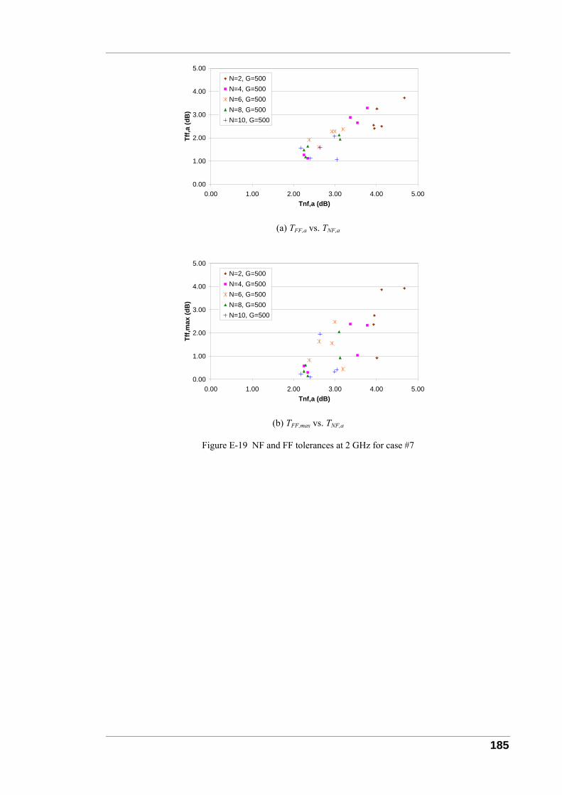
185

0.00

1.00

2.00

3.00

4.00

5.00

0.00 1.00 2.00 3.00 4.00 5.00Tnf,a (dB)

Tff,a

(dB

)

N=2, G=500N=4, G=500N=6, G=500N=8, G=500N=10, G=500

(a) TFF,a vs. TNF,a

0.00

1.00

2.00

3.00

4.00

5.00

0.00 1.00 2.00 3.00 4.00 5.00Tnf,a (dB)

Tff,m

ax (d

B)

N=2, G=500N=4, G=500N=6, G=500N=8, G=500N=10, G=500

(b) TFF,max vs. TNF,a

Figure E-19 NF and FF tolerances at 2 GHz for case #7

186

Appendix F Author Biography

F.1 Author Publications

1) H. Fan: Using Radiating Near Field Region to Sample Radiation of Microstrip

Traces for Far Field Prediction by Genetic Algorithms, IEEE Microwave and

Wireless Components Letters, vol. 19, no. 5, 2009, pp. 272-274 [50].

2) H. Fan, F. Schlagenhaufer: Source Identification and Correlation between Near

Field-Far Field Tolerances when Applying a Genetic Algorithm, EMC Europe

Int. Symp. EMC, Hamburg, Sept. 2008, pp. 587-592 [49].

3) H. Fan, F. Schlagenhaufer: Number of Infinitesimal Dipoles in Genetic

Algorithms for Near Field-Far Field Conversion, 1st Asia-Pacific Symp. EMC,

Singapore, May 2008, pp. 690-693 [48].

4) H. Fan, F. Schlagenhaufer: Investigation of Near Field Data Sampling

Approaches for Far Field Radiation Prediction of PCBs by Genetic Algorithm,

18th Int. Zurich Symp. EMC, Munich, Sept. 2007, pp. 21-24 [47].

5) H. Fan, F. Schlagenhaufer: Modelling of Fitness Definition of Near Field

Matching & Far Field Prediction Based on Genetic Algorithm, 6th Australian

Symp. EMC, Melbourne, Sept. 2007, pp. 35-41 [46].

6) H. Fan, F. Schlagenhaufer: Improvements of Robustness of Genetic Algorithm

for Near Field-Far Field Radiation Conversion, IEEE 2007 Int. Symp.

Microwave, Antenna, Propagation and EMC Technologies for Wireless

Communications, Hangzhou, Aug. 2007, pp. 950-953 [45].

7) H. Fan, F. Schlagenhaufer: Near Field-Far Field Conversion Based on Genetic

Algorithm for Predicting Radiation from PCBs, 2007 IEEE Int. Symp. EMC,

Honolulu, Jul. 2007 [44].

8) H. Fan, F. Schlagenhaufer: Source Identification from Near Field Measurements

of Loops Using Genetic Algorithm, 5th Australian Symp. EMC, Melbourne, Sept.

2006, pp. 35-42 [43].

187

9) H. Fan, F. Schlagenhaufer: Near Field-Far Field Transformation for Loops

Based on Genetic Algorithm, 4th Asia-Pacific Conf. Environmental

Electromagnetics, Dalian, Aug. 2006, pp. 476-481 [42].

F.2 Awards Received

Duration Award Organisation Name

Mar 2009 EMCSA Student Paper Prize The EMC Society of Australia

Mar 2006 –

Aug 2008

Samaha Research Scholarship Faculty of Engineering, Computing and

Mathematics, The University of Western

Australia (UWA)

May 2008 UWA Grants for Research

Student Training

Graduate Research School, UWA

Jul 2007 Graduate Research Student

Travel Award

Graduate Research School, UWA

Jul 2007 Postgraduate Travel Award School of Electrical, Electronics and

Computer Engineering, UWA

Jun 2007 PSA Conference Travel Award The Postgraduate Students’ Association,

UWA

Sept 2006 EMCSA Student Project Grant The EMC Society of Australia

188

References

[1] CONCEPT: www.tet.tu-harburg.de/en_EN

[2] C. A. Balanis: Antenna Theory: Analysis and Design, John Wiley & Sons, Inc.,

Hoboken, 2005 (www.wiley.com/engineering).

[3] R. F. Harrington: Time-Harmonic Electromagnetic Fields, McGraw-Hill Book

Company, Inc., New York, 1961.

[4] C. A. Balanis: Advanced Engineering Electromagnetics, John Wiley & Sons, Inc.,

New York, 1989.

[5] M. Sadiku: Elements of Electromagnetics, Oxford University Press, New York,

Oxford, 2001 (www.oup.com).

[6] R. F. Harrington: Field Computation by Moment Methods, IEEE Press,

Piscataway, 1993.

[7] L. S. Taylor: The Phase Retrieval Problem, IEEE Trans. Antennas Propag., vol.

AP-29, no. 2, 1981, pp. 386-391.

[8] J. R. Fienup: Phase Retrieval Algorithms: A Comparison, Appl. Opt., vol. 21, no.

15, 1982, pp. 2758-2769.

[9] M. Wehr, G. Mönich: Detection of Radiation Leaks by Spherically Scanned Field

Data, 10th Int. Zurich Symp. EMC, 1993, pp. 337-342.

[10] M. Wehr, A. Podubrin, G. Mönich: Automatized Search for Models by Evolution

Strategy to Characterize Radiators, 11th Int. Zurich Symp. EMC, 1995, pp. 27-34.

[11] J. Regue, M. Ribo, J. Garrell, S. Sorroche, J. Ayuso: A Genetic Algorithm Based

Method for Predicting Far-Field Radiated Emissions from Near-Field

Measurements, 2000 IEEE Int. Symp. EMC, Washington DC, Aug. 2000, pp. 147-

151.

[12] J. Regue, M. Ribo, J. Garrell, A. Martin: A Genetic Algorithm Based Method for

Source Identification and Far-Field Radiated Emissions Prediction from Near-

Field Measurements for PCB Characterization, IEEE Trans. EMC, vol. 43, no. 4,

2001, pp. 520-530.

189

[13] J. Regue, M. Ribo, J. Gomila, A. Perez, A. Martin: Modeling of Radiating

Equipment by Distributed Dipoles Using Metaheuristic Methods, IEEE Int. Symp.

EMC, Chicago, Aug. 2005, pp. 596-601.

[14] R. Laroussi, G. I. Costache: Novel Technique for Radiated Far-Field Predictions

from Near-Field Measurements, IEEE 1992 Asia-Pacific Microwave Conf.,

Adelaide, 1992, pp. 791-794.

[15] R. Laroussi, G. I. Costache: Far-Field Predictions from Near-Field Measurements

Using an Exact Integral Equation Solution, IEEE Trans. EMC, vol. 36, no. 3,

1994, pp. 189-195.

[16] P. Petre, T. K. Sarkar: Planar Near-Field to Far-Field Transformation Using an

Equivalent Magnetic Current Approach, IEEE Trans. Antennas Propag., vol. 40,

no. 10, 1992, pp. 1348-1356.

[17] P. Petre, T. K. Sarkar: Planar Near-Field to Far-Field Transformation Using an

Array of Dipole Probes, IEEE Trans. Antennas Propag., vol. 42, no. 4, 1994, pp.

534-537.

[18] A. Taaghol, T. K. Sarkar: Near-Field to Near/Far-Field Transformation for

Arbitrary Near-Field Geometry, Utilizing an Equivalent Magnetic Current, IEEE

Trans. EMC, vol. 38, no. 3, 1996, pp. 536-542.

[19] T. K. Sarkar, F. Las-Heras: An Interactive Spherical Near-Field to Far-Field

Emissions and Source Reconstruction Using the Equivalent Current Approach,

2001 IEEE Int. Symp. EMC, Montreal, Aug. 2001, pp. 395-398.

[20] T. K. Sarkar, A. Taaghol: Near-Field to Near/Far-Field Transformation for

Arbitrary Near-Field Geometry Utilizing an Equivalent Electric Current and

MoM, IEEE Trans. Antennas Propag., vol. 47, no. 3, 1999, pp. 566-573.

[21] J. J. Laurin, J. Zurcher, F. E. Gardiol: Near-Field Diagnostics of Small Printed

Antennas Using the Equivalent Magnetic Current Approach, IEEE Trans.

Antennas Propag., vol. 49, no. 5, 2001, pp. 814-828.

[22] O. M. Bucci, G. D’Elia, G. Leone, R. Pierri: Far-Field Pattern Determination

from the Near-Field Magnitude on Two Surfaces, IEEE Trans. Antennas Propag.,

vol. 38, no. 11, 1990, pp. 1772-1779.

190

[23] O. M. Bucci, G. D’Elia, G. Leone, R. Pierri: Far-field Computation from

Magnitude Near-Field Data on Two Surfaces: Cylindrical Case, IEE Proc. Part H:

Microwaves, Antennas and Propagation, vol. 139, no. 2, 1992, pp. 143-148.

[24] T. Isernia, G. Leone, R. Pierri: Radiation Pattern Evaluation from Near-Field

Intensities on Planes, IEEE Trans. Antennas Propag., vol. 44, no. 5, 1996, pp.

701-710.

[25] R. G. Yaccarino, Y. Rahmat-Samii : Phaseless Bi-Polar Planar Near-Field

Measurements and Diagnostics of Array Antennas, IEEE Trans. Antennas

Propag., vol. 47, no. 3, 1999, pp. 574-583.

[26] M. D. Migliore, F. Soldovieri, R. Pierri: Far-Field Antenna Pattern Estimation

from Near-Field Data Using a Low-Cost Magnitude-Only Measurement Setup,

IEEE Trans. Instrum. Meas., vol. 49, no. 1, 2000, pp. 71-76.

[27] R. Pierri, G. D’Elia, F. Soldovieri : A Two Probes Scanning Phaseless Near-Field

Far-Field Transformation Technique, IEEE Trans. Antennas Propag., vol. 47, no.

5, 1999, pp. 792-802.

[28] O. M. Bucci, G. D’Elia, M. D. Migliore: An Effective Near-Field Far-Field

Transformation Technique from Truncated and Inaccurate Magnitude-Only Data,

IEEE Trans. on Antennas Propag., vol. 47. no. 9, 1999, pp. 1377-1385.

[29] F. Las-Heras, T. K. Sarkar: A Direct Optimization Approach for Source

Reconstruction and NF-FF Transformation Using Magnitude-Only Data, IEEE

Trans. on Antennas Propag., vol. 50, no. 4, 2002, pp. 500-510.

[30] A. Hoorfar: Evolutionary Programming in Electromagnetic Optimization: A

Review, IEEE Trans. on Antennas Propag., vol. 55. no. 3, 2007, pp. 523-537.

[31] D. E. Goldberg: Genetic Algorithms in Search, Optimization & Machine Learning,

Addison-Wesley Publishing Company, Inc., Reading, 1989.

[32] Z. Michalewicz: Genetic Algorithms + Data Structures = Evolution Programs,

Springer-Verlag, Berlin, 1992.

[33] J. R. Perez, J. Basterechea: Prediction of DUT radiation from Near-Field

measurements in a screened room using GAs, 2001 IEEE Int. Symp. EMC,

Montreal, Aug. 2001, pp. 383-388.

191

[34] M. B. Margari, M. Baroni, F. Marliani, F. Canavero: Modeling of Electromagnetic

Sources by Means of a Genetic Algorithm, 16th Int. Zurich Workshops & Tutorials

on EMC, Zurich, Feb. 2005, pp. 86-98.

[35] T. S. Sijher, A. A. Kishk: Antenna Modeling by Infinitesimal Dipoles Using

Genetic Algorithms, Progress in Electromagnetics Research, PIER 52, 2005, pp.

225-254.

[36] J. H. Holland: Adaptation in Natural and Artificial Systems, University of

Michigan Press, Ann Arbor, 1975.

[37] N. Chaiyaratana, A. M. S. Zalzala: Recent Developments in Evolutionary and

Genetic Algorithms: Theory and Applications, IEE 2nd Int. Conf. Genetic

Algorithms in Engineering Systems: Innovations and Applications, Glasgow, Sept.

1997, pp. 270-277.

[38] J. M. Johnson, Y. Rahmat-Samii: Genetic Algorithms in Engineering

Electromagnetics, IEEE Trans. Antennas Propag., vol. 39, no. 4, 1997, pp. 7-21.

[39] D. S. Weile, E. Michielssen: Genetic Algorithm Optimization Applied to

Electromagnetics: A Review, IEEE Trans. Antennas Propag., vol. 45, no. 3, 1997,

pp. 343-353.

[40] Y. Rahmat-Samii, E. Michielssen: Electromagnetic Optimization by Genetic

Algorithms, John Wiley & Sons, Inc., New York, 1999.

[41] D. Plettmeier, S. Balling, D. Landmann, K. -H. Gonschorek, Consert-Team: Use

of Genetic Algorithms to Solve Inverse Scattering Problems, 2007 IEEE Int.

Symp. EMC, Honolulu, Jul. 2007.

[42] H. Fan, F. Schlagenhaufer: Near Field-Far Field Transformation for Loops Based

on Genetic Algorithm, 4th Asia-Pacific Conf. Environmental Electromagnetics,

Dalian, Aug. 2006, pp. 476-481.

[43] H. Fan, F. Schlagenhaufer: Source Identification from Near Field Measurements

of Loops Using Genetic Algorithm, 5th Australian Symp. EMC, Melbourne, Sept.

2006, pp. 35-42.

192

[44] H. Fan, F. Schlagenhaufer: Near Field-Far Field Conversion Based on Genetic

Algorithm for Predicting Radiation from PCBs, 2007 IEEE Int. Symp. EMC,

Honolulu, Jul. 2007.

[45] H. Fan, F. Schlagenhaufer: Improvements of Robustness of Genetic Algorithm for

Near Field-Far Field Radiation Conversion, 2007 IEEE Int. Symp. Microwave,

Antenna, Propagation and EMC Technologies for Wireless Communications,

Hangzhou, Aug. 2007, pp. 950-953.

[46] H. Fan, F. Schlagenhaufer: Modelling of Fitness Definition of Near Field

Matching & Far Field Prediction Based on Genetic Algorithm, 6th Australian

Symp. EMC, Melbourne, Sept. 2007, pp. 35-41.

[47] H. Fan, F. Schlagenhaufer: Investigation of Near Field Data Sampling

Approaches for Far Field Radiation Prediction of PCBs by Genetic Algorithm,

18th Int. Zurich Symp. EMC, Munich, Sept. 2007, pp. 21-24.

[48] H. Fan, F. Schlagenhaufer: Number of Infinitesimal Dipoles in Genetic Algorithms

for Near Field-Far Field Conversion, 1st Asia-Pacific Symp. EMC, Singapore,

May 2008, pp. 690-693.

[49] H. Fan, F. Schlagenhaufer: Source Identification and Correlation between Near

Field-Far Field Tolerances when Applying a Genetic Algorithm, EMC Europe Int.

Symp. EMC, Hamburg, Sept. 2008, pp. 587-592.

[50] H. Fan: Using Radiating Near Field Region to Sample Radiation of Microstrip

Traces for Far Field Prediction by Genetic Algorithms, IEEE Microwave and

Wireless Components Letters, vol. 19, no. 5, 2009, pp. 272-274.

[51] C. A. Coello Coello, D. A. Van Veldhuizen, G. B. Lamont: Evolutionary

Algorithms for solving Multi-Objective problems, Kluwer Academic / Plenum

Publishers, New York, 2002 (www.wkap.com).

[52] W. L. Stutzman, G. A. Thiele, Antenna Theory and Design, John Wiley & Sons,

Inc., New York, 1998 (www.wiley.com/college).

[53] J. D. Kraus, R. J. Marhefka: Antennas: for All Applications, McGraw-Hill Higher

Education, New York, 2002 (www.mhhe.com).

193

[54] A. D. Yaghjian: An Overview of Near-Field Antenna Measurements, IEEE Trans.

Antennas Propag., vol. 34, no. 1, 1986, pp. 30-45.

[55] G. -T. Lei, R. W. Techentin, B. K. Gilbert, High-Frequency Characterization of

Power/Ground-Plane Structures, IEEE Trans. Microw. Theory Tech., vol. 47, no.

5, 1999, pp. 562-569.

[56] T. Fischer, M. Leone, M. Albach: An Analytical Model for Studying the

Electromagnetic Radiation of Power-Bus Structures, 2003 IEEE Int. Symp. EMC,

Boston, Aug. 2003, pp. 225-230.

[57] M. Leone: The Radiation of a Rectangular Power-Bus Structure at Multiple

Cavity-Mode Resonances, IEEE Trans. EMC, vol. 45, no. 3, 2003, pp. 486-492.

[58] EMSCAN: www.EMSCAN.com

[59] Detectus AB: www.detectus.se

[60] K. L. Kaiser: Electromagnetic Compatibility Handbook, CRC Press, Boca Raton,

2005 (www.crcpress.com).