Correlation and Regression - Cornell University · Correlation, Regression, etc. 1 Topics...
175
Introduction to Correlation and Regression D G Rossiter February 17, 2016 Copyright 2007–2012, 2015-16 D G Rossiter All rights reserved. Reproduction and dissemination of the work as a whole (not parts) freely permitted if this original copyright notice is included. Sale or placement on a web site where payment must be made to access this document is strictly prohibited. To adapt or translate please contact the author ([email protected]).
Transcript of Correlation and Regression - Cornell University · Correlation, Regression, etc. 1 Topics...
Introduction to Correlation and Regression
D G Rossiter
February 17, 2016
Copyright © 2007–2012, 2015-16 D G RossiterAll rights reserved. Reproduction and dissemination of the work as a whole (not parts) freely permitted if this originalcopyright notice is included. Sale or placement on a web site where payment must be made to access this document is strictlyprohibited. To adapt or translate please contact the author ([email protected]).
Correlation, Regression, etc. 1
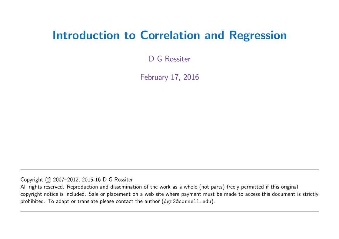
Topics
1. Correlation
2. Simple linear regression
3. Model validation
4. Structural analysis
5. Multiple linear regression
6. Regression trees and random forests
7. Factor analysis (Principal Components Analysis)
8. Robust methods
D G Rossiter

Correlation, Regression, etc. 2
Computing environment
Output produced by R; see http://www.r-project.org
D G Rossiter
Correlation, Regression, etc. 3
Topic: Relations between variables
Given a dataset which contains:
� sampling units (“records”, “individuals”)
� items measured on each sampling unit (“variables”)
What is the “relation” between the variables?
� Association: what?
� Explanation: why?
� Causation: how?
� Prediction: what if?
D G Rossiter
Correlation, Regression, etc. 4
Types of relations between variables
1. Variables are of equal status
(a) A bivariate correlation between two variables;(b) A multivariate correlation between several variables;(c) A structural relation between two variables;(d) A structural relation between several variables (e.g. principal components).
2. Variables have different status
(a) A simple regression of one dependent variable on one independent variable;(b) A multiple regression of one dependent variable on several independent
variable.(c) A hierachical model (tree) relating a dependent variable to several independent
variables.
D G Rossiter
Correlation, Regression, etc. 5
Regression
This is a general term for modelling one or more:
� response variables (predictands, mathematically dependent), from one or more
� predictor variables (mathematically independent)
Note: The “response” and “predictor” are mathematical terms, not necessarily “effect”and“cause”– that requires meta-statistical reasoning.
D G Rossiter
Correlation, Regression, etc. 6
Linear models
� All variables are related with linear equations.
� These are easy to work with and have good mathematical properties.
� Their interpretation is easy (proportional relations).
� The linear relation can be after transformation of one or more variables, to linearizethe relation.
� Relations that can not be linearized are intrinsically non-linear.
D G Rossiter
Correlation, Regression, etc. 7
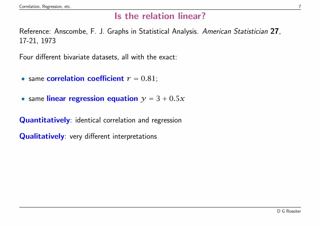
Is the relation linear?
Reference: Anscombe, F. J. Graphs in Statistical Analysis. American Statistician 27,17-21, 1973
Four different bivariate datasets, all with the exact:
� same correlation coefficient r = 0.81;
� same linear regression equation y = 3+ 0.5x
Quantitatively: identical correlation and regression
Qualitatively: very different interpretations
D G Rossiter
Correlation, Regression, etc. 8
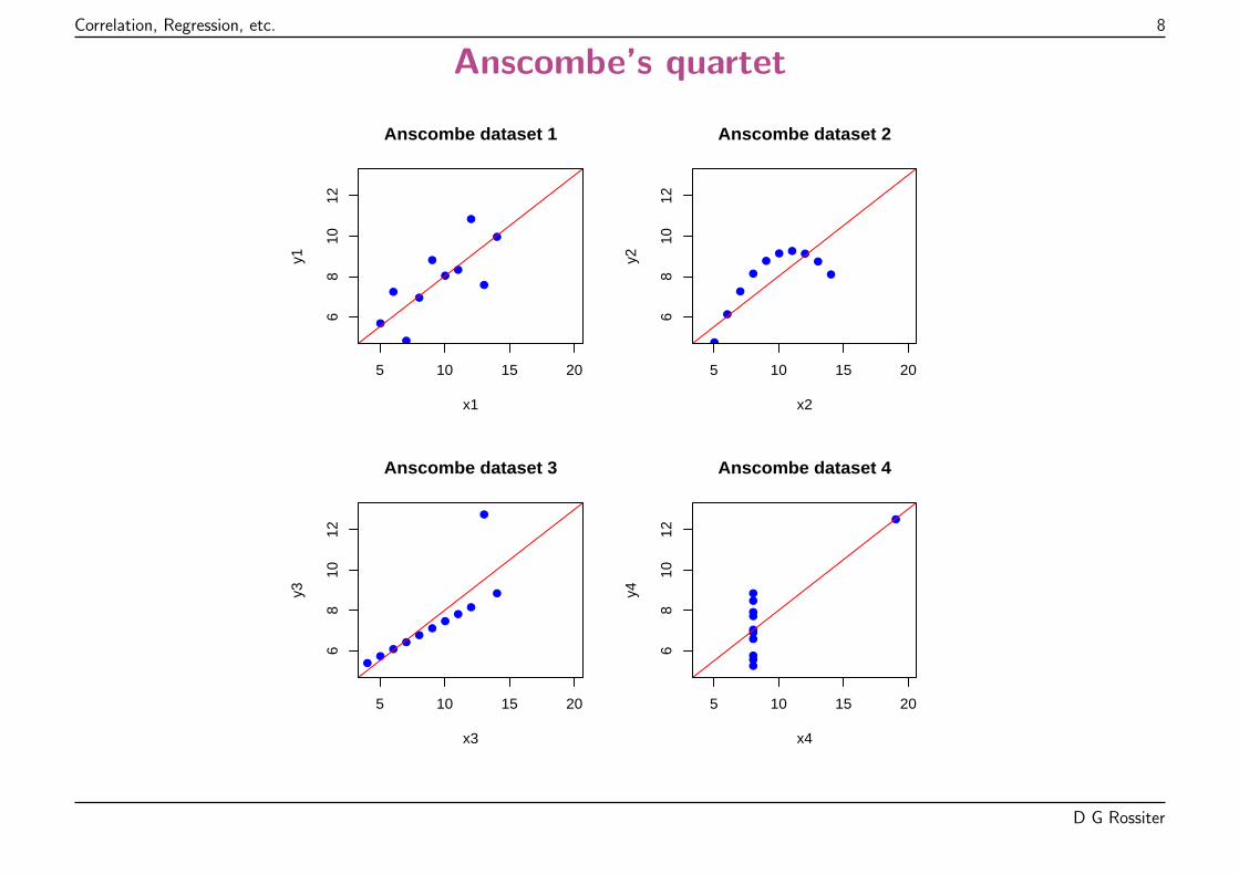
Anscombe’s quartet
●
●
●
●●
●
●
●
●
●
5 10 15 20
68
1012
x1
y1
Anscombe dataset 1
●
●
●●●
●
●
●
●
●
5 10 15 20
68
1012
x2
y2
Anscombe dataset 2
●
●
●
●
●
●
●
●
●
●
●
5 10 15 20
68
1012
x3
y3
Anscombe dataset 3
●
●
●
●●
●
●
●
●
●
●
5 10 15 20
68
1012
x4
y4
Anscombe dataset 4
D G Rossiter
Correlation, Regression, etc. 9
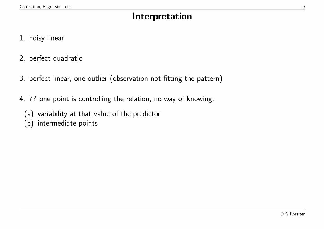
Interpretation
1. noisy linear
2. perfect quadratic
3. perfect linear, one outlier (observation not fitting the pattern)
4. ?? one point is controlling the relation, no way of knowing:
(a) variability at that value of the predictor(b) intermediate points
D G Rossiter
Correlation, Regression, etc. 10
Topic: Correlation
� Measures the strength of association between two variables measured on the sameobject:
* −1 (perfect negative correlation)* 0 (no correlation)* +1 (perfect positive correlation).
� The two variables have logically equal status
� No concept of causation
� No functional relation, no way to predict
D G Rossiter
Correlation, Regression, etc. 11
Example dataset
Source: W B Mercer and A D Hall. The experimental error of field trials. The Journal ofAgricultural Science (Cambridge), 4: 107–132, 1911.
� A uniformity trial: 500 supposedly identical plots within one field
� All planted to one variety of wheat and treated identically
� Measured variables: grain and straw yields, lbs per plot, precision of 0.01 lb(0.00454 kg)
D G Rossiter
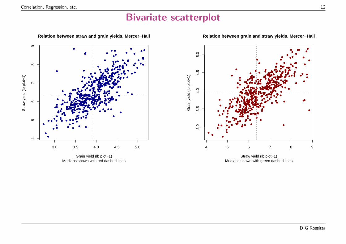
Correlation, Regression, etc. 12
Bivariate scatterplot
●
●
●
●
●
●
●
●
●
●●
● ●●
●
●
●
●
●
●
●
●
●
●
●
●
●
●
●
●●
●
●
●
●
●
●
●
●
●
●
●●
●
●
● ●●
●
●
●
●
●
●
●
●
●
●
●
●
●
●
●
●
●●
●
●
●●
●
●
●
●
●
●
●
●
●●
●
●
●
●
●
●
●
●
●
●
●
●
● ●
●
●
●
●
●
●
●
●
●
●
●
●● ●
● ●
●
●
●
●
●
●
●●
●
●
●
●
●
●
●
●
●
●
●
●
●
●
●
●
●
●
●●
●
●
●
●
●
●●
●
●
●
●
●
●●
●●
●
●
●
●
●
●
●●
●
●
●
●
●
●
●●
●
●●
●
●
●
●
●
●●
●
●
●
●
●
●
●●
●
●● ●●
●
●
●
●
●
●
●
●
●●
●
●
●
●●
●
●
●
●
●
●
●
●
●
●
●
●
●
●●
●
●
●
●
●
●
●
●
●
●
●
●
●
●
●
●
●
●
●
●
●●
●
●
●
●
●
●
●
●
●
●
●
●
●
●
●
●
●
●
●
●
●●
●
●
●●
●
● ●
●
●
●
●
●
●
●
●
●
●
●
●
●
●
●
●
●●
●
●
●
●
●
●
●
● ●
●
●
●
●
●
●
●
●
●
●
●
●
●
●
●
●
●
●●
●●
●
●
●
●
●
●
●
●
●
●
●
●
●
●
●
●
●
●
●
●
●
●
●
●
●
●
●●●
●
●●
●
●
●
●
●
●
●
●
●
●
●
●
●
●
●
●
●
●
●
●
●●
● ●
●
●
●
●
●
●
●
●
●
●
●●
●
●
●
●
● ●●
●
●
●
●
●
●●
● ●
●
●●
●
●
●
●
● ●
●
●●
●
●
●
●
●
●
●
●
●
●
●●
●●
●
●
●
●
●
● ●●
●
●
●
●
●
●
●
●
●●
●
●
●
●
●
●
●●
●
●
●
●
●
●
●●
●
●
●
●
●
●
●●●
●
●
●
●
●
●
●
●
● ●
●
●
●
●
●
●
●
●
●
●
●
●
●
●
●
3.0 3.5 4.0 4.5 5.0
45
67
89
Relation between straw and grain yields, Mercer−Hall
Medians shown with red dashed linesGrain yield (lb plot−1)
Str
aw y
ield
(lb
plo
t−1)
●
●
●
●
●
●●
●
●
●●
●
●●
●
●
●
●
●
●
●●
●
●
●
●●
●
●
●
●●
●
●
●
●●
●
●●
●
●
●
●
●
●
●
●
●
●
● ●
● ●
●●
●
●
●
●
●
●●
●
●
●
●
●
●
●
●●
●
●
●
●
●
●
●
●
●
●
●
●
●
●
●
●●
●
●
●
●
●
●
●
●
●
●
●
●
●
●
●
●
●
●
●
●
● ●
●
●●
●
●●
●
●
●
●
●
●
●
●●
●
●
●●
●
●●
●
●
●
●
●
●
●●
●
●
●
●
●
●
●
●
●
●
●
●
●
●●
●
●
●
●
●
●
●
●
●
●●
●
●
●
●
●
●●
●
●
●
●
●
●
●
●
●
●
●
●
●
●
●
●●
●
●
●
●
●
●
●
●
●
●
●●
●
●●
●●
●
●
●
●
●
●
●
●
●
●
●
●
●
●
●
●
●
●
●
●
●
●
●
●
●
●●
●
●
●
●
●●
●
●
●
●●
●
●
●
●
●
●
●
●●
●
●
●
●
●
●●
●
●
●
●●
●●
●
●
●
●
●
●●
●
●
●
●
●●
●
●●
●
● ●●
●
●
●
●
●
●
●
●
●●
●
●
●
●
●
●
●
●
●●
●
●
●
●●
●●●
●
●
●
●
● ●
●
●
●
●
●
●
●
●
●
●
●
●
●
●
●
●
●●
●
●
●
●●
●
●
●
●
●
●
●
●
●
●
●
●
●
●
● ●●
●
●●
●
●
●
●
●
●
●●
●
●
●
●
●
●●
●●
●
●
●
●
●
●
●
●
●
●
●
●
●●
●
●
●●
●
●
●
●
●
●
●
●
●
●
●●
●
●
●
●
●
●
●
●
●
●
●
●
●
●
●
●
●●
●
●
●
●
●
●
●
●
●
●
●
●
●
●
●
●
●
●
●
●
●●
●
●
●
●
●
●
●
●
●
●
●
●
●
●
●●
●
●
●
●
●●
●
●
●
●
●
●
●
●
●
●●
●
●
●
●
●
●
●
●
●
●
●
●
●
●
4 5 6 7 8 9
3.0
3.5
4.0
4.5
5.0
Relation between grain and straw yields, Mercer−Hall
Medians shown with green dashed linesStraw yield (lb plot−1)
Gra
in y
ield
(lb
plo
t−1)
D G Rossiter
Correlation, Regression, etc. 13
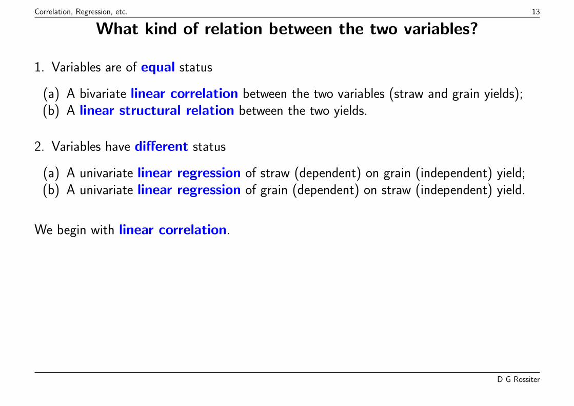
What kind of relation between the two variables?
1. Variables are of equal status
(a) A bivariate linear correlation between the two variables (straw and grain yields);(b) A linear structural relation between the two yields.
2. Variables have different status
(a) A univariate linear regression of straw (dependent) on grain (independent) yield;(b) A univariate linear regression of grain (dependent) on straw (independent) yield.
We begin with linear correlation.
D G Rossiter
Correlation, Regression, etc. 14
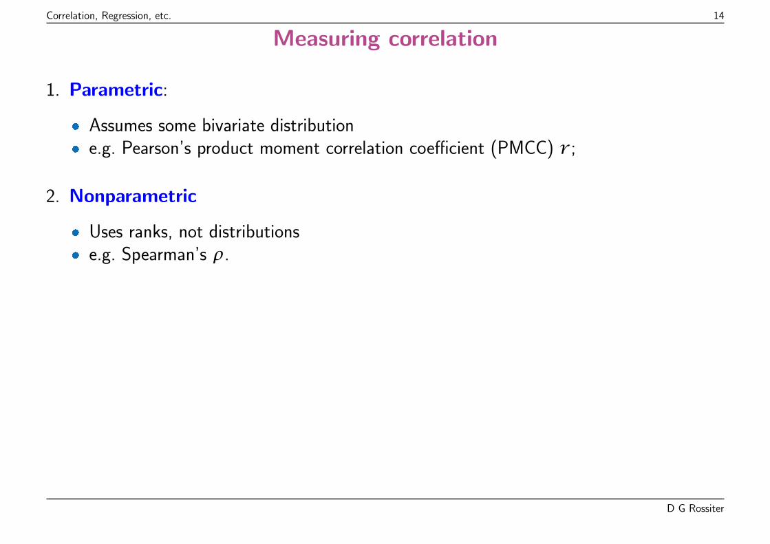
Measuring correlation
1. Parametric:
� Assumes some bivariate distribution� e.g. Pearson’s product moment correlation coefficient (PMCC) r ;
2. Nonparametric
� Uses ranks, not distributions� e.g. Spearman’s ρ.
D G Rossiter
Correlation, Regression, etc. 15
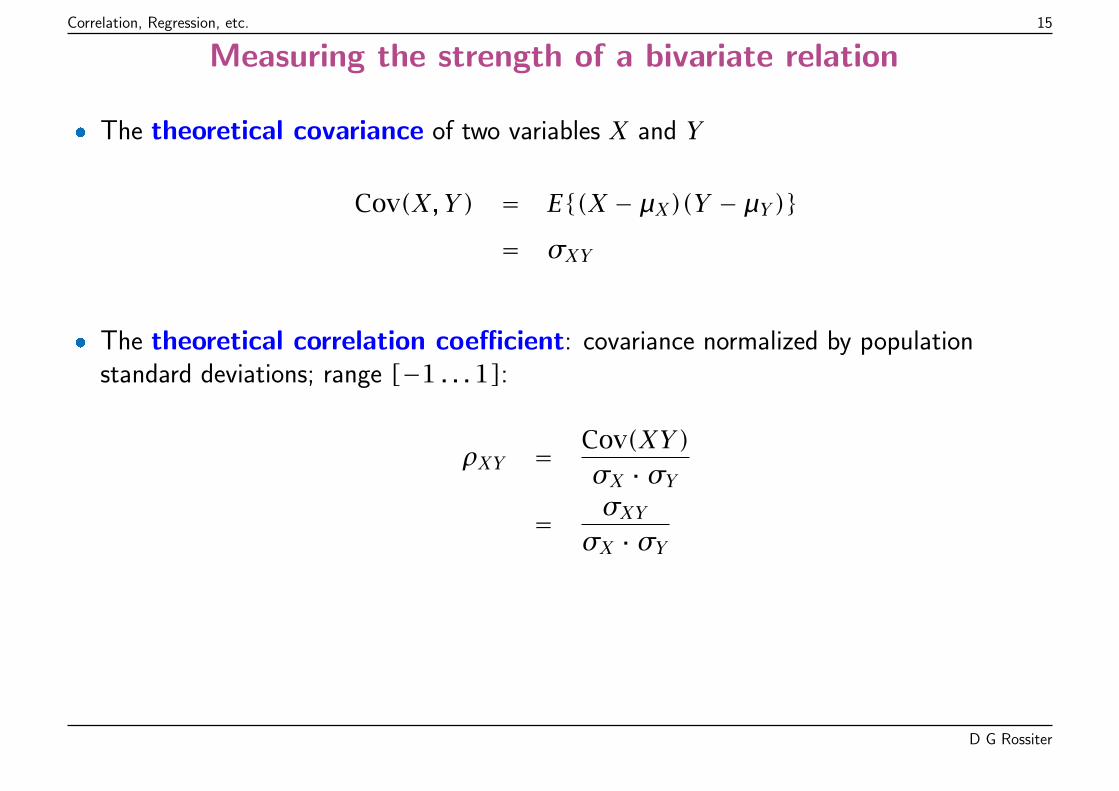
Measuring the strength of a bivariate relation
� The theoretical covariance of two variables X and Y
Cov(X, Y) = E{(X − µX)(Y − µY)}= σXY
� The theoretical correlation coefficient: covariance normalized by populationstandard deviations; range [−1 . . .1]:
ρXY = Cov(XY)σX · σY
= σXYσX · σY
D G Rossiter
Correlation, Regression, etc. 16
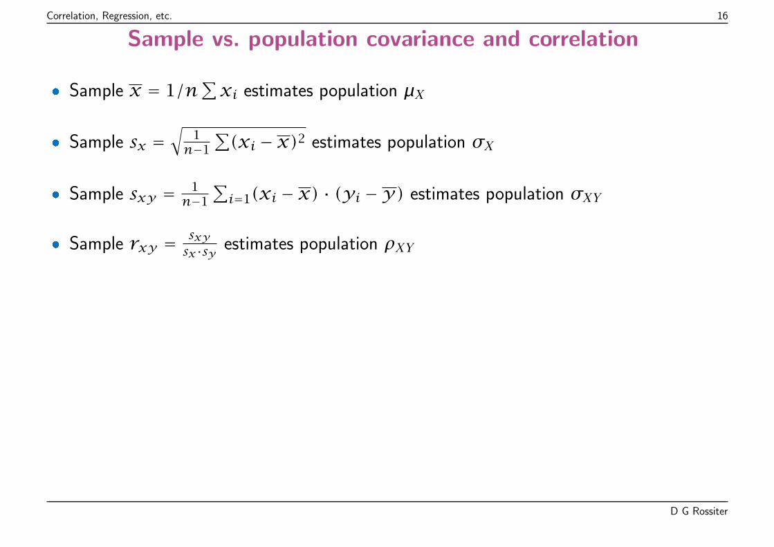
Sample vs. population covariance and correlation
� Sample x = 1/n∑xi estimates population µX
� Sample sx =√
1n−1
∑(xi − x)2 estimates population σX
� Sample sxy = 1n−1
∑i=1(xi − x) · (yi −y) estimates population σXY
� Sample rxy = sxysx·sy estimates population ρXY
D G Rossiter
Correlation, Regression, etc. 17
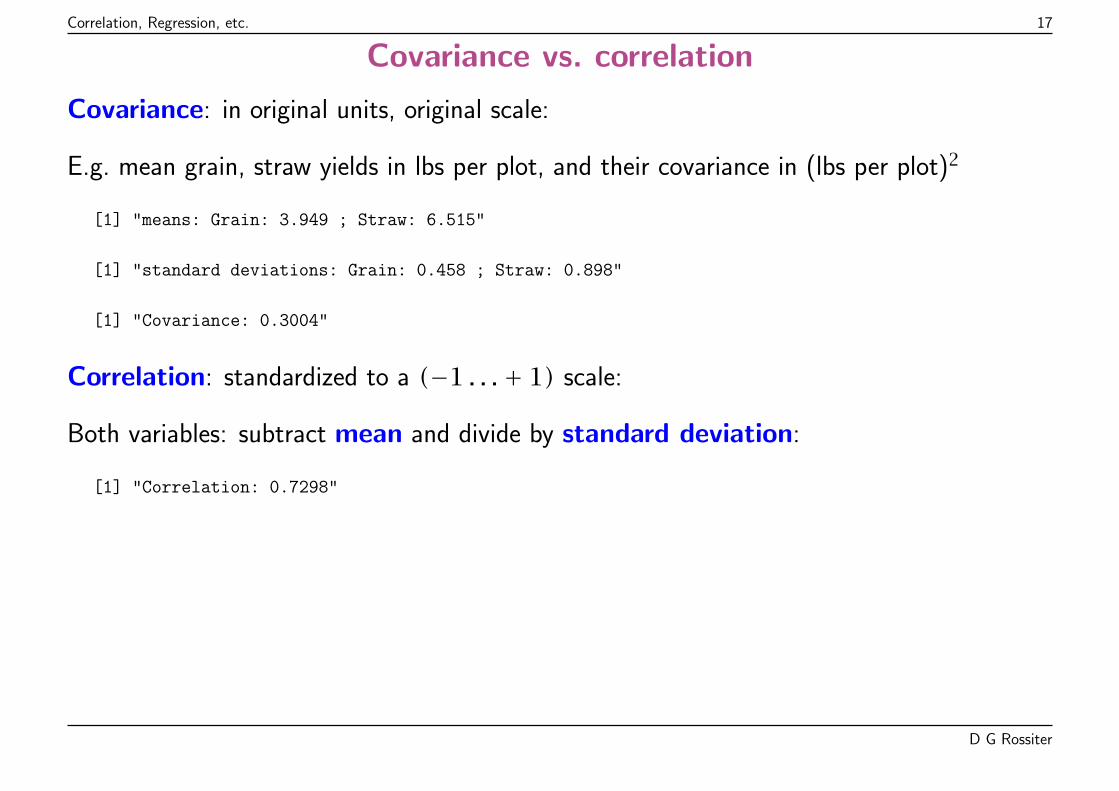
Covariance vs. correlation
Covariance: in original units, original scale:
E.g. mean grain, straw yields in lbs per plot, and their covariance in (lbs per plot)2
[1] "means: Grain: 3.949 ; Straw: 6.515"
[1] "standard deviations: Grain: 0.458 ; Straw: 0.898"
[1] "Covariance: 0.3004"
Correlation: standardized to a (−1 . . .+ 1) scale:
Both variables: subtract mean and divide by standard deviation:
[1] "Correlation: 0.7298"
D G Rossiter
Correlation, Regression, etc. 18
Assumptions for parametric correlation
Requires bivariate normality; do these two variables meet that?
If the assumption isn’t met, must use either:
� transformations to bivariate normality (may be impossible), or
� ranks (see below)
D G Rossiter
Correlation, Regression, etc. 19
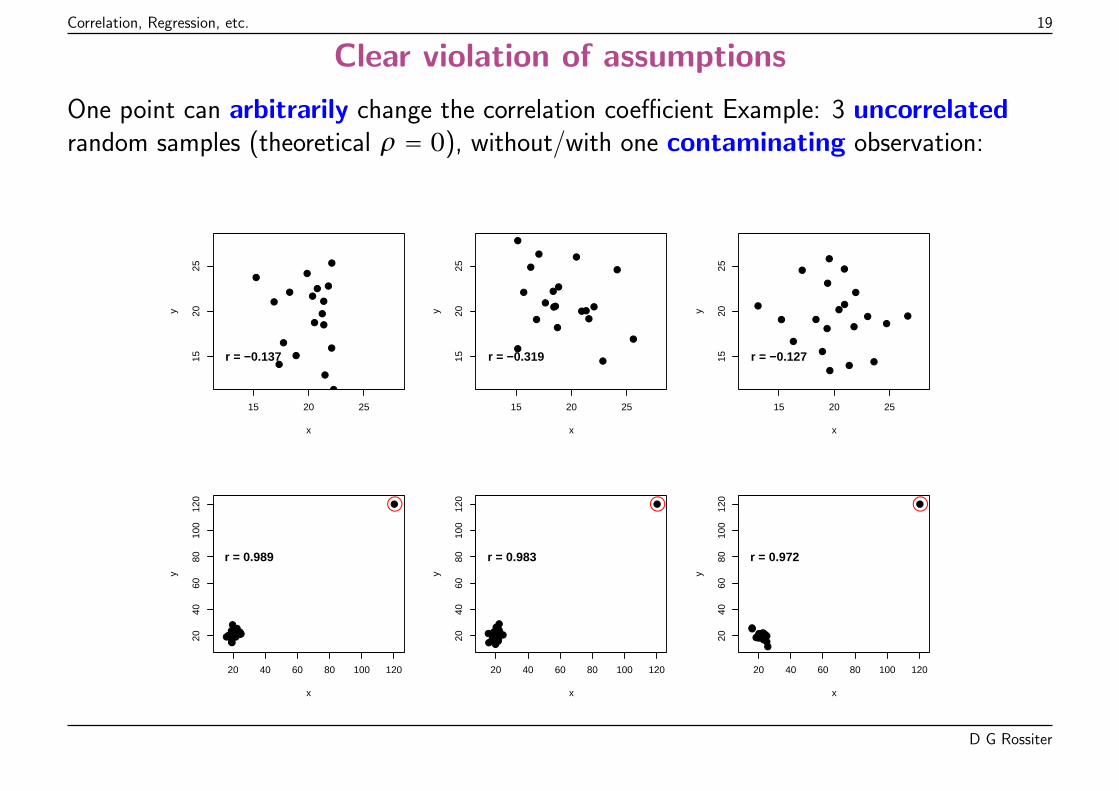
Clear violation of assumptions
One point can arbitrarily change the correlation coefficient Example: 3 uncorrelatedrandom samples (theoretical ρ = 0), without/with one contaminating observation:
●
●
●
●
●
●
●
●
●
●
●
●
●●
●
●
●
●
●
●
15 20 25
1520
25
x
y
r = −0.137
●
●
●
●
●●
●●
●
●
●
●●
●
●
●●
●
●
●
15 20 25
1520
25
xy
r = −0.319●
● ●
●
●
●
●
●
●
●
●
●
●●
●
●
●
●
●●
15 20 25
1520
25
x
y
r = −0.127
●●●●●
●●●
●●●●
●
●●●● ●●
●
20 40 60 80 100 120
2040
6080
100
120
x
y
●
r = 0.989
●●
●●
●
●
●● ●●
●●●●●
●●
●●
●
20 40 60 80 100 120
2040
6080
100
120
x
y
●
r = 0.983
●●●●
●●●●●●●
●●
●
●●●●●
●
20 40 60 80 100 120
2040
6080
100
120
xy
●
r = 0.972
D G Rossiter
Correlation, Regression, etc. 20
Visualizing bivariate normality
To visualize whether a particular sample meets the assumption:
1. Draw random samples that in theory could have been observed from samples of thesame size, if the data are from the theoretical bivariate normal distribution requiredfor PPMC. This is simulating a sample from known (assumed) population.
Note: R functions for simulating samples:
� rnorm (univariate normal);� mvrnorm from the MASS package (multivariate normal)
2. Display them next to the actual sample:
(a) univariate: histograms, Q-Q plots(b) bivariate: scatterplots
They should have the same form.
D G Rossiter
Correlation, Regression, etc. 21
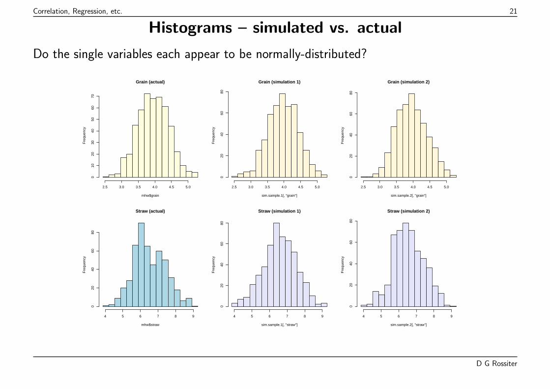
Histograms – simulated vs. actual
Do the single variables each appear to be normally-distributed?
Grain (actual)
mhw$grain
Fre
quen
cy
2.5 3.0 3.5 4.0 4.5 5.0
010
2030
4050
6070
Grain (simulation 1)
sim.sample.1[, "grain"]
Fre
quen
cy
2.5 3.0 3.5 4.0 4.5 5.0
020
4060
80
Grain (simulation 2)
sim.sample.2[, "grain"]
Fre
quen
cy
2.5 3.0 3.5 4.0 4.5 5.0
020
4060
80
Straw (actual)
mhw$straw
Fre
quen
cy
4 5 6 7 8 9
020
4060
80
Straw (simulation 1)
sim.sample.1[, "straw"]
Fre
quen
cy
4 5 6 7 8 9
020
4060
80
Straw (simulation 2)
sim.sample.2[, "straw"]
Fre
quen
cy
4 5 6 7 8 9
020
4060
80
D G Rossiter
Correlation, Regression, etc. 22
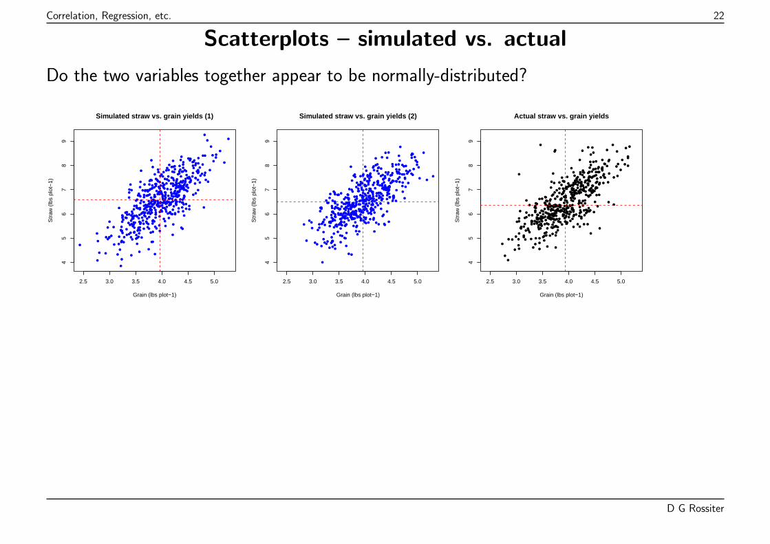
Scatterplots – simulated vs. actual
Do the two variables together appear to be normally-distributed?
●
●
●
●
●
●
●
●
●
●
●
●
●
●
●
●
●
●
●
●
●
●
●●
●
●
●
●
●
●
●
●
●
●
●
●
●
●
●
●
●
●
●
●
●
●●
●
●
●
●
●
●
●
●
●
●
●
●
●
●
●
●
●
●
●
●
●
●
●
●
●
●
●
●
●
●
●
●
●
●
●
●
●
●
●
●
●
●
●
●
●
●
●
●
●
●
●
●
●
●
●
●
●●
●
●
●
●
●
●
●
●
●
●
●
●
●
●
●
●
●
●
●
●
●
●
●
●
●
●
●
●●
●
●
●
●
●
●
●
●
●
●
●
●
●
●
●●
●
●
●
●
●
●
●
●●
●
●
●
●
●
●
●
●
●●
●
●
●
●
●
●
●
●
●
●
●
●
●
●
●
●
●
●
●
●
●
●
●
●
●
●
●
●
●
●
●
●
●
●
●
●
●
●
●
●
●
●
●
●
●
●
●
●●
●
●
●
●
●
●●
●
●
●
●
●
●
●
●
●
●
●
●
●
●
●
●
●
●
●
●
●
●
●
●
●
●
●
●
●
●
●
●
●
●
●
●
●
●
●
●
●
●●
●
●
●
●
●●
●
●
●
●
●
●
●
●
●
●
●
●
●
●
●
●●
●
●
●
●
●
●
●
●
●
●
●
●
●
●
●
●
●
●
●
●
●
●
●
●●
● ●
●
●
●
●
●
●
●
●
●
●
●
●
●●
●
●
●
●●
●
●
●
●
●
●
●
●
●
●
●
●
●
●
●
●
●
●
●
●
●
●
●
●
●
●
●
●●
●
●
●
●
●
●
●
●
●
●
●
●
●
●
●
●
●
●
●
●
●
●
●
●
●
●
●
●
●
●
●
●
●
●
●
●
●
●
●
●
●
●
●
●
●
●●
●
●
●
●
●
●
●
●
●
●
●
●
●
●
●
● ●
●
●
●
●
●
●
●
●
●
●
●
●
●
●●
●
●
●
●
●
●
●
●
●
●
●
●●
●
●
●
●
●
●
●
●
●
●
●
●
●●
●
●●
●
●
● ●●
●
●
●
●
●
●
●
●
●
●
●
●
●
●
●
●
●
●
●
●
2.5 3.0 3.5 4.0 4.5 5.0
45
67
89
Simulated straw vs. grain yields (1)
Grain (lbs plot−1)
Str
aw (
lbs
plot
−1)
●
●
●
●
●
●
●
●
●
●
●
●
●
●
●
●
●
●
●
●
●
●
●
●
●
●
●
●
●
●
●
●
● ●●
●
●
●
●
●
●●
●
●
●●
●
●
●
●
●●
●
●
●
●
●
●
●
● ●
●
●
●
●
●
●
●
●
●
●
●
●
●
●
●
●
●
●
●
●
●●
●
●
●●
●
●
●
●
●
● ●
●● ●
●
●
●
●
●
●
●
●
●
●
●
●
●●
●●
●
●
●
●
●
●
●
●
●
●●
●
●
●
●
●
●
●
●
●
●
●
●
●
●
●
●
●
●●
●
●
●
●
●
●
●
●
●
●
●
●
●
●
●
●
●
●
●
●
●
●
●●
●
●●
●
●
●●
●
●
●
●
● ●
●
●
●
●
●
●
●
●
●
●
●
●
●
●
●
●
●
●
●
●
●
● ●
●●
●●
●
●
●
●
●
●
●
●
●
●
●
●
●
●
●
●
●
●
●
●
●
●
●
●
●
●
●
●
●
●
●
●
●
●
●
●●
●
●
●
●
●
●
●
●
●
●
●
●
●
●
●
●
●
●
●
●
●
●●
●
●
●
●
●
●●
●
●
●
●
●
●
●
●
●
●
●
●
●
●
●
●
●
●
●
●
●
●
●
●
●
●
●
●
●
●●
●
●
●
●
●●
●
●
●
●
●
●
●
●
●
●
●
●
●
●
●
●
●
●
●
●
●
●
●
● ●
●
●
●
●
●
●
●
●
●
●
●
●
●
●
●
●
●
●
●
●
●
●●
●
●
●
●
●
●
●
●
●
●
●
●
●
●
●
●
●
●
●
●
●
●
●
● ●
●●
●
●
●
●
●
●
●
●●
●
●
●
●
●
●●●
●
●
●
●
●
●
●
●
●
●
●
●
●
●
●
●
●
●
●●
●
●
●
●
●
●
●
●
●
●
●
●
●
●
●
●
●
●
●
●
●
●●
●
●
●
●
●
●
●
●
●●
●
●●
●
●
●
●
●
●
●
●
●
●
●
●
●
●
●
●
●
●
●
●
●
●●
●●●
●
●
●
●
●
●
●
●
●
●
●
●
●
●●
2.5 3.0 3.5 4.0 4.5 5.0
45
67
89
Simulated straw vs. grain yields (2)
Grain (lbs plot−1)
Str
aw (
lbs
plot
−1)
●
●
●
●
●
●
●
●
●
●●
● ●●
●
●
●
●
●
●
●
●
●
●
●
●
●
●
●
●●
●
●
●
●
●
●
●
●
●
●
●●
●
●
● ●●
●
●
●
●
●
●
●
●
●
●
●
●
●
●
●
●
●
●
●
●
●●
●
●
●
●
●
●
●
●
●●
●
●
●
●
●
●
●
●
●
●
●
●
● ●
●
●
●
●
●
●
●
●
●
●
●
●● ●
● ●
●
●
●
●
●
●
●
●
●
●
●
●
●
●
●
●
●
●
●
●
●
●
●
●
●
●
●●
●
●
●
●
●
●●
●
●
●
●
●
●●
●●
●
●
●
●
●
●
●●
●
●
●
●
●
●
●●
●
●●
●
●
●
●
●
●●
●
●
●
●
●
●
●●
●
●● ●●
●
●
●
●
●
●
●
●
●●
●
●
●
●●
●
●
●
●
●
●
●
●
●
●
●
●
●
●●
●
●
●
●
●
●
●
●
●
●
●
●
●
●
●
●
●
●
●
●
●●
●
●
●
●
●
●
●
●
●
●
●
●
●
●
●
●
●
●
●
●
●●
●
●
●●
●
● ●
●
●
●
●
●
●
●
●
●
●
●
●
●
●
●
●
●●
●
●
●
●
●
●
●
● ●
●
●
●
●
●
●
●
●
●
●
●
●
●
●
●
●
●
●●
●
●
●
●
●
●
●
●
●
●
●
●
●
●
●
●
●
●
●
●
●
●
●
●
●
●
●
●
●●●
●
●●
●
●
●
●
●
●
●
●
●
●
●
●
●
●
●
●
●
●
●
●
●●
● ●
●
●
●
●
●
●
●
●
●
●
●●
●
●
●
●
● ●●
●
●
●
●
●
●●
● ●
●
●
●
●
●
●
●
● ●
●
●●
●
●
●
●
●
●
●
●
●
●
●●
●●
●
●
●
●
●
● ●
●
●
●
●
●
●
●
●
●
●●
●
●
●
●
●
●
●●
●
●
●
●
●
●
●●
●
●
●
●
●
●
●●●
●
●
●
●
●
●
●
●
● ●
●
●
●
●
●
●
●
●
●
●
●
●
●
●
●
2.5 3.0 3.5 4.0 4.5 5.0
45
67
89
Actual straw vs. grain yields
Grain (lbs plot−1)
Str
aw (
lbs
plot
−1)
D G Rossiter
Correlation, Regression, etc. 23
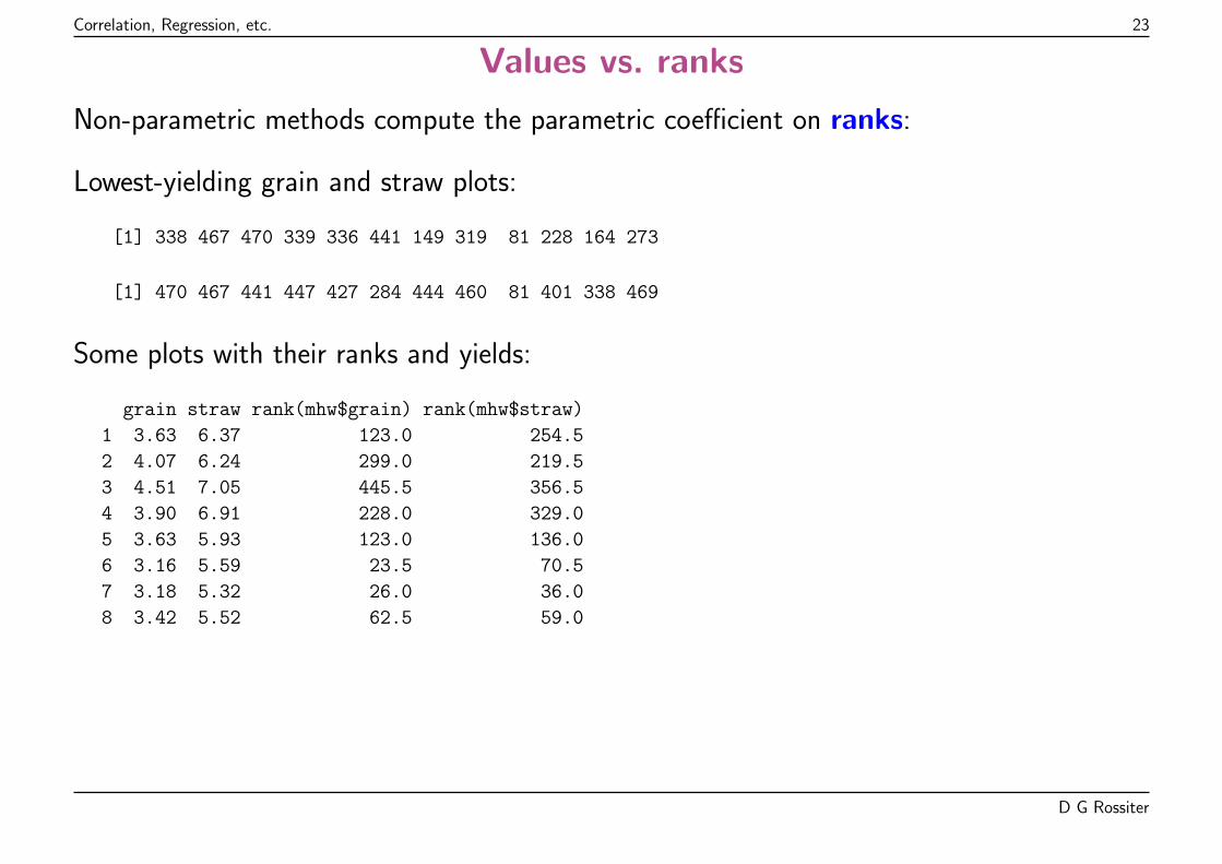
Values vs. ranks
Non-parametric methods compute the parametric coefficient on ranks:
Lowest-yielding grain and straw plots:
[1] 338 467 470 339 336 441 149 319 81 228 164 273
[1] 470 467 441 447 427 284 444 460 81 401 338 469
Some plots with their ranks and yields:
grain straw rank(mhw$grain) rank(mhw$straw)
1 3.63 6.37 123.0 254.5
2 4.07 6.24 299.0 219.5
3 4.51 7.05 445.5 356.5
4 3.90 6.91 228.0 329.0
5 3.63 5.93 123.0 136.0
6 3.16 5.59 23.5 70.5
7 3.18 5.32 26.0 36.0
8 3.42 5.52 62.5 59.0
D G Rossiter
Correlation, Regression, etc. 24
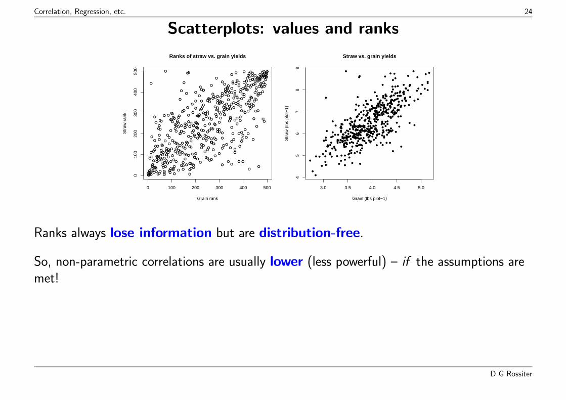
Scatterplots: values and ranks
●
●
●
●
●
●
●
●
●
●●
● ●●
●●
●
●
●
●
●
●
●
●
●
●
●
●
●
●●
●
●
●
●
●
●
●
●
●
●
●●
●
●
● ●●
●
●
●
●
●
●
●
●
●
●
●●
●●
●
●
●●
●
●
●●
●
●
●
●
●
●
●
●
●●
●
●
●
●
●
●
●
●
●
●
●
●
● ●
●
●
●
●
●
●
●
●
●
●
●
●
●●
● ●
●●
●●
●
●
●●
●
●
●
●●
●
●
●
●
●
●
●
●●
●
●
●
●
●●
●
●
●
●
●
●●
●
●
●
●
●
●●
●●
●
●
●
●
●
●
●●
●
●
●
●
●
●
●●
●
●●
●
●
●
●
●
●●
●
●
●
●
●
●
●●
●
●● ●●
●
●
●
●
●
●
●
●
●
●
●
●
●
●
●
●
●
●
●
●
●
●
●
●
●
●
●
●
●●
●
●
●
●
●
●
●
●
●
●
●
●
●
●
●
●●
●
●
●
●
●
●
●
●
●
●
●
●
●
●
●
●
●
●
●
●
●
●
●
●
●
●●
●
●
●●
●
● ●
●
●
●
●
●
●
●
●
●
●
●
●
●
●
●
●
● ●
●
●
●
●
●
●
●
● ●
●
●
●
●
●
●
●
●
●
●
●
●
●
●
●
●
●
●●
●●
●
●
●
●
●
●
●
●
●
●
●
●
●
●
●
●●
●
●
●
●
●
●
●
●
●
●
●●
●
●
●
●
●
●
●
●
●
●
●
●
●
●
●
●
●
●
●
●
●
●
●
● ●
● ●
●
●
●
●
●
●
●
●
●
●
●
●
●
●
●
●
● ●●
●
●
●
●
●
●
●
● ●
●
●
●
●
●
●
●
● ●
●
●●
●
●
●●
●
●
●
●
●
●
●●
●●
●
●
●
●
●
●●
●
●
●
●
●
●
●
●
●
●●
●
●
●
●
●
●
●●
●
●
●
●
●
●
●●
●
●
●●
●
●
●●
●
●
●
●
●
●
●
●
●
● ●
●
●
●
●
●
●
●
●
●
●
●
●
●
●
●
0 100 200 300 400 500
010
020
030
040
050
0
Ranks of straw vs. grain yields
Grain rank
Str
aw r
ank
●
●
●
●
●
●
●
●
●
●●
● ●●
●
●
●
●
●
●
●
●
●
●
●
●
●
●
●
●●
●
●
●
●
●
●
●
●
●
●
●●
●
●
● ●●
●
●
●
●
●
●
●
●
●
●
●
●
●
●
●
●
●
●
●
●
●●
●
●
●
●
●
●
●
●
●●
●
●
●
●
●
●
●
●
●
●
●
●
● ●
●
●
●
●
●
●
●
●
●
●
●
●● ●
● ●
●
●
●
●
●
●
●
●
●
●
●
●
●
●
●
●
●
●
●
●
●
●
●
●
●
●
●●
●
●
●
●
●
●●
●
●
●
●
●
●●
●●
●
●
●
●
●
●
●●
●
●
●
●
●
●
●●
●
●●
●
●
●
●
●
●
●
●
●
●
●
●
●
●●
●
●● ●●
●
●
●
●
●
●
●
●
●●
●
●
●
●●
●
●
●
●
●
●
●
●
●
●
●
●
●
●●
●
●
●
●
●
●
●
●
●
●
●
●
●
●
●
●
●
●
●
●
●●
●
●
●
●
●
●
●
●
●
●
●
●
●
●
●
●
●
●
●
●
●●
●
●
●●
●
● ●
●
●
●
●
●
●
●
●
●
●
●
●
●
●
●
●
●●
●
●
●
●
●
●
●
● ●
●
●
●
●
●
●
●
●
●
●
●
●
●
●
●
●
●
●●
●
●
●
●
●
●
●
●
●
●
●
●
●
●
●
●
●
●
●
●
●
●
●
●
●
●
●
●
●
●●
●
●●
●
●
●
●
●
●
●
●
●
●
●
●
●
●
●
●
●
●
●
●
●●
● ●
●
●
●
●
●
●
●
●
●
●
●●
●
●
●
●
● ●●
●
●
●
●
●
●●
● ●
●
●
●
●
●
●
●
● ●
●
●●
●
●
●
●
●
●
●
●
●
●
●●
●●
●
●
●
●
●
● ●
●
●
●
●
●
●
●
●
●
●●
●
●
●
●
●
●
●●
●
●
●
●
●
●
●●
●
●
●
●
●
●
●●●
●
●
●
●
●
●
●
●
● ●
●
●
●
●
●
●
●
●
●
●
●
●
●
●
●
3.0 3.5 4.0 4.5 5.0
45
67
89
Straw vs. grain yields
Grain (lbs plot−1)
Str
aw (
lbs
plot
−1)
Ranks always lose information but are distribution-free.
So, non-parametric correlations are usually lower (less powerful) – if the assumptions aremet!
D G Rossiter
Correlation, Regression, etc. 25
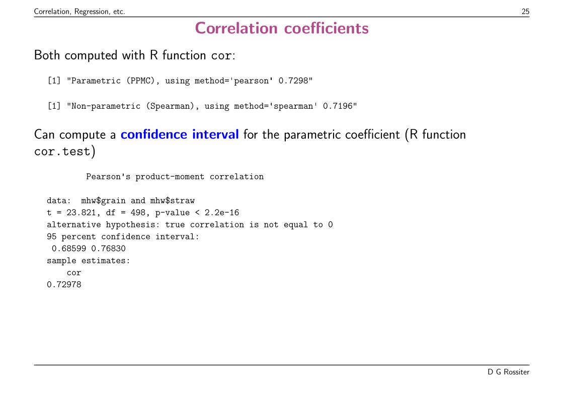
Correlation coefficients
Both computed with R function cor:
[1] "Parametric (PPMC), using method='pearson' 0.7298"
[1] "Non-parametric (Spearman), using method='spearman' 0.7196"
Can compute a confidence interval for the parametric coefficient (R functioncor.test)
Pearson's product-moment correlation
data: mhw$grain and mhw$straw
t = 23.821, df = 498, p-value < 2.2e-16
alternative hypothesis: true correlation is not equal to 0
95 percent confidence interval:
0.68599 0.76830
sample estimates:
cor
0.72978
D G Rossiter
Correlation, Regression, etc. 26
Topic: Simple Linear Regression
Recall: regression is a general term for modelling one or more:
� response variables (predictands), from one or more
� predictor variables
The simplest case is simple linear regression:
1. One continous predictor
2. One continous predictand
D G Rossiter
Correlation, Regression, etc. 27
Fixed effects model
Yi = BXi + εi
All error ε is associated with the predictand Yi
There is no error in the predictors Xi, either because:
� imposed by researcher without appreciable error (e.g. treatments);
� measured without appreciable error;
� ignored to get “best” prediction of Y .
The coefficients B are chosen to minimize the error in the predictand Y .
Simplest case: a line: slope β1, intercept β0:
yi = β0 + β1xi + εi
D G Rossiter
Correlation, Regression, etc. 28
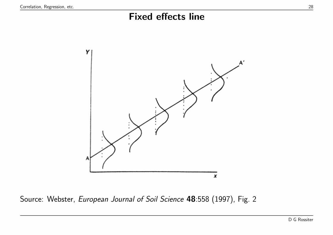
Fixed effects line
Source: Webster, European Journal of Soil Science 48:558 (1997), Fig. 2
D G Rossiter
Correlation, Regression, etc. 29
Least-squares solution
Two parameters must be estimated from the data:
The slope βY .x is estimated from the sample covariance sXY and variances of thepredictand s2
x:
� βY .x = sXY/s2x
The intercept αY .x is then adjusted to make the line go through the centroid (x, y):
� αY .x = y − βY .xx
Note: only s2x is used to compute the slope! It is a one-way relation, because all the error
is assumed to be in the predictand.
This is the simplest case of the orthogonal projection (see below).
This solution has some strong assumptions, see below.
D G Rossiter
Correlation, Regression, etc. 30
Matrix formulation
The general form of the linear model is Y = XB + ε; if there is only one response variable,this is y = Xb + ε.
X is called the design matrix, with one column per predictor, with that predictor’s valuefor the observation i.
In the simple linear regression case, there is only one predictor variable x, and the designmatrix X has an inital column of 1’s (representing the mean) and a second column of thepredictor variable’s values at each observation:
y1
y2
. . .yn
=
1 x1
1 x2
. . .1 xn
[b0
b1
]+
ε1
ε2
. . .εn
where the ε are identically and indepenently distributed (IID).
D G Rossiter
Correlation, Regression, etc. 31
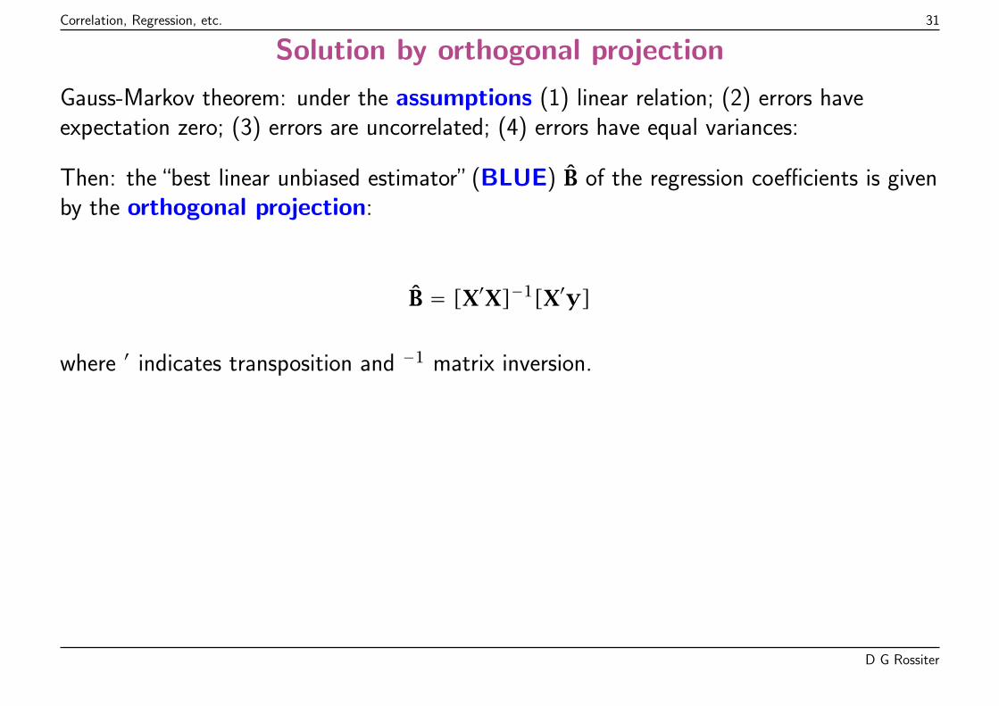
Solution by orthogonal projection
Gauss-Markov theorem: under the assumptions (1) linear relation; (2) errors haveexpectation zero; (3) errors are uncorrelated; (4) errors have equal variances:
Then: the “best linear unbiased estimator” (BLUE) B of the regression coefficients is givenby the orthogonal projection:
B = [X′X]−1[X′y]
where ′ indicates transposition and −1 matrix inversion.
D G Rossiter
Correlation, Regression, etc. 32
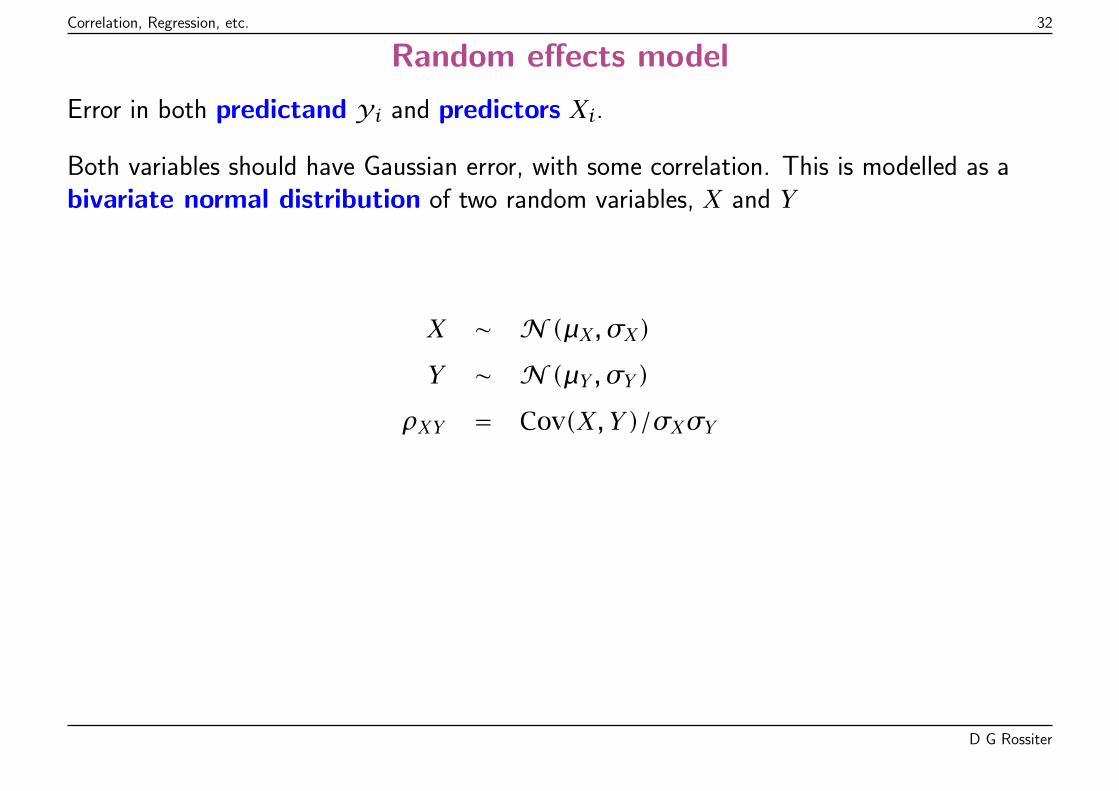
Random effects model
Error in both predictand yi and predictors Xi.
Both variables should have Gaussian error, with some correlation. This is modelled as abivariate normal distribution of two random variables, X and Y
X ∼ N (µX, σX)Y ∼ N (µY , σY)
ρXY = Cov(X, Y)/σXσY
D G Rossiter
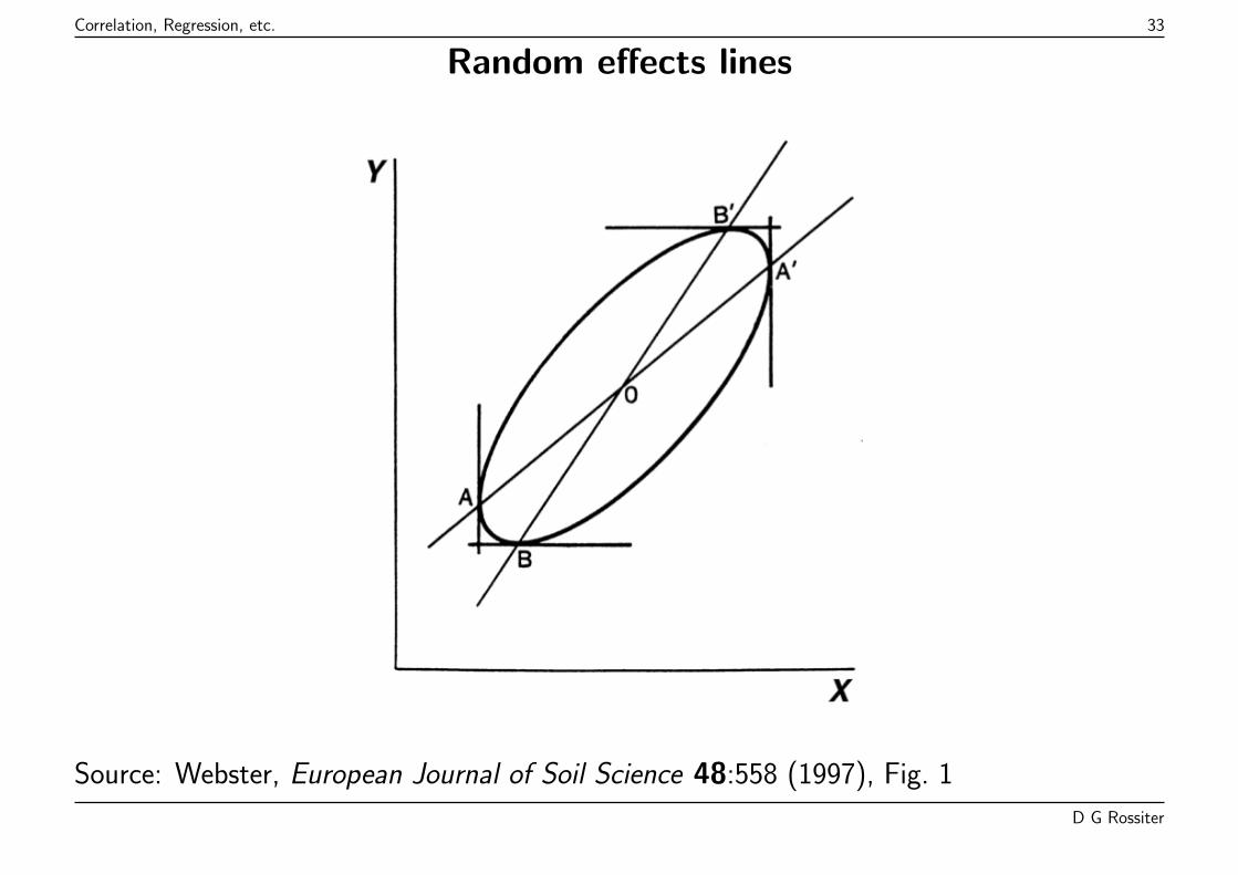
Correlation, Regression, etc. 33
Random effects lines
Source: Webster, European Journal of Soil Science 48:558 (1997), Fig. 1
D G Rossiter
Correlation, Regression, etc. 34
Fitting a regression line
Fit a line that “best” describes the response-predictor relation.
Different levels of assumptions about functional form:
1. Exploratory, non-parametric
2. Parametric
3. Robust
D G Rossiter
Correlation, Regression, etc. 35
A parametric linear fit
Model straw yield as function of grain yield, by minimizing the sum-of-squares of theresiduals (Gaussian least-squares).
Although there is error in both the grain and straw yield (random effects model), the aimis to minimize error in the predictand.
This is because the model is used to explain the predictand in terms of the predictor, andeventually to predict in that direction.
Once one variable is selected as the response, then the aim is to minimize that error, andthe one-way least-squares fit is applied.
D G Rossiter
Correlation, Regression, etc. 36
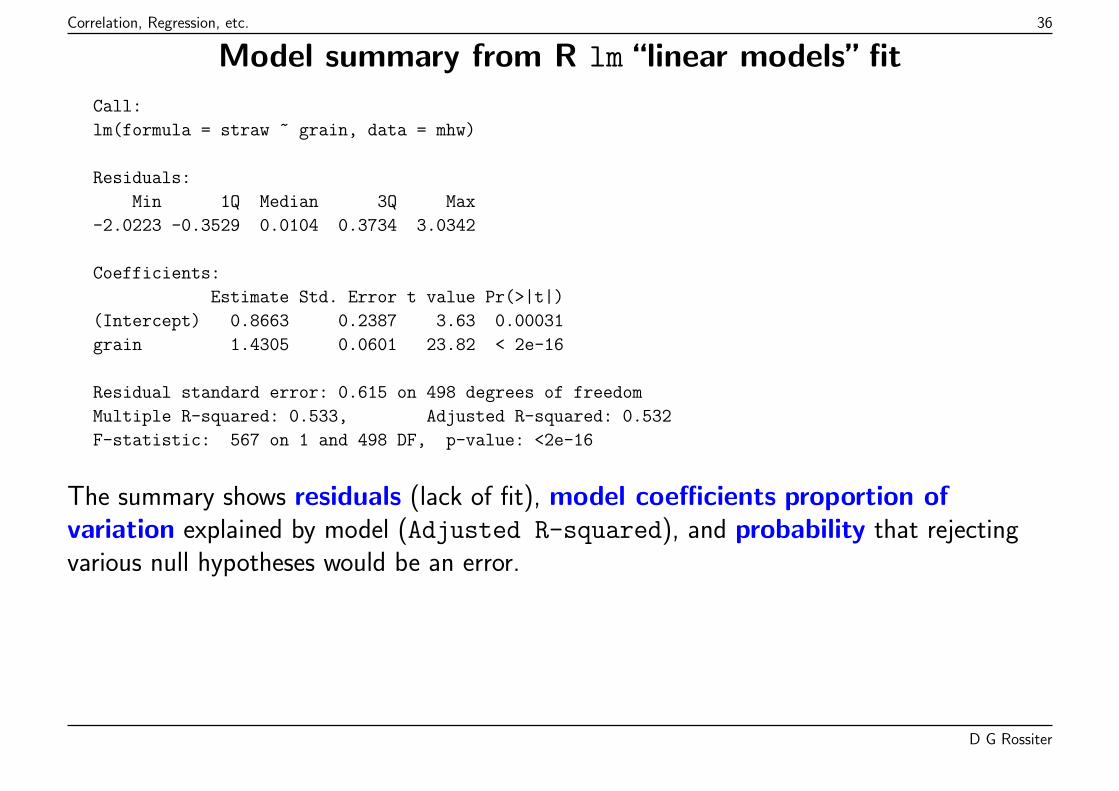
Model summary from R lm“linear models” fit
Call:
lm(formula = straw ~ grain, data = mhw)
Residuals:
Min 1Q Median 3Q Max
-2.0223 -0.3529 0.0104 0.3734 3.0342
Coefficients:
Estimate Std. Error t value Pr(>|t|)
(Intercept) 0.8663 0.2387 3.63 0.00031
grain 1.4305 0.0601 23.82 < 2e-16
Residual standard error: 0.615 on 498 degrees of freedom
Multiple R-squared: 0.533, Adjusted R-squared: 0.532
F-statistic: 567 on 1 and 498 DF, p-value: <2e-16
The summary shows residuals (lack of fit), model coefficients proportion ofvariation explained by model (Adjusted R-squared), and probability that rejectingvarious null hypotheses would be an error.
D G Rossiter
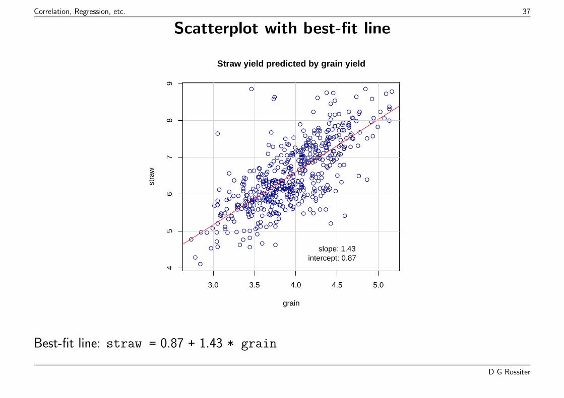
Correlation, Regression, etc. 37
Scatterplot with best-fit line
●●
●●
●
●
●
●
●
●●
● ●●
●
●
●
●●
●
●
●
●
●
●
●
●
●
●
●●●
●
●
●
●
●
●
●
●
●
● ●
●
●
● ●●
●
●
●
●
●
●
●
●●
●
●
●
●
●
●
●
●●
●
●
●●
●
●
●
●
●
●
●
●
●●
●
●
●
●
●
●
●
●
●
●●
●
● ●
●
●
●
●
●
●
●
●
●
●
●
●● ●
● ●
●
●
●
●
●
●
●●
●
●
●
●
●
●
●
●
●
●
●
●
●
●
●
●
●
●
●●
●
●
●
●
●
●●
●
●
●
●
●
● ●
●●
●
●
●
●●
●
●●
●●
●
●
●
●
●●
●
●●
●
●
●
●
●
●●
●
●
●
●
●
●
● ●
●
●● ● ●
●
●
●
●
●
●
●
●
●●
●
●
●
●●
●
●
●
●
●
●
●
●
●
●
●
●
●
●●
●
●
●
●
●
●
●
●
●
●
●
●
●
●
●
●●
●
●
●
●●●
●
●
●
●
●●
●
●●
●
●
●
●●
●
●
●
●
●
●●
●
●
●●
●
● ●
●
●
●
●
●
●
●
●
●
●
●
●
●●
●
●
● ●
●
●
●
●
●
●
●
● ●
●
●
●
●●
●
●
●
●
●
●
●
●
●
●
●
●
●●
●●
●
●
●
●
●
●
●
●
●
●
●
●
●
●
●
●
●
●
●
●
●
●
●
●●
●
●●●
●
●●
●
●
●
●
●
●
●
●
●
●
●
●
●
●
●
●
●
●
●●
● ●
● ●
●
●
●
●
●
●
●●
●
●
●●
●
●
●
●
● ●●
●●
●
●
●
●●
● ●
●
●●
●
●
●
●
● ●
●
●●
●
●
●●
●
●
●
●
●
●●
●
●●
●●
●
●
●
● ●●
●
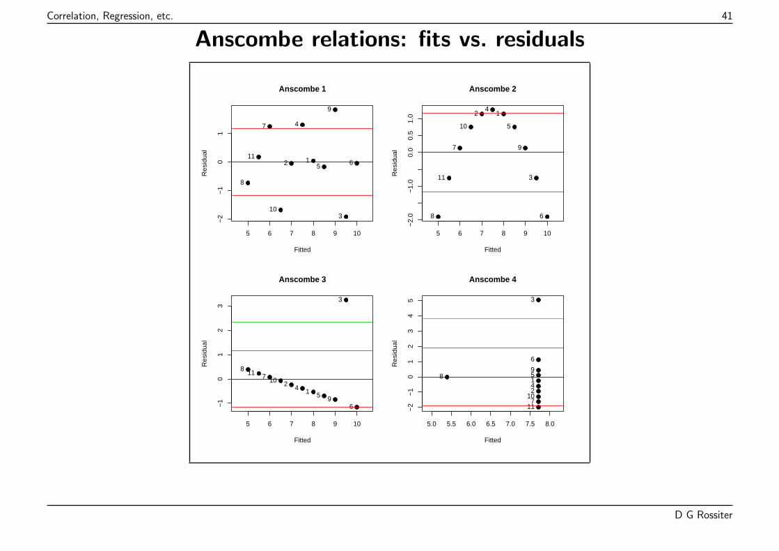
●
●
●
●
●
●
●
●●
●
●
●
●
●
●
●●
●
●
●
●
●
●
●●
●
●
●
●
●
●
●●●
●
●
●
●
●
●
●
●
● ●
●
●
●
●
●
●
●
●
●
●
●
●
●
●
●
3.0 3.5 4.0 4.5 5.0
45
67
89
grain
stra
w
Straw yield predicted by grain yield
slope: 1.43intercept: 0.87
Best-fit line: straw = 0.87 + 1.43 * grain
D G Rossiter
Correlation, Regression, etc. 38
Assumptions of the linear model
The least-squares (parametric) solution is only valid under a strong assumption:
The residuals are identically and indepenently distributed (IID) from a normaldistribution
This implies:
1. no dependence of residual on fitted values;
2. no difference in spread of residuals through fitted value range: homoscedascity
3. residuals have a normal distribution (µε ≡ 0)
D G Rossiter
Correlation, Regression, etc. 39
Model diagnostics
The assumptions can visualized and tested.
The most important tools are the diagnostic plots.
These are of several kinds; the most important are:
� Normal probability plot of the residuals
� Plot of residuals vs. fits
� Leverage of each observation (influence on fit)
� Cook’s distance to find poorly-fitted observations
D G Rossiter
Correlation, Regression, etc. 40
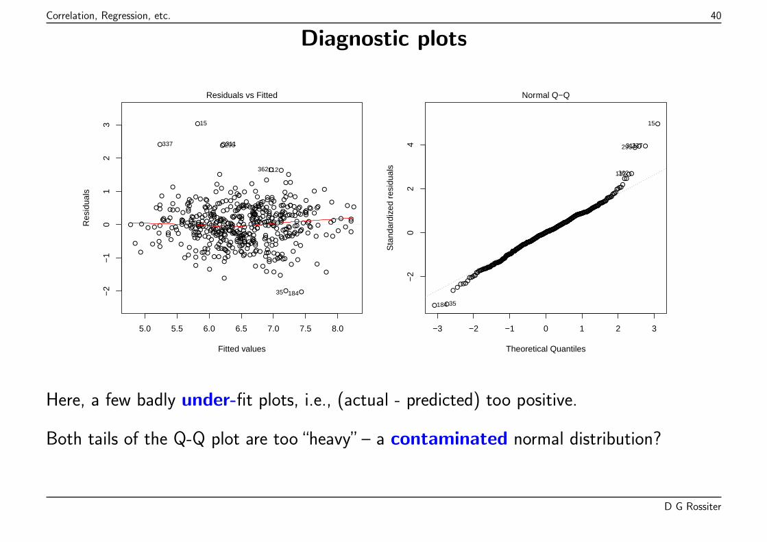
Diagnostic plots
5.0 5.5 6.0 6.5 7.0 7.5 8.0
−2
−1
01
23
Fitted values
Res
idua
ls
●
●●
●
●
●
●●
●
●● ●●
●
●
●
●
●
●●●
●
● ●●
●
●● ●●
●
● ●
●
●
●
●
●
●
●
●●
●
●
●
●
●
●
●●●
●
●
●●
●
●●
●
●
●
●
●●
● ●
●●
●●
●
●
●
●
●●
●●
●●
●
●
●● ●●
●●●
●●● ●
●●
●●
●
●
●
●
●
●
● ●●●
●
●●
●
●
●
●
●●
●
●
●●
●
● ●
●
●
●●
●●
●
●
●
●
●●
●●
●
●
●
● ●
●
●
●
●
●●
●
●
●●
●
● ●
●
●●
●
●
●●
●
●
●
●
●●●
● ●
●
●●●
● ●●●
●
●●
●
●
●
●
● ●
●
●●
●
●
●● ●
●●
●
●●●
●
●
●
●
●●● ●
●
●
●
●●● ●
●●
●●
●●
●
●
●
●
●
●
●
●
● ●
●
●
●
●●
●
●
●●
●
●
●●●●
●
● ●●
●
●●
●
●
●
●
●
●
●
●
●
●●●
●
●●
●
●
●
●
●
●
●
●
●
●
●
●
●
●
●
●●●
●
●
●
●
●●
●
● ●
●
●
●
●
●
●
●●
●
●
●
●
●
●
●●
●
●
●●
●
●
●
●●
●
●
●●
●
●
●●
●●
●
●
●
●
●
● ●
●
●
●
●
●
●
●●
●
●●
●
●
●●●
●●
●
●
●
●
●
●
●
●
●
●●
●
●
●●
●●●
●
●
● ●
●
●
●
●●
●● ●
●
●
●
●
●
●
●●
●●
●
●
●
●
●
●
●●
●
●
●
●
● ●●
●
●
●●
●
●
●●
●
●
●
●● ●● ●
●
●
●●
●
●
●
●
●
●
●
●
●
●
●
●
●
●●
●
●
●
●
●
●
●●
●
●
●
●
●
●●
●●
●
●●
●
●●
●
●
●
●●
●●●
●●
●
●
●●
●
●
●
●
●
●
●●
●
●
● ●
●●●
●
Residuals vs Fitted
15
311337 295
18435
362112
●
●
●
●
●
●
●●
●
●●●●
●
●
●
●
●
●●●
●
●●●
●
● ●●
●●
●●
●
●
●
●
●
●
●
●●
●
●
●
●
●
●
●●●
●
●
●●
●
●
●●
●
●
●
●●
●●
●●
●●
●
●
●
●
●●
●●
●●
●
●
●●●●
●
●●
●●●●
●●
●
●
●
●
●
●
●
●
●●●●
●
●●
●
●
●
●
●●
●
●
●●
●
●●
●
●
●●
●●
●
●
●
●
●●
●●
●
●
●
●●
●
●
●
●
●●
●
●
●●
●
●●
●
●●
●
●
●●
●
●
●
●
●●●
●●
●
●●●
●●●●
●
●●
●
●
●
●
●●
●
● ●
●
●
●● ●
●●
●
●●●
●
●
●
●
●●●●
●
●
●
●●●●
●●
●●
●●
●
●
●
●
●
●
●
●
●●
●
●
●
●●
●
●
●●
●
●
●●
●●
●
●●●
●
●●
●
●
●
●
●
●
●
●
●
●●●
●
●●
●
●
●
●
●
●
●
●
●
●
●
●
●
●
●
●●
●
●
●
●
●
●●
●
●●
●
●
●
●
●
●
●●
●
●
●
●
●
●
●●
●
●
●●
●
●
●
● ●
●
●
●●
●
●
●●
●
●●
●
●
●
●
●●
●
●
●
●
●
●
●●
●
●●
●
●
●●●
●●
●
●
●
●
●
●
●
●
●
●●
●
●
●●
●●
●
●
●
●●
●
●
●
●
●
●●●
●
●
●
●
●
●
●●
●●
●
●
●
●
●
●
●●
●
●
●
●
●●●
●
●
●
●
●
●
●●
●
●
●
●●●●●
●
●
●●
●
●
●
●
●
●
●
●
●
●
●
●
●
●●
●
●
●
●
●
●
●●
●
●
●
●
●
●●
●●
●
●●
●
●●
●
●
●
●●
●●●
●●
●
●
●●
●
●
●
●
●
●
●●
●
●
●●
●●●
●
−3 −2 −1 0 1 2 3
−2
02
4
Theoretical Quantiles
Sta
ndar
dize
d re
sidu
als
Normal Q−Q
15
337311295
184 35
362112
Here, a few badly under-fit plots, i.e., (actual - predicted) too positive.
Both tails of the Q-Q plot are too “heavy” – a contaminated normal distribution?
D G Rossiter
Correlation, Regression, etc. 41
Anscombe relations: fits vs. residuals
5 6 7 8 9 10
−2
−1
01
Anscombe 1
Fitted
Res
idua
l
12
3
4
5 6
7
8
9
10
11
5 6 7 8 9 10
−2.
0−
1.0
0.0
0.5
1.0
Anscombe 2
Fitted
Res
idua
l
12
3
4
5
6
7
8
9
10
11
5 6 7 8 9 10
−1
01
23
Anscombe 3
Fitted
Res
idua
l
12
3
45
6
78
9
1011
5.0 5.5 6.0 6.5 7.0 7.5 8.0
−2
−1
01
23
45
Anscombe 4
Fitted
Res
idua
l
1
2
3
4
5
6
7
89
10
11
D G Rossiter
Correlation, Regression, etc. 42
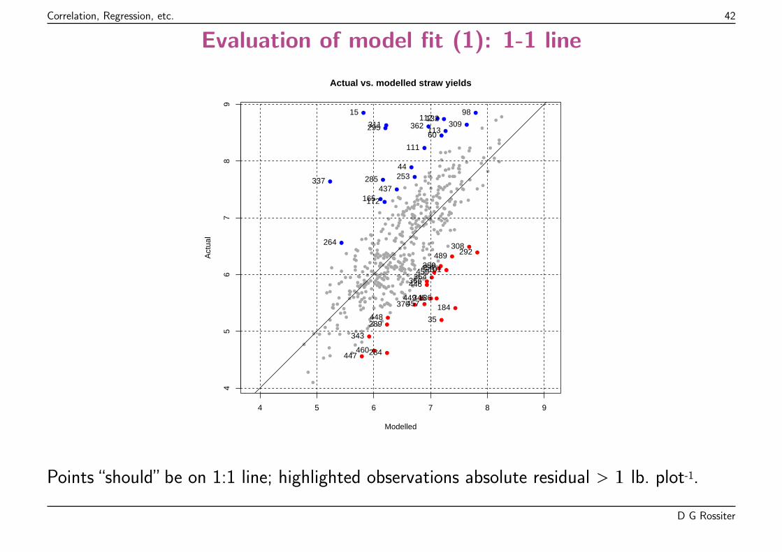
Evaluation of model fit (1): 1-1 line
●
●
●
●
●
●
●
●
●
●●
●●
●
●
●
●
●
●
●
●
●
●
●
●
●
●
●
●
●●
●
●
●
●
●
●
●
●
●
●
●●
●
●
● ●●
●
●
●
●
●
●
●
●
●
●
●
●
●
●
●
●
●
●
●
●
●●
●
●
●
●
●
●
●
●
●●
●
●
●
●
●
●
●
●
●
●
●
●
● ●
●
●
●
●
●
●
●
●
●
●
●
●
●●
●●
●
●
●
●
●
●
●
●
●
●
●
●
●
●
●
●
●
●
●
●
●
●
●
●
●
●
●
●
●
●
●
●
●
●●
●
●
●
●
●
●●
●
●
●
●
●
●
●
●
●
●
●
●
●
●
●
●
●●
●
●●
●
●
●
●
●
●
●
●
●
●
●
●
●
●●
●
●● ●●
●
●
●
●
●
●
●
●
●
●
●
●
●
●
●
●
●
●
●
●
●
●
●
●
●
●
●
●
●●
●
●
●
●
●
●
●
●
●
●
●
●
●
●
●
●
●
●
●
●
●●
●
●
●
●
●
●
●
●
●
●
●
●
●
●
●
●
●
●
●
●
●●
●
●
●
●
●
● ●
●
●
●
●
●
●
●
●
●
●
●
●
●
●
●
●
●●
●
●
●
●
●
●
●
● ●
●
●
●
●
●
●
●
●
●
●
●
●
●
●
●
●
●
●
●
●
●
●
●
●
●
●
●
●
●
●
●
●
●
●
●
●
●
●
●
●
●
●
●
●
●
●
●
●
●●
●
●
●
●
●
●
●
●
●
●
●
●
●
●
●
●
●
●
●
●
●
●
●
●●
● ●
●
●
●
●
●
●
●
●
●
●
●●
●
●
●
●
●●
●
●
●
●
●
●
●●
●●
●
●
●
●
●
●
●
● ●
●
●●
●
●
●
●
●
●
●
●
●
●
●
●
●
●
●
●
●
●
●
● ●
●
●
●
●
●
●
●
●
●
●●
●
●
●
●
●
●
●●
●
●
●
●
●
●
●
●
●
●
●
●
●
●
●
●●
●
●
●
●
●
●
●
●
● ●
●
●
●
●
●
●
●
●
●
●
●
●
●
●
●
4 5 6 7 8 9
45
67
89
Modelled
Act
ual
Actual vs. modelled straw yields
15
35
44
60
98
101
111
112
113
132
165172
184186
253
264
284
285
289
292
295
308
309311
337
343
345
362
364366
370
389
437
446
447
448
449
454
457
459
460
489
Points “should” be on 1:1 line; highlighted observations absolute residual > 1 lb. plot-1.
D G Rossiter
Correlation, Regression, etc. 43
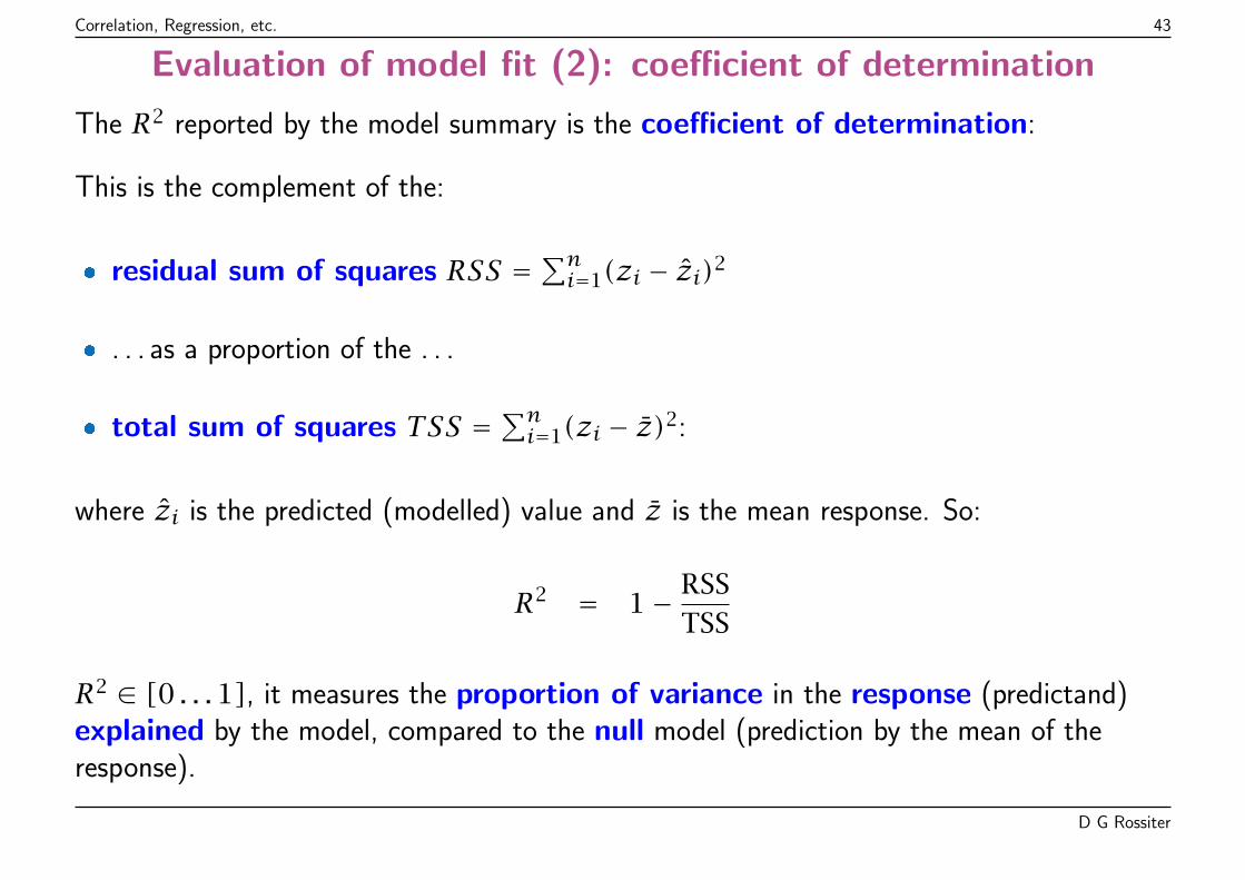
Evaluation of model fit (2): coefficient of determination
The R2 reported by the model summary is the coefficient of determination:
This is the complement of the:
� residual sum of squares RSS =∑ni=1(zi − zi)2
� . . . as a proportion of the . . .
� total sum of squares TSS =∑ni=1(zi − z)2:
where zi is the predicted (modelled) value and z is the mean response. So:
R2 = 1− RSSTSS
R2 ∈ [0 . . .1], it measures the proportion of variance in the response (predictand)explained by the model, compared to the null model (prediction by the mean of theresponse).
D G Rossiter
Correlation, Regression, etc. 44
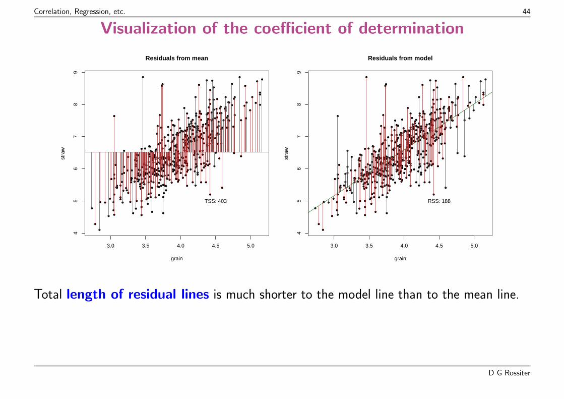
Visualization of the coefficient of determination
●
●
●
●
●
●
●
●
●
●●
●●
●
●
●
●
●
●
●
●
●
●
●
●
●
●
●
●
●●
●
●
●
●
●
●
●
●
●
●
●●
●
●
● ●●
●
●
●
●
●
●
●
●
●
●
●
●
●
●
●
●
●
●
●
●
●●
●
●
●
●
●
●
●
●
●●
●
●
●
●
●
●
●
●
●
●
●
●
● ●
●
●
●
●
●
●
●
●
●
●
●
●
●●
●●
●
●
●
●
●
●
●
●
●
●
●
●
●
●
●
●
●
●
●
●
●
●
●
●
●
●
●
●
●
●
●
●
●
●●
●
●
●
●
●
●●
●
●
●
●
●
●
●
●
●●
●
●
●
●
●
●
●●
●
●
●
●
●
●
●
●
●
●
●
●
●
●
●
●
●●
●
●● ●●
●
●
●
●
●
●
●
●
●
●
●
●
●
●
●
●
●
●
●
●
●
●
●
●
●
●
●
●
●●
●
●
●
●
●
●
●
●
●
●
●
●
●
●
●
●
●
●
●
●
●●
●
●
●
●
●
●
●
●
●
●
●
●
●
●
●
●
●
●
●
●
●●
●
●
●●
●
● ●
●
●
●
●
●
●
●
●
●
●
●
●
●
●
●
●
●●
●
●
●
●
●
●
●
● ●
●
●
●
●
●
●
●
●
●
●
●
●
●
●
●
●
●
●
●
●
●
●
●
●
●
●
●
●
●
●
●
●
●
●
●
●
●
●
●
●
●
●
●
●
●
●
●
●
●●
●
●
●
●
●
●
●
●
●
●
●
●
●
●
●
●
●
●
●
●
●
●
●
●●
● ●
●
●
●
●
●
●
●
●
●
●
●●
●
●
●
●
●●
●
●
●
●
●
●
●●
●●
●
●
●
●
●
●
●
● ●
●
●●
●
●
●
●
●
●
●
●
●
●
●
●
●●
●
●
●
●
●
● ●
●
●
●
●
●
●
●
●
●
●●
●
●
●
●
●
●
●●
●
●
●
●
●
●
●
●
●
●
●
●
●
●
●
●●
●
●
●
●
●
●
●
●
● ●
●
●
●
●
●
●
●
●
●
●
●
●
●
●
●
3.0 3.5 4.0 4.5 5.0
45
67
89
grain
stra
wResiduals from mean
TSS: 403
●
●
●
●
●
●
●
●
●
●●
●●
●
●
●
●
●
●
●
●
●
●
●
●
●
●
●
●
●●
●
●
●
●
●
●
●
●
●
●
●●
●
●
● ●●
●
●
●
●
●
●
●
●
●
●
●
●
●
●
●
●
●
●
●
●
●●
●
●
●
●
●
●
●
●
●●
●
●
●
●
●
●
●
●
●
●
●
●
● ●
●
●
●
●
●
●
●
●
●
●
●
●
●●
●●
●
●
●
●
●
●
●
●
●
●
●
●
●
●
●
●
●
●
●
●
●
●
●
●
●
●
●
●
●
●
●
●
●
●●
●
●
●
●
●
●●
●
●
●
●
●
●
●
●
●●
●
●
●
●
●
●
●●
●
●
●
●
●
●
●
●
●
●
●
●
●
●
●
●
●●
●
●● ●●
●
●
●
●
●
●
●
●
●
●
●
●
●
●
●
●
●
●
●
●
●
●
●
●
●
●
●
●
●●
●
●
●
●
●
●
●
●
●
●
●
●
●
●
●
●
●
●
●
●
●●
●
●
●
●
●
●
●
●
●
●
●
●
●
●
●
●
●
●
●
●
●●
●
●
●●
●
● ●
●
●
●
●
●
●
●
●
●
●
●
●
●
●
●
●
●●
●
●
●
●
●
●
●
● ●
●
●
●
●
●
●
●
●
●
●
●
●
●
●
●
●
●
●
●
●
●
●
●
●
●
●
●
●
●
●
●
●
●
●
●
●
●
●
●
●
●
●
●
●
●
●
●
●
●●
●
●
●
●
●
●
●
●
●
●
●
●
●
●
●
●
●
●
●
●
●
●
●
●●
● ●
●
●
●
●
●
●
●
●
●
●
●●
●
●
●
●
●●
●
●
●
●
●
●
●●
●●
●
●
●
●
●
●
●
● ●
●
●●
●
●
●
●
●
●
●
●
●
●
●
●
●●
●
●
●
●
●
● ●
●
●
●
●
●
●
●
●
●
●●
●
●
●
●
●
●
●●
●
●
●
●
●
●
●
●
●
●
●
●
●
●
●
●●
●
●
●
●
●
●
●
●
● ●
●
●
●
●
●
●
●
●
●
●
●
●
●
●
●
3.0 3.5 4.0 4.5 5.0
45
67
89
grain
stra
w
Residuals from model
RSS: 188
Total length of residual lines is much shorter to the model line than to the mean line.
D G Rossiter
Correlation, Regression, etc. 45
Calibration vs. validation
Goodness-of-fit only measures the success of calibration to the particular sampledataset.
We are actually interested in validation of the model over the whole population
� sample vs. population: representativeness, sample size
D G Rossiter
Correlation, Regression, etc. 46
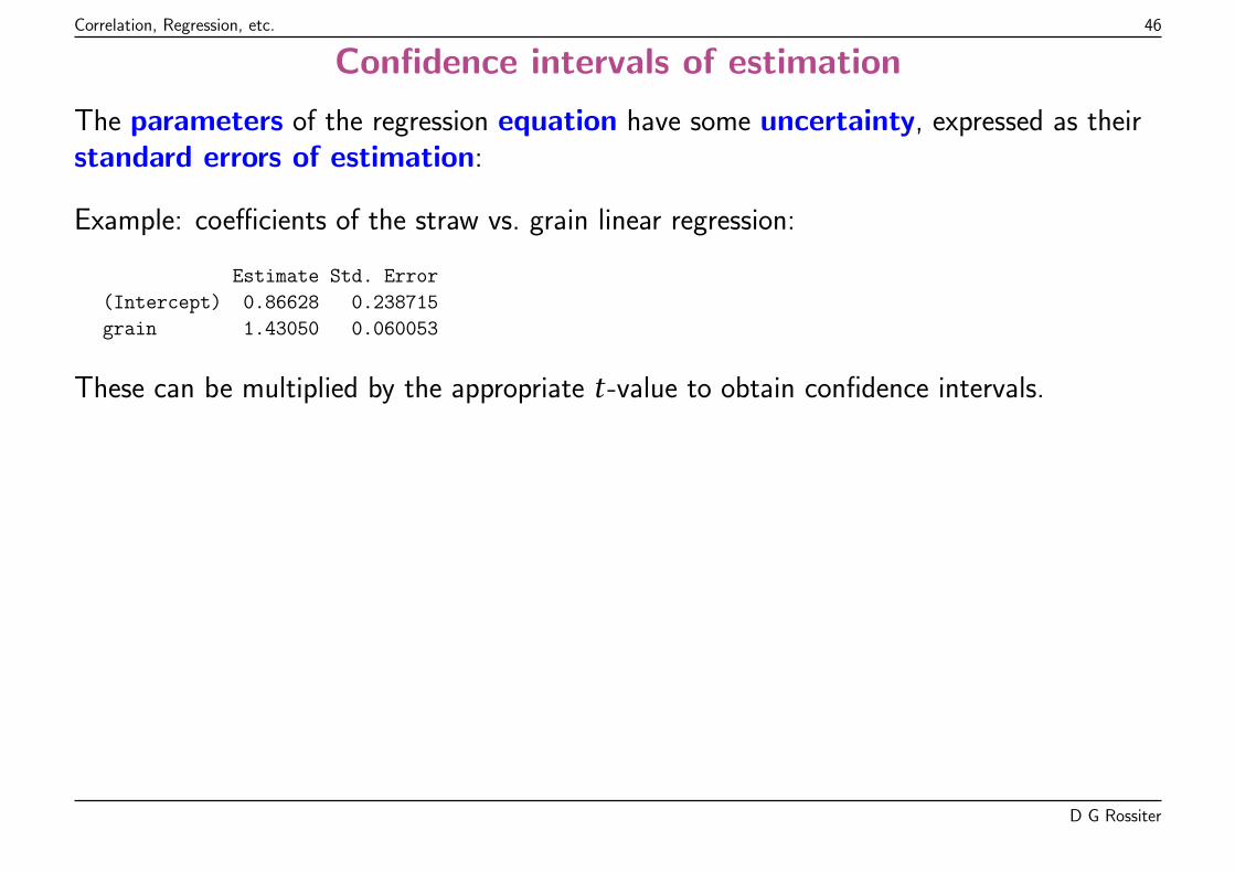
Confidence intervals of estimation
The parameters of the regression equation have some uncertainty, expressed as theirstandard errors of estimation:
Example: coefficients of the straw vs. grain linear regression:
Estimate Std. Error
(Intercept) 0.86628 0.238715
grain 1.43050 0.060053
These can be multiplied by the appropriate t-value to obtain confidence intervals.
D G Rossiter
Correlation, Regression, etc. 47
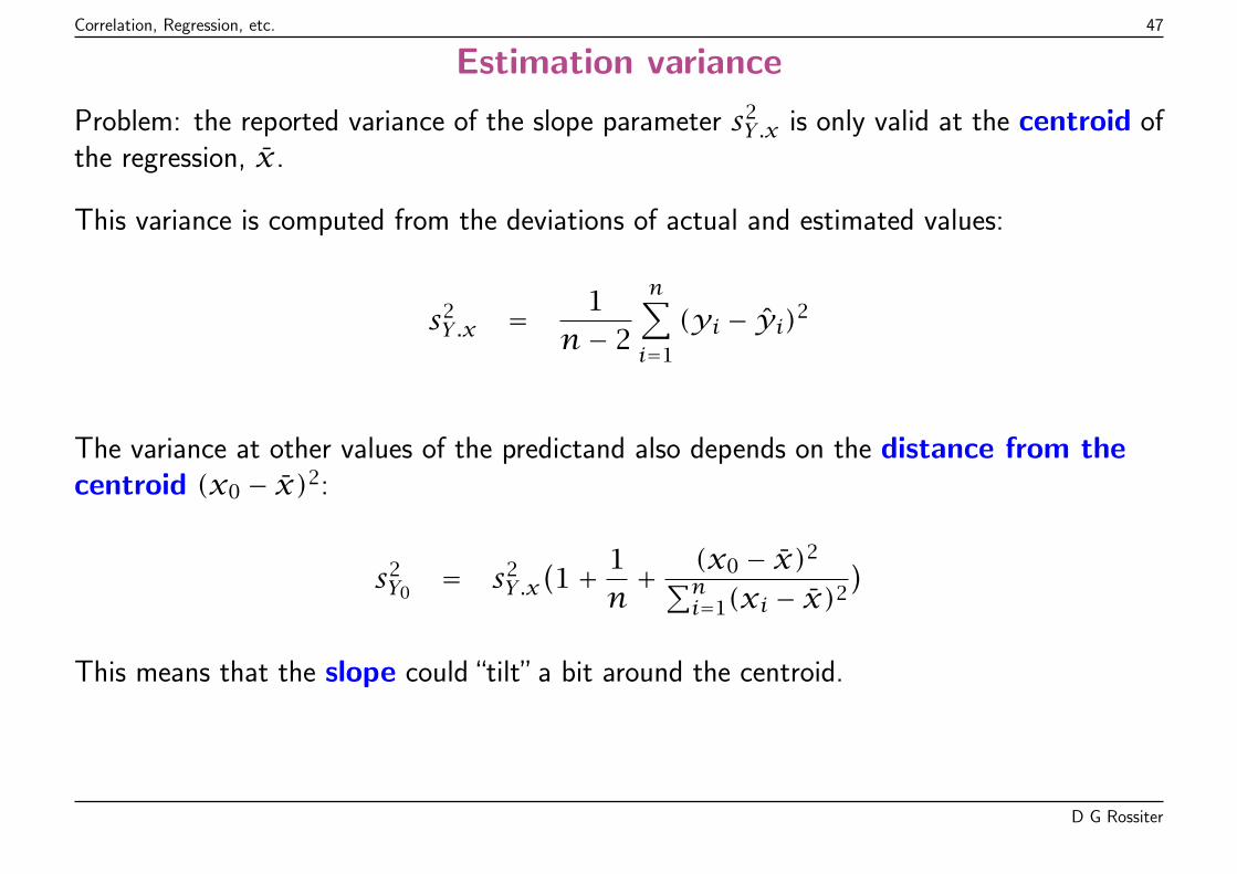
Estimation variance
Problem: the reported variance of the slope parameter s2Y .x is only valid at the centroid of
the regression, x.
This variance is computed from the deviations of actual and estimated values:
s2Y .x = 1
n− 2
n∑i=1
(yi − yi)2
The variance at other values of the predictand also depends on the distance from thecentroid (x0 − x)2:
s2Y0
= s2Y .x(1+ 1
n+ (x0 − x)2∑n
i=1(xi − x)2)
This means that the slope could “tilt” a bit around the centroid.
D G Rossiter
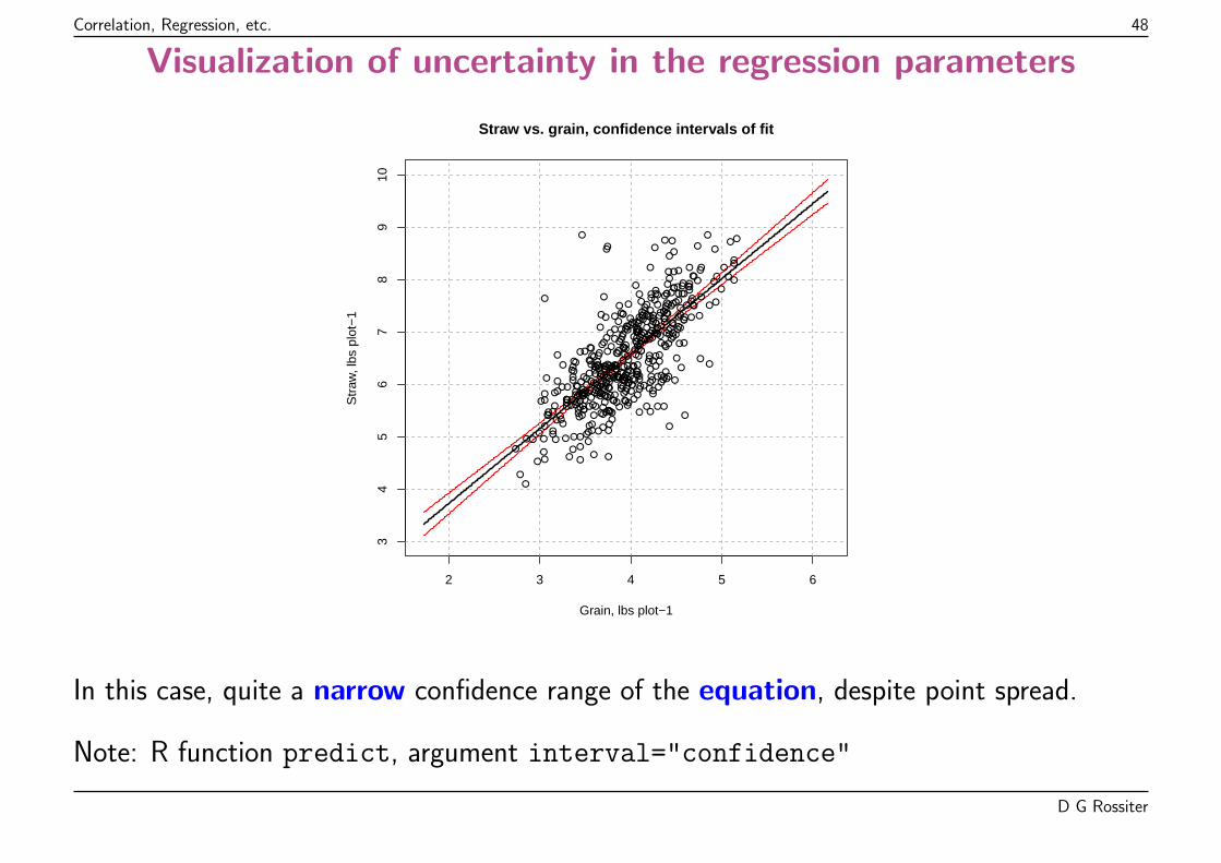
Correlation, Regression, etc. 48
Visualization of uncertainty in the regression parameters
2 3 4 5 6
34
56
78
910
Grain, lbs plot−1
Str
aw, l
bs p
lot−
1
Straw vs. grain, confidence intervals of fit
●●
●●
●
●
●
●
●
●●
● ●●
●
●
●●
●
●
●
●
●
●
●
●
●●
●
●●●
●
●
●
●
●
●
●
●
●
● ●
●
●
● ●●
●
●
●
●●
●
●
●●
●
●
●
●
●
●
●
●●
●
●
●●
●
●
●
●
●
●
●
●
●●
●
●●
●
●●
●
●●
●●
●
● ●
●●
●
●
●
●
●
●
●
●
●
●● ●
● ●
●
●
●
●
●
●●
●
●
●
●
●
●
●
●
●
●
●
●
●
●
●
●
●
●
●
●●
●
●
●
●
●
●●
●
●
●
●
●
● ●
●●
●
●
●
●●
●
●●
●●
●
●
●
●
●●
●
●●
●●
●●
●
●●
●
●
●
●
●
●
●●
●
●● ● ●
●
●
●
●
●
●
●●
●●
●
●
●
●●
●
●
●
●
●
●
●
●
●
●
●
●
●
●●
●
●
●
●
●
●
●
●
●
●
●
●
●
●
●
●●
●
●
●●●
●
●
●
●
●
●●
●
●●
●
●
●
●●
●
●
●
●
●
●●
●
●
●●
●
● ●
●
●
●●
●
●
●
●
●
●
●
●
●●
●
●
● ●
●
●
●
●
●
●
●
● ●●
●
●
●●
●
●
●
●
●
●
●
●
●
●
●
●
●●
●●
●
●
●
●
●
●●
●
●
●
●
●
●
●
●
●
●
●
●
●
●
●
●
●●
●
●●●
●
●●
●
●
●
●
●
●
●
●
●
●
●
●
●
●
●
●
●
●
●●
● ●
● ●
●
●
●
●
●
●
●●
●
●
●●
●
●
●
●
● ●●
●●
●
●
●
●●
● ●
●
●●
●
●
●
●
● ●
●
●●
●
●
●●
●
●
●
●
●
●●
●
●●
●●
●
●
●
● ●●
●
●
●
●
●
●
●
●
●●
●●
●
●
●
●
●●
●
●
●●
●
●
●●
●
●
●
●
●
●
●●●
●
●
●
●
●
●
●
●
● ●
●
●
●
●
●
●
●
●
●
●
●
●
●
●
●
In this case, quite a narrow confidence range of the equation, despite point spread.
Note: R function predict, argument interval="confidence"
D G Rossiter
Correlation, Regression, etc. 49
Prediction
One use of the fitted regression equation is to predict at arbitrary values of the predictor.
This could apply to future events or observed values of the predictor, where theestimated value of the predictand is wanted.
Example: Grain has been measured but not straw, what is the likely straw yield for a grainyield of 3 lbs plot-1?
Best-fit line: straw = 0.87 + 1.43 * grain
Direct calculation:
> 0.87 + 1.43 * 3
[1] 5.16
[1] "Predicted straw yield for grain yield 3 lbs plot-1: 5.16 lbs plot-1"
D G Rossiter
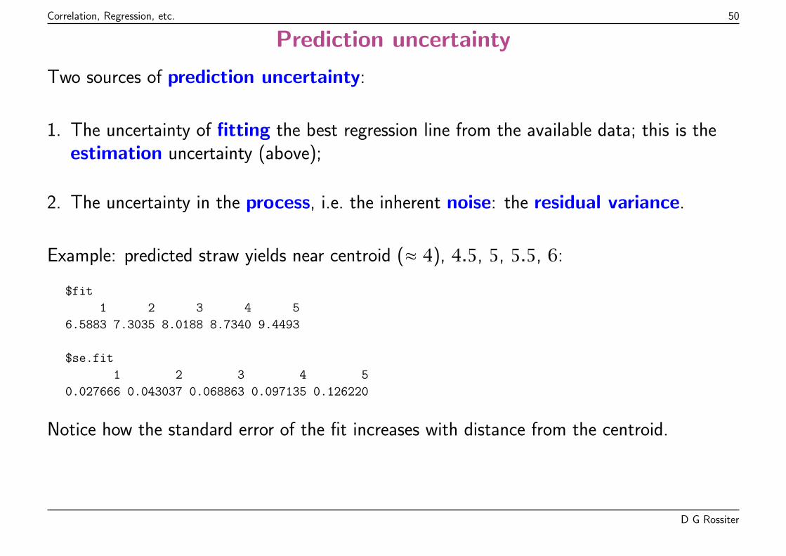
Correlation, Regression, etc. 50
Prediction uncertainty
Two sources of prediction uncertainty:
1. The uncertainty of fitting the best regression line from the available data; this is theestimation uncertainty (above);
2. The uncertainty in the process, i.e. the inherent noise: the residual variance.
Example: predicted straw yields near centroid (≈ 4), 4.5, 5, 5.5, 6:
$fit
1 2 3 4 5
6.5883 7.3035 8.0188 8.7340 9.4493
$se.fit
1 2 3 4 5
0.027666 0.043037 0.068863 0.097135 0.126220
Notice how the standard error of the fit increases with distance from the centroid.
D G Rossiter
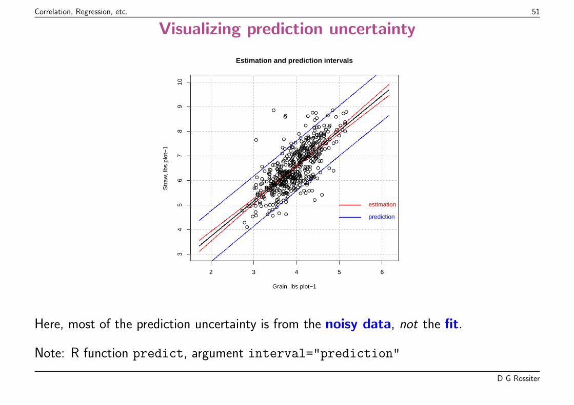
Correlation, Regression, etc. 51
Visualizing prediction uncertainty
2 3 4 5 6
34
56
78
910
Grain, lbs plot−1
Str
aw, l
bs p
lot−
1
Estimation and prediction intervals
●●
●●
●
●
●
●
●
●●
● ●●
●
●
●●
●
●
●
●
●
●
●
●
●●
●
●●●
●
●
●
●
●
●
●
●
●
● ●
●
●
● ●●
●
●
●
●●
●
●
●●
●
●
●
●
●
●
●
●●
●
●
●●
●
●
●
●
●
●
●
●
●●
●
●●
●
●●
●
●●
●●
●
● ●
●●
●
●
●
●
●
●
●
●
●
●● ●
● ●
●
●
●
●
●
●●
●
●
●
●
●
●
●
●
●
●
●
●
●
●
●
●
●
●
●
●●
●
●
●
●
●
●●
●
●
●
●
●
● ●
●●
●
●
●
●●
●
●●
●●
●
●
●
●
●●
●
●●
●●
●●
●
●●
●
●
●
●
●
●
●●
●
●● ● ●
●
●
●
●
●
●
●●
●●
●
●
●
●●
●
●
●
●
●
●
●
●
●
●
●
●
●
●●
●
●
●
●
●
●
●
●
●
●
●
●
●
●
●
●●
●
●
●●●
●
●
●
●
●
●●
●
●●
●
●
●
●●
●
●
●
●
●
●●
●
●
●●
●
● ●
●
●
●●
●
●
●
●
●
●
●
●
●●
●
●
● ●
●
●
●
●
●
●
●
● ●●
●
●
●●
●
●
●
●
●
●
●
●
●
●
●
●
●●
●●
●
●
●
●
●
●●
●
●
●
●
●
●
●
●
●
●
●
●
●
●
●
●
●●
●
●●●
●
●●
●
●
●
●
●
●
●
●
●
●
●
●
●
●
●
●
●
●
●●
● ●
● ●
●
●
●
●
●
●
●●
●
●
●●
●
●
●
●
● ●●
●●
●
●
●
●●
● ●
●
●●
●
●
●
●
● ●
●
●●
●
●
●●
●
●
●
●
●
●●
●
●●
●●
●
●
●
● ●●
●
●
●
●
●
●
●
●
●●
●●
●
●
●
●
●●
●
●
●●
●
●
●●
●
●
●
●
●
●
●●●
●
●
●
●
●
●
●
●
● ●
●
●
●
●
●
●
●
●
●
●
●
●
●
●
●
estimation
prediction
Here, most of the prediction uncertainty is from the noisy data, not the fit.
Note: R function predict, argument interval="prediction"
D G Rossiter

Correlation, Regression, etc. 52
Topic: Model evaluation
(Often called “validation”)
Measures of model quality:
� internal : the data used to build the model is also used to evaluate it
* goodness-of-fit; adjusted for dataset size and number of parameters, e.g., AIC,adjusted R2
* not a true test of predictive accuracy
� external: evaluate with independent data from the same population
* a completely different set* part of a single set: split the dataset into a “calibration” and a “validation” set
� cross-validation (“jackknifing”)
* one dataset, repeated split, recalibration, compare predicted with actual
D G Rossiter
Correlation, Regression, etc. 53
1:1 Evaluation
1. The model is developed using only the observations in the calibration set;
2. This model is used to predict at the the observations in the validation set, using theactual (measured) values of the predictor (independent) variable(s);
3. These predicted values are compared to the actual (measured) values of the response(dependent) variable in the validation set.
This relation should be exactly 1:1
D G Rossiter
Correlation, Regression, etc. 54
Splitting a dataset
Tradeoff:
1. The calibration set must be large enough reliable modelling;
2. The validation set must be large enough for reliable validation statistics.
A common split in a medium-size dataset (100–500 observations) is 3 to 1, i.e., 3/4 forcalibration and 1/4 for validation.
Select observations for each set:
� random: select at random (without replacement); this requires no assumptions aboutthe sequence of items in the dataset;
� systematic: select in sequence; this requires absence of serial correlation, i.e., thatobservations listed in sequence be independent;
� stratified: first divide the observations by some factor and then apply either a randomor systematic sampling within each stratum, generally proportional to stratum size.
D G Rossiter
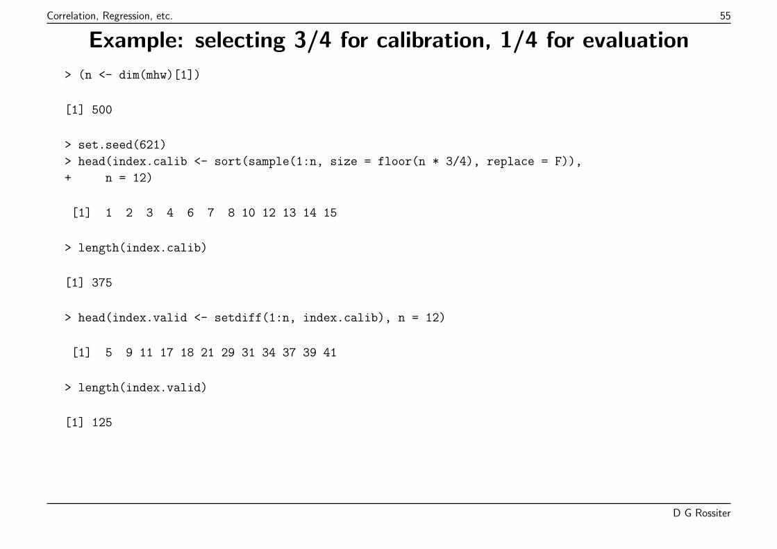
Correlation, Regression, etc. 55
Example: selecting 3/4 for calibration, 1/4 for evaluation
> (n <- dim(mhw)[1])
[1] 500
> set.seed(621)
> head(index.calib <- sort(sample(1:n, size = floor(n * 3/4), replace = F)),
+ n = 12)
[1] 1 2 3 4 6 7 8 10 12 13 14 15
> length(index.calib)
[1] 375
> head(index.valid <- setdiff(1:n, index.calib), n = 12)
[1] 5 9 11 17 18 21 29 31 34 37 39 41
> length(index.valid)
[1] 125
D G Rossiter
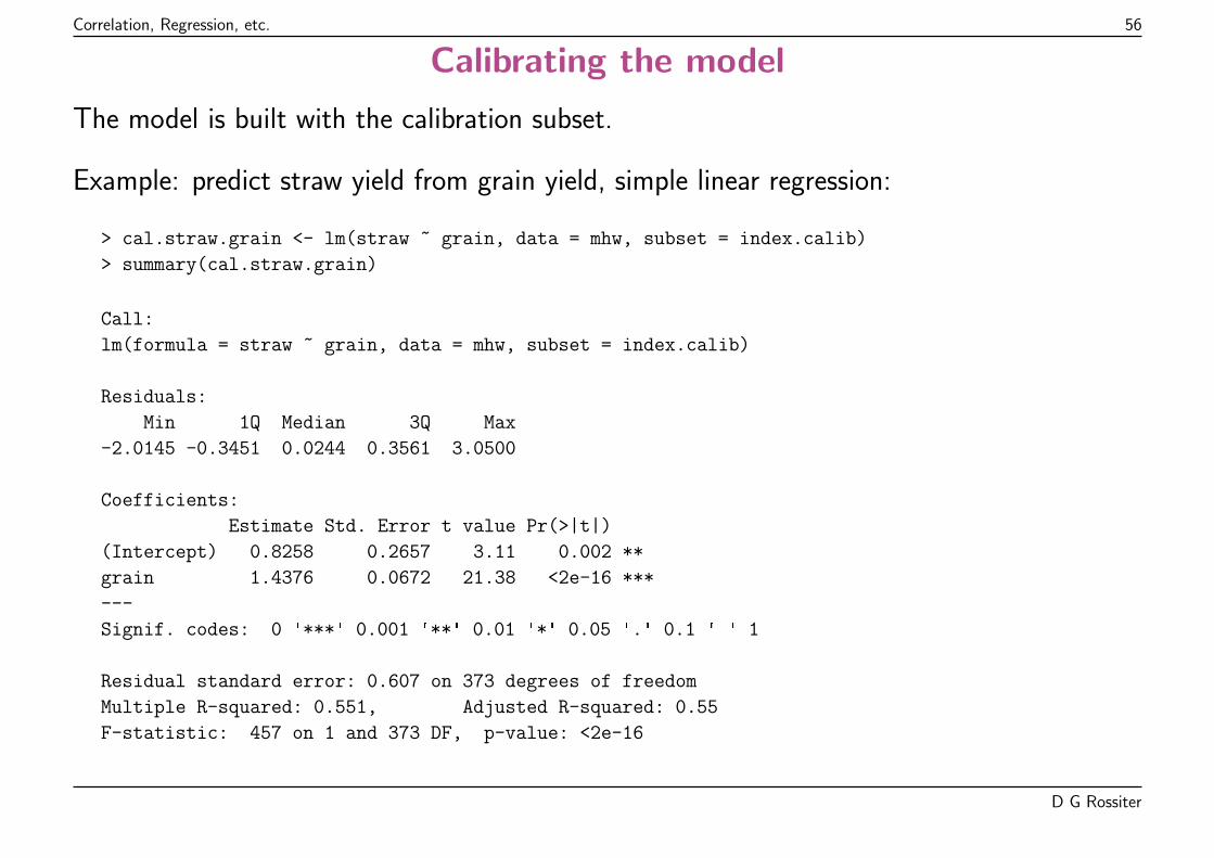
Correlation, Regression, etc. 56
Calibrating the model
The model is built with the calibration subset.
Example: predict straw yield from grain yield, simple linear regression:
> cal.straw.grain <- lm(straw ~ grain, data = mhw, subset = index.calib)
> summary(cal.straw.grain)
Call:
lm(formula = straw ~ grain, data = mhw, subset = index.calib)
Residuals:
Min 1Q Median 3Q Max
-2.0145 -0.3451 0.0244 0.3561 3.0500
Coefficients:
Estimate Std. Error t value Pr(>|t|)
(Intercept) 0.8258 0.2657 3.11 0.002 **
grain 1.4376 0.0672 21.38 <2e-16 ***
---
Signif. codes: 0 '***' 0.001 '**' 0.01 '*' 0.05 '.' 0.1 ' ' 1
Residual standard error: 0.607 on 373 degrees of freedom
Multiple R-squared: 0.551, Adjusted R-squared: 0.55
F-statistic: 457 on 1 and 373 DF, p-value: <2e-16
D G Rossiter
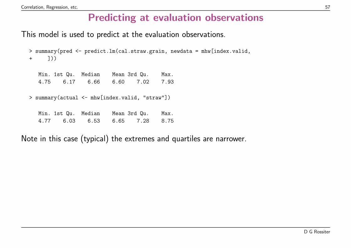
Correlation, Regression, etc. 57
Predicting at evaluation observations
This model is used to predict at the evaluation observations.
> summary(pred <- predict.lm(cal.straw.grain, newdata = mhw[index.valid,
+ ]))
Min. 1st Qu. Median Mean 3rd Qu. Max.
4.75 6.17 6.66 6.60 7.02 7.93
> summary(actual <- mhw[index.valid, "straw"])
Min. 1st Qu. Median Mean 3rd Qu. Max.
4.77 6.03 6.53 6.65 7.28 8.75
Note in this case (typical) the extremes and quartiles are narrower.
D G Rossiter
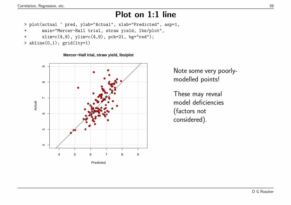
Correlation, Regression, etc. 58
Plot on 1:1 line> plot(actual ~ pred, ylab="Actual", xlab="Predicted", asp=1,
+ main="Mercer-Hall trial, straw yield, lbs/plot",
+ xlim=c(4,9), ylim=c(4,9), pch=21, bg="red");
> abline(0,1); grid(lty=1)
●●
●
●
●●
●
●
●
●
●●●
●
●●
●
●
●
●
●
●
●
●
●
●
●
● ●
●
●●
●
●
●
●●
●
●
●●
●●
●
●
●
●
●
●
●
●●●
●
●
●●
●
●●●
●
●
●●
●
●
●●
●
●
●
●
●
●
●
● ●
●
●
●
●
●
●
●
●
●
●
●●●
●
●
●
●
●
●
●
●
●
●●
●
●
● ●
●
●
● ●●
●
●
●
●
●
●
●●
●
●
●
●
●
●
4 5 6 7 8 9
45
67
89
Mercer−Hall trial, straw yield, lbs/plot
Predicted
Act
ual
Note some very poorly-modelled points!
These may revealmodel deficiencies(factors notconsidered).
D G Rossiter
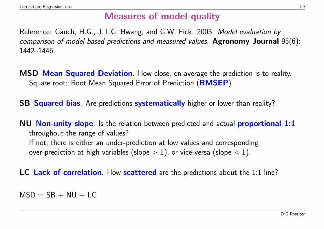
Correlation, Regression, etc. 59
Measures of model quality
Reference: Gauch, H.G., J.T.G. Hwang, and G.W. Fick. 2003. Model evaluation bycomparison of model-based predictions and measured values. Agronomy Journal 95(6):1442–1446.
MSD Mean Squared Deviation. How close, on average the prediction is to reality.Square root: Root Mean Squared Error of Prediction (RMSEP)
SB Squared bias. Are predictions systematically higher or lower than reality?
NU Non-unity slope. Is the relation between predicted and actual proportional 1:1throughout the range of values?If not, there is either an under-prediction at low values and correspondingover-prediction at high variables (slope > 1), or vice-versa (slope < 1).
LC Lack of correlation. How scattered are the predictions about the 1:1 line?
MSD = SB + NU + LC
D G Rossiter
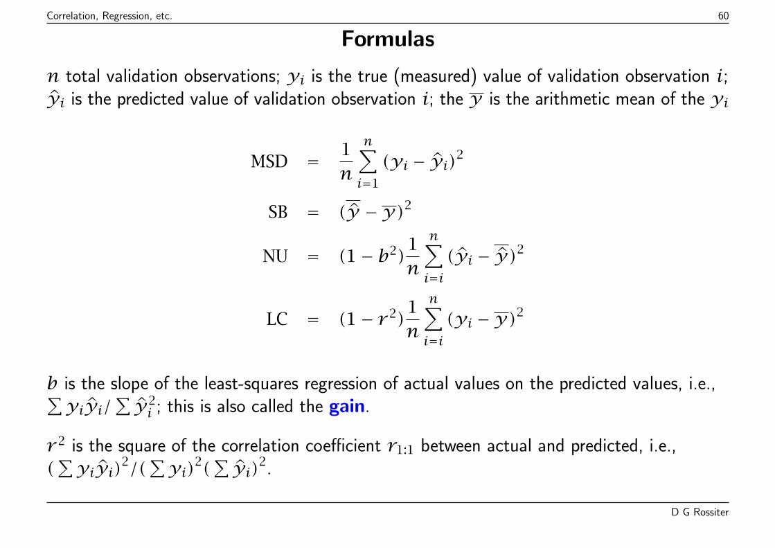
Correlation, Regression, etc. 60
Formulas
n total validation observations; yi is the true (measured) value of validation observation i;yi is the predicted value of validation observation i; the y is the arithmetic mean of the yi
MSD = 1n
n∑i=1
(yi − yi)2
SB = (y −y)2
NU = (1− b2)1n
n∑i=i(yi − y)2
LC = (1− r 2)1n
n∑i=i(yi −y)2
b is the slope of the least-squares regression of actual values on the predicted values, i.e.,∑yiyi/
∑y2i ; this is also called the gain.
r 2 is the square of the correlation coefficient r1:1 between actual and predicted, i.e.,(∑yiyi)2/(
∑yi)2(
∑yi)2.
D G Rossiter
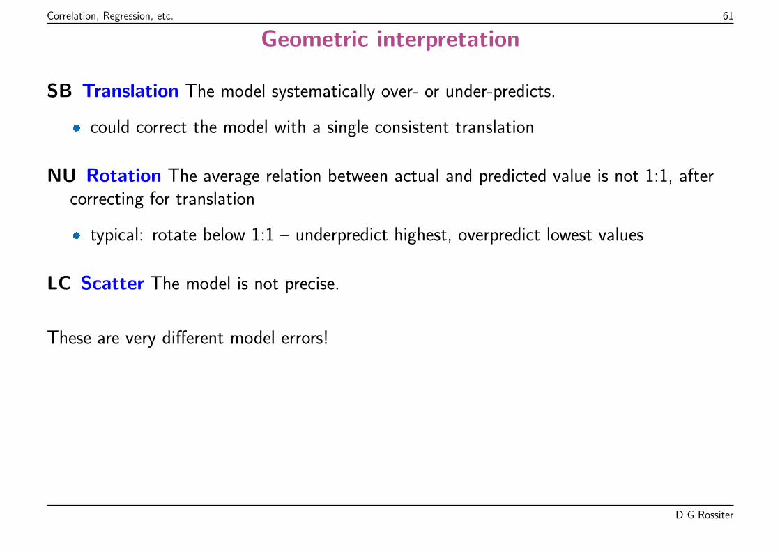
Correlation, Regression, etc. 61
Geometric interpretation
SB Translation The model systematically over- or under-predicts.
� could correct the model with a single consistent translation
NU Rotation The average relation between actual and predicted value is not 1:1, aftercorrecting for translation
� typical: rotate below 1:1 – underpredict highest, overpredict lowest values
LC Scatter The model is not precise.
These are very different model errors!
D G Rossiter
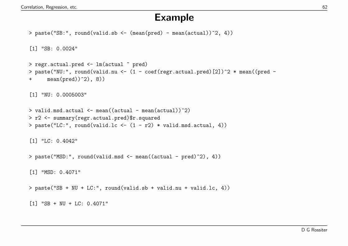
Correlation, Regression, etc. 62
Example
> paste("SB:", round(valid.sb <- (mean(pred) - mean(actual))^2, 4))
[1] "SB: 0.0024"
> regr.actual.pred <- lm(actual ~ pred)
> paste("NU:", round(valid.nu <- (1 - coef(regr.actual.pred)[2])^2 * mean((pred -
+ mean(pred))^2), 8))
[1] "NU: 0.0005003"
> valid.msd.actual <- mean((actual - mean(actual))^2)
> r2 <- summary(regr.actual.pred)$r.squared
> paste("LC:", round(valid.lc <- (1 - r2) * valid.msd.actual, 4))
[1] "LC: 0.4042"
> paste("MSD:", round(valid.msd <- mean((actual - pred)^2), 4))
[1] "MSD: 0.4071"
> paste("SB + NU + LC:", round(valid.sb + valid.nu + valid.lc, 4))
[1] "SB + NU + LC: 0.4071"
D G Rossiter
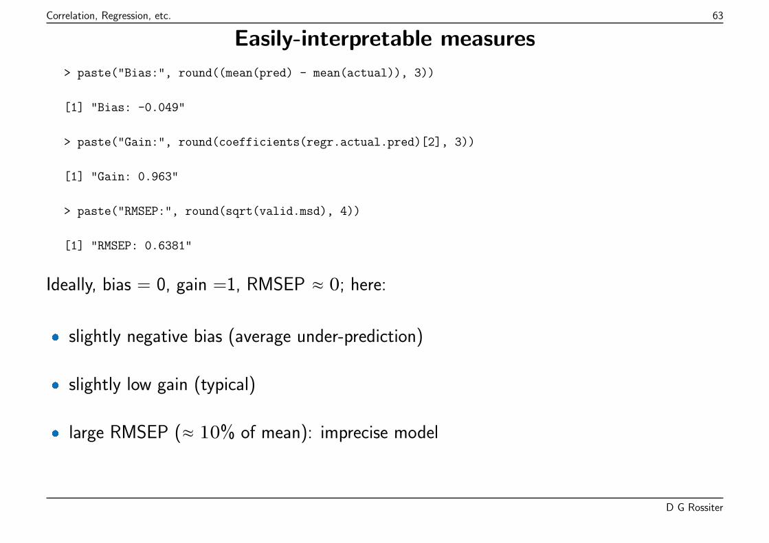
Correlation, Regression, etc. 63
Easily-interpretable measures
> paste("Bias:", round((mean(pred) - mean(actual)), 3))
[1] "Bias: -0.049"
> paste("Gain:", round(coefficients(regr.actual.pred)[2], 3))
[1] "Gain: 0.963"
> paste("RMSEP:", round(sqrt(valid.msd), 4))
[1] "RMSEP: 0.6381"
Ideally, bias = 0, gain =1, RMSEP ≈ 0; here:
� slightly negative bias (average under-prediction)
� slightly low gain (typical)
� large RMSEP (≈ 10% of mean): imprecise model
D G Rossiter
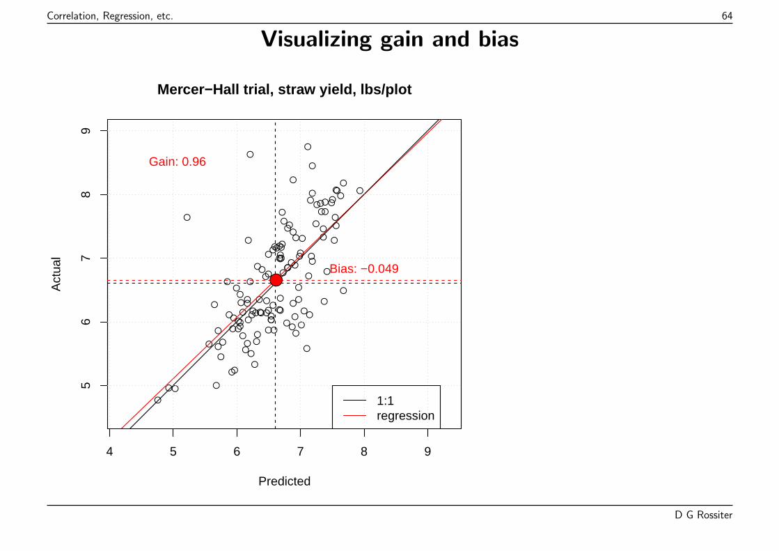
Correlation, Regression, etc. 64
Visualizing gain and bias
●●
●
●
●●
●
●
●
●
●
●●
●
●
●
●
●
●
●
●
●
●
●
●
●
●
● ●
●
●●
●
●
●
●●
●
●
●
●●
●
●
●
●
●
●
●
●
●●
●
●
●
●●
●
●●●
●
●
●●
●
●
●
●
●
●
●
●
●
●
●
●●
●
●
●
●
●
●
●
●
●
●
●●●
●
●
●
●
●
●
●
●
●
●●
●
●
● ●
●
●
● ●●
●
●
●
●
●
●
●●
●
●
●
●
●
●
4 5 6 7 8 9
56
78
9Mercer−Hall trial, straw yield, lbs/plot
Predicted
Act
ual
Gain: 0.96
●Bias: −0.049
1:1regression
D G Rossiter

Correlation, Regression, etc. 65
Topic: No-intercept models
It is possible to fit the model without an intercept, i.e., the linear relation is forced throughthe origin (0,0). The equation becomes:
yi = βxi + εi
There is only a slope to be estimated; the intercept is fixed at 0.
This is also called regression through the origin.
D G Rossiter
Correlation, Regression, etc. 66
Implications of a no-intercept model
� The mean residual is (in general) not zero;
� The residual sum-of-squares is (in general) larger than for a model with intercept;
� The usual formula for goodness-of-fit is not appropriate (see below).
Even if we know from nature that the relation must incude (0,0), this takes away a degreeof freedom from the fit, and gives a poorer fit.
D G Rossiter
Correlation, Regression, etc. 67
Appropriateness of a no-intercept model
1. There are physical reasons why the relation must include (0,0);
� e.g., no straw → no grain is possible (but not vice-versa!)
2. If non-negative variables, a negative prediction should be avoided;
� e.g., impossible to have negative straw or grain in a plot� This can also be avoided by setting any negative predictions to zero
3. The range of the observations covers (0,0) or at least is close;
� otherwise we are assuming a linear form from the origin to the range of our data,when it may have some other form, e.g., exponential, power . . . ; there is no evidencefor choosing a linear form near the origin
4. The null hypothesis H0 : β0 = 0 in a linear regression with intercept can not bedisproven (t-test of the coefficient).
D G Rossiter
Correlation, Regression, etc. 68
Fitting a no-intercept model
The slope βY .x can not be estimated from the sample covariance sXY and variance of thepredictand s2
x, because the (co)variances are relative to means, which we can notcompute (there is no degree of freedom, because of the fixed intercept).
Instead, the slope is computed by minimizes the RSS, again by orthogonal projection:b = [x′x]−1[x′y], where the design matrix x here does not have an initial column of1’s, just a column of xi.
This reduces to: ∑xiyi∑x2i
D G Rossiter
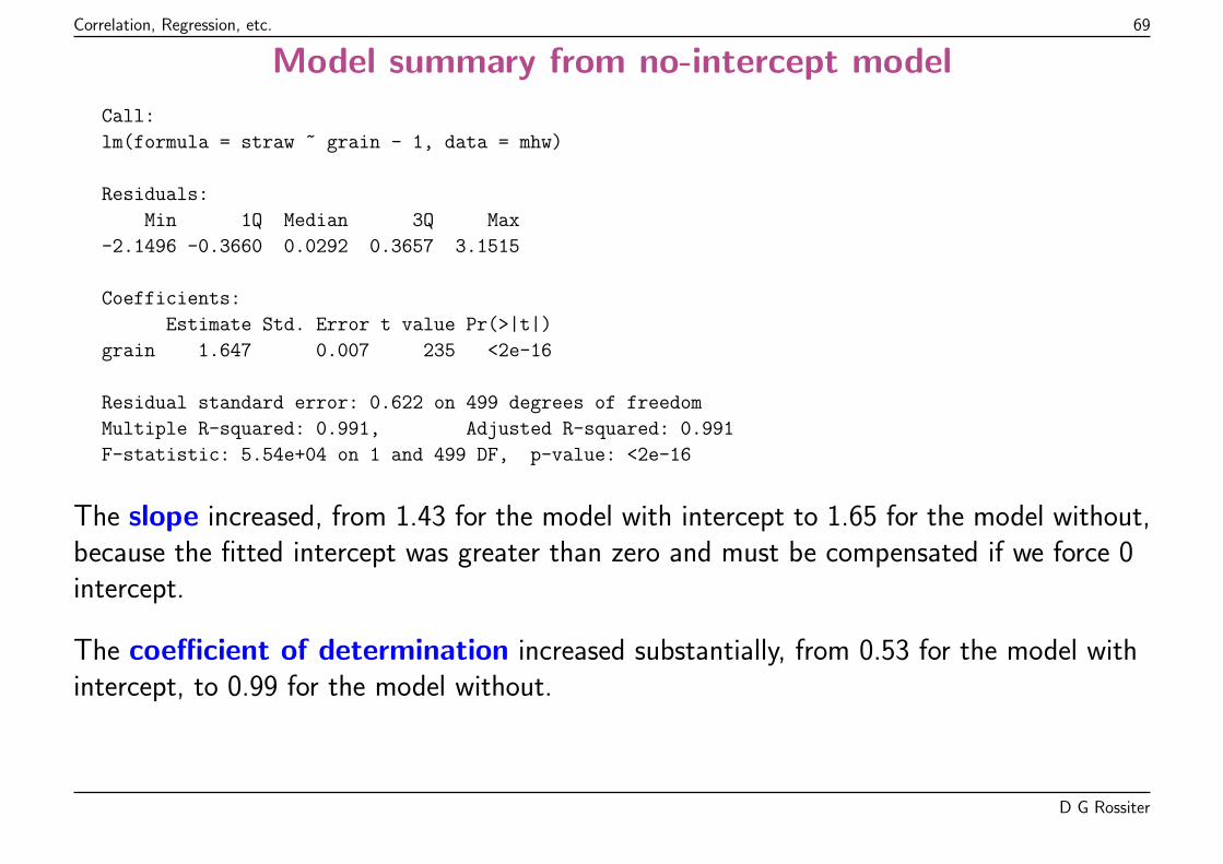
Correlation, Regression, etc. 69
Model summary from no-intercept model
Call:
lm(formula = straw ~ grain - 1, data = mhw)
Residuals:
Min 1Q Median 3Q Max
-2.1496 -0.3660 0.0292 0.3657 3.1515
Coefficients:
Estimate Std. Error t value Pr(>|t|)
grain 1.647 0.007 235 <2e-16
Residual standard error: 0.622 on 499 degrees of freedom
Multiple R-squared: 0.991, Adjusted R-squared: 0.991
F-statistic: 5.54e+04 on 1 and 499 DF, p-value: <2e-16
The slope increased, from 1.43 for the model with intercept to 1.65 for the model without,because the fitted intercept was greater than zero and must be compensated if we force 0intercept.
The coefficient of determination increased substantially, from 0.53 for the model withintercept, to 0.99 for the model without.
D G Rossiter
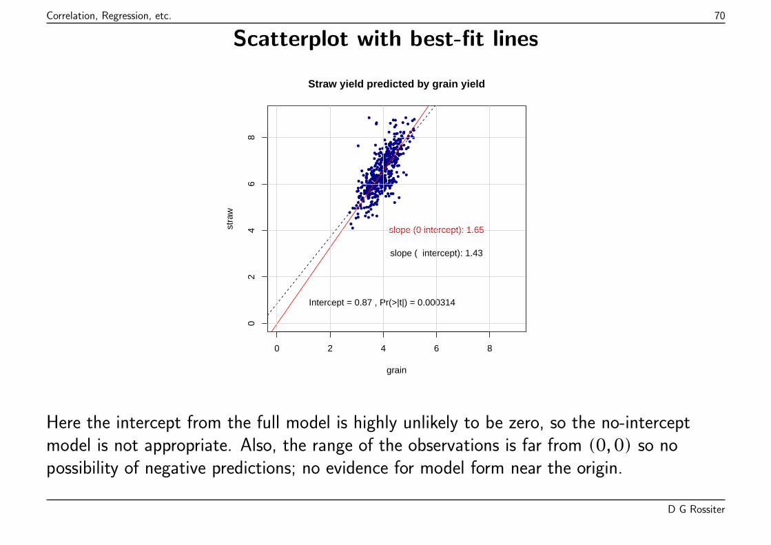
Correlation, Regression, etc. 70
Scatterplot with best-fit lines
●●
●
●
●
●
●
●
●
●●
●●●
●
●
●
●●
●
●
●
●
●
●
●
●
●
●
●●●
●
●
●
●
●
●
●
●
●
●●
●
●
● ●●
●
●
●
●
●
●
●
●
●
●
●
●
●
●
●
●
●●
●
●
●●
●
●
●
●
●
●
●
●
●●
●
●
●
●
●
●
●
●
●
●●
●
● ●
●
●
●
●
●
●
●
●
●
●
●
●● ●
●●
●
●
●
●
●
●
●●
●
●
●
●
●
●
●
●
●
●
●
●
●
●
●
●
●
●
●●
●
●
●
●
●
●●
●
●
●
●
●
●●
●●
●
●
●
●●
●
●●
●●
●
●
●
●
●●
●
●●
●
●
●
●
●
●●
●
●
●
●
●
●
●●
●
●● ●●
●
●
●
●
●
●
●
●
●●
●
●
●
●●
●
●
●
●
●
●
●
●
●
●
●
●
●
●●
●
●
●
●
●
●
●
●
●
●
●
●
●
●
●
●
●
●
●
●
●●●
●
●
●
●
●
●
●
●
●
●
●
●
●●
●
●
●
●
●
●●
●
●
●●
●
● ●
●
●
●
●
●
●
●
●
●
●
●
●
●●
●
●
● ●
●
●
●
●
●
●
●
● ●
●
●
●
●
●
●
●
●
●
●
●
●
●
●
●
●
●
●●
●●
●
●
●
●
●
●
●
●
●
●
●
●
●
●
●
●
●
●
●
●
●
●
●
●
●
●
●●●
●
●●
●
●
●
●
●
●
●
●
●
●
●
●
●
●
●
●
●
●
●
●
● ●
● ●
●
●
●
●
●
●
●
●
●
●
●●
●
●
●
●
● ●●
●●
●
●
●
●●
● ●
●
●●
●
●
●
●
● ●
●
●●
●
●
●
●
●
●
●
●
●
●
●●
●●
●
●
●
●
●
● ●●
●
●
●
●
●
●
●
●
●●
●
●
●
●
●
●
●●
●
●
●
●
●
●
●●
●
●
●
●
●
●
●●●
●
●
●
●
●
●
●
●
● ●
●
●
●
●
●
●
●
●
●
●
●
●
●
●
●
0 2 4 6 8
02
46
8
grain
stra
w
Straw yield predicted by grain yield
slope (0 intercept): 1.65
slope ( intercept): 1.43
Intercept = 0.87 , Pr(>|t|) = 0.000314
Here the intercept from the full model is highly unlikely to be zero, so the no-interceptmodel is not appropriate. Also, the range of the observations is far from (0,0) so nopossibility of negative predictions; no evidence for model form near the origin.
D G Rossiter
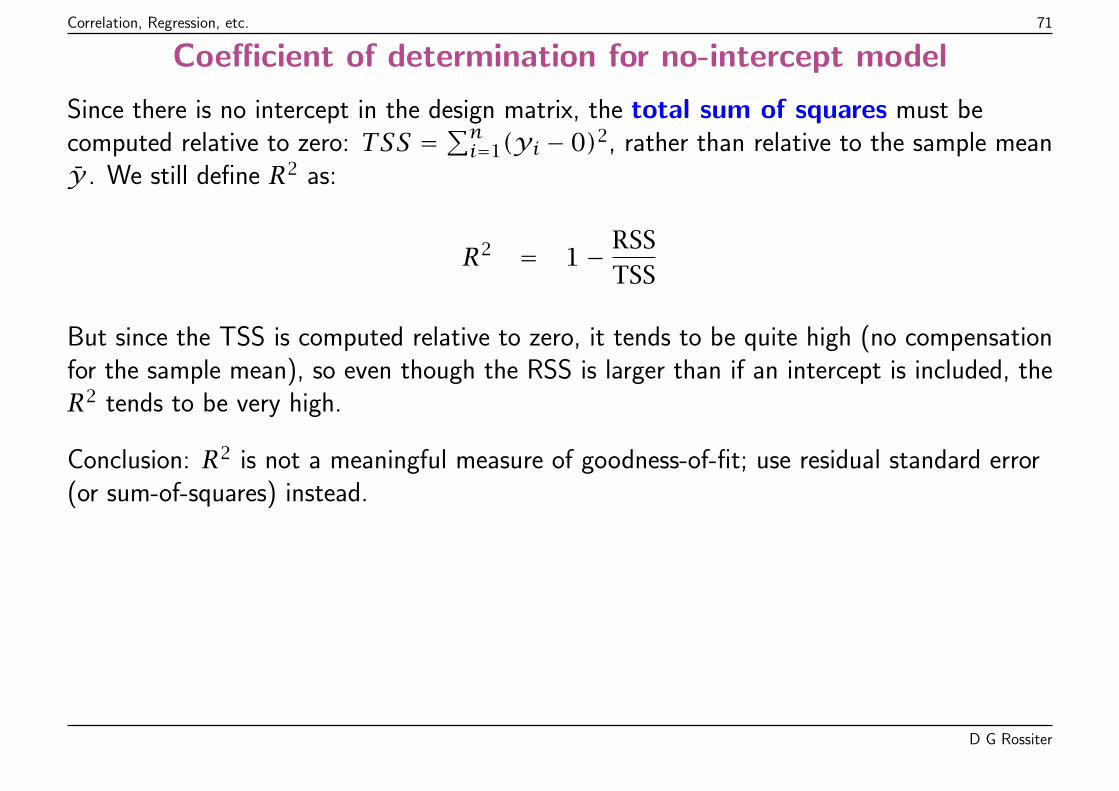
Correlation, Regression, etc. 71
Coefficient of determination for no-intercept model
Since there is no intercept in the design matrix, the total sum of squares must becomputed relative to zero: TSS =
∑ni=1(yi − 0)2, rather than relative to the sample mean
y . We still define R2 as:
R2 = 1− RSSTSS
But since the TSS is computed relative to zero, it tends to be quite high (no compensationfor the sample mean), so even though the RSS is larger than if an intercept is included, theR2 tends to be very high.
Conclusion: R2 is not a meaningful measure of goodness-of-fit; use residual standard error(or sum-of-squares) instead.
D G Rossiter
Correlation, Regression, etc. 72
Topic: Structural analysis
Recall:
1. Variables have different status
(a) A univariate linear regression of straw (dependent) on grain (independent) yield;(b) A univariate linear regression of grain (dependent) on straw (independent) yield.
2. Variables are of equal status
(a) A bivariate linear correlation between the two variables (straw and grain yields);(b) A linear structural relation between the two yields.
“Structure”: underlying relation between two variables, considered equally.
D G Rossiter
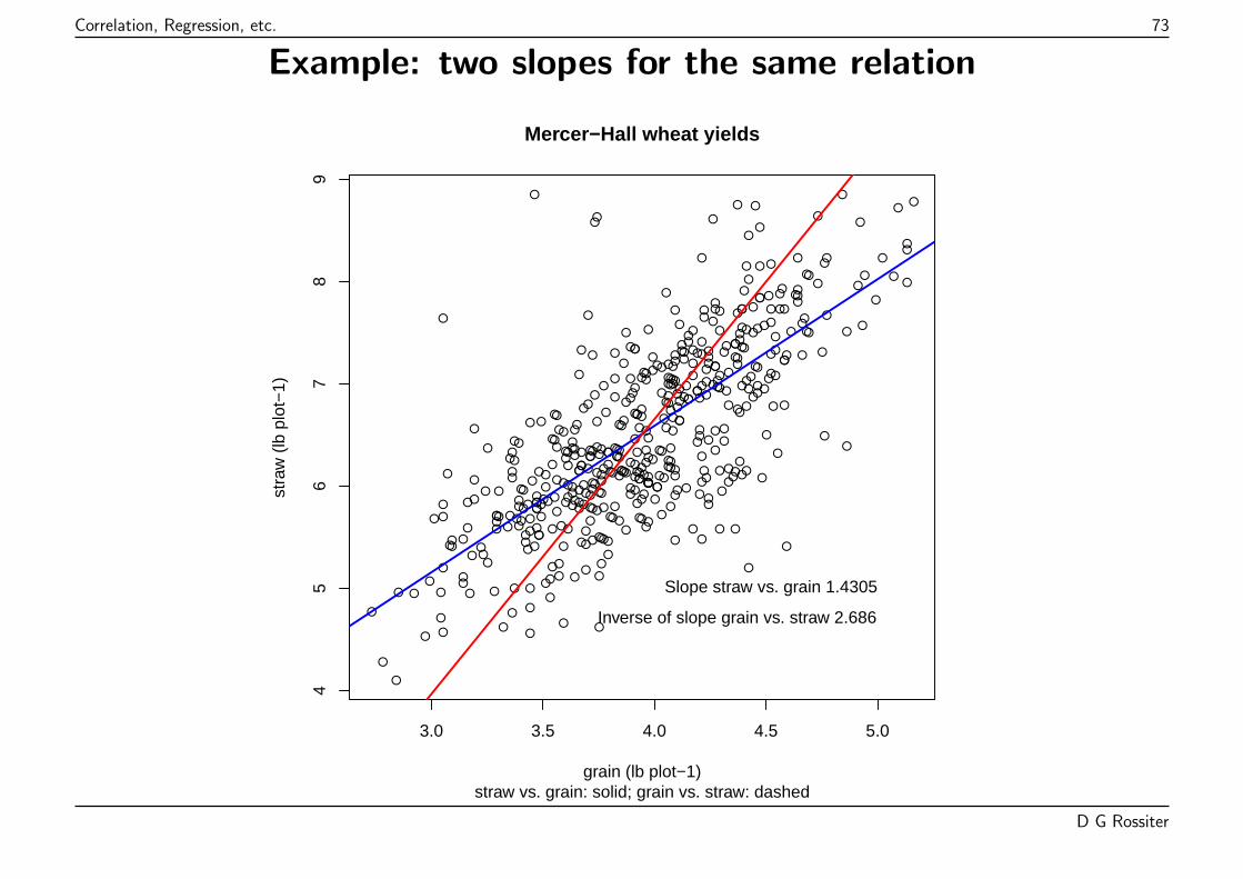
Correlation, Regression, etc. 73
Example: two slopes for the same relation
●
●
●
●
●
●
●
●
●
●●
● ●●
●
●
●
●
●
●
●
●
●
●
●
●
●
●
●
●●
●
●
●
●
●
●
●
●
●
●
●●
●
●
● ●●
●
●
●
●
●
●
●
●
●
●
●
●
●
●
●
●
●●
●
●
●●
●
●
●
●
●
●
●
●
●●
●
●
●
●
●
●
●
●
●
●
●
●
● ●
●
●
●
●
●
●
●
●
●
●
●
●● ●
● ●
●
●
●
●
●
●
●●
●
●
●
●
●
●
●
●
●
●
●
●
●
●
●
●
●
●
●●
●
●
●
●
●
●●
●
●
●
●
●
●●
●●
●
●
●
●
●
●
●●
●
●
●
●
●
●
●●
●
●●
●
●
●
●
●
●●
●
●
●
●
●
●
●●
●
●● ●●
●
●
●
●
●
●
●
●
●●
●
●
●
●●
●
●
●
●
●
●
●
●
●
●
●
●
●
●●
●
●
●
●
●
●
●
●
●
●
●
●
●
●
●
●
●
●
●
●
●●
●
●
●
●
●
●
●
●
●
●
●
●
●
●
●
●
●
●
●
●
●●
●
●
●●
●
● ●
●
●
●
●
●
●
●
●
●
●
●
●
●
●
●
●
●●
●
●
●
●
●
●
●
● ●
●
●
●
●
●
●
●
●
●
●
●
●
●
●
●
●
●
●●
●●
●
●
●
●
●
●
●
●
●
●
●
●
●
●
●
●
●
●
●
●
●
●
●
●
●
●
●●●
●
●●
●
●
●
●
●
●
●
●
●
●
●
●
●
●
●
●
●
●
●
●
●●
● ●
●
●
●
●
●
●
●
●
●
●
●●
●
●
●
●
● ●●
●
●
●
●
●
●●
● ●
●
●●
●
●
●
●
● ●
●
●●
●
●
●
●
●
●
●
●
●
●
●●
●●
●
●
●
●
●
● ●●
●
●
●
●
●
●
●
●
●●
●
●
●
●
●
●
●●
●
●
●
●
●
●
●●
●
●
●
●
●
●
●●●
●
●
●
●
●
●
●
●
● ●
●
●
●
●
●
●
●
●
●
●
●
●
●
●
●
3.0 3.5 4.0 4.5 5.0
45
67
89
Mercer−Hall wheat yields
grain (lb plot−1)
stra
w (
lb p
lot−
1)
straw vs. grain: solid; grain vs. straw: dashed
Slope straw vs. grain 1.4305
Inverse of slope grain vs. straw 2.686
D G Rossiter
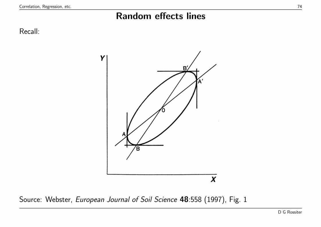
Correlation, Regression, etc. 74
Random effects lines
Recall:
Source: Webster, European Journal of Soil Science 48:558 (1997), Fig. 1
D G Rossiter
Correlation, Regression, etc. 75
Which equation is “correct”?
1. If modelling straw based on grain: regression straw vs. grain
2. If modelling grain based on straw: regression grain vs. straw
3. If modelling the relation between grain and straw: structural analysis
The relation is interesting e.g. for the best description of plant morphology: thegrain/straw ratio
D G Rossiter
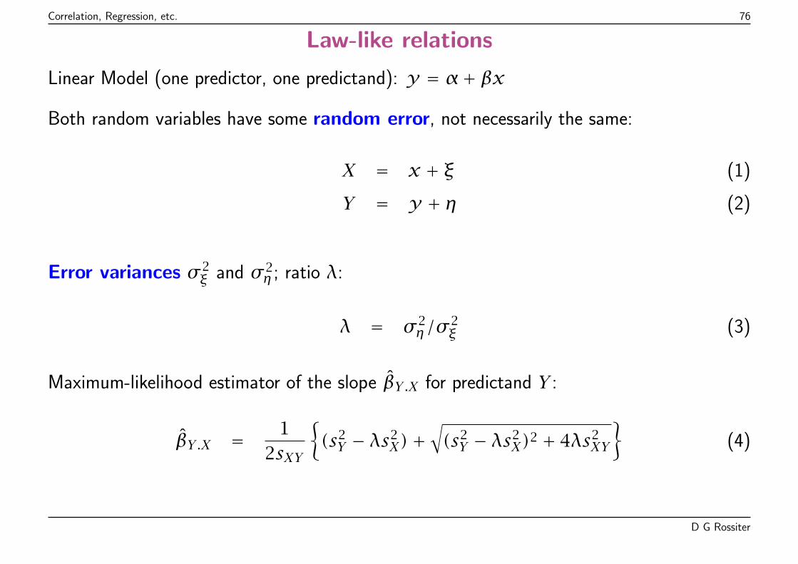
Correlation, Regression, etc. 76
Law-like relations
Linear Model (one predictor, one predictand): y = α+ βx
Both random variables have some random error, not necessarily the same:
X = x + ξ (1)
Y = y + η (2)
Error variances σ 2ξ and σ 2
η ; ratio λ:
λ = σ 2η/σ
2ξ (3)
Maximum-likelihood estimator of the slope βY .X for predictand Y :
βY .X = 12sXY
{(s2Y − λs2
X)+√(s2Y − λs2
X)2 + 4λs2XY
}(4)
D G Rossiter
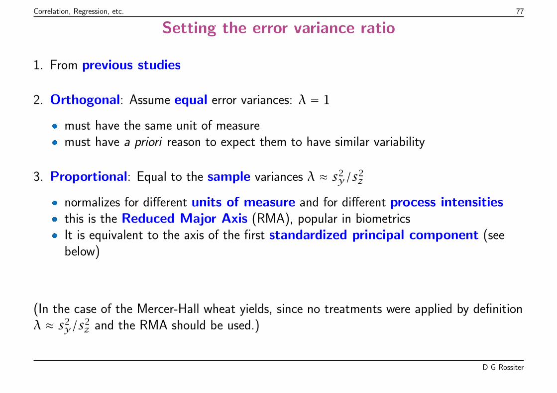
Correlation, Regression, etc. 77
Setting the error variance ratio
1. From previous studies
2. Orthogonal: Assume equal error variances: λ = 1
� must have the same unit of measure� must have a priori reason to expect them to have similar variability
3. Proportional: Equal to the sample variances λ ≈ s2y/s2
z
� normalizes for different units of measure and for different process intensities� this is the Reduced Major Axis (RMA), popular in biometrics� It is equivalent to the axis of the first standardized principal component (see
below)
(In the case of the Mercer-Hall wheat yields, since no treatments were applied by definitionλ ≈ s2
y/s2z and the RMA should be used.)
D G Rossiter
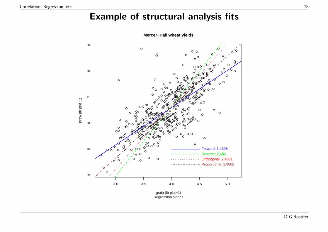
Correlation, Regression, etc. 78
Example of structural analysis fits
●
●
●
●
●
●
●
●
●
●●
● ●●
●
●
●
●
●
●
●
●
●
●
●
●
●
●
●
●●
●
●
●
●
●
●
●
●
●
●
●●
●
●
● ●●
●
●
●
●
●
●
●
●
●
●
●
●
●
●
●
●
●
●
●
●
●●
●
●
●
●
●
●
●
●
●●
●
●
●
●
●
●
●
●
●
●
●
●
● ●
●
●
●
●
●
●
●
●
●
●
●
●● ●
● ●
●
●
●
●
●
●
●
●
●
●
●
●
●
●
●
●
●
●
●
●
●
●
●
●
●
●
●●
●
●
●
●
●
●●
●
●
●
●
●
●●
●●
●
●
●
●
●
●
●●
●
●
●
●
●
●
●●
●
●●
●
●
●
●
●
●
●
●
●
●
●
●
●
●●
●
●● ●●
●
●
●
●
●
●
●
●
●●
●
●
●
●●
●
●
●
●
●
●
●
●
●
●
●
●
●
●●
●
●
●
●
●
●
●
●
●
●
●
●
●
●
●
●
●
●
●
●
●●
●
●
●
●
●
●
●
●
●
●
●
●
●
●
●
●
●
●
●
●
●●
●
●
●●
●
● ●
●
●
●
●
●
●
●
●
●
●
●
●
●
●
●
●
●●
●
●
●
●
●
●
●
● ●
●
●
●
●
●
●
●
●
●
●
●
●
●
●
●
●
●
●●
●
●
●
●
●
●
●
●
●
●
●
●
●
●
●
●
●
●
●
●
●
●
●
●
●
●
●
●
●
●●
●
●●
●
●
●
●
●
●
●
●
●
●
●
●
●
●
●
●
●
●
●
●
●●
● ●
●
●
●
●
●
●
●
●
●
●
●●
●
●
●
●
● ●●
●
●
●
●
●
●●
● ●
●
●
●
●
●
●
●
● ●
●
●●
●
●
●
●
●
●
●
●
●
●
●●
●●
●
●
●
●
●
● ●
●
●
●
●
●
●
●
●
●
●●
●
●
●
●
●
●
●●
●
●
●
●
●
●
●●
●
●
●
●
●
●
●●●
●
●
●
●
●
●
●
●
● ●
●
●
●
●
●
●
●
●
●
●
●
●
●
●
●
3.0 3.5 4.0 4.5 5.0
45
67
89
Mercer−Hall wheat yields
Regression slopesgrain (lb plot−1)
stra
w (
lb p
lot−
1)
Forward: 1.4305
Proportional: 1.9602Orthogonal: 2.4031Reverse: 2.686
D G Rossiter
Correlation, Regression, etc. 79
Topic: Multiple linear regression
Objective: model one variable (the predictand) from several other variables (thepredictors or explanatory variables)
� to“explain”
� to predict
D G Rossiter
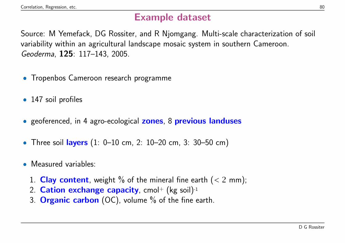
Correlation, Regression, etc. 80
Example dataset
Source: M Yemefack, DG Rossiter, and R Njomgang. Multi-scale characterization of soilvariability within an agricultural landscape mosaic system in southern Cameroon.Geoderma, 125: 117–143, 2005.
� Tropenbos Cameroon research programme
� 147 soil profiles
� geoferenced, in 4 agro-ecological zones, 8 previous landuses
� Three soil layers (1: 0–10 cm, 2: 10–20 cm, 3: 30–50 cm)
� Measured variables:
1. Clay content, weight % of the mineral fine earth (< 2 mm);2. Cation exchange capacity, cmol+ (kg soil)-1
3. Organic carbon (OC), volume % of the fine earth.
D G Rossiter
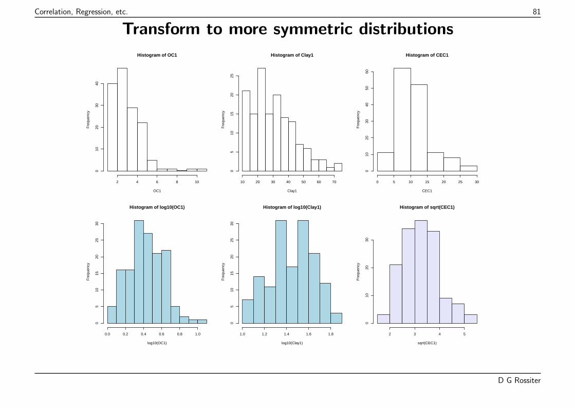
Correlation, Regression, etc. 81
Transform to more symmetric distributions
Histogram of OC1
OC1
Fre
quen
cy
2 4 6 8 10
010
2030
40
Histogram of Clay1
Clay1
Fre
quen
cy
10 20 30 40 50 60 70
05
1015
2025
Histogram of CEC1
CEC1
Fre
quen
cy
0 5 10 15 20 25 30
010
2030
4050
60
Histogram of log10(OC1)
log10(OC1)
Fre
quen
cy
0.0 0.2 0.4 0.6 0.8 1.0
05
1015
2025
30
Histogram of log10(Clay1)
log10(Clay1)
Fre
quen
cy
1.0 1.2 1.4 1.6 1.8
05
1015
2025
30
Histogram of sqrt(CEC1)
sqrt(CEC1)
Fre
quen
cy
2 3 4 5
010
2030
D G Rossiter
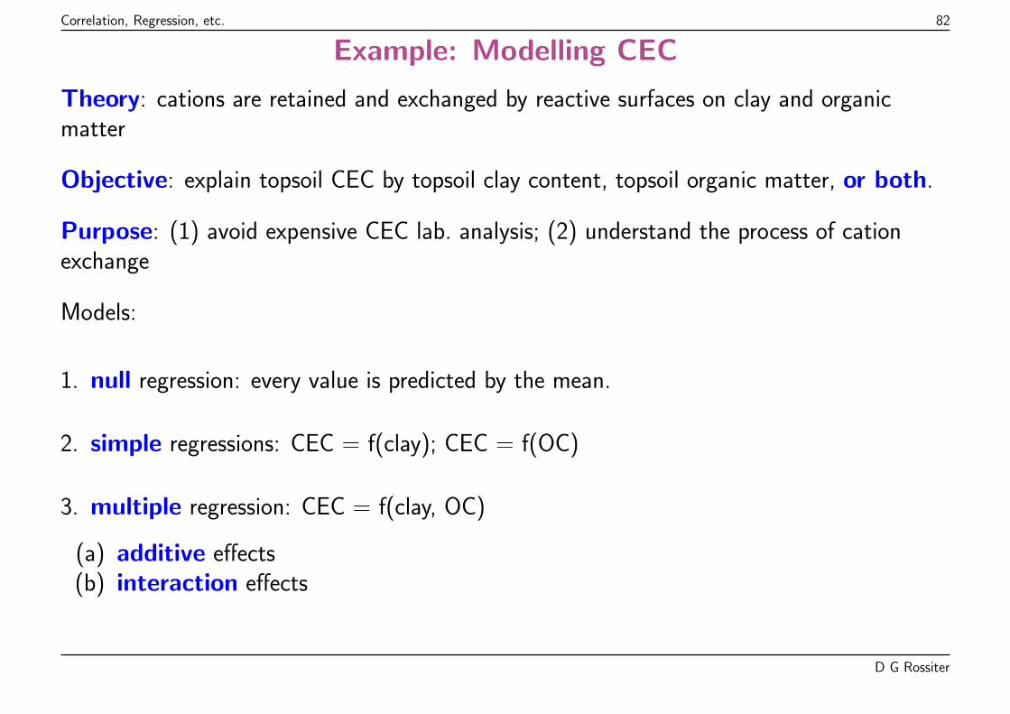
Correlation, Regression, etc. 82
Example: Modelling CEC
Theory: cations are retained and exchanged by reactive surfaces on clay and organicmatter
Objective: explain topsoil CEC by topsoil clay content, topsoil organic matter, or both.
Purpose: (1) avoid expensive CEC lab. analysis; (2) understand the process of cationexchange
Models:
1. null regression: every value is predicted by the mean.
2. simple regressions: CEC = f(clay); CEC = f(OC)
3. multiple regression: CEC = f(clay, OC)
(a) additive effects(b) interaction effects
D G Rossiter
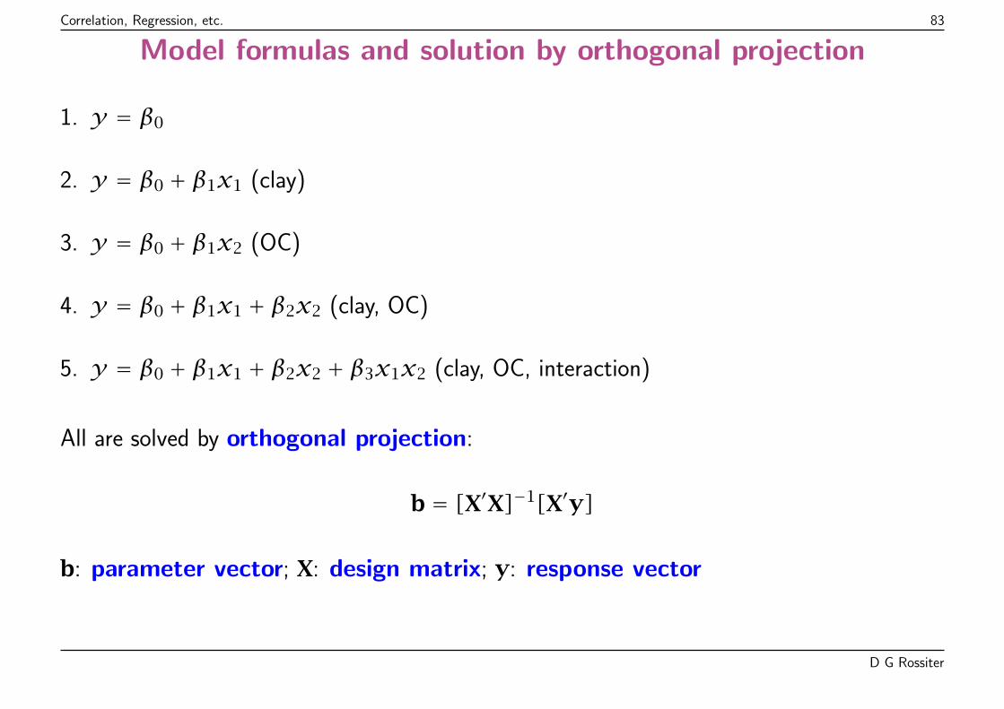
Correlation, Regression, etc. 83
Model formulas and solution by orthogonal projection
1. y = β0
2. y = β0 + β1x1 (clay)
3. y = β0 + β1x2 (OC)
4. y = β0 + β1x1 + β2x2 (clay, OC)
5. y = β0 + β1x1 + β2x2 + β3x1x2 (clay, OC, interaction)
All are solved by orthogonal projection:
b = [X′X]−1[X′y]
b: parameter vector; X: design matrix; y: response vector
D G Rossiter
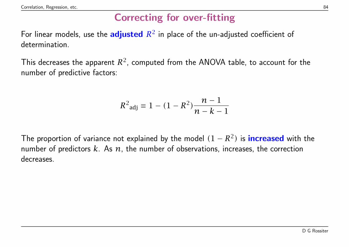
Correlation, Regression, etc. 84
Correcting for over-fitting
For linear models, use the adjusted R2 in place of the un-adjusted coefficient ofdetermination.
This decreases the apparent R2, computed from the ANOVA table, to account for thenumber of predictive factors:
R2adj ≡ 1− (1− R2)
n− 1n− k− 1
The proportion of variance not explained by the model (1− R2) is increased with thenumber of predictors k. As n, the number of observations, increases, the correctiondecreases.
D G Rossiter
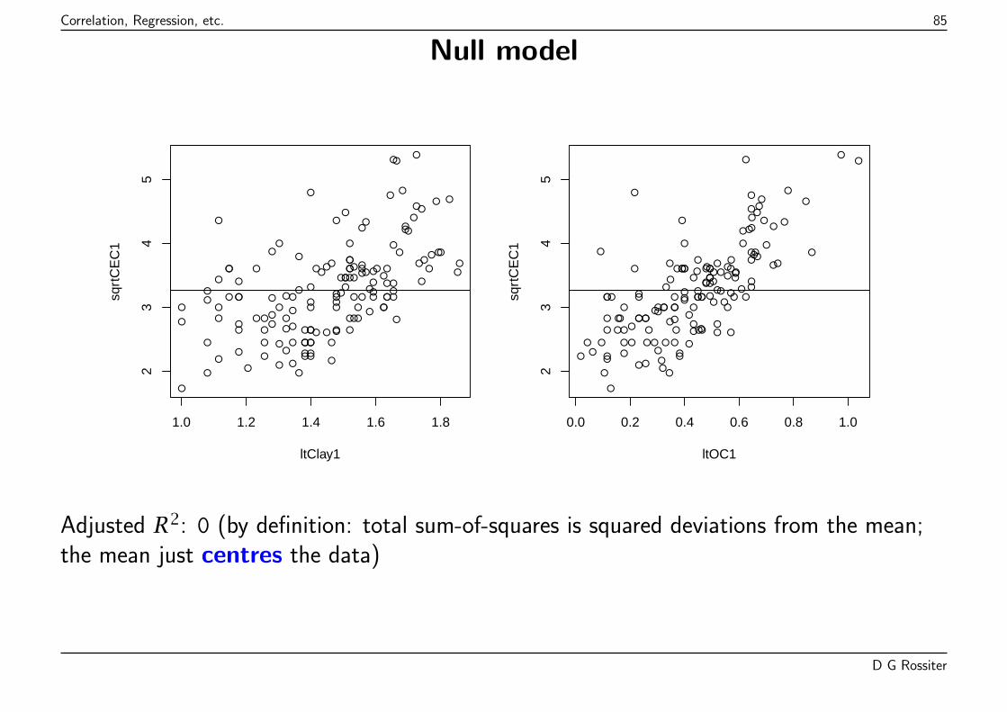
Correlation, Regression, etc. 85
Null model
●●
●
●
●
●
●●
●
●●
●
●
●
●
●
●
●●●
●
●
●
●●
●
●
●
●
●
●
●
●
●
●
●
●
●
●
●
●
●
●
●●
●
●
●
●●
●
●
●
●
●
●
●
●
●
●
●●
●
●
●●
●
●
●
●●
●
●
●
● ●
●
●
●
●●
●
●
●
●
●●
●
●
●
●
●
●●
●
●
●●●
●
●
●●
●
●
●
●
●
●
●
●
●
●●
●
●
●
●
●
●
●
●
●
●
●
●● ●
●
●
●
●
●
●
●
● ●
●
●
●
●
●
●
●
●
●
●
1.0 1.2 1.4 1.6 1.8
23
45
ltClay1
sqrt
CE
C1
●●
●
●
●
●
●●
●
●●
●
●
●
●
●
●
●●●
●
●
●
●●
●
●
●
●
●
●
●
●
●
●
●
●
●
●
●
●
●
●
●●
●
●
●
●●
●
●
●
●
●
●
●
●
●
●
●●
●
●
●●
●
●
●
●●
●
●
●
●●
●
●
●
● ●
●
●
●
●
● ●
●
●
●
●
●
●●
●
●
●●●
●
●
●●
●
●
●
●
●
●
●
●
●
●●
●
●
●
●
●
●
●
●
●
●
●
●●●
●
●
●
●
●
●
●
● ●
●
●
●
●
●
●
●
●
●
●
0.0 0.2 0.4 0.6 0.8 1.0
23
45
ltOC1
sqrt
CE
C1
Adjusted R2: 0 (by definition: total sum-of-squares is squared deviations from the mean;the mean just centres the data)
D G Rossiter
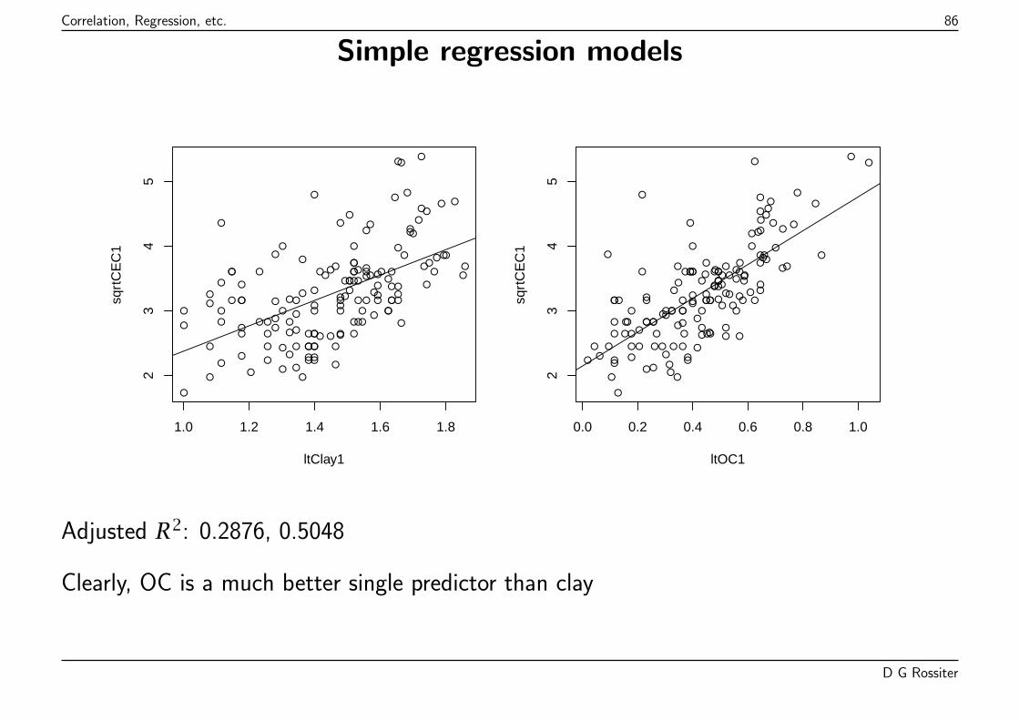
Correlation, Regression, etc. 86
Simple regression models
●●
●
●
●
●
●●
●
●●
●
●
●
●
●
●
●●●
●
●
●
●●
●
●
●
●
●
●
●
●
●
●
●
●
●
●
●
●
●
●
●●
●
●
●
●●
●
●
●
●
●
●
●
●
●
●
●●
●
●
●●
●
●
●
●●
●
●
●
● ●
●
●
●
●●
●
●
●
●
●●
●
●
●
●
●
●●
●
●
●●●
●
●
●●
●
●
●
●
●
●
●
●
●
●●
●
●
●
●
●
●
●
●
●
●
●
●● ●
●
●
●
●
●
●
●
● ●
●
●
●
●
●
●
●
●
●
●
1.0 1.2 1.4 1.6 1.8
23
45
ltClay1
sqrt
CE
C1
●●
●
●
●
●
●●
●
●●
●
●
●
●
●
●
●●●
●
●
●
●●
●
●
●
●
●
●
●
●
●
●
●
●
●
●
●
●
●
●
●●
●
●
●
●●
●
●
●
●
●
●
●
●
●
●
●●
●
●
●●
●
●
●
●●
●
●
●
●●
●
●
●
● ●
●
●
●
●
● ●
●
●
●
●
●
●●
●
●
●●●
●
●
●●
●
●
●
●
●
●
●
●
●
●●
●
●
●
●
●
●
●
●
●
●
●
●●●
●
●
●
●
●
●
●
● ●
●
●
●
●
●
●
●
●
●
●
0.0 0.2 0.4 0.6 0.8 1.0
23
45
ltOC1
sqrt
CE
C1
Adjusted R2: 0.2876, 0.5048
Clearly, OC is a much better single predictor than clay
D G Rossiter
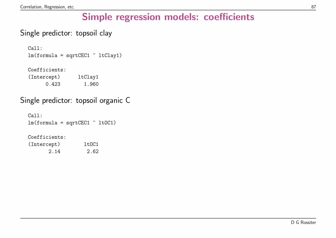
Correlation, Regression, etc. 87
Simple regression models: coefficients
Single predictor: topsoil clay
Call:
lm(formula = sqrtCEC1 ~ ltClay1)
Coefficients:
(Intercept) ltClay1
0.423 1.960
Single predictor: topsoil organic C
Call:
lm(formula = sqrtCEC1 ~ ltOC1)
Coefficients:
(Intercept) ltOC1
2.14 2.62
D G Rossiter
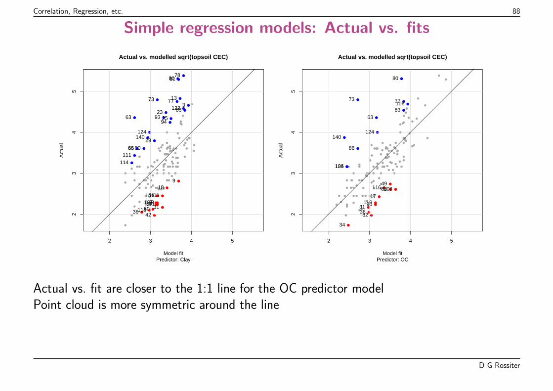
Correlation, Regression, etc. 88
Simple regression models: Actual vs. fits
●
●
●
●
●
●
●●
●
●
●
●
●
●
●
●
●
●●●
●
●
●
●
●
●
●
●
●
●
●
●
●
●
●
●
●
●
●
●
●
●
●
●
●
●
●
●
●
●
●
●
●
●
●
●
●
●
●
●
●●
●
●
●●
●
●
●
●
●
●
●
●
● ●
●
●
●
●●
●
●
●
●
●●
●
●
●
●
●
●
●
●
●
●●
●
●
●
●
●●
●
●
●
●
●
●
●
●
●
●
●
●
●
●
●
●
●
●
●
●
●
●
● ●
●
●
●
●
●
●
●
● ●
●
●
●
●
●
●
●
●
●
●
2 3 4 5
23
45
Model fit
Act
ual
Actual vs. modelled sqrt(topsoil CEC)
Predictor: Clay
3
9
13
18
2325
27
29
3136
42
51
60
63
6566
73 77
788081
83
90
9394
96
100107110
111114
118
122
124140
144
●
●
●
●
●
●
●●
●
●
●
●
●
●
●
●
●
●●●
●
●
●
●
●
●
●
●
●
●
●
●
●
●
●
●
●
●
●
●
●
●
●
●
●
●
●
●
●
●
●
●
●
●
●
●
●
●
●
●
●●
●
●
●●
●
●
●
●
●
●
●
●
●●
●
●
●
● ●
●
●
●
●
● ●
●
●
●
●
●
●
●
●
●
●●
●
●
●
●
●
●
●
●
●
●
●
●
●
●
●
●
●
●
●
●
●
●
●
●
●
●
●
●
●●
●
●
●
●
●
●
●
● ●
●
●
●
●
●
●
●
●
●
●
2 3 4 5
23
45
Model fit
Act
ual
Actual vs. modelled sqrt(topsoil CEC)
Predictor: OC
17
31
34
36
49
63
73 77
80
82
83
86
88
96
104
106
108
110
116
124
135
140
Actual vs. fit are closer to the 1:1 line for the OC predictor modelPoint cloud is more symmetric around the line
D G Rossiter
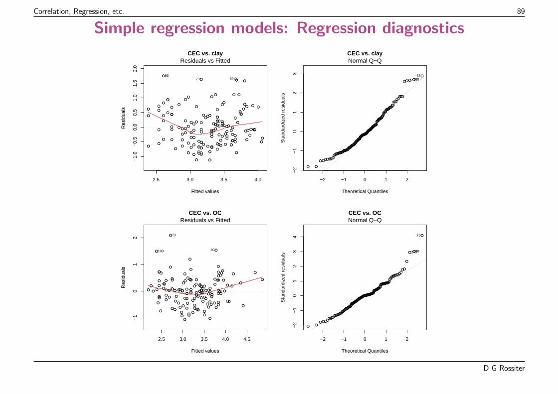
Correlation, Regression, etc. 89
Simple regression models: Regression diagnostics
2.5 3.0 3.5 4.0
−1.
0−
0.5
0.0
0.5
1.0
1.5
2.0
CEC vs. clay
Fitted values
Res
idua
ls
●
●
●
●
●
●
●●
●
●
●
●
●
●
●
●
●
●
●●
●
●
●
●
●
●
●
●
●
●
●
●●
●
●
●
●
●
● ●
●
●
●
●
●
●
●
●●
●
●
●●
●
●
●
●
●
●
●
●●
●
●
●●
●
●
●
●● ●
●
●
●●
●
●
●
●●
●
●
●
●
●●
●
●
●
●
●
●
●
●
●
●
●
●
●
●
●
●
●
●
●
●
●
●
●
●
●
●
●
●
●
●
●
●
●
●
●
●
●
●
●
●
●
●
●
●● ●
●
●
●
●
●
●
●
●
●
●
● ●
●
●
Residuals vs Fitted
638073
●
●
●
●
●
●
●●
●
●
●
●
●
●
●
●
●
●
●●
●
●
●
●
●
●
●
●
●
●
●
●●
●
●
●
●
●
●●
●
●
●
●
●
●
●
●
●
●
●
●
●
●
●
●
●
●
●
●
●●
●
●
●●
●
●
●
●●●
●
●
●●
●
●
●
●●
●
●
●
●
●●
●
●
●
●
●
●
●
●
●
●
●
●
●
●
●
●
●
●
●
●
●
●
●
●
●
●
●
●
●
●
●
●
●
●
●
●
●
●
●
●
●
●
●
●●●
●
●
●
●
●
●
●
●
●
●
● ●
●
●
−2 −1 0 1 2
−2
−1
01
23
CEC vs. clay
Theoretical Quantiles
Sta
ndar
dize
d re
sidu
als
Normal Q−Q
638073
2.5 3.0 3.5 4.0 4.5
−1
01
2
CEC vs. OC
Fitted values
Res
idua
ls
●
●
●
●●
●
●●
●
●
●
●
●
●
●
●
●●●
● ●●
●
●
●
●
●
●
●●
●
●
●
●
●
●
●● ●
●●
● ●
●
●
●
●
●
●
●
●
● ●●
●
●
●
●
●
●
●●
●
●
●●
●
●
●
●
● ●
●
●
●●
●
●
●
●
●
●
●
●
●
●
●
●
●
●
●
●
●●
●
●
●
●
●●
●●
●
●
●
●
●
●
●
●
●
●
●●
●●
●
● ●
●
●
●
●
●
●
●
●●
●● ●
●
● ●
●
●●
●
●
●
●
●
●
●
● ●
●
Residuals vs Fitted
73
80140
●
●
●
●●
●
●●
●
●
●
●
●
●
●
●
●●●
●●●
●
●
●
●
●
●
●●
●
●
●
●
●
●
●●●
●●
●●
●
●
●
●
●
●
●
●
●●●
●
●
●
●
●
●
●●
●
●
●●
●
●
●
●
●●
●
●
●●
●
●
●
●
●
●
●
●
●
●
●
●
●
●
●
●
●●
●
●
●
●
●●
●●
●
●
●
●
●
●
●
●
●
●
●●
●●
●
● ●
●
●
●
●
●
●
●
●●
●●●
●
●●
●
●●
●
●
●
●
●
●
●
●●
●
−2 −1 0 1 2
−2
−1
01
23
4
CEC vs. OC
Theoretical Quantiles
Sta
ndar
dize
d re
sidu
als
Normal Q−Q
73
80140
D G Rossiter
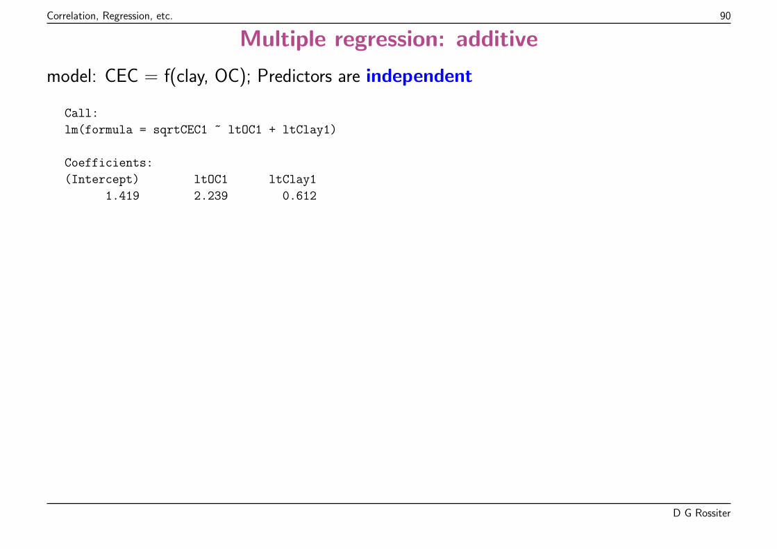
Correlation, Regression, etc. 90
Multiple regression: additive
model: CEC = f(clay, OC); Predictors are independent
Call:
lm(formula = sqrtCEC1 ~ ltOC1 + ltClay1)
Coefficients:
(Intercept) ltOC1 ltClay1
1.419 2.239 0.612
D G Rossiter
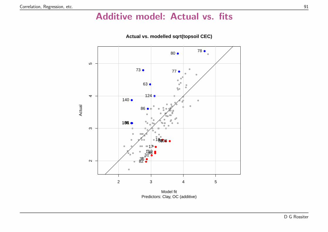
Correlation, Regression, etc. 91
Additive model: Actual vs. fits
●
●
●
●
●
●
●●
●
●
●
●
●
●
●
●
●
●●●
●
●
●
●
●
●
●
●
●
●
●
●
●
●
●
●
●
●
●
●
●
●
●
●
●
●
●
●
●
●
●
●
●
●
●
●
●
●
●
●
●●
●
●
●●
●
●
●
●
●
●
●
●
●●
●
●
●
● ●
●
●
●
●
● ●
●
●
●
●
●
●
●
●
●
●●
●
●
●
●
●
●
●
●
●
●
●
●
●
●
●
●
●
●
●
●
●
●
●
●
●
●
●
●
● ●
●
●
●
●
●
●
●
● ●
●
●
●
●
●
●
●
●
●
●
2 3 4 5
23
45
Model fit
Act
ual
Actual vs. modelled sqrt(topsoil CEC)
Predictors: Clay, OC (additive)
17
18
3136
63
73 77
7880
82
86
88
91
96
104
108
110
124
135
140
D G Rossiter
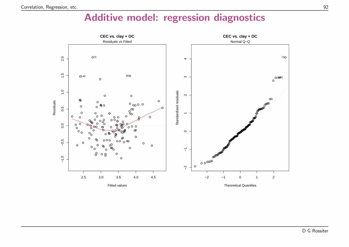
Correlation, Regression, etc. 92
Additive model: regression diagnostics
2.5 3.0 3.5 4.0 4.5
−1.
0−
0.5
0.0
0.5
1.0
1.5
2.0
CEC vs. clay + OC
Fitted values
Res
idua
ls
●
●
●
●
●
●
●●
●
●
●
●
●
●
●
●
● ●
●
●●
●
●
●
●
●
●
●
●
●
●
●
●
●
●
●
●●
●
●
●
●
●
●
●
●
●
●
●
●
●
● ●
●
●
●
●
●
●
●
●●
●
●
●●
●
●●
●
●●
●
●
●●
●
●
●
●
●
●
●
● ●
●
●
●
●
●
●
●
●●
●
●
●
●
●
●
●●
●
●
●
●
●
●
●
●
●
●
●
●
●●
●
●●
●
●
●
●
●
●
●
●●
●●●
●
●
●
●
●
●
●
●
●
●
●
●
●
●
●
●
Residuals vs Fitted
73
80140
●
●
●
●
●
●
●●
●
●
●
●
●
●
●
●
●●
●
●●
●
●
●
●
●
●
●
●
●
●
●
●
●
●
●
●●
●
●
●
●
●
●
●
●
●
●
●
●
●
●●
●
●
●
●
●
●
●
●●
●
●
●●
●
●●
●
●●
●
●
●●
●
●
●
●
●
●
●
●●
●
●
●
●
●
●
●
●●
●
●
●
●
●
●
●●
●
●
●
●
●
●
●
●
●
●
●
●
●●
●
●●
●
●
●
●
●
●
●
●
●
●●●
●
●
●
●
●
●
●
●
●
●
●
●
●
●
●
●
−2 −1 0 1 2
−2
−1
01
23
4
CEC vs. clay + OC
Theoretical Quantiles
Sta
ndar
dize
d re
sidu
als
Normal Q−Q
73
80140
D G Rossiter
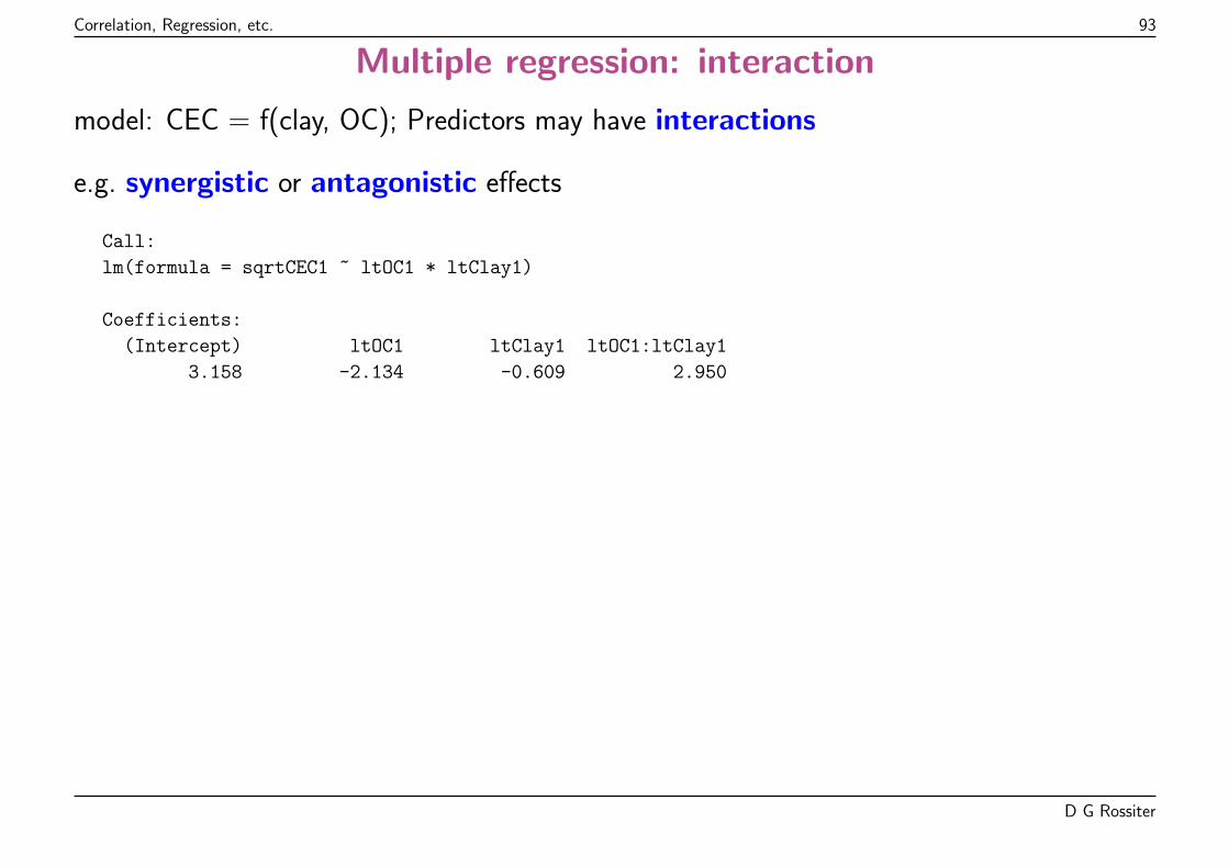
Correlation, Regression, etc. 93
Multiple regression: interaction
model: CEC = f(clay, OC); Predictors may have interactions
e.g. synergistic or antagonistic effects
Call:
lm(formula = sqrtCEC1 ~ ltOC1 * ltClay1)
Coefficients:
(Intercept) ltOC1 ltClay1 ltOC1:ltClay1
3.158 -2.134 -0.609 2.950
D G Rossiter
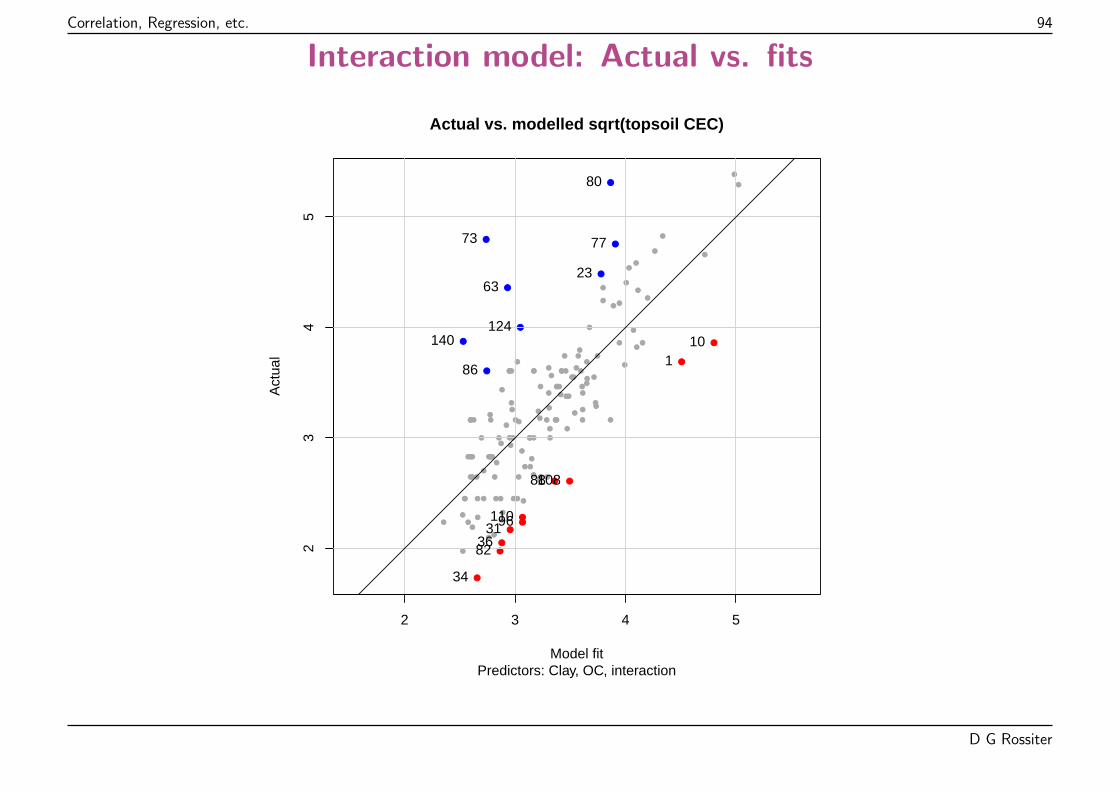
Correlation, Regression, etc. 94
Interaction model: Actual vs. fits
●
●
●
●
●
●
●●
●
●
●
●
●
●
●
●
●
●●●
●
●
●
●
●
●
●
●
●
●
●
●
●
●
●
●
●
●
●
●
●
●
●
●
●
●
●
●
●
●
●
●
●
●
●
●
●
●
●
●
●●
●
●
●●
●
●
●
●
●
●
●
●
●●
●
●
●
● ●
●
●
●
●
● ●
●
●
●
●
●
●
●
●
●
●●
●
●
●
●
●●
●
●
●
●
●
●
●
●
●
●
●
●
●
●
●
●
●
●
●
●
●
●
●●
●
●
●
●
●
●
●
● ●
●
●
●
●
●
●
●
●
●
●
2 3 4 5
23
45
Model fit
Act
ual
Actual vs. modelled sqrt(topsoil CEC)
Predictors: Clay, OC, interaction
110
23
31
34
36
63
73 77
80
82
86
88
96
108
110
124140
D G Rossiter
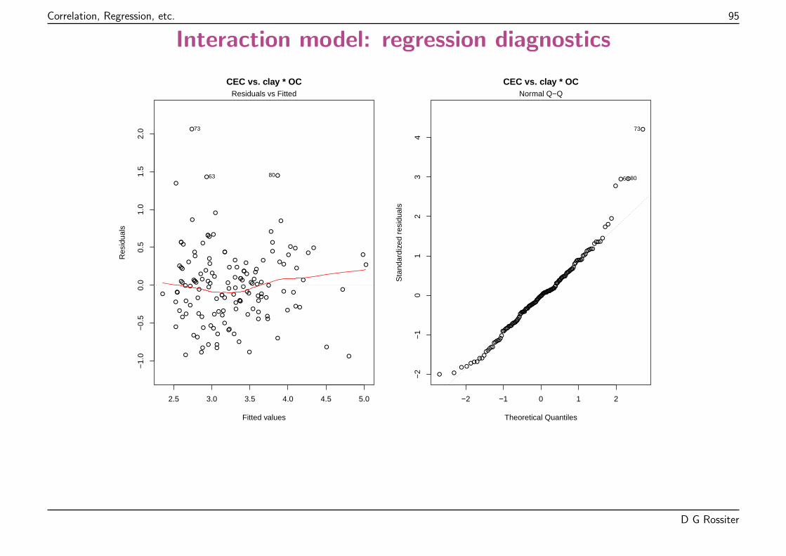
Correlation, Regression, etc. 95
Interaction model: regression diagnostics
2.5 3.0 3.5 4.0 4.5 5.0
−1.
0−
0.5
0.0
0.5
1.0
1.5
2.0
CEC vs. clay * OC
Fitted values
Res
idua
ls
●
●
●
●
●
●
●●●
●
●●
●
●
●
●
● ●
●
●
●
●
●
●●
●●
●
●
●
●
●
●
●
●
●
●
●
●
●
●
●
●
●
●
●
●
●
●
●
●
● ● ●
●
●
●
●
●
●
●●
●
●
●●
●
●
●
●
●●
●
●
●●
●
●
●
●
●
●
●
●
●
●
●
●
●
●
●
●
●
●
●
●
●
●
●
●
●●
●
●
●
●
●
●
●
●
●
●
●
●
● ●
●
●
●
●
●
●
●
●
●
●
●●
●●
●●
●●
●
●
●
●
●
●
●
●
●
●
●
●
●
Residuals vs Fitted
73
8063
●
●
●
●
●
●
●●●
●
●●
●
●
●
●
●●
●
●
●
●
●
●●
●●
●
●
●
●
●
●
●
●
●
●
●
●
●
●
●
●
●
●
●
●
●
●
●
●
●●●
●
●
●
●
●
●
●●
●
●
●●
●
●
●
●
●●
●
●
●●
●
●
●
●
●
●
●
●
●
●
●
●
●
●
●
●
●
●
●
●
●
●
●
●
●●
●
●
●
●
●
●
●
●
●
●
●
●
●●
●
●
●
●
●
●
●
●
●
●
●●
●●
●●
●●
●
●
●
●
●
●
●
●
●
●
●
●
●
−2 −1 0 1 2
−2
−1
01
23
4
CEC vs. clay * OC
Theoretical Quantiles
Sta
ndar
dize
d re
sidu
als
Normal Q−Q
73
8063
D G Rossiter
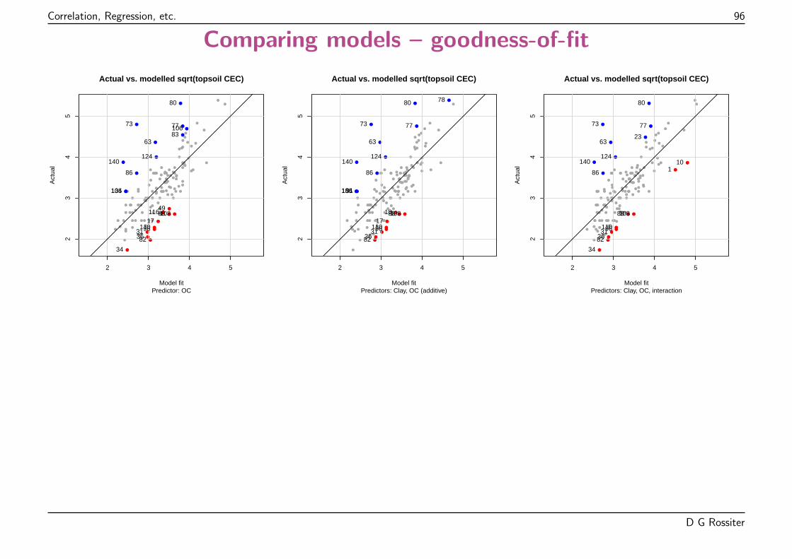
Correlation, Regression, etc. 96
Comparing models – goodness-of-fit
●
●
●
●
●
●
●●
●
●
●
●
●
●
●
●
●
●●●
●
●
●
●
●
●
●
●
●
●
●
●
●
●
●
●
●
●
●
●
●
●
●
●
●
●
●
●
●●
●
●
●
●
●
●
●
●
●
●
●●
●
●
●●
●
●
●
●
●
●
●
●
●●
●
●
●
● ●
●
●
●
●
● ●
●
●
●
●
●
●
●
●
●
●●
●
●
●
●
●●
●
●
●
●
●
●
●
●
●
●
●
●
●
●
●
●
●
●
●
●
●
●
●●
●
●
●
●
●
●
●
● ●
●
●
●
●
●
●
●
●
●
●
2 3 4 5
23
45
Model fit
Act
ual
Actual vs. modelled sqrt(topsoil CEC)
Predictor: OC
17
31
34
36
49
63
73 77
80
82
83
86
88
96
104
106
108
110
116
124
135
140●
●
●
●
●
●
●●
●
●
●
●
●
●
●
●
●
●●●
●
●
●
●
●
●
●
●
●
●
●
●
●
●
●
●
●
●
●
●
●
●
●
●
●
●
●
●
●
●
●
●
●
●
●
●
●
●
●
●
●●
●
●
●●
●
●
●
●
●
●
●
●
●●
●
●
●
● ●
●
●
●
●
● ●
●
●
●
●
●
●
●
●
●
●●
●
●
●
●
●●
●
●
●
●
●
●
●
●
●
●
●
●
●
●
●
●
●
●
●
●
●
●
● ●
●
●
●
●
●
●
●
● ●
●
●
●
●
●
●
●
●
●
●
2 3 4 5
23
45
Model fitA
ctua
l
Actual vs. modelled sqrt(topsoil CEC)
Predictors: Clay, OC (additive)
1718
3136
63
73 77
7880
82
86
88
91
96
104
108
110
124
135
140●
●
●
●
●
●
●●
●
●
●
●
●
●
●
●
●
●●●
●
●
●
●
●
●
●
●
●
●
●
●
●
●
●
●
●
●
●
●
●
●
●
●
●
●
●
●
●
●
●
●
●
●
●
●
●
●
●
●
●●
●
●
●●
●
●
●
●
●
●
●
●
●●
●
●
●
● ●
●
●
●
●
● ●
●
●
●
●
●
●
●
●
●
●●
●
●
●
●
●●
●
●
●
●
●
●
●
●
●
●
●
●
●
●
●
●
●
●
●
●
●
●
●●
●
●
●
●
●
●
●
● ●
●
●
●
●
●
●
●
●
●
●
2 3 4 5
23
45
Model fit
Act
ual
Actual vs. modelled sqrt(topsoil CEC)
Predictors: Clay, OC, interaction
110
23
31
34
36
63
73 77
80
82
86
88
96
108
110
124140
D G Rossiter
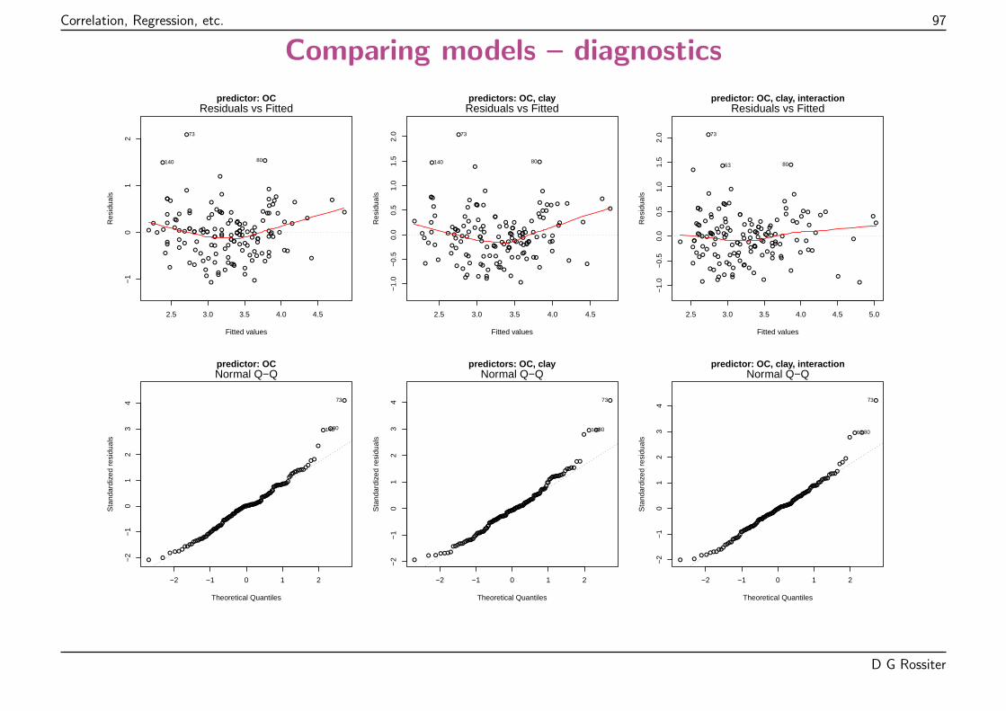
Correlation, Regression, etc. 97
Comparing models – diagnostics
2.5 3.0 3.5 4.0 4.5
−1
01
2
predictor: OC
Fitted values
Res
idua
ls
●
●
●
●●
●
●●
●
●
●
●
●
●
●
●
●
●●
●●●
●
●
●
●
●
●
●●
●
●
●
●
●
●
●● ●
●●
● ●
●
●
●
●
●
●
●
●
● ●
●
●
●
●
●
●
●
●●
●
●
●●
●
●
●
●
● ●
●
●
●●
●
●
●
●
●
●
●
●
●
●
●
●
●
●
●
●
●●
●
●
●
●
●●
●●
●
●
●
●
●
●
●
●
●
●
●●
●●
●
● ●
●
●
●
●
●
●
●
●●
●● ●
●
● ●
●
●●
●
●
●
●
●
●
●
● ●
●
Residuals vs Fitted
73
80140
2.5 3.0 3.5 4.0 4.5
−1.
0−
0.5
0.0
0.5
1.0
1.5
2.0
predictors: OC, clay
Fitted values
Res
idua
ls
●
●
●
●
●
●
●●
●
●
●
●
●
●
●
●
● ●
●
● ●
●
●
●●
●
●
●
●●
●
●
●
●
●
●
●●
●
●
●
●
●
●
●
●
●
●
●
●
●
● ●●
●
●
●
●
●
●
●●
●
●
●●
●
●●
●
● ●
●
●●●
●
●
●
●
●
●
●
● ●
●
●
●
●
●
●
●
●●
●
●
●
●
●
●
●●
●
●
●
●
●
●
●
●
●
●
●
●
● ●
●
●●
●
●
●
●
●
●
●
●●
●● ●
●●
●
●
●
●
●
●
●
●
●
●
●
●●
●
Residuals vs Fitted
73
80140
2.5 3.0 3.5 4.0 4.5 5.0
−1.
0−
0.5
0.0
0.5
1.0
1.5
2.0
predictor: OC, clay, interaction
Fitted values
Res
idua
ls
●
●●
●
●
●
●●●
●
●●
●
●
●
●
● ●
●
●
●
●
●
●●
●●
●
●
●
●
●
●
●
●
●
●
●
●
●
●
●
●
●
●
●
●
●
●
●
●
● ● ●
●
●
●
●
●
●
●●
●
●
●●
●
●
●
●
●●
●
●
●●
●
●●
●
●
●
●
●
●
●
●
●
●
●●
●
●
●
●
●
●
●
●
●
●●
●
●
●
●
●
●
●
●
●
●●
●
● ●
●
●●
●
●
●
●
●
●
●
●●
●●
●●
●●
●
●
●
●
●
●
●
●
●
●
●●
●
Residuals vs Fitted
73
8063
●
●
●
●●
●
●●
●
●
●
●
●
●
●
●
●
●●
●●●
●
●
●
●
●
●
●●
●
●
●
●
●
●
●●●
●●
●●
●
●
●
●
●
●
●
●
●●
●
●
●
●
●
●
●
●●
●
●
●●
●
●
●
●
●●
●
●
●●
●
●
●
●
●
●
●
●
●
●
●
●
●
●
●
●
●●
●
●
●
●
●●
●●
●
●
●
●
●
●
●
●
●
●
●●
●●
●
● ●
●
●
●
●
●
●
●
●●
●●●
●
●●
●
●●
●
●
●
●
●
●
●
●●
●
−2 −1 0 1 2
−2
−1
01
23
4
predictor: OC
Theoretical Quantiles
Sta
ndar
dize
d re
sidu
als
Normal Q−Q
73
80140
●
●
●
●
●
●
●●
●
●
●
●
●
●
●
●
●●
●
●●
●
●
●●
●
●
●
●
●
●
●
●
●
●
●
●●
●
●
●
●
●
●
●
●
●
●
●
●
●
●●●
●
●
●
●
●
●
●●
●
●
●●
●
●●
●
●●
●
●●●
●
●
●
●
●
●
●
●●
●
●
●
●
●
●
●
●●
●
●
●
●
●
●
●●
●
●
●
●
●
●
●
●
●
●
●
●
●●
●
●●
●
●
●
●
●
●
●
●●
●●●
●
●
●
●
●
●
●
●
●
●
●
●
●
●●
●
−2 −1 0 1 2
−2
−1
01
23
4
predictors: OC, clay
Theoretical Quantiles
Sta
ndar
dize
d re
sidu
als
Normal Q−Q
73
80140
●
●
●
●
●
●
●●●
●
●●
●
●
●
●
●●
●
●
●
●
●
●●
●●
●
●
●
●
●
●
●
●
●
●
●
●
●
●
●
●
●
●
●
●
●
●
●
●
●●●
●
●
●
●
●
●
●●
●
●
●●
●
●
●
●
●●
●
●
●●
●
●
●
●
●
●
●
●
●
●
●
●
●
●●
●
●
●
●
●
●
●
●
●
●●
●
●
●
●
●
●
●
●
●
●●
●
●●
●
●●
●
●
●
●
●
●
●
●●
●●
●●
●●
●
●
●
●
●
●
●
●
●
●
●●
●
−2 −1 0 1 2
−2
−1
01
23
4
predictor: OC, clay, interaction
Theoretical Quantiles
Sta
ndar
dize
d re
sidu
als
Normal Q−Q
73
8063
D G Rossiter
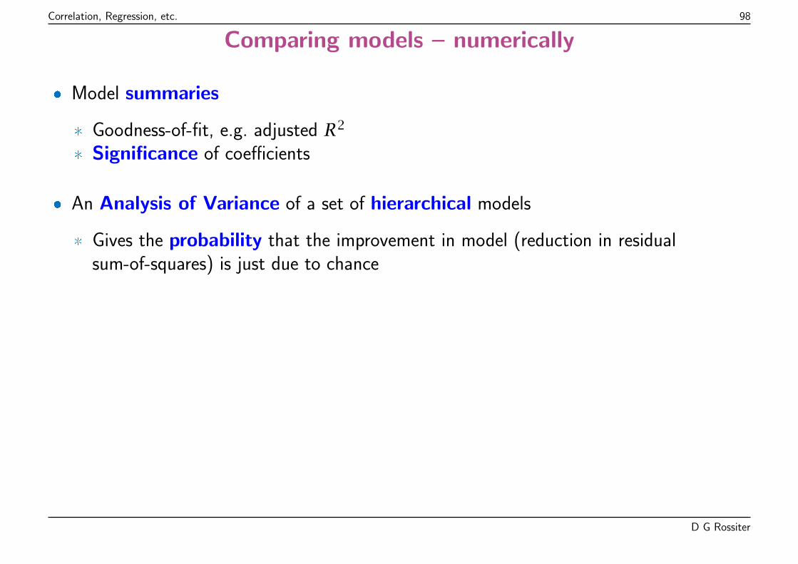
Correlation, Regression, etc. 98
Comparing models – numerically
� Model summaries
* Goodness-of-fit, e.g. adjusted R2
* Significance of coefficients
� An Analysis of Variance of a set of hierarchical models
* Gives the probability that the improvement in model (reduction in residualsum-of-squares) is just due to chance
D G Rossiter
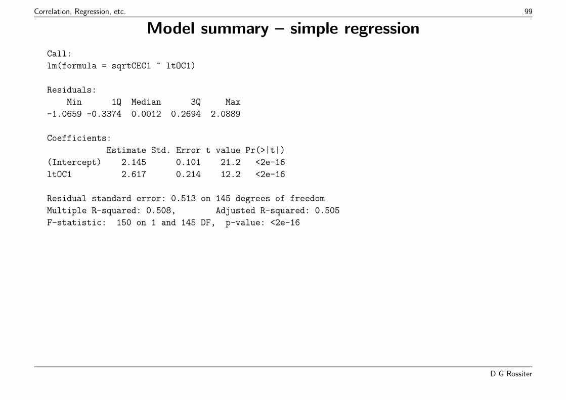
Correlation, Regression, etc. 99
Model summary – simple regression
Call:
lm(formula = sqrtCEC1 ~ ltOC1)
Residuals:
Min 1Q Median 3Q Max
-1.0659 -0.3374 0.0012 0.2694 2.0889
Coefficients:
Estimate Std. Error t value Pr(>|t|)
(Intercept) 2.145 0.101 21.2 <2e-16
ltOC1 2.617 0.214 12.2 <2e-16
Residual standard error: 0.513 on 145 degrees of freedom
Multiple R-squared: 0.508, Adjusted R-squared: 0.505
F-statistic: 150 on 1 and 145 DF, p-value: <2e-16
D G Rossiter
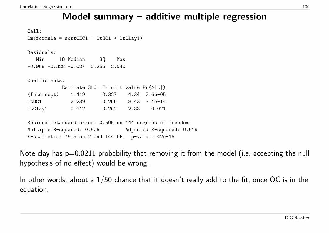
Correlation, Regression, etc. 100
Model summary – additive multiple regression
Call:
lm(formula = sqrtCEC1 ~ ltOC1 + ltClay1)
Residuals:
Min 1Q Median 3Q Max
-0.969 -0.328 -0.027 0.256 2.040
Coefficients:
Estimate Std. Error t value Pr(>|t|)
(Intercept) 1.419 0.327 4.34 2.6e-05
ltOC1 2.239 0.266 8.43 3.4e-14
ltClay1 0.612 0.262 2.33 0.021
Residual standard error: 0.505 on 144 degrees of freedom
Multiple R-squared: 0.526, Adjusted R-squared: 0.519
F-statistic: 79.9 on 2 and 144 DF, p-value: <2e-16
Note clay has p=0.0211 probability that removing it from the model (i.e. accepting the nullhypothesis of no effect) would be wrong.
In other words, about a 1/50 chance that it doesn’t really add to the fit, once OC is in theequation.
D G Rossiter
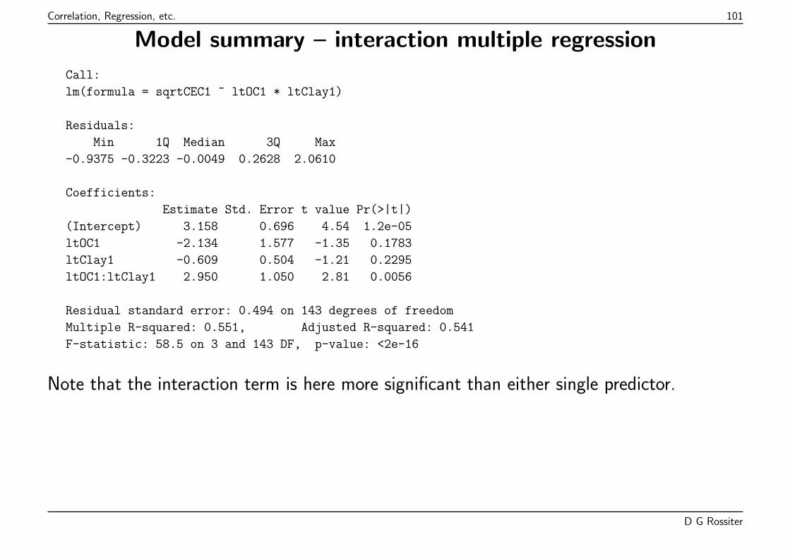
Correlation, Regression, etc. 101
Model summary – interaction multiple regression
Call:
lm(formula = sqrtCEC1 ~ ltOC1 * ltClay1)
Residuals:
Min 1Q Median 3Q Max
-0.9375 -0.3223 -0.0049 0.2628 2.0610
Coefficients:
Estimate Std. Error t value Pr(>|t|)
(Intercept) 3.158 0.696 4.54 1.2e-05
ltOC1 -2.134 1.577 -1.35 0.1783
ltClay1 -0.609 0.504 -1.21 0.2295
ltOC1:ltClay1 2.950 1.050 2.81 0.0056
Residual standard error: 0.494 on 143 degrees of freedom
Multiple R-squared: 0.551, Adjusted R-squared: 0.541
F-statistic: 58.5 on 3 and 143 DF, p-value: <2e-16
Note that the interaction term is here more significant than either single predictor.
D G Rossiter
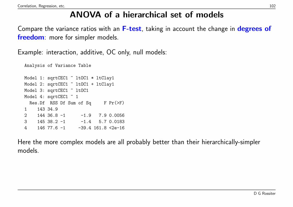
Correlation, Regression, etc. 102
ANOVA of a hierarchical set of models
Compare the variance ratios with an F-test, taking in account the change in degrees offreedom: more for simpler models.
Example: interaction, additive, OC only, null models:
Analysis of Variance Table
Model 1: sqrtCEC1 ~ ltOC1 * ltClay1
Model 2: sqrtCEC1 ~ ltOC1 + ltClay1
Model 3: sqrtCEC1 ~ ltOC1
Model 4: sqrtCEC1 ~ 1
Res.Df RSS Df Sum of Sq F Pr(>F)
1 143 34.9
2 144 36.8 -1 -1.9 7.9 0.0056
3 145 38.2 -1 -1.4 5.7 0.0183
4 146 77.6 -1 -39.4 161.8 <2e-16
Here the more complex models are all probably better than their hierarchically-simplermodels.
D G Rossiter
Correlation, Regression, etc. 103
Stepwise regression
Automatically decide which predictors to include
� Forward: start with best single-predictor model, keep adding predictors if they“significantly” improve model
� Backward: start with saturated model (all predictors, all interactions), keep deletingpredictors if the reduced model is not “significantly” worse
Comparing models: goodness-of-fit, adjusted for number of parameters
Problem: if there is (near)colinearity selection of predictors can be sensitive to just a fewdata points
Problem: can substitute for modeller’s judgement, especially if several models givesimilar results
D G Rossiter
Correlation, Regression, etc. 104
Example of stepwise regression
Predict CEC in the 30-50 cm layer . . .
. . . from all three variables (clay, OC, and CEC) for the two shallower layers
i.e. total of six possible predictors – are all necessary?
(Purpose: avoid sampling the deeper subsoil)
D G Rossiter
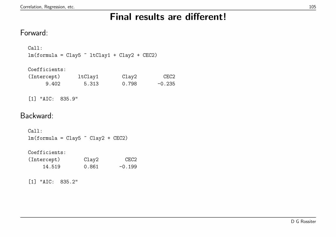
Correlation, Regression, etc. 105
Final results are different!
Forward:
Call:
lm(formula = Clay5 ~ ltClay1 + Clay2 + CEC2)
Coefficients:
(Intercept) ltClay1 Clay2 CEC2
9.402 5.313 0.798 -0.235
[1] "AIC: 835.9"
Backward:
Call:
lm(formula = Clay5 ~ Clay2 + CEC2)
Coefficients:
(Intercept) Clay2 CEC2
14.519 0.861 -0.199
[1] "AIC: 835.2"
D G Rossiter
Correlation, Regression, etc. 106
Topic: Regression trees
Objective: model one variable (the predictand) from several other variables (thepredictors or explanatory variables)
This is the same objective as for MLR and other model-based regression methods, but:
� no need to choose the functional form (e.g., multivariate linear)
� no assumption that the functional form is the same throughout the range of thepredictors.
� no need to transform predictors or predictand to satisfy the assumptions of a model form
� no need to choose among correlated predictor variables
� no need to explicitly consider (or not) interactions
D G Rossiter
Correlation, Regression, etc. 107
Data mining vs. statistical modelling
This is a data mining approach: do not impose a statistical model, rather, propose analgorithm to reveal the structure in the dataset.
Here the structure is a binary tree such that each split improves the prediction:
� by the maximum reduction in within-group variance
� this is equivalent to the maximum increase in between-group variance.
The leaves (terminal nodes) each then have a simple prediction model, usually aconstant that is the predicted value for all cases that end at that terminal node..
The tree can easily be interpreted: we see the variables and their threshold values, andcan follow the tree for any new observation. .
D G Rossiter
Correlation, Regression, etc. 108
Regression trees algorithm
1. Identify the predictors and predictand; compute the overall mean and variance of thepredictand.
2. Recursively:
(a) Look for the predictor variable, and its threshold value, that “best” splits thedata into two groups.� “Best”: maximum reduction in sum of within-group sums of squares in the response
variable: SST − (SSL + SSR).(b) Split at that point into two subtrees(c) Compute the mean and variance of the predictand in each group
3. This continues until the subgroups either:
(a) reach a user-specified minimum size, or(b) no substantial improvement can be made; that is the sum of the within-groups
sum of squares can not be further reduced below a user-defined threshold.
D G Rossiter
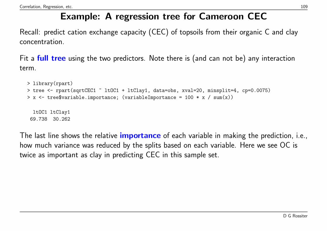
Correlation, Regression, etc. 109
Example: A regression tree for Cameroon CEC
Recall: predict cation exchange capacity (CEC) of topsoils from their organic C and clayconcentration.
Fit a full tree using the two predictors. Note there is (and can not be) any interactionterm.
> library(rpart)
> tree <- rpart(sqrtCEC1 ~ ltOC1 + ltClay1, data=obs, xval=20, minsplit=4, cp=0.0075)
> x <- tree$variable.importance; (variableImportance = 100 * x / sum(x))
ltOC1 ltClay1
69.738 30.262
The last line shows the relative importance of each variable in making the prediction, i.e.,how much variance was reduced by the splits based on each variable. Here we see OC istwice as important as clay in predicting CEC in this sample set.
D G Rossiter
Correlation, Regression, etc. 110
Control parameters
Arguments to rpart.control, passed from rpart:
minsplit minimum number of observations at a leaf to try to split
cp complexity parameter, see “pruning”, below
xval number of groups for cross-validation, see “pruning”, below
The next slide shows the full tree.
> library(rpart.plot)
> rpart.plot(tree, type=4, extra=1)
D G Rossiter
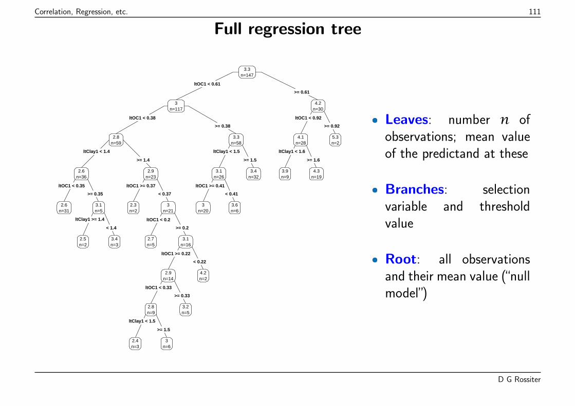
Correlation, Regression, etc. 111
Full regression tree
ltOC1 < 0.61
ltOC1 < 0.38
ltClay1 < 1.4
ltOC1 < 0.35
ltClay1 >= 1.4
ltOC1 >= 0.37
ltOC1 < 0.2
ltOC1 >= 0.22
ltOC1 < 0.33
ltClay1 < 1.5
ltClay1 < 1.5
ltOC1 >= 0.41
ltOC1 < 0.92
ltClay1 < 1.6
>= 0.61
>= 0.38
>= 1.4
>= 0.35
< 1.4
< 0.37
>= 0.2
< 0.22
>= 0.33
>= 1.5
>= 1.5
< 0.41
>= 0.92
>= 1.6
3.3n=147
3n=117
2.8n=59
2.6n=36
2.6n=31
3.1n=5
2.5n=2
3.4n=3
2.9n=23
2.3n=2
3n=21
2.7n=5
3.1n=16
2.9n=14
2.8n=9
2.4n=3
3n=6
3.2n=5
4.2n=2
3.3n=58
3.1n=26
3n=20
3.6n=6
3.4n=32
4.2n=30
4.1n=28
3.9n=9
4.3n=19
5.3n=2
� Leaves: number n ofobservations; mean valueof the predictand at these
� Branches: selectionvariable and thresholdvalue
� Root: all observationsand their mean value (“nullmodel”)
D G Rossiter
Correlation, Regression, etc. 112
Assessing over-fitting
A full tree over-fits: it fits noise specific to this dataset, i.e., this sample, rather thanstructure, common to all datasets that could be collected from the underlyingpopulation.
Assess this with x-fold cross-validation, to find the optimum tree size, we then prunethe tree to this size. Algorithm:
1. Randomly split the observations into x groups (rpart.control default is 10)..
2. For each complexity parameter (roughly, the maximum number of splits):
(a) For each group:i. Remove from the datasetii. Re-fit the tree without the removed observationsiii. Use the tree to predict at the removed observations, using their predictor valuesiv. Compute the squared error
(b) Summarize errors as root-mean-squared error (RMSE).
3. Display a table and graph of complexity parameter vs. cross-validation error
D G Rossiter
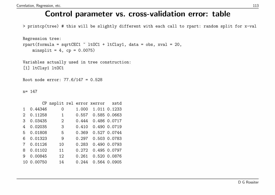
Correlation, Regression, etc. 113
Control parameter vs. cross-validation error: table
> printcp(tree) # this will be slightly different with each call to rpart: random split for x-val
Regression tree:
rpart(formula = sqrtCEC1 ~ ltOC1 + ltClay1, data = obs, xval = 20,
minsplit = 4, cp = 0.0075)
Variables actually used in tree construction:
[1] ltClay1 ltOC1
Root node error: 77.6/147 = 0.528
n= 147
CP nsplit rel error xerror xstd
1 0.44346 0 1.000 1.011 0.1233
2 0.11258 1 0.557 0.585 0.0663
3 0.03435 2 0.444 0.486 0.0717
4 0.02035 3 0.410 0.490 0.0719
5 0.01808 5 0.369 0.527 0.0744
6 0.01323 9 0.297 0.503 0.0783
7 0.01126 10 0.283 0.490 0.0793
8 0.01102 11 0.272 0.495 0.0797
9 0.00845 12 0.261 0.520 0.0876
10 0.00750 14 0.244 0.564 0.0905
D G Rossiter
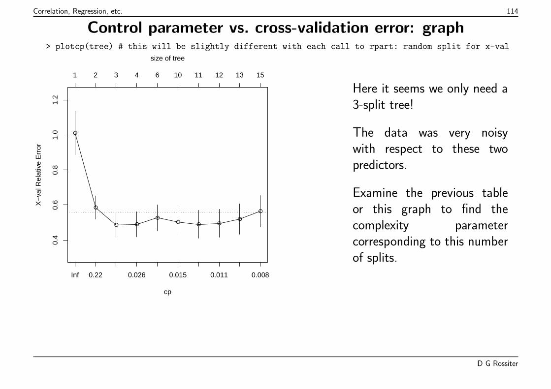
Correlation, Regression, etc. 114
Control parameter vs. cross-validation error: graph> plotcp(tree) # this will be slightly different with each call to rpart: random split for x-val
●
●
● ●
●●
● ●●
●
cp
X−
val R
elat
ive
Err
or
0.4
0.6
0.8
1.0
1.2
Inf 0.22 0.026 0.015 0.011 0.008
1 2 3 4 6 10 11 12 13 15
size of tree
Here it seems we only need a3-split tree!
The data was very noisywith respect to these twopredictors.
Examine the previous tableor this graph to find thecomplexity parametercorresponding to this numberof splits.
D G Rossiter
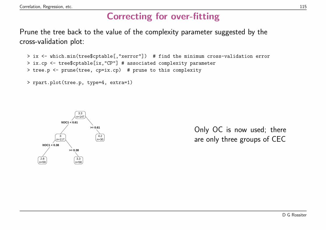
Correlation, Regression, etc. 115
Correcting for over-fitting
Prune the tree back to the value of the complexity parameter suggested by thecross-validation plot:
> ix <- which.min(tree$cptable[,"xerror"]) # find the minimum cross-validation error
> ix.cp <- tree$cptable[ix,"CP"] # associated complexity parameter
> tree.p <- prune(tree, cp=ix.cp) # prune to this complexity
> rpart.plot(tree.p, type=4, extra=1)
ltOC1 < 0.61
ltOC1 < 0.38
>= 0.61
>= 0.38
3.3n=147
3n=117
2.8n=59
3.3n=58
4.2n=30
Only OC is now used; thereare only three groups of CEC
D G Rossiter
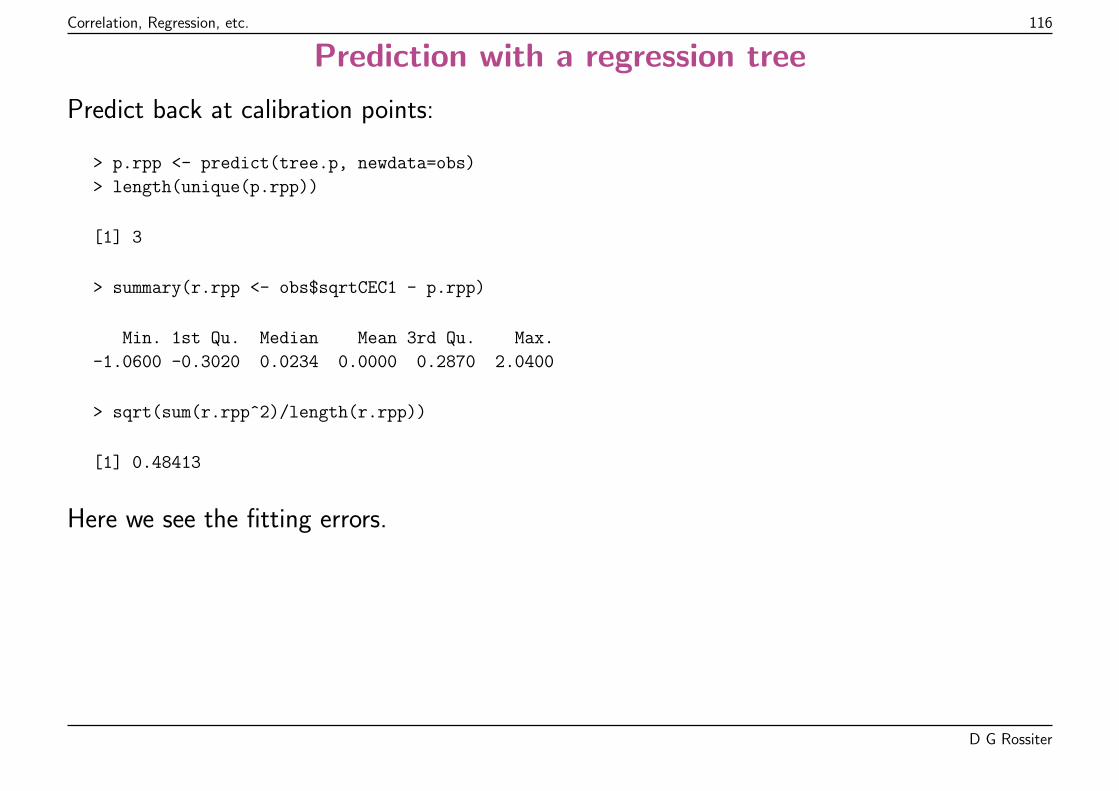
Correlation, Regression, etc. 116
Prediction with a regression tree
Predict back at calibration points:
> p.rpp <- predict(tree.p, newdata=obs)
> length(unique(p.rpp))
[1] 3
> summary(r.rpp <- obs$sqrtCEC1 - p.rpp)
Min. 1st Qu. Median Mean 3rd Qu. Max.
-1.0600 -0.3020 0.0234 0.0000 0.2870 2.0400
> sqrt(sum(r.rpp^2)/length(r.rpp))
[1] 0.48413
Here we see the fitting errors.
D G Rossiter
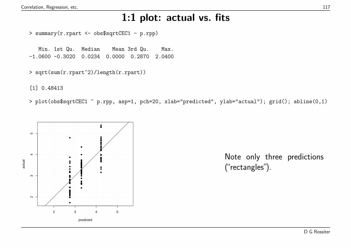
Correlation, Regression, etc. 117
1:1 plot: actual vs. fits
> summary(r.rpart <- obs$sqrtCEC1 - p.rpp)
Min. 1st Qu. Median Mean 3rd Qu. Max.
-1.0600 -0.3020 0.0234 0.0000 0.2870 2.0400
> sqrt(sum(r.rpart^2)/length(r.rpart))
[1] 0.48413
> plot(obs$sqrtCEC1 ~ p.rpp, asp=1, pch=20, xlab="predicted", ylab="actual"); grid(); abline(0,1)
●
●
●
●
●
●
●●
●
●
●
●
●
●
●
●
●
●●●
●
●
●
●
●
●
●
●
●
●
●
●
●
●
●
●
●
●
●
●
●
●
●
●
●
●
●
●
●
●
●
●
●
●
●
●
●
●
●
●
●●
●
●
●●
●
●
●
●
●
●
●
●
●●
●
●
●
●●
●
●
●
●
● ●
●
●
●
●
●
●
●
●
●
●●
●
●
●
●
●●
●
●
●
●
●
●
●
●
●
●
●
●
●
●
●
●
●
●
●
●
●
●
●●
●
●
●
●
●
●
●
●●
●
●
●
●
●
●
●
●
●
●
2 3 4 5
23
45
predicted
actu
al
Note only three predictions(“rectangles”).
D G Rossiter
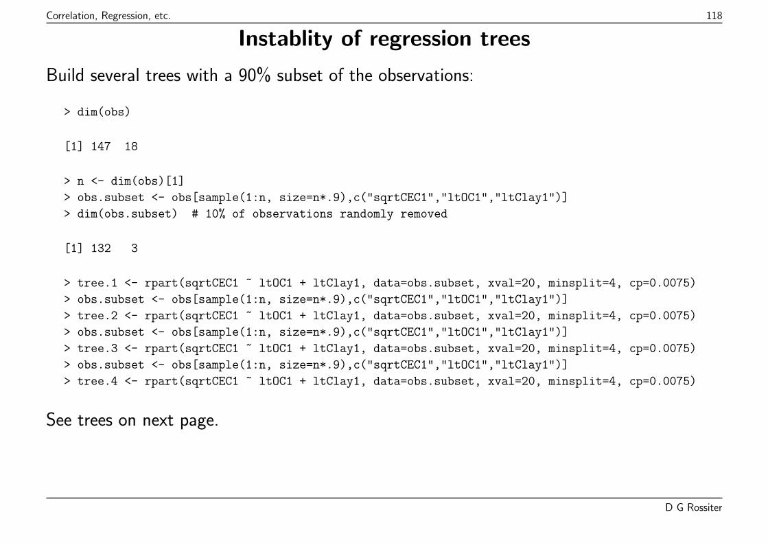
Correlation, Regression, etc. 118
Instablity of regression trees
Build several trees with a 90% subset of the observations:
> dim(obs)
[1] 147 18
> n <- dim(obs)[1]
> obs.subset <- obs[sample(1:n, size=n*.9),c("sqrtCEC1","ltOC1","ltClay1")]
> dim(obs.subset) # 10% of observations randomly removed
[1] 132 3
> tree.1 <- rpart(sqrtCEC1 ~ ltOC1 + ltClay1, data=obs.subset, xval=20, minsplit=4, cp=0.0075)
> obs.subset <- obs[sample(1:n, size=n*.9),c("sqrtCEC1","ltOC1","ltClay1")]
> tree.2 <- rpart(sqrtCEC1 ~ ltOC1 + ltClay1, data=obs.subset, xval=20, minsplit=4, cp=0.0075)
> obs.subset <- obs[sample(1:n, size=n*.9),c("sqrtCEC1","ltOC1","ltClay1")]
> tree.3 <- rpart(sqrtCEC1 ~ ltOC1 + ltClay1, data=obs.subset, xval=20, minsplit=4, cp=0.0075)
> obs.subset <- obs[sample(1:n, size=n*.9),c("sqrtCEC1","ltOC1","ltClay1")]
> tree.4 <- rpart(sqrtCEC1 ~ ltOC1 + ltClay1, data=obs.subset, xval=20, minsplit=4, cp=0.0075)
See trees on next page.
D G Rossiter
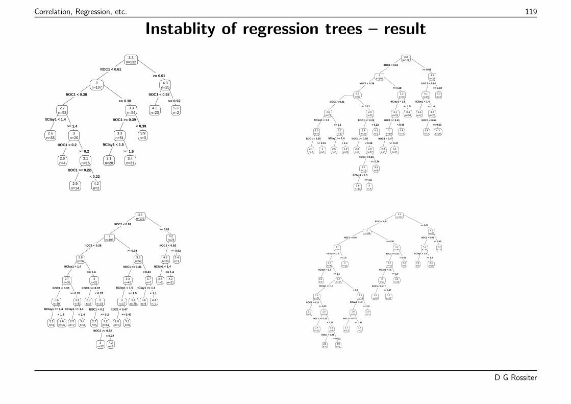
Correlation, Regression, etc. 119
Instablity of regression trees – result
ltOC1 < 0.61
ltOC1 < 0.38
ltClay1 < 1.4
ltOC1 < 0.2
ltOC1 >= 0.22
ltOC1 >= 0.39
ltClay1 < 1.5
ltOC1 < 0.92
>= 0.61
>= 0.38
>= 1.4
>= 0.2
< 0.22
< 0.39
>= 1.5
>= 0.92
3.3n=132
3n=107
2.7n=53
2.6n=33
3n=20
2.6n=4
3.1n=16
2.9n=14
4.2n=2
3.3n=54
3.3n=51
3.1n=20
3.4n=31
3.9n=3
4.3n=25
4.2n=23
5.3n=2
ltOC1 < 0.61
ltOC1 < 0.38
ltOC1 < 0.21
ltClay1 < 1.1
ltOC1 < 0.15 ltClay1 >= 1.4
ltOC1 >= 0.22
ltOC1 >= 0.38
ltOC1 < 0.34
ltClay1 < 1.5
ltClay1 < 1.5
ltOC1 >= 0.41
ltOC1 < 0.47
ltOC1 < 0.92
ltClay1 < 1.4
ltOC1 < 0.63
>= 0.61
>= 0.38
>= 0.21
>= 1.1
>= 0.15 < 1.4
< 0.22
< 0.38
>= 0.34
>= 1.5
>= 1.5
< 0.41
>= 0.47
>= 0.92
>= 1.4
>= 0.63
3.3n=132
3n=105
2.8n=52
2.6n=21
2.3n=4
2.1n=3
3n=1
2.7n=17
2.5n=8
2.9n=9
2.9n=31
2.8n=29
2.3n=2
2.8n=27
2.7n=18
2.6n=13
3n=5
3.1n=9
4.2n=2
3.3n=53
3.1n=23
3n=19
2.8n=8
3.1n=11
3.8n=4
3.4n=30
4.2n=27
4.1n=25
3.6n=2
4.2n=23
3.8n=3
4.3n=20
5.3n=2
ltOC1 < 0.61
ltOC1 < 0.38
ltClay1 < 1.4
ltOC1 < 0.35
ltClay1 >= 1.4 ltClay1 >= 1.4
ltOC1 >= 0.37
ltOC1 < 0.2
ltOC1 >= 0.22
ltOC1 >= 0.41
ltClay1 < 1.5
ltOC1 < 0.47
ltClay1 >= 1.1
ltOC1 < 0.92
ltClay1 < 1.4
>= 0.61
>= 0.38
>= 1.4
>= 0.35
< 1.4 < 1.4
< 0.37
>= 0.2
< 0.22
< 0.41
>= 1.5
>= 0.47
< 1.1
>= 0.92
>= 1.4
3.2n=132
3n=108
2.8n=56
2.7n=35
2.6n=30
2.2n=4
2.6n=26
3.1n=5
2.5n=2
3.4n=3
3n=21
2.3n=2
3n=19
2.7n=5
3.2n=14
3n=12
4.2n=2
3.3n=52
3.3n=45
3n=17
2.8n=8
3.1n=9
3.4n=28
3.7n=7
3.6n=6
4.4n=1
4.2n=24
4.2n=23
3.6n=2
4.2n=21
5.4n=1
ltOC1 < 0.61
ltOC1 < 0.38
ltClay1 < 1.5
ltClay1 < 1.1
ltClay1 >= 1.3
ltOC1 < 0.13
ltOC1 >= 0.22
ltOC1 < 0.21
ltClay1 < 1.3
ltOC1 < 0.33
ltOC1 >= 0.41
ltClay1 < 1.5
ltOC1 < 0.47
ltOC1 < 0.92
ltClay1 < 1.6
>= 0.61
>= 0.38
>= 1.5
>= 1.1
< 1.3
>= 0.13
< 0.22
>= 0.21
>= 1.3
>= 0.33
< 0.41
>= 1.5
>= 0.47
>= 0.92
>= 1.6
3.3n=132
3n=104
2.7n=54
2.7n=42
2.4n=5
2.7n=37
2.6n=21
2.1n=2
2.6n=19
2.5n=13
2.9n=6
2.5n=5
4.8n=1
2.8n=16
2.8n=15
2.7n=13
3.5n=2
3.9n=1
3n=12
3.3n=50
3.2n=42
3n=22
2.8n=10
3.2n=12
3.5n=20
3.6n=8
4.2n=28
4.1n=26
3.8n=8
4.3n=18
5.3n=2
D G Rossiter
Correlation, Regression, etc. 120
Random forests
Problems with regression trees:
1. A small change in the sample set (e.g., a missing or erroneous observation) can make alarge change in the tree;
2. Sub-optimal splits propagate down the tree (there is no way to backtrack);
3. Correlated predictors are only used one way;
4. Discontinuous predictions (“rectangles”);
5. Different cross-validation splits suggest different complexity parameters for smoothing.
Solution: why one tree when you can have a forest?
D G Rossiter
Correlation, Regression, etc. 121
Procedure
1. Build a large number of regression trees, independently, using different sets ofobservations.
2. These are built by sampling with replacement from the actual observations.
� This is sometimes called bagging: some observations are“in the bag” (used tobuild the tree) and others“out of bag” (used to assess prediction error, see below).
� Note! this assumes that the sample fairly represents the population!
3. At each split, randomly select a predictor.
4. Save all these trees; when predicting, use all of them and average their predictions.
5. For each tree we can use observations that were not used to construct it for truevalidation, called out-of-bag validation. This gives a good idea of the true predictionerror.
D G Rossiter
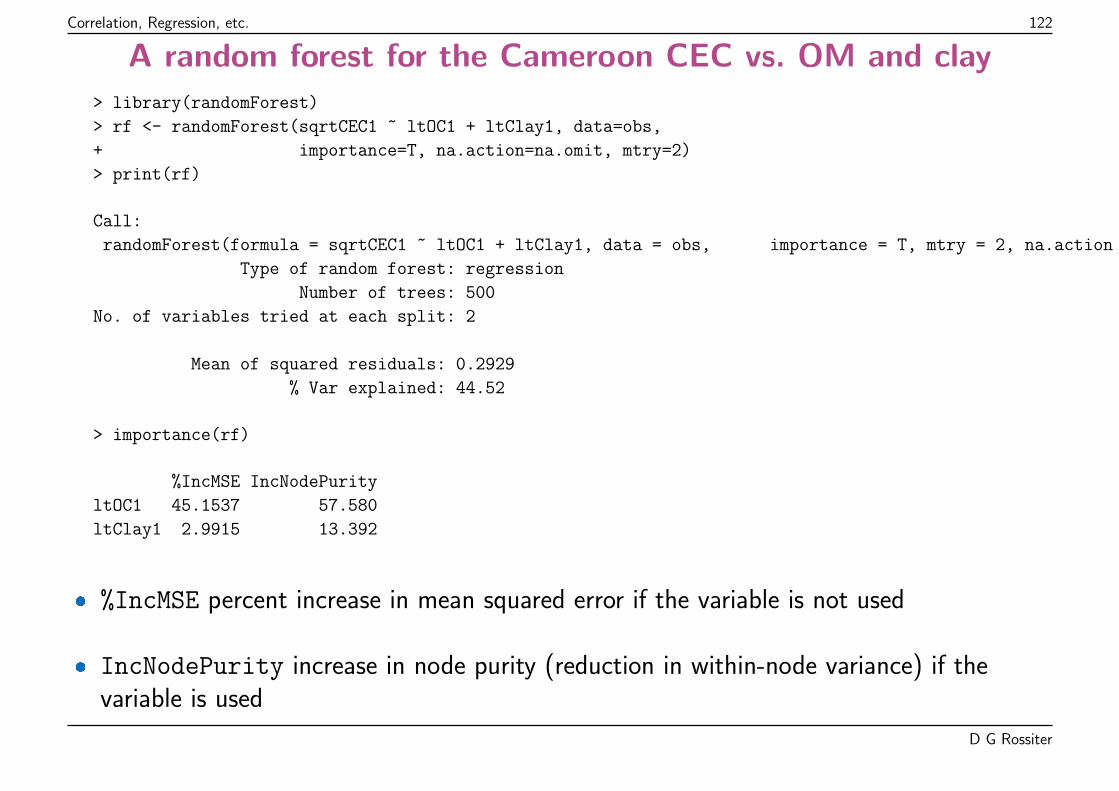
Correlation, Regression, etc. 122
A random forest for the Cameroon CEC vs. OM and clay> library(randomForest)
> rf <- randomForest(sqrtCEC1 ~ ltOC1 + ltClay1, data=obs,
+ importance=T, na.action=na.omit, mtry=2)
> print(rf)
Call:
randomForest(formula = sqrtCEC1 ~ ltOC1 + ltClay1, data = obs, importance = T, mtry = 2, na.action = na.omit)
Type of random forest: regression
Number of trees: 500
No. of variables tried at each split: 2
Mean of squared residuals: 0.2929
% Var explained: 44.52
> importance(rf)
%IncMSE IncNodePurity
ltOC1 45.1537 57.580
ltClay1 2.9915 13.392
� %IncMSE percent increase in mean squared error if the variable is not used
� IncNodePurity increase in node purity (reduction in within-node variance) if thevariable is used
D G Rossiter
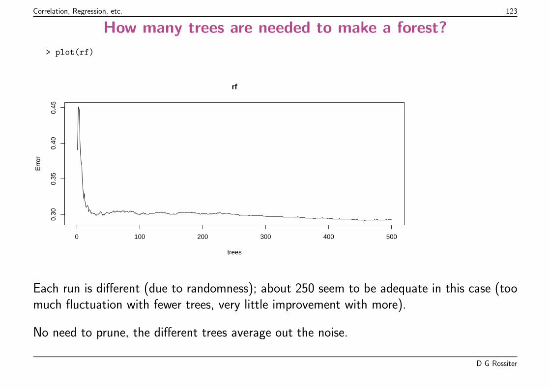
Correlation, Regression, etc. 123
How many trees are needed to make a forest?
> plot(rf)
0 100 200 300 400 500
0.30
0.35
0.40
0.45
rf
trees
Err
or
Each run is different (due to randomness); about 250 seem to be adequate in this case (toomuch fluctuation with fewer trees, very little improvement with more).
No need to prune, the different trees average out the noise.
D G Rossiter
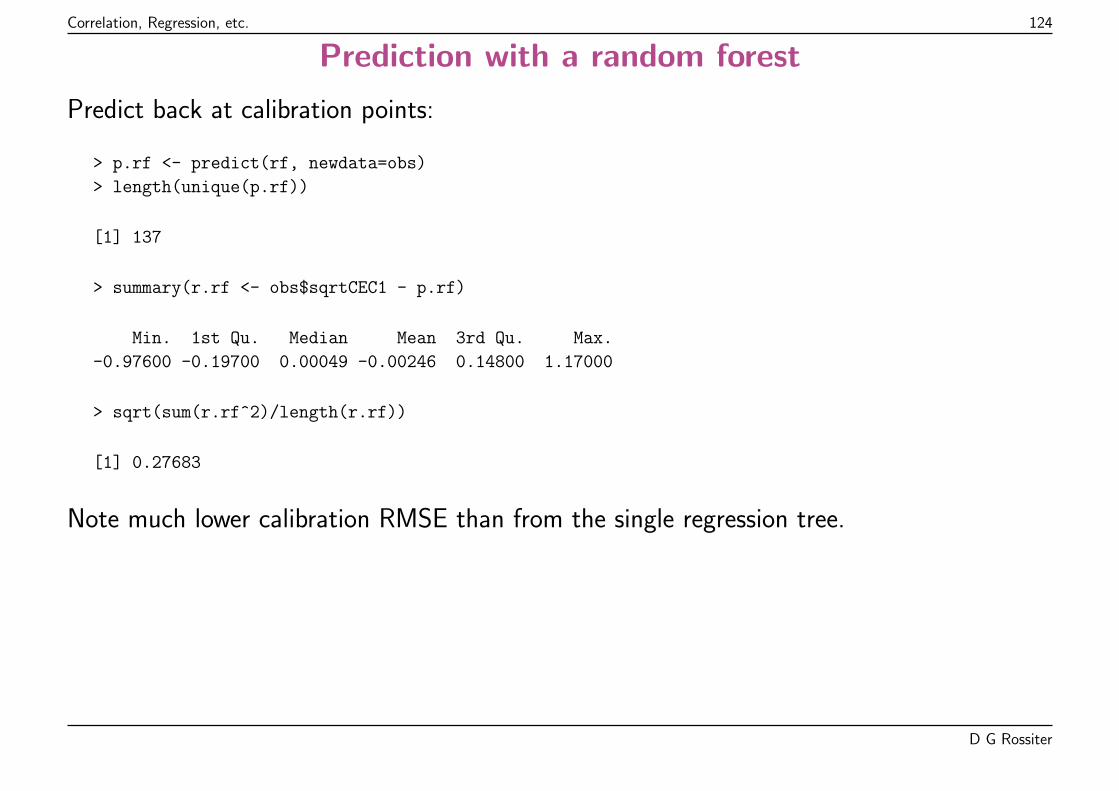
Correlation, Regression, etc. 124
Prediction with a random forest
Predict back at calibration points:
> p.rf <- predict(rf, newdata=obs)
> length(unique(p.rf))
[1] 137
> summary(r.rf <- obs$sqrtCEC1 - p.rf)
Min. 1st Qu. Median Mean 3rd Qu. Max.
-0.97600 -0.19700 0.00049 -0.00246 0.14800 1.17000
> sqrt(sum(r.rf^2)/length(r.rf))
[1] 0.27683
Note much lower calibration RMSE than from the single regression tree.
D G Rossiter
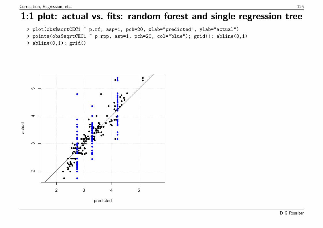
Correlation, Regression, etc. 125
1:1 plot: actual vs. fits: random forest and single regression tree> plot(obs$sqrtCEC1 ~ p.rf, asp=1, pch=20, xlab="predicted", ylab="actual")
> points(obs$sqrtCEC1 ~ p.rpp, asp=1, pch=20, col="blue"); grid(); abline(0,1)
> abline(0,1); grid()
●
●
●
●
●
●
●●
●
●
●
●
●
●
●
●
●
●●●
●
●
●
●
●
●
●
●
●
●
●
●
●
●
●
●
●
●
●
●
●
●
●
●
●
●
●
●
●
●
●
●
●
●
●
●
●
●
●
●
●●
●
●
●●
●
●
●
●
●
●
●
●
●●
●
●
●
● ●
●
●
●
●
●●
●
●
●
●
●
●
●
●
●
●●
●
●
●
●
●●
●
●
●
●
●
●
●
●
●
●
●
●
●
●
●
●
●
●
●
●
●
●
●●
●
●
●
●
●
●
●
● ●
●
●
●
●
●
●
●
●
●
●
2 3 4 5
23
45
predicted
actu
al ●
●
●
●
●
●
●●
●
●
●
●
●
●
●
●
●
●●●
●
●
●
●
●
●
●
●
●
●
●
●
●
●
●
●
●
●
●
●
●
●
●
●
●
●
●
●
●
●
●
●
●
●
●
●
●
●
●
●
●●
●
●
●●
●
●
●
●
●
●
●
●
●●
●
●
●
●●
●
●
●
●
● ●
●
●
●
●
●
●
●
●
●
●●
●
●
●
●
●●
●
●
●
●
●
●
●
●
●
●
●
●
●
●
●
●
●
●
●
●
●
●
●●
●
●
●
●
●
●
●
●●
●
●
●
●
●
●
●
●
●
●
D G Rossiter
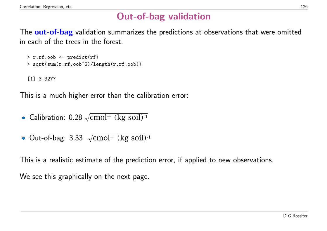
Correlation, Regression, etc. 126
Out-of-bag validation
The out-of-bag validation summarizes the predictions at observations that were omittedin each of the trees in the forest.
> r.rf.oob <- predict(rf)
> sqrt(sum(r.rf.oob^2)/length(r.rf.oob))
[1] 3.3277
This is a much higher error than the calibration error:
� Calibration: 0.28√
cmol+ (kg soil)-1
� Out-of-bag: 3.33√
cmol+ (kg soil)-1
This is a realistic estimate of the prediction error, if applied to new observations.
We see this graphically on the next page.
D G Rossiter
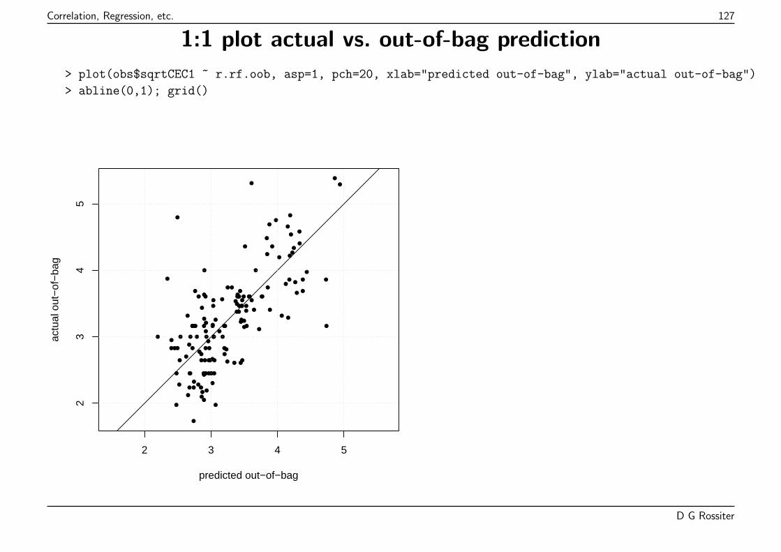
Correlation, Regression, etc. 127
1:1 plot actual vs. out-of-bag prediction
> plot(obs$sqrtCEC1 ~ r.rf.oob, asp=1, pch=20, xlab="predicted out-of-bag", ylab="actual out-of-bag")
> abline(0,1); grid()
●
●
●
●
●
●
●●
●
●
●
●
●
●
●
●
●
●●●
●
●
●
●
●
●
●
●
●
●
●
●
●
●
●
●
●
●
●
●
●
●
●
●
●
●
●
●
●
●
●
●
●
●
●
●
●
●
●
●
●●
●
●
●●
●
●
●
●
●
●
●
●
● ●
●
●
●
● ●
●
●
●
●
●●
●
●
●
●
●
●
●
●
●
●●
●
●
●
●
●●
●
●
●
●
●
●
●
●
●
●
●
●
●
●
●
●
●
●
●
●
●
●
●●
●
●
●
●
●
●
●
● ●
●
●
●
●
●
●
●
●
●
●
2 3 4 5
23
45
predicted out−of−bag
actu
al o
ut−
of−
bag
D G Rossiter
Correlation, Regression, etc. 128
Topic: Factor Analysis
Here we consider the inter-relations between a set of variables
� Often the set of predictors which might be used in a multiple linear regression.
This is an analysis of the structure of the multivariate feature space covered by a setof variables.
Uses:
1. Discover relations between variables, and possible groupings
2. Diagnose multi-collinearity;
3. Identify representative variables, e.g., for a minimum data set to be used in regression;
4. Define synthetic variables to be used directly in regression.
D G Rossiter
Correlation, Regression, etc. 129
Principal Components Analysis (PCA)
The simplest form of factor analysis; it is a multivariate data reduction technique.
� The vector space made up of the original variables is projected onto another space;
� The new space has the same dimensionality as the original1, i.e., there are as manyvariables in the new space as in the old;
� In this space the new synthetic variables, also called principal components areorthogonal to each other, i.e. completely uncorrelated;
� The synthetic variables are arranged in decreasing order of variance explained.
These synthetic variables can often be interpreted by the analyst, that is, they representsome composite attribute of the objects of study.
1unless the original was rank-deficientD G Rossiter
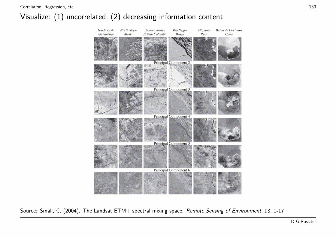
Correlation, Regression, etc. 130
Visualize: (1) uncorrelated; (2) decreasing information content
Source: Small, C. (2004). The Landsat ETM+ spectral mixing space. Remote Sensing of Environment, 93, 1-17
D G Rossiter
Correlation, Regression, etc. 131
Standardized or not
Two forms:
Standardized each variable has its mean subtracted (so x.j = 0) and is divided by itssample standard deviation (so σ(x.j) = 1);
� All variables are equally important, no matter their absolute values or spreads;� This is usually what we want.
Unstandardized use the original variables, in their original scales of measurement;generally the means are also subtracted to centre the variables
� Variables with larger absolute values and wider spreads are more important, sincethey contribute more to the original variance
D G Rossiter
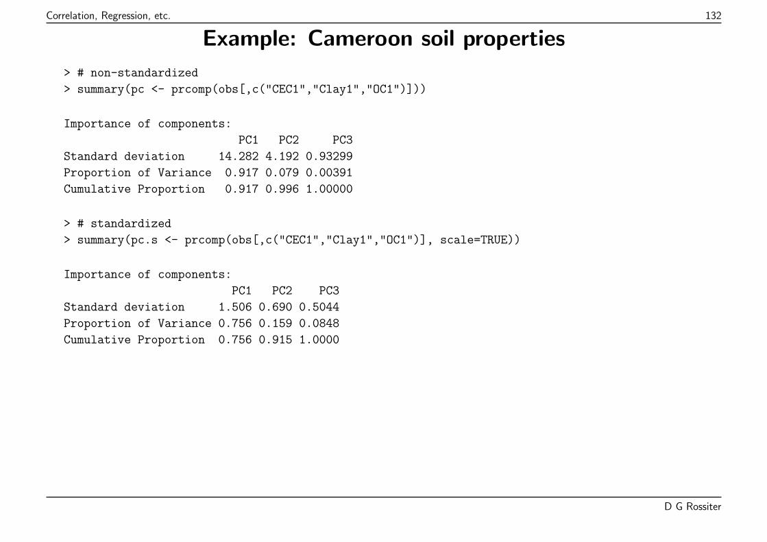
Correlation, Regression, etc. 132
Example: Cameroon soil properties
> # non-standardized
> summary(pc <- prcomp(obs[,c("CEC1","Clay1","OC1")]))
Importance of components:
PC1 PC2 PC3
Standard deviation 14.282 4.192 0.93299
Proportion of Variance 0.917 0.079 0.00391
Cumulative Proportion 0.917 0.996 1.00000
> # standardized
> summary(pc.s <- prcomp(obs[,c("CEC1","Clay1","OC1")], scale=TRUE))
Importance of components:
PC1 PC2 PC3
Standard deviation 1.506 0.690 0.5044
Proportion of Variance 0.756 0.159 0.0848
Cumulative Proportion 0.756 0.915 1.0000
D G Rossiter
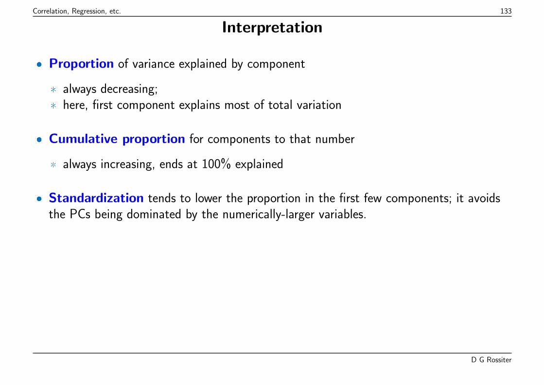
Correlation, Regression, etc. 133
Interpretation
� Proportion of variance explained by component
* always decreasing;* here, first component explains most of total variation
� Cumulative proportion for components to that number
* always increasing, ends at 100% explained
� Standardization tends to lower the proportion in the first few components; it avoidsthe PCs being dominated by the numerically-larger variables.
D G Rossiter
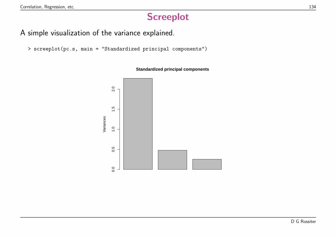
Correlation, Regression, etc. 134
Screeplot
A simple visualization of the variance explained.
> screeplot(pc.s, main = "Standardized principal components")
Standardized principal components
Var
ianc
es
0.0
0.5
1.0
1.5
2.0
D G Rossiter
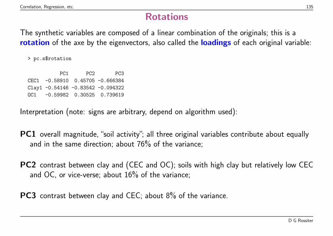
Correlation, Regression, etc. 135
Rotations
The synthetic variables are composed of a linear combination of the originals; this is arotation of the axe by the eigenvectors, also called the loadings of each original variable:
> pc.s$rotation
PC1 PC2 PC3
CEC1 -0.58910 0.45705 -0.666384
Clay1 -0.54146 -0.83542 -0.094322
OC1 -0.59982 0.30525 0.739619
Interpretation (note: signs are arbitrary, depend on algorithm used):
PC1 overall magnitude, “soil activity”; all three original variables contribute about equallyand in the same direction; about 76% of the variance;
PC2 contrast between clay and (CEC and OC); soils with high clay but relatively low CECand OC, or vice-verse; about 16% of the variance;
PC3 contrast between clay and CEC; about 8% of the variance.
D G Rossiter
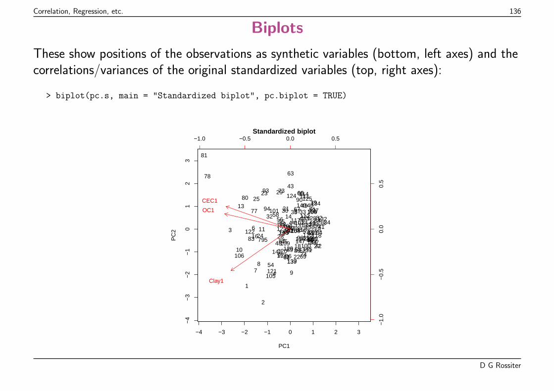
Correlation, Regression, etc. 136
Biplots
These show positions of the observations as synthetic variables (bottom, left axes) and thecorrelations/variances of the original standardized variables (top, right axes):
> biplot(pc.s, main = "Standardized biplot", pc.biplot = TRUE)
−4 −3 −2 −1 0 1 2 3
−4
−3
−2
−1
01
23
Standardized biplot
PC1
PC
2
1
2
3
4
5
6
78
9
10
11 12
13
14
15
16
17
18
19
20
21
22
23
24
25
26
27
28
29
30
31
3233
34
35
36
37
38
3940
41
42
43
44
45
4647
48
49
5051
5253
54
55
56
57
58
5960
6162
63
64
6566
67
68
69
707172
73
74
7576
77
78
79
80
81
82
83
84
8586
87
88
89
90
91
92
93
94
95
96
97
98
99
100
101
102103
104
105
106
107
108
109110
111
112
113
114
115116
117
118119
120
121
122123
124 125
126127
128
129
130
131132
133
134135
136
137
138
139
140
141
142
143
144145
146
147
−1.0 −0.5 0.0 0.5
−1.
0−
0.5
0.0
0.5
CEC1
Clay1
OC1
D G Rossiter
Correlation, Regression, etc. 137
Interpretation of biplots
� Length of vector is variance explained in this plane;
� Angle between vectors is degree of correlation (closer = more correlated);
� Individual observations are plotted with their PC scores (values in the PC space);
� Points close in this space have similar properties with respect to these two PCs.
D G Rossiter
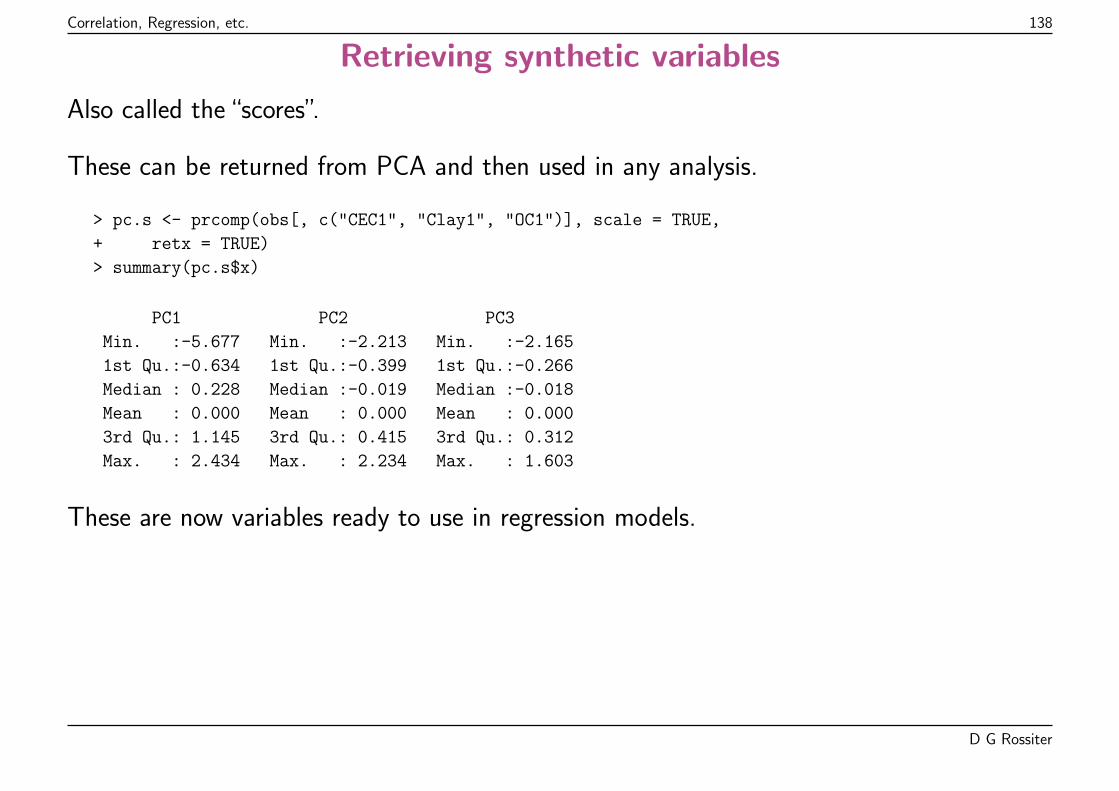
Correlation, Regression, etc. 138
Retrieving synthetic variables
Also called the “scores”.
These can be returned from PCA and then used in any analysis.
> pc.s <- prcomp(obs[, c("CEC1", "Clay1", "OC1")], scale = TRUE,
+ retx = TRUE)
> summary(pc.s$x)
PC1 PC2 PC3
Min. :-5.677 Min. :-2.213 Min. :-2.165
1st Qu.:-0.634 1st Qu.:-0.399 1st Qu.:-0.266
Median : 0.228 Median :-0.019 Median :-0.018
Mean : 0.000 Mean : 0.000 Mean : 0.000
3rd Qu.: 1.145 3rd Qu.: 0.415 3rd Qu.: 0.312
Max. : 2.434 Max. : 2.234 Max. : 1.603
These are now variables ready to use in regression models.
D G Rossiter
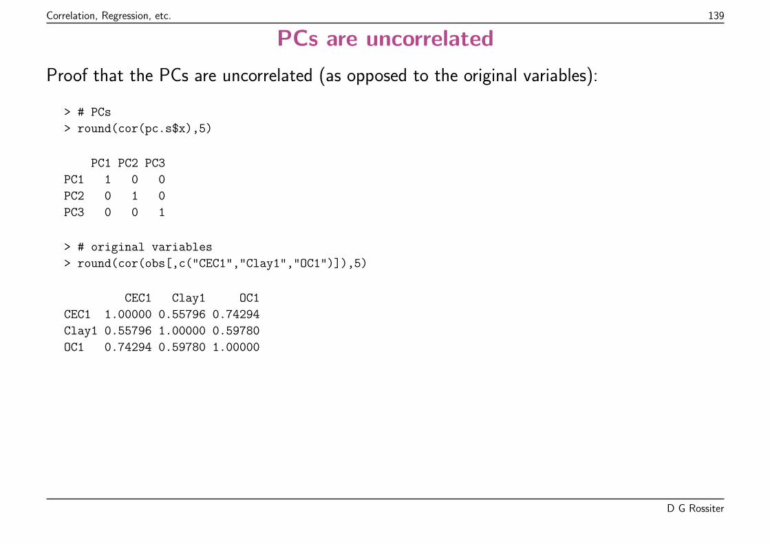
Correlation, Regression, etc. 139
PCs are uncorrelated
Proof that the PCs are uncorrelated (as opposed to the original variables):
> # PCs
> round(cor(pc.s$x),5)
PC1 PC2 PC3
PC1 1 0 0
PC2 0 1 0
PC3 0 0 1
> # original variables
> round(cor(obs[,c("CEC1","Clay1","OC1")]),5)
CEC1 Clay1 OC1
CEC1 1.00000 0.55796 0.74294
Clay1 0.55796 1.00000 0.59780
OC1 0.74294 0.59780 1.00000
D G Rossiter
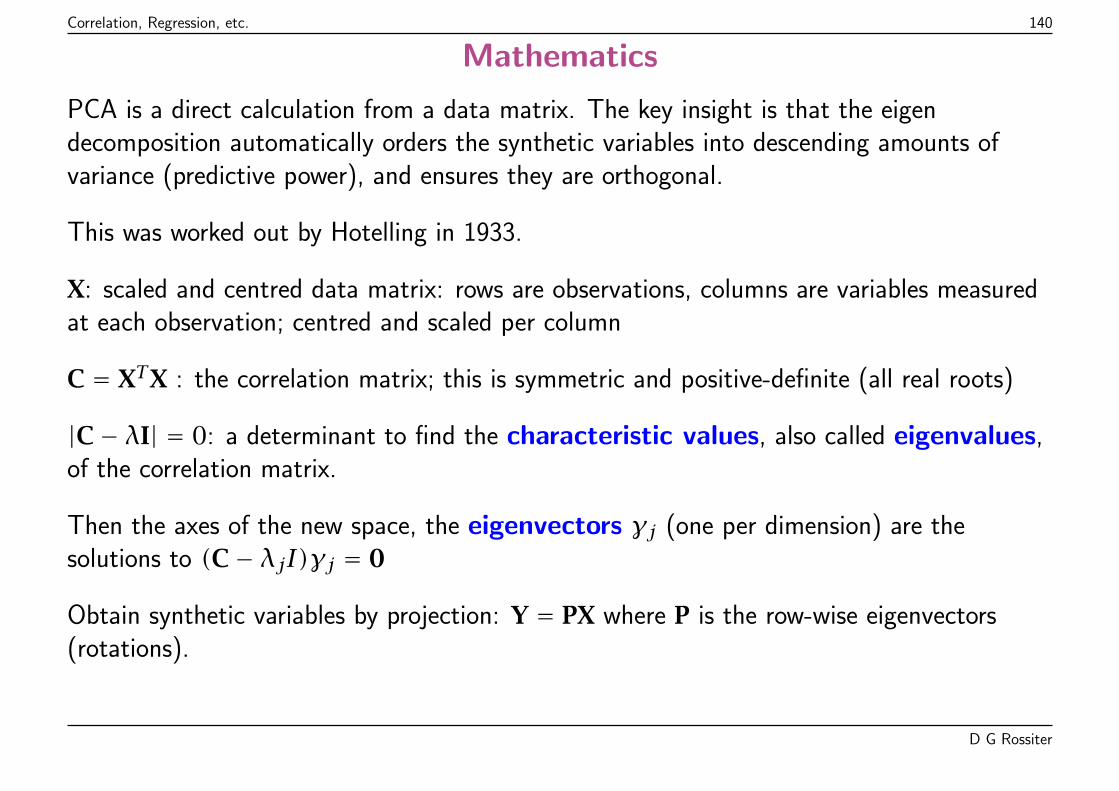
Correlation, Regression, etc. 140
Mathematics
PCA is a direct calculation from a data matrix. The key insight is that the eigendecomposition automatically orders the synthetic variables into descending amounts ofvariance (predictive power), and ensures they are orthogonal.
This was worked out by Hotelling in 1933.
X: scaled and centred data matrix: rows are observations, columns are variables measuredat each observation; centred and scaled per column
C = XTX : the correlation matrix; this is symmetric and positive-definite (all real roots)
|C− λI| = 0: a determinant to find the characteristic values, also called eigenvalues,of the correlation matrix.
Then the axes of the new space, the eigenvectors γj (one per dimension) are thesolutions to (C− λjI)γj = 0
Obtain synthetic variables by projection: Y = PX where P is the row-wise eigenvectors(rotations).
D G Rossiter
Correlation, Regression, etc. 141
Details
In practice the system is solved by the Singular Value Decomposition (SVD) of the datamatrix, for numerical stability.
This is equivalent but more stable than directly extracting the eigenvectors of thecorrelation matrix.
Accessible explanations:
� Davis, J. C. (2002). Statistics and data analysis in geology. New York: John Wiley &Sons.
� Legendre, P., & Legendre, L. (1998). Numerical ecology. Oxford: Elsevier Science.
D G Rossiter
Correlation, Regression, etc. 142
Topic: Linear model for categorical predictors
Predictors may be categorical:
� Nominal: unordered categories
� Ordinal: categories with a natural order but not on an interval scale
These can also be modelled with the linear model y = BX + ε.
D G Rossiter
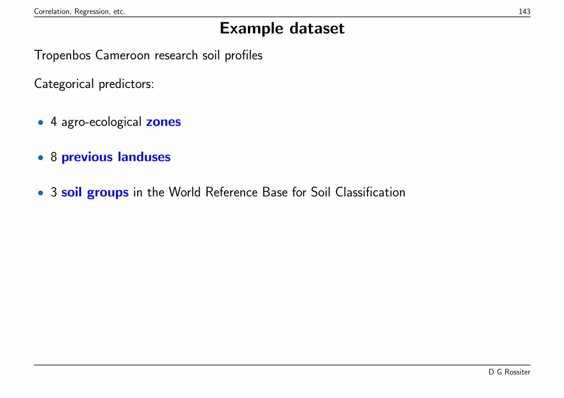
Correlation, Regression, etc. 143
Example dataset
Tropenbos Cameroon research soil profiles
Categorical predictors:
� 4 agro-ecological zones
� 8 previous landuses
� 3 soil groups in the World Reference Base for Soil Classification
D G Rossiter
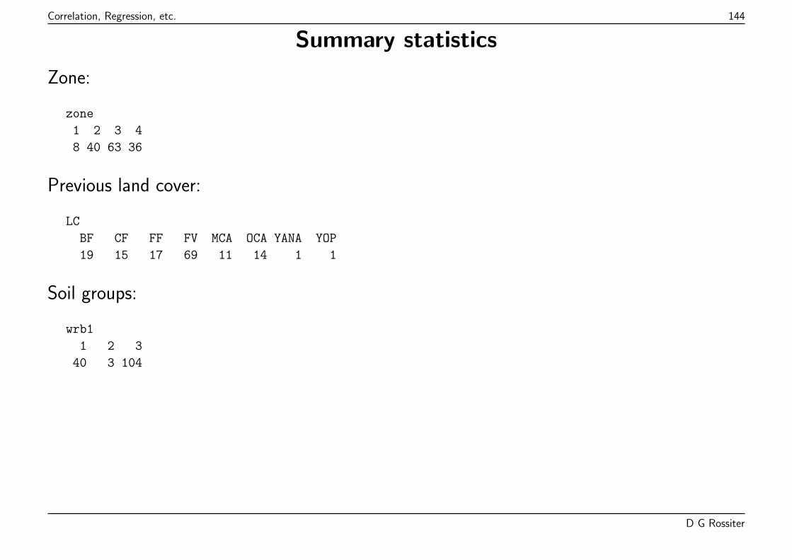
Correlation, Regression, etc. 144
Summary statistics
Zone:
zone
1 2 3 4
8 40 63 36
Previous land cover:
LC
BF CF FF FV MCA OCA YANA YOP
19 15 17 69 11 14 1 1
Soil groups:
wrb1
1 2 3
40 3 104
D G Rossiter
Correlation, Regression, etc. 145
Model from a single categorical predictor
Research question: do the different zones (represented by villages) have different soilproperties?
Example: topsoil clay content (log-transformed)
D G Rossiter
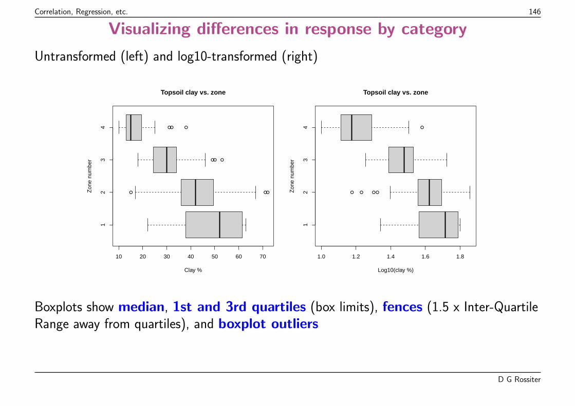
Correlation, Regression, etc. 146
Visualizing differences in response by category
Untransformed (left) and log10-transformed (right)
●●●
● ●●
●●●
12
34
10 20 30 40 50 60 70
Topsoil clay vs. zone
Clay %
Zon
e nu
mbe
r
●● ● ●
●
12
34
1.0 1.2 1.4 1.6 1.8
Topsoil clay vs. zone
Log10(clay %)
Zon
e nu
mbe
r
Boxplots show median, 1st and 3rd quartiles (box limits), fences (1.5 x Inter-QuartileRange away from quartiles), and boxplot outliers
D G Rossiter
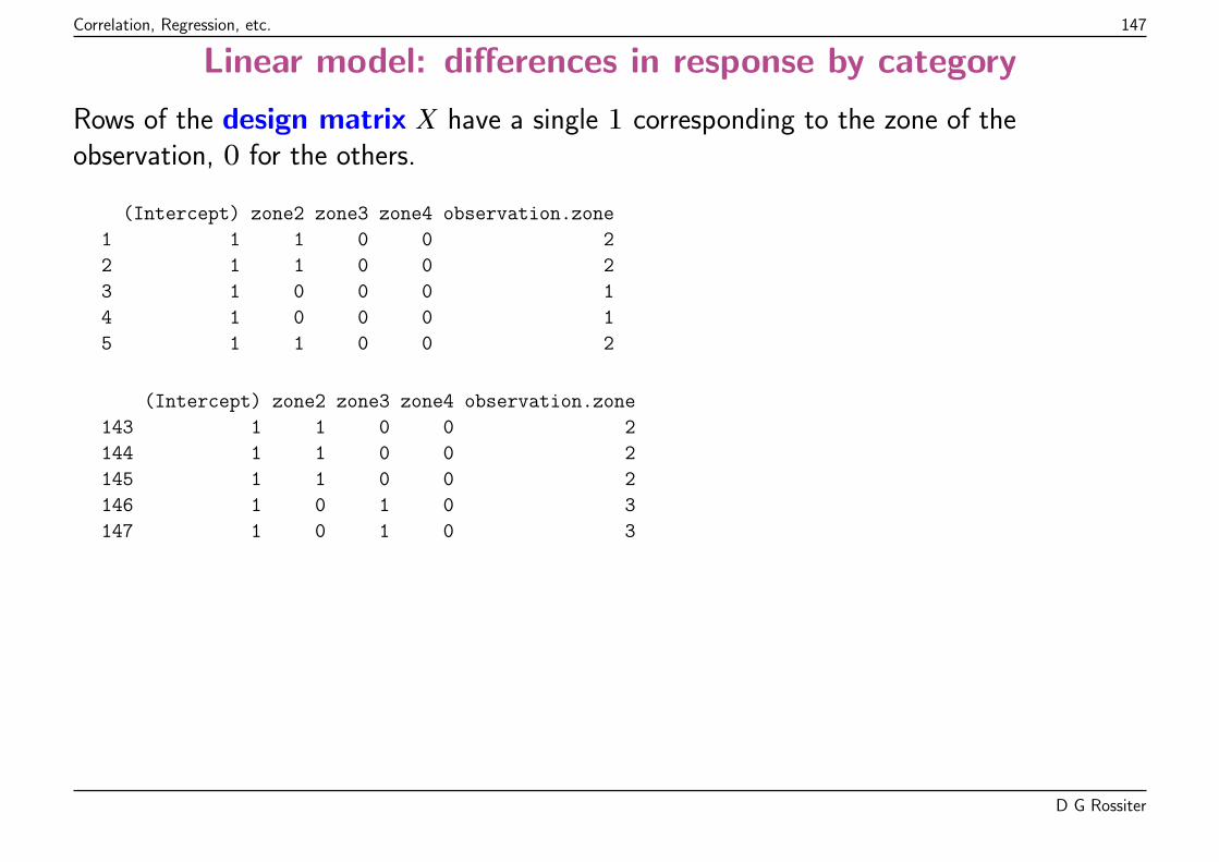
Correlation, Regression, etc. 147
Linear model: differences in response by category
Rows of the design matrix X have a single 1 corresponding to the zone of theobservation, 0 for the others.
(Intercept) zone2 zone3 zone4 observation.zone
1 1 1 0 0 2
2 1 1 0 0 2
3 1 0 0 0 1
4 1 0 0 0 1
5 1 1 0 0 2
(Intercept) zone2 zone3 zone4 observation.zone
143 1 1 0 0 2
144 1 1 0 0 2
145 1 1 0 0 2
146 1 0 1 0 3
147 1 0 1 0 3
D G Rossiter
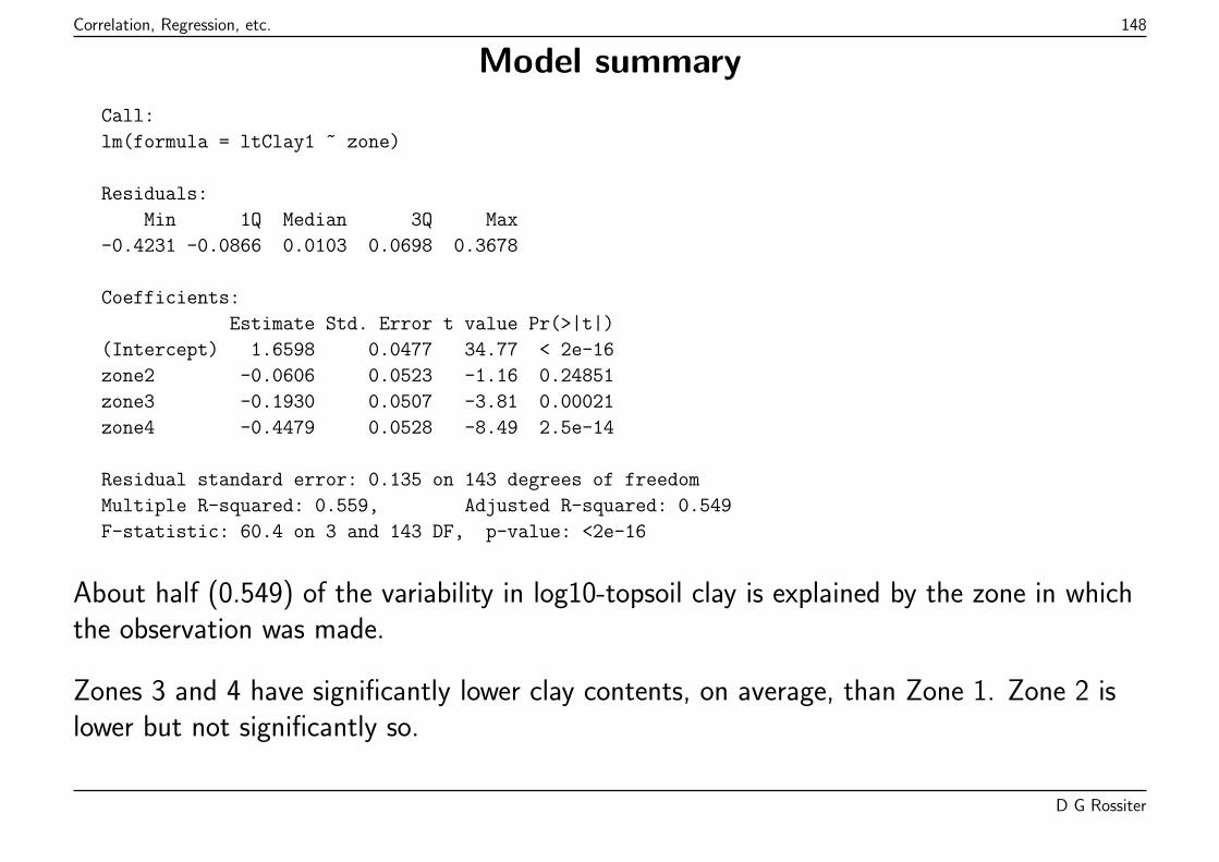
Correlation, Regression, etc. 148
Model summary
Call:
lm(formula = ltClay1 ~ zone)
Residuals:
Min 1Q Median 3Q Max
-0.4231 -0.0866 0.0103 0.0698 0.3678
Coefficients:
Estimate Std. Error t value Pr(>|t|)
(Intercept) 1.6598 0.0477 34.77 < 2e-16
zone2 -0.0606 0.0523 -1.16 0.24851
zone3 -0.1930 0.0507 -3.81 0.00021
zone4 -0.4479 0.0528 -8.49 2.5e-14
Residual standard error: 0.135 on 143 degrees of freedom
Multiple R-squared: 0.559, Adjusted R-squared: 0.549
F-statistic: 60.4 on 3 and 143 DF, p-value: <2e-16
About half (0.549) of the variability in log10-topsoil clay is explained by the zone in whichthe observation was made.
Zones 3 and 4 have significantly lower clay contents, on average, than Zone 1. Zone 2 islower but not significantly so.
D G Rossiter
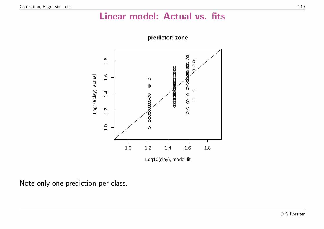
Correlation, Regression, etc. 149
Linear model: Actual vs. fits
●●
●
●
●●
●●
●
●
●
●
●
●
●
●
●
●
●●
●
●
●
●
●
●
●
●
●
●●
●
●
●
●
●
●
●
●
●
●
●
●
●
●
●
●
●
●
●●
●●
●
●
●
●
●●
●
●●
●
●
●●
●
●
●●●
●
●
●●●
●
●●
●●
●
●
●
●
●●
●
●
●
●
●●
●
●
●
●
●●●
●
●
●
●
●
●
●
●
●
●
●
●
●
●
●●●
●●
●
●●
●
●
●
●
●
●
●
●●
●
●
●
●
●
●
●
●
●
●
●
●
●
●
●
●
1.0 1.2 1.4 1.6 1.8
1.0
1.2
1.4
1.6
1.8
predictor: zone
Log10(clay), model fit
Log1
0(cl
ay),
act
ual
Note only one prediction per class.
D G Rossiter
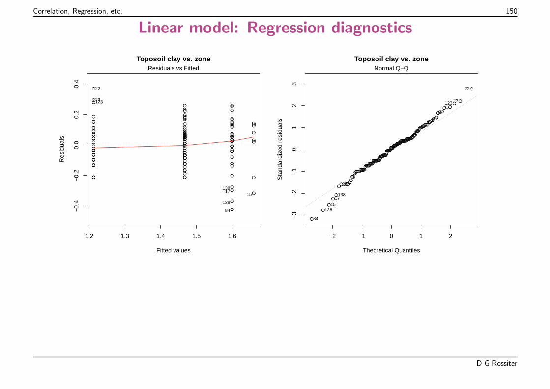
Correlation, Regression, etc. 150
Linear model: Regression diagnostics
1.2 1.3 1.4 1.5 1.6
−0.
4−
0.2
0.0
0.2
0.4
Toposoil clay vs. zone
Fitted values
Res
idua
ls
●●
●
●●
●
●
●
●
●
●
●
●
●
●
●
●
●
●●
●
●
●
●
●
●
●
●
●
●
●
●
●
●
●
●
●
●
●
●
●
●
●
● ●
●
●
●
●
●●
●●
●
●
●
●
●●
●
●●
●
●
●●
●
●
●●●
●
●
●●●
●
●●
●●
●
●
●
●
●
●
●
●●
●
●
●
●
●
●
●
●●●
●
●
●
●
●
●
●
● ●
●●
●●
●
●●●
●
●
●
●●
●
●
●
●
●
●
●
●●
●
●
●
●
●
●
●
●
●
● ●
●
●
●
●
●
Residuals vs Fitted
84
128
22
1517
23123
138
●●
●
●●
●
●●
●
●
●
●
●
●
●
●
●
●
●●
●
●
●
●
●
●
●
●
●
●
●
●
●
●
●
●
●
●
●
●
●
●
●
●●
●
●
●
●
●●
●●
●
●
●
●
●●
●
●●
●
●
●●
●
●
●●
●
●
●
●●
●
●
●●
●●
●
●
●
●
●
●
●
●●
●
●
●
●
●
●
●
●●●
●
●
●
●
●
●
●
●●
●
●
●●
●
●●●
●
●
●
●●
●
●
●
●
●
●
●
●●
●
●
●
●
●
●
●
●
●
●●
●
●
●
●
●
−2 −1 0 1 2
−3
−2
−1
01
23
Toposoil clay vs. zone
Theoretical Quantiles
Sta
ndar
dize
d re
sidu
als
Normal Q−Q
84
128
22
1517
23123
138
D G Rossiter
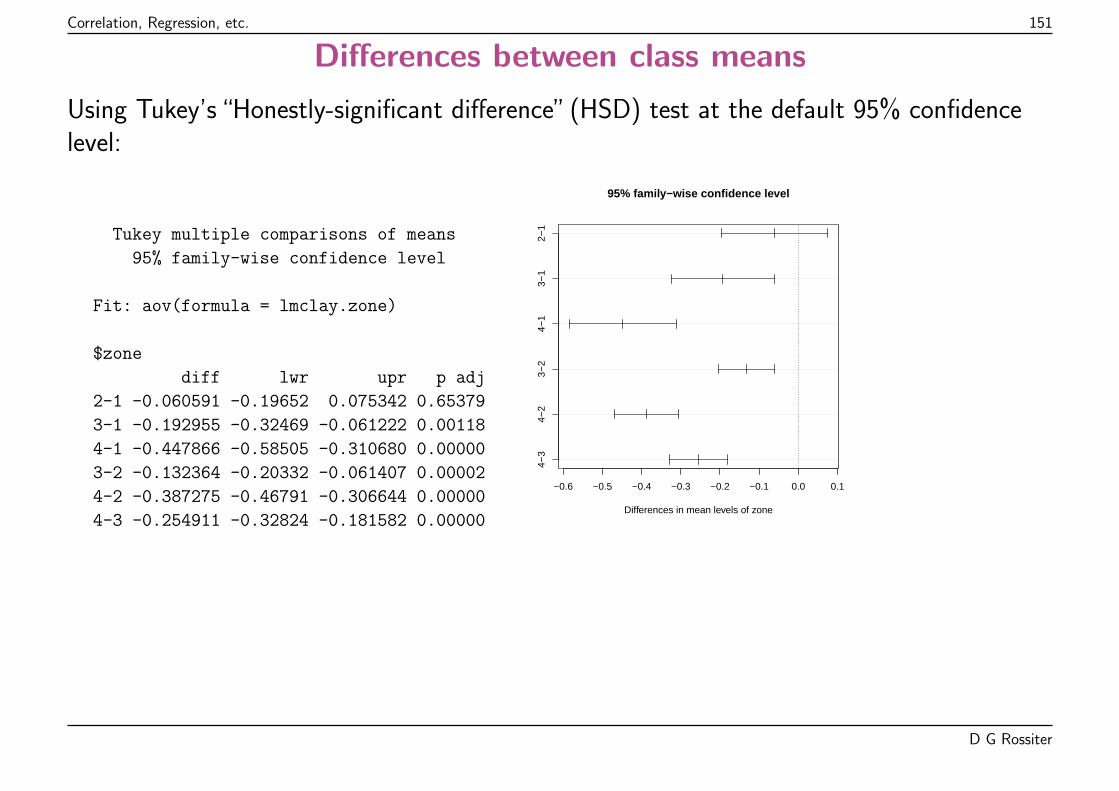
Correlation, Regression, etc. 151
Differences between class means
Using Tukey’s “Honestly-significant difference” (HSD) test at the default 95% confidencelevel:
Tukey multiple comparisons of means
95% family-wise confidence level
Fit: aov(formula = lmclay.zone)
$zone
diff lwr upr p adj
2-1 -0.060591 -0.19652 0.075342 0.65379
3-1 -0.192955 -0.32469 -0.061222 0.00118
4-1 -0.447866 -0.58505 -0.310680 0.00000
3-2 -0.132364 -0.20332 -0.061407 0.00002
4-2 -0.387275 -0.46791 -0.306644 0.00000
4-3 -0.254911 -0.32824 -0.181582 0.00000
−0.6 −0.5 −0.4 −0.3 −0.2 −0.1 0.0 0.1
4−3
4−2
3−2
4−1
3−1
2−1
95% family−wise confidence level
Differences in mean levels of zone
D G Rossiter
Correlation, Regression, etc. 152
Topic: Mixed models
It is possible to mix both continuous and categorical predictors in one model.
This is a form of multiple linear regression
The linear model form y = BX+ ε is applicable.
D G Rossiter
Correlation, Regression, etc. 153
A simple mixed model
Objective: to predict the subsoil clay content (30–50 cm depth) from the topsoil claycontent (0–10 cm depth) and/or zone.
Purpose: avoid expensive / laborious augering to 50 cm and extra lab. work
D G Rossiter
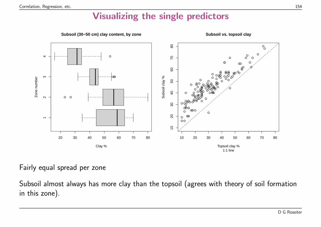
Correlation, Regression, etc. 154
Visualizing the single predictors
●●
●●●●
●
12
34
20 30 40 50 60 70 80
Subsoil (30−50 cm) clay content, by zone
Clay %
Zon
e nu
mbe
r
●●
●
●
●
●
●●
●
●
●
●●
●●
●
●
●
●
●
●
●
●
●
●●
●
●
●
●● ●
●
●
●
●●
●
●
●
●
●
●
●
●
●
●
●
●
●
●
●
●
●
● ●●
●●●
●●
●
●
●●
●●
●
●
●
●
●
●
●●
●
●●●
●
●
●
●
● ●●
●
●
●
●
●●
●●
●
●
●●
●●
●●
●
●
●
●●
●
●
●
●
●
●
●
●
●
●
●
●
●
●
●
●
●
●●
●
●
●●
●●
●
●
●
●
●
●
●●
●
●
●
●
●●
10 20 30 40 50 60 70 80
1020
3040
5060
7080
Subsoil vs. topsoil clay
1:1 lineTopsoil clay %
Sub
soil
clay
%
Fairly equal spread per zone
Subsoil almost always has more clay than the topsoil (agrees with theory of soil formationin this zone).
D G Rossiter
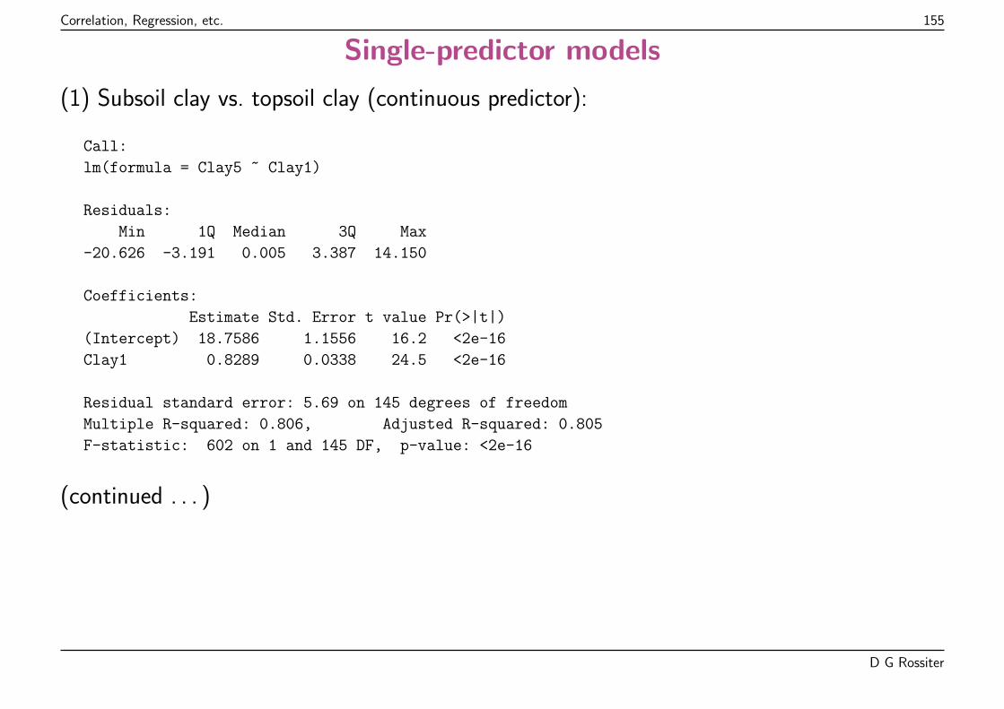
Correlation, Regression, etc. 155
Single-predictor models
(1) Subsoil clay vs. topsoil clay (continuous predictor):
Call:
lm(formula = Clay5 ~ Clay1)
Residuals:
Min 1Q Median 3Q Max
-20.626 -3.191 0.005 3.387 14.150
Coefficients:
Estimate Std. Error t value Pr(>|t|)
(Intercept) 18.7586 1.1556 16.2 <2e-16
Clay1 0.8289 0.0338 24.5 <2e-16
Residual standard error: 5.69 on 145 degrees of freedom
Multiple R-squared: 0.806, Adjusted R-squared: 0.805
F-statistic: 602 on 1 and 145 DF, p-value: <2e-16
(continued . . . )
D G Rossiter
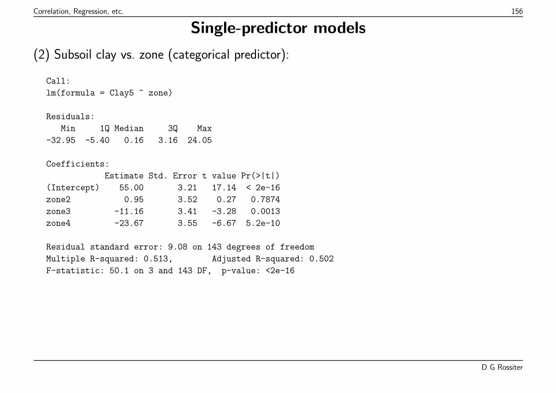
Correlation, Regression, etc. 156
Single-predictor models
(2) Subsoil clay vs. zone (categorical predictor):
Call:
lm(formula = Clay5 ~ zone)
Residuals:
Min 1Q Median 3Q Max
-32.95 -5.40 0.16 3.16 24.05
Coefficients:
Estimate Std. Error t value Pr(>|t|)
(Intercept) 55.00 3.21 17.14 < 2e-16
zone2 0.95 3.52 0.27 0.7874
zone3 -11.16 3.41 -3.28 0.0013
zone4 -23.67 3.55 -6.67 5.2e-10
Residual standard error: 9.08 on 143 degrees of freedom
Multiple R-squared: 0.513, Adjusted R-squared: 0.502
F-statistic: 50.1 on 3 and 143 DF, p-value: <2e-16
D G Rossiter
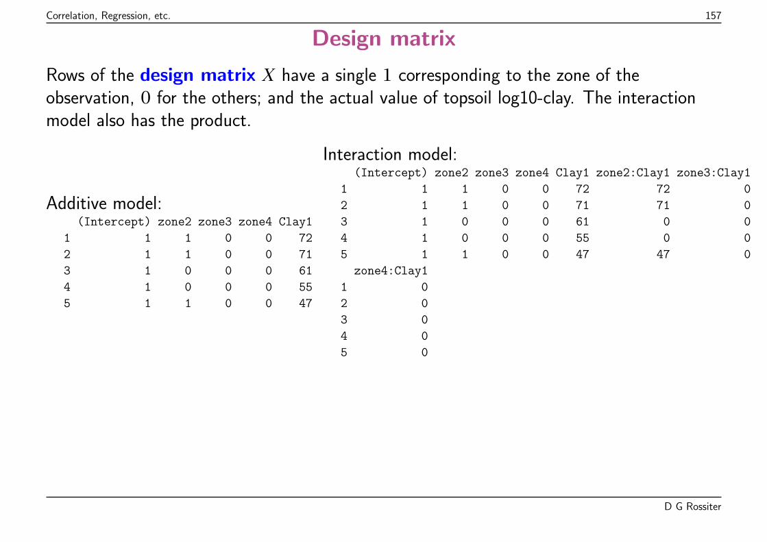
Correlation, Regression, etc. 157
Design matrix
Rows of the design matrix X have a single 1 corresponding to the zone of theobservation, 0 for the others; and the actual value of topsoil log10-clay. The interactionmodel also has the product.
Additive model:(Intercept) zone2 zone3 zone4 Clay1
1 1 1 0 0 72
2 1 1 0 0 71
3 1 0 0 0 61
4 1 0 0 0 55
5 1 1 0 0 47
Interaction model:(Intercept) zone2 zone3 zone4 Clay1 zone2:Clay1 zone3:Clay1
1 1 1 0 0 72 72 0
2 1 1 0 0 71 71 0
3 1 0 0 0 61 0 0
4 1 0 0 0 55 0 0
5 1 1 0 0 47 47 0
zone4:Clay1
1 0
2 0
3 0
4 0
5 0
D G Rossiter
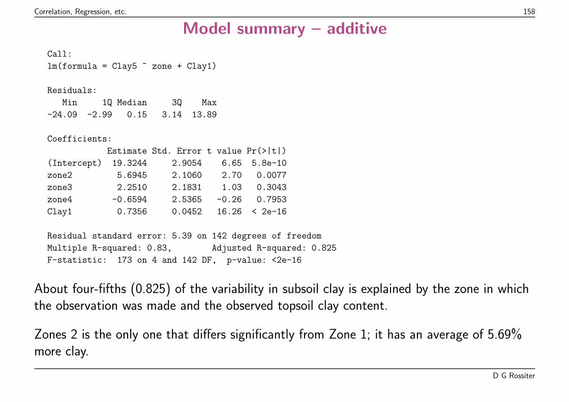
Correlation, Regression, etc. 158
Model summary – additive
Call:
lm(formula = Clay5 ~ zone + Clay1)
Residuals:
Min 1Q Median 3Q Max
-24.09 -2.99 0.15 3.14 13.89
Coefficients:
Estimate Std. Error t value Pr(>|t|)
(Intercept) 19.3244 2.9054 6.65 5.8e-10
zone2 5.6945 2.1060 2.70 0.0077
zone3 2.2510 2.1831 1.03 0.3043
zone4 -0.6594 2.5365 -0.26 0.7953
Clay1 0.7356 0.0452 16.26 < 2e-16
Residual standard error: 5.39 on 142 degrees of freedom
Multiple R-squared: 0.83, Adjusted R-squared: 0.825
F-statistic: 173 on 4 and 142 DF, p-value: <2e-16
About four-fifths (0.825) of the variability in subsoil clay is explained by the zone in whichthe observation was made and the observed topsoil clay content.
Zones 2 is the only one that differs significantly from Zone 1; it has an average of 5.69%more clay.
D G Rossiter
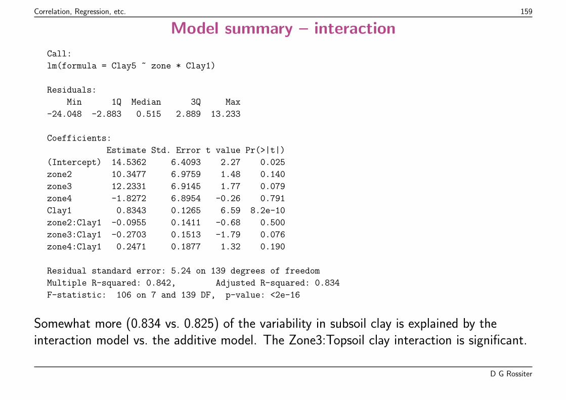
Correlation, Regression, etc. 159
Model summary – interaction
Call:
lm(formula = Clay5 ~ zone * Clay1)
Residuals:
Min 1Q Median 3Q Max
-24.048 -2.883 0.515 2.889 13.233
Coefficients:
Estimate Std. Error t value Pr(>|t|)
(Intercept) 14.5362 6.4093 2.27 0.025
zone2 10.3477 6.9759 1.48 0.140
zone3 12.2331 6.9145 1.77 0.079
zone4 -1.8272 6.8954 -0.26 0.791
Clay1 0.8343 0.1265 6.59 8.2e-10
zone2:Clay1 -0.0955 0.1411 -0.68 0.500
zone3:Clay1 -0.2703 0.1513 -1.79 0.076
zone4:Clay1 0.2471 0.1877 1.32 0.190
Residual standard error: 5.24 on 139 degrees of freedom
Multiple R-squared: 0.842, Adjusted R-squared: 0.834
F-statistic: 106 on 7 and 139 DF, p-value: <2e-16
Somewhat more (0.834 vs. 0.825) of the variability in subsoil clay is explained by theinteraction model vs. the additive model. The Zone3:Topsoil clay interaction is significant.
D G Rossiter
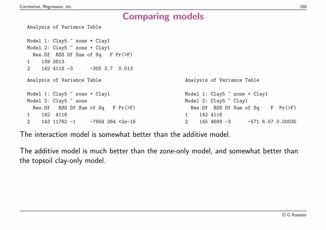
Correlation, Regression, etc. 160
Comparing modelsAnalysis of Variance Table
Model 1: Clay5 ~ zone * Clay1
Model 2: Clay5 ~ zone + Clay1
Res.Df RSS Df Sum of Sq F Pr(>F)
1 139 3813
2 142 4118 -3 -305 3.7 0.013
Analysis of Variance Table
Model 1: Clay5 ~ zone + Clay1
Model 2: Clay5 ~ zone
Res.Df RSS Df Sum of Sq F Pr(>F)
1 142 4118
2 143 11782 -1 -7664 264 <2e-16
Analysis of Variance Table
Model 1: Clay5 ~ zone + Clay1
Model 2: Clay5 ~ Clay1
Res.Df RSS Df Sum of Sq F Pr(>F)
1 142 4118
2 145 4689 -3 -571 6.57 0.00035
The interaction model is somewhat better than the additive model.
The additive model is much better than the zone-only model, and somewhat better thanthe topsoil clay-only model.
D G Rossiter
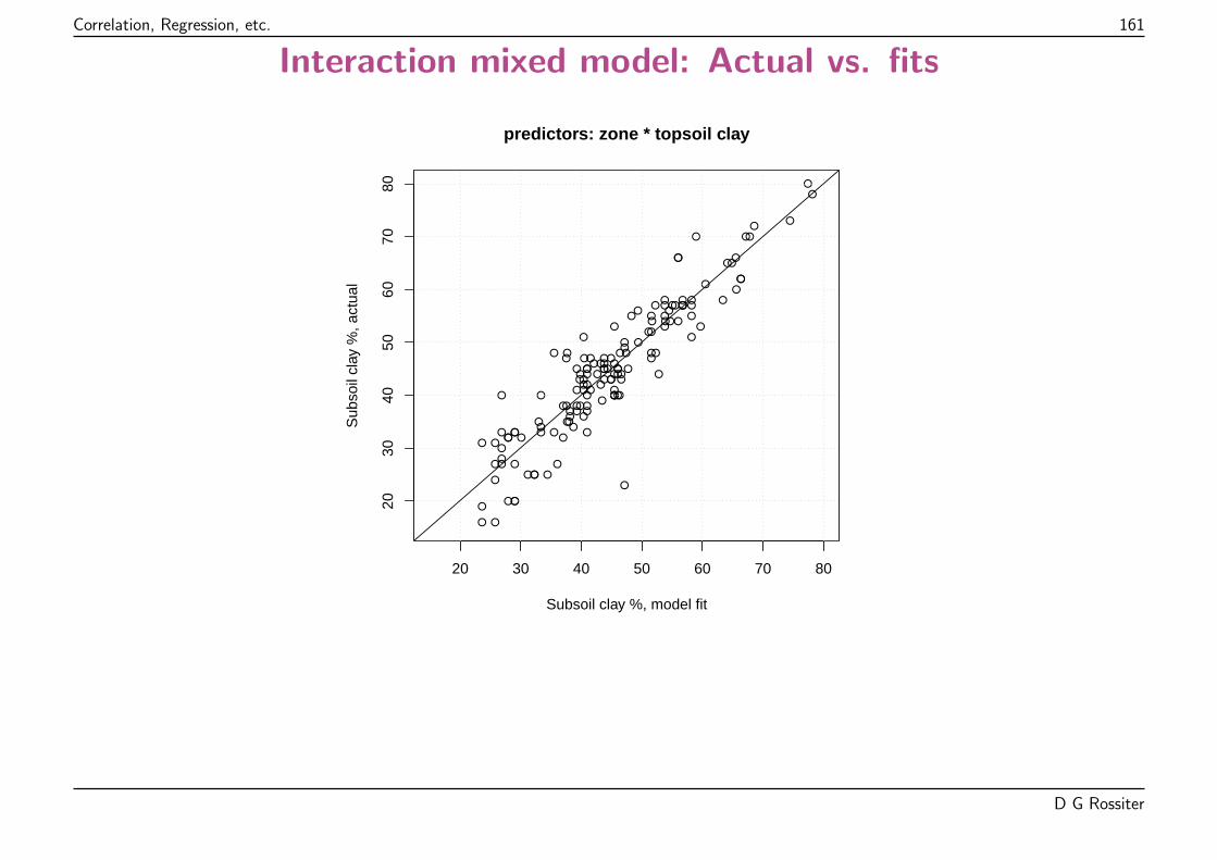
Correlation, Regression, etc. 161
Interaction mixed model: Actual vs. fits
●●
●
●
●
●
●●
●
●
●
●●
●●
●
●
●
●
●
●
●
●
●
●●
●
●
●
●● ●
●
●
●
●●
●
●
●
●
●
●
●
●
●
●
●
●
●
●
●
●
●
● ●●
●●●
●●
●
●
●●
●●
●
●
●
●
●
●
●●
●
●●●
●
●
●
●
●●●
●
●
●
●
●●
●●
●
●
●●
●●
●●
●
●
●
●●
●
●
●
●
●
●
●
●
●
●
●
●
●
●
●
●
●
●●
●
●
●●
●●
●
●
●
●
●
●
●●
●
●
●
●
●●
20 30 40 50 60 70 80
2030
4050
6070
80
predictors: zone * topsoil clay
Subsoil clay %, model fit
Sub
soil
clay
%, a
ctua
l
D G Rossiter
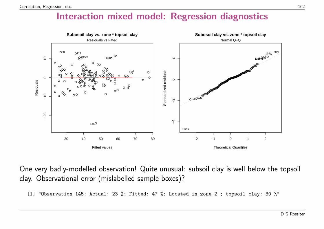
Correlation, Regression, etc. 162
Interaction mixed model: Regression diagnostics
30 40 50 60 70 80
−20
−10
010
Subosoil clay vs. zone * topsoil clay
Fitted values
Res
idua
ls
●
●
●●
●
●●
●
●
●
●
●
●
●
●
●
●
●
●
●
●●●●
●
●
●
●
●
●
●
●
●●
●
●
●
●
●
●
●
●
●●
●
●
●●●
●
●
●
●
●
●
●
●
●●
●
●●
●
●
●●
●
●
●
●
●
●
●
●
●●
●
●
●
●
●
●
●
●
●●●
●
●
●
●
●●
●●●
●
●
●
●
●
●
●
●
●
●
●●
●●
●
● ●
●
●
●
●
●
●
●
●
●
●
●●
●
●
●
●
●●
●
●●
●
●
●
●
●
●
●
●
●●
●
●
●
Residuals vs Fitted
145
38 11992742 137139
●
●
●●
●
●
●●
●
●
●
●
●
●
●
●
●
●
●
●
●● ●
●
●
●
●
●
●
●
●
●
●●
●
●
●
●
●
●
●
●
●●
●
●
●●●
●
●
●
●
●
●
●
●
●●
●
●●
●
●
●●
●
●
●
●
●
●
●
●
●●
●
●
●
●
●
●
●
●
● ●●
●
●
●
●
●●
●●●
●
●
●
●
●
●
●
●
●
●
●●
●●
●
●●
●
●
●
●
●
●
●
●
●
●
●●
●
●
●
●
●●
●
●●●
●
●
●
●
●
●
●
●●
●
●
●
−2 −1 0 1 2
−4
−2
02
Subosoil clay vs. zone * topsoil clay
Theoretical Quantiles
Sta
ndar
dize
d re
sidu
als
Normal Q−Q
145
3811992742137139
One very badly-modelled observation! Quite unusual: subsoil clay is well below the topsoilclay. Observational error (mislabelled sample boxes)?
[1] "Observation 145: Actual: 23 %; Fitted: 47 %; Located in zone 2 ; topsoil clay: 30 %"
D G Rossiter
Correlation, Regression, etc. 163
Visualizing the additive model
Parallel regression
� same slope on continuous predictor
� different intercepts per category on categorical predictor.
Does not allow a different response per category, only a different level.
D G Rossiter
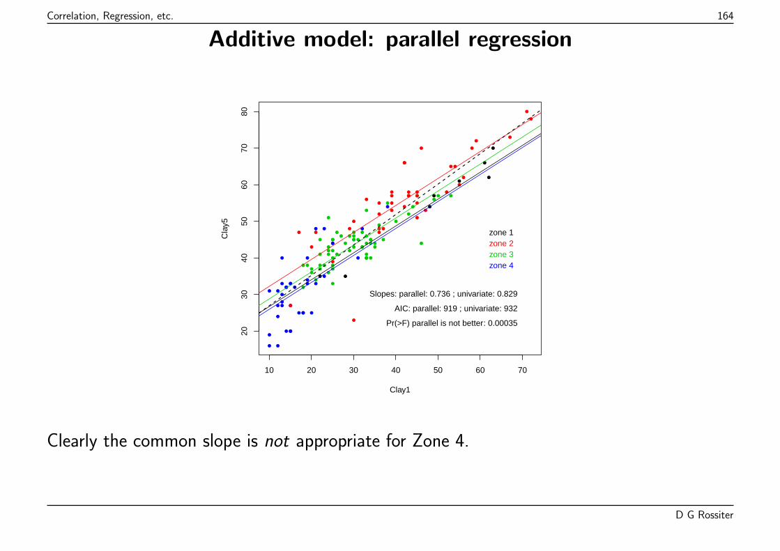
Correlation, Regression, etc. 164
Additive model: parallel regression
●
●
●
●
●
●
●
●
●
●
●
●●
●●
●
●
●
●
●
●
●
●
●
●
●
●
●
●
●
● ●
●
●
●
●●
●
●
●
●
●
●
●
●
●
●
●
●
●
●
●
●
●
● ●●
●●●
●●
●
●
●●
●
●
●
●
●
●
●
●
●●
●
●●●
●
●
●
●
● ●
●
●
●
●
●
●●
●
●
●
●
●
●
●
●
●●
●
●
●
●●
●
●
●
●
●
●
●
●
●
●
●
●
●
●
●
●
●
●●
●
●
●●
●
●
●
●
●
●
●
●
●
●
●
●
●
●
●●
10 20 30 40 50 60 70
2030
4050
6070
80
Clay1
Cla
y5
Slopes: parallel: 0.736 ; univariate: 0.829
AIC: parallel: 919 ; univariate: 932
Pr(>F) parallel is not better: 0.00035
zone 1zone 2zone 3zone 4
Clearly the common slope is not appropriate for Zone 4.
D G Rossiter
Correlation, Regression, etc. 165
Visualizing the interaction model
Non-parallel regression
� may have different slopes on continuous predictor, per category
� different intercepts per category.
Allows different responses per category, and different levels.
D G Rossiter
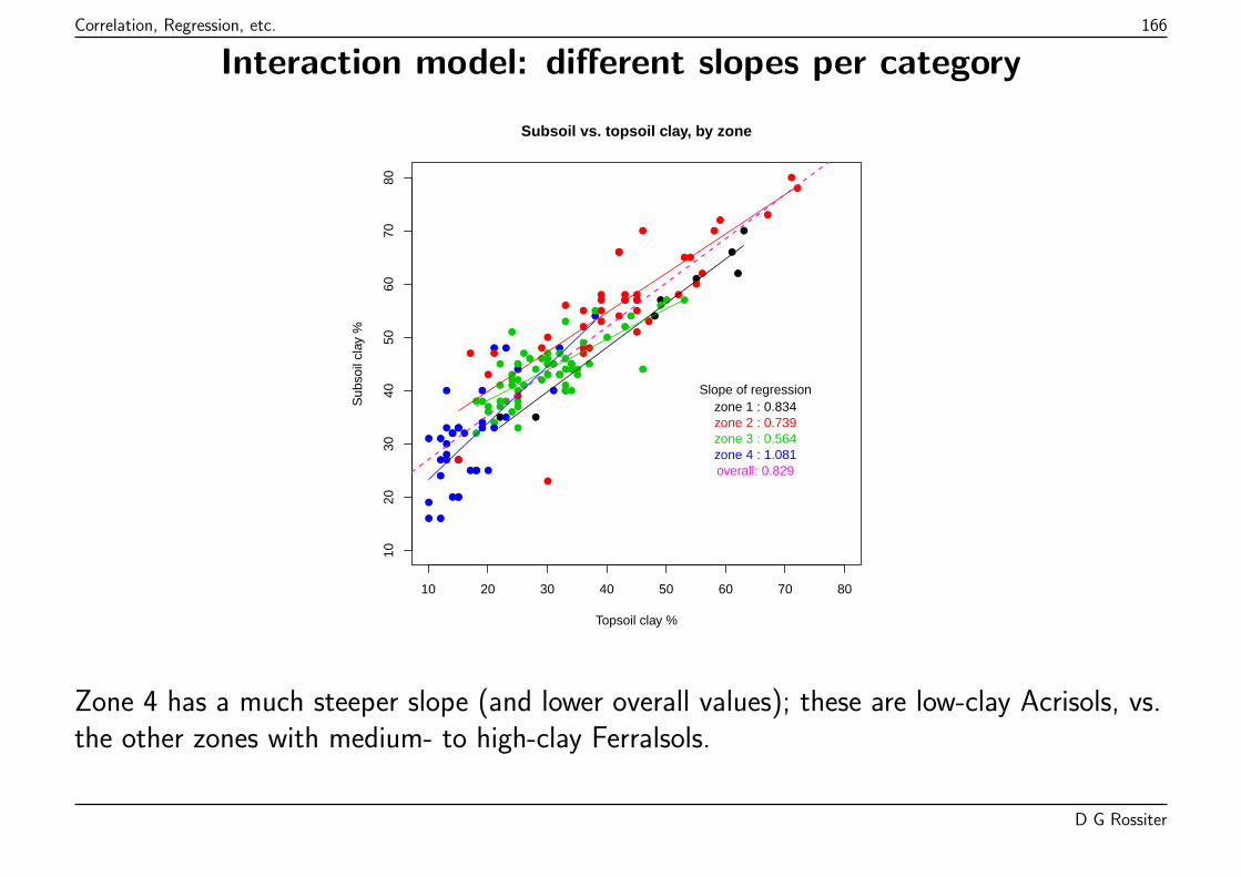
Correlation, Regression, etc. 166
Interaction model: different slopes per category
●
●
●
●
●
●
●
●
●
●
●
●●
●●
●
●
●
●
●
●
●
●
●
●
●
●
●
●
●
● ●
●
●
●
●●
●
●
●
●
●
●
●
●
●
●
●
●
●
●
●
●
●
● ●●
●●●
●●
●
●
●●
●
●
●
●
●
●
●
●
●●
●
●●●
●
●
●
●
● ●
●
●
●
●
●
●●
●
●
●
●
●
●
●
●
●●
●
●
●
●●
●
●
●
●
●
●
●
●
●
●
●
●
●
●
●
●
●
●●
●
●
●●
●
●
●
●
●
●
●
●
●
●
●
●
●
●
●●
10 20 30 40 50 60 70 80
1020
3040
5060
7080
Topsoil clay %
Sub
soil
clay
%
Subsoil vs. topsoil clay, by zone
Slope of regressionzone 1 : 0.834zone 2 : 0.739zone 3 : 0.564zone 4 : 1.081overall: 0.829
Zone 4 has a much steeper slope (and lower overall values); these are low-clay Acrisols, vs.the other zones with medium- to high-clay Ferralsols.
D G Rossiter
Correlation, Regression, etc. 167
Topic: Robust methods
If the assumptions of linear regression are violated, what do we do?
1. Violations of linearity: linearize, or non-linear methods
2. Residuals not normally-distributed, dependence of residual on fit
(a) Non-linearity: see above(b) A few poorly-modelled observations; especially high leverage (influential):
robust methods.
3. Variance differs across the range: heteroscedascity: variance-stabilizingtransformation
4. Not a single relation through the range: piecewise or local regression
Robust or resistant methods: good performance even if contamination from anotherprocess.
D G Rossiter
Correlation, Regression, etc. 168
Robust regression
This fits a regression to the“good”observations in a dataset.
The regression estimator has a high breakdown point: how many “bad” points there haveto be to distort the equation.
There are many options; here we use the default for the lqs function of the MASS Rpackage.
Reference: Venables, W. N., & Ripley, B. D. (2002). Modern applied statistics with S(Fourth ed.). New York: Springer-Verlag.
D G Rossiter
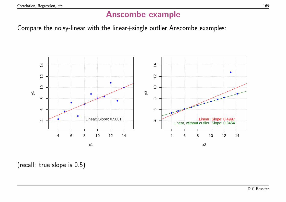
Correlation, Regression, etc. 169
Anscombe example
Compare the noisy-linear with the linear+single outlier Anscombe examples:
●
●
●
●
●
●
●
●
●
●
●
4 6 8 10 12 14
46
810
1214
x1
y1
Linear: Slope: 0.5001
●
●
●
●
●
●
●
●
●
●
●
4 6 8 10 12 14
46
810
1214
x3y3
Linear: Slope: 0.4997Linear, without outlier: Slope: 0.3454
(recall: true slope is 0.5)
D G Rossiter
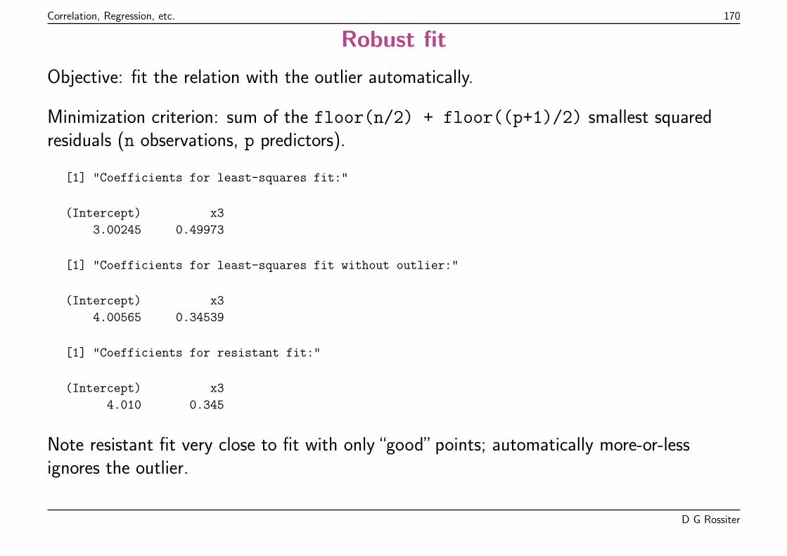
Correlation, Regression, etc. 170
Robust fit
Objective: fit the relation with the outlier automatically.
Minimization criterion: sum of the floor(n/2) + floor((p+1)/2) smallest squaredresiduals (n observations, p predictors).
[1] "Coefficients for least-squares fit:"
(Intercept) x3
3.00245 0.49973
[1] "Coefficients for least-squares fit without outlier:"
(Intercept) x3
4.00565 0.34539
[1] "Coefficients for resistant fit:"
(Intercept) x3
4.010 0.345
Note resistant fit very close to fit with only “good” points; automatically more-or-lessignores the outlier.
D G Rossiter
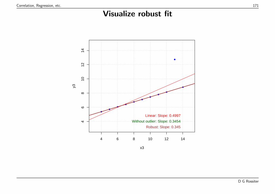
Correlation, Regression, etc. 171
Visualize robust fit
●
●
●
●
●
●
●
●
●
●
●
4 6 8 10 12 14
46
810
1214
x3
y3
Linear: Slope: 0.4997
Without outlier: Slope: 0.3454
Robust: Slope: 0.345
D G Rossiter
Correlation, Regression, etc. 172
Local regression
All the methods presented so far assume one relation (linear or otherwise) over the entirerange of the predictor.
Another possibility is local regression: fitting in pieces.
Many methods, with variable amounts of smoothing based on the span, i.e. theproportion of the range to consider for each piece.
Here we use the default for the lowess function of the R stats package, which usesiterated weighted least squares.
D G Rossiter
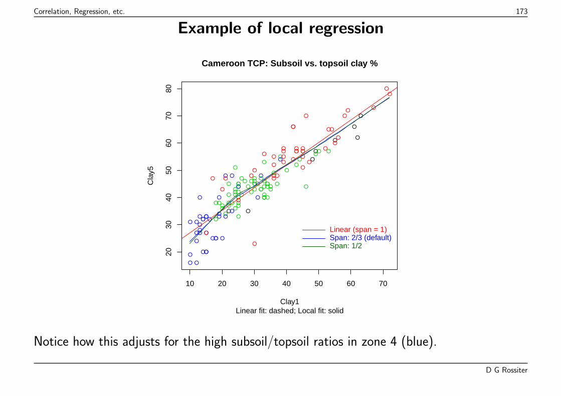
Correlation, Regression, etc. 173
Example of local regression
●●
●
●
●
●
●●
●
●
●
●●
●●
●
●
●
●
●
●
●
●
●
●●
●
●
●
●● ●
●
●
●
●●
●
●
●
●
●
●
●
●
●
●
●
●
●
●
●
●
●
● ●●
●●●
●●
●
●
●●
●●
●
●
●
●
●
●
●●
●
●●●
●
●
●
●
● ●●
●
●
●
●
●●
●●
●
●
●●
●●
●●
●
●
●
●●
●
●
●
●
●
●
●
●
●
●
●
●
●
●
●
●
●
●●
●
●
●●
●●
●
●
●
●
●
●
●●
●
●
●
●
●●
10 20 30 40 50 60 70
2030
4050
6070
80
Clay1
Cla
y5
Cameroon TCP: Subsoil vs. topsoil clay %
Linear fit: dashed; Local fit: solid
Linear (span = 1)Span: 2/3 (default)Span: 1/2
Notice how this adjusts for the high subsoil/topsoil ratios in zone 4 (blue).
D G Rossiter
Correlation, Regression, etc. 174
Conclusion
Modelling is not simple . . .
D G Rossiter