UNIVERSITEIT TWENTE

Correlating Features of Malicious

Software to Increase Insight in

Attribution

by

K.M. Beunder

A thesis submitted in partial fulfillment for the

degree of Master of Science

in the

Electrical Engineering, Mathematics and Computer Science (EEMCS/EWI)

Services, Cybersecurity and Safety (SCS)

August 2018

UNIVERSITEIT TWENTE

Abstract

Electrical Engineering, Mathematics and Computer Science (EEMCS/EWI)

Services, Cybersecurity and Safety (SCS)

Master of Science

by K.M. Beunder

This paper discusses research done on malware attribution: finding the author of a

malware sample. Attribution of malware is difficult and complex and with cyber crime

becoming more and more popular, law enforcement is facing an uphill battle.

Malware attribution is a complex problem. Unless the attacker makes a rookie mistake

and gives away his name and/or IP address it will be difficult and sometimes impossible

to determine who the author of a malware sample is (if there is a single author). Not

only is malware typically thoroughly stripped by its user (not always the author) of

any reference to its origin, malware is also likely to be obfuscated which complicates

any analysis procedure. Malware can also be equipped to evade analysis by detecting

specific environmental settings that are reminiscent of analysis.

This research consists of two parts. The first part experiments with the malware anal-

ysis tool Cuckoo Sandbox and different machine learning models to determine possible

attribution accuracy. The second part analyzes malware samples, both obfuscated and

non-obfuscated versions, to determine the effects of different obfuscation tools on the

analysis and the analysis results. Both static and dynamic behavior of the samples are

used in the analysis.

The results show that even when using only features from static analysis, accuracies

of up to 57% and 72% can be achieved. Furthermore obfuscation tools can have an

impact on both static and dynamic features although the simpler obfuscation tools only

influence the static ones.

It is argued that with more research this type of analysis will be useful to law enforcement

with respect to malware attribution. The usefulness will be limited to narrowing down

the “WHO question” by providing a list of possible suspects.

Acknowledgements

I want to thank my main supervisor, Dr. M.H. Everts, for his patience and guidance.

I am grateful to my second supervisor, Dr. A. Peter, for taking the time to review my

work. I also want to thank J.M. van Lenthe MSc for giving me some insight in the inner

workings of the High Tech Crime Unit.

Finally I want to thank a number of friends and family members for being patient with

me and helping me keep my spirits up especially during the difficult and stressful times.

ii

Contents

Abstract i

Acknowledgements ii

1 Introduction 1

1.1 Key Components . . . . . . . . . . . . . . . . . . . . . . . . . . . . . . . . 2

1.2 Summary of Contributions . . . . . . . . . . . . . . . . . . . . . . . . . . . 3

2 Malware 4

2.0.1 Threat Landscape . . . . . . . . . . . . . . . . . . . . . . . . . . . 4

2.0.2 Malware Attributes . . . . . . . . . . . . . . . . . . . . . . . . . . 5

2.0.3 Anti-Malware Measures . . . . . . . . . . . . . . . . . . . . . . . . 7

2.1 Malware Analysis . . . . . . . . . . . . . . . . . . . . . . . . . . . . . . . . 8

2.2 Anti-Analysis Measures . . . . . . . . . . . . . . . . . . . . . . . . . . . . 8

2.2.1 Obfuscation . . . . . . . . . . . . . . . . . . . . . . . . . . . . . . . 9

2.2.1.1 Packers . . . . . . . . . . . . . . . . . . . . . . . . . . . . 10

2.2.1.2 Cryptors . . . . . . . . . . . . . . . . . . . . . . . . . . . 11

2.2.1.3 Source Code Obfuscators . . . . . . . . . . . . . . . . . . 11

3 Related Work 12

3.1 Author Classification . . . . . . . . . . . . . . . . . . . . . . . . . . . . . . 12

3.2 Stylometry . . . . . . . . . . . . . . . . . . . . . . . . . . . . . . . . . . . 13

3.3 Malware Behavior . . . . . . . . . . . . . . . . . . . . . . . . . . . . . . . 14

3.4 Compiler Provenance . . . . . . . . . . . . . . . . . . . . . . . . . . . . . . 14

3.5 Memory Forensics . . . . . . . . . . . . . . . . . . . . . . . . . . . . . . . 15

4 Experimental Setup 17

4.1 Environment Setup . . . . . . . . . . . . . . . . . . . . . . . . . . . . . . . 17

4.1.1 Cuckoo Sandbox . . . . . . . . . . . . . . . . . . . . . . . . . . . . 18

4.1.2 Profiling Environment . . . . . . . . . . . . . . . . . . . . . . . . . 20

4.1.3 Testing Environment . . . . . . . . . . . . . . . . . . . . . . . . . . 20

4.1.4 Experiment 2 Adjustments . . . . . . . . . . . . . . . . . . . . . . 21

5 Experiment 1: Classification of real malware samples based on Cuckoofeatures 22

5.1 Sample Selection . . . . . . . . . . . . . . . . . . . . . . . . . . . . . . . . 23

5.2 Experiment Architecture . . . . . . . . . . . . . . . . . . . . . . . . . . . . 23

iii

Contents iv

5.2.1 Sample Submission . . . . . . . . . . . . . . . . . . . . . . . . . . . 24

5.2.2 Feature Extraction . . . . . . . . . . . . . . . . . . . . . . . . . . . 24

5.2.2.1 Type Features . . . . . . . . . . . . . . . . . . . . . . . . 25

5.2.2.2 String Features . . . . . . . . . . . . . . . . . . . . . . . . 25

5.2.2.3 Complete Feature Set . . . . . . . . . . . . . . . . . . . . 26

5.2.3 Machine Learning . . . . . . . . . . . . . . . . . . . . . . . . . . . 27

5.2.3.1 K-Nearest Neighbors . . . . . . . . . . . . . . . . . . . . 29

5.2.3.2 Decision Tree . . . . . . . . . . . . . . . . . . . . . . . . . 30

5.2.3.3 Random Forest . . . . . . . . . . . . . . . . . . . . . . . . 30

5.2.3.4 Neural Network . . . . . . . . . . . . . . . . . . . . . . . 30

5.2.3.5 Modeling the String Features . . . . . . . . . . . . . . . . 31

5.3 Results . . . . . . . . . . . . . . . . . . . . . . . . . . . . . . . . . . . . . . 32

5.3.1 Model Comparison . . . . . . . . . . . . . . . . . . . . . . . . . . . 32

5.3.2 Analysis of Authors . . . . . . . . . . . . . . . . . . . . . . . . . . 33

6 Experiment 2: Obfuscation and information loss in Cuckoo reports 36

6.1 Sample Selection . . . . . . . . . . . . . . . . . . . . . . . . . . . . . . . . 36

6.2 Sample Preparation . . . . . . . . . . . . . . . . . . . . . . . . . . . . . . 37

6.2.1 Packers . . . . . . . . . . . . . . . . . . . . . . . . . . . . . . . . . 38

6.2.1.1 UPX . . . . . . . . . . . . . . . . . . . . . . . . . . . . . 38

6.2.1.2 Themida . . . . . . . . . . . . . . . . . . . . . . . . . . . 38

6.2.2 Source Code Obfuscator . . . . . . . . . . . . . . . . . . . . . . . . 39

6.3 Experiment Architecture . . . . . . . . . . . . . . . . . . . . . . . . . . . . 39

6.3.1 Sample Submission . . . . . . . . . . . . . . . . . . . . . . . . . . . 40

6.3.2 Report Analysis . . . . . . . . . . . . . . . . . . . . . . . . . . . . 40

6.4 Results . . . . . . . . . . . . . . . . . . . . . . . . . . . . . . . . . . . . . . 40

6.4.1 Manual Reports Analysis . . . . . . . . . . . . . . . . . . . . . . . 41

6.4.2 Info Points . . . . . . . . . . . . . . . . . . . . . . . . . . . . . . . 44

7 Evaluation & Discussion 45

7.1 Experiment 1 . . . . . . . . . . . . . . . . . . . . . . . . . . . . . . . . . . 45

7.1.0.1 Feature Importance . . . . . . . . . . . . . . . . . . . . . 47

7.1.0.2 Author-specific Statistics . . . . . . . . . . . . . . . . . . 47

7.1.1 Reflection . . . . . . . . . . . . . . . . . . . . . . . . . . . . . . . . 48

7.2 Experiment 2 . . . . . . . . . . . . . . . . . . . . . . . . . . . . . . . . . . 49

7.2.1 Reflection . . . . . . . . . . . . . . . . . . . . . . . . . . . . . . . . 50

7.3 Discussion . . . . . . . . . . . . . . . . . . . . . . . . . . . . . . . . . . . . 51

8 Conclusion & Future Research 53

8.1 Future Research . . . . . . . . . . . . . . . . . . . . . . . . . . . . . . . . 53

8.1.1 Sample Database . . . . . . . . . . . . . . . . . . . . . . . . . . . . 54

8.1.2 Tool Environment . . . . . . . . . . . . . . . . . . . . . . . . . . . 55

8.1.3 Machine Learning . . . . . . . . . . . . . . . . . . . . . . . . . . . 55

A Simple Encoding Schemes 57

A.1 Base64 . . . . . . . . . . . . . . . . . . . . . . . . . . . . . . . . . . . . . . 57

Contents v

A.2 XOR . . . . . . . . . . . . . . . . . . . . . . . . . . . . . . . . . . . . . . . 57

A.3 ROT13 . . . . . . . . . . . . . . . . . . . . . . . . . . . . . . . . . . . . . 58

B Classifier Implementations 59

B.1 K-Nearest Neighbors . . . . . . . . . . . . . . . . . . . . . . . . . . . . . . 59

B.2 Decision Tree . . . . . . . . . . . . . . . . . . . . . . . . . . . . . . . . . . 60

B.3 Random Forest . . . . . . . . . . . . . . . . . . . . . . . . . . . . . . . . . 60

B.4 Neural Network . . . . . . . . . . . . . . . . . . . . . . . . . . . . . . . . . 60

C Experiment 1 - Feature Importances 61

D Accuracies per Author 63

E Google Code Jam Samples 68

F Cuckoo Report 69

G Results Experiment 2 77

Bibliography 79

Chapter 1

Introduction

Digital crime has become an increasingly popular form of crime over the past years. It

is a crime you can commit while sitting in the comforts of your home, with a large pool

of victims since a fair part of our lives is digital. Moreover, learning the necessary skills

has become easy, with some help from the internet.

As with every type of crime, the main question law enforcement wants answered is: who

is responsible? Or, to whom can this crime be attributed? A digital crime has a digital

crime scene (for the most part) and requires certain expertise to analyze. There are dif-

ferent types of digital crime, one of those and the one on which this research will focus,

is malware. Basically malware is software written for malicious reasons. In this research

we focus on malware, for which malware or malware-like samples can be collected and

of which it would be interesting to analyze the contents for clues related to the author.

It is worth mentioning that in the case of malware, the attacker/perpetrator and the

author of the malware are not necessarily the same person. Just like a shooter and the

maker of the gun do not have to be the same person.

Several quotes from the book Countdown to Zeroday [1], a book on the discovery and

dissection of Stuxnet, show that malware attribution is a problem that even the most

experienced professionals encounter and sometimes have insurmountable problems in

solving:

“Attribution is an enduring problem when it comes to forensic investigations of hack

attacks. Computer attacks can be launched from anywhere in the world and routed

through multiple hijacked machines or proxy servers to hide evidence of their source.

Unless a hacker is sloppy about hiding his tracks, it’s often not possible to unmask the

perpetrator through digital evidence alone.”

1

Introduction 2

“But sometimes malware writers drop little clues in their code, intentional or not, that

can tell a story about who they are and where they come from, if not identify them

outright. Quirky anomalies or footprints left behind in seemingly unrelated viruses or

trojan horses often help forensic investigations tie families of malware together and

even trace them to a common author, the way a serial killer’s modus operandi links

him to a string of crimes.”

Finding the responsible party of malware is an ongoing subject of interest. There are

already several research papers in existence on the subject, although most of these do

not use real malware samples but mock-malware samples for the evaluation. The use of

mock-malware samples is usually for the simple reason that it is difficult to find a large

set of real malware samples with any identifiable information on the authors.

What can complicate the analysis of malware is the use of obfuscation by the author.

Obfuscation can be used to distort some potentially identifying features.

The analysis of malware can be further complicated if an author uses some form of ob-

fuscation on the malware. Obfuscation can distort some potentially identifying features

in the malware, which most authors will do to some extent.

1.1 Key Components

The main issue we want to investigate in this research is whether automatic malware

attribution could be a reliable supporting system for example for law enforcement. So

the main question is:

Can automatic malware attribution be useful in an investigation to identify the author?

This question is split into two sub questions that we intend to answer, thereby trying to

piece together an answer to our main question.

• Can automatic malware attribution be reliable enough such that it can contribute

to an investigation?

• What are the effects of obfuscation on any features, and their content, that can

be extracted from malware?

We will explore two aspects of malware analysis. One of the aspects is the classification

of malware samples, based on the features which form the author profile. The other is

the effect of obfuscation on the extraction of features from malware samples.

Introduction 3

The same setup can be used for both experiments, with a virtual machine were the

malware samples can be run and analyzed. In the first experiment real malware samples

are analyzed and using machine learning we try to determine how accurately the samples

can be classified according to author. In the second experiment features are extracted

from mock-malware samples, some of which are obfuscated, allowing for a comparison

of the type of features that can be extracted and how much information they contain.

1.2 Summary of Contributions

The next chapter starts with some basic knowledge on malware to help understand the

different components and terms used in the rest of the paper. This is followed by a

chapter on previous research that has been done in the same area as this research, which

gives some interesting insights as to how malware analysis can be approached.

Chapter 4 explains how the environment in which the experiments will be executed is

setup and the process driving the configuration of the environment. After this chapter

on the setup for the experiments, two chapters follow, each dedicated to one of the exper-

iments. The experiment chapters describe what samples are used, how the experiment

is constructed (what steps are taken), and ends with the results. The chapter after the

two experiment chapters evaluates the results for each of the experiments. The thesis

ends with the conclusion of this research.

Chapter 2

Malware

Malware, short for malicious software, is any software designed to cause detriment to

a user, computer, network or equipement/machinery/etc. connected to the computer

and/or network. There are many types of malware including Trojan horses, back-

doors, worms, downloaders, bots, spyware, adware, fake antiviruses, rootkits, file in-

fector viruses, and the current newest addition, ransomware [2]. Malware can be a

combination of these types since some types are more focused on the infiltration of a

computer system, some on the way the malware replicates and spreads, and others on

staying hidden once it has infected a system. So for example one piece of malware may

fall in the three categories of the fake antivirus, rootkit, and spyware. Using the fake

antivirus angle to get access to a system, hiding itself like a rootkit, and gathering user

information like spyware.

2.0.1 Threat Landscape

There are three main types of attackers: those in it for financial gain, hacktivists who are

motivated by political issues, and nation states which is nation hacking other nations.

Of these three types financial gain is often the motivation behind the malware, like Cryp-

toLocker (ransomware) where a victim’s files are encrypted rendering them unusable to

the user and decryption is offered in exchange for payment of the ransom.

An example of hacktivists is the group Anonymous that for example has executed sev-

eral DDoS (Distributed Denial of Service) attacks against different governments and

corporations.

There are also cases where nations attack other nations. Usually this means a nation’s

military and/or intelligence arm, or hired individuals or teams, hacking another nation’s

assets (like companies, critical infrastructure, government officials, etc.). These cases are

inherently more complex given a nation’s resources and the precautions they are willing

4

Malware 5

to take to hide their involvement. Some nations might regard “being hacked” as an act

of war. These types of cases are very hard to prove. An example is the Stuxnet worm,

which was most likely an American-Israeli creation (although neither country admitted

to this) that very specifically sabotaged certain components that were in use by Iran’s

nuclear facility thereby delaying the Iranian nuclear program.

You might expect the culprit behind a malware attack to be an expert with a computer

and the knowledge to craft malware. However, if you know where to look, there are

markets for malware where one can simply purchase different malware components, no

special skills required. This concept is known as Malware-as-a-Service (MaaS) and is

part of the cyber black market. All sorts of malware related services can be found in this

market. Among other things you can find malware components or complete packages,

ransomware is a popular product, and botnets can be hired to do a DDoS attack. Such

a market, where malware could simply be bought, allows just about anybody to become

a cyber criminal.

This has a number of major consequences. Since the threshold is lower, there are likely

to be more cyber criminals. The customer service in this market has also become

increasingly professional, further improving the accessibility. Second, for those who know

how to write the malware, they can sell their creations on the black market, making

money with substantially less risk because they are not the ones directly attacking

anybody. Another consequence could be that a lot of knowledge can be exchanged (this

mostly on fora) and different malware or malware techniques can be combined to make

more technical and complex attacks.

2.0.2 Malware Attributes

Before analyzing malware it can be helpful to know what characteristics malware can

possess.

Malware can come in different types of files, executables but also JAR files, some kinds

of script, shortcut files, macros (like .doc), etc.

Malware, like any software, can be written in many languages, the choice is the author’s.

Malware is often written in C or C++, middle level languages (see figure 2.1 for illus-

tration of code layers). Writing in an assembly language allows the author to do more

complex things, but assembly language is less readable to humans and significantly more

cumbersome to write, debug and maintain.

Depending on the target of the malware the author has to decide for which operating

system (OS) to write the malware. Servers, of businesses and like, often run a Linux

Malware 6

Figure 2.1: Flow of compilation and disassembly [3]

OS. However most regular consumers have laptops with Windows or Mac OS on it.

With Windows being the most used operating system, followed by the Mac OS after

Window’s huge head start, it is not all that surprising that most of the malware targets

Windows systems since that means more potential targets. Other reasons that may

makes Windows an appealing target are that Windows has a long history with many

compatibility requirements and there are many illegal copies in circulation which can

not be updated, leaving potential flaws exposed. Hackers’ interest in targeting the Mac

OS has been increasing of late [4]. Also mobile devices and their OSes have become an

interesting target since more and more mobile devices becoming more popular. Even

devices that one might not expect to be targeted could get infected, anything with a

small amount of storage, like your digital thermostat.

When writing code, programmers can import libraries to use existing code to facilitate

their program instead of writing everything themselves. Since different libraries are

used for different things, the imports of a file can help indicate what type of functions

the program needs which can give an indication as to what the program does. These

imported libraries and functions can be extracted for analysis, for a Windows executable

this would be listed in the program’s PE (portable executable) format.

The PE format is a file format that contains information that Windows OS loader needs

to manage the file. Executables, object code and DLLs for instance come in a PE file

format. The PE format consists of a header followed by several sections including the

program code. The header contains metadata like information on the code, the type

of application, required library functions, and space requirements. Malware meant for

Windows machines will also have the PE file format to be able to run and it might be

possible to get some useful information from the PE header.

Malware 7

Figure 2.2: Simple overview of the arrangement of a program in PE file format [5]

2.0.3 Anti-Malware Measures

There are several measures that can be taken to decrease the chance of a malware

infection.

Antivirus tools are popular and available both paid/subscribed and as freeware. The

name is based on times when the focus was mostly on viruses, nowadays however an-

tivirus companies have expanded to combat more than just viruses, but the term remains

the same. Unfortunately, antivirus programs are incapable of detecting and blocking all

malware. Traditional antivirus software depends on signatures stored in the antivirus

company’s database of malware signatures to identify malware. In this case a signature

is a unique value (like a hash), which is calculated from the malware, that identifies that

specific malware sample. When a new malware is encountered, the anti-virus company

must first add the signature of this new malware to its database for the anti-virus pro-

gram to be able to recognize it as malware. They cannot detect malware that is not

known to them.

There are also anti-malware products which are more focused on newer malware that

may be polymorphic (self-modifying) or make use of zero-days1, compared to antivirus

products which mainly deal with more traditional malware from traditional sources.

When installed antivirus and anti-malware hook themselves into the system, similar to

how some malware might do except with permission, and whenever the operating system

accesses a file the antivirus or anti-malware intervenes and first checks whether the file

is legitimate. If the file is flagged as malware, the accessing of the file is stopped (and

typically quarantined) and the user is warned.

1a vulnerability in soft-, firm-, or hardware that is unknown to the party responsible for the patchingor fixing of the vulnerability

Malware 8

Other examples of preventative measures are firewalls, website security scans, awareness

counseling and in extreme cases “air gap” isolation (no connections whatsoever, air all

around).

2.1 Malware Analysis

The analysis of malware is similar to other investigations. With the same basic ques-

tions: Who? What? Where? When? And why?

There are basically two forms of malware analysis, static and dynamic analysis. Static

analysis, also known as code analysis, is the analysis of the actual files/resources con-

taining the malware, which can be as basic as the extracting of any strings to be found

or as advanced as actually reverse engineering the binary. Basically everything you can

do without running the file.

Dynamic analysis, also known as behavioral analysis, is the analysis of behavior of a

running malware sample, for example the internet connections it tries to make, what

processes it creates, etc. Although it is prudent to use a safe environment for both types

of analysis, it is absolutely necessary for dynamic analysis because the malware is made

to execute in order to analyze it.

Static and dynamic analysis are comparable to the approaches of whiteboxing and black-

boxing used elsewhere (for example in this course on malware analysis [2]). Where

whiteboxing is the taking apart of the file itself as to inspect the inner workings and

blackboxing is the running of the malware and observing its behavior to determine what

changes it makes to the machine. Whiteboxing will often help us understand the why

and the who, while the blackboxing will often help with the what, when and where.

2.2 Anti-Analysis Measures

The analysis of malware can be hampered when anti-forensic techniques2 are included

in the malware. For any malware analysis technique, sooner or later a way to counter

or circumvent it is found. Just as new types of attacks will provoke the development of

new defenses against it. Not surprisingly this results in an endless cat and mouse game

of measure and counter-measure.

2Wikipedia says: anti-computer forensics is a general term for a set of techniques used as counter-measures to forensic analysis

Malware 9

Anti-forensics can be implemented using obfuscation3 techniques. There are several ob-

fuscation tools available online to facilitate this.

Another type of anti-forensic technique are the anti-virtual machine (anti-VM) tech-

niques. Virtual machines are useful environments to use for dynamic malware analysis

for several reasons. They are mostly meant as a closed off separate environment on a

host machine that acts as normal PC but can be viewed from the host machine for analy-

sis. Virtual machines are also easy to manage and clean. The state of a virtual machine

environment can be saved in a snapshot, to which the virtual machine can be reset,

reverting to a clean state after malware analysis. Or they can simply be deleted after

use. Anti-virtual machine techniques can result in the malware altering its functionality

or not running at all if it detects that it is being run in a virtual environment, defeating

the purpose of running the malware in the virtual environment. Another, non-cyber

specific, way of making analysis harder is to commit the crime with multiple people,

especially if the consistency of the group were to change often. If several programmers

instead of one programmer were to have worked on one piece of malware, they might be

obscuring each others identity if the malware is analyzed as a whole for attribution.

2.2.1 Obfuscation

Obfuscators were originally introduced to make it difficult to decode commercial code,

in particular C++, to avoid loss of intellectual property. Malware writers often use

obfuscation to hide their tracks. Obfuscation is mostly used to hide the purpose of the

malware. Depending on how much effort the creator puts into obfuscating the code, this

could result in additional work for anyone trying to analyze it. Obfuscation will at least

complicate the static analysis of the malware.

Tools for obfuscation can be classified under different names such as Packers, Cryptors

(encryption tools) or simply Obfuscators, depending on its technique. The most popular

type of obfuscation is packing. There are many such tools available, ranging in com-

plexity, and it is not unusual to encounter self-made tools. Some packers include options

like encryption, virtual-environment detection, etc. making lone cryptors somewhat

obsolete.

There are also forms of obfuscation that are not usually done with tools, but that are

simply diversion techniques built into the code. For instance having the executable wait

for a substantial amount of time before actually doing anything to give the illusion that

it is harmless.

3According to Google obfuscation is: the action of making something obscure, unclear, or unintelli-gible.

Malware 10

2.2.1.1 Packers

The packing of a file involves the compressing of the original file and inserting this into

a new executable with a small wrapper program. The wrapper program is responsible

for the unpacking when the packed program is executed. It extracts and decompresses

the original file into memory so the original file can be run. Due to the compression the

packed file takes up less space, with the additional property of making the payload less

easy to recognize or analyze.

There are many types of packers, each with there own packing algorithm; you can even

write your own. The packing algorithm defines how a file is compressed [6]. To unpack

a compressed file you need to know which algorithm was used to pack it or have the

correct tool to decompress the file.

The type of packers relevant to this research are runtime packers, which is the com-

pression of executables were the decompression occurs at runtime (when the packed

executable is run). These differ from packers like zip and rar in several ways. Zip and

rar for instance require certain type of tools/software to unpack, like 7Zip or WinRAR.

An executable compressed by a runtime packer has the decompression manual built in

as it were. It keeps the .exe extension and when executed unpacks itself in memory

to execute the original program. These compressed executables can also be called self-

extracting archives. If packed, malware is likely to be packed with a runtime packers

since malware is meant to remain executable.

Figure 2.3: The state of a program before and after compression (packing), and afterdecompression [7]

Originally packers were meant to make files smaller to use less disk space, and the self-

extracting meant that users wouldn’t have to manually unpack it themselves. However

with the current disk sizes and internet speeds these kind of measures aren’t required

anymore [8]. Nowadays a compressed executable is likely to be malware, although there

are very few packers that are used solely for malware [6]. The packing of the malware

can make it harder to detect, can complicate the reverse engineering and leaves a smaller

Malware 11

footprint on the victim’s machine as a bonus. To do any proper analysis the packer needs

to be unwrapped first.

2.2.1.2 Cryptors

The term cryptors sometimes refers to obfuscation tools, but can include actual en-

cryption which often makes it more complex, applying a transformation to make the

executable harder to detect [8]. Malware writers can choose to use simple ciphers to

encrypt their code, in which case they are just looking for an easy way of preventing

basic analysis from identifying their activities, or they can choose sophisticated ciphers

or even custom encryption, to make reverse engineering that much more difficult. En-

crypted programs will sometimes work in the same way as a packed program, with the

key instead of a decompression stub. Since the program needs to be able to run it needs

to be able to decrypt itself. In some cases the key may not be in the code somewhere, in

that case the malware will need to be given the order to run (by supplying the key) and

the owner of the malware will need some form of access to it to do this. Some simple

transformation examples may be the XOR (exclusive OR) cipher, Base64 encoding, and

ROT13. See Appendix A for more information on these ciphers. These are forms of

data encoding, which are key-less unlike encryption which always needs a key.

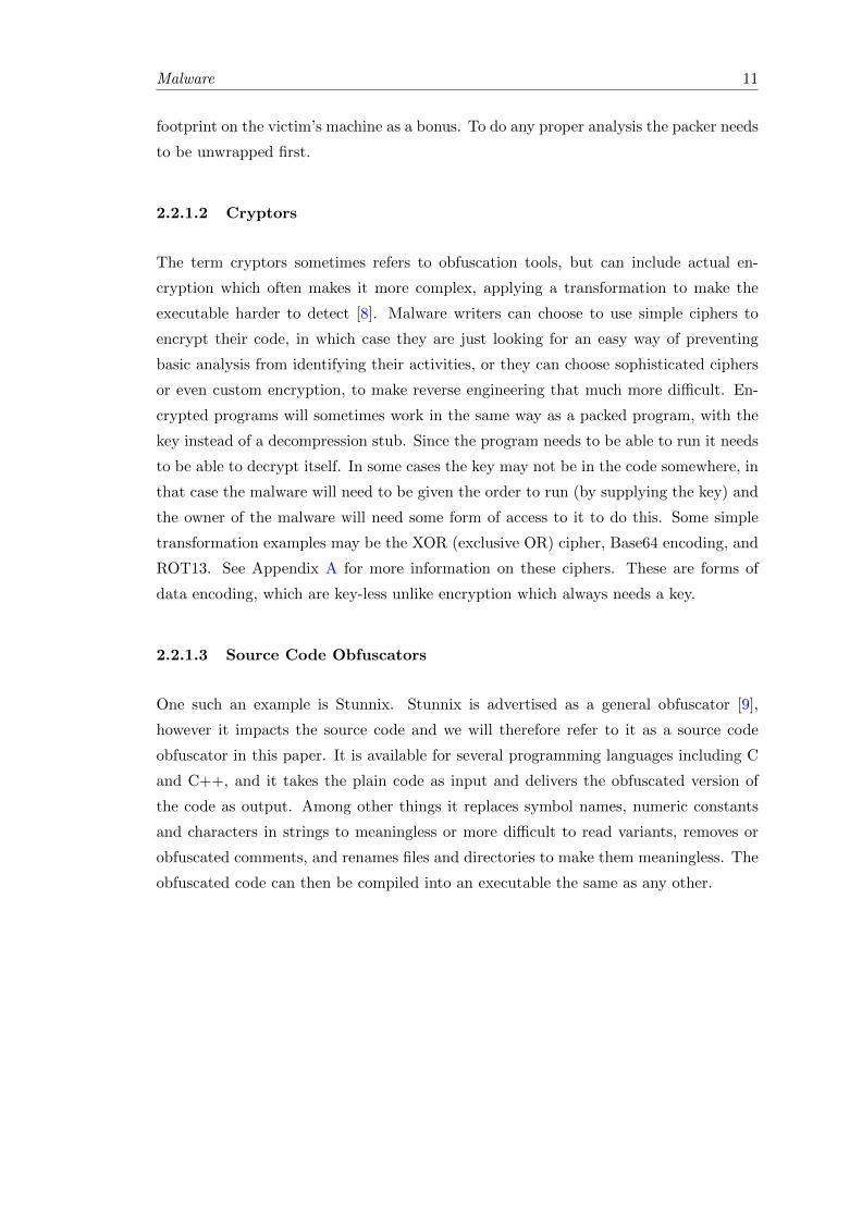
2.2.1.3 Source Code Obfuscators

One such an example is Stunnix. Stunnix is advertised as a general obfuscator [9],

however it impacts the source code and we will therefore refer to it as a source code

obfuscator in this paper. It is available for several programming languages including C

and C++, and it takes the plain code as input and delivers the obfuscated version of

the code as output. Among other things it replaces symbol names, numeric constants

and characters in strings to meaningless or more difficult to read variants, removes or

obfuscated comments, and renames files and directories to make them meaningless. The

obfuscated code can then be compiled into an executable the same as any other.

Chapter 3

Related Work

Malware analysis has been the focus of many research papers, some of which with

attribution as main focus. Malware attribution is deemed difficult because there is

a large body of potential authors to distinguish from, and finding fingerprints unique to

each specific author can be quite difficult. Not to mention the added degree of difficulty

when considering that (some parts of) a piece of software may be copied from elsewhere,

constructed by multiple authors or obfuscated in some way (remember for example MaaS

described in 2.0.1).

In research focused on author attribution we came across several papers that discuss

author classification of literary texts. Some aspects of the feature selection from literary

texts could be applicable in our own research. However it is expected that the content of

program will differ from any literary text, which is why we also examine research focused

specifically on author attribution of code. Two papers [10, 11] on this subject discuss

the use of stylometry features. Besides research specifically on author attribution, we

are also interested in other types of software (sometimes malware) analysis. Properties

of malware such as its behavior, which compiler was used and analysis of the malware

while in memory (memory forensics) can be considered as potentially useful features

in creating a fingerprint. A short discussions on each of these different aspects can be

found in the following sections.

3.1 Author Classification

Most author classification research is based on literary texts. To identify the author of a

text basically a kind of “fingerprint” is extracted from the text [12]. This fingerprint can

then be compared to other fingerprints from other texts. Since a fingerprint needs to be

12

Related Work 13

distinguishing in nature, meaning that the fingerprints of two different authors should

not be the same, it is important to use combination of features that makes conflicting

fingerprints unlikely.

There does not seem to be a consensus on which features produce the best results. A

possible categorization is lexical, syntactic, structural, content-specific, and idiosyncratic

style markers [13].

Using word frequencies to develop a fingerprint is a popular method. Other features

that might be used to characterize an author may be sentence length, word length,

abundance of vocabulary, etc. The features used by Elayidom et al. [12] include: number

of periods, of commas, of question marks, of colons, of blanks, of words, of sentences, of

characters, ratio of characters in a sentence, and top k word frequency. Specifically for

short messages Brocardo et al. [13] uses n-grams, investigating the n-gram sizes of 3, 4,

and 5.

3.2 Stylometry

Turning to attribution research specifically focused on the digital/code, two papers stand

out [10, 11]. In these papers attribution is investigated using stylometry features ex-

tracted from code. The first of these papers [10] indicates that stylometry features

extracted from source code are distinguishing and result in rather high accuracies (94%

and 98%). Three types of stylometry features are extracted from source code: lexical,

layout and syntactic. These features are merged into what they call the Code Stylome-

try Feature Set (CSFS). From the CSFS a smaller set of the most informative features

is extracted, and this set is used in a random forest classifier.

However in many (“real life”) cases access to the source code cannot be assumed. Which

leads to the follow-up research [11] in which stylometry features are extracted from

compiled samples. The results in this paper also indicate that stylometry features are

useful in distinguishing authors, resulting in almost equally high accuracies (up to 92%).

In this case the executables are disassembled and decompiled, during which features (like

raw instruction traces and symbol information) are extracted. Once disassembled and

decompiled the rest of the features, lexical and syntactic, are extracted. Here too the

feature set is reduced to a smaller set of the most informative features, using the same

method as in their previous research, after which it is used in a random forest classifier.

In both cases the number of distinctive authors used is limited, far smaller than the

amount of malware authors expected to be existent in “real life”. Although the method

analyzing source code appears to scale rather well, the question remains how effective

Related Work 14

code stylometry would be in real world situations. However the experiment results

suggest that stylometry features could help reduce the number of suspects when dealing

with attribution.

3.3 Malware Behavior

Research specific to malware and its classification seem to focus mainly on the behavioral

properties of the malware, like those extracted through dynamic analysis. Determining

the behavior of a malware sample means trying to determine what it is doing and maybe

also how. There are several aspects to examine for behavioral properties. One aspect to

analyze is what the malware itself is doing, like what functions it runs. Another aspect

is to analyze the environment for any changes that the malware may be responsible for,

like the creation of a file or registry. To analyze the changes to the environment, it is

easiest to run actually run the malware, preferably in some “safe” environment.

Two examples of research into malware behavior are the papers by Mohaisen et. al. and

Shang et. al. [14, 15]. The first of these two [14] describes the design of an analysis and

classification system they name AMAL. AMAL is a two part system, AutoMal which is

responsible for the analysis and MaLabel which does the classification and or clustering.

AutoMal analyzes files, registries, network behavior and memory dumps resulting in

features that MaLabel can use to distinguish between different variants within malware

families. The other paper [15] investigates the identification of malware by examining

the function calls found in the assembly code. The function calls are structured in a so-

called function-call graph as vertices and the directed and weighted edges represent the

calls made. Function-call graphs can be compared to each other to calculate similarity.

Although behavior properties are not likely to contain author specific information such

as a name or address, unless perhaps a message was left on purpose, they can help to

trace multiple samples back to a single origin. If the author of one of those samples can

be found it is likely he/she is also responsible for the others. Or perhaps the different

samples reveal different pieces of author information and the correlation can give a better

indication.

3.4 Compiler Provenance

Another possibly relevant aspect to consider is compiler provenance. This is any infor-

mation on the compiler, the compiler version and any other compiler settings with which

a program was compiled. In the research by Rahimian et al. [14] the created tool named

Related Work 15

BinComp uses syntactical, structural, and semantical features to recover compiler prove-

nance. Despite the fact that this tool assumes that any binaries to be analyzed are not

obfuscated or stripped and only certain types of architecture and programs are evalu-

ated, the authors conclude that their method and tool could be a practical approach

for real-world situations. While compiler provenance alone may not be enough for at-

tribution, as the authors of the paper say themselves it could be imperative to certain

applications, attribution among other things. It is after all the author who decides how

to compile his/her program.

3.5 Memory Forensics

A different way of analyzing the behavior of an executable is by studying it in memory

while it is being run. The advantage of inspecting a program in memory is that most

of the obfuscation is removed to run the executable and it is more robust against any

anti-forensic techniques [16]. The difficult part is finding it in memory once it is running.

There are several researches on memory forensics [16–18], each with their own approach

at finding, analyzing, and interpreting the program in memory.

One of the ways to access and retrieve properties of a program from memory, according

to Mosli et al. [16], is to use an automated tool like Cuckoo Sandbox [19]. It acquires

memory images and memory dumps, and can extract features, in this case registry

keys, imported DLLs, and API function calls. After obtaining the desired features, the

features are used in a number of different classification techniques are compared for the

different types of features. For the registry features the Stochastic Gradient Descent

performed best (with 96%). The classification techniques with the best performance for

the imported DLLs is the Random Forest (with 90,5%) and for the API function calls

it is the Stochastic Gradient Descent (with 93%).

Another memory forensic tool, focused mostly on how to find a sample in memory, is

presented with the HyperLink tool [17]. It tries to determine the programs placement in

memory without knowing the precise details of the kernel’s data structure. It assumes

that modern OSes organize key information in linked lists and that certain offsets are

a constant. Since a different OS version can mean a change in the kernel code, being

independent of these smaller changes can save time creating an update for each new OS

version. The cost of knowing less details means that only a portion of the information,

depending on properties that persist over different OS versions, is extracted from the

memory. It is stated that with the this partial information (the critical fiels) a process

list can be reconstructed.

Related Work 16

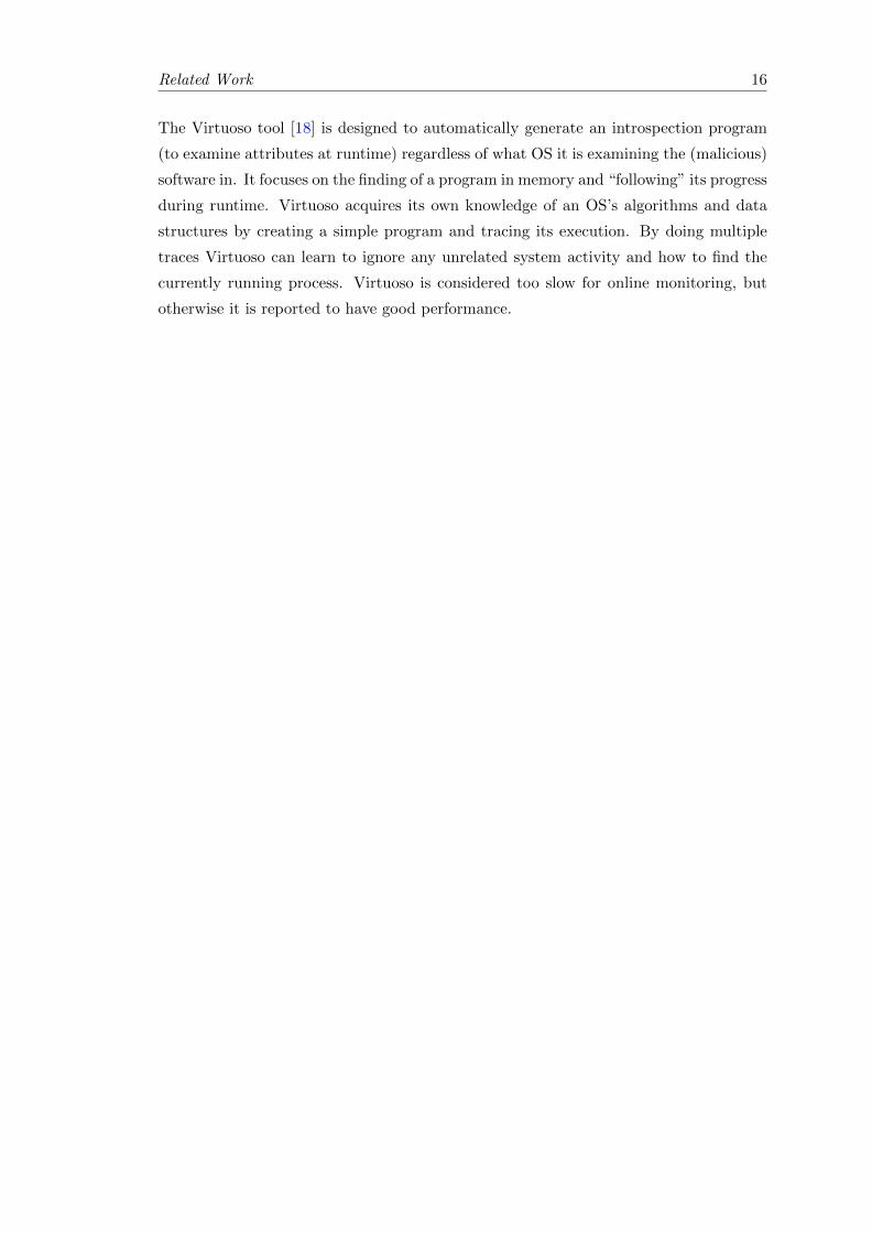
The Virtuoso tool [18] is designed to automatically generate an introspection program

(to examine attributes at runtime) regardless of what OS it is examining the (malicious)

software in. It focuses on the finding of a program in memory and “following” its progress

during runtime. Virtuoso acquires its own knowledge of an OS’s algorithms and data

structures by creating a simple program and tracing its execution. By doing multiple

traces Virtuoso can learn to ignore any unrelated system activity and how to find the

currently running process. Virtuoso is considered too slow for online monitoring, but

otherwise it is reported to have good performance.

Chapter 4

Experimental Setup

To explore the answers to the research questions introduced in the Introduction, two ex-

periments are performed. In the following two chapters the method of these experiments

is outlined, followed by a survey of the results.

Before starting on the experiments an environment for these experiments is set up. Since

the environment is mainly the same for both experiments, the setup for both is described

here as the same environment. For both experiments existing tools are used to extract

features from (malware) samples. For the second experiment the testing environment

had to be re-established and a number of small changes were made that did not affect

the results of the experiment but made the process of setting up either slightly easier or

they were necessary changes due to the loss of some resources (access to certain hardware

components). What changes were made exactly will be listed at the end of this chapter.

4.1 Environment Setup

For the testing environment several elements need to be set up: (1) an environment

where the malware can be run and analyzed and (2) an environment where the analysis

results can be used to profile the malware samples run, using the set of features for

machine learning.

We use Cuckoo Sandbox1 to analyze the malware samples because it is open source

and modular, making it easier to make your own additions. Some research into malware

analysis tools seems to show that Cuckoo Sandbox is a fairly popular tool among malware

analysts. It is an automated system that analyzes multiple aspects of a malware sample

1Cuckoo Sandbox website: https://cuckoosandbox.org/

17

Experimental Setup 18

which is easier and more efficient than using multiple tools that need to be activated

one by one (manually).

Cuckoo Sandbox is installed on the host machine, which in this case is also the environ-

ment where the analyzes results can be inspected, and uses a virtual machine to analyze

the malware samples in.

4.1.1 Cuckoo Sandbox

Cuckoo Sandbox is an open source automated malware analysis system. It’s main ar-

chitecture consists of a Host machine and several Guest machines (see figure 4.1). The

Host machine is the machine where the central management software runs, it manages

the whole analysis process. The Guest machines are the isolated environments (usually

virtual machines but could also be a physical machine) where the malware samples are

executed and analyzed safely.

Figure 4.1: Cuckoo Sandbox Architecture [20]

To begin a Cuckoo analysis procedure a sample can be submitted, either using the

submit utility or in the web interface. There are certain settings that can be decided

on when submitting a sample, one of which is the timeout setting (the length of time

after which the analysis will be halted). After submitting, Cuckoo does all analysis steps

automatically, resulting in reports and dumps etc.

Cuckoo has a modular setup (see figure 4.2), with six types of modules, each of which

has its own responsibilities in the analysis procedure. There are auxiliary modules,

machinery modules, analysis packages, processing modules, signatures, and reporting

modules. This type of architecture allows for customization.

Experimental Setup 19

Figure 4.2: Cuckoo’s Modular Structure

The auxiliary modules define procedures that are to be run in parallel with the malware

analysis, starting before the analysis and stopping afterward but before the processing

and reporting takes place. An example of such a procedure is sniffer.py, which takes

care of the dumping of generated network traffic.

The machinery modules specify the way Cuckoo should communicate with the virtual-

ization software. A number of virtualization software vendors are supported by default,

like VirtualBox and VMware, otherwise it is possible to add a custom Python module.

Every machinery module comes with a configuration file in which the machines are listed

with their label, platform and IP-address.

Cuckoo’s analysis packages (analyzer/windows/modules/packages) are a core compo-

nent. These packages describe how the analyzer component should conduct its analysis

in the guest environment, depending on the type of file it is to analyze (bin, doc, pdf,

zip, etc.).

The processing modules are scripts that specify how to analyze the raw results that are

gathered by the sandbox. The data returned by each module is appended in what is

called a global container.

The signature modules are used to identify a predefined pattern or indicator that you

might be interested in. There are Helper methods to help in the creation of new signa-

tures and if so-called “evented signatures” are used they can be used to combine anomaly

Experimental Setup 20

identifying signatures into one signature to classify.

Finally, the global container that is filled by the processing modules is passed to the

reporting modules each of which can make use of whatever information they want to

extract and make it accessible and consumable in different formats.

4.1.2 Profiling Environment

The profiling environment is the host environment where Cuckoo and the virtualization

software that it used for testing is installed.

On the host machine Ubuntu 16.04 TLS is installed. Since Cuckoo Sandbox is a Python

based program, Python needs to be installed on the host OS. Cuckoo also requires

virtualization software for which we choose to use VirtualBox since it is often used in

combination with Cuckoo Sandbox. Although the newer versions of Cuckoo are indepen-

dent from the choice of virtualization software, VirtualBox used to be the standard and

VirtualBox is still as good a choice as any. Apart from these basics Cuckoo needs several

other programs to be installed, partially depending on the desired extra functionalities.

The Cuckoo website2 lists these other programs and extra functionalities.

4.1.3 Testing Environment

The testing environment is the virtual machine, or guest environment, that Cuckoo uses

to run the malware samples in.

The virtual machine is built with an Windows 7 OS. The choice to use Windows 7

instead of Windows XP is based on the fact that Windows XP isn’t quite as available to

download legally (and reliably) anymore, while Windows 7 is readily available. Cuckoo

loads the guest from a snapshot, this way each malware sample is run in the exact same

start state.

Several popular programs are also installed on the this environment (like Adobe Reader,

Internet Explorer, Microsoft Word, etc.) to make the environment seem more a normal

computer and not malware testing environment. Some anti-virtualization techniques

have been known to check for the presence or absence of certain programs.

Finally, Cuckoo needs an agent.py to be placed and run in the testing environment. The

agent allows Cuckoo the communicate/observe the testing environment.

2https://cuckoo.sh/docs/installation/host/index.html

Experimental Setup 21

4.1.4 Experiment 2 Adjustments

For the second experiment, the experiment environment is adjusted. Cuckoo is run on a

remote server, also in a virtual machine, to increase performance. The most important

differences are:

• Virtualization tool: vSphere in stead of VirtualBox

• Testing environment OS: Windows 10 in stead of Windows 7 (due to availability)

• apent.py run as administrator (we discovered this yielded more information in the

reports)

Chapter 5

Experiment 1: Classification of

real malware samples based on

Cuckoo features

With this experiment (figure 5.1) we try to determine whether a sample can be attributed

to an author based on a set of extracted features. Using machine learning (ML) a large

number of features can be processed and “learned” for future matching, which suits

the purposes of this experiment and is more efficient than analyzing and classifying

manually. The choice of features is based on related work done on malware analysis

and authorship attribution, and on what results Cuckoo Sandbox can return to us. For

the machine learning part, a number of different models are examined to decide which

seems to fit best.

CuckooAnalysis

FeatureExtraction

ML

Mod

el 1

ML

Mod

el 2

ML

Mod

el N

ML ModelComparison

EXE

Figure 5.1: Schematic of Experiment 1

22

Experiment 1 23

5.1 Sample Selection

Due to the sensitive nature of the data’s origin, the specific origin of the data will not

be provided here. Access to the data was granted for this research by the High Tech

Crime Unit (HTCU) for a limited amount of time. It includes actual malware samples

linked to authors, making it interesting for possible malware authorship investigation.

When selecting what samples to use, it must be taken into consideration that authors

need multiple samples to participate in both the training and testing groups for the

machine learning models. Also, the more samples the machine learning model has to

train with the more accurate it is likely to be.

Not all authors had enough samples to participate in the experiment. When the criteria

is that an author have a minimum of 5 samples (executables, not URLs), we are left

with only 37 different authors. With a minimum of 10 samples, only 34 different authors

are left. In the case that there were more samples available than the desired number of

5 or 10, a random selection of 5 or 10 was made among the available samples.

Nr. of different authors Total nr. of different samples

Case: 5 samples per author 37 185

Case: 10 samples per author 34 340

5.2 Experiment Architecture

The design of the experiment is described here followed by more detailed descriptions

of several key parts: the sample submission, the feature extraction (the construction of

the feature set), and the machine learning.

Each malware sample is first analyzed by Cuckoo Sandbox which results in a number of

reports and dumps. One of these is a report.json file, this contains the findings of the

static analysis and a summary of the results of other analyses that Cuckoo is configured

to do. Cuckoo uses this file to display its findings in a web page when you use the web

interface.

Which features to extract is an important decision since they will basically form the

description of the sample. What features to use is based on previous research, discussed

in chapter 3, and whatever features that Cuckoo returns in the analysis report. On

examination of the reported features, those that seem to be of most interest are: the

type of program (such as PE32 executable or Zip archive, etc.), and the strings extracted.

Experiment 1 24

Once extracted, the features can be used to train and test a machine learning model.

The accuracy of the model can indicate whether the combination of features used is

representative enough, or if enough samples were used to train the model, or if the

model was configured correctly for this type of dataset.

Samples

CuckooAnalysis

Submit

EXE REPORTFeature

Extraction

CSV

ML ModelTraining

ML ModelTesting

Accuracies(%)

Split in training and testing set (80%-20%)

Figure 5.2: Architecture: Data flow from sample to accuracy

Each of the main parts of this experiment will be explained in further detail: sample

submission, feature extraction, and machine learning.

5.2.1 Sample Submission

During this experiment the samples are submitted with a timeout setting (which is the

time after which the analysis should timeout, so basically the duration of the analysis)

of 300 seconds.

5.2.2 Feature Extraction

The police may use the term modus operandi to refer to the methods that criminals

used to commit a crime, prevent detection of the crime and escape. Among other things

the modus operandi is used for criminal profiling. It can help to identify, and/or catch

a suspect and to determine whether crimes might be related.

Looking at the report generated by Cuckoo, we decided that the type feature could be a

profiling element as it tells us in what form the malware author chose to execute his/her

crime. If human beings are indeed inclined to behave in a consistent way, this could be

the type of data to help profile the offender. Malware authors may have specializations

and mainly focus on creating certain types of malware.

Other data in the Cuckoo report that looked as though it may contain information that

could contribute to a profile are the strings Cuckoo finds. Although these are strings that

Experiment 1 25

Cuckoo finds through static analysis there appear to be some readable messages that may

be error messages, possible imports, path-structured strings among other things. With

readable text present there may be characteristics to find to contribute to the author

profile. For instance if there are any error messages written by the author himself,

they could be unique to him/her. Also any path-like strings may contain information,

sometimes even a name, and otherwise may be useful to link different samples if they

contained the same path.

5.2.2.1 Type Features

Cuckoo reports the type of the file it has analyzed in the form of a description. For

example: “Java archive data (JAR)”, “PE32 executable (GUI) Intel 80386, for MS

Windows”’, “ASCII text, with very long lines, with CRLF line terminators”, etc. These

description are then turned into feature vectors by determining whether certain elements

are present in the description and indicating this with a TRUE or FALSE value. The

elements chosen to screen for (not case sensitive) are: Windows, HTML, Java, GUI,

DLL, console, ASCII, executable, archive, image, UPX. These particular elements were

chosen based on a quick scan at the types found in the Cuckoo reports and based on

certain knowledge of Cuckoo, like the fact that it can detect whether a file has been

packed by UPX and will mention this in the type description. The resulting vectors can

now be used for machine learning.

5.2.2.2 String Features

The strings retrieved from a Cuckoo report can be used in certain machine learning

algorithms, so these will be part of the complete feature set as well. However, a number

of features will be extracted from the strings as well to create a vector which can be

used in most machine learning models.

For inspiration on features to extract from strings or text the papers on authorship

attribution [12] and authorship verification [13] are inspected. The first uses n-gram

features which is complex and time consuming but can be effective. The second paper

tries to create a fuzzy fingerprint with frequencies, such as number of words and number

of sentences but also number of periods and number of brackets.

Our experiment deals with “text” extracted from a program, which may contain several

readable parts, but will for a large part contain seemingly random characters. Therefore

we will not be using n-grams, but the set of strings will be analyzed for other patterns.

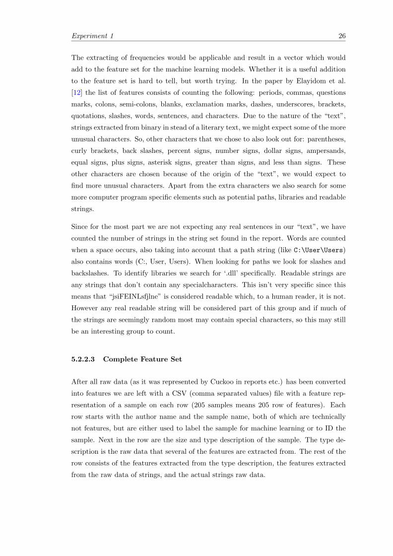
Experiment 1 26

The extracting of frequencies would be applicable and result in a vector which would

add to the feature set for the machine learning models. Whether it is a useful addition

to the feature set is hard to tell, but worth trying. In the paper by Elayidom et al.

[12] the list of features consists of counting the following: periods, commas, questions

marks, colons, semi-colons, blanks, exclamation marks, dashes, underscores, brackets,

quotations, slashes, words, sentences, and characters. Due to the nature of the “text”,

strings extracted from binary in stead of a literary text, we might expect some of the more

unusual characters. So, other characters that we chose to also look out for: parentheses,

curly brackets, back slashes, percent signs, number signs, dollar signs, ampersands,

equal signs, plus signs, asterisk signs, greater than signs, and less than signs. These

other characters are chosen because of the origin of the “text”, we would expect to

find more unusual characters. Apart from the extra characters we also search for some

more computer program specific elements such as potential paths, libraries and readable

strings.

Since for the most part we are not expecting any real sentences in our “text”, we have

counted the number of strings in the string set found in the report. Words are counted

when a space occurs, also taking into account that a path string (like C:\User\Users)

also contains words (C:, User, Users). When looking for paths we look for slashes and

backslashes. To identify libraries we search for ‘.dll’ specifically. Readable strings are

any strings that don’t contain any specialcharacters. This isn’t very specific since this

means that “jsiFEINLsfjlne” is considered readable which, to a human reader, it is not.

However any real readable string will be considered part of this group and if much of

the strings are seemingly random most may contain special characters, so this may still

be an interesting group to count.

5.2.2.3 Complete Feature Set

After all raw data (as it was represented by Cuckoo in reports etc.) has been converted

into features we are left with a CSV (comma separated values) file with a feature rep-

resentation of a sample on each row (205 samples means 205 row of features). Each

row starts with the author name and the sample name, both of which are technically

not features, but are either used to label the sample for machine learning or to ID the

sample. Next in the row are the size and type description of the sample. The type de-

scription is the raw data that several of the features are extracted from. The rest of the

row consists of the features extracted from the type description, the features extracted

from the raw data of strings, and the actual strings raw data.

Experiment 1 27

5.2.3 Machine Learning

After the feature extraction we have a data set of the samples each represented as a

number of features extracted from it and the name of the corresponding author. The

problem that we want to solve with machine learning is finding a mapping from feature

to author name, so future samples that we want to attribute can be mapped to an author

name. To model this problem we first need to find a fitting machine learning model.

The feature set we have to work with consists of numeric representations (counts) of

some of Cuckoo’s findings and the set of strings that Cuckoo extracts from the sample.

Since most machine learning models take only numeric input, the textual input (the

strings) will be classified differently. For the textual feature the Bag of Words model

one of the few models suitable. The Bag of Words, as the name indicates, is specifically

meant for classification based on a set of words. For the numeric features there are a

number of machine learning models to choose from.

CSVBag ofWords

String Features

RandomForestTesting

RandomForest

Training

ML ModelTraining

ML ModelTesting

Numeric Features

Numeric Features

AverageAccuracies

Figure 5.3: Machine Learning schematic

FINDING THE RIGHT MODELS

There are many different machine learning (ML) models and they can be classified

according to different traits [21, 22]. In choosing a ML model these different traits are

compared to find a model best suited for the problem to solve.

The first way of categorizing ML models is according to their learning methods: super-

vised learning, unsupervised learning, and reinforcement learning. Supervised learning

methods predict outcomes given a set of predictors, it maps inputs to output. Unsuper-

vised learning methods cluster the samples in groups. Reinforcement learning methods

are trained to make certain decisions and trains itself continuously through trial and

error. Reinforcement learning is often used in robotics where a decision is made based

on the input from the sensors at each step. Supervised learning appears to be the most

Experiment 1 28

suitable in this case since our problem consists of a set of features accompanied by la-

bels (the author name), and there is simply need for a mapping from input (features)

to output (labels).

Once having chosen for supervised learning, a distinction can be made between a clas-

sification or a regression model. The basic difference is that a classification model maps

an input to a discrete output (or a label) and a regression model maps input to a con-

tinuous output (a quantity). For this experiment a classification model seems the most

appropriate, with the author names as labels.

Other criteria taken into account are whether or not the model is linear and whether it

is a two- or multi-class classification algorithm. Classification algorithms that are linear

expect that the different classes can be divided by a straight line. However if the data

is nonlinear in trend, a linear model would produce more errors than necessary. As for

the two- or multi-class classification: the classes our samples can be classified in are the

author names, which is a set of known authors larger than two, making any two-class

classification algorithms less suitable.

Based on the previous discussion the following models are selected to build and test for

accuracy with our data set:

• K-Nearest Neighbors

• Decision Tree

• Random Forest

• Neural Network

For each of these models a short description and short discussion of the implementation

is given. For the full implementations see Appendix B.

Each model is given the features training set, the labels training set, and the features

testing set. With the training sets the model is trained and once trained it can predict

the associating labels for the testing set. These predictions can come simply in the form

of a label, but also come in the form of a set of floats for each label that indicates the

models confidence in that label being the right one for the features.

MODEL EVALUATION

In contrast to the real machine learning models, we have also created the simple random

classifier which does nothing other than choose a random label as output for each test

sample. The accuracy of this model is added to give a better relative understanding of

the accuracy values.

Experiment 1 29

To compare the different models we will compare their accuracies. Each model is built

(or trained) and tested twenty times and the accuracies of each are combined together

into one average accuracy of the model. For the above models only the numerical features

are used. The textual feature will be used separately for classification (Bag of Words).

The data set we have after features extraction is split into features and labels, to be the

input and output of the models respectively. The features and labels are then split into

a training set and a testing set, in a 80%-20% proportion. This splitting into training

and testing makes sure that each class is equally distributed over these sets according

to the given 80%-20% proportion.

During the accuracy calculations of each of the models, calculations were also made for

each author. This might highlight if some authors are easier to classify than others.

The textual features that were split off from the rest of the feature set earlier, are

used to train and test the Bag of Words model. With the textual features the Bag of

Words model is trained and tested. The splitting, first into features and labels, and then

into training and testing sets, happens in the same way that it does for the numerical

features. The Bag of Words model will also return its predictions for the features in the

testing set. By combining the predictions of both models, whatever model is used on the

numerical features and the Bag of Words, the combined model may be more accurate

because it uses more (types of) features (as shown in figure 5.3).

5.2.3.1 K-Nearest Neighbors

The k-nearest neighbors classification algorithm uses “lazy learning”. The training set

is not actually used to build the model, it is used as a reference whenever a new sample

is to be classified. It will try to find the k closest training examples to determine the

correct class.

The python sklearn library1 has a KNeighborsClassifier with which the k-nearest neigh-

bors algorithm2 can be implemented.The key settings for the algorithm were the number

of neighbors (set to 3) and the weight function (set to distance). These settings were

based on several experiments where the accuracy was used to determine the algorithms

settings. As part of these same experiments the algorithm for computing the nearest

neighbors was set to the kd tree algorithm.

1http://scikit-learn.org/stable/2Please refer to the appendix B for the implementation and algorithm settings.

Experiment 1 30

5.2.3.2 Decision Tree

Decision tree classification uses a tree-like graph modeling the decisions made to classify

input. Each node represents an internal decision, which is implemented by a function

returning a discrete value that is used to decide which branch to follow to the next node

or leaf. Leaves are found at the ends of the tree, they contain the labels that the tree

can return as output.

In python, the sklearn library has a DecisionTreeClassifier which makes it easier to build

a decision tree. The DecisionTreeClassifier allows for the setting of several variables,

including what function to use for measuring the quality of a split, how many features

to consider for a split, and the maximum depth of the tree. After testing a range of

depth settings on the accuracy, the maximum depth of the tree was set to 25. This is

the only setting we changed.

5.2.3.3 Random Forest

A random forest classifier is a model composed of a number of decision trees. Each of

the trees returns the label it has classified a sample in and the random forest returns

the label which appears most often among those decision trees. By combining multiple

decision trees into a random forest would boost the performance of the model.

Building this model with python, the sklearn library3 offers a RandomForestClassifier

that allows you to decide on a number of settings like the number of trees used or the

depth the trees are allowed to achieve. Some of the more influential settings are dis-

cussed. Based on experiments to determine the accuracy only one setting was changed:

the number of trees in the forest.

The setting of the number of trees in the random forest is by default 10 trees. The

experiments indicated that the accuracy of the model no longer improved after a certain

number of trees and may even decrease slightly. The experiments determined that the

trade-off between accuracy and compute performance was optimal between 25 to 50

trees. A setting of 35 trees was chosen.

5.2.3.4 Neural Network

The idea of the neural network model is a very simplified version of the neural network

of the brain. It constitutes a number of nodes or neurons, of which the output of each is

3http://scikit-learn.org/stable/

Experiment 1 31

calculated using a non-linear function on the sum of its inputs. Usually these nodes are

organized in layers, where each layer may have a different function that the nodes use

to convert input to output. Data travels from the first (input) layer, through the layers

(maybe even several times), to the last (output) layer.

To build a neural network in python we made use of the MLPClassifier offered by the

sklearn library. MLP stands for multi-layer perceptron. MLP creates an input layer,

an output layer and a number of hidden layers in between. The input layer represents

the input features and has as many nodes. The output layer converts its inputs into

output values. The MLPClassifier has many possible settings, which usually indicates

a flexible model, but also means that there is probably need for much trial and error.

There are many settings and not all of them will be discussed, only a couple of them

that are interesting or made a significant difference in accuracy.

The first two steps in configuring the neural network requires the setting of the number

of nodes per layer and the number of layers. Computational complexity increases rapidly

with the increase of both layer and nodes. Accuracy experiments led to the choice of

a single layer with 250 nodes. It is possible that a higher accuracy is obtainable but

due to time and scope limitations, this is the setting that was chosen for the neural

network model. The remaining two important settings are the threshold function and

the optimizer function. Using the previous experiments two threshold function settings

were evaluated: the tanh and the logistics. Final choice was the logistics function.

Similarly, the choice for the optimizer was the adam which is a stochastic gradient-

based optimizer.

5.2.3.5 Modeling the String Features

As explained before, the string features cannot be inserted into just any model, as most

models only accept numerical values. One of the popular methods to convert words into

vectors is the Bag of Words model. After this conversion a random forest is used to

classify.

The bag of words model is fairly simple and can achieve great results in language mod-

eling and document classification. Basically the bag of words model represents a set of

words of which only the multiplicity is stored, the original word order is insignificant.

There are a couple of measures that can help decrease the size of the vocabulary, such

as ignoring cases, taking only the stem of the words (like “walk” from “walking”) and

removing stop words like “the” and “it” and so on. In this way, by counting the occur-

rences or calculating the frequencies of the words, a set of words can be turned into a set

Experiment 1 32

of numerical features. After conversion the features can be used in any other machine

learning model like for example a random forest.

The workings of a random forest have been explained earlier. The string features are

changed into numerical features by the bag of words, which are then fed into the random

forest which returns probabilities for each sample that it should be classified under a

certain label.

5.3 Results

First the results of each of the tested machine learning models will be presented. Followed

by a more detailed look of the accuracies, examining of the different authors.

5.3.1 Model Comparison

The statistics of the models can help to compare the models, based on accuracy and the

confidences of the models. The confidences shown here are the average confidences of the

model in the classification that it returned, making a distinction between classification

that turned out to be correct and those that turned out to be incorrect. These statistics

are presented in Table 5.1. To further illustrate the results presented in Table 5.1, the

average confidence for the Random Forest (RF) model when finding the CORRECT

author for a specific sample was 0,62 (second to the right column). The confidence in an

author INCORRECTLY recognized by the Random Forest model was on average 0,35

(rightmost column). A good model is characterized by high accuracy, high confidence

in correct class choices and low confidence in wrong class choices.

The names of the models are shortened: K-Nearest Neighbors (KNN), Decision Trees

(DT), Random Forest (RF), and Neural Network (NN).

The first observation that can be made is that every real machine learning model per-

formed better than the random selection algorithm. Of these real machine learning

models, the Random Forest achieves the highest accuracy. The Decision Tree performs

second best in accuracy. However the confidence of the decision tree is high even when

it wrongly classifies a sample. All the other models have a much lower confidence when

wrongly classifying compared to the confidence when correctly classifying.

The accuracies of the complete model, with both the Random Forest and the Bag of

Words, are presented in table 5.2. Unfortunately these accuracies were calculated with

Experiment 1 33

ML Model Accuracy Avg Conf Correct Class Avg Conf Wrong Class

5Samplesperauthor

Random 2,47% - -KNN 43,24% 0,91 0,64DT 50,68% 0,99 0,99RF 57,02% 0,62 0,35NN 11,08% 0,79 0,06

10Samplesperauthor

Random 2,91% - -KNN 55,96% 0,92 0,67DT 65,37% 1,0 0,99RF 72,57% 0,71 0,35NN 9,49% 0,56 0,08

Table 5.1: Average accuracies and confidences

a random forest that was not optimally set up and thus has a lower accuracy than the

one tested above4.

5 Samples per author 10 Samples per author

Nr of testing samples 41 72

Correctly classified 48,78% 77,78%

Incorrectly classified 51,22% 22,22%

Avg confidence correct classification 0,41 0,49

Avg confidence incorrect classification 0,28 0,35

Table 5.2: Accuracies of Random Forest with Bag of Words

From the random forest some other interesting information could be ascertained. After

fitting and building a random forest with the features, the importance of these features

can be extrapolated from the random forest. These would indicate which features were

most helpful in the classification process. When a decision tree makes a split, it tries

to maximize distinciton so each branch eventually leads to maximum purity (1 possible

author in this case). A feature’s importance is the average increase in purity across all

the trees in the random forest. The importances are presented in graph 5.4. A larger

version can be found in Appendix C.

From the importance scores it appears that the features that are the most important

are the size and type features, followed by the string frequencies and finally the counts

of DLLs and paths etc.

5.3.2 Analysis of Authors

To portray the accuracies depending on author we present a table and two graphs, both

of which can be found in Appendix D. The table (Table D.1) shows the accuracies per

4Experiments could not be repeated because I no longer had access to the sample database.

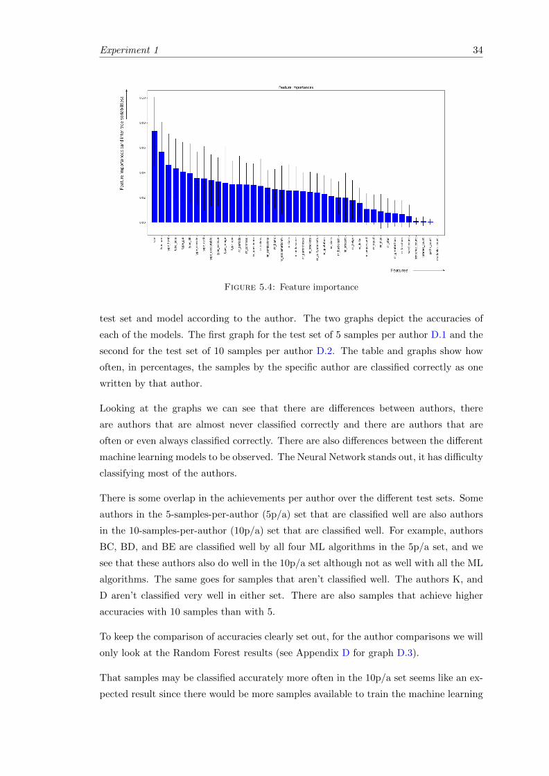
Experiment 1 34

Figure 5.4: Feature importance

test set and model according to the author. The two graphs depict the accuracies of

each of the models. The first graph for the test set of 5 samples per author D.1 and the

second for the test set of 10 samples per author D.2. The table and graphs show how

often, in percentages, the samples by the specific author are classified correctly as one

written by that author.

Looking at the graphs we can see that there are differences between authors, there

are authors that are almost never classified correctly and there are authors that are

often or even always classified correctly. There are also differences between the different

machine learning models to be observed. The Neural Network stands out, it has difficulty

classifying most of the authors.

There is some overlap in the achievements per author over the different test sets. Some

authors in the 5-samples-per-author (5p/a) set that are classified well are also authors

in the 10-samples-per-author (10p/a) set that are classified well. For example, authors

BC, BD, and BE are classified well by all four ML algorithms in the 5p/a set, and we

see that these authors also do well in the 10p/a set although not as well with all the ML

algorithms. The same goes for samples that aren’t classified well. The authors K, and

D aren’t classified very well in either set. There are also samples that achieve higher

accuracies with 10 samples than with 5.

To keep the comparison of accuracies clearly set out, for the author comparisons we will

only look at the Random Forest results (see Appendix D for graph D.3).

That samples may be classified accurately more often in the 10p/a set seems like an ex-

pected result since there would be more samples available to train the machine learning

Experiment 1 35

model. Also the 10p/a set has a slightly smaller pool of different authors, which could

also account for an increase in accuracy. The significant decrease in accurate classifi-

cation is less expected, and only applies for a small number of authors. Perhaps these

authors don’t have a standard process in creating their malware, or perhaps (also) use

code that is not their own. Looking more closely at the features we can see that the

samples of most authors are all of the same type. Most samples are of the type “PE32

executable (GUI)”, so samples that are of a different type are likely to What stands out

in the samples belonging to author BE is that all of the character-count features 0 or

almost 0. None of the other samples have this which is likely to be the reason the author

BE is recognized so well.

Chapter 6

Experiment 2: Obfuscation and

information loss in Cuckoo

reports

In this experiment the goal is to gain better insight into what different types of obfus-

cation can mean for feature extraction during malware analysis. In other words, what

remains of the features of the malware after it has been obfuscated.

6.1 Sample Selection

Samples of real malware with knowledge on the author of the malware are no longer

accessible to us. Therefore we will collect and examine different types of “normal”

non-malware samples.

A number of samples, see Appendix E, are collected from the 2017 Google Code Jam1.

These samples are rather small and only do some calculations. These may not offer

much in the sense of dynamic observation, but can be related back to an author. A total

of 45 samples, 9 authors with each 5 samples, are selected. The five samples chosen

of each author are solutions to the same five challenges. The authors and samples are

chosen to all have been written in the same programming language, in this case C++.

1https://www.go-hero.net/jam/17

36

Experiment 2 37

6.2 Sample Preparation

The selected samples are available as source code and will first need to be compiled.

Since it concerns C++ code we use Microft Visual Studio C++ 2017 (version 15.6.3)

for the compiling.

For the preparation of the obfuscated samples a number of (free) obfuscation tools are

chosen. Packers are the most popular type of obfuscation tool and there are many

different ones available online, a number of which for free (or trial). These packers

range from very simple ones to ones that have extra options such as encryption and

anti-analysis measures.

Runtime encryption tools will function in more or less the same way as runtime packers

(as discussed in section 2.2.1), with the original executable obscured and inserted in

a type of container accompanied by a stub that allows the original executable to be

extracted at runtime. The only difference is the method of obscuring the executable,

in which even two packers can differ (different packing algorithms). The few runtime

encryption tools that can be found are outdated or can not be used on our system. For

these reasons and the fact that certain packers incorporate encryption, we will focus

mainly on packer tools and not test any specific cryptor tools.

During our search for obfuscation tools we also encountered a tool called Stunnix, which

claims to be a general obfuscator but which is applied to the source code and we will

therefore refer to as a source code obfuscator. This tool is included in the set of obfus-

cation tools used for this experiment, for comparison.

The packers are applied on the executable itself. The Stunnix tool is applied to the

C++ code before compilation. The list of obfuscation tools:

• UPX (packer)

• Themida (packer)

• Stunnix (general obfuscator)

After obfuscation the samples are still executables and can still be executed. The re-

sulting sample set with which this experiment will be run are summarized in table 6.1.

Obfuscation and several techniques have already been covered in Chapter 2 on Malware.

Here you will find a short summary of the techniques and tools used for this experiment.

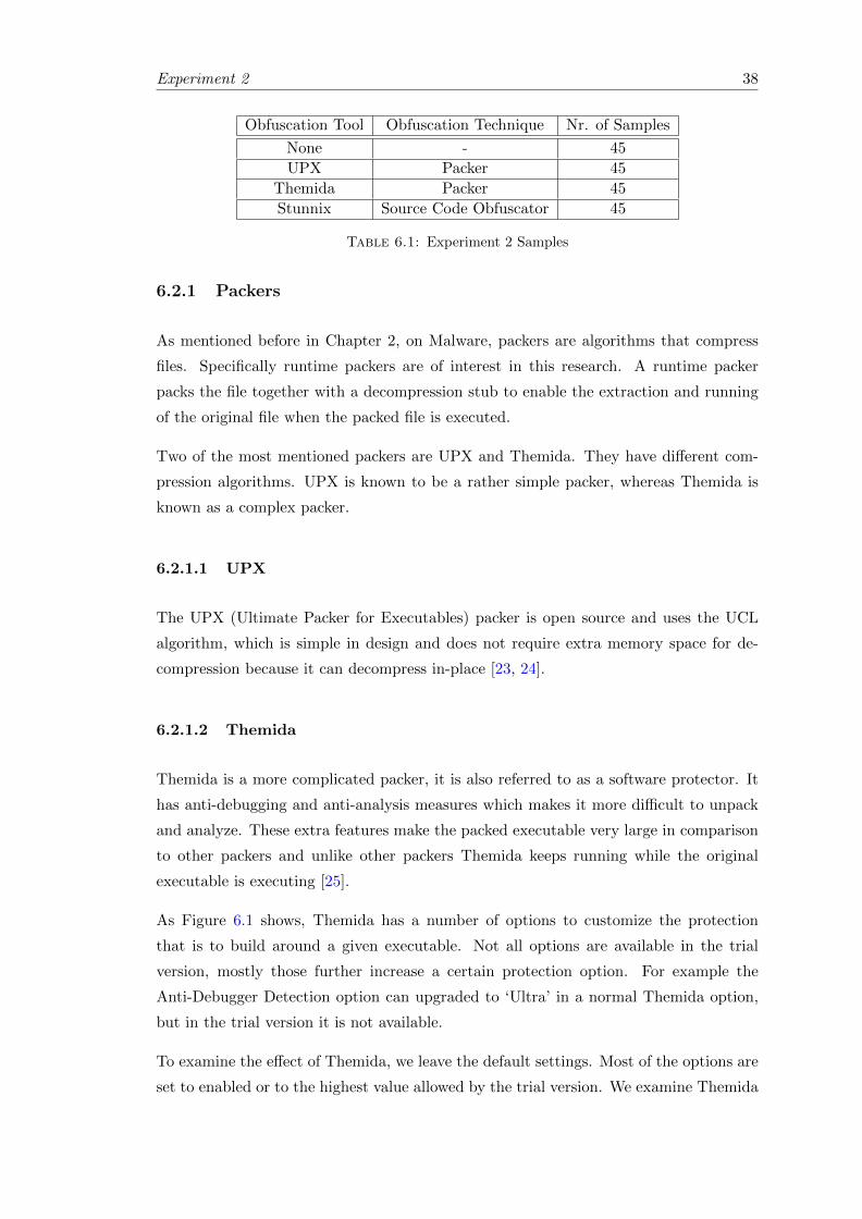
Experiment 2 38

Obfuscation Tool Obfuscation Technique Nr. of Samples

None - 45

UPX Packer 45

Themida Packer 45

Stunnix Source Code Obfuscator 45

Table 6.1: Experiment 2 Samples

6.2.1 Packers

As mentioned before in Chapter 2, on Malware, packers are algorithms that compress

files. Specifically runtime packers are of interest in this research. A runtime packer

packs the file together with a decompression stub to enable the extraction and running

of the original file when the packed file is executed.

Two of the most mentioned packers are UPX and Themida. They have different com-

pression algorithms. UPX is known to be a rather simple packer, whereas Themida is

known as a complex packer.

6.2.1.1 UPX

The UPX (Ultimate Packer for Executables) packer is open source and uses the UCL

algorithm, which is simple in design and does not require extra memory space for de-

compression because it can decompress in-place [23, 24].

6.2.1.2 Themida

Themida is a more complicated packer, it is also referred to as a software protector. It

has anti-debugging and anti-analysis measures which makes it more difficult to unpack

and analyze. These extra features make the packed executable very large in comparison

to other packers and unlike other packers Themida keeps running while the original

executable is executing [25].

As Figure 6.1 shows, Themida has a number of options to customize the protection

that is to build around a given executable. Not all options are available in the trial

version, mostly those further increase a certain protection option. For example the

Anti-Debugger Detection option can upgraded to ‘Ultra’ in a normal Themida option,

but in the trial version it is not available.

To examine the effect of Themida, we leave the default settings. Most of the options are

set to enabled or to the highest value allowed by the trial version. We examine Themida

Experiment 2 39

Figure 6.1: Themida window, showing the protection options

for its complexity, which is in part due to these extra protection options. So we want

to take these options, that an attacker can easily just enable, into account when testing

Themida.

6.2.2 Source Code Obfuscator

The obfuscation tool named Stunnix, which obfuscates the source code directly, takes

obfuscation measures like: replacing symbol names, changing numeric constants and

characters in strings to meaningless or more difficult to read variants, removing or ob-

fuscating comments, and renaming files and directories to make them meaningless. Since

Stunnix is run on the source code, it has no effect on anything that happens to the code

afterwards like compilation and obfuscation.

6.3 Experiment Architecture

The goal of this experiment is to determine what the effect is of obfuscation on the

analysis and its findings of executables.

Experiment 2 40

Each of the samples, whether obfuscated or not, is run in Cuckoo Sandbox resulting in

a report of extracted information. The reports of each of the non-obfuscated samples

can be compared to the reports of the obfuscated versions of that sample.

Any data in the Cuckoo reports that is missing or altered after obfuscation is of interest,

because these seem to be affected by the obfuscation tool used. Elements of the report

that will be analyzed for consequences of the obfuscation include: the size of the sample,

the imported libraries, the type, the strings that can be extracted, and whether Cuckoo

recognizes that the sample has been obfuscated and with what.

6.3.1 Sample Submission

The samples are submitted to Cuckoo Sandbox with a chosen timeout of 120 seconds

(basically the duration of the analysis), due to the fact that these samples are very small

calculation programs and will not need much time to run.

6.3.2 Report Analysis

Part of the analysis of the reports resulting from the Cuckoo Sandbox analysis will be a

manual examination of 10 randomly selected samples, meaning that 10 non-obfuscated

samples are manually compared to each of their obfuscated counterparts (the UPX,

Themida and Stunnix versions). In each of the different sections of a report of an

obfuscated sample we look for differences compared to the same section the report of

the non-obfuscated version.

Another form of analysis is a type of point tallying. To compare the amount of infor-

mation lost after obfuscation, the data will be quantified with a points system: each

feature found in the Cuckoo report is worth 1 point, e.g. the non obfuscated version

of the sample has the maximum amount of points. For each feature that is missing

or altered in the obfuscated versions, points are deducted from the maximum amount.

Since each feature is worth 1 point, every missing feature costs 1 point. The cost of a

feature whose content is altered is 1/2 points.

6.4 Results

On examination of Cuckoo analysis reports, which are in JSON format, the sections

found in each are:

Experiment 2 41

info contains info about the analysis itself: when it started, how long it lasted, its ID

number, on what machine it was run, etc.

signatures indicates whether any signature matches are found in the sample. One of

these is whether the sample uses the known packer UPX

target identifies the sample submitted for analysis, such as its name, size and hashes

network lists the type of network connections made during the analysis period

static contains any information extracted by static analysis, in the case of Windows

executables mostly PE format information including a detailed list of imports

behavior contains information extracted with dynamic analysis, such as processes run

(including API calls) and a process tree

debug section in which Cuckoo writes its logs and other debug statements made during

the analysis

strings lists all strings found in the analyzed sample

metadata doesn’t contain much, but lists any other output created during the analysis

such as a pcap file (based on my observation)

A shortened example of a report is shown in Appendix F.

6.4.1 Manual Reports Analysis

Of the sections present in the cuckoo report, several do not actually portray information

pertaining to the sample itself but rather status on how Cuckoo was running the sample.

This type of information is not suitable for this experiment. The sections that will be

investigated are: signatures, target, static, behavior, and strings. The network section

is exempt from analysis as well since the analyzed samples (by design) do not create any

network traffic and therefore each network section contains no relevant information.

The signatures, target, static and strings sections seem to contain information only

obtained by means of static analysis. The behavior section contains information only

obtained by dynamic means. In analyzing the reports for differences between obfus-

cated and non-obfuscated versions, a distinction between these two types of features

will maintained.

In the set of static features there are variations to be found in the reports of obfuscated

samples in comparison to the static results of the non-obfuscated samples. Only the

Experiment 2 42

samples obfuscated with Stunnix show little change because the tool applies obfusca-

tion on the code not the compiled executable, meaning that any information available

after/from compilation stays as it is.

The dynamic features seem less affected by the obfuscation tools. UPX and Stunnix

do not seem to have any affect at all, Themida however adds a surprising amount of

dynamic behavior that Cuckoo reports on.

The only obfuscation tool that Cuckoo seems to recognize by actually naming it is UPX,

in the type description Cuckoo specifically states ‘UPX compressed’. The other tools are

not mentioned specifically, possibly because it may be difficult to distinguish between

different tools.

For each of the tools used for obfuscation we will list the observed differences in the

features extracted in comparison to the same files without obfuscation, including a couple

of examples. In short table format the changes affected by the obfuscation tools on the

static features can be found in table 6.2, and the changes on the dynamic features can

be found in table 6.3.

A ‘-’ means that some information has been obfuscated, a ‘+’ means that more details

are given than in the non obfuscated version, and a ‘<>’ means that a change in value

was observed, but that it can’t be quantified as more or less just different. If none of

these symbols are used, the data was unchanged in comparison to the non obfuscated

sample.

Size Type Compile Time DLL DLL Imphash PEiD StringsPath Stamp Count Imports Signatures

UPX - + - <> <> -

Themida + - - - <> - -

Stunnix <>

Table 6.2: Observed changes to static features after obfuscation

Registry Keys Read File Opened DLL Loaded Api Stats Processes

UPX

Themida + + + + +

Stunnix

Table 6.3: Observed changes to dynamic features after obfuscation

For each of the tools used for obfuscation we will list the observed differences in the

features extracted in comparison to the same files without obfuscation, including a couple

of examples.

Experiment 2 43

Differences UPX:

• Static

– Decreased file size

– All the signatures are now indicative of a packer and the UPX packer in

particular

– The pdb path is missing

– Most of the imports are missing

– There are a smaller number of PE sections, the majority of identified sections

have names like “UPX0” and “UPX1”

– The set of strings is much smaller and contains different strings

• Dynamic

– N.a.

Differences Themida:

• Static

– Increased file size

– Increases significantly the number of signatures activated, mostly packer type

and or anti-debugger or -forensic related

– The pdb path is no longer known

– Most of the imports are missing

– Different imphash (the imphashes of the Themida samples are all the same)

– There are fewer sections, and these sections seem different

– More, but less readable, strings found

• Dynamic

– More “generic” information such as files opened, registry keys read, dlls

loaded, etc.

– More api stats (which lists the used api’s followed by the number of times

used)

– More calls made by the process, including many ‘timeGetTime’ synchroniza-

tion calls

Experiment 2 44

Differences Stunnix:

• Static

– The .text, .rdata, and .reloc PE sections have different entropy and virtual

sizes

– Some minor changes and additions in the set of strings, often including some

“Replacement For” additions

• Dynamic

– N.a.

6.4.2 Info Points

Next we present the calculated score of each sample. An overview of the information

loss as a result of obfuscation, by the tallying of present information, is given in a table

found in Appendix G. What can be observed from the table is that Stunnix has the

smallest impact on the amount of information that Cuckoo can find, with an average

of 5 points more or less. The UPX packer roughly halves the number of points. And

the Themida samples all seem to have roughly the same number of points, on average

2385 points, which is more than double the amount of points the samples have without

obfuscation.

Some points are missing because the samples were missing. UPX had trouble packing

one of the samples, acmonster 17 2-A, which was unpackable according to UPX. Stunnix

had a similar problem with four samples, for which it could not create an obfuscated

version for a non-specific reason (possibly due to the simple nature of the samples).

Chapter 7

Evaluation & Discussion

Here we evaluate the results of both experiments separately, followed by a discussion on

the combined results.

7.1 Experiment 1

At the end of experiment 1 two sets of results were presented, the differences in author

and the comparison of the machine learning models.

Looking first at the machine learning model comparisons, the results are shown here

again in Table 7.1 which represents the two test sets with samples. The first consisting

of 37 different authors each with 5 samples, and the second with 34 different authors

each with 10 samples.

ML Model Accuracy Avg Conf Correct Class Avg Conf Wrong Class

5Samplesperauthor

Random 2,47% - -KNN 43,24% 0,91 0,64DT 50,68% 0,99 0,99RF 57,02% 0,62 0,35NN 11,08% 0,79 0,06

10Samplesperauthor

Random 2,91% - -KNN 55,96% 0,92 0,67DT 65,37% 1,0 0,99RF 72,57% 0,71 0,35NN 9,49% 0,56 0,08

Table 7.1: Average accuracies and confidences

All of the machine learning models perform better than the random model, but certain

models clearly perform better than others. The Neural Network is not at all reliable,

45

Evaluation & Discussion 46

with accuracies of about 9,5% and 11%. The Random Forest appears to be the most

accurate model, followed by the Decision Tree.

We can also observe that the accuracies are significantly higher when we use 10 samples

per author in stead of 5 samples per author. This is likely due to 1) there being more

samples per author for the model to learn from in the 10-samples-per-author test case

and 2) there being less different authors to model in the 10-samples-per-author test

case. As we can see, even the Random model has an increased accuracy in the case of 10

samples per author compared to the 5 samples per author case. However it is unlikely

to be the reason for the complete 15,55% difference that we see with the Random Forest

classifier. Only in the case of Neural Networks this does not seem to apply. Perhaps our

problem has not been or could not be modeled properly by our Neural Network.

Another aspect to consider are the confidences of the models. With the Decision Tree

model the confidences in classification are always about 100% (1,0). The Random Forest

has a much lower confidence when classifying samples incorrectly as opposed to when

classifying them correctly. This difference in confidence can allow for the setting of a

threshold for example, allowing the model to classify only when its confidence in the

classification is higher than a predetermined minimum. Using a threshold means that

the model may not be able to classify certain samples because its confidence is not high

enough, but will most likely result in less wrong classifications and thus help the model

be more accurate with the samples that it does classify.

5 Samples per author 10 Samples per author

Nr of testing samples 41 72

Correctly classified 48,78% 77,78%

Incorrectly classified 51,22% 22,22%

Avg confidence correct classification 0,41 0,49

Avg confidence incorrect classification 0,28 0,35

Table 7.2: Accuracies of Random Forest with Bag of Words

The results discussed up to now are the results of the different ML models based on

the numeric features. However we also had string features that were transformed into

numeric features with the use of Bag of Words after which a Random Forest was trained

and tested with these features. The confidences of this Random Forest were then aver-

aged with the confidences of the Random Forest for the initial numeric features, which

resulted in the accuracies and confidences shown in table 7.2. The Random Forest used

here did not have the optimal settings like the Random Forest in table 7.1. When recal-

culating the accuracies it must have resulted in, with the original settings and without

the strings involved, they resulted in accuracies of 10% and less. This would suggest

Evaluation & Discussion 47

that with the better Random Forest (see in table 7.1) in combination with the strings

modeling, we could expect higher accuracies.

7.1.0.1 Feature Importance

After concluding that the Random Forest model performs best in our case, the feature

importance according to the Random Forest is examined. The feature importance in

Appendix C shows which features were most important in the building of the random

forest, to make distinguishing decision forks to better classify any samples. These are,

in order: the size and type features, followed by the string frequencies and finally the

counts of DLLs and paths etc. For the type features this may seem logical, since it is

feasible that attackers might specialize in a certain type of malware. However the size

features ranking so high is unexpected. The size of a program is not only dependent on

the code and compilation method but also on any other tools used on it like packers.

Using a different packer can change the size, but the (original) program and author

would not be different. Perhaps if an author consistently used the same compiler and

obfuscation methods that the size of his/her software would always fall within a certain

range, but it does not seem logical to take this as the most reliable feature.

Another observation to be made about the feature importance is that although the string

frequencies are considered less important for the modeling than the type features, their

importance is not much lower. The more unusual characters that we chose to also count

and add to the feature set are in the same range of importance as the standard periods,

commas, question marks, etc. Only the mathematical characters, like the plus sign and

greater than sign etc, perform significantly worse.

The counting of the certain types of strings found (libraries, paths and readables) were

not useful at all, their importance is 0. The word and sentence count are of the lowest

importance higher than 0. The counting of these types do not seem like useful additions

in the case of malware attribution.

7.1.0.2 Author-specific Statistics

From the author-specific statistics, which can be found in Appendix D, it would seem

that some authors are classified more accurately than others. This prompts the question

whether this is by accident or whether it may actually mean that compiling styles and

possible specific obfuscation uses of some authors make their work more unique and

recognizable.

Evaluation & Discussion 48

Given our current methods and results it is not possible to give any definitive answer to

this question, only that it may be an interesting aspect to explore. With a larger pool of

authors differences between authors might become less pronounced probably resulting

in lower accuracies. However those authors that really do stand out would still have

high accuracies.

7.1.1 Reflection

The experiment was not without its problems. There are several aspects of the exper-

iment that we would like to reflect on, some elements of the experiment did not go as

expected.

To start with, in using virtual machines to analyze the samples, some of the samples

may not have been analyzed properly if they incorporated any anti virtual machine

techniques. We did not actually investigate if there were any such cases, but assumed

that if this affected the Cuckoo results the anomalies would result in features. Thereby

distinguishing authors that take such type of measures.

Another aspect of the experiment that did not meet our expectations was the number

of different authors that we could find. Due to the somewhat limited pool of authors

used for the experiment, no conclusions can be made on the effectiveness in real world

situations where the number of possible malware authors is bound to be much higher

and, as likely, authors that are not in the pool yet (e.g. unknown).

Other issues with the experiment are the use of static features only and having initially

used a less than optimal machine learning setup to calculate the total accuracies (Bag of

Words included). Especially since we expect that the total (averaged) accuracies would

be higher if the results of the strings’ modeling had been added. These shortcomings

were mainly due to a limited time to access the malware samples forcing some quick

decisions to be made.

Dynamic features had not been available at the time due to inexperience with Cuckoo

and not knowing that the Cuckoo agent was to be run in administrator mode for Cuckoo

to properly analyze the behavior of a sample. There were other static features that

could have been extracted from the Cuckoo reports, however at the time it was decided

to build the rest of the experiment on the couple of features that we had and expand

on the features in the future. Unfortunately we were not able to make time for this

expansion.

Finally we would like to observe that in designing the machine learning setup, we chose

to deal with the problem as a one out of many situation. Meaning that the author of a

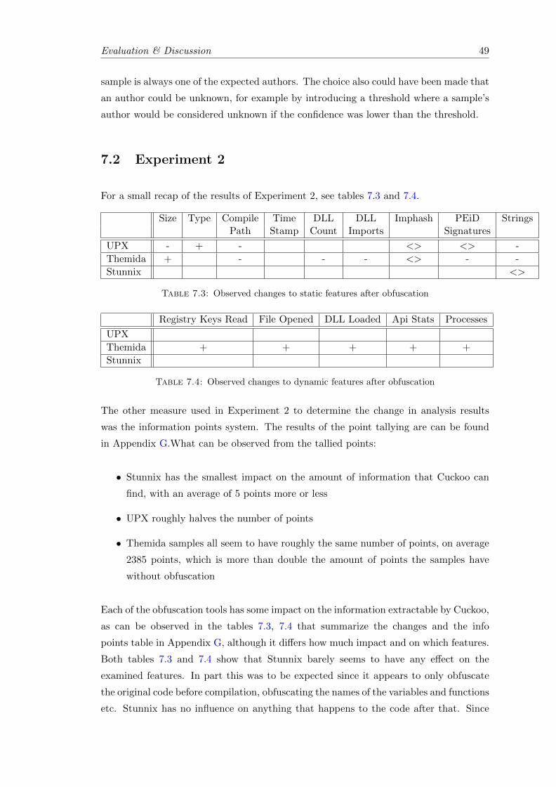
Evaluation & Discussion 49

sample is always one of the expected authors. The choice also could have been made that

an author could be unknown, for example by introducing a threshold where a sample’s

author would be considered unknown if the confidence was lower than the threshold.

7.2 Experiment 2

For a small recap of the results of Experiment 2, see tables 7.3 and 7.4.

Size Type Compile Time DLL DLL Imphash PEiD StringsPath Stamp Count Imports Signatures

UPX - + - <> <> -

Themida + - - - <> - -

Stunnix <>

Table 7.3: Observed changes to static features after obfuscation

Registry Keys Read File Opened DLL Loaded Api Stats Processes

UPX

Themida + + + + +

Stunnix

Table 7.4: Observed changes to dynamic features after obfuscation

The other measure used in Experiment 2 to determine the change in analysis results

was the information points system. The results of the point tallying are can be found

in Appendix G.What can be observed from the tallied points:

• Stunnix has the smallest impact on the amount of information that Cuckoo can

find, with an average of 5 points more or less

• UPX roughly halves the number of points

• Themida samples all seem to have roughly the same number of points, on average

2385 points, which is more than double the amount of points the samples have

without obfuscation

Each of the obfuscation tools has some impact on the information extractable by Cuckoo,

as can be observed in the tables 7.3, 7.4 that summarize the changes and the info

points table in Appendix G, although it differs how much impact and on which features.

Both tables 7.3 and 7.4 show that Stunnix barely seems to have any effect on the

examined features. In part this was to be expected since it appears to only obfuscate

the original code before compilation, obfuscating the names of the variables and functions

etc. Stunnix has no influence on anything that happens to the code after that. Since

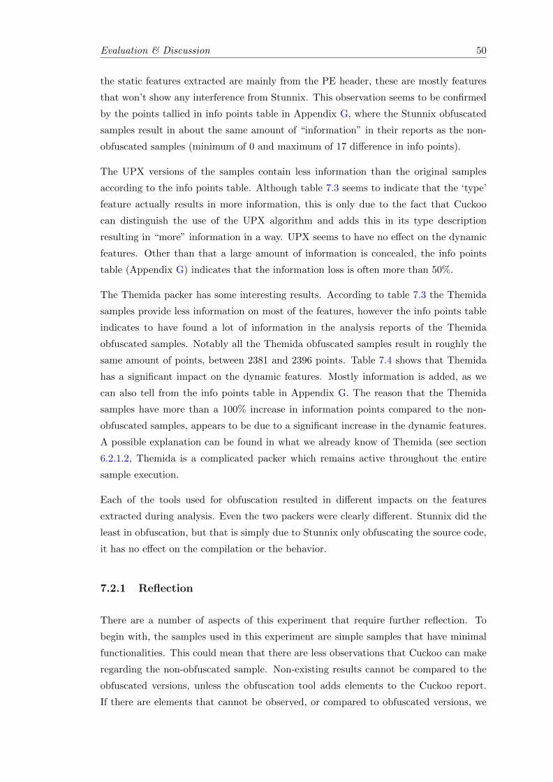
Evaluation & Discussion 50

the static features extracted are mainly from the PE header, these are mostly features

that won’t show any interference from Stunnix. This observation seems to be confirmed

by the points tallied in info points table in Appendix G, where the Stunnix obfuscated

samples result in about the same amount of “information” in their reports as the non-

obfuscated samples (minimum of 0 and maximum of 17 difference in info points).

The UPX versions of the samples contain less information than the original samples

according to the info points table. Although table 7.3 seems to indicate that the ‘type’

feature actually results in more information, this is only due to the fact that Cuckoo

can distinguish the use of the UPX algorithm and adds this in its type description

resulting in “more” information in a way. UPX seems to have no effect on the dynamic

features. Other than that a large amount of information is concealed, the info points

table (Appendix G) indicates that the information loss is often more than 50%.

The Themida packer has some interesting results. According to table 7.3 the Themida

samples provide less information on most of the features, however the info points table

indicates to have found a lot of information in the analysis reports of the Themida

obfuscated samples. Notably all the Themida obfuscated samples result in roughly the

same amount of points, between 2381 and 2396 points. Table 7.4 shows that Themida

has a significant impact on the dynamic features. Mostly information is added, as we

can also tell from the info points table in Appendix G. The reason that the Themida

samples have more than a 100% increase in information points compared to the non-

obfuscated samples, appears to be due to a significant increase in the dynamic features.

A possible explanation can be found in what we already know of Themida (see section

6.2.1.2, Themida is a complicated packer which remains active throughout the entire

sample execution.

Each of the tools used for obfuscation resulted in different impacts on the features

extracted during analysis. Even the two packers were clearly different. Stunnix did the

least in obfuscation, but that is simply due to Stunnix only obfuscating the source code,

it has no effect on the compilation or the behavior.

7.2.1 Reflection

There are a number of aspects of this experiment that require further reflection. To

begin with, the samples used in this experiment are simple samples that have minimal

functionalities. This could mean that there are less observations that Cuckoo can make

regarding the non-obfuscated sample. Non-existing results cannot be compared to the

obfuscated versions, unless the obfuscation tool adds elements to the Cuckoo report.

If there are elements that cannot be observed, or compared to obfuscated versions, we

Evaluation & Discussion 51

could be missing some effect that the obfuscation tool otherwise would have. This could

limit our understanding of the influence of the obfuscation tool.

Another observation to be made on this experiment is that the packer Themida has

several protection options when obfuscating. It can monitor for sandbox tools, enable

encryption, have a memory guard, etc. We did not try different variantions of the tool,

but only used the default settings in large part because the default settings already

involved many of these extra protection options. Still it would have been interesting to

compare the effect of Themida stripped down to compression only and Themida with

extra protection options. This would allow to determine what features are inherent of

Themida possibly allowing for the recognition of Themida.

7.3 Discussion

Even though only a few static features are used in Experiment 1, the results still seem to

indicate that there could possibly be some basis for use of such features in a classification

model. An increase in accuracy is perceptible when using more samples per author.

However we only had a small number of authors which is not representative for “real

world” situations. Also the accuracies are not high enough to use as a stand-alone

analysis, at its current level it migth be useful as an indication at most, to perhaps

narrow the scope of potential offenders.

As Experiment 2 shows the use of obfuscation tools can have a substantial effect on the

features that Cuckoo extracts statically, the same kind of features used for Experiment

1. This would indicate that these features may not be the most reliable. The results also

show that obfuscation tools have less effect on dynamic features, however some more

complex tools (like Themida) have many dynamic features of their own which can cloud

the results.

However given that the samples used in Experiment 1 are real malware samples and the

results of Experiment 1 seem to indicate that classification according to author is possible

to some degree. If we were to assume that most malware authors do not obfuscate their

malware then at least some of these static features would stay usable for classification.

The fewer authors that would use obfuscation are distinguished because of this, but

mainly from those that don’t obfuscate. On the other hand, if we were to assume that

most malware authors do obfuscate their malware then the accuracy in Experiment 1

seems rather high. Perhaps this can be explained by looking at the malware authors

as creatures of habit, using the same obfuscators. Another possibility is that malware

Evaluation & Discussion 52

authors use rather weak obfuscation, leaving some or most of the features available for

Cuckoo.

It would have been interesting if our first experiment would have included dynamic fea-

tures. Making sure the agent.py runs in administrator mode on the testing environment

would very likely have resulted in more features to use in the classification. This might

have resulted in higher classifications.

Chapter 8

Conclusion & Future Research

Based on the experiments and their results we surmise that there are both static and

dynamic features with which an author profile or fingerprint can be built, although

certain obfuscation tools may complicate this. Using these author profiles to model the

authors and determining the author of a new sample seems possible although this was

only tested on a small scale and the accuracy is not yet as high as would be necessary

for real use. More likely it would function as a way to either narrow the search or as

extra confirmation of a specific suspect.

Cuckoo Sandbox is useful as a tool for automated malware analysis. Once it is up and

running, it is rather easy to submit samples. According to the results of experiment 1 it

would seem that even a couple of features extracted with static analysis can contribute

to classification of malware according to author. Although the feature composition

used does not achieve enough reliability to be useful. The composition needs further

improvement, such as the addition of dynamically extracted features.

We have also observed that dynamic features are less likely to be affected by obfus-

cation tools and therefore may be considered as more reliable. Especially the simpler

obfuscation tools have a limited reach and only affect the static features. However more

complex tools, like those that include extra anti-analysis protection options, can affect

the dynamic features.

8.1 Future Research

Knowing what we know now, at the end of this project, there are a number of directions

for further research. These are, in order of importance:

53

Conclusion & Future Research 54

• Extending the analysis capabilities discussion of possible analysis extensions to

provide more raw data from which the features can be extracted;

• Increasing profile and model accuracy - this would cover both the feature set as

well as the role of machine learning as part of the models as this would improve

the accuracy of the results;

• Increasing the sample database based on the accuracy results it is apparent that

with the increase of the number of available samples, the accuracy of the results

increases rapidly;

• Providing deeper insights in the sample rather than just a score and confidence,

further insights on the sample will be very useful, in particular if the sample is not

conclusively attributed to a particular author.

In the following sections we will discuss these directions in more detail.

Combining all the different elements into one completely automated system would even-

tually make it a usable tool for law enforcement. Although the output should be detailed

enough that an investigator using the tool can observe what aspects of the malware stood

out and the attribution decision was based on.

8.1.1 Sample Database

There are two ways in which the number of samples can be increased. The first and

most important, considering the possible application of a malware attribution system, is

the size of the author pool. As the number of authors to distinguish between increases,

accuracy will decrease. Any malware attribution system would have to maintain a high

level of accuracy if it is to be used in “real world” situations. The accuracy is dependent

on multiple factors, including what features are used and how it is modeled. These

factors should be such that the accuracy is not significantly impacted when greatly

increasing the author pool. To determine if this is the case a large database of malware

samples (preferably real malware) of which the authors are known would be needed.

The other aspect related to the number of samples to research is the number of samples

per author that are used to train a classification model. Usually the more samples the

classification model can learn from, the better it can recognize the different classes, in

this case authors. However, in a “real world” setting it may often not be possible to

have many samples known to belong to a certain author. What is the minimum number

of samples needed of an author to be distinguishing enough?

Conclusion & Future Research 55

Another aspect of the samples that should be considered are their complexity. Are the

author and user of a sample the same person? What happens if this is not the case?

It would be interesting to make a distinction between those features that are strictly

author related and those that identify the user. Perhaps adding weights to the features

based on their strength in connection to user and author.

Furthermore, malware can be written by multiple people. In this case the team could be

seen as a single identity if it is likely that the team composition does not vary. Or, since

it is likely that the team members would work in a modular fashion, each creating a

certain part, the sample can be analyzed as a combination of parts where each part does

not have to have the same author. This would also be an intriguing aspect to research

and probably relevant to the malware-as-a-service market.

8.1.2 Tool Environment

In Chapter 3, Related Work, we discussed several papers that we considered of interest

for our own research into automated malware attribution. The papers discuss differ-

ent aspects of (malicious) software which we considered as potentially aiding in author

identification. Some of these aspects are incorporated in Cuckoo Sandbox, but there is

(significant) room for improvement. Compiler provenance, recognizing which compiler

was used to compile the sample, will be a good addition. It adds to attribution, since it

is a decision made by the person who compiles the malware. Note that this could also

be indicative of the user instead of the author if these are not the same person.

Future research could also look at an addition of obfuscation tool recognition to Cuckoo

Sandbox. So far Cuckoo can determine whether a sample has been packed, but cannot

always resolve which packer tool was used. We have seen Cuckoo recognize UPX, but

not Themida. Since UPX is one of the simplest packers, it is likely that there are

more packers Cuckoo does not recognize. Since new packers or new versions surface

quite often, signature based recognition would have its limitations. However if the most

commonly used packers can be recognized, this would be a good addition to Cuckoo.

This would also allow for Cuckoo to try to unpack the sample based on the packer it

has estimated was used, potentially revealing more information.

8.1.3 Machine Learning

This research has only used static features for the modeling of the authors. However,

since obfuscation is less likely to affect the dynamic features, it would be interesting

to determine whether dynamic features (greatly) increase the accuracy as we would

Conclusion & Future Research 56

expect. Also, when making a distinction between user and author, the dynamic features

are more likely to reflect the style of the author, while the static features might indicate

the influence of the user.

Furthermore, the models could potentially be improved on in several aspects. There may

be machine learning models that could better model the attribution problem. As we

saw with the Neural Network model, it did not achieve high accuracies in this research

most likely due to limited experience and available time with this complex model.

Considering that the database of “known” samples is likely to be limited and possibly

not contain the author of an “unknown” sample, it could be useful to apply a threshold

to the model output. If the model’s confidence in a certain author is lower than this

threshold, the author of the sample may be unknown and will need manual analysis by

an investigator.

Another aspect that could potentially be improved on is to allow the model to keep

learning (like reinforcement learning), so it learns from new samples. Either new samples

can indicate a new author or reinforce the “profile” of an existing author already in the

database. However, the accuracy of the model would have to be high enough to not

accidentally muddle the profiles instead of extending them.

Also, if taken into account that a sample may have contribution from multiple people,

the model might return the top 5 authors, instead of only the top 1, including the

confidence the model has in each of these authors. If the model for instance were to

identify two authors both with high confidences, this might indicate that both were

involved with the creation of the malware sample.

Appendix A

Simple Encoding Schemes

Some simple encoding schemes are: Base64, XOR and ROT13.

A.1 Base64

Base64 encoding represents the input in ASCII string format. Its encoding alphabet

consists of 64 characters which are A-Z, a-z, 0-9, + and /. Figure A.1 shows how Base64

encoding works. The equal sign (=) is used as padding. This padding character is what

can make Base64 encoded text fairly easy to recognize. Because the order in which the

64 characters of the encoding alphabet are placed matters for the encoding, it is easy to

customize it. Just by moving for instance the character a to the front of the alphabet,

the encoding is changed and will create a different output.

Figure A.1: Base64 encoding example of ATT, part of ATTAK AT DAWN

A.2 XOR

The XOR cipher is a rather simple cipher. It applies the XOR (exclusive disjunction)

operator to the bits of each character with the bits of a given key. The process of

decrypting is exactly the same as that of encrypting, and so you need the key again to

57

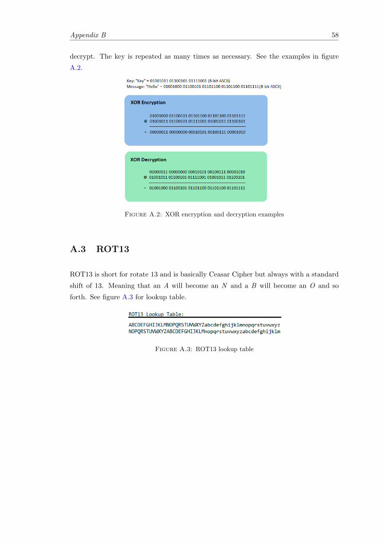
Appendix B 58

decrypt. The key is repeated as many times as necessary. See the examples in figure

A.2.

Figure A.2: XOR encryption and decryption examples

A.3 ROT13

ROT13 is short for rotate 13 and is basically Ceasar Cipher but always with a standard

shift of 13. Meaning that an A will become an N and a B will become an O and so

forth. See figure A.3 for lookup table.

Figure A.3: ROT13 lookup table

Appendix B

Classifier Implementations

Here you can find the precise implementation of each of the classification algorithms

used in Experiment 1.

For each of these implementations the data set, containing the features and labels, was

first split into features (X) and labels(y) and then again into a training (X train and

y train) and a testing set (X test and y test). The X train and y train are needed to

build the model, it allows the model to find a mapping from features to labels. The X test

lets the model predict which labels should be attributed to these features according to

its mapping. With the predict proba method the model gives its calculated probabilities

that a certain label corresponds with the features, for each possible label. The label that

has the highest probability (or confidence) is the one that the models predicts.

B.1 K-Nearest Neighbors

from sklearn.neighbors import KNeighborsClassifier

def k_nearest_neighbors_classify(X_train , y_train , X_test ):

# TRAINING

kn = KNeighborsClassifier(n_neighbors =3,weights=’distance ’,algorithm=’kd_tree ’)

kn.fit(X_train , y_train)

# TESTING

probabilities = kn.predict_proba(X_test)

return {" classes ":kn.classes_ ," probabilities ": probabilities}

59

Appendix B 60

B.2 Decision Tree

from sklearn import tree

def decision_tree_classify(X_train , y_train , X_test ):

# TRAINING

dt = tree.DecisionTreeClassifier(max_depth =25)

dt.fit(X_train , y_train)

# TESTING

probabilities = dt.predict_proba(X_test)

return {" classes ":dt.classes_ ," probabilities ": probabilities}

B.3 Random Forest

from sklearn.ensemble import RandomForestClassifier

def random_forest_classify(X_train , y_train , X_test ):

# TRAINING

rf = RandomForestClassifier(n_estimators =35)

rf.fit(X_train , y_train)

# TESTING

#How confident is the classifier about each prediction

probabilities = rf.predict_proba(X_test)

return {" classes ":rf.classes_ ," probabilities ": probabilities}

B.4 Neural Network

from sklearn.neural_network import MLPClassifier

def neural_network_classify(X_train , y_train , X_test ):

# TRAINING

nn = MLPClassifier(hidden_layer_sizes =(250,), activation=’logistic ’,solver=’adam ’,

alpha =0.00001 , batch_size =20, learning_rate=’invscaling ’,shuffle=False ,

random_state =50, beta_1 =0.8, beta_2 =0.9, epsilon =0.0000001)

nn.fit(X_train , y_train)

# TESTING

probabilities = nn.predict_proba(X_test)

return {" classes ":nn.classes_ ," probabilities ": probabilities}

Appendix C

Experiment 1 - Feature

Importances

The graph representation of the feature importance, along with the inter-trees variability,

according to the Random Forest model which achieved the highest classification scores

in Experiment 1.

61

Appendix C 62

Figure C.1: Feature importance

Appendix D

Accuracies per Author

For each of the test sets in Experiment 1, 5 samples per author and 10 samples per

author, the accuracies of each ML model is presented with distinction between the

different authors.

63

Appendix D 64

KNN DT RF NN5 Set 10 Set 5 Set 10 Set 5 Set 10 Set 5 Set 10 Set

Author AZ 86,67% 41,38% 86,67% 31,03% 86,67% 48,28% 0% 0%

Author B 47,62% 27,27% 52,38% 48,48% 52,38% 51,52% 4,76% 0%

Author BA - 68,97% - 86,21% - 86,21% - 34,48%

Author BB 27,59% 100% 41,38% 100% 34,48% 100% 0% 31,71%

Author BC 100% 97,44% 94,44% 97,44% 100% 97,44% 100% 100%

Author BD 78,95% 67,39% 78,95% 73,91% 78,95% 78,26% 78,95% 60,87%

Author BE 100% 88% 100% 100% 100% 100% 100% 0%

Author BF 31,82% 45,16% 36,36% 67,74% 50% 77,42% 22,73% 29,03%

Author BG 50% 57,89% 37,5% 60,53% 75% 92,11% 6,25% 0%

Author BH 52% 43,90% 40% 73,17% 44% 70,73% 68% 0%

Author BI 80% 57,78% 56% 71,11% 72% 75,56% 0% 4,44%

Author BJ 55% - 85% - 100% - 0% -

Author BK 0% - 50% - 31,82% - 0% -

Author BL 80% - 60% - 40% - 0% -

Author BM 42,86% - 52,38 - 66,67% - 0% -

Author C 47,06% 47,62% 70,59% 73,81% 100% 80,95% 0% 0%

Author D 0% 0% 5,88% 30% 5,88% 40% 0% 0%

Author E 61,54% 54,17% 38,46% 37,5% 61,54% 45,83% 15,38% 12,5%

Author F 80,95% 85,71% 80,95% 83,33% 71,43% 85,71% 0% 0%

Author G 39,13% 26,32% 39,13% 36,84% 69,57% 42,11% 0% 0%

Author H 0% 81,63% 31,82% 87,76% 50% 87,76% 0% 0%

Author I 55,56% 75% 81,48% 83,33% 100% 88,89% 0% 0%

Author J 0% 8,33% 0% 38,89% 0% 41,67% 0% 5,56%

Author K 21,05% 0% 21,05% 14,81% 21,05% 18,52% 0% 0%

Author L 0% 12,5% 26,32% 67,5% 5,26% 82,5% 0% 0%

Author M 12,5% 56,52% 0% 41,30% 0% 52,17% 18,75% 36,96%

Author N 0% 0% 29,41% 76,92% 35,29% 89,74% 0% 0%

Author O 0% 23,33% 9,52% 30% 0% 36,67% 0% 0%

Author P 5% 32,56% 45% 51,16% 50% 69,77% 0% 2,33%

Author Q 36,36% 71,74% 59,09% 71,74% 63,64% 71,74% 0% 0%

Author R 35,29% 100% 35,29% 100% 35,29% 100% 0% 0%

Author S 100% 12,5% 100% 42,5% 100% 47,5% 0% 0%

Author T 30% 43,90% 10% 51,22% 45% 56,10% 0% 0%

Author U 52,63% 88,89% 52,63% 61,11% 73,68% 75% 0% 0%

Author V 35% 47,62% 35% 40,48% 35% 52,38% 0% 2,38%

Author W 22,22% 89,74% 72,22% 84,62% 50% 94,87% 0% 2,56%

Author X 81,25% 92,73% 62,5% 92,73% 68,75% 92,73% 0% 0%

Author Y 40% 86,11% 40% 86,11% 55% 91,67% 0% 0%

Table D.1: Accuracies according to author

Appendix D 65

Figure D.1: Accuracies for the 5 samples per author test set

Appendix D 66

Figure D.2: Accuracies for the 10 samples per author test set

Appendix D 67

Figure D.3: Accuracies of the Random Forest for both test sets

Appendix E

Google Code Jam Samples

This is the list of samples selected from the Google Code Jam 2017 for Experiment 2.

Of nine different participants the solutions to the five same problems were selected.

The five problems:

• Bathroom Stalls (Q-C)1

• Steed 2: Cruise Control (1B-A)2

• Pony Express (1B-C)3

• Fresh Chocolate (2-A)4

• Shoot the Turrets (2-D)5

1https://www.go-hero.net/jam/17/solutions/0/3/C++2https://www.go-hero.net/jam/17/solutions/2/1/C++3https://www.go-hero.net/jam/17/solutions/2/3/C++4https://www.go-hero.net/jam/17/solutions/4/1/C++5https://www.go-hero.net/jam/17/solutions/4/4/C++

68

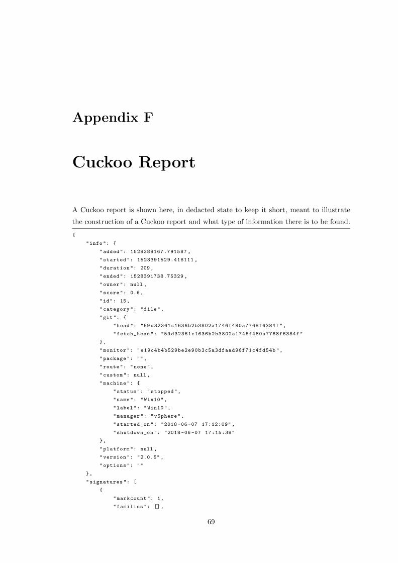
Appendix F

Cuckoo Report

A Cuckoo report is shown here, in dedacted state to keep it short, meant to illustrate

the construction of a Cuckoo report and what type of information there is to be found.

{

"info": {

"added": 1528388167.791587 ,

"started ": 1528391529.418111 ,

"duration ": 209,

"ended": 1528391738.75329 ,

"owner": null ,

"score": 0.6,

"id": 15,

"category ": "file",

"git": {

"head": "59 d32361c1636b2b3802a1746f480a7768f6384f",

"fetch_head ": "59 d32361c1636b2b3802a1746f480a7768f6384f"

},

"monitor ": "e19c4b4b529be2e90b3c5a3dfaad96f71c4fd54b",

"package ": "",

"route": "none",

"custom ": null ,

"machine ": {

"status ": "stopped",

"name": "Win10",

"label": "Win10",

"manager ": "vSphere",

"started_on ": "2018 -06 -07 17:12:09" ,

"shutdown_on ": "2018 -06 -07 17:15:38"

},

"platform ": null ,

"version ": "2.0.5" ,

"options ": ""

},

"signatures ": [

{

"markcount ": 1,

"families ": [],

69

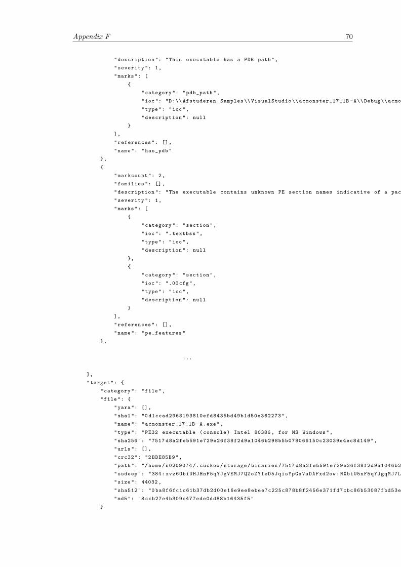
Appendix F 70

"description ": "This executable has a PDB path",

"severity ": 1,

"marks": [

{

"category ": "pdb_path",

"ioc": "D:\\ Afstuderen Samples \\ VisualStudio \\ acmonster_17_1B -A\\Debug\\ acmonster_17_1B -A.pdb",

"type": "ioc",

"description ": null

}

],

"references ": [],

"name": "has_pdb"

},

{

"markcount ": 2,

"families ": [],

"description ": "The executable contains unknown PE section names indicative of a packer (could be a false positive)",

"severity ": 1,

"marks": [

{

"category ": "section",

"ioc": ". textbss",

"type": "ioc",

"description ": null

},

{

"category ": "section",

"ioc": ".00 cfg",

"type": "ioc",

"description ": null

}

],

"references ": [],

"name": "pe_features"

},

...

],

"target ": {

"category ": "file",

"file": {

"yara": [],

"sha1": "0 d1ccad2968193810efd8435bd49b1d50e362273",

"name": "acmonster_17_1B -A.exe",

"type": "PE32 executable (console) Intel 80386 , for MS Windows",

"sha256 ": "7517 d8a2feb591e729e26f38f2d9a1046b298b5b078066150c23039e4ec8d149",

"urls": [],

"crc32": "2 BDE85B9",

"path": "/home/s0209074 /. cuckoo/storage/binaries /7517 d8a2feb591e729e26f38f2d9a1046b298b5b078066150c23039e4ec8d149",

"ssdeep ": "384: xvz6ObiUHJHnF5qYJgVEMJ7QZoZYIeD5JqisYpGxVuDAFxd2ow:NXbiU5nF5qYJgqMJ7LYD5EYpgUAFxs",

"size": 44032 ,

"sha512 ": "0 ba8f6fc1c61b37db2d00e16e9ee8ebee7c225c878b8f2456e371fd7cbc86b53087fbd53ebb3482df6a27b3ff8e402b9180a9b27b2be900f6f42dd27e1e5f038",

"md5": "8 ccb27e4b309c477ede0dd88b16435f5"

}

Appendix F 71

},

"network ": {

"tls": [],

"udp": [],

"dns_servers ": [],

"http": [],

"icmp": [],

"smtp": [],

"tcp": [],

"smtp_ex ": [],

"mitm": [],

"hosts": [],

"pcap_sha256 ": "704 e5e5b3234433c01fcfd1b20a306e77e985038120492dc53965c3edd38a4ea",

"dns": [],

"http_ex ": [],

"domains ": [],

"dead_hosts ": [],

"irc": [],

"https_ex ": []

},

"static ": {

"pdb_path ": "D:\\ Afstuderen Samples \\ VisualStudio \\ acmonster_17_1B -A\\Debug\\ acmonster_17_1B -A.pdb",

"pe_imports ": [

{

"imports ": [

{

"name": "? _Debug_message@std@@YAXPB_W0I@Z",

"address ": "0 x41c098"

}

],

"dll": "MSVCP140D.dll"

},

{

"imports ": [

{

"name": "__std_type_info_destroy_list",

"address ": "0 x41c0c8"

},

{

"name": "memset",

"address ": "0 x41c0cc"

},

...

],

"dll": "VCRUNTIME140D.dll"

},

...

],

"peid_signatures ": [

"Microsoft Visual C++ V8.0 (Debug)"

],

Appendix F 72

"keys": [],

"signature ": [],

"pe_timestamp ": "2018 -03 -21 12:08:37" ,

"pe_exports ": [],

"imported_dll_count ": 4,

"pe_imphash ": "0 ae46b28449b62f0bc1c219d0db52b01",

"pe_resources ": [

{

"name": "RT_MANIFEST",

"language ": "LANG_ENGLISH",

"filetype ": "XML 1.0 document text",

"sublanguage ": "SUBLANG_ENGLISH_US",

"offset ": "0 x0001e170",

"size": "0 x0000017d"

}

],

"pe_versioninfo ": [],

"pe_sections ": [

{

"size_of_data ": "0 x00000000",

"virtual_address ": "0 x00001000",

"entropy ": 0.0,

"name": ". textbss",

"virtual_size ": "0 x00010000"

},

{

"size_of_data ": "0 x00006800",

"virtual_address ": "0 x00011000",

"entropy ": 3.988371948793059 ,

"name": ".text",

"virtual_size ": "0 x00006745"

},

{

"size_of_data ": "0 x00002400",

"virtual_address ": "0 x00018000",

"entropy ": 2.0548363076464606 ,

"name": ".rdata",

"virtual_size ": "0 x0000231e"

},

...

]

},

"behavior ": {

"generic ": [

{

"process_path ": "C:\\ Windows \\ System32 \\lsass.exe",

"process_name ": "lsass.exe",

"pid": 512,

"summary ": {},

"first_seen ": 1528420574.437042 ,

"ppid": 448

}

],

Appendix F 73

"processes ": [

{

"process_path ": "C:\\ Windows \\ System32 \\lsass.exe",

"calls": [],

"track": false ,

"pid": 512,

"process_name ": "lsass.exe",

"command_line ": "C:\\ WINDOWS \\ system32 \\lsass.exe",

"modules ": [

{

"basename ": "lsass.exe",

"imgsize ": 53248,

"baseaddr ": "0 x2a0000",

"filepath ": "C:\\ WINDOWS \\ system32 \\lsass.exe"

},

{

"basename ": "ntdll.dll",

"imgsize ": 1638400 ,

"baseaddr ": "0 x775b0000",

"filepath ": "C:\\ WINDOWS \\ SYSTEM32 \\ntdll.dll"

},

...

],

"time": 16,

"tid": 3132,

"first_seen ": 1528420574.437042 ,

"ppid": 448,

"type": "process"

}

],

"processtree ": [

{

"track": false ,

"pid": 512,

"process_name ": "lsass.exe",

"command_line ": "C:\\ WINDOWS \\ system32 \\lsass.exe",

"first_seen ": 1528420574.437042 ,

"ppid": 448,

"children ": []

}

]

},

"debug": {

"action ": [

"gatherer"

],

"dbgview ": [],

"errors ": [],

"log": [

"2018 -06 -07 16:16:07 ,687 [analyzer] DEBUG: Starting analyzer from: C:\\ tmpiqlzku\n",

"2018 -06 -07 16:16:08 ,092 [analyzer] DEBUG: Pipe server name: \\??\\ PIPE\\ XGNwsbnvpmYdReloaQXrCfwoRK\n",

"2018 -06 -07 16:16:08 ,983 [analyzer] DEBUG: Log pipe server name: \\??\\ PIPE\\ QFvTrxypETnWRnnW\n",

"2018 -06 -07 16:16:09 ,529 [analyzer] DEBUG: No analysis package specified , trying to detect it automagically .\n",

Appendix F 74

"2018 -06 -07 16:16:09 ,608 [analyzer] INFO: Automatically selected analysis package \"exe\"\n",

"2018 -06 -07 16:16:10 ,592 [analyzer] DEBUG: Started auxiliary module DbgView\n",

...

"2018 -06 -07 16:16:29 ,124 [analyzer] INFO: Analysis completed .\n"

],

"cuckoo ": [

"2018 -06 -07 17:12:09 ,583 [cuckoo.core.scheduler] INFO: Task #15: acquired machine Win10 (label=Win10 )\n",

"2018 -06 -07 17:12:09 ,662 [cuckoo.auxiliary.sniffer] INFO: Started sniffer with PID 26074 (interface=virbr0 , host =192.168.56.101)\n",

"2018 -06 -07 17:12:09 ,672 [cuckoo.core.plugins] DEBUG: Started auxiliary module: Sniffer\n",

"2018 -06 -07 17:12:10 ,342 [cuckoo.machinery.vsphere] INFO: Reverting machine Win10 to snapshot Win10_snapshot2\n",

"2018 -06 -07 17:12:33 ,546 [cuckoo.core.guest] INFO: Starting analysis on guest (id=Win10 , ip =192.168.56.101)\n",

"2018 -06 -07 17:12:33 ,798 [cuckoo.core.guest] INFO: Guest is running Cuckoo Agent 0.8 (id=Win10 , ip =192.168.56.101)\n",

"2018 -06 -07 17:12:34 ,249 [cuckoo.core.guest] DEBUG: Uploading analyzer to guest (id=Win10 , ip =192.168.56.101 , monitor=latest , size =3840968)\n",

"2018 -06 -07 17:12:44 ,430 [cuckoo.core.guest] DEBUG: Win10: analysis still processing\n",

...

"2018 -06 -07 17:13:07 ,708 [cuckoo.core.guest] DEBUG: Win10: analysis still processing\n",

"2018 -06 -07 17:13:08 ,714 [cuckoo.core.guest] INFO: Win10: analysis completed successfully\n",

"2018 -06 -07 17:13:08 ,755 [cuckoo.core.plugins] DEBUG: Stopped auxiliary module: Sniffer\n",

"2018 -06 -07 17:13:09 ,024 [cuckoo.machinery.vsphere] INFO: Creating snapshot cuckoo_memdump_685128 for machine Win10\n",

"2018 -06 -07 17:13:39 ,099 [cuckoo.machinery.vsphere] INFO: Downloading memory dump [datastore1] Win10/Win10 -Snapshot366.vmem to /home/s0209074 /. cuckoo/storage/analyses /15/ memory.dmp\n",

"2018 -06 -07 17:15:27 ,805 [cuckoo.machinery.vsphere] INFO: Removing snapshot cuckoo_memdump_685128 for machine Win10\n",

"2018 -06 -07 17:15:37 ,610 [cuckoo.machinery.vsphere] INFO: Powering off virtual machine Win10\n",

"2018 -06 -07 17:15:38 ,726 [cuckoo.core.scheduler] DEBUG: Released database task #15\n",

"2018 -06 -07 17:15:38 ,792 [cuckoo.core.plugins] DEBUG: Executed processing module \" AnalysisInfo \" for task #15\n",

"2018 -06 -07 17:15:38 ,804 [cuckoo.core.plugins] DEBUG: Executed processing module \" BehaviorAnalysis \" for task #15\n",

...

"2018 -06 -07 17:15:39 ,693 [cuckoo.core.plugins] DEBUG: Executed processing module \"Debug\" for task #15\n",

"2018 -06 -07 17:15:39 ,699 [cuckoo.core.plugins] DEBUG: Running 540 signatures\n",

"2018 -06 -07 17:15:39 ,960 [cuckoo.core.plugins] DEBUG: Analysis matched signature: has_pdb\n",

"2018 -06 -07 17:15:39 ,963 [cuckoo.core.plugins] DEBUG: Analysis matched signature: pe_features\n",

"2018 -06 -07 17:15:39 ,965 [cuckoo.core.plugins] DEBUG: Analysis matched signature: peid_packer\n"

]

},

"strings ": [

"!This program cannot be run in DOS mode.",

". textbss",

"‘.rdata",

"@.data",

".idata",

"@.00 cfg",

"@.rsrc",

"@.reloc",

"Case #%d: %0.10 lf",

...

"Changing the code in this way will not affect the quality of the resulting optimized code.",

"Stack memory was corrupted",

...

"Data: <",

"Allocation number within this function: ",

"Size: ",

"Address: 0x",

"Stack area around _alloca memory reserved by this function is corrupted",

"%s%s%p%s%zd%s%d%s%s%s%s%s",

"A variable is being used without being initialized .",

...

Appendix F 75

"RegOpenKeyExW",

"RegQueryValueExW",

"RegCloseKey",

"PDBOpenValidate5",

"RSDSpX",

"D:\\ Afstuderen Samples \\ VisualStudio \\ acmonster_17_1B -A\\Debug \\ acmonster_17_1B -A.pdb",

"? _Debug_message@std@@YAXPB_W0I@Z",

"MSVCP140D.dll",

...

"_c_exit",

"_register_thread_local_exe_atexit_callback",

"_configthreadlocale",

"_set_new_mode",

"__p__commode",

"strcpy_s",

"strcat_s",

...

"ucrtbased.dll",

"IsDebuggerPresent",

"RaiseException",

"MultiByteToWideChar",

"WideCharToMultiByte",

"GetCurrentProcess",

...

"KERNEL32.dll",

"<?xml version =’1.0’ encoding=’UTF -8’ standalone=’yes ’?>",

"<assembly xmlns=’urn:schemas -microsoft -com:asm.v1’ manifestVersion =’1.0’>",

" <trustInfo xmlns =\"urn:schemas -microsoft -com:asm.v3\">",

" <security >",

" <requestedPrivileges >",

...

"3\"3(3.343" ,

"8 8p<|?",

"c:\\ program files (x86)\\ microsoft visual studio \\2017\\ community \\vc\\tools\\msvc \\14.13.26128\\ include \\ xutility",

"c:\\ program files (x86)\\ microsoft visual studio \\2017\\ community \\vc\\tools\\msvc \\14.13.26128\\ include \\ algorithm",

"invalid comparator",

"std:: _Debug_lt_pred",

"\" invalid comparator \"",

"Runtime Check Error.",

" Unable to display RTC Message.",

"Run -Time Check Failure #%d - %s",

"bin\\ MSPDB140.DLL",

"VCRUNTIME140D.dll",

"api -ms -win -core -registry -l1 -1-0.dll",

"advapi32.dll",

"SOFTWARE \\ Wow6432Node \\ Microsoft \\ VisualStudio \\14.0\\ Setup \\VC",

..

"MSPDB140"

],

"metadata ": {

"output ": {

"pcap": {

"basename ": "dump.pcap",

"sha256 ": "704 e5e5b3234433c01fcfd1b20a306e77e985038120492dc53965c3edd38a4ea",

"dirname ": ""

Appendix F 76

}

}

}

}

Appendix G

Results Experiment 2

The following table shows the amount of features found in the Cuckoo reports in the

form of information points. An information point signifies the presence of a feature. For

the obfuscated versions of a sample 1/2 points were deducted when a feature is present

but altered from the non-obfuscated version. The points are presented in two parts, the

first counting static features and the second counting dynamic features.

77

Appendix G 78

No obfuscation UPX Themida StunnixStatic Dynamic Static Dynamic Static Dynamic Static Dynamic

acmonster 17 1B-A 510 387 215 387 3288 18323 514 387

acmonster 17 1B-C 518 387 227 387 3196 17125 518 387

acmonster 17 2-A 509 387 - - 3264 13363 511 387

acmonster 17 2-D 493 387 227 387 3322 18537 505 387

acmonster 17 Q-C 684 387 263 387 3230 15703 684 387

ania7 17 1B-A 562 387 230 387 3458 21354 572 387

ania7 17 1B-C 553 387 226 387 3208 16011 565 387

ania7 17 2-A 555 387 230 387 3288 18023 556 387

ania7 17 2-D 713 387 288 387 3288 17626 725 387

ania7 17 Q-C 667 387 258 387 3356 18818 670 387

burunduk1 17 1B-A 635 387 229 387 3366 17271 635 387

burunduk1 17 1B-C 577 387 225 387 3298 16617 581 387

burunduk1 17 2-A 627 387 222 387 3094 14261 630 387

burunduk1 17 2-D 714 387 294 387 3264 14361 - -

burunduk1 17 Q-C 658 387 248 387 3434 16481 656 387

matthew99 17 1B-A 550 387 228 387 3458 17999 549 387

matthew99 17 1B-C 550 387 225 387 3332 15165 558 387

matthew99 17 2-A 695 387 273 387 3344 16371 704 387

matthew99 17 2-D 673 387 273 387 3332 15057 - -

matthew99 17 Q-C 671 387 277 387 3264 17529 674 387

nika 17 1B-A 556 387 215 387 3230 15923 556 387

nika 17 1B-C 660 387 261 387 3332 16677 662 387

nika 17 2-A 551 387 242 387 3344 17800 551 387

nika 17 2-D 801 387 306 387 3288 18254 801 387

nika 17 Q-C 762 387 289 387 3322 17372 772 387

nullstellensatz 17 1B-A 620 387 239 387 3300 14430 629 387

nullstellensatz 17 1B-C 616 387 260 387 3344 16514 621 387

nullstellensatz 17 2-A 603 387 242 387 3368 21063 608 387

nullstellensatz 17 2-D 698 387 269 387 3332 14846 697 387

nullstellensatz 17 Q-C 721 387 261 387 3322 18718 723 387

pasqual45 17 1B-A 986 387 283 387 3424 15541 982 387

pasqual45 17 1B-C 1004 387 303 387 3162 16315 620 387

pasqual45 17 2-A 963 387 294 387 3366 17085 966 387

pasqual45 17 2-D 1052 387 323 387 3366 14775 1062 387

pasqual45 17 Q-C 978 387 302 387 3400 16509 979 387

simonlindholm 17 1B-A 674 387 235 387 3196 14754 673 387

simonlindholm 17 1B-C 764 387 291 387 3332 14936 770 387

simonlindholm 17 2-A 755 387 263 387 3402 20604 - -

simonlindholm 17 2-D 921 387 335 387 3332 16996 - -

simonlindholm 17 Q-C 757 387 275 387 3434 16050 762 387

xellos 17 1B-A 745 387 275 387 3220 16333 758 387

xellos 17 1B-C 784 387 278 387 3322 17397 799 387

xellos 17 2-A 647 387 254 387 3126 17107 651 387

xellos 17 2-D 867 387 298 387 3230 14871 884 387

xellos 17 Q-C 758 387 275 387 3174 16977 764 387

Table G.1: Information points of each of the samples run in Cuckoo

Bibliography

[1] Kim Zetter. Countdown to Zeroday. Crown Publishers, New York, 2014.

[2] R. McArdle. Mcardle malware analysis lectures 2016. 2016.

[3] Reverse engineering, 2016. URL https://satyamsmagicalmind.weebly.com/

blog/category/all.

[4] Symantec Corporation. Pc or mac: Which is more resistant to cyber threats?, 2018.

URL https://us.norton.com/internetsecurity-malware-pc-or-mac.html.

[5] How to use windows api knowledge to be a better defender, 2017. URL https:

//redcanary.com/blog/windows-technical-deep-dive/.

[6] Randy Abrams. An introduction to packers, 2008. URL https://www.

welivesecurity.com/2008/10/27/an-introduction-to-packers/.

[7] Malware packers use tricks to avoid analysis, detection,

2017. URL http://www.impingtoncomputers.co.uk/blog/

malware-packers-use-tricks-to-avoid-analysis-detection/.

[8] Pieter Arntx. Explained: Packer, crypter, and protector, 2017.

URL https://blog.malwarebytes.com/cybercrime/malware/2017/03/

explained-packer-crypter-and-protector/.

[9] URL http://stunnix.com/prod/cxxo/.

[10] Aylin Caliskan-Islam, Richard Harang, Andrew Liu, Arvind Narayanan, Clare Voss,

Fabian Yamaguchi, and Rachel Greenstadt. De-anonymizing programmers via code

stylometry. In 24th USENIX Security Symposium (USENIX Security), Washington,

DC, 2015.

[11] Aylin Caliskan-Islam, Fabian Yamaguchi, Edwin Dauber, Richard Harang, Konrad

Rieck, Rachel Greenstadt, and Arvind Narayanan. When coding style survives com-

pilation: De-anonymizing programmers from executable binaries. arXiv preprint

arXiv:1512.08546, 2015.

79

Bibliography 80

[12] M Sudheep Elayidom, Chinchu Jose, Anitta Puthussery, and Neenu K Sasi. Text

classification for authorship attribution analysis. arXiv preprint arXiv:1310.4909,

2013.

[13] Marcelo Luiz Brocardo, Issa Traore, Sherif Saad, and Isaac Woungang. Authorship

verification for short messages using stylometry. In Computer, Information and

Telecommunication Systems (CITS), 2013 International Conference on, pages 1–6.

IEEE, 2013.

[14] Aziz Mohaisen, Omar Alrawi, and Manar Mohaisen. Amal: High-fidelity, behavior-

based automated malware analysis and classification. Computers & Security, 2015.

[15] Shanhu Shang, Ning Zheng, Jian Xu, Ming Xu, and Haiping Zhang. Detecting mal-

ware variants via function-call graph similarity. In Malicious and Unwanted Soft-

ware (MALWARE), 2010 5th International Conference on, pages 113–120. IEEE,

2010.

[16] Rayan Mosli, Rui Li, Bo Yuan, and Yin Pan. Automated malware detection using

artifacts in forensic memory images. In Technologies for Homeland Security (HST),

2016 IEEE Symposium on, pages 1–6. IEEE, 2016.

[17] Jidong Xiao, Lei Lu, Haining Wang, and Xiaoyun Zhu. Hyperlink: Virtual machine

introspection and memory forensic analysis without kernel source code. In Auto-

nomic Computing (ICAC), 2016 IEEE Internation Conference on, pages 127–136.

IEEE, 2016.

[18] Brendan Dolan-Gavitt, Tim Leek, Michael Zhivich, Jonathon Giffin, and Wenke

Lee. Virtuoso: Narrowing the semantic gap in virtual machine introspection. In

Security and Privacy (SP), 2011 IEEE Symposium on, pages 297–312. IEEE, 2011.

[19] Cuckoo Foundation. Cuckoo, 2016. URL https://www.cuckoosandbox.org.

[20] What is cuckoo?, 2016. URL https://cuckoo.sh/docs/introduction/what.

html.

[21] How to choose algorithms for microsoft azure machine learning, 2017.

URL https://docs.microsoft.com/en-us/azure/machine-learning/studio/

algorithm-choice.

[22] Essentials of machine learning algorithms (with python and r codes),

2017. URL https://www.analyticsvidhya.com/blog/2015/08/

common-machine-learning-algorithms/.

[23] The UPX Team. Upx, 2017. URL https://upx.github.io/.

Bibliography 81

[24] Upx, 2017. URL https://en.wikipedia.org/wiki/UPX.

[25] Michael Sikorski and Andres Honig. Practical Malware Analysis. no starch press,

2012.