Corrections Involving the Spearman Correlation Coefficient: Sections 7.1.2 and 7.1.6

7.1.2 Spearman Correlation Coefficient

The Spearman correlation coefficient is a measure of the strength of the monotonic relationship

in a sample of pairs. A monotonic relationship exists when one variable tends to increase or

decrease with respect to the other variable. A linear relationship is a type of monotonic

relationship.

The Spearman correlation coefficient is the Pearson correlation coefficient applied to the ranks of

the data. It is represented by sr .

1

1 1

2 2

1

n

i i

i

s

r x r y

n nr x r y

rn s s

ir x : the rank of ix r x

s : the standard deviation of the ranks of ix

ir y : the rank of iy r ys : the standard deviation of the ranks of iy

Ranks correspond to the positions data would have if sorted from smallest to largest. Tied values

are given average ranks, called midranks. The mean of the ranks is 1 2n . For example:

45, 68, 33, 53, 70 have ranks 2, 4, 1, 3, 5. The mean of the ranks is 3.

45, 68, 33, 45, 70 have ranks 2.5, 4, 1, 2.5, 5. The mean of these ranks is 3.

The Spearman correlation coefficient is less sensitive to outlying pairs than the Pearson. Data

points based on ranks keep much of the original pattern but limit the effects of outliers. See

Figure 7.6.

(a) shows a scatter plot of a sample. There are no outliers: no points unusually far from

the other data points. The statistics and sr r are below the scatter plots. The two values

are close.

(b) shows a scatter plot of the data points based on the ranks of the data. Technically, sr

is the Pearson correlation coefficient of the data points in (b).

The scatter plots are similar. This is reflected in and sr r being similar. The r statistic is

preferred because it is based on the original data.

Figure 7.6 (a) Scatter Plot of data, (b) Scatter Plot Based on Ranks

(a) (b)

0.84886

-value 0.0001

r

p

0.88277

-value 0.0001

sr

p

The sample plotted in Figure 7.7 (a) contains an outlier.

With r = 0.05417 and the p-value = 0.8206, the interpretation is that there is no

significant linear correlation in the sample. However, the outlier has increased the

standard deviations and x ys s so much that they mask the correlation that does exist.

The outlier still exists among the data points based on ranks in (b), but its impact is much

smaller. With sr = 0.57143 and the p-value = 0.0085, there is a significant increasing

relationship between the paired values in the sample.

Figure 7.7 (a) Scatter Plot of Data with Outlier, (b) Scatter Plot Based on Ranks

(a) (b)

outlier

0.05417

-value 0.8206

r

p

0.57143

-value 0.0085

sr

p

An increasing relationship is present in the data when 0sr and sr is significantly different from

0. Significance is a result of the test discussed in “Hypothesis Test with the Spearman Correlation

Coefficient.” See Table 7.4. With an increasing relationship, smaller x values tend to be paired

with smaller y values and larger x values with larger y values. The closer sr is to 1, the stronger

this tendency.

A decreasing relationship is present in the data when 0sr and sr is significantly different from

0. In this case, smaller x values tend to be paired with larger y values and larger x values with

smaller y values. The closer sr is to −1, the stronger this tendency.

No monotonic relationship is present in the data when sr is not significantly different from 0. In

this case, both smaller and larger x values tend to be paired with smaller y values and with larger

y values.

7.1.2.1 Hypothesis Test with the Spearman Correlation Coefficient

This is a test on whether there is a monotonic relationship between the paired random variables X

and Y. It is a nonparametric test: it is not a test regarding a parameter. The null and alternative

hypotheses are:

0

1

:There is no monotonic relationship between and .

:There is a monotonic relationship between and .

H X Y

H X Y

The same form of the t Value is used with both the Spearman and Pearson correlation

coefficients:

2

0 Value

1

2

s

s

rt

r

n

In terms of 0H , the p-value is the probability that a random sample from a population where

there is no monotonic relationship between the paired values would produce a t Value at or

beyond the current value. If the p-value is small, it is unlikely that the current sample comes from

a population where there is no monotonic relationship between the paired values.

The technical definition of the p-value is in Table 7.4. The random variable T represents a future

value of the test statistic and follows the t distribution with n − 2 degrees of freedom. In the SAS

code expression, the t Value and n − 2 represent numbers. The SAS code expression is included

to aid in the discussion. The p-value is computed using the expression in the “Detailed Solutions”

section of “Example 7.2: Spearman Correlation Coefficients.”

Table 7.4 p-Value for Hypothesis Test with the Spearman Correlation Coefficient

Hypotheses Gray area corresponds to the probability statement and is an example.

0

1

: There is no ...

relationship ....

: There is ...

relationship ....

H

H

-value 2 Valuep P T t

Task output:

-value

sr

p

SAS code expression:

2*(1-probt(abs(t Value),n − 2))

Decision and Conclusions The formal decision and concluding sentence do not change from the one-sample tests discussed

in Chapter 4, “Inferences from One Sample.” The concluding observation depends on the

particular statistics involved in the test.

If the p-value is small, the data agrees with H1. If the p-value is less than the significance level,

the risk of making a Type I error is acceptable. Therefore, the p-value decision rule is the

following:

If the p-value < α, reject H0. Otherwise, do not reject H0.

Since a hypothesis test begins with the assumption that H0 is true, concluding a hypothesis test

requires one of the following formal statements:

Reject H0.

Do not reject H0.

When the claim is equivalent to the null hypothesis, the concluding sentence uses the word reject.

The concluding sentence becomes an expanded version of the formal decision.

When the claim is equivalent to the alternative hypothesis, the concluding sentence uses the word

support. If the data supports the rejection of H0, the data supports H1. If the data does not support

the rejection of H0, the data cannot support H1.

Table 7.5 Concluding Sentences

Formal Statistical

Decision Claim stated as H0 Claim stated as H1

Reject H0.

There is sufficient evidence to reject

the claim that ... (claim in words).

There is sufficient evidence to

support the claim that ... (claim in

words).

Do not reject H0.

There is not sufficient evidence to

reject the claim that ... (claim in

words).

There is not sufficient evidence to

support the claim that ... (claim in

words).

Table 7.6 Concluding Observations

Reject H0.

< 0sr > 0sr

There is a significant decreasing

relationship between variables.

There is a significant increasing

relationship between the variables.

Do not reject H0.

There is no significant increasing or decreasing relationship between the

variables.

7.1.2.2 Spearman Partial Correlation Coefficient

The Spearman partial correlation coefficient is the Pearson partial correlation coefficient applied

to the ranks of the data. The Spearman partial correlation coefficient of the variables w and y that

controls the effect of the variable x is represented by .s wy xr

It is computed with the w-y, w-x, y-

x Spearman correlation coefficients: , ,s swy wxr r and .s yx

r

2 2

1 1

s s swy wx yx

s wy x

s swx yx

r r rr

r r

The hypothesis test is whether there is a monotonic relationship between the paired random

variables W and Y with the effect of the random variable X being controlled. It is a nonparametric

test: it is not a test regarding a parameter. The null and alternative hypotheses are:

0

1

:There is no monotonic relationship between and when the effect is controlled.

:There is a monotonic relationship between and when the effect is controlled.

H W Y X

H W Y X

The test statistic follows the Student’s t distribution with 3n degrees of freedom:

2

0 Value

1

3

s wy x

s wy x

rt

r

n

7.1.6 Example 7.2: Spearman Correlation Coefficients

Example 7.2 applies the Spearman correlation coefficient as a descriptive statistic and as a basis

for inference on the population of paired values. The requested analysis includes a number of

Spearman and Pearson correlation coefficients, hypothesis tests, and scatter plots. The Spearman

correlation coefficients and the hypothesis tests are worked out in the “Detailed Solutions”

section.

7.1.6.1 Student Data with Outlier

Student Midterm Final Absent

1 64 63 5

2 64 68 5

3 66 68 4

4 68 72 3

5 72 69 5

6 73 80 3

7 78 74 2

8 81 85 3

9 91 96 2

10 92 90 3

11 94 72 25

Note that an eleventh student has been added to the data in Example 7.1.

These values are in the Ex07_02 data set. The variable names are as shown in the table: Midterm,

Final, and Absent.

Example 7.2.1 Determine the Spearman and Pearson correlation coefficients for the following pairs of

measurements:

a. midterm and final exam scores

b. final exam score and numbers of absences

Example 7.2.2 Use the Spearman correlation coefficient to test the claim that, among all students who take this

particular course, there is a monotonic relationship between the midterm exam score and the final

exam score. Let α = 0.05.

Example 7.2.3 Use the Spearman correlation coefficient to test the claim that, among all students who take this

particular course, there is a monotonic relationship between the final exam score and the number

of absences. Let α = 0.05.

Example 7.2.4 Construct a scatter plot for the midterm and final exam scores and a scatter plot for the final exam

scores and the numbers of absences. On each plot, identify the data point associated with the

eleventh student.

7.1.6.2 Detailed Solutions

Example 7.2.1 For the Midterm and Final scores:

Midterm Final

x y r x r y + 1

-2

nr x

+ 1-

2

nr y 1

2

2

n +r x -

2

1-

2

n +r y

1 1

2 2

n + n +r x - r y -

64 63 1.5 1 -4.5 -5 20.25 25 22.5

64 68 1.5 2.5 -4.5 -3.5 20.25 12.25 15.75

66 68 3 2.5 -3 -3.5 9 12.25 10.5

68 72 4 5.5 -2 -0.5 4 0.25 1

72 69 5 4 -1 -2 1 4 2

73 80 6 8 0 2 0 4 0

78 74 7 7 1 1 1 1 1

81 85 8 9 2 3 4 9 6

91 96 9 11 3 5 9 25 15

92 90 10 10 4 4 16 16 16

94 72 11 5.5 5 -0.5 25 0.25 -2.5

sums: 66 66 0 0 109.5 109 87.25

1

1

1

109.5211 3.30908

1 10

1

10923.30151

1 10

n

i

i

r x

n

i

i

r y

nr x

n sn

nr y

sn

1

1 1

2 2

1

87.25

11 1 3.30908 3.30151

0.79863

n

i i

is

r x r y

n nr x r y

rn s s

For the Final and Absent scores:

Final Absent

x y r x r y 1

2

n +r x -

1

2

n +r y -

2

n + 1-

2r x

2

+ 1-

2

nr y

+ 1 + 1- -

2 2

n nr x r y

63 5 1 9 -5 3 25 9 -15

68 5 2.5 9 -3.5 3 12.25 9 -10.5

68 4 2.5 7 -3.5 1 12.25 1 -3.5

72 3 5.5 4.5 -0.5 -1.5 0.25 2.25 0.75

69 5 4 9 -2 3 4 9 -6

80 3 8 4.5 2 -1.5 4 2.25 -3

74 2 7 1.5 1 -4.5 1 20.25 -4.5

85 3 9 4.5 3 -1.5 9 2.25 -4.5

96 2 11 1.5 5 -4.5 25 20.25 -22.5

90 3 10 4.5 4 -1.5 16 2.25 -6

72 25 5.5 11 -0.5 5 0.25 25 -2.5

sums: 66 66 0 0 109 102.5 -77.25

1

1

1

109211 3.30151

1 10

1

102.523.20156

1 10

n

i

i

r x

n

i

i

r y

nr x

n sn

nr y

sn

1

1 1

2 2

1

77.25

11 1 3.30151 3.20156

0.73084

n

i i

is

r x r y

n nr x r y

rn s s

Example 7.2.2

Plan the task.

0

1

: There is no monotonic relationship between the midterm exam score and the final exam score.

: There is a monotonic relationship between the midterm exam score and the final exam score.

H

H

Compute the statistics.

2 2

0 0.79863 Statistic 3.9811

1 1 0.79863

2 11 2

s

s

rt

r

n

Since 3.9811 is positive, the absolute value function can be dropped:

-value 2 3.9811 2*(1- probt(3.9811,9)) 0.0032p P T

Apply the results.

Since the p-value < 0.05, reject H0. There is sufficient evidence to support the claim that, among

all students who take this particular course, there is a monotonic relationship between the

midterm exam score and the final exam score. There is a significant increasing relationship

between the midterm and the final exam scores in the sample.

Example 7.2.3

Plan the task.

0

1

: There is no monotonic relationship between the final exam score and the number of absences.

: There is a monotonic relationship between the final exam score and the number of absences.

H

H

Compute the statistics.

2 2

0 0.73084 Statistic 3.2123

1 1 0.73084

2 10 2

s

s

rt

r

n

-value 2 3.2123 2*(1- probt(abs(-3.2123),8)) 0.01062p P T

Apply the results.

Since the p-value < 0.05, reject H0. There is sufficient evidence to support the claim that, among

all students who take this particular course, there is a monotonic relationship between the final

exam score and the number of absences. There is a significant decreasing relationship between

the final exam scores and the numbers of absences in the sample.

7.1.6.3 Correlations Task

The following task selections are different from Example 7.1:

The active data is Ex07_02.

Task Roles

o Midterm and Absent are assigned to Analysis variables.

o Final is assigned to Correlate with.

Options: Both Pearson and Spearman are selected.

7.1.6.4 Task Output, Interpretation, and Analysis

Task output

Output 7.3 Correlations Output for Example 7.2

Correlation Analysis

The CORR Procedure

1 With Variables: Final

2 Variables: Midterm Absent

Simple Statistics

Variable N Mean Std Dev Median Minimum Maximum

Final 11 76.09091 10.36778 72.00000 63.00000 96.00000

Midterm 11 76.63636 11.43042 73.00000 64.00000 94.00000

Absent 11 5.45455 6.57820 3.00000 2.00000 25.00000

Pearson Correlation Coefficients, N = 11

Prob > |r| under H0: Rho=0

Midterm Absent

Final 0.73612 0.0098

-0.25286 0.4531

Spearman Correlation Coefficients, N = 11

Prob > |r| under H0: Rho=0

Midterm Absent

Final 0.79863 0.0032

-0.73084 0.0106

Scatter plot of Midterm by Final

Final = 72 and

Midterm = 94

for the 11th student

Scatter plot of Final by Absent

Interpretation & indicate how the results are read:

The top number is the Pearson correlation coefficient r.

The second number is the p-value of the hypothesis test on 0 : 0H .

Each pair of variables involves n = 11 pairs of values.

For Midterm and Final, r = 0.73612 and the p-value = 0.0098.

For Final and Absent, r = −0.25286 and the p-value = 0.4531.

& indicate how the results are read:

The top number is the Spearman correlation coefficient sr .

The second number is the p-value of the hypothesis test.

For Midterm and Final, sr = 0.79863 and the p-value = 0.0032.

For Final and Absent, sr = −0.73084 and the p-value = 0.0106.

Scatter plot for Midterm and Final

Scatter plot for Final and Absent

Analysis

Example 7.2.1

Spearman correlation

coefficients

Pearson correlation

coefficients

midterm and final exam scores sr = 0.79863

See in Output 7.3.

r = 0.73612

See in Output 7.3.

final exam score and number of

absences sr = −0.73084 r = −0.25286

See in Output 7.3.

11

11

Final = 72

and Absent = 25

for the 11th student

See in Output 7.3.

Example 7.2.2

0

1

: There is no monotonic relationship between the midterm exam score and the final exam score.

: There is a monotonic relationship between the midterm exam score and the final exam score.

H

H

p-value = 0.0032. See in Output 7.3.

Since the p-value < 0.05, reject H0. There is sufficient evidence to support the claim that, among

all students who take this particular course, there is a monotonic relationship between the

midterm exam score and the final exam score. There is a significant increasing relationship

between the midterm and the final exam scores in the sample.

Example 7.2.3

0

1

: There is no monotonic relationship between the final exam score and the number of absences.

: There is a monotonic relationship between the final exam score and the number of absences.

H

H

p-value = 0.0106. See in Output 7.3.

Since the p-value < 0.05, reject H0. There is sufficient evidence to support the claim that, among

all students who take this particular course, there is a monotonic relationship between the final

exam score and the number of absences. There is a significant decreasing relationship between

the final exam scores and the numbers of absences in the sample.

Example 7.2.4

See and in Output 7.3.

7.1.7 Example 7.3: Partial Correlation Coefficients

7.1.7.1 Reading Assessment, Homework, and Age

In a particular school district, reading assessment tests are given to students in three age groups:

9, 13, and 17. The scores are standardized so that comparisons can be made between groups. Four

students from each group are randomly selected. The typical number of pages read daily in class

and homework is determined for each student. The results are below.

11

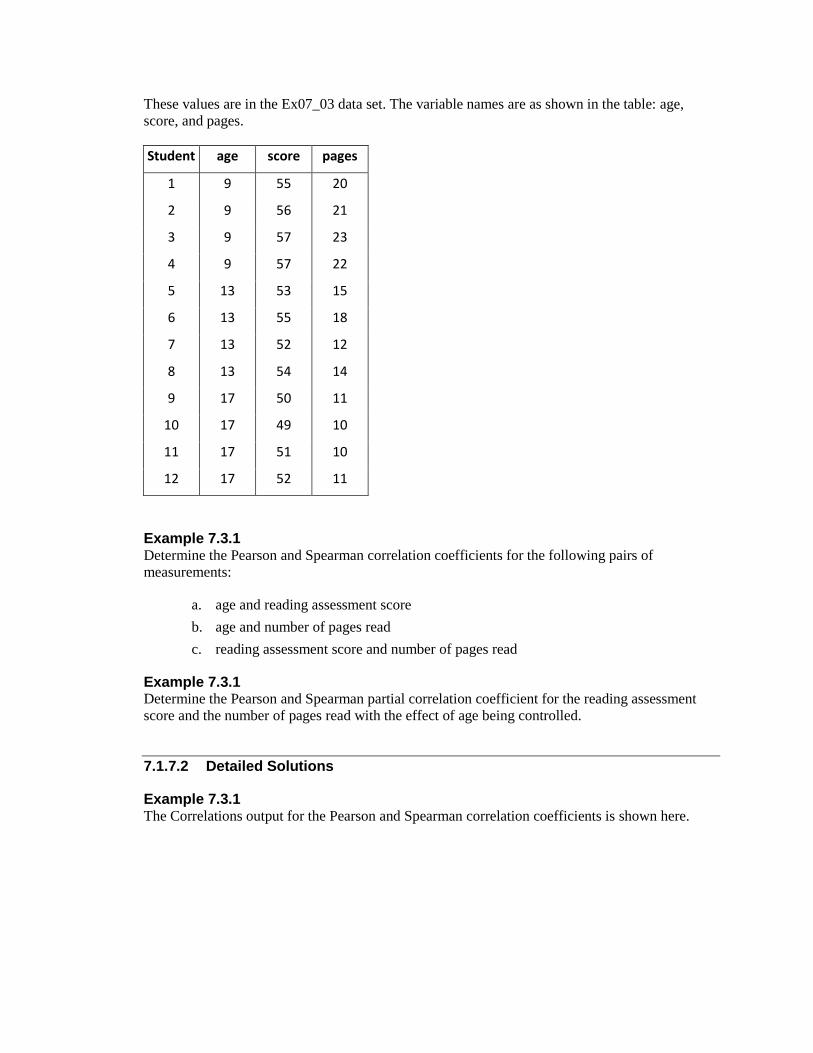
These values are in the Ex07_03 data set. The variable names are as shown in the table: age,

score, and pages.

Student age score pages

1 9 55 20

2 9 56 21

3 9 57 23

4 9 57 22

5 13 53 15

6 13 55 18

7 13 52 12

8 13 54 14

9 17 50 11

10 17 49 10

11 17 51 10

12 17 52 11

Example 7.3.1 Determine the Pearson and Spearman correlation coefficients for the following pairs of

measurements:

a. age and reading assessment score

b. age and number of pages read

c. reading assessment score and number of pages read

Example 7.3.1 Determine the Pearson and Spearman partial correlation coefficient for the reading assessment

score and the number of pages read with the effect of age being controlled.

7.1.7.2 Detailed Solutions

Example 7.3.1 The Correlations output for the Pearson and Spearman correlation coefficients is shown here.

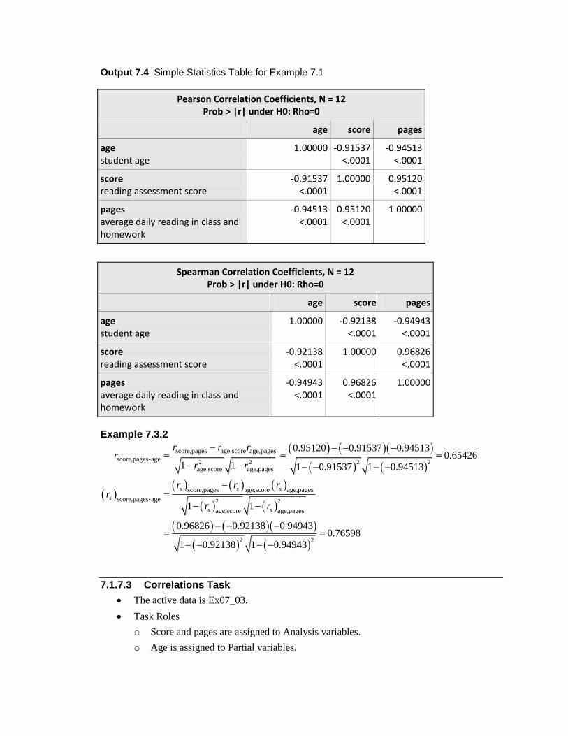
Output 7.4 Simple Statistics Table for Example 7.1

Pearson Correlation Coefficients, N = 12 Prob > |r| under H0: Rho=0

age score pages

age student age

1.00000

-0.91537 <.0001

-0.94513 <.0001

score reading assessment score

-0.91537 <.0001

1.00000

0.95120 <.0001

pages average daily reading in class and homework

-0.94513 <.0001

0.95120 <.0001

1.00000

Spearman Correlation Coefficients, N = 12 Prob > |r| under H0: Rho=0

age score pages

age student age

1.00000

-0.92138 <.0001

-0.94943 <.0001

score reading assessment score

-0.92138 <.0001

1.00000

0.96826 <.0001

pages average daily reading in class and homework

-0.94943 <.0001

0.96826 <.0001

1.00000

Example 7.3.2

2 2 2 2

2

score,pages age,score age,pages

score,pages age

age,score age,pages

score,pages age,score age,pages

score,pages age

age,score

0.95120 0.91537 0.945130.65426

1 1 1 0.91537 1 0.94513

1 1

s s s

s

s

r r rr

r r

r r rr

r

2

2 2

age,pages

0.96826 0.92138 0.949430.76598

1 0.92138 1 0.94943

sr

7.1.7.3 Correlations Task

The active data is Ex07_03.

Task Roles

o Score and pages are assigned to Analysis variables.

o Age is assigned to Partial variables.

Options: Both Pearson and Spearman are selected.

7.1.7.4 Task Output and Interpretation

Task Output

Output 7.5 Correlations Output for Example 7.3.2

Correlation Analysis

The CORR Procedure

1 Partial Variables: age

2 Variables: score pages

Simple Statistics

Variable N Mean Std Dev Median Minimum Maximum Partial

Variance Partial

Std Dev

age 12 13.00000 3.41121 13.00000 9.00000 17.00000

score 12 53.41667 2.67848 53.50000 49.00000 57.00000 1.27917 1.13100

pages 12 15.58333 4.96274 14.50000 10.00000 23.00000 2.89167 1.70049

Label

student age

reading assessment score

average daily reading in class and homework

Pearson Partial Correlation Coefficients, N = 12 Prob > |r| under H0: Partial Rho=0

score pages

score reading assessment score

1.00000

0.65427 0.0290

pages average daily reading in class and homework

0.65427 0.0290

1.00000

Spearman Partial Correlation Coefficients, N = 12 Prob > |r| under H0: Partial Rho=0

score pages

score reading assessment score

1.00000

0.76595 0.0060

pages average daily reading in class and homework

0.76595 0.0060

1.00000

Interpretation The partial variance is equal to the Error Mean Square, MS(Error), in the linear regression

analysis of variance table with the controlled variable(s) as the explanatory variable(s).

For simple linear regression with score as the dependent variable and age as the

explanatory variable, MS(Error) = 1.27917. With pages as the dependent variable and age

as the explanatory variable, MS(Error) = 2.89167.

The partial standard deviation is ErrorMS .

The Pearson partial correlation coefficient for the reading assessment score and the

number of pages read with the effect of age being controlled is 0.65427.

The Spearman partial correlation coefficient for the reading assessment score and the

number of pages read with the effect of age being controlled is 0.76595.