Correct Interpretation of sorption mechanism by Isothermal ... · Correct Interpretation of...
15
IJCBS, 12(2017):53-67 Hanif et al., 2017 53 Correct Interpretation of sorption mechanism by Isothermal, Kinetic and Thermodynamic models Muhammad Asif Hanif ٭1 , Hafiz Muhammad Tauqeer 2 , Nabiha Aslam 1 , Asma Hanif 1 , Muhammad Yaseen 3 and Rasheed Ahmad Khera 1 1 Department of Chemistry, University of Agriculture, Faisalabad-38040-Pakistan, 2 Department of Environmental Sciences, Hafiz Hayat Campus, Jalal Pur Jattan Road, 50700, Gujrat, Pakistan, 3 Department of Mathematics and Statics, University of Agriculture, Faisalabad-38040-Pakistan Abstract A number of kinetic and isothermal models have been used by various researchers to interpret mechanisms involved behind sorption process. However, a careful review of literature shows that several times researchers have withdrawn wrong conclusions due to unawareness about postulates of models as well as regarding correct mathematical and statistical parameters. This review article presents the overall picture about the adsorption isotherms modeling, their fundamental characteristics and mathematical expressions. Furthermore, kinetic modeling and rate equations are also described in details with their mathematical expressions. There is need to develop suitable correlations for batch and continuous equilibrium data using theoretical or empirical equations that are key component in predictive modeling methods for the analysis and design of adsorption system. In conclusion, this single review will provide complete understanding of all models applicable to sorption data and will provide complete understanding to enable researcher to select correct model for explanation of the results of adsorption experiments. Key words: Theoretical models, Adsorption, Wastewater Treatment Full length article *Corresponding Author, e-mail: [email protected] 1. Introduction 1.1 Adsorption Isotherm Adsorption is a process in which solute particles are isolated from liquid phase with a solid adsorbent having specific affinity for a particular solute particle. Generally, adsorption processes are economically acceptable due to easy availability of sorbents, reduced cost and lower volume of the sludge for handling and disposal, recovery/extraction of metals from the absorbent and reuse of adsorbents for further treatments. Different natural, ecofriendly and synthetic adsorbents have been used for the removal of heavy metals (Cd 2+ , Pb 2+ , Ni 2+ , As 3+ and As 5+ ) by numerous researchers [1, 2]. The success of adsorption isotherm depends upon the amount of adsorbate per unit weight of the adsorbent and the concentration of adsorbate in the solution at a specific temperature and equilibrium conditions. Empirical or theoretical equations play key role in predictive modeling procedures to understand and analyze the design of adsorption systems. There is need to develop a strong and appropriate correlations for the batch equilibrium data by using empirical or theoretical equations [2]. In general, adsorption isotherm is valuable curve explaining the release or movement phenomenon of substance from aqueous medium to a solid state at a specific pH and constant temperature. Adsorption equilibrium is developed when an adsorbate have a contact with the adsorbent for a plenty of time, with the concentration of adsorbate present in solution at a dynamic equilibrium interfering with its concentration. Thermodynamic assumptions and physicochemical parameters of adsorption equilibrium provide an internal picture of the adsorption mechanism, surface properties and the affinity of adsorbents. Over the past few decades, variety of different isothermal models Freundlich [3], Langmuir [4], Redlich– Peterson [5], Dubinin–Radushkevich (Dubinin and Radushkevich 1947), Brunauer–Emmett–Teller [6], Toth (Toth,1971), Temkin [7], Sips [8], Khan [9], Koble– Corrigan [10, 11] and Hill [12] isotherm have been developed on the basis of three fundamental approaches. Kinetics is fundamental approach referred to time required to achieve adsorption equilibrium. Adsorption equilibrium is International Journal of Chemical and Biochemical Sciences (ISSN 2226-9614) Journal Home page: www.iscientific.org/Journal.html © International Scientific Organization
Transcript of Correct Interpretation of sorption mechanism by Isothermal ... · Correct Interpretation of...

IJCBS, 12(2017):53-67
Hanif et al., 2017 53
Correct Interpretation of sorption mechanism by Isothermal, Kinetic
and Thermodynamic models
Muhammad Asif Hanif٭1, Hafiz Muhammad Tauqeer
2, Nabiha Aslam
1, Asma Hanif
1,
Muhammad Yaseen3 and Rasheed Ahmad Khera
1
1Department of Chemistry, University of Agriculture, Faisalabad-38040-Pakistan,
2Department of Environmental Sciences, Hafiz
Hayat Campus, Jalal Pur Jattan Road, 50700, Gujrat, Pakistan, 3Department of Mathematics and Statics, University of
Agriculture, Faisalabad-38040-Pakistan
Abstract
A number of kinetic and isothermal models have been used by various researchers to interpret mechanisms involved
behind sorption process. However, a careful review of literature shows that several times researchers have withdrawn wrong
conclusions due to unawareness about postulates of models as well as regarding correct mathematical and statistical parameters.
This review article presents the overall picture about the adsorption isotherms modeling, their fundamental characteristics and
mathematical expressions. Furthermore, kinetic modeling and rate equations are also described in details with their mathematical
expressions. There is need to develop suitable correlations for batch and continuous equilibrium data using theoretical or empirical
equations that are key component in predictive modeling methods for the analysis and design of adsorption system. In conclusion,
this single review will provide complete understanding of all models applicable to sorption data and will provide complete
understanding to enable researcher to select correct model for explanation of the results of adsorption experiments.
Key words: Theoretical models, Adsorption, Wastewater Treatment
Full length article *Corresponding Author, e-mail: [email protected]
1. Introduction
1.1 Adsorption Isotherm
Adsorption is a process in which solute particles
are isolated from liquid phase with a solid adsorbent having
specific affinity for a particular solute particle. Generally,
adsorption processes are economically acceptable due to
easy availability of sorbents, reduced cost and lower volume
of the sludge for handling and disposal, recovery/extraction
of metals from the absorbent and reuse of adsorbents for
further treatments. Different natural, ecofriendly and
synthetic adsorbents have been used for the removal of
heavy metals (Cd2+
, Pb2+
, Ni2+
, As3+
and As5+
) by numerous
researchers [1, 2]. The success of adsorption isotherm
depends upon the amount of adsorbate per unit weight of the
adsorbent and the concentration of adsorbate in the solution
at a specific temperature and equilibrium conditions.
Empirical or theoretical equations play key role in
predictive modeling procedures to understand and analyze
the design of adsorption systems. There is need to develop a
strong and appropriate correlations for the batch equilibrium
data by using empirical or theoretical equations [2]. In
general, adsorption isotherm is valuable curve explaining
the release or movement phenomenon of substance from
aqueous medium to a solid state at a specific pH and
constant temperature. Adsorption equilibrium is developed
when an adsorbate have a contact with the adsorbent for a
plenty of time, with the concentration of adsorbate present
in solution at a dynamic equilibrium interfering with its
concentration. Thermodynamic assumptions and
physicochemical parameters of adsorption equilibrium
provide an internal picture of the adsorption mechanism,
surface properties and the affinity of adsorbents.
Over the past few decades, variety of different
isothermal models Freundlich [3], Langmuir [4], Redlich–
Peterson [5], Dubinin–Radushkevich (Dubinin and
Radushkevich 1947), Brunauer–Emmett–Teller [6], Toth
(Toth,1971), Temkin [7], Sips [8], Khan [9], Koble–
Corrigan [10, 11] and Hill [12] isotherm have been
developed on the basis of three fundamental approaches.
Kinetics is fundamental approach referred to time required
to achieve adsorption equilibrium. Adsorption equilibrium is
International Journal of Chemical and Biochemical Sciences (ISSN 2226-9614)
Journal Home page: www.iscientific.org/Journal.html
© International Scientific Organization

IJCBS, 12(2017):53-67
Hanif et al., 2017 54
defined as "a state of dynamic equilibrium in which both
adsorption and desorption rates are equal". Similarly,
thermodynamics is the base of second approach, that
provides a framework of deriving different forms of
adsorption isotherm models and the third approach focuses
on the generation of the characteristic curve. However,
isothermal modeling plays pivotal role in generating
characteristic curves of potential theories of adsorption
isotherm models. An emerging trend in isotherm modeling
is the derivation in one or more than approach, indicating
differences in the interpretation of physical parameters of
models [13].
It was found that results of different parameters
obtained from linear analysis are easy to interpret, whereas
modeling of isotherm data by linear analysis may cause
discrepancies between experimental data and the
predictions. Many researchers have examined the
applicability of linear and non-linear isothermal models in
illustrating different adsorption systems, e.g. adsorption of
heavy metals, azo-dyes, and organic pollutants on to
different adsorbents [14].
1.2 Adsorption Kinetics
Adsorption kinetic studies plays significant role by
providing useful information about the reaction pathways
and the mechanism of the reactions. Numerous kinetic
models are being used to describe the mechanism of the
adsorption process. Thus, it is important to evaluate the
pollutant removal efficiency of the adsorbent from aqueous
solution in order to design a more efficient treatment plant.
Rate law is also a major factor in developing adsorption
kinetics and is determined by experimentation. Zero (0), 1st,
2nd, 3rd order, pseudo 1st, pseudo 2nd order, Elovich [15],
intra-particle diffusion [16] and the first order reversible
kinetic equations were also used to explain the results
obtained from experimental data [2].
1.3 Adsorption Thermodynamics
Thermodynamics describes the behavior of matter
as a function of state variables. For example, adsorption
temperature coefficient is directly proportional to the heat of
immersion of the solid adsorbent in the gas. The most
significant application of adsorption thermodynamics is the
calculation of phase equilibrium between a solid adsorbent
and a gaseous mixture. The base of thermodynamic
calculation is adsorption isotherm that provides information
about the gas absorbed on the nanopores as a function of
external pressure. Adsorption isotherms are determined
experimentally or calculated theoretically by using
molecular simulations.
2. Isothermal Modeling of Adsorption
2.1 Langmuir Isotherm
2.1.1 Assumptions
Langmuir proposed his theory by making following
assumptions in 1916 [4].
1) Langmuir isotherm defines adsorbate-adsorbent
relationship in which the amount of adsorbate
coverage is limited to a mono layer.
2) All sites are equal and each adsorbate molecule
occupies only a single site on a homogeneous
surface.
3) There is no interaction of adsorbate molecules on
adjacent molecules.
2.1.2 Equation
The linear form of the Langmuir isotherm equation is given
below:
………… (Eq 1)
Where, Qe is adsorption capacity at equilibrium, Ce is the
concentration of adsorbate in liquid phase at equilibrium
(mg/L). Q° and Kl are Langmuir constants related to the
monolayer adsorption capacity of the adsorbent (mg/g) and
defined as the maximum amount adsorbed on a layer.
Langmuir constants related to the monolayer adsorption
capacity of the adsorbent (mg/g) and it is the maximum
amount adsorbed and the rate of adsorption (L/mg),
respectively.
Essential characteristics of the Langmuir isotherm
can be expressed in terms of a dimensionless equilibrium
parameter (RL) where Kl is Langmuir constant and C° is
liquid phase initial concentration of adsorbate (mg/L). This
parameter is defined as [2].
………… (Eq 2)
2.2 Freundlich Isotherm
2.2.1 Assumptions
1) Freundlich isotherm model provides the
information about non-ideal and reversible
adsorption.
2) This model is applied to adsorption on
heterogeneous surfaces with the interaction
between adsorbed molecules.
3) The application of the Freundlich equation also
suggests that sorption energy exponentially
decreases upon the completion of the sorption
centers of the adsorbent.
2.2.2 Equation
IJCBS, 12(2017):53-67
Hanif et al., 2017 55
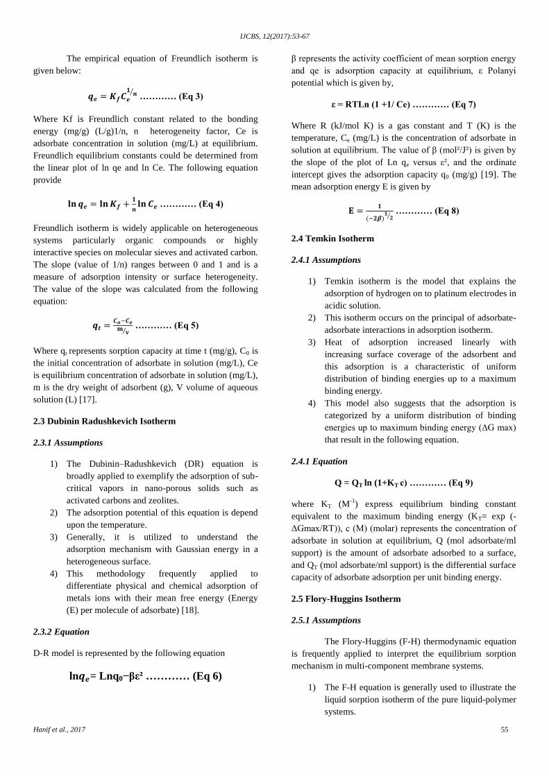
The empirical equation of Freundlich isotherm is
given below:
………… (Eq 3)
Where Kf is Freundlich constant related to the bonding
energy (mg/g) (L/g)1/n, n heterogeneity factor, Ce is
adsorbate concentration in solution (mg/L) at equilibrium.
Freundlich equilibrium constants could be determined from
the linear plot of ln qe and ln Ce. The following equation
provide
………… (Eq 4)
Freundlich isotherm is widely applicable on heterogeneous
systems particularly organic compounds or highly
interactive species on molecular sieves and activated carbon.
The slope (value of 1/n) ranges between 0 and 1 and is a
measure of adsorption intensity or surface heterogeneity.
The value of the slope was calculated from the following
equation:
………… (Eq 5)
Where qt represents sorption capacity at time t (mg/g), C0 is
the initial concentration of adsorbate in solution (mg/L), Ce
is equilibrium concentration of adsorbate in solution (mg/L),
m is the dry weight of adsorbent (g), V volume of aqueous
solution (L) [17].
2.3 Dubinin Radushkevich Isotherm
2.3.1 Assumptions
1) The Dubinin–Radushkevich (DR) equation is
broadly applied to exemplify the adsorption of sub-
critical vapors in nano-porous solids such as
activated carbons and zeolites.
2) The adsorption potential of this equation is depend
upon the temperature.
3) Generally, it is utilized to understand the
adsorption mechanism with Gaussian energy in a
heterogeneous surface.
4) This methodology frequently applied to
differentiate physical and chemical adsorption of
metals ions with their mean free energy (Energy
(E) per molecule of adsorbate) [18].
2.3.2 Equation
D-R model is represented by the following equation
ln = Lnq0−βε² ………… (Eq 6)
β represents the activity coefficient of mean sorption energy
and qe is adsorption capacity at equilibrium, ε Polanyi
potential which is given by,
ε = RTLn (1 +1/ Ce) ………… (Eq 7)
Where R (kJ/mol K) is a gas constant and T (K) is the
temperature, Ce (mg/L) is the concentration of adsorbate in
solution at equilibrium. The value of β (mol²/J²) is given by
the slope of the plot of Ln qe versus ε², and the ordinate
intercept gives the adsorption capacity q0 (mg/g) [19]. The
mean adsorption energy E is given by
………… (Eq 8)
2.4 Temkin Isotherm
2.4.1 Assumptions
1) Temkin isotherm is the model that explains the
adsorption of hydrogen on to platinum electrodes in
acidic solution.
2) This isotherm occurs on the principal of adsorbate-
adsorbate interactions in adsorption isotherm.
3) Heat of adsorption increased linearly with
increasing surface coverage of the adsorbent and
this adsorption is a characteristic of uniform
distribution of binding energies up to a maximum
binding energy.
4) This model also suggests that the adsorption is
categorized by a uniform distribution of binding
energies up to maximum binding energy (ΔG max)
that result in the following equation.
2.4.1 Equation
Q = QT ln (1+KT c) ………… (Eq 9)
where KT (M-1
) express equilibrium binding constant
equivalent to the maximum binding energy (KT= exp (-
ΔGmax/RT)), c (M) (molar) represents the concentration of
adsorbate in solution at equilibrium, Q (mol adsorbate/ml
support) is the amount of adsorbate adsorbed to a surface,
and QT (mol adsorbate/ml support) is the differential surface
capacity of adsorbate adsorption per unit binding energy.
2.5 Flory-Huggins Isotherm
2.5.1 Assumptions
The Flory-Huggins (F-H) thermodynamic equation
is frequently applied to interpret the equilibrium sorption
mechanism in multi-component membrane systems.
1) The F-H equation is generally used to illustrate the
liquid sorption isotherm of the pure liquid-polymer
systems.

IJCBS, 12(2017):53-67
Hanif et al., 2017 56
2) Independence of lattice constants on composition
(artificial).
3) Polymer molecules are of same size.
4) Mean concentration of polymer segments in cells
adjacent to cells unoccupied by the polymeric
solute is equal to the overall average concentration.
5) No effect of mixing on volume change (while in
some favorable interactions between solvent
molecules and polymers may have negative impact
on volume change).
6) There are no energetically preferred arrangements
of polymer segments and solvent molecules in the
solution.
2.5.1 Equation
ΔGmix=RT ni ln φi + nM ln φM +χiM ni φM ............ (Eq 10)
Where ΔHmix represents the enthalpy change of
mixing and ΔSmix represents the mixing entropy. The
subscripts i and M represent the liquid component and
membrane respectively. Φ is the volume fraction, R is the
gas constant, T is the absolute temperature, ni is the number
of moles of component i, and χiM are the F-H interaction
parameters between the liquid and the membrane [20].
2.6 Hill Isotherm
2.6.1 Assumptions
1) Hill Isotherm explains the binding phenomenon of
several species on to a homogeneous surface.
2) According to this model “adsorption is a process in
which ligand binding ability at one site of the
macromolecule, may affect the different binding
sites of the same macromolecule [21].
2.6.2 Equation
………… (Eq 11)
Where, KD, nH, and qH are constants, qe is the amount of
adsorbed solute per weight of adsorbent at equilibrium, Ce
is the concentration of adsorbate at equilibrium.
2.7 Redlich Peterson Isotherm
2.7.1 Assumptions
1) This isotherm is a hybrid form of the Langmuir and
Freundlich isotherms.
2) This model is applicable when concentration in
numerator is linearly dependent and an exponential
function in the denominator exists, but the
adsorption mechanism is in hybrid state and does
not fulfill the ideal condition of monolayer
adsorption when high concentrations are presents
in the liquid.
3) Redlich Peterson isotherm can easily be applied in
both homogeneous and heterogeneous surfaces.
4) If high concentrations are present in liquid then
Freundlich isotherm model is applicable due to the
exponent β tends to zero factor and incase the
condition of lower concentration in liquid is fulfill
then Langmuir isotherm is applied as the β values
are always close to one.
2.7.2 Equation
………… ( Eq 12)
In this equation, KR is the Redlich–Peterson isotherm
constant (Lg-1
), aR is also Redlich-Peterson constant having
a constant unit (Lmg-1
), β is an exponent ranges between 0
and 1. Ce is the equilibrium liquid-phase concentration of
the adsorbate (mgL-1
) and qe is the equilibrium adsorbate
loading onto the adsorbent (mgg-1
) [13].
2.8 Sips Isotherm (Langmuir-Freundlich)
2.8.1 Assumptions
1) Sips isotherm is a combined form of Freundlich
and Langmuir isotherms.
2) It describes an expression that demonstrates a finite
limit of gas relatively at high pressure.
3) It is used to predict the adsorption systems on
heterogeneous surface.
4) At lower concentrations of adsorbate, it illustrates
the conditions of Freundlich isotherm, but at high
concentrations fulfills the conditions of monolayer
adsorption which is the characteristic of the
Langmuir isotherm. Thus, sometimes it is also
called as Langmuir-Freundlich isotherm.
2.8.2 Equation
The Sips isotherm expression for liquid phase is given
below:
………… (Eq 13)
Here, qe represents the adsorbed amount at equilibrium (mg
g-1
), adsorbate concentration is expressed as Ce (mgL-1
) at
equilibrium, Sips maximum adsorption capacity is expressed
as qms (mg g-1
), KS is the Sips equilibrium constant (L mg-1
)m
and Sips model exponent is represented as mS [22].
2.9 Toth Isotherm
2.9.1 Assumptions
1) Though it was initially suggested for monolayer
adsorption to improve Langmuir isotherm fittings
and experimental data. It is also very helpful in
providing valuable suggestions about
heterogeneous adsorption systems satisfying both

IJCBS, 12(2017):53-67
Hanif et al., 2017 57
conditions of low and high concentrations of
adsorbate in liquid system.
2) Both conditions of limits of the isotherm are
satisfied in Toth’s equation.
at p → 0 and p → ∞
Hence it is preferred over Sips isotherm equation [23].
2.9.2 Equation
………… (Eq 14)
In this equation, adsorbed amount is represented by qe (mg
g-1
) at equilibrium, adsorbate concentration at equilibrium is
expressed by Ce (mgL-1
), Toth maximum adsorption
capacity is denoted by qmT (mg g-1
), KT is Toth equilibrium
constant and mT is the Toth model exponent [22].
2.10 Koble Corrigan Isotherm
2.10.1 Assumptions
Basically, Koble–Corrigan isotherm is a three
parameter equation that comprised of both Freundlich and
Langmuir isotherm models that represent adsorption data at
equilibrium stage. The values of isotherm constants A, B
and n are calculated by drawing linear plot with a trial and
error method [23].
2.10.2 Equation
Mathematical equation of Koble–Corrigan
isotherm model can be presented as follows:
………… (Eq 15)
In this expression, qe (mg/g)represents the concentration of
adsorbate in adsorbent at equilibrium Koble-Corrigan
isotherm constant is represented by A (Ln mg1-n/g),is B (L
mg)n is also Koble-Corrigan isotherm constant, n is
adsorption intensity, concentration is represented by Ce
(mg/L) at equilibrium [13].
2.11 Khan Isotherm
2.11.1 Assumptions
It is a general model proposed for the pure
solutions having ak and bk are used to represent model
exponent and model constant respectively. Chi-square
values or minimum ERRSQ (the sum of the squares of the
errors) and values of high correlation coefficients can play
pivotal role in determining maximum removal efficiency/
uptake values of the system [13].
2.11.2 Equation
Mathematical expression of Khan Isotherm model
is given below:
………… (Eq 16)
Here, qe (mg/g)is the amount of adsorbate in adsorbent at
equilibrium, qs (mg/g) is the theoretical isotherm saturation
capacity, concentration is denoted by Ce (mg/L) at
equilibrium, Khan isotherm model exponent is represented
by aK khan isotherm model constant is represented by bK.
2.12 Radke–Prausnitz Isotherm
2.12.1 Assumptions
The correlation in Radke–Prausnitz isotherm model
is commonly figured out by the high root-mean-square error
(RMSE) and chi-square values. Radke–Prausnitz model
exponent is characterized by βR and aR and rR are denoted
as model constants [13].
2.12.2 Equation
Mathematical expression of Radke –Prausnitz
Isotherm is given below:
………… (Eq 17)
In this expression, qe (mg/g) expressed the amount of
adsorbate in adsorbent at equilibrium, arp and rR are
denoted as Radke-Prausnitz isotherm model constants and
βR is Radke-Prausnitz isotherm model exponent.
2.13 Brunauer–Emmett–Teller (BET) Isotherm
2.13.1 Assumptions
Brunauer–Emmett–Teller (BET) isotherm is a
theoretical equation which is normally applicable in gas –
solid adsorption equilibrium system. This theory aims to
develop a multilayer adsorption system under the force of
pressure from 0.05 to 0.30 that result in a monolayer
coverage lying between 0.50 and 1.50.
1) This theory based on the concept of Langmuir
theory that focused on adsorption of a molecule to
a single or multilayer surface with the following
postulates: (a) a molecule of a gas physically
adsorbed to a solid surface infinitely; (b) no
interaction occurs between each adsorption layer;
(c) Langmuir theory is applicable to each layer and
the process of adsorption only occurs on particular
or well defines surface of the sample.
2) When the interaction occurs between the molecules
each molecule provides/ act as a single adsorption
site to a molecule of the upper layer.
3) Molecules from the upper layer will also in
equilibrium state with the gas phase for example
adsorption and desorption rates will be equal.
4) Desorption of a molecule from a solid surface is a
kinetically limited process and there is also need to
provide heat of desorption.
• These processes are homogeneous in nature e.g. a
specific heat or energy is required for adsorption to a given
or particular molecular layer.

IJCBS, 12(2017):53-67
Hanif et al., 2017 58
• E1 represents the energy of the 1st layer, i.e. heat of
adsorption of adsorbate at the surface of the solid sample.
• Other layers are considered as similar and can be
expressed as condensed species (liquid state). Thus, heat of
adsorption EL is equal to the heat of liquefaction.
• Molecular layer numbers tends to infinity
(equivalent to the sample being surrounded by a liquid
phase), at saturation pressure.
2.13.2 Equation
Expression of BET isotherm model is given below:
………… (Eq 18)
In this equation, qe (mg/g) is amount of adsorbate in
adsorbent at equilibrium, qs (mg/g) is theoretical isotherm
saturation capacity, CBET (L/mg) is adsorption isotherm
relating to the energy of surface interaction, Ce (mg/L) is
concentration at equilibrium, and Cs (mg/L) is the
concentration of adsorbate monolayer saturation.
2.14 Frenkel–Halsey–Hill (FHH) Isotherm Model
2.14.1 Assumptions
This adsorption isotherm defines the mechanism of
multilayer water adsorption assuming that an adsorption
potential gradient based on the distance of the adsorbed
water layer from the surface of the particle [24].
The isotherm is derived by assuming the adsorbate
as a uniform thin layer of liquid on a planar having
homogenous and solid surface, considering the effect of
replacement of the solid by the liquid. A molecule in the
adsorbed layer will act differently in these two situations.
2.14.2 Equation
r
………… (Eq 19)
Where, Ce (mg/L) is the equilibrium concentration, Cs
(mg/L) is the concentration of adsorbate on a monolayer
saturation, d, α and r (m) are the sign of the interlayer
spacing, isotherm constant (JmR/mole) and inverse power of
distance from the surface (about 3), respectively.
2.15 MET Isotherm
2.15.1 Assumptions
MacMillan–Teller (MET) isotherm is an adsorption
model interpreted from the inclusion of surface tension
effects in the BET isotherm [13].
2.15.2 Equation
………… (Eq 20)
Where, qe(mg/g) is amount of adsorbate in adsorbent at
equilibrium, qs (mg/g) is theoretical isotherm saturation
capacity, K is MacMillan-Teller isotherm constant, Cs
(mg/L) is adsorbate monolayer saturation concentration, Ce
(mg/L) is concentration at equilibrium.
3. Kinetic Modeling of Adsorption
3.1 Chemical Kinetics
Chemical kinetics, commonly recognized as
reaction kinetics, is the study of rates of chemical processes.
Chemical kinetics play vital role in determining the effect of
different experimental conditions on the speed of chemical
reaction, yield information about the reaction mechanism,
transition states as well as in developing mathematical
models that describes the physical and chemical
characteristics of a chemical reaction. In 1864, "Cato
Guldberg" and "Peter Waage" were considered as the
pioneer of chemical kinetics by proposing a theory "the law
of mass action". According to this law "the speed of
chemical reaction is directly proportional to the quantity of
the reactants". Chemical kinetics has an important role in the
determination of reaction rates that are also very helpful in
developing rate constants and rate laws. Normally, rate laws
are exists for zero (0) (rate of reaction is not depend on
concentration), 1st and 2nd order reactions. Elementary
reactions follow the law of mass action. The rate laws of
stepwise reactions may also be determined by joining rate
laws of different elementary steps that involve more
complex steps during the reaction process. The rate-
determining steps in a chemical reaction also determine
reaction kinetics in a continuous reaction. In continuous 1st
order reaction, steady states also determine the rate law and
the activation energy of the reaction system also
experimentally calculated by solving the Eyring and
Arrhenius equations. Physical states of the reactants,
concentrations of the reactants, temperature required for the
reaction and the type of catalysts either taking part or not in
the reaction all are regarded as key factors influencing the
reaction rate.
3.2 Rate Equation
The rate equation or rate law of a chemical reaction
is defined as "an equation that interconnects the rate of
reaction with pressure or concentration of reactants with
suitable constants (rate coefficients and partial reaction
orders)". Normally, the expression of rate law is expressed
as power law:
………… (Eq 21)
Where [A] and [B] represents the concentration of the
species A and B, respectively and usually expressed in
moles per liter (molarity, M).

IJCBS, 12(2017):53-67
Hanif et al., 2017 59
Partial reaction order exponents are represented in
the above equation and can be calculated experimentally.
The values of x and y exponents are not equal to the values
of stoichiometric coefficients. Rate constant or rate
coefficient of the reaction is represented by k and the value
of "k" is depend upon the ionic strength, temperature, light
irradiation and the surface area of an adsorbent these factors.
The equation rate of a reaction having multi-step
mechanism can frequently derived theoretically by using
quasi-steady state assumptions from the underlying
elementary reactions, and compared with the experimental
rate equation as a test of the assumed mechanism. The
equations may also involve a fractional order, and may
depend on the concentration of an intermediate species.
The rate equation is a differential equation, and can
be integrated to obtain an integrated rate equation that
interconnects the concentrations of reactants or products
with time.
3.3 Order of Reaction
The order of a reaction regarding a particular
substance like catalyst, reactant or product is defined as the
exponent or index in which the concentration term in the
rate equation is increased. The typical form of a rate
equation is in the following form
r = k [A]x[B]
y ………… (Eq 22)
Where [A] and [B] ... are the concentrations and the reaction
orders (or partial reaction orders) for x and y substance are
represented by A and B respectively. The overall sum of
reaction order is the sum x + y + ....
For example, chemical reaction between mercury
(II) chloride and oxalate ion is given below
………… (Eq 23)
Rate equation for the reaction is as follows:
1 2
………… (Eq 24)
In this equation, reaction order for HgCl2 reactant is 1 and
for oxalate ion is 2 and the overall order of a reaction is
1+2=3. The reaction orders in this equation 1 and 2 differ
from the stoichiometric coefficients i.e. 2 and 1. Reaction
orders are calculated experimentally and may help in
producing knowledge about the reaction mechanism and
determining rate steps involved in a reaction.
Elementary or single-step reactions also have
reaction orders that are equal to the stoichiometric
coefficients of individual reactant. The sum of
stoichiometric coefficients of reactants in a reaction is
always equal to the molecularity of the elementary reaction
Complex or multi-step reactions may or may not have
reaction orders equal to their stoichiometric coefficients.
Generally, orders of reaction are positive integers, but they
may also be negative, zero or fractional for each reactant
taking part in a reaction.
3.4 Factors affecting Reaction Rate
3.4.1 Nature of Reactants
Nature/type and strength of bond between
molecules of the reactants significantly accelerate the rate of
transformation into products. Normally, reaction rate varies,
depending upon the type of elements or substances
participating in a reaction. In acid-base reactions, the
formation of salts or ion exchange occurs rapidly. When the
formation of covalent bond occurs between the molecules or
in the formation of macro molecules the reactions takes
place very slowly.
3.4.2 Physical State of Reactants
Physical states (liquid, solid or gas) of reactant is
also a key factor that alters the rate of reaction of reactants
in chemical reaction. When reactants are in same states i.e.
in aqueous solution, thermal motion of the liquid molecules
brings them to close that result in contact, but, when the
reactants are in distinct phases, the reaction is limited to the
interface between the reactants. Chemical reactions only
occur at their particular areas of intact, for example, in
liquids and gases at the surface of fluid. More fine particles
of liquid or solid reactants have larger areas/unit volume that
result in more contact of reactants with the surface, thus
speed up of chemical reaction. In organic chemistry, water
reactions are exempt from the rule that homogeneous
reactions occurs at faster rate than heterogeneous reactions.
3.4.3 Concentration of Reactants
Reactions are occurs due to the collision of reactant
molecules involved in a chemical reaction. The frequency of
colliding ions or molecules is influenced by concentrations
of reactants. The more packed the molecules of the
reactants are, the more rapidly the molecules collide and
react with each other. Hence, an increase in the amount of
reactants will result in rise in the reaction rate and vice
versa. For example, combustion process takes place more
rapidly in normal amount of oxygen (21%) as compared to
in pure oxygen.
3.4.4 Temperature of Reactants
Typically, temperature has a key influence on the
rate of a chemical reaction. Molecules of reactants at higher
temperature gain more thermal energy. Although, collision
frequency of the vibrating molecule is increased at higher
temperatures, but this alone contributes only a very small
proportion of the energy to increase the rate of reaction.
Moreover, an interesting fact that the amount of reacting
molecule with sufficient amount of energy to react (energy
greater than activation energy: E>Ea) is considerably higher

IJCBS, 12(2017):53-67
Hanif et al., 2017 60
and is illustrated by Maxwell–Boltzmann distribution
energies.
The 'rule of thumb' that the rate of chemical
reactions doubles for every 10 °C temperature rise is a
common misconception. This may have been generalized
from the special case of biological systems, where
temperature coefficient (α) is often between 1.5 and 2.5.
3.4.5 Catalysts
A catalyst is a chemical species which have
capability to start a chemical or biochemical reaction and
also have a potential to alter the rate of chemical reaction
without being a part of resultants in a chemical reaction. The
catalyst accelerates the rate of a reaction by providing a
different reaction mechanism by lowering the activation
energies of the reactants. In autocatalysis, a reaction product
is itself a catalyst for that reaction which leads to positive
feedback. Catalysts speed up the forward and backward rate
of reactions and do not affect the position of the equilibria in
a chemical reaction.
3.4.6 Pressure
Pressure play vital role in defining the rate equation
for gaseous reactions. Generally, it is observed that an
increase in pressure will result in rise the number of
collisions between reactants, thus increasing the rate of
reaction. This is because of the fact that the state of a gas is
directly proportional to the partial pressure inserted to a gas.
Furthermore, the rate coefficient of a system may be
changed due to pressure in a straightforward mass-action
system. The products of different high-temperature gas-
phase and rate coefficients of reaction change, when an inert
gas is added in a solution mixture and this process is
commonly known as fall-off and chemical activation. This
happens when endothermic or exothermic reactions occur at
faster rate than heat transfer, causing the reacting molecules
to have non-thermal energy distributions (non-Boltzmann
distribution). When the pressure of a system is increased the
heat transfer rate between the reacting molecules also
increases and the rest of the system nullifies this effect [25].
3.5 Zero Order Reactions
A reaction in which the rate is dependent upon the
concentration of the reactants is known as zero (0) order
reaction. Increasing the concentration of reacting molecule
does not speed up the rate of reaction (i.e. the amount of
substance taking part in chemical reaction is directly
proportional to time). Zero order reactions are usually
initiated when a particular material or substance is required
to start up a chemical reaction like catalyst or surface
saturated by the reactants. The rate law for a zero order
reaction is
Where r is the reaction rate and k is the reaction rate
coefficient with units of concentration or time.
3.5.1 Assumptions of Zero Order Reactions
Zero order reactions:
1) Occurs in a closed system.
2) No net build-up of intermediates.
3) No other reactions occur in a chemical reaction.
3.5.2 Equation
Keeping in view of above mentioned assumptions,
it can be shown by solving a mass balance equation for the
system:
………… (Eq 25)
If this differential equation is integrated it gives an equation
often called as "integrated zero order rate law".
t = 0 ………… (Eq 26)
Where [A]t represents the concentration of the chemical of
interest at a particular time, and [A]0 represents the initial
concentration.
A reaction is said to be zero order reaction when
the graph of concentration data is plotted or drawn versus
time and a straight line is obtained in as a result. A plot of
[A]t vs. time t gives a straight line with a slope of -k.
The half-life of Aa reaction describes the time
required for a half of the reactant to be depleted. For a zero
order reaction the half-life is given by
0 ………… (Eq 27)
3.6 First Order Reactions
A first order reaction depends on the concentration
of only one reactant (a unimolecular reaction). Other
reactants can be present, but each will be in zero order. The
rate law for a reaction that is first order with respect to a
reactant A is given below
………… (Eq 28)
k is the first order rate constant, which has units of 1/s
The integrated first order rate law is
0 ………… (Eq 29)
A plot of lnA vs. time t gives a straight line with a slope of -
k. The half-life of a first order reaction is depend upon the
initial concentration and is given by
………... (Eq 30)
3.7 Pseudo-First-Order Rate Equation
It is very difficult to measure a second order
reaction rate with presence of two reactants A and B. The
concentration of two reactants needed to be followed
simultaneously that is more difficult to calculate the

IJCBS, 12(2017):53-67
Hanif et al., 2017 61
concentration of reactants as a difference. A solution to the
problem is given by pseudo-first order rate equation.
The concentration of one reactant remains
unchanged when supplied in excess amount. The
concentration can be absorbed within the rate constant,
obtaining a pseudo first order reaction constant, because it
depends on the concentration of only one reactant.
For example if the concentration of [B] remains
constant during a chemical reaction, then:
………… (Eq 31)
Where, k'=k[B]0 (k' or kobs with units s−1
) The Pseudo-first
order reaction is also used to calculate the concentration of
reactants ([B]>>[A] for above said example) so that the
reaction may proceed. When only a small quantity of the
reactant is used it is assumed that the concentration of
reactant must be constant. The value of k' for many
reactions having higher but different concentrations of [B], a
graph of k' versus [B] gives K (generally rate constant for
second order ) as a slope.
Liquid-solid state adsorption phenomenon of
malonic acid and oxalic acid on charcoal surface was firstly
described by Lagergren in 1898 to describe the first order
rate equation [26]. This adsorption describe the adsorption
rate on the basis of adsorption capacity of a system taking
part in a chemical process and can be represent as
1 ………… (Eq 32)
Where: qe and qt (mg/g) are the adsorption capacities at
equilibrium at a specific time (t) respectively. k1 (1 min− 1
) is
the pseudo-first-order rate constant for the kinetic model.
Integrating equation with the boundary conditions of qt=0 to
qt=qe and t =0 to t = t, yields
………… (Eq 33)
This can be rearranged to:
………… (Eq 34)
Where, qe and qt represents the adsorption capacity (mgg-1)
and at time t at equilibrium respectively , k1 (min-1) is the
rate constant of pseudo first order adsorption [27].To
distinguish kinetic equations based on adsorption capacity
from solution concentration, Lagergren’s first order rate
equation has been called pseudo-first-order. In recent years,
it has been widely used to describe the adsorption of
pollutants from wastewater in different fields, such as the
adsorption of methylene blue from aqueous solution by
broad bean peels and the removal of malachite green from
aqueous solutions using oil palm trunk fiber [28].
3.8 Second-Order Rate Equation
A second order reaction depends on the
concentrations of one second order reactant, or two first
order reactants.
Reaction rate for a second order reaction is given by
………… (Eq 35)
Or
………… (Eq 36)
Or
………… (Eq 37)
The integrated second order rate laws are respectively
………… (Eq 38)
Or
………… (Eq 39)
[A]0 and [B]0 must be different to obtain that integrated
equation.
The half-life equation for a second order reaction
dependent on one second order reactant is as follows
………… (Eq 40)
For such a reaction, the half-life progressively doubles as
the concentration of the reactant falls to its half initial value.
By taking the log of both sides, the above
expression is expressed as
………… (Eq 41)
3.9 Pseudo-Second-Order Rate Equation
In 1995, Ho illustrated kinetic adsorption process
for divalent metal ions on peat [29-31]. The chemical
bonding among divalent metal ions and availability of polar
functional groups (ketones, aldehydes, phenolics and acids
are responsible for cation exchange capacity of peat. Peat-
metal reaction may be presented in the following equation
which is the most dominant phenomenon in the adsorption
process of Cu2+
ions onto peat surface.
and
Where: P and HP are active sites on the peat surface.
The base of the above two equations were mainly
the adsorption mechanism may considered as second order
and the rate determining step may be due to chemical
adsorption involving adhesion forces through the exchange
or sharing of electrons between divalent metal ions and peat.
Furthermore, the adsorption follows the Langmuir
equation and the rate of adsorption represented by these
equations is depend upon the amount of metal ions adsorbed

IJCBS, 12(2017):53-67
Hanif et al., 2017 62
on the surface of peat at time (t) at equilibrium [32]. Hence,
the rate expression may be expressed as
2 ………… (Eq 43)
Where qe (mg g-1
) and qt are the sorption capacity at
equilibrium at time t, respectively and k (g mg-1
min-1
)
represents the rate constant of pseudo-second order sorption.
The driving force, (qe−qt), is proportional to the available
fraction of active sites. Then, it yields
………… (Eq 44)
Integrating equation with the boundary conditions of qt=0 at
t=0 and qt=qt at t=t yields
………… (Eq 45)
3.10 Third Order Reaction
Third order reaction is said to be a third order if the
rate of reaction is determined by the variation of the
concentration of three species taking part in a reaction. In
simple form, there is need at least three molecules to start a
chemical reaction.
Normally, in chemical reactions, the kinetic
behavior of the reaction is calculated by taking the constants
of the steps having lower rate constant, known as rate
limiting step or rate determining step. Some trimolecular
reactions shows 3rd order kinetics with the following
expression
Where: k is a constant of third order reaction. Three
dimensional collision between the molecules is not a
necessary condition for a third order reaction Alternatively, ,
it was assumed that two-step mechanism is involved but the
first step is occurring reversibly at a faster rate thus, the
concentration of X is given by x = Kab, where, K is the
equilibrium constant for binding of A to B, the association
constant of X. The rate of reaction is then the rate of the
slow second step:
………… (Eq 47)
Where: k' is the rate constant of second-order for second
step in a chemical reaction. Hence the observed third-order
rate constant is actually the product of a second-order rate
constant and equilibrium constant.
A number of reactions are found to have third order
kinetics. An example is the oxidation of NO, for which the
overall reaction equation and rate law are given below.
2NO + O2→ 2NO2 ………… (Eq 48)
………… (Eq 49)
One possibility for the mechanism of this reaction
would be a three-body collision (i.e. a true tri molecular
reaction). However, such collisions are extremely rare. The
rate of this reaction is found to decrease with increasing
temperature, thus, indicating that complex mechanisms are
occurring. Alternative mechanism which leads to the same
rate law is a two-step process involving a pre-equilibrium.
………… (Eq 50)
………… (Eq 51)
The overall rate is
………… (Eq 52)
However, from the pre-equilibrium, we have
So
………… (Eq 53)
and the overall rate is
………… (Eq 54)
i.e third order as required.
3.11 Fractional Order
In fractional order reactions, the order is a non-
integer, which often indicates a chemical chain reaction or
other complex reaction mechanism. For example, the
pyrolysis of ethanal (CH3-CHO) into carbon monoxide and
methane proceeds with an order of 1.5 with respect to
ethanal: r = k[CH3-CHO]3/2
. The breakdown of phosgene
(COCl2) to chlorine and carbon monoxide has order 1 with
respect to phosgene itself and order 0.5 with respect to
chlorine: r = k[COCl2] [Cl2]1/2
.
The order of a chain reaction can be rationalized by
using the steady state calculations for the concentration of
reactive intermediates such as free radicals. For the
pyrolysis of ethanal, the Rice-Herzfeld mechanism is
Initiation
CH3CHO → •CH3 +
•CHO ………… (Eq 55)
Propagation
•CH3 + CH3CHO → CH3CO
• + CH4 ………… (Eq 56)
CH3CO• →
•CH3 + CO ………… (Eq 57)
Termination

IJCBS, 12(2017):53-67
Hanif et al., 2017 63
2 •CH3 → C2H6 ………… (Eq 58)
Where • denotes a free radical. To simplify the theory, the
reactions of the •CHO to form a second
•CH3 are ignored.
In the steady state, formation and destruction rates
of methyl radicals are equal, thus, the concentration of
methyl radicals satisfy
• =0 ………… (Eq 59)
[•
………… (Eq 60)
The reaction rate equals to the rate of the propagation step
which produces the main reaction products CH4 and CO in
agreement with the experimental order of 3/2.
[
•
………… (Eq 61)
3.12 Mixed Order
Different complex rate laws have been used for
studying mixed order reactions; they are applicable to the
laws for more than one order at different concentrations of
the chemical species involved in a chemical reaction. For
example, a rate law of the form r = k1[A]+k2[A]2
represents
concurrent first order and second order reactions (or more
often concurrent pseudo-first order and second order)
reactions, and can be defined as mixed first and second
order. For sufficiently large values of [A] such reactions will
considered as second order kinetics, but for smaller [A] the
kinetics will assumed as first order (or pseudo-first order).
As the reaction progresses, the reaction can change from
second order to first order as reactant is consumed.
Another type of mixed-order rate law has a
denominator of two or more terms, often because the
identity of the rate-determining step depends on the values
of concentrations. An example is the oxidation of an alcohol
to a ketone by hexacyanoferrate (III) ion [Fe(CN)6-3
] with
ruthenate (VI) ion (RuO4-2
) as catalyst.
For this reaction, the rate of disappearance of
hexacyanoferrate (III) is
………… (Eq 62)
This is zero-order with respect to hexacyanoferrate (III) at
the onset of the reaction (when its concentration is high and
the ruthenium catalyst is quickly regenerated), but changes
to first-order when its concentration decreases and the
regeneration of catalyst becomes rate-determining step.
Notable mechanisms with mixed-order rate laws
with two-term denominators include:
1) Michaelis-Menten kinetics for enzyme-catalysis:
first-order in substrate (second-order overall) at
low substrate concentrations, zero order in
substrate (first-order overall) at higher substrate
concentrations
2) Lindemann mechanism for unimolecular reactions:
second-order at low pressures, first-order at high
pressures.
3.13 Negative Order
Rate of a chemical reaction may have a negative
partial order with respect to a substance. For example the
conversion of ozone (O3) to oxygen follows the rate
equation in an excess of oxygen. This corresponds to second
order in ozone and order (-1) with respect to oxygen.
………… (Eq 63)
When a partial order is negative, the overall order is usually
considered as undefined. In the above example for instance,
the reaction is not described as first order even though the
sum of the partial orders is 2 + (-1) = 1, because the rate
equation is more complex than that of a simple first-order
reaction.
3.14 Elovich’s Equation
A kinetic equation of chemisorption was
established by Zeldowitsch in 1934 [33]. It was used to
define and calculate the adsorption rate of carbon monoxide
on manganese dioxide which decreases exponentially with
increasing the concentration of adsorbed gas commonly
called as Elovich equation. The expression for Elovich
equation is as follows [34].
ae
-αq ………… (Eq 64)
Where q represents the amount of gas adsorbed at time t, a is
the desorption constant, and the initial adsorption rate is
expressed as α [35]. The linear expression of the above
equation is given as
………… (Eq 65)
With
………… (Eq 66)
The plot of q versus log (t+t0) provides a straight line with
an opposite value of t0. Elovich equation is applied to
determine the kinetics of chemisorption of gases onto
heterogeneous solidswith the assumption of aαt>>1 [36].
Equation was integrated by using the boundary conditions of
q=0 at t=0 and q=q at t=t to yield

IJCBS, 12(2017):53-67
Hanif et al., 2017 64
………… (Eq 67)
Elovich’s equation has been widely applied to estimate the
amount of a gas adsorbed to a solid surface [28]. Recently, it
has also been widely applied in wastewater treatment
process for the adsorption of toxic pollutants on a solid
surface in aqueous solutions, for example, removal of
Cd(II), Cu(II) and Cr(VI) by using bone char [37], rhizopus
arrhizus and chitin, chitosan respectively in aqueous
solutions [28] removal from effluents using bone char [37]
and Cr(VI) and Cu(II) adsorption by chitin, chitosan, and
Rhizopus arrhizus [28].
4. Thermodynamic Modeling of Adsorption
4.1 Thermodynamics
The term thermodynamics derived from the Greek
word and is a combination of therme (heat) and dynamic
(power). It is a science of energy that deals with the
molecular motion with respect to time. Thermodynamics is
also known as “macroscopic science” which provides
information about the average changes taking place among
larger numbers of molecules Thermodynamics first emerged
as a science after the construction and operation of steam
engines by Thomas Savery and Thomas Newcomen in 1697
and 1712 respectively. Later on, Rankine, Carnot, Kelvin,
Clausius, Gibbs and many others have developed
thermodynamic principles for by describing the laws of
conversion and conservation of energy in a system. The
theoretical equations of classical thermodynamics are a set
of natural laws providing information about the behavior of
macroscopic systems. These laws lead to a large number of
equations, entirely based entirely on logics, and attached to
well-defined constraints in a reaction. Natural conditions
and natural phenomenon are far from adiabatic, reversible,
equilibrium, isothermal or ideal laws, thus, the engineers
exercise these pragmatic approaches in applying the
principles of thermodynamics to real systems. Some other
new attempt has been made to present thermodynamic
principles and there is need to understand and apply these
principles of thermodynamics in modeling, designing, and
describing some natural and complex phenomena. All
disciplines of science and engineering have followed the
applications of thermodynamics. Thermodynamics
principles may also presents methods and “generalized
correlations” for the calculation of physical and chemical
properties of a substance, when there is no experimental
data exists. Such estimations are often necessary in
simulation and designing of various processes.
Thermodynamic is an ideal and model system that
represents a real system describing the theoretical
thermodynamics approach. A simple system is a single state
system with no internal boundaries, and is not subject to
external force fields or inertial forces. The boundary of the
volume separates the system from its surroundings. A
system may be taken through a complete cycle of states, in
which its final state is the same as its original state. In a
closed system, a material content is fixed and an internal
mass changes only due to a chemical reaction. Closed
systems exchange energy only in the form of heat or work
with their surroundings. Material and energy contents are
variable in an open system, and the systems freely exchange
mass and energy with their surroundings. Isolated systems
cannot exchange their matter and energy. A system
surrounded by an insulating boundary is called a thermally
insulated system. The features of a system are based on the
behavior of molecules that related to microscopic state,
which is the key concern of statistical in thermodynamics. In
contrast, classical thermodynamics formulates the
macroscopic states, which describe the average behavior of
large groups of molecules having macroscopic properties
e.g. pressure and temperature. The macroscopic state of a
system can be fully specified by a small number of
parameters, such as the temperature, volume and number of
moles.
4.2 Thermodynamic Properties
Thermodynamic macroscopic attributes of a system
are derived from the long time average of the observable
microscopic coordinates of motion by statistically. For
example, the pressure is an average measure over about
1024 molecule-wall collisions per second per square
centimeter of a surface for a gas at standard conditions.
Thermodynamic is a property of state function and it
depends only on the properties of the initial and final
conditions of the system. The infinitesimal change of a state
function is an exact differential. Properties like mass m and
volume V are defined by the system as a whole. Such
properties are additive, and called as extensive properties.
Separation of the total change for a species into the external
and internal parts may be categorized to any extensive
property. All extensive properties are homogeneous
functions of the first order in the mass of the system. For
example, doubling the mass of a system at constant
composition doubles the internal energy. The pressure P and
temperature T defines the values at each point of the system
and are therefore called intensive properties. Some features
of a system can be expressed as derivatives of extensive
properties, such as temperature.
………… (Eq 68)
Where U is the energy and S is the entropy.
4.3 Energy
Energy is a conserved and extensive property of
every system in any state, and hence its value depends only

IJCBS, 12(2017):53-67
Hanif et al., 2017 65
on the state. Energy is transferred in the forms of heat or
work through the boundary of a system. In a complete cycle
of steady state process, internal energy change is zero and
hence the work done on the system is converted to heat
(work=heat) by the system. The mechanical work of
expansion or compression proceeds with the observable
motion of the coordinates of the particles of matter.
Chemical work, on the other hand, proceeds with changes in
internal energy due to changes in the chemical composition
(mass action).
4.4 Gibbs Free Energy
In thermodynamics, the Gibbs free energy (Gibbs
energy or Gibbs function; also known as free enthalpy)
refers to a thermodynamic potential that measures the
"efficacy" or process-initiating work obtained from a
thermodynamic system at a constant temperature and
pressure (isothermal, isobaric). The Gibbs free energy
(kJ/mol) is the maximum amount of non-expansion work
that can be extracted from a thermodynamically closed
system (one that can exchange heat and work with its
surroundings, but not matter)the maximum form of energy
can be achieved only in a completely reversible process.
When a system undergo in a change from a well-defined
initial state to a well-defined final state, a change in the
expression of Gibbs free energy (ΔP) equals to the amount
of work that has been substituted by a system with its
surroundings, minus the work of the pressure forces, during
a reversible transformation of the system from the initial
state to the final state [38].
4.4.1 Equation
………… (Eq 69)
Which is same as:
………… (Eq 70)
Where:
U is the internal energy (joule), P is pressure
(Pascal), V is volume (m3), T is the temperature (kelvin), S
is the entropy of a system (joule per kelvin), H is the
enthalpy (joule) [39].
4.5 Helmholtz Free Energy
In thermodynamics, the Helmholtz free energy is a
thermodynamic potential that measures the “useful” form of
a work obtained from a closed thermodynamic system at a
constant temperature. The negative difference in the
Helmholtz energy is equal to the maximum amount of work
that the system can perform in a thermodynamic process at
constant temperature. If the volume of a system is changed,
the part of this work done will be performed as boundary
work. The Helmholtz energy is commonly used for systems
held at constant volume. Since in this scenario, no work is
done on the environment, the drop in the Helmholtz energy
is equal to the maximum amount of useful work that can be
extracted from the system. For a system at constant
temperature and volume, the Helmholtz energy will be the
minimum at equilibrium.
4.5.1 Equation
………… (Eq 71)
Where, A is the Helmholtz free energy (joules, CGS: ergs),
U is the internal energy of the system (joules, CGS: ergs), T
is the absolute temperature (kelvins), S is the entropy (joules
per kelvin, CGS: ergs per kelvin).
The Helmholtz energy is the Legendre transform of
the internal energy, U, in which temperature replaces
entropy as the independent variable [40].
4.6 Entropy
In thermodynamics, entropy (usual symbol S) is the
measure of the number of specific ways in which a
thermodynamic system may be arranged, commonly
understood as a measure of disorder. According to the
second law of thermodynamics the entropy of an isolated
system will never decrease and a system will spontaneously
proceed towards its thermodynamic equilibrium configuring
with maximum entropy. Since entropy is a state function,
the change in the entropy of a system is the same for any
process that goes from a given initial state to a given final
state, whether the process is reversible or irreversible.
However, irreversible processes increase the combined
entropy of the system and its surrounding environment.
4.6.1 Equation
………… (Eq 72)
Where: T is the absolute temperature of the system, dividing
an incremental reversible transfer rate of heat into that
system (dQ). (If heat is transferred out the sign would be
reversed giving a decrease in entropy of the system).
Entropy is an extensive property and has a dimension of
energy divided by temperature, which is a unit of joules per
kelvin (J K−1
) in the International System of Units (or kg m2
s−2
K−1
in terms of base units). The entropy of a pure
substance is generally given as an intensive property - either
entropy per unit mass (J K−1
kg−1
) or entropy per unit
amount of substance (J K−1
mol−1
).
5. Conclusion
Adsorption has been recognized as an effective
technology in which solute particles are detached or
IJCBS, 12(2017):53-67
Hanif et al., 2017 66
separated from a liquid through surface interaction with a
solid adsorbent capable of special affinity to a particular
solute particle. Adsorbents used in adsorption mechanism
have different benefits and preferred due to their less
expensive operational cost, easy availability of the sorbent
material, reduced the volume of sludge generated from
industries and the reuse of the adsorbent after the adsorption
process.
Adsorption isotherms are associates with the
amount of adsorbate adsorbed or accumulate per unit weight
of the adsorbent and the concentration of adsorbate in the
solution at a given temperature and equilibrium conditions.
So far, extensive research efforts have been devoted in
building a sound understanding of adsorption isotherm,
kinetics and thermodynamics models that will helpful in
understanding the real time applications of low cost
adsorption materials for the treatment of contaminated
wastewater. In comparison to adsorption isotherm and
kinetics, there is a lack between theoretical and
experimental values of sorption data and disability of the
model to interpret the results.
Over 95% of the experiments have applied linear
models to explain their results related to adsorption data and
hence it is a promising method [13].Thus, there is need to
develop both isotherm and kinetic models in different
adsorption systems in a real field experiment.
References
[1] P. Sampranpiboon, P. Charnkeitkong, X.S. Feng In
Determination of Thermodynamic Parameters of
Zinc (II) Adsorpton on Pulp Waste as Biosorbent,
Advanced Materials Research, 2014; Trans Tech
Publ: 2014; pp 215-219.
[2] A.S. Thajeel. (2013). Isotherm, Kinetic and
Thermodynamic of Adsorption of Heavy Metal
Ions onto Local Activated Carbon. Aquatic Science
and Technology. 1(2): 53-77.
[3] H. Freundlich. (1906). Over the adsorption in
solution. J. Phys. Chem. 57(385471): 1100-1107.
[4] I. Langmuir. (1916). The constitution and
fundamental properties of solids and liquids. Part I.
Solids. Journal of the American chemical society.
38(11): 2221-2295.
[5] O. Redlich, D.L. Peterson. (1959). A useful
adsorption isotherm. Journal of Physical
Chemistry. 63(6): 1024-1024.
[6] S. Brunauer, P.H. Emmett, E. Teller. (1938).
Adsorption of gases in multimolecular layers.
Journal of the American chemical society. 60(2):
309-319.
[7] M. Temkin, V. Pyzhev. (1940). Kinetics of
ammonia synthesis on promoted iron catalysts.
Acta physiochim. URSS. 12(3): 217-222.
[8] R. Sips. (1948). Combined form of Langmuir and
Freundlich equations. J. Chem. Phys. 16(429):
490-495.
[9] A.R. Khan, I. Al-Waheab, A. Al-Haddad. (1996).
A generalized equation for adsorption isotherms for
multi-component organic pollutants in dilute
aqueous solution. Environmental technology.
17(1): 13-23.
[10] R.A. Koble, T.E. Corrigan. (1952). Adsorption
isotherms for pure hydrocarbons. Industrial &
Engineering Chemistry. 44(2): 383-387.
[11] B. Ateya, B. El-Anadouli, F. El-Nizamy. (1984).
The adsorption of thiourea on mild steel. Corrosion
Science. 24(6): 509-515.
[12] A.V. Hill. (1910). The possible effects of the
aggregation of the molecules of haemoglobin on its
dissociation curves. J Physiol (Lond). 40: 4-7.
[13] K. Foo, B.H. Hameed. (2010). Insights into the
modeling of adsorption isotherm systems.
Chemical Engineering Journal. 156(1): 2-10.
[14] X. Chen. (2015). Modeling of experimental
adsorption isotherm data. Information. 6(1): 14-22.
[15] V. Srihari, A. Das. (2008). The kinetic and
thermodynamic studies of phenol-sorption onto
three agro-based carbons. Desalination. 225(1-3):
220-234.
[16] Y. Safa, H.N. Bhatti. (2011). Kinetic and
thermodynamic modeling for the removal of Direct
Red-31 and Direct Orange-26 dyes from aqueous
solutions by rice husk. Desalination. 272(1): 313-
322.
[17] M. Matouq, N. Jildeh, M. Qtaishat, M. Hindiyeh,
M.Q. Al Syouf. (2015). The adsorption kinetics and
modeling for heavy metals removal from
wastewater by Moringa pods. Journal of
Environmental Chemical Engineering. 3(2): 775-
784.
[18] C. Nguyen, D. Do. (2001). The Dubinin–
Radushkevich equation and the underlying
microscopic adsorption description. Carbon. 39(9):
1327-1336.
[19] S.N. Milmile, J.V. Pande, S. Karmakar, A.
Bansiwal, T. Chakrabarti, R.B. Biniwale. (2011).
Equilibrium isotherm and kinetic modeling of the
adsorption of nitrates by anion exchange Indion
NSSR resin. Desalination. 276(1): 38-44.
[20] R.T. Yang. (2013). Gas separation by adsorption
processes. Butterworth-Heinemann: pp.
[21] H. Shahbeig, N. Bagheri, S.A. Ghorbanian, A.
Hallajisani, S. Poorkarimi. (2013). A new
adsorption isotherm model of aqueous solutions on
granular activated carbon. World J. Model. Simul.
9: 243-254.
[22] O. Hamdaoui, E. Naffrechoux. (2007). Modeling of
adsorption isotherms of phenol and chlorophenols

IJCBS, 12(2017):53-67
Hanif et al., 2017 67
onto granular activated carbon: Part II. Models
with more than two parameters. J Hazard Mater.
147(1): 401-411.
[23] S. Tedds, A. Walton, D.P. Broom, D. Book.
(2011). Characterisation of porous hydrogen
storage materials: carbons, zeolites, MOFs and
PIMs. Faraday discussions. 151: 75-94.
[24] C.D. Hatch, A.L. Greenaway, M.J. Christie, J.
Baltrusaitis. (2014). Water adsorption constrained
Frenkel–Halsey–Hill adsorption activation theory:
Montmorillonite and illite. Atmospheric
environment. 87: 26-33.
[25] P. Atkins, J. De Paula. (2013). Elements of
physical chemistry. Oxford University Press, USA:
pp.
[26] S. Lagergren. (1898). About the theory of so-called
adsorption of soluble substances.
[27] E. Abechi, C. Gimba, A. Uzairu, J. Kagbu. (2011).
Kinetics of adsorption of methylene blue onto
activated carbon prepared from palm kernel shell.
Arch Appl Sci Res. 3(1): 154-164.
[28] H. Qiu, L. Lv, B.-c. Pan, Q.-j. Zhang, W.-m.
Zhang, Q.-x. Zhang. (2009). Critical review in
adsorption kinetic models. Journal of Zhejiang
University-Science A. 10(5): 716-724.
[29] H. Yuh-Shan. (2004). Citation review of Lagergren
kinetic rate equation on adsorption reactions.
Scientometrics. 59(1): 171-177.
[30] Y.-S. Ho. Absorption of heavy metals from waste
streams by peat. University of Birmingham, 1995.
[31] Y.-S. Ho. (2006). Second-order kinetic model for
the sorption of cadmium onto tree fern: a
comparison of linear and non-linear methods.
Water Research. 40(1): 119-125.
[32] Y.-S. Ho, G. McKay. (2000). The kinetics of
sorption of divalent metal ions onto sphagnum
moss peat. Water Research. 34(3): 735-742.
[33] J. Zeldowitsch. (1934). Adsorption site energy
distribution. Acta phys. chim. URSS. 1: 961-973.
[34] M. Low. (1960). Kinetics of Chemisorption of
Gases on Solids. Chemical Reviews. 60(3): 267-
312.
[35] Y.-S. Ho, G. McKay. (1998). Sorption of dye from
aqueous solution by peat. Chemical Engineering
Journal. 70(2): 115-124.
[36] S. Chien, W. Clayton. (1980). Application of
Elovich equation to the kinetics of phosphate
release and sorption in soils. Soil Science Society
of America Journal. 44(2): 265-268.
[37] W. Cheung, Y. Szeto, G. McKay. (2007).
Intraparticle diffusion processes during acid dye
adsorption onto chitosan. Bioresource Technology.
98(15): 2897-2904.
[38] W. Greiner, L. Neise, H. Stöcker. (2012).
Thermodynamics and statistical mechanics.
Springer Science & Business Media: pp.
[39] P. Perrot. (1998). A to Z of Thermodynamics.
Oxford University Press on Demand: pp.
[40] A.D. McNaught, A.D. McNaught. (1997).
Compendium of chemical terminology. Blackwell
Science Oxford: pp.