
Cornelia Gießler Theoretical investigations of ... · Abstract The electromagnetic flow control...
113
Cornelia Gießler Theoretical investigations of electromagnetic control of glass melt flow
Transcript of Cornelia Gießler Theoretical investigations of ... · Abstract The electromagnetic flow control...
Cornelia Gießler Theoretical investigations of electromagnetic control of glass melt flow


Theoretical investigations of electromagnetic control of
glass melt flow
Von Cornelia Gießler
Universitätsverlag Ilmenau 2008

Impressum Bibliografische Information der Deutschen Nationalbibliothek Die Deutsche Nationalbibliothek verzeichnet diese Publikation in der Deutschen Nationalbibliografie; detaillierte bibliografische Angaben sind im Internet über http://dnb.d-nb.de abrufbar.
Diese Arbeit hat der Fakultät Maschinenbau als Dissertation vorgelegen Tag der Einreichung: 8. Februar 2008 1. Gutachter: Univ.-Prof. Dr. rer. nat. habil. Andre Thess; Technische Universität Ilmenau 2. Gutachter: Associate Professor Oleg Zikanov,
University of Michigan, Dearborn 3. Gutachter: Dr.-Ing. Ulrich Lange,
SCHOTT AG, Mainz Tag der Verteidigung: 2. Juni 2008
Technische Universität Ilmenau/Universitätsbibliothek Universitätsverlag Ilmenau Postfach 10 05 65 98684 Ilmenau www.tu-ilmenau.de/universitaetsverlag Herstellung und Auslieferung Verlagshaus Monsenstein und Vannerdat OHG Am Hawerkamp 31 48155 Münster www.mv-verlag.de ISBN 978-3-939473-37-4 (Druckausgabe) urn:nbn:de:gbv:ilm1-2008000104
Abstract
The electromagnetic flow control of fluids with high electrical conductivity like liquidmetals has been investigated so far and is well established in industrial processes. Theapplication of electromagnetic (Lorentz) forces in fluids with a low electrical conductivitysuch as glass melts is a comparably new topic. The Lorentz force in glass melts can begenerated by the interaction of an imposed electrical current and an external magneticfield. Basically, the Lorentz force can be used to regulate the mass flow rate in a duct ora pipe or to improve the mixing.
This theoretical work addresses both applications in glass melts and focuses on the con-sideration of the temperature-dependent viscosity and electrical conductivity.
In the first main part of the thesis the pipe flow of glass melt is studied on the basisof an one-dimensional analytical model. The flow is influenced by Lorentz force andgravity as well as temperature variation due to wall heat loss, electrical heating, advection,and heat diffusion. For high and very low driving forces the mean velocity is found tobe proportional to the forces as known from laminar pipe flow with constant materialproperties. In between these two regimes, however, a new flow regime is identified. Ifthere are no heat losses through the wall, the mean velocity is proportional to the squareroot of the driving force. In the presence of wall heat loss the solution for the steadyflow is even found to be non-unique, and to involve bifurcations. This nonlinear behavioris shown to be a result of the closed-loop interaction between the velocity, temperature,and temperature-dependent material properties. The results of the analytical model arevalidated by two-dimensional axisymmetric numerical simulations. The non-unique flowcharacteristic could be observed in a simple non-magnetic experiment.
In the second main part of the thesis three-dimensional numerical simulations of glassmelt in a small scale crucible heated by two rod electrodes are presented. The Lorentzforce leads to an overall increase of the kinetic energy and, if it is the dominating drivingforce, the mean velocity is found to be an almost linear function of the Lorentz force. Thetransition from a buoyancy dominated flow regime to a Lorentz force dominated one andvice versa is characterized by a hysteresis. One obtains two steady solutions for one setof parameters depending on the starting conditions of the steady calculations. The three-dimensional problem is then reduced to an one-dimensional set of algebraic equationsdescribing steady buoyancy driven laminar flow of glass melt in a closed loop under theinfluence of a localized Lorentz force. The loop is a highly simplified representation ofa closed streamline in glass melt flow in the small scale crucible or a real furnace. Themodel reveals the role of temperature-dependent viscosity and conductivity in glass meltflows in a pure form that is not visible in full numerical simulations. Finally, the resultsobtained with the different approaches are compared with each other.
v


Zusammenfassung
Die elektromagnetische Stromungskontrolle von Flussigkeiten mit hoher elektrischer Leit-fahigkeit wird bereits in verschiedenen Bereichen industriell genutzt. Vergleichsweise neuist die Anwendung elektromagnetischer (Lorentz) Krafte zur Beeinflussung von Fluidenmit geringer elektrischer Leitfahigkeit, wie beispielsweise Glasschmelzen. Die Lorentzkraftin Glasschmelzen wird durch die Uberlagerung eines eingepragten elektrischen Stromesund eines externen Magnetfeldes erzeugt. Grundsatzlich kann die Lorentzkraft zur Durch-flussregulierung und fur das Durchmischen genutzt werden. Diese theoretische Arbeit wid-met sich beiden Anwendungsmoglichkeiten unter Berucksichtigung der charakteristischenMaterialeigenschaften von Glasschmelzen.
Im ersten Teil der Dissertation wird die Rohrstromung von Glasschmelzen anhand eineseindimensionalen analytischen Modells untersucht. Die Stromung wird durch Lorentzkraftund Gravitation beeinflusst. Weiterhin werden Temperaturanderungen durch Warme-verluste, direkte elektrische Heizung, Konvektion und Warmeleitung in die Betrachtungeinbezogen. Wie bei laminarer Rohrstromung mit konstanten Materialeigenschaften hangtdie mittlere Geschwindigkeit im Bereich hoher und sehr niedriger antreibender Krafte li-near von diesen ab. Fur reine Heizung wird eine neue laminare Stromungscharakteristikbeobachtet – das Quadrat der mittleren Geschwindigkeit ist proportional zur antreiben-den Kraft. Bei Kuhlung jedoch kann das Stromungsverhalten Bifurkationen – mehr-wertige Losungen – aufweisen, die bereits durch ein einfaches nicht-magnetisches Experi-ment nachgewiesen werden konnen. Dieses nichtlineare Verhalten wird durch die starkeKopplung von Geschwindigkeit, Temperatur und temperaturabhangigen Materialeigen-schaften hervorgerufen. Die Ergebnisse des analytischen Modells werden durch zwei-dimensionale, axialsymmetrische Simulationen validiert.
Im zweiten Teil dieser Arbeit wird dreidimensionale Stromungssimulationen von Glas-schmelze in einem Tiegel prasentiert. Die Lorentzkraft fuhrt insgesamt zu einer Zu-nahme der kinetischen Energie. Die mittlere Geschwindigkeit ist eine lineare Funktion derLorentzkraft, falls diese dominiert. Der Ubergang von einer vorwiegend durch Auftriebangetriebenen Stromung zu einer elektromagnetisch gesteuerten Stromung ist durch eineHysterese gekennzeichnet. Man erhalt zwei verschiedene stationare Stromungsstrukturenfur einen gegebenen Steuerparameter. Die Losung hangt dabei von den Anfangsbedin-gungen der Berechnung ab. Weiterhin kann das dreidimensionale Problem auf eineStromung in einem geschlossenen Rohrkreislauf reduziert werden. Die mittlere Geschwin-digkeit wird dabei durch eine algebraische Gleichung beschrieben. Der geschlosseneRohrkreislauf ist die stark vereinfachte Darstellung einer geschlossenen Stromlinie ineinem Tiegel unter dem Einfluss der Lorentzkraft. Das Modell ermoglicht klar denEinfluss der tempera-turabhangigen Viskositat und elektrischen Leitfahigkeit auf dasStromungsverhalten aufzuzeigen.
vii


Contents
1 Introduction 1
1.1 Electromagnetic forces in glass processing . . . . . . . . . . . . . . . . . . . 11.2 Characteristics of glass melt and glass melt flow . . . . . . . . . . . . . . . 41.3 Flow control of glass melt . . . . . . . . . . . . . . . . . . . . . . . . . . . 61.4 Scope of thesis . . . . . . . . . . . . . . . . . . . . . . . . . . . . . . . . . 9
2 Electromagnetically controlled flow in a pipe 11
2.1 Formulation of the analytical model . . . . . . . . . . . . . . . . . . . . . . 132.2 Solution method . . . . . . . . . . . . . . . . . . . . . . . . . . . . . . . . 162.3 Selected results . . . . . . . . . . . . . . . . . . . . . . . . . . . . . . . . . 17
2.3.1 Heating without wall heat loss . . . . . . . . . . . . . . . . . . . . . 172.3.2 Heating with wall heat loss . . . . . . . . . . . . . . . . . . . . . . . 212.3.3 Influence of diffusion . . . . . . . . . . . . . . . . . . . . . . . . . . 242.3.4 Sample calculations with glass melt parameters . . . . . . . . . . . 25
2.4 Validation by numerical simulation . . . . . . . . . . . . . . . . . . . . . . 272.4.1 Implemented model and method . . . . . . . . . . . . . . . . . . . . 272.4.2 Results . . . . . . . . . . . . . . . . . . . . . . . . . . . . . . . . . . 29
2.5 Simple experimental study of a non-magnetic case . . . . . . . . . . . . . . 332.5.1 Experimental setup and procedure . . . . . . . . . . . . . . . . . . 332.5.2 Results . . . . . . . . . . . . . . . . . . . . . . . . . . . . . . . . . . 36
2.6 Summary and discussion . . . . . . . . . . . . . . . . . . . . . . . . . . . . 37
3 Electromagnetically controlled flow in a crucible 39
3.1 Three-dimensional numerical simulation . . . . . . . . . . . . . . . . . . . 393.1.1 Formulation of the problem . . . . . . . . . . . . . . . . . . . . . . 403.1.2 Implementation and numerical model . . . . . . . . . . . . . . . . . 443.1.3 Results . . . . . . . . . . . . . . . . . . . . . . . . . . . . . . . . . . 45
3.2 One-dimensional analytical model . . . . . . . . . . . . . . . . . . . . . . . 613.2.1 Formulation of the problem . . . . . . . . . . . . . . . . . . . . . . 623.2.2 Results . . . . . . . . . . . . . . . . . . . . . . . . . . . . . . . . . . 67
3.3 Comparison between numerical, analytical, and experimental results . . . . 763.3.1 Adjustment of model parameters and material property laws . . . . 763.3.2 Sample calculations for the analytical model . . . . . . . . . . . . . 783.3.3 Comparison between numerical and analytical results . . . . . . . . 793.3.4 Comparison with experimental data . . . . . . . . . . . . . . . . . . 82
3.4 Summary and discussion . . . . . . . . . . . . . . . . . . . . . . . . . . . . 84
4 Outlook 87
ix

x Contents
Bibliography 89
A Appendix 95
A.1 Averaged momentum and energy equations for non-isothermal pipe flow . . 95A.2 Validation of convective boundary condition . . . . . . . . . . . . . . . . . 96A.3 Estimation of heat transfer coefficient h . . . . . . . . . . . . . . . . . . . . 97A.4 Mesh study . . . . . . . . . . . . . . . . . . . . . . . . . . . . . . . . . . . 98A.5 Material properties . . . . . . . . . . . . . . . . . . . . . . . . . . . . . . . 100

1 Introduction
Everything should be made as simple as possible, but notsimpler.
A. Einstein
Glass is an ubiquitous material whose production is the most ancient form of industryas it can be dated back to 2,500 BC [81]. Nowadays the need of high quality glassproducts still requires permanent improvement of the production process and explorationof new production techniques. Furthermore, a reliable processing of glass melts needs anaccurate flow prediction and reliable flow control mechanism. Electromagnetic forces areone possibility to control the flow of glass melts which is a comparatively new topic forglass manufacturers. For the application it is essential to know,
whether electromagnetic forces can lead to sufficient strong changes in the flow velocityso as to control the mass flow rate, to enhance mixing, and to generate any desired flow
pattern.
The present thesis will answer this question on the basis of analytical models and numer-ical simulations for basic geometries to obtain a deeper understanding of the underlyingphysical mechanism. Moreover, the thesis will study,
how the glass melt material properties influence the electromagnetically driven flow.
In this chapter a brief introduction to the topic shall be given by describing electromag-netic forces in glass melts in Sec. 1.1, followed by an explanation of the characteristics ofmolten glass which are relevant for our considerations in Sec. 1.2. In Sec. 1.3 we brieflyintroduce common processing techniques and discuss possible applications of electromag-netic forces. This chapter concludes with the scope of the thesis in Sec. 1.4.
1.1 Electromagnetic forces in glass processing
While the application of electromagnetic forces for flow control in other areas of materialprocessing like steel casting and production of aluminum is well established [13], theapplication of electromagnetic forces in glass melts is a comparably new topic. Thedifficulty with glass melts arises from the fact that their electrical conductivity is nearlyfive orders of magnitude smaller than that of liquid metals. Electromagnetic forces, alsocalled Lorentz forces f , are generated by the superimposition of an electric current densityJ and a magnetic flux density B according to
f = J × B. (1.1)
1
2 1 Introduction
We distinguish between different types of Lorentz forces as the origin of J and B aremanifold [38].
The electric current density spreads out in electrically conducting media with the electricalconductivity σ > 0 S/m. The different possibilities of the current density generation arecombined in Ohm’s law [52]
J = σ
(−∇φ + u× B− ∂A
∂t
). (1.2)
The first component −σ∇φ results from the gradient of the spatial distributed electricpotential ∇φ. Furthermore, the superimposition of the movement of an electrically con-ducting liquid or solid body with the velocity u and a magnetic field yields an so-calledinduced current density σ(u×B). It is comparably small due to the small velocities andthe low electrical conductivity of molten glass. During the modeling of electric currentdensities in glass melt flow this component is always neglected. Additionally, a time-varying magnetic field leads to a second induced current density component σ(−∂A/∂t)where A is the magnetic vector potential. This induced current is used in glass industryfor cold crucible induction furnaces [39] as the frequency of the magnetic field is high. Aswe consider time-independent magnetic fields in the present work, this induced currentdensity is zero.
The second component of the Lorentz force, the magnetic flux density B with B =∇× A, can be given as an external magnetic field which we label B0. Furthermore, theelectric current is surrounded by a magnetic field according to Ampere’s law ∇×B = µJ.In general, the magnetic field around spatial distributed currents in the glass melt isnegligible whereas the magnetic field around current carrying electrodes BE immersedinto glass melt is comparably large [33].
The first Lorentz force component we like to introduce is based on the magnetic fieldaround an electrode BE and the electric current in the melt
fLn = σ(−∇φ) ×BE. (1.3)
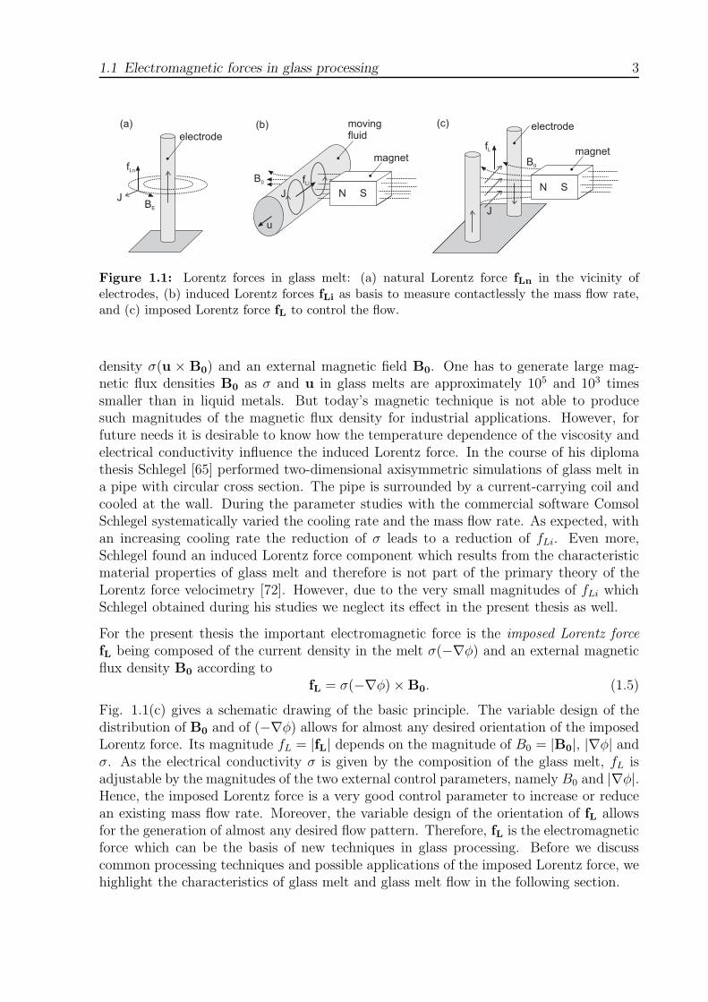
It is called natural Lorentz force and always exists in the vicinity of electrodes. A schematicdiagram of fLn is given in Fig. 1.1(a). There is a long-standing and still unresolved con-troversy ([32], [9], [33]) as to whether naturally occurring electromagnetic forces shouldbe included into models of glass melt flows. Similar flows occur in a variety of electro-magnetic materials processing techniques and are often called electrically induced vorticalflows [3]. We neglect the effects of the natural Lorentz force in our considerations as wefocus on electromagnetic forces in glass melts which can be used to control the flow.
In the future the induced Lorentz force
fLi = σ(u× B0) ×B0 (1.4)
can become interesting for glass manufacturers as it is the basis for the Lorentz forcevelocimetry [73] which is already successfully used for the contactless mass flow measure-ment of liquid metals [40]. As shown in Fig. 1.1(b) it is formed by an induced current
1.1 Electromagnetic forces in glass processing 3
Figure 1.1: Lorentz forces in glass melt: (a) natural Lorentz force fLn in the vicinity ofelectrodes, (b) induced Lorentz forces fLi as basis to measure contactlessly the mass flow rate,and (c) imposed Lorentz force fL to control the flow.
density σ(u × B0) and an external magnetic field B0. One has to generate large mag-netic flux densities B0 as σ and u in glass melts are approximately 105 and 103 timessmaller than in liquid metals. But today’s magnetic technique is not able to producesuch magnitudes of the magnetic flux density for industrial applications. However, forfuture needs it is desirable to know how the temperature dependence of the viscosity andelectrical conductivity influence the induced Lorentz force. In the course of his diplomathesis Schlegel [65] performed two-dimensional axisymmetric simulations of glass melt ina pipe with circular cross section. The pipe is surrounded by a current-carrying coil andcooled at the wall. During the parameter studies with the commercial software ComsolSchlegel systematically varied the cooling rate and the mass flow rate. As expected, withan increasing cooling rate the reduction of σ leads to a reduction of fLi. Even more,Schlegel found an induced Lorentz force component which results from the characteristicmaterial properties of glass melt and therefore is not part of the primary theory of theLorentz force velocimetry [72]. However, due to the very small magnitudes of fLi whichSchlegel obtained during his studies we neglect its effect in the present thesis as well.
For the present thesis the important electromagnetic force is the imposed Lorentz forcefL being composed of the current density in the melt σ(−∇φ) and an external magneticflux density B0 according to
fL = σ(−∇φ) × B0. (1.5)
Fig. 1.1(c) gives a schematic drawing of the basic principle. The variable design of thedistribution of B0 and of (−∇φ) allows for almost any desired orientation of the imposedLorentz force. Its magnitude fL = |fL| depends on the magnitude of B0 = |B0|, |∇φ| andσ. As the electrical conductivity σ is given by the composition of the glass melt, fL isadjustable by the magnitudes of the two external control parameters, namely B0 and |∇φ|.Hence, the imposed Lorentz force is a very good control parameter to increase or reducean existing mass flow rate. Moreover, the variable design of the orientation of fL allowsfor the generation of almost any desired flow pattern. Therefore, fL is the electromagneticforce which can be the basis of new techniques in glass processing. Before we discusscommon processing techniques and possible applications of the imposed Lorentz force, wehighlight the characteristics of glass melt and glass melt flow in the following section.

4 1 Introduction
1.2 Characteristics of glass melt and glass melt flow
Glass melt is assumed to be a Newtonian fluid. It is characterized by a very high dynamicviscosity η and a very low electrical conductivity σ. Like the viscosity of magma andpolymers, η of glass melt decreases nonlinearly with the temperature T . In glass science itis common to express this dependence with the so-called Vogel-Fulcher-Tammann equation[54], which is
η(T ) = η0 exp
(A
T + B
). (1.6)
The constant parameters η0, A, and B depend on the fluid, whereas B is typically negative.Since η → ∞ for T → |B| the viscosity law, Eq. (1.6), only makes sense for T > −B.The viscosity can vary more than one order of magnitude in typical working temperatureranges. In Tabs. A.1, A.2, and Fig. A.3 of the appendix examples can be found on thebasis of three types of glass melts which we have considered in the thesis. Several analyticalmodels describing the flow of magma [55], [30], [87], polymeres [63], and glass melt [48],[23] revealed that the temperature-dependent viscosity modifies the flow significantly. Itcan lead to non-linear flow characteristics, instabilities, and multi-valued solutions evenin simple geometries like channels or pipes.
Like η(T ), the electrical conductivity σ(T ) can vary over one order of magnitude and canalso be approximated by an exponential function, the law of Rasch and Hinrichsen
σ(T ) = σ0 exp
(−E
T
), (1.7)
again with constant parameters σ0, and E specific to the considered glass melt [54]. Incontrast to η(T ), the electrical conductivity is increasing with T . Depending on the com-position of the melt and the temperature range there are typical values for the electricalconductivity ranging from σ = 0.1 S/m up to 10 S/m, which is about 104 to 106 timeslower than σ of liquid metals. The dependence of σ on T is especially of interest for setupswith an electric current distribution and hence, with imposed Lorentz forces fL, as J isproportional to σ(T ) according to Eq. (1.2). Let us note that the electric potential φdepends on σ as well, as it calculates from the Laplace equation
∇ · (−σ(T )∇φ) = 0, (1.8)
which results from the solenoidality of the current density ∇ · J = 0, and J = −σ(∇φ).Additionally, the temperature dependency of σ influences the direct electrical heatingsignificantly where the volumetric heat input is
q = σ(T )(∇φ)2. (1.9)
In an unstable system a perturbation by an increasing temperature leads to an amplifiedσ(T ) and thus to an amplified q. If the heat transport mechanisms in the melt are not ableto remove the increasing heat input, it results in higher temperatures. This self-inducedrunaway of the temperature is also denoted as thermal instability [76]. Previous studieshave shown that mainly systems with pure heat conduction tend to be thermally unstable

1.2 Characteristics of glass melt and glass melt flow 5
whereas internal radiation stabilizes the system [67]. The thermal instability takes placein hot regions, e.g. locally around electrodes of production furnaces, or globally in small-scale crucibles with direct electric heating. If a required processing temperature is in suchan unstable regime, the heat input has to be controlled continuously over the electricpotential [69]. Alternatively, thermal stability can be achieved theoretically by assuminga constant current density J0 as it leads to
q =J2
0
σ(T ). (1.10)
Another characteristic of glass melts is a very large Prandtl number Pr ≫ 1 being definedby
Pr =ηcP
λ, (1.11)
with the heat capacity cP , and the heat conductivity λ. The Prandtl number gives theratio between the viscous and the thermal diffusion. It describes the relative growth of thevelocity and the thermal boundary layer thickness, δs and δt, respectively. For laminar flowover a flat plate the relation Pr1/2 ∼ δs/δt is valid [77]. Hence, for glass melt flow we canexpect that the thermal boundary layer is much smaller than the velocity boundary layer,δt ≪ δs. This characteristic of glass melts is important, e.g. for numerical simulations asthe correct resolution of the extremely small boundary layer requires a study of the mesh.Therefore, the resolution of the boundary layers will be part of the mesh studies whichwe present in the Appendix A.4.
The flow of glass melts can be described as very slow and creeping. Therefore, theassumption of laminar flow is frequently used in the glass community. It is supportedby a low Reynolds number Re < 1 which gives the ratio of inertia and viscous forces inforced convection and is defined by
Re =uLρ
η, (1.12)
with the magnitude of the velocity u = |u|, the density ρ, and a characteristic length L.
However, the classification of the flow regimes for free convection, i.e. laminar, turbulentand the transition from laminar to turbulent, is based on the Rayleigh number Ra. It isthe product of the Grashof and the Prandtl number and defined by
Ra = Gr · Pr =gβ∆TL3ρ2cP
ηλ, (1.13)
with the acceleration of gravity g, the thermal expansion coefficient β, and a characteristictemperature difference ∆T . The transition from a spatially symmetric laminar flow to anasymmetric laminar flow is of particular interest for glass melts. Typically, the Rayleighnumber in glass melt flow can become large which implies that the symmetric laminar flowregime might be left. This symmetry breaking is observed for Ra & 105 in convectioncells with bottom-heated and top-cooled walls (Benard cells) [44], [45], and as well incavities with internal volumetric heat sources [46]. Studies with temperature-dependentviscosity representing the Earth’s mantle convection showed that the transition shifts

6 1 Introduction
to smaller values of Ra if the viscosity contrast within the system increases [56], [53].Lim et al. [49] showed numerically for a container glass in a standard melting furnacewithout direct electrical heating that the flow can become unsteady for a volume-averagedRayleigh number of Ra ∼ 104 and more chaotic for Ra ∼ 106, which occurred for typicallength scales and temperature differences in the production process. It shows, that thefrequently used assumption of symmetric and steady glass melt flow can be left and hasto be controlled carefully.
Altogether, the underlying fluid dynamical problem of the high-Prandtl number fluid withnonlinear temperature-dependent viscosity and electrical conductivity is characterized bylow Reynolds and high Rayleigh numbers.
Let us stress that the large variations of the material properties make it difficult to specifythe exact values of the characteristic non-dimensional numbers. Therefore, frequently thenon-dimensional numbers are given for a reference temperature or for certain values of thematerial properties. Additional characteristic numbers summarize the material propertylaws as suggested by Hrma [34]. In [49] Lim and co-workers used volume-averaged values ofthe non-dimensional numbers. This method will fail most of the time as it does not reflectthe characteristics of the material properties. Alternatively, often just a coarse parameterdomain for the characteristic numbers is given and the input and output parameters for aconsidered system carry SI units. In the present thesis we will introduce non-dimensionaldescriptions for analytical models like in Secs. 2.1 and 3.2 as the number of characteristicnumbers is manageable. The results of the three-dimensional simulations of Sec. 3.1 aregiven in dimensional form due to the complexity of the physical model.
1.3 Flow control of glass melt
The goal of glass processing is to provide a chemical homogeneous melt to satisfy thequality standards which is carefully cooled down to a defined temperature and has acertain mass flow rate at the forming device. Electromagnetic forces are an alternative oran enhancement to already established manufacturing processes for all those requirements.
Most industrial furnaces for glass mass production are featured by continuous manufac-turing processes. The design of such constructions is manifold, see e.g. [54], [76], [74]. Fig.1.2 just pictures a simplified schematic drawing to explain the basics of the process. Typ-ically the solid granular is continuously fed to the surface of the melt. Burners above thesurface apply steady radiative non-uniform heat in horizontal direction which is inducinga thermally driven convection. Alternatively, in the case of electric melting, or in addition,in the case of electric boosting, electrodes are placed in the melt. The volumetric heatinput leads to temperature gradients and buoyancy driven convection which is mixing themelt. The melt flows through a throat from the melting zone to the conditioning zone ofthe furnace in which the temperature homogenization starts. The furnace is connected tothe forming device by a forehearth and a feeder which are usually ducts or pipes. In thesefeeder systems, the glass has to be cooled from the necessary refining temperature downto a suitable forming temperature. This cooling process must be carefully controlled inorder to avoid defects induced by strong temperature gradients such as inhomogeneities
1.3 Flow control of glass melt 7
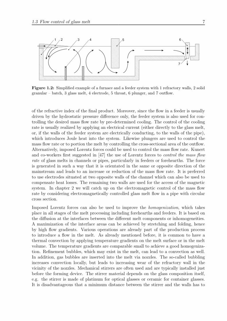
Figure 1.2: Simplified example of a furnace and a feeder system with 1 refractory walls, 2 solidgranular – batch, 3 glass melt, 4 electrode, 5 throat, 6 plunger, and 7 outflow.
of the refractive index of the final product. Moreover, since the flow in a feeder is usuallydriven by the hydrostatic pressure difference only, the feeder system is also used for con-trolling the desired mass flow rate by pre-determined cooling. The control of the coolingrate is usually realized by applying an electrical current (either directly to the glass melt,or, if the walls of the feeder system are electrically conducting, to the walls of the pipe),which introduces Joule heat into the system. Likewise plungers are used to control themass flow rate or to portion the melt by controlling the cross-sectional area of the outflow.Alternatively, imposed Lorentz forces could be used to control the mass flow rate. Kunertand co-workers first suggested in [47] the use of Lorentz forces to control the mass flowrate of glass melts in channels or pipes, particularly in feeders or forehearths. The forceis generated in such a way that it is orientated in the same or opposite direction of themainstream and leads to an increase or reduction of the mass flow rate. It is preferredto use electrodes situated at two opposite walls of the channel which can also be used tocompensate heat losses. The remaining two walls are used for the access of the magneticsystem. In chapter 2 we will catch up on the electromagnetic control of the mass flowrate by considering electromagnetically controlled glass melt flow in a pipe with circularcross section.
Imposed Lorentz forces can also be used to improve the homogenization, which takesplace in all stages of the melt processing including forehearths and feeders. It is based onthe diffusion at the interfaces between the different melt components or inhomogeneities.A maximization of the interface areas can be achieved by stretching and folding, henceby high flow gradients. Various operations are already part of the production processto introduce a flow in the melt. As already mentioned before, it is common to have athermal convection by applying temperature gradients on the melt surface or in the meltvolume. The temperature gradients are comparable small to achieve a good homogeniza-tion. Refinement bubbles, which may exist in the melt, can lead to a convection as well.In addition, gas bubbles are inserted into the melt via nozzles. The so-called bubblingincreases convection locally, but leads to increasing wear of the refractory wall in thevicinity of the nozzles. Mechanical stirrers are often used and are typically installed justbefore the forming device. The stirrer material depends on the glass composition itself,e.g. the stirrer is made of platinum for optical glasses or ceramic for container glasses.It is disadvantageous that a minimum distance between the stirrer and the walls has to
8 1 Introduction
be met to avoid corrosion. Therefore, mechanical stirrers can only influence parts of themelt.
1972 Walkden first patented [82] methods to use the imposed Lorentz force for homog-enization. He suggested different arrangements in feeders and furnaces and recognizedthat the method allows for the production of a variety of different glass flow patterns. Fora feeder system with three electrodes and two magnets a detailed schematic descriptionof the flow pattern with different polarizations of the magnet is given. The patent lacksfurther detailed requirements, e.g. on the dimensions of the setup and on the composi-tion of the melt. Without any explanation it just states that the ratio between imposedLorentz force and buoyancy should be unity or larger at least in some regions of themelt. A different arrangement consisting of three pairs of electrodes and two magnetsin a crucible was patented in 1981 by Michelson and co-workers in [51]. Depending onthe control sequence of the alternating electric and magnetic fields the glass melt flowsalong three different closed trajectories being set orthogonal to each other. The authorsdeveloped a specific flow control regime, which is changing the direction of the trajectoriesevery couple of minutes. Glass probes of the electromagnetic stirred melts are comparedwith mechanical stirred ones. It showed clearly a reduction of the number and the sizeof remaining bubbles and the disappearance of stria. Two years later, in 1983, Osmanisand co-workers generated superimposed oscillations in the melt by applying an additionalhigh-frequent magnetic field [58]. Again, an improvement of the glass quality was shown.In [57] Osmanis et al. first mentioned the dimensions of the presented laboratory scalesetup for electromagnetic stirring. As the velocity of the glass melt can not be mea-sured directly, Fekolin & Stupak [18] performed a so called ’cold’ experiment [70] withglycerin-based model fluids. The experiment represented a feeder with electric and mag-netic fields to stir the pressure-driven fluid flow. Colored indicators were used to visualizethe flow and to calculate the velocity. Studies for various electric currents, magnetic fluxdensities and compositions allowed the calculation of the electromagnetically controlledvelocity in glass melts on the basis of similarity considerations. As the material propertieswere chosen for a reference temperature, this similarity analysis may fail and may leadto wrong results as the similarity did not consider the temperature-dependent electricalconductivity and viscosity [34]. The concept of electromagnetic control of buoyant drivenconvection in a small scale crucible of [57] was later taken up by Krieger and co-workers.Firstly they showed the influence of the imposed Lorentz force for two orientations on thebasis of temperature measurements [35], [42]. To visualize the flow they then interpretedthe stria formation in stacked melts using colored and colorless glass. In [43] the authorscalculated the velocities of glass on the basis of temperature fluctuations. So far, thediscussed arrangements given in the literature use pairs of rod electrodes only to imposeJ. Lately, Halbedel et al. patented [29] the combination of an electrically conductingchannel and a central electrode.
The literature survey showed that the number of publications about electromagnetic flowcontrol of glass melts is limited. Altogether, the authors suggested a variety of arrange-ments to generate a variety of flow patterns. The published experimental results haveproven the influence of the imposed Lorentz force for selected glass compositions, certainsetups and a limited number of control parameters (the current density and the magneticflux density). Furthermore, all authors state that small dimensions of the setup – like

1.4 Scope of thesis 9
in feeders or forehearths – are required for the generation of sufficient large magneticflux densities. Setups with direct electric heating are predestined for the application ofimposed Lorentz forces as the current density is already present and the added externalmagnetic field does not lead to additional impurities in the melt.
However, the published studies don’t give universal statements about the influence ofthe imposed Lorentz force on glass melt flow. The effect of imposed Lorentz forces on ahigh-viscous and low-electrical conducting fluid with internal heat generation is still notwell investigated. Especially the strong coupling of the velocity and temperature fieldsdue to the temperature-dependent viscosity and electrical conductivity remains poorlyunderstood.
1.4 Scope of thesis
The thesis contributes through theoretical investigations to a better understanding of glassmelt flow under the influence of the imposed Lorentz force. A main focus is the consid-eration of the temperature-dependent viscosity and the temperature-dependent electricalconductivity to study their effects on non-isothermal flows. Reduced models for simplegeometries shall give universal scale-relations for the velocity and temperature field asfunctions of the material properties and the imposed Lorentz force. The models permitsone to investigate systematically the appearing physical mechanism. Furthermore, themodels can state, how strong electromagnetic forces ought to be in order to control effec-tively the flow of a glass melt. The influence of spatial distributed imposed Lorentz forceson flow pattern will be studied by means of three-dimensional simulations for a selectedsetup. We will discuss under which conditions a desired flow pattern can be generated.The transition from a buoyancy driven flow to an electromagnetically controlled flow willbe described in detail and will be compared with the universal scale relations. As thephysical effects in glass melt flow are manifold, we concentrate on the already mentionedeffects. We have decided to neglect certain effects, like heat transfer by internal radiationor natural Lorentz force. Therefore, they will not be discussed in this dissertation.
The thesis is basically subdivided into two main parts and structured as follows. Inthe next chapter, which constitutes the first main part of the thesis, we study an one-dimensional model of glass melt in a pipe with circular cross-section, originally publishedin [23]. The flow is influenced by imposed Lorentz force and gravity as well as tempera-ture variation due to wall heat loss, direct electrical heating, and heat diffusion. It is asimplified representation of electromagnetically controlled glass melt flow in a feeder orforheart. Model validations by two-dimensional axisymmetric simulation [24] and a coldexperiment identify the range of validity. In the second main part of this thesis, chapter 3,we focus on electromagnetic control of buoyancy driven convection based on two recentpapers [26], [27] by the author and A. Thess. First we present complete three-dimensionalsimulations of glass melt in a crucible and study the velocity and temperature field forvarious electric potentials and magnetic flux densities. Furthermore, we reduce the three-dimensional problem to a single nonlinear equation for the cross-section averaged velocityin a closed loop which is a highly simplified representation of a closed streamline in glass

10 1 Introduction
melt flow. The model is based on the energy equation for the temperature and the Stokesequation for the velocity distribution inside the loop. Due to the variety of consideredmodels and methods we will give literature overviews and summaries of the results inthe corresponding chapters and sections. The thesis concludes with a brief outlook onpossible future studies in chapter 4.
2 Electromagnetically controlled flow in
a pipe
First theoretical contributions to the laminar flow in a circular pipe were made indepen-dently by Eduard Hagenbach and by Franz Neumann as early as 1860. Now this flow isvery well known as the so called Hagen-Poiseuille profile to commemorate the experimen-tal work of Gotthilf H.L. Hagen in 1839 and Jean L.M. Poiseuille in 1840 [71]. Given such along history it is difficult to imagine that there are still aspects of laminar pipe flow worthbeing investigated. However, one should have in mind that the known solution is validonly if the density and the viscosity of the fluid are constant. The goal of the present partof the thesis is to show that even a laminar pipe flow can become quite complex as soonas it is coupled with a temperature field due to strongly temperature-dependent viscosityand electrical conductivity. This class of problems is relevant for important applicationsin geophysics and engineering ranging form the investigation of lava flows to the flow ofmolten glass in forehearth or feeder systems in industrial glass manufacturing processesfor products such as optical lenses or tubes for pharmaceutical packagings. Additionally,we are interested in the question whether imposed Lorentz force influences the flow ofglass melt in a pipe and if the Lorentz force can be used to control the mass flow rate.
There are few analytical investigations which address the coupling between the temper-ature and velocity field caused by temperature-dependent material parameters despiteits importance in geophysical and industrial applications. In the case of high Reynoldsnumbers Re ≫ 1 the influence of viscosity variation on the transition from laminar toturbulent pipe flow was studied, e.g. by Scharfer & Herwig [64], Wall & Nagata [83]. Morerelevant for our work are studies dealing with high viscosity variations for low Reynoldsnumber flows, Re ≪ 1. In [55] Ockendon & Ockendon studied the two-dimensional steadyflow of a Newtonian fluid driven by a constant mass flux in a rectangular channel. Thechannel walls were assumed to be suddenly heated or cooled. Effects of heat dissipationwere neglected. Asymptotic descriptions for the velocity and temperature fields have beenderived for polynomial and exponential variation of viscosity with temperature. Pearson[60] considered a plane channel flow with very intense heat generation and no cooling atthe side walls. The similarity solution revealed the existence of a thin thermal bound-ary layer and an even thinner shear layer leading to plug flow almost across the wholechannel. Extended asymptotic studies for circular pipe flows including viscous dissipa-tion and solidification near cooled walls were performed by Richardson [63]. With theviscosity depending on the temperature and the shear rate, multi-valued relationshipsbetween flow rate and pressure-drop are found. Whitehead & Helfrich [86] considereda slot flow with cooled walls and a viscosity depending linearly on temperature. Theytreated the problem in the framework of the Hele-Shaw approximation where the velocity,
11

12 2 Electromagnetically controlled flow in a pipe
temperature and viscosity were averaged across the gap. For sufficiently large viscositycontrasts and a given pressure drop three steady state solutions for the velocity werefound as well. Moreover, a stability analysis as well as experiments for pipe and slot flowwere performed. This work for cross-averaged flow structures was continued by Helfrich[30]. He performed a detailed linear stability analysis and calculations of the nonlinearflow evolution. Fingering instabilities were found for sufficiently large viscosity gradients.In fast flowing zones hot fluid was found to be focused and moderately cooled, while incold, slow flowing zones the fluid was shown to undergo strong cooling and to becomevery viscous. Wylie & Lister [87] studied a channel flow with cooled walls and viscositydepending on temperature. However, the authors of this work considered the full two- andthree-dimensional flow structures and performed linear stability analysis of steady flowsto two- and three-dimensional disturbances. The bifurcations observed in previous studieswere confirmed. Lange & Loch [48] also developed analytical pipe flow models of a highlyviscous fluid driven by a pressure gradient and affected by heat loss through the wall. Inthe simplest model the temperature was cross-section averaged. In a refined model thetemperature distribution in the direction of the pipe radius was expanded asymptoticallyin terms of the Nusselt number. Also the calculations with glass melt parameters revealedbifurcations. The model was used to show how a cascade of heating circuits regulating theheat flux affected the location of the bifurcation in the parameter spectrum. The cascadeof heating circuits was shown to change the flow for a desired flow rate from an unstableto a stable one.
In our work we consider laminar flow with strongly nonlinear temperature-dependentviscosity and cooled walls. We extend previous studies by including the effect of Jouleheating, which appears if an electrical current flows through the fluid. As our workwas prompted by investigations into the electromagnetic flow control of glass melts, thestrongly nonlinear temperature dependence of the electrical conductivity is taken intoaccount as well. To study the flow characteristics in a simplified way we derive a one-dimensional approximation to the energy and momentum equation. To this end thevelocity, temperature and temperature-dependent material parameters will be averagedover the cross section of the pipe. As a result we shall be able to study the interplaybetween heating, cooling and the mentioned material parameters at minimum computa-tional expense. Our aim is to analyze the temperature distribution and the velocity andtheir dependence on the external parameters, in particular on the imposed Lorentz force.
In Sec. 2.1 the considered configuration is explained and the governing equations for thetemperature distribution and velocity in a circular pipe are derived. In Sec. 2.2 we brieflysketch the solution method. The results for the full nonlinear system are described anddiscussed in Sec. 2.3. Different cases are considered: (i) heating without cooling, (ii)heating and cooling, (iii) the influence of heat diffusion along the pipe axis, and (iv) ex-ample calculations for glass melt given in SI units. In Sec. 2.4 we discuss two-dimensionalaxisymmetric numerical calculations to validate the analytical one-dimensional model andin Sec. 2.5 we briefly introduce a simple non-magnetic laboratory experiment of the pipeflow model. Finally we summarize the key results of this work and give some concludingremarks in Sec. 2.6.
2.1 Formulation of the analytical model 13
L
2R
J0
g0 x
y
B0
Tin
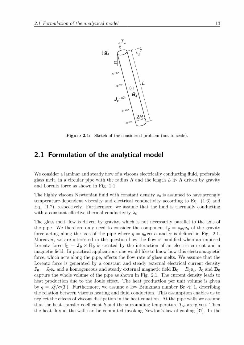
Figure 2.1: Sketch of the considered problem (not to scale).
2.1 Formulation of the analytical model
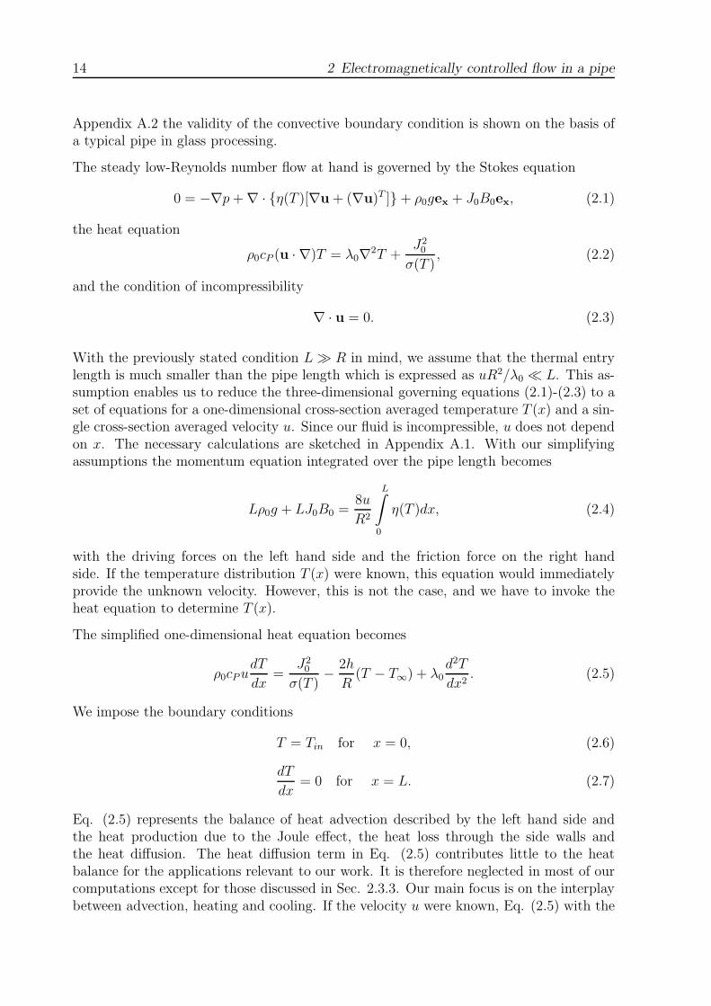
We consider a laminar and steady flow of a viscous electrically conducting fluid, preferableglass melt, in a circular pipe with the radius R and the length L ≫ R driven by gravityand Lorentz force as shown in Fig. 2.1.
The highly viscous Newtonian fluid with constant density ρ0 is assumed to have stronglytemperature-dependent viscosity and electrical conductivity according to Eq. (1.6) andEq. (1.7), respectively. Furthermore, we assume that the fluid is thermally conductingwith a constant effective thermal conductivity λ0.
The glass melt flow is driven by gravity, which is not necessarily parallel to the axis ofthe pipe. We therefore only need to consider the component fg = ρ0gex of the gravityforce acting along the axis of the pipe where g = g0 cos α and α is defined in Fig. 2.1.Moreover, we are interested in the question how the flow is modified when an imposedLorentz force fL = J0 × B0 is created by the interaction of an electric current and amagnetic field. In practical applications one would like to know how this electromagneticforce, which acts along the pipe, affects the flow rate of glass melts. We assume that theLorentz force is generated by a constant and steady external electrical current densityJ0 = J0ey and a homogeneous and steady external magnetic field B0 = B0ez. J0 and B0
capture the whole volume of the pipe as shown in Fig. 2.1. The current density leads toheat production due to the Joule effect. The heat production per unit volume is givenby q = J2
0/σ(T ). Furthermore, we assume a low Brinkman number Br ≪ 1, describingthe relation between viscous heating and fluid conduction. This assumption enables us toneglect the effects of viscous dissipation in the heat equation. At the pipe walls we assumethat the heat transfer coefficient h and the surrounding temperature T∞ are given. Thenthe heat flux at the wall can be computed invoking Newton’s law of cooling [37]. In the
14 2 Electromagnetically controlled flow in a pipe
Appendix A.2 the validity of the convective boundary condition is shown on the basis ofa typical pipe in glass processing.
The steady low-Reynolds number flow at hand is governed by the Stokes equation
0 = −∇p + ∇ · {η(T )[∇u + (∇u)T ]} + ρ0gex + J0B0ex, (2.1)
the heat equation
ρ0cP (u · ∇)T = λ0∇2T +J2
0
σ(T ), (2.2)
and the condition of incompressibility
∇ · u = 0. (2.3)
With the previously stated condition L ≫ R in mind, we assume that the thermal entrylength is much smaller than the pipe length which is expressed as uR2/λ0 ≪ L. This as-sumption enables us to reduce the three-dimensional governing equations (2.1)-(2.3) to aset of equations for a one-dimensional cross-section averaged temperature T (x) and a sin-gle cross-section averaged velocity u. Since our fluid is incompressible, u does not dependon x. The necessary calculations are sketched in Appendix A.1. With our simplifyingassumptions the momentum equation integrated over the pipe length becomes
Lρ0g + LJ0B0 =8u
R2
L∫
0
η(T )dx, (2.4)
with the driving forces on the left hand side and the friction force on the right handside. If the temperature distribution T (x) were known, this equation would immediatelyprovide the unknown velocity. However, this is not the case, and we have to invoke theheat equation to determine T (x).
The simplified one-dimensional heat equation becomes
ρ0cP udT
dx=
J20
σ(T )− 2h
R(T − T∞) + λ0
d2T
dx2. (2.5)
We impose the boundary conditions
T = Tin for x = 0, (2.6)
dT
dx= 0 for x = L. (2.7)
Eq. (2.5) represents the balance of heat advection described by the left hand side andthe heat production due to the Joule effect, the heat loss through the side walls andthe heat diffusion. The heat diffusion term in Eq. (2.5) contributes little to the heatbalance for the applications relevant to our work. It is therefore neglected in most of ourcomputations except for those discussed in Sec. 2.3.3. Our main focus is on the interplaybetween advection, heating and cooling. If the velocity u were known, Eq. (2.5) with the

2.1 Formulation of the analytical model 15
boundary conditions (2.6) and (2.7) would give us T (x). However, u is unknown until wehave solved the remanent of the Stokes equation (2.4). This illustrates the closed-loopinteraction between the velocity and the temperature in our problem.
To cast the governing Eqs. (2.4)-(2.5) into a non-dimensional form the structure of thematerial parameters has to be taken into account. We introduce a non-dimensional tem-perature as follows:
θ =T
E.
Furthermore, we introduce the non-dimensional longitudinal coordinate x′, the non-dimen-sional velocity u′, the control parameters M , P , N , K and the material parameters S, Qaccording to
x′ =x
L, u′ =
8η0
R2ρ0gu, M = 1 +
J0B0
ρ0g, P =
8η0L
ρ20σ0gcPER2
J20 ,
N =16η0L
ρ20gcPR3
h, K =8η0
ρ20gcPR2L
λ0, S =E
A, Q =
B
A.
The forcing parameter M is a measure for the applied Lorentz force in relation to the ef-fective gravity. Changing M is equivalent to changing the applied Lorentz force. Withoutthe Lorentz force M = 1. The parameter P is proportional to the square of the electriccurrent density and therefore a measure of the injected heat. All other quantities enteringP are constant geometry and material parameters. The same is true for N and K. As Nis proportional to h it is a non-dimensional measure for the wall heat loss. The parameterK is a measure for the heat diffusion because of its proportionality to λ0. The parametersS and Q are material parameters related to the electrical conductivity and viscosity.
After performing the nondimensionalisation and dropping the primes we obtain the fol-lowing non-dimensional set of governing equations
M = u
1∫
0
exp
(1
Sθ + Q
)dx, (2.8)
udθ
dx= P exp
(1
θ
)− N(θ − θ∞) + K
d2θ
dx2, (2.9)
θ = θin for x = 0, (2.10)
dθ
dx= 0 for x = 1. (2.11)
The governing equations (2.8)-(2.9) for the considered problem consist of an integral anda second order differential equation which determine the nondimensional velocity u andtemperature distribution θ(x). Eq. (2.8) expresses the balance between the driving forceson the left hand side and the length-integrated viscous friction on the right hand side. Eq.(2.9) represents the balance between advection on the left hand side and Joule heating,wall heat loss, and heat diffusion on the right hand side.
16 2 Electromagnetically controlled flow in a pipe
The governing Eqs. (2.8)-(2.9) are coupled by the temperature θ(x), which appears in thefriction term of the momentum equation because of the considered temperature-dependentviscosity. The second coupling is due to the appearance of u in the heat equation. Equa-tions (2.8) and (2.9) could also be combined into a single integro-differential equation forθ(x) by eliminating u. But we have decided to keep them separate to highlight their originfrom the momentum and heat equation (2.1) and (2.2), respectively. Furthermore, one ofthe parameters M , P , N or K is redundant and can be scaled to 1. We did not applythis scaling to underline the physical source of these parameters.
In the analysis that follows we are most interested in the flow characteristic u as a functionof the forcing parameter M and the temperature field θ(x) under the influence of variousheating parameters P , wall heat loss parameters N , and diffusion parameters K. Therest of Sec. 2 is devoted to the treatment of the system (2.8)-(2.9).
2.2 Solution method
We solve the nonlinear integro-differential set of Eqs. (2.8)-(2.9) using a two-step numer-ical procedure. In the first step the differential equation (2.9) is integrated for an initialguess of the given mean velocity u. If a system without diffusion is investigated, K = 0,the resulting first-order differential equation is solved with a Runge-Kutta method for agiven entrance temperature θin. For this case the second boundary condition, Eq. (2.11),is discarded. The complete second-order differential equation with diffusion is rewrittenas a set of two differential equations of first-order and is solved by applying a shootingmethod to fulfill the boundary conditions. In the course of the shooting procedure thestiff set of equations is solved with an implicit Runge-Kutta method. Shooting from theinlet, x = 0, requires an initial guess for the temperature gradient at x = 0. For u/K ≫ 1the calculated temperature distribution is extremely sensitive to this guess. We observethat the given boundary condition at x = 1 could not be reached even by applying specialroot finding methods like Ridders’ algorithm [62] to determine the initial guess. We haveavoided these convergence problems by shooting from the outlet. We prescribed the out-let temperature θout and varied it using a root finding method to meet the required inlettemperature θin. We found the solution to converge for a wide range of u/K even for arough initial guess of θout and a simple root finding procedure like the bisection method.
In the second step the resulting temperature distribution θ(x) is used to compute theintegral of Eq. (2.8) with the help of the extended trapezoidal rule. For a given forceparameter M , we use a root-finding method to find u so as to obey the governing equations.For a given velocity u, the unknown force M is uniquely determined with Eq. (2.8).
2.3 Selected results 17
100
103
106
10−3
100
103
10−3
M
u
u~M
u~M
u~M1/2
(1) (2) (3)(a)
1000
2000
0 0.2 0.4 0.6 0.8 1
1
1.05
1.1
1.15
x
θ/θ in ≈ ≈
(1)
(2)
(3)
(b)
3000
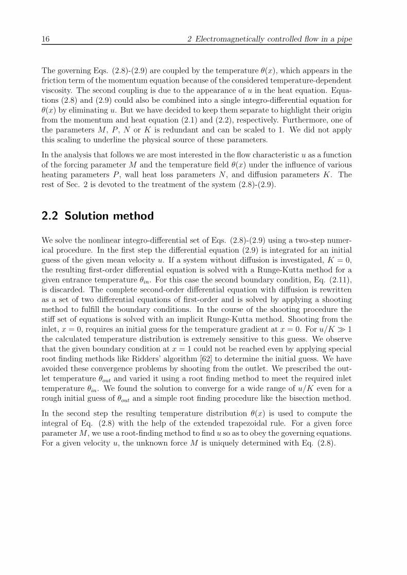
Figure 2.2: Flow regime for internal heating, P = 1, no wall heat loss, N = 0, no diffusion,K = 0 and S = θin = 1, Q = −0.85: (a) Velocity u as a function of the forcing parameterM being the solution of Eqs. (2.8)-(2.9). The curve is divided into three branches: for low(1) and high velocities (3) the relation u ∼ M is fulfilled. For intermediate velocities (2) ascaling u ∼ M1/2 is found as indicated by the dashed lines. (b) Representative distribution ofnormalized temperature θ/θin along x for each of the branches defined in (a).
2.3 Selected results
2.3.1 Heating without wall heat loss
In this part we discuss our results for a system without wall heat loss, N = 0, and withoutheat diffusion, K = 0. The material parameters are set to S = 1 and Q = −0.85 while theinlet temperature is set to θin = 1, respectively. This case is characterized by a balancebetween advection and Joule heating. Fig. 2.2(a) shows the dependence of the velocityon the forcing parameter for one heating parameter. In Fig. 2.2(b) the temperaturedistribution normalized to the inlet temperature for slow, moderate and high velocities isplotted. In general, the velocity u is a monotonically increasing function of the forcingparameter M . For low and high forces the velocity is proportional to the force u ∼ M asit is known from laminar pipe flow with constant material parameters. But in betweenthese linear domains we find that the velocity varies as u ∼ M1/2.
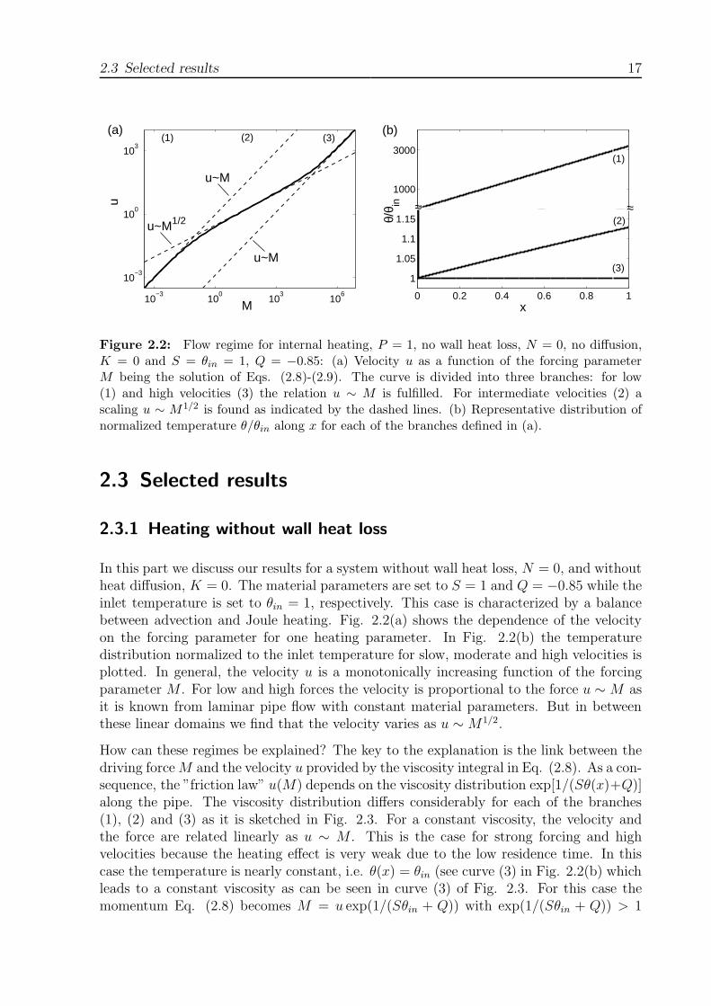
How can these regimes be explained? The key to the explanation is the link between thedriving force M and the velocity u provided by the viscosity integral in Eq. (2.8). As a con-sequence, the ”friction law” u(M) depends on the viscosity distribution exp[1/(Sθ(x)+Q)]along the pipe. The viscosity distribution differs considerably for each of the branches(1), (2) and (3) as it is sketched in Fig. 2.3. For a constant viscosity, the velocity andthe force are related linearly as u ∼ M . This is the case for strong forcing and highvelocities because the heating effect is very weak due to the low residence time. In thiscase the temperature is nearly constant, i.e. θ(x) = θin (see curve (3) in Fig. 2.2(b) whichleads to a constant viscosity as can be seen in curve (3) of Fig. 2.3. For this case themomentum Eq. (2.8) becomes M = u exp(1/(Sθin + Q)) with exp(1/(Sθin + Q)) > 1
18 2 Electromagnetically controlled flow in a pipe
0 0.2 0.4 0.6 0.8 1
0
200
400
600
800
x
exp((
Rq
+Q
)-1)
(1)
(2)
(3)
Figure 2.3: Examples of the distribution of the non-dimensional viscosity exp (1/(Sθ + Q))along the pipe axis x for the branches (1), (2) and (3) defined in Fig. 2.2(a) and obtained withthe same set of parameters.
for (Sθin + Q) > 0 and provides the desired linear relationship on branch (3). For verylow velocities, corresponding to branch (1) in Fig. 2.2(a), the viscosity does not changealong the pipe either. In this case the melt is heated up very quickly as soon as it entersthe pipe. This leads to a very high electrical conductivity and very low Joule heating,respectively. As a result of the high temperatures in this branch, the viscosity jumpsquickly to its lowest possible value corresponding to exp((Sθ + Q)−1) → 1 and remainsvirtually constant along x. This effect is seen in curve (1) of Fig. 2.3. The force M at-tains its theoretically lowest possible value and we have M = u. For moderate velocities,i.e. between the two linear flow regimes (1) and (3), the relationship between M and ubecomes nonlinear as the temperature distribution – and hence the viscosity integral – issensitive to velocity changes.
An explanation of these phenomena can also be given on the basis of an asymptotic alge-braic solution to Eqs. (2.8)-(2.9). This solution has the virtue to display the interactionbetween the temperature-dependent viscosity and the driving forces in its purest form.First we expand the temperature in x around the pipe entrance, e.g. θ ≈ θin + dθ
dxx, to
obtain a linear temperature distribution. With the derivative dθ/dx evaluated from theheat balance given by Eq. (2.9), the linearized temperature field becomes
θ = θin +
{P
uexp
(1
θin
)}x. (2.12)
This expression is valid for moderate and large velocities as its derivation requires u ≫P/θin exp(1/θin). Although Eq. (2.12) is a crude simplification, it shows the influenceof the the parameters on the temperature distribution along the pipe. The temperaturegradient increases with the heating parameter P , but decreases with velocity u due to areduced residence time. The temperature gradient depends strongly on the inlet temper-ature θin due to the exponential temperature-dependence of the electrical conductivity.Particularly for a low inlet temperature θin ≪ 1 the temperature gradient is stronglyamplified since exp(1/θin) ≫ 1. Using Eq. (2.12) the momentum equation (2.8) simplifies

2.3 Selected results 19
to
M = u
1∫
0
exp
1
Sθin + Q· 1
1 + SPSθin+Q
1u
exp(
1θin
)x
dx. (2.13)
With
Z =1
Sθin + Q, M =
M
SPZexp
{−Z − 1
θin
},
u =u
SPZexp
{− 1
θin
}and X =
x
u
Eq. (2.13) becomes
M = u2
1/u∫
0
exp
{− ZX
1 + X
}dX. (2.14)
Thus our problem can be considered as a Laplace-type integral of the form I(Z) =b∫
a
f(X) exp{Zφ(X)}dX with f(X) = 1 and φ(X) = −X/(1 + X). The coefficient Z
characterizes the viscosity at the pipe entrance x = 0 whose non-dimensional value is
ηin = exp
{1
Sθin + Q
}. (2.15)
Now we assume that this viscosity is very large which is equivalent to X → ∞. Withthis assumption we are able to solve the integral I(Z) by integration by parts leading toI(Z) ≈ f(X) exp{Zφ(X)}/(Zφ′(X)) |ba as it is explained in ref. [2]. Observe that thisasymptotic evaluation of the Laplace-type integral does not require the function φ(X) tohave any particular property apart from steadiness. After applying this method for fixedu with O(1/Z) correction and an additional transformation with M = M/Z and u = u/Zwe obtain
M = u2
[1 − exp
(−1
u
)]. (2.16)
Already this simple and compact algebraic equation describes a very interesting flowbehavior, which is shown in Fig. 2.4. For u ≫ 1 one can use the linear expansionexp(−1/u) = 1 − 1/u of the exponential function in which case Eq. (2.16) becomes
u ∼ M . For this case the velocity u is proportional to M as expected for a laminar flow. Incontrast, for u ≪ 1 the exponential function in Eq. (2.16) tends to zero, exp(−1/u) → 0.
As a result the velocity changes according to u ∼ M1/2.
However, this approximation requires moderate and big velocities and very big entrancevalues of the viscosity ηin → ∞. For very small velocities, which is equivalent to X ≫ Z,Eq. (2.16) misses an O(exp(−Z)/u) correction from the solved integral approximation.This explains why it does not reproduce branch (1) and shows a nonlinear behaviorM ∼ u2 for small velocities in contrast to the exact solution. A direct comparisonbetween the analytical and exact solutions for one set of parameters is shown in Fig. 2.5.
20 2 Electromagnetically controlled flow in a pipe
10−10
10−5
100
105
10−5
100
105
~
~M
u
Figure 2.4: Transition between linear and nonlinear friction law for a short pipe: Velocity u
as a function of the force M as obtained from solving Eq. (2.16). The curve is divided into two
branches: for strong forces M ≫ 1 the velocity changes according to u ∼ M as for ordinarylaminar pipe flow with constant material parameters. For weak forces M ≪ 1 the relationu ∼ M1/2 is fulfilled.
100
103
106
10−3
10−3
100
103
M
u
uap
uex
(a)
100
103
106
10−3
0
10
20
30
40
M
∆u/u
ex
(b)
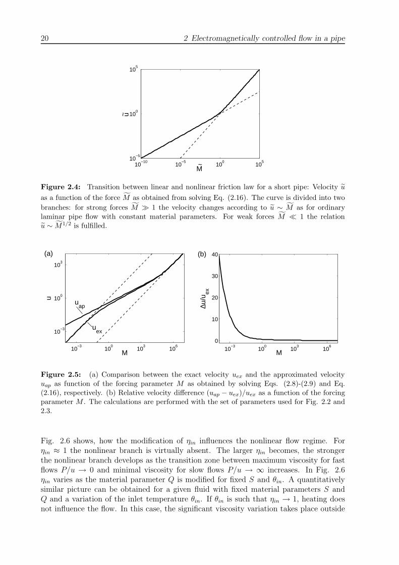
Figure 2.5: (a) Comparison between the exact velocity uex and the approximated velocityuap as function of the forcing parameter M as obtained by solving Eqs. (2.8)-(2.9) and Eq.(2.16), respectively. (b) Relative velocity difference (uap − uex)/uex as a function of the forcingparameter M . The calculations are performed with the set of parameters used for Fig. 2.2 and2.3.
Fig. 2.6 shows, how the modification of ηin influences the nonlinear flow regime. Forηin ≈ 1 the nonlinear branch is virtually absent. The larger ηin becomes, the strongerthe nonlinear branch develops as the transition zone between maximum viscosity for fastflows P/u → 0 and minimal viscosity for slow flows P/u → ∞ increases. In Fig. 2.6ηin varies as the material parameter Q is modified for fixed S and θin. A quantitativelysimilar picture can be obtained for a given fluid with fixed material parameters S andQ and a variation of the inlet temperature θin. If θin is such that ηin → 1, heating doesnot influence the flow. In this case, the significant viscosity variation takes place outside

2.3 Selected results 21
100
103
106
10−3
10−3
100
103
M
u
ηin
Figure 2.6: Velocity of a heated system with P = S = θin = 1 and different materialparameters Q = 0,−0.425,−0.85 leading to ηin = 2.72, 5.69, 785.77. The curves visualize howthe set of parameters Q, S, θin influences the development of the nonlinear flow regime. Forηin → ∞, a flow regime with u ∼ M1/2 develops between the two linear branches.
of the chosen temperature range. Furthermore, Fig. 2.6 visualizes that the wider thegap between the two linear branches of u(M) becomes, the better the nonlinear branchdevelops.
Nonlinear flow we find for ηin > 1 with M ∼ ub, 1 < b ≤ 2 as the viscosity decreasesfor lower velocities. The upper bound of the branch b = 2 is formed because of theproportionality between the slope of the viscosity curve at the pipe entrance s and thevelocity u. This case is reached if (Sθin + Q) → 0 such that ηin ≫ 1. For ηin = 1 theviscosity is constant for all velocities and no nonlinear flow can be observed at all, b = 1.
2.3.2 Heating with wall heat loss
We now turn to the discussion of results for a system with wall heat loss N > 0 andQ = θ∞ = 0. As soon as the assumption N = 0 is abandoned and the viscosity stronglydepends on temperature, we discover a dramatic qualitative change in the behavior of thesystem. Indeed, Fig. 2.7(a) shows that for sufficiently strong heat loss the curve u(M)ceases to be a monotonic function and bifurcations occur. The curve can again be dividedinto 3 branches. For large values of u, branch (3), the wall heat loss and Joule heat donot influence the temperature since the residence time in the pipe is too short. Due tothe constant temperature the velocity u is proportional to M . The same is found forvery small forces, as can be seen by inspecting branch (1) in Fig. 2.7(a). The reason forthe linear behavior on branch (1) is similar to the case N = 0 but it involves a subtledifference resulting from the interplay between wall cooling and Joule heating. In this casethe temperature decreases very fast at the entrance of the pipe. For a lower temperaturethe heat loss is reduced and the electrical heat production is enhanced due to a lowerelectrical conductivity until a temperature is reached, for which the generated heat andthe lost heat are balanced. The constant pipe temperature in this branch does not depend

22 2 Electromagnetically controlled flow in a pipe
104
105
101
102
103
104
M
u
u~M
u~M
(a)(3)
(2)
(1)
0 0.2 0.4 0.6 0.8 10
0.2
0.4
0.6
0.8
1
x
θ/θ in
(b)(3)
(1)
(2)
Figure 2.7: Flow regime for a pipe for the case N = 1000 when the wall heat loss exceeded acritical value NC = 52.2 (remaining parameters: P = S = θin = 1, K = Q = 0): (a) Velocity uas function of the forcing parameter M as obtained by solving Eqs. (2.8)-(2.9). The curve showsthe development of a bifurcation and is divided into 3 branches: the stable branches (1) and (3)with u ∼ M and the unstable branch (2). (b) Representative relative temperature distributionθ(x)/θin along the pipe axis x for every branch.
on the forcing parameter at all, as the left horizontal part of the curves with N 6= 0 inFig. 2.8(b) shows. The constant pipe temperature just depends on the parameters P , Nand θ∞ according to P/N exp(1/θ) = θ−θ∞, see Eq. (2.9) with dθ/dx = 0. Branch (2) ischaracterized by a continuously decreasing shape of θ(x), see Fig. 2.7(b), curve (2). Here,in contrast to branches (1) and (3), the velocity decreases with increasing forces. Thereason is the temperature dependent viscosity. Indeed, a decreasing velocity leads to adecrease of the mean temperature, since the heat loss increases. The result is an increaseof the mean viscosity and finally a significant increase of the driving force required tomaintain the flow.
This mechanism of bifurcation, namely the effect of viscosity and temperature on themean velocity, was already observed in previous studies, e.g. in [86], [30], [87]. But thesestudies consider systems which were cooled only, whereas heating was not included at all.Therefore, the lower stable branch obtained in these studies is not a result of balancedheating and cooling. There, branch (1) is reached as soon as the fluid temperature matchesthe ambient temperature. As a result the ambient temperature is the only parameterdefining the fluid temperature and finally the flow rate for a given forcing parameter dueto the temperature-dependent viscosity. Our studies show that additional heating gives asecond control parameter for the fluid temperature and flow on the lower stable branch.Lange & Loch [48] have not observed the lower stable branch at all.
What would happen if we would experimentally analyze this flow? Let us therefore carryout a thought experiment. We start from branch (3) with a high force and reduce Muntil we reach the left inflexion point in Fig. 2.7(a). Instability will occur due to thefact that a small incidental reduction of u leads to a strong cooling. This, in turn, resultsin a greater viscosity and higher friction force, which reduces the velocity. The greater

2.3 Selected results 23
100
102
104
100
102
104
M
u(a)
N
N=0
100
102
104
0
0.5
1
1.5
M
θ out/θ
in
(b)
N=0
N
Figure 2.8: Influence of the wall heat loss parameter N : (a) Velocity u as function of theforcing parameter M as solution of Eqs. (2.8)-(2.9) for different wall heat loss parametersN = 0, 10, 102 , 103 (remaining parameters: P = S = θin = 1, K = Q = 0). (b) Correspondingrelative exit temperature θout/θin versus acting force M .
residence time intensifies the heat loss which causes an amplification of the slowdownprocess. This self-induced process stops when the heat loss is equal to the increasing heatproduction due to the decreasing electrical conductivity of the fluid. This process appearsas a jump from branch (3) to branch (1) as indicated by the left arrow in Fig. 2.7(a). Wecan also carry out a reverse thought experiment starting with a low force and increasingit until the right inflexion point is reached. At this point, due to the lower residence time,the fluid does not cool down immediately. Heat production and wall heat loss are notbalanced anymore. With the decreasing viscosity the velocity increases which reduces theheat loss and amplifies the acceleration process. This process stops when the temperaturebecomes constant along the pipe and appears as a jump from branch (1) to branch (3).As already studied in [87], branch (2) is unstable in contrast to branches (1) and (3).
In Fig. 2.8 the transition from a system without heat loss to a system with heat loss forvarious heat loss parameters N and constant heat production is shown. A quantitativelyidentical picture could be given for constant heat loss and different heating parametersP . This fact nicely confirms that the temperature on the lower branch is determined bythe balance of heating and cooling, see Fig. 2.8(b), left part of the curves. The higher Nthe lower the temperature and the lower the mean viscosity. A higher force is necessaryto reach a certain velocity, as shown by the lower part of the curves in Fig. 2.8(a).
Fig. 2.9 summarizes the behavior of the system in the two-dimensional space of thecontrol parameters (N/P, M/P ). Within the marked space to the right of the criticalvalue NC/P multiple solutions do coexist. The upper (lower) boundary of this parameterregion marks the value of M for which the solution jumps from one mode to the otherwhen M is increased (decreased). Above the upper boundary one solution of the fast modewith a constant temperature distribution exists. Below the lower boundary one solutionof the slow mode with a constant temperature distribution exists due to balanced heatloss and heat production.
24 2 Electromagnetically controlled flow in a pipe
200 400 600 800
2000
4000
6000
8000
10000
N/P
M/P
Fast Mode
NC
/P
MultipleSolutions
MC
/P
Slow Mode
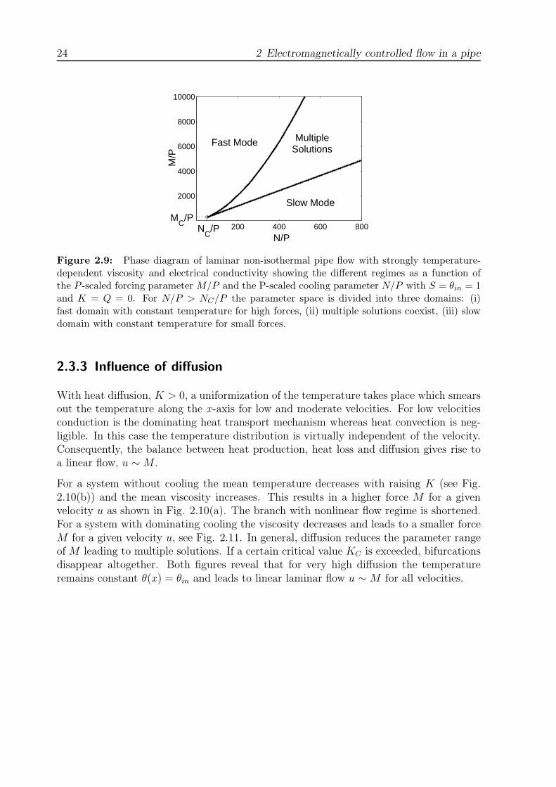
Figure 2.9: Phase diagram of laminar non-isothermal pipe flow with strongly temperature-dependent viscosity and electrical conductivity showing the different regimes as a function ofthe P -scaled forcing parameter M/P and the P-scaled cooling parameter N/P with S = θin = 1and K = Q = 0. For N/P > NC/P the parameter space is divided into three domains: (i)fast domain with constant temperature for high forces, (ii) multiple solutions coexist, (iii) slowdomain with constant temperature for small forces.
2.3.3 Influence of diffusion
With heat diffusion, K > 0, a uniformization of the temperature takes place which smearsout the temperature along the x-axis for low and moderate velocities. For low velocitiesconduction is the dominating heat transport mechanism whereas heat convection is neg-ligible. In this case the temperature distribution is virtually independent of the velocity.Consequently, the balance between heat production, heat loss and diffusion gives rise toa linear flow, u ∼ M .
For a system without cooling the mean temperature decreases with raising K (see Fig.2.10(b)) and the mean viscosity increases. This results in a higher force M for a givenvelocity u as shown in Fig. 2.10(a). The branch with nonlinear flow regime is shortened.For a system with dominating cooling the viscosity decreases and leads to a smaller forceM for a given velocity u, see Fig. 2.11. In general, diffusion reduces the parameter rangeof M leading to multiple solutions. If a certain critical value KC is exceeded, bifurcationsdisappear altogether. Both figures reveal that for very high diffusion the temperatureremains constant θ(x) = θin and leads to linear laminar flow u ∼ M for all velocities.
2.3 Selected results 25
100
103
106
10−3
10−3
100
103
M
u
K
K=0
(a)
100
103
106
10−3
1
2
3
4
5
6
7
M
θ out/θ
in
K K=0
(b)
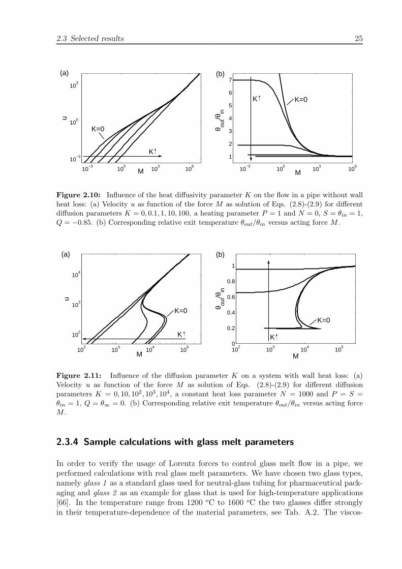
Figure 2.10: Influence of the heat diffusivity parameter K on the flow in a pipe without wallheat loss: (a) Velocity u as function of the force M as solution of Eqs. (2.8)-(2.9) for differentdiffusion parameters K = 0, 0.1, 1, 10, 100, a heating parameter P = 1 and N = 0, S = θin = 1,Q = −0.85. (b) Corresponding relative exit temperature θout/θin versus acting force M .
102
103
104
105
102
103
104
M
u
(a)
K=0
K
102
104
103
105
0
0.2
0.4
0.6
0.8
1
M
θ out/θ
in
(b)
K
K=0
Figure 2.11: Influence of the diffusion parameter K on a system with wall heat loss: (a)Velocity u as function of the force M as solution of Eqs. (2.8)-(2.9) for different diffusionparameters K = 0, 10, 102 , 103, 104, a constant heat loss parameter N = 1000 and P = S =θin = 1, Q = θ∞ = 0. (b) Corresponding relative exit temperature θout/θin versus acting forceM .
2.3.4 Sample calculations with glass melt parameters
In order to verify the usage of Lorentz forces to control glass melt flow in a pipe, weperformed calculations with real glass melt parameters. We have chosen two glass types,namely glass 1 as a standard glass used for neutral-glass tubing for pharmaceutical pack-aging and glass 2 as an example for glass that is used for high-temperature applications[66]. In the temperature range from 1200 oC to 1600 oC the two glasses differ stronglyin their temperature-dependence of the material parameters, see Tab. A.2. The viscos-

26 2 Electromagnetically controlled flow in a pipe
−10 0 10 20−5
0
5
10
15x 10
−3
u [m
/s]
B0 [T]
−10 0 10 20900
1000
1200
1300
Tou
t [°C
]
Tout
u
(a)
−20 −10 0 10 200
5
10
15
20
25
u [m
/s]
B0 [T]
−20 −10 0 10 20
1400
1600
Tou
t [°C
]Tout
u
(b) x 10−3
Figure 2.12: Example calculation for velocity u in m/s and exit temperature Tout in Kas function of the magnetic field density B0 in T for (a) glass 1, and (b) glass 2 with thethermophysical properties listed in Tab. A.2 and the following set of parameters: J0 = 103
A/m2, h = 10 W/m2K, Tin = 13004 oC, T∞ = 20 oC, L = 1 m, R = 0.025 m. For glass 1 heatloss dominates and bifurcation occurs. Due to the low electrical conductivity of glass 2 heatproduction dominates and the solution is unique.
ity of glass 1 varies between 700 Pas and 25 Pas and the electrical conductivity variesbetween 4.2 S/m and 12.6 S/m. Glass 2 is characterized by a viscosity decrease from2110 Pas to 6.5 Pas and a very low electrical conductivity, increasing from 2.6 · 10−2 S/mto 1.2 S/m. The calculations have been performed for the following common parameters:J0 = 103 A/m2, h = 10 W/m2K, Tin = 1300 oC, T∞ = 20 oC for a pipe with a length ofL = 1 m, and a radius of R = 0.025 m.
With this set of parameters, the wall heat loss dominates for glass 1 and leads to bifur-cation as shown in Fig. 2.12(a). If we assume an operating range of −3T ≤ B0 ≤ 3T thevelocity of the upper stable branch can be controlled between 4.4·10−3m/s ≤ u ≤ 6.5·10−3
m/s. It enables a continuous fine tuning of the mass flow rate. At the lower branch thefluid has a low constant temperature and is almost immobilized. In accordance with thetheoretical results of the previous section, the velocity of these two branches varies linearlywith the external magnetic field. Due to the low electrical conductivity of glass 2 theheat production dominates and no bifurcation occurs as shown in Fig. 2.12(b). The heatproduction is so large that the temperature increases by more than 100 K. In order tocool the melt the applied current density can be reduced. It would lead to a small, almostnegligible Lorentz force density in the melt. Alternatively the cooling of the system canbe increased with an additional cooling system to balance the heat production. In bothcases, however, bifurcation occurs if the cooling rate is strong enough.
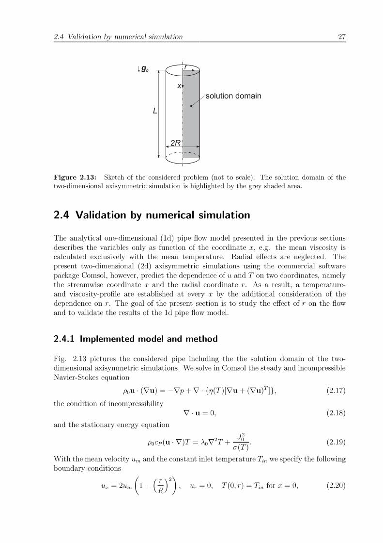
2.4 Validation by numerical simulation 27
x
r
L
2R
solution domain
g0
Figure 2.13: Sketch of the considered problem (not to scale). The solution domain of thetwo-dimensional axisymmetric simulation is highlighted by the grey shaded area.
2.4 Validation by numerical simulation
The analytical one-dimensional (1d) pipe flow model presented in the previous sectionsdescribes the variables only as function of the coordinate x, e.g. the mean viscosity iscalculated exclusively with the mean temperature. Radial effects are neglected. Thepresent two-dimensional (2d) axisymmetric simulations using the commercial softwarepackage Comsol, however, predict the dependence of u and T on two coordinates, namelythe streamwise coordinate x and the radial coordinate r. As a result, a temperature-and viscosity-profile are established at every x by the additional consideration of thedependence on r. The goal of the present section is to study the effect of r on the flowand to validate the results of the 1d pipe flow model.
2.4.1 Implemented model and method
Fig. 2.13 pictures the considered pipe including the the solution domain of the two-dimensional axisymmetric simulations. We solve in Comsol the steady and incompressibleNavier-Stokes equation
ρ0u · (∇u) = −∇p + ∇ · {η(T )[∇u + (∇u)T ]}, (2.17)
the condition of incompressibility∇ · u = 0, (2.18)
and the stationary energy equation
ρ0cP (u · ∇)T = λ0∇2T +J2
0
σ(T ). (2.19)
With the mean velocity um and the constant inlet temperature Tin we specify the followingboundary conditions
ux = 2um
(1 −
( r
R
)2)
, ur = 0, T (0, r) = Tin for x = 0, (2.20)
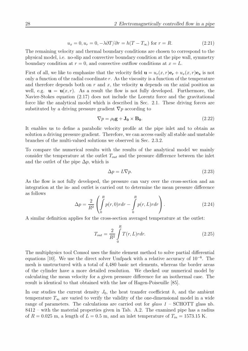
28 2 Electromagnetically controlled flow in a pipe
ux = 0, ur = 0,−λ∂T/∂r = h(T − T∞) for r = R. (2.21)
The remaining velocity and thermal boundary conditions are chosen to correspond to thephysical model, i.e. no-slip and convective boundary condition at the pipe wall, symmetryboundary condition at r = 0, and convective outflow conditions at x = L.
First of all, we like to emphasize that the velocity field u = ur(x, r)er + ux(x, r)ex is notonly a function of the radial coordinate r. As the viscosity is a function of the temperatureand therefore depends both on r and x, the velocity u depends on the axial position aswell, e.g. u = u(x, r). As a result the flow is not fully developed. Furthermore, theNavier-Stokes equation (2.17) does not include the Lorentz force and the gravitationalforce like the analytical model which is described in Sec. 2.1. These driving forces aresubstituted by a driving pressure gradient ∇p according to
∇p = ρ0g + J0 × B0. (2.22)
It enables us to define a parabolic velocity profile at the pipe inlet and to obtain assolution a driving pressure gradient. Therefore, we can access easily all stable and unstablebranches of the multi-valued solutions we observed in Sec. 2.3.2.
To compare the numerical results with the results of the analytical model we mainlyconsider the temperature at the outlet Tout and the pressure difference between the inletand the outlet of the pipe ∆p, which is
∆p = L∇p. (2.23)
As the flow is not fully developed, the pressure can vary over the cross-section and anintegration at the in- and outlet is carried out to determine the mean pressure differenceas follows
∆p =2
R2
R∫
0
p(r, 0)rdr −R∫
0
p(r, L)rdr
. (2.24)
A similar definition applies for the cross-section averaged temperature at the outlet:
Tout =2
R2
R∫
0
T (r, L)rdr. (2.25)
The multiphysics tool Comsol uses the finite element method to solve partial differentialequations [10]. We use the direct solver Umfpack with a relative accuracy of 10−6. Themesh is unstructured with a total of 4,480 basic net elements, whereas the border areasof the cylinder have a more detailed resolution. We checked our numerical model bycalculating the mean velocity for a given pressure difference for an isothermal case. Theresult is identical to that obtained with the law of Hagen-Poiseuille [85].
In our studies the current density J0, the heat transfer coefficient h, and the ambienttemperature T∞ are varied to verify the validity of the one-dimensional model in a widerange of parameters. The calculations are carried out for glass 1 – SCHOTT glass nb.8412 – with the material properties given in Tab. A.2. The examined pipe has a radiusof R = 0.025 m, a length of L = 0.5 m, and an inlet temperature of Tin = 1573.15 K.
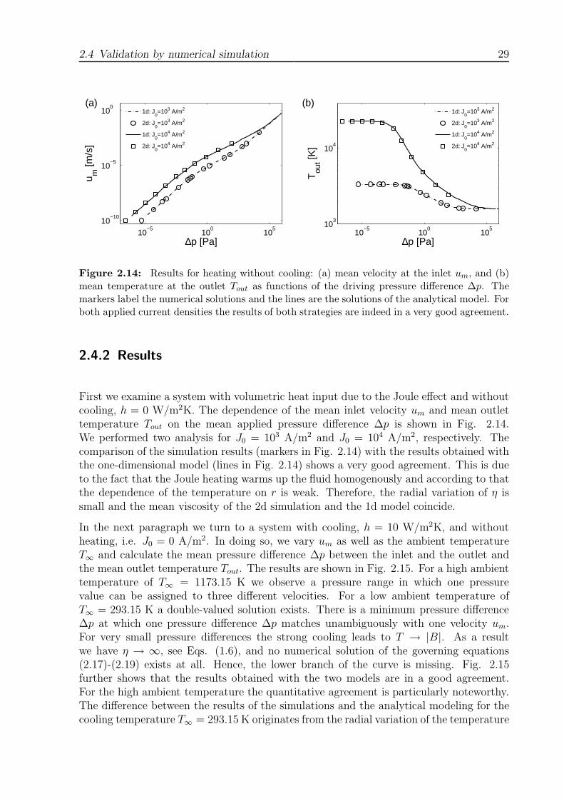
2.4 Validation by numerical simulation 29
10−5
100
105
10−10
10−5
100
∆p [Pa]
u m [m
/s]
1d: J0=103 A/m2
2d: J0=103 A/m2
1d: J0=104 A/m2
2d: J0=104 A/m2
(a)
10−5
100
105
103
104
∆p [Pa]
Tou
t [K]
1d: J0=103 A/m2
2d: J0=103 A/m2
1d: J0=104 A/m2
2d: J0=104 A/m2
(b)
Figure 2.14: Results for heating without cooling: (a) mean velocity at the inlet um, and (b)mean temperature at the outlet Tout as functions of the driving pressure difference ∆p. Themarkers label the numerical solutions and the lines are the solutions of the analytical model. Forboth applied current densities the results of both strategies are indeed in a very good agreement.
2.4.2 Results
First we examine a system with volumetric heat input due to the Joule effect and withoutcooling, h = 0 W/m2K. The dependence of the mean inlet velocity um and mean outlettemperature Tout on the mean applied pressure difference ∆p is shown in Fig. 2.14.We performed two analysis for J0 = 103 A/m2 and J0 = 104 A/m2, respectively. Thecomparison of the simulation results (markers in Fig. 2.14) with the results obtained withthe one-dimensional model (lines in Fig. 2.14) shows a very good agreement. This is dueto the fact that the Joule heating warms up the fluid homogenously and according to thatthe dependence of the temperature on r is weak. Therefore, the radial variation of η issmall and the mean viscosity of the 2d simulation and the 1d model coincide.
In the next paragraph we turn to a system with cooling, h = 10 W/m2K, and withoutheating, i.e. J0 = 0 A/m2. In doing so, we vary um as well as the ambient temperatureT∞ and calculate the mean pressure difference ∆p between the inlet and the outlet andthe mean outlet temperature Tout. The results are shown in Fig. 2.15. For a high ambienttemperature of T∞ = 1173.15 K we observe a pressure range in which one pressurevalue can be assigned to three different velocities. For a low ambient temperature ofT∞ = 293.15 K a double-valued solution exists. There is a minimum pressure difference∆p at which one pressure difference ∆p matches unambiguously with one velocity um.For very small pressure differences the strong cooling leads to T → |B|. As a resultwe have η → ∞, see Eqs. (1.6), and no numerical solution of the governing equations(2.17)-(2.19) exists at all. Hence, the lower branch of the curve is missing. Fig. 2.15further shows that the results obtained with the two models are in a good agreement.For the high ambient temperature the quantitative agreement is particularly noteworthy.The difference between the results of the simulations and the analytical modeling for thecooling temperature T∞ = 293.15 K originates from the radial variation of the temperature
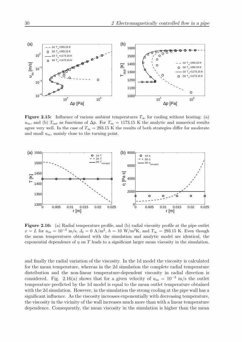
30 2 Electromagnetically controlled flow in a pipe
104
106
10−6
10−4
10−2
100
∆p [Pa]
u m [m
/s]
1d: T∞=293.15 K
2d: T∞=293.15 K
1d: T∞=1173.15 K
2d: T∞=1173.15 K
(a)
104
106
1000
1100
1200
1300
1400
1500
1600
∆p [Pa]
Tou
t [K]
1d: T∞=293.15 K
2d: T∞=293.15 K
1d: T∞=1173.15 K
2d: T∞=1173.15 K
(b)
Figure 2.15: Influence of various ambient temperatures T∞ for cooling without heating: (a)um, and (b) Tout as functions of ∆p. For T∞ = 1173.15 K the analytic and numerical resultsagree very well. In the case of T∞ = 293.15 K the results of both strategies differ for moderateand small um, mainly close to the turning point.
0 0.005 0.01 0.015 0.02 0.0251300
1350
1400
1450
1500
1550
r [m]
T [K
]
1d: T2d: T2d: T
averaged
(a)
0 0.005 0.01 0.015 0.02 0.0250
2000
4000
6000
8000
r [m]
η [P
a s]
1d: η2d: η2d: η
averaged
(b)
Figure 2.16: (a) Radial temperature profile, and (b) radial viscosity profile at the pipe outletx = L for um = 10−3 m/s, J0 = 0 A/m2, h = 10 W/m2K, and T∞ = 293.15 K. Even thoughthe mean temperatures obtained with the simulation and analytic model are identical, theexponential dependence of η on T leads to a significant larger mean viscosity in the simulation.
and finally the radial variation of the viscosity. In the 1d model the viscosity is calculatedfor the mean temperature, whereas in the 2d simulation the complete radial temperaturedistribution and the non-linear temperature-dependent viscosity in radial direction isconsidered. Fig. 2.16(a) shows that for a given velocity of um = 10−3 m/s the outlettemperature predicted by the 1d model is equal to the mean outlet temperature obtainedwith the 2d simulation. However, in the simulation the strong cooling at the pipe wall has asignificant influence. As the viscosity increases exponentially with decreasing temperature,the viscosity in the vicinity of the wall increases much more than with a linear temperaturedependence. Consequently, the mean viscosity in the simulation is higher than the mean
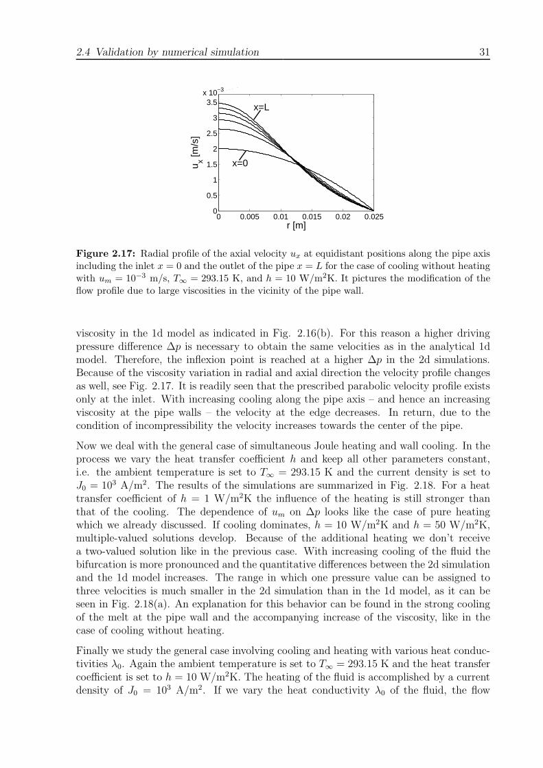
2.4 Validation by numerical simulation 31
0 0.005 0.01 0.015 0.02 0.0250
0.5
1
1.5
2
2.5
3
3.5
x 10−3
r [m]
u x [m/s
]
x 10−3
x=L
x=0
Figure 2.17: Radial profile of the axial velocity ux at equidistant positions along the pipe axisincluding the inlet x = 0 and the outlet of the pipe x = L for the case of cooling without heatingwith um = 10−3 m/s, T∞ = 293.15 K, and h = 10 W/m2K. It pictures the modification of theflow profile due to large viscosities in the vicinity of the pipe wall.
viscosity in the 1d model as indicated in Fig. 2.16(b). For this reason a higher drivingpressure difference ∆p is necessary to obtain the same velocities as in the analytical 1dmodel. Therefore, the inflexion point is reached at a higher ∆p in the 2d simulations.Because of the viscosity variation in radial and axial direction the velocity profile changesas well, see Fig. 2.17. It is readily seen that the prescribed parabolic velocity profile existsonly at the inlet. With increasing cooling along the pipe axis – and hence an increasingviscosity at the pipe walls – the velocity at the edge decreases. In return, due to thecondition of incompressibility the velocity increases towards the center of the pipe.
Now we deal with the general case of simultaneous Joule heating and wall cooling. In theprocess we vary the heat transfer coefficient h and keep all other parameters constant,i.e. the ambient temperature is set to T∞ = 293.15 K and the current density is set toJ0 = 103 A/m2. The results of the simulations are summarized in Fig. 2.18. For a heattransfer coefficient of h = 1 W/m2K the influence of the heating is still stronger thanthat of the cooling. The dependence of um on ∆p looks like the case of pure heatingwhich we already discussed. If cooling dominates, h = 10 W/m2K and h = 50 W/m2K,multiple-valued solutions develop. Because of the additional heating we don’t receivea two-valued solution like in the previous case. With increasing cooling of the fluid thebifurcation is more pronounced and the quantitative differences between the 2d simulationand the 1d model increases. The range in which one pressure value can be assigned tothree velocities is much smaller in the 2d simulation than in the 1d model, as it can beseen in Fig. 2.18(a). An explanation for this behavior can be found in the strong coolingof the melt at the pipe wall and the accompanying increase of the viscosity, like in thecase of cooling without heating.
Finally we study the general case involving cooling and heating with various heat conduc-tivities λ0. Again the ambient temperature is set to T∞ = 293.15 K and the heat transfercoefficient is set to h = 10 W/m2K. The heating of the fluid is accomplished by a currentdensity of J0 = 103 A/m2. If we vary the heat conductivity λ0 of the fluid, the flow

32 2 Electromagnetically controlled flow in a pipe
100
105
10−6
10−4
10−2
100
∆p [Pa]
u m [m
/s]
1d: h=1 W/m2K
2d: h=1 W/m2K
1d: h=10 W/m2K
2d: h=10 W/m2K
1d: h=50 W/m2K
2d: h=50 W/m2K
(a)
100
105
1000
1100
1200
1300
1400
1500
1600
1700
∆p [Pa]
Tou
t [K]
1d: h=1 W/m2K
2d: h=1 W/m2K
1d: h=10 W/m2K
2d: h=10 W/m2K
1d: h=50 W/m2K
2d: h=50 W/m2K
(b)
Figure 2.18: Influence of various heat transfer coefficients h for cooling and heating at thesame time: (a) um and (b) Tout as function of ∆p. The larger h – and hence the cooling rate –the more the solutions of both approaches diverge.
characteristics can change considerably as one can see in Fig. 2.19. In the 1d analyticalmodel bifurcation develops if the conductivity is smaller than a certain critical value, i.e.λ0 < λmax. The smaller λ0, the more distinct the bifurcation is. For λ0 = 0 W/mK thepressure range for which one pressure value can be assigned to three velocities reaches itsmaximum. In contrast in the simulation we obtain a range λmin ≤ λ0 ≤ λmax for whichthe function um(∆p) is not single-valued. For λ0 < λmin and λ0 > λmax every ∆p can beassigned unambiguously to one um. For small values of λ0 differences between the twoapproaches are obvious. The differences result from the assumption that the effects ofthe heat conductivity are only considered along the pipe axis x in the 1d model. Alongthe radial direction r the temperature is assumed to be constant and the ’radial’ heatconductivity is infinity – independent of ’axial’ heat conductivity λ0. In contrast in the2d simulation the heat conduction is acting in x- and r-direction. With increasing λ0 thetemperature profile flattens as shown in Fig. 2.20. If λ0 has reached a certain value, thetemperature in radial direction is almost constant and hence, fulfills the assumptions ofthe 1d model. In this regime the results of both models are in a very good agreement.

2.5 Simple experimental study of a non-magnetic case 33
103
104
105
106
10−6
10−4
10−2
100
∆p [Pa]
u m [m
/s]
1d: λ0=0.25W/mK
2d: λ0=0.25W/mK
1d: λ0=1.2W/mK
2d: λ0=1.2W/mK
1d: λ0=5W/mK
2d: λ0=5W/mK
(a)
103
104
105
106
1200
1300
1400
1500
1600
∆p [Pa]
Tou
t [K]
1d: λ0=0.25W/mK
2d: λ0=0.25W/mK
1d: λ0=1.2W/mK
2d: λ0=1.2W/mK
1d: λ0=5W/mK
2d: λ0=5W/mK
(b)
103
104
105
106
10−6
10−4
10−2
100
∆p [Pa]
u m [m
/s]
1d: λ0=5W/mK
2d: λ0=5W/mK
1d: λ0=30W/mK
2d: λ0=30W/mK
1d: λ0=50W/mK
2d: λ0=50W/mK
(c)
103
104
105
106
1200
1300
1400
1500
1600
∆p [Pa]
Tou
t [K]
1d: λ0=5W/mK
2d: λ0=5W/mK
1d: λ0=30W/mK
2d: λ0=30W/mK
1d: λ0=50W/mK
2d: λ0=50W/mK
(d)
Figure 2.19: Influence of heat conductivity λ0 for cooling and heating at the same time:(a), (c) um and (b), (d) Tout as function of ∆p. For λ0 & 5 W/mK, (c)-(d), the results ofboth strategies are in excellent agreement. But for λ0 . 5 W/mK, (a)-(b), the region of thethree-valued solution increases and therefore agreement is left.
2.5 Simple experimental study of a non-magnetic case
In the following section we like to introduce a simple non-magnetic laboratory experimentof the non-isothermal pipe flow. We don’t focus on an exact verification of the theoryand a direct comparison. Our goal is to detect and measure the upper and lower branchof the multiple-valued solutions which we studied in Sec. 2.3.2.
2.5.1 Experimental setup and procedure
We use glycerin as working fluid which is common for so-called ”cold experiments” of glassmelt flows [70]. The advantage is that the dependence of the viscosity on temperature iscomparable to that of glass melt at room temperature. Like in the numerical simulationswe can approximate the driving Lorentz force and gravitational force by a pressure gra-

34 2 Electromagnetically controlled flow in a pipe
0 0.005 0.01 0.015 0.02 0.0251000
1100
1200
1300
1400
r [m]
T [K
]
2d: λ0=0.25 W/mK
2d: λ0=1.2 W/mK
2d: λ0=50 W/mK
Figure 2.20: Radial temperature profile for various heat conductivities λ0 and um = 10−6
m/s, J0 = 103 A/m2, h = 10 W/m2K, T∞ = 293.15 K. For large λ0 the temperature is constantover the cross section and corresponds to the assumptions of the analytical 1d model.
1
2 3 4
5 5
Figure 2.21: Experimental setup with 1 thermostat, 2 height adjustment, 3 flexible tubewithout heating jacked, 4 double pipe heat exchanger, and 5 head loss measurement.
dient along a horizontal pipe according to Eq. (2.22). Furthermore, the detection of themultiple-valued solutions just requires cooling and no direct electric heating (Heating isnot restricted to direct electrical heating as it is used in the analytical model. In a simpleexperiment the heat can also be inserted over the wall. This procedure would not allowsimultaneous heating and cooling). The configuration of the experiment is shown in Fig.2.21. The heart of the experiment is the double-pipe heat exchanger made of copper.
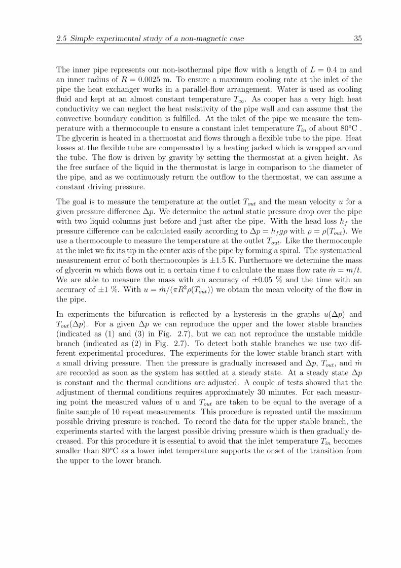
2.5 Simple experimental study of a non-magnetic case 35
The inner pipe represents our non-isothermal pipe flow with a length of L = 0.4 m andan inner radius of R = 0.0025 m. To ensure a maximum cooling rate at the inlet of thepipe the heat exchanger works in a parallel-flow arrangement. Water is used as coolingfluid and kept at an almost constant temperature T∞. As cooper has a very high heatconductivity we can neglect the heat resistivity of the pipe wall and can assume that theconvective boundary condition is fulfilled. At the inlet of the pipe we measure the tem-perature with a thermocouple to ensure a constant inlet temperature Tin of about 80oC .The glycerin is heated in a thermostat and flows through a flexible tube to the pipe. Heatlosses at the flexible tube are compensated by a heating jacked which is wrapped aroundthe tube. The flow is driven by gravity by setting the thermostat at a given height. Asthe free surface of the liquid in the thermostat is large in comparison to the diameter ofthe pipe, and as we continuously return the outflow to the thermostat, we can assume aconstant driving pressure.
The goal is to measure the temperature at the outlet Tout and the mean velocity u for agiven pressure difference ∆p. We determine the actual static pressure drop over the pipewith two liquid columns just before and just after the pipe. With the head loss hf thepressure difference can be calculated easily according to ∆p = hfgρ with ρ = ρ(Tout). Weuse a thermocouple to measure the temperature at the outlet Tout. Like the thermocoupleat the inlet we fix its tip in the center axis of the pipe by forming a spiral. The systematicalmeasurement error of both thermocouples is ±1.5 K. Furthermore we determine the massof glycerin m which flows out in a certain time t to calculate the mass flow rate m = m/t.We are able to measure the mass with an accuracy of ±0.05 % and the time with anaccuracy of ±1 %. With u = m/(πR2ρ(Tout)) we obtain the mean velocity of the flow inthe pipe.
In experiments the bifurcation is reflected by a hysteresis in the graphs u(∆p) andTout(∆p). For a given ∆p we can reproduce the upper and the lower stable branches(indicated as (1) and (3) in Fig. 2.7), but we can not reproduce the unstable middlebranch (indicated as (2) in Fig. 2.7). To detect both stable branches we use two dif-ferent experimental procedures. The experiments for the lower stable branch start witha small driving pressure. Then the pressure is gradually increased and ∆p, Tout, and mare recorded as soon as the system has settled at a steady state. At a steady state ∆pis constant and the thermal conditions are adjusted. A couple of tests showed that theadjustment of thermal conditions requires approximately 30 minutes. For each measur-ing point the measured values of u and Tout are taken to be equal to the average of afinite sample of 10 repeat measurements. This procedure is repeated until the maximumpossible driving pressure is reached. To record the data for the upper stable branch, theexperiments started with the largest possible driving pressure which is then gradually de-creased. For this procedure it is essential to avoid that the inlet temperature Tin becomessmaller than 80oC as a lower inlet temperature supports the onset of the transition fromthe upper to the lower branch.

36 2 Electromagnetically controlled flow in a pipe
0 1000 2000 3000 4000 50000
0.01
0.02
0.03
0.04
0.05
0.06
∆p [Pa]
u [m
/s]
increasingdecreasing
(a)
0 1000 2000 3000 4000 50000
20
40
60
80
∆p [Pa]
Tou
t [o C]
Tin
T∞
increasingdecreasing
(b)
Figure 2.22: Measured data for a cooling temperature of T∞ = 20oC: (a) mean velocity u,and (b) outlet temperature Tout as functions of the pressure loss over the pipe ∆p for − ▽ −increasing and −o− decreasing driving pressure. For the chosen cooling temperature we don’tdetect the desired regime of bifurcation.
1000 2000 3000 4000 5000 60000
0.01
0.02
0.03
0.04
0.05
∆p [Pa]
u [m
/s]
increasingdecreasing
(a)
1000 2000 3000 4000 5000 60000
20
40
60
80
∆p [Pa]
Tou
t [o C]
Tin
T∞
increasingdecreasing
(b)
Figure 2.23: Measured date for a cooling temperature of T∞ = 10oC: (a) u(∆p), and (b)Tout(∆p). In a small band of about 300 Pa we are able to obtain two measuring values for one∆p. It shows that bifurcation exists for T∞ = 10oC and the prescribed conditions.
2.5.2 Results
The experiments are conducted for two cooling temperatures, namely T∞ = 20oC andT∞ = 10oC. The results are pictured in Figs. 2.22 and 2.23. For T∞ = 20oC it isparticularly obvious that we do not measure two different mean velocities and two differentoutlet temperatures for one given ∆p. The curves for an increasing and a decreasingdriving pressure are almost identical. However, for T∞ = 10oC we get two measuringvalues for one ∆p in a small band of about 300 Pa. As predicted by the theory, Tout ofthe lower branch is almost identical to the cooling temperature. Just after passing thelower inflexion point by slightly increasing ∆p from 4060 Pa to 4200 Pa, Tout changes from
2.6 Summary and discussion 37
12oC up to 56oC. The transition from the upper to the lower branch is characterized bya significant jump of the outlet temperature as well. While decreasing ∆p from 3860 Pato 3710 Pa, Tout changes from 43oC to 12oC.
To our knowledge, the bifurcation based on temperature-dependent viscosity has beendetected only by only Whitehead & Helfrich [86]. Whitehead & Helfrich got inspired bylava flow and used corn sirup as working fluid. Even though they observed the hysteresis,the experimental setup and procedure was quiet different. The syrup was driven by thefilling height of a reservoir and flowed from the reservoir through a tube immersed ina chilled bath. The filling height of the reservoir oscillated with time. The oscillationsproduced a close curve in the height-velocity space indication the bifurcation as two-velocities could be obtained for one filling height.
2.6 Summary and discussion
We have formulated an one-dimensional analytical model which describes the interplaybetween friction force, gravity, Lorentz force, heat generation, heat loss, heat transportand heat diffusion in a circular pipe. The model takes into account the exponentialtemperature-dependence of the viscosity and the electrical conductivity. It is a simplifiedrepresentation of electromagnetically controlled glass melt flow in a feeder. Our analysisreveals that the flow characteristics are strongly affected by the variation of the materialparameters along the pipe. For a heated system without heat loss a variation within thetemperature field leads to a velocity u which is not in general a linear function of theacting force M . If the viscosity at the pipe entrance has not reached the lowest possiblevalue ηin > 1, we found a non-linear flow regime such as ub ∼ M with 1 < b ≤ 2. Fora system with additional dominating heat loss three velocities for one given driving forcecan be observed. The velocity ceases to be a single valued function of the acting force andbifurcations exist for a wide range of parameters. Three regimes allow the fluid to haveconstant material parameters and therefore lead to a known laminar flow characteristicwith linear proportionality between the velocity and acting force u ∼ M : (i) the velocityis high, the residence time within the pipe and therefore the temperature change is low;(ii) the temperature is very high so that the viscosity reaches its lowest possible value;(iii) the heat loss and heat generation are balanced.
We have validated the one-dimensional model with two-dimensional axisymmetric simu-lations using the commercial software Comsol. For heating without cooling we found avery good agreement between the results of both approaches. The monotonic, non-linearflow behavior has been predicted correctly by the one-dimensional model. The bifurca-tion, which develops for dominating cooling, has been reproduced by both methods. Butfor this case we found quantitative differences which are a result of larger temperaturegradients and the non-linear increase of the viscosity with decreasing temperature. Fur-thermore, the two-dimensional simulations showed an excellent quantitative agreementwith the prediction of the analytical model for moderate and high heat conductivities λ0.For this case the temperature is almost constant along the cross section in the simulationsand therefore fulfils an important assumption of the analytical model. However, for low

38 2 Electromagnetically controlled flow in a pipe
heat conductivities differences develop. In the one-dimensional model bifurcation existsfor all λ0 ≤ λmax. But in the simulations bifurcation also disappears for very small λ0.Here, bifurcation exists only in a limited range with λmin ≤ λ0 ≤ λmax. Additionally, weconducted a simple non-magnetic laboratory experiment to measure the stable branchesof the bifurcation.
During our studies of the presented model we focused on the description and explanationof the new laminar flow characteristics. We did not particularly emphasize the importanceof the results for the flow control. Now we will catch up on this briefly. To increase thevelocity of a heated system by factor a, the driving force has to be increased by factorab with 1 ≤ b ≤ 2. In this regime the change of forces is higher than for linear laminarflow. The observed bifurcation for a system with dominant cooling provide a new wayof flow control. In the vicinity of the two inflexion points a weak change of the actingforce leads to a significant change of the velocity. The coexistent temperature jumpwhich is the reason for the bifurcation may lead to significant and unintended materialchanges. However, we observed that one stable branch is reached for a balance of coolingand heating. Hence, the heating can be used to control the position of the lower stablebranch. This mechanism enables the active external regulation of the development of thebifurcation and therefore the characteristics of the temperature and velocity jumps in thevicinity of the inflexion points. Furthermore, we identified various regimes in which thevelocity is a linear function of the driving force - hence the imposed Lorentz force. Thislinear functionality allows for a precise and simple electromagnetic control of the glassmelt flow.

3 Electromagnetically controlled flow in
a crucible
Now we leave the subject of electromagnetically controlled forced convection in a pipeand concentrate on free convection in a small scale crucible which is influenced by theimposed Lorentz force. The electromagnetically controlled free convection is relevantfor glass processing as it provides new possibilities to increase mixing and to improvethe temperature homogenization. We consider a setup which was used for experimentalstudies by Krieger and co-workers [35], [42]. They have visualized the flow pattern andhave proven the influence of the imposed Lorentz force e.g. by temperature measurementsat a limited number of positions within the melt. However, the experiments are not ableto answer the following questions: How is the transition from a purely buoyant drivenflow to a mainly Lorentz force driven flow characterized and how are the flow patternand temperature distribution influenced by the Lorentz force? Moreover, one would liketo know the scale relations between the velocity, temperature, and Lorentz force andwhether the temperature-dependent material properties of glass melts influence the flowcharacteristic. In the following we will give answers to these questions by means ofthree-dimensional (3d) numerical parameter studies in Sec. 3.1 and one-dimensional (1d)analytical modeling in Sec. 3.2. In Sec. 3.3 we perform some sample calculations tocompare the numerical, analytical, and experimental results.
3.1 Three-dimensional numerical simulation
The present approach is to study systematically the electromagnetically controlled ther-mal convection of glass melt in a small scale cylindrical crucible. The current density isgenerated by two rod electrodes, which are immersed into the melt. Therefore, papers onmathematical modeling of electric furnaces are relevant for our numerical studies, whichnumber is limited. In the following we will briefly introduce these papers. In his pioneer-ing work Curran [12] studied the effects of different electrode configurations in a 2d modelfollowed by Austin & Bourne [1], and Mardorf [50] who included a feeding rate of thebatch. Chen & Goodson [6] presented 3d results assuming constant material propertiesexcept in the buoyancy term. Between 1986 and 1988 some papers about 3d simulationsof industrial all-electric furnaces were published [7], [78] [79], [80], [8]. The authors ofthese papers focused on the arrangement and orientation of multiple electrodes. Further-more, they included the pull rate of the batch and the temperature-dependent materialproperties. Due to the limited computational power at that time the grid refinement wasextremely limited. With combined experimental and three-dimensional numerics Hiejima
39

40 3 Electromagnetically controlled flow in a crucible
Figure 3.1: Sketch of the considered problem (not to scale).
[31] studied the possibilities to control the glass convection with various electric boostingconditions, heat loss through the walls, and the charged glass batch. Recently, the setupof a small scale cylindrical crucible was modeled numerically by Cepite and co-workersin [5]. The authors used idealized and unrealistic thermal boundary conditions to meetthe experimental data of [35], [42]. Even more, they did not perform any systematicvariations of the Lorentz force magnitude and can not give any answer to the questionswe just posed.
3.1.1 Formulation of the problem
The small scale crucible which we consider is sketched in Fig. 3.1. The inner radius ofthe laboratory crucible is R = 0.04 m and the fill level of the molten glass is H = 0.08 m.Two rod electrodes with a diameter of D = 0.013 m are symmetrically immersed 0.06 minto the melt from the top at (x, y) = (−0.0165 m, 0 m) and at (x, y) = (0.0165 m, 0 m).The prescribed setup has two symmetry planes, namely the plane x = 0 m and the planey = 0 m which are shown in Fig. 3.2.
The glass melt is assumed to be Newtonian with a constant heat capacity cP and theviscosity η(T ) and the electrical conductivity σ(T ) being exponential functions of thetemperature T according to Eqs. (1.6) and (1.7), respectively. Furthermore, the density(T ) is assumed to be a linear function of the temperature and the heat conductivity λ(T )is approximated by a quadratic function of the temperature.
Between the electrodes a constant electric potential difference UE is applied. As a resultwe obtain a current density distribution J which is heating the melt due to the Jouleeffect with the volumetric heat input J2/σ. As we have heat losses at the surface andthe crucible walls, temperature and density gradients develop in the melt. Thus, with the
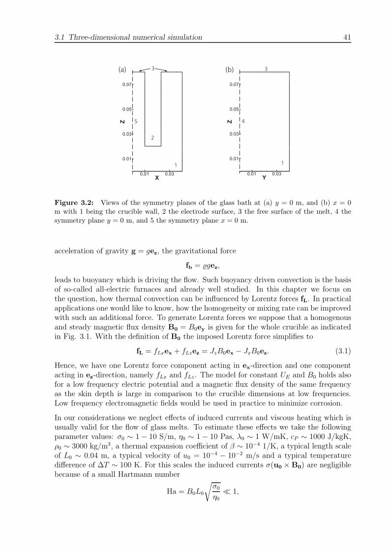
3.1 Three-dimensional numerical simulation 41
Figure 3.2: Views of the symmetry planes of the glass bath at (a) y = 0 m, and (b) x = 0m with 1 being the crucible wall, 2 the electrode surface, 3 the free surface of the melt, 4 thesymmetry plane y = 0 m, and 5 the symmetry plane x = 0 m.
acceleration of gravity g = gez, the gravitational force
fb = gez,
leads to buoyancy which is driving the flow. Such buoyancy driven convection is the basisof so-called all-electric furnaces and already well studied. In this chapter we focus onthe question, how thermal convection can be influenced by Lorentz forces fL. In practicalapplications one would like to know, how the homogeneity or mixing rate can be improvedwith such an additional force. To generate Lorentz forces we suppose that a homogenousand steady magnetic flux density B0 = B0ey is given for the whole crucible as indicatedin Fig. 3.1. With the definition of B0 the imposed Lorentz force simplifies to
fL = fLxex + fLzez = JzB0ex − JxB0ez. (3.1)
Hence, we have one Lorentz force component acting in ex-direction and one componentacting in ez-direction, namely fLx and fLz. The model for constant UE and B0 holds alsofor a low frequency electric potential and a magnetic flux density of the same frequencyas the skin depth is large in comparison to the crucible dimensions at low frequencies.Low frequency electromagnetic fields would be used in practice to minimize corrosion.
In our considerations we neglect effects of induced currents and viscous heating which isusually valid for the flow of glass melts. To estimate these effects we take the followingparameter values: σ0 ∼ 1 − 10 S/m, η0 ∼ 1 − 10 Pas, λ0 ∼ 1 W/mK, cP ∼ 1000 J/kgK,ρ0 ∼ 3000 kg/m3, a thermal expansion coefficient of β ∼ 10−4 1/K, a typical length scaleof L0 ∼ 0.04 m, a typical velocity of u0 = 10−4 − 10−2 m/s and a typical temperaturedifference of ∆T ∼ 100 K. For this scales the induced currents σ(u0 × B0) are negligiblebecause of a small Hartmann number
Ha = B0L0
√σ0
η0≪ 1,

42 3 Electromagnetically controlled flow in a crucible
which describes the ratio between induced electromagnetic force and the friction force[14]. The viscous heating is negligible compared to the heat conduction since the ratio ofboth, the Brinkman number, is
Br =η0u
20
λ0∆T≪ 1.
Furthermore, we do not take into account internal radiative heat transfer as the consideredglass is almost completely non-transparent even for thin layers.
During our studies we only model the glass bath and assume laminar and steady flow.This assumption is valid due to the Rayleigh number Ra of the system, which is
Ra =gβ∆TL3ρ2
0cP
η0λ0
< 105.
The three-dimensional steady flow is governed by the mass conservation equation
∇ · (u) = 0, (3.2)
and the Navier-Stokes equation
∇ · (uu) = −∇p + ∇ ·[η
(∇u + ∇uT
)]+ gez + (Jzex − Jxez)B0, (3.3)
with the following boundary conditions
u = 0 at the electrodes and crucible wall, (3.4)
u · n = 0, ∇(u · t) · n = 0 at the free surface, (3.5)
where n denotes the normal vector, and t the tangential vector of the considered boundaryfaces. The left hand-side of the Navier-Stokes equation (3.3) represents inertia, whereasthe right hand-side represents the body forces. The driving forces are the buoyancy andthe imposed Lorentz force. The velocity boundary conditions are chosen to correspond tothe physical model, i.e. no slip boundary condition at the crucible wall and the electrodes,Eq. (3.4), and free slip boundary condition at the free surface, Eq. (3.5).
The energy equation is solved to determine the temperature T of the melt. With theprescribed assumptions the equation for T is then
cP∇ · (uT ) = ∇ · (λ∇T ) +J2
σ, (3.6)
with the boundary conditions
−(λ∇T ) · n = h(T − T∞) at the crucible wall, (3.7)
−(λ∇T ) · n = ǫσsb(T4 − T 4
∞) at the free surface, (3.8)
(∇T ) · n = 0 at the electrodes, (3.9)
with the ambient temperature T∞, the emissivity ǫ, and the Stefan-Boltzmann constantσsb. The energy equation (3.6) expresses the balance between heat convection on the
3.1 Three-dimensional numerical simulation 43
left hand-side and heat conduction and heat production on the right hand-side. Theheat transfer coefficient h specifies the convective heat transfer at all crucible walls, Eq.(3.7). Under the assumption that h is constant and equal for the whole crucible wall,we evaluated h theoretically. The derivation of h is given in the Appendix A.3. At thefree surface of the melt we assume radiative heat transfer being expressed by the law ofStefan-Boltzmann, Eq. (3.8), where ǫ has to be determined experimentally. The heat flux(∇T ) ·n is assumed to be zero at the electrodes to be consistent with adiabatic conditions.
To calculate the heat input and the imposed Lorentz force we evaluate the Laplace equa-tion for the scalar field of the electric potential φ, which is
∇ · (−σ∇φ) = 0. (3.10)
Eq. (3.10) results from ∇·J = 0 and J = −σ∇φ. The electrodes and the crucible wall aremade of platinum with an electrical conductivity five orders of magnitudes higher thanthat of glass melt. Basically, we can assume that the electrodes and the crucible wall areequipotential surfaces with a constant electric potential, i.e. we define
φ = ±UE/2 at the electrodes, (3.11)
φ = 0 at the crucible wall. (3.12)
For the model the planes x = 0 m and y = 0 m are also the symmetry planes of thephysical model. Firstly, the boundary conditions are applied symmetrically and secondly,the Rayleigh number does not exceed the critical Rayleigh number for symmetry breaking.We verified this assumption with simulations of the whole crucible for various parametersettings. Therefore, we model only a quarter of the glass melt in the crucible. We definethe free slip boundary condition, Eq. (3.5), and the adiabatic boundary condition, Eq.(3.9), at both symmetry planes. If we have φ = −UE/2 at one electrode, φ = UE/2 atthe other electrode, and φ = 0 at the crucible wall, the symmetric electric field gives us
φ = 0 at the plane x=0 m, (3.13)
(∇φ) · n = 0 at the plane y=0 m. (3.14)
An analysis of the governing Eqs. (3.2)-(3.10) shows that the system is highly coupled.Beside the well known coupling of the velocity and the temperature field due to buoyancyin Eq. (3.3) and the heat convection in Eq. (3.6) we have a coupling with the LaplaceEq. (3.10) because of the Lorentz force and the volumetric heat input in Eqs. (3.3) and(3.6), respectively. Overall, the strong variation of the physical properties of the glassmelt leads to a strong coupling as well.
The main focus is to evaluate the governing Eqs. (3.2)-(3.10) and to obtain the unknownsof the system, which are the velocity u and temperature T . We like to obtain an under-standing of the Lorentz force distribution and its effects on the flow. For this purpose wesystematically vary the magnetic flux density B0 and the electric potential difference UE .

44 3 Electromagnetically controlled flow in a crucible
Parameter Value
Heat transfer coefficient h 4 Wm2K
Emissivity ǫ 0.6
Ambient temperature T∞ 1393.15 K
Stefan-Boltzmann constant σsb 5.67 · 10−8 Wm2K4
Table 3.1: Remaining parameter settings. The derivation of h is sketched in the AppendixA.3 and the value of T∞ meets the ambient temperature of the experiment [42].
3.1.2 Implementation and numerical model
The calculations were performed for the glass 3 whose thermophysical properties are givenin Tab. A.2. Glass 3 is characterized by a low viscosity, e.g. η = 1.2 Pas at a temperatureof 1450 K. The composition results in a nearly black glass melt for which the internal heattransfer by radiation is negligible. In Tab. 3.1 the remaining parameters of the presentstudy are summarized.
The coupled set of equations (3.2)-(3.10) has been solved using the commercial softwareFluent which was developed to calculate coupled thermohydrodynamic effects. Further-more, it is possible to solve the transport equation for scalar fields, which we used tosolve the Laplace equation (3.10). With User Defined Functions the Joule heating andthe Lorentz force were calculated and introduced to the Navier-Stokes equation (3.3) andthe Energy equation (3.6).
The discretisation of the governing equations is done by the finite volume method [19].For our calculations we have chosen the implicit method with second-order accuracy. Thepressure and velocity were linked by the Simple algorithm. We have used the defaultsetting for the under-relaxation factors except for the energy equation, which we have setto 0.97 as the strong coupling may led to unintended oscillations if we would have strongtemperature variations. The calculations terminated if the residuals of the continuityand the velocity field were smaller than 10−6 and those of the energy and the scalar fieldwere smaller than 10−9. Furthermore, the convergence has been tested for each set ofparameters by comparing the volumetric heat input with the heat loss over the cruciblewalls and the surface of the melt. If the difference between both was smaller than 10−3
we have assumed convergence, which was the case for all presented results.
The mesh was generated with Gambit and consists of about 6.13 · 105 elements. Thesurface of the melt was meshed using the boundary layer option for the crucible wall andthe electrode. In the remaining area an unstructured face mesh was created which consistsof quadrilateral mesh elements. The mesh node pattern of this source-face was projectedthrough the volume with the Cooper meshing algorithm [20]. We have performed studiesto validate the mesh quality. The mesh study is described in the Appendix A.4. Fig. A.2shows views of the mesh, which was used for all presented calculations.

3.1 Three-dimensional numerical simulation 45
3.1.3 Results
During our simulations we vary the magnetic flux density between −120 mT ≤ B0 ≤120 mT and the electric potential difference between 3 V ≤ UE ≤ 18 V. This is the orderof magnitude of effective magnetic flux densities one can generate for low frequencies asit is used in the laboratory experiment [42]. For the chosen parameter range of UE weare in a thermally stable regime and can perform steady calculations. Larger values ofUE lead to a thermally unstable regime and would require time-dependent calculations.The experimental results presented by Krieger [42] are conducted in a thermally unstableregime. The heat input is kept constant by continuous regulation of UE between 19 Vand 20 V. Therefore, we can not meet the experimental boundary conditions. The steadynumerical simulations presented by Cepite and co-workers [5] reach the temperature rangeof the experiment with UE > 18 V. On the first sight this seems to be a contradiction to thestatement about thermal instability just given. But the physical model of the numericsin [5] contains a rough simplification as the authors define a constant temperature atthe crucible wall. This boundary condition imposes a certain temperature range andavoids thermal instability. But the presented flow pattern looks like the flow in so-calledHedly cells, as the fluid is flowing downwards at all parts of crucible wall. In our opinionthe chosen boundary condition is not correct. In reality the temperature at the wall isnot controlled to a defined value. Instead, the heat transport at the wall is dominated byconvection at the outer surface. Therefore, the direct comparison of the simulation and theexperiment given in [5] is not possible and does not contribute to a better understandingof the physical phenomena in electromagnetically controlled convection of glass melt.
Before we discuss the influence of the Lorentz force on the velocity and temperature fieldlet us have a closer look at the Lorentz force distribution itself.
Lorentz force distribution
Both components of the Lorentz force, fLx = fL · ex and fLz = fL · ez, see Eq. (3.1), canbe rewritten in terms of the electric potential φ and become
fLx = −σ(T )B0∂φ
∂zand fLz = σ(T )B0
∂φ
∂x.
The sign of fLx and fLz – and hence the orientation – can basically be defined by the con-stant magnitude of the magnetic flux density B0 and the gradient of the electric potential∇φ. As the orientation of ∇φ is fixed by the boundary condition at the electrodes, Eq.(3.11), we reverse the direction of fLx and fLz with the sign of B0.
The spatial distribution of the Lorentz force is specified by the temperature-dependentelectrical conductivity σ(T ) and the gradient of the electric potential ∇φ. An example forthe isolines of φ is shown in Fig. 3.3 in the planes y = 0 m and z = 0.04 m. At z ≥ 0.02 mwe mainly find components of ∂φ/∂x (fLz), whereas the intensity of ∂φ/∂z (fLx) is highbelow the electrodes with z < 0.02 m, see Fig. 3.3(a). High values of both Lorentz forcecomponents can be expected around the electrodes due to the very close isolines of φ. Asthe electrical conductivity σ is a function of the temperature, the temperature distribution
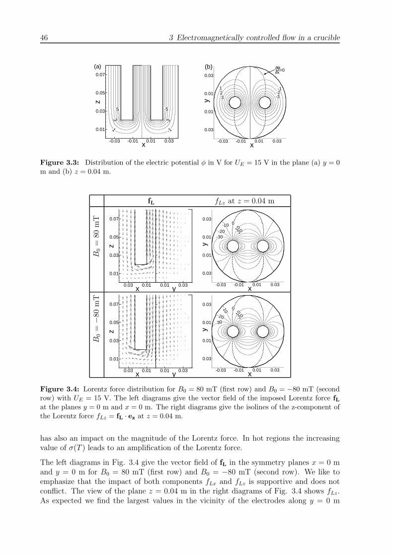
46 3 Electromagnetically controlled flow in a crucible
1
3
5
z
-0.03 -0.01
0.01
0.03
0.05
0.07
(a)
-1
-3
-5
x0.01 0.03 -0.03 -0.01
-0.03
-0.01
x0.01 0.03
123y
0.01
0.03
(b)
-1-2-3
=0φ∂∂x
Figure 3.3: Distribution of the electric potential φ in V for UE = 15 V in the plane (a) y = 0m and (b) z = 0.04 m.
fL fLz at z = 0.04 m
B0
=80
mT
x
z
0.010.03
0.01
0.03
0.05
0.07
y0.01 0.03
1
3
5
7
x0.01 0.03-0.03 -0.01
-0.03
-0.01
-10-20
-3010
20
0
y
0.01
0.03
B0
=−
80m
T
x
z
0.010.03
0.01
0.03
0.05
0.07
y0.01 0.03
1
3
5
7
x0.01 0.03-0.03 -0.01
-0.03
-0.01
10
2030
-10
-20
0
y
0.01
0.03
Figure 3.4: Lorentz force distribution for B0 = 80 mT (first row) and B0 = −80 mT (secondrow) with UE = 15 V. The left diagrams give the vector field of the imposed Lorentz force fLat the planes y = 0 m and x = 0 m. The right diagrams give the isolines of the z-component ofthe Lorentz force fLz = fL · ez at z = 0.04 m.
has also an impact on the magnitude of the Lorentz force. In hot regions the increasingvalue of σ(T ) leads to an amplification of the Lorentz force.
The left diagrams in Fig. 3.4 give the vector field of fL in the symmetry planes x = 0 mand y = 0 m for B0 = 80 mT (first row) and B0 = −80 mT (second row). We like toemphasize that the impact of both components fLx and fLz is supportive and does notconflict. The view of the plane z = 0.04 m in the right diagrams of Fig. 3.4 shows fLz.As expected we find the largest values in the vicinity of the electrodes along y = 0 m
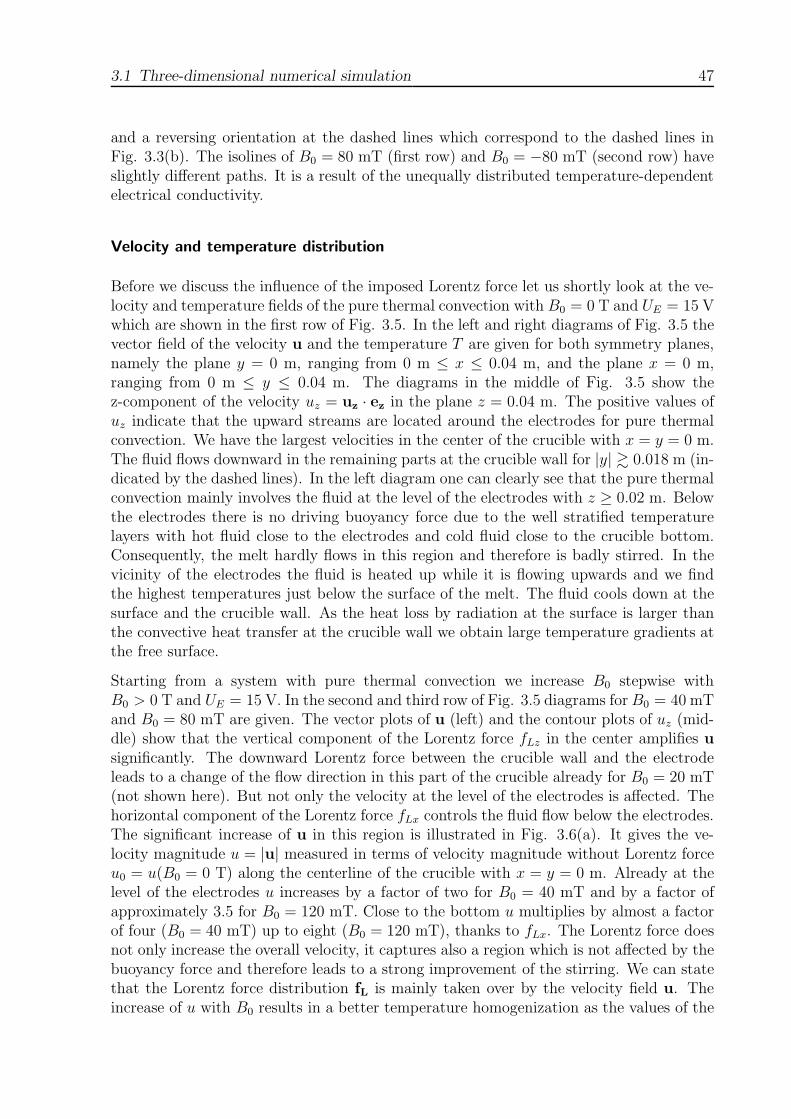
3.1 Three-dimensional numerical simulation 47
and a reversing orientation at the dashed lines which correspond to the dashed lines inFig. 3.3(b). The isolines of B0 = 80 mT (first row) and B0 = −80 mT (second row) haveslightly different paths. It is a result of the unequally distributed temperature-dependentelectrical conductivity.
Velocity and temperature distribution
Before we discuss the influence of the imposed Lorentz force let us shortly look at the ve-locity and temperature fields of the pure thermal convection with B0 = 0 T and UE = 15 Vwhich are shown in the first row of Fig. 3.5. In the left and right diagrams of Fig. 3.5 thevector field of the velocity u and the temperature T are given for both symmetry planes,namely the plane y = 0 m, ranging from 0 m ≤ x ≤ 0.04 m, and the plane x = 0 m,ranging from 0 m ≤ y ≤ 0.04 m. The diagrams in the middle of Fig. 3.5 show thez-component of the velocity uz = uz · ez in the plane z = 0.04 m. The positive values ofuz indicate that the upward streams are located around the electrodes for pure thermalconvection. We have the largest velocities in the center of the crucible with x = y = 0 m.The fluid flows downward in the remaining parts at the crucible wall for |y| & 0.018 m (in-dicated by the dashed lines). In the left diagram one can clearly see that the pure thermalconvection mainly involves the fluid at the level of the electrodes with z ≥ 0.02 m. Belowthe electrodes there is no driving buoyancy force due to the well stratified temperaturelayers with hot fluid close to the electrodes and cold fluid close to the crucible bottom.Consequently, the melt hardly flows in this region and therefore is badly stirred. In thevicinity of the electrodes the fluid is heated up while it is flowing upwards and we findthe highest temperatures just below the surface of the melt. The fluid cools down at thesurface and the crucible wall. As the heat loss by radiation at the surface is larger thanthe convective heat transfer at the crucible wall we obtain large temperature gradients atthe free surface.
Starting from a system with pure thermal convection we increase B0 stepwise withB0 > 0 T and UE = 15 V. In the second and third row of Fig. 3.5 diagrams for B0 = 40 mTand B0 = 80 mT are given. The vector plots of u (left) and the contour plots of uz (mid-dle) show that the vertical component of the Lorentz force fLz in the center amplifies u
significantly. The downward Lorentz force between the crucible wall and the electrodeleads to a change of the flow direction in this part of the crucible already for B0 = 20 mT(not shown here). But not only the velocity at the level of the electrodes is affected. Thehorizontal component of the Lorentz force fLx controls the fluid flow below the electrodes.The significant increase of u in this region is illustrated in Fig. 3.6(a). It gives the ve-locity magnitude u = |u| measured in terms of velocity magnitude without Lorentz forceu0 = u(B0 = 0 T) along the centerline of the crucible with x = y = 0 m. Already at thelevel of the electrodes u increases by a factor of two for B0 = 40 mT and by a factor ofapproximately 3.5 for B0 = 120 mT. Close to the bottom u multiplies by almost a factorof four (B0 = 40 mT) up to eight (B0 = 120 mT), thanks to fLx. The Lorentz force doesnot only increase the overall velocity, it captures also a region which is not affected by thebuoyancy force and therefore leads to a strong improvement of the stirring. We can statethat the Lorentz force distribution fL is mainly taken over by the velocity field u. Theincrease of u with B0 results in a better temperature homogenization as the values of the

48 3 Electromagnetically controlled flow in a crucible
u uz T
B0
=0
T
x
z
0.010.03
0.01
0.03
0.05
0.07
y0.01 0.03
1
3
5
7
-0.03 -0.01
-0.03
-0.01
x0.01 0.03
-0.2-0.4
0.2
0.2
0.40.6
0
y
0.01
0.03
1444
1440
y0.01 0.03
1
3
5
7
1448
x
z
0.010.03
0.01
0.03
0.05
0.07
B0
=40
mT
x
z
0.010.03
0.01
0.03
0.05
0.07
y0.01 0.03
1
3
5
7
x0.01 0.03-0.03 -0.01
-0.03
-0.01
-0.4
0.4
1.20.8
-0.4
0
y
0.01
0.03
y0.01 0.03
1
3
5
7
1440
1444
xz
0.010.03
0.01
0.03
0.05
0.07
B0
=80
mT
x
z
0.010.03
0.01
0.03
0.05
0.07
y0.01 0.03
1
3
5
7
-0.4
-0.8
0.4
1.2
2.0
0
y
0.01
0.03
-0.03 -0.01
-0.03
-0.01
x0.01 0.03
1440
x
z
0.010.03
0.01
0.03
0.05
0.07
1436
y0.01 0.03
1
3
5
7
Figure 3.5: The vector field of the velocity u (left), isolines of the z-component uz = u · ez
in mm/s (middle) and the temperature T in K (right) for B0 = 0 T, B0 = 40 mT, B0 = 80mT (starting from the first row) and UE = 15 V. The velocity field u and the temperature Tare shown for both symmetry planes, namely the plane y = 0 m and the plane x = 0 m. Thez-component of the velocity uz is plotted in the plane z = 0.04 m. The region with the largesttemperature, so-called hot spots, are highlighted in grey.
highest temperature decrease. Fig. 3.6(b) illustrates the temperature homogenization onthe basis of the temperature along x = y = 0 m. A similar temperature homogenizationfor B0 > 0 T was observed experimentally by Krieger [42]. The results differ only in thetemperature range due to the different heat inputs.
In the following we reverse the direction of the magnetic field and decrease the magneticfield stepwise starting again from B0 = 0 T. First let us look at cases with B0 = −40 mTand B0 = −70 mT which are shown in the second and third row in Fig. 3.7. Now thevertical component of the Lorentz force fLz supports the thermally driven upward flowbetween the crucible wall and the electrodes as uz increases, compare uz for B0 = 0 T withuz for B0 = −40 mT and B0 = −70 mT in Fig. 3.7. Again, fLx controls the flow below the

3.1 Three-dimensional numerical simulation 49
0 2 4 6 8
0.01
0.03
0.05
0.07
u/u0
z [m
]
B0=20 mT
B0=40 mT
B0=60 mT
B0=80 mT
B0=100 mT
B0=120 mT
(a)
1430 1435 1440 1445 1450 1455
0.01
0.03
0.05
0.07
T [K]
z [m
]
B0=0 mT
B0=20 mT
B0=40 mT
B0=60 mT
B0=80 mT
B0=100 mT
B0=120 mT
(b)
Figure 3.6: (a) The velocity ratio u/u0 gives the proportion of the velocity magnitude u = |u|with Lorentz force for B0 > 0 T in comparison to that without Lorentz force u0 = u(B0 = 0T)in the centerline of the crucible (x = y = 0 m) and UE = 15 V corresponding to Fig. 3.5. Thedashed line gives u = u0. In (b) the corresponding temperature distribution is shown.
electrodes. Between the electrodes the downward acting Lorentz force does not lead to anabrupt overall change of the flow direction. At the upper half level of the electrodes uz isstill positive. But the magnitude of the velocity is reduced significantly compared to thethermally driven flow with B0 = 0 T (first row in Fig. 3.7). The upward stream is drivenby buoyancy due to the large temperature gradients just below the surface. Just the fluidbelow z ≈ 0.03 m (B0 = −70 mT) flows downward with a very small magnitude drivenby the Lorentz force. However, the small magnitudes of the velocity are an indicator foralmost equal forces – nether the buoyancy nor the Lorentz force is clearly dominating inthe center of the crucible. As a result, the region of the almost stagnant flow regime closeto the bottom of the center expands. On the one hand fL leads to a better motion belowthe electrodes and larger velocities at the crucible wall. On the other hand the motionbetween the electrodes slows down and leads to an almost stagnant flow region. Fig.3.8(a) shows the reduction of u in the centerline for B0 = −20 mT, −40 mT, and −60mT in comparison to u0 = u(B0 = 0 T). Especially for z ≤ 0.03 m u reduces dramaticallyand tends to zero. Due to the low velocities in the centerline the temperatures betweenthe electrodes and the temperature differences increase significantly as it is shown in Fig.3.8(b).
If we now slightly change the magnetic flux density from B0 = −70 mT to B0 = −71 mTwe observe a drastic change in the flow pattern and temperature distribution, comparethird and forth row of Fig. 3.7. In the centerline buoyancy can not compensate fLz
which leads to a change of flow direction with large changes of the velocity magnitude.Now the fluid in the vicinity of the centerline is flowing downwards, moving below theelectrodes to the crucible wall and between the crucible wall and the electrode to thesurface. The velocity magnitude in the center, especially for z < 0.03 m, is now againa multiple of the velocity magnitude without Lorentz forces as indicated by the curveswith B0 = −80mT,−100mT,−120mT in Fig. 3.8(a). For B0 ≤ −71 mT the qualitativepicture of the velocity field u corresponds to the distribution of the Lorentz force fL and

50 3 Electromagnetically controlled flow in a crucible
u uz T
B0
=0
T
x
z
0.010.03
0.01
0.03
0.05
0.07
y0.01 0.03
1
3
5
7
-0.03 -0.01
-0.03
-0.01
x0.01 0.03
-0.2-0.4
0.2
0.2
0.40.6
0
y
0.01
0.03
1444
1440
y0.01 0.03
1
3
5
7
1448
x
z
0.010.03
0.01
0.03
0.05
0.07
B0
=−
40m
T
x
z
0.010.03
0.01
0.03
0.05
0.07
y0.01 0.03
1
3
5
7
x0.01 0.03-0.03 -0.01
-0.03
-0.01
-0.4-0.2
0.20.4
0.20.60
y
0.01
0.03
1452
y0.01 0.03
1
3
5
7
1456
xz
0.010.03
0.01
0.03
0.05
0.07
B0
=−
70m
T
x
z
0.010.03
0.01
0.03
0.05
0.07
y0.01 0.03
1
3
5
7 -0.8-0.4
0.4
0.8
0
y
0.01
0.03
x0.01 0.03-0.03 -0.01
-0.03
-0.0114
64
y0.01 0.03
1
3
5
7
1468
x
z
0.010.03
0.01
0.03
0.05
0.07
B0
=−
71m
T
x
z
0.010.03
0.01
0.03
0.05
0.07
y0.01 0.03
1
3
5
7
x0.01 0.03-0.03 -0.01
-0.03
-0.01
-0.4 -0.80.4
0.8
1.2
-1.2
0
y
0.01
0.03
y0.01 0.03
1
3
5
7
14481444
x
z
0.010.03
0.01
0.03
0.05
0.07
Figure 3.7: The vector field of the velocity u (left), isolines of the z-component uz = u · ez
in mm/s (middle) and the temperature T in K (right) for B0 = 0 T, B0 = −40 mT, B0 = −70mT, B0 = −71 mT (starting from the first row) and UE = 15 V. The results are obtained bystarting from a system with B0 = 0 T and reducing B0 stepwise. Always a converged solutionis used as starting condition for the calculation.
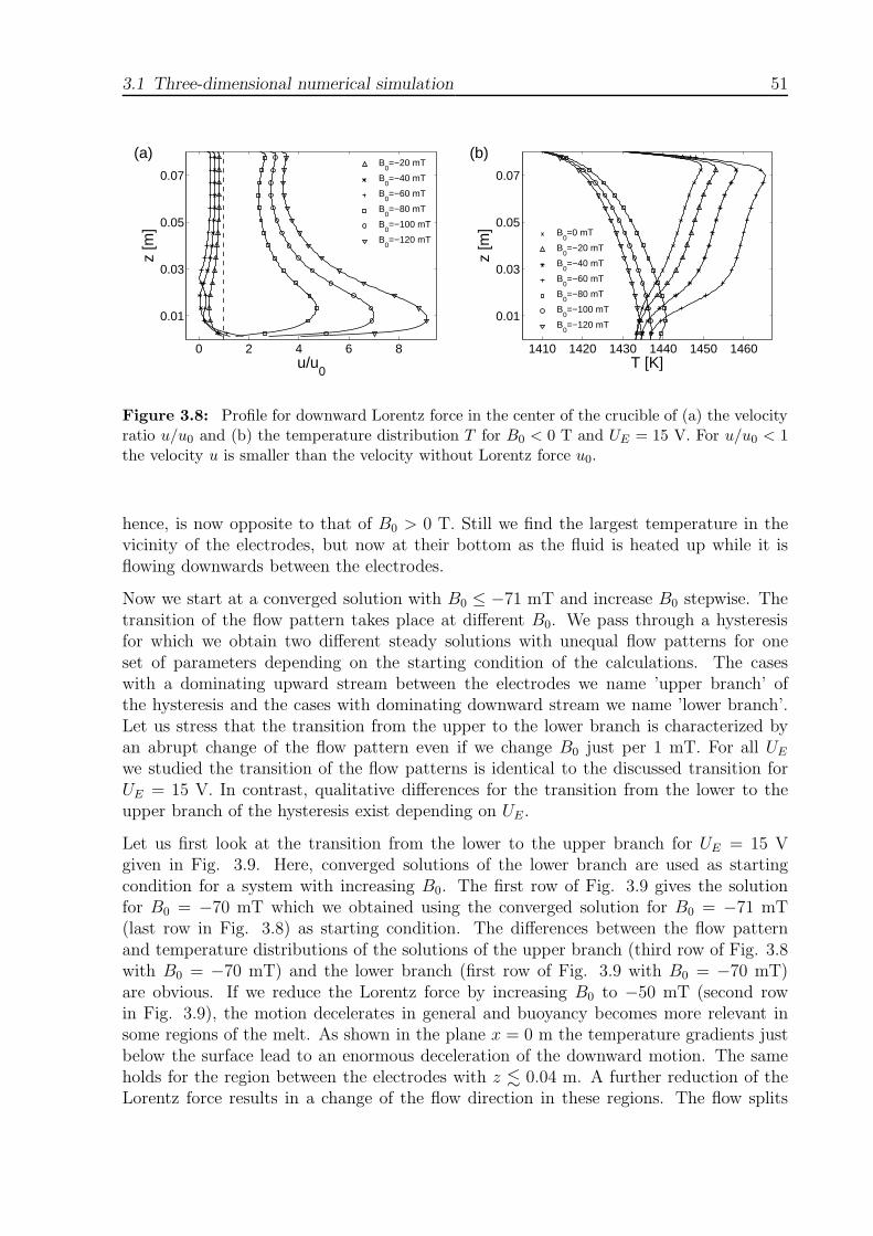
3.1 Three-dimensional numerical simulation 51
0 2 4 6 8
0.01
0.03
0.05
0.07
u/u0
z [m
]
B0=−20 mT
B0=−40 mT
B0=−60 mT
B0=−80 mT
B0=−100 mT
B0=−120 mT
(a)
1410 1420 1430 1440 1450 1460
0.01
0.03
0.05
0.07
T [K]
z [m
]
B0=0 mT
B0=−20 mT
B0=−40 mT
B0=−60 mT
B0=−80 mT
B0=−100 mT
B0=−120 mT
(b)
Figure 3.8: Profile for downward Lorentz force in the center of the crucible of (a) the velocityratio u/u0 and (b) the temperature distribution T for B0 < 0 T and UE = 15 V. For u/u0 < 1the velocity u is smaller than the velocity without Lorentz force u0.
hence, is now opposite to that of B0 > 0 T. Still we find the largest temperature in thevicinity of the electrodes, but now at their bottom as the fluid is heated up while it isflowing downwards between the electrodes.
Now we start at a converged solution with B0 ≤ −71 mT and increase B0 stepwise. Thetransition of the flow pattern takes place at different B0. We pass through a hysteresisfor which we obtain two different steady solutions with unequal flow patterns for oneset of parameters depending on the starting condition of the calculations. The caseswith a dominating upward stream between the electrodes we name ’upper branch’ ofthe hysteresis and the cases with dominating downward stream we name ’lower branch’.Let us stress that the transition from the upper to the lower branch is characterized byan abrupt change of the flow pattern even if we change B0 just per 1 mT. For all UE
we studied the transition of the flow patterns is identical to the discussed transition forUE = 15 V. In contrast, qualitative differences for the transition from the lower to theupper branch of the hysteresis exist depending on UE .
Let us first look at the transition from the lower to the upper branch for UE = 15 Vgiven in Fig. 3.9. Here, converged solutions of the lower branch are used as startingcondition for a system with increasing B0. The first row of Fig. 3.9 gives the solutionfor B0 = −70 mT which we obtained using the converged solution for B0 = −71 mT(last row in Fig. 3.8) as starting condition. The differences between the flow patternand temperature distributions of the solutions of the upper branch (third row of Fig. 3.8with B0 = −70 mT) and the lower branch (first row of Fig. 3.9 with B0 = −70 mT)are obvious. If we reduce the Lorentz force by increasing B0 to −50 mT (second rowin Fig. 3.9), the motion decelerates in general and buoyancy becomes more relevant insome regions of the melt. As shown in the plane x = 0 m the temperature gradients justbelow the surface lead to an enormous deceleration of the downward motion. The sameholds for the region between the electrodes with z . 0.04 m. A further reduction of theLorentz force results in a change of the flow direction in these regions. The flow splits
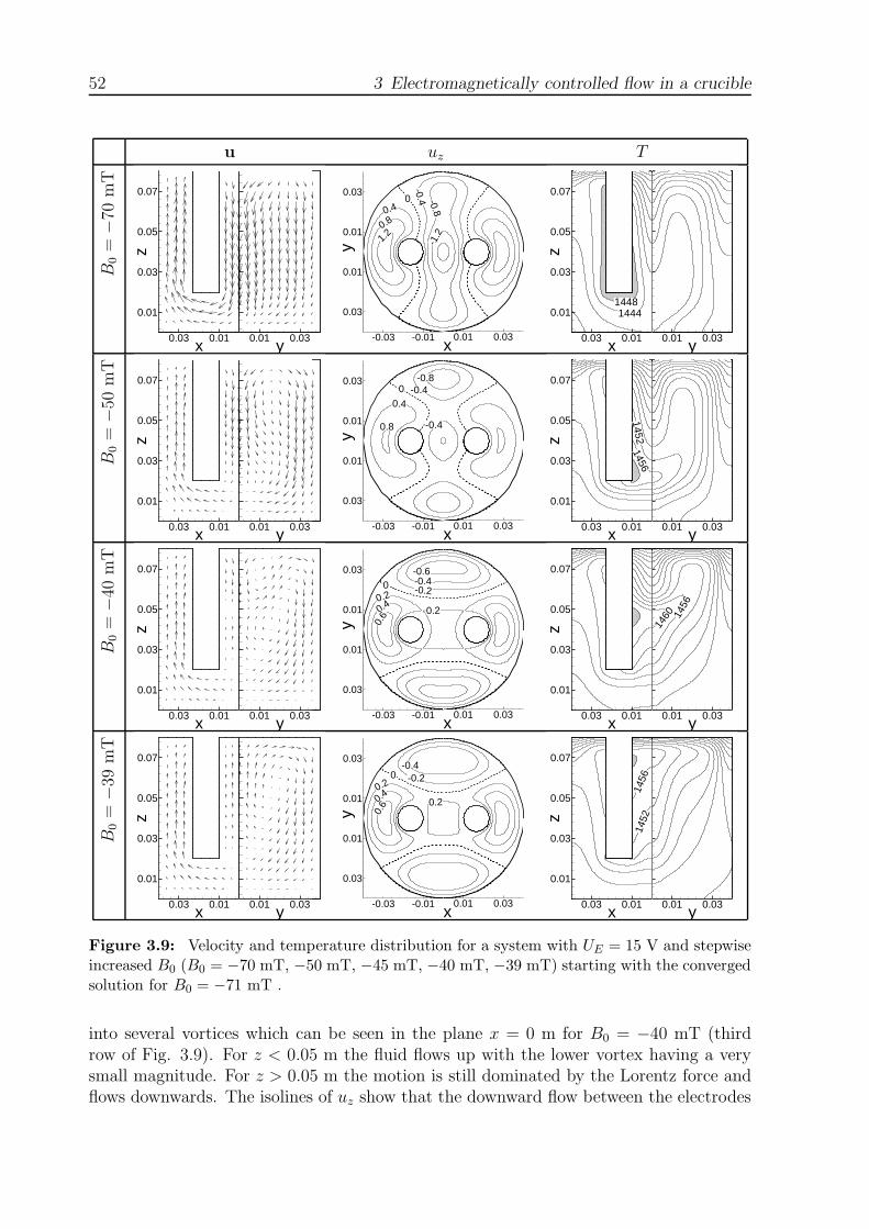
52 3 Electromagnetically controlled flow in a crucible
u uz T
B0
=−
70m
T
x
z
0.010.03
0.01
0.03
0.05
0.07
y0.01 0.03
1
3
5
7
-0.03 -0.01
-0.03
-0.01
x0.01 0.03
0.4
0.8
1.2
-0.4 -0.8-1
.2
0
y
0.01
0.03
y0.01 0.03
1
3
5
7
14441448
x
z
0.010.03
0.01
0.03
0.05
0.07
B0
=−
50m
T
x
z
0.010.03
0.01
0.03
0.05
0.07
y0.01 0.03
1
3
5
7
-0.4-0.8
0.4
0.8 -0.4
0
y
0.01
0.03
x0.01 0.03-0.03 -0.01
-0.03
-0.01
y0.01 0.03
1
3
5
7
14561452
xz
0.010.03
0.01
0.03
0.05
0.07
B0
=−
40m
T
x
z
0.010.03
0.01
0.03
0.05
0.07
y0.01 0.03
1
3
5
7
x0.01 0.03-0.03 -0.01
-0.03
-0.01
-0.6-0.4-0.2
0.20.4
0.6 0.2
0
y
0.01
0.03
1460 14
56
y0.01 0.03
1
3
5
7
x
z
0.010.03
0.01
0.03
0.05
0.07
B0
=−
39m
T
y0.01 0.03
1
3
5
7
x
z
0.010.03
0.01
0.03
0.05
0.07
x0.01 0.03-0.03 -0.01
-0.03
-0.01
-0.2-0.4
0.2
0.4
0.6 0.2
0
y
0.01
0.03
y0.01 0.03
1
3
5
7
1456
1452
x
z
0.010.03
0.01
0.03
0.05
0.07
Figure 3.9: Velocity and temperature distribution for a system with UE = 15 V and stepwiseincreased B0 (B0 = −70 mT, −50 mT, −45 mT, −40 mT, −39 mT) starting with the convergedsolution for B0 = −71 mT .
into several vortices which can be seen in the plane x = 0 m for B0 = −40 mT (thirdrow of Fig. 3.9). For z < 0.05 m the fluid flows up with the lower vortex having a verysmall magnitude. For z > 0.05 m the motion is still dominated by the Lorentz force andflows downwards. The isolines of uz show that the downward flow between the electrodes

3.1 Three-dimensional numerical simulation 53
u uz TB
0=
−46
mT
y0.01 0.03
1
3
5
7
x
z
0.010.03
0.01
0.03
0.05
0.07
x0.01 0.03-0.03 -0.01
-0.03
-0.01
-0.6
-0.4
-0.2
0.20.4
0
y
0.01
0.03
x
z
0.010.03
0.01
0.03
0.05
0.07
14281424
y0.01 0.03
1
3
5
7
B0
=−
45m
T
x
z
0.010.03
0.01
0.03
0.05
0.07
y0.01 0.03
1
3
5
7
x0.01 0.03-0.03 -0.01
-0.03
-0.01
-0.4
-0.2
0.2
0.40.2
0y
0.01
0.03
1428
1424
y0.01 0.03
1
3
5
7
x
z
0.010.03
0.01
0.03
0.05
0.07
Figure 3.10: Velocity and temperature distribution showing the transition from the lower tothe upper branch for UE = 12 V.
is limited to a small region (bounded by the dashed lines). But in the centerline thevelocity magnitude of the downward flow is still larger than the magnitude of the upwardflow. While we increase B0 from −70 mT up to −40 mT the hot spot in the vicinity ofthe electrodes moves from the bottom of the electrodes (B0 = −70 mT) to the regionbetween the electrodes. There, the hot spot is moving from z ≈ 0.023 m (B0 = −50 mT)to z ≈ 0.048 m (B0 = −40 mT). The downward stream between the electrodes disappearscompletely for B0 = −39 mT as shown in the last row of Fig. 3.9. Thus, the transitionfrom the lower to the upper branch is characterized by the merging of the two vortices toa single vortex in the centerline.
Fig. 3.10 illustrates the transition from the lower to the upper branch for UE = 12 V. Justbefore the transition, B0 = −46 mT, buoyancy leads to a reversing of the flow directiononly in the centerline with z ≤ 0.032 m. The temperature gradient below the surface doesnot lead to upward streams and hence, the flow does not split into several vortices.
One possibility to illustrate the regime of the two-valued solutions and the transition ofthe flow pattern is to look at the maximum z-component of the velocity at x = y = 0 m,which we label uzmax. The transition of the flow pattern is characterized by a shift of thesign of uzmax, whereas uzmax is greater than zero at the upper branch and smaller thanzero at the lower branch. In Fig. 3.11(a) uzmax is given as a function of B0 for variousUE . The right diagram gives a detailed view of the region with two solutions. First ofall, the region of two-valued solutions uzmax(B0) depends on UE . As summarized in Tab.3.2 we obtain two solutions between −58 mT ≤ B0 ≤ −46 mT for UE = 9 V. This rangeexpands to −71 mT ≤ B0 ≤ −46 mT if we consider UE = 12 V. A further increase of

54 3 Electromagnetically controlled flow in a crucible
−0.1 −0.05 0 0.05 0.1−8
−6
−4
−2
0
2
4
6
8
B0 [T]
u zmax
[mm
/s] a
t x=
y=0
m
UE=9 V
UE=12 V
UE=15 V
UE=18 V
(a)
−0.06 −0.04−5
−4
−3
−2
−1
0
1
B0 [T]
u zmax
[mm
/s] a
t x=
y=0
m
−0.1 −0.05 0 0.05 0.1−6
−4
−2
0
2
4
6
B0 [T]
u zmax
/uzm
ax,0
at x
=y=
0 m
UE=9 V
UE=12 V
UE=15 V
UE=18 V
(b)
−0.06 −0.04
−3
−2
−1
0
1
B0 [T]
u zmax
/uzm
ax,0
at x
=y=
0 m
Figure 3.11: (a) Maximum z-velocity of the velocity in the centerline of the crucible uzmax asa function of B0 for various UE. In (b) the ratio between uzmax and uzmax,0 = uzmax(B0 = 0T) is given. The detailed views (right) show that the range of two-valued solutions uzmax(B0)depends significantly on UE .
UE B0
Range of two-valued solution
9 V -46 mT ... -58 mT
12 V -46 mT ... -71 mT
15 V -40 mT ... -70 mT
18 V -27 mT ... -56 mT
Table 3.2: Range of magnetic flux densities B0 for which we obtain two different solutionsdepending on the starting conditions of the calculations. The range of B0 varies with the electricpotential difference UE .
the electric potential difference to UE = 15 V leads only to a similar parameter rangeof two solutions, which is −70 mT ≤ B0 ≤ −40 mT. For UE = 18 V the change fromuzmax > 0 to uzmax < 0 happens if we start at a steady solution with B0 = −56 mT andapply B0 = −57 mT. Therefore, the parameter range with two steady solutions changesto −56 mT ≤ B0 ≤ −27 mT. In Fig. 3.11(b) uzmax is measured in terms of the maximum

3.1 Three-dimensional numerical simulation 55
z-component of the velocity without Lorentz force, uzmax,0 = uzmax(B0 = 0). The diagramuzmax/uzmax,0(B0) confirms that the velocity increases almost linearly with B0 for B0 > 0T. The deceleration of the motion in the upper branch with B0 < 0 T is reflected in Fig.3.11(b) as 0 < uzmax/uzmax,0 < 1.
Maximum stretching function
For the application not only the effects of the Lorentz force on the temperature distributionand velocity field are important. Especially the effect on the homogenization – how themixing in laminar flow can be improved – is of interest. Laminar mixing is characterizedby molecular diffusion on the interfaces between two fluids or inhomogeneities. It isbased on the interface increase by deformation of fluid volumes. Different definitions existto quantify the mixing effect [59]. Typically deformations of infinitesimal elements, lines,surfaces, and volumes are used which are based on the stretching function. The stretchingfunction is a measure of the deformation velocity of an element. Its theoretical maximumvalue α is given by [68]
α =√
D : D, (3.15)
where D = 1/2(∇u + (∇u)T ) is the symmetric stretching tensor. As pure rotation doesnot contribute to the deformation of fluid volumes the antisymmetric vorticity tensor isnot part of the definition of α. α can be obtained easily from the presented simulationdata of the velocity field. Large α lead to large deformations and an increase of theinterface between the fluid volumes. The goal of each mixing techniques is to maximizethe deformation and hence, to maximize α in the whole volume. It is a first step towardsthe evaluation of the influence of the Lorentz force on laminar mixing.
Fig. 3.12 shows isolines of α for pure thermal convection (first row) and for Lorentzforce dominated flows with B0 = 80 mT (second row) and B0 = −80 mT (third row).Due to low velocities below the electrodes and close to the bottom for B0 = 0 T, α isvery small in this region as indicated by the grey shaded areas. We find larger valuesof α around the electrodes and for y ≥ 0.035 m in the plane x = 0 m because of theadditional isolines. In Lorentz force dominated regimes (second and third row of Fig.3.12) α increases significantly as the grey shaded areas almost disappear, especially closeto the bottom for z ≤ 0.02 m. We can observe some differences in the α distributionfor B0 = 80 mT and B0 = −80 mT even though the magnitudes of both magnetic fluxdensities are equal and the flow is dominated by the Lorentz force. For B0 = 80 mT αhardly changes for y ≥ 0.025 m. But for B0 = −80 mT we observe a slight increase of αin this region due to closer isolines. We find the largest values of α in the vicinity of theelectrodes for both signs of B0. In the case of B0 = 80 mT the isoline density is largestbetween the electrodes. In contrast, the isoline density is largest between the cruciblewall and one electrode for B0 = −80 mT.
Slight differences also exist between the solutions of the upper and the lower branch ofthe two-valued regime which are obtained with the same set of parameters. As shown inFig. 3.13 for B0 = −40 mT α differs in the region between the electrodes. Due to thesplit of the flow in vortices α is larger for the solutions of the lower branch (second row

56 3 Electromagnetically controlled flow in a crucible
B0
=0
T
x
z
0.010.03
0.01
0.03
0.05
0.07
y0.01 0.03
1
3
5
7
y
0.01
0.03
x0.01 0.03-0.03 -0.01
-0.03
-0.01
B0
=80
mT
y0.01 0.03
1
3
5
7
x
z
0.010.03
0.01
0.03
0.05
0.07
y
0.01
0.03
-0.03 -0.01
-0.03
-0.01
x0.01 0.03
B0
=−
80m
T
x
z
0.010.03
0.01
0.03
0.05
0.07
y0.01 0.03
1
3
5
7
y
0.01
0.03
x0.01 0.03-0.03 -0.01
-0.03
-0.01
Figure 3.12: Isolines of the maximum stretching function α in s−1 in the planes y = 0 m,x = 0 m (left) and z = 0.04 m (right) for UE = 15 V. In the first row α is given for pure thermalconvection. The second (B0 = 80 mT) and third row (B0 = −80 mT) show α for Lorentz forcedominated flows. The grey shading highlights areas with α ≤ 0.02 s−1. Between the isolines thedifference of α is 0.04 s−1.
in Fig. 3.13) than for the solutions of the upper branch (first row in Fig. 3.13) of thehysteresis.
Global analysis
During the discussions in the previous section we gained a good insight into the electro-magnetically flow control by studying flow pattern, temperature distributions, variationsof local velocities and temperatures, and the distribution of the maximum stretching func-tion. In the following paragraphs a coarse measure of the overall influence of the imposedLorentz force on the flow can be given with volume-averaged quantities.
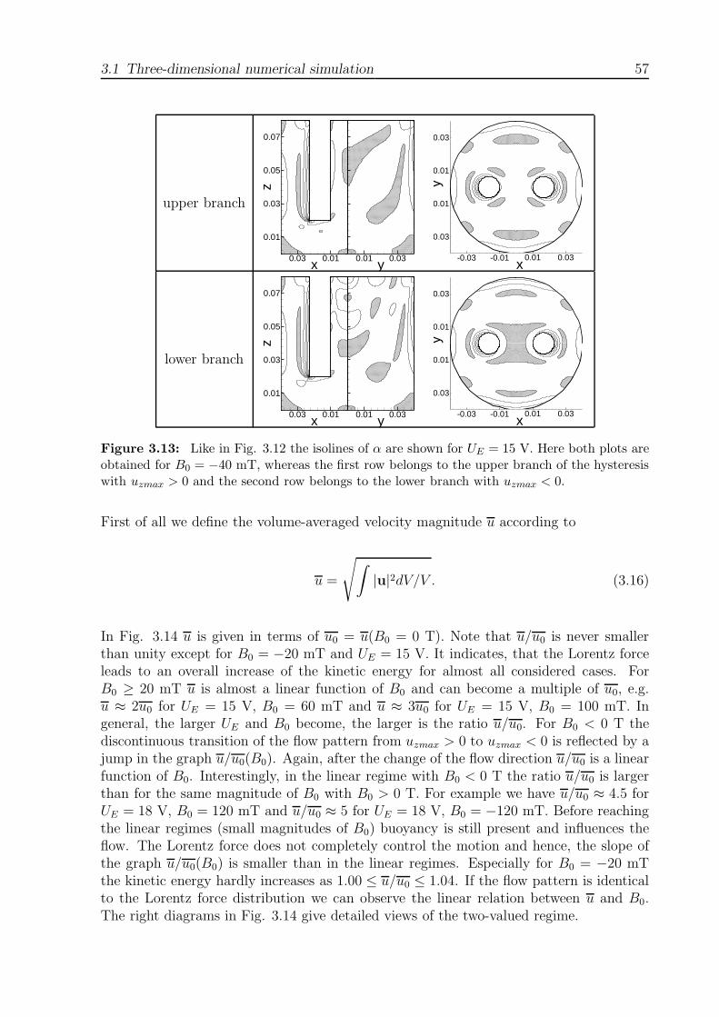
3.1 Three-dimensional numerical simulation 57
upper branch
xz
0.010.03
0.01
0.03
0.05
0.07
y0.01 0.03
1
3
5
7
y
0.01
0.03
x0.01 0.03-0.03 -0.01
-0.03
-0.01
lower branch
x
z
0.010.03
0.01
0.03
0.05
0.07
y0.01 0.03
1
3
5
7
y
0.01
0.03
x0.01 0.03-0.03 -0.01
-0.03
-0.01
Figure 3.13: Like in Fig. 3.12 the isolines of α are shown for UE = 15 V. Here both plots areobtained for B0 = −40 mT, whereas the first row belongs to the upper branch of the hysteresiswith uzmax > 0 and the second row belongs to the lower branch with uzmax < 0.
First of all we define the volume-averaged velocity magnitude u according to
u =
√∫|u|2dV/V . (3.16)
In Fig. 3.14 u is given in terms of u0 = u(B0 = 0 T). Note that u/u0 is never smallerthan unity except for B0 = −20 mT and UE = 15 V. It indicates, that the Lorentz forceleads to an overall increase of the kinetic energy for almost all considered cases. ForB0 ≥ 20 mT u is almost a linear function of B0 and can become a multiple of u0, e.g.u ≈ 2u0 for UE = 15 V, B0 = 60 mT and u ≈ 3u0 for UE = 15 V, B0 = 100 mT. Ingeneral, the larger UE and B0 become, the larger is the ratio u/u0. For B0 < 0 T thediscontinuous transition of the flow pattern from uzmax > 0 to uzmax < 0 is reflected by ajump in the graph u/u0(B0). Again, after the change of the flow direction u/u0 is a linearfunction of B0. Interestingly, in the linear regime with B0 < 0 T the ratio u/u0 is largerthan for the same magnitude of B0 with B0 > 0 T. For example we have u/u0 ≈ 4.5 forUE = 18 V, B0 = 120 mT and u/u0 ≈ 5 for UE = 18 V, B0 = −120 mT. Before reachingthe linear regimes (small magnitudes of B0) buoyancy is still present and influences theflow. The Lorentz force does not completely control the motion and hence, the slope ofthe graph u/u0(B0) is smaller than in the linear regimes. Especially for B0 = −20 mTthe kinetic energy hardly increases as 1.00 ≤ u/u0 ≤ 1.04. If the flow pattern is identicalto the Lorentz force distribution we can observe the linear relation between u and B0.The right diagrams in Fig. 3.14 give detailed views of the two-valued regime.
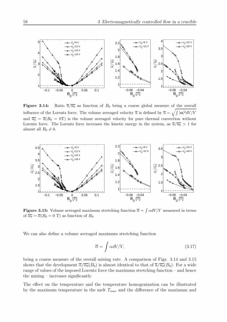
58 3 Electromagnetically controlled flow in a crucible
−0.1 −0.05 0 0.05 0.11
2
3
4
5
B0 [T]
u/u0
UE=9 V
UE=12 V
UE=15 V
UE=18 V
−0.06 −0.04
1
1.2
1.4
1.6
1.8
2
2.2
B0 [T]
u/u0
UE=9 V
UE=12 V
−0.06 −0.041
1.5
2
2.5
3
3.5
4
B0 [T]
u/u0
UE=15 V
UE=18 V
Figure 3.14: Ratio u/u0 as function of B0 being a coarse global measure of the overall
influence of the Lorentz force. The volume averaged velocity u is defined by u =√∫
|u|2dV/V
and u0 = u(B0 = 0T) is the volume averaged velocity for pure thermal convection withoutLorentz force. The Lorentz force increases the kinetic energy in the system, as u/u0 > 1 foralmost all B0 6= 0.
−0.1 −0.05 0 0.05 0.11
1.5
2
2.5
3
3.5
4
4.5
B0 [T]
α/α
0
UE=9 V
UE=12 V
UE=15 V
UE=18 V
−0.06 −0.04
1
1.2
1.4
1.6
1.8
2
2.2
B0 [T]
α/α
0
UE=9 V
UE=12 V
−0.06 −0.041
1.5
2
2.5
3
3.5
B0 [T]
α/α
0
UE=15 V
UE=18 V
Figure 3.15: Volume averaged maximum stretching function α =∫
αdV/V measured in termsof α0 = α(B0 = 0 T) as function of B0.
We can also define a volume averaged maximum stretching function
α =
∫αdV/V, (3.17)
being a coarse measure of the overall mixing rate. A comparison of Figs. 3.14 and 3.15shows that the development α/α0(B0) is almost identical to that of u/u0(B0). For a widerange of values of the imposed Lorentz force the maximum stretching function – and hencethe mixing – increases significantly.
The effect on the temperature and the temperature homogenization can be illustratedby the maximum temperature in the melt Tmax and the difference of the maximum and

3.1 Three-dimensional numerical simulation 59
−0.1 −0.05 0 0.05 0.11400
1450
1500
1550
B0 [T]
Tm
ax [K
]
UE=9 V
UE=12 V
UE=15 V
UE=18 V
(a)
−0.1 −0.05 0 0.05 0.1
0.8
1
1.2
1.4
1.6
1.8
B0 [T]
∆T/∆
T0
UE=9 V
UE=12 V
UE=15 V
UE=18 V
(b)
−0.06 −0.040.9
1
1.1
1.2
1.3
1.4
B0 [T]
∆T/∆
T0
UE=9 V
UE=12 V
−0.06 −0.04
1
1.2
1.4
1.6
1.8
2
B0 [T]
∆T/∆
T0
UE=15 V
UE=18 V
Figure 3.16: (a) The maximum temperature in the melt Tmax as function of B0. In (b) theratio of the temperature difference ∆T = Tmax−Tmin and the temperature difference of the purethermal convection ∆T0 = ∆T (B0 = 0 T) is given. The temperature homogenization improveswith B0 if ∆T/∆T0 < 1 and changes to the worse for ∆T/∆T0 > 1.
minimum temperature in the melt
∆T = Tmax − Tmin. (3.18)
In Fig. 3.16(a) Tmax(B0) and in Fig. 3.16(b) ∆T/∆T0(B0) with ∆T0 = ∆T (B0 = 0 T) aregiven. For B0 > 0 T and all UE we have ∆T/∆T0 < 1 – the temperature homogenizationimproves. The smaller UE the smaller ∆T/∆T0 becomes. If we look at B0 < 0 T anddecrease B0 starting from B0 = 0 T we observe that ∆T/∆T0 significantly increases. Itindicates a worse temperature homogenization than without Lorentz force. For UE = 9 Vwe have a maximum of ∆T/∆T0 ≈ 1.22, but if we double UE the maximum temperaturedifference in the melt is ∆T/∆T0 ≈ 1.73 which is reached just before the change of flowdirection. Also the transition from the lower to the upper branch of the hysteresis ischaracterized by ∆T/∆T0 > 1.
Finally, let us have a look at the overall volume-averaged Lorentz force
fL = V −1
∫|fL|dV, (3.19)
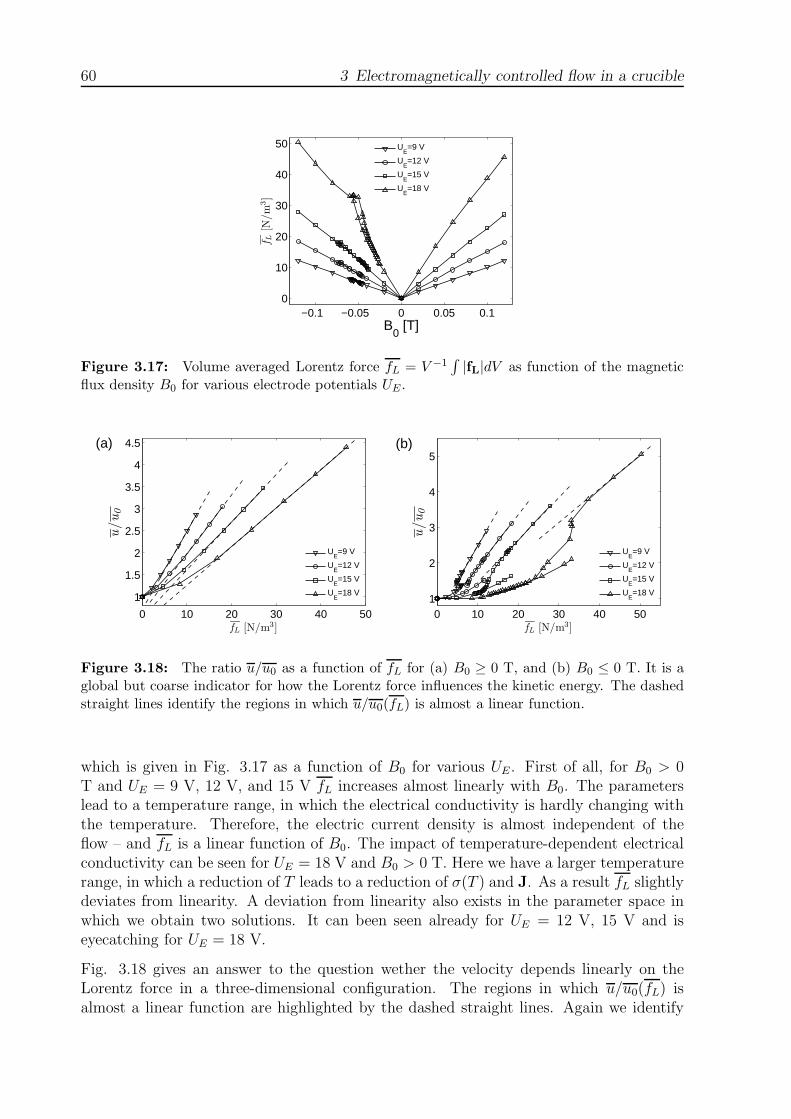
60 3 Electromagnetically controlled flow in a crucible
−0.1 −0.05 0 0.05 0.10
10
20
30
40
50
B0 [T]
f L[N
/m
3]
UE=9 V
UE=12 V
UE=15 V
UE=18 V
Figure 3.17: Volume averaged Lorentz force fL = V −1∫|fL|dV as function of the magnetic
flux density B0 for various electrode potentials UE .
0 10 20 30 40 50
1
1.5
2
2.5
3
3.5
4
4.5
fL [N/m3]
u/u0
UE=9 V
UE=12 V
UE=15 V
UE=18 V
(a)
0 10 20 30 40 501
2
3
4
5
fL [N/m3]
u/u0
UE=9 V
UE=12 V
UE=15 V
UE=18 V
(b)
Figure 3.18: The ratio u/u0 as a function of fL for (a) B0 ≥ 0 T, and (b) B0 ≤ 0 T. It is aglobal but coarse indicator for how the Lorentz force influences the kinetic energy. The dashedstraight lines identify the regions in which u/u0(fL) is almost a linear function.
which is given in Fig. 3.17 as a function of B0 for various UE . First of all, for B0 > 0T and UE = 9 V, 12 V, and 15 V fL increases almost linearly with B0. The parameterslead to a temperature range, in which the electrical conductivity is hardly changing withthe temperature. Therefore, the electric current density is almost independent of theflow – and fL is a linear function of B0. The impact of temperature-dependent electricalconductivity can be seen for UE = 18 V and B0 > 0 T. Here we have a larger temperaturerange, in which a reduction of T leads to a reduction of σ(T ) and J. As a result fL slightlydeviates from linearity. A deviation from linearity also exists in the parameter space inwhich we obtain two solutions. It can been seen already for UE = 12 V, 15 V and iseyecatching for UE = 18 V.
Fig. 3.18 gives an answer to the question wether the velocity depends linearly on theLorentz force in a three-dimensional configuration. The regions in which u/u0(fL) isalmost a linear function are highlighted by the dashed straight lines. Again we identify

3.2 One-dimensional analytical model 61
two regions of linearity: for B0 > 0 T shown in Fig. 3.18(a) and for solutions of the lowerstable branch after the transition from the upper branch with B0 < 0 T shown in Fig.3.18(b).
3.2 One-dimensional analytical model
The numerical studies presented in Sec. 3.1 reveal the influence of the Lorentz force onthe flow structures in glass melt. However, such three-dimensional computations requirelong simulation times. Therefore, they are restricted to a limited number of parameters.In Sec. 3.1 we have varied electric potential between the electrodes UE and the magneticflux density B0 to study the influence of the imposed Lorentz force. We performed thecalculations for one specific glass melt and failed to reveal the difference between therole of the temperature-dependent viscosity and the temperature-dependent electricalconductivity.
One possibility to perform extensive parameter studies and to obtain a deeper under-standing of the basic physics is to develop simplified models which can be studied at lowcomputational cost. The formulation of such a model is the goal of the present section.The large convection rolls which arise in the melting furnace suggest to formulate suchmodels on the basis of the assumption that the fluid is confined to an annular loop whichcontains heating, cooling, and forcing zones. Such assumption enables us to study anone-dimensional form of the fluid flow and to obtain a better understanding of the flowbehavior in a convection roll under the influence of an imposed Lorentz force.
More specifically, our present work is inspired by previous studies on natural circulationloops which consist of at least one heat source and one higher elevated heat sink connectedby pipes. The convection in such loops is driven by buoyancy only. These systems havevarious important applications in energy conservation systems for example solar heatersand cooling systems of nuclear reactors and have been the subject of a large number oftheoretical and experimental studies. Reviews of the wide applications are given by Zvirin[88] and Greif [28]. This field of research was pioneered by Keller [41] and Welander [84]who used natural circulation loops to model geothermal and geophysical processes. TheLorenz-like chaotic alternations of flow directions were also experimentally observed andtheoretically analyzed for example by Creveling et al. [11] and Ehrhard & Muller [16].Beside the most common analytical approach to average the governing equations overthe pipe cross section, Desrayaud et al. [15] performed two-dimensional time-dependentanalysis showing the influence of radial components on the flow characteristic. In a fewworks the fluid of the loop was considered to be electrically conducting. In the presence ofa transverse magnetic field eddy currents and a Lorentz force can be induced and can leadto a damping of the motion. Poddubnaya & Shaidurov [61] studied two hydrodynamicallyconnected vertical pipes heated from below and showed that the onset of convection isa function of the magnetic flux density. Ghaddar analyzed in [21] and [22] the influenceof the magnetic field density on the flow characteristic for similar geometries over a widerange of parameters.
To our knowledge, no analytical studies about the influence of temperature-dependent
62 3 Electromagnetically controlled flow in a crucible
material properties on the flow characteristic of a loop exist in the literature. We al-ready showed in Chapter 2 that the temperature-dependent viscosity modifies the flowsignificantly and can lead to non-linear flow characteristics, instabilities, and multi-valuedsolutions even in simple geometries like pipes. Furthermore, experimental and numericalinvestigations of Rayleigh-Benard convection cells with large viscosity variations exist inthe literature which have been motivated by the Earth’s mantle convection. Already thepioneering works of Torrance & Turcotte [75] and Booker [4] showed the modification ofheat transfer and flow structures due to the temperature-dependent viscosity. For ex-tremely large viscosity variations a stagnant lid developed in the uppermost coldest part.The transition regimes were studied numerically by Ogawa et al. [56] for a 3d configura-tion and have been extended for a wide range of Rayleigh numbers and viscosity contrastup to 1014 for a 2d square cell by Moresi & Solomatov [53]. This overview shows thatalready the investigation of the flow of a fluid with temperature-dependent viscosity in aloop – even without imposed Lorentz force – represents a useful generalization of previousworks.
The present work is a direct continuation of our previous paper [25] which dealt with ananalytical model for a circular loop including a Lorentz force as an additional parameter.This model, like the present one, was motivated by the convection of glass melt in acrucible under the influence of the imposed Lorentz force. The Lorentz force in [25],henceforth referred to as GT5, was generated by an electric current injected directly intothe melt and a perpendicularly acting magnetic field density, whereby both fields wereassumed to be independent of the flow in the loop. The fluid in the loop was consideredto be driven by strongly localized heating and cooling sections. For a wide range ofconditions instabilities were found which led to multiple-valued solutions. Furthermore,this model, in spite of its simplicity, revealed the significant influence of the Lorentz forceon the flow. However, this model did not include some key attributes of convection rollsin glass melts, namely (i) the strong dependence of viscosity and electrical conductivityon the temperature which, in practice, can lead to variations by more than one order ofmagnitude; (ii) the non-circular shape of the convection rolls (cf. the experiments [36] andnumerical simulations [27], Sec. 3.1); (iii) the absence of isothermal regions in convectionrolls.
We now focus on the mentioned characteristics for convection rolls of glass melt (i)–(iii) and present a new model for the highly viscous fluid in a closed loop. Besides theimposed Lorentz force we will study the influence of the variation of electrical conductivityand viscosity on the flow. We will show how the setup of the loop – ranging from twohydrodynamically connected vertical branches to almost circular loops – can modify theflow as well. We will discuss separably the role of Lorentz force, temperature-dependentelectrical conductivity and temperature-dependent viscosity.
3.2.1 Formulation of the problem
We consider a tube of circular cross section with the uniform radius R and the lengthL ≫ R bent to a closed loop with two vertical branches of the length l. The two branchesare connected by two circular arcs with the arc radius r as shown in Fig. 3.19(a). We
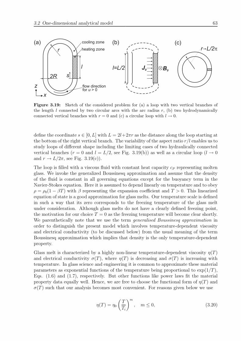
3.2 One-dimensional analytical model 63
s
l
r
cooling zone
heating zone
flow directionfor > 0u
2R
J0 B0
x
z
(a) (b) (c)
l=L/2
r L/2p
Figure 3.19: Sketch of the considered problem for (a) a loop with two vertical branches ofthe length l connected by two circular arcs with the arc radius r, (b) two hydrodynamicallyconnected vertical branches with r = 0 and (c) a circular loop with l → 0.
define the coordinate s ∈ [0, L] with L = 2l+2πr as the distance along the loop starting atthe bottom of the right vertical branch. The variability of the aspect ratio r/l enables us tostudy loops of different shape including the limiting cases of two hydraulically connectedvertical branches (r = 0 and l = L/2, see Fig. 3.19(b)) as well as a circular loop (l → 0and r → L/2π, see Fig. 3.19(c)).
The loop is filled with a viscous fluid with constant heat capacity cP representing moltenglass. We invoke the generalized Boussinesq approximation and assume that the densityof the fluid is constant in all governing equations except for the buoyancy term in theNavier-Stokes equation. Here it is assumed to depend linearly on temperature and to obeyρ = ρ0(1 − βT ) with β representing the expansion coefficient and T > 0. This linearizedequation of state is a good approximation for glass melts. Our temperature scale is definedin such a way that its zero corresponds to the freezing temperature of the glass meltunder consideration. Although glass melts do not have a clearly defined freezing point,the motivation for our choice T = 0 as the freezing temperature will become clear shortly.We parenthetically note that we use the term generalised Boussinesq approximation inorder to distinguish the present model which involves temperature-dependent viscosityand electrical conductivity (to be discussed below) from the usual meaning of the termBoussinesq approximation which implies that density is the only temperature-dependentproperty.
Glass melt is characterized by a highly non-linear temperature-dependent viscosity η(T )and electrical conductivity σ(T ), where η(T ) is decreasing and σ(T ) is increasing withtemperature. In glass science and engineering it is common to approximate these materialparameters as exponential functions of the temperature being proportional to exp(1/T ),Eqs. (1.6) and (1.7), respectively. But other functions like power laws fit the materialproperty data equally well. Hence, we are free to choose the functional form of η(T ) andσ(T ) such that our analysis becomes most convenient. For reasons given below we use
η(T ) = η0
(T
Ti
)m
, m ≤ 0, (3.20)

64 3 Electromagnetically controlled flow in a crucible
with the viscosity parameters η0 and m depending on the glass type. The normalizationfactor Ti is set to 1 K to assure that η0, which does not have a physical meaning, ismeasured in units of the viscosity. Since η → ∞ for T → 0 it becomes clear that thetemperature T = 0 can be regarded as the freezing temperature of the melt. Hence, theviscosity law, eq. (??), only makes sense for T > 0. We further assume
σ(T ) = σ0
(T
Ti
)n
, n ≥ 0, (3.21)
again with constant parameters σ0 and n specific to the considered glass melt. For m =n = 0 the fluid has a constant viscosity, η = η0, and a constant electrical conductivity,σ = σ0, respectively. The advantage of our power laws is their convenient algebraichandling when integrations are necessary. By contrast, the more common models involvingthe temperature dependence exp(1/T ) do not yield to an analytic integration.
On the right vertical branch of the loop, 0 ≤ s ≤ l, a constant electric current density J0 =J0ex is applied and leads to a volumetric heat production according to J2
0/σ. This part ofthe loop is referred to as the heating zone. In the remaining part of the loop, l ≤ s ≤ L, aconstant heat transfer coefficient h is prescribed at the pipe walls. Therefore this branch isnamed cooling zone. The resulting temperature gradient along s leads to buoyancy drivenconvection in a counterclockwise direction. We further assume that a time-independentexternal magnetic flux density B0 = B0ey, which is acting perpendicular to J0 in the rightvertical branch, leads to a Lorentz force density fL = J0B0ez in the melt. Depending on thedirection of B0, the Lorentz force either reinforces or counteracts the thermal convection.For reasons given in Sec. 3.1.1, we neglect the induced current density and effects ofviscous dissipation.
The aim of this work is to derive a simplified model that predicts the cross-section averagedvelocity u and the cross-section averaged temperature distribution T (s) in the loop. Sincewe assume that our glass melt is incompressible, u does not depend on s. By virtue ofour assumption L ≫ R, the one-dimensional model of the flow and heat transfer to bederived below, is expected to be sufficiently accurate, similar to previous works aboutthermal convection loops e.g. by [84], [16] and pipe flow e.g. presented in Chapter 2.
In general, the steady low-Reynolds number flow at hand is governed by the three-dimensional (3d) Stokes equation including Lorentz force and the 3d energy equation.For L ≫ R however, these equations can be reduced to a mathematical model that con-tains the coordinate s only. Since this approach has been extensively used in the past,we will not present the full derivation of the model here and refer the interested readerto the references [84], [16], [25] and [23]. The tangential component of the stationarycross-section averaged Stokes equation
dp
ds= (fv + fb + fL) · es (3.22)
is the relevant source of information to derive our model. This equation expresses thebalance between the viscous fv, buoyancy fb, and Lorentz fL force densities on the onehand, and the pressure gradient dp/ds on the other hand. es is the unit vector tangentialto the loop. Assuming a Poiseuille velocity profile, the viscous friction force becomes

3.2 One-dimensional analytical model 65
fv = −8uη(T (s))/R2es. The buoyancy force is given by the equation fb = ρ0βgT (s)ez,where g denotes the acceleration of gravity. The Lorentz force acts only within the heatingzone (0 ≤ s ≤ l) and reads fL = J0B0ez.
To eliminate the pressure we integrate Eq.(3.22) from s = 0 to s = L. Making use of theuniqueness of the pressure expressed by p(s + L) = p(s) we obtain
8u
R2
L∫
0
η(T (s))ds = ρ0βg
L∫
0
T (s)ez · esds + J0B0l. (3.23)
Eq.(3.23) expresses the balance between the integrated viscous friction on the left-handside and the driving buoyancy and Lorentz force on the right-hand side. The integratedbuoyancy term has to be evaluated separately for each branch as buoyancy acts along thegravitational field in ez-direction. In detail, the buoyancy term takes the form
L∫
0
T (s)ez · esds =
l∫
0
T (s)ds +
l+πr∫
l
T (s) cos
(s − l
r
)ds
−2l+πr∫
l+πr
T (s)ds −L∫
2l+πr
T (s) cos
(s − (2l + πr)
r
)ds.
To derive an equation for the one-dimensional temperature distribution T (s) the heatingand cooling zones have to be considered separately. In the heating zone there is no heatloss to the environment. Instead, the increase of the heat flux carried by the mean flow isequal to the volumetric heating due to the Joule effect. Neglecting effects of heat diffusion,the steady-state energy equation for the heating zone is thus
ρ0cP udT
ds=
J20
σ(T )for s ∈ [0, l]. (3.24)
In the cooling zone the decrease of the heat flux carried by the mean flow is equal to theheat loss through the side wall. This is expressed by the differential equation
ρ0cPudT
ds= −2h
R(T − T∞) for s ∈ [l, L], (3.25)
where T∞ represents the ambient temperature. In the present work we set T∞ = 0 to keepthe model as simple as possible. With this simplification our model is a good approxi-mation for the behavior of a streamline which passes through the immediate vicinity of a(cold) outer wall of a melting crucible which involves strong cooling. However, the presentanalysis can be generalized to nonzero values of T∞. Such model would be appropriate todescribe the behavior of an internal stream line with weak heat transfer. But nonzero val-ues of T∞ would restrict us to a numerical treatment of the basic equations (3.23)-(3.25)instead of an algebraic solution which is one goal of the present work and reachable withT∞ = 0. As T∞ of the 3d simulation in Sec. 3.1 is equal to 1393.15 K, the temperatureT in the loop model represents an offset temperature. In comparison to the simulation itgives the difference between the temperature of the melt and T∞ = 1393.15 K.

66 3 Electromagnetically controlled flow in a crucible
To match the first order differential Eqs. (3.24) and (3.25) the condition of continuitybetween the cooling and heating zone at s = 0 and s = l has to be fulfilled for T . Oncethese equations have been solved for T (s) we are able to evaluate the integrals in theStokes equation (3.23), which then becomes an algebraic equation to determine u.
We non-dimensionalize the governing Eqs. (3.23)-(3.25) using the loop length L as ameasure for all geometry parameters, i.e.:
s = s′L, r = r′L, l = l′L and R = R′L.
Furthermore we use following scales for the velocity u and temperature T :
u = u′u0, with u0 =8η0L
R2ρ0and T = θT0, with T0 =
(J2
0R2T ni
8η0σ0cP
) 1
1+n
.
After substituting these definitions in Eqs. (3.23)-(3.25) and dropping the primes, weobtain the Stokes equation in the form
u
1∫
0
θm(s)ds = Gr
∫ 1
0
θ(s)ez · esds + M, (3.26)
where
Gr =βgρ2
0R4T0
64η20L
(T0
Ti
)−m
(3.27)
is the modified Grashof number which represents the ratio of the square of the viscousdiffusion timescale to the square of the free-fall velocity timescale. Moreover,
M =J0B0lR
4ρ0
64η20L
2
(T0
Ti
)−m
(3.28)
is the modified interaction parameter which can be regarded as the ratio of the Lorentzforce to the viscose force. Let us stress that Gr and M already include the dependence ofviscosity and electrical conductivity on temperature as these parameters are proportionalto (T0/Ti)
−m. The energy equation for the heating zone becomes simply
udθ
ds= θ−n, (3.29)
and the energy equation for the cooling zone becomes
udθ
ds= −Nθ, (3.30)
where
N =hR
4η0cP
(3.31)
is the wall heat loss parameter of the cooling zone. The integration of the non-dimensionalenergy equations (3.29) and (3.30) gives the solution for the temperature distribution
θ(s) =
[(g exp ε)n+1 +
n + 1
us
] 1
n+1
for s ∈ [0, l], (3.32)
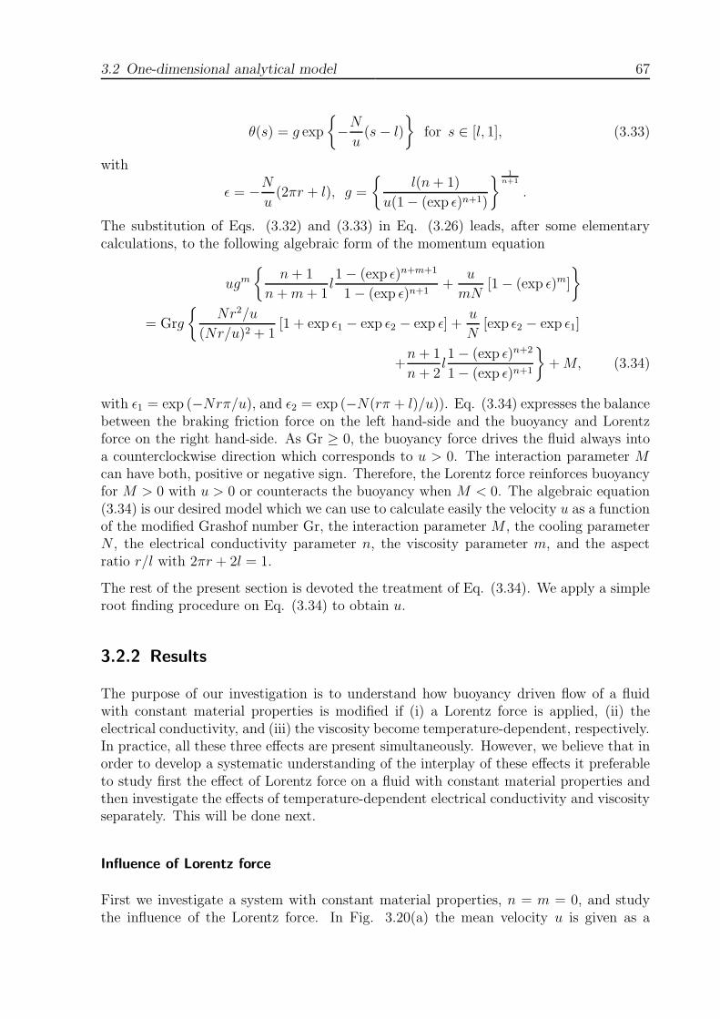
3.2 One-dimensional analytical model 67
θ(s) = g exp
{−N
u(s − l)
}for s ∈ [l, 1], (3.33)
with
ǫ = −N
u(2πr + l), g =
{l(n + 1)
u(1 − (exp ǫ)n+1)
} 1
n+1
.
The substitution of Eqs. (3.32) and (3.33) in Eq. (3.26) leads, after some elementarycalculations, to the following algebraic form of the momentum equation
ugm
{n + 1
n + m + 1l1 − (exp ǫ)n+m+1
1 − (exp ǫ)n+1+
u
mN[1 − (exp ǫ)m]
}
= Grg
{Nr2/u
(Nr/u)2 + 1[1 + exp ǫ1 − exp ǫ2 − exp ǫ] +
u
N[exp ǫ2 − exp ǫ1]
+n + 1
n + 2l1 − (exp ǫ)n+2
1 − (exp ǫ)n+1
}+ M, (3.34)
with ǫ1 = exp (−Nrπ/u), and ǫ2 = exp (−N(rπ + l)/u)). Eq. (3.34) expresses the balancebetween the braking friction force on the left hand-side and the buoyancy and Lorentzforce on the right hand-side. As Gr ≥ 0, the buoyancy force drives the fluid always intoa counterclockwise direction which corresponds to u > 0. The interaction parameter Mcan have both, positive or negative sign. Therefore, the Lorentz force reinforces buoyancyfor M > 0 with u > 0 or counteracts the buoyancy when M < 0. The algebraic equation(3.34) is our desired model which we can use to calculate easily the velocity u as a functionof the modified Grashof number Gr, the interaction parameter M , the cooling parameterN , the electrical conductivity parameter n, the viscosity parameter m, and the aspectratio r/l with 2πr + 2l = 1.
The rest of the present section is devoted the treatment of Eq. (3.34). We apply a simpleroot finding procedure on Eq. (3.34) to obtain u.
3.2.2 Results
The purpose of our investigation is to understand how buoyancy driven flow of a fluidwith constant material properties is modified if (i) a Lorentz force is applied, (ii) theelectrical conductivity, and (iii) the viscosity become temperature-dependent, respectively.In practice, all these three effects are present simultaneously. However, we believe that inorder to develop a systematic understanding of the interplay of these effects it preferableto study first the effect of Lorentz force on a fluid with constant material properties andthen investigate the effects of temperature-dependent electrical conductivity and viscosityseparately. This will be done next.
Influence of Lorentz force
First we investigate a system with constant material properties, n = m = 0, and studythe influence of the Lorentz force. In Fig. 3.20(a) the mean velocity u is given as a
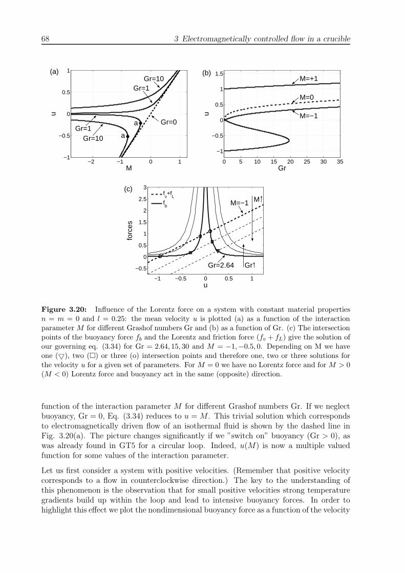
68 3 Electromagnetically controlled flow in a crucible
−2 −1 0 1−1
−0.5
0
0.5
1
Gr=0
Gr=1Gr=10
Gr=1Gr=10
M
u
(a)
a
a
0 5 10 15 20 25 30 35
−1
−0.5
0
0.5
1
1.5
M=−1
M=0
M=+1
Gr
u
(b)
−1 −0.5 0 0.5 1
−0.5
0
0.5
1
1.5
2
2.5
3
M=−1 M
Gr=2.64 Gr
u
forc
es
(c)fv+f
L
fb
Figure 3.20: Influence of the Lorentz force on a system with constant material propertiesn = m = 0 and l = 0.25: the mean velocity u is plotted (a) as a function of the interactionparameter M for different Grashof numbers Gr and (b) as a function of Gr. (c) The intersectionpoints of the buoyancy force fb and the Lorentz and friction force (fv + fL) give the solution ofour governing eq. (3.34) for Gr = 2.64, 15, 30 and M = −1,−0.5, 0. Depending on M we haveone (▽), two (�) or three (o) intersection points and therefore one, two or three solutions forthe velocity u for a given set of parameters. For M = 0 we have no Lorentz force and for M > 0(M < 0) Lorentz force and buoyancy act in the same (opposite) direction.
function of the interaction parameter M for different Grashof numbers Gr. If we neglectbuoyancy, Gr = 0, Eq. (3.34) reduces to u = M . This trivial solution which correspondsto electromagnetically driven flow of an isothermal fluid is shown by the dashed line inFig. 3.20(a). The picture changes significantly if we ”switch on” buoyancy (Gr > 0), aswas already found in GT5 for a circular loop. Indeed, u(M) is now a multiple valuedfunction for some values of the interaction parameter.
Let us first consider a system with positive velocities. (Remember that positive velocitycorresponds to a flow in counterclockwise direction.) The key to the understanding ofthis phenomenon is the observation that for small positive velocities strong temperaturegradients build up within the loop and lead to intensive buoyancy forces. In order tohighlight this effect we plot the nondimensional buoyancy force as a function of the velocity

3.2 One-dimensional analytical model 69
as a solid line in Fig. 3.20(c). This figure shows that fb has a singularity for u = 0. Thesingularity of the buoyancy force for u → 0 occurs for two reasons, namely neglect ofheat conduction along the loop and the linearized density-temperature relationship usedin the Boussinesq approximation. Indeed, since heat cannot be conducted in longitudinaldirection and cannot escape from the insulated heating section, heat builds up withoutbound for u → 0 which leads to θ → 0. If the exact relation ρ(θ) would have been used,ρ would tend to a small but finite value as θ → ∞ leaving the buoyancy force finite.Since we use the linearized relation ρ = ρ0(1 − βθ), instead, ρ → ∞ as θ → ∞ whichgives rise to an infinite buoyancy force. Consequently, the behavior of u(Gr, M) in Figure3.20(a) should be considered as unphysical in the limit M → ∞. If longitudinal heatconduction and non-Boussinesq effects were taken into account, the branches u > 0 andu < 0 for large negative M would be smoothly connected. Nevertheless it is interestingto see that a Lorentz force counteracting the buoyancy force cannot easily stop the flow.The solution u(M) of eq. (3.34) shown in Fig. 3.20(a) can be graphically interpretedas the intersection of the curves fb and fv + fL as functions of u. As indicated in Fig.3.20(c), an intensification of the counteracting Lorentz force (M < 0) leads to a shift of theintersection points along the right branch of fb, but not to a change of the flow direction.
Let us now look at the regime with large and negative velocities which evolves from thedashed straight line in 3.20(a) for M < 0, if we switch on buoyancy. If we start fromstrong negative M and decrease the magnitude of this parameter, the magnitude of themean velocity decreases also until the influence of buoyancy becomes relevant. For u → 0we find hot fluid just below and inside the heating zone and cold fluid in the cooling zone,hence a large buoyancy force builds up acting opposite to the flow direction. To obtaina stable system the driving Lorentz force has to increase very strongly. As a result wefind a turning point in u(M) for u < 0, labeled as a in Fig. 3.20(a). Altogether, forGr > 0 the curve u(M) splits into two branches: One the upper branch with u > 0, thevelocity asymptotically reaches u → 0 for M → −∞ and u = M for u → ∞. The lowerbranch with u < 0 runs from u = M for u → −∞ over the turning point a to u → 0for M → −∞. For M < M(a) three steady solutions for the velocity can be found forone set of parameters. The velocity as a function of Lorentz force was already studied inGT5 for u ≥ 0 and a circular loop. A comparison shows that the results of both modelsagree quantitatively. The physical behavior is reproduced by both models. The resultsfor negative velocities can not be compared as this parameter range has not been studiedin GT5.
The multiple-valued character of u for M < 0 can also be observed if the mean velocityis plotted as a function of the Grashof number Gr as shown in Fig. 3.20(b). The curvefor M = −1 develops two turning points and there exists a range of Gr numbers overwhich three steady states can be found. Between the two turning points we observe acounterintuitive behavior – the magnitude of the clockwise buoyancy force increases aswell. On the upper branch we have u > 0 for all Gr > 0. On the lower branch we haveu < 0 as the clockwise acting Lorentz force is the dominating driving force. Here theabsolute value of the velocity decreases with Gr as buoyancy increases until the turningpoint is reached. If we incidentally increase Gr, buoyancy predominates fb > fL + fv andno equilibrium is reached, see e.g. Fig. 3.20(c). The fluid slows down, buoyancy increasesas the temperature gradient increases and leads to an amplification of the slow down

70 3 Electromagnetically controlled flow in a crucible
process. After the change of the flow direction buoyancy decreases with velocity until thebalance between the forces is reached. This change of flow direction appears in u(Gr)as a jump from the inflexion point of the lower branch with u < 0 to the upper branchwith u > 0. The upper and the lower branches of the curve u(Gr) are stable while themiddle branch is unstable. This can be explained with reference to Fig. 3.20(c) as follows.Consider a state located on the downward sloping branch of the curve u(Gr) for M = 1which corresponds to clockwise motion. Let us assume that an external perturbationleads to slight shift of u in positive direction (i.e. from u to u + du with du > 0) whichcorresponds to a weak ’kick’ in counterclockwise direction. As the curve fb(u) in Fig:3.20(c) shows, the buoyancy force will then change from fb to fb + dfb with fb > 0. Thisimplies that the fluid will experience a force in positive (counterclockwise) direction whichbrakes the clockwise motion further. This closed-loop interaction reinforces the deviationof u from its initial state even further and signifies an unstable branch.
Temperature-dependent electrical conductivity
Now we turn our discussion to a circular loop, 2l ≪ 1, with temperature-dependent elec-trical conductivity, n > 0, and constant viscosity, m = 0. Fig. 3.21(a) shows u as afunction of M for Gr = 10 and various electrical conductivity parameters n. Let us firstnote that the dashed curve with n = 0 in Fig. 3.21(a) and the curve for Gr = 10 in Fig.3.20(a) follow the same characteristics and pertain to similar physical situations. How-ever, the numerical values of both curves are not identical. This quantitative differenceoriginates from the reduction of the length of the heating zone from l = 0.25 (Gr = 10in Fig. 3.20) to l = 0.005 (n = 0 in Fig. 3.21) which leads to a reduction of the heatinput and hence, to a reduction of buoyancy. As a result, the velocity becomes smallerin a buoyancy dominated regime (e.g. M = 0) and the turning point shifts to velocitieswith a smaller magnitude for the present system with l = 0.005.
Furthermore, Fig. 3.21(a) shows that the temperature-dependent electrical conductivityleads to a dramatic change of the flow characteristic u(M). In the case M < 0 are regionswhere there exist three solutions for u. Such a multiple-valued solution can also be foundif we plot u as function of the Grashof number Gr as it is done in Fig. 3.21(b). If theLorentz force acts against buoyancy, M < 0, and M reaches a certain critical value, thereis a range of Grashof numbers over which three steady states can be found for positivevelocities, see the curve with M = −1 in Fig. 3.21(b). The curve develops two turningpoints, which are labeled with a and b in Fig. 3.21(b). We note that between thesetwo points there are solutions for which the velocity decreases as the Grashof numberincreases. Without Lorentz forces, M = 0 (dashed line in Fig. 3.21(b)), u is a monotonicnon-linear function of Gr and u increases with n as buoyancy increases, see Fig. 3.21(a).
An explanation of the triple-valued solution can be given with the help of the acting forcesas functions of u. In Fig. 3.21(c) the sum of the braking friction and Lorentz force fv +fL
(dashed line) and the driving buoyancy fb (solid line) for different Gr numbers are given.For u/|M | > 1 the friction force gives the dominating contribution to the braking forcesfv ≫ fL with fv = u. For u/|M | < 1 we have fL = M as the Lorentz force dominatesfL ≫ fv. Interestingly, however, buoyancy fb(u) turns out to be not a monotonically
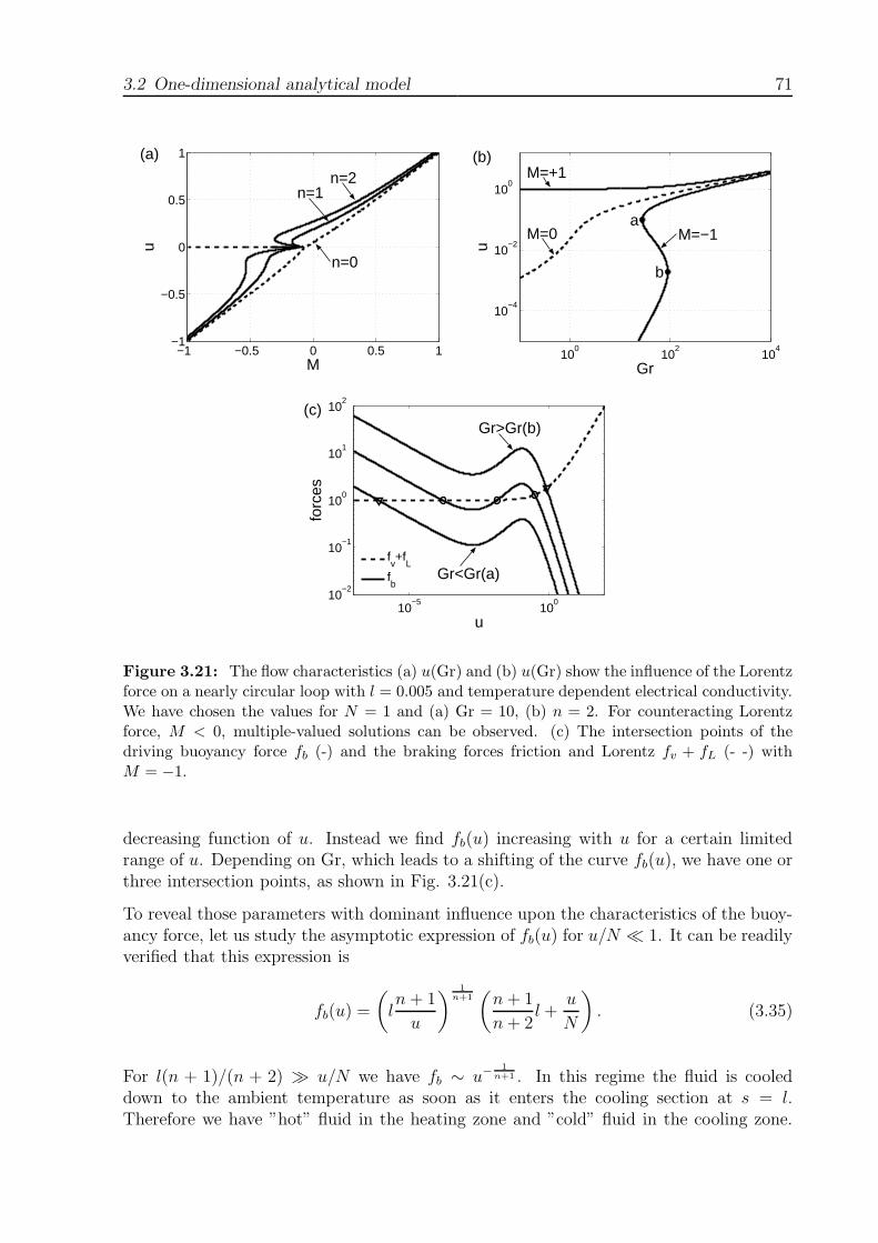
3.2 One-dimensional analytical model 71
−1 −0.5 0 0.5 1−1
−0.5
0
0.5
1
n=0
n=1n=2
M
u(a)
100
102
104
10−4
10−2
100
a
b
M=−1M=0
M=+1
Gr
u
(b)
10−5
100
10−2
10−1
100
101
102
Gr<Gr(a)
Gr>Gr(b)
u
forc
es
(c)
fv+f
L
fb
Figure 3.21: The flow characteristics (a) u(Gr) and (b) u(Gr) show the influence of the Lorentzforce on a nearly circular loop with l = 0.005 and temperature dependent electrical conductivity.We have chosen the values for N = 1 and (a) Gr = 10, (b) n = 2. For counteracting Lorentzforce, M < 0, multiple-valued solutions can be observed. (c) The intersection points of thedriving buoyancy force fb (-) and the braking forces friction and Lorentz fv + fL (- -) withM = −1.
decreasing function of u. Instead we find fb(u) increasing with u for a certain limitedrange of u. Depending on Gr, which leads to a shifting of the curve fb(u), we have one orthree intersection points, as shown in Fig. 3.21(c).
To reveal those parameters with dominant influence upon the characteristics of the buoy-ancy force, let us study the asymptotic expression of fb(u) for u/N ≪ 1. It can be readilyverified that this expression is
fb(u) =
(ln + 1
u
) 1
n+1(
n + 1
n + 2l +
u
N
). (3.35)
For l(n + 1)/(n + 2) ≫ u/N we have fb ∼ u−1
n+1 . In this regime the fluid is cooleddown to the ambient temperature as soon as it enters the cooling section at s = l.Therefore we have ”hot” fluid in the heating zone and ”cold” fluid in the cooling zone.
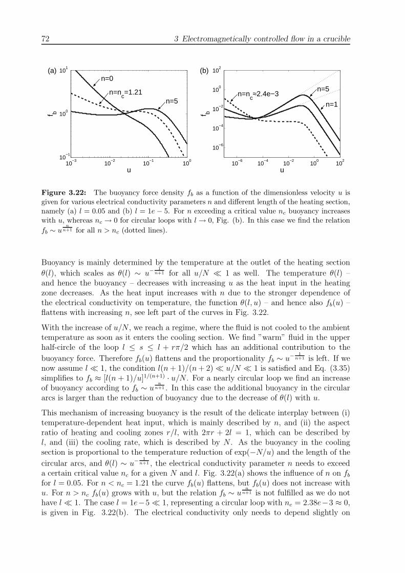
72 3 Electromagnetically controlled flow in a crucible
10−3
10−2
10−1
100
10−1
100
101
n=5
n=0
n=nc=1.21
u
f b
(a)
100
102
10−2
10−4
10−6
100
102
10−2
10−4
10−6
n=nc≈2.4e−3
n=5
n=1
u
f b
(b)
Figure 3.22: The buoyancy force density fb as a function of the dimensionless velocity u isgiven for various electrical conductivity parameters n and different length of the heating section,namely (a) l = 0.05 and (b) l = 1e − 5. For n exceeding a critical value nc buoyancy increaseswith u, whereas nc → 0 for circular loops with l → 0, Fig. (b). In this case we find the relation
fb ∼ un
n+1 for all n > nc (dotted lines).
Buoyancy is mainly determined by the temperature at the outlet of the heating section
θ(l), which scales as θ(l) ∼ u−1
n+1 for all u/N ≪ 1 as well. The temperature θ(l) –and hence the buoyancy – decreases with increasing u as the heat input in the heatingzone decreases. As the heat input increases with n due to the stronger dependence ofthe electrical conductivity on temperature, the function θ(l, u) – and hence also fb(u) –flattens with increasing n, see left part of the curves in Fig. 3.22.
With the increase of u/N , we reach a regime, where the fluid is not cooled to the ambienttemperature as soon as it enters the cooling section. We find ”warm” fluid in the upperhalf-circle of the loop l ≤ s ≤ l + rπ/2 which has an additional contribution to the
buoyancy force. Therefore fb(u) flattens and the proportionality fb ∼ u−1
n+1 is left. If wenow assume l ≪ 1, the condition l(n + 1)/(n + 2) ≪ u/N ≪ 1 is satisfied and Eq. (3.35)simplifies to fb ≈ [l(n + 1)/u]1/(n+1) · u/N . For a nearly circular loop we find an increaseof buoyancy according to fb ∼ u
n
n+1 . In this case the additional buoyancy in the circulararcs is larger than the reduction of buoyancy due to the decrease of θ(l) with u.
This mechanism of increasing buoyancy is the result of the delicate interplay between (i)temperature-dependent heat input, which is mainly described by n, and (ii) the aspectratio of heating and cooling zones r/l, with 2πr + 2l = 1, which can be described byl, and (iii) the cooling rate, which is described by N . As the buoyancy in the coolingsection is proportional to the temperature reduction of exp(−N/u) and the length of the
circular arcs, and θ(l) ∼ u−1
n+1 , the electrical conductivity parameter n needs to exceeda certain critical value nc for a given N and l. Fig. 3.22(a) shows the influence of n on fb
for l = 0.05. For n < nc = 1.21 the curve fb(u) flattens, but fb(u) does not increase withu. For n > nc fb(u) grows with u, but the relation fb ∼ u
n
n+1 is not fulfilled as we do nothave l ≪ 1. The case l = 1e−5 ≪ 1, representing a circular loop with nc = 2.38e−3 ≈ 0,is given in Fig. 3.22(b). The electrical conductivity only needs to depend slightly on
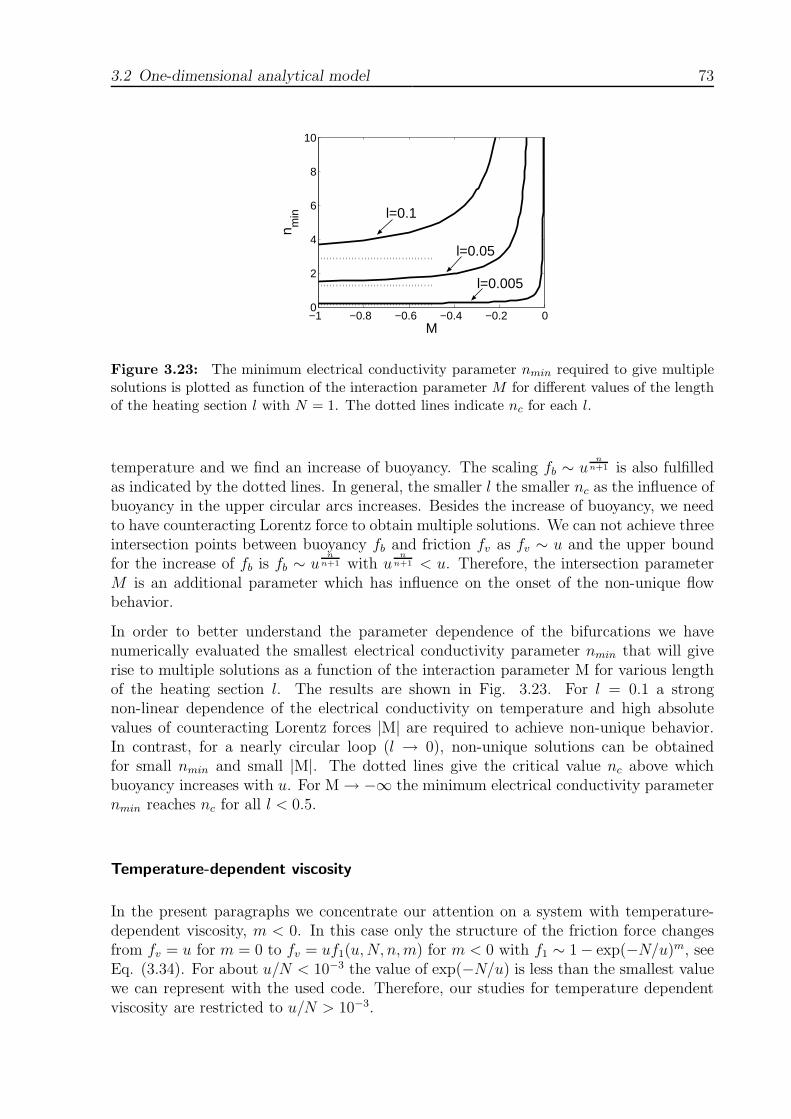
3.2 One-dimensional analytical model 73
−1 −0.8 −0.6 −0.4 −0.2 00
2
4
6
8
10
l=0.1
l=0.05
l=0.005
M
n min
Figure 3.23: The minimum electrical conductivity parameter nmin required to give multiplesolutions is plotted as function of the interaction parameter M for different values of the lengthof the heating section l with N = 1. The dotted lines indicate nc for each l.
temperature and we find an increase of buoyancy. The scaling fb ∼ un
n+1 is also fulfilledas indicated by the dotted lines. In general, the smaller l the smaller nc as the influence ofbuoyancy in the upper circular arcs increases. Besides the increase of buoyancy, we needto have counteracting Lorentz force to obtain multiple solutions. We can not achieve threeintersection points between buoyancy fb and friction fv as fv ∼ u and the upper boundfor the increase of fb is fb ∼ u
n
n+1 with un
n+1 < u. Therefore, the intersection parameterM is an additional parameter which has influence on the onset of the non-unique flowbehavior.
In order to better understand the parameter dependence of the bifurcations we havenumerically evaluated the smallest electrical conductivity parameter nmin that will giverise to multiple solutions as a function of the interaction parameter M for various lengthof the heating section l. The results are shown in Fig. 3.23. For l = 0.1 a strongnon-linear dependence of the electrical conductivity on temperature and high absolutevalues of counteracting Lorentz forces |M| are required to achieve non-unique behavior.In contrast, for a nearly circular loop (l → 0), non-unique solutions can be obtainedfor small nmin and small |M|. The dotted lines give the critical value nc above whichbuoyancy increases with u. For M → −∞ the minimum electrical conductivity parameternmin reaches nc for all l < 0.5.
Temperature-dependent viscosity
In the present paragraphs we concentrate our attention on a system with temperature-dependent viscosity, m < 0. In this case only the structure of the friction force changesfrom fv = u for m = 0 to fv = uf1(u, N, n, m) for m < 0 with f1 ∼ 1 − exp(−N/u)m, seeEq. (3.34). For about u/N < 10−3 the value of exp(−N/u) is less than the smallest valuewe can represent with the used code. Therefore, our studies for temperature dependentviscosity are restricted to u/N > 10−3.

74 3 Electromagnetically controlled flow in a crucible
−20 −10 0 10 20−1
−0.5
0
0.5
1
m=−0.2
m=−2m=0
M
u
(a)
100
102
104
106
10−2
10−3
10−2
10−1
100
101
m=−0.02
m=−0.2
m=−2
Gr
u
(b)
10−2
100
102
10−2
100
102
m=−0.02
m=−0.2m=−2
u
forc
es
(c)
fv
fb
Figure 3.24: The dimensionless velocity u as a function of (a) the interaction parameter Mwith Gr = 10 and (b) the Grashof number Gr for a system without Lorentz force M = 0 fordifferent values of the viscosity parameter m with n = 0, N = 1, l = 0.25. (c) The correspondingforce distribution for (b) of the the driving buoyancy fb (-) and braking friction force fv (- -)for Gr = 0.23 as function of u for different viscosity parameters m. As the friction force has aparabolic-like profile we obtain two (o), one (▽) or no intersection points between fb and fv.
If the regime of constant viscosity with m = 0 is left, u(M) changes qualitatively as it isshown in Fig. 3.24(a). For moderate m (e.g. m = −0.2) there is virtually no differencebetween the temperature-dependent and the constant viscosity on the lower branch withu < 0. By contrast, on the upper stable branch with u > 0 we find a turning point suchthat u → 0 for M → +∞ and we have four values for u for one M . If the dependence ofviscosity on temperature is strong (e.g. m = −2), the graph resembles a hyperbola. Fora given Gr we need a certain |M | to obtain a solution.
To understand this observation, let us study the mean velocity u as function of Gr fordifferent viscosity parameters m and no Lorentz force (M = 0). Fig. 3.24(b) shows thatthe temperature dependent viscosity separates the parameter space into three regimes:(i) the stagnant regime, (ii) the single-valued regime and (iii) the double-valued regime.The single-valued regime – characterized by a single velocity as solution for a given set ofparameters – can only be obtained for a certain Grashof numbers, which we also denote as

3.2 One-dimensional analytical model 75
0 200 400 600 800−3.5
−3
−2.5
−2
−1.5
−1
−0.5
0
Grc
mc
two−valued regime
stagnant regime
Figure 3.25: The phase diagram gives the region of parameters in which the fluid is immo-bilized – stagnant regime – and in which two solutions do coexist – two-valued regime – forM = n = 0, N = 1 and l = 0.25. Both regimes are separated by the one valued regime which ischaracterized by critical Grashof number Grc (solid line).
the critical Grashof number Grc. This point in the parameter space forms the overturningpoint of u(Gr). If the Grashof number exceeds this critical value, i.e. Gr > Grc, we reachthe double-valued regime and obtain two velocities for one given Gr. Here, for largevelocities, u is a increasing function of Gr as it is known from thermal convection. Forsmall velocities, however, u decreases with increasing Gr. For Gr < Grc we did not founda solution at all. The phase diagram in Fig. 3.25 summarizes the region of parametersfor all three regimes (i)-(iii).
The reason for the stagnant regime is the shape of the friction force given in Fig. 3.24(c).For large velocities we have small temperature differences and therefore small viscositydifferences within the loop. The friction force is proportional to u. In the case of smallvelocities the temperature in the cooling zone tends to θ → 0 and hence, the viscosityleads to η → ∞. Thus, the friction force fv strongly increases with decreasing u. As aresult fv(u) has a parabola-like shape with a minimum friction force. As the buoyancycurve is monotonically decreasing with u, we obtain two, one or none intersection pointsand therefore two, one or no solution as shown in Fig. 3.24(c).
From the two intersection points only the right one is stable and hence, only the upperbranch of the two-valued solution is stable. Any u that is slightly above the lower branchwill drive the system to the upper stable branch while any u slightly below the lowerbranch will initiate freezing of the system. Such freezing is not necessarily a contraction.It has been observed for forced convection of glass melt in a pipe in industrial processingand was confirmed theoretically [48], [24]. In practice freezing typically occurs if the meltis cooled by room temperature (for which η → ∞) and if the velocity is below a criticalvalue. In a convection cell, a stagnant layer develops and the motion shifts away fromthe cold walls. In glass processing such a behavior is used in cold induction crucibles tominimize corrosion at the crucible wall. As the fluid motion in the model is restricted to adefined path, the loop can not reflect the structural modification of convection cells whichis a limit of the thermosyphon approach in general. However, a second stable branch of

76 3 Electromagnetically controlled flow in a crucible
u(Gr), Fig. 3.24(a), exists theoretically. We would be able to calculate this branch, ifη would have a finite value for θ∞. This could be realized for example with the presentviscosity law, equation (??), and θ∞ > 0. In this case the friction law fv(u) would obtaina third branch for u → 0 for which fv is a linear function of u and one would obtain 1 to3 intersection points.
3.3 Comparison between numerical, analytical, and
experimental results
In the previous sections 3.1 and 3.2 we have presented parameter studies for electromag-netically driven convection of molten glass in a crucible by three-dimensional numericalsimulations and by one-dimensional modeling. Now we compare the results of these twoapproaches with each other. Furthermore, we link the results with the experimental dataobtained by Krieger, which are published in [42]. The comparison between the experimentand the numerical simulation is straight forward as the geometry and the boundary con-ditions of the numerical model meet the experimental setup. But the comparison with theresults of the analytical model requires some adjustments of the model parameters and thetransformation of the material property laws from the common exponential formulation,Eqs. (1.6), (1.7), into the power law formulation, Eqs. (3.20) and (3.21). Therefore, wefirst describe these adjustments and then present some results of glass melt flow in theone-dimensional loop given in SI units. Afterwards, we compare all approaches with eachother.
3.3.1 Adjustment of model parameters and material property laws
Even though the 1d analytical loop model is inspired by the 3d crucible configurationand captures the main physics of the system, the reduction from the 3d setup to the 1dsystem leads to some differences between both approaches and requires the adjustmentof some parameters. These parameters are the geometry parameters of the loop whichrepresents the vortex flow in the crucible. We also have to adjust the current densityJ0, the magnetic flux density B0, and the heat transfer coefficient h. In the loop modelJ0 and B0 are applied in the heating zone only, whereas the current density J and B0
capture the total volume of the melt of the 3d configuration. Additionally, J0 is constantin the 1d model whereas J varies within the melt of the 3d configuration. Furthermore,the heat transfer to the surrounding is realized by convective cooling only. But in the 3dsetup we have radiative heat transfer at the free surface beside convective transfer at thecrucible wall. Therefore, the heat transfer coefficient has to be modified to meet roughlythe overall heat loss of the 3d configuration. For a detailed comparison of the geometryand model parameters we refer to Figs. 3.1, 3.2, 3.19 and Secs. 3.1.1, 3.2.1, respectively.Overall, many possibilities exist to adjust the mentioned model parameters of the loop.In the following we sketch the possibility which we have used for our calculations. We donot claim that it is the one and only parameter adjustment.

3.3 Comparison between numerical, analytical, and experimental results 77
We have performed the calculations with the following loop geometry parameters: lengthof the heating zone l = 0.04 m, arc radius r = 0.02 m, and inner diameter of the piped = 0.02 m.
For the estimation of J0 we start with the requirement that the total heat input Q = J2V/σis equal for all approaches. We then assume that σ is the same in all approaches. In ad-dition, the volume-averaged current density J =
∫JdV/V is known. Consequently, we
can approximate J0 by the following relation:
J0 =
√V
V0· J = 2.77J, (3.36)
with V being the volume of the melt in the 3d crucible, and V0 being the volume of theheating zone. J can be calculated easily in the numerical simulation. From the experimentwe just know the magnitudes of the current I and UE which are applied at the electrodes.Here we propose to calculate J on the basis of the total heat input Q = IUE according toJ =
√Qσ/V . Due to its dependence on the temperature the electrical conductivity σ is
the critical parameter of this relation. Only the knowledge of the operating temperaturerange can lead to a coarse estimation of σ.
Furthermore, we propose a volume-weighting of the magnetic flux densities for the ad-justment of B0. To distinguish between the magnetic flux densities of the 1d and the 3dconfiguration, henceforth we denote B0,1d as the density of the 1d model and B0,3d as thedensity of the 3d configuration. Hence,
B0,1d =V
V0· B0,3d = 7.68B0,3d. (3.37)
To adjust the heat transfer coefficient h we first determine the heat radiation qrad accordingto qrad = σǫ(T 4 − T 4
∞) with T∞ = 1393.15 K and ∆T = T − T∞ = 50 K. Then we
estimate the heat transfer coefficient hrad, which leads to the same heat loss qrad = hrad∆T .Furthermore, we assume that radiation takes place at a half of the upper circular arc witha length of srad = πr/2. At the remaining parts of the cooling zone with a lengthof sconv = 3πr/2 + l we have pure convection which is specified by the heat transfercoefficient hconv. Now the overall heat transfer coefficient h of the cooling zone of the loopis length-weighted and calculates from
h ≈ hconvsconv + hradsrad
sconv + srad
≈ 77W
m2K. (3.38)
For the adjustment of the material properties let us remember that we have set theambient temperature T∞ to zero in the loop model and to 1393.15 K in the simulationand experiment. Hence, the loop model gives an offset temperature which is the differencebetween the temperature of the melt and 1393.15 K. If this offset temperature tends tozero, the power law formulation of the material properties which we used in the analyticalmodel tends to η → ∞ and σ → 0 according to Eqs. (3.20) and (3.21). However, inreality and with the exponential formula, Eqs. (1.6) and (1.7), both properties have afinite non-zero magnitude as soon as the melt temperature tends to 1393.15 K. Hence,
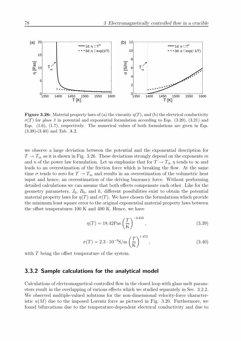
78 3 Electromagnetically controlled flow in a crucible
1350 1400 1450 1500 1550 16000
5
10
15
20
T∞
T [K]
η [P
as]
1d: η ∼ Tm
3d: η ∼ exp(1/T)
(a)
1350 1400 1450 1500 1550 16000
2
4
6
8
10
12
T∞
T [K]
σ [S
/m]
1d: σ ∼ Tn
3d: σ ∼ exp(−1/T)
(b)
Figure 3.26: Material property laws of (a) the viscosity η(T ), and (b) the electrical conductivityσ(T ) for glass 3 in potential and exponential formulation according to Eqs. (3.20), (3.21) andEqs. (1.6), (1.7), respectively. The numerical values of both formulations are given in Eqs.(3.39)-(3.40) and Tab. A.2.
we observe a large deviation between the potential and the exponential description forT → T∞ as it is shown in Fig. 3.26. These deviations strongly depend on the exponents mand n of the power law formulation. Let us emphasize that for T → T∞ η tends to ∞ andleads to an overestimation of the friction force which is breaking the flow. At the sametime σ tends to zero for T → T∞ and results in an overestimation of the volumetric heatinput and hence, an overestimation of the driving buoyancy force. Without performingdetailed calculations we can assume that both effects compensate each other. Like for thegeometry parameters, J0, B0, and h, different possibilities exist to obtain the potentialmaterial property laws for η(T ) and σ(T ). We have chosen the formulations which providethe minimum least square error to the original exponential material property laws betweenthe offset temperatures 100 K and 400 K. Hence, we have
η(T ) = 18.42Pas
(T
K
)−0.635
, (3.39)
σ(T ) = 2.3 · 10−3S/m
(T
K
)1.472
, (3.40)
with T being the offset temperature of the system.
3.3.2 Sample calculations for the analytical model
Calculations of electromagnetical controlled flow in the closed loop with glass melt param-eters result in the overlapping of various effects which we studied separately in Sec. 3.2.2.We observed multiple-valued solutions for the non-dimensional velocity-force character-istic u(M) due to the imposed Lorentz force as pictured in Fig. 3.20. Furthermore, wefound bifurcations due to the temperature-dependent electrical conductivity and due to
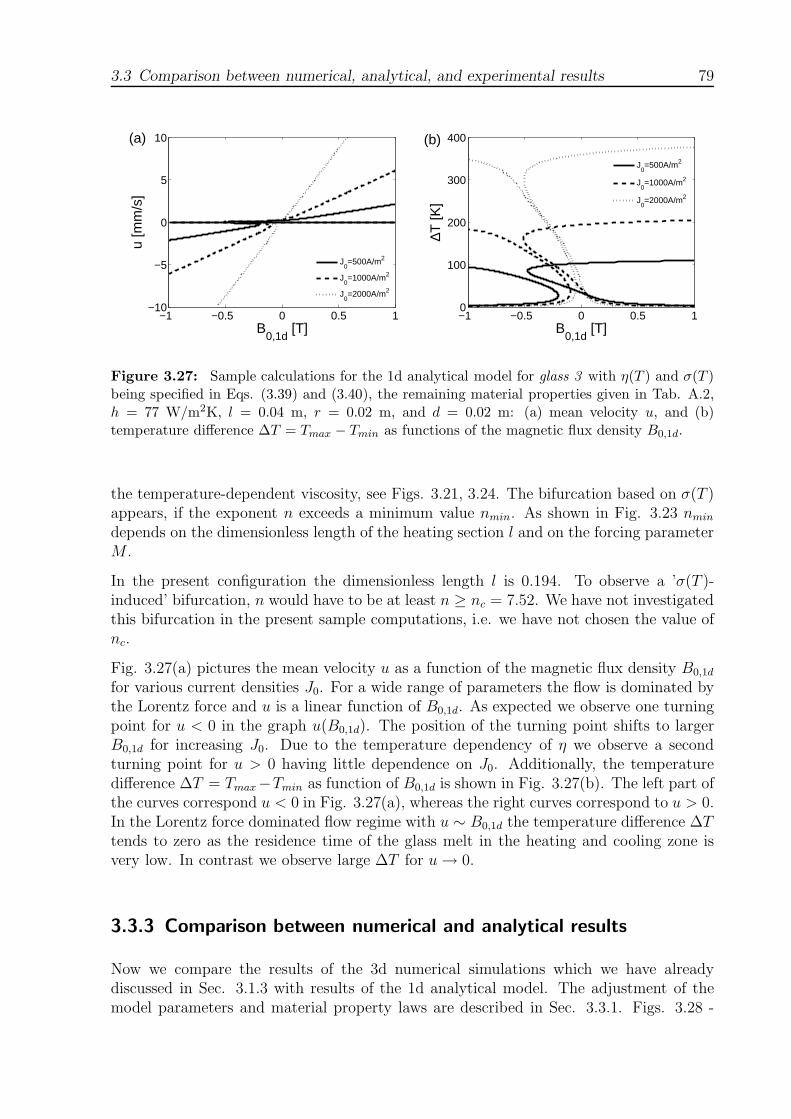
3.3 Comparison between numerical, analytical, and experimental results 79
−1 −0.5 0 0.5 1−10
−5
0
5
10
B0,1d
[T]
u [m
m/s
]
J0=500A/m2
J0=1000A/m2
J0=2000A/m2
(a)
−1 −0.5 0 0.5 10
100
200
300
400
B0,1d
[T]
∆T [K
]
J0=500A/m2
J0=1000A/m2
J0=2000A/m2
(b)
Figure 3.27: Sample calculations for the 1d analytical model for glass 3 with η(T ) and σ(T )being specified in Eqs. (3.39) and (3.40), the remaining material properties given in Tab. A.2,h = 77 W/m2K, l = 0.04 m, r = 0.02 m, and d = 0.02 m: (a) mean velocity u, and (b)temperature difference ∆T = Tmax − Tmin as functions of the magnetic flux density B0,1d.
the temperature-dependent viscosity, see Figs. 3.21, 3.24. The bifurcation based on σ(T )appears, if the exponent n exceeds a minimum value nmin. As shown in Fig. 3.23 nmin
depends on the dimensionless length of the heating section l and on the forcing parameterM .
In the present configuration the dimensionless length l is 0.194. To observe a ’σ(T )-induced’ bifurcation, n would have to be at least n ≥ nc = 7.52. We have not investigatedthis bifurcation in the present sample computations, i.e. we have not chosen the value ofnc.
Fig. 3.27(a) pictures the mean velocity u as a function of the magnetic flux density B0,1d
for various current densities J0. For a wide range of parameters the flow is dominated bythe Lorentz force and u is a linear function of B0,1d. As expected we observe one turningpoint for u < 0 in the graph u(B0,1d). The position of the turning point shifts to largerB0,1d for increasing J0. Due to the temperature dependency of η we observe a secondturning point for u > 0 having little dependence on J0. Additionally, the temperaturedifference ∆T = Tmax−Tmin as function of B0,1d is shown in Fig. 3.27(b). The left part ofthe curves correspond u < 0 in Fig. 3.27(a), whereas the right curves correspond to u > 0.In the Lorentz force dominated flow regime with u ∼ B0,1d the temperature difference ∆Ttends to zero as the residence time of the glass melt in the heating and cooling zone isvery low. In contrast we observe large ∆T for u → 0.
3.3.3 Comparison between numerical and analytical results
Now we compare the results of the 3d numerical simulations which we have alreadydiscussed in Sec. 3.1.3 with results of the 1d analytical model. The adjustment of themodel parameters and material property laws are described in Sec. 3.3.1. Figs. 3.28 -
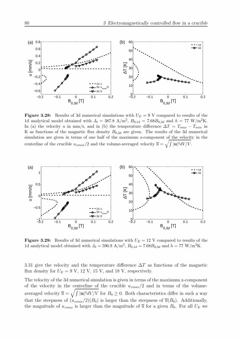
80 3 Electromagnetically controlled flow in a crucible
−0.2 −0.1 0 0.1 0.2
−0.6
−0.4
−0.2
0
0.2
0.4
0.6
0.8
B0,3d
[T]
u [m
m/s
]
1d: u3d: u
zmax/2
3d: u
(a)
−0.2 −0.1 0 0.1 0.20
10
20
30
40
50
60
B0,3d
[T]
∆T [K
]
1d3d
(b)
Figure 3.28: Results of 3d numerical simulations with UE = 9 V compared to results of the1d analytical model obtained with J0 = 387.8 A/m2, B0,1d = 7.68B0,3d and h = 77 W/m2K.In (a) the velocity u in mm/s, and in (b) the temperature difference ∆T = Tmax − Tmin inK as functions of the magnetic flux density B0,3d are given. The results of the 3d numericalsimulation are given in terms of one half of the maximum z-component of the velocity in the
centerline of the crucible uzmax/2 and the volume-averaged velocity u =√∫
|u|2dV/V .
−0.2 −0.1 0 0.1 0.2−1
−0.5
0
0.5
1
B0,3d
[T]
u [m
m/s
]
1d: u3d: u
zmax/2
3d: u
(a)
−0.2 −0.1 0 0.1 0.20
10
20
30
40
50
60
B0,3d
[T]
∆T [K
]
1d3d
(b)
Figure 3.29: Results of 3d numerical simulations with UE = 12 V compared to results of the1d analytical model obtained with J0 = 596.9 A/m2, B0,1d = 7.68B0,3d and h = 77 W/m2K.
3.31 give the velocity and the temperature difference ∆T as functions of the magneticflux density for UE = 9 V, 12 V, 15 V, and 18 V, respectively.
The velocity of the 3d numerical simulation is given in terms of the maximum z-componentof the velocity in the centerline of the crucible uzmax/2 and in terms of the volume-
averaged velocity u =√∫
|u|2dV/V for B0 ≥ 0. Both characteristics differ in such a way
that the steepness of (uzmax/2)(B0) is larger than the steepness of u(B0). Additionally,the magnitude of uzmax is larger than the magnitude of u for a given B0. For all UE we
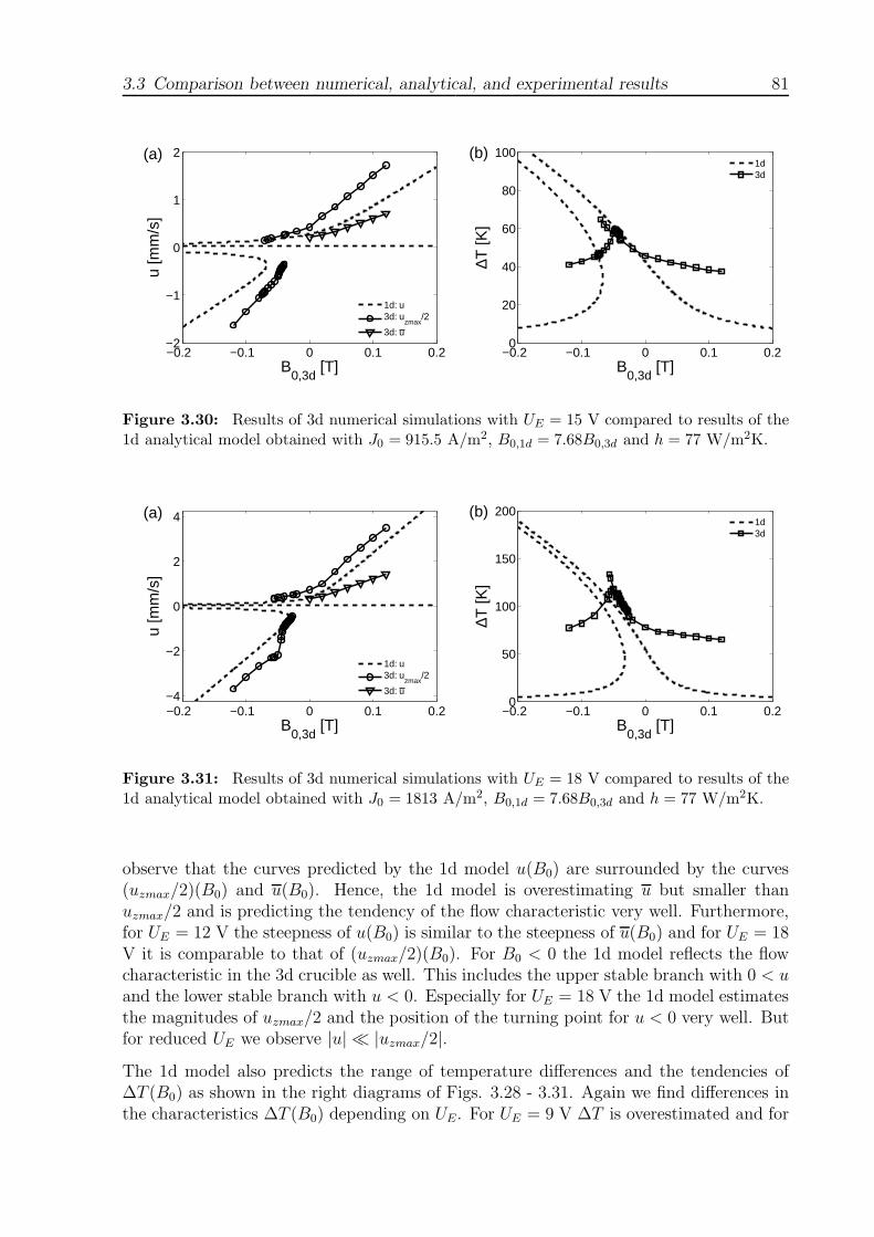
3.3 Comparison between numerical, analytical, and experimental results 81
−0.2 −0.1 0 0.1 0.2−2
−1
0
1
2
B0,3d
[T]
u [m
m/s
]
1d: u3d: u
zmax/2
3d: u
(a)
−0.2 −0.1 0 0.1 0.20
20
40
60
80
100
B0,3d
[T]
∆T [K
]
1d3d
(b)
Figure 3.30: Results of 3d numerical simulations with UE = 15 V compared to results of the1d analytical model obtained with J0 = 915.5 A/m2, B0,1d = 7.68B0,3d and h = 77 W/m2K.
−0.2 −0.1 0 0.1 0.2−4
−2
0
2
4
B0,3d
[T]
u [m
m/s
]
1d: u3d: u
zmax/2
3d: u
(a)
−0.2 −0.1 0 0.1 0.20
50
100
150
200
B0,3d
[T]
∆T [K
]
1d3d
(b)
Figure 3.31: Results of 3d numerical simulations with UE = 18 V compared to results of the1d analytical model obtained with J0 = 1813 A/m2, B0,1d = 7.68B0,3d and h = 77 W/m2K.
observe that the curves predicted by the 1d model u(B0) are surrounded by the curves(uzmax/2)(B0) and u(B0). Hence, the 1d model is overestimating u but smaller thanuzmax/2 and is predicting the tendency of the flow characteristic very well. Furthermore,for UE = 12 V the steepness of u(B0) is similar to the steepness of u(B0) and for UE = 18V it is comparable to that of (uzmax/2)(B0). For B0 < 0 the 1d model reflects the flowcharacteristic in the 3d crucible as well. This includes the upper stable branch with 0 < uand the lower stable branch with u < 0. Especially for UE = 18 V the 1d model estimatesthe magnitudes of uzmax/2 and the position of the turning point for u < 0 very well. Butfor reduced UE we observe |u| ≪ |uzmax/2|.The 1d model also predicts the range of temperature differences and the tendencies of∆T (B0) as shown in the right diagrams of Figs. 3.28 - 3.31. Again we find differences inthe characteristics ∆T (B0) depending on UE. For UE = 9 V ∆T is overestimated and for
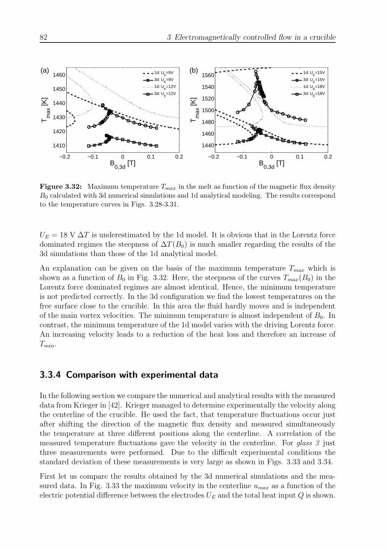
82 3 Electromagnetically controlled flow in a crucible
−0.2 −0.1 0 0.1 0.2
1410
1420
1430
1440
1450
1460
B0,3d
[T]
Tm
ax [K
]
1d: UE=9V
3d: UE=9V
1d: UE=12V
3d: UE=12V
(a)
−0.2 −0.1 0 0.1 0.2
1440
1460
1480
1500
1520
1540
1560
B0,3d
[T]
Tm
ax [K
]
1d: UE=15V
3d: UE=15V
1d: UE=18V
3d: UE=18V
(b)
Figure 3.32: Maximum temperature Tmax in the melt as function of the magnetic flux densityB0 calculated with 3d numerical simulations and 1d analytical modeling. The results correspondto the temperature curves in Figs. 3.28-3.31.
UE = 18 V ∆T is underestimated by the 1d model. It is obvious that in the Lorentz forcedominated regimes the steepness of ∆T (B0) is much smaller regarding the results of the3d simulations than those of the 1d analytical model.
An explanation can be given on the basis of the maximum temperature Tmax which isshown as a function of B0 in Fig. 3.32. Here, the steepness of the curves Tmax(B0) in theLorentz force dominated regimes are almost identical. Hence, the minimum temperatureis not predicted correctly. In the 3d configuration we find the lowest temperatures on thefree surface close to the crucible. In this area the fluid hardly moves and is independentof the main vortex velocities. The minimum temperature is almost independent of B0. Incontrast, the minimum temperature of the 1d model varies with the driving Lorentz force.An increasing velocity leads to a reduction of the heat loss and therefore an increase ofTmin.
3.3.4 Comparison with experimental data
In the following section we compare the numerical and analytical results with the measureddata from Krieger in [42]. Krieger managed to determine experimentally the velocity alongthe centerline of the crucible. He used the fact, that temperature fluctuations occur justafter shifting the direction of the magnetic flux density and measured simultaneouslythe temperature at three different positions along the centerline. A correlation of themeasured temperature fluctuations gave the velocity in the centerline. For glass 3 justthree measurements were performed. Due to the difficult experimental conditions thestandard deviation of these measurements is very large as shown in Figs. 3.33 and 3.34.
First let us compare the results obtained by the 3d numerical simulations and the mea-sured data. In Fig. 3.33 the maximum velocity in the centerline umax as a function of theelectric potential difference between the electrodes UE and the total heat input Q is shown.
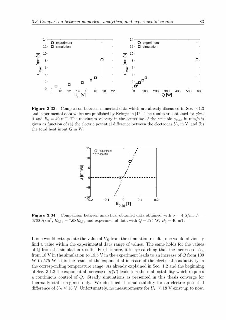
3.3 Comparison between numerical, analytical, and experimental results 83
8 10 12 14 16 18 20 220
2
4
6
8
10
12
14
UE [V]
u max
[mm
/s]
experimentsimulation
0 100 200 300 400 500 6000
2
4
6
8
10
12
14
Q [W]
u max
[mm
/s]
experimentsimulation
Figure 3.33: Comparison between numerical data which are already discussed in Sec. 3.1.3and experimental data which are published by Krieger in [42]. The results are obtained for glass
3 and B0 = 40 mT. The maximum velocity in the centerline of the crucible umax in mm/s isgiven as function of (a) the electric potential difference between the electrodes UE in V, and (b)the total heat input Q in W.
−0.2 −0.1 0 0.1 0.2−10
−5
0
5
10
15
B0,3d
[T]
u [m
m/s
]
experimentanalytic
Figure 3.34: Comparison between analytical obtained data obtained with σ = 4 S/m, J0 =6760 A/m2, B0,1d = 7.68B0,3d and experimental data with Q = 575 W, B0 = 40 mT.
If one would extrapolate the value of UE from the simulation results, one would obviouslyfind a value within the experimental data range of values. The same holds for the valuesof Q from the simulation results. Furthermore, it is eye-catching that the increase of UE
from 18 V in the simulation to 19.5 V in the experiment leads to an increase of Q from 109W to 575 W. It is the result of the exponential increase of the electrical conductivity inthe corresponding temperature range. As already explained in Sec. 1.2 and the beginningof Sec. 3.1.3 the exponential increase of σ(T ) leads to a thermal instability which requiresa continuous control of Q. Steady simulations as presented in this thesis converge forthermally stable regimes only. We identified thermal stability for an electric potentialdifference of UE ≤ 18 V. Unfortunately, no measurements for UE ≤ 18 V exist up to now.
84 3 Electromagnetically controlled flow in a crucible
Such measurements would allow a direct comparison between the steady 3d numericalsimulations and the experiment. Also the analytical model meets the experimental datavery well as shown in Fig. 3.34. We have chosen an electrical conductivity of σ = 4 S/mto obtain a current density of J0 = 6760 A/m2. Both comparisons show, that the steadynumerical simulations and the steady analytical calculations are able to predict indirectlyexperimental data for unsteady regimes.
3.4 Summary and discussion
We have presented three-dimensional numerical studies of electromagnetically controlledthermal convection of glass melt in a small scale crucible with two rod electrodes inSec. 3.1. The Lorentz force was imposed into the melt by the interaction of an externalmagnetic field with a constant density B0 and an electric current density applied over theelectrodes. During the simulations we varied the magnetic flux density between −120 mT≤ B0 ≤ 120 mT and the electrode potential between 3 V ≤ UE ≤ 18 V. The studies showthat the Lorentz force leads to an overall increase of the kinetic energy in the system.For example for B0 = 120 mT and UE = 18 V the volume-averaged velocity is 4.5 timeslarger than without Lorentz force. Especially below the electrodes, a region which is notaffected by buoyancy, we observe a significant increase of the velocity. If the flow patternis defined by the Lorentz force distribution, the mean velocity is a linear function of fL.For B0 < 0 T the transition from a buoyancy dominated flow regime to a Lorentz forcedominated one and vice versa is characterized by a discontinuous modification of the flowpattern between the electrodes. The transition to a Lorentz force dominated regime takesplace for different B0 than the transition to a buoyancy dominated regime. As a resultwe pass through a hysteresis and obtain two steady solutions for one set of parametersdepending on the starting conditions. The imposed Lorentz force also influences thetheoretical maximum value of the stretching function – and hence the mixing. For a widerange of values of the imposed Lorentz force the maximum stretching function increasessignificantly. Furthermore, the maximum temperature in the melt increases considerablyand leads to a worsening of the temperature homogenization. Only for B0 > 0 T weobserve an improvement of the temperature homogenization for all UE .
We also observed a multiple-valued regime caused by the imposed Lorentz force withthe one-dimensional analytical model which we studied in Sec. 3.2. The model describesbuoyancy driven laminar steady flow of glass melt in a closed loop which is a very simplifiedrepresentation of a closed streamline in the crucible. Furthermore, the model allows for thestudy of the influence of the temperature-dependent viscosity and electrical conductivityon the flow. In the presence of an imposed Lorentz force the convection of viscous fluidswith temperature-dependent electrical conductivity in a circular loop can lead to a noveltype of instability. If the dependence of electrical conductivity and the Lorentz forceare sufficiently strong, three steady-state solutions can coexist. We also have determinedthe mechanism that underlies the non-uniqueness. For a viscous fluid with temperature-dependent viscosity we observed three convective regimes: (i) a stagnant regime for smallGrashof numbers where the fluid is immobilized, (ii) a single-valued regime, which marksthe onset of convection for a certain critical Grashof number Grc, and (iii) a double-valued
3.4 Summary and discussion 85
regime for Gr > Grc in which two velocities can be assigned to one Grashof number.
Overall, the results of the three-dimensional numerical simulations are predicted very wellby the one-dimensional analytical model. It holds for characteristic velocities in the meltand the working temperature range. Even more, the flow characteristics obtained by thesteady three-dimensional numerical simulations and the steady one-dimensional analyticalmodel meet very well the experimentally determined velocity for an unsteady regime.


4 Outlook
You only grow by coming to the end of something and be-ginning something else.
J. Irving, The world according to garp
The analytical models and numerical simulations reported in the present thesis haveexplored the influence of the electromagnetic forces on the flow in glass melts. Theelectromagnetic forces were generated by an external magnetic field and a current densityin the melt. Furthermore, the inclusion of the nonlinear temperature-dependent viscosityand electrical conductivity leads to a substantial number of new and interesting results.We have performed the studies for forced convection in a pipe with a circular cross sectionand for free convection in a cylindrical small-scale crucible as well as a closed loop. Futureresearch activities into electromagnetically controlled glass melt flow should preferablycontinue the present theoretical work on both fields.
Further investigations of electromagnetically controlled pipe flow taking a multi-segmentsetup into account should benefit the application of electromagnetic forces in glass pro-cessing as feeders and forehearts are typically subdivided into various segments. Theone-dimensional analytical model should be modified in such a way that the pipe con-sists of at least one heating, one cooling, and one adiabatic segment, whereas the Lorentzforce should be part of the heating segment. Judging from our experience, we can expectthat already such a multi-segment, one-dimensional pipe model could lead to sufficientaccurate predictions of the electromagnetically controlled glass melt flow in feeders.
Electromagnetically forces aside, it is desirable to measure the monotonic non-linear lam-inar flow characteristic of glass melt in a pipe which we found for a heated system withoutcooling. Already a simple non-magnetic experiment like the one we introduced in Sec. 2.5could verify our theory as this new flow regime is the result of the temperature-dependentviscosity.
Obvious areas of future work in the field of electromagnetically controlled free convectionwould include the precise quantification of the improvement of the glass melt homogeneityby Lorentz forces. A common tool is the statistical analysis of the deformation of particles,preferable length and surface stretch [59], [17], [68].
From the numerical side, the implementation of iterative algorithm to apply a definedheat input is desirable. It would allow for the application of higher constant electricalheat inputs. Furthermore, one should investigate the impact of frequent variation of theLorentz force orientation with time-dependent calculations. It is conceivable that a time-dependent Lorentz force can significantly improve the mixing rate as it is known from
87

88 4 Outlook
studies with mechanical stirrers [59]. Additionally, parameter studies of the electrodeconfiguration could give optimal setups to maximize the effect of the Lorentz force onthe flow. Beside the studied top-electrode, side- and bottom-electrodes should also beconsidered.
We hope our results will stimulate further studies on this intriguing topic leading finallyto the industrial application of Lorentz forces in glass processing.
Bibliography
[1] M.J. Austin and D.E. Bourne. A mathematical model of an electric glass furnace.Glass Technol., 14(3):78–84, 1973.
[2] C. M. Bender and S. A. Orszag. Advanced Mathematical Methods for Scientists andEngineers. Springer, 1991.
[3] V. Bojarevics, Y. Freibergs, E. I. Shilova, and E. V. Shcherbinin. Electrically InducedVortical Flows. Kluwer Academic Publishers, 1988.
[4] J. R. Booker. Thermal convection with strongly temperature-dependent viscosity. J.Fluid Mech., 76(4):741–754, 1976.
[5] D. Cepite, A. Jakovics, B. Halbedel, and U. Krieger. Modeling of electromagneticglass convection with temperature-dependent properties of the melt. Magnetohydro-dynamics, 43(2):195–204, 2007.
[6] T.-S. Chen and R.E. Goodson. Computation of three-dimensional temperature andconvective flow profiles for an electric glass furnace. Glass Technol., 13(6):161–167,1972.
[7] M. K. Choudhary. A three-dimensional mathematical model for flow and heat transferin electrical glass furnace. IEEE Trans. Ind. Gen. Appl., IA-22(5):912–921, 1986.
[8] M. K. Choudhary. A modeling study of flow and heat transfer in an electric melter.Journal of Non-Crystalline Solids, 101:41–53, 1988.
[9] M.K. Choudhary. A modeling study of flow and heat transfer in the vicinity ofan electrode. In Proceedings of the XVIIst International Congress on Glass, pages100–107, Beijing, 1995.
[10] Comsol AB. COMSOL 3.2 Documentation, 2005.
[11] H. F. Creveling, J. F. De Paz, J. Y. Baladi, and R. J. Schoenhals. Stability charac-teristics of a single-phase free convection loop. J. Fluid Mech., 67(1):65–84, 1975.
[12] R.L. Curran. Use of mathematical modeling in determining the effects of electrodeconfiguration on convection currents in an electric glass melter. IEEE Trans. Ind.Gen. Appl., IGA-7(1):116–129, 1971.
[13] P. A. Davidson. Magnetohydrodynamics in materials processing. Annu. Rev. FluidMech., 31:273–300, 1999.
89

90 Bibliography
[14] P. A. Davidson. An Introduction to Magnetohydrodynamics. Cambridge UniversityPress, 2001.
[15] G. Desrayaud, A. Fichera, and M. Marcoux. Numerical investigation of natural circu-lation in a 2d-annular closed-loop thermosyphon. Int. J. Heat Fluid Flow, 27:154–166,2006.
[16] P. Ehrhard and U. Muller. Dynamical behaviour of natural convection in a single-phase loop. J. Fluid Mech., 217:487–518, 1990.
[17] H. Eisermann, U. Lange, H. Loch, and G. Weidmann. The intensity of mixingprocesses. In D. Krause and H. Loch, editors, Mathematical simulation in glasstechnology, Schott Series on Glass and Glass Ceramics. Springer Verlag, 2002.
[18] V.N. Fekolin and F.A. Stupak. Application of the magnetohydrodynamic effect forthe stirring of glass melt, in Russian. Steklo i Keram., 41(12), 1984.
[19] Fluent Inc. FLUENT 6.3 Documentation, 2006.
[20] Fluent Inc. GAMBIT 2.3 Documentation, 2006.
[21] N. Ghaddar. Analytical model of a side-heated free convection loop placed in atransverse magnetic field. J. Fluid Eng., 120:62–69, 1998.
[22] N. Ghaddar. Analytical model of induced electric current from a free convection loopplaced in a transverse magnetic field. Int. J. Heat Mass Transfer, 41(8-9):1075–1086,1998.
[23] C. Giessler, U. Lange, and A. Thess. Nonlinear laminar pipe flow of fluids withstrongly temperature-dependent material properties. Phys. Fluids, 19:043601, 2007.
[24] C. Giessler, R. Schlegel, and A. Thess. Numerical investigation of the flow of aglass melt through along circular pipe. Int. J. Heat Fluid Flow, page accepted forpublication, 2008.
[25] C. Giessler, C. Sievert, U. Krieger, B. Halbedel, D. Hulsenberg, U. Ludke, andA. Thess. A model for electromagnetic control of buoyancy driven convection inglass melts. Fluid Dyn. Mat. Process., 1(3):247–266, 2005.
[26] C. Giessler and A. Thess. Analytical model of an electromagnetically controlledthermal fluid loop with strongly temperature-dependent material properties. J. FluidMech., page accepted for publication, 2008.
[27] C. Giessler and A. Thess. Numerical simulation of electromagnetically controlledthermal convection of glass melt in a crucible. Int. J. Heat Mass Transfer, pageaccepted for publication, 2008.
[28] R. Greif. Natural circulation loops. J. Heat Transfer, 110:1243–1258, 1988.
[29] B. Halbedel, D. Hulsenberg, U. Krieger, U. Ludtke, G. Carl, and H.-J. Linz. Methodeand device for electromagnetically influencing the flow conditions in fluids of lowelectrical conductivity and high viscosity, 2007. WO 2007 065 937.

Bibliography 91
[30] K. R. Helfrich. Thermo-viscous fingering of flow in a thin gap: a model of magmaflow in dikes and fissures. J. Fluid Mech., 305:219–238, 1995.
[31] T. Hiemjima, H. Azuma, and M. Sawasaki. Numerical analysis and measurement ofglass flow in a small melting furnace. Glass Sci. Technol., 76(4):155–165, 2003.
[32] O. R. Hofmann and G. Philipp. Importance of Lorentz force in electrically heatedglass melts. Glastech. Ber., 65(5):142–149, 1992.
[33] O. R. Hofmann and A. Thess. Elektromagnetische Beeinflussung der Glasbad-stromung – Ein neues Anwendungsgebiet der Magnetohydrodynamik (in German).Glas-Ingenieur, 1:39–45, 2002.
[34] P. Hrma. Criteria for physical modeling of electric glassmelting furnaces. J. Am.Ceram. Soc., 66(7):519–523, 1983.
[35] D. Hulsenberg, B. Halbedel, G. Conrad, A. Thess, Y. Kolesnikov, and U. Ludtke.Electromagnetic stirring of glass melts using Lorentz forces - experimental results.Glass Sci. Technol., 77:186–193, 2004.
[36] D. Hulsenberg, B. Halbedel, U. Krieger, D. Schropfer, A. Thess, and U. Ludtke.Elektromagnetische Modifizierung von Stromungen in Schmelzen (in German). Elek-trowarme International, 2:107–110, 2006.
[37] F. P. Incropera and D. P. DeWitt. Fundamentals of Heat and Mass Transfer. JohnWiley, 1996.
[38] J. D. Jackson. Classical Electrodynamics. John Wiley, 1975.
[39] L. Jacoutot, P. Brun, A. Gagnoud, and Y. Fautrelle. Numerical modelling of naturalconvection in molten glass heated by induction. Chemical Engineering and Process-ing, page accepted for publication, 2008.
[40] C. Karcher, Y. Kolesnikov, V. Minchenya, and A. Thess. Industrielle Durchflussmes-sung in Aluminiumschmelztromungen mittels Lorentzkraft-Anemometrie (in Ger-man). In Proceedings Workshop Elektroprozesstechnik, Heyda, 2007.
[41] J. B. Keller. Periodic oscillations in a model of thermal convection. J. Fluid Mech.,26(3):599–606, 1966.
[42] U. Krieger. Einfluss elektromagnetisch generierter Kraftwirkungen auf dieStromungen in Glasschmelzen (in German). PhD thesis, TU Ilmenau, 2007.
[43] U. Krieger, B. Halbedel, D. Hulsenberg, and A. Thess. Electromagnetic control ofthe glass melt flow in crucibles. European J. Glass Sci. Technol. A, page acceptedfor publication, 2008.
[44] R. Krishnamurti. On the transistion to turbulent convection. part 1. the transitionfrom two- to three-dimensional flow. J. Fluid Mech., 42:295–307, 1970.
92 Bibliography
[45] R. Krishnamurti. On the transistion to turbulent convection. part 2. the transitionto time-dependent flow. J. Fluid Mech., 42:309–320, 1970.
[46] F.A. Kulacki and R.J. Goldstein. Thermol convection in a horizontal fluid layer withuniform volumetric energy sources. J. Fluid Mech., 55(2):271–287, 1972.
[47] C. Kunert, A. Langsdorf, F. Lentes, K. Duch, A. Thess, and Y. Kolesnikow. Verfahrenund Anordnung zur Zufuhr einer Glasschmelze zu einem Verarbeitungsprozess (inGerman), 2004. DE 10 2004 015 055.
[48] U. Lange and H. Loch. Instabilities and stabilization of glass pipe flow. In D. Krauseand H. Loch, editors, Mathematical simulation in glass technology, Schott Series onGlass and Glass Ceramics. Springer Verlag, 2002.
[49] K.-O. Lim, K.-S. Lee, and T.-H. Song. Primary and secondary instabilities in aglass-melting surface. Numerical Heat Transfer, Part A, 36:309–325, 1999.
[50] L. Mardorf and G. Woelk. Berechnung des Verhaltens einer elektrisch beheiztenGlasschmelzwanne mit einem mathematischen Modell (in German). Glastech. Ber.,54(4):73–84, 1983.
[51] A.E. Mikelson, V.N. Moshnyaga, A.D. Osmanis, V.T. Slavyanskij, and V.S. Shashkin.Methode of glass melting, in Russian, 1981. SU 814904.
[52] R. Moreau. Magnetohydrodynamics. Kluwer, 1990.
[53] L. Moresi and V. Solomatov. Numerical investigation of 2d convection with extremelylarge viscosity variations. Phys. Fluids, 7(9):2154–2162, 1995.
[54] G. Nolle. Technik der Glasherstellung (in German). Deutscher Verlag fur Grund-stoffindustrie, 1997.
[55] H. Ockendon and J. R. Ockendon. Variable-viscosity flows in heated and cooledchannels. J. Fluid Mech., 83(1):177–190, 1977.
[56] M. Ogawa, G. Schubert, and A. Zebib. Numerical simulations of three-dimensionalthermal convection in a fluid with strongly temperature-dependent viscosity. J. FluidMech., 233:299–328, 1991.
[57] A. D. Osmanis, A. K. Snijedze, and A. M. Aglitis. Influence of electromagneticstirring of glass melts (in Russian). In Proceedings of the 12th Riga symposium onmagnetohydrodynamics, pages 179–183, Salaspils, USSR, 1987.
[58] A.D. Osmanis, A.E. Mikelson, L.Y. Pochs, I. Barbans, O.M. Mezhdrejs, V.V. Troshin,V.I. Butaeva, N.M. Vygorka, A.I. Grigorev, and V.M. Zalevskij. Methode of glassmelting, in Russian, 1983. SU 1024423.
[59] J. M. Ottino. The kinematics of mixing: streching, chaos, and transport. CambridgeUniversity Press, 1989.
Bibliography 93
[60] J. R. A Pearson. Variable-viscosity flows in channels with high heat generation. J.Fluid Mech., 83(1):191–206, 1977.
[61] L. G. Poddubnaya and G. F. Shaidurov. Convective stability of a conducting fluidin a closed circuit. Magnetohydrodynamics, 5(2):63–66, 1969.
[62] W. H. Press, S. A. Teukolsky, W. T. Vetterling, and B. P. Flannery. NumericalRecipes in C. Cambridge University Press, 1992.
[63] S. M. Richardson. Injection moulding of theroplastics: Freezing of variable-viscosityfluids. iii. fully-developed flows. Rheol. Acta, 25:372–379, 1986.
[64] P. Schafer and H. Herwig. Stability of plan poiseuille flow with temperature depen-dent viscosity. Int. J. Heat Mass Transfer, 36:2441–2448, 1993.
[65] R. Schlegel. Induktionsstrome und Lorentzkrafte in Fluiden mit stark temperat-urabhangiger elektrischer Leitfahigkeit - numerische 2D-Untersuchungen mit COM-SOL (in German). Master’s thesis, TU Ilmenau, 2006.
[66] SCHOTT. Schott technical glasses - Physical and technical properties, 2000. Corpo-rate information.
[67] R. Schumacher. Stabilitatsprobleme beim Widerstandsheizen von Glasschmelzen (inGerman). Glastech. Ber., 55(12):243–248, 1982.
[68] S. Schutz. Berechnung und Analyse der Vermischung von Flussigkeiten im Makro-und Mikromaßstab bei laminarer Stromung (in German). Shaker, 2006.
[69] H.-U. Seidel. Zu einigen Fragen des vollelektrischen Schmelzens von Glasern mittelselektrischer Widerstandsbeheizung (in German). PhD thesis, TU Ilmenau, 1977.
[70] J. Stanek. Electric Melting of Glass. Elsevier Scientific Publishing Company, 1977.
[71] S.P. Sutera and R. Skalak. The history of poiseuille’s law. Annu. Rev. Fluid Mech.,25:1–19, 1993.
[72] A. Thess, E.V. Votyakov, B. Knaepen, and O. Zikanov. Theory of the Lorentz forceflowmeter. New J. Phys., 9:299, 2007.
[73] A. Thess, E.V. Votyakov, and Y. Kolesnikov. Lorentz force velocimetry. Phys. Rev.Lett., 96:164501, 2006.
[74] F. V. Tooley. The handbook of glass manufacture. Books for Industry Inc. and GlassIndustry Magazine, 1974.
[75] K. E. Torrance and D. L. Turcotte. Thermal convection with large viscosity variation.J. Fluid Mech., 47(1):113–125, 1971.
[76] W. Trier. Glasschmelzofen (in German). Springer, 1984.
[77] E. Truckenbrodt. Fluidmechanik, Band 2 (in German). Springer, 1992.

94 Bibliography
[78] A. Ungan and R. Viskanta. Three-dimensional numerical simulation of circulationand heat transfer in an electrically boosted glass melting tank. IEEE Trans. Ind.Appl., IA-22(5):922–933, 1986.
[79] A. Ungan and R. Viskanta. Three-dimensional numerical modeling of circulation andheat transfer in a glass melting tank, part 1. mathematical formulation. Glastech.Ber., 60(3):71–78, 1987.
[80] A. Ungan and R. Viskanta. Three-dimensional numerical modeling of circulationand heat transfer in a glass melting tank, part 2. sample simulations. Glastech. Ber.,60(4):115–124, 1987.
[81] J. R. Vavra. Das Glas und die Jahrtausende (in German). Artia, 1954.
[82] A.J. Walkden. Improvements in or relating to the manufacture of glass, 1972. GB1289317.
[83] D. P. Wall and M. Nagata. Nonlinear equilibrium solutions for the channel flow offluid with temperature-dependent viscosity. J. Fluid Mech., 406:1–26, 2000.
[84] P. Welander. On the oscillatory instability of a differentially heated fluid loop. J.Fluid Mech., 29(1):17–30, 1967.
[85] F. M. White. Fluid Mechanics. McGraw-Hill, 1999.
[86] J. A. Whitehead and K. R. Helfrich. Instability of flow with temperture-dependentviscosity: a model of magma dynamics. J. Geophys. Res., 96(B3):4145–4155, 1991.
[87] J. J. Wylie and J. R. Lister. The effects of temperature-dependent viscosity on flowin a cooled channel with application to basaltic fissure eruption. J. Fluid Mech.,305:239–261, 1995.
[88] Y. Zvirin. A review on natural circulation loops in pressurized water reactors andother systems. Nuclear Engineering and Design, 67:203–225, 1981.
A Appendix
A.1 Averaged momentum and energy equations for
non-isothermal pipe flow
The one-dimensional pipe flow model formulated in Sec. 2.1 is based on the cross sectionaveraged momentum and energy equations. In the following we like to give the reductionof the governing three-dimensional Stokes and heat equations (2.1)-(2.2) to the set ofequations (2.4)-(2.5) for the one-dimensional mean temperature and velocity. A similardeviation applies for the one-dimensional equations we used for the model of electromag-netically driven thermal convection in Sec. 3.2.
The temperature can be split in two parts T = T0(x) + T1(r, x), with T0(x) being thecross-section-averaged temperature field and T1(r, x) being the residual temperature field.The average of this residual temperature field over the cross section area S vanishes bydefinition, i.e.
∫ ∫T1dS = 0. For small temperature residuals the temperature-dependent
material parameters η(T ) and σ(T ) can be linearized according to η(T ) = η(T0)+T1η′(T0)
and σ(T ) = σ(T0) + T1σ′(T0), respectively. The velocity of the fluid can be expressed
in terms of the mean velocity u and the distribution function f(r) = 2(1 − r2/R2) byu = uf(r)ex. The assumed distribution function represents the parabolic Poiseuille profilebeing valid for a fully developed laminar pipe flow. The distribution function is normalizedas follows
∫ ∫f(r)dS = 1, where the integration is performed over the cross-section area.
After substituting the introduced velocity and temperature field into the energy equation(2.2), we integrate over the cross section area. The convective term
∫ ∫ρ0cP (u · ∇)TdS = πR2ρ0cP u
dT0
dx+ ρ0cPu
∫ ∫f(r)
dT1
dxdS
separates into two parts corresponding to the cross-section-averaged temperature fieldand the residual temperature field. The second term on the right hand side representsthe stretching of temperature gradients by shear flow and is neglected. Also the diffusiveterm splits up in two components and can be rewritten as
∫ ∫λ0∇2TdS =
∫ ∫λ0
1
r
∂
∂rr∂T1
∂rdS + πR2λ0
d2T0
dx2.
The first term on the right hand side represents the radial diffusion. The applicationof the Gauss-theorem
∫ ∫λ0∇∂T1/∂rdS =
∮λ0∂T1/∂rdr and the boundary condition
−λ0∂T/∂r = h(T0 − T∞) at the sidewalls r = R reduces the radial diffusion to a wallheat loss −2πhR(T0 − T∞). To transform the term of the Joule heating the inverse of
95
96 A Appendix
the electrical conductivity is expanded around T0 with respect to T1 for small values ofT1 and becomes 1/σ(T ) = 1/{σ(T0) + T1σ
′(T0)} = 1/σ(T0) − T1σ′(T0)/σ
2(T0) + O(T 21 ).
Neglecting higher order terms and applying the definition of T1 the integrated term ofJoule heating reduces to ∫ ∫
J20
σ(T )dS = πR2 J2
0
σ(T0).
Altogether, the simplified heat transfer equation becomes
ρ0cPudT0
dx=
J20
σ(T0)− 2h
R(T0 − T∞) + λ0
d2T0
dx2. (A.1)
Since we assume that there is no overall pressure gradient, we have p(0) = p(L) and theremaining axial momentum balance yields
0 =1
r
∂
∂rrη(T )
∂uf(r)
∂r+ ρ0g + J0B0.
This equation simplifies to 0 = −8πuη(T0) + πR2ρ0g + πR2J0B0 after integration overthe cross section area. During this integration the viscosity term splits into two partsaccording to
∫ ∫1
r
∂
∂rrη(T )
∂uf(r)
∂rdS = −8πuη(T0) −
4u
R2
∫ ∫1
r
∂
∂rr2T1η
′(T0)dS).
The second term represents the modification of the shear stress caused by the residualtemperature field T1. We assume that this term has minor contribution and neglect it.This assumption helps us to keep the resulting one-dimensional equations as simple aspossible. As the viscosity depends on temperature and therefore varies along the pipeaxis, the resulting momentum equation is integrated over the pipe length and gives
Lρ0g + LJ0B0 =8u
R2
L∫
0
η(T0)dx. (A.2)
With the mentioned assumptions the energy equation (A.1) and the momentum equation(A.2) can be derived by applying the energy balance and the balance of the forces actingon a fluid element, see e.g. [37] and [85].
Both the heat equation (A.1) and the momentum equation (A.2) do not depend on thetemperature residual field at all. The index of the temperature field is therefore omittedin Sec. 2.1.
A.2 Validation of convective boundary condition
Throughout this thesis we frequently use the convective thermal boundary condition andneglect effects of heat conduction through the wall. Now we like to show briefly thevalidity of this boundary condition.
A.3 Estimation of heat transfer coefficient h 97
Therefore we analyze the effective thermal resistance Reff of the pipe. It is the sum ofthe resistance for heat conduction through the pipe wall
Rcond = ln
(Rout
R
)1
2πLλwall
and the resistance for heat convection at the outer side of the wall
Rconv =1
2πLRouth,
with Rout being the outer radius of the pipe, λwall being the heat conductivity of the wall,and h being the constant heat transfer coefficient, see for example [37]. Now we modelthe effective resistance Reff = Rcond + Rconv as effective heat convection
Reff =1
2πLRoutheff
.
The effective heat transfer coefficient heff then becomes
heff =h
1 + ln(Rout/R)Routh/λwall.
Typically the heat conductivity of such pipe walls in glass production is 102 W/(mK)and the thickness is about Rout − R = 10−2 m. With a typical radius of R = 0.025m and a typical heat transfer coefficient of h = 5 W/m2K for free convection we haveln(Rout/R)Routα/λwall → 1 which leads to heff ≈ h. Therefore it is legitimate to applythe convective boundary condition at the wall, see e.g. Sec. 2.1 and Eq. (2.21).
A.3 Estimation of heat transfer coefficient h
In the following we sketch how we derived the magnitude of the the heat transfer coefficienth at the outer surface of the crucible wall for the numerical simulations which we used inSec. 3.1. The starting point for the estimation of h is the laminar free convection on anisothermal vertical surface. For this case the Nusselt number
Nu =hH
λair,
a measure of the convective heat transfer, can be rewritten in terms of the Grashof numberGrair and an interpolation formula g(Prair) of the Prandtl number Prair of the air outsidethe crucible according to [37]
Nu =4
3
(Grair
4
)1/4
g(Prair).
If we assume a typical temperature difference between the crucible wall and the surround-ing of 50 K and determine the air properties at the ambient temperature T∞ = 1393 K,we obtain a heat transfer coefficient of h ≈ 4W/m2K.
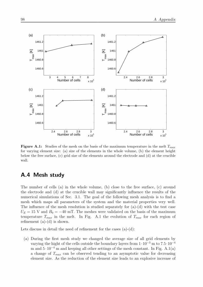
98 A Appendix
3 4 5 6 7 8
x 105
1460.6
1460.8
1461
1461.2
Number of cells
Tm
ax [K
](a)
2.4 2.6 2.8 3
x 105
1460.6
1460.8
1461
1461.2
Number of cells
Tm
ax [K
]
(b)
2.4 2.6 2.8 3
x 105
1460.6
1460.8
1461
1461.2
Number of cells
Tm
ax [K
]
(c)
2.4 2.6 2.8 3
x 105
1460.6
1460.8
1461
1461.2
Number of cells
Tm
ax [K
]
(d)
Figure A.1: Studies of the mesh on the basis of the maximum temperature in the melt Tmax
for varying element size: (a) size of the elements in the whole volume, (b) the element heightbelow the free surface, (c) grid size of the elements around the electrode and (d) at the cruciblewall.
A.4 Mesh study
The number of cells (a) in the whole volume, (b) close to the free surface, (c) aroundthe electrode and (d) at the crucible wall may significantly influence the results of thenumerical simulations of Sec. 3.1. The goal of the following mesh analysis is to find amesh which maps all parameters of the system and the material properties very well.The influence of the mesh resolution is studied separately for (a)-(d) with the test caseUE = 15 V and B0 = −40 mT. The meshes were validated on the basis of the maximumtemperature Tmax in the melt. In Fig. A.1 the evolution of Tmax for each region ofrefinement (a)-(d) is shown.
Lets discuss in detail the need of refinement for the cases (a)-(d):
(a) During the first mesh study we changed the average size of all grid elements byvarying the hight of the cells outside the boundary layers from 1 ·10−3 m to 7.5 ·10−4
m and 5 ·10−4 m and keeping all other settings of the mesh constant. In Fig. A.1(a)a change of Tmax can be observed tending to an asymptotic value for decreasingelement size. As the reduction of the element size leads to an explosive increase of

A.4 Mesh study 99
the overall cell number and therefore to an explosive increase of the computationaltime we have chosen an average element size of 7.5 · 10−4 m for the final mesh.
(b) As we expected large temperature gradients at the surface of the melt, we comparedmeshes with boundary layers thicknesses ranging from 8 · 10−3 m to 1 · 10−2 m anda thickness of the smallest cells ranging from 1 · 10−3 m to 4 · 10−4 m, 2 · 10−4 mand 1 · 10−4 m. For this mesh studies we observed the maximum variations in Tmax
as shown in Fig. A.1(b). But again the rate of changes also reduces with reducingelement size and tends to an asymptotic value. As the ratio width/hight of anelement should not exceed 1/10 [19], and the average width of a surface element is1 · 10−3 m we have chosen an element thickness of 1 · 10−4 m.
(c) The need to study the influence of the grid size around the electrode is twofold. First,the electric current flowing from one rod electrode to another meets the greatestelectric current density in the immediate vicinity of the electrodes. Consequently,these regions acquire high local temperatures. As the electrical conductivity isincreasing expontially with the temperature, a good mapping of the property lawσ(T ) requires a fine mesh in hot regions of the melt. Furthermore, at the squarededges of the electrode the exact solution of the Laplace Eq. (3.10) has a singularity.The numerics yields in high values of ∇φ at the edges which require a refinement aswell [38]. We have compared a mesh without boundary layer around the electrodewith two meshes with a boundary layer thickness of δ = 5 · 10−3 m and the smallestcell sizes of 4 · 10−4 m and 2 · 10−4 m. A significant change can be observed if wecompare meshes without boundary layer. A refinement of the boundary layer cellsleads to an rapid convergence towards an asymptotic value, see Fig. A.1(c).
(d) The Prandtl Number Pr, which describes the ratio between thermal and viscousdiffusion, is for glass melts about Pr ≈ 100. Furthermore, it is a measure of the ratiobetween the velocity boundary layer thickness δs and the temperature boundarylayer thickness δt. As the relation Pr1/2 ∼ (δs/δt) is valid for laminar flow at aflat plate [77], we can expect that δt is about ten times smaller than δs. Due to thesmall dimensions we do not expect free flow and have the smallest velocity boundarylayer thickness between the electrode and the crucible wall with δs = 8.5 · 10−3 m,and hence at theoretical thermal boundary layer thickness of δt = 8.5 · 10−4 m. Aproper resolution with 10 cells requires an average cell thickness of 8.5 · 10−5 m. Westudied the influence of the resolution of the thermal boundary layer by refining thethickness the smallest cells at the crucible wall from 4 · 10−4, 2 · 10−4, 1 · 10−4 to5 · 10−5. The results in Fig. A.1(d) show that the influence of the boundary layerthickness at the crucible wall is negligible.
Fig. A.2 shows the mesh of the crucible geometry (Figs. 3.1, 3.2), which we finally usedfor the numerical simulations.
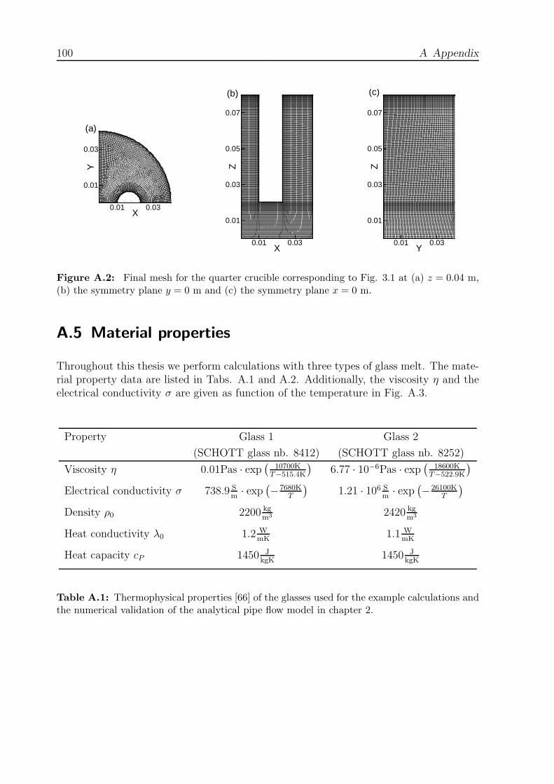
100 A Appendix
X
Y
0.01 0.03
0.01
0.03
(a)
X
Z0.01 0.03
0.01
0.03
0.05
0.07
(b)
Y
Z
0.01 0.03
0.01
0.03
0.05
0.07
(c)
Figure A.2: Final mesh for the quarter crucible corresponding to Fig. 3.1 at (a) z = 0.04 m,(b) the symmetry plane y = 0 m and (c) the symmetry plane x = 0 m.
A.5 Material properties
Throughout this thesis we perform calculations with three types of glass melt. The mate-rial property data are listed in Tabs. A.1 and A.2. Additionally, the viscosity η and theelectrical conductivity σ are given as function of the temperature in Fig. A.3.
Property Glass 1 Glass 2
(SCHOTT glass nb. 8412) (SCHOTT glass nb. 8252)
Viscosity η 0.01Pas · exp(
10700KT−515.4K
)6.77 · 10−6Pas · exp
(18600K
T−522.9K
)
Electrical conductivity σ 738.9 Sm· exp
(−7680K
T
)1.21 · 106 S
m· exp
(−26100K
T
)
Density ρ0 2200 kgm3 2420 kg
m3
Heat conductivity λ0 1.2 WmK
1.1 WmK
Heat capacity cP 1450 JkgK
1450 JkgK
Table A.1: Thermophysical properties [66] of the glasses used for the example calculations andthe numerical validation of the analytical pipe flow model in chapter 2.

A.5 Material properties 101
Property Glass 3
(47.7%BaO-20.0%B2O3-27.1%SiO2-5.2%FeO2)
Viscosity η 9.92 · 10−2Pas · exp(
1046.20KT−1033.41K
)
Electrical conductivity σ 1.74 · 106 Sm· exp
(−20300K
T
)
Density ρ 3931.5 kgm3 − 0.3953 kg
m3K· T
Heat conductivity λ 2 · 10−6 WmK3 · T 2 − 3.2 · 10−3 W
mK2 · T + 2.68 WmK
Heat capacity cP 1285 JkgK
Table A.2: Thermophysical properties of the composition 47.7%BaO-20.0%B2O3-27.1%SiO2-5.2FeO2 (all data in mass%) which are used for the three-dimensional simulations and theone-dimensional convection model in chapter 3.
1300 1400 1500 1600 1700
100
102
104
106
T [K]
η [P
as]
Glass 1Glass 2Glass 3
(a)
1300 1400 1500 1600 1700
0
2
4
6
8
10
12
T [K]
σ [S
/m]
Glass 1Glass 2Glass 3
(b)
Figure A.3: (a) Viscosity η and (b) electrical conductivity σ as function of the temperature Tfor the three glass melt compositions we consider in this thesis. The material property laws aregiven in Tabs. A.1 and A.1.

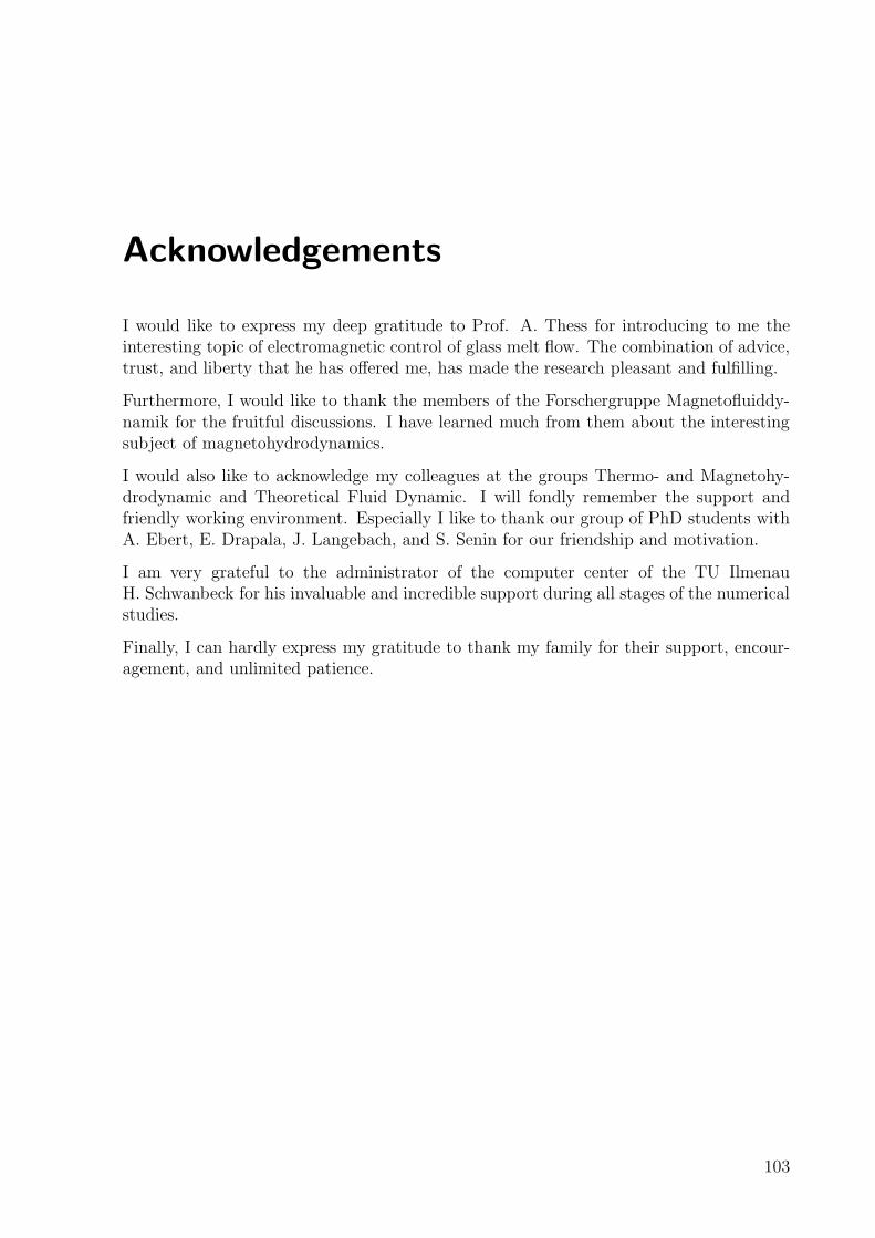
Acknowledgements
I would like to express my deep gratitude to Prof. A. Thess for introducing to me theinteresting topic of electromagnetic control of glass melt flow. The combination of advice,trust, and liberty that he has offered me, has made the research pleasant and fulfilling.
Furthermore, I would like to thank the members of the Forschergruppe Magnetofluiddy-namik for the fruitful discussions. I have learned much from them about the interestingsubject of magnetohydrodynamics.
I would also like to acknowledge my colleagues at the groups Thermo- and Magnetohy-drodynamic and Theoretical Fluid Dynamic. I will fondly remember the support andfriendly working environment. Especially I like to thank our group of PhD students withA. Ebert, E. Drapala, J. Langebach, and S. Senin for our friendship and motivation.
I am very grateful to the administrator of the computer center of the TU IlmenauH. Schwanbeck for his invaluable and incredible support during all stages of the numericalstudies.
Finally, I can hardly express my gratitude to thank my family for their support, encour-agement, and unlimited patience.
103


![Design of Extrusion Dies · the die exit.[6] The design of extrusion dies today is facilitated by computer-based simulation tools. The flow of non-Newtonian fluids through complex](https://static.fdocuments.in/doc/165x107/5e8ef4c4b0aef441777b442b/design-of-extrusion-the-die-exit6-the-design-of-extrusion-dies-today-is-facilitated.jpg)


