2010/80

!

Voting over piece-wise linear tax methods

Juan D. Moreno-Ternero

Center for Operations Research and Econometrics

Voie du Roman Pays, 34

B-1348 Louvain-la-Neuve Belgium

http://www.uclouvain.be/core

D I S C U S S I O N P A P E R

CORE DISCUSSION PAPER 2010/80

Voting over piece-wise linear tax methods

Juan D. MORENO-TERNERO1

December 2010

Abstract

We analyze the problem of choosing the most appropriate method for apportioning taxes in a democracy. We consider a simple theoretical model of taxation and restrict our attention to piece-wise linear tax methods, which are almost ubiquitous in advanced democracies world- wide. We show that if we allow agents to vote for any method within a rich domain of piece-wise linear methods, then a majority voting equilibrium exists. Furthermore, if most voters have income below mean income then each method within the domain can be supported in equilibrium. Keywords: voting, taxes, majority, single-crossing, Talmud.

JEL Classification: D72, H24

1 Universidad de Malaga, Spain; Universidad Pablo de Olavide, Seville, Spain; Université catholique de Louvain, CORE, B-1348 Louvain-la-Neuve, Belgium.

I am most grateful to Oriol Carbonell-Nicolau, Biung-Ghi Ju, François Maniquet, Bernardo Moreno, Ignacio Ortuno-Ortin, Eve Ramaekers, and an anonymous referee for helpful comments and suggestions. I also thank the audiences at the Institute of Food and Resource Economics (University of Copenhagen), the Society of Economic Design Meeting 2009 (Maastricht University), the CORE Weekly Workshop in Welfare Economics (Université catholique de Louvain) and the PAI SEJ426 Research Group (Universidad de Malaga) for many useful discussions. Financial support from the Spanish Ministry of Science and Innovation (ECO2008-03883) and from Junta de Andalucia (P08-SEJ-04154) is gratefully acknowledged.

This paper presents research results of the Belgian Program on Interuniversity Poles of Attraction initiated by the Belgian State, Prime Minister's Office, Science Policy Programming. The scientific responsibility is assumed by the author.

1 Introduction

The primary struggle among citizens in all advanced democracies is over thedistribution of economic resources. Income taxation, besides being a majorsource of state funds, is one of the essential tools for solving such a struggle,which makes it a matter of concern for politicians and economists alike.The search for the perfect income tax structure is (and has been for a longtime) a milestone and even though some consensus has been reached (e.g.,almost all countries in the world use statutory tax schedules specified onlyin terms of the brackets and tax rates) the discussion is far from being over.1

In this paper, we approach this issue from a political economy perspective,upon studying the political process in which tax methods are either chosendirectly by voters, according to majority rule, or via elections in a perfectlyrepresentative democracy.

Academic interest in this area started to emerge after Foley (1967), whoanalyzed the problem of voting over taxes in an endowment economy. Foleyfocused on the case of flat taxes (with or without exemption; and allowingor excluding for the existence of negative taxes) and showed that, for sucha class, there always exists a majority voting equilibrium, i.e., a (flat) taxmethod that cannot be overturned by any other member of the class throughmajority rule.2

In this paper, we plan to focus on the class of piece-wise linear taxmethods (rather than flat taxes) which, as mentioned above, seems to bealmost ubiquitous in advanced democracies worldwide. For such a class,however, Foley’s result does not extend and a majority voting equilibriumfails to exist. In other words, any piece-wise linear tax method can beoverturned by another piece-wise linear tax method through majority rule.This is actually not more than another instance of Condorcet’s paradox ofvoting, which is perhaps best exemplified by the problem of determining thedivision of a cake by majority rule (or, equivalently, tax shares by majority

1In the 2008 US presidential election we had a recent instance of such a discussion.President (then, Senator) Obama proposed a tax plan that would make the tax systemsignificantly more progressive by providing large tax breaks to those at the bottom of theincome scale and raising taxes significantly on upper-income earners. Senator McCaininstead advocated for a tax plan that would make the tax system more regressive, uponproviding relatively little tax relief to those at the bottom of the income scale whileproviding huge tax cuts to households at the very top of the income distribution (e.g.,Burman et al., 2008).

2Foley’s work mostly relies on verbal discussion. A more formal treatment of his model(and some of his results) is provided by Gouveia and Oliver (1996).

1

rule from a given initial distribution of endowments).3

Such a result might lead one to despair of ever achieving a voting equi-librium for any democratic polity. Nevertheless, as Campbell (1975) putsit, majority voting is never allowed to operate by itself without restraintsimposed by constitution and convention. We actually show that if we limitthe class of admissible methods in a meaningful way, albeit not very re-strictive, the existence of a majority voting equilibrium is guaranteed. As amatter of fact, under a mild assumption, we construct the precise equilib-rium for any parameter configuration of the model and show an interestingfeature of it: any tax method within the class can be a majority votingequilibrium, provided the predetermined level of aggregate fiscal revenue isproperly chosen.

The class of admissible methods we consider emerges as a generalizationof a method inspired by the Babylonian Talmud (e.g., O’Neill, 1982; Aumannand Maschler, 1985). The principle underlying behind these methods is toimpose each taxpayer a burden of the same sort as that faced by the wholesociety. Namely, if the overall tax burden is below a certain fraction of theaggregate income, then no taxpayer can pay more than such a fraction ofher gross income. Similarly, if the burden is above a certain fraction ofthe aggregate income, then no taxpayer can pay less than such a fractionof her gross income. The class encompasses a whole non-countable set ofmethods ranging from the “least” progressive (the needs-blind head tax) tothe “most” progressive (the incentives-blind leveling tax) piece-wise lineartax methods. Thus, voters are confronted with a wide variety of choices toselect the best tax method, even if we restrict their options to this class.4

As we shall see later in the text, our modeling choice for this workis somehow unconventional. More precisely, most of the contributions inthis area assume the existence of a continuum (rather than a finite set) oftaxpayers. The main reason for it is twofold. On the one hand, the aim ofmodeling large (rather than small) elections. On the other hand, to allowfor the use of calculus and hence avoid some theoretical problems, such asthose resulting from the non-convexity of the individual voting choice set, orfrom the fact that a change of a vote might make a discrete change in policy(e.g., Alesina and Rosenthal, 1996). Nevertheless, we find some of thoseproblems interesting and hence believe that they should not be dismissed

3Hamada (1973) provides a general treatment regarding why cycling is ubiquitous forthis problem.

4Restricting to a one-parameter family of tax methods in which the parameter reflectsthe degree of progressivity (or regressivity) of the method is a usual course of action intaxation models (e.g., Benabou, 2002).

2

from the outset. That is the main reason why we opt in this paper for adiscrete modeling assumption. Another important reason to do so is theintention to explore the existence of equilibrium in smaller elections, whenthe tax problem refers to collecting a given amount of revenue out of asmall (and hence finite) community. This is also the spirit in part of theliterature to which this paper relates too. A notable instance is Young(1988), which although not concerned with the political economy of incometaxation, could be considered as the seminal paper to analyze the principleof equal sacrifice, and its connections with distributive justice (a recurrenttheme of this paper), in taxation.

The rest of the paper is organized as follows. In Section 2, we intro-duce the model. In Section 3, we provide our main result regarding theexistence of majority voting equilibrium for a large set of piece-wise lineartax methods. In Section 4, we explicitly construct the equilibrium under anadditional condition. Finally, Section 5 concludes.

2 The model

We study taxation problems in a variable population model, first introducedby Young (1988).5 The set of potential taxpayers, or agents, is identified bythe set of natural numbers N. Let N be the set of finite subsets of N, withgeneric element N . For each i ∈ N , let yi ∈ R+ be i’s (taxable) income andy ≡ (yi)i∈N the income profile. A (taxation) problem is a triple consistingof a population N ∈ N , an income profile y ∈ RN

+ , and a tax revenueT ∈ R+ such that

�i∈N yi ≥ T . Let Y ≡

�i∈N yi. To avoid unnecessary

complication, we assume Y =�

i∈N yi > 0. Let DN be the set of taxationproblems with population N and D ≡ ∪N∈NDN .

Given a problem (N, y, T ) ∈ D, a tax profile is a vector x ∈ RN satisfyingthe following three conditions: (i) for each i ∈ N , 0 ≤ xi ≤ yi, (ii)

�i∈N xi =

T and (iii) for each i, j ∈ N , yi ≥ yj implies xi ≥ xj and yi − xi ≥ yj −xj . We refer to (i) as boundedness, (ii) as balancedness and (iii) as orderpreservation. A (taxation) method on D, R : D → ∪N∈NRN , associateswith each problem (N, y, T ) ∈ D a tax profile R (N, y, T ) for the problem.6

5O’Neill (1982) used earlier the same mathematical framework to analyze the prob-lem of adjudicating conflicting claims. Readers are referred to Moulin (2002) or Thom-son (2003) for extensive treatments of diverse problems (such as taxation, conflictingclaims, bankruptcy, cost sharing, or surplus sharing) fitting this framework.

6In essence, the problem under consideration is a distribution problem, in which thetotal amount to be distributed is exogenous, and the issue is to determine methods pro-viding an allocation for each admissible problem. There is another branch of the taxation

3

Instances of methods are the head tax, which distributes the tax burdenequally, provided no agent ends up paying more than her income, the levelingtax, which equalizes post-tax income across agents, provided no agent issubsidized and the flat tax, which equalizes tax rates across agents.

All these methods are instances of piece-wise linear tax methods. For-mally, a piece-wise linear tax method is a method associated to a vectorof brackets, rates and lump-sum levies. For each bracket, a given tax rateis proposed and the corresponding lump-sum levies of the brackets are de-signed so that the schedule moves continuously from one bracket to another.More precisely, a method R is piece-wise linear if for each (N, y, T ) ∈ D thereexist sequences {αj , βj , λj}k

j=1 such that

(i) For each j = 1, . . . , k, αj , λj ∈ R+ and βj ∈ R;

(ii) For each j = 1, . . . , k − 1, λj ≤ λj+1;

(iii) For each j = 1, . . . , k, 0 ≤ αj ≤ 1.

(iv) For each j = 1, . . . , k − 1, αjλj + βj = αj+1λj + βj+1;

(v) For each j = 2, . . . , k, (1− αj)λj−1 ≥ βj ≥ −αjλj−1;

and, for each i ∈ N ,Ri (N, y, T ) = αjyi + βj ,

where j is such that λj−1 ≤ yi ≤ λj .Note that item (iii) above guarantees that every tax schedule has slope

less than one. Item (iv) guarantees that the path of taxes generated by themethod is continuous. Finally, item (v) guarantees that the tax payed byeach agent is neither negative nor higher than her pre-tax income.7

literature in which no reference to the amount of revenue to be raised is made (e.g., Mitraand Ok, 1997). In such a branch, the basic problem is to determine a tax function yieldingthe tax associated to each positive income level. An underlying assumption of the corre-sponding models is to assume the existence of a non-countable set of agents (a reasonableassumption only in the case of arbitrary large populations), which, as mentioned above,allows the use of calculus. A more general approach encompassing both possibilities istaken by Le Breton et al., (1996).

7Alternatively, if we do not impose item (v) in the parameter configuration of themethod R, we shall impose that for each i ∈ N ,

Ri (N, y, T ) = max{0, min{αjyi + βj , yi} = min{yi, max{αjyi + βj , 0},

where j is such that λj−1 ≤ yi ≤ λj , and will also deem the resulting method to be apiece-wise linear method.

4

We will analyze the problem in which agents vote for tax methods ac-cording to majority rule. We assume that voters are self-interested: givena pair of alternatives, a taxpayer votes for the alternative that gives herthe greatest post-tax income. We say that a method R is a majority votingequilibrium for a set of methods S if, for any (N, y, T ) ∈ D, there is no othermethod R� ∈ S such that, y−R� (N, y, T ) > y−R (N, y, T ) for the majorityof voters.

3 The existence of equilibrium

We start this section with a (non-surprising) negative result.

Theorem 1 There is no majority voting equilibrium for the family of piece-wise linear tax methods.

Even though the technical proof of this result might be cumbersome,its logic should be clear. It all amounts to realize that given a piece-wiselinear tax method, one can construct another (piece-wise linear) methodincreasing taxes for a small group of taxpayers and reducing the burden forall the others, while keeping the tax revenue constant. The argument, whichis even valid for two-piece linear methods, is similar to others used in relatedmodels (e.g., Hamada, 1973; Marhuenda and Ortuno-Ortın, 1998).

A caveat is worth mentioning. If more than half of the agents are payingzero taxes, we cannot reduce their burdens and thus the corresponding taxallocation could not be defeated through majority rule by any other alloca-tion. Nevertheless, there is no method guaranteeing that more than half ofthe agents are paying zero taxes for any admissible problem (although therecertainly exist methods doing so for specific problems). The most extremecase would be the leveling tax, which would always be the most preferredmethod by the agent with the lowest income. This method, however, canbe defeated by other piece-wise linear methods in many problems (in which,needless to say, there is not a majority of the population facing a zero taxburden with the leveling tax).

Given the previous result, our aim now shifts to prove the existence ofa majority voting equilibrium for a sufficiently large family of piece-wiselinear tax methods. To do so, we start considering a (piece-wise linear)method inspired by the Babylonian Talmud, implementing an old principleof distributive justice by which each taxpayer should face a burden of thesame sort as that faced by the whole society. More precisely, if the overall taxburden is below one half of the aggregate income (which could be considered

5

as a psychological threshold), then no taxpayer can pay more than such afraction of her gross income. Similarly, if the burden is above one half of theaggregate income, then no taxpayer can pay less than such a fraction of hergross income. Formally,

For all (N, y, T ) ∈ D, and all i ∈ N ,

Ri (N, y, T ) =�

min�yi

2 , λ�

if T ≤ Y2

max�yi

2 , yi − µ�

if T ≥ Y2

where λ > 0 and µ > 0 are chosen so that�

i∈N Ri (N, y, T ) = T .

In the usual parlance of taxation, the “Talmud method” yields two pos-sible types of tax schedules. If the aim is to collect a tax revenue below onehalf of the aggregate income, the tax rate is one half up to some incomelevel (which is endogenously determined), and zero afterwards. If, on thecontrary, the tax revenue is above one half of the aggregate income, the taxrate is one half first and then one. Thus, even though it is a well-justifiedmethod on normative grounds (e.g., Moulin, 2002; Thomson, 2003), it seemsto be quite specific for real-life taxation purposes.

One way of generalizing the Talmud method would be by moving thethreshold (and the tax rate) in the above definition from one half to anyother possible fraction (of the aggregate and individual incomes). In doingso, we would obtain a non-countable set of piece-wise linear methods rangingfrom the leveling tax to the head tax (and having the Talmud method inthe middle).8 Those tax methods would also yield two possible types of taxschedules that could be described similarly to those originating from theTalmud method. More precisely, for tax revenues below a fraction θ of theaggregate income, the tax rate would be θ up to some income level, and zeroafterwards. For tax revenues above such fraction, the tax rate would be θfirst and then one.9

In order to accommodate less restrictive methods too, while preservingthe principle behind the Talmud method, we allow for other minimum andmaximum tax rates, instead of always imposing zero and one for those val-ues. More precisely, we consider tax methods yielding two possible types oftax schedules; namely, for tax revenues below a fraction θ of the aggregateincome, the tax rate would be θ up to some income level, and θmin after-

8The resulting family of methods was studied, in the dual framework of bankruptcyproblems, by Moreno-Ternero and Villar (2006a).

9Note that the flat tax schedules would also be covered by those tax methods, althoughthe flat tax itself could not be considered a method of the resulting family.

6

wards. For tax revenues above such fraction, the tax rate would be θ firstand then θmax. Formally, we have the next definition.

Definition 1 The family of generalized talmudic tax methods {Rθ}θ∈[θmin,θmax].

Let θmin, θmax ∈ [0, 1] be fixed and such that θmin < θmax. For each θ ∈[θmin, θmax], we define the method Rθ as follows. For all (N, y, T ) ∈ D, andall i ∈ N ,

Rθi (N, y, T ) =

�min {θyi,max {θminyi + λ, 0}} if T ≤ θYmax {θyi,min {yi, θmaxyi − µ}} if T ≥ θY

where λ and µ are chosen so that�

i∈N Rθi (N, y, T ) = T .10

In order to illustrate further the above definition, we describe the al-gorithm by which tax burdens are allocated according to the (generalizedtalmudic) method Rθ, as the revenue varies from zero to the aggregate in-come of a given group of taxpayers. More precisely, let y be a given (gross)tax profile such that y1 ≤ y2 ≤ · · · ≤ yn and imagine that the tax revenue Tmoves from 0 to the aggregate income Y =

�ni=1 yi. For T sufficiently small,

the revenue is only financed by n (the taxpayer with the highest income).As T increases, the remaining taxpayers are sequentially asked to pay taxes(once they are able to do so) at the tax rate θmin. This continues until alltaxpayers contribute a θmin fraction of their income. As T increases fromthat point, equal taxation (for the increment) prevails until 1 (the taxpayerwith the lowest income) pays a fraction θ of her income. At that point,1 stops contributing while equal contribution of each (revenue) incrementprevails among the other taxpayers. This process continues (making theremaining taxpayers stop contributing, sequentially, once they contribute aθ fraction of their income) until T = θY . The next increments of T arefaced by n until n − 1 (the taxpayer with the second highest income) cancontribute at the rate θmax, at which point she is invited to do so. As Tincreases from there, the remaining taxpayers are also asked sequentially(but now in the reverse ordering of incomes) to contribute at the rate θmax.Once all agents are contributing at the rate θmax then equal taxation (forthe increment) prevails until 1 contributes with her whole income. Fromthere, equal taxation (for the increment) prevails for the remaining agents,with the proviso that taxpayers contributing their whole income (obviously)stop paying additional increments.

10For ease of exposition, we shall avoid to mention explicitly θmin and θmax, whilereferring to each rule within the family, unless it is specifically needed.

7

It turns out, as the next result shows, that the family of generalizedtalmudic methods described above constitutes a rich domain of piece-wiselinear tax methods for which majority voting equilibrium exists.

Theorem 2 There is a majority voting equilibrium for the family of gener-alized talmudic tax methods.

In order to prove Theorem 2, we need the following lemma, which is inter-esting on its own, and whose proof appears in the appendix.

Lemma 1 Let 0 ≤ θmin ≤ θ1 ≤ θ2 ≤ θmax ≤ 1 and (N, y, T ) ∈ D. Ifn denotes the agent in N with the highest income then Rθ1

n (N, y, T ) ≥Rθ2

n (N, y, T ).

We also need to introduce the following concept:

A method R single-crosses R� if for each (N, y, T ) ∈ D, there exists i ∈ Nsuch that one of the following statements holds:

(i) Rj(N, y, T ) ≤ R�j(N, y, T ) for all j such that yj ≤ yi and Rj(N, y, T ) ≥

R�j(N, y, T ) for all j such that yj ≥ yi.

(ii) Rj(N, y, T ) ≥ R�j(N, y, T ) for all j such that yj ≤ yi and Rj(N, y, T ) ≤

R�j(N, y, T ) for all j such that yj ≥ yi.

The single-crossing property allows one to separate those agents whobenefit from the application of one method or the other, depending on therank of their incomes. It is well known that a sufficient condition for theexistence of a majority voting equilibrium is that voters exhibit intermedi-ate preferences over the set of alternatives (e.g., Gans and Smart, 1996).Thus, as we assume that voters are self-interested and therefore simply voteaccording to the post-tax incomes that methods offer to them, it sufficesto show that, for any pair of values θ1, θ2 ∈ [θmin, θmax], Rθ1 single-crossesRθ2 . To do so, let 0 ≤ θmin ≤ θ1 ≤ θ2 ≤ θmax ≤ 1, with θmin < θmax, and(N, y, T ) ∈ D be given. For ease of exposition, assume that N = {1, . . . , n}and y1 ≤ y2 ≤ · · · ≤ yn. Then, it is enough to show that there exists somei∗ ∈ N such that:

(i) Rθ1i (N, y, T ) ≤ Rθ2

i (N, y, T ) for all i = 1, ..., i∗ and(ii) Rθ1

i (N, y, T ) ≥ Rθ2i (N, y, T ) for all i = i∗ + 1, ..., n.

We distinguish five cases:Case 1: 0 ≤ T ≤ θmin(Y − ny1).

8

In this case, the single-crossing property trivially follows as Rθ1 (N, y, T ) ≡Rθ2 (N, y, T ).

Case 2: θmin(Y − ny1) < T ≤ θ1Y .In this case, by the definition of the family of generalized talmudic meth-

ods, Rθj

i (N, y, T ) = min{θjyi, θminyi +λj}, for all i ∈ N and j = 1, 2, whereλ1 and λ2 are chosen so as to achieve feasibility. Let r1 be the smallestnon-negative integer in {0, ..., n} such that T ≤ θ1(

�r1i=1 yi) + (n− r1)(θ1 −

θmin)yr1+1 and r2 the smallest non-negative integer in {0, ..., n} such thatT ≤ θ2(

�r2i=1 yi) + (n − r2)(θ2 − θmin)yr2+1. It is straightforward to show

that r2 ≤ r1. Thus,

Rθ1 (N, y, T ) = (θ1y1, ..., θ1yr2 , ..., θ1yr1 , θminyr1+1 + λ1, ..., θminyn + λ1), andRθ2 (N, y, T ) = (θ2y1, ..., θ2yr2 , θminyr2+1 + λ2, ..., θminyr1+1 + λ2, ..., θminyn + λ2),

where λ1 =T−θ1(

Pr1i=1 yi)−θmin

“Pni=r1+1 yi

”

n−r1and λ2 =

T−θ2(Pr2

i=1 yi)−θmin

“Pni=r2+1 yi

”

n−r2.

Consequently, Rθ1i (N, y, T ) ≤ Rθ2

i (N, y, T ) for all i = 1, ..., r2 and, byLemma 1, Rθ1

i (N, y, T ) ≥ Rθ2i (N, y, T ) for all i = r1 + 1, ..., n. To con-

clude the proof of this case, we distinguish three subcases:Subcase 2.1: λ2 + θminyr2+1 < θ1yr2+1.Then, i∗ = r2 + 1 and the single-crossing property holds.Subcase 2.2: λ2 + θminyr1 ≥ θ1yr1 .Then, i∗ = r1 + 1 and the single-crossing property holds.Subcase 2.3: λ2 ∈ [(θ1 − θmin)yr2+1, (θ1 − θmin)yr1 ].Then, there exists some k ∈ {r2+1, ..., r1−1} such that (θ1−θmin)yk+1 >

λ2 ≥ (θ1− θmin)yk. Thus, i∗ = k + 1 and the single-crossing property holds.Case 3: θ1Y < T < θ2Y .By the definition of the family of generalized talmudic methods, Rθ1

i (N, y, T ) =max{θ1yi, θmaxyi−µ} and Rθ2

i (N, y, T ) = min{θ2yi, θminyi+λ} for all i ∈ N ,where µ and λ are chosen so as to achieve feasibility. Let r1 be the small-est non-negative integer in {0, ..., n − 1} such that T ≥ θ1Y + (θmax −θ1)((

�ni=r1+1 yi)− (n− r1)yr1+1). Furthermore, let r2 be the smallest non-

negative integer in {0, ..., n− 1} such that T ≤ θ2(�r2

i=1 yi) + (n− r2)(θ2 −θmin)yr2+1. It is straightforward to show that r2 ≤ r1. Thus,

Rθ1 (N, y, T ) = (θ1y1, ..., θ1yr1 , θmaxyr1+1 − µ, ..., θmaxyn − µ), andRθ2 (N, y, T ) = (θ2y1, ..., θ2yr2 , θminyr2+1 + λ, ..., θminyn + λ),

where λ =T−θ2(

Pr2i=1 yi)−θmin

“Pni=r2+1 yi

”

n−r2and µ =

θ1(Pr1

i=1 yi)+θmax

“Pni=r1+1 yi

”−T

n−r1.

Consequently, Rθ1i (N, y, T ) ≤ Rθ2

i (N, y, T ) for all i = 1, ...,min{r1, r2}. Toconclude the proof of this case, we distinguish two subcases:

9

Subcase 3.1: r1 ≥ r2.Then, Rθ1

i (N, y, T ) ≤ Rθ2i (N, y, T ) for all i = 1, ..., r2. By Lemma 1,

Rθ1n (N, y, T ) ≥ Rθ2

n (N, y, T ). Let k be the smallest non-negative integer inN such that Rθ1

k (N, y, T ) ≥ Rθ2k (N, y, T ).11 Two options are then open.

If k ≥ r1 + 1, then θmaxyk − µ = Rθ1k (N, y, T ) ≥ Rθ2

k (N, y, T ) = λ +θminyk. Thus, (θmax − θmin)yk� ≥ µ + λ for all k� = k, ..., n, or equivalently,Rθ1

k� (N, y, T ) ≥ Rθ2k� (N, y, T ) for all k� = k, ..., n and the single-crossing

property follows. If, on the other hand, r2 + 1 ≤ k ≤ r1, then θ1yk =Rθ1

k (N, y, T ) ≥ Rθ2k (N, y, T ) = λ + θminyk. Thus, (θ1 − θmin)yk� ≥ λ for all

k� = k, ..., n. In particular, Rθ1k� (N, y, T ) ≥ Rθ2

k� (N, y, T ) for all k� = k, ..., r1.Now, as Rθ1

r1+1 (N, y, T ) = θmaxyr1+1−µ ≥ θ1yr1+1 ≥ λ+θminyr1+1 we obtainthat µ + λ ≤ (θmax − θmin)yr1+1 ≤ (θmax − θmin)yk� for all k� = r1 + 1, ..., n.As a result, Rθ1

k� (N, y, T ) ≥ Rθ2k� (N, y, T ) for all k� = k, ..., n, and the single-

crossing property follows.Subcase 3.2: r1 < r2.Then, Rθ1

i (N, y, T ) ≤ Rθ2i (N, y, T ) for all i = 1, ..., r1. Furthermore, by

Lemma 1, Rθ1n (N, y, T ) ≥ Rθ2

n (N, y, T ). Let k be the smallest non-negativeinteger in N such that Rθ1

k (N, y, T ) ≥ Rθ2k (N, y, T ). As before, we have two

options. If k ≥ r2 + 1, then θmaxyk − µ = Rθ1k (N, y, T ) ≥ Rθ2

k (N, y, T ) =λ+θminyk. Thus, yk�(θmax−θmin) ≥ µ+λ for all k� = k, ..., n, or equivalently,Rθ1

k� (N, y, T ) ≥ Rθ2k� (N, y, T ) for all k� = k, ..., n, and the single-crossing

property follows. If, on the other hand, r1 + 1 ≤ k ≤ r2, then, θmaxyk −µ =Rθ1

k (N, y, T ) ≥ Rθ2k (N, y, T ) = θ2yk. Thus, (θmax − θ2)yk� ≥ µ for all

k� = k, ..., n. In particular, Rθ1k� (N, y, T ) ≥ Rθ2

k� (N, y, T ) for all k� = k, ..., r2.Now, as Rθ2

r2+1 (N, y, T ) = λ + θminyr2+1 we know that λ ≤ (θ2− θmin)yr2+1.As θ2yr2+1 ≤ θmaxyr2+1 − µ, it follows that λ + θminyr2+1 ≤ θmaxyr2+1 − µor, equivalently, that λ + µ ≤ (θmax − θmin)yr2+1 ≤ (θmax − θmin)yk� , for allk� = r2+1, ..., n. As a result, Rθ1

k� (N, y, T ) ≥ Rθ2k� (N, y, T ) for all k� = k, ..., n

and the single-crossing property follows.Case 4: θ2Y ≤ T < θmax(Y − ny1) + ny1.In this case, by the definition of the family of generalized talmudic meth-

ods, Rθj

i (N, y, T ) = max{θjyi, θmaxyi−µj}, for all i ∈ N and j = 1, 2, whereµ1 and µ2 are chosen so as to achieve feasibility. Let r1 be the smallest non-negative integer in {0, ..., n} such that T ≥ θ1Y +(θmax−θ1)((

�ni=r1+1 yi)−

(n − r1)yr1+1). Furthermore, let r2 be the smallest non-negative integer in{0, ..., n} such that T ≥ θ2Y + (θmax − θ2)((

�ni=r2+1 yi)− (n− r2)yr2+1). It

11Note that k ≥ r2.

10

is straightforward to show that r2 ≤ r1. Thus,

Rθ1 (N, y, T ) = (θ1y1, ..., θ1yr2 , ..., θ1yr1 , θmaxyr1+1 − µ1, ..., θmaxyn − µ1), andRθ2 (N, y, T ) = (θ2y1, ..., θ2yr2 , θmaxyr2+1 − µ2, ..., θmaxyn − µ2),

where µ1 =θ1(

Pr1i=1 yi)+θmax

“Pni=r1+1 yi

”−T

n−r1and µ2 =

θ2(Pr2

i=1 yi)+θmax

“Pni=r2+1 yi

”−T

n−r2.

By Lemma 1, Rθ1n (N, y, T ) ≥ Rθ2

n (N, y, T ). Thus, µ1 ≤ µ2. Consequently,Rθ1

i (N, y, T ) ≤ Rθ2i (N, y, T ) for all i = 1, ..., r2 and Rθ1

i (N, y, T ) ≥ Rθ2i (N, y, T )

for all i = r1 + 1, ..., n. Now, there are three subcases:Subcase 4.1: µ2 < (θmax − θ1)yr2+1.Then, i∗ = r1 + 1 and the single-crossing property holds.Subcase 4.2: µ2 ≥ (θmax − θ1)yr1 .Then, i∗ = r2 and the single-crossing property holds.Subcase 4.3: µ2 ∈ [(θmax − θ1)yr2+1, (θmax − θ1)yr1 ].Then, there exists some k ∈ {r2+1, ..., r1−1} such that (θmax−θ1)yk+1 >

µ2 ≥ (θmax− θ1)yk. Thus, i∗ = k +1 and the single-crossing property holds.Case 5: T ≥ θmax(Y − ny1) + ny1.In this case, the single-crossing property trivially follows as Rθ1 (N, y, T ) ≡

Rθ2 (N, y, T ).

It is worth mentioning that the above proof of Theorem 2 does notextend to the whole domain of two-piece linear methods. To see this, takethe Talmud method (T ), and the method R

58 , for θmin = 1

4 and θmax = 1.Let (N, y, T ) = ({1, 2, 3}, (4, 16, 20), 15). It is straightforward to show thatT (N, y, T ) =

�2, 13

2 , 132

�, whereas R

58 (N, y, T ) =

�52 , 23

4 , 274

�.

4 Further insights

The proof of Theorem 2 tells us that the majority voting equilibrium for thefamily of generalized talmudic tax methods is precisely the method preferredby the median voter, i.e., the median taxpayer. We now explore furtherthe properties of the equilibrium whose existence has been shown in theprevious section. In what follows, we make the following mild assumption,which reflects a well-established empirical fact in advanced democracies.

Assumption 0. In each taxation problem, the median income is below themean income.

Our next result summarizes the main findings within this section. Toease the exposition of its statement, we assume, without loss of generality,

11

that for each (N, y, T ) ∈ D, N = {1, . . . , n} with n ≥ 3 odd, and y1 ≤y2 ≤ · · · ≤ yn. Let m = n+1

2 denote the median taxpayer of this problem.Furthermore, let Y m =

�nj=m yj − (n−m + 1)ym, and

θ∗ = max�

θmin,T − θmaxY m

Y − Y m

�.

Theorem 3 If Assumption 0 holds, and θminY ≤ T ≤ θmaxY , then Rθ∗

is the majority voting equilibrium for the family of generalized talmudic taxmethods {Rθ}θ∈[θmin,θmax].

Proof. We start with a piece of notation. Let (N, y, T ) ∈ D be given in theconditions described at the statement and let k ∈ N . Let us also considerthe following thresholds:

θk1 = θmax +

T − θmaxY

ny1,

θk2 =

T − θmax(�n

j=k yj − (n− k + 1)yk)�k−1

j=1 yj + (n− k + 1)yk

,

θk3 =

T − θmin(�n

j=k yj − (n− k + 1)yk)�k−1

j=1 yj + (n− k + 1)yk

,

θk4 = θmin +

T − θminY

ny1.

As θminY ≤ T ≤ θmaxY , it is straightforward to show that θk1 ≤ θk

2 ≤ θk3 ≤

θk4 , and that θk

2 ≤ θmax and θk3 ≥ θmin. It can actually be shown, after some

algebraic computations, that

Rθk (N, y, T ) =

θmaxyk + T−θmaxYn if θmin ≤ θ ≤ θk

1

fk(θ) if θk1 ≤ θ ≤ θk

2

θyk if θk2 ≤ θ ≤ θk

3

gk(θ) if θk3 ≤ θ ≤ θk

4

θminyk + T−θminYn if θk

4 ≤ θ ≤ θmax,

(1)

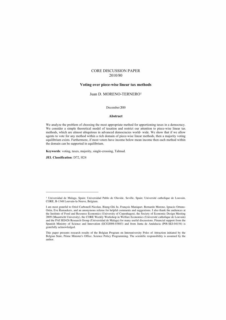
where fk(·) and gk(·) are piece-wise linear decreasing functions.12 A graph-ical illustration appears in Figure 1.

Let k now be the median agent, i.e., k = m. Then, by Assumption 0,it follows that θmaxyk + T−θmaxY

n ≤ θminyk + T−θminYn . As θk

3 ≥ θmin and12Note that θ1

1 = θ12 and θ1

3 = θ14, whereas θn

2 = θn3 . Thus, the taxpayers with the lowest

and highest incomes only have three pieces (two of them constant with respect to θ) intheir preferences.

12

θk2 ≤ θmax, there would be nine possible cases depending of the relative

positions of the remaining θk-thresholds with respect to θmin and θmax. Forour purposes, and thanks to (1), they summarize in just two supra-cases.If θk

2 < θmin then the minimum of Rθk (N, y, T ), and therefore the most

preferred method by agent k, is achieved for θ = θmin. If, otherwise, θk2 ≥

θmin, then the minimum of Rθk (N, y, T ), and therefore the most preferred

method by agent k, is achieved for θ = θm2 . This concludes the proof.

✻

✲

Rθk

θminyk + T−θminYn

θmaxyk + T−θmaxYn

θθ1k θ2

k θ3k θ4

k

❏❏

❏❏❏☞

☞☞☞☞☞☞☞☞☞☞☞☞☞☞❏

❏❏

❏❏

Figure 1: Individual preferences. This figure represents the tax burden pro-posed by the method Rθ, at the problem (N, y, T ), for agent k ∈ N , as a functionof the parameter θ.13

It is straightforward to show that if T = θmaxY then θ∗ = θmax. Thus,the range of θ∗ is the whole interval [θmin, θmax] and, hence, we have thenext corollary.

Corollary 1 Under Assumption 0, any method within the family of gen-eralized talmudic tax methods {Rθ}θ∈[θmin,θmax] can be the majority votingequilibrium for this family, for a given predetermined level of aggregate fis-cal revenue θminY ≤ T ≤ θmaxY .

Theorem 3 provides, under a mild assumption, an explicit expression forthe majority voting equilibrium within the family of generalized talmudic tax

13For simplicity, we consider the second and fourth pieces as linear in the picture,although they are indeed piece-wise linear, as mentioned above.

13

methods, whose existence was shown in Theorem 2, as a function of the dataof the tax problem (namely, the group of taxpayers and the predeterminedlevel of aggregate fiscal revenue). Corollary 1 goes further and shows that,for a given group of taxpayers, and a given method within the family, thereexists a predetermined level of aggregate fiscal revenue for which such amethod is the equilibrium. Thus, if there is freedom to determine the levelof aggregate fiscal revenue to be raised, a given method can be targetedto become the majority voting equilibrium. Another way of reading thiscorollary is as a neutrality condition for the family of generalized talmudictax methods. In other words, the corollary is saying that there is no bias infavor, or against, any of the methods within the family as any of them canarise as an equilibrium.

5 Concluding remarks

We have dealt in this paper with the issue of designing the most appropri-ate income tax. There is a broad consensus worldwide about implementingpiece-wise linear tax methods and therefore we have endorsed such a restric-tion in our (simple) modeling. A key aspect regarding the implementation ofa piece-wise linear tax method is the choice of the corresponding brackets,rates and lump-sum levies. Here we have analyzed such aspect assumingthat the tax parameters are chosen directly by voters according to majorityrule. In spite of the impossibility result saying that if we allow agents tovote freely for any piece-wise linear tax method, no equilibrium can comeout of it, we have obtained two positive results. First, we show that if werestrict the universe in a meaningful way an equilibrium does exist. Sec-ond, we show that, within such a restricted domain, basically any methodcan be the majority voting equilibrium, upon selecting precisely the level ofaggregate fiscal revenue.

Our results also hold for the case of a perfectly representative democ-racy in which tax methods arise as a result of political competition.14 Moreprecisely, assume that there are two parties running in an election and thatcompetition occurs only over tax policies. Given a pair of alternative poli-cies, a taxpayer votes for the one she prefers (i.e., the one that gives herthe greatest post-tax income). If she is indifferent, she votes for each policywith probability one-half. A political equilibrium would then be defined asa Nash equilibrium of the resulting game played by the two parties, where

14See, for instance, Roemer (1999) for a general analysis of the role of political compe-tition in the design of income taxes.

14

they share a common policy space, and in which their payoff functions aretheir probabilities of victory (that obviously depend on their policy choices).Under these conventions, one could easily mimic the results of this paperreplacing the concept of majority rule equilibrium by that of political equi-librium and obtaining that both parties cater to the median voter.

The restriction to piece-wise linear tax methods has not been our onlyassumption in the model. We have also assumed the existence of a finite setof taxpayers, in contrast to most of the related literature, where it seemscustomary to deal with taxes in a calculus framework. We have actuallyeschewed any reference to tax functions and presented our proofs for pre-taxand post-tax vectors. It turns out that simple inequalities, dispensing withany differentiability assumption, have shown to be powerful enough (andmathematically elegant) to prove our results. Our modeling choice has alsoallowed us to analyze interesting features that are normally bypassed in thisarea (such as the effect that a change of a vote might have over policies, or,more generally, the behavior of voters in small elections) because of dealingwith a calculus framework.

We have also imposed a constraint on the tax structure indicating thatthere is a predetermined level of aggregate fiscal revenue that has to beraised. This is a standard feature of both optimal tax models and votingmodels (e.g., Romer, 1975). On the other hand, we have assumed thatlabor is perfectly inelastically supplied. Nevertheless, such assumption couldbe easily relaxed. In a more general model in which agents would havepreferences over consumption and leisure, the preferred tax schedule of themedian voter would also be the majority voting equilibrium, provided bothpreferences and tax schedules satisfy the single-crossing property (e.g., Gansand Smart, 1996). Minor restrictions (e.g., assuming both consumption andleisure are normal goods) would suffice to guarantee that preferences aresingle-crossing, and hence our results would still be relevant in this context.

To conclude, it is worth mentioning that our result regarding the exis-tence of majority voting equilibrium offers as a byproduct an implicationover the distributive power of the methods within the domain being consid-ered. More precisely, and as a consequence of the single-crossing propertythey exhibit, it also holds that the methods within the domain are com-pletely ranked according to the so-called Lorenz dominance criterion, themost fundamental criterion of income inequality.15

15Moreno-Ternero and Villar (2006b) prove this result directly for the case in whichθmin = 0 and θmax = 1.

15

6 Appendix

Proof of Lemma 1We distinguish five cases:Case 1: 0 ≤ T ≤ θmin(Y − ny1).In this case, the statement trivially follows as Rθ1 (N, y, T ) ≡ Rθ2 (N, y, T ).Case 2: θmin(Y − ny1) < T ≤ θ1Y .In this case, by the definition of the family of generalized talmudic meth-

ods, Rθj

i (N, y, T ) = min{θjyi, θminyi +λj}, for all i ∈ N and j = 1, 2, whereλ1 and λ2 are chosen so as to achieve feasibility. Let r1 be the smallestnon-negative integer in {0, ..., n} such that T ≤ θ1(

�r1i=1 yi) + (n− r1)(θ1 −

θmin)yr1+1 and r2 the smallest non-negative integer in {0, ..., n} such thatT ≤ θ2(

�r2i=1 yi) + (n − r2)(θ2 − θmin)yr2+1. It is straightforward to show

that r2 ≤ r1. Thus,

Rθ1 (N, y, T ) = (θ1y1, ..., θ1yr2 , ..., θ1yr1 , θminyr1+1 + λ1, ..., θminyn + λ1), andRθ2 (N, y, T ) = (θ2y1, ..., θ2yr2 , θminyr2+1 + λ2, ..., θminyr1+1 + λ2, ..., θminyn + λ2),

where λ1 =T−θ1(

Pr1i=1 yi)−θmin

“Pni=r1+1 yi

”

n−r1and λ2 =

T−θ2(Pr2

i=1 yi)−θmin

“Pni=r2+1 yi

”

n−r2.

Consequently, Rθ1i (N, y, T ) ≤ Rθ2

i (N, y, T ) for all i = 1, ..., r2. Assume,by contradiction, that Rθ1

n (N, y, T ) < Rθ2n (N, y, T ), i.e., λ1 < λ2. Then,

Rθ1i (N, y, T ) < Rθ2

i (N, y, T ) for all i = r1 + 1, ..., n. Finally, let k ∈{r2+1, ..., r1−1}. Then, Rθ1

k (N, y, T ) = θ1yk ≤ θminyk+λ1 < θminyk+λ2 =Rθ2

k (N, y, T ). Thus,

T =n�

i=1

Rθ1i (N, y, T ) <

n�

i=1

Rθ2i (N, y, T ) = T,

which represents a contradiction.Case 3: θ1Y < T < θ2Y .By the definition of the family of generalized talmudic methods, Rθ1

i (N, y, T ) =max{θ1yi, θmaxyi−µ} and Rθ2

i (N, y, T ) = min{θ2yi, θminyi+λ} for all i ∈ N ,where µ and λ are chosen so as to achieve feasibility. Let r1 be the small-est non-negative integer in {0, ..., n − 1} such that T ≥ θ1Y + (θmax −θ1)((

�ni=r1+1 yi)− (n− r1)yr1+1). Furthermore, let r2 be the smallest non-

negative integer in {0, ..., n− 1} such that T ≤ θ2(�r2

i=1 yi) + (n− r2)(θ2 −θmin)yr2+1. It is straightforward to show that r2 ≤ r1. Thus,

Rθ1 (N, y, T ) = (θ1y1, ..., θ1yr1 , θmaxyr1+1 − µ, ..., θmaxyn − µ), andRθ2 (N, y, T ) = (θ2y1, ..., θ2yr2 , θminyr2+1 + λ, ..., θminyn + λ),

16

where λ =T−θ2(

Pr2i=1 yi)−θmin

“Pni=r2+1 yi

”

n−r2and µ =

θ1(Pr1

i=1 yi)+θmax

“Pni=r1+1 yi

”−T

n−r1.

Consequently, Rθ1i (N, y, T ) ≤ Rθ2

i (N, y, T ) for all i = 1, ...,min{r1, r2}. As-sume, by contradiction, that Rθ1

n (N, y, T ) < Rθ2n (N, y, T ), i.e., (θmax −

θmin)yn < µ + λ. It follows from here that (θmax − θmin)yk < µ + λ forall k ∈ N . Thus, Rθ1

i (N, y, T ) < Rθ2i (N, y, T ) for all i = max{r1, r2}, ..., n.

Finally, let k ∈ {min{r1, r2}+ 1, ...,max{r1, r2}− 1}.If r1 < r2 then Rθ1

k (N, y, T ) = θmaxyk−µ ≥ θ1yk whereas Rθ2k (N, y, T ) =

θ2yk ≤ θminyk + λ. Thus,

Rθ1k (N, y, T ) = θmaxyk − µ

< θmaxyk − (θmax − θmin)yn + λ

≤ θmaxyk − θmaxyn + θ2yn

≤ θ2yk

= Rθ2k (N, y, T ) .

If r1 > r2 then Rθ1k (N, y, T ) = θ1yk ≥ θmaxyk−µ whereas Rθ2

k (N, y, T ) =λ + θminyk ≤ θ2yk. Thus,

Rθ1k (N, y, T ) = θ1yk

≤ θ1yn − θmin(yn − yk)≤ (θmax − θmin)yn − µ

< θminyk + λ

= Rθ2k (N, y, T ) .

We have therefore shown that, in any case, Rθ1k (N, y, T ) < Rθ2

k (N, y, T )for all k ∈ {min{r1, r2}+ 1, ...,max{r1, r2}− 1}. Thus,

T =n�

i=1

Rθ1i (N, y, T ) <

n�

i=1

Rθ2i (N, y, T ) = T,

which represents a contradiction.Case 4: θ2Y ≤ T < θmax(Y − ny1) + ny1.In this case, by the definition of the family of generalized talmudic meth-

ods, Rθj

i (N, y, T ) = max{θjyi, θmaxyi−µj}, for all i ∈ N and j = 1, 2, whereµ1 and µ2 are chosen so as to achieve feasibility. Let r1 be the smallest non-negative integer in {0, ..., n} such that T ≥ θ1Y +(θmax−θ1)((

�ni=r1+1 yi)−

(n − r1)yr1+1). Furthermore, let r2 be the smallest non-negative integer in

17

{0, ..., n} such that T ≥ θ2Y + (θmax − θ2)((�n

i=r2+1 yi)− (n− r2)yr2+1). Itis straightforward to show that r2 ≤ r1. Thus,

Rθ1 (N, y, T ) = (θ1y1, ..., θ1yr2 , ..., θ1yr1 , θmaxyr1+1 − µ1, ..., θmaxyn − µ1),Rθ2 (N, y, T ) = (θ2y1, ..., θ2yr2 , θmaxyr2+1 − µ2, ..., θmaxyn − µ2),

where µ1 =θ1(

Pr1i=1 yi)+θmax

“Pni=r1+1 yi

”−T

n−r1and µ2 =

θ2(Pr2

i=1 yi)+θmax

“Pni=r2+1 yi

”−T

n−r2.

Consequently, Rθ1i (N, y, T ) ≤ Rθ2

i (N, y, T ) for all i = 1, ..., r2. Assume,by contradiction, that Rθ1

n (N, y, T ) < Rθ2n (N, y, T ), i.e., µ1 > µ2. Then,

Rθ1i (N, y, T ) < Rθ2

i (N, y, T ) for all i = r1 + 1, ..., n. Finally, let k ∈{r2 + 1, ..., r1 − 1}. Then, Rθ1

k (N, y, T ) = θ1yk ≤ θ2yk ≤ θmaxyk − µ2 =Rθ2

k (N, y, T ). Thus,

T =n�

i=1

Rθ1i (N, y, T ) <

n�

i=1

Rθ2i (N, y, T ) = T,

which represents a contradiction.Case 5: T ≥ θmax(Y − ny1) + ny1.In this case, the statement trivially follows as Rθ1 (N, y, T ) ≡ Rθ2 (N, y, T ).

References

[1] Alesina, A., Rosenthal, H., 1996, A Theory of Divided Government,Econometrica 64, 1311-1341.

[2] Aumann RJ, Maschler M, 1985, Game theoretic analysis of abankruptcy problem from the Talmud, Journal of Economic Theory36, 195-213.

[3] Benabou, R., 2002, Tax and Education Policy in a Heterogeneous AgentEconomy: What Levels of Redistribution Maximize Growth and Effi-ciency? Econometrica 70, 481-517.

[4] Burman, L., Khitatrakun, S., Leiserson. G., Rohaly, J., Toder, E.,Williams, B., 2008, An Updated Analysis of the 2008 Presidential Can-didates’ Tax Plans. Tax Policy Center. Urban Institute and BrookingsInstitution.

[5] Campbell, D., 1975, Income distribution under majority rule and alter-native taxation criteria, Public Choice 22, 23-35.

18

[6] Foley, D., 1967, Resource allocation and the public sector, Yale Eco-nomic Essays 7, 45-98.

[7] Gans, J. S., Smart, M., 1996, Majority voting with single-crossing pref-erences, Journal of Public Economics 59, 219-237.

[8] Gouveia, M., Oliver, D., 1996, Voting over flat taxes in an endowmenteconomy, Economics Letters 50, 251-258

[9] Hamada, K., 1973, A Simple majority rule on the Distribution of In-come, Journal of Economic Theory 6, 243-264.

[10] Le Breton, M., Moyes, P., Trannoy, A., 1996, Inequality Reducing Prop-erties of Composite Taxation, Journal of Economic Theory 69, 71-103.

[11] Marhuenda F., Ortuno-Ortin, I., 1998, Income taxation, uncertaintyand stability. Journal of Public Economics 67, 285-300.

[12] Mitra, T., Ok, E., 1997, On the equitability of progressive taxation,Journal of Economic Theory 73, 316-334.

[13] Moreno-Ternero J, Villar A., 2006a, The TAL-family of rules forbankruptcy problems. Social Choice and Welfare 27, 231-249.

[14] Moreno-Ternero J, Villar A., 2006b, On the relative equitability of afamily of taxation rules. Journal of Public Economic Theory 8, 283-291.

[15] Moulin, H., 2002, Axiomatic cost and surplus-sharing, in: K. Arrow, A.Sen, K. Suzumura, (Eds.), The Handbook of Social Choice and Welfare,Vol.1, 289-357, North-Holland.

[16] O’Neill, B., 1982, A problem of rights arbitration from the Talmud,Mathematical Social Sciences 2, 345-371.

[17] Romer, T., 1975, Individual welfare, majority voting, and the propertiesof a linear income tax, Journal of Public Economics 4, 163-186.

[18] Roemer, J., 1999, The democratic political economy of progressive in-come taxation, Econometrica 67, 1-19.

[19] Thomson, W., 2003, Axiomatic and game-theoretic analysis ofbankruptcy and taxation problems: a survey, Mathematical Social Sci-ences 45, 249-297.

[20] Young P., 1988, Distributive justice in taxation, Journal of EconomicTheory 44, 321-335.

19

Recent titles CORE Discussion Papers

2010/41. Pierre PESTIEAU and Maria RACIONERO. Tagging with leisure needs. 2010/42. Knud J. MUNK. The optimal commodity tax system as a compromise between two objectives. 2010/43. Marie-Louise LEROUX and Gregory PONTHIERE. Utilitarianism and unequal longevities: A

remedy? 2010/44. Michel DENUIT, Louis EECKHOUDT, Ilia TSETLIN and Robert L. WINKLER. Multivariate

concave and convex stochastic dominance. 2010/45. Rüdiger STEPHAN. An extension of disjunctive programming and its impact for compact tree

formulations. 2010/46. Jorge MANZI, Ernesto SAN MARTIN and Sébastien VAN BELLEGEM. School system

evaluation by value-added analysis under endogeneity. 2010/47. Nicolas GILLIS and François GLINEUR. A multilevel approach for nonnegative matrix

factorization. 2010/48. Marie-Louise LEROUX and Pierre PESTIEAU. The political economy of derived pension

rights. 2010/49. Jeroen V.K. ROMBOUTS and Lars STENTOFT. Option pricing with asymmetric

heteroskedastic normal mixture models. 2010/50. Maik SCHWARZ, Sébastien VAN BELLEGEM and Jean-Pierre FLORENS. Nonparametric

frontier estimation from noisy data. 2010/51. Nicolas GILLIS and François GLINEUR. On the geometric interpretation of the nonnegative

rank. 2010/52. Yves SMEERS, Giorgia OGGIONI, Elisabetta ALLEVI and Siegfried SCHAIBLE.

Generalized Nash Equilibrium and market coupling in the European power system. 2010/53. Giorgia OGGIONI and Yves SMEERS. Market coupling and the organization of counter-

trading: separating energy and transmission again? 2010/54. Helmuth CREMER, Firouz GAHVARI and Pierre PESTIEAU. Fertility, human capital

accumulation, and the pension system. 2010/55. Jan JOHANNES, Sébastien VAN BELLEGEM and Anne VANHEMS. Iterative regularization

in nonparametric instrumental regression. 2010/56. Thierry BRECHET, Pierre-André JOUVET and Gilles ROTILLON. Tradable pollution permits

in dynamic general equilibrium: can optimality and acceptability be reconciled? 2010/57. Thomas BAUDIN. The optimal trade-off between quality and quantity with uncertain child

survival. 2010/58. Thomas BAUDIN. Family policies: what does the standard endogenous fertility model tell us? 2010/59. Nicolas GILLIS and François GLINEUR. Nonnegative factorization and the maximum edge

biclique problem. 2010/60. Paul BELLEFLAMME and Martin PEITZ. Digital piracy: theory. 2010/61. Axel GAUTIER and Xavier WAUTHY. Competitively neutral universal service obligations. 2010/62. Thierry BRECHET, Julien THENIE, Thibaut ZEIMES and Stéphane ZUBER. The benefits of

cooperation under uncertainty: the case of climate change. 2010/63. Marco DI SUMMA and Laurence A. WOLSEY. Mixing sets linked by bidirected paths. 2010/64. Kaz MIYAGIWA, Huasheng SONG and Hylke VANDENBUSSCHE. Innovation, antidumping

and retaliation. 2010/65. Thierry BRECHET, Natali HRITONENKO and Yuri YATSENKO. Adaptation and mitigation

in long-term climate policies. 2010/66. Marc FLEURBAEY, Marie-Louise LEROUX and Gregory PONTHIERE. Compensating the

dead? Yes we can! 2010/67. Philippe CHEVALIER, Jean-Christophe VAN DEN SCHRIECK and Ying WEI. Measuring the

variability in supply chains with the peakedness. 2010/68. Mathieu VAN VYVE. Fixed-charge transportation on a path: optimization, LP formulations

and separation. 2010/69. Roland Iwan LUTTENS. Lower bounds rule!

Recent titles CORE Discussion Papers - continued

2010/70. Fred SCHROYEN and Adekola OYENUGA. Optimal pricing and capacity choice for a public

service under risk of interruption. 2010/71. Carlotta BALESTRA, Thierry BRECHET and Stéphane LAMBRECHT. Property rights with

biological spillovers: when Hardin meets Meade. 2010/72. Olivier GERGAUD and Victor GINSBURGH. Success: talent, intelligence or beauty? 2010/73. Jean GABSZEWICZ, Victor GINSBURGH, Didier LAUSSEL and Shlomo WEBER. Foreign

languages' acquisition: self learning and linguistic schools. 2010/74. Cédric CEULEMANS, Victor GINSBURGH and Patrick LEGROS. Rock and roll bands,

(in)complete contracts and creativity. 2010/75. Nicolas GILLIS and François GLINEUR. Low-rank matrix approximation with weights or

missing data is NP-hard. 2010/76. Ana MAULEON, Vincent VANNETELBOSCH and Cecilia VERGARI. Unions' relative

concerns and strikes in wage bargaining. 2010/77. Ana MAULEON, Vincent VANNETELBOSCH and Cecilia VERGARI. Bargaining and delay

in patent licensing. 2010/78. Jean J. GABSZEWICZ and Ornella TAROLA. Product innovation and market acquisition of

firms. 2010/79. Michel LE BRETON, Juan D. MORENO-TERNERO, Alexei SAVVATEEV and Shlomo

WEBER. Stability and fairness in models with a multiple membership. 2010/80. Juan D. MORENO-TERNERO. Voting over piece-wise linear tax methods.

Books J. GABSZEWICZ (ed.) (2006), La différenciation des produits. Paris, La découverte. L. BAUWENS, W. POHLMEIER and D. VEREDAS (eds.) (2008), High frequency financial econometrics:

recent developments. Heidelberg, Physica-Verlag. P. VAN HENTENRYCKE and L. WOLSEY (eds.) (2007), Integration of AI and OR techniques in constraint

programming for combinatorial optimization problems. Berlin, Springer. P-P. COMBES, Th. MAYER and J-F. THISSE (eds.) (2008), Economic geography: the integration of

regions and nations. Princeton, Princeton University Press. J. HINDRIKS (ed.) (2008), Au-delà de Copernic: de la confusion au consensus ? Brussels, Academic and

Scientific Publishers. J-M. HURIOT and J-F. THISSE (eds) (2009), Economics of cities. Cambridge, Cambridge University Press. P. BELLEFLAMME and M. PEITZ (eds) (2010), Industrial organization: markets and strategies. Cambridge

University Press. M. JUNGER, Th. LIEBLING, D. NADDEF, G. NEMHAUSER, W. PULLEYBLANK, G. REINELT, G.

RINALDI and L. WOLSEY (eds) (2010), 50 years of integer programming, 1958-2008: from the early years to the state-of-the-art. Berlin Springer.

CORE Lecture Series

C. GOURIÉROUX and A. MONFORT (1995), Simulation Based Econometric Methods. A. RUBINSTEIN (1996), Lectures on Modeling Bounded Rationality. J. RENEGAR (1999), A Mathematical View of Interior-Point Methods in Convex Optimization. B.D. BERNHEIM and M.D. WHINSTON (1999), Anticompetitive Exclusion and Foreclosure Through

Vertical Agreements. D. BIENSTOCK (2001), Potential function methods for approximately solving linear programming

problems: theory and practice. R. AMIR (2002), Supermodularity and complementarity in economics. R. WEISMANTEL (2006), Lectures on mixed nonlinear programming.