Copyright Warning &...
166
Copyright Warning & Restrictions The copyright law of the United States (Title 17, United States Code) governs the making of photocopies or other reproductions of copyrighted material. Under certain conditions specified in the law, libraries and archives are authorized to furnish a photocopy or other reproduction. One of these specified conditions is that the photocopy or reproduction is not to be “used for any purpose other than private study, scholarship, or research.” If a, user makes a request for, or later uses, a photocopy or reproduction for purposes in excess of “fair use” that user may be liable for copyright infringement, This institution reserves the right to refuse to accept a copying order if, in its judgment, fulfillment of the order would involve violation of copyright law. Please Note: The author retains the copyright while the New Jersey Institute of Technology reserves the right to distribute this thesis or dissertation Printing note: If you do not wish to print this page, then select “Pages from: first page # to: last page #” on the print dialog screen
Transcript of Copyright Warning &...

Copyright Warning & Restrictions
The copyright law of the United States (Title 17, United States Code) governs the making of photocopies or other
reproductions of copyrighted material.
Under certain conditions specified in the law, libraries and archives are authorized to furnish a photocopy or other
reproduction. One of these specified conditions is that the photocopy or reproduction is not to be “used for any
purpose other than private study, scholarship, or research.” If a, user makes a request for, or later uses, a photocopy or reproduction for purposes in excess of “fair use” that user
may be liable for copyright infringement,
This institution reserves the right to refuse to accept a copying order if, in its judgment, fulfillment of the order
would involve violation of copyright law.
Please Note: The author retains the copyright while the New Jersey Institute of Technology reserves the right to
distribute this thesis or dissertation
Printing note: If you do not wish to print this page, then select “Pages from: first page # to: last page #” on the print dialog screen

The Van Houten library has removed some of the personal information and all signatures from the approval page and biographical sketches of theses and dissertations in order to protect the identity of NJIT graduates and faculty.

ABSTRACT
OPTIMAL TRAIN CONTROL ON VARIOUS TRACK ALIGNMENTSCONSIDERING SPEED AND SCHEDULE ADHERENCE CONSTRAINTS
byKitae Kim
The methodology discussed in this dissertation contributes to the field of transit
operational control to reduce energy consumption. Due to the recent increase in gasoline
cost, a significant number of travelers are shifting from highway modes to public transit,
which also induces higher transit energy consumption expenses.
This study presents an approach to optimize train motion regimes for various
track alignments, which minimizes total energy consumption subject to allowable travel
time, maximum operating speed, and maximum acceleration/deceleration rates. The
research problem is structured into four cases which consist of the combinations of track
alignments (e.g., single vertical alignment and mixed vertical alignment) and the
variation of maximum operating speeds (e.g., constant and variable). The Simulated
Annealing (SA) approach is employed to search for the optimal train control, called
"golden run".
To accurately estimate energy consumption and travel time, a Train Performance
Simulation (TPS) is developed, which replicates train movements determined by a set of
dynamic variables (e,g., duration of acceleration and cruising, coasting position, braking
position, etc.) as well as operational constraints (e.g., track alignment, speed limit,
minimum travel time, etc.)
The applicability of the developed methodology is demonstrated with geographic
data of two real world rail line segments of The New Haven Line of the Metro North
Railroad: Harrison to Rye Stations and East Norwalk to Westport Stations. The results of
optimal solutions and sensitivity analyses are presented. The sensitivity analyses enable a
transit operator to quantify the impact of the coasting position, travel time constraint,
vertical dip of the track alignment, maximum operating speed, and the load and weight of
the train to energy consumption.
The developed models can assist future rail system with Automatic Train Control
(ATC), Automatic Train Operation (ATO) and Positive Train Control (PTC), or
conventional railroad systems to improve the planning and operation of signal systems.
The optimal train speed profile derived in this study can be considered by the existing
signal system for determining train operating speeds over a route.

OPTIMAL TRAIN CONTROL ON VARIOUS TRACK ALIGNMENTSCONSIDERING SPEED AND SCHEDULE ADHERENCE CONSTRAINTS
byKitae Kim
A DissertationSubmitted to the Faculty of
New Jersey Institute of TechnologyIn Partial Fulfillment of the Requirements for the Degree of
Doctor of Philosophy in Civil Engineering
Department of Civil and Environmental Engineering
January 2010

Copyright © 2010 by Kitae Kim
ALL RIGHTS RESERVED

BIOGRAPHICAL SKETCH
Author: Kitae Kim
Degree: Doctor of Philosophy
Date: January 2010
Undergraduate and Graduate Education:
• Doctor of Philosophy in Civil and Environmental Engineering,New Jersey Institute of Technology, Newark, NJ, 2010
• Master of Science in Civil and Environmental Engineering,New Jersey Institute of Technology, Newark, NJ, 2005
• Master of Science in Transportation Planning and Engineering,Polytechnic University, Brooklyn, NY, 2002
• Bachelor of Science in Civil Engineering,Chung-Ang University, Seoul, Korea, 1999
Major: Transportation Engineering
Presentations and Publications:
Kitae Kim and Steven Chien, "Optimal Train Operation for Minimum EnergyConsumption Considering Schedule Adherence", Transportation Research Board89th Annual Meeting, January 2010 (Forthcoming)
Kitae Kim and Steven Chien, "Simulation Analysis of Energy Consumption for VariousTrain Controls and Alignment", Transportation Research Board 88 th AnnualMeeting, January 2009
Steven Chien, Sunil Kumar Daripally, and Kitae Kim, "Development of a ProbabilisticModel to Disseminate Bus Arrival Time", Journal of Advanced Transportation,Vol. 41, No. 2, 2007
Steven Chien, Kitae Kim, and Janice Daniel, "Cost and Benefit Analysis for OptimizedSignal Timing Case Study: New Jersey Route 23", ITE Journal, Vol. 76, No. 10,2006
iv

APPROVAL PAGE
OPTIMAL TRAIN CONTROL ON VARIOUS TRACK ALIGNMENTSCONSIDERING SPEED AND SCHEDULE ADHERENCE CONSTRAINTS
Kitae Kim
Dr, Steven I-Jy Chien, Dissertation Advisor DateProfessor of Civil and Environmental Engineering, NJIT
Dr. Lazar Spasovic, Committee Member DateProfessor of Civil and Environmental Engineering, NJIT
Dr. Athanassios Bladikas, Committee Member DateAssociate Professor of Mechanical and Industrial Engineering, NJIT
Dr. Janice R. Daniel, Committee Member DateAssociate Professor of Civil and Environmental Engineering, NJIT
Dr. Jerome Lutin, Committee Member DateDi nguished Research Professor, Office of the Dean, NCE, NJIT

I would like to dedicate this dissertation to
My beloved wife, Dongwook Oh, who showed me her love, sacrifice, and encouragement
throughout;
My parents, II-Rang Kim and Heeja Ha, who motivated me to study abroad and made all
the sacrifices and my brother Su-young Kim, who gave me encouragement ; and
My mentor, Sun-gak, who always gave me help and advice during my study.

ACKNOWLEDGEMENT
I do greatly appreciate my dissertation advisor, Dr. Steven I-Jy Chien, who constantly
supported, inspired and encouraged me with his insight, dedication and understanding
during my Ph.D. study. Special thanks are given to Dr. Jerome Lutin, Dr. Lazar Spasovic,
Dr. Athanassios Bladikas, and Dr. Janice Daniel for serving as committee members and
providing me with precious suggestions on research and industrial practice, I also express
my appreciation to Mr. Anthony Pincherri at NJ TRANSIT, who provided me with
valuable data for my dissertation.
My fellow graduate students, Dr. Feng-Ming Tsai, Dr, Sungmin Maeng, Dr,
Mingzheng Cao, Mr. Yavuz Ulusoy, Ms. Patricia DiJoseph, and Mr. Jinuk Ha, are
deserving recognition for their support.
I also appreciate all projects sponsored by the New Jersey Department of
Transportation, New Jersey Transit, the National Center for Transportation and Industrial
Productivity, New Jersey Institute of Technology, and the International Road Federation
(IRF) Fellowship Program, which supported my tuition and other financial needs.
vi

TABLE OF CONTENTS
Chapter Page
1 INTRODUCTION 1
1.1 Background 1
1.2 Problem Statement 2
1.3 Objective and Work Scope 4
1,4 Dissertation Organization 6
2 LITERATURE REVIEW 7
2.1 Sustainable Train Operation 7
2.2 Train Performance Simulation (TPS) 12
2.3 Kinematic Models for Train Movement 19
2.3.1 Tractive Effort and Adhesion 19
2.3.2 Train Resistances 22
2,4 Train Control Regimes 26
2.5 Minimization of Energy Consumption for Train Operation 31
2.6 Optimization Algorithms and Heuristics 35
2,7 Summary 38
3 DEVELOPMENT OF TRAIN PERFORMANCE SIMULATION (TPS) 41
3,1 Train Traction Module (TTM) 41
3.2 Track Alignment Module (TAM) 49
3.3 Train Control Module (TCM) 51
4 METHODOLOGY FOR MINIMIZING ENERGY CONSUMPTION 59
vii

TABLE OF CONTENTS(Continued)
Chapter Page
4,1 Model I — SVA and Constant MOS (Case I) 59
4,1.1 System Assumptions 60
4.1.2 Model Formulation 61
4.1.3 Constraints 62
4.1.4 Optimization Model 64
4.2 Model II - SVA and Variable MOS (Case II) 64
4,2.1 System Assumptions 64
4.2,2 Optimization Model 66
4,3 Model III — MVA and Constant MOS (Case III) 66
4.3.1 System Assumptions 67
4.3.2 Optimization Model 69
4.4 Model IV — MVA and Variable MOS (Case IV) 69
4.4.1 System Assumptions 69
4,4.2 Optimization Model 71
4.5 Summary 71
5 SOLUTION METHODS 72
5.1 SVA with Constant MOS (Case I) 72
5,1.1 Train Control for Case I 72
5.1.2 SA for Case II 74
5,1.3 Fitness Function for Case I 81
viii

TABLE OF CONTENTS(Continued)
Chapter Page
5.1.4 Cooling Schedule for Case I 82
5,2 SVA with Variable MOS (Case II) 83
5.2.1 Train Control for Case II 83
5.3 MVA with Constant MOS (Case III) 85
5.4 MVA with Variable MOS (Case IV) 85
5.5 Summary 86
6 CASE STUDY 87
6.1 Optimal Results for Cases I and II 87
6.1.1 SVA with Constant MOS (Case I) 89
6.1,2 SVA with Variable MOS (Case II) 94
6.2 Optimal Results for Cases III and IV 98
6.2.1 The Metro-North Railroad (New Haven Line) 100
6.2.2 MVA with Constant MOS (Case III) 101
6,2.3 MVA with Variable MOS (Case IV) 103
6.3 Results Comparison 105
6.4 Sensitivity Analysis 110
7 CONCLUSIONS AND FUTURE RESEARCH 133
7.1 Conclusions 133
7,2 Future Research 136
REFERENCES 138
ix

LIST OF TABLES
Table Page
1.1 Proposed Work Scope 5
2.1 Indicators of Sustainable Transportation Systems 9
2.2 Review of Train Simulation Models 18
2,3 Summary of Adhesion Coefficients for Various Weather Conditions 22
2,4 Characteristics of Train Resistances 25
2,5 Track Class and Train Speed Limit 26
2,6 Minimization of Energy Consumption for Train Operation Studies 40
3,1 Feasible Train Controls 53
5,1 Simulated Annealing Algorithm 76
6.1 Inputs for Cases I and II 88
6,2 Inputs for Cases III and IV 99
6,3 Track Alignment Geometry and Speed Limit 99
6.4 Results under Optimal Control in Cases I and II 106
6,5 Results of Optimal Control in Case III 106
6,6 Results of Optimal Control in Case IV 107
6,7 Effect of Train Weight on Energy Consumption (Cases III and IV) 128
6,8 Effect of Passenger Load on Energy Consumption (Cases III and IV) 129

LIST OF FIGURES
Figure Page
2.1 Energy Intensities of various transportation modes 10
2.2 Comparison of adhesion coefficients 20
2.3 Adhesion under wet conditions -Shinkansen 200 21
2.4 Four cases of inter-station train control regimes 27
2.5 Train controls of the Tohoku Shinkansen 29
3.1 Longitudinal train forces on a continuously varying track 42
3.2 Adhesion coefficient vs. speed under different rail and wheel conditions 44
3.3 Configuration of a speed profile for a general train control on SVA.... ....,...... 51
3.4 Flow chart of the train performance simulation model 58
4.1 Vertical track alignments between stations A and B 60
4,2 Feasible variable MOS profile on SVA in Case II 65
4.3 Feasible mixed vertical alignment between stations A and B 68
4,4 Feasible variable MOS profile under MVA in Case IV 70
5.1 Train control with four motion regimes 73
5.2 Flow chart of the developed simulated annealing algorithm 80
5.3 Train control under variable MOS scenario 1( Vm1 < Vm2 ) 84
5,4 Train control under variable MOS scenario 2 ( Vm1 > VM2, ) 85
6.1 Tractive effort and speed vs. distance (Level-Case I) 90
6,2 Tractive effort and speed vs. time (Level-Case I) 90
6,3 Tractive effort and speed vs. distance (Convex-Case I). 91
xi

LIST OF FIGURES(Continued)tin ued)
Figures Page
6.4 Tractive effort and speed vs. time (Convex-Case I) 92
6.5 Tractive effort and speed vs. distance (Concave-Case I) 93
6.6 Tractive effort and speed vs, time (Concave-Case I) 93
6.7 Tractive effort and speed vs. distance (Level-Case II) 94
6.8 Tractive effort and speed vs. time (Level-Case II) 95
6,9 Tractive effort and speed vs. distance (Convex-Case II) 96
6.10 Tractive effort and speed vs. time (Convex-Case II) 96
6,11 Tractive effort and speed vs. distance (Concave-Case II) 97
6.12 Tractive effort and speed vs. time (Concave-Case II) 98
6.13 Configuration of Metro North - The New Haven Line 100
6.14 Tractive effort, speed, and vertical track profile vs, distance (Case III) 102
6.15 Tractive effort and speed vs, time (Case III) 102
6,16 Tractive effort, speed, and vertical track profile vs. distance (Case IV) 104
6.17 Tractive effort and speed vs. time (Case IV) 104
6.18 Energy consumption and travel time vs. track alignment and control (Case I) 108
6.19 Energy consumption and travel time vs. track alignment and control (Case II) 109
6.20 Energy consumption and travel time vs. track alignment and control (Case IIIand IV) 110
6.21 Energy consumption and travel time vs. coasting position (Level-Case I) 111
6,22 Energy consumption and travel time vs. coasting position (Convex-Case I) 112
6.23 Energy consumption and travel time vs. coasting position (Concave-Case I) 113
xii

LIST OF FIGURES(Continued)
Figures Page
6.24 Energy consumption and travel time vs. coasting position (Level-Case II).,..,... 114
6,25 Energy consumption and travel time vs. coasting position (Convex-Case II) 115
6.26 Energy consumption and travel time vs. coasting position (Concave-Case II) 116
6,27 Energy consumption and travel time vs, coasting position in Case III 117
6.28 Energy consumption and travel time vs. coasting position in Case IV 117
6,29 Coasting position and energy consumption vs. travel time (Case I) 119
6.30 Coasting position and energy consumption vs, travel time (Case II) 119
6.31 Coasting position and energy consumption vs. travel time (Case III) 120
6.32 Coasting position and energy consumption vs. travel time (Case IV) 121
6.33 Optimal speed profiles vs. maximum allowable travel time 122
6.34 Travel time and energy consumption vs. maximum operating speed (Case I),..... 123
6.35 Travel time and energy consumption vs. maximum operating speed (Case II)..,., 124
6.36 Vertical dip and maximum operating speed vs. energy consumption (Case I)...,. 125
6.37 Vertical dip and maximum operating speed vs. energy consumption (Case II)..,, 126
6,38 Energy consumption vs. vertical dip with threshold MOS (Case I) 127
6.39 Energy consumption vs. coasting speed and position (Case III) 130
6,40 Travel time vs. coasting speed and position (Case III) 130
6.41 Energy consumption vs. coasting speed and position (Case IV) 132
6.42 Travel time vs. coasting speed and position (Case IV) 132

LIST OF SYMBOLS
at Acceleration rate at time t ft/sec2
a ma. Maximum acceleration rate ft/sec2
a Average speed change rate of acceleration ft/sec2
b t Deceleration rate at time t ft/sec2
b. Maximum deceleration rate ft/sec2
b Average speed change rate of deceleration ft/sec2
c , Average speed change rate of 1 st coasting ft/sec2
c2 Average speed change rate of 2 11d coasting ft/sec2
Co Initial control parameter -
Dt Track curvature at time t degree
d i Damping constant lb • sec/ft
Δet Energy consumption rate at time t kWh
E Total energy consumption kWh
AE Energy change kWh
E(S'ω ) Energy at current state kWh
E(S'ω+1) Energy at subsequent state kWh
Fa Adhesive force at time t lbf
F;, tractive effort at time t lbf
Ftp Propulsive force at time t lbf
xiv

FtB(max) Maximum braking force lbf
FL Adhesion-limited braking force lbf
Ftbc Comfort-limited braking force lbf
Fit Tractive effort of the ith car at time t
g Gravitational acceleration (=32.2) ft/sec2
G tTrack grade where the train is running at time t degree
i Index of car in train -
IpInflection point -
j Index of track segment
J Number of time steps for traveling from one station to another -
k, Spring constant lb/ft
kB Boltzmann constant -
K Aerodynamic coefficient -
L Horizontal track length ft
m Train mass lbm
MO Motion regime -
Ma Acceleration regime -
Mb Braking regime -
Mel 1st coasting regime -
Mc2 2nd coasting regime -
xv

Mv Cruising regime -
N Number of cars per train cars/train
n Number of axles per car axels/car
O Index of motion regime -
P Boltzmann probability -
pt Engine horse power at time t hp
q Total number of vertical segment with different grade segments
RtT Total train resistance lbf
RU Unit resistance per axle lbf/ton
S Station spacing ft
Sa Travel distance during accelerating ft
Sb Travel distance during braking ft
Sc1 Travel distance during 1St coasting ft
S, Travel distance during cruising ft
Sc2 Travel distance during 2nd coasting ft
Sb Travel distance during braking ft
S' Neighbor solution in SA kWh
to Acceleration time sec
tc1 1st coasting time sec
t v Cruising time sec
xvi

tc2 2nd coasting time sec
tbBraking time sec
T Total travel time sec
Ttemp Temperature in SA -
u Index of maximum operating speed -
v t Train speed at time t ft/sec
Ay' Increment of train speed from t to t+1 ft/sec
V t Train speed at time t mph
\Tel Speed at 1 St coasting starts mph
Vb Critical speed mph
Vtr Relative speed at time t mph
VMu Maximum operating speed mph
Vtwd Wind speed at time t mph
W Train weight ton
xt Traveled distance at time t ft
yj(xt) Vertical track alignment where x t traveled at time t on ftsegment j
8 Vertical dip/height ft
7 Track transition rate in grade in 100 ft -
/7 Transmission efficiency -
fi t Adhesion coefficient at time t -
xvii

θtiTrack angle to the horizontal degree
θtwd Angle between the directions of wind and train movement degree
P Rotating mass coefficient -
A, Penalty factor -
co Index of iteration number in SA -
xviii

CHAPTER 1
INTRODUCTION
1.1 Background
As a major public transportation mode, rail transit (e.g., light rail and heavy rail systems)
has been widely used in many metropolitan areas in the U.S. Over the years, the total
consumed transit energy increased as the total line haul distance and passengers train
miles of travel increased. It was found that the annual energy usage increased 1.6 percent
for rail freight service and 1.7 percent for rail passenger service from 1995 to 2005. In
2005, 571.4 trillion and 87.6 trillion British Thermal Units (BTU) were respectively
consumed by rail-freight and rail-passenger services. Due to recent increases of gasoline
and other energy costs, many people are expected to shift from highway modes to transit
for their daily travel. This might drastically increase energy expenses to rail transit
suppliers.
According to a report prepared by the US Energy Information Administration
(EIA, 2006), it is expected that transportation energy consumption and energy prices will
continue to increase until 2030. Concerned about rising energy costs, rail transit operators
have implemented energy conservation strategies to maintain sustainability of rail
operations. To improve overall energy efficiency, the San Francisco Bay Area Rapid
Transit District (BART) and the Metropolitan Atlanta Rapid Transit Authority (MARTA)
incorporated regenerative braking energy into their rail system in order to improve
overall energy efficiency. The New York City Transit Authority (NYCTA) has tested
several energy efficient strategies, including coasting, regenerative in-vehicle storage,
and substation battery energy storage (Uher at al,, 1984). Train operations may become
1

2
more efficient by using new technology-oriented improvements such as automatic train
control (ATC), automatic train operation (ATO), and positive train control (PTC), which,
however, are expensive. Moreover, it could be a burden for suppliers to adopt up-and-
coming technologies without assurance of success. Thus, train control can be one viable
approach to reduce expensive energy bills for transit operators.
For most transit operations, train control for stations-to-station movement is
affected by five motion regimes: acceleration, cruising, coasting, braking, and standing.
However, the train control (i.e., driving strategy) used most in rail transit is either for a
flat-out run (e.g., shortest time) or for a single coasting run at a fixed point to achieve
train schedule regulation (Mellitt et al., 1987; Wong and Ho, 2003). Therefore, it is
desirable to develop a dynamic passenger train control model that can reduce energy
consumption considering schedule adherence.
1.2 Problem Statement
Previous studies (Chang and Sim, 1997; Hwang, 1998; Franke et al., 2000; Albecht,
2004) that minimize train energy consumption have been conducted by using different
approaches such as coast control, automatic train operation (ATO), train speed
trajectories, equi-block track system, etc. However, few of them discussed the impact of
vertical or horizontal track alignment on kinematic train forces (e.g., propulsive force,
resistance, adhesion, and acceleration, etc.) and considered alignment as a constant value.
In particular, considering the effect of track alignment variation in optimizing
train energy consumption is very important because the tractive effort (i.e,, propulsive
force or TE) and train resistances are a function of the geometry of the track alignment.
The vertical track alignment may be composed of a series of curves with different radii,

3
which provide a gradual transition from one level to another for smooth riding. There are
two types of parabolic curves used in track alignment design: convex and concave. The
benefits of a convex (vertically dipped) curve that reduces energy consumption and travel
time were discussed by Kim and Schonfeld (1998), while a concave curve favors coasting
operations (Howlett and Pudney, 1995).
A number of previous studies developed optimal train control to reduce energy
consumption, but only a few studies considered the effect of track alignment on train
performance and energy consumption, Furthermore, some approaches for optimizing
energy consumption were developed without considering the effect of track alignment on
TE and resistance, which resulted in the misrepresentation of performance by the models.
It is desirable to develop a sound train control model, which can minimize energy
consumption considering the effect of varying track alignment and train operational
characteristics, such as propulsive force, resistance, and acceleration and deceleration
rates, In addition, the proposed model should be also capable of dealing with a speed
limit, which significantly affects the application of motion regimes (e.g., acceleration,
cruising, coasting, and deceleratiOn). A train speed profile along a route is directly
affected by the speed limit, because of the geometry of track alignment and/or operational
purpose, and by travel time constraints because of scheduled arrival times at downstream
stations, which should be considered while optimizing train control.

4
1.3 Objective and Work Scope
The objective of this study is to develop an analytical model that optimizes train control
to reduce train energy consumption by considering the effect of vertical track alignments,
schedule adherence, and maximum operating speed, which directly affect the incurred TE
and resistances of a train.
While developing an optimal train control, a time-based train performance
simulation (TPS) model will also be developed for demonstrating energy consumption
and travel time induced by a new train control. Therefore, the TPS must accurately
replicate train movements determined by dynamic variables (e.g., duration of acceleration
and cruising, coasting position, braking position, etc.) as well as the primary static
constraints (e.g., track alignment, speed limit, minimum travel time, etc.).
The Maximum Operating Speed (MOS) used in this study is largely divided into
two categories: fixed and variable. The fixed MOS represents a single speed regulating
train speed between two stations, while a variable MOS limit consists of multiple
operating speeds due to track alignment and operational strategy. To develop an optimal
train control by considering the joint impact of track alignment and MOS, four cases are
investigated in this study, The optimal train control is investigated for four cases as
shown in Table 1.1.

Table 1.1 Proposed Work Scope
5
• Case I: Model I is developed to optimize train control for minimum energy
consumption for each of three vertical alignments (e.g., level, convex, and
concave) and fixed maximum operating speed.
• Case II: Model II is enhanced frOm Model I by considering the impact of a
variable maximum operating speed on energy consumption, which is commonly
used in most rail lines.
• Case III: Model III is enhanced from Model I by considering the joint impact of a
mixed vertical alignment (i,e., several curves) and a constant maximum operating
speed.
• Case IV: Model IV is developed by integrating Models II and I1I and considering
the impact of mixed vertical alignments and a variable maximum operating speed.

6
1.4 Dissertation Organization
This dissertation is organized into seven chapters. Chapter 1 introduced the background
of the energy consumption problem for the railroad industry and presents the research
objective and work scope. Chapter 2 summarizes the efforts of previous studies related to
sustainable rail operations, various TPS models, kinematic models for train movement,
and optimal train control for energy savings. Chapter 3 presents the development of the
proposed TPS model, consisting of three modules for handling dynamic train movement
on a continuously varying track with designated motion regimes. Chapter 4 discusses the
development of analytical models used to optimize train control. Chapter 5 introduces the
Simulated Annealing approach to optimize the research problems defined in Cases I
through IV, Chapter 6 presents a numerical example, which demOnstrates the
applicability of the developed TPS model in estimating station-to-station travel time and
energy consumption under various train controls and track alignments. Finally,
conclusions and suggestions for future studies are presented in Chapter 7,

CHAPTER 2
LITERATURE REVIEW
This chapter summarizes the literature review, including sustainable rail operations, train
performance simulation, and methods to search for optimal train control. This chapter is
organized into six sections: Section 2,1 discusses railway energy consumption as a
sustainability indicator; Section 2,2 discusses the review of previous TPS models; Section
2.3 reviews essential kinematic train equations for developing a simulation model;
Section 2.4 discusses the effect of train control on energy consumption; Section 2.5
discuss previous studies of optimizing train energy consumption; Section 2.6 reviews
optimization algorithms and heuristic search methods; and Section 2.7 summarizes the
literature review and establishes the rationale for the model developed by this research.
2.1 Sustainable Train Operation
The sustainability of the transportation system has been receiving a great level of
attention worldwide, In 1987, the United Nations' Brundtland Commission defined
sustainability in the following way: "A sustainable condition for this planet is one in
which there is stability for both social and physical systems, achieved through meeting
the needs of the present without compromising the ability of future generations to meet
their own needs" (United Nations, 1987), The early view of transportation sustainability
focused on fuel use and environmental concerns. More recently, people have been
concerned not only with fuel use and the environment, but also congestion, mobility, and
safety as conditions of sustainability (Richardson, 2000). To assess the sustainability of
an urban transportation system, various indicators were identified (Sinha, 2003). The
7

8
indicators used in his study of transportation sustainability evaluation were developed
based on decennial data (1960 to 1990) from 46 cities in the U.S., Australia, Canada,
Europe, and Asia, which had been established in the study conducted by Kenworthy and
Laube (1999).
Major initiatives in North America and Europe in characterizing the definition
and measurement of transportation sustainability were discussed (Black et al., 2002; Jeon
and Amekudzi, 2005), in which the impact on the economy, environment, safety,
transportation-related, and social well-being were focused and summarized in Table 2.1.

9
Table 2.1 Indicators of Sustainable Transportation Systems
USDOT
USEPA
TramCanada
TLC
2NRTEE ORTEE3 TAC 4 VTPI5 CST OECD Bank E EA8
EconomyPopulationDensityEconomicEfficiencyEmploymentGDP per unit ofenergy useTransportation re/atedLength ofrailways androadPassenger-km(by mode)Freight ton-km(by mode)Total MilesTraveled (TMV)Public transitand auto useEnvironmenta/CO 2 emissionGreen house gasemissionFuelconsumptionPer-capita use oftransportationenergyEmission of airpollutantsSafetyDeath and injuryAccident
Socia/ well-beingexposure toairport noiseAve. accessdistanceAccessibility
I : included by agency I : not included1: Environmental Canada (1991)2: National Round Table on Environment and Economy (2003)3: Ontario Round Table on Environment and Economy (1995)4: Transportation Association of Canada (1999)5: Victoria Transport Policy Institute (2003)6: Center for Sustainable Transportation Canada (2003)7: Organization for Economic Co-operation and Development (1999)8: European Environmental Agency (2002)Source: Jeon and Amekudzi (2005)

10
As a major indicator of sustainable transportation systems, energy consumption
by the railway industry has been given attention in several previous studies. O'Toole
(2008) investigated energy consumption and emissions by the U,S, railway industry. The
energy consumption and greenhouse gas (CO2) emission rate of 63 urban railway systems
were assessed, A study of the energy intensity (BTU per passenger mile) of four
transportation modes, including passenger cars, light trucks, bus transit, and rail trains
over the last 30 years, as shown in Figure 2,1, found that the energy efficiency of light
trucks (e,g,, all two-axle four-tire truck) has been steadily improved, while the other
modes had no noticeable improvement.
Figure 2.1 Energy intensities of various transportation modes,
Source: Davis et al. (2008), Transportation Energy Data Book (Oak Ridge National Laboratory),

11
The United Kingdom (UK) railway industry has focused on developing various
energy saving programs for many years. Peckham (2007) indicated four possible areas
where energy can be saved, which include reducing unnecessary load on trains, running
shorter trains in the off-peak period, improving energy efficiency through optimal train
controls and operational regulation, and reducing engine idling. It was estimated that the
annual potential saving from these opportunities is approximately 740,000 megawatt-
hours (MWh) of electricity (26% of the total electricity consumption by UK railways)
and 70 million liters of diesel (10% of the total diesel consumption by UK railway). In
financial terms, it was worth around 70 million pounds (£, 2005-2006 year value), and if
converted into emission rates, more than 500 million kilograms of CO 2 .
An energy cost reduction study was conducted by using data provided by the
Washington Metropolitan Area Transit Authority (WMATA) (Uher et al., 1984), whose
objective was to classify the usage of primary energy and identify energy conservation
methods for reducing the electric bill. In addition to analyzing energy costs, this study
also developed and evaluated cost-effective energy saving strategies, and recommended
suitable plans for implementation. The suggested energy conservation methods included
coasting operations, passenger load factor improvement (i.e., running shorter train during
the off-peak period), catch-up operation (e.g., results of train delays during the peak
periods), and regenerative braking energy. With these methods, WMATA was able to
save $ 0.63-1,35 million energy bill per year (1982) by modifying the speed regulation of
the transit lines by implementation of coasting operations, reduce 3.82 million annual car-
mile by running shorter trains during the off-peak periods, and save $ 2.5 million from
energy saving by using of the energy regeneration brake system.

12
2.2 Train Performance Simulation (TPS) Models
In early 1950, the rail freight market share in the U.S. declined from 56% to 38% because
of increased competition from other transportation modes such as trucks, pipelines, and
inland waterways. Consequently, their profits significantly decreased. Hence, the Class I
railroad companies (defined as the operating revenue greater than $1 million)
commenced to investigate train performance measures, including fuel savings, service
reliability, line capacity increase, and efficient use of locomotives (Railroad Facts, 1986).
A number of technologies [e.g., Advanced Train Controller (ATC), High Productivity
Integral Train, etc.] were proposed to improve railroad productivity, yet a large cost was
also incurred for field testing and applications. Therefore, a computer-based simulation
model which can evaluate the effectiveness of these technologies was desired (Levine,
1985).
The US Federal Railroad Administration (FRA) initiated a study (1978) to
develop TPS technology (e.g., in data collection, resistance modeling, power system
modeling, brake system modeling, output data, model validation, etc.), which triggered
the railroad industry's attention to developing TPS models. The characteristics and
features of the developed TPS models that accommodate various predominant areas (e.g.,
fuel and energy usage, safety, and train operation studies) were evaluated by Howard et al.
(1983), The sources of energy consumption in rail transit were classified into three
categories, including train handling, engineering modification, and train makeup. Train
handling represents the way to control (i.e., drive) a train under various conditions, such
as station spacing, track alignment, and speed limit. Engineering modification handles

13
detailed components of the propulsion system. Train makeup that specifies types of train
car by car impacts on aerodynamic and mechanical resistance modeling.
The applications of train simulation models were discussed by Martin (1999),
which were classified into three categories: (1) assessing the mechanical and kinematic
train performance, such as energy consumption, position of the throttle, TE and resistance
as well as travel time and speed over a given infrastructure; (2) assessing rail signal
systems to achieve a service goal; and (3) evaluating timetables and the interaction
between trains meeting at complex junctions or major terminals. The applications of early
category were demonstrated by two types of train simulation model (i.e., single-train and
multi-train), which are determined based on project purpose and train network size.
To simulate train control on a rail line, Uher and Disk (1987) developed an energy
management model consisting of two major components: Train Performance Simulator
and Electric Network Simulator. The Train Performance Simulator was designed to
mimic the operation of a single train, while the Electric Network Simulator calculated
characteristics of electrical energy such as power flows, voltages, currents and losses. A
method, calculating the forward and backward train speed profiles subject to speed limits,
was developed to ensure appropriate train speeds at any location along the line. With this
method, for example, the intersection of two speed profiles (i.e., backward and forward)
was found for starting either the coasting or braking regime according to speed regulation.
Kikuchi (1991) developed a train simulation model for analyzing the operation of
rail rapid transit, in which the acceleration/deceleration rate, speed limit profile, and
station locations are required inputs. The movement of a train along a rail line operated
by the Southeastern Pennsylvania Transportation Authority (SEPTA) was simulated, and

14
the relationship among travel time, travel distance, and travel speed was investigated. A
comparison of travel times between the actual and simulated runs was made. However,
the TE and the resistance affected by track alignment were not considered, and the train
speed profile was determined by pre-specified, constant acceleration and deceleration
rates and the maximum operating speed, The train speed profile was developed on the
basis of a series of short, consecutive segments (every 0.02 miles), while the speed of
each segment was assumed cOnstant.
Minciardi et al. (1994) adopted a discrete, event based simulation approach to
analyze rail transit system performance. Two simulators were used to estimate energy
consumption, which includes a stochastic event-driven simulator for analyzing train
performance under a given schedule, and an integrated system simulator for analyzing
network electricity usage. Since the simulator was purely based on discrete-events, such
as train arrival at the beginning of a track circuit, train arrival at a station, train departure
from a station, and door closing, the kinematics of train movement affected by track
alignment were not considered.
Kim and Schonfeld (1997) developed a deterministic simulation model for
analyzing propulsive and braking energy consumption under simplified track alignments
(level and convex) connecting two stations. It was found that operating trains on a
vertical dipped track alignment can reduce energy consumption and travel time
considerably more than on a flat tangent alignment, which indicated that the effect of
track alignment is essential in developing an optimization model for train control.
Sensitivity analyses were conducted by varying the dip percentage of the studied track

15
alignment, station spacing and the power of the locomotive, subject to constant
acceleration and deceleration rates and maximum operating speed,
Chang et al. (1998) developed a simulation program for evaluating automated
train operations, called Inter-station Train Movement Simulation (ITMS). An Automatic
Train Control (ATC) strategy using a fuzzy Automatic Train Operation (ATO) and
Automatic Train Protection (ATP) was embedded in ITMS. While simulating train
movement, an object-oriented approach was used to manage the simulation clock, which
generated time driven objects corresponding to train movement (i,e,, train coasting, train
braking), and event driven objects corresponding to train operation (i.e., train door open,
train door close, train arrival at station, and train departure from station). The system
performance indicators (e.g., speed, headway, and dwell time) of a rapid transit system
under different signal controls for both steady-state and disturbed (i.e., a disturbance
occurred due to station dwell time delay) headway conditions were analyzed. With a
developed fuzzy algorithm, ITMS was able to determine the optimal dwell time of the
trains at stations to ease passenger congestion conditions during the peak period.
Simulation results demonstrated that signal control, dwell time, and speed limit
significantly affect service headway regularity.
Gordon et al. (1998) evaluated a Train Control Simulator (TCS) developed by the
Bay Area Rapid Transit (BART) System in San Francisco. The objective was to test and
improve Advanced Automatic Train Control (AATC) for handling short headway
operations and assisting coordinated train control and energy management. TCS consists
of a train control simulator and a train power simulator. The train control simulator was
designed to handle the motion of a train traveling in both directions on a single-track rail

16
system and to predict the state of the power system at any given moment. On the other
hand, the train power simulator was designed to evaluate the severity of voltage sags and
the usage of regenerated traction power for the steady state power consumption, It was
found that TCS can be utilized to enhance AATC as well as compute speeds and
acceleration rates of every train within a control zone.
Zou et al. (1999) developed a train simulation model using a moving block
signaling system as a platform for Automatic Train Control (ATC). The structure of the
simulation model consists of kinematic, geographical, and dynamic control modules
which calculate acceleration/speed/position of a train, determine track layout, and ensure
that the train speed does not exceed the maximum operating speed, respectively. Note
that the dynamic control module could reduce unnecessary speed changes in the train
running profile, which results in considerable energy saving.
Jong and Chang (2005) developed a train simulator, called TrainSim, using
object-oriented programming concepts; where two algorithms were embedded to generate
speed profiles complying with the equation of motion, and physical constraints of train
and track alignment. The speed profiles were developed based on the shortest and normal
(i,e., the one shown on the timetable) travel times. The speed profile of the shortest travel
time simulated by TrainSim was compared to that generated by the trains operated by the
Taiwan Railway Administration (TRA). It was found that the difference between average
travel times estimated by TrainSim and under TRA real-world operations was quite small
(less than 0.12%).
17
Unlike previous TPS models, Kim and Chien (2009) developed a dynamic time-
based TPS model consisting of a train traction module (TTM), a track alignment module
(TAM), and a train control module (TCM), for emulating train travel time and energy
consumption considering various control regimes under different vertical track
alignments. The developed TPS can generate various train performance indicators (e.g.,
travel time, train speed, energy consumption, acceleration/deceleration rate, travel
distance, etc.), which can be utilized to assess the performance of train control and the
accuracy of service schedules. The relationship between train control and track alignment
was investigated, and the alignments affecting travel time and energy consumption were
analyzed. Particularly, it was found that the train operation on a convex rail alignment
significantly reduces consumed energy, which offers greater flexibility to justify train
control to meet scheduled service.
After reviewing major features of TPS models, the results of comparative analysis
are summarized in Table 2.2, where six major features were identified, including
movement calculation, traction power system, energy consumption, tract alignment, train
control, and signaling system. However, none of the TPS models was equipped with all
the features. It is desired to develop a TPS model that can emulate various components of
railway systems to calculate accurately the energy consumption and travel time
associated with various track alignments. Thus, the optimal train control alternatives may
be determined and evaluated.

18
Table 2.2 Review of TPS Models
Features
MovementCalculation
TractionPowerSystem
EnergyConsumption
TrackAlignment
TrainControl
TrainSignalingSystem
Simulation Model
Uher &Disk(1987)
Time-based V
Kikuchi(1991)
Event-based
Minciardiet al,(1994)
Event-based V
Kim &Schonfeld(1997)
Time-based
Gordonet al.(1998)
Time-based V V -V
Changet al.(1998)
Event-based
Zouet al.(1999)
Event-based V V
Jong &Chang(2005)
Time-based
Kim &Chien(2008)
Time-based V V \I
I: identified features

19
2.3 Kinematic Models for Train Movement
Moving a train along a route involves many force components, including the TE,
resistance, braking force and train weight, While the TE provides a necessary force to
move a train, resistance, known as drag, and consisting of the forces acting on the wheels
and externally on the train body, opposes the movement and speed of a train. To
accelerate or decelerate a train, the TE must be transferred between wheels and the
running surface of the rail through a friction force, called adhesion (Vuchic, 1982). A
comprehensive review related to TE, adhesion, and resistance was conducted and it is
discussed next.
2.3.1 Tractive Effort (TE) and Adhesion
The tractive effort can be computed by equating the work done at the rim of the driving
wheel with that performed by the torque or turning effort of the engine or motor (Lipetz,
1935). In general, the engine power consumed for the TE is limited not to exceed the
adhesion between wheel and track; otherwise wheel slip will occur and the locomotive
will lose traction. Adhesion is a function of the friction at the point of wheel-rail contact,
The adhesion coefficient is often taken as 0,25, which represents the percentage of
locomotive weight that is available as effective TE (Hay, 1982)
Since the adhesion coefficient, denoted as 1u , of a train has non-linear
characteristics to its corresponding speed, denoted as v , it is difficult to derive
mathematically, but it can be obtained mainly through field tests (Shirai, 1977; Isaev and
Golubenko, 1989). Sjokvist (1988) compared adhesion coefficient curves utilized in
several European countries (e,g., Germany, Austria, Switzerland, and France), and the
result is illustrated in Figure 2,2. Note that Curve A, employed in Germany, Austria, and

20
Switzerland, was obtained based on running a German Class 19 electric locomotive up to
160 km/h in 1943.
Figure 2.2 Comparison of adhesion coefficients.
Source: Sjokvist (1988)
Later, Curve A, representing the relationship between p and v in units of
kilometer per hour (kph), was formulated by Curtius and Kniffler (1950) as
which has been widely used in estimating adhesion coefficients at any given speed in
Germany (Filipovic, 1995). Unlike Curve A, Curve B represents p obtained by running
an electric locomotive in France in the 1960s (Nouvion, 1968), which was formulated by
the French National Railways (SNCF) as

21
In addition, Curve C was derived from experiments in Germany by running a train which
was hauled by the first German electric locomotive geared for 200 kph.
The Japan National Railways (JNR) conducted an adhesion test using a
Shinkansen 200 locomotive for estimating the adhesion coefficient, under wet conditions,
on a test bed and in actual service at speeds up to about 250 kph as shown in Figure 2,3,
The adhesion fOr high-speed trains on the Shinkansen network was derived by Maeda et
al, (1984) as
Figure 2.3 Adhesion under wet conditions -Shinkansen 200.
Source: Maeda et al. (1984)

22
Vuchic (2007) investigated the effect of the surface conditions of highway and
rail to determine adhesion coefficients (p). Under dry conditions, it was found that p
was approximately between 0.52 and 0.8 and between 0.15 and 0.35 for vehicle speeds
between 10 kph and 80 kph on highway and rai1, respectively. However, p significantly
decreased when the surface condition became wet. For an extreme case, p of highway
vehicles is as low as 0.05 under snow/ice, while p of rail vehicles is approximately 0,1
under wet conditions. The summary of adhesion coefficients for highway and rail
vehicles is shown in Table 2.3.
Table 2.3 Summary of Adhesion Coefficients for Various Weather Conditions
Surface ConditionsDry Wet Snow/Ice
Speed(kph) 10 80 10 80 10 80
Modes HighwayMAX 0.8 0.72 0.6 0.45 0.2 0.05MIN 0.66 0.52 0.42 0.27 0.36 0.18
RailMAX 0.35 0,29 0.25 0.17 - -MIN 0.27 0.15 0.19 0.1 - -
Source: Vuchic (2007)
2.3.2 Train Resistances
To determine whether the propulsion system of a train is able to operate with speed (V),
the total resistance, denoted as R, must be known. Schmidt (1910) developed a series of
equations for calculating resistances, based on empirical data obtained from the Illinois
Central Railroad. On a level track alignment without wind effect, it was found that the
total resistance can be expressed by a quadratic equation formulated as
23
where the coefficients C, , C 2 , and C, are dependent on axle load, number of axles, cross
section of the train, and shape of the train.
An evaluation of the coefficients of train resistance for Swedish conventional
passenger trains, high-speed trains, and freight trains was conducted by Lukaszewicz
(2007). After reviewing the comparison study (Rochard and Schmid, 2000) results of
three train resistance measurement methods such as tractive effort method, coasting
energy method, and dynamometer or drawbar method, the coasting energy method that
calculates the changes in kinematic and potential energy of a train when it is coasting
between two successive measurement positions was selected for its accuracy. The impact
of variables such as speed, number of axles, track type (i.e., surface condition), and train
length on resistance coefficients was also analyzed, It was found that C, varies with the
number of axles, axle load, and track type, and increases linearly with the number of
axles, while C2 and C3 varying with train length and the front or rear area of the train,
respectively.
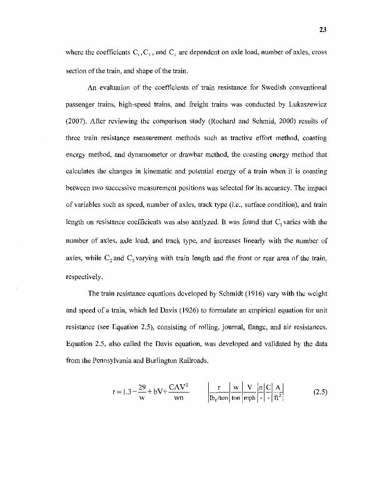
The train resistance equations developed by Schmidt (1916) vary with the weight
and speed of a train, which led Davis (1926) to formulate an empirical equation for unit
resistance (see Equation 2.5), consisting of rolling, journal, flange, and air resistances,
Equation 2.5, also called the Davis equation, was developed and validated by the data
from the Pennsylvania and Burlington Railroads.

24
where r is unit resistance in pounds per ton; w is weight per axle in tons; b is an
experimental coefficient based on flange friction, shock, sway, and concussion. C is the
drag coefficient based on the shape of the front end of the car or locomotive; and A is the
cross-sectional area in square feet of the car or locomotive. Later, the modified Davis
equation (see Equation 2.6) was developed in 1970 by Committee 16 of the American
Railway Engineering Association (AREA). Its intent was to recognize changes in
resistance factors, increased train operating speed, and improved track conditions over
the earlier days (AREA, 1981). The modified Davis equation is thus developed and
formulated as
where K, the air resistance coefficient, is 0.07 for cars, 0.0935 for containers, and 0.16 for
trailers on flatcars. Both the Davis and the modified Davis equations were derived for
calculating unit resistance of a train, which considered weight per axle, number of axles
per car, and the degree of aerodynamic and drag effects.
Hay (1982) discussed the effect of vertical and horizontal track alignments on
estimating train resistances. Grade resistance is proportional to the angle (in degree) of
the inclined track and can be directly derived from the relationship between train weight
and the track grade. It was found that the grade resistance was 20 lb/ton per track grade
(in percentage). On the other hand, the resistance associated with a horizontal track
curvature was determined by field tests and experiments (the Pennsylvania Railroad,
1907). It was found that the resistance due to horizontal curvature was 0.8 lb/ton per track
curvature (in degrees). While evaluating train resistances, Hay (1982) found that the total

25
resistance is the sum of all resistive forces acting on the train, which are measured in
pounds per ton. The evaluated resistive forces and their components are summarized in
Table 2.4.
Table 2.4 Characteristics of Train Resistances
ResistiveForces
ResistanceComponents Features
Load weightrelated
RollingResistance
• Results from friction between the wheel tread and thehead of the rail
• Function of the coefficient of rolling friction• Types of metal in wheel and rail• Condition of wheel and rail surfaces
TrackResistance
• Results from deflection and reverse bending of thetrack due to the loading and stiffness of the trackstructure
JournalResistance
• Results from the friction between the journals at theends of each axle and brasses
Velocityrelated
AirResistance
• Varies approximately with the square of the speed anddirectly as the cross-sectional are
• Air resistance =CAV2
o where C: experimental coefficiento A: cross-sectional area (ft2)o V: velocity (mph)
Curvaturerelated
CurveResistance
• Friction between the flanges and treads of the wheels• The head and gage corner of the rails due to track
curve
Graderelated
GradeResistance
• Major impact on the number of trains, locomotiveunits, and horse power to move given tonnage
Source: Hay (1982)
Bernsteen et al. (1983) studied the problem of train rolling resistance as an energy
consumption end use. Two types of freight train cars (e.g., 120-ton cars and 40-ton cars)
were tested to measure the rolling resistance and its effect on energy consumption for
various tracks classes [Track Classes 3, 4, 5, and 6 (a system of classification for track
quality has been developed by the FRA and each track class has its own speed limit as
shown in Table 2.5)]. It was found that the accuracy of the modified Davis equation

26
decreased when axle load is extremely low, which had an impact on rolling resistance. It
was also found that since the rolling resistance strongly depends on class of track, the
surface of track alignment should be improved to achieve better energy efficiency,
Table 2.5 Track Class and Train Speed Limit
Speed Limit (mph)TrackType
Freight Train PassengerTrain
Excepted' < 10 Not allowedClass 1 10 15Class 2 25 30Class 3 40 60Class 42 60 80Class 5 3 80 90Class 6 110Class 74 125Class 8 5 160Class 96 200
1. Only freight trains are allowed to operate on Excepted track and they may only run at speeds up to10 mph (16 km/h). Passenger trains of any type are prohibited.
2. Mainline track owned by major railroad company3. Burlington Northern Santa Fe (BNSF) railway & Amtrack's Southwest Chief4. Most of Amtrack's Northeast Corridor5. Portion of the Northeast Corridor6. Currently no Class 9 TrackSource: Federal Railroad Administration Track Safety Standards Compliance Manual (2007)
2.4 Train Control Regimes
Energy consumption and travel time on fully controlled systems are exclusively affected
by train control and less interfered by external factors such as traffic, signals, and
pedestrians (Vuchic, 1982). Therefore, a number of studies (Hopkins, 1978; Yasukawa,
1987; Howlett and Pudney, 1995; Duarte and Sotomayor, 1999) focused on optimal train
control for minimum energy consumption, In general, train control for most transit
operations represents a cycle of different motion regimes, including acceleration, cruising,
coasting, and braking. For analyzing station-to-station travel time and distance profile, it

27
is essential to comprehend the description of the motion regimes and their mathematical
expressions, which will be discussed in Chapter 3.
Four basic train controls and their motion regimes discussed by Vuchic (1982) are
shown in Figure 2.4:
Figure 2.4 Four cases of inter-station train control regimes.
• Control I: Acceleration, then braking must apply;
• Control II: Acceleration, cruising, then braking must apply;
• Control III: Acceleration, cruising, coasting, then braking must apply; and
• Control IV: Acceleration, coasting, then braking must apply.
Each case contains a set of motion regimes (e,g., acceleration, cruising, coasting, and
braking) affected by station spacing, acceleration/deceleration rates, and maximum
operating speed, denoted as Vm . Controls I and II are used to achieve the least travel time
for station spacing, denoted as S, is less and greater than the critical station spacing,

28
denoted as S e , respectively. In addition, Controls II, III, and IV are all used for S> S e . In
Control II, a train accelerates until VM is reached, and then VM is maintained until a brake
must be applied to stop at the next station. It is obvious that Control II operation drives
shorter travel time but consumes more energy, compared to those in Controls III and IV.
Control III operation is commonly used for reducing energy consumption, which consists
of an acceleration interval to reach VM , cruising at that speed, coasting, and then braking.
By using Control IV operation, the consumed energy can be further reduced, albeit the
longest travel time.
Hopkins et al. (1978) measured train energy consumption for various rail services
such as branch line freight, inter-city freight, high speed passenger, and commuter
considering train speed, size (weight and length), power to weight ratio, and track profile.
It was found that a continuously varying speed profile could consume an additional
energy of 5 - 15% than that of a constant speed profile (i.e., cruising), although both
yielded the same average speed, which indicated that a train operated with frequent
acceleration and braking consumes more energy.
Yasukawa et al. (1987) investigated several energy-efficient train controls for the
Tohoku Shinkansen electric motor trains by employing a simulation approach. Four
different train controls were simulated on the rail segment between Ohmiya and Oyama
stations. As illustrated in Figure 2.5, the proposed train controls used the same
acceleration rate until the train speed reaches VM , then the following motion alternatives
will take place:
• Control 1: cruising with VM , decreasing speed with automatic train control (ATC)
brake, cruising again, and then braking ;

29
• Control 2: coasting, decreasing speed with ATC brake, cruising, and then braking;
• Control 3: cruising, speed decreasing using ATC brake, coasting, and then
braking; and
• Control 4: coasting, speed decreasing using ATC brake, coasting again, and then
braking,
It was found that Control 4 is the most energy-efficient for which approximately 10%
energy can be saved, compared to other controls.
Figure 2.5 Train controls of the Tohoku Shinkansen.
Duarte and Sotomayor (1999) determined train speed trajectories with an optimal
control of a train in subway systems, The objective function of the study was minimizing
the total energy consumption for a round trip. Several constraints such as speed limit,
maximum slope of track alignment, maximum acceleration/deceleration rate, and
maximum electrical force were considered. The Gradient-Restoration method developed
by Miele et al. (1974) was employed to design an optimal train control used at a subway

30
system in Santiago, Brazil. An average of 18 % energy saving per train was achieved
after executing the optimal train speed profile.
Hiraguri et al. (2004) proposed a train control method based on the prediction of
train movement and data communication. The control method intended to avoid
unexpected train movement, such as an abrupt deceleration or stopping due to the delay
of the preceding train. The concept of the control method was to calculate the predicted
time when the preceding train leaves the station and transmit the predicted time to the
approaching train, and then the speed profile of the approaching train was controlled to
avoid an unexpected stopping. The proposed method was verified in computer simulation
and the performance of recovery from traffic disruption was evaluated. The simulation
results showed that the proposed method reduced stopping delay between stations and
related energy consumption.
Dongen and Schuit (1989) investigated several energy efficient driving strategies
of an electric railway system connecting Zandvoort-Maastricht and Heerlen in the
Netherlands. They analyzed energy savings, considering energy efficient acceleration,
optimized constant speed, and coasting. The energy saving test was conducted in co-
operation with the traffic center and train drivers were informed of the optimal control.
The test results of driving strategies consisting of optimized acceleration rate, constant
speed, and coasting revealed that approximately 25% of the energy consumption under
ideal train service circumstances (i.e., undisturbed condition) was saved, while 15% of
the energy under unexpected situations (i,e., temporary speed restriction, signal checking,
etc.) was saved.

31
2.5 Minimization of Energy Consumption for Train Operation
A number of studies related to minimizing train energy consumption have been
researched by using classical numerical optimization methods such as dynamic
programming (Franke et al., 2000; Albrecht, 2004) and the maximum principle (Horn,
1971; Golovitcher, 2001) as well as modern heuristic optimization algorithms such as the
Genetic Algorithm (GA) (Chang and Sim, 1997; Wong and Ho, 2003; Bocharnikov et al.,
2007), and fuzzy logic combined with GA (Hwang, 1998).
Previous studies on train energy consumption minimization used to over simplify
train movement (Horn, 1971) and ignored the effect of track alignment, which
considerably influences train resistances and tractive effort (Albrecht, 2004; Hwang,
1998).
Franke et al. (2000) used discrete dynamic programming to minimize train energy
consumption by considering the non-linear aspect of train control. Energy was set as a
dynamic state variable to minimize energy consumption on a level (without grade and
curvature) track alignment. An equation for train motion was formulated in the form of a
piecewise function, which was tested on the Zurich-Luzern line of the Swiss Federal
Railways (SBB) and achieved 10-30% reduction of traction energy.
Albrecht (2004) investigated the possibilities of train running time modification to
reduce power peaks and energy consumption under a given headway. The problem of
adjusting train running was regarded as a multi-level decision problem because it has to
be decided at each station and solved using dynamic programming. A case study has been
conducted for one line of the Berlin S-Bahn network consisting of a track of 18
kilometers (km) with 14 stations, Given that an optimal combination of headway and

32
synchronization time are known, it was sufficient to use a controller based on the
minimization of a single train's energy consumption using dynamic programming. The
optimized train running time could lead to energy savings of 4%.
Horn (1971) discussed that a number of studies on energy efficient train control
analytically approached a simplified linear train model by using the Maximum principle
in the late 1960s. Most optimal controls achieved by the Maximum principle were based
on the assumption that an inter-station train movement is composed of four motion
regimes: maximum acceleration, cruising, coasting, and maximum deceleration. The
application of optimal control was possible when this assumption was met.
Golovitcher (2001) developed an analytical method to achieve optimal train
control for minimum energy consumption in rail or other fixed path vehicles. To decrease
on-board computational time, he used a Hamiltonian formulation and the maximum
principle to determine the set of optimal controls, Based on the results obtained by
solving the Hamiltonian, a set of motion regimes (e.g,, full tracking, full braking,
coasting, cruising, partial tracking and partial braking) was established. The results of the
conjugate function of the Hamiltonian, traction effort equation, and braking power
equation set up criteria for using motion regimes, In a case study, the optimal control
could save 3% of the energy consumption.
Hwang (1998) developed a fuzzy control model which determines an economical
(i.e., the most energy efficient) train running profile considering the trade-off between
travel time and energy consumption, A speed triplet set (coasting speed, economical
speed, and maximum speed) was prepared through simulation runs and was optimized by
a proposed GA hybrid method (GA combined with a fuzzy model), but track alignments

33
were not considered. The studied GA hybrid method was used to a high-speed rail system
from Seoul to Busan in Korea. It was found that when the increase of travel time is less
than 7%, more than 5% of the energy consumption was saved.
, GA was used to search for the appropriate coasting control in a mass rapid transit
(MRT) system. Chang and Sim (1997) developed a dynamic train coasting regime
controller and a coasting control table by using GA to determine the timing for coasting
and to resume acceleration. Each coasting table was encoded into variable lengths of
chromosomes with each gene representing the relative position between stations where
coasting should be initiated or terminated. It was found that the use of GA to obtain
optimized coast control strategies is successful in improving energy consumption. Later,
a similar but enhanced study was conducted by Wong and Ho (2004). They used GA to
identify the best coasting locations, and the possible improvement on the fitness of genes
was investigated. Single and multiple coasting control with GA were developed and their
corresponding train movement was examined. Further, a Hierarchical Genetic Algorithm
(HGA) was adopted to identify the number of coasting locations required according to
the traffic conditions, and Minimum-Allele-Reserve-Keeper (MARK), a fast and
effective mutation scheme for GA, was used to a genetic operator to achieve fitter
solutions.
Bocharnikov et al. (2007) used GA to find an optimal coasting strategy combined
with varying acceleration and deceleration rates. They derived a fitness function
consisting of energy consumption and running time. Fuzzy sets were implemented and
optimal control sought which minimized energy consumption within the defined

34
timetable constraints. It was found that on a 8,53 km track, up to 31.27% of traction
energy was saved while travel time increased by 12.5%.
Kim and Chien (2010) developed an optimization model for rail transit to
minimize energy consumption used for an inter-station run. The model optimizes the
duration of train motion regimes used for train control by considering track geometry,
speed limit, and scheduled travel time using the Simulated Annealing algorithm (SA),
The model was used in a real case study of the Metro-North Commuter Railroad. The
most energy efficient train control, or called "golden run", associated with speed limits,
track geometry, and schedule adherence was identified. It was found that the optimal
train control saved 30.4 % of the energy consumption in a commuter rail system
compared with flat-out run, while travel time increased by 7 %.
Energy minimization for rail public transit systems was discussed by Danziger
(1975) from the viewpoint of an integrated systems approach. The approach considered
the interaction of all the major subsystems of a rapid transit system rather than each
subsystem independently. Some of the major subsystems examined included vehicles and
their major propulsion, braking and auxiliary systems, train operations, environmental
control facilities, and civil and structural facilities. The major factors that may
significantly affect an overall energy evaluation were identified, and the ways in which
each of these factors can be controlled to affect overall maximum efficiency of energy
use were discussed. Energy evaluation techniques include a new strain performance
simulation computer program developed by Parsons, Brinckerhoff, Quade and Douglas,
Inc., as part of a 4-year subway environmental research project. It was found that the
procedures for evaluation on a total system-wide basis are applicable for any rail transit

35
system and can be used to extend or modify existing rail transit systems and the design of
new ones.
2.6 Optimization Algorithms and Heuristic Methods
The studied optimal train control problem is a large combinatorial optimization problem
where the solution space consists of combinations of multiple decision variables,
including motion regimes, locations of motion regime changes, and the acceleration rate.
Thus, a robust searching algorithm, such as Simulated Annealing and other intelligent
optimization techniques, is desired to find a near optimum solution efficiently in the
enormous solution space. Several optimization techniques, such as Simulated Annealing
(SA), Tabu Search (TS), and Genetic Algorithm (GA) are suitable to solve a
combinatorial problem, and are discussed below,
The simulated annealing (SA) algorithm derived from statistical mechanics was
developed by Kirkpatrick et al. (1983) based on the strong analogy between the physical
annealing process of solids and the problem solving of large combinatorial optimization
problems. The states of solid represent the feasible solutions of optimization problems, in
which the energy associated with each state corresponds to the value of the objective
function of each feasible solution. Accordingly, the minimum energy of a crystal state
corresponds to the optimal solution while rapid quenching can be considered as a local
optimization, A standard simulated annealing algorithm includes four portions (i.e.,
solution representation, objective function, generation mechanism of neighbor solutions
and has been cooling schedule). SA has been proven effective for fine-tuning a local
optimal search, and utilized to solve many optimization problems in transportation related
fields, such as transit network optimization (Zhao and Zeng, 2006), robust estimation

36
(Baselga, 2007), vehicle routing problem (Ting and Chen, 2007), road network design
(Kim and Schonfeld, 2008). However, a good initial solution and cooling schedule are
very critical in finding the optimal solution.
Busetti (2003) presented an overview of SA by discussing and comparing its
features with other optimization methods. The strengths of SA identified in his paper are
as follows:
• SA can handle highly non-linear models, chaotic and noisy data, and many
constraints.
• SA is flexible and able to find global optimality.
• SA is versatile and does not rely on any restrictive properties of the model.
• SA can be easily tuned, For any reasonably difficult non-linear or stochastic
system, a given optimization algorithm can be tuned to enhance its performance
and since it takes time and effort to become familiar with a given code, the ability
to tune a given algorithm for use in more than one problem should be considered
an important feature of an algorithm.
He also made a direct comparison between Adaptive Simulated Annealing (ASA) and
GA, using a test suite already adapted and adopted for GA. The result showed that in
each case, ASA outperformed the GA problem. He mentioned that GA is a class of
algorithms that are interesting in their own right; GA was not originally developed as an
optimization algorithm, and basic GA does not offer any statistical guarantee of global
convergence to an optimal point.
Zhao and Zeng (2006) presented a stochastic methodology for transit route
network (TRN) optimization. Their study goal was to provide an effective computation

37
tool for the optimization of a large-scale transit network to minimize transfers with
reasonable route directness while maximizing service coverage. The methodology
includes the representation of a transit route network solution search spaces,
representation of the transit route and network constraints, and a stochastic search scheme
based on an integrated SA and GA search method. The feasibility of the proposed method
has been tested through previously published results and a practical TRN optimization
problem of a realistic size, Numerical results showed that the methodology was capable
of tackling large-scale transit network design optimization problems.
Baselga (2007) proposed a methodology for robust estimation that has proven to
be a valuable approach to adjust surveying network when there are systematic or gross
errors in the observations or systematic errors in the functional model. He computed
robust estimation with SA and an Iteratively Reweighed Least-Squares (IRLS) process,
and compared the results of two methods. In his study, he mentioned that SA is one of the
most suitable heuristic methods for large-scale optimization problems, especially when
there is a global optimum, which is to be determined among many other local optima.
Ting and Chen (2007) developed a methodology to find the optimal solution of a
vehicle routing problem (VRP) which is an important management problem in the field
of physical distribution and logistics. The study proposed a multiple ant colony system
(MACS) to solve the multi-depot vehicle routing problem with time windows
(MDVRPTW), Moreover, two hybrid algorithms, which combine the strengths of the
MACS and the SA, were developed to improve the solution quality. The numerical
analysis demonstrated that the combination of MACS and SA can improve the solution
quality significantly.

38
Kim and Schonfeld (2008) extended the network design problem (NDP) to the
proposed road space allocation problem (RSAP), which finds the optimal lane
configuration on each link in a road network that minimizes total system cost. The RSAP
was formulated as a bi-level programming problem with an upper-level problem that
optimally allocates road space and a lower-level problem that evaluates travelers' mode
and route choices in response to each alternative. The demand model employs a multi-
class, multi-modal network equilibrium model to efficiently evaluate road space
allocation alternatives. A heuristic based on simulated annealing was presented to solve
the combinatorial optimization problem. It was found that when toll lanes are provided in
the network, in most cases, lower-income users have the longer average travel time than
higher-income users. With a lower allowable equity measure, a more equitable solution
was reached.
The literature review revealed that existing algorithms have different strengths in
solving particular optimization problems. For example, GA was found to outperform SA
and TS in solving traveling salesman problems (Pham and Karaboga, 2000). However, in
solving large-scale machine-grouping problems, Zolfaghari and Liang (2002) indicated
that SA outperforms both GA and TS, and GA is slightly better than TS,
2.7 Summary
Energy consumption is deemed to be a very important indicator for sustainable train
operation due to increased energy usage and cost. A number of studies have been
conducted to minimize energy consumption for train operations, but some of them
required the purchase of new equipment (e.g., kinetic energy storage system, variable
voltage variable frequency (VVVF) inverter, gate turn off (GTO) thyristor, etc.) that are

39
quite expensive. Therefore, implementing optimal train control subject to existing track
alignment and regulated speed setting may bring a significant benefit in comparison with
alternatives using costly technologies. Most of the previous studies shown in Table 2,6
have been focusing on developing optimal train control models to reduce energy
consumption, but those either disregarded the joint effect of varying vertical alignment
and horizontal curvature on TE and resistance or neglected the restriction of travel time
for schedule adherence. Instead, most of the train control studies were focusing on the
effect of train speed control or coasting regime on energy consumption and travel time.
This research develops methodologies that optimize train control by considering various
aspects (e.g., track alignment, maximum operating speed, schedule adherence, etc.) of
train operations.

40
Table 2.6 Minimum Energy Consumption for Train Operation Studies
Authors(Year) Methodology Limitation
Horn(1971)
•
•
Train control modelassumed linearOptimized using MaximumPrinciple
• Over simplified trainmovement
Chang and Sim(1997)
• Developed dynamiccoasting regime controllerby applying GA
• Proposed method wasdemonstrated for inter-stationtrain movement
Hwang(1998)
• DevelOped most energyefficient train runningprofile using a fuzzy controlmodel
• Effect of track alignment wasnot considered
Franke et al.(2000)
• Employed discrete dynamicprogramming to minimizetrain energy consumption
• Studied on only levelalignment
Golovitcher(2001)
• Developed analyticalmethod for optimal traincontrol by using maximumprinciple
• Only four sets of traincontrol are considered
Albrecht(2004)
• Adjusted train running timeusing dynamicprogramming
• Effect of track alignment wasnot considered
Wong and Ho(2004)
•
•
Determined best coastinglocations with GAIdentified the number ofcoasting using MARK
• Proposed method is notapplicable for a multipleinter-station run
Bocharnikov etal, (2007)
• Investigated an optimalcoasting strategy using GA
• Proposed method isappropriate only for inter-station train movement

CHAPTER 3
DEVELOPMENT OF TRAIN PERFORMANCE SIMULATION (TPS) MODEL
A time-driven TPS model which consists of three key modules: Train Traction Module
(TTM), Track Alignment Module (TAM), and Train Control Module (TCM), is
developed to simulate passenger train operations, which can be used to evaluate various
performance indicators, including travel time and energy consumption for any train
control and track alignment. Dynamic information, such as the TE, resistances, the rate of
acceleration/deceleration, and speed, will be generated corresponding to the location of a
train and the geometry of the track alignment. The development of each module is
discussed below.
3.1 Train Traction Module (TTM)
The responsibility of the train traction module (TTM) is to compute the TE needed to
move a train along a rail line, considering the speed, the rate of acceleration (or
deceleration), and the location of the train at any point in time. TTM calculates the TE
based on projected resistances so that the rates of acceleration/deceleration and the target
speed for the next interval operation can be obtained. The input parameters of TTM
include static information (e.g., locomotive power, number of cars per train, number of
axles per car, train weight, cross-section area), dynamic information (e.g., train location,
travel time, speed, rates of acceleration/deceleration), track alignment condition (e,g.,
convex, concave, level), and operational constraints (e.g., speed limit, station spacing,
and train schedule, etc.). An iterative computation process is performed based on a user-
41

42
specified time interval (e.g., 1 second), in which the needed TE to move the train to the
desired location over time can be determined.
The calculated TE with TTM can be used with different types of locomotives (e.g.,
diesel-electric and electric motors) for estimating consumed energy by justifying the ratio
of energy consumption per unit of TE. Note that the function of TE is calculated based on
the effective power to move tonnage up on the track alignment (e.g., level, convex, and
concave). The developed TTM computes TE and resistances of cars and locomotives of
the train by considering the train as a string of masses interconnected by springs and
damping as shown in Figure 3.1,
Figure 3.1 Longitudinal train forces on a cOntinuously varying track.
The net force to move each car of the train is equivalent to the differences
between TE, denoted as F, the sum of resistances (e.g., bearing, rolling, air, and grade
resistance), denoted as R, coupler forces determined by a damper constant (d) and spring
constant (k). Considering that locomotives of a train can be placed in any position, the
equation of motion for the car in a train, at time t , can be determined by Equation 3.1
discussed by Cole (1998).

43
where m, is car mass, a it is acceleration of the i th car at time t, d, is damping constant, k,
is spring constant, li t, is speed of the i th car at time t, x: is longitudinal position of the i th
car at time t,
To avoid slippage of the wheel on the track, the maximum TE at time t for the
i th car, denoted as Ftmax(i) , is the minimum value of available propulsive force, denoted as
F t and adhesive force, denoted as Fta(i). Thus,p(1)
As indicated in Eq. 3.2, 4 (1) represents a needed force for the wheel to overcome
the resistance is the product of locomotive's horse power for the i th car, denoted as Pit ,
and energy transmission efficiency, denoted as r1, divided by speed of the i th car, denoted
as Vti , at time t. Thus,
where 375 is a parameter to convert the unit rate of work in foot-pounds/second into
mile-pounds/hour. Note that Equation 3.3 is derived based on a function discussed by
Hay (1982) in which the transmission efficiency (77) is a coefficient of energy loss

44
between the engine and the wheels. 77 varies with the type of gears and is usually
between 0.78 and 0.85, depending on train speed and track condition.
On the other hand, F; ( represents a friction force caused by the contact between
the wheel of the i th car and track surface and is dependent on the car weight, denoted
as W, , and adhesive coefficient, denoted as pit . The determination of is based on the
train speed shown in Figure 3.2 (Vuchic, 2007), which ranges between 0.28 and 0,38 for
a speed of 10 kilometers per hour (kph) and between 0.17 and 0.28 for a speed of 80
kilometers per hour (kph) under dry rail and wheel conditions. In the developed TPS,
is assumed linearly decreasing as the train speed increases from 0 to 80 kph. Thus,
Note that g was found non-linearly decreasing with an increasing V,' (Candee, 1940),
which can be adapted by the developed TPS.
Figure 3.2 Adhesion coefficient vs. speed under different rail and wheel conditions.

45
The kinematics of the i th car movement at time t inclined at an angle B it to the
horizontal are determined by a couple of force components including TE, resistance and
train weight, denoted as Fit , Rti, and W, , respectively (See Figure 3.1). Therefore, the
adhesive force Fta( ,) for steel wheels on the rail, generated by the car weight component
perpendicular to the surface of the track, can be estimated by Equation 3.5 as
The resistances of a train consists of three principal components, including
bearing resistance, rolling resistance, and aerodynamic resistance, The first two
resistances purely depend upon the speed and weight of the train, while the third one is
affected by the direction and speed of wind as well as the size, shape, and speed of the
train. The unit resistance of the car at time t, denoted as R tu(i) , can be obtained by the
following modified Davis equation as:
where w i represents car weight per axle; G; represents grade percentage; ID; represents
track curvature; and K, and n, are the aerodynamic coefficient and the number of axles
per car, respectively. Note that Vrt represents relative train speed based on the direction of
wind speed ( ) as shown in Figure 3.1. Thus,

46
where θtwd(i) is the angle between the directions of wind and car movement.
The resistance of the i th car at time t, denoted as Rt i , is the product of unit
resistance (K ( , ) ), car weight per axle (w i ), number of axles per car (n, ), and number of
cars per train (N). Thus,
The net force to move a car in a train was formulated in Equation 3.1, and is equal
to the TE minus the resistance combined with forces resulting from damping and springs.
Note that the net force of the i th car at time t divided by the train mass represents
acceleration, denoted as at i . Thus,
where W, represents the i th car weight, while p and g are the coefficients of rotating mass
and gravitational acceleration, respectively. The process of calculating train deceleration
is similar to that for calculating acceleration, which is determined by actual braking force,
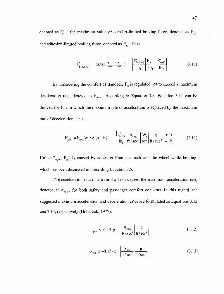
47
denoted as Ftb(i) , the maximum value of comfort-limited braking force, denoted as Fb„
and adhesion-limited braking force, denoted as F ba . Thus,
By considering the comfort of standees, F bc is regulated not to exceed a maximum
deceleration rate, denoted as b.. According to Equation 3.8, Equation 3.11 can be
derived for Fbc , in which the maximum rate of acceleration is replaced by the maximum
rate of deceleration. Thus,
Unlike Fbc(i) Fba(i) is caused by adhesion from the track and the wheel while braking,
which has been discussed in presenting Equation 3.5.
The acceleration rate of a train shall not exceed the maximum acceleration rate,
denoted as a max , for both safety and passenger comfort concerns, In this regard, the
suggested maximum acceleration and deceleration rates are formulated as Equations 3.12
and 3.13, respectively (Hoberock, 1977):

48
Since the TE in the proposed TPS model is calculated based on a user specified
time interval, denoted as At , a train car's speed and travel distance can be estimated
based on the rate of acceleration or deceleration determined in every interval, The
increment of train speed, denoted as Δv t , from t to t+1 is the product of the acceleration
rate and the duration of the time interval ( At in Equation 3.14). The associated travel
distance of the i t" car, denoted as Ax: , is formulated as Equation 3.15:
To move the i t" car in a train at speed Vit , an equation used to calculate the engine power
consumed at t, called Pit , is derived based on a function discussed by Hay (1982), Thus,
The energy consumption rate e ti required to either propel or brake during At can
be derived as

49
Note that the unit engine power (hp) is equal to 0.7457 kilowatts (kW), and the time
interval (sec) divided by 3,600 is converted to an hourly base. The total energy
consumption, denoted as E, over the route segment can be obtained by integrating the
power required over time. Thus,
where J is the number of time steps needed for traveling from one station to another.
3.2 Track Alignment Module (TAM)
A vertical track profile is a combination of segments with different grade percentages and
transition sections, which need a sag curve and/or a crest curve for smooth connection,
Transition rates in grade in 100 ft, denoted as y, can be estimated by Equation 3.19, and
the recommended transition rates by AREA are 0,05 and 0,1 for sag and crest curves,
respectively (Hay, 1982),
where G 1 and G2 are two adjacent track grades, and L is the horizontal track length.
TAM converts a given vertical track profile into a series of track grades delivered
to TTM for calculating train resistances and the TE, which exchanges data (e.g., track
grade and train position) in every simulation time step. TAM also provides information
(maximum operating speed, denoted as VM ) to the Train Control Module (TCM) so that a
proper track alignment can be referred to determine the regime of motion (e,g,,

50
acceleration, cruising, coasting, and deceleration, etc.). A step procedure summarized
below discusses the interaction between TAM and other modules (e.g., TTM and TCM).
• Step 1: Identify the number of inflection points of track alignment and divide the
station spacing (S) into a number of segments based on the inflection points.
where q is the total number of segments and j is the segment number in vertical
alignment
• Step 2: Develop equations for representing vertical track alignment for segment I
identified in Step 1, denoted as yj(xt), where x t is the traveled distance at time t
(ft).
• Step 3: Differentiate y j (x t ) over distance to obtain track grade G tj at segment j.
• Step 4: Input Gtij to TTM and y j (x t ) to TCM for calculating train resistance and
TE and determining the regimes of motion.
• Step 5: Input Gtj and data to TTM in every time interval and receive travel
distance (Δxt ) data from TIM. Note that Δx t = xt - xt-1,

51
3.3 Train Control Module (TCM)
The responsibility of the Train Control Module (TCM) is to determine the appropriate
motion regime based on TE and track alignment information computed by TTM and
TAM, TCM will first generate feasible plans formed by different motion regimes, As
shown in Figure 4, a general train control, denoted as TC, consisting of accelerating (M a ),
first coasting ( Mc1 ), cruising ( M, ), second coasting ( ), and braking ( M b ) is
developed for discussing feasible plans. Note that the relationship between speed and
time is not necessarily linear.
Figure 3.3 Configuration of a speed profile for a general train control on SVA.
While M a and M b are always essential for accelerating and decelerating a train
departing from and arriving at a station, three other motion regimes ( , M, , and M e, )

52
are optional and can be integrated with M a and M b . For instance, if the durations for the
1 st and 2nd coasting regimes are equal to zero ( tc1 = tc2 = 0) the resulting train control only
consists of accelerating, cruising, and braking regimes. However, if the durations for the
1 st coasting and cruising are equal to zero (tc1 = tV = 0), the resulting train control consists
of accelerating, coasting, and braking, It is considered that coasting is usually a beneficial
motion regime for rail operators because it may save considerable energy; however a
longer travel time between stations should be expected.
Considering various track alignments (level, convex, and concave) and applicable
motion regimes, the feasible train controls for each alignment are summarized in Table
3.1. It is worth noting that the applied train controls in the developed TPS are not
necessarily limited to the train controls below.
• Train Control 1 (TC1): Considering cruising regime ( M y ) associated with M a
and Mb
• Train Control 2 (TC2): Considering cruising and both coasting regimes (e.g.,
Mc1 and/or Mc2 ) associated with M a and Mb
• Train Control 3 (TC3): Considering coasting regimes (e,g,, M c1 and/or Mc2 )
associated with M a and Mb

53
Table 3.1 Feasible Train Controls
TrackAlignment
Train Controls and Motion Regimes
(1) TCL1 =Ma +My ±Mb
Level (2) TCL2 = Ma + My + Mc2 + Mb
(3) TCL3 = Ma + Mc2 + Mb
(1) TCU1 = Ma + My + Mb
Convex (2) TCU2 = Ma + Mc + My + Mc2 + Mb
(3) TCU3 = Ma + Mc1 + Mc2 + Mb
(1) TCD1 = M a + My + Mb
Concave (2) TC 2D = M a + M c1 + M, + Mb
(3) TC 3D = M a +M c +Mb
While a general train control consists of the five motion regimes
as M a , Mc1, MV, Mc2, and M b , the station-to-station travel time denoted as T (excluding
dwell time at stations) can be formulated as
where t a, tc1, tV, t C, and tbrepresent travel times (sec) for acceleration, the 1stcoasting,
cruising, the 2 nd coasting, and braking, respectively, which can be calculated with
Equations 3.23 to 3.27 formulated as
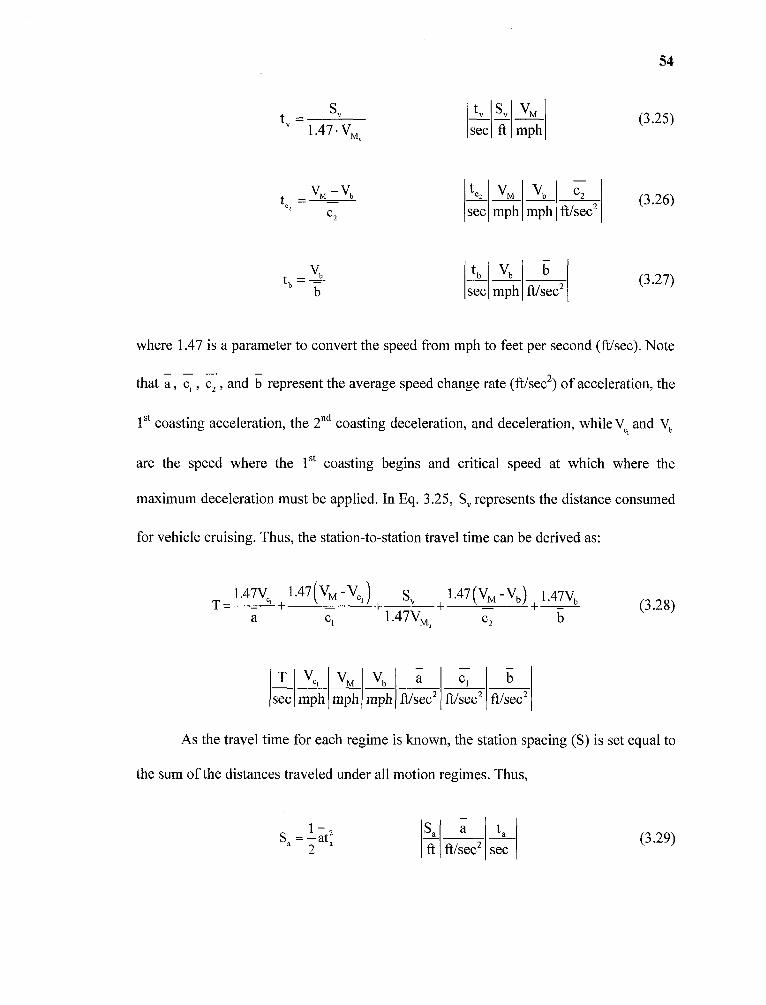
54
where 1.47 is a parameter to convert the speed from mph to feet per second (ft/sec). Note
that a, c, , c, , and b represent the average speed change rate (ft/sec2) of acceleration, the
1 st coasting acceleration, the 2nd coasting deceleration, and deceleration, while V„ and Vb
are the speed where the 1 5t coasting begins and critical speed at which where the
maximum deceleration must be applied, In Eq, 3,25, S, represents the distance consumed
for vehicle cruising. Thus, the station-to-station travel time can be derived as:
As the travel time for each regime is known, the station spacing (S) is set equal to
the sum of the distances traveled under all motion regimes. Thus,

55
where Sa, S c1 , Sc2 , and Sb represent the travel distances (ft) for acceleration, the 1 st
coasting, the 2nd coasting, and deceleration, respectively, Thus, the station spacing
denoted as S can be derived as:
To derive the cruising time (t `, ), the difference of station spacing and the
distances traveled during the regimes of acceleration, the 1 st coasting, the 2 nd coasting,
deceleration is divided by VMi .

With Equations 3.34 and 3.35, the cruising time can be defined as:
56
The three modules in the proposed TPS model simulate train movement every
second on an iterative basis. A complete cycle of the proposed TPS calculation in each
time interval is shown in Figure 3.4, and the step procedure is discussed below.
• Step 1. Start the simulation and feed input data (e.g., motor power, car weight per
axle, number of car, number off axle) to TTM and TAM.
• Step 2. Calculate TE, train resistances, and speed at time t with TTM.
• Step 3. Determine train control (e.g., TC1 TC 2 , and TC 3 ) and check if the Pt
coasting ( M c ) can be applied at time t (e.g., V t ≥ Vc1 ) with TCM.
• Step 4. If V Vu in TTM, go to Step 6. Otherwise, calculate traveled distance
and consumed energy for acceleration, and update simulation clock (i.e., t = t+1),
then go to Step 2.
• Step 5. Determine motion regime (e.g., M y , M c2 , and M y + Mc2) with TCM.
• Step 6. If the remaining distance (RD) is less than the stopping distance (SD),
decelerate the train, calculate consumed braking energy in TTM, update the
simulation clock, and then go to Step 7, Otherwise, go to Step 2,

57
• Step 7. If the train arrives at the station, end simulation clock, report consumed
travel time and energy, and terminate the simulation, Otherwise, go to Step 6.

Figure 3.4 Flow chart of the train performance simulation model.
58

CHAPTER 4
METHODOLOGY
The objective function (i,e,, total energy consumption) for the four cases discussed in
Chapter 1 is formulated in this chapter. The objective total energy consumption function
is affected by various factors such as train control between a pair of stations, the topology
of track alignment and schedule adherence. A set of system assumptions is made to
formulate the research problem for each case and the associated constraints, which are
discussed in Sections 4.1 through 4.4 for Cases I through IV, respectively, The developed
models are based on the different vertical track alignments such as single vertical
alignment (SVA) and mixed vertical alignment (MVA) associated with fixed and variable
maximum operating speed (MOS) over the route. The optimal solutions for the cases are
obtained considering the appropriate train control as well as the scheduled travel time.
4.1 Model I - SVA and Constant MOS (Case I)
The model formulated in Case I is designed to optimize train control over a SVA
combined with a constant MOS. To formulate the model, system assumptions on the
geometry of track (i,e., vertical track alignment), train control (i.e., applied motion
regime), and train characteristics (e.g., tractive effort (TE), resistance, acceleration/
deceleration rate, train movement calculation, etc,) are made,
59

60
4.1.1 Assumptions
To formulate the research problem discussed in Case I, a list of assumptions is made and
discussed below:
1. A generalized vertical rail alignment, which may be symmetric and parabolic,connecting stations A and B as shown in Figure 4.1 can be classified into threetypes (level, convex, and concave) of track alignments. It is worth noting that the"level" alignment indicates a tangent curve with zero grade. Note that the terms"convex" and "concave" alignments used in this study consist of "crest" and"sag" curves, respectively, with both ascending and descending grades, To obtaina continuous vertical track profile and associated track gradient, a general trackalignment which is a function of station spacing (S), inflection points (I n), andvertical depth/ height (ö) at halfway between two stations is assumed as:
where y1(xt), y 2 (x t ), and y3 (x t ) represent elevations with respect to x t in feet
on different segments, while G: is the gradient at xt in percent, and Δ 1 , A 2 , and
Δ 3 are 1/6, 2/3, and 1/6 of S, respectively, as shown in Figure 4.1.
Figure 4.1 Single vertical alignment between stations A and B.

61
2. The train will use the maximum TE from stand still until it reaches the maximumoperating speed ( VM ) and the maximum deceleration rate will be used when the
remaining distance (RD) is equal to or less than the stopping distance (SD),
3. Four motion regimes are considered, including accelerating, cruising, coasting,and braking. Note that cruising is applied when there is a need.
4. The train movement and its related forces are treated as a string mass on a route.Accordingly, the forces related to train movement, such as TE and resistance, arecomputed individually for all cars and locomotives.
4.1.2 Model Formulation
The motion of a train can be determined by the difference between the total TE (E)) and
resistance (R Tt ), which are directly affected by the train speed and vertical track grade.
Thus, F'.. and RTt at time t are functions of speed and vertical track grade represented by
f, and f2 respectively , which can be re-formulated as:
where J is the total number of time steps needed for traveling between two stations.
With Equations 4.4 and 4.5, the acceleration rate at time t, denoted as at, can be
determined by
where p is the coefficient of rotating mass and m is the train mass.

62
The consumed engine power Pt (also in Equation 3.16) for speed V' at time step
t can be formulated as:
The energy consumption e t is equal to the product of power used from t to t+ Δt
and the duration of the simulation time step, and can be expressed as:
Note that the unit engine power is equal to 0.7457 kilowatts, and the time interval divided
by 3,600 is converted to an hourly base. Accordingly, the total consumed energy, denoted
as E, for a train movement between stations A and B is the sum of energy used in all time
steps:
As shown in Equations 4,4 through 4.9, the total energy consumption is directly
affected by train speed and vertical track grade, While the track grade is known, the
desired train speed can be reached by determining an acceleration rate,
4.1.3 Constraints
The constraints considered in this study include the maximum operating speed, allowable
travel time and maximum acceleration/deceleration rates while optimizing train control,
The first constraint ensures that the train speed at time t does not exceed the MOS based

63
on track alignment and operations. Considering a constant maximum operating speed
(e.g,, fixed MOS) assumed in Case I, Equation 4.10 must hold.
The second constraint establishes that the range of travel time under optimal train
control must be less than or equal to the maximum allowable travel time (e.g,, travel time
for a train from the upstream station to the downstream station before the scheduled
arrival time). The travel time between stations, denoted as T , is ruled by the maximum
allowable travel time, denoted as TM .
Note that when a train is already behind schedule, it will use the maximum TE to
overtake the scheduled travel time. Three motion regimes including accelerating, cruising,
and braking will be used.
The third constraint certifies that the acceleration rate at any time t does not
exceed the passenger comfort limit. The maximum acceleration rate, denoted as amax,
used in the previous studies (Hoberock, 1977; Martinez et al., 2004; Koo et al., 2006) is
0.15. g (i,e., 4.8 ft/sec 2). Thus,

4.1.4 Optimization Model
Based on the discussion in Sections 4.1.1 through 4,1.3, the model developed for the
research problem in Case I of minimizing total energy consumption considering the effect
of train power, track alignment, speed regulation, and schedule adherence is formulated
below:
4.2 Model II - SVA and Variable MOS (Case II)
Model II is enhanced from Model I, and minimizes energy consumption considering
single vertical alignment (SVA) with a variable MOS. The model assumptions,
constraints, and optimization problem for Case II are discussed next.
4.2.1 Assumptions
The assumptions made for formulating the model are the following;
1. The general condition of a single vertical track alignment discussed in Section4.1.1 is also considered in Case II.
2. The assumption discussed in Section 4.1.1 is also used here. The train usesmaximum TE for the initial acceleration until it reaches VM and maximumdeceleration for the final braking to stop at the downstream station,

65
3. Four motion regimes are considered, including accelerating, cruising, coasting,and braking. Note that the cruising regime is used when there is a need.
4. The movement of the train and its related forces are treated as a string mass on aroute. Thus, the forces related to train movement, such as TE and resistance, arecomputed separately for all cars and locomotives.
The functions for computing train movement and estimating total energy
consumption (E) are the same as those used in Case I. The total travel time and
acceleration rate constraints considered in Case I can be used in Case II. However,
multiple maximum operating speed constraints (i.e,, variable MOS) are used in Case II as
shown in Figure 4.2, and train speed never exceeds the variable MOS. Thus,
where u is the index of maximum operating speed used.
Figure 4.2 Feasible variable MOS profile on SVA in Case II.

66
4.2.2 Optimization Model
Based on the previous discussion, the studied train control optimization model that
minimizes total energy consumption under SVA subject to the variable MOS, the
maximum total travel time, and the maximum acceleration rate is the same as discussed
in Case I and formulated as follows:
4.3 Model III - MVA and Constant MOS (Case III)
The model developed in Case III is enhanced from Model I developed in Case I, and
minimizes energy consumption for a train running on a mixed vertical alignment (MVA)
with a constant MOS. Other than track alignment, all assumptions made for Case I are
used in Case III.

67
4.3.1 Assumptions
Model III is developed to optimize train control over a mixed vertical curve with constant
MOS. The following assumptions are made:
1, A mixed vertical alignment that connects stations A and B is considered in CaseIII, The alignment may be asymmetric, and may consist of seven types of trackcurves, including ascending crest, descending crest, ascending sag, descendingsag, ascending tangent, descending tangent, and flat tangent as shown in Figure4.3. A continuous vertical track profile and associated track gradient may beachieved by formulating a general track alignment which is a function ofhorizontal track segment distance and vertical depth/height at two consecutiveinflection points (In):

68
where y 1 (x t ) through y 7 (x t ) represent elevations with respect to x t in feet on
different segments, while Gtj is the gradient at x t in percent for Δ 1through Δ7.
Note that the MVA used for Case III is not necessarily the same as that in Figure4,3.
Figure 4.3 Feasible mixed vertical alignment between stations A and B,
2. As discussed in Section 4.1.1, a train uses the maximum TE for the initialacceleration until it reaches VM and then maximum deceleration is used for thefinal braking to stop at the downstream station.
3. Four motion regimes are considered, including accelerating, cruising, coasting,and braking. Note that cruising is used when there is a need.
4. The train movement and its related forces are treated as a string mass on a route.Thus, the forces related to train movement, such as TE and resistance, arecomputed separately for all cars and locomotives.
The functions for estimating train movement and energy consumption (E) are the
same as those developed for Cases I and II. The train speed, total travel time, and
acceleration rate constraints considered in Case III are the same as those used in Case I.

69
4.3.2 Optimization Model
Based on the discussion in Section 4.3.1, the studied train control optimization problem
that minimized total energy consumption under MVA combined with the constant MOS
is formulated as follows:
4.4 MVA and Variable MOS (Case IV)
The model in Case IV considers mixed vertical alignment, which is used in Case III,
combined with variable MOS to optimize train control for minimum train energy
consumption. The assumptions, constraints, and optimization problem for Case IV are
discussed next.
4.4.1 Assumptions
The Case IV model considers mixed vertical alignments with a variable maximum
operating speed. The assumptions made for formulating the model are as follows:
1. The track alignment considered in Case IV is the same as discussed in Section4.3.1.

70
2. The train acceleration for the initial acceleration and the final braking is the sameas discussed in Section 4.1.1,
3. The motion regimes are the same as discussed in Section 4,1.1, includingaccelerating, cruising, coasting, and braking. Note that cruising is used when thereis a need.
4. The train movement and its related forces are treated as a string mass on a route.
The functions for train motion and total energy consumption (E) are the same as
those used in Cases I, II, and III. The constraints for the maximum operating speed, total
travel time, and the maximum acceleration rate in Case IV are same as those in Case II,
Thus, multiple MOS constraints (e.g., variable MOS) as shown in Figure 4.4 are used in
Case IV. Note that the used MOS and MVA for Case IV are not necessarily the same as
those shown in Figure 4.4.
Figure 4.4 Feasible variable MOS profile under MVA in Case IV.

71
4.4.2 Optimization Model
Based on the discussion from Section 4.4.1, the studied train control optimization model
that minimizes total energy consumption under MVA subject to the variable maximum
operating speed, the maximum total travel time, and the maximum acceleration rate is
formulated as follows:
4.5 Summary
In this chapter, the objective total energy consumption functions and sets of constraints
for Case I through IV were formulated. The developed optimization models are based on
the assumptions and constraints, which are determined based on the type of track
alignments and the number of maximum operating speed. The decision variables used in
each model are motion regimes (e.g., acceleration, cruising, coasting, and braking). While
considering the given track alignment and speed constraint in Cases I through IV, the
optimization model can be solved by using the SA algorithm to minimize total energy
consumption.
CHAPTER 5
SOLUTION METHODS
As discussed previously in Chapter 4, the objective of this study is to develop models to
optimize train control that minimizes energy consumption under Cases I through IV. The
decision variables to be optimized include the timings, durations, and locations of the
motion regimes and the rates of acceleration and deceleration.
The train control problem discussed in this study is a combinatorial optimization
problem. The timings and locations of motion regimes and acceleration (or deceleration)
increase as the complexity of track alignment, the number of feasible motion regimes and
speed constraints increase. A meta-heuristic algorithm, called Simulated Annealing
Algorithm (SA), is developed and used to search for the optimal solution. Furthermore, a
number of train controls are developed and discussed by considering train speed and
schedule adherence constraints in Cases I through IV.
5.1 SVA with Constant MOS (Case I)
5.1.1 Train Control
A set of train control profiles consisting of combinations of motion regimes must be
established and used to regulate train movement. As discussed in Section 4.1, a single
vertical alignment (SVA) associated with a constant maximum operating speed (MOS) is
considered in Case I. With these conditions, a general 4-regime train control illustrated in
Figure 5,1 is used to minimize energy consumption with SA, The used train control
72

73
profile consists of four motion regimes, including acceleration, cruising, coasting, and
braking.
Figure 5.1 Train control with four motion regimes.

74
The energy consumed in Case I is essentially affected by the timings and durations of
individual motion regimes, which will be optimized through the minimization of energy
consumption
In general, if the schedule allows and/or a sufficient momentum exists, a coasting
regime may be triggered before a train reaches the MOS (see Figure 5.1). As the speed
for coasting (or cruising), denoted as Vo is found, the timing and position to hit V'O is a
reference to change the motion regime from acceleration to coasting (or cruising). Unless
the coasting regime is commenced with speed of K, a cruising regime is used to
maintain the speed K. In case a cruising speed K is used, the timing and location for
the coasting must be identified. As shown in Figure 5.1(b), an optimal V'O is found
between VM, and Vmin. Note that the Vmin can be determined with the given maximum
allowable travel time. In addition, a feasible location for coasting, denoted as Cp , may be
found between the times when the regime of acceleration ends and deceleration starts.
The feasible ranges for K and C, are affected by various factors, including station
spacing, track alignment, scheduled travel time, acceleration (or deceleration) rate, etc.
Note that, if a coasting regime is triggered too early, re-acceleration is needed and more
energy will be consumed.
5.1.2 SA for Case I
The energy consumption minimization problem of Case I is a large combinatorial
optimization problem where the solution space consists of combinations of multiple
decision variables, including the timings, locations, and durations of motion regimes, and
the rates of acceleration and deceleration.

75
As discussed in the literature review, a stochastic computational technique
derived from statistical mechanics such as SA can be used to search for near optimum
solutions for large optimization problems. It was originally developed by Metropolis et al.
(1953) to simulate on a computer the annealing process of crystals. Kirkpatrick et al.
(1983) adapted this methodology into an algorithm exploiting the analogy between
annealing solids and solving combinatorial optimization problems. The simulated
annealing search process attempts to avoid becoming trapped at a local optimum by using
a stochastic computational technique, and thus globally or near globally optimal solutions
may be found.
The procedure of the proposed SA algorithm can be presented in pseudo-code as
shown in Table 5,1. Kirkpatrick et al. (1983) generalized an approach by introducing a
multi-temperature approach in which the temperature is lowered slowly in stages. The
outer loop (i.e., While' End') in Table 5.1 indicates that the temperature ( ) is
lowered by updating re"' in each outer loop until Ttemp is less than or equal to zero, The
inner loop (i,e., While 2 ... End2) indicates that at each temperature the system repeats
searching for a lower energy state until the system reaches equilibrium. A system in
thermal equilibrium at temperature ( Ttemp ) has a probabilistically distributed energy,
according to the Boltzmann probability distribution as shown in Equation 5.1.

Table 5.1 Simulated Annealing Algorithm
76
where kB is Boltzmann's constant (Metropolis, 1953), At each temperature a neighboring
solution ( S' ) is chosen at random and the energy change (total energy consumption), ΔE ,
is computed, where ΔE = E(S'ω+1) - E(S'ω) . Note that (I) is an iteration index in the
optimization procedure. Thus, E(S'ω+1) is the energy consumption of the new neighboring
solution, and E(S'ω ) is the energy consumption of the previous solution. If ΔE _0, the
new solution is accepted. However, if ΔE > 0 , the decision to accept the solution is based
on the probability obtained from Equation 5.1. A random number evenly distributed
between 0 and 1 is chosen. If the number is smaller than P ΔE , then the new solution is
accepted; otherwise, it is discarded, and the old solution is used to generate the next

77
solution. Note that the simulated annealing procedure allows occasional "uphill moves"
that have higher energy (i.e., energy consumption) than the current solution in order to
avoid getting trapped at a locally optimal solution. These uphill moves are controlled
probabilistically by the temperature (T temp) and become decreasingly likely toward the
end of the process as Ttemp decreases (Press et al., 1988).
Five major components discussed below are necessary to use SA for the energy
consumption optimization problem in Case I:
• State Space: a suitable domain of decision variables (e.g., feasible boundaries of
V'O and Cp) where the optimum can be sought. In general, state space in SA is
often expressed in the form of a constraint equation.
• Fitness Function (or Objective Function): a scalar equation that weighs all of
decision variables to provide a measure of the solution goodness at each state. For
the minimization problem researched in this study, the solution achieving less
energy consumption is identified as a better solution.
• Perturbation: a generation rule for new state, which is usually obtained by
defining the neighborhood of each state and choosing the next state randomly
from the neighborhood of the current one.
• Acceptance Criteria: when the new solution provides a better fitness function
value, then it is accepted, otherwise it is accepted with a probability in Equation
5.1, or otherwise rejected.
• Cooling Schedule: the cooling process in SA starts with an initial control
parameter (T0temp), called temperature, The temperature in SA is cooled with the
schedule shown in Equation 5.2.

78
where co is the iteration number index in the optimization. Note that if the
annealing process is not terminated, the temperature will be decreased to zero.
The cooling schedule of the developed SA is discussed in Section 5.1.4.
The implementation of the basic SA algorithm is straightforward as shown in
Figure 5.2. The following steps describe the SA algorithm procedure developed for the
optimal train control problem.
• Step 0: Set initial parameters: the number of trials at one temperature, initial
temperature (Ttemp0), temperature change interval, and other parameters. Note that
Ttemp is a control parameter in SA, which should be decreased slowly to ensure
that the optimal solution is achieved.
• Step 1: Determine the initial configuration, Set w =0, Select the starting decision
variables [i.e., maximum operating speed (K ) and coasting position (Cp)] as the
initial solution.
• Step 2: Evaluate the energy consumption of the initial solution.
• Step 3: Perturb the initial solution to obtain a new (e.g., neighborhood) solution,
Set co = 6)+1. Update the alternatives of the initial solution.
• Step 4: Evaluate the new solution. Calculate the total energy consumption of the
alternatives,
• Step 5: Determine whether to accept the new solution
Step 5.1: calculate ΔE

79
Step5.2: if ΔE :5- 0, then accept the new solution, otherwise if
exp(-ΔE/kBTtemp) > random [0,1), then accept the new solution, if not, go to
Step 3
• Step 6: Reduce the system temperature according to the cooling schedule,
T tempω =Ttemp0 *αω(ω=1,2,3....). Note that α is cooling factor between 0.8 and
0.99.
• Step 7: If T tempω<Ttemp min,then terminate the SA process and output the optimized
solutions, Otherwise, repeat Step 3 through Step 6 until the stopping criterion is
met, or a pre-specified maximum number of iterations is performed.

Figure 5.2 Flow chart of the developed Simulated Annealing algorithm.
80

81
5.1.3 Fitness Function
As discussed in Chapter 4, three constraints, including the maximum operating speed,
maximum allowable travel time, and maximum acceleration (or deceleration) rate, are
considered in minimizing the energy consumption problem. The maximum operating
speed and acceleration rate are considered to ensure that a train never exceeds the speed
limit and always satisfies a passenger comfort level, The train speed and acceleration
resulted from the developed SA algorithm is examined and constrained by the developed
TPS at any time t.
To deal with the total travel time constraint, a penalty function method is adopted
to handle the objective function value when the travel time limit is violated. In general, a
constrained optimization problem can be converted into an unconstrained problem with a
penalty. A penalty term is added to the objective function of minimizing energy
consumption for any violation of the travel time constraint. The penalized objective
function, denoted as 4 , of minimizing total energy consumption can be formulated as:
where f = max —T
—1,0 l is a penalty function, and A, is a penalty factor, The penaltyTM J
factor used here is a static factor with a sufficiently large value, which prescribes a large
amount of energy consumption to rule out infeasible solutions.

82
5.1.4 Cooling Schedule
An efficient cooling schedule is critical to the performance of SA during search, In
general, SA is used to search for the global optimum (i,e., minimum energy consumption)
of a broad state space at high temperature. As the temperature decreases, the SA
algorithm reduces the searching space to refine the solution found at high temperatures.
This search process makes SA superior when the study problem has multiple local optima.
It is worth noting that the temperature must go down slowly, which enables SA to search
thoroughly at each temperature.
Two typical cooling schedules are considered: linear and exponential. A typical
exponential cooling schedule spends little time at high temperatures, and as the
temperature decreases more and more time is spent at each temperature to refine the
solutions found at high temperatures. On the other hand, linear cooling decreases the
temperature linearly as the process time increases, thus, the algorithm spends the same
amount of time at each temperature. It is important to note that the temperature must go
down slowly to search for feasible solution at each temperature. Thus, an exponential
cooling schedule (ECS) is used in the developed SA, which starts with an initial
temperature (Ttemp0).
where a is the cooling parameter that has to be tuned between 0 and 1 (e.g., a =0.95).
In addition to determining the cooling schedule, the initial temperature and stopping
criterion or final temperature must be specified before implementing SA, as discussed
below:

83
Initial Temperature: Given a suitable initial temperature (T temp0), there is probability that
change in the fitness function ( ΔE ) will be positive and the new solution will be accepted,
which can be derived from Equation 5.1 as:
Final Temperature (or Stopping Criterion): the final temperature can be determined by
fixing the number of temperature values to be used, or the total number of solutions to be
generated. Alternatively, the search process can be stopped when the acceptance ratio
[i,e., PΔ, ] falls below a very small number, or no improved solutions are found at one
temperature.
5.2 SVA with Variable MOS (Case II)
The model developed for Case II, which minimize energy consumption, is enhanced from
Model I by considering a variable MOS.
5.2.1 Train Control
The train control developed in Section 5.1.1 is enhanced by considering a variable MOS
for Case II. As shown in Figures 5.3 and 5,4, the train control is adjusted for two different
variable MOS scenarios. Scenario 1 is for the situation shown in Figure 5.3 where the
MOS increases (i.e., VM1 < VM2 ) as the train moves toward to the next station, which
affects train acceleration. When the coasting speed ( ) is greater than V M1 , the train
accelerates until it reaches VM1 and then a cruising regime starts immediately. When a

84
train reaches the beginning of the track segment under VMS
, it continues to accelerate
until it reaches K .
Figure 5.3 Train control under variable MOS Scenario 1 (VM1 < VM2 ).
Scenario 2, illustrated in Figure 5.4, indicates that the maximum operating speed
rapidly decreases (i.e. VM1 > VM2 ) as train moves to the next station. In this situation,
braking must be used effectively enforced to reduce the train speed whenever there is a
need.
The SA for Case II is the same as that developed for Case I, and its major
parameters, including the fitness function, state space, perturbation, acceptance criteria,
and cooling schedule are the same as those used for Case I.

85
Figure 5.4 Train control under variable MOS Scenario 2 ( VM1 > VM2 ).
5.3 MVA and Constant MOS (Case III)
The objective function of the energy consumption minimization problem formulated in
Case III is enhanced from the model developed for Case I, but considers a mixed vertical
alignment (MVA) with a constant MOS. The train control profiles, SA, fitness function,
and cooling schedule for Case III are the same as those discussed for Case I.
5.4 MVA with Variable MOS (Case IV)
The objective energy consumption function formulated in Case IV is enhanced from the
models developed for Cases I, II, and 1II, By considering a MVA with a variable MOS,
Model IV optimizes train control that yields minimum energy consumption. The train

86
control profiles, the fitness function, and the cooling schedule of SA for Case IV are the
same as those discussed in Case II.
5.5 Summary
In this chapter, an SA-based solution method was developed to search for the optimal
solution for the research problems discussed in Chapter 4. With SA, Models I through IV
were used to explore optimal solutions that minimize energy consumption discussed in
Cases I through IV, respectively. While searching for the optimal solution subject to a
given travel time constraint, a train control plan (i.e., speed vs. time diagram) may be
established to satisfy the maximum operating speed constraint. To demonstrate the
applicability of the developed methods, two real-world examples of the New Haven Line
of the Metro-North Railroad are analyzed and discussed in Chapter 6.

CHAPTER 6
CASE STUDY
This chapter demonstrates the applicability of the models for Cases I through IV
discussed in Chapter 4 and the solution SA algorithm developed in Chapter 5. The
optimal results for Cases I and II are discussed in Section 6.1, and two real-world track
alignments and operating data of the New Haven Line of the Metro-North Railroad used
for Cases III and IV are presented in Section 6.2. The findings and the results comparison
are summarized in Section 6.3. Finally, a sensitivity analyses that evaluate the impact of
various train operation conditions, such as travel time constraint, speed constraint,
coasting position, and vertical dip of convex alignment, is conducted and discussed in
Section 6.4.
6.1 Optimal Results for Cases I and II
In this section, the models and the solution SA algorithm developed in Chapters 4 and 5
are used to minimize energy consumption for three single vertical alignments (SVA),
including level, convex, and concave alignments, associated with constant and variable
maximum operating speed (MOS), The optimal train controls for minimum energy
consumption discussed in Cases I and II are presented in Sections 6.1.1 and 6.1.2,
respectively.
A 10-car passenger train is considered whose maximum motor power is 10,600 hp
(8,000 kW). A constant maximum operating speed ( VM ) of 65 mph is used in Case I, and
the variable maximum operating speed used in Case II is composed of 40 and 70 mph.
The maximum acceleration rate is determined by the tractive effort (TE), which will not
87

88
exceed 0,15g (i.e., 4.83 ft/sec 2) for passenger comfort, while the maximum deceleration
rate of -0,15g (i.e., -4.83 ft/sec 2) is used to stop the train before reaching the downstream
station. The baseline inputs used for Cases I and II, including train characteristics,
vertical track alignment, operational constraints, and the options for the SA algorithm, are
summarized in Table 6.1.
Table 6.1 Inputs for Cases I and II
Parameters Values
TrainCharacteristics
Motor Power 8,000 kWNumber of Cars per Train 10 cars/trainCar Mass 140,672 lbCar Length 85 ftMax. Acceleration (Deceleration) Rate ± 4.83 ft/sec2
Spring Constant 68,536.6 lb/ftDamping Constant 342.7 lb•sec/ft
Track Alignment
Station Spacing (S) 12,000 ft
Vertical Dip/Height (8 ) 90 ft
Dip/Height Percentage ( 8 /S x 100) 0.75 %
Ruling Grade 3 %
OperationalConstraints
Maximum Speed Limit ( V M ) for Case I 65 mph
Maximum Speed Limit ( VM ) for Case II 40 mph, 70 mph
Feasible Boundary for C p 2,500 -11,000 ft
Feasible Boundary for V'0 in Case I 55 -65 mphFeasible Boundary for V'0 in Case II 40-70 mph
Maximum Allowable Travel Time ( TM ) 170 sec
SimulatedAnnealing Options
Initial Temperature 100
Annealing Function Boltzmann
Temperature Update Metropolis Rule
Re-annealing Interval 100
Cooling Schedule Exponential

89
6.1.1 SVA with Constant MOS (Case I)
To evaluate the impact of track alignment and the maximum operating speed on the
optimal train control that minimizes energy consumption, a number of figures are
produced to illustrate the relationship of speed versus distance and time under different
track alignments,
Operating the train on a level track alignment, a minimum energy of 77.7 kWh
was consumed at a coasting speed (V.') of 58.8 mph starting at a coasting position (C p ),
3,097 ft from the upstream station as shown in Figure 6.1. To achieve minimum energy
operation, the train must accelerate with full motor power from stand still at the upstream
station until the speed (Vi) of 58.8 mph is reached at a location of 2,087 ft from the
upstream station, The train then maintains this speed with a motor power of 565,7 kW
until a coasting regime is commenced at 3,097 ft, and then the brakes must be applied at
11,386 ft so the train can safely arrive at the downstream station. The relationship of
speed versus travel time for this situation is illustrated in Figure 6,2,

Figure 6.1 Tractive effort and speed vs. distance (Level-Case I).
90
Figure 6.2 Tractive effort and speed vs. time (Level-Case I)

91
Running the train on a convex alignment, it was found that a minimum energy of
45.7 kWh was consumed at a coasting speed (K) of 64.1 mph starting at position (C V )
5,862 ft from the upstream station, As shown in Figure 6.3, a train accelerates with full
TE (i.e., 7,904 kW) from standstill at the upstream station to speed ( V,'3 ) of 64.1 mph
(2,034 ft from the upstream station). Then, the train maintains this speed with a negative
motor power of 684,8 kW (i,e., the shaded area in Figure 6.3) due to the steep down-hill
track slope until coasting is triggered at a distance of 5,862 ft, and then the brakes must
be used at 11,737 ft from the upstream station. The relationship of speed versus travel
time under optimal train control is illustrated in Figure 6.4.
Figure 6.3 Tractive effort and speed vs. distance (Convex-Case I),

92
Figure 6.4 Tractive effort and speed vs. time (Convex-Case l).
For a concave alignment in Case I, a minimum energy consumption of 121,9 kWh
was yielded when a coasting speed (V'O ) of 55.5 mph is used at the position (Cp ) of 4,846
ft from the upstream station. To achieve the optimized train control as illustrated in
Figure 6.5, the train accelerates with maximum TE to reach V'O at 2,769 ft from the
upstream station. After that, the train cruises with a speed of 55.5 mph until the coasting
regime is initiated at 4,846 ft. The train takes the advantage of a down-hill slope to reach
the maximum operating speed ( VM ) of 65 mph, and then light braking is used for not
exceeding VM until maximum braking must be used at 10,107 ft from the upstream
station, as shown in Figure 6.6.

Figure 6.5 Tractive effort and speed vs. distance (Concave-Case I).
93
Figure 6.6 Tractive effort and speed vs. time (Concave-Case I).

94
6.1.2 SVA with Variable MOS (Case II)
The impact of track alignments and a MOS varying between 40 and 70 mph to optimal
train control was estimated, and the relationship of speed versus distance and time of the
optimized train control are discussed below.
For a level track alignment, a minimum energy consumption of 89,3 kWh was
achieved with a coasting speed ( ) of 63.1 mph associated with a coasting position
(C p ) at 3,880 ft from the upstream station. To obtain the minimum energy operation as
illustrated in Figure 6,7, the train must accelerate with full TE from stand still at the
upstream station until the first maximum operating speed ( V M1 ) of 40 mph is achieved at
709 ft. The train, then, maintains this speed with a motor power of 332.9 kW until the
train accelerates again at 2,004 ft. The coasting regime is commenced at 3,880 ft, and
then the brakes must be applied at 11,273 ft. The relationship of speed and travel time is
shown in Figure 6.8,
Figure 6.7 Tractive effort and speed vs, distance (Level-Case II).

95
Figure 6.8 Tractive effort and speed vs, time (Level-Case II).
For a convex alignment, it was found that a minimum energy consumption of 82.8
kWh was accomplished at a coasting speed (V 0') of 64.9 mph at the coasting position
(C p ) of 3,399 ft from the upstream station, As shown in Figure 6,9, a train accelerates
with full TE from stand still at the upstream station until the speed (V,, , ) of 40.0 mph is
attained at 667 ft from the upstream station. Then the train maintains this speed with
negative motor power due to the down-hill track slope until the train accelerates again at
a distance of 2,001 ft, Once coasting is triggered at 3,399ft, the speed increases up to 68.4
mph because of the down-hill track slope. Then, braking must be applied at 11,615 ft
from the upstream station. The relationship of speed versus travel time is illustrated in
Figure 6,10.

Figure 6.9 Tractive effort and speed vs. distance (Convex-Case II).
96
Figure 6.10 Tractive effort and speed vs. time (Convex-Case II).

97
For a concave alignment in Case II, the minimum energy consumption of 133.5
kWh was yielded when the coasting speed (V'O) of 60.0 mph is applied at position (C r)
5,007 ft from the upstream station, To achieve the optimized train control shown in
Figure 6.11, the train accelerates with full TE to reach V M1 at 761 ft from the upstream
station. Then, the train accelerates again at 2,001 ft to reach V.' at 4,576 ft from the
upstream station, After that, the train cruises with a speed of 60,0 mph until the coasting
regime is initiated at 5,007 ft. Due to the advantage of a down-hill slope, the train reaches
the second maximum operating speed ( V M2 ) of 70.0 mph, and then a light braking is
applied not to exceed VM2 until the braking regime must be used at 10,904 ft from the
upstream station. The relationship of speed and travel time generated by optimal train
control is shown in Figure 6,12,
Figure 6.11 Tractive effort and speed vs. distance (Concave-Case II),

98
Figure 6.12 Tractive effort and speed vs. time (Concave-Case II).
6.2 Optimal Results for Cases III and IV
In this sectiOn, Models H1 and IV are used to two real-world commuter rail segments with
constant and variable maximum operating speed for Cases III and IV, respectively.
According to the segment configuration and operational data discussed in Section 6,2.1,
the impact of the optimized train control to the consumed energy is estimated in Sections
6,2,2 and 6,2,3. The baseline values of input parameters employed for Cases III and IV
are summarized in Table 6,2. The information of the track profile (i.e,, track length and
vertical grade) and the associated maximum operating speed is shown in Table 6.3.

99
Table 6.2 Inputs for Cases III and IV
Parameters Values
TrainCharacteristics
Motor Power 8,000 kWNumber of Cars per Train 10 cars/trainCar Mass 140,672 lbCar Length 85 ftMax. Acceleration (Deceleration) Rate 2.93 (-4.83) ft/sec 2
Spring Constant 68,536,6 lb/ft
Damping Constant 342.7 lb.sec/ft
Track Alignment
Station Spacing (S) for Case III 11,087 ft
Station Spacing (S) for Case IV 11,616 ft
Ruling Grade for Case III -0.322%
Ruling Grade for Case IV 0.708%
OperationalConstraints
Maximum Speed Limit (VM ) for Case III 70 mph
Maximum Speed Limit (VM ) for Case IV 75 mph, 40 mph
Feasible Boundary for Cp 2,500 -10,000 ft
Feasible Boundary for V'O in Case III 60 -70 mphFeasible Boundary for V'O in Case IV 65-75 mph
Maximum Allowable Travel Time (Amax) 150 sec
SimulatedAnnealing Options
Initial Temperature 100
Annealing Function Boltzmann
Temperature Update Metropolis Rule
Re-annealing Interval 100
Cooling Schedule Exponential
Table 6.3 Track Alignment Geometry and Speed Limit
Case IIILength (ft)* 0-982 982-2,512 2,512-5,405 5,405-6,988 6,988-9,333 9,333-11,087
Grade (%) 0.00 -0.243 -0,322 -0.098 0.122 0.023VM (mph) 70 70 70 70 70 70
Case IVLength (ft)** 0-1,011 1,011-2,324 2,324-6,016 6,016-8,194 8,194-11,616 -
Grade (%) 0.033 0.567 0.708 -0.256 -0,057 -VM (mph) 75 75 75 75 40 -
*: from Harrison to Rye Station**: from East Norwalk to Westport Station

100
6.2.1 Metro-North Railroad (New Haven Line)
The Metro-North Railroad's New Haven line is a 74-mile long rail line serving 30
stations combined in 3 branch lines, which run from Woodlawn, New York to New
Haven, Connecticut. The service interval of the studied rail line varies over time and
station due to the pattern of local and express services. The headway range is between 13
and 33 minutes, The rolling stock servicing in the studied line consists of Electric
Multiple Units (EMU), and the characteristics of M8 (i.e., EMU car model manufactured
by Kawasaki Rail Car, Inc.) was used in the developed TPS model, As shown in Figure
6,13, the segment between Harrison and Rye was selected and studied for Case III, and
the segment between East Norwalk and Westport was used for Case IV,
Figure 6.13 Configuration of Metro North - The New Haven Line,
Source: http://'www.mta.info/mnr/html/mnrmap.htm

101
6.2.2 MVA with Constant MOS (Case III)
Similar to the analysis discussed in Cases I and II, the impact of the optimized train
control to the consumed motor power and speed is developed and shown in Figure 6,14.
The minimum energy consumption of 82.4 kWh was yielded when the optimal
coasting speed (V'O) of 64,0 mph begins at the position (Cp) of 4,414 ft away from the
Harrison Station. It was found that the train accelerates with full motor power (i.e., 7,904
kW) from standstill to speed ( K) of 64.0 mph (2,528 ft from Harrison Station). Then, the
train keeps this speed with negative motor power until the coasting regime is triggered at
4,414 ft. After that, braking at 10,348 ft must be used to arrive at the Rye Station.
If a train is equipped with a Regenerative Braking System (RBS), the applied light
braking (i.e., the shaded area in Figure 6.14) can be stored as energy in a battery or
condenser bank for later use. The relationship of speed versus travel time under optimal
train control is illustrated in Figure 6,15.

Figure 6.14 Tractive effort, speed, and vertical track profile vs. distance (Case III).
102
Figure 6.15 Tractive effort and speed vs. time (Case III).

103
6.2.3 MVA with Variable MOS
To evaluate the impact of track alignments and variable maximum operating speed to the
optimal train control that minimizes energy consumption, figures demonstrating the
relationship of speed versus distance and time of the optimized train control are
developed and discussed next.
The minimum energy consumption of 96.7 kWh was obtained when the coasting
speed ( ) of 72,0 mph starts at position (Cp ), 4,607 ft from the East Norwalk Station. To
accomplish the minimum energy operation as shown in Figure 6.16, a train must
accelerate with the maximum TE to reach V'O at 3,909 ft from the East Norwalk Station.
After that, the train cruises with the speed of 72.0 mph until the coasting regime is
commenced at 4,607. Then, brakes must be applied at 7,537 ft to reduce the speed to the
second maximum operating speed (VM2 ) of 40 mph, and the coasting regime repeats at
8,194 ft until final braking must be applied at 10,199 ft. The resulting relationship
between speed and travel time due to the application of optimal train control is illustrated
in Figure 6.17.

Figure 6.16 Tractive effort, speed, and vertical track profile vs. distance (Case IV).
104
Figure 6.17 Tractive effort and speed vs. time (Case IV),

105
6.3 Results Comparison
The energy consumption under various travel times for various settings defined in Cases I
through IV were evaluated and discussed in previous sections. As summarized in Table
6,4, the studied three track alignments (i.e., level, convex, and concave) in Cases I and II
are symmetric and parabolic with vertical dips of 0 ft, -90 ft, and 90 ft, respectively and
the station spacing is 12,000 ft. While a constant MOS (V 1,4 ) of 65 mph is used for Case I,
a variable MOS of 40 mph and 70 mph is considered for Case II,
The results of optimal train control under Cases I and II are summarized in Table
6,4. It was found that the energy consumption is notably sensitive to the track alignment
in Cases I and II. Particularly in Case I, the minimized energy consumption for a 10-car
train on a convex alignment is about 62.5% less than that when operating on a concave
alignment. However, considering the MOS varying between 40 and 70 mph in Case II,
the energy consumption difference by a train running between a level and a convex
alignment seems small. Since the first MOS of 40 mph increases the duration of the
acceleration regime, the timing and position to begin the coasting regime are affected. As
a result, the benefits of a dipped track alignment that reduces energy consumption are
diminished.
The resulting energy consumption for running a train on the studied alignments in
Cases I and II ranges between 45,7 and 121.9 kilowatt-hour and 82,8 and 133.5 kilowatt-
hour, respectively. It was found that the convex alignment is the most energy efficient
one among the three alignments discussed in Cases I and II.

106
Table 6.4 Results under Optimal Control in Cases I and II
CasesOperationConditions &Optimal Results
Case I Case IIConstant MOS (65 mph) Variable MOS (40, 70 mph)
Level Convex Concave Level Convex ConcaveStation Spacing (ft) 12,000 12,000 12,000 12,000 12,000 12,000Vertical Dip/Height (ft) 0 -90 90 0 -90 90Dip/Station Spacing (%) 0% 0,75% 0.75% 0% 0.75% 0,75%Ruling Grade (%) 3 3 3 3 3 3VM (mph) 65 65 65 40,70 40,70 40,70Tmax (sec) 170 170 170 170 170 170Energy Consumption (kWh) 77.7 45.7 121.9 89.3 82.8 133,5Coasting Speed (mph) 58.8 64.1 55.5 63.1 64.9 60.0Maximum Speed (mph) 58.8 64.1 65.0 63.1 68.4 70.0Coasting Position (ft) 3,097 5,862 4,846 3,880 3,399 5,007
Cruising* Timing (sec) - - - 22.3 21.5 44.4
Position (ft) - - - 709 667 761
Cruising **(sec) 41,0 39,3 51.0 - - 79.2
Position (ft) 2,087 2,034 2,769 - - 4,576
CoastingTiming (sec) 52,7 80.0 76,5 68.6 61.9 84,2Position (ft) 3,097 5,862 4,846 3,880 3,399 5,007
BrakingTiming (sec) 154.0 159.2 150.2 152,2 156.3 148.8Position (ft) 11,386 11,737 11,077 11,273 11,615 10,904
*: Cruising under VM1 (40 mph) in Case II
**: Cruising under VM (65 mph) and VM2 (70 mph) in Case II
Considering different track alignments and related operational conditions, the
minimum energy consumption, coasting speed, and positions and timings of motion
regimes of Cases III and IV are summarized in Tables 6,5 and 6.6, respectively.
Table 6.5 Results of Optimal Control in Case III
Case III
Track Alignment & Operational Condition Optimal ResultsStation Spacing (ft) 11,087 Energy Consumption (kWh) 82,4Track Characteristics VM (mph) Grade (%) Coasting Speed (mph) 64,0
SegmentLength(ft)
0-982 70 0,0 Maximum Speed (mph) 64.0982-2,512 70 -0.243 Coasting Position (ft) 4,4142512-5,405 70 -0.322 Cruising
Timing (sec) 45.45,405-6,988 70 -0.098 Position (ft) 2,5286,988-9,333 70 0.122
CoastingTiming (sec) 74,1
9,333-11,087 70 0.023 Position (ft) 4,414Ruling Grade (%) -0,322%
BrakingTiming (sec) 132.3
Tmax (sec) 150 Position (ft) 10,348

107
Table 6.6 Results of Optimal Control in Case IV
Case IV
Track Alignment & Operational Condition Optimal ResultsStation Spacing (ft) 11,616 Energy Consumption (kWh) 96,7Track Characteristics VM (mph) Grade (%) Coasting Speed (mph) 72.0
SegmentLength(ft)
0-1,011 75 0.033 Maximum Speed (mph) 72,01,011-2,324 75 0.567 Coasting Position (ft) 4,6072,324-6,016 75 0.708 Cruising Timing (sec) 59,96,016-8,194 75 -0.256 Position (ft) 3,9098,194-11,616 40 -0,057 Coasting Timing (sec) 66,5
- - - Position (ft) 4,607Ruling Grade (%) 0,708% Braking
Timing (sec) 138.1Tmax (sec) 150 Position (ft) 10,199
The energy consumption and travel time under the optimal run and the flat-out
run (shortest travel time) are compared. For Case I, the optimal train control decreases
energy consumption by 32.8 kWh (29.6%), 42.0 kWh (47.9%), and 67,7 kWh (35.7%),
while increases travel time by 12,7 seconds (9.3%), 14.5 seconds (8.5%), and 10,1
seconds (6.3%) for a level, cOnvex, and concave alignment, respectively (See Figure
6.18), Note that the number in the parentheses represents the percentage increase (or
decrease) in either energy consumption or travel time.
The travel time difference between optimal and flat-out runs on convex alignment
is greater than that on the level and concave alignments. Meanwhile, the greatest energy
consumption difference between the optimal and flat-out runs is found under the concave
alignment. Thus, the consumed energy can be easily reduced with a train control found
from a wider range of feasible coasting speeds and positions under the condition that the
resulting travel time is less than 170 seconds.

108
Figure6.18 Energy consumption and travel time vs. track alignment and control (Case I),
For Case II, the amount of saved energy is 46.4 kWh (36%), 35.7 kWh (28,6%),
and 67.4 kWh (33.6%), while travel time increases by 13.3 seconds (8.5%), 9.3 seconds
(5.8%), and 5.9 seconds (3.6%) for level, convex, and concave alignments, respectively
(See Figure 6.19), In Case II, the greatest travel time difference between the optimal and
flat-out runs is observed on level alignment, while the biggest energy consumption saved
was found by running a train on the concave alignment.

109
Figure 6.19 Energy consumption and travel time vs, track alignment and control (CaseII).
Alternatively for Case III, the reduced energy consumption by using optimal train
control is 26.1 kWh (24.1%) with a 9.6 second (5.9%) travel time increase. For Case IV,
the saved energy is 17.1 kWh (15,0%), while travel time increases by 7.3 seconds (4.7%).
The observed time and energy consumption difference between the optimal and flat-out
runs in Cases III and IV are comparatively less than those in Cases I and II, which may
result from the track alignment, MOS, and applied motion regimes.

110
Figure 6.20 Energy consumption and travel time vs, track alignment and control (CaseIII and IV).
In summary, it was found that the optimal runs achieved in Cases I through IV
can save considerable energy in comparison with the flat-out runs by considering any
track alignment associated with constant or variable MOS.
6.4 Sensitivity Analysis
Previous sections of this chapter discussed optimized train control under various track
alignments considering constant and variable MOS. To investigate the impact of model
parameters (i,e., coasting position, travel time constraint, maximum operating speed,
vertical depth, and train weight) on train control and energy consumption, a sensitivity
analysis is conducted and discussed in this section,
The impact of coasting position and travel time constraint to energy consumption
is evaluated by varying the coasting position by 1,000 ft with the coasting speed (K )

111
kept constant. The resulting energy consumption and travel time at various coasting
positions on level, convex, and concave alignments in Case I are illustrated in Figures
6.21 through 6.23, respectively. It was found that the earlier the coasting started, less
energy was consumed and the travel time increased.
For a level track alignment, the impact of the coasting position on energy
consumption and travel time are illustrated in Figure 6.21. The energy consumption and
travel time vary with the coasting position commencing at 2,097 ft. Considering the
travel time constraint (170 seconds), coasting must be triggered at 3,097 ft or farther from
the upstream station; otherwise, the train will be late at the next station. Note that if the
coasting is triggered too early (i.e., any location before 3,097 ft), a lower coasting speed
( ) is prescribed, which results in a considerably increased travel time and will not be a
feasible solution.
Figure 6.21 Energy consumption and travel time vs, coasting position (Level-Case I).

112
For a convex alignment, the impact of the coasting position on energy
consumption and travel time is shown in Figure 6.22. The energy consumption and travel
time nonlinearly vary with the coasting position, which is a result of the track alignment
slope. To ensure that the travel time is less than 170 seconds, coasting must be
commenced at 5,862 ft or later to satisfy the travel time constraint.
Figure 6.22 Energy consumption and travel time vs. coasting position (Convex-Case I).
Considering a concave alignment, the impact of varying the coasting position on
energy consumption and travel time can be observed from Figure 6.23. The energy
consumption and travel time vary significantly with the coasting position especially
between 1,846 ft and 4,846 ft from the upstream station. If the allowable travel time is
170 seconds, coasting must be triggered at 4,846 ft or later from the upstream station.
Energy consumption and travel time are more sensitive on convex and concave
alignments than they are on a level alignment, which is result of the grade. Note that the
least attainable energy and travel time are associated with the convex alignment,

113
Figure 6.23 Energy consumption and travel time vs. coasting position (Concave-Case I).
The impact of the coasting position and travel time constraint to energy
consumption is assessed for Case II, and the resulting energy consumption and travel
time at various coasting positions on level, convex, and concave alignments are shown in
Figures 6.24 through 6.26, respectively.
For a level track alignment, the impact of coasting on energy consumption and
travel time is analyzed by varying the coasting position from 2,880 to 8,880 ft as shown
in Figure 6.24, Considering the travel time constraint (170 seconds), coasting must
commence at 3,880 ft from the upstream station or later. It was found that the resulting
energy consumption with different coasting positions ranged between 63.7 and 120,3
kWh as the coasting position increase, while the corresponding travel times ranged
between 188.6 and 159.8 seconds.

114
Figure 6.24 Energy consumption and travel time vs. coasting position (Level-Case II),
For a convex alignment, the impact of the coasting position on energy
consumption and travel time can be observed in Figure 6.25. To reach the downstream
station within the travel time constraint, coasting should be initiated at 3,399 ft or later
from the upstream station, It was found that the consumed energy varies from 56.9 kWh
to 111.3 kWh, while the corresponding travel time changes from 178,9 seconds to 158.1,

115
Figure 6.25 Energy consumption and travel time vs. coasting position (Convex-Case II).
For a concave alignment, the impact of coasting on energy consumption and
travel time is evaluated and shown in Figure 6.26. The energy consumption and travel
time are considerably changed when compared with those on level and convex
alignments. To reach the downstream station before the travel time constraint (170
seconds), the train must trigger coasting at 5,007 ft. Note that the train cannot reach the
coasting speed (i.e., 60.0 mph) when the coasting regime is triggered at 3,007 ft, which
results in a significantly increased travel time.
On the whole, the sensitivity of various coasting positions to energy consumption
and travel time in Case II is similar to that observed in Case I. However, the amount of
consumed energy and travel time is considerably larger than that observed in Case I
because variable MOS ( VM1 ) makes the train reach V'O later, which results in an increase
of energy consumption and travel time,

116
Figure6.26 Energy consumption and travel time vs. coasting position (Concave-Case II).
Figure 6.27 shows the impact of the coasting position on energy consumption and
travel time in Case III by varying the coasting position. It was found that the variations of
energy consumption and travel time observed in Figure 6.27 are less sensitive than those
observed in Cases I and II, which might result from the track alignment, MOS used, and
coasting speed. Note that the dashed line indicates the maximum allowable travel time,
Figure 6.28 indicates the resulting energy consumption and travel time at various
coasting positions in Case IV. It was found that the energy consumption and travel time
are very sensitive to the coasting position, which results from the vertical alignment,
similar to an asymmetric shallow concave alignment, and the variable MOS.

Figure 6.27 Energy consumption and travel time vs. coasting position (Case III).
117
Figure 6.28 Energy consumption and travel time vs. coasting position (Case IV).

118
Considering the various travel time constraints, the optimal coasting positions
which affect energy consumption for level, convex, and concave alignments in Cases I
and II are found and illustrated in Figures 6.29 and 6.30, respectively.
In Figures 6.29 and 6.30, the impact of the travel time constraint on coasting
position and energy consumption is assessed and illustrated. When the travel time
constraint increases (e.g., due to an early arrival of a train at the upstream station), the
optimized coasting position is moving towards to the downstream station to further
reduce energy consumption. However, if the scheduled travel time is fairly long (e.g.,
greater than 180 seconds), coasting may be triggered before reaching K. On the other
hand, if the travel time constraint is short (e.g., shorter than 160 seconds), the coasting
regime should not be used and maximum energy will be consumed, yet the train arrival
delay can be reduced. It was found that the optimized coasting positions for the scheduled
travel times (e.g., from 160 to 180 seconds) are sensitive to the track alignment and MOS.
For example, the energy consumption and coasting position on level alignment are
linearly changing by the travel time constraint, while those on convex and concave
alignments are changing irregularly, Note that the dashed lines in Figure 6.30 indicate
that the coasting speed is out of the feasible speed region.

Figure 6.29 Coasting position and energy consumption vs. travel time (Case I).
119
Figure 6.30 Coasting position and energy consumption vs, travel time (Case II).

120
By varying the allowable travel time, the optimal coasting positions that yield
minimum energy consumption for Cases III and IV are shown in Figures 6.31 and 6.32,
respectively. It was found that the amount of saved energy is 52.8 kWh, when the travel
time constraint increases from that of the flat-out run (i.e., 140.4 seconds) to 160 seconds,
Note that the results shown in Figure 6.31 can be utilized to determine an appropriate
travel time schedule that can reduce energy consumption by considering the rail transit
customers' tolerance.
Figure 6.31 Coasting position and energy consumption vs. travel time (Case III).
In Case IV, the amount of saved energy is 85.3 kWh, when the travel time
constraint increases from that of the flat-out run (142.7 seconds) to 160 seconds, Note
that the dashed line in Case IV indicates that the used coasting speed is greater than V IM
(i,e,, 75 mph).

121
Figure 6.32 Coasting position and energy consumption vs. travel time (Case IV).
In Figure 6.33, the optimal train speed profiles associated with coasting speed
(V 'O) and position (C p ) for the various maximum allowable travel times (between 140
and 180 seconds) are illustrated for Case III. It was found that while the maximum travel
time increases, Vo l increases non-linearly and Cp changes irregularly, which is the direct
impact of the vertical track alignment. Note that the results shown in Figure 6.33 can be
utilized to determine the optimal coasting speed and position for the various allowable
travel times, which are significantly impacted by the downstream traffic condition.

122
Figure 6.33 Optimal speed profiles vs. maximum allowable travel time,
A sensitivity analysis of the maximum operating speed (i,e,, speed limit) with
respect to energy consumption and travel time was also conducted. The impact of a
maximum operating speed constraint on energy consumption and travel time is evaluated
by varying the maximum operating speed by 5 mph. The results of energy consumption
and travel time associated with various speed limits on level, convex, and concave
alignments in Cases I and II are shown in Figures 6,34 and 6.35, respectively.
It was found that energy consumption on level and concave alignments is more
sensitive to the speed limits than that on the concave alignment. In addition, if the speed
limit is 83 mph or greater under a given track alignment, energy consumption on the
convex alignment is less than that of the level alignment, This result can be utilized to
determine the maximum operating speed between level and convex alignments.

123
Figure 6.34 Travel time and energy consumption vs. MOS (Case I).
Similarly, the impact of MOS on energy consumption and travel time on level,
convex, and concave alignments in Case II is assessed and the results are shown in Figure
6,35. While in Case I with a convex alignment, the energy and travel time are less than
those with a level alignment as VM increases, this result is not valid for Case II, which
results from the first MOS (VM1 ) that delayed the timing of reaching VM2 (i.e., 70 mph).

124
Figure 6.35 Travel time and energy consumption vs. MOS (Case II).
The impact of the vertical dip associated with various maximum operating speeds
to energy consumption is investigated by varying the convex alignment depth from 0 ft to
150 ft given a fixed station spacing. The resulting energy consumption distributions with
MOS between 55mph and 95 mph are illustrated in Figures 6.36 and 6.37.
Considering the same station spacing and operational conditions as discussed in
the previous section, the energy consumption with a convex alignment could be less than
that of a level alignment depending on the maximum operating speed, In Figure 6.35, the
vertical dip impact of a 12,000-ft convex alignment on energy consumption in Case I is
illustrated. It was found that, for example, as the vertical dip increases, the energy
consumption decreases with a MOS of 85 mph, However, as the dip exceeds 60 ft, the
energy consumption increases. Note that the dip with 0 ft represents a level alignment.
If the used MOS is 55 or 65 mph, the minimum energy consumption is achieved
by a level alignment, and the energy consumption increases as the dip increases. It is

125
recommended that an MOS appropriate for the track alignments should be used to reduce
energy consumption, Note that the energy consumption with various maximum operating
speeds converges as the vertical dip reaches 150 ft indicating ruling grade of 4.99 %.
Figure 6.36 Energy consumption vs. vertical dip with various MOS (Case I).
In Figure 6.37, the vertical dip impact with a 12,000-ft convex alignment on
energy consumption in Case II is illustrated, It was found that as the vertical dip increases,
the energy consumption increases with VM 2 varying between 55 and 95 mph. As the first
MOS (VM1 ) of 40 mph is used from the upstream station to 2,000 ft, the timing of
reaching the second MOS ( VM2 ) is delayed due to the increased acceleration interval for
reaching V'O , As a result, energy consumption increases as the dip increases in Case II.

126
Figure 6.37 Energy consumption vs. vertical dip with various MOS (Case II)
Considering the result of the vertical dip impact on energy consumption for Case I,
the most energy efficient MOS for the vertical dip between 0 and 150 ft is identified, and
the threshold MOS that energy consumption decreases as the vertical dip increase is
found in Figure 6.38. The least energy is consumed with a MOS of 55 mph when the
vertical dip is less than 130 ft. As the vertical dip exceeds 130 ft, the track alignment with
a MOS of 85 mph should be designed for an energy saving operation. Note that the thick
line in Figure 6.38 represents the least energy consumption, In addition, the threshold
designed MOS is found to be 71.7 mph, below which the designed vertical dip is
recommend to be less than 150 ft subject to a station spacing of 12,000 ft. The results
shown in Figure 6.38 can be a reference to determine the energy efficient MOS and dip
on a convex alignment.

127
Figure 6.38 Energy consumption vs, vertical dip with threshold MOS (Case I)
The effect of train weight on energy consumption is investigated. As the number
of cars per train increases with a fixed motor power, the energy consumption also
increases, It was found that a less heavy train equipped with the same power motor must
be more energy efficient in the studied example of Cases III and IV. The effect of energy
savings by using optimal control is presented in Table 6.7 and increases as the number of
cars per train decreases, Note that the train weight does not include passenger load.

128
Table 6.7 Effect of Train Weight on Energy Consumption (Cases III and IV)
Number ofCars
(cars/train)
TrainWeight
(lb)
CoastingSpeed(mph)
CoastingPosition
(ft)
EnergyConsumption
(kWh)
Case III
8 1,004,800 62.4 5,023 63,99 1,130,400 62.9 4,100 72.810* 1,256,000 64.0 4,414 82,411 1,381,600 64,2 4,330 92.412 1,507,200 64,1 4,806 92,5
Case IV
8 1,004,800 69,8 4,987 76.39 1,130,400 70.8 5,003 85.710* 1,256,000 72,0 4,607 96,711 1,381,600 72.6 4,344 104,512 1,507,200 73.4 4,097 113.2
* :baseline values
The results of the optimization model in Cases III and IV are generated based on
the train weight without considering the effect of passenger load. Therefore, the impact of
passenger load and occupancy rates to energy consumption is evaluated. By assuming
that the average passenger weight is 190 pounds (FAA, 2005) and the occupancy rate
varies from 0,4 to 1.6 with standees, the energy consumption for Cases III and IV is
calculated and illustrated in Table 6.8. It was found that the effect of passenger load on
optimal energy consumption is small, but it is increases as the occupancy rate increases.
Note that the empty train weight is 1,256,000 pounds.

129
Table 6.8 The Impact of Passenger Load on Energy Consumption (Cases III and IV)
OccupancyRate
PassengerLoad(lb)
CoastingSpeed(mph)
CoastingPosition
(ft)
EnergyConsumption
(kWh)
Case III
0.4 102,600 63.3 4,765 95,10,6 123,120 63.2 4,968 97.20.8 164,160 63.4 4,479 99,41.0* 205,200 63.4 4,967 102.51,2 246,240 63,4 4,692 104.41.4 287,280 63.1 5,198 106.51.6 307,800 63,2 5,261 108.9
Case IV
0.4 102,600 68.6 5,047 107.90.6 123,120 69.8 5,003 109,20.8 164,160 69.8 5,097 110.91.0* 205,200 70.1 5,134 112.31,2 246,240 70.1 5,145 114.21.4 287,280 69.9 5,067 116.51.6 307,800 70.0 5,102 118.3
*:baseline values
The effects of coasting speed and position on energy consumption and travel time
for Case III are illustrated in Figure 6,39, It was found that among feasible train controls,
more energy is consumed as the coasting regime is triggered later. In particular, if
coasting begins at 6,250 ft with a speed between 40 and 52 mph, energy may be saved if
the operable travel time is less than the scheduled allowable travel time (T max)• The
resulting travel times for different coasting speeds and positions are illustrated in Figure
6,40. It was found that, for example, if coasting is triggered after 6,000 ft from the
Harrison Station, travel time is less than 150 seconds regardless of the used coasting
speed.

Figure 6.39 Energy consumption vs. coasting speed and position (Case 1II).
130
Figure 6.40 Travel time vs, coasting speed and position (Case III).

131
Similar to Figure 6.39 the impact of coasting speed and position on energy
consumption and travel time are investigated and illustrated for Case IV in Figures 6.41
and 6.42, respectively. It was found that more energy is consumed as the coasting regime
is triggered later at a higher coasting speed. Especially, the variation of energy
consumption is mainly affected by coasting position rather than coasting speed before
6,000 ft when the coasting speed between 40 and 80 mph, However, if the coasting
regime is commenced after 6,000 ft, the consumed energy is influenced by both coasting
position and speed when the coasting speed is between 40 and 50 mph, For example, the
coasting triggered at 7,000 ft with V'O at 45 mph consumed less energy (approximately
20 kWh) than the coasting triggered at 7,000 ft with Vo at 80 mph. The resulting travel
times for different coasting speeds and positions are illustrated in Figure 6.42.
Note that if the allowable travel time is known, the results of energy consumption
and travel time shown in Figures 6.39 through 6.42 can be utilized to determine the
appropriate coasting speed and position for the run with minimum energy consumption.

Figure 6.41 Energy consumption vs. coasting speed and position (Case IV).
132
Figure 6.42 Travel time vs, coasting speed and position (Case IV).

CHAPTER 7
CONCLUSIONS AND FUTURE RESEARCH
An optimal train control for minimizing energy consumption of passenger train
operations subject to a travel time constraint was developed by exploring combinations of
motion regimes as well as the timing and duration of the applied motion regimes, The
objective total energy consumption function and sets of model constraints were
developed for Cases I through IV, while a Train Performance Simulation (TPS) model
that simulates train movement, calculates energy consumption, and estimates travel time
was developed, and a meta-heuristic, Simulated Annealing algorithm (SA) was used to
search for the optimal solution.
A real world example of the Metro-North Railroad's New Haven Line was
introduced to demonstrate the applicability of the developed models and solution
algorithm to optimize the studied problem. The scheduled maximum allowable travel
time, maximum operating speed, and maximum acceleration/deceleration rate were of
concern in the models developed to optimize total energy consumption. Sensitivity
analyses were conducted for investigating the relationship among important decision
variables and model parameters.
7.1 Conclusions
Subject to a maximum operating speed which varies by track alignments and operating
condition as well as the maximum allowable travel time and maximum acceleration (or
deceleration) rate, the optimal train control that minimizes energy consumption can be
133

134
found through the SA algorithm. The major findings and conclusions are the as
following:
(1) Developed model and solution algorithm
• The developed time-driven TPS model can be used to effectively simulate trainmovement, calculate energy consumption, and estimate travel time, consideringvarious vertical track alignments and control regimes. In addition, theintermediate results of acceleration (or deceleration) rate, speed, energyconsumption rate, and travel distance can be generated according to the userspecified time interval.
• Given specific train characteristics, track alignment, and travel time schedule, thedeveloped models found the optimal coasting (or cruising) speed and position thatyield minimum energy consumption.
• The developed SA algorithm is a suitable searching approach for the optimalsolution of the studied energy minimization problem. The parameters of SA,including perturbation, acceptance schedule, cooling schedule, and fitnessfunction, were calibrated using the benchmark solution solved by SimulatedAnnealing (Chen, 2003). In this study, the exponential cooling schedule was usedfor the developed SA, and it achieved more satisfactorily optimized solutions aftermultiple iterations than the linear cooling schedule.
• The developed models can be utilized to optimize the energy consumption of apassenger rail transit, if the track vertical alignment, allowable travel time,maximum operating speed, and train characteristics are available. In particular,the developed model and results of this study could be considered by modern traincontrol systems (e.g., ATC, ATO, PTC, etc) for energy efficient train schedulingand operation subject to travel time and speed constraints.
• A dipped track alignments provides considerable savings of energy and timealthough it may cost more to construct, However, construction cost can beredeemed by the reduced energy and travel time.
(2) Optimal result and sensitivity analysis
• The results (See Figure 6.18) of energy consumption on the single verticalalignments (level, convex, and concave) in Case I indicated that a convex trackalignment [e.g., 90 ft dip and 0.75 % dip ( 100 δ / S brought considerablebenefits including a 42 kWh (47,9%) reduction of energy consumption and atravel time increase of 14.5 seconds (8.5%), which satisfies the maximumoperating speed constraint and allows sufficient momentum to perform coasting.However, the results of energy consumption in Case II shows that the benefit oftrack alignment (e.g., same as the Case I) on energy consumption might beconsiderably reduced if the maximum operating speed is low,
135
• The impact of the coasting position and travel time constraint to energyconsumption is evaluated by varying the coasting position with a fixed coastingspeed, The resulting energy consumption and travel time at various coastingpositions on level, convex, and concave alignments as well as real world trackalignments in Cases I through IV are illustrated (See Figure 6.19 through 26).Given a set of energy consumption and travel time results based on variouscoasting positions, it is viable to save energy under any operational event (e.g,,earlier arrival or delay) that causes deviations from the scheduled travel time
• When the allowable travel time increases (e.g,, due to an early arrived train at theupstream station), the optimal coasting position is shifting towards thedownstream station. However, if the allowable travel time is long enough,coasting may be triggered before reaching the maximum operating speed (SeeFigures 6.29 through 6.32). On the other hand, if the allowable travel time isshorter than the minimum travel time, the coasting regime will not be used,
• The impact of the maximum operating speed on energy consumption and traveltime in Case I (See Figure 6.33) indicated that the energy consumption incurredwith the level and concave alignments is more sensitive than that incurred withthe convex alignment. In addition, if the maximum operating speed is 83 mph orgreater, the consumed energy incurred on the convex alignment is less than thaton the level alignment,
• The impact of vertical dip associated with maximum operating speed to energyconsumption is investigated by varying the dip of the convex alignment, It wasfound (Figure 6.35) that energy consumption is very sensitive to the vertical dipas well as the applied maximum operating speed ( V M ). In addition, the resultingenergy consumption at various dips can be employed to search for the mostenergy efficient vertical dip and maximum operating speeds (Figure 6.37),
• The impact of passenger load on energy consumption for Cases III and IV wasinvestigated by assuming that the average passenger weight is 190 pounds (FAA,2005) and the occupancy rate varies from 0.4 to 1.6 considering standees, It wasfound that the energy consumption increases slightly as the occupancy rateincreases (See Table 6.8) since the train mass is the major contributor to theweight of a train,
• The results of the sensitivity analyses (See Figures 6.21 through 6.40 and Tables6,7 and 6.8) that produce the relationship between energy consumption and traveltime versus various operation conditions can be utilized to generate guidelines forenergy-efficient train control
• The optimal results can be a reference to design a new train schedule when thevalue of customer's tolerance and energy saving are known.

136
7.2 Future Research
Future research areas related to the energy minimization problem are listed below:
• The modified Davis equation used in the TPS was developed based on a surfacerailroad system, which may not perfectly fit an underground system (i.e., subway)because the wind effects on train movement are different. Thus, the trainresistance equation needs to be enhanced to handle the wind effect while the trainis running in a tunnel,
• The developed SA algorithm can be enhanced by incorporating the GeneticAlgorithm to reduce the gap between the final and optimal solution, Withpopulation-based state transition, the efficiency in the algorithm can achieve a gapbetween the final and optimal solution of less than 3 % and reduce thecomputation time. (Lin et al., 1993).
• An immediate extension of this study is to enhance the developed mOdel byconsidering various station spacings (e.g., 2 miles) and maximum operatingspeed (i,e. speed limit). To achieve optimal train control for longer stationspacing, there may be a need to trigger multiple coasting regimes.
• Some factors that may affect energy-saving operations (e.g., including coasting,train weight, scheduled travel time, etc,) were identified. Other factors, such ascustomers' needs and tolerance, the value of saved energy, etc. may be of concernwhen balancing the impact of travel time/schedules and energy savings.
• The impact of the length of a car to the variation of track slope as well as theeffect of the number of cars per train on optimal control can be investigated in afuture study. The number of cars per train may be limited subject to the trackalignment, tractive effort, maximum operating speeds, and service frequencyneeded to accommodate passenger demand.
• The coasting used in this research allows the train speed to deviate from themaximum speed when triggered. However, a different type of coasting, whereby atrain traction system locks the train into a narrow speed range (i.e. constant speedcommand) may be considered while optimizing train control in a future study. Inaddition, the conditions (e,g., station spacing, service frequency, operationalconstraint, and rolling stock characteristics, etc,) for two different coasting can becompared.
• While the model described helps to find the right balance of power consumptionand travel time, its usefulness may be limited. Operator driven rail vehicles willhardly adhere to the given acceleration and speed scheme unless a sophisticatedtrain control system (ATC, ATO, PTC, etc.) is in place. This also would require ashort distance block layout and frequent for speed.

137
• The optimal train speed profile derived in this study can be considered for theplanning and operatiOn of signals for controlling train speed over a line,According to the study by Dongen and Schuit (1989), energy efficient traincontrol can be implemented with educated train drivers. Although the actual trainspeed operated by drivers may not be the same as suggested, energy may still besaved.
• The impact of light braking on energy consumption will be estimated byenhancing the train model to include a regenerative braking system (RBS) thatstores braking energy into a battery or condenser bank for later use,

REFERENCES
Albrecht, T. 2004. Improvements of Energy Efficiency of Urban Rapid Rail Systems:573-582, WIT Press.
American Public Transportation Association. 2003. Average New Rail Vehicle Costs,http://www.apta,com/research/stats/rail/railcost.cfm [accessed November18,2007].
American Railway Engineering Association (AREA). (1984). Manual f0r RailwayEngineering, Washington, D.C.
Baselga, S. 2007, Global Robust Estimation and Its Application to GPS Positioning,C0mputers and Mathematics with Applications, 56 (3): 709-714.
Bernsteen, S. A., Uher, R. A., and Romualdi, J P. 1983. Interpretation of Train RollingResistance From Fundamental Mechanics. IEEE Tractions on IndustryApplications, IA-1 (5): 802-817.
Black, J.A., Paez, A., and Suthanaya, P. A. 2002. Sustainable Urban Transportation:Performance Indicators and Some Analytical Approaches, J0urnal of UrbanPlanning and Deve/opment, 128 (4): 184-209,
Bocharnikov, Y.V., Tobias, A.M., Roberts, C,, Hillmansen, S., and Goodman, C,J. 2007.Optimal Driving Strategy for Traction Energy Saving on DC Suburban Railways,JET Electrica/ Power Appkation, 1 (5): 675-682.
Busetti, F. 2003. Simulated Annealing Overview, geocities.com/francorbusetti [accessedDecember 10, 2008]
Chang, C.S., Chua, C.S,, Quek, H,B., Xu, X.Y., and Ho, S.L. 1998. Development ofTrain Movement Simulator for Analysis and Optimization of Railway SignalingSystems, International Conference on Developments in Mass Transit Systems543: 20-23
Chang, C. S,, and Sim, S. S. 1997. Optimizing train movements through coast controlusing genetic algorithms, IEE Proceedings: Electric Power App/ications 144 (1):65-72
Chen, C, H. 2003. Integrated Management of Highway Maintenance and Traffic. Ph.D.Dissertation, University of Maryland, College Park.
Danziger, N. H. 1975. Energy Optimization for Rail Public Transit Systems,Transportation Research Record, 552: 31-39.
Davis Jr., W.J. 1926. Tractive resistance of electric locomotives and cars, Genera/Electric Review 29: 685-708.
138

139
Davis, S. C and Diegel, S. W., and Boundy, R. G. 2008. Transportation Energy DataBook: Edition 27. Oak Ridge National Laboratory; Department of Energy.
Dongen, L. A. M., and Schuit, J. H. 1989. Energy-efficient driving patterns in electricrailway traction. IEE Conference Pub/ication (312): 154-158
Durate, M. A. and Sotomayor, A. X. 1999. Minimum energy trajectories for subwaysystems, Optima/ Control Applications and Methods 20 (6): 283 -286.
Energy Information Administration. Average Revenue per Kilowatt-hour from RetailSales to Ultimate Consumers - Estimated by Sector, byState. http:/www.eia.doe.gov/cneaf/electricitv/epm/table5_6_a.html.(accessed August 18, 2007),
Federal Aviation Administration. 2005, Advisory Calculator — Aircraft Weight andBalance Control. Flight Standard Service, Washington D. C.
Filipovic, Z, 1995. Elektrische Bahnen, Springer-Verlag, Berlin-Haidelberg-New York:23-27
Fleischer, Mark. 1995, Simulated Annealing: Past, Present, and Future.Proceedings of the1995 Winter Simulation Conference, Department of Engineering Management,Old Dominion University, Norfolk, VA
Franke, R., Terwiesch, P., Meyer, M. 2000. An algorithm for the optimal control of thedriving of trains, Proceedings of the 39th IEEE Conference on Decision andControl, 3: 2123-2128
Golovitcher, I.M. 2001. Energy Efficient Control of Rail Vehicles. Systems, Man, andCybernetics, IEEE Internati0nal Conference, 1: 658 -663.
Gordon, S.P. and Lehrer, D.G. 1998. Coordinated train control and energy managementcontrol strategies. Railroad C0nference. Proceedings of the 1998 ASME/IEEEJoint: 165 - 176
Han, S., Byen, Y., An, T., Lee, S,, and Park, H. 1999. An optimal automatic trainoperation (ATO) control using genetic algorithms (GA), Pr0ceedings of the IEEERegion I0 Conference, 1: 360 -362.
Hay, W. W. 1982. Railroad Engineering, 2nd Ed. John Wiley & Sons, Inc., New York,N.Y
Hiraguri, S., Y. Hirao, I. Watanabe, N. Tomii, and S. Hase. 2004, Advanced train andtraffic control based on prediction of train movement. JSME InternationalJournal, Series C: Mechanical Systems, Machine Elements and Manufacturing 47,(2): 523-528

140
Hoberock, L.L. 1977. A Survey of Longitudinal Acceleration Comfort Studies in GroundTransportation Vehicles, ASME Transactions, Journa/ of Dynamic Systems,Measurement and Control, 99 (2): 76-84
Hopkins, J. B. 1975. Railroads and the environment—estimation of fuel consumption inrail transportation Volume I: Analytical model." Final Rep. No. FRA-OR&D-75-74.I to US. Federal Railroad Administration, Rep. No. PB-244I50, NationalTechnical Information Service, Springfield, VA.
Horn, P. 1971, Uber die Anwendung des Maximum-Prinzips von Pontrjagin zurErmittlung von Algorithmenfur eine energieoptimale ZugsteuerungWassenschaftliche Zeitschrift der Hochschu/e fur Verkehrswesen "Fhedrich List"in Dresden, 18(4).
Howard, S.M., Linda, C,G., and Wong, P.J. 1983. Review and Assessment of TrainPerformance Simulation MOdels, Transportation Research Rec0rd 917: 1-6.
Howlett, P, G., and Pudney P. J. 1995. Energy-efficient train control, Series in advancesin industrial control, Springer, London.
Hoyt, E. V. and Levary, R.R, 1990. Assessing the Effects of Several Variables on FreightTrain Fuel Consumption and Performance Using a Train Performance Simulator.Transp0rtation Research Part A. 24A (2): 99-112.
Hwang, H. S. 1998. Control strategy for optimal compromise between trip time andenergy consumption in a high-speed railway. IEEE Transactions on Systems, Man,and Cybernetics Part A: Systems and Humans. 28, (6): 791-802.
Isaev, I, P. and Golubenko,A. L.1989. Improving experimental research into adhesion ofthe locomotive wheel with the rail. Rail Mt., 20(8-9): 3-10.
Jeon, C M and Amekudzi, A. 2005. Addressing Sustainability in Transportation Systems:Definitions, Indicators, And Metrics. American Society of Civi/ Engineers.
Jong, J.C. and Chang,S. 2005. Algorithms for Generating Train Speed Profiles. Journa/of the Eastern Asia Society for Transportation Studies, 6: 356-371.
Kenworthy, J and Laube, F. 1999, The Significance of Rail In Building Competitive AndEffective Urban Public Transport Systems: An International Perspective. WorldMarkets Research Centre
Khmelnitsky, E. 2000. On an optimal control problem of train operation. IEEETransactions on Automatic Contro/ 45 (7): 1257-1266.
Kikuchi, S. A. 1991. Simulation Model of Train Travel on a Rail Transit Line. Journal ofAdvanced Transportation, 25(2) (1991): 211-224,

141
Kim, D. N. and Schonfeld, P. M. 1997. Benefits of Dipped Vertical Alignments for RailTransit Routes, Journal of Transportation Engineering 123: 20-27.
Kim, K. and Chien, S. 2009. Simulation Analysis of Energy Consumption for VariousTrain Control and Track Alignment, Transportation Research Board.
Kim, K. and Chien, S. 2010. Optimal Train Operation for Minimum EnergyConsumption Considering Schedule Adherence, Transportati0n Research Board.(forthcoming)
Kirkpatrick, S., Gelatt, C.D., and Vecchi, M.P, 1983. Optimization by SimulatedAnnealing, Science 220: 671-680,
Koo, S. L, Tan, H, S., and Tomizuka, M. 2006. Analysis of vehicle longitudinal dynamicsfor longitudinal ride comfort. American S0ciety of Mechanical Engineers,Dynamic Systems and Contro/ Division
Lin, F.T., Kao, C.Y., and Hsu, C.C. 1993. Applying the genetic approach to simulatedannealing in solving some NP-hard problems. IEEE Transaction on System, Men,and Cybernectics. 23 (6): 1752-1767.
Lipetz, A. I. 1935. Diesel Engine in Rail Transportation, Engineering Bulletin ResearchSeries 49, Purdue University, Lafayette, Indiana.
Lukaszewicz, P, 2000. Driving Techniques and Strategies for Freight Trains: 1065-1073,WIT Press.
Lukaszewicz, P. 2002. Driving Describing Parameters, Energy Consumption andRunning Time: Resu/ts and Conclusions from Measurements and Simulations.WIT Press.
Lukaszewicz, P. (2004) Energy Saving Driving Meth0ds for Freight Trains, pp. 901-909,WIT Press,
Lukaszewicz, P. 2006. Impact of Train Model Variables 0n Simu/ated Energy Usage andJourney Time: 723-731,WIT Press.
Lukaszewicz, P. 2007. Running Resistance - Results and Analysis of Full-Scale Testswith Passenger and Freight Trains in Sweden. Institution of MechanicalEngineers,
Luethi, M., Weidmann, U. A., Laube, F, B., and Medeossi, G. 2007. Rescheduling andTrain Control: A New Framework for Railroad Traffic Control in Heavily UsedNetworks. Transportation Research B0ard
Martin, P, 1999. Train Performance and Simulation, Proceedings of the 31st conferenceon Winter simulation: Simulation-a bridge to the future, 2: 1287-1294.

142
Martinez, J. J., and Canudas-De-Wit, C. 2004. Model reference control approach for safelongitudinal control. Proceedings of the American Control Conference, 3: 2757-2762
Mellitt, B. 1987. Energy Minimization Using an Expert System for Dynamic CoastControl in Rapid Transit Trains, Institution of Engineers Australia.
Metropolis, N., Rosenbluth, A. W., Rosenbluth, M., Teller, A. H., and Teller, E, 1953.Equation of State Calculations by Fast Computing Machines." Journal of ChemicalPhysics. 21: 1087-1092.
Minciardi, R., Savio S., and Sciutto G. 1994. Models and Tools for Simulation andAnalysis of Metrorail Transit Systems, Computers in Railways IV, 1: 391-402.
Muhlenberg, J.D, 1978. Resistance of a Freight Train to Forward Motion - Volume 1:Methodology and Evaluation. Metrek Division, Mitre Corporation, McLean, VA,Report PT-280 969
Nash, Andrew Butler and Weidmann, Ulrich and Bollinger, Stephan and Luethi, Marcoand Buchmueller, Stefan. 2006, Increasing Schedule Reliability on the S-Bahn inZurich, Switzerland: Computer Analysis and Simulati0n. Transportation ResearchBoard.
Nouvion, F. 1968. The French High Speed Motor Units, French Railway Techniques, 11(2): 79-95,
Ohyama, T. 1989. Some basic studies on the influence of surface contamination onadhesion force between wheel and rail at high speed. Q. Rep, Railway. Tech. Res.Inst,, 30(3): 127-135.
Ohyama, T. and Shirai, S. 1982. Adhesion at Higher Speeds and Its Control. RTRI(Japan) Quarterly Reports, 23(3): 97-104.
O'Toole, Randal. 2008. Does Rail Transit Save Energy 0r Reduce Greenhouse GasEmissions?, CATO Institute.
Peckham, Christian. 2007. Improving the Efficiency of Traction Energy Use: SummaryReport. Rai/ Safety and Standards Board.
Press, W. H., Flannery B. P., Teukolsky S. A. and Vetterling W. T. 1988. NumericalRecipes (Fortran Version), Cambridge University Press, New York, NY
Profillidis, V. A. 1995. Rai/way Engineering, Ashgate Publishing Company, Brookfield,VT.
Richardson, B. 2000. Role of Motor-Vehicle Industry in a Sustainable TransportationSystem, Transportation Research Record 1702: 21-27

143
Schwarzkopf, A. B., and Leipnik, R. B. 1977. Control of highway vehicles for minimumfuel consumption over varying terrain. Transportation Research Board, 279-286:11- 46.
Schmidt, E, C. 1935. Freight Train Resistance and Its Relation to Average Car Weight,University of I/linois Engineering Experiments Station Bulletin, 31 (48), Urbana,Illinois
Schultz, G and Tong, I and Kefauver, K and Ishibashi, J, 2005. Steering and HandlingTesting Using Roadway Simu/ator Technol0gy. Inderscience Enterprises Limited.
Sinha, K. C. 2003. Sustainability, Public Transportation and Technological Innovations,Journal of Transportation Engineering, American Society of Civil Engineers, 129(4): 459-482.
Shirai, S. 1977. Adhesion phenomena at high-speed range and performance of animproved slip-detector. Q. Rep. Railway .Tech. Res. Inst., 18(4): 189-190.
Sjokvist, E. H. 1988. Worldwide Development of Propulsion Systems For High-SpeedTrains, Transportation Research Record 1177: 54-83.
Ting, C. J. and Chen, C. 2008. A Combination of Multiple Ant Colony System andSimulated Annealing for the Multi-Depot Vehicle Routing Problem with TimeWindows. Transportation Research Record 2089: 85-92.
Uher, R. A, and Disk, D. R. 1987. A Train Operations Computer Mode/, ComputationalMechanics Publications
Uher, R. A., and Sathi, N. 1983. Reduction of Peak-Power Demand for Electric RailTransit System, National Cooperative Transit Research and DevelopmentProgram Report 3, Transportation Research Board, Washington, D.C.
Uher, Sathi, and Sathi. 1984. Traction Energy Cost Reduction of the WMATA MetrorailSystem, IEEE Transactions on Industry App/ications, Vol. IA 20 (3): 472-483.
United Nations Report of the World. 1987. Commissi0n on Environmental andDevel0pment, Our Comm0n Future. Oxford University Press, Oxford, England.
Vuchic, V, R. 2007. Urban Transit System and Technology, John Wiley & Sons, Inc.,New York, N,Y.
Wong, K. K. and Ho, T. K. 2004. Coast Control for Mass Rapid Transit Railways withSearching Methods, Institution of Electrical Engineers, 151 (3): 356-376.
Wright, P, H. and Ashford, N. J. 1997. Transportation Engineering, John Wiley & Sons,Inc., New York, N,Y.

144
Yasukawa, S., Fujita, S., Hasebe, T., Sato, K. 1987, Development of an On-Board EnergySaving Train Operation System for the Shinkansen Electric Railcars. QuarterlyReport of RTRI, 28: 2-4.
Zhao, F. and Zeng, X. 2006. Simulated Annealing-Genetic Algorithm for Transit NetworkOptimization. Journal of Computing in Civil Engineering, 20 (1): 57-68.
Zou, Y., Oghanna, W., Hoffmann, K. 1999. A Simulation Model of Energy EfficientAutomatic Train Control (ATC), Queensland University of Technology.