Copyright © Cengage Learning. All rights reserved. Normal Curves and Sampling Distributions 7.

Copyright © Cengage Learning. All rights reserved.

Normal Curves and Sampling

Distributions

7

Copyright © Cengage Learning. All rights reserved.

Section 7.1

Graphs of Normal Probability Distributions

3

Focus Points

• Graph a normal curve and summarize its important properties.

• Apply the empirical rule to solve real-world problems.

4


One of the most important examples of a continuous probability distribution is the normal distribution.

This distribution was studied by the French mathematician Abraham de Moivre (1667–1754) and later by the German mathematician Carl Friedrich Gauss (1777–1855), whose work is so important that the normal distribution is sometimes called Gaussian.

The work of these mathematicians provided a foundation on which much of the theory of statistical inference is based.

5


Applications of a normal probability distribution are so numerous that some mathematicians refer to it as “a veritable Boy Scout knife of statistics.”

However, before we can apply it, we must examine some of the properties of a normal distribution.

A rather complicated formula, presented later in this section, defines a normal distribution in terms of and , the mean and standard deviation of the population distribution.

6


It is only through this formula that we can verify if a distribution is normal.

However, we can look at the graph of a normal distribution and get a good pictorial idea of some of the essential features of any normal distribution.

The graph of a normal distribution is called a normal curve. It possesses a shape very much like the cross section of a pile of dry sand. Because of its shape, blacksmiths would sometimes use a pile of dry sand in the construction of a mold for a bell.

7


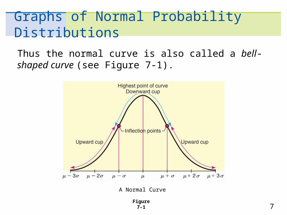
Thus the normal curve is also called a bell-shaped curve (see Figure 7-1).

Figure 7-1

A Normal Curve

8


We see that a general normal curve is smooth and symmetrical about the vertical line extending upward from the mean .

Notice that the highest point of the curve occurs over . If the distribution were graphed on a piece of sheet metal, cut out, and placed on a knife edge, the balance point would be at .

We also see that the curve tends to level out and approach the horizontal (x axis) like a glider making a landing.

9


However, in mathematical theory, such a glider would never quite finish its landing because a normal curve never touches the horizontal axis.

The parameter controls the spread of the curve. The curve is quite close to the horizontal axis at + 3 and – 3.

Thus, if the standard deviation is large, the curve will be more spread out; if it is small, the curve will be more peaked.

10


Figure 7-1 shows the normal curve cupped downward for an interval on either side of the mean .

Figure 7-1

A Normal Curve

11


Then it begins to cup upward as we go to the lower part of the bell. The exact places where the transition between the upward and downward cupping occur are above the points + and – .

In the terminology of calculus, transition points such as these are called inflection points.

12


The parameters that control the shape of a normal curve are the mean and the standard deviation . When both and are specified, a specific normal curve is determined. In brief, locates the balance point and determines the extent of the spread.

13


14


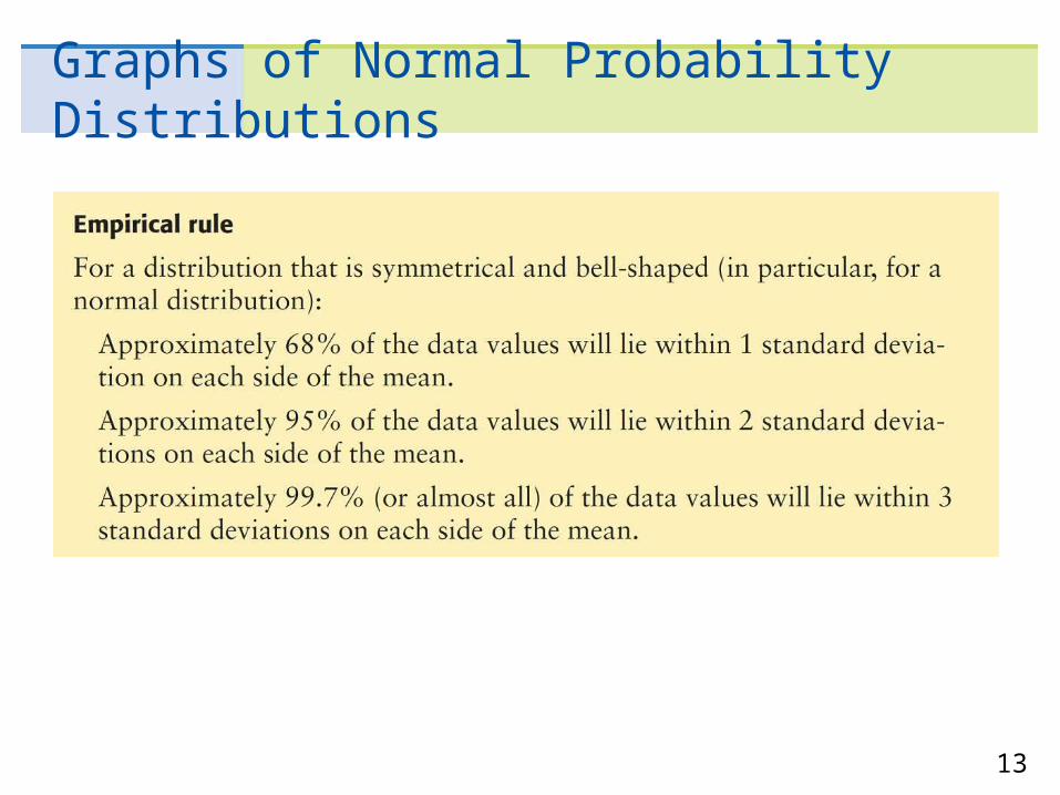
The preceding statement is called the empirical rule because, for symmetrical, bell-shaped distributions, the given percentages are observed in practice.

Furthermore, for the normal distribution, the empirical rule is a direct consequence of the very nature of the distribution (see Figure 7-3).

Figure 7-3Area Under a Normal Curve

15


Notice that the empirical rule is a stronger statement than Chebyshev’s theorem in that it gives definite percentages, not just lower limits.

Of course, the empirical rule applies only to normal or symmetrical, bell-shaped distributions, whereas Chebyshev’s theorem applies to all distributions.

16

Example 1 – Empirical rule

The playing life of a Sunshine radio is normally distributed with mean = 600 hours and standard deviation = 100 hours.

What is the probability that a radio selected at random will last from 600 to 700 hours?

17

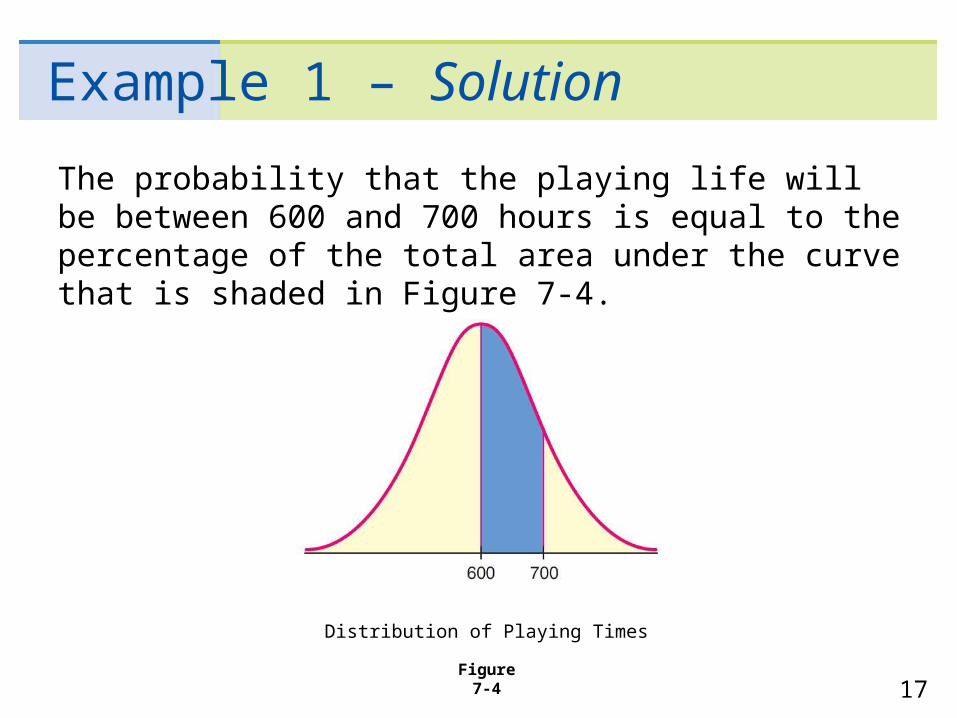
Example 1 – Solution

The probability that the playing life will be between 600 and 700 hours is equal to the percentage of the total area under the curve that is shaded in Figure 7-4.

Figure 7-4

Distribution of Playing Times

18

Example 1 – Solution

Since = 600 and + = 600 + 100 = 700, we see that the shaded area is simply the area between and + .

The area from to + is 34% of the total area.

This tells us that the probability a Sunshine radio will last between 600 and 700 playing hours is about 0.34.

cont’d

Copyright © Cengage Learning. All rights reserved. Normal Curves and Sampling Distributions 7.

Documents

Transcript of Copyright © Cengage Learning. All rights reserved. Normal Curves and Sampling Distributions 7.