Copyright © Cengage Learning. All rights reserved. Exponential Function Modeling and Graphs SECTION...

Copyright © Cengage Learning. All rights reserved.

Exponential Function Modeling and Graphs

SECTION 6.2

2

Learning Objectives

1 Construct exponential models algebraically from tables or words

2 Use exponential regression to model real-world data sets

3 Graph exponential functions given in equations, tables, or words

3

Modeling with Constant Percentage Rates of Change

4

Example 1 – Creating an Exponential Model from a Verbal Description

According to the World Health Organization, 538 thousand ITNs were distributed in the African region in 1999. In 2003, 9485 thousand nets were distributed. Between 1999 and 2003, net distribution increased at a nearly constant percentage rate.

a.) Find the function that models the distribution.

b.) Forecast the number of nets that will be distributed in 2011.

c.) Explain whether or not the estimate is realistic.

5



a.) Find the function that models the distribution.

6



b.) Forecast the number of nets that will be distributed in 2011.

7



c.) Explain whether or not the estimate is realistic.

8

Example 1 – Solution

Let t be the number of years since 1999 and let n be the number of nets distributed (in thousands).

Since the distribution of nets is anticipated to increase at a constant percentage rate, we can use an exponential model.

Since t = 0 corresponds with 1999, the initial value is 538. So far we have Although the growth factor is not readily apparent, we can calculate it by substituting the second data point into the equation.

9


Since 2003 corresponds with t = 4, we have

Thus the exponential model is .

To determine the net distribution level in 2011, we evaluate this function at t = 12.

cont’d

10


According to the model, 2,946,000 thousand (2.946 billion) nets will be distributed in 2011.

Although the model gives a good estimate for years near the original data set, the further we move away from 2003, the less confident we are in the prediction because few things can sustain exponential growth indefinitely.

Since 2011 is relatively far away from the last year in the data set (2003), we question the accuracy of the forecast.

cont’d

11

Modeling Half-Life and Doubling Time

12

Radioactive substances such as polonium-210 decay exponentially. The half-life of polonium-210 is 138.376 days (138 days, 9 hours, 1 minute, and 26 seconds).

(Remember: The half-life of a substance is the amount of time it takes for half of the initial amount of the substance to remain.)

Polonium-210 has a half-life of 138.376 days. What percentage of the substance decays each day?

Modeling Half-Life and Doubling Time

13

Example 3 – Determining a Percentage Rate of Decay from a Half-Life

Solution:Since the substance is decaying exponentially, we can model the amount remaining by Since half of the initial value remains after 138.376 days, we have

Since b = 1 + r, r = –0.005. The amount of polonium-210 remaining is decreasing at a rate of 0.5% per day.

14

Example 5 – Determining If Data Can Be Represented by an Exponential Model

Doubling time is the amount of time it takes for something that is growing to double. As was the case with half-life, doubling time is independent of the initial value of the exponential function.

15

Example 5 – Determining If Data Can Be Represented by an Exponential Model

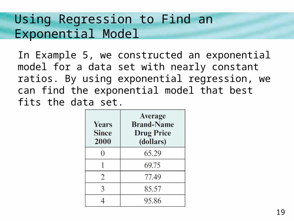
a.) Use the table to determine if an exponential model is appropriate for this data. b.) If so, model the data with an exponential function andc.) estimate the average drug price in 2006.

Table 6.11

16


Since the input values are equally spaced, we need only determine if consecutive output values have a constant ratio. See Table 6.12.

The ratios are all approximately equal to 1.1, so they are nearly constant. Thus an exponential model is appropriate for this data set.

Table 6.12

17


Using 65.29 as the initial value, we construct an exponential model

where t is the number of years since 2000.

To determine the average drug price in 2006, we evaluate the function at t = 6.

According to the model, the average brand-name drug price in 2006 was $115.70.

cont’d

18

Using Regression to Find an Exponential Model

19

In Example 5, we constructed an exponential model for a data set with nearly constant ratios. By using exponential regression, we can find the exponential model that bestfits the data set.


20

Using regression we find the exponential model is;

Using the model of best fit, we get a slightly different estimate for the average brand-name prescription drug price in 2006.

Versus 115.70 using constant ratios.


21

Example 6 – Using Exponential Regression to Model a Data Set

Find the equation of the exponential function that best fits the data set shown in Table 6.13. Then forecast the U.S. exports to Colombia in 2010.

Table 6.13

22


Using the Technology Tip at the end of this section, we obtain

where t is the number of years since the end of 1990.

To forecast exports in 2010, we evaluate the function at t = 20.

We estimate that U.S. exports to Colombia will be $1228 million in 2010.

23

Graphing Exponential Functions

24

The growth factor plays a significant role in determining the shape of the graph of an exponential function. Let’s investigate its effect in the context of economic forecasting.


25

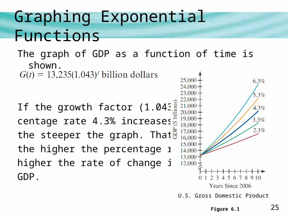
The graph of GDP as a function of time is shown.

If the growth factor (1.043) or per-

centage rate 4.3% increases,

the steeper the graph. That is,

the higher the percentage rate, the

higher the rate of change in the

GDP.


Figure 6.1

U.S. Gross Domestic Product

26

We also see that although the difference between the projections for 2016 is substantial, the difference in the projections for 2007 is relatively small.

Thus, the change factor tells us much about the graph. We have known that the change factor b is equivalent to 1 plus the percentage change rate. That is, b = 1 + r.


27


28

Inflation refers to the increase in prices that occurs over time.

For example, if the annual inflation rate is 3% then an item that costs $100 today will cost 100 + 100(0.03) = $103 a year from now.

Consider the price of the chic leather boots for women in 1911, they cost $3.79. A comparable boot, retailed for $57.00 in 2011.

Example 8 – Interpreting Exponential Function Graphs

29

a. Determine the average annual inflation rate for the boots.

b. Graph an exponential function model for the price of the boots.

c. Estimate the price of the boots in 1963 and 2003 from the graph.

Example 8 – Interpreting Exponential Function Graphscont’d

30

We first need to determine the ratio of the prices.

The 2011 price was about 15 times more than the 1911 price.

To determine the annual growth factor, we raise this number to 1 over the length of the period between 1911 and 2011 (100 years).

Example 8(a) – Solution

31

We subtract 1 from the growth factor to obtain the annual percentage change rate.

The average annual rate of inflation on the boots was about 2.75%.

Example 8(a) – Solutioncont’d

32

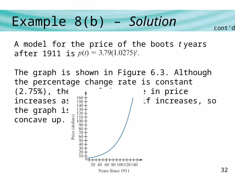
A model for the price of the boots t years after 1911 is The graph is shown in Figure 6.3. Although the percentage change rate is constant (2.75%), the annual increase in price increases as the price itself increases, so the graph is

concave up.

Example 8(b) – Solutioncont’d

33

In 1963, t = 52. From the graph it appears as if the boot price was approximately $15 in 1963. In 2003, t = 92.

From the graph it appears as if the boot price was approximately $46 in 2003.

Example 8(c ) – Solutioncont’d

Copyright © Cengage Learning. All rights reserved. Exponential Function Modeling and Graphs SECTION...

Documents

Transcript of Copyright © Cengage Learning. All rights reserved. Exponential Function Modeling and Graphs SECTION...