Copyright © Cengage Learning. All rights reserved. 3 Derivatives.
24
Copyright © Cengage Learning. All rights reserved. 3 Derivatives
-
Upload
prince-kimbel -
Category
Documents
-
view
220 -
download
2
Transcript of Copyright © Cengage Learning. All rights reserved. 3 Derivatives.

Copyright © Cengage Learning. All rights reserved.
3 Derivatives
Copyright © Cengage Learning. All rights reserved.
3.3Derivatives of Trigonometric
Functions
33
Derivatives of Trigonometric Functions
In particular, it is important to remember that when we talk about the function f defined for all real numbers x by
f (x) = sin x
it is understood that sin x means the sine of the angle whose radian measure is x. A similar convention holds for the other trigonometric functions cos, tan, csc, sec, and cot.
All of the trigonometric functions are continuous at every number in their domains.
44
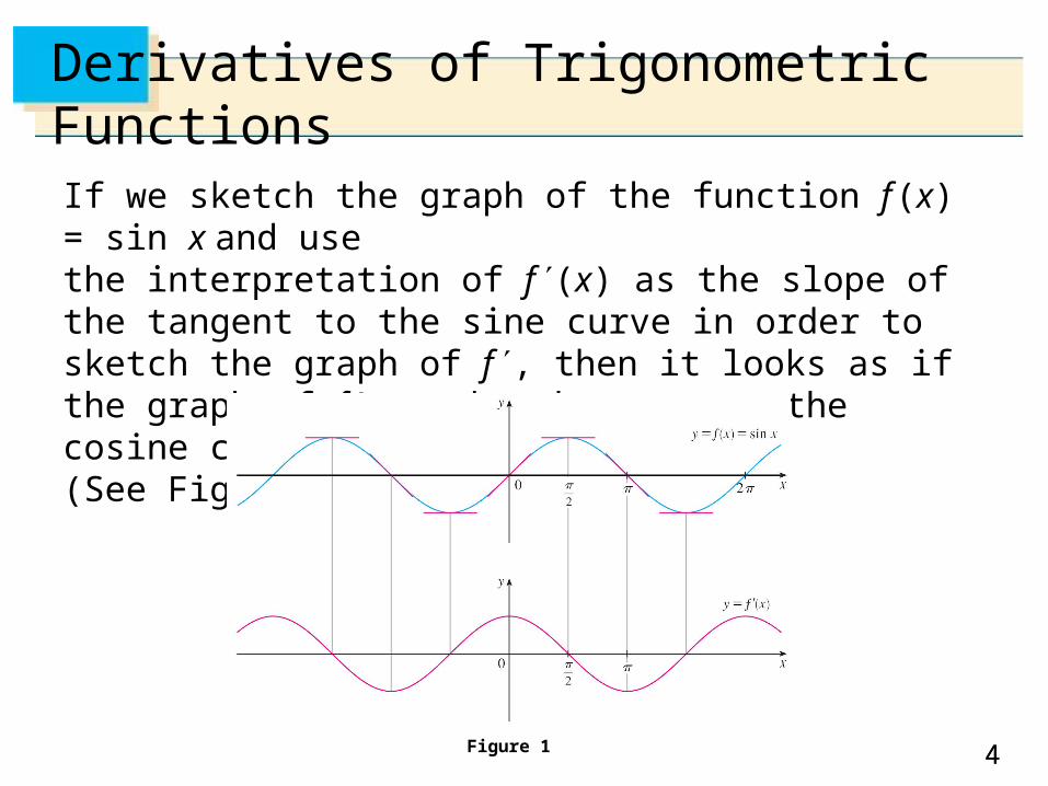
Derivatives of Trigonometric Functions
If we sketch the graph of the function f (x) = sin x and usethe interpretation of f (x) as the slope of the tangent to the sine curve in order to sketch the graph of f , then it looks as if the graph of f may be the same as the cosine curve.(See Figure 1).
Figure 1
55
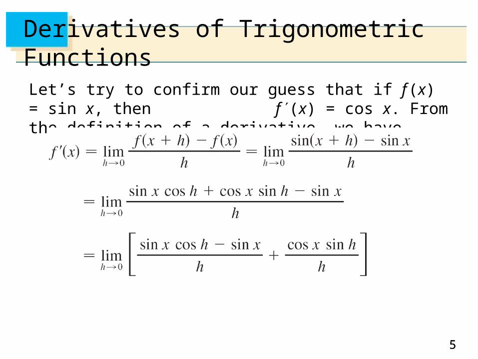
Derivatives of Trigonometric Functions
Let’s try to confirm our guess that if f (x) = sin x, then f (x) = cos x. From the definition of a derivative, we have
66
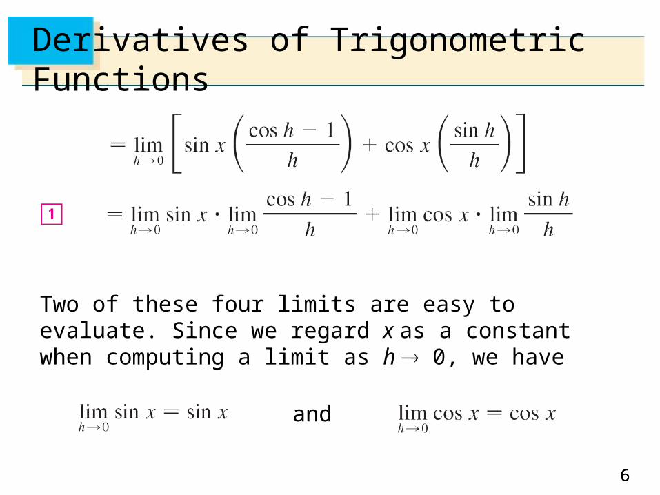
Derivatives of Trigonometric Functions
Two of these four limits are easy to evaluate. Since we regard x as a constant when computing a limit as h 0, we have
and
77
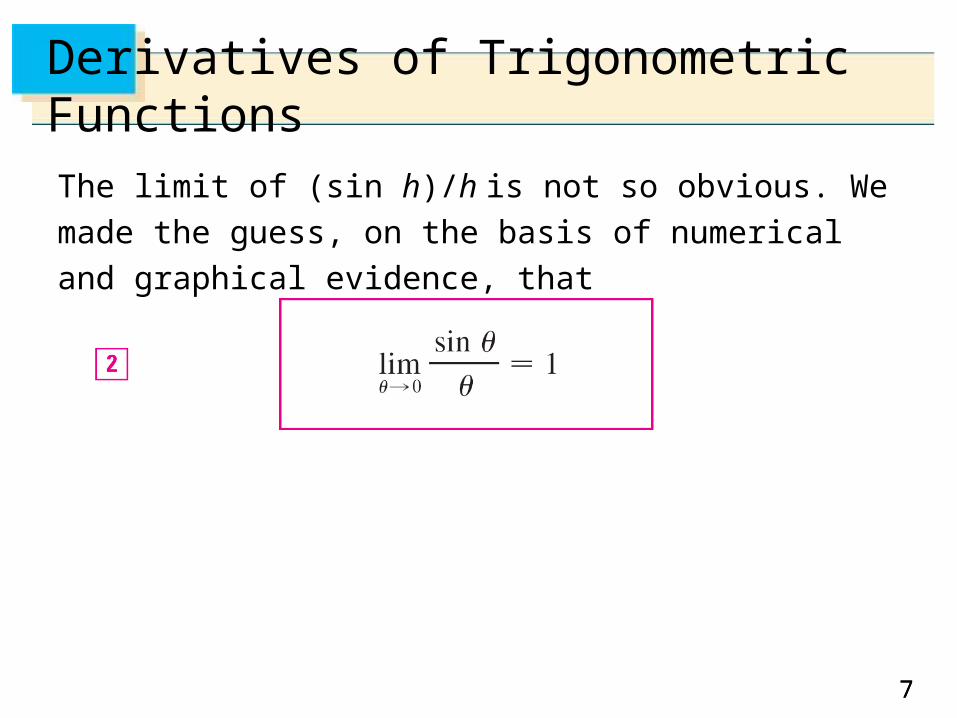
Derivatives of Trigonometric Functions
The limit of (sin h)/h is not so obvious. We made the guess,
on the basis of numerical and graphical evidence, that

88
Derivatives of Trigonometric Functions
We now use a geometric argument to prove Equation 2. Assume first that lies between 0 and /2. Figure 2(a) shows a sector of a circle with center O, central angle , and radius 1.
BC is drawn perpendicular to OA.By the definition of radian measure, we have arc AB = . Also | BC | = | OB | sin = sin .
Figure 2(a)
99
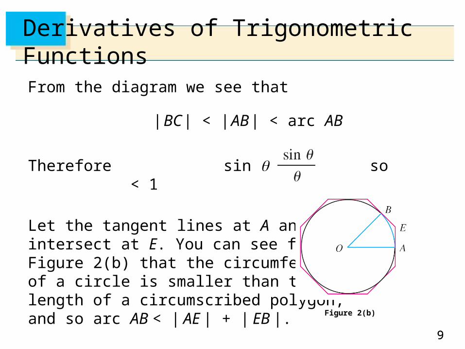
Derivatives of Trigonometric Functions
From the diagram we see that
| BC | < | AB | < arc AB
Therefore sin < so < 1
Let the tangent lines at A and Bintersect at E. You can see from Figure 2(b) that the circumference of a circle is smaller than the length of a circumscribed polygon, and so arc AB < | AE | + | EB |.
Figure 2(b)
1010
Derivatives of Trigonometric Functions
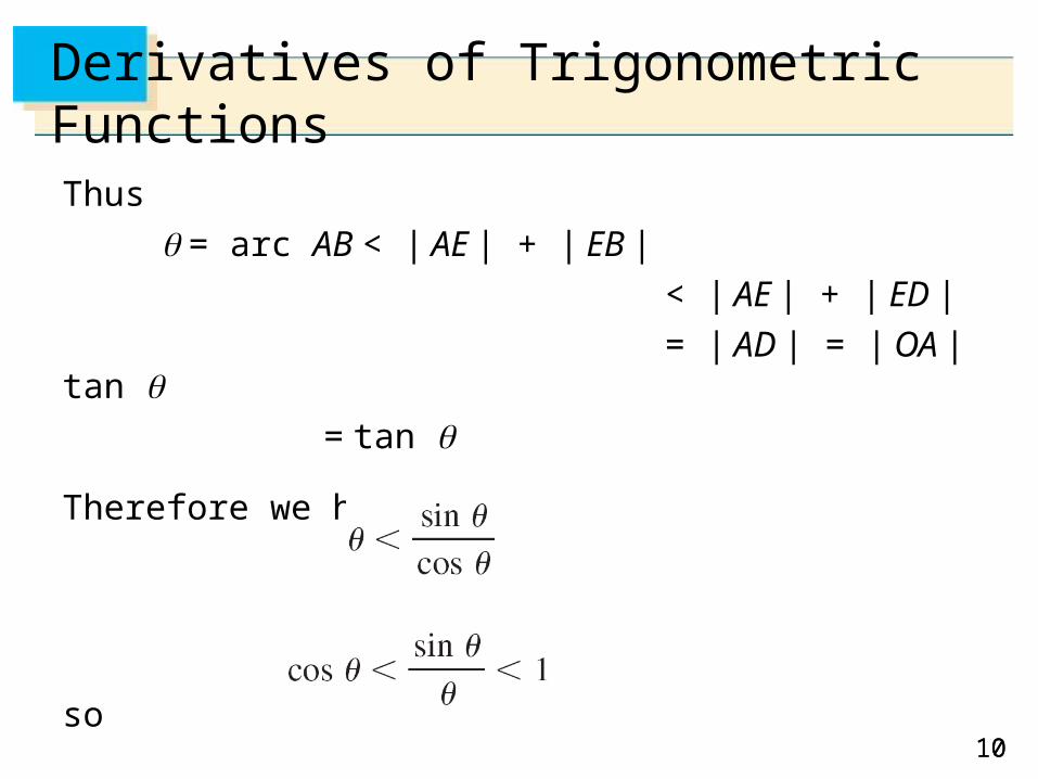
Thus
= arc AB < | AE | + | EB |
< | AE | + | ED |
= | AD | = | OA | tan = tan
Therefore we have
so
1111
Derivatives of Trigonometric Functions
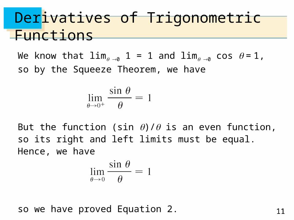
We know that lim 0 1 = 1 and lim 0 cos = 1, so by the
Squeeze Theorem, we have
But the function (sin )/ is an even function, so its right and left limits must be equal. Hence, we have
so we have proved Equation 2.
1212
Derivatives of Trigonometric Functions
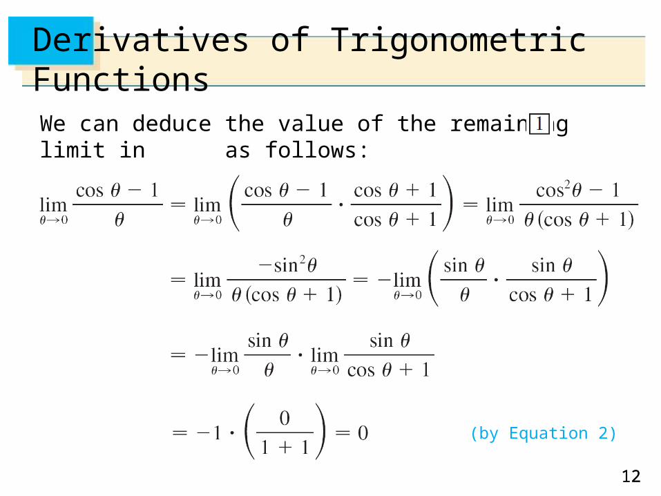
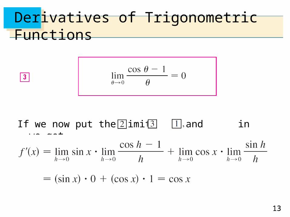
We can deduce the value of the remaining limit in as follows:
(by Equation 2)
1313
Derivatives of Trigonometric Functions
If we now put the limits and in we get

1414
Derivatives of Trigonometric Functions
So we have proved the formula for the derivative of the sine
function:
1515
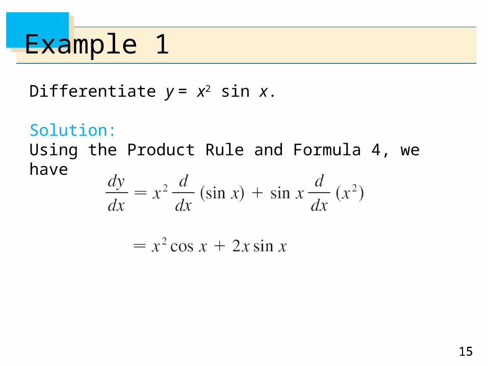
Example 1
Differentiate y = x2 sin x.
Solution:Using the Product Rule and Formula 4, we have

1616
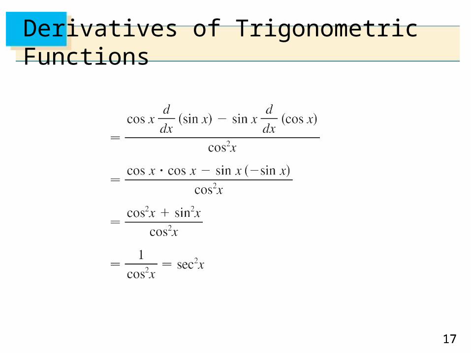
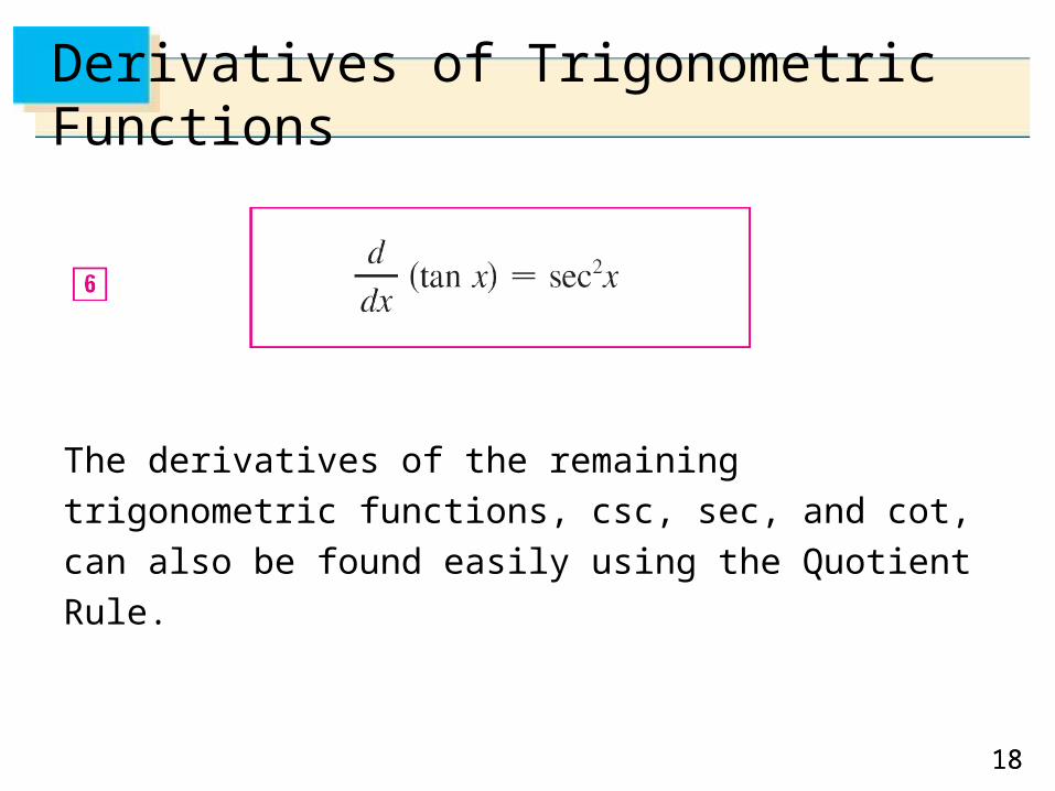
Derivatives of Trigonometric Functions
Using the same methods as in the proof of Formula 4, one can prove that
The tangent function can also be differentiated by using the definition of a derivative, but it is easier to use the Quotient Rule together with Formulas 4 and 5:
1717
Derivatives of Trigonometric Functions
1818
Derivatives of Trigonometric Functions
The derivatives of the remaining trigonometric functions,
csc, sec, and cot, can also be found easily using the
Quotient Rule.
1919
Derivatives of Trigonometric Functions
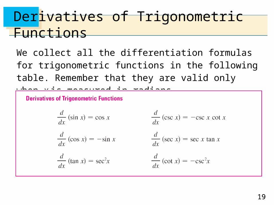
We collect all the differentiation formulas for trigonometric functions in the following table. Remember that they are valid only when x is measured in radians.
2020
Derivatives of Trigonometric Functions
Trigonometric functions are often used in modeling
real-world phenomena. In particular, vibrations, waves,
elastic motions, and other quantities that vary in a periodic
manner can be described using trigonometric functions. In
the following example we discuss an instance of simple
harmonic motion.
2121
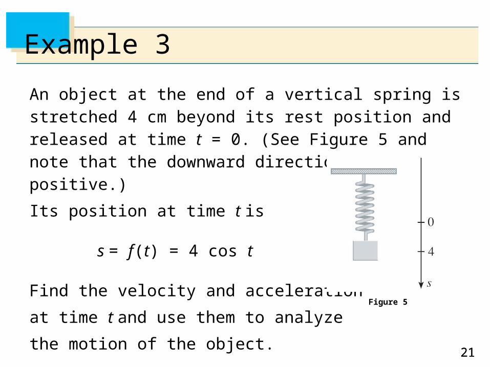
Example 3
An object at the end of a vertical spring is stretched 4 cm beyond its rest position and released at time t = 0. (See Figure 5 and note that the downward direction is positive.)
Its position at time t is
s = f (t) = 4 cos t
Find the velocity and acceleration
at time t and use them to analyze
the motion of the object. Figure 5
2222
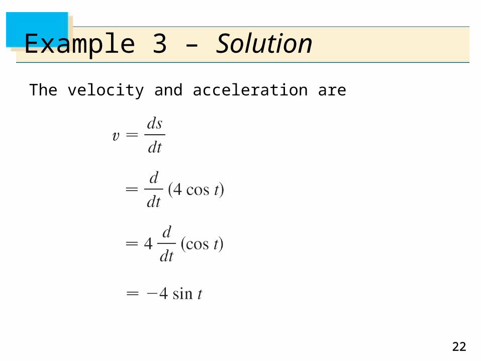
Example 3 – Solution
The velocity and acceleration are
2323
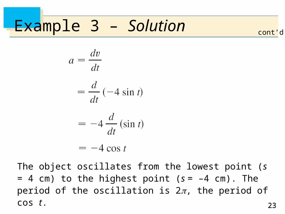
Example 3 – Solution
The object oscillates from the lowest point (s = 4 cm) to the highest point (s = –4 cm). The period of the oscillation is 2, the period of cos t.
cont’d
2424
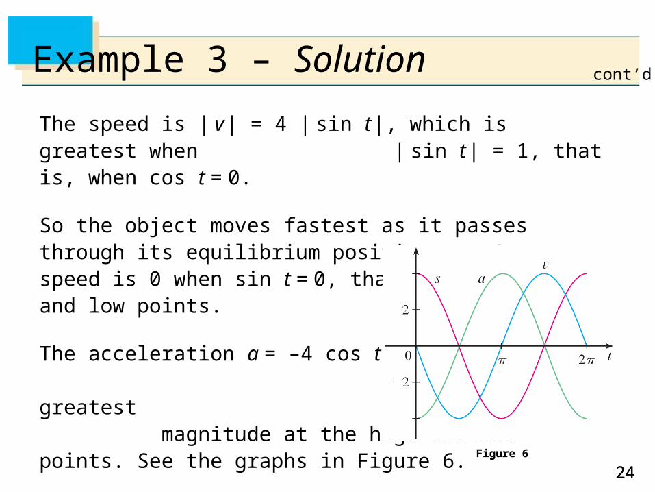
Example 3 – Solution
The speed is | v | = 4 | sin t |, which is greatest when | sin t | = 1, that is, when cos t = 0.
So the object moves fastest as it passes through its equilibrium position (s = 0). Its speed is 0 when sin t = 0, that is, at the high and low points.
The acceleration a = –4 cos t = 0 when s = 0. It has greatest magnitude at the high and low points. See the graphs in Figure 6.
Figure 6
cont’d