Copyright (c) Tom Kuppens. All rights reserved. No part of ... › publication › 472290 › file...
352
Copyright (c) Tom Kuppens. All rights reserved. No part of this work may be reproduced; any quotations must acknowledge the source.
Transcript of Copyright (c) Tom Kuppens. All rights reserved. No part of ... › publication › 472290 › file...

Copyright (c) Tom Kuppens. All rights reserved. No part of this work may be reproduced; any quotations must acknowledge the source.

TOM KUPPENS
development of methodology to assign
absolute configurations using vibrational
circular dichroism
promotor: Prof. Dr. P. Bultinck, Ghent University
co-promotor: Prof. Dr. W. Herrebout, University of Antwerp
Dissertation for the degree of Doctor in Sciences: Chemistry – December 2006 Ghent University, Faculty of Sciences Department of Inorganic and Physical Chemistry


And now for something completely different. – Monty Python's Flying Circus

v
table of contents List of publications xi Abbreviations xiii
1 INTRODUCTION_________________________________________________ 1
1.1 Absolute configuration___________________________________________ 1 1.2 Vibrational circular dichroism _____________________________________ 4 1.3 Aim _________________________________________________________ 6 1.4 Reference list __________________________________________________ 9
2 VCD INTENSITIES ______________________________________________ 13
2.1 Introduction __________________________________________________ 13 2.2 VCD theory __________________________________________________ 14 2.2.1 Problem outline______________________________________________ 14 2.2.2 Born-Oppenheimer approximation and beyond _____________________ 17 2.2.3 Vibronic coupling transition moments ____________________________ 23 2.2.4 Atomic polar tensors __________________________________________ 27 2.2.5 Magnetic field perturbation_____________________________________ 28 2.2.6 Dipole and rotational strengths __________________________________ 32 2.3 Implementation _______________________________________________ 32 2.3.1 Approximation methods _______________________________________ 32 2.3.1.1 Hartree-Fock ______________________________________________ 33 2.3.1.2 Density functional theory_____________________________________ 35 2.3.2 Gauge invariance ____________________________________________ 39 2.3.3 Analytical derivates___________________________________________ 41 2.4 Reference list _________________________________________________ 46

vi
3 MEASUREMENT OF VCD ________________________________________ 51
3.1 Introduction __________________________________________________ 51 3.2 VCD spectrometer _____________________________________________ 52 3.2.1 Circularly polarized light creation _______________________________ 53 3.2.2 Signal detection______________________________________________ 55 3.2.3 Calibration__________________________________________________ 57 3.3 Experimental procedure _________________________________________ 59 3.4 Reference list _________________________________________________ 62
4 COMPARISON OF SPECTRA _____________________________________ 65
4.1 Introduction __________________________________________________ 65 4.2 Simulation of spectra ___________________________________________ 66 4.3 Assignment of fundamentals _____________________________________ 67 4.4 Spectral comparison____________________________________________ 69 4.4.1 Correlation functions__________________________________________ 69 4.4.2 Generalized expression for similarity _____________________________ 74 4.4.3 Neighborhood similarity _______________________________________ 76 4.4.4 Numerical integration _________________________________________ 78 4.5 Reference list _________________________________________________ 80
5 DETERMINATION OF THE STEREOCHEMISTRY OF HYDROXYMETHYL DIHYDRODIOXINOPYRIDINE BY VCD AND THE EFFECT OF DFT INTEGRATION GRIDS_________________ 81
5.1 Introduction __________________________________________________ 81 5.2 Experimental _________________________________________________ 83 5.3 Computational methodology _____________________________________ 85 5.4 Results and discussion __________________________________________ 88 5.4.1 Conformational analysis _______________________________________ 88 5.4.2 Single conformational spectra___________________________________ 93 5.4.3 Boltzmann weighted spectra ____________________________________ 98 5.5 Conclusion __________________________________________________ 106 5.6 Reference list ________________________________________________ 108

vii
6 DETERMINATION OF THE AC OF THREE as-HYDRINDACENE COMPOUNDS BY VCD _______________________________________ 111
6.1 Introduction _________________________________________________ 111 6.2 Results and discussion _________________________________________ 113 6.2.1 Synthesis __________________________________________________ 113 6.2.2 IR and VCD spectroscopy_____________________________________ 114 6.2.3 Computational methods ______________________________________ 115 6.2.4 Theoretical spectra __________________________________________ 117 6.2.5 Conformational analysis ______________________________________ 117 6.2.6 IR and VCD spectra _________________________________________ 122 6.3 Conclusion __________________________________________________ 134 6.4 Supplementary material index ___________________________________ 134 6.5 Reference list ________________________________________________ 136
7 ELUCIDATION OF THE AC OF JNJ-27553292, A CCR2 RECEPTOR ANTAGONIST _______________________________________________ 139
7.1 Introduction _________________________________________________ 139 7.2 Methods ____________________________________________________ 142 7.2.1 Preparation of the catalyst_____________________________________ 142 7.2.2 Preparation of (+)-(R)-1-(3’,4’-dichlorophenyl)-propanol ____________ 142 7.2.3 Preparation of (−)-(S)-4-(1-azidopropyl)-1,2-dichlorobenzene ________ 143 7.2.4 Preparation of (−)-(S)-1-(3’,4’-dichlorophenyl)-propanamine ________ 143 7.2.5 Spectroscopy _______________________________________________ 144 7.2.6 Computation _______________________________________________ 144 7.2.7 Conformational analysis ______________________________________ 145 7.2.8 IR and VCD data____________________________________________ 148 7.3 Results and discussion _________________________________________ 149 7.4 Conclusion __________________________________________________ 160 7.5 Supplementary material index ___________________________________ 160 7.6 Reference list ________________________________________________ 161
8 SELF-ASSOCIATION BEHAVIOR OF CARBOXYLIC ACIDS IN SOLUTION: A VCD PERSPECTIVE___________________________ 165
8.1 Introduction _________________________________________________ 165

viii
8.2 Intermolecular association of tetrahydrofuran-2-carboxylic acid in solution: a vibrational circular dichroism study____________________ 167
8.2.1 Introduction________________________________________________ 167 8.2.2 Experimental methods________________________________________ 168 8.2.3 Computational methods ______________________________________ 169 8.2.4 Conformational search _______________________________________ 169 8.2.5 Results and discussion _______________________________________ 173 8.2.6 Conclusion ________________________________________________ 186 8.2.7 Supplementary material index _________________________________ 186 8.3 Elucidation of the absolute configuration of
tetrahydrofuran-3-carboxylic acid ________________________________ 188 8.3.1 Introduction________________________________________________ 188 8.3.2 Experimental _______________________________________________ 188 8.3.3 Computational methods ______________________________________ 189 8.3.4 Results and discussion _______________________________________ 189 8.3.4.1 Conformational description __________________________________ 189 8.3.4.2 IR and VCD spectra ________________________________________ 192 8.3.4.3 Fundamental assignment ____________________________________ 195 8.3.4.4 Absolute configuration assignment ____________________________ 198 8.3.5 Conclusion ________________________________________________ 198 8.4 A DFT conformational analysis and VCD study on methyl-tetrahydrofuran-2-carboxylate _____________________________ 199 8.4.1 Scope and significance _______________________________________ 199 8.4.2 Introduction________________________________________________ 199 8.4.3 Methods___________________________________________________ 200 8.4.3.1 Preparation of (+)-(S)-methyl-tetrahydrofuran-2-carboxylate ________ 200 8.4.3.2 Spectroscopy _____________________________________________ 201 8.4.3.3 Computation______________________________________________ 202 8.4.4 Results and discussion _______________________________________ 202 8.4.5 Conclusion ________________________________________________ 218 8.4.6 Supplementary material index _________________________________ 218 8.5 Summary ___________________________________________________ 219 8.6 Reference list ________________________________________________ 220
9 NEIGHBORHOOD BASED ENANTIOMERIC SIMILARITY INDEX ____ 225
9.1 Introduction _________________________________________________ 225

ix
9.2 Enantiomeric similarity index ___________________________________ 227 9.3 Results _____________________________________________________ 228 9.3.1 Scaling factor ______________________________________________ 233 9.3.2 Basis set __________________________________________________ 234 9.3.3 Functional _________________________________________________ 235 9.3.4 Absolute configuration assignment and quality ____________________ 236 9.3.5 Diastereomer assignment _____________________________________ 239 9.4 Conclusion __________________________________________________ 241 9.5 Reference list ________________________________________________ 242
SUMMARY AND CONCLUSIONS __________________________________ 245
SAMENVATTING ________________________________________________ 253
1 Inleiding ____________________________________________________ 253 2 Vibrationeel circulair dichroïsme_________________________________ 254 3 Doelstelling van dit onderzoekswerk______________________________ 255 4 Samenvatting van de resultaten en conclusie________________________ 256
APPENDIX UNREPORTED AC ASSIGNMENTS ______________________ 263
Background ______________________________________________________ 263 Reference list_____________________________________________________ 273 Acknowledgements
xi
list of publications
The following papers have been published as a direct consequence of the work undertaken for this thesis:
Determination of the stereochemistry of 3-hydroxymethyl-2,3-dihydro-[1,4]dioxino[2,3-b]pyridine by vibrational circular dichroism and the effect of DFT integration grids Kuppens, T.; Langenaeker, W.; Tollenaere, J. P.; Bultinck, P. Journal of Physical Chemistry A 2003, 107, 542-553 Determination of absolute configuration via vibrational circular dichroism Kuppens, T.; Bultinck, P.; Langenaeker, W. Drug Discovery Today: Technologies 2004, 1, 269-275 Determination of the absolute configuration of three as-hydrindacene compounds by vibrational circular dichroism Kuppens, T.; Vandyck, K.; Van der Eycken, J.; Herrebout, W.; van der Veken, B. J.; Bultinck, P. Journal of Organic Chemistry 2005, 70, 9103-9114 Elucidation of the absolute configuration of JNJ-27553292, a CCR2 receptor antagonist, by vibrational circular dichroism analysis of two precursors Kuppens, T.; Herrebout, W.; van der Veken, B. J.; Corens, D.; De Groot, A.; Doyon, A.; Van Lommen, G.; Bultinck, P. Chirality 2006, 18, 609-620 Intermolecular association of tetrahydrofuran-2-carboxylic acid in solution: A vibrational circular dichroism study Kuppens, T.; Herrebout, W.; van der Veken, B. J.; Bultinck, P. Journal of Physical Chemistry A 2006, 100, 10191-10200

xii
A DFT conformational analysis and VCD study on methyl tetrahydrofuran-2-carboxylate Kuppens, T.; Vandyck, K.; Van der Eycken, J.; Herrebout, W.; van der Veken, B. J.; Bultinck, P. Spectrochimica Acta Part A-Molecular and Biomolecular Spectroscopy 2006, Published online. Structure elucidation of polychloroterpenes obtained from optically active pinenes: 2-endo,5,5,8,8,9,9,10,10,10-decachlorofenchane by NMR and (1R,3S,4S,5S,6S,7R)-2,2,3-exo,5-endo,6-exo,8,9,9,10,10-decachlorobornane by VCD Kruchkov, F. A.; Kuppens, T.; Kolehmainen, E.; Nikiforov, V. A. Organohalogen Compounds 2006, 68 In press I was responsible for the VCD measurements/calculations and the absolute configuration assignment Vibrational circular dichroism DFT study on bicyclo[3.3.0]octane products Debie, E.; Kuppens, T.; Vandyck, K.; Van der Eycken, J.; van der Veken, B. J.; Herrebout, W.; Bultinck, P. Submitted to Tetrahedron-Asymmetry 2006 I was responsible for the conformational analysis, measurements and calculation of the spectra for all four compounds
The following papers have been published outside the scope of this thesis: Quantum similarity superposition algorithm (QSSA): A consistent scheme for molecular alignment and molecular similarity based on quantum chemistry Bultinck, P.; Kuppens, T.; Girone, X.; Carbo-Dorca, R. Journal of Chemical Information and Computer Sciences 2003, 43, 1143-1150 I was responsible for the Fortran code testing A selected ion flow tube study of the reactions of H3O+, NO+ and O2
.+ with some oxygenated biogenic volatile organic compounds Amelynck, C.; Schoon, N.; Kuppens, T.; Bultinck, P.; Arijs, E. International Journal of Mass Spectrometry 2005, 247, 1-9 I was responsible for the conformational analysis and property calculations for all eight compounds

xiii
abbreviations
AAT atomic axial tensor AC absolute configuration APT atomic polar tensor BO Born-Oppenheimer CPHF coupled perturbed Hartree-Fock DFT density functional theory ECD electronic circular dichroism EMEA European agency for the evaluation of medicinal
products ESI enantiomeric similarity index FDA food and drug administration (US) FTIR Fourier transformed IR GGA generalized gradient approximation GIAO gauge including/invariant atomic orbitals HF Hartree-Fock IR infrared KS Kohn-Sham LDA local density approximation LIA lock-in amplifier LOA London atomic orbitals LP linearly polarized MCT mercury cadmium telluride (detector) MFP magnetic field perturbation MO molecular orbital MP2 second-order Møller-Plesset perturbation theory NDA new drug application NMR nuclear magnetic resonance NS neighborhood similarity

xiv
OR optical rotation PEM photoelastic modulator PES potential energy surface RCP/LCP right/left circularly polarized S/N signal-to-noise ratio SCF self consistent field THF tetrahydrofuran VCD vibrational circular dichroism VCT vibronic coupling theory XRD X-ray diffraction ZPD zero path difference

References p.9 1
1 introduction
1.1 Absolute configuration
In recent years, a considerable interest in the biological activity of the enantiomers of chiral drugs has emerged.1 This interest in drug stereochemistry has resulted from the considerable advances in the synthesis, analysis and separation of chiral molecules.2 There are numerous examples in literature that show that enantiomers of chiral drugs, differ substantially in their biological properties.3 In chiral drugs, one enantiomer is often responsible for a given pharmacological activity, whereas the other may be less active, inactive, toxic, or may give rise to an entirely different pharmacological response.4 As a result of these advances in technology and the benefits of single enantiomer drugs, drug stereochemistry became an issue for the pharmaceutical industry and the regulatory authorities. In 1992, the Food and Drug Administration (FDA) in the USA published a policy statement5 for the development of new stereoisomeric drugs, which was closely followed by guidelines from the European Agency for the Evaluation of Medicinal Products (EMEA) in 1993.

Chapter 1
2
At present, there is no absolute requirement from any of the regulatory authorities for the development of single enantiomer drugs, and the decision of the stereoisomeric form to be developed (racemic or single enantiomer) is left to the applicant. The applicant however, must recognize the occurrence of chirality in new drugs; attempt to separate the stereoisomers, assess the contribution of the various stereoisomers to the activity of interest and make a rational selection of the stereoisomer that is proposed for marketing.6 An illustration of a drug for which a single active enantiomer was developed from a previously marketed racemate, is ibuprofen. The main analgesic activity of ibuprofen resides predominantly in the S enantiomer.7 Administration of the racemate, (R)-ibuprofen results in a biologically fortuitous metabolic chiral inversion to the active S enantiomer.8
CO2H HO2C
(R)-(–)-ibuprofen (S)-(+)-ibuprofen Figure 1.1 Enantiomers of ibuprofen.
Regulatory bodies such as the FDA and EMEA are responsible for approving whether a drug can proceed to clinical trials and whether it should be allowed to be marketed. In order to get the new drug on the market in the US, a pharmaceutical company has to submit a New Drug Application (NDA) to the FDA. The applicant has to file an exhaustive report which details on the drug compound.9 Evidently, structural information on the drug compound is also an important issue. For chiral drugs, the structural information provided needs to describe the absolute configuration (AC)10 of the active molecule. Not only the regulatory bodies demand such information on chiral drugs. If a pharmaceutical company wants to secure their intellectual properties for a potent compound in the early stages of the drugs discovery process, absolute configurations of the key compounds need to be known.11,12 Research scientists are also interested

Introduction
References p.9 3
in the stereochemical structure of their enantiomers. The absolute configuration of chiral compounds is critical in understanding structure-activity relationships13 or in the development for appropriate chiral separations14, resolutions, or syntheses. Also, in a synthesis process, chemists always want to know the absolute configuration of their precursors and synthesized compounds as early as possible. Given the combination of the rapidly growing market for chiral drugs and the general need to determine absolute configurations of the chiral molecules, there is evidently a need for tools that allow accessible absolute configuration determining. The primary tool for determining absolute configurations is single-crystal X-ray diffraction (XRD) measurements using anomalous scattering.10,15,16 This requires high-quality single crystals and additionally, the crystal should be subject to anomalous scattering which, for standard XRD experiments, can be obtained by introducing heavy atoms in the crystal. These conditions are not always met. Other methods are nuclear magnetic resonance (NMR),17,18 optical rotation,19-23 stereospecific synthesis and electronic circular dichroism (ECD).23-26 The latter technique is a form of UV/VIS spectroscopy that relies on the differential absorption of a chiral molecule towards left and right circularly polarized light.27 In order to be applicable, the compound needs specific functional groups, that is, chromophores that can absorb UV/VIS radiation. A relative new technique in this context is vibrational circular dichroism (VCD), which combines the structural specificity of IR spectroscopy with the stereochemical sensitivity of circular dichroism. In Table 1.1 an overview is given in which the most applied techniques are given with their advantages and disadvantages.28

Chapter 1
4
Table 1.1 Comparison of different techniques that can be applied for absolute configuration determination
advantage disadvantage vi
brat
iona
l ci
rcul
ar
dich
rois
m
(VC
D) - applicable in solution on
a wide range of molecules
- measurements are not straightforward
X-r
ay
diff
ract
ion
(XR
D)
- reliable - regulatory standard
- need for good quality single crystals and dispersive scatters
nucl
ear
mag
netic
re
sona
nce
(NM
R)
- well known - need for chiral shift reagents,
chiral additives or derivatization
optic
al
rota
tion
(OR
) - relatively easy to measure
- higher level calculations needed compared to VCD
- only one property can be compared in contrast to VCD (comparison of spectra)
- sign depends on solvent used
elec
tron
ic
circ
ular
di
chro
ism
(E
CD
)
- applicable on molecules in solution
- only a few bands are available
1.2 Vibrational circular dichroism
Chiral molecules interact differently with left and right circularly polarized radiation (Figure 1.2). The measurement of differential absorption of the incident radiation in the infrared region is known as vibrational circular dichroism (VCD).29 The significance of VCD lies in the fact that it provides a wealth of information on the structure and the stereochemistry of the chiral molecule as VCD intensities arise from vibrational transitions in a chiral molecule. In ordinary IR absorption spectra no stereochemical information is embedded. Because VCD is a differential

Introduction
References p.9 5
spectroscopy form, VCD intensities can be negative with the bands centered at the vibrational frequencies. Mirror image molecules have identical unpolarized IR absorption intensities, but have opposite VCD intensities. The latter is a reflection of the chiral nature of the compound that was measured. However, it does not provide any direct information on the actual absolute configuration.30
Figure 1.2 Differential absorption of RCP and LCP radiation by a chiral molecule. Before VCD was experimentally observed, theoretical studies and predictions of VCD were performed in the early 1970s, using empirical models.31-35 These theoretical predictions indicated that VCD intensities should be strong enough in order to be observed. This greatly encouraged and guided experimental observations of VCD. The earliest measurements of VCD were reported in 1973 by Holzwarth et al.36,37 In the next few years, more VCD measurements were reported in literature.38,39 The implementation of FTIR VCD by Nafie et al.40-43 in 1979 and further development in the instrumentation (see Chapter 3) nowadays allows the measurement high quality VCD spectra for most chiral compounds in solution. The interpretation and evaluation, that is, the process of extracting configurational and conformational information from experimental VCD spectra is not straightforward. For a reliable evaluation one needs calculated VCD spectra. Because a good theory was missing, a variety of empirical models emerged during the 1970s and 1980s that were applied to the analysis of the VCD spectra, with more or less success.44 Theoretical modeling of spectra, however, has been hampered by the complexities involved in the calculation of VCD intensities. VCD originates from interaction between radiation and charged particles taking into account the magnetic dipole interaction. The rotational strength (which is proportional to the VCD intensity) is a scalar product of the electric and magnetic dipole transition
Circularly polarised light Absorption
Difference ΔA=AL – AR
a
e
db

Chapter 1
6
moments (see Chapter 2). The traditional approach based on the Born-Oppenheimer approximation yields good values for the electric dipole transition moments (IR absorption intensities). However, evaluation of the magnetic dipole transition moment yields no electronic contribution when associated to vibrational transitions, which is physically unacceptable.45 In the mid 1980s a theory that permitted a priori prediction of VCD spectra was developed.46,47 This theory was implemented using ab initio computational methods.48,49 The first calculations48,50 were based on Hartree-Fock methods, which rendered insufficiently accurate spectra to permit comparison with experiment.51 Introduction of post-HF methods such as Møller-Plesset second order perturbation (MP2) provided general improvements in the simulated spectra, however, due the computational cost, this approximation was practically not feasible.52-54 The development of density functional theory (DFT) and the introduction of hybrid functionals55,56 in the early 1990s, meant a breakthrough for the calculation of VCD intensities. DFT methods provide a good accuracy, i.e. spectra comparable with experiment, and even more important, at a moderate computational cost.57 1.3 Aim
The scope of this thesis is the development of a methodology at the application level that allows the transparent calculation and measurement of VCD spectra, and ultimately the assignment of the AC. The implementation of VCD intensities at the DFT level of theory in Gaussian58, and the advent of the commercialization of VCD spectrometers meant that both theoretical calculations and the experimental methods were not longer restricted to the few specialist in the field. However, for VCD to become a practical technique for interested scientists, development is still needed. For some non-theoretical chemist, the barrier for using quantum chemical techniques is often rather high, and therefore the VCD technique needs to be made more accessible.
Introduction
References p.9 7
The main objectives of this study can be summarized as follows:
- Optimization of the calculation of VCD spectra and performance testing of different computational parameters for medium-sized/large molecules,
- gain insight in the measurement and interpretation of the VCD for organic synthesis and typical pharmaceutical drug compounds,
- introduce a method that allows a thorough, yet transparent and quick comparison of experimental and theoretical spectra.
The structure of this dissertation is organized in two major sections. The first part consists of Chapters 1 through 4. In Chapter 2 and 3 a general review is given of the fundamental principles of VCD as this research area was completely new to our group. In Chapter 2, the theory for the calculation of VCD intensities is outlined, whereas in Chapter 3 an overview of the experimental VCD measurements is given. Both the application of the experiment and theory are an essential part of this thesis. In Chapter 4 the simulation of the VCD spectra is explained. The principles of spectral comparison are introduced and spectral similarity measures are proposed. In the second part, the experimental results are given in chronological order. Chapter 5 describes the earliest study that was performed in cooperation with Johnson & Johnson Pharmaceutical Research and Development (JNJPRD). Here, the AC of a pharmaceutical compound was validated using VCD. The performance of various basis sets and density functional grids was studied. In Chapter 6, the ACs of three as-hydrindacene compounds were determined, in cooperation with the Department of Organic Chemistry of Ghent University. Chapter 7 describes an extensive study that was performed on two precursor molecules of a potent CCR2 receptor antagonist (JNJPRD), in order to determine the AC of the latter. In Chapter 8, the self-association of carboxylic acids is investigated using IR and VCD spectroscopy. Two position isomers of a tetrahydrofuroic acid and a corresponding methyl ester are studied. In Chapter 9, the enantiomeric similarity index is proposed, which gives information about the similarity of experimental and theoretical spectra. Throughout Chapter 5–8, different similarity measures are used. As the studies are presented chronologically, an evolution in the similarity measure (which was developed throughout the studies performed in this thesis) can be observed.

Chapter 1
8
In the Appendix, unpublished VCD assignments are presented, which were mostly performed for JNJPRD. Additionally, due to the extensive amount of comprehensive tables, spectra and other material, a Supplementary Material section is provided which is downloadable from the internet in PDF format: http://www.quantum.UGent.be/tksup.pdf

Introduction
9
1.4 Reference list
1. Caner, H.; Groner, E.; Levy, L.; Agranat, I. Drug Discovery Today 2004, 9,
105-110.
2. Rouhi, A. M. Chem. Eng. News 2004, 82, 47-62.
3. Szelenyi, I.; Geisslinger, G.; Polymeropoulos, E.; Paul, W.; Herbst, M.; Brune, K. Drug. News. Perspect. 1998, 11, 139-160.
4. Ariens, E. J. Med. Res. Rev. 1986, 6, 451-466.
5. Chirality 1992, 4, 338-340.
6. Branch, S. K. International Regulation of Chiral Drugs. In Chiral Separation Techniques, 2nd ed.; Subramanian, G., Ed.; Wiley-VCH: Weinheim, 2006; pp 319-342.
7. Adams, S. S.; Bresloff, P.; Mason, C. G. J. Pharm. Pharmacol. 1976, 28, 256-257.
8. Caldwell, J.; Hutt, A. J.; Fournel-Gigleux, S. Biochem. Pharmacol. 1988, 37, 105-114.
9. Patrick, G. Medicinal Chemistry; 1st ed.; BIOS Scientific Publishers Limited: Oxford, 2001.
10. Flack, H. D.; Bernardinelli, G. Acta. Crystallogr. A 1999, 55, 908-915.
11. Rouhi, A. M. Chem. Eng. News 2005, 83, 32-33.
12. Agranat, I.; Caner, H. Drug Discovery Today 1999, 4, 313-321.
13. Serilevy, A.; West, S.; Richards, W. G. J. Med. Chem. 1994, 37, 1727-1732.
14. Agrawal, Y. K.; Patel, R. Rev. Anal. Chem. 2002, 21, 285-316.
15. Bijvoet, J. M. Koninkl. Ned. Akad. Wetenschap. 1949, B52, 313-314.
16. Flack, H. D.; Bernardinelli, G. J. Appl. Crystallogr. 2000, 33, 1143-1148.
17. Hoye, T. R.; Hamad, A. S. S.; Koltund, O.; Tennakoon, M. A. Tetrahedron Lett. 2000, 41, 2289-2293.

Chapter 1
10
18. Hoye, T. R.; Koltun, D. O. J. Am. Chem. Soc. 1998, 120, 4638-4643.
19. Stephens, P. J.; McCann, D. M.; Cheeseman, J. R.; Frisch, M. J. Chirality 2005, 17, S52-S64.
20. Stephens, P. J.; Devlin, F. J.; Cheeseman, J. R.; Frisch, M. J. J. Phys. Chem. A 2001, 105, 5356-5371.
21. Polavarapu, P. L.; Petrovic, A.; Wang, F. Chirality 2003, 15, S143-S149.
22. Stephens, P. J.; Devlin, F. J.; Cheeseman, J. R.; Frisch, M. J.; Rosini, C. Org. Lett. 2002, 4, 4595-4598.
23. Specht, K. M.; Nam, J.; Ho, D. M.; Berova, N.; Kondru, R. K.; Beratan, D. N.; Wipf, P.; Pascal, R. A.; Kahne, D. J. Am. Chem. Soc. 2001, 123, 8961-8966.
24. Uray, G.; Verdino, P.; Belaj, F.; Kappe, C. O.; Fabian, W. M. F. J. Org. Chem. 2001, 66, 6685-6694.
25. Pescitelli, G.; Gabriel, S.; Wang, Y. K.; Fleischhauer, J.; Woody, R. W.; Berova, N. J. Am. Chem. Soc. 2003, 125, 7613-7628.
26. Vandyck, K.; Matthys, B.; Van der Eycken, J. Tetrahedron Lett. 2005, 46, 75-78.
27. Berova, N.; Nakanishi, K.; Woody, R. W. Circular Dichroism: Principles and Applications; 2nd ed.; Wiley-VCH: New York, 2000.
28. Kuppens, T.; Bultinck, P.; Langenaeker, W. Drug Discovery Today: Techn. 2004, 1, 269-275.
29. Nafie, L. A. Appl. Spectrosc. 1996, 50, A14-A26.
30. Polavarapu, P. L. Spectroscopy 1994, 9, 48-55.
31. Deutsche, C. W.; Moscowitz, A. J. Chem. Phys. 1968, 49, 3257-3272.
32. Deutsche, C. W.; Moscowitz, A. J. Chem. Phys. 1970, 53, 2630-2644.
33. Schellman, J. A. J. Chem. Phys. 1973, 58, 2882-2886.
34. Schellman, J. A. J. Chem. Phys. 1974, 60, 343.
35. Holzwart, G.; Chabay, I. J. Chem. Phys. 1972, 57, 1632-1635.

Introduction
11
36. Holzwart, G.; Hsu, E. C.; Mosher, H. S.; Faulkner, T. R.; Moscowit, A. J. Am. Chem. Soc. 1974, 96, 251-252.
37. Hsu, E. C.; Holzwart, G. J. Chem. Phys. 1973, 59, 4678-4685.
38. Nafie, L. A.; Keiderling, T. A.; Stephens, P. J. J. Am. Chem. Soc. 1976, 98, 2715-2723.
39. Nafie, L. A.; Cheng, J. C.; Stephens, P. J. J. Am. Chem. Soc. 1975, 97, 3842-3843.
40. Lipp, E. D.; Nafie, L. A. Appl. Spectrosc. 1984, 38, 20-26.
41. Lipp, E. D.; Zimba, C. G.; Nafie, L. A. Chem. Phys. Lett. 1982, 90, 1-5.
42. Nafie, L. A.; Diem, M. Appl. Spectrosc. 1979, 33, 130-135.
43. Nafie, L. A.; Diem, M.; Vidrine, D. W. J. Am. Chem. Soc. 1979, 101, 496-498.
44. Stephens, P. J.; Lowe, M. A. Annu. Rev. Phys. Chem. 1985, 36, 213-241.
45. Faulkner, T. R.; Marcott, C.; Moscowitz, A.; Overend, J. J. Am. Chem. Soc. 1977, 99, 8160-8168.
46. Stephens, P. J. J. Phys. Chem.-US 1985, 89, 748-752.
47. Stephens, P. J. J. Phys. Chem.-US 1987, 91, 1712-1715.
48. Lowe, M. A.; Stephens, P. J.; Segal, G. A. Chem. Phys. Lett. 1986, 123, 108-116.
49. Jalkanen, K. J.; Stephens, P. J.; Amos, R. D.; Handy, N. C. Chem. Phys. Lett. 1987, 142, 153-158.
50. Lowe, M. A.; Segal, G. A.; Stephens, P. J. J. Am. Chem. Soc. 1986, 108, 248-256.
51. Cheeseman, J. R.; Frisch, M. J.; Devlin, F. J.; Stephens, P. J. Chem. Phys. Lett. 1996, 252, 211-220.
52. Stephens, P. J.; Jalkanen, K. J.; Devlin, F. J.; Chabalowski, C. F. J. Phys. Chem.-US 1993, 97, 6107-6110.
53. Devlin, F. J.; Stephens, P. J. J. Am. Chem. Soc. 1994, 116, 5003-5004.

Chapter 1
12
54. Yang, D. Y.; Rauk, A. J. Chem. Phys. 1994, 100, 7995-8002.
55. Becke, A. D. J. Chem. Phys. 1993, 98, 5648-5652.
56. Stephens, P. J.; Devlin, F. J.; Chabalowski, C. F.; Frisch, M. J. J. Phys. Chem.-US 1994, 98, 11623-11627.
57. Stephens, P. J.; Devlin, F. J. Chirality 2000, 12, 172-179.
58. Frisch, M. J.; Trucks, G. W.; Schlegel, H. B.; Scuseria, G. E.; Robb, M. A.; Cheeseman, J. R.; Montgomery Jr, J. A.; Vreven, T.; Kudin, K. N.; Burant, J. C.; Millam, J. M.; Iyengar, S. S.; Tomasi, J.; Barone, V.; Mennucci, B.; Cossi, M.; Scalmani, G.; Rega, N.; Petersson, G. A.; Nakatsuji, H.; Hada, M.; Ehara, M.; Toyota, K.; Fukuda, R.; Hasegawa, J.; Ishida, M.; Nakajima, T.; Honda, Y.; Kitao, O.; Nakai, H.; Klene, M.; Li, X.; Knox, J. E.; Hratchian, H. P.; Cross, J. B.; Bakken, V.; Adamo, C.; Jaramillo, J.; Gomperts, R.; Stratmann, R. E.; Yazyev, O.; Austin, A. J.; Cammi, R.; Pomelli, C.; Ochterski, J. W.; Ayala, P. Y.; Morokuma, K.; Voth, G. A.; Salvador, P.; Dannenberg, J. J.; Zakrzewski, V. G.; Dapprich, S.; Daniels, A. D.; Strain, M. C.; Farkas, O.; Malick, D. K.; Rabuck, A. D.; Raghavachari, K.; Foresman, J. B.; Ortiz, J. V.; Cui, Q.; Baboul, A. G.; Clifford, S.; Cioslowski, J.; Stefanov, B. B.; Liu, G.; Liashenko, A.; Piskorz, P.; Komaromi, I.; Martin, R. L.; Fox, D. J.; Keith, T.; Al-Laham, M. A.; Peng, C. Y.; Nanayakkara, A.; Challacombe, M.; Gill, P. M. W.; Johnson, B.; Chen, W.; Wong, M. W.; Gonzalez, C.; Pople, J. A. Gaussian03, Revision B5; Gaussian, Inc.: Wallingford CT, 2004.
References p.46 13
2 vibrational circular
dichroism intensities Equation Chapter 2 Section 1 2.1 Introduction
In this chapter, an overview of the theory for the calculation of VCD intensities is given. The main emphasis is given to the derivation of a usable wave function that produces a non-zero electronic contribution to the magnetic dipole transition moment. The vibronic coupling theory of Nafie and Freedman and subsequently, the magnetic field perturbation theory of Stephens are introduced. The implementation and evaluation of the VCD expressions is discussed.

Chapter 2
14
2.2 VCD theory
2.2.1 Problem outline1,2
When a molecule is exposed to IR radiation with a frequency ω=2πυ, the molecule may undergo a vibrational transition if the energy difference between two vibrational states, say iΨ and fΨ , is ħω and the transition dipole moment is
non-zero. The transition dipole moment (or electric dipole transition moment) between states iΨ and fΨ is given as the integral
elec elec,if i f= Ψ Ψμ μ (2.1)
elecμ is the electric dipole moment operator and iΨ and fΨ are the total molecular
wave functions representing respectively the vibrational states i and f. The electric dipole moment operator is the sum of the electron (E) and nuclear (N) operators, E N
elec elec elec= +μ μ μ (2.2) with
Eelec
1
n
dd=
= −∑rμ (2.3)
and
Nelec
1
N
Zα αα=
= ∑μ R (2.4)
Working in atomic units, rd is the position of the d th electron, and Zα and Rα are the charge and position of the αth nucleus. n and N are respectively the number of electrons and nuclei. The integrated intensity of an IR band is directly proportional to the dipole strength D, which is obtained from the square of the electric dipole transition moment

VCD intensities
References p.46 15
2elecif i fD = Ψ Ψμ (2.5)
The dipole strength is related to the intensity of an IR absorption band3 through the extinction coefficient ε according to
399 184 10ifband
dD .
νεν
−= ⋅ ∫ (2.6)
where ν is the fundamental transition frequency in wave numbers. The units of Dif are esu2cm2. The extinction coefficient in molar absorptivity units is related to the absorbance A through Beer’s Law A lcε= (2.7) with l the path length (in cm) and c the molar concentration. Vibrational circular dichroism is formally defined as the difference in absorption by a chiral sample of left versus right circularly polarized IR radiation. L RA A AΔ = − (2.8)
Where AL and AR are the corresponding absorbances. The intensity of a VCD band is directly proportional to the vibrational rotational strength. For a transition between two vibrational states i and f of a chiral molecule in its ground electronic state, the rotational strength Rif is given by the imaginary part of the scalar product of the electric dipole and magnetic dipole transition moments elec magiif i f f iR = − Ψ Ψ Ψ Ψμ μ (2.9)
The imaginary part has to be taken because magμ is a purely imaginary operator.
The magnetic dipole moment operator is the sum of the electron and nuclear operators E N
mag mag mag= +μ μ μ (2.10)

Chapter 2
16
with
Emag
1
12
n
d dd c=
= − ×∑μ r p (2.11)
and
Nmag
1 2
N ZM c
αα α
αα== ×∑μ R P (2.12)
pd is the momentum of the d th electron, and Mα and Pα are the mass and momentum of the αth nucleus. c in Equations (2.11) and (2.12) is the speed of light. According to Equation (2.9) the rotational strength is positive or negative depending on the angles between the two transition vectors, i.e., it is positive if the angle
between the vectors is less than 2π , negative if the angle is greater than
2π and zero
if the angle is equal to 2π (or when elec,ifμ or mag,ifμ is zero).
The rotational strength is proportional to the integrated intensity of the VCD absorption band3 according to
392 296 10if
band
dR .
νεν
−= ⋅ Δ∫ (2.13)
The units of Rif are esu2cm2. εΔ is the differential molar absorptivity. Computation of IR and VCD intensities requires the evaluation of electric and magnetic transition moments. The total vibronic wave function can be approximated as the product of the vibrational ( gvχ ) and electronic ( gψ ) wave functions using
adiabatic Born-Oppenheimer4,5 (BO) functions ( ) ( ) ( )gv g gv, ;ψ χΨ = ⋅r R r R R (2.14)
with sub indexes g for the electronic state and v for the vibrational state. The electronic wave function depends on the electronic coordinate r and has a parametric dependence on the nuclear coordinate R, i.e., gψ is a function of r defined for fixed
values of R. The nuclear motion wave function gvχ is a function of R.

VCD intensities
References p.46 17
For a vibrational transition in the electronic and vibrational ground state (00) to the vibrationally excited state (01), the transition moments can be written as
E N00 elec 01 00 0 elec 0 elec 01( ) ( ; ) ( ) ( ; ) ( ) ( )χ ψ ψ χΨ Ψ = +μ R r R μ r r R μ R R (2.15)
E N
00 mag 01 00 0 mag 0 mag 01
N00 mag 01
( ) ( ; ) ( ) ( ; ) ( ) ( )
( ) ( ) ( )
χ ψ ψ χ
χ χ
Ψ Ψ = +
=
μ R r R μ r r R μ R R
R μ R R (2.16)
Because of the hermitian and imaginary nature of E
magμ together with the fact that
the singlet non-degenerate electronic ground state 0ψ can be chosen to be real, the electronic contribution to the magnetic dipole transition moment is cancelled,6 that is E
0 mag 0 0ψ ψ =μ (2.17)
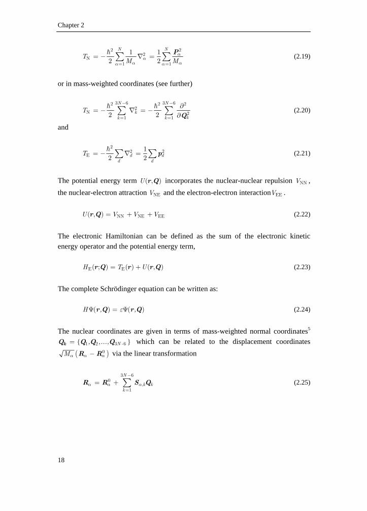
In order to include the important contributions from the electrons to the magnetic dipole transition moment, one has to choose either to make further approximations to the magnetic dipole operator yielding effective non-vanishing magnetic transition moments, or to go beyond the BO approximation. Various approximations7 are results of the former approach, which will not be discussed here. In the latter approach, more accurate wave functions are obtained by adding some corrections to the BO wave functions. 2.2.2 Born-Oppenheimer approximation and beyond2,8,9
The total molecular Hamiltonian H (2.18) is defined as the sum of the nuclear and electronic kinetic energy operator and the potential energy denoted respectively as
NT , ET and ( , )U r Q . E N( , ) ( ) ( , ) ( )H T U T= + +r Q r r Q Q (2.18)
with
Chapter 2
18
2 2
2N
1 1
1 12 2
N N
TM M
αα
α αα α= == − ∇ =∑ ∑ P (2.19)
or in mass-weighted coordinates (see further)
3 6 3 62 2 2
2N 2
1 12 2
N N
kkk k
T− −
= =
∂= − ∇ = −
∂∑ ∑ Q (2.20)
and
2
2 2E
12 2d d
d d
T = − ∇ =∑ ∑p (2.21)
The potential energy term ( , )U r Q incorporates the nuclear-nuclear repulsion NNV , the nuclear-electron attraction NEV and the electron-electron interaction EEV . NN NE EE( , )U V V V= + +r Q (2.22)
The electronic Hamiltonian can be defined as the sum of the electronic kinetic energy operator and the potential energy term, E E( ; ) ( ) ( , )H T U= +r Q r r Q (2.23)
The complete Schrödinger equation can be written as: ( ) ( )H , ,εΨ = Ψr Q r Q (2.24)
The nuclear coordinates are given in terms of mass-weighted normal coordinates5
{ }1 2 3 6N -, ,...,=kQ Q Q Q which can be related to the displacement coordinates
( )0Mα α α−R R via the linear transformation
3 6
0
1
N
,k kk
α α α
−
== + ∑R R S Q (2.25)

VCD intensities
References p.46 19
αR is the position vector of nucleus α (α=1,N) and 0αR is its equilibrium position.
,kαS is the displacement vector of the αth atom, incorporating the factor 1Mα
.
If it is assumed that the solutions of the electronic Schrödinger equation E ( ; ) ( ) ( ; )g g gH Eψ ψ=r Q Q r Q (2.26)
are known for sets of fixed values of Q , each set specifying a molecular configuration, the total wave function can be written as a linear combination of complete set of wave functions { }( )g ;ψ r Q .11
( ) ( ) ( )g g g
g
, ;χ ψΨ = ∑r Q Q r Q (2.27)
The total Schrödinger equation can then be written as
( )E N ( ) ( ) ( ) ( )g g g gg g
H T ; ;χ ψ ε χ ψ+ =∑ ∑Q r Q Q r Q (2.28)
and simplifying the expression
( )E N ( ) ( ) 0g gg
H T ;ε χ ψ+ − =∑ Q r Q (2.29)
The nuclear kinetic operator gives rise to the three following terms
( ) ( )N N N
2
( ) ( ) ( ) ( ) ( ) ( )
( ) ( )k kk
T ; T ; ; T
;
ψ χ ψ χ ψ χ
ψ χ
= +
− ∇ ∇∑r Q Q r Q Q r Q Q
r Q Q (2.30)
The introduction of Equation (2.30) in (2.29) yields
( ) 2N N( ) ( ) ( ) ( ) 0g g g k g k g
g k
; E T T ; ;ψ ε ψ ψ χ⎛ ⎞⎟⎜ + − + − ∇ ∇ =⎟⎜ ⎟⎟⎜⎝ ⎠∑ ∑r Q r Q r Q Q (2.31)

Chapter 2
20
If this expression is multiplied with ( )e ;ψ∗ r Q and integrating over the electronic coordinates, based on the orthonormality of the electronic eigenfunctions it can be written that
( )N N
2
( ) ( )( ) 0
( ) ( )
eg g e g
ge k g kg
k
E T ; T ;
; ;
δ ε ψ ψχψ ψ
⎛ ⎞+ − + −⎟⎜ ⎟⎜ ⎟⎜ =⎟⎜ ⎟∇ ∇⎜ ⎟⎟⎜⎝ ⎠∑ ∑
r Q r QQ
r Q r Q (2.32)
Separation of diagonal and non-diagonal terms gives ( )( )N N
2N
( ) ( ) ( )=
( ) ( ) ( ) ( ) ( )
e e e e
e g e k g k gg e k
E T ; T ;
; T ; ; ;
ε ψ ψ χ
ψ ψ ψ ψ χ≠
+ − +
⎛ ⎞⎟⎜− − ∇ ∇ ⎟⎜ ⎟⎟⎜⎝ ⎠∑ ∑
r Q r Q Q
r Q r Q r Q r Q Q (2.33)
The right-hand side of Equation (2.33) represents the coupling between electronic functions through nuclear motion. These terms are neglected in the adiabatic approximation. In adiabatic motion, electrons do not make transition from one electronic state to the other. Only the diagonal terms remain, i.e., ( )( )N N( ) ( ) ( ) ( )=0e e e eE T ; T ;ε ψ ψ χ+ − +Q r Q r Q Q (2.34) Which can also be written as [ ]( )N N( )+ ( ) ( ) ( )= ( )e e e ei ei eiT E ; T ;ψ ψ χ ε χ+ Q r Q r Q Q Q (2.35) where N( )+ ( ) ( )e e eE ; T ;ψ ψQ r Q r Q (2.36) represents the potential for nuclear motion. In Equation (2.35) a sub index i is introduced to distinguish the different eigenvalues and eigenfunctions for a given e. Neglecting the non-diagonal terms in Equation (2.33) corresponds to expressing the total wave function as an adiabatic product,

VCD intensities
References p.46 21
( ) ( ) ( )ei e ei, ;ψ χΨ =r Q r Q Q (2.37) In what is usually called the Born-Oppenheimer (BO) approximation, the expectation value of the nuclear kinetic energy over the electronic wave function given as the second term in Equation (2.36) is neglected. This is usually a good approximation because of the small electron to nuclear mass ratio. Within the BO approximation one can write the Schrödinger equation for the nuclear movement as ( )N ( ) ( ) ( )g gi gi giT E χ ε χ+ =Q Q Q (2.38)
The vibrational wave functions are eigenfunctions of ( )N ( )gT E+ Q with energy
giε . The electronic energy ( )gE Q serves as the potential for nuclear motion. The
vibrational wave function ( )giχ Q applies to the ith level of a vibration, for the gth
electronic state. It is supposed that this vibration corresponds to normal mode jQ
and all other normal vibrations are unaltered in the vibrational transition. The BO wave functions can be refined by retrieving the neglected terms from the nuclear kinetic energy
2 2
2N 2
E N E2k k kk k
T⎛ ⎞⎛ ∂ ⎞ ⎛ ∂ ⎞ ∂ ⎟⎜⎟ ⎟⎜ ⎜′ = − − ⎟⎟ ⎟ ⎜⎜ ⎜⎟ ⎟ ⎟⎜ ⎜ ⎟⎜⎝ ⎠ ⎝ ⎠∂ ∂ ⎝ ⎠∂∑ ∑Q Q Q
(2.39)
The differentiation subscripts E and N in Equation (2.39) indicate on which wave function the differential operator will operate. One can use NT ′ in Equation (2.39) as a perturbation operator to refine the BO wave functions, ( ) ( ) ( ) ( ) ( ) ( )gi g gi ev,gi e ev
ev gi
, ; a ;ψ χ ψ χ≠
Ψ = + ∑r Q r Q Q Q r Q Q (2.40)
where the coefficients are defined, on the basis of Rayleigh-Schrödinger perturbation theory, as

Chapter 2
22
N( ) ( ) ( ) ( )( )
( ) ( )e ev g gi
ev,gigi ev
; T ;a
E Eψ χ ψ χ′
=−
r Q Q r Q QQ
Q Q (2.41)
This approach is the non-adiabatic or BO vibronic coupling mechanism. The adiabatic electronic wave function gψ can be expanded as a function of its
nuclear dependence using as a starting point the crude adiabatic approximation.5,10 Here, the crude adiabatic wave functions are written as 0( ) ( ) ( )gi g gi, ;ψ χΨ =r Q r Q Q (2.42)
The only nuclear dependence is now contained in the vibrational wave function
( )giχ Q which is subtly different compared to its adiabatic counterpart because gψ is
defined here as nuclear independent. Using perturbation theory the nuclear dependence is reintroduced in the electronic wave function,
0
0 0
0 00 0
( )( ) ( )
( ) ( ) ( )( ) ( )
e gk
g g k eg ee g k
U ,; ;
; ; ;E E
ψ ψψ ψ ψ=
≠
∂∂
= + ⋅−∑∑ Q Q
r Qr Q r Q
Qr Q r Q Q r Q
Q Q
(2.43)
The notation 0k =
∂∂ Q QQ
indicates that the derivatives are evaluated at equilibrium
geometry. Equation (2.43) can be written more elegantly as
0
0( )
( ) ( ) gg g k
kk
;; ;
ψψ ψ
=
∂= + ⋅
∂∑Q Q
r Qr Q r Q Q
Q (2.44)
This expression can be interpreted as a Taylor expansion about the equilibrium geometrie of the electronic wave function, truncated to the linear term. This equation is also known as the Herzberg-Teller coupling12 or adiabatic coupling as electron and nuclear wave functions can still be separated,

VCD intensities
References p.46 23
0
0( )
( ) ( ) ( )ggi g k gi
kk
;, ;
ψψ χ
=
⎛ ⎞∂ ⎟⎜ ⎟⎜Ψ = + ⋅ ⎟⎜ ⎟∂ ⎟⎜⎝ ⎠∑
Q Q
r Qr Q r Q Q Q
Q (2.45)
Using Equations (2.44), (2.40) and (2.41) and neglecting higher order terms one obtains following expression for the wave function of interest for VCD,
0
0
0
02
0
( )( ) ( ) ( )
( ) ( )( ) ( )
( ) ( )( ) ( )
ggi g gi k gi
kk
g gie ev
k ke ev
ev gik ev gi
;;
;;
;E E
ψψ χ χ
ψ χψ χ
ψ χ
=
=
≠
∂Ψ = + ⋅
∂
∂ ∂∂ ∂
+−
∑
∑ ∑
Q Q
Q Q
r Qr Q Q Q Q
Q
r Q Qr Q Q
Q Qr Q Q
Q Q
(2.46) 2.2.3 Vibronic coupling transition moments2,8
In the previous paragraph a BO corrected wave function was derived using adiabatic and non-adiabatic coupling. If we introduce a general operator θ, which represents a radiation field interaction operator, the transition moment between vibronic states gi →gf can be written as gi gfθΨ Ψ . θ can be written as the sum of an electronic and
a nuclear part
N Eθ θ θ= + (2.47) The nuclear terms of the transition moment, i.e., N
gi gfθΨ Ψ can be written as
N N( ) ( )gi gf gi gfθ χ θ χΨ Ψ = Q Q (2.48)
An electronic contribution to the transition moment can be introduced using the wave functions as given in (2.46). Retaining only first order terms, the electronic transition moment E
gi gfθΨ Ψ can be written as
Chapter 2
24
0
0
0
E E0 0
E0
0 E0
02
0
( ) ( ) ( ) ( )
( )( ) ( ) ( )
( )( ) ( ) ( )
( ) ( )( ) ( )
( )( ) ( )
gi gf g gi g gf
gg gi k gf
kk
gk gi g gf
kk
g gfe ev
k kg
ev gfk ev gf
; ;
;;
;;
;;
;E E
θ ψ χ θ ψ χ
ψψ χ θ χ
ψχ θ ψ χ
ψ χψ χ
ψ χ
=
=
=
≠
Ψ Ψ =
∂+ ⋅ ⋅
∂
∂+ ⋅ ⋅
∂
∂ ∂∂ ∂
+−
∑
∑
∑ ∑
Q Q
Q Q
Q Q
r Q Q r Q Q
r Qr Q Q Q Q
Q
r QQ Q r Q Q
Q
r Q Qr Q Q
Q Qr Q
Q Q
0
E0
02 E
0 0
( ) ( ) ( )
( ) ( )( ) ( )
( ) ( ) ( ) ( )( ) ( )
gi e ev
g gie ev
k ke ev g gf
ev gik ev gi
;
;;
; ;E E
θ ψ χ
ψ χψ χ
ψ χ θ ψ χ=
≠
∂ ∂∂ ∂
+−∑ ∑ Q Q
Q r Q Q
r Q Qr Q Q
Q Qr Q Q r Q Q
Q Q
(2.49)
The first term of Equation (2.49) is not expected to contribute to the vibrational transition moment as no overlap is possible between the vibrational levels of the same electronic state. As a consequence this term vanishes. The remaining terms
contribute nuclear dependence to the vibrational integrals through Q and ∂∂Q
. If
the assumption is made that the energy difference between electronic-vibronic levels are approximately equal to the separation between electronic levels regardless of the vibrational excitations, it can be written that 0 0( ) ( ) ( ) ( )ev gf e gE E E E− = −Q Q Q Q (2.50)
This approximation is based on the fact that energy differences between vibrational states are much smaller than between electronic states. Under such an approximation one is able to formally close the sum over the vibronic wave functions in the fourth and fifth terms in (2.49) and it can be written as
0 0
0
0
E
E E0 0
02 E
0 00 0
02
( ) ( )( ) ( ) ( ) ( )
( ) ( )( ) ( )
( ) ( )( ) ( )
( )( ) (
gi gf
g gg g gi gf
k kk k
g gfe gi
k kg e
e gk e g
eg gf
k
; ;; ;
;;
; ;E E
;;
θ
ψ ψψ θ θ ψ χ χ
ψ χψ χ
ψ θ ψ
ψψ χ
= =
=
≠
=
Ψ Ψ =
⎛ ⎞∂ ∂ ⎟⎜ ⎟⎜ + ⎟⎜ ⎟∂ ∂ ⎟⎜⎝ ⎠
∂ ∂∂ ∂
+−
∂∂
+
∑ ∑
∑∑
Q Q Q Q
Q Q
Q Q
r Q r Qr Q r Q Q Q Q
Q Q
r Q Qr Q Q
Q Qr Q r Q
Q Q
r Qr Q Q
QE
0 00 0
( ))
( ) ( )( ) ( )
gi
ke g
e gk e g
; ;E E
χ
ψ θ ψ≠
∂∂
−∑∑
r Q r QQ Q
(2.51)

VCD intensities
References p.46 25
Equation (2.51) represents the principal sources of vibronic coupling in molecules, i.e., the first term is traditionally8 regarded as adiabatic whereas the last two terms are considered non-adiabatic and beyond the BO approximation. At this stage, the interaction operator introduced in Equation (2.47) can be specified so that for both the electric and magnetic dipole transition moment equations can be put forward. If Equation (2.51) is evaluated using the electric dipole operator, that is, if
E Eelecθ = μ the non-adiabatic terms will cancel. This is due to the anti-symmetric
property of the ∂∂Q
operator with respect to the interchange of wave functions
gi gf gf giχ χ χ χ∂ ∂
= −∂ ∂Q Q
(2.52)
Also, because E
elecμ is hermitian and it can be written that E E
elec elecg e e gψ ψ ψ ψ=μ μ (2.53)
For the same reason the adiabatic terms are equal. Combining Equations (2.48) and (2.51) the expression for the electric dipole transition moment becomes
0
Nelec elec
E0 elec
( ) ( )
( )2 ( ) ( ) ( )
gi gf gi gf
gg gi gf
kk
;;
χ χ
ψψ χ χ
=
Ψ Ψ =
∂+
∂∑Q Q
Q Q
r Qr Q Q Q Q
Q
μ μ
μ
(2.54) As indicated before, the non-adiabatic terms cancel and Equation (2.54) is entirely attributable to Herzberg-Teller coupling. This means that the electronic contribution to the induced dipole moment, which is the result of charge distribution changes induced by vibrational transitions, can be properly described by introducing explicit nuclear position dependence to the ground electronic wave function.

Chapter 2
26
For the magnetic dipole transition moment the first two terms will cancel because of the anti-symmetric property of the integrals by wave function interchange because
Emagμ is hermitian and imaginary
E E
mag magg e e gψ ψ ψ ψ= −μ μ (2.55)
The non-adiabatic terms are equal, so the expression of the magnetic dipole transitions becomes
0
Nmag mag
E0 mag 0 0
2
0 0
( ) ( )
( )( ) ( ) ( )
( )2 ( )
( ) ( )
gi gf gi gf
gg e e
k gfgi
e g kk e g
;; ; ;
E E
χ χ
ψψ ψ ψ
χχ=
≠
Ψ Ψ =
∂∂ ∂
+− ∂∑∑ Q Q
Q Q
r Qr Q r Q r Q
Q QQ
Q Q Q
μ μ
μ
(2.56) In this expression a non-vanishing electronic contribution to the magnetic dipole moment is obtained which comes from BO coupling. In Equation (2.56) it can be seen that excited electronic states are involved (“sum over states”). The electronic part of the induced magnetic moment is caused by the changes of the motion state of the electrons which are a direct response to the changes in the nuclear momentum. The response to the ground electronic state is described by mixing excited electronic states into the unperturbed ground electronic state wave functions.2 Expressions (2.54) and (2.56) describe the electronic and magnetic dipole transitions moments within the vibronic coupling theory (VCT) of Nafie and Freedman.8 Evaluation of the magnetic dipole transition moment as expressed in (2.56) has been implemented at ab initio level.13 Results from this implementation, however, do not seem to converge with increasing basis set size.14 In this work, a different approach is used for the evaluation of the magnetic dipole transition moment, i.e., the magnetic field perturbation theory of Stephens9 which is discussed further. First, expressions for the evaluation of the electronic dipole transition moment are derived.

VCD intensities
References p.46 27
2.2.4 Atomic polar tensors2,9
For the electronic dipole transition moment a more classical approach can be used which yields an expression formally equal to Expression (2.54) for the electronic dipole transition moment within the vibronic coupling theory. The quantity expressed in (2.15), i.e., E N
elec elec elecg
g gψ ψ + ≡μ μ μ , is the adiabatic
electric dipole moment of the ground state. Its nuclear coordinate dependence, in terms of a particular vibrational normal mode, may be expressed as a Taylor expansion about the equilibrium geometry, to the first order:
0
0
elecelec elec
gg g
==
∂= + ⋅
∂Q QQ Q
μμ μ Q
Q (2.57)
0
0
elecelec
elec,
( ) ( )
2
g
gi gf gi j gf
g
jj
ααα
χ χ
ω
=
=
∂Ψ Ψ =
∂
∂=
∂∑
Q Q
R R
μμ Q Q Q
Q
μS
R
(2.58)
Writing it in vector components, with β the Cartesian component of the electric field and λ the Cartesian component of the nuclear coordinates,
elec,elec, ,
0
,
2
2
g
gi gf jj
jj
μμ S
R
S
ββ αλ
αλα λ
αλβ αλ
α λ
ω
ω
∂Ψ Ψ =
∂
=
∑∑
∑∑P
(2.59)
In the above expression, the atomic polar tensor (APT) of nucleus α is introduced and given by
elec,
0
gμ
Rβα
λβαλ
∂=
∂P (2.60)
The APT was first introduced by Morcillo et al.15-18 Later, Person and Newton19 reviewed the properties of APTs.

Chapter 2
28
Because elecelec
gg gψ ψ=μ μ , α
λβP can be separated in a nuclear and electronic
part,
E0 elec,
0
( )2 ( ) g
g;
; ZR
αλβ β α λβ
αλ
ψψ μ δ
∂= +
∂P
r Rr R (2.61)
2.2.5 Magnetic field perturbation9,20
The infinite sum over electronic wave functions can be circumvented by invoking the magnetic field dependence of the wave function in Stephens’ magnetic field perturbation (MFP) approach for calculating rotational strengths. The external uniform magnetic field dependence of the wave function may be treated in an explicit manner. The magnetic field dependence of the electronic ground state can be expressed as a Taylor expansion, truncated after the linear term,
00 0 0
0
( )( ) ( ) g
g g,
, ,ψ
ψ ψ=
∂= + ⋅
∂ B
Q BQ B Q B B
B (2.62)
B is the magnetic induction vector associated to the external magnetic field represented by vector potential A. The derivatives in the second term of Equation (2.62) are evaluated in absence of the magnetic field (zero magnetic field, 0 0=B ). The perturbed electronic Hamiltonian in the presence of a magnetic field perturbation21 can be written to the first order: E
E E 0 mag( ) ( )H H= − ⋅B B Bμ (2.63)
with E 0( )H B the unperturbed Hamiltonian in absence of a magnetic field and the
first order perturbation Hamiltonian E( )H ′ B given by E
E mag( )H ′ = − ⋅B Bμ (2.64)
One can write the electronic ground state wave function, using a perturbation series with the perturbation E( )H ′ B as

VCD intensities
References p.46 29
0 E 0
0 0 0 0 00 0
( ) ( )( ) ( ) ( )
( ) ( )e g
g g eg ee g
, H ,, , ,
E Eψ ψ
ψ ψ ψ≠
′= + ⋅
−∑ 0 0Q B Q BQ B Q B Q B
Q Q (2.65)
Combining (2.62) and (2.65), one may identify the relation
E0 mag 00
0 00 00
( ) ( )( )( )
( ) ( )e gg
eg ee g
, ,,,
E E
ψ ψψψ
≠=
∂= −
∂ −∑B
Q B Q BQ BQ B
B Q Qμ
(2.66)
Insertion of (2.66) in the electronic part of (2.56) yields
0
0E 2mag
0
( ) ( ) ( )2 ( )g g gf
gi gf gik kk
,ψ ψ χχ
= =
∂ ∂ ∂Ψ Ψ = −
∂ ∂ ∂∑B Q Q
Q B Q QQ
B Q Qμ
(2.67) Invoking the harmonic oscillator nuclear wave functions, a number of simplifications are possible. The potential energy of the ground state can be written as
3 6
20
1
1( ) ( )
2
N
g g k kk
E E κ−
== + ∑Q Q Q (2.68)
jκ is the eigenvalue of the Hessian in Expression (2.69) using the transformation in
(2.25).
( ) ( )
0
2
0 0gE
α α α α′ ′
∂
∂ − ∂ −R=R
R R R R (2.69)
Each normal coordinate jQ is associated with a frequency j jω κ= . For the 0 → 1
excitation of the jth vibrational normal mode, it is known that
2( ) ( )22
gf gigi j gf
jj
E E
wχ χ
ω−
= =Q Q Q (2.70)
with

Chapter 2
30
01 00 jE E ω− = (2.71)
Also, using the commutator relationship
[ ] 2N,j
jT
∂=
∂Q
Q (2.72)
it can be written that
( ) ( )2
jgi gf
j
ωχ χ
∂=
∂Q Q
Q (2.73)
If k is taken equal to j, Equation (2.67) can be written as2
0
0E 2mag
0
( ) ( ) ( )2 ( )g g gf
gi gf gij j
,ψ ψ χχ
= =
∂ ∂ ∂Ψ Ψ = −
∂ ∂ ∂B Q Q
Q B Q QQ
B Q Qμ (2.74)
Taking into account Expression (2.73) and the transformation in Equation (2.25);
0
0
0E 2mag
0
30
0
( ) ( ) ( )2 ( )
( ) ( )2
2
g g gfgi gf gi ,j
j
j g g,j
,
,
ααα
ααα
ψ ψ χχ
ω ψ ψ
= =
= =
∂ ∂ ∂Ψ Ψ = −
∂ ∂ ∂
∂ ∂= −
∂ ∂
∑
∑
B R R
B R R
R B R QQ S
B R Q
R B RS
B R
μ (2.75)
Emagμ can further be written in vector components, where β is the Cartesian
component of the uniform magnetic field and λ is the Cartesian component of the nuclear coordinates.
0
30E
mag,0
( ) ( )2
2j g g
gi gf ,j,
SB Rβ αλβ αλα
ω ψ ψ
==
∂ ∂Ψ Ψ = −
∂ ∂∑R RB
R B Rμ (2.76)
The nuclear part of (2.56) can be rewritten using (2.12) and Expression (2.77). The latter can be derived in the same way as Expression (2.73).
VCD intensities
References p.46 31
02( ) ( ) ( ) ( )
2
gf gigi gf gi gf
,jj
E EMα α α
α
α
χ χ χ χ
ω
−∂= −
∂
=
Q Q Q R R QR
S (2.77)
( )
Nmag
0 0
( ) ( )2
( ) ( )2
gi gf gi gf
j gi gf
ZiM c
Zi c
αα
α αα
αα α α
α
χ χ
ω χ χ
∂Ψ Ψ = ×
∂
= × −
∑
∑
Q R QR
Q R R R Q
μ (2.78)
Introducing the Levi-Civita tensor λβγε which is an isotropic unit tensor of rank 3,
the cross-product in Expression (2.78) can be rewritten in terms of vector components,22
( )N 0 0mag,
30
( ) ( )2
2 2
jgi gf gi gf
j,j
ZR R R
ic
ZR S
ic
αβ λβγ αγ α α λ
α γ λ
αλβγ αγ αλ
α γ λ
ωμ χ χ
ω
Ψ Ψ = ε −
= ε
∑ ∑∑
∑∑∑
Q Q
(2.79)
The total magnetic dipole transition moment can be written by summing Expressions (2.76) and (2.79) and
0
300
mag,0
3
( ) ( )i2
2 2
2
j g ggi gf ,j
j ,j
,ZR S
c B R
S
αβ λβγ αγ αλ
β αλα λ γ
αλβ αλ
α λ
ω ψ ψ
ω
==
⎛ ⎞∂ ∂ ⎟⎜ ⎟⎜Ψ Ψ = − ε + ⎟⎜ ⎟∂ ∂ ⎟⎜⎝ ⎠
= −
∑∑ ∑
∑∑R RB
R B R
M
μ
(2.80)
αλβM is referred to as the atomic axial tensor (AAT)23 of nucleus α in analogy to the
APT and is given by α α α
λβ λβ λβ= +M I J (2.81)
where

Chapter 2
32
0
0
0
( ) ( )g g,B R
αλβ
β αλ
ψ ψ
= =
∂ ∂=
∂ ∂I
B R R
R B R (2.82)
0i4Z
Rcαα
λβ λβγ αγγ
= ε∑J (2.83)
2.2.6 Dipole and rotational strengths
Expression for the dipole and rotational strengths for a 0→1 transition for the jth normal mode, can be written substituting Expressions (2.59) and (2.80) in Expressions (2.5) and (2.9),
2
, ,2j ge jj
D Sαλβ αλ
β α λω
⎛ ⎞⎟⎜ ⎟= ⎜ ⎟⎜ ⎟⎜⎝ ⎠∑∑∑P (2.84)
2, , ,ij ge j jR S Sα α
λβ αλ α λλ ββ α λ α λ
′ ′′′ ′
⎛ ⎞⎟⎜= ⎟⎜ ⎟⎜ ⎟⎝ ⎠∑ ∑∑ ∑∑P M (2.85)
Equation (2.85) forms the basis for the calculation of vibrational rotational strengths. Their accuracy will depend on the accuracy on which α
λβP , αλβI and ,kαS can be
calculated. In the next paragraph a brief discussion will be given on the implementation of this equation using density functional theory. 2.3 Implementation
2.3.1 Approximation methods
To find a solution for the electronic Schrödinger equation, one has to apply approximate methods. Generally, using proper functionals, the accuracy of DFT is much higher than Hartree-Fock, with almost the same computational demand.24 In this work, DFT is used. Because the practical implementation of DFT via the Kohn-Sham formalism is associated with HF theory, first HF method is briefly introduced.

VCD intensities
References p.46 33
2.3.1.1 Hartree-Fock25
In the Hartree-Fock (HF) approximation, one writes the electronic wave function gψ
as a single Slater determinant HFΦ ,
1 1 2 1 1
1 2 2 2 2
1 2 n
1 2
( ) ( ) ( )
( ) ( ) ( )1( , ,..., )=
n!
( ) ( ) ( )
n
nHF
n n n n
Φ Φ Φ
Φ Φ ΦΦ
Φ Φ Φ
x x x
x x xx x x
x x x
…
(2.86)
where iΦ are spin-orbitals. These describe the spatial distribution of a single electron and its spin through the spatial orbital ( )φ r and the spin functions ( )α ω and
( )β ω , ( )= ( ) ( )φ α ωΦ x r (2.87) x describes both the spatial coordinates r and spin coordinates ω. The spin (and spatial) orbitals are orthonormalized, ( ) ( )i j ijδΦ Φ =x x (2.88)
The idea behind the HF method is to simplify the n-electron problem to a number of one-electron problems. The one-electron Fock-operator if (written with a caret, to avoid mistakes) is given by
( )2
1 1
1ˆ ( ) ( )2
ˆ
N n
i i b bi b
ext
Zf J i K i
h V
α
αα= == − ∇ − + −
−
= +
∑ ∑R r (2.89)
where h is the one-electron part of the Hamiltonian and extV is the effective one-electron potential or Hartree-Fock potential that replaces the electron-electron repulsion term. extV is the average potential experienced by the ith electron due to the presence of the other electrons.

Chapter 2
34
( )bJ i and ( )bK i are respectively the coulomb and exchange operators. The Hartree-Fock equations can be written as,
jˆ ( )= ( )i j i jf εΦ Φ ix x (2.90)
Using the variation principle, that states that the best wave function gives the lowest possible energy of the system, together with the restriction that the spinorbitals are orthonormal, one can derive the HF equations. The Hartree-Fock equations most often are solved in the space spanned by a set of basis functions (Hartree-Fock Roothaan-Hall equations for closed shell systems) with an expansion coefficient pjc ,
1
m
i p pip
cφ γ=
= ∑ (2.91)
This approximation would be exact if the basis set { }pγ would be complete. This is
not feasible however. Therefore, the basis sets are limited to m basis functions. The Hartree-Fock-Roothaan equation can be written in matrix form as pq qi i pq qi
q q
F C S Cε=∑ ∑ (2.92)
with 1 1( ) ( )pq p qS γ γ= r r (2.93)
1 1 1
ˆ( ) ( )pq p qF fγ γ= r r (2.94)
Equation (2.92) can be written more compactly FC SCE= (2.95)

VCD intensities
References p.46 35
E is a diagonal matrix of the orbital energies iε The solution of the equations depends on the orbitals, via the Coulomb and Exchange part. Hence, the need to guess some initial orbitals and refine these guesses iteratively. For this reason, Hartree-Fock is termed a self-consistent-field (SCF) approach. 2.3.1.2 Density functional theory26
Density functional theory is based on the theorems by Hohenberg and Kohn, published in 1964.27 They proved that all aspects of the electronic structure of a system of interacting electrons, in the non-degenerate ground state, in an ‘external’ potential Vext, are completely determined, within a constant, as a functional of the electron density 1( )ρ r . The electron density is defined as
21 1 2 1 2( ) ... ( , ,..., ) d d ...dn nnρ ω= Ψ∫ ∫r x x x x x (2.96)
and determines the probability of finding any of the n electrons within the volume element dr1 with arbitrary spin. The others electrons are described by Ψ. This means that only the electron density of the system has to be known to investigate the ground state properties. Thus, electron density is the central quantity that has to be found instead of the many electron wave function, which is the case in other solutions to the many body problem Hohenberg and Kohn also proved that the ground state energy of the interacting electrons system is a unique functional of ( )ρ r . The value of this functional is at a minimum when the charge density is correct for a given an external potential Vext. [ ] [ ] [ ] [ ]0 NE EEE E T E Eρ ρ ρ ρ≤ = + + (2.97)
ρ is any trial density fulfilling ( ) 0ρ ≥r and ( )d nρ =∫ r r , the latter being the
number of electrons in the system.

Chapter 2
36
The theorem guarantees the existence of an energy functional [ ]E ρ that reaches its minimum for the correct density, yet gives no explicit prescription for its construction. One particular way of exploiting the Hohenberg-Kohn theorems is the well-known Kohn-Sham scheme, expressing the ground state density of the interacting particles of a molecular system in terms of the orbitals of auxiliary non-interacting particles moving in an effective external local potential Vext.28,29 In order to determine [ ]E ρ it is useful to separate the various known contributions to the total energy, [ ] [ ] [ ] [ ] [ ]( ) ( ) ( ) ( ) ( )S ext C XCE T E E Eρ ρ ρ ρ ρ= + + +r r r r r (2.98)
[ ]( )ST ρ r is the kinetic energy of the system of non-interacting electrons. [ ]( )extE ρ r
the classical Coulomb energy of the electrons moving in the external potential Vext. [ ]( )CE ρ r the classical energy due to the mutual Coulomb interaction of the
electrons. The last term [ ]( )XCE ρ r contains everything else which was not accounted for yet, that is, exchange energy, correlation energy and in principle, the difference between the true kinetic energy ( [ ]T ρ ) and the kinetic energy of the system of non-interaction electrons ( [ ]( )ST ρ r ). Due to the second part of the Hohenberg-Kohn theorem, namely that the total energy is minimized by the true ground-state density, the following set of equations can be derived:
( )21
1( )
2 eff i i iV ϕ ε ϕ− ∇ + =r (2.99)
2( ) ( )occ
ii
ρ ϕ= ∑r r (2.100)
With the effective potential given by a functional of the electron density,
[ ] 21 2 1
12 1
( )( ) ( ) ( )
N
eff eff XCZ
V V d Vα
αα
ρρ= = − +
−∑∫r
r r r rr R r
(2.101)

VCD intensities
References p.46 37
The last term is the exchange-correlation potential, which also is a functional of the density, defined as the functional derivative of the exchange-correlation energy
[ ][ ]( )
( ) XCXC
EV
δ ρρ
δρ≡
rr (2.102)
The set of Equations (2.99), (2.100) and (2.101) are known as the KS equations. They have to be solved iteratively, that is, starting from some initial density a potential [ ]( )effV ρ r is obtained for which the Equations (2.99) are solved and a new
electronic density is determined via (2.100). From the new density an updated effective potential can be calculated, until self-consistency is reached. This exchange-correlation potential is a universal functional of the density, i.e., the functional form of its dependence on the density is the same, irrespective of the system that is studied. Formally, the KS equations describe a system of non-interacting particles. This makes the KS equation easy to solve. However, because the KS electrons move in an effective potential which is set up by other electrons, many-body correlation effects are considered within the KS equation. In fact, the KS equations give an exact description of the many-electron system because up to this point no approximations have been made. The approximations enter in the expression for the unknown exchange-correlation functional EXC. The simplest approximation that one can make is to imagine that at every point in space we can use the value of the density that the uniform electron gas would have at that point, and allow it to vary from point to point. This is called the local density approximation (LDA),
LDA[ ] ( ) ( ( ))XC XCE dρ ρ ε ρ= ∫ r r r (2.103)
Here, ( ( ))XCε ρ r is the exchange-correlation energy per particle of a uniform
electron gas of density ( )ρ r . The LDA[ ]XCE ρ can formally be split into exchange and correlation contributions

Chapter 2
38
LDA LDA LDAXC X CE E E= + (2.104)
The exchange part of the LDA functional30 is given by
4 3LDA 33 3
( )4XE dρ
π= − ∫ r r (2.105)
For the correlation part, LDA
CE no explicit expression is known. However, various analytic expression were derived; the most widely used is from Vosko, Wilk and Nusair (VWN).31 The LDA by itself is not sufficiently accurate for chemical applications. It is necessary to include terms that explicitly take into account the spatial variation of the density. Within the generalized gradient approximation (GGA), XCE is not only function of the local density ( )ρ r but also of the gradient of the charge density
( )ρ∇ r , which can formally be written as
[ ]GGA , ( , , , )XCE f dα β α β α βρ ρ ρ ρ ρ ρ= ∇ ∇∫ r (2.106)
Here α and β refer to the spin state. In practice, GGA
XCE is split up in an exchange and correlation contribution. Well-known exchange functionals are the B88 from Becke32 and the PW8633 from Perdew and Wang. The P86 functional from Perdew34 is the correlation counterpart of the latter. Perdew and Wang also developed the PW91 exchange-correlation functional.35 Nowadays, the most popular correlation functional is the LYP due to Lee, Yang and Parr.36 The so called hybrid functionals are exchange-correlation functionals including a mixture of HF exchange with DFT exchange and correlation, hybrid HF HF DFT DFT
X XCXCE c E c E= + (2.107) Examples for such hybrid models are Becke’s three parameter hybrid functional (B3)37, and the popular B3PW9135,37 and B3LYP31,36-38. The B3LYP functional is employed most often throughout this thesis. Other hybrid functionals are also employed, for which references can be found in the appropriate chapters.

VCD intensities
References p.46 39
2.3.2 Gauge invariance
It is well known that any physical quantity which describes molecular behavior should not depend on the choice of coordination system, that is, should be origin gauge invariant. The evaluation of the magnetic dipole moment derivatives suffers from origin gauge dependence.23 When applying an external uniform magnetic field represented by a constant magnetic induction vector B, the associated vector potential AO can be defined as
1( )
2O = × −A B r O (2.108)
The vector potential vanishes at the location O, which is the gauge origin. The magnetic induction is defined by the curl of the vector potential, = ∇×B A (2.109) From this it follows that the gauge origin O can be arbitrarily chosen, which essentially redefines the vector potential, nevertheless, has no effect on the uniform field B.39 The arbitrary nature of the vector potential or the choice of origin gauge has no effect in an exact calculation. It can be shown23 that rotational strengths calculated via Equation (2.85), that is, via MPF theory, are independent of the gauge origin for exact wave functions and for approximate wave functions expanded in a complete basis set. However, it is practically impossible to carry out such calculations. Using finite basis sets, the calculated results are not necessarily gauge independent. Accordingly, one needs a method that permits calculations that do not depend on the choice of origin. The common origin (CO) gauge is the first method that was implemented for the ab initio calculations of AATs.20,40 In the CO gauge method, a single origin is chosen throughout the evaluation of the dipole transition moments. A distributed gauge origin (DO) method23 was then introduced with origins distributed at the nuclei. This method was proven to be favorable for the calculation of AATs compared to calculations using a common origin.41,42

Chapter 2
40
London introduced AOs (to investigate π-electron ring currents in aromatic molecules) which are gauge dependent orbitals.43 London atomic orbitals (LOA) are formed by multiplying the AOs with a phase factor
( )1( )=exp - i ( ) ( )
2p p, ,α γΓ × − ⋅ 0R B B R O r R B (2.110)
αR is the center of the nucleus and r is the position of the electron. The AOs ( )pγ 0R,B are the field-independent basis functions which are eigenvalues of
0( )H B , the Hamiltonian in absence of a magnetic field (see Equation (2.63)). It can be shown that the LAOs given in Equation (2.110) are eigenfunctions of the one electron Hamiltonian in the presence of an magnetic field (see Equation (2.63)) to first order in B.44,45 The properties calculated using LOAs therefore are independent of the choice of the gauge origin O.46 These LAOs are also known as gauge-invariant atomic orbitals (GIAOs) for which the first reference in literature was found from Hameka.47 Ditchfield developed the first ab intio theory using GIAOs.48 The choice of the acronym GIAO is unfortunate, because these orbitals include a factor which depends on the gauge. A better description was proposed by Pople49, i.e., ‘gauge-dependent atomic orbitals’. However, GIAO is the most common name which is most often read as gauge-invariant/including atomic orbitals.50 The first implementation for the calculation of GIAO-AATs at Hartree-Fock level of theory is from Bak et al.45,51 The current state-of-the-art in ab initio VCD rotational strength calculations was published by Cheeseman and Stephens24 in 1996 with the development of the first GIAO-based DFT codes. Since the new approach was first made available in the Gaussian programs52, the majority of VCD calculations in literature have made use of the GIAO-DFT methodology.53,54 The calculations of the rotational strengths in this thesis are performed based on the GIAO-DFT method.

VCD intensities
References p.46 41
2.3.3 Analytical derivates
Evaluation of α
λβP and αλβI requires derivatives of the ground state electronic wave
function with respect to nuclear position or the magnetic field, i.e., ( )gψ∂
∂RR
and
0( )g ,ψ∂∂R BB
as can be seen in Equations (2.61) and (2.82). In the early stages of MFP
VCD theory development, these derivatives were obtained at the Hartree-Fock self-consistent field level using finite difference methods.20 Soon afterwards, the coupled perturbed Hartree-Fock method55,56 was introduced. This allowed that the evaluation of the wave functions derivatives could be performed analytically.57,58 The latter was also implemented at DFT level59,60 using the Coupled Perturbed KS55,56,59 method. If a closed shell system is assumed, Equation (2.82) can be written as
0
0
0
( ) ( )2
occi i
i
,B R
αλβ
β αλ
φ φ
==
∂ ∂=
∂ ∂∑IR RB
R B R (2.111)
In KS calculations, the KS orbitals iϕ can be expressed as linear combinations of a
set of basis functions { }( )pγ R . Here, non-degenerate KS orbitals ( )iϕ R will be
expanded,
1
( ) ( ) ( )m
i p pip
cϕ γ=
= ∑R R R (2.112)
The derivative of ( )iϕ R at 0=R R with respect to the nuclear position is
0 1 0 0
( ) ( )( )( ) ( )
mp pii
pi pp
cc
γϕγ
=
⎛ ⎞∂ ∂∂ ⎟⎜ ⎟= +⎜ ⎟⎜ ⎟⎜∂ ∂ ∂⎝ ⎠∑R RR
R RR R R
(2.113)
Thus in order to evaluate the derivative of KS orbitals with respect to the nuclear
position, it is necessary to know the quantities 0
( )pγ∂∂RR
and 0
( )pic∂∂RR
. The first
term involves the differentiation of the basis function and can thus be

Chapter 2
42
straightforwardly evaluated by standard techniques39. The second term in (2.113) arises from the fact that the coefficients which define the KS orbitals in terms of the basis functions may also depend on R. For the derivative taken with respect to the magnetic field, the first term in Equation (2.113) will be zero.55,57 This problem can generally be solved using the coupled perturbed Kohn-Sham (CPKS) method59, which is briefly reviewed in this section. The CPKS is analogue to the CP Hartree-Fock equations which were derived by Gerrat and Mills55 and generalized by Pople et al.56 In what follows the perturbation is taken to be the nuclear displacement. This perturbation can easily be transferred to magnetic field or an electric field. We can write the SCF equation in the matrix form ( ) ( ) ( ) ( ) ( )F C S C E=R R R R R (2.114) F is the Fock matrix, C is the coefficient matrix built up from the column vectors
( )ic R and E is the diagonal matrix of the energies ( )pε R . It is also required that the
basis functions are orthonormal, ( ) ( ) ( )†C S C = 1R R R (2.115) Another basis set { }( )jϕ′ R is constructed by a linear combination of the old basis set
{ }( )pγ R ,
( )1
( ) ( ) 0m
j p pjp
cϕ γ=
′ = ∑R R (2.116)
{ }(0)pic are the KS coefficient in the unperturbed condition 0=R R . In the same
way, the unperturbed KS orbitals can be written as (0) (0)j jϕ ϕ′= . The perturbed KS
orbital can be expanded in terms if ( )jϕ ′ R ,
1
( ) ( ) ( )n
i j jij
uϕ ϕ=
′= ∑R R R (2.117)

VCD intensities
References p.46 43
From Equation (2.112) and (2.117) it follows that
1
( ) (0) ( )n
pi pj jij
c c u=
= ∑R R (2.118)
or in matrix notation ( ) (0) ( )C C U=R R (2.119)
(0)U is clearly a unit matrix. The computation of the derivatives of the KS orbitals is thus converted to the calculation of derivatives of ( )U R . If (2.119) is substituted in (2.114) and multiplying on the left with the Hermitian conjugate ( )†C R , following expression is obtained; (0) ( ) (0) ( ) (0) ( ) (0) ( ) ( )† †C F C U C S C U E=R R R R R (2.120) The Fock and overlap matrix, both transformed by ( )C R can be conveniently written ( ) (0) ( ) (0)†F C F C′ =R R (2.121)
( ) (0) ( ) (0)†S C S C′ =R R (2.122)
( )F ′ R and ( )S ′ R are respectively the Fock and overlap matrices in the KS basis of
{ }( )jϕ ′ R .
The SCF equation can then be written ( ) ( ) ( ) ( ) ( )F U S U E′ ′=R R R R R (2.123) With orthonormality condition ( ) ( ) ( )†U S U′ = 1R R R (2.124)

Chapter 2
44
Because (0)S ′ is the unit matrix (unperturbed KS orbitals are orthonormal), the unperturbed SCF equations are (0) (0) (0) (0)F U U E′ = and (0) (0)†U U = 1 (2.125) From (2.125) it also follows that (0)F ′ is identical with (0)E and is a diagonal matrix with diagonal elements equal to the unperturbed energies (0)iε . Equations (2.123) and (2.124) have to be solved. The various matrices in these equations may be expanded as Maclaurin series expansion, that is at R = R0, keeping only the linear terms,
( )1
0
( )( ) (0) (0)
FF F E F
′∂′ ′ ′= + = +∂R
R R RR
(2.126)
( )1
0
( )( ) (0)
SS S S
′∂′ ′ ′= + = +∂
1R
R R RR
(2.127)
( )1
0
( )( ) (0)
UU U U
∂= + = +
∂1
RR R R
R (2.128)
( )1
0
( )( ) (0) (0)
EE E E E
∂= + = +
∂R
R R RR
(2.129)
It is noticeable that ( )1E must be diagonal because ( )E R is diagonal for all values of R. Substitution of (2.126)–(2.129) in (2.123) and (2.124) and collecting together the corresponding orders in R, the first order equations are ( ) ( ) ( ) ( ) ( )1 1 1 1 1(0) (0) (0)F E U S E U E E′ ′+ = + + (2.130)
( ) ( ) ( )1 1 1 0†U U S ′+ + = (2.131) The first order change ( )1U can thus be obtained by solving Equations (2.130) and (2.131). To describe the matrix elements of ( )1U it is convenient to revert to a matrix element notation. The diagonal elements in Equation (2.131) give
(1) (1) (1) 0ii ii iiu s u∗ ′+ + = (2.132)

VCD intensities
References p.46 45
and if (1)iiu is chosen to be real, then
(1)
(1)
2ii
iis
u′
= − (2.133)
The off-diagonal elements can be obtained by Equation (2.130),
(1) (1)
(1) (0)
(0) (0)jij ij
ijj i
f su
-
εε ε
′ ′−= (2.134)
The matrix elements of ( )1U are thus expressed according to the first order changes of the transformed Fock and overlap matrices ( )1F ′ and ( )1S ′ . The latter, that is, the derivative of the overlap matrix, can be handled easily because, from Equation (2.122), it can be written
(1)
0
( )(0) (0)
nij
ij ijiii,j
ss c c∗ ∂′ =
∂∑RR
(2.135)
The derivative of the Fock matrix, ( )1F ′ , however depends on ( )1U . Thus Equation (2.134) must be solved by an iterative procedure.

Chapter 2
46
2.4 Reference list
1. Stephens, P. J.; Lowe, M. A. Annu. Rev. Phys. Chem. 1985, 36, 213-241.
2. Rauk, A. Vibrational circular dichroism Intensities: Ab initio calculations. In New developments in molecular chirality, Mezey, P. G., Ed.; Kluwer academic publishers: 1991; pp 57-92.
3. Schellman, J. A. Chem. Rev. 1975, 75, 323-331.
4. Born, M.; Oppenheimer, R. Ann. Phys. 1927, 84, 457-484.
5. Craig, D. P.; Thirunamachandran, T. Mol. Phys. 1978, 35, 825-840.
6. Faulkner, T. R.; Marcott, C.; Moscowitz, A.; Overend, J. J. Am. Chem. Soc. 1977, 99, 8160-8168.
7. Allinger, N. L.; Yuh, Y. H.; Lii, J. H. J. Am. Chem. Soc. 1989, 111, 8551-8566.
8. Nafie, L. A.; Freedman, T. B. J. Chem. Phys. 1983, 78, 7108-7116.
9. Stephens, P. J. J. Phys. Chem.-US 1985, 89, 748-752.
10. Buma, W. J. High Resolution experimental ab initio spectroscopy; Lecture Notes - The Post-doctoral Course on Theoretical Chemistry and Spectroscopy Han-sur-Lesse, Belgium, Dec 9-13th 2002.
11. Craig, D. P.; Thirunamachandran, T. Can. J. Chem. 1985, 63, 1773-1779.
12. Orlandi, G.; Siebrand, W. J. Chem. Phys. 1973, 58, 4513-4523 and Orlandi, G.; Siebrand, W. Chem. Phys. Lett. 1972, 15, 465-468.
13. Dutler, R.; Rauk, A. J. Am. Chem. Soc. 1989, 111, 6957-6966.
14. Hansen, A. E.; Stephens, P. J.; Bouman, T. D. J. Phys. Chem.-US 1991, 95, 4255-4262.
15. Biarge, J. F.; Herranz, J.; Morcillo, J. An. Soc. Esp. Fis. Quim. 1961, 57, 81-92.
16. Morcillo, J.; Lastra, M.; Biarge, J. F. An. Soc. Esp. Fis. Quim. 1961, 57, 179-186.

VCD intensities
47
17. Morcillo, J.; Zamorano, L. J.; Heredia, J. M. V. Spectrochim. Acta 1966, 22, 1969-1980.
18. Morcillo, J.; Biarge, J. F.; Heredia, J. M. V.; Medina, A. J. Mol. Struct. 1969, 3, 77-87.
19. Person, W. B.; Newton, J. H. J. Chem. Phys. 1974, 61, 1040-1049.
20. Lowe, M. A.; Segal, G. A.; Stephens, P. J. J. Am. Chem. Soc. 1986, 108, 248-256.
21. Atkins, P. W.; Friedman, R. S. Molecular Quantum Mechanics; 3rd ed.; Oxford University Press: Oxford, 1999.
22. Chou, P. C.; Pagano, N. J. The Alternating Tensor §8.7. In Elasticity: Tensor, Dyadic, and Engineering Approaches, Dover: New York, 1992; pp 182-186.
23. Stephens, P. J. J. Phys. Chem.-US 1987, 91, 1712-1715.
24. Cheeseman, J. R.; Frisch, M. J.; Devlin, F. J.; Stephens, P. J. Chem. Phys. Lett. 1996, 252, 211-220.
25. Szabo, A.; Ostlund, N. S. Modern Quantum Chemistry; Dover Publications, Inc.: New York, 1996.
26. Koch, W.; Holthausen, M. C. A Chemist's guide to density functional theory; 2nd ed.; Wiley-VCH: Weinheim, 2002.
27. Hohenberg, P.; Kohn, W. Phys. Rev. 1964, 136, B864-B871.
28. Kohn, W.; Sham, L. J. Phys. Rev. 1965, 140, A1133-A1138.
29. Sham, L. J.; Kohn, W. Phys. Rev. 1966, 145, 561-567.
30. Dirac, P. A. M. Proc. Cambridge Phil. Soc. 1930, 26, 376-385.
31. Vosko, S. H.; Wilk, L.; Nusair, M. Can. J. Phys. 1980, 58, 1200-1211.
32. Becke, A. D. Phys. Rev. A 1988, 38, 3098-3100.
33. Perdew, J. P.; Wang, Y. Phys. Rev. B 1986, 33, 8800-8802.
34. Perdew, J. P. Phys. Rev. B 1986, 33, 8822-8824.
Chapter 2
48
35. Perdew, J. P.; Chevary, J. A.; Vosko, S. H.; Jackson, K. A.; Pederson, M. R.; Singh, D. J.; Fiolhais, C. Phys. Rev. B 1992, 46, 6671-6687.
36. Lee, C. T.; Yang, W. T.; Parr, R. G. Phys. Rev. B-Condens. Matter 1988, 37, 785-789.
37. Becke, A. D. J. Chem. Phys. 1993, 98, 5648-5652.
38. Stephens, P. J.; Devlin, F. J.; Chabalowski, C. F.; Frisch, M. J. J. Phys. Chem.-US 1994, 98, 11623-11627.
39. Gill, P. M. W.; Head-Gordon, M.; Pople, J. A. J. Phys. Chem.-US 1990, 94, 5564-5572.
40. Lowe, M. A.; Stephens, P. J.; Segal, G. A. Chem. Phys. Lett. 1986, 123, 108-116.
41. Jalkanen, K. J.; Kawiecki, R. W.; Stephens, P. J.; Amos, R. D. J. Phys. Chem.-US 1990, 94, 7040-7055.
42. Stephens, P. J.; Jalkanen, K. J.; Amos, R. D.; Lazzeretti, P.; Zanasi, R. J. Phys. Chem.-US 1990, 94, 1811-1830.
43. London, F. J. Phys. Radium 1937, 8, 397-408.
44. Helgaker, T.; Jorgensen, P. J. Chem. Phys. 1991, 95, 2595-2601.
45. Bak, K. L.; Jorgensen, P.; Helgaker, T.; Ruud, K.; Jensen, H. J. A. J. Chem. Phys. 1993, 98, 8873-8887.
46. Helgaker, T.; Jaszunski, M.; Ruud, K. Chem. Rev. 1999, 99, 293-352.
47. Hameka, H. F. Nuclear magnetic shielding in the hydrogen molecule. 1st ed.; 1958; Taylor and Francis Ltd, pp 203-215.
48. Ditchfield, R. Mol. Phys. 1974, 27, 789-807.
49. Pople, J. A. Discuss. Faraday Soc. 1962, No. 34, 7-14.
50. Hansen, A. E.; Bouman, T. D. J. Chem. Phys. 1985, 82, 5035-5047.
51. Bak, K. L.; Jorgensen, P.; Helgaker, T.; Ruud, K.; Jensen, H. J. A. J. Chem. Phys. 1994, 100, 6620-6627.

VCD intensities
49
52. Frisch, M. J.; Trucks, G. W.; Schlegel, H. B.; Scuseria, G. E.; Robb, M. A.; Cheeseman, J. R.; Montgomery Jr, J. A.; Vreven, T.; Kudin, K. N.; Burant, J. C.; Millam, J. M.; Iyengar, S. S.; Tomasi, J.; Barone, V.; Mennucci, B.; Cossi, M.; Scalmani, G.; Rega, N.; Petersson, G. A.; Nakatsuji, H.; Hada, M.; Ehara, M.; Toyota, K.; Fukuda, R.; Hasegawa, J.; Ishida, M.; Nakajima, T.; Honda, Y.; Kitao, O.; Nakai, H.; Klene, M.; Li, X.; Knox, J. E.; Hratchian, H. P.; Cross, J. B.; Bakken, V.; Adamo, C.; Jaramillo, J.; Gomperts, R.; Stratmann, R. E.; Yazyev, O.; Austin, A. J.; Cammi, R.; Pomelli, C.; Ochterski, J. W.; Ayala, P. Y.; Morokuma, K.; Voth, G. A.; Salvador, P.; Dannenberg, J. J.; Zakrzewski, V. G.; Dapprich, S.; Daniels, A. D.; Strain, M. C.; Farkas, O.; Malick, D. K.; Rabuck, A. D.; Raghavachari, K.; Foresman, J. B.; Ortiz, J. V.; Cui, Q.; Baboul, A. G.; Clifford, S.; Cioslowski, J.; Stefanov, B. B.; Liu, G.; Liashenko, A.; Piskorz, P.; Komaromi, I.; Martin, R. L.; Fox, D. J.; Keith, T.; Al-Laham, M. A.; Peng, C. Y.; Nanayakkara, A.; Challacombe, M.; Gill, P. M. W.; Johnson, B.; Chen, W.; Wong, M. W.; Gonzalez, C.; Pople, J. A. Gaussian03, Revision B5; Gaussian, Inc.: Wallingford CT, 2004.
53. Stephens, P. J.; Devlin, F. J. Chirality 2000, 12, 172-179.
54. Polavarapu, P. L.; Michalska, D. F.; Back, D. M. Appl. Spectrosc. 1984, 38, 438-442.
55. Gerratt, J.; Mills, I. M. J. Chem. Phys. 1968, 49, 1719-1729.
56. Pople, J. A.; Krishnan, R.; Schlegel, H. B.; Binkley, J. S. Int. J. Quantum. Chem. Symp. 1979, 13, 225-241.
57. Amos, R. D.; Handy, N. C.; Jalkanen, K. J.; Stephens, P. J. Chem. Phys. Lett. 1987, 133, 21-26.
58. Morokuma, K.; Sugeta, H. Chem. Phys. Lett. 1987, 134, 23-26.
59. Johnson, B. G.; Fisch, M. J. J. Chem. Phys. 1994, 100, 7429-7442.
60. Berces, A.; Dickson, R. M.; Fan, L. Y.; Jacobsen, H.; Swerhone, D.; Ziegler, T. Comput. Phys. Commun. 1997, 100, 247-262.

References p.62 51
3 measurement of VCD
3.1 Introduction
In this chapter, the experimental part of this thesis related to the measurement of vibrational CD will be illuminated and the key elements of the instrumental setup are discussed. The first molecular VCD spectra were reported more than 30 years ago, using a dispersive setup.1-4 At that time, the technique appeared to be experimentally difficult and yielded weak, noisy spectra.5 Over the years, the signal-to-noise ratio (S/N) problems have been addressed through the development of higher quality instrumentation3,6,7 and through the implementation of FTIR VCD capability, as first proposed and demonstrated by Nafie and coworkers.8-11 The pioneer in commercial FTIR spectrometers is BioTools, the company of L. Nafie and R. Dukor, who developed the first commercially available VCD spectrometer in 1997, the Chiralir, built by ABB Bomem. Today, FTIR VCD spectrometers are available from various manufactures: Nicolet/Thermo (TOM), Jasco (FVC-4000)12 and Bio-Rad (FTS-60A)13,14. Our VCD instrument is based on the PMA37 module from Bruker Optics. In what follows, the VCD spectrometer is described in more detail. The different aspects and difficulties that come with the measurement of VCD will be outlined.

Chapter 3
52
3.2 VCD spectrometer
Our VCD spectrometer is based on the Bruker PMA37 module and is coupled to a Bruker IFS 66v/S interferometer. The performance of a similar setup was tested by Urbanová et al.15 In Figure 3.1 the VCD spectrometer arrangement is schematically given.
Figure 3.1 Schematic representation of our VCD instrument/setup A parallel Fourier modulated beam exits the interferometer through a side-port window, passes through a wire grid linear polarizer and a ZnSe photoelastic modulator (PEM). The latter is a device which modulates the polarization of a beam of radiation at a specific frequency. The linear polarizer is placed immediately before the PEM and is set at 45° with respect to the modular axis of the crystal (see Figure 3.2). The circularly polarized radiation then passes through the chiral sample and the transmitted light is focused onto a liquid nitrogen cooled HgCdTe (MCT) detector with BaF2 windows. An optical filter is placed between the spectrometer and first polarizer to prevent detector saturation. Because of the double modulation, the signal obtained at the detector is a multiplexed signal. This signal is being processed separately to analyze the high frequency modulated ac signal and the dc signal. The ac signal is measured using a lock-in amplifier (LIA), the dc signal is processed as in a standard FTIR system.
polarizer
FT-IR spectrometer
non-polarized light
IR filter
linear polarized
light
PEM ωm
modulated IR radiation
sample
detector
Idc
Iac lock-in amplifier ωm
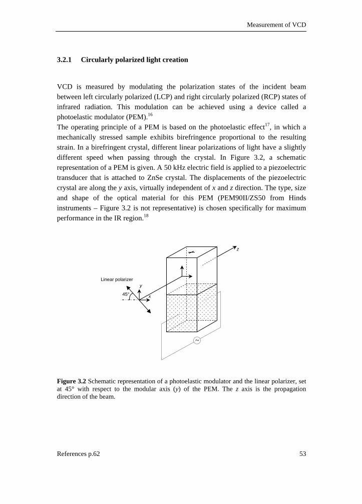
Measurement of VCD
References p.62 53
3.2.1 Circularly polarized light creation
VCD is measured by modulating the polarization states of the incident beam between left circularly polarized (LCP) and right circularly polarized (RCP) states of infrared radiation. This modulation can be achieved using a device called a photoelastic modulator (PEM).16 The operating principle of a PEM is based on the photoelastic effect17, in which a mechanically stressed sample exhibits birefringence proportional to the resulting strain. In a birefringent crystal, different linear polarizations of light have a slightly different speed when passing through the crystal. In Figure 3.2, a schematic representation of a PEM is given. A 50 kHz electric field is applied to a piezoelectric transducer that is attached to ZnSe crystal. The displacements of the piezoelectric crystal are along the y axis, virtually independent of x and z direction. The type, size and shape of the optical material for this PEM (PEM90II/ZS50 from Hinds instruments – Figure 3.2 is not representative) is chosen specifically for maximum performance in the IR region.18
Figure 3.2 Schematic representation of a photoelastic modulator and the linear polarizer, set at 45° with respect to the modular axis (y) of the PEM. The z axis is the propagation direction of the beam.
~
x
y
z
Linear polarizer
45°

Chapter 3
54
The electric field applied to the piezoelectric transducer, causes a sinusoidal stress modulation with frequency ωm = 50 kHz in the ZnSe crystal.19 Compression of the ZnSe crystal will induce a phase-lead of the y component, stretching will induce a phase lag.16 The maximal phase difference, and consequently, the maximum induced retardation δ0 is chosen to be π/2 (λ/4) at the centre of the aperture of the crystal. This means that the radiation with a specific frequency υi will be modulated between left and right circularly polarized light. This is shown in Figure 3.2, in which the phase difference is given as a function of time. In one period, the light will modulate from linearly polarized (LP) to LCP and RCP radiation, with intermediate elliptical polarization. Figure 3.4 the condition at maximum (RCP and LCP) and minimum (LP) instant phase difference are given. Here, the electric field vectors in x and y direction are given, and the resultant E following the path coordinate z of the light.
LP LPLP
LCP
δ 0= − π /2
δ 0= π /2RCP
δ
Figure 3.3 Phase difference δ versus time and the polarization states at several points in time with δ0=π/2. RCP = right circularly polarized, LCP = right circularly polarized and LP = linearly polarized

Measurement of VCD
References p.62 55
Figure 3.4 The condition of the x and y components of the electric field vectors at maximum (RCP and LCP) and minimum (LP) instant phase difference. z is the propagation direction of the radiation. 3.2.2 Signal detection
The beam that reaches the detector is doubly modulated. First, the light from the source is Fourier modulated. This low frequency modulated signal is then modulated between left and right circularly polarization states at a frequency of 50 kHz, which is significantly higher than the Fourier frequencies. The detector signal is pre-amplified and sent through a high- and low-pass filter. Passing the signal through a low-pass filter, as would be typically found in standard FTIR signal processing networks, yield a standard interferogram of the single beam transmission, often designated as the dc interferogram.20 This part of the detector signal is constant with respect to the polarization modulation.
Figure 3.5 The electronic block diagram for the PMA37 featuring the high-pass and low-pass channel.21
high-pass filter
low-pass filter
PEM ref.ωm
pre-amplifier
detector
multiplexer A/D
converter
RCP
LCP
LP
Ey
Ex
z
E
lock-in amplifier

Chapter 3
56
A 25 kHZ high-pass filter attenuates the Fourier modulated signals (low frequencies) in the detector signal, and is subsequently supplied to a lock-in amplifier (LIA) referenced to the PEM frequency. The intensity modulated signal at a frequency ωm generated by the VCD in the sample compartment, will be demodulated by the LIA. The output of the lock-in amplifier results in a signal from this VCD channel that is an interferogram corresponding to the polarization modulated signal alone,‡ often referenced to as the ac interferogram.20 The signals from both channels, i.e., the ac and dc interferograms, are subsequently multiplexed into a single channel and are fed to an analog-to-digital converter.21 The multiplexed interferogram can be processed using the macro provided by Bruker.21 When separated, the ac and dc interferograms are Fourier transformed, using the correct phase correction (see further), giving the ac and dc spectral intensities ( )acI ν and ( )dcI ν at the detector.23 The absorbance spectrum can be calculated from these intensities using Equation (3.1) with 0( )I ν the intensity at the detector in the absence of a sample.24
0
( )( ) log
( )dcI
AI
νν
ν= − (3.1)
For the differential absorbance spectrum, the relation in Equation (3.2) was derived,3 which is discussed extensively by Polavarapu.19
01
( )0.8686( )
( )2 ( )i
ac
dc
IA
IJ υ
νν
νδΔ = (3.2)
In the above equation 0
1( )i
J υδ is the first order Bessel function,25 0iυδ is the maximum
retardation induced by the PEM at frequency iν . It should be realized that the gain factors introduced by the electronics of the LIA and filters are not explicitly given in Equation (3.2) and should also be taken into account.19
‡ In References 19 and 22 an additional dc signal at the output of the LIA is mentioned which is attenuated with an additional low-pass filter. Such a filter is not documented for the PMA37 module.
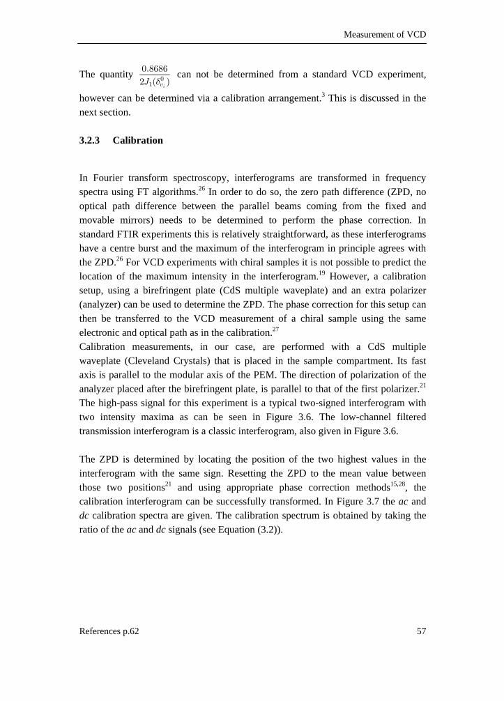
Measurement of VCD
References p.62 57
The quantity 01
0.86862 ( )
iJ υδ
can not be determined from a standard VCD experiment,
however can be determined via a calibration arrangement.3 This is discussed in the next section. 3.2.3 Calibration
In Fourier transform spectroscopy, interferograms are transformed in frequency spectra using FT algorithms.26 In order to do so, the zero path difference (ZPD, no optical path difference between the parallel beams coming from the fixed and movable mirrors) needs to be determined to perform the phase correction. In standard FTIR experiments this is relatively straightforward, as these interferograms have a centre burst and the maximum of the interferogram in principle agrees with the ZPD.26 For VCD experiments with chiral samples it is not possible to predict the location of the maximum intensity in the interferogram.19 However, a calibration setup, using a birefringent plate (CdS multiple waveplate) and an extra polarizer (analyzer) can be used to determine the ZPD. The phase correction for this setup can then be transferred to the VCD measurement of a chiral sample using the same electronic and optical path as in the calibration.27 Calibration measurements, in our case, are performed with a CdS multiple waveplate (Cleveland Crystals) that is placed in the sample compartment. Its fast axis is parallel to the modular axis of the PEM. The direction of polarization of the analyzer placed after the birefringent plate, is parallel to that of the first polarizer.21 The high-pass signal for this experiment is a typical two-signed interferogram with two intensity maxima as can be seen in Figure 3.6. The low-channel filtered transmission interferogram is a classic interferogram, also given in Figure 3.6. The ZPD is determined by locating the position of the two highest values in the interferogram with the same sign. Resetting the ZPD to the mean value between those two positions21 and using appropriate phase correction methods15,28, the calibration interferogram can be successfully transformed. In Figure 3.7 the ac and dc calibration spectra are given. The calibration spectrum is obtained by taking the ratio of the ac and dc signals (see Equation (3.2)).
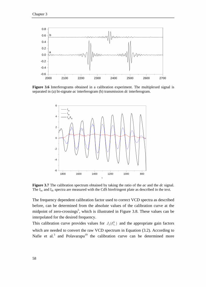
Chapter 3
58
2000 2100 2200 2300 2400 2500 2600 2700-0.6
-0.4
-0.2
0.0
0.2
0.4
0.6
0.8
b
a
Figure 3.6 Interferograms obtained in a calibration experiment. The multiplexed signal is separated in (a) bi-signate ac interferogram (b) transmission dc interferogram.
1800 1600 1400 1200 1000 800-6
-4
-2
0
2
4
6 Iac
Idc
Iac/Idc
ν Figure 3.7 The calibration spectrum obtained by taking the ratio of the ac and the dc signal. The Iac and Idc spectra are measured with the CdS birefringent plate as described in the text. The frequency dependent calibration factor used to correct VCD spectra as described before, can be determined from the absolute values of the calibration curve at the midpoint of zero-crossings5, which is illustrated in Figure 3.8. These values can be interpolated for the desired frequency. This calibration curve provides values for 0
1( )i
J υδ and the appropriate gain factors
which are needed to convert the raw VCD spectrum in Equation (3.2). According to Nafie et al.3 and Polavarapu19 the calibration curve can be determined more

Measurement of VCD
References p.62 59
accurately by performing a second calibration experiment in which the polarization direction is perpendicular to that of the first polarizer, and the fast axis of the birefringent CdS plate is perpendicular to the modular axis of the PEM crystal.
1800 1600 1400 1200 10000
1
2
3
4
5
6
ν Figure 3.8 Calibration spectrum from Figure 3.6 in which all values are taken positive. The calibration curve is determined by taking the midpoint at in the interval of zero crossings. 3.3 Experimental procedure
Compared to the situation thirty years ago, the measurement of VCD has evolved, and high-quality VCD spectra can be obtained fairly easy these days. Measurements can still be complicated due to the various problems that can occur, i.e., the presence of baseline artifacts29,30, weak VCD signal, low S/N ratios, etc. Baseline artifacts typically arise from strain in the lenses and windows through which the beam passes. The strain manifests itself as linear birefringence, which in turn alters the polarization state of the radiation as it passes through the components of the spectrometer.24 For our setup specifically, it was found that large baseline artifacts were induced at the detector. When the detector focus-lens was perfectly aligned giving a maximum signal at the detector, large artifacts were seen through a non-flat baseline. Reducing the signal at the detector by 10–15%, by moving the lens away from the detector, a much better baseline could be obtained. Cell windows

Chapter 3
60
also introduce baseline deviations, mainly due to strain effects of the windows (CaF2 and KBr). This was minimized by choosing the optimal orientation of the cell windows. In addition, artifacts can be associated with the absorbance characteristics of the sample24; if the absorbance due to the chiral sample or the applied solvent is too high, a poor S/N ratio is achieved. An absorbance of the solution between 0.7–1.0 absorbance units, which agrees with a transmittance between approximately 10% and 30%, is found to give an optimal S/N ratio. If the largest part of this absorption is attributable to the solvent, then the effective amount of light absorbed by the chiral sample is less, which gives also a poor S/N ratio. The presence of intense solvent absorption in regions of interest is therefore unfavorable. Solvents that were found useful in the 1800–800 cm−1 region are CDCl3, CD2Cl2, Cl2C=CCl2, and CS2. Path lengths were most often chosen in the range of 100 and 200 µm, using demountable cells with KBr and CaF2 windows. The optical filter placed before the first polarizer is a long wave pass filter with an operational frequency window between 1830 and 800 cm−1. This filter induces large artifacts near 1800 cm−1 which is unfavorable for investigations in this area, e.g. for the study of carbonyl stretch regions (see Chapter 8). In this frequency region a 1960 cm−1 limiting filter was therefore applied (Spectrogon, Sweden). The disadvantage of this filter is its relative small frequency window, as the long wave cutoff is at 1250 cm−1. As a result, in order to measure the VCD of a sample in the region between 1850 and 800 cm−1 two different filters were used. Various procedures can be found in the literature to facilitate the baseline (artifact) correction.8,19,24 An overview of such methods is given in Polavarapu et al.19,31 Recently, Nafie published24 a paper in which it is stated that the linear birefringence can be eliminated by introducing a second PEM. This was also claimed in a patent filed by BioTools in 2001 describing a prototype of this spectrometer.23 In this work, the baseline correction is performed applying various methods. The general idea is to obtain a background VCD that could be used as a baseline. To acquire such a background, ideally, a racemic mixture can be used (a 1:1 mixture of both enantiomers). Such a mixture is not optically active and will therefore exhibit no VCD. In principle, the racemic VCD spectrum will give a good estimate for the baseline.

Measurement of VCD
References p.62 61
If the racemic mixture is not available, one can measure the VCD for both enantiomers. The sum of their VCD divided by two, in principle gives the same baseline as one would obtain when measuring the racemic mixture, because the VCD artifacts for both enantiomers are the equal, that is, if the same optical and electronic path is followed. In the same manner, a baseline corrected VCD spectrum can be obtained for a specific enantiomer, by subtracting the VCD of the other enantiomer and divide the resulting spectrum by two. These spectra are often called half-sum and half-difference spectra.32 When the racemate and both enantiomers are not readily available, the baseline can be estimated via the measurement of the solvent VCD in the same conditions as the chiral sample. Because the absorbance artifacts for the solvent and the chiral compound are different, this method only gives an approximate baseline. However, in many cases, the baselines obtained via this method yield high quality spectra (see Chapters 6 and 8).33
Chapter 3
62
3.4 Reference list
1. Holzwart, G.; Hsu, E. C.; Mosher, H. S.; Faulkner, T. R.; Moscowit, A. J. Am.
Chem. Soc. 1974, 96, 251-252.
2. Hsu, E. C.; Holzwart, G. J. Chem. Phys. 1973, 59, 4678-4685.
3. Nafie, L. A.; Keiderling, T. A.; Stephens, P. J. J. Am. Chem. Soc. 1976, 98, 2715-2723.
4. Nafie, L. A.; Cheng, J. C.; Stephens, P. J. J. Am. Chem. Soc. 1975, 97, 3842-3843.
5. Keiderling, T. A. Vibrational Circular Dichroism. Comparison of Techniques and Practical Considerations. In Practical Fourier Transform Infrared Spectroscopy. Industrial and Laboratory Chemical Analysis., Ferraro, J. R., Krishnan, K., Eds.; Academic Press: San Diego, 1990; pp 203-284.
6. Su, C. N.; Heintz, V. J.; Keiderling, T. A. Chem. Phys. Lett. 1980, 73, 157-159.
7. Setnicka, V.; Urbanova, M.; Bour, P.; Kral, V.; Volka, K. J. Phys. Chem. A 2001, 105, 8931-8938.
8. Lipp, E. D.; Nafie, L. A. Appl. Spectrosc. 1984, 38, 20-26.
9. Lipp, E. D.; Zimba, C. G.; Nafie, L. A. Chem. Phys. Lett. 1982, 90, 1-5.
10. Nafie, L. A.; Diem, M. Appl. Spectrosc. 1979, 33, 130-135.
11. Nafie, L. A.; Diem, M.; Vidrine, D. W. J. Am. Chem. Soc. 1979, 101, 496-498.
12. Miyazawa, M.; Inouye, K.; Hayakawa, T.; Kyogoku, Y.; Sugeta, H. Appl. Spectrosc. 1996, 50, 644-648.
13. Hilario, J.; Drapcho, D.; Curbelo, R.; Keiderling, T. A. Appl. Spectrosc. 2001, 55, 1435-1447.
14. Wang, B. L.; Keiderling, T. A. Appl. Spectrosc. 1995, 49, 1347-1355.
15. Urbanova, M.; Setnicka, V.; Volka, K. Chirality 2000, 12, 199-203.
16. Hipps, K. W.; Crosby, G. A. J. Phys. Chem.-US 1979, 83, 555-562.

Measurement of VCD
63
17. Brewster, D. Philos. Trans. 1816, 106, 156.
18. Drake, A. F. J. Phys.-E-Sci. Instrum. 1986, 19, 170-181.
19. Polavarapu, P. L. Fourier transform infrared vibrational circular dichroism. In Fourier Transform Infrared Spectroscopy, Vol 4, Ferraro, J. R., Basile, L. J., Eds.; Academic Press, Inc.: Orlando, 1985; pp 61-95.
20. Nafie, L. A. Annu. Rev. Phys. Chem. 1997, 48, 357-386.
21. PMA 37 User's manual; Bruker: 2001.
22. Tsankov, D.; Eggimann, T.; Wieser, H. Appl. Spectrosc. 1995, 49, 132-138.
23. Nafie, L. A. US 6480277, 2002.
24. Nafie, L. A. Appl. Spectrosc. 2000, 54, 1634-1645.
25. Margenay, H.; Murphy, G. M. The mathematics of physics and chemistry; 2nd ed.; D. Van Nostrand Company, Inc.: New York, 1956; Vol. 1.
26. Griffiths, P. R. Chemical Infrared Fourier Transform Spectroscopy; 1st ed.; John Wiley & Sons: New York, 1975; Vol. 43.
27. Polavarapu, P. L. Appl. Spectrosc. 1984, 38, 26-28.
28. Mccoy, C. A.; Dehaseth, J. A. Appl. Spectrosc. 1988, 42, 336-341.
29. Cheng, J. C.; Nafie, L. A.; Stephens, P. J. J. Opt. Soc. Am. 1975, 65, 1031-1035.
30. Nafie, L. A.; Vidrine, D. W. Double Modulation Fourier Transform Spectroscopy. In Fourier Transform Infrared Spectroscopy: Applications to Chemical Systems, Ferraro, J. R., Krishnan, K., Eds.; Academic Press: New York, 1981; pp 83-123.
31. Polavarapu, P. L.; Michalska, D. F.; Back, D. M. Appl. Spectrosc. 1984, 38, 438-442.
32. Aamouche, A.; Devlin, F. J.; Stephens, P. J.; Drabowicz, J.; Bujnicki, B.; Mikolajczyk, M. Chem.-Eur. J. 2000, 6, 4479-4486.
33. Kuppens, T.; Herrebout, W.; van der Veken, B. J.; Corens, D.; De Groot, A.; Doyon, A.; Van Lommen, G.; Bultinck, P. Chirality 2006, 18, 609-620.

References p.80 65
4 comparison of spectra
Equation Chapter 4 Section 1 4.1 Introduction
An important part in the process of determining absolute configurations (AC) or predominant conformations using vibrational circular dichroism (VCD), is the comparison of the experimental and calculated spectra. Based on their agreement, that is, the location, sign and intensity of the bands, the AC can be assigned.1 However, experiments are inherently different compared to results that come from standard DFT calculations. Experimental spectra are recorded for dilute solutions, preferably non-polar solvents, to minimize the solvent-solute interaction (not to mention solute-solute interaction). Theoretical spectra are most often based on a single molecule in vacuum. Computed vibrational frequencies are also overestimated because of the harmonic approximation and the finite basis sets applied. Due to these differences in approach, “human eye” comparison is often a very subjective approach and can be biased by personal interpretation or as stated by W.C. Herndon and S.H. Bertz “Similarity, like beauty, lies in the eyes of the beholder”.2 In order to avoid such a bias, numerical comparisons should be performed. In this chapter, two different methods are discussed to compare and assess the agreement between experimental and calculated spectra; the classical, but labor

Chapter 4
66
intensive approach, in which the experimental bands are assigned to the calculated fundamental frequencies, and a new method, that applies similarity measures for the comparison. 4.2 Simulation of spectra
The calculation of dipole and rotational strengths and their corresponding vibrational frequencies allows the simulation of vibrational spectra for specific chiral compounds with known stereochemistry. For each significant conformation, single conformational spectra can be obtained. Line broadening can be introduced by assuming a Lorentzian band shape3,
2 21
( )( )i
if
αν
π ν ν α=
− + (4.1)
The band is centered at the frequency υi, and α is the Lorentzian half width at half max (hwhm). The full width at half max (fwhm) is defined as 2α. The area under the band is normalized due to the factor π−1. In Figure 4.1 a Lorentzian band is depicted, centered at υi = 0 cm−1 and α = 5 cm−1.
-30 -25 -20 -15 -10 -5 0 5 10 15 20 25 300.00
0.01
0.02
0.03
0.04
0.05
0.06
0.07
α
ν
f0(ν )
α
Figure 4.1 Lorentzian function f 0(υ) with a half width at half max (α) of 5 cm−1, υ is in cm−1.

Comparison of spectra
References p.80 67
The broadened single conformational spectra can be created and subsequently converted into molar absorptivity units based on Equations (2.6) and (2.13),
391
( ) ( )9 184 10 i i
i
D f.
ε ν ν ν−=⋅ ∑ (4.2)
391
( ) ( )2 296 10 i i
i
R f.
ε ν ν ν−Δ =⋅ ∑ (4.3)
Each single conformational spectrum can be taken into account using Boltzmann statistics, creating the simulated IR and VCD spectrum for the studied compound. These simulated spectra are actually produced to visualize the calculated data and to mimic the experimental spectra. This allows low-level comparison of experimental and theoretical spectra. Agreement between experimental and theoretical IR and VCD spectra allows the determination of the AC of the experimental sample. However, simple comparison, by superimposing both spectra, is not sufficient to determine ACs. A more thorough analysis of the available data has to be performed. One can correlate the experimental and the simulated/calculated bands based on the available IR and VCD data. Deconvolution of the experimental spectra allows the assessment of the experimental dipole and rotational strengths. Based on the assignment of the experimental bands the experimental and the theoretical dipole and rotational strengths can be compared. This approach is discussed in more detail in §4.3. Because this method is particularly labor-intensive, new tools were developed that allow the assessment of the similarity between experimental and theoretical spectra on the basis of a similarity measure. This measure quantifies the agreement between the two spectra giving fast and relatively accurate results. This is discussed in §4.4. 4.3 Assignment of fundamentals
To unambiguously assess the agreement between two spectra, a thorough analysis has to be performed. A reliable approach is the correlation of experimental and simulated bands. As VCD is a differential form of IR spectroscopy, IR and VCD transition frequencies are the same. Because of the differential intensities, VCD spectra have extra discriminating potential. As a result, assignment of unresolved IR
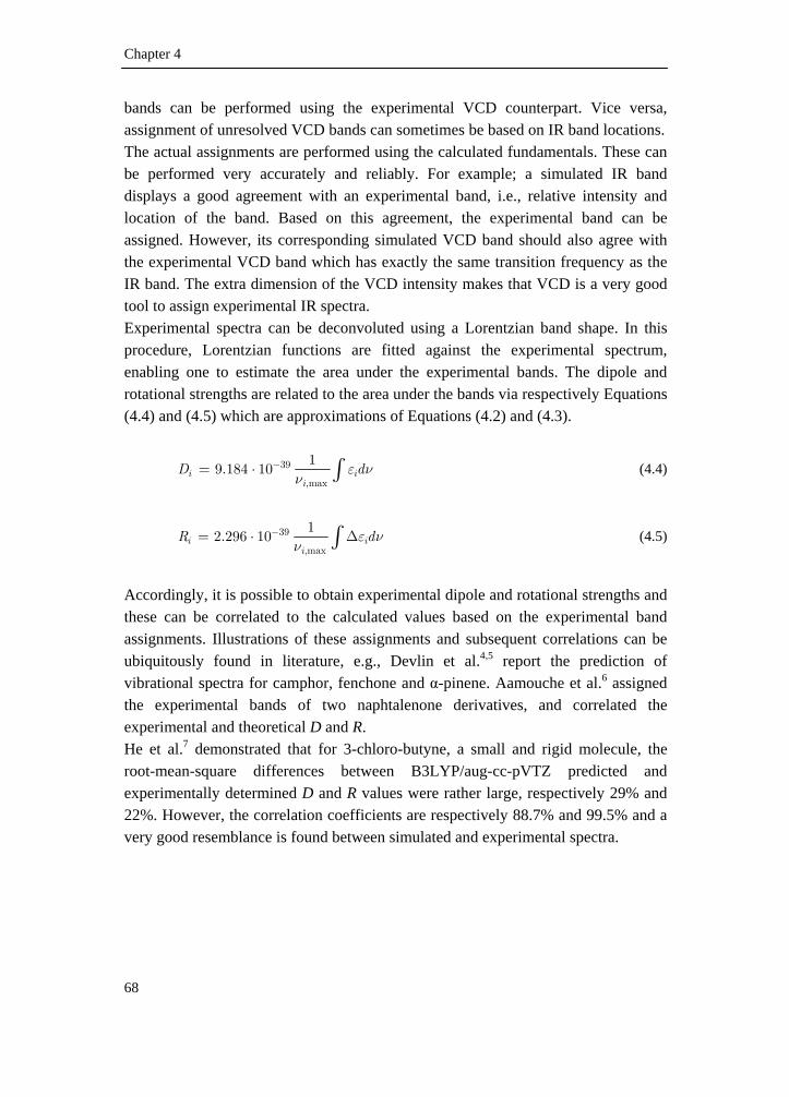
Chapter 4
68
bands can be performed using the experimental VCD counterpart. Vice versa, assignment of unresolved VCD bands can sometimes be based on IR band locations. The actual assignments are performed using the calculated fundamentals. These can be performed very accurately and reliably. For example; a simulated IR band displays a good agreement with an experimental band, i.e., relative intensity and location of the band. Based on this agreement, the experimental band can be assigned. However, its corresponding simulated VCD band should also agree with the experimental VCD band which has exactly the same transition frequency as the IR band. The extra dimension of the VCD intensity makes that VCD is a very good tool to assign experimental IR spectra. Experimental spectra can be deconvoluted using a Lorentzian band shape. In this procedure, Lorentzian functions are fitted against the experimental spectrum, enabling one to estimate the area under the experimental bands. The dipole and rotational strengths are related to the area under the bands via respectively Equations (4.4) and (4.5) which are approximations of Equations (4.2) and (4.3).
39
,max
19.184 10i i
iD dε ν
ν−= ⋅ ∫ (4.4)
39
,max
12.296 10i i
iR dε ν
ν−= ⋅ Δ∫ (4.5)
Accordingly, it is possible to obtain experimental dipole and rotational strengths and these can be correlated to the calculated values based on the experimental band assignments. Illustrations of these assignments and subsequent correlations can be ubiquitously found in literature, e.g., Devlin et al.4,5 report the prediction of vibrational spectra for camphor, fenchone and α-pinene. Aamouche et al.6 assigned the experimental bands of two naphtalenone derivatives, and correlated the experimental and theoretical D and R. He et al.7 demonstrated that for 3-chloro-butyne, a small and rigid molecule, the root-mean-square differences between B3LYP/aug-cc-pVTZ predicted and experimentally determined D and R values were rather large, respectively 29% and 22%. However, the correlation coefficients are respectively 88.7% and 99.5% and a very good resemblance is found between simulated and experimental spectra.

Comparison of spectra
References p.80 69
In this work, correlation between experimental/theoretical dipole and rotational strengths is performed for most studied compounds, i.e., in Chapters 5, 6, 7 and §8.4. 4.4 Spectral comparison
In this section, the concepts of correlation functions and similarity measures are proposed for the purpose of spectral comparison. 4.4.1 Correlation functions
The function that describes the overlap of two patterns as a function of a relative shift r, is called a correlation function. If we define two functions f(x) and g(x), the auto-correlation function can be written as,
( ) ( ) ( )ffc r f x f x r dx= +∫ (4.6)
and the cross-correlation function,
( ) ( ) ( )fgc r f x g x r dx= +∫ (4.7)
The integral of cff(r), the auto-correlation integral, is given by
( )2( ) ( )ffc r dr f x dx=∫ ∫ (4.8)
The cross-correlation integral is similarly written as
( ) ( ) ( )fgc r dr f x dx g x dx=∫ ∫ ∫ (4.9)
From Equation (4.9) it can be seen that the area under the cross-correlation function is always equal to the product of the areas under the patterns f(x) and g(x). The cross-correlation function can therefore be normalized by dividing it by the root of
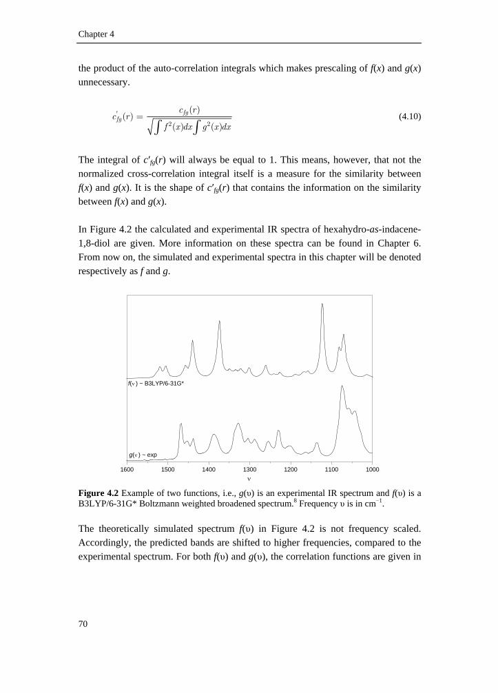
Chapter 4
70
the product of the auto-correlation integrals which makes prescaling of f(x) and g(x) unnecessary.
'
2 2
( )( )
( ) ( )
fgfg
c rc r
f x dx g x dx=
∫ ∫ (4.10)
The integral of c′fg(r) will always be equal to 1. This means, however, that not the normalized cross-correlation integral itself is a measure for the similarity between f(x) and g(x). It is the shape of c′fg(r) that contains the information on the similarity between f(x) and g(x). In Figure 4.2 the calculated and experimental IR spectra of hexahydro-as-indacene-1,8-diol are given. More information on these spectra can be found in Chapter 6. From now on, the simulated and experimental spectra in this chapter will be denoted respectively as f and g.
1600 1500 1400 1300 1200 1100 1000
f(ν ) ~ B3LYP/6-31G*
ν
g(ν ) ~ exp
Figure 4.2 Example of two functions, i.e., g(υ) is an experimental IR spectrum and f(υ) is a B3LYP/6-31G* Boltzmann weighted broadened spectrum.8 Frequency υ is in cm−1. The theoretically simulated spectrum f(υ) in Figure 4.2 is not frequency scaled. Accordingly, the predicted bands are shifted to higher frequencies, compared to the experimental spectrum. For both f(υ) and g(υ), the correlation functions are given in

Comparison of spectra
References p.80 71
Figure 4.3. The area under the correlation functions is normalized. The different shapes of the curves give information on the agreement between f(υ) and g(υ).
-600 -400 -200 0 200 400 6000.000
0.001
0.002
0.003
0.004
c'ff(r)
r
c'gg(r)
c'fg(r)
Figure 4.3 Normalized auto-correlation c′ff(r) and c′gg(r) and cross-correlation c′fg(r) functions for f(ν) and g(ν) as given in Figure 4.2. The relative shift r is given in cm−1. The maxima of the auto-correlation functions are situated at a relative shift r = 0. The cross-correlation function has a maximum at r = 48 cm−1, which indicates that, if the frequencies of g(υ) are shifted over 48 cm−1, the largest similarity can be found. In contrast to IR spectra, a function that represents a VCD spectrum can have negative function values. Correlation functions of non-positive functions can not always be defined. For example, the normalized auto-correlation function of a sine function in the interval [−π, π] is infinite because the normalization factor
2
sinxdxπ
π
−
−
⎡ ⎤⎢ ⎥⎢ ⎥⎢ ⎥⎣ ⎦∫ is zero.
If, for a non-positive function, the positive and negative parts are dealt with separately, the evaluation of the correlation functions can be performed. The non-positive function is split-up into two functions, which then both can be evaluated as positive functions.

Chapter 4
72
In Figure 4.4, the experimental and simulated VCD spectra are given, again for hexahydro-as-indacene-1,8-diol. Both spectra are partitioned, separating the negative and positive function values. f +(υ) and g+(υ) are formed by substituting all negative values with zero function values. f −(υ) and g−(υ) are formed similar for the negative part.
1600 1500 1400 1300 1200 1100 1000
ν
g(ν ) ~ exp
f(ν ) ~ B3LYP/6-31G*
Figure 4.4 Example of two functions, i.e., g(υ) is an experimental VCD spectrum and f(υ) is a B3LYP/6-31G* Boltzmann weighted broadened spectrum.8 Both spectra are partitioned, i.e., f +(υ) and g+(υ) (black) and f −(υ) and g−(υ) (red) separating positive and negative function values. υ is in cm−1. These positive and negative functions can separately be evaluated yielding positive and negative correlation function (c+ and c−) and are given in Figure 4.5. In Figure 4.5 it can be seen that the maxima in the positive and negative cross-correlation functions are respectively shifted towards r values of approximately 32 and 70 cm−1. The higher value for the negative cross-correlation function is due to the large deviation between the positive predicted rotational strength and the negative observed band for fundamental 37 and is discussed in more detail in Chapter 6.

Comparison of spectra
References p.80 73
-600 -400 -200 0 200 400 6000.0000.0010.0020.0030.0040.0050.0060.0070.0080.0090.010
c+'ff(r)
r
c+'gg(r)
c+'fg(r)
-600 -400 -200 0 200 400 6000.0000.0010.0020.0030.0040.0050.0060.0070.0080.009
c-'ff(r)
r
c-'gg(r)
c-'fg(r)
Figure 4.5 Top: Normalized auto-correlation c+′ff(r) and c+′gg(r) and cross-correlation c+′fg(r) functions for f +(υ) and g+(υ) as given in Figure 4.4. Bottom: Normalized auto-correlation c−′ff(r) and c−′gg(r) and cross-correlation c−′fg(r) functions for f −(υ) and g−(υ) as given in Figure 4.4. The relative shift r is given in cm−1. It is clear now that the similarity information for two spectra is embedded in the shape of the cross-correlation function. By using a special window function, this information can be extracted.
Chapter 4
74
4.4.2 Generalized expression for similarity
In the previous section, it was described that the normalized cross-correlation integral does not contain any information on the similarity of two spectra. If one introduces a weighting function, the interval for the local shift can be chosen. Accordingly, a generalized expression9 for the similarity S between f(x) and g(x), can be written,
( ) ( )
( ) ( ) ( ) ( )
fg fg
ff ff gg gg
w r c r drS
w r c r dr w r c r dr=
∫∫ ∫
(4.11)
The weighting function ( )fgw r determines in which manner the similarity
information is extracted from the cross-correlation function. ( )ffw r and
( ) ggw r determine the normalization of the weighted cross-correlation function via
the auto-correlation functions. A normalized similarity measure is only obtained if the following conditions hold: ( )= ( )= ( ) ff fg ggw r w r w r (4.12)
If the weighting function is chosen as
( ) 1 0
( ) 0 0
w r if r
w r if r
= =
= ≠ (4.13)
the similarity measure in Equation (4.11) is reduced to the overlap integral of both functions, i.e., no relative shift is introduced. To include the neighborhood in the comparison of the spectra, the weighting function should be defined for r ≠ 0. Karfunkel et al.10 proposed their fold criterion, using the function (4.14) which is depicted in Figure 4.6.
1( )
1w r
r βα=
+ (4.14)

Comparison of spectra
References p.80 75
A triangular function9 as presented in Equation (4.15) and in Figure 4.6 can also be used as a weighting function.
( ) 1
( ) 0
rw r if r l
lw r if r l
= − <
= ≥ (4.15)
-20 -10 0 10 20
0
1
Fold: α =103,β =4 triangle: l = 4 cm-1
triangle: l = 14 cm-1
r
w(r)
Figure 4.6 Representation of different weighting functions; fold criterion (α = 103 and β = 4), and triangular functions (l = 4 and 14 cm−1). The variable r is in cm−1. Next to the local shifting of function g(x), one can also introduce a scaling factor σ into the function f(x), which could be interesting for the comparison of vibrational spectra. The correlation function (4.7) is accordingly written,
( ) ( ) ( )fgc r f x g x r dxσ σ= +∫ (4.16)
The similarity expression in (4.11) can be rewritten using scaled correlation functions as defined in (4.16), which gives the scaled similarity Sσ,
( ) ( )
( ) ( ) ( ) ( )
fg fg
ff ff gg gg
w r c r drS
w r c r dr w r c r dr
σσ
σ σ=
∫∫ ∫
(4.17)

Chapter 4
76
When the weighting functions are chosen as defined in (4.13), i.e., only considering the correlation function at r = 0, the similarity measure in (4.17) reduces to a scaled overlap measure,
2 2
( ) ( )
( ) ( )
f x g x dxS
f x dx g x dx
σσ
σ=
∫∫ ∫
(4.18)
In Chapter 5, this measure is used to describe the similarity between theoretical and experimental spectra and the mutual agreement between theoretical spectra. In the next section the introduced triangular function will be used to define a similarity measure that takes into account neighborhoods. 4.4.3 Neighborhood similarity
When calculating vibrational frequencies using ab initio methods, usually a harmonic potential is applied to describe nuclear vibrational motion. In combination with finite basis sets, the predicted frequencies are overestimated. It is common use to correct for this overestimation by scaling the frequencies with a uniform factor. This scaling depends on the applied method and basis set.11,12 Evidently, it is important to take this scaling into consideration when comparing the experimental and simulated spectra. The similarity measure in Equation (4.17) introduces a scaling factor σ that allows the correction for the overestimated calculated frequencies. Linear scaling is far from perfect, as simulated bands can still be shifted with respect to their corresponding experimental bands. A good similarity measure should therefore take into account the neighborhood in direct proximity of the bands. If, in Equation (4.17), a triangular shaped weighting function as defined in Equation (4.15) is chosen, neighborhood comparison can be performed. The fold criterion is not used, because the implementation of this function is more complex due to the parameters α and β. These have no intuitive meaning in contrast to the parameter l in the triangular weighting function. l (in cm−1) defines the interval for which the relative shift is taken into account. A triangular function is also easy to implement and is was shown that these functions give stable results for XRD spectral comparison.9

Comparison of spectra
References p.80 77
In Figure 4.7, the experimental and simulated IR spectra (1500–1325 cm−1 interval) for di-epoxy-as-indacene is given. The corresponding bands are labeled based on the fundamental assignment (see Chapter 6). The frequencies of f(ν) are not scaled, which can clearly be seen in Figure 4.7. Evaluation of the spectral similarity using the scaled overlap defined in Equation (4.18) yields a value of 66.8% for an optimal scaling factor σ = 0.954. It can be observed that band 52/51 is shifted relative to the two other labeled bands. The spectral similarity assessment can only be effective when this effect is taken into account considering the neighborhoods of the bands. Using the triangular weight function with a windows size l = 40 cm−1, the neighborhood similarity expression in Equation (4.17) yields a value of 94.0% with σopt = 0.957. The latter is clearly a better quantification for the similarity of both spectra compared to the scaled overlap measure.
1550 1500 1450 1400 1350
49
50
52/5
1
52/5
1
54/5
3
g(ν )
ν
50/4
9
f(ν )
54/5
3
Figure 4.7 1500–1325 cm−1 part of the experimental and B3LYP/6-31G* simulated (frequencies are not scaled) IR spectra for di-epoxy-as-indacene (Chapter 6). Bands are numbered based on calculated fundamentals. The size and the shape of the window/weighting function is chosen based on the observation that corresponding bands can be shifted towards each other, but only locally. If they are shifted more than 40 cm−1, after scaling, it is unlikely that these bands are correlated. The calculation of neighborhood similarities for VCD spectra, is somewhat more complicated because the positive and negative part of the spectrum need to be evaluated separately. Using the positive and negative correlation functions that were

Chapter 4
78
defined previously, two similarity expressions can be written, i.e., ,S σ + and ,S σ − . The neighborhood similarity measure S σ for VCD spectra is then defined as the arithmetic mean of ,S σ + and ,S σ − ,
, ,
2S S
Sσ σ
σ+ −+
= (4.19)
4.4.4 Numerical integration
The calculation of the neighborhood similarity using a triangular window function is implemented using Fortran. To evaluate correlation functions and correlation integrals for discrete functions, that is, sampled spectra, numerical integration methods are needed. IR and VCD spectra are a set of two dimensional points, for which an intensity is specified for certain discrete wavenumbers/frequencies. The objective of numerical integration is to compute an approximate solution to the definite integral:
( )b
a
I f x dx= ∫ (4.20)
There are a wide range of methods available to perform numerical integration.13 For our purpose, Simpson’s rule is applied in combination with Richardson extrapolation.14 Our implementation was written in Fortran on the basis of the “Numerical Recipes in Fortran77” code14 which was altered for a better performance. The performance of the numerical integration routine is illustrated, using the product of two Gaussian functions. Gaussians are chosen here, because the product of two Gaussians has a well known analytical expression.15
2
2
( 10)1
( 11)2
x
x
f e
f e
− −
− −
=
= (4.21)
For this integral an analytical expression of the solution is known,
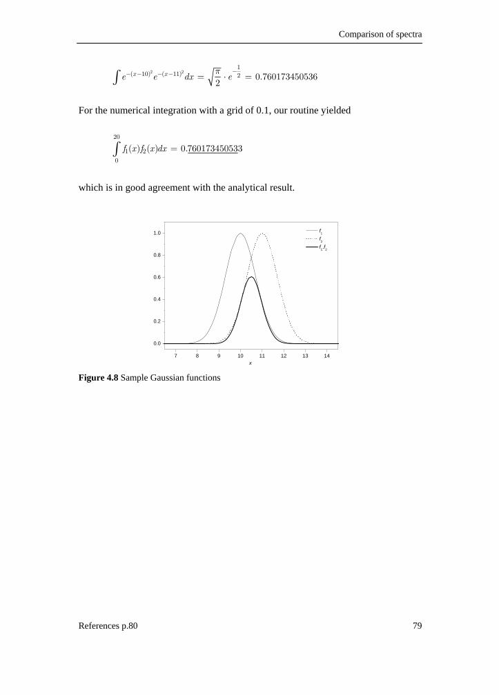
Comparison of spectra
References p.80 79
2 21
( 10) ( 11) 2 0.7601734505362
x xe e dx eπ −− − − − = ⋅ =∫
For the numerical integration with a grid of 0.1, our routine yielded
20
1 2
0
( ) ( ) 0.760173450533f x f x dx =∫
which is in good agreement with the analytical result.
7 8 9 10 11 12 13 14
0.0
0.2
0.4
0.6
0.8
1.0
f1 f
2
f1.f2
x Figure 4.8 Sample Gaussian functions
Chapter 4
80
4.5 Reference list
1. Freedman, T. B.; Cao, X. L.; Dukor, R. K.; Nafie, L. A. Chirality 2003, 15,
743-758.
2. Herndon, W. C.; Bertz, S. H. J. Comput. Chem. 1987, 8, 367-374.
3. Schellman, J. A. Chem. Rev. 1975, 75, 323-331.
4. Devlin, F. J.; Stephens, P. J.; Cheeseman, J. R.; Frisch, M. J. J. Phys. Chem. A 1997, 101, 6322-6333.
5. Devlin, F. J.; Stephens, P. J.; Cheeseman, J. R.; Frisch, M. J. J. Phys. Chem. A 1997, 101, 9912-9924.
6. Aamouche, A.; Devlin, F. J.; Stephens, P. J. J. Am. Chem. Soc. 2000, 122, 7358-7367.
7. He, J. T.; Petrovich, A.; Polavarapu, P. L. J. Phys. Chem. A 2004, 108, 1671-1680.
8. Kuppens, T.; Vandyck, K.; Van der Eycken, J.; Herrebout, W.; van der Veken, B. J.; Bultinck, P. J. Org. Chem. 2005, 70, 9103-9114.
9. De Gelder, R.; Wehrens, R.; Hageman, J. A. J. Comput. Chem. 2001, 22, 273-289.
10. Karfunkel, H. R.; Rohde, B.; Leusen, F. J. J.; Gdanitz, R. J.; Rihs, G. J. Comput. Chem. 1993, 14, 1125-1135.
11. Scott, A. P.; Radom, L. J. Phys. Chem.-US 1996, 100, 16502-16513.
12. Wong, M. W. Chem. Phys. Lett. 1996, 256, 391-399.
13. Davis, P. J.; Rabinowitz, P. Methods of Numerical Integration, New York: Academic Press, 1984.
14. Press, W. H.; Teukolsky, S. A.; Vetterling, W. T.; Flannery, B. P. Numerical Recipes in Fortran 77; 2nd ed.; Cambridge University Press: 1992.
15. Szabo, A.; Ostlund, N. S. Modern Quantum Chemistry; Dover Publications, Inc.: New York, 1996.
References p.108 81
5 determination of the
stereochemistry of hydroxymethyl
dihydrodioxinopyridine by VCD
and the effect of DFT integration
grids
Equation Chapter 5 Section 1 5.1 Introduction
It is well known that optical isomers may demonstrate a different biological activity.1 Therefore, in the pharmaceutical industry, the knowledge of the absolute configuration is of the utmost importance. Among several methods available to determine the absolute configuration, X-ray diffraction (XRD) is often the method of choice because it yields the most reliable results. This relatively labor-intensive method requires the availability of well-defined crystals and the presence of heavy atoms, which is often a problem. A second popular method, nuclear magnetic resonance (NMR), is not always applicable either. Often specific methods have to be Kuppens, T.; Langenaeker, W.; Tollenaere, J. P.; Bultinck, P. J. Phys. Chem. A 2003, 107, 542-553

Chapter 5
82
applied to eliminate the degeneracy of the enantiomers e.g., the use of chiral solvents or chiral shift-reagents. These methods are sometimes troublesome and may give contradictory results.2-4 Retro-synthesis also has several drawbacks, and is usually labor-intensive. A technique that holds great promise for the determination of the absolute configuration and gains importance quite rapidly, is the measurement of vibrational circular dichroism (VCD). This technique is based on the differential absorption of left and right circularly polarized infrared (IR) radiation. Because circularly polarized light (CPL) itself has handedness, different interactions of the two forms of light occur with chiral molecules, i.e., the differential CPL absorptions of two enantiomers are opposite in sign. For VCD to be applicable, the acquired spectra should be interpretable. However, interpretation of VCD spectra is not straightforward and it requires an algorithm that relates both the structure and spectra. Hence the necessity to predict spectra for different stereoisomers. By comparing the predicted spectrum with the experimental spectrum, identification of the stereoisomer present in solution is possible. The main issue in the calculation of the theoretical spectra is the sign of the differential transitions and the prediction of the rotational strength, which is proportional to the area of the VCD band. A reliable quantum chemical method for molecules of variable size was developed by Stephens et al. in 1996.5-8 Several studies have already illustrated the applicability of this method in determining the absolute configuration of a chiral molecule.9,10 From an experimental point of view, VCD exhibits several important advantages. Nowadays, VCD spectra can be measured almost routinely, using specially adapted IR spectrometers. An even more important advantage over XRD techniques is that measurements are possible in solvents, i.e., there is no need for crystals or “heavy” atoms. In this study, the absolute configuration of 3-hydroxymethyl-2,3-dihydro-[1,4]dioxino[2,3-b]pyridine, 1, shown in Figure 5.1 is known by its synthesis route.11 The R and S enantiomers respectively correspond to the samples with positive and negative optical rotation. VCD spectra have been recorded for the R and S enantiomer. Both spectra were made available to the authors of the present study without revealing any stereochemical information. DFT calculations were used to simulate VCD spectra for both the R and S enantiomer, and by comparison between the experimental and
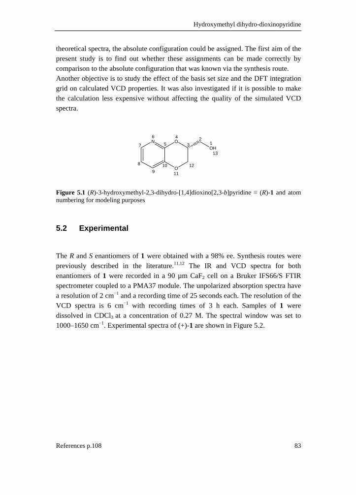
Hydroxymethyl dihydro-dioxinopyridine
References p.108 83
theoretical spectra, the absolute configuration could be assigned. The first aim of the present study is to find out whether these assignments can be made correctly by comparison to the absolute configuration that was known via the synthesis route. Another objective is to study the effect of the basis set size and the DFT integration grid on calculated VCD properties. It was also investigated if it is possible to make the calculation less expensive without affecting the quality of the simulated VCD spectra.
N
O
OOH1
23
45
6
7
8
910
11
12
13
Figure 5.1 (R)-3-hydroxymethyl-2,3-dihydro-[1,4]dioxino[2,3-b]pyridine ≡ (R)-1 and atom numbering for modeling purposes 5.2 Experimental
The R and S enantiomers of 1 were obtained with a 98% ee. Synthesis routes were previously described in the literature.11,12 The IR and VCD spectra for both enantiomers of 1 were recorded in a 90 µm CaF2 cell on a Bruker IFS66/S FTIR spectrometer coupled to a PMA37 module. The unpolarized absorption spectra have a resolution of 2 cm−1 and a recording time of 25 seconds each. The resolution of the VCD spectra is 6 cm−1 with recording times of 3 h each. Samples of 1 were dissolved in CDCl3 at a concentration of 0.27 M. The spectral window was set to 1000–1650 cm−1. Experimental spectra of (+)-1 are shown in Figure 5.2.

Chapter 5
84
Figure 5.2 IR (top) and VCD (bottom) spectra for (+)-1, including Lorentzian fit and error. Intensities and differential intensities are in molar absorptivity units, frequencies in cm−1.
-0.04
-0.03
-0.02
-0.01
0
0.01
0.02
0.03
0.04
10001050110011501200125013001350140014501500155016001650
Experiment
Lorentzian fit
Error
ν
Δε
0
100
200
300
400
500
600
700
800
900
10001050110011501200125013001350140014501500155016001650
experiment
lorentzian fit
error
ε
ν

Hydroxymethyl dihydro-dioxinopyridine
References p.108 85
5.3 Computational methodology
Multiple conformations of 1 are possible and each conformation contributes to the IR and VCD spectra of the molecule. Because calculated spectra depend heavily on the molecular conformation,13 a thorough conformational analysis is needed. To find the different minimum energy conformations of the molecule, a two-way conformational analysis approach is used. In the first approach, B3LYP/6-31G* calculations are used. The pyridine ring is considered rigid, whereas the dioxane ring, as well as all other fragments, are considered flexible. The dihedral angles are developed in a 60° grid. Not all resulting structures are chemically sound, and prior to initiating a geometry optimization the search tree is pruned by the application of a bump check and ring constraints. The remaining conformations are then optimized on the B3LYP/6-31G* level. The resulting minima are collected for further geometry optimizations and spectroscopic calculations. A major problem with systematic searches is the combinatorial explosion, which hampers systematic searches for larger molecules and finer dihedral angle grids. The computational requirements of DFT calculations are such that finer dihedral grids in a systematic search are not practicable.‡ Therefore a stochastic search was also applied using the MM3 force field.14 This method, as implemented in the MM3(96) program,15 optimizes the geometry of a molecule and randomly moves (kicks) each atom in an atom-centered sphere with a predefined radius. The new structure is then reoptimized, yielding a new or possibly previously located stationary point, after which the geometry of this new stationary point is again randomly kicked. Own routines are used to automate the entire search and check for convergence. The conformational search is considered converged if all minima with a relative energy – compared to the global minimum – below 20 kcal/mol are found more than 20 times and a new stochastic search does not yield any new minima.16 Redundant structures are also removed by compiling the lists of stationary points from different stochastic searches. DFT molecular geometries were obtained by the minimization of the MM3 geometries of the stationary points found during the MM3 conformational search. These were supplemented with the B3LYP/6-31G* geometries from the ab initio conformational analysis. DFT calculations are performed with Gaussian98 rev A617
‡ At that moment, i.e., 2002

Chapter 5
86
using the B3LYP hybrid density functional7,18,19 and DZ and TZ Pople style basis sets, i.e., 6-31G, 6-31G*, 6-31G** and 6-311G**.20 The cc-pVDZ, cc-pVTZ and cc-pVQZ Dunning basis sets are also applied. Default Gaussian98 basis set parameters are used. For the geometry optimization and the calculation of the spectroscopic properties different integration grids are applied. Euler-Maclaurin-Lebedev grids of the type (m,n) are used, having m radial shells and n angular points per shell. Pruned21 versions of these grids are also applied. In the latter the number of angular points varies with the shell with a maximum of n on radii that are relevant for chemical bonding.22 The default grid in Gaussian98 is a pruned version of the (75,302) grid further denoted as (75,302)p, invoked with the keyword GRID=FineGrid. The (50,194)p grid21 is invoked with the keyword GRID=SG1Grid and the (35,110)p grid with GRID=CoarseGrid.23 Other grids can be used by specifying the INT(GRID=mn) keyword. Gauge including/invariant atomic orbitals (GIAO) are used to calculate atomic axial tensors (AAT). Together with harmonic force fields and atomic polar tensors (APT) the rotational strengths are calculated.5-7 For each DFT energy minimum in the potential surface, the dipole and rotational strengths are calculated. The resulting line spectra are then broadened using a Lorentzian band shape giving single conformer spectra. For the total frequency range, the total broadened dipole and rotational strength is calculated as the weighted sum of the single conformer spectra (Equation (5.1)). In other words; the IR and VCD spectra of a molecule is computed as a linear combination of the spectra for the different conformations.
tot A
A
tot AA
( ) P(A) ( )
( ) P(A) ( )
D v D v
R v R v
= ⋅
= ⋅
∑
∑ (5.1)
P(A), being the population of conformer A, is calculated assuming a Boltzmann distribution (Equation (5.2)) where i runs over all conformers,
0A
0P(A)i
H RT
H RT
i
e
e
−
−=∑
(5.2)

Hydroxymethyl dihydro-dioxinopyridine
References p.108 87
We omit the entropic contributions to the Gibbs free energy and, consequently, use the enthalpy to calculate the conformational populations.24 The enthalpy is calculated via DFT using the standard thermochemical expressions and under the usual assumptions.25 A quantitative measure has to be introduced to discuss the similarity of spectra. We use a measure based on the overlap integral given in Equation (5.3),
2 2
( ) ( )
( ) ( )
f g dS
f d g d
σσν ν ν
σν ν ν ν=
∫∫ ∫
(5.3)
where f and g are the functions that represent the spectral intensities at each frequency ν. Identical spectra have an overlap integral equal to 1. For IR spectra, with no negative values, the overlap integral tends to 0 when the similarity becomes smaller. For VCD spectra however the overlap can become negative, and Sσ is equal to −1 when the spectra are the opposite of each other, that is, when both spectra are from enantiomers. Frequency scaling is introduced by the factor σ. Experimental IR and VCD spectra are Lorentzian fitted to calculate the experimental dipole and rotational strengths via following relations;26
39
39
9.184 10
2.296 10
i i
i i
dD
dR
νε
νν
εν
−
−
= ⋅
= ⋅ Δ
∫
∫ (5.4)
Here, ε and Δε are the absorptivity and differential molar absorptivity in l.mol−1cm−1. D and R are in esu2cm2.

Chapter 5
88
5.4 Results and discussion
5.4.1 Conformational analysis
Conformational isomers of 1 differ by :
- the orientation of the exocyclic bond (τ1, O11C12C3C2), i.e., pseudo-equatorial or pseudo-axial,
- the rotameric dihedral angle about the C2–C3 bond (τ2, O4C3C2O1) and - the rotameric dihedral angle about the O1–C2 bond (τ3, C3C2O1H13).
The position of the exocyclic substituent, that is, the methylhydroxyl group, is either designated as eq or ax. Assuming three typical minima in the torsion potential energy, that is, 60°, 180° and −60°, the dihedral angles are respectively denoted as gauche clockwise (G), trans (T) and gauche counterclockwise (G’) for the C–C bond torsion (τ2), and similarly g, t and g’ for the O–C bond torsion (τ3). The combined conformational search yielded 10 stationary points, all corresponding to minima on the MM3 PES. These are shown in Table 5.1 and Figure 5.3 with their corresponding notation, relative MM3 energies and corresponding values for τ1, τ2 and τ3. Table 5.1 MM3 minima, conformational description, relative MM3 energy (RE, in kcal/mol) and key dihedral angles (τ1, τ2 and τ3, in degrees).
RE
MM3 τ1
O11C12C3C2 τ2
O4C3C2O1 τ3
C3C2O1H13 1 eqGg’ 0.00 179 63 −54 2 eqG’g 0.08 178 −61 58 3 axGg’ 0.64 −59 61 −57 4 eqG’t 1.60 176 −68 170 5 eqTt 1.63 179 179 −177 6 eqGt 1.80 178 69 −172 7 axG’g 1.84 −67 −68 39 8 axGt 2.43 −59 69 −169 9 axTt 2.45 −60 177 179 10 axG’t 4.72 −67 −68 170

Hydroxymethyl dihydro-dioxinopyridine
References p.108 89
Figure 5.3 Visualization of the PES minima for (R)-1.

Chapter 5
90
All 10 minima were used as starting geometries for geometry optimizations using the B3LYP functional and the different basis sets mentioned above. These geometry optimizations were not straightforward. Through application of constrained geometry optimizations, we succeeded in locating most minima with the different Pople style basis sets. A common feature for these basis sets is the fact that no axG’t structure could be located. The 6-31G basis set was found to be severely lacking in giving a good description of the molecular PES. Given the conformational dependence of the VCD spectra, this basis set was not further considered. For the cc-pVDZ and cc-pVTZ basis set only conformations with a relative energy below 3 kcal/mol (according to 6-311G**) were minimized. A summary of the results of these different geometry optimizations is presented in Table 5.2. Table 5.2 B3LYP relative energies (in kcal/mol) for the located minima, the conformational description and MM3 energy ranking. For the cc-pVDZ and cc-pVTZ basis set only the 5 lowest energy conformations are considered.
6-31G* 6-31G** 6-311G** cc-pVDZ cc-pVTZ 2 eqG’g 0.00 0.00 0.00 0.00 0.00 1 eqGg’ 0.81 0.84 0.81 0.85 0.55 3 axGg’ 1.60 1.61 1.60 1.63 1.55 5 eqTt 2.49 2.49 2.06 2.56 1.78 9 axTt 2.94 2.91 2.52 2.90 2.40 4 eqG’t 3.59 3.54 3.21 - - 7 axG’g 4.28 4.30 4.14 - - 6 eqGt 4.96 4.92 4.47 - - 8 axGt 5.41 5.36 4.97 - -
Tables 5.1 and 5.2 clearly show that the relative energies of the different structures differ quite strongly between the MM3 and DFT levels of theory. The energetic ordering of the minima also undergoes a number of changes. Most notably, on the MM3 level, the structures with an equatorial exocyclic bond were lower in energy than those with an axial exocyclic bond (except for the axGg’ structure). On the DFT level there is no longer such a clear distinction between both types of structures. The relative energies found using the 6-31G* and 6-31G** basis sets differ little, but when going to the 6-311G** basis set, the energetic spread of the minima is reduced. This effect is also found when going from the cc-pVDZ to the cc-pVTZ basis set. As mentioned above, the 6-31G basis set yields fewer minima, and for those that were found, the relative energies differ strongly from the more extended basis sets (data not shown).

Hydroxymethyl dihydro-dioxinopyridine
References p.108 91
Table 5.3 MM3 ranking, conformational description, relative B3LYP/6-31G* energy (RE, in kcal/mol) and optimized key dihedral angles (τ1, τ2 and τ3, in degrees).
RE τ1
O11C12C3C2 τ2
O4C3C2O1 τ3
C3C2O1H13 2 eqG’g 0.00 −177.1 −60.4 58.0 1 eqGg’ 0.81 −178.4 58.1 −53.4 3 axGg’ 1.60 −64.1 56.1 −52.2 5 eqTt 2.49 −178.9 176.6 −178.7 9 axTt 2.94 −65.2 171.4 174.5 4 eqG’t 3.59 178.5 −74.3 163.2 7 axG’g 4.28 −69.7 −59.0 70.3 6 eqGt 4.96 179.6 73.2 −162.3 8 axGt 5.41 −63.5 68.4 −162.5
Table 5.3 gives the dihedral angles τ1, τ2 and τ3 for the optimized B3LYP/6-31G* geometries. The comparison with Table 5.1 clearly shows that the dihedral angles in the MM3 structures agree quite well with the DFT values. Table 5.4 gives the relative energies using various DFT integration grids. Only small distinctions between the different grids are found, with the exception of the (35,110)p grid. The extent of the difference between the (35,110)p grid and the other grids also depends on the conformations involved. Table 5.5 gives the energy difference (in µhartree) for the eqGg’ conformer relative to the (99,974) grid energy. Again, only minor effects are seen, except for the (35,110)p grid, where the deviation is an order of magnitude larger. Geometries (expressed through τ1, τ2 and τ3) differ very little between the various grids, again except for the (35,110)p grid.

Chapter 5
92
Table 5.4 B3LYP/6-31G* relative energies (in kcal/mol) for the located minima, using different DFT integration grids.
(35,110)p (50,194)p (75,302)p (50,302) (75,194) (75,434) (99,302)
2 eqG’g 0.00 0.00 0.00 0.00 0.00 0.00 0.00 1 eqGg’ 0.69 0.83 0.81 0.80 0.84 0.82 0.80 3 axGg’ 1.91 1.56 1.60 1.60 1.56 1.59 1.59 5 eqTt 2.42 2.52 2.49 2.48 2.54 2.49 2.48 9 axTt 2.90 2.91 2.94 2.94 2.92 2.96 2.94 4 eqG’t 3.48 3.60 3.59 3.59 3.60 3.59 3.59 7 axG’g 4.22 4.33 4.28 4.26 4.33 4.28 4.26 6 eqGt 4.70 4.97 4.96 4.95 4.98 4.96 4.95 8 axGt 5.64 5.39 5.41 5.41 5.38 5.40 5.40
Table 5.5 B3LYP/6-31G* relative energies with respect to the (99,974) grid (RE, in µhartree) and optimized dihedral angles (τ1, τ2 and τ3, in degrees) for conformation eqGg’.
DFT Grid RE τ1
O11C12C3C2 τ2
O4C3C2O1 τ3
C3C2O1H13 (35,110)p 189.07 −178.0 59.6 −53.4 (50,194)p −13.58 −178.4 58.1 −53.8 (75,302)p 16.58 −178.4 58.1 −53.8 (50,194) −20.19 −178.3 58.1 −53.3 (50,302) 21.92 −178.4 58.0 −53.3 (50,434) 6.96 −178.4 58.0 −53.3 (50,974) 9.51 −178.4 58.2 −53.7 (75,194) −27.24 −178.4 58.1 −53.2 (75,302) 14.68 −178.4 58.1 −53.3 (75,434) −0.48 −178.4 58.0 −53.2 (75,974) 1.63 −178.4 58.0 −53.2 (99,194) −28.49 −178.4 58.2 −53.7 (99,302) 12.96 −178.4 58.1 −53.2 (99,434) −1.89 −178.4 58.1 −53.2 (99,974) 0.00 −178.4 58.0 −53.2

Hydroxymethyl dihydro-dioxinopyridine
References p.108 93
5.4.2 Single conformational spectra
Basis set dependence for the single conformational spectra was studied. Vibrational frequencies calculated with various basis sets, scale differently with respect to each other. A maximization of the overlap integral Sσ was carried out by varying the scale factor σ in Equation (5.3), using the cc-pVQZ basis set as reference. In Table 5.6 Sσmax and σmax are given for the eqGg’ conformation, both for the IR and VCD spectra. Table 5.6 Maximized overlap integrals (Sσmax, in percent) and optimal scaling factor σmax relative to the B3LYP/cc-pVQZ broadened spectra for the eqGg’ conformation.
6-31G 6-31G* 6-31G** 6-311G** cc-pVDZ cc-pVTZ Sσmax 81.8 84.1 77.5 83.5 75.0 96.0
IR σmax 0.998 0.989 0.992 1.000 0.994 0.999 Sσmax 35.6 56.3 53.7 58.6 30.3 70.1
VCD σmax 0.997 0.988 0.993 0.999 1.000 0.999
The 6-31G basis set, being the smallest basis set used, produces an IR spectrum that has a large overlap with the cc-pVQZ IR spectrum. However, this overlap integral is fortuitously large; both spectra differ significantly from each other. For the eqGg’ single conformer VCD spectra, the performance of the 6-31G basis set is poor compared to the larger basis sets (Table 5.6), again indicating the 6-31G set to be of little use for our purposes. This agrees with the findings of Stephens et al.9 The performance of the cc-pVDZ basis set is also inferior to comparable basis sets. The cc-pVTZ basis set surpasses the other basis sets. One may expect properties calculated with denser grids to be more accurate than those calculated with smaller, less dense grids. The IR and VCD overlap integrals with σ equal to 1.000 for the eqGg’ conformer are calculated with the (99,974) grid spectra as reference, and are given in Table 5.7. The grids with 194 angular points have a performance that is less compared to the other grids with the same number of shells. The overlap integrals for the VCD and IR spectra calculated with 50 radial shell grids are all surprisingly high. This seems to be an artifact, attributed to a small

Chapter 5
94
but noticeable frequency shift of the peak at approximately 448 cm−1 (mode 9b‡: O−H out-of-plane bending vibration) relative to the (99,974) grid. For the (75,194) and (99,194) grids this relative shift is larger than for the (50,194) grid (respectively 4.48 and 4.98 against 1.60 cm−1). Because of the considerably high dipole and rotational strengths of mode 9b these shifts have a substantial effect on the overlap integral. When the number of angular points per shell is augmented, S increases, but a dip in the overlap integral for the grids with 434 angular points is observed. This can also be attributed to the frequency shift at 448 cm−1, which is larger for the 434 than for the 302 and 974 angular point grids, resulting in a poorer overlap for the 434 angular point grids. When looking at the quality of the least squares fitting (correlation coefficient) of the dipole and rotational strength with respect to the reference grid it is seen that the effect of the 448 cm−1 artifact is absent. The performance of the 75 and 99 radial shell grids is equal. Pruned grids with 50 and 75 shells have also similar performances compared to those of the non-pruned versions. The (35,110)p grid shows only poor agreement with the (99,974) grid. The computational cost is an important parameter in the applicability of a method. In Table 5.7 the computational load for the calculation of the spectroscopic properties for the conformation eqGg’ is given relative to the (75,302)p grid. It can be observed that the CPU load increases when the grid becomes denser. The (75,302)p and (75,302) grids give virtually the same results as well as the (50,194)p and (50,194) grids, however with less CPU load for the pruned grids; 0.7 against 1.8 for the (50,194) type grid and 1.0 against 3.7 for the (75,302) type grid. The (50,194)p VCD spectrum of conformer eqGg’ is shown in Figure 5.4 along with the (99,974) spectrum for the 1000–1650 cm−1 interval. Agreement with the reference grid, as seen and discussed above, is still very good, with an overlap integral of 99%. With the former grid the computational cost is reduced by 30% compared to the (75,302)p Gaussian98 default grid.
‡ Vibrational modes are denoted with the fundamental number (on the basis of the calculated spectrum) and the corresponding conformation, i.e., a ≡ eqG’g, b ≡ eqGg’, c ≡ axGg’ and d ≡ eqTt.

Hydroxymethyl dihydro-dioxinopyridine
References p.108 95
Table 5.7 Correlation coefficient for dipole and rotational strengths (r2, in percent) and overlap integrals (S, in percent) for IR and VCD spectra (σ=1.000) relative to the (99,974) grid for the simulated IR and VCD spectra for conformation eqGg’. The computational load is given relative to the (75,302)p grid.
DFT Grid r2 D
r2
R SIR SVCD Rel CPU
(35,110)p 93.56 94.96 82.4 64.7 0.5 (50,194)p 99.71 99.67 98.5 97.2 0.7 (75,302)p 99.99 99.98 99.8 99.7 1.0 (50,194) 99.63 99.66 98.8 97.7 1.8 (50,302) 99.86 99.96 99.3 98.7 2.6 (50,434) 99.90 99.94 98.5 97.8 3.2 (50,974) 99.84 99.93 99.6 99.3 7.2 (75,194) 99.91 99.86 95.5 93.0 2.5 (75,302) 99.99 99.98 100 99.9 3.7 (75,434) 99.99 99.99 99.5 99.3 5.0 (75,974) 100.0 99.99 100 100 11.3 (99,194) 99.88 99.84 95.1 92.1 3.1 (99,302) 99.99 99.98 100 99.9 4.3 (99,434) 100.0 99.99 99.7 99.6 5.7 (99,974) 100.0 100.0 100 100 13.4
Figure 5.4 VCD spectra of conformer eqGg’ for the (50,194)p and (99,974) reference grid. Differential intensities are in molar absorptivity units, frequencies in cm−1.
-0.025
-0.02
-0.015
-0.01
-0.005
0
0.005
0.01
0.015
0.02
0.025
10001050110011501200125013001350140014501500155016001650
ν
(99,974)
(50,194)p
Δε

Chapter 5
96
One of the fundamental mathematical problems with numerical integration using a finite grid is the rotational invariance.27 Rotation of the molecule as a whole leaving the grid axes fixed, may cause an unphysical change in the computed energy. This effect is even more pronounced with derivative calculations, such as the calculation of harmonic frequencies.28 The single point energy, harmonic frequencies and the dipole and rotational strengths were calculated for 3 different orientations of the eqG’g B3LYP/6-31G* equilibrium geometry; the standard orientation rotated by respectively 10° and 20° about the x axis (10x and 20x), and the standard orientation successively rotated by 20° about the x axis and 30° about the y axis (20x30y). These calculations were performed in the (75,302)p and (50,194)p grids. Table 5.8 B3LYP/6-31G* relative single point energies (RE, in kcal/mol) for the eqG’g equilibrium geometry, correlation coefficient for dipole and rotational strengths (r2, in percent) and overlap integrals (S, in percent) for IR and VCD spectra (σ=1.000) with respect to the standard orientation for 3 different orientations (described in the text). Two grids are considered, i.e. the (50,194)p and (75,302)p. The overlap integrals are given for two frequency intervals, i.e., 300–2000 cm−1 and 1000–2000 cm−1 (in italics).
(50,194)p RE r2
D r2
R SIR SVCD
10x −0.0096 99.35 99.42 97.7 99.1
91.6 97.4
20x 0.0248 97.03 97.71 95.9 99.2
92.6 98.0
20x30y 0.1079 99.02 97.58 93.3 94.7
89.3 92.6
(75,302)p RE r2
D r2
R SIR SVCD
10x −0.0049 99.67 99.75 99.5 99.9
99.2 99.6
20x 0.0052 99.86 99.92 99.9 100
99.8 99.9
20x30y 0.0027 99.86 99.88 99.3 99.6
98.9 99.1

Hydroxymethyl dihydro-dioxinopyridine
References p.108 97
As can be seen in Table 5.8, for both grids the relative energies are not rotation invariant. For the (50,194)p grid there is a rather large effect on the relative energy for orientation 20x30y, i.e., 0.1079 kcal/mol compared to the standard orientation. This behavior is undesirable, because of the significant influence on the conformational populations. The energy differences for the (75,302)p grid are in the order of 10−3 kcal/mol, which is not significant for our purposes. The dipole and rotational strengths are not rotationally invariant for both grids, but differences with the standard orientation are minimal. For the (50,194)p grid there is one significant sign inversion for orientation 20x at approximately 477 cm−1 (mode 10a: O−H and pyridine out-of-plane bending vibration). For the (75,302)p grid, no significant sign inversions are observed. Also in Table 5.8, the correlation coefficients for dipole and rotational strengths and overlap integrals of the IR and VCD spectra are given for different orientations with respect to the standard orientations. The overlap integral is calculated for two frequency intervals, i.e., 300–2000 cm−1 and 1000–2000 cm−1. It can be seen that the (50,194)p overlap integrals are larger for the 1000–2000 cm−1 interval. This due to the poor agreement of the low vibrational frequencies.28 For the 1000–2000 cm−1 interval, differences are observed between the spectra from the different orientations, but these are not considered significant. The (75,302)p spectra are virtually rotationally invariant for the 1000–2000 cm−1 interval. The (75,302)p vibrational frequencies beneath 500 cm−1 are not rotationally invariant, and if these are of interest, a denser grid should be used. To illustrate the strong conformational dependence of VCD, in Figure 5.5 the (75,302)p B3LYP/6-31G* eqGt and eqGg’ single conformer VCD spectra are shown. They differ in energy by 4.15 kcal/mol. Geometrical differences are negligible except for one dihedral angle τ3 (Δτ1
= 2.0° / Δτ2 = 15.1° / Δτ3 = 108.9°).
The VCD spectra for both conformations are very different. Some vibrational frequencies are shifted and multiple peak inversions can be seen.

Chapter 5
98
Figure 5.5 Single conformer spectra of eqGt and eqGg’ calculated at B3LYP/6-31G* level and the (75,302)p grid. Differential intensities are in molar absorptivity units, frequencies in cm−1. 5.4.3 Boltzmann weighted spectra
In Figure 5.6 the Lorentzian fitted experimental IR and VCD spectra are given for (R)-(+)-1. Every peak is fitted to a Lorentzian type band, with variable width. The peak numbering is based on the simulated (Boltzmann weighted) B3LYP/6-31G* and B3LYP/cc-pVTZ spectra. Table 5.9 gives Boltzmann populations for all minima, calculated using the 6-31G* and cc-pVTZ basis sets and the (75,302)p grid. The major contributions to the 6-31G* IR and VCD spectra are from eqG’g, eqGg’ and axGg’ conformations.
-0.03
-0.02
-0.01
0
0.01
0.02
0.03
0.04
10001050110011501200125013001350140014501500155016001650
ν
eqGg'
eqGt
Δε

Hydroxymethyl dihydro-dioxinopyridine
References p.108 99
Table 5.9 Relative B3LYP/6-31G* and B3LYP/cc-pVTZ enthalpies (ΔH0, in kcal/mol) and Boltzmann populations (% P, T = 298.15 K) for the (75,302)p grid.
6-31G* cc-pVTZ Conf ΔH0 % P ΔH0 % P eqG’g 0.00 73.13 0.00 64.43 eqGg’ 0.79 19.25 0.55 25.66 axGg’ 1.57 5.19 1.53 4.85 eqTt 2.32 1.46 1.66 3.88 axTt 2.83 0.61 2.37 1.18 eqG’t 3.35 0.25 - - axG’g 4.22 0.06 - - eqGt 4.63 0.03 - - axGt 5.15 0.01 - -
Figure 5.6 Lorentzian fitted experimental IR and VCD spectra for (+)-1. Fundamentals are numbered based on B3LYP/6-31G* and B3LYP/cc-pVTZ calculations. Intensities and differential intensities are in molar absorptivity units, frequencies in cm−1. The 6-31G* basis set is often used as a sufficiently good basis set for VCD calculations.9 Using Equation (5.3) for the experimental and the broadened IR 6-31G* spectrum, an optimized scaling factor of 0.9669 (yielding a maximized IR overlap integral of 85%) was found. This agrees well with the scaling factor cited in the literature, being 0.9614.29
-0.05
-0.04
-0.03
-0.02
-0.01
0
0.01
0.02
0.03
0.04
0.05
100010501100115012001250130013501400145015001550160016500
100
200
300
400
500
600
700
800
900
VCD
IR
25b
48/47
41
42
41 40/3941b 38
37
48
*
46
43b
43a
3837a/c
3433
32
32c *
31
30
29
28
27a
26c26a
39b
40d/39d
26b
36
36
35
34
33 31
3029
27a
26c 26a25b
27b/28a
*
Δεε
ν

Chapter 5
100
The absolute values of the experimental dipole strengths, given in Table 5.10, do not agree with the calculated, but a proportional agreement is observed. There is also a good agreement between the experimental and simulated spectra and most of the experimental peaks can be assigned as can be seen in Figure 5.6 and Table 5.10. Experimental IR peaks 39 and 40 are not resolved but have small intensities and a doublet is observed for mode 43. Most experimental VCD peaks can be assigned based on the B3LYP/6-31G* calculations (Table 5.10). Good agreement is seen between the calculated and the experimental rotational strengths. Some experimentally observed peaks can not be assigned, that is, the peak between 26b and 26a, the one between 31 and 32c, between 38 and 39b, between 48 and 46 and the one left to 48. Peaks 30 and 26b have the wrong sign, as can be seen in Table 5.10 and Figure 5.7.
Figure 5.7 B3LYP/6-31G* simulated IR and VCD spectra for (R)-1, considering all conformations. Intensities and differential intensities are in molar absorptivity units, frequencies in cm−1. In order to find the reason for these peak inversions, particularly for mode 30 (being the only visible inversion), B3LYP/cc-pVTZ IR and VCD spectra were also simulated and are given in Figure 5.8. The frequency scaling factor was determined to be 0.9779 (yielding a maximized IR overlap integral of 86%).
-0.06
-0.05
-0.04
-0.03
-0.02
-0.01
0
0.01
0.02
0.03
100010501100115012001250130013501400145015001550160016500
100
200
300
400
500
600
700
800
900
1000VCD
IR Δεε
ν
48
47
45
42b 40b
41b
40a
39b
38a
37c
37a
37b
36
35
34
33
33c
32c
31
30
29
29c28
27b
27a
26a
25b
46
36
43
41a/42a
35c
3247
4642b
41b
40b 39a
38a
38b
37c
37a35
3433
31
30
29
28
27a26a
48
45
32c
27b39b
40c
25b

Hydroxymethyl dihydro-dioxinopyridine
References p.108 101
The peak assignment is given in Table 5.11. It can be observed that there are more visible peaks compared to the 6-31G* spectrum. The conformational energy separation is smaller which gives higher populations for the considered minima which can be seen in Table 5.9. Peaks of conformation eqTt are visible, which was not the case for the 6-31G* spectrum. All experimental IR and VCD peaks can be assigned based on the cc-pVTZ spectrum. The rotational strengths for modes 39 and 40 (Table 5.11 and Figure 5.8) are predicted with the wrong sign. The peak in the experimental IR spectrum that could not be assigned based on the 6-31G* spectrum corresponds with the B3LYP/cc-pVTZ 26c mode. Other small differences between the IR spectra for both basis sets are the intensities for peak 28a and peak 42a. The negative experimental VCD peak between 38 and 39b agrees with the coinciding cc-pVTZ 39d and 40d modes. Again the experimental VCD peak between peaks 32c and 31, between peaks 46 and 48 and the one left from peak 48 can not be assigned. It can be observed that mode 30 is predicted with the corrected sign for the cc-pVTZ basis set. The overall agreement of the cc-pVTZ simulated VCD spectrum compared with the experimental spectrum is very good.
Figure 5.8 B3LYP/cc-pVTZ simulated IR and VCD spectra for (R)-1, considering only the five lowest energy conformers. Intensities and differential intensities are in molar absorptivity units, frequencies in cm−1.
-0.05
-0.04
-0.03
-0.02
-0.01
0
0.01
0.02
0.03
100010501100115012001250130013501400145015001550160016500
200
400
600
800
1000
1200VCD
IR
Δεε
48
47
45/44
43
42b40b
41a/42a
41b
40a
39b40d
39d
38a
37c
38b
37a
37b
36
35
34a
34d
33b
33c
32
32c
31
30
29
30c
29c
28a
27b
27a
26c26a
25b46
34b
4746
42b
41
40b
40a
39b40d 38a
38b
37c
37a
36
35
34b
34a 33b33a33c 31
30c 30
2929c
28a
27b/26b/27a
26c 26a25b
48
45/44
42a
32
28b
32c
ν

Chapter 5
102
Table 5.10 Assignment of the experimental peaks based on the B3LYP/6-31G* calculated spectra. The experimental values of the vibrational frequencies (in cm−1), dipole (D, in 10−40
esu2cm2) and rotational strength (R, in 10−44 esu2cm2) were calculated by Lorentzian fitting. Fundamentals are assigned according to the minimum (a ≡ eqG’g, b ≡ eqGg’, c ≡ axGg’). Calculated values of D and R are Boltzmann weighted according to Table 5.9.
experiment B3LYP/6-31G*Fund frequency D R frequency* D R
25b 1009.98 41.19 2.37 1012.51 12.06 1.3026a 1026.19 97.63 7.61 1026.95 24.46 11.33 1043.26 94.67 7.2126b 1054.93 142.70 7.21 1049.20 0.06 −1.7127a 1059.53 23.28 1049.34 19.78 59.7827b −36.47 1059.19 20.39 −10.3528a 1069.07 120.22 1063.90 63.47 −19.45 28b 1081.27 88.44 1067.90 6.74 2.67 29c 1094.70 114.74 −10.10 1082.90 2.01 −2.5229a 1087.83 11.80 −5.08 29b 1087.89 3.75 −2.20 30b 1107.59 149.14 35.89 1095.25 6.43 0.7130a 1095.84 34.04 −1.93 31b 1122.07 21.95 −17.67 1108.79 1.78 −1.8731a 1111.05 10.06 −41.61 32c 1187.96 138.10 11.23 1170.11 2.64 10.2732a 1191.43 −98.52 1180.59 26.02 −122.5232b 1181.27 5.64 −10.66 33c 1218.25 41.32 28.68 1199.93 0.23 −1.9033b 1207.86 5.30 2.01 33a 1211.08 18.45 2.54 34a 1241.47 229.52 33.81 1236.60 9.52 21.3834b 1240.77 2.51 2.09 35c 1265.98 210.45 1261.93 12.40 −2.1735a 1267.19 4.81 −9.59 35b 1268.06 23.27 6.39 36b 1275.65 244.56 −46.67 1272.30 18.24 0.8136a 1274.97 232.39 −31.60 37b 169.61 1280.50 19.79 −6.0637a 1294.65 21.69 1290.68 4.00 20.3637c 1294.57 3.22 1.10 38b 1321.13 25.34 12.31 1303.33 4.13 0.8938a 1308.63 7.03 1.08 39a 1344.93 16.80 0.1539b 1347.16 23.20 −34.64 1350.40 3.46 −6.44 40a 1357.45 26.42 1356.42 0.73 9.09 40c 1365.61 25.89 1362.71 3.28 −0.32 40b 1383.48 24.14 1369.45 13.33 10.53 41b 1391.62 41.49 −78.20 1381.98 2.36 −8.8541a 1392.64 52.83 −90.56 42a 1395.46 31.54 0.40 42b 1405.91 5.16 1410.69 15.81 8.2743a 1448.25 556.84 63.91 1448.47 261.14 67.2243b 1459.64 402.54 64.16 1449.18 62.99 9.2144a 1458.61 3.10 −2.24 44b 1459.40 3.51 −0.07 45b 1474.28 2.06 0.48 45a 1474.41 0.32 0.67 46b 1512.77 1.58 1481.38 0.93 −0.1946a 1481.68 9.00 2.73 47a 1581.99 35.64 4.8047b 1582.11 9.05 1.27 48a 1591.44 190.67 −13.05 1596.76 3.56 −20.54 48b 1597.21 1.08 −4.76 * Scaled with factor 0.9669

Hydroxymethyl dihydro-dioxinopyridine
References p.108 103
Table 5.11 Assignment of the experimental peaks based on the B3LYP/cc-pVTZ calculated spectra. The experimental values of the vibrational frequencies (in cm−1), dipole (D, in 10−40 esu2cm2) and rotational strength (R, in 10−44 esu2cm2) were calculated by Lorentzian fitting. Fundamentals are assigned according to the minimum (a ≡ eqG’g, b ≡ eqGg’, c ≡ axGg’, d ≡ eqTt). Calculated values of D and R are Boltzmann weighted according to Table 5.9.
experiment B3LYP/cc-pVTZFundfrequency D R frequency* D R
25b 1009.98 41.19 2.37 1008.86 17.22 5.1226a 1026.19 97.63 7.61 1026.02 19.50 12.6726c 1043.26 94.67 6.16 1042.17 3.97 4.9127a 1054.93 142.70 23.28 1051.61 27.95 46.9226b 1053.28 10.00 1.73 27b 1056.24 13.80 −22.8228a 1069.07 120.22 −36.47 1067.22 38.40 −25.9928b 1072.95 9.53 4.1229c 1081.27 88.44 −10.10 1083.04 5.96 −4.0229a 1094.70 114.74 1090.90 10.65 −27.3729b 1092.15 1.42 −1.38 30b 1107.59 149.14 35.89 1096.77 11.17 −1.8730a 1098.21 27.33 24.69 30c 1107.88 3.04 −0.29 31b 1122.07 21.95 −17.67 1115.01 2.39 −1.1431a 1116.77 8.13 −37.30 32c 1187.96 138.10 11.23 1173.59 5.17 20.2032a −98.52 1182.12 21.38 −90.5732b 1182.82 7.73 −9.08 33c 1218.25 41.32 28.68 1202.75 0.89 −4.4033b 1211.84 5.42 4.34 33a 1216.52 13.59 0.49 34d 1225.00 1.91 −6.5734a 1241.47 229.52 33.81 1239.74 15.19 26.6834b 1244.00 5.84 5.42 35b 1265.98 210.45 1269.88 67.63 4.5535a 1271.07 13.14 −14.62 36a 1275.65 244.56 −46.67 1272.86 160.95 −24.1336b 1273.78 0.88 0.25 37b 1294.65 169.61 21.69 1281.39 3.37 −3.5837a 1289.93 18.80 12.71 37c 1295.11 6.97 2.36 38b 1321.13 25.34 12.31 1301.14 13.59 −1.7038a 1309.50 9.74 5.65 39d 1325.31 0.48 −0.7740d 1336.03 −9.15 1341.16 0.67 −2.47 39a 1347.16 23.20 1343.97 6.62 −0.1039b 1357.45 26.42 −9.15 1349.38 3.43 −7.18 40a 1365.61 25.89 −34.64 1357.47 1.37 2.31 40b 1383.48 24.14 1367.40 12.48 10.20 41b 1391.62 41.49 1380.81 1.66 −8.7441a −78.20 1387.41 41.61 −59.24 42a 1393.07 6.04 −7.99 42b 1405.91 5.16 1405.00 12.44 7.2943a 1448.25 556.84 63.91 1449.81 207.16 46.1743b 1459.64 402.54 64.16 1450.52 78.24 10.9044b 1461.33 5.60 2.2944a 1461.84 1.34 4.52 45a 1464.95 0.45 1.50 45b 1465.94 0.86 1.24 46b 1512.77 1.58 1474.35 5.17 −1.5746a 1476.59 12.85 0.02 47a 1584.80 26.11 3.3047b 1585.11 10.42 1.15 48a 1591.44 190.67 −13.05 1597.13 4.46 −12.38 48b 1598.00 2.12 −4.76 * scaled with factor 0.9779
The overlap integrals for the 6-31G* and cc-pVTZ VCD spectra with the experiments are respectively 59% and 70%. These spectra are shown in Figure 5.9. Based on the good agreement and the knowledge that simulated spectra were modeled for the R configured compound, the absolute configuration can be assigned

Chapter 5
104
as (R)-(+)-1. This agrees with the absolute configuration determined via the synthesis route.
Figure 5.9 B3LYP/6-31G* (based on all conformations) and B3LYP/cc-pVTZ (based on the 5 lowest energy conformations) simulated VCD spectra for (R)-1 together with the experimental spectrum for (+)-1. Differential intensities are in molar absorptivity units, frequencies in cm−1. The influence of basis sets and grids on the single conformer IR and VCD spectra is discussed above. For the basis sets listed in Table 5.2 the Boltzmann weighted spectra were calculated and compared with experiment, i.e., the overlap integral Sσ between simulated and experimental spectra was maximized, by scaling the calculated frequencies for the 1000–1650 cm−1 frequency interval. Results are given in Table 5.12. The overlap integrals for the IR spectra do not change much. For the VCD spectra there is clearly an increase of the overlap integral with the basis set, especially for the cc-pVTZ basis set. This is probably due to the lower conformational energies compared to 6-31G*, which cause that in the simulated cc-pVTZ spectrum more peaks appear. This gives a better agreement with the experimental spectrum. A second reason is the inherently better quality of the cc-pVTZ VCD characteristics due to the basis set size.
-0.05
-0.04
-0.03
-0.02
-0.01
0
0.01
0.02
0.03
0.04
10001050110011501200125013001350140014501500155016001650
ν
cc-pVTZ6-31G*Experiment
Δε

Hydroxymethyl dihydro-dioxinopyridine
References p.108 105
Table 5.12 Maximized overlap integrals (Sσmax, in percent) and optimal scaling factor σmax for the simulated spectra calculated with various basis sets with respect to the experimental spectrum.30
6-31G* 6-31G** 6-311G** cc-pVDZ cc-pVTZ Sσmax 83.9 85.3 84.2 85.4 84.5
IR σmax 0.967 0.969 0.980 0.974 0.978 Sσmax 59.0 60.8 61.3 55.4 69.6
VCD σmax 0.973 0.976 0.984 0.984 0.983
Table 5.13 Maximized overlap integrals (Sσmax, in percent) and optimal scaling factor σmax for the simulated spectra calculated with various grids with respect to the experimental spectrum. 30
Grid Sσmax IR σmax SσmaxVCD σmax (35,110)p 83.9 0.968 60.8 0.973 (50,194)p 84.0 0.967 60.3 0.973 (75,302)p 83.9 0.967 59.0 0.973 (50,302) 84.0 0.967 59.4 0.973 (75,194) 84.1 0.967 59.2 0.973 (75,434) 84.0 0.967 58.6 0.973 (99,302) 84.3 0.967 58.8 0.973
Weighted spectra were also calculated with the grids given in Table 5.4 and the 6-31G* basis set. The 1000–1650 cm−1 part of these spectra were compared with experimental spectra. Results are given in Table 5.13. The IR overlap integrals for the different grids are virtually the same. A surprisingly, but fortuitously high VCD overlap integral for the (35,110)p grid is found. In Figure 5.10 the simulated VCD spectra for the pruned grids are depicted. One can clearly see that some (35,110)p grid peaks are inverted, that is, peaks corresponding with modes 29 and 42b. Nonetheless, the (50,194)p and (75,302)p VCD spectra are very comparable. The slightly augmented overlap integral value for the (50,194)p grid is due the sign of the rotational strength of mode 30. This is certainly not an indication that the sparse (50,194)p grid performs better than denser grids. On the contrary, the agreement in sign of mode 30 with the experiment is merely coincidental.
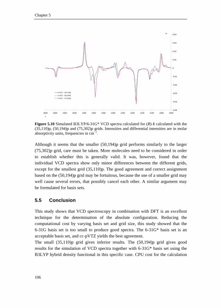
Chapter 5
106
Figure 5.10 Simulated B3LYP/6-31G* VCD spectra calculated for (R)-1 calculated with the (35,110)p, (50,194)p and (75,302)p grids. Intensities and differential intensities are in molar absorptivity units, frequencies in cm−1. Although it seems that the smaller (50,194)p grid performs similarly to the larger (75,302)p grid, care must be taken. More molecules need to be considered in order to establish whether this is generally valid. It was, however, found that the individual VCD spectra show only minor differences between the different grids, except for the smallest grid (35,110)p. The good agreement and correct assignment based on the (50,194)p grid may be fortuitous, because the use of a smaller grid may well cause several errors, that possibly cancel each other. A similar argument may be formulated for basis sets. 5.5 Conclusion
This study shows that VCD spectroscopy in combination with DFT is an excellent technique for the determination of the absolute configuration. Reducing the computational cost by varying basis set and grid size, this study showed that the 6-31G basis set is too small to produce good spectra. The 6-31G* basis set is an acceptable basis set, and cc-pVTZ yields the best agreement. The small (35,110)p grid gives inferior results. The (50,194)p grid gives good results for the simulation of VCD spectra together with 6-31G* basis set using the B3LYP hybrid density functional in this specific case. CPU cost for the calculation
-0.05
-0.04
-0.03
-0.02
-0.01
0
0.01
0.02
0.03
0.04
10001050110011501200125013001350140014501500155016001650
ν
6-31G* - (35,110)p
6-31G* - (50,194)p
6-31G* - (75,302)p
Δε

Hydroxymethyl dihydro-dioxinopyridine
References p.108 107
of the spectroscopic properties is approximately 30% less than those for the standard Gaussain98 (75,302)p grid. Although this study suggests that this grid would be an acceptable choice, care should be taken. Rotational invariance may be lost, which is not only unphysical but will also influence the calculated Boltzmann distribution. On the other hand, VCD spectra were found to be very similar for the (50,194)p and (75,302)p grids. More molecules should be tested to establish whether this is not due to a fortuitous cancellation of errors.‡ The use of the overlap integral as a quantitative measure for the similarity of VCD spectra is very useful, but one has to be careful in drawing conclusions on solely the value of the overlap integral, especially when anomalies are observed. The next step will be the tuning of this overlap index to make it proximity sensitive.
‡ No further efforts were taken to investigate the applicability of sparser grids, because further research showed that the rotational invariance could not be preserved.

Chapter 5
108
5.6 Reference list
1. Ariens, E. J. Med. Res. Rev. 1986, 6, 451-466.
2. Aamouche, A.; Devlin, F. J.; Stephens, P. J. J. Am. Chem. Soc. 2000, 122, 2346-2354.
3. Specht, K. M.; Nam, J.; Ho, D. M.; Berova, N.; Kondru, R. K.; Beratan, D. N.; Wipf, P.; Pascal, R. A.; Kahne, D. J. Am. Chem. Soc. 2001, 123, 8961-8966.
4. Parker, D. Chem. Rev. 1991, 91, 1441-1457.
5. Cheeseman, J. R.; Frisch, M. J.; Devlin, F. J.; Stephens, P. J. Chem. Phys. Lett. 1996, 252, 211-220.
6. Devlin, F. J.; Stephens, P. J.; Cheeseman, J. R.; Frisch, M. J. J. Phys. Chem. A 1997, 101, 9912-9924.
7. Stephens, P. J.; Devlin, F. J.; Chabalowski, C. F.; Frisch, M. J. J. Phys. Chem.-US 1994, 98, 11623-11627.
8. Stephens, P. J.; Ashvar, C. S.; Devlin, F. J.; Cheeseman, J. R.; Frisch, M. J. Mol. Phys. 1996, 89, 579-594.
9. Stephens, P. J.; Devlin, F. J. Chirality 2000, 12, 172-179.
10. Ashvar, C. S.; Stephens, P. J.; Eggimann, T.; Wieser, H. Tetrahedron-Asymmetr. 1998, 9, 1107-1110.
11. van Emelen, K.; de Bruyn, M. F. L.; Alcazar-Vaca, M. J.; Andres-Gil, J. I.; Fernandez-Gadea, F. J.; Matesanz-Ballesteros, M. E.; Bartolome-Nebreda, J. M. WO 2001098306, 2001.
12. Soukri, M.; Lazar, S.; Akssira, M.; Guillaumet, G. Org. Lett. 2000, 2, 1557-1560.
13. Polavarapu, P. L. Spectroscopy 1994, 9, 48-55.
14. Allinger, N. L.; Yuh, Y. H.; Lii, J. H. J. Am. Chem. Soc. 1989, 111, 8551-8566.
15. Allinger, N. L. MM3(96), 1996

Hydroxymethyl dihydro-dioxinopyridine
109
16. Bultinck, P.; Van Alsenoy, C.; Goeminne, A.; Van de Vondel, D. J. Phys. Chem. A 2000, 104, 11801-11809.
17. Frisch, M. J.; Trucks, G. W.; Schlegel, H. B.; Scuseria, G. E.; Robb, M. A.; Cheeseman, J. R.; Montgomery Jr, J. A.; Vreven, T.; Kudin, K. N.; Burant, J. C.; Millam, J. M.; Iyengar, S. S.; Tomasi, J.; Barone, V.; Mennucci, B.; Cossi, M.; Scalmani, G.; Rega, N.; Petersson, G. A.; Nakatsuji, H.; Hada, M.; Ehara, M.; Toyota, K.; Fukuda, R.; Hasegawa, J.; Ishida, M.; Nakajima, T.; Honda, Y.; Kitao, O.; Nakai, H.; Klene, M.; Li, X.; Knox, J. E.; Hratchian, H. P.; Cross, J. B.; Bakken, V.; Adamo, C.; Jaramillo, J.; Gomperts, R.; Stratmann, R. E.; Yazyev, O.; Austin, A. J.; Cammi, R.; Pomelli, C.; Ochterski, J. W.; Ayala, P. Y.; Morokuma, K.; Voth, G. A.; Salvador, P.; Dannenberg, J. J.; Zakrzewski, V. G.; Dapprich, S.; Daniels, A. D.; Strain, M. C.; Farkas, O.; Malick, D. K.; Rabuck, A. D.; Raghavachari, K.; Foresman, J. B.; Ortiz, J. V.; Cui, Q.; Baboul, A. G.; Clifford, S.; Cioslowski, J.; Stefanov, B. B.; Liu, G.; Liashenko, A.; Piskorz, P.; Komaromi, I.; Martin, R. L.; Fox, D. J.; Keith, T.; Al-Laham, M. A.; Peng, C. Y.; Nanayakkara, A.; Challacombe, M.; Gill, P. M. W.; Johnson, B.; Chen, W.; Wong, M. W.; Gonzalez, C.; Pople, J. A. Gaussian98, Revision A6; Gaussian, Inc.: Pittsburgh, 1998.
18. Becke, A. D. J. Chem. Phys. 1993, 98, 5648-5652.
19. Lee, C. T.; Yang, W. T.; Parr, R. G. Phys. Rev. B-Condens. Matter 1988, 37, 785-789.
20. Hehre, W. J.; Radom, L.; Schleyer, P. R.; Pople, J. A. Ab initio molecular orbital theory; Wiley: 1986.
21. Gill, P. M. W.; Johnson, B. G.; Pople, J. A. Chem. Phys. Lett. 1993, 209, 506-512.
22. Murray, C. W.; Handy, N. C.; Laming, G. J. Mol. Phys. 1993, 78, 997-1014.
23. Frisch, A. E.; Frisch, M. J.; Trucks, G. Gaussian 98 User's Reference; 5th ed.; Gaussian, Inc.: Pittsburgh, 1998.
24. Stephens, P. J. Vibrational circular dichroism spectroscopy: A new tool for the stereochemical characterization of chiral molecules. In Computational medicinal chemistry for drugs discovery, Bultinck, P., De Winter, H., Langenaeker, W., Tollenaere, J. P., Eds.; Marcel Dekker, Inc.: New York, 2004; pp 699-725.
25. McQuarrie, D. A. Statistical Thermodynamics; Harper and Row: New York, 1973.

Chapter 5
110
26. Schellman, J. A. Chem. Rev. 1975, 75, 323-331.
27. Johnson, B. G.; Gill, P. M. W.; Pople, J. A. Chem. Phys. Lett. 1994, 220, 377-384.
28. Johnson, B. G.; Frisch, M. J. Chem. Phys. Lett. 1993, 216, 133-140.
29. Scott, A. P.; Radom, L. J. Phys. Chem.-US 1996, 100, 16502-16513.
30. The neighborhood similarities are also computed and can be found in Supplementary Material

References p.136 111
6 determination of the AC of
three as-hydrindacene
compounds by VCD
Equation Chapter 6 Section 1
6.1 Introduction
Because the absolute configuration of molecules plays a dominant role in many fields of chemistry, methods to establish absolute configurations are of prime importance. One of the techniques that is continuously gaining more attention is the measurement of the vibrational circular dichroism (VCD). Essentially, VCD is based on the fact that when a molecule is irradiated with circularly polarized infrared radiation, different absolute configurations will exhibit different spectra. The most pictorial case is that of two enantiomers. Both enantiomers of a molecule will
Kuppens, T.; Vandyck, K.; Van der Eycken, J.; Herrebout, W.; van der Veken, B. J.; Bultinck, P. J. Org. Chem. 2005, 70, 9103-9114.

Chapter 6
112
exhibit the same unpolarized infrared (IR) spectrum. When using circularly polarized IR radiation and measuring the spectrum with left and right circularly polarized light separately, the differential absorbance spectrum will exhibit mirror symmetry. Therefore, although the location of the absorbance peaks remains the same in VCD as in unpolarized IR spectra, in VCD the peaks have different sign. As a result, a VCD spectrum contains information on the absolute configuration of a molecule. The interpretation of an experimental VCD spectrum and its connection with a specific stereochemistry has long remained a difficult task, however. A breakthrough was realized when Stephens et al. developed and implemented a quantum chemical algorithm for the computation of VCD spectra.1-3 This has contributed greatly to the increasing popularity of the VCD technique. Essentially, one performs the necessary VCD calculations using some quantum chemical code for the different possible stereoisomers, and subsequently compares the resulting theoretical spectrum with the experimental one. Despite this conceptually simple approach, some problems remain in the routine application of VCD, so it remains important to check the outcome of the VCD assignments, if possible, with other ways of determining absolute configurations.3-6 Some of the problems mentioned are related to the quantum chemical methodology used.2,5,7-11 Density functional theory (DFT) has previously been shown to give gratifying agreements between theory and experiment, but basis set effects can still play an important role.7,12,13 The advent of commercially available VCD spectrometers and the implementation of the VCD algorithms in widely available software packages, together with the increase in speed and power of computers will only extend the range of molecules that can be handled with the VCD technique. In this paper, a vibrational circular dichroism study on three 1,8-disubstituted as-hydrindacenes is presented i.e. (+)-1,2,3,6,7,8-hexahydro-as-indacene-1,8-diol ((+)-1), (+)-8-hydroxy-3,6,7,8-tetrahydro-2H-as-indacen-1-one ((+)-2) and (−)365-1,2,7,8-di-epoxy-3,6-dihydro-as-indacene ((−)-3).‡ The VCD assignments are checked against stereochemistry information based on ECD measurements and/or predictions based on the applied asymmetric methods in the synthetic route.14
‡ (+)-1: 20
Dα = +70.5 (c = 1.09, CHCl3, >99% ee); (+)-2: 25Dα = +98.2 (c = 1.04, CHCl3, >99 %
ee); (−)365-3: 25365α = −128.6 (c = 0.99, CHCl3, >99% ee)

AC of three as-hydrindacene compounds
References p.136 113
HOOH HOO
(1S,8S)-1 (8S)-2
OO
(1R,2S,7S,8R)-3
12
3
45
6
78
Figure 6.1 (+)-1,2,3,6,7,8-hexahydro-as-indacene-1,8-diol ((+)-1), (+)-8-hydroxy-3,6,7,8-tetrahydro-2H-as-indacen-1-one ((+)-2) and (−)365-1,2,7,8-di-epoxy-3,6-dihydro-as-indacene ((−)-3) Compounds 1–3 provide a chiral synthetic platform for the synthesis of a new class of rigid enantiopure hexahydro-as-indacene based chiral ligands for application in asymmetric catalysis.15 The as-hydrindacenes can be viewed as C2-symmetric analogues of indane systems which themselves have found numerous applications in asymmetric synthesis. Derivatives of compounds 1 were recently studied with the circular dichroism exciton chirality method.14 The determined absolute configurations of (+)-1 and (+)-2 are in agreement with what one would predict on the basis of the applied asymmetric reduction. 6.2 Results and discussion
6.2.1 Synthesis
Asymmetric transfer hydrogenation of the C2-symmetric prochiral diketone 4 applying an in situ prepared catalyst (A) derived from commercial (1S,2S)-(+)-N-p-tosyl-1,2-diphenylethylenediamine and [RuCl2(η6-cymene)]2 in a 5:2 formic acid-triethylamine mixture,16 resulted in alcohols (+)-1 and (+)-2 in good yield and high enantiomeric excess.14 Depending on the catalyst loading, reaction time and reaction temperature, (+)-1 or (+)-2 could be isolated as the main product (Scheme 6.1). The reduction is expected to yield the (S)-alcohols using the (S,S)-Ts-DPEN ligand by analogy with the reduction of indanone to (S)-indanol with the same ligand. Furthermore, reduction of 4 with NaBH4 in MeOH provided a 3/1 mixture of meso/(±)-1 alcohols in 99% yield. Concentration sensitive dehydration17 in the presence of no more than 1% p-TSA yielded one C2-symmetric isomer 5. This prochiral alkene can be transformed into the bisepoxide 3 using the low temperature

Chapter 6
114
Jacobsen epoxidation conditions.18 Noteworthy is the isomerisation of diene 5 by NMO at room temperature, emphasizing the importance of adding 5 at low temperature (−78 °C) to the mixture of catalyst and NMO, not at room temperature. The use of the (R,R)-catalyst allows to predict the absolute configuration to be (1R,2S) deduced from the formation of (1S,2R)-indene oxides when using the (S,S)-Jacobsen catalyst.19,20
OO
(+)-(1S,8S)-1 (+)-(8S)-2
4
NaBH4, MeOH, rt, 1h
1% p-TSA, benzene, 80°C, 160 min.
5
A
RuCl
H2NNTs
Ph
Ph
N N
OO
tBu
tBuMn
CltBu
tBu
meso/(±)-1 3/1 89%
99 %
Ref. 14 Ref. 14
Mn-(R,R)-Salen
Mn-(R,R)-salen, m-CPBA, NMO, –78°C, 110 min.
77 % yield > 98 % ee
(–)365-(1R,2S,7S,8R)-3
1 % A3 % A
Scheme 6.1 6.2.2 IR and VCD spectroscopy
The IR and VCD spectra for (+)-2 and (−)-3 were recorded in a demountable cell with KBr windows and a 105 µm spacer. The spectra for (+)-1 were recorded in a CaF2 cell with a 200 µm spacer. The unpolarized IR absorbance spectra were recorded at a resolution of 4 cm−1, the VCD spectra were recorded on a Bruker IFS 66v/S FTIR interferometer coupled to a Bruker PMA37 VCD module21 at a resolution of 6 cm−1. To improve the VCD S/N ratio an 1830 cm−1 long wave-pass filter was used.

AC of three as-hydrindacene compounds
References p.136 115
The collection time for the VCD spectrum was 2h each, in 4 blocks of 30 minutes. (+)-1 was dissolved in CDCl3 at a concentration of 0.11 M. For (+)-2, CDCl3 was used as solvent at a concentration of approximately 0.19 M. (−)-3 was dissolved in CDCl3 at a concentration of 0.20 M. To obtain a good estimate for the baseline artifacts, usually the VCD of the racemic mixture or both enantiomers is measured.22 As these are not always available, the VCD of the solvent, measured in the same conditions as the sample, is often a good approximation. In this study, a racemic mixture is only available for 1. For (±)-1, the VCD was measured at the exactly the same conditions as the solvent and the enantiopure solution. In Figure 6.2 the racemic and solvent corrected spectra are given. No significant differences involving the signs of any peaks can be seen.
1600 1500 1400 1300 1200 1100 1000-0.03
-0.02
-0.01
0.00
0.01
0.02
0.03 solvent corrected
ν
Δ ε
racemic mixture corrected
Figure 6.2 Baseline corrected VCD spectra for (+)-1, i.e., solvent corrected and racemic corrected. Differential intensities are in molar absorptivity units, frequencies in cm−1. 6.2.3 Computational methods
Because VCD spectra are composed of all contributions of the different conformations, a conformational search has to be performed. In the scope of absolute configuration (AC) determination by VCD, this is very important because of the strong dependence of VCD on the conformations present.23

Chapter 6
116
The conformational landscape is explored by molecular mechanics (MM) as well as DFT. A systematic search is carried out at B3LYP/6-31G* level. The aromatic ring of the as-hydrindacene skeleton is considered rigid, whereas the attached five-membered rings and exocyclic hydroxyl groups are considered flexible. The dihedral angles are varied in a 60° grid. A bump check and ring constraints24 assure that only the chemically sane starting structures are minimized on B3LYP/6-31G* level. Also, a systematic search (with a 10° dihedral grid) is performed with MMFF25 supplemented with a MM3 stochastic search26,27 to identify possible further minima. The located MMFF and MM3 geometries are then optimized at B3LYP/6-31G* level and supplemented with these found from the B3LYP/6-31G* systematic search. The DFT calculations are performed with Gaussian03 revision B528 in a distributed computing environment. The B3LYP4,29,30 functional is used together with the 6-31G* and cc-pVTZ basis sets. Eight additional functionals (B1LYP, B3LYP, B3P86, B3PW91, B98, BHandH, BHandHLYP, MPW1PW91, PBE1PBE)31 were employed using the 6-31G* basis set. The agreement between spectra is expressed via the similarity measures given in Equation (6.1) and (6.2). The normalized overlap in Equation (6.1) has been discussed earlier.7
2 2
( ) ( )
( ) ( )
f g dS
f d g d
σσυ υ υ
συ υ υ υ=
∫∫ ∫
(6.1)
( ) ( )
( ) ( ) ( ) ( )
fg fg
ff ff gg gg
w r c r drS
w r c r dr w r c r dr
σ =∫
∫ ∫ (6.2)
with
( ) 1
( ) 0
rw r if r l
lw r if r l
= − <
= ≥ (6.3)
and
( ) ( ) ( )ffc r f f r dυ υ υ= +∫ (6.4)
AC of three as-hydrindacene compounds
References p.136 117
The simple overlap is less robust because of the fundamental difference between experimental and simulated spectra. Although the theoretical frequencies are linearly scaled to correct for the harmonic approximation and basis set incompleteness, some peaks can still be shifted with respect to their corresponding experimental peak. A similarity measure that takes into account the neighborhood around the peaks, results in a more accurate and precise measure for their similarity. Equation (6.2)32 allows the consideration of the neighborhood with a width of −l and +l around each point in the spectrum. 6.2.4 Theoretical spectra
The dipole and rotational strengths are calculated for each DFT minimum on the potential energy surface. The results are single conformer line spectra, which are broadened using a Lorentzian band shape. Throughout the paper, Lorentzian broadening is always accomplished with a fwhm of 10 cm−1. Each minimum contributes to the total spectrum in a Boltzmann weighted manner. Conformational populations are based on the free energy. The enthalpy and free energy are calculated under the usual assumptions using standard thermochemical expressions.33 Appropriate frequency scaling factors are used to correct for the harmonic approximation. 6.2.5 Conformational analysis
Hexahydro-as-indacene-1,8-diol (1) Molecule 1 has two asymmetric carbon atoms. Because the sample of (+)-1, which is analyzed, is optically active (> 99% ee), the possible configurations of (+)-1 are limited to enantiomers 1(RR) or 1(SS) (mesomers 1(RS) and 1(SR), are identical and not optically active). The conformational space can be described by means of the orientation of the exocyclic substituents. The position of the alcohol group in the context of the five-membered ring is either designated as equatorial (“e”) or axial (“a”). For the CO(H) dihedral angle three typical minima in the torsion potential energy are observed, i.e., for dihedral angles of 60°, 180° and −60°. The dihedral angles are characterized as G, T, and G’ respectively for gauche clockwise, trans and gauche counter clockwise.

Chapter 6
118
Due to the C2-symmetry of 1, both substituents are indistinguishable, which is reflected in the conformational notation; the group-ring orientation and CO(H) bond torsion are given successively for both functional groups. In this fashion the global minimum of 1 can be written as eG’eG or eGeG’. The combined conformational searches, using different techniques that are described in §6.2.3, yielded 13 minima in total. These minima are shown in Figure 6.3.
1
2
3
4
5
6
7
8
9
10
11
12
13
Figure 6.3 Pictorial representation of the B3LYP/6-31G* PES minima for 1. Their corresponding notation and energy can be found in Table 6.1. For each minimum the B3LYP 6-31G* and cc-pVTZ relative total energies are given. Some higher energy cc-pVTZ conformers have a different energy order compared to the 6-31G*. Also, the expected eTaG minimum could not be located at the B3LYP/cc-pVTZ level. Starting from the B3LYP/6-31G* eTaG geometry, cc-pVTZ optimization converged in the eG’eG structure. Conformational populations are calculated based on the Boltzmann distribution using free energies at 298.15 K. From Table 6.1 it is clear that eG’eG and eG’eT are the dominant minima, the populations of both conformers summing more than 90%. This can be attributed to
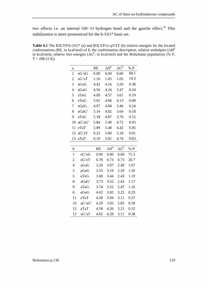
AC of three as-hydrindacene compounds
References p.136 119
two effects i.e. an internal OH···O hydrogen bond and the gauche effect.34 This stabilization is more pronounced for the 6-31G* basis set. Table 6.1 The B3LYP/6-31G* (a) and B3LYP/cc-pVTZ (b) relative energies for the located conformations (RE, in kcal/mol) of 1, the conformation description, relative enthalpies (ΔH0 in kcal/mol), relative free energies (ΔG0, in kcal/mol) and the Boltzmann populations (% P, T = 298.15 K).
a RE ΔΗ0 ΔG0 % P 1 eG’eG 0.00 0.00 0.00 84.12 eG’eT 1.10 1.05 1.05 14.3
13 aGeG 4.42 4.16 3.20 0.38 4 aGaG 4.50 4.24 3.47 0.24 5 aTeG 4.89 4.57 3.61 0.19 6 eTaG 5.01 4.66 4.13 0.08 7 eGeG 4.97 4.68 3.46 0.24 8 aGaG’ 5.14 4.82 3.64 0.18 9 aTaG 5.18 4.87 3.76 0.15 10 aG’aG’ 5.84 5.40 4.72 0.03 11 eTaT 5.89 5.48 4.42 0.05 12 aG’aT 6.22 5.80 5.18 0.01 13 aTaT 6.19 5.81 4.74 0.03
b RE ΔΗ0 ΔG0 % P 1 eG’eG 0.00 0.00 0.00 71.3 2 eG’eT 0.78 0.73 0.73 20.7 4 aGaG 3.20 3.07 2.49 1.07 3 aGeG 3.35 3.19 2.29 1.50 5 aTeG 3.68 3.44 2.43 1.19 8 aGaG’ 3.73 3.52 2.43 1.17 9 aTaG 3.74 3.52 2.47 1.10 6 eGeG 4.02 3.82 3.25 0.29 11 eTaT 4.28 3.94 3.11 0.37 10 aG’aG’ 4.29 3.93 2.85 0.59 12 aTaT 4.58 4.26 3.21 0.32 13 aG’aT 4.65 4.28 3.11 0.38

Chapter 6
120
Hydroxy-tetrahydro-H-as-indacen-one (2) In hydroxyketone 2, only one group-ring orientation and CO(H) bond torsion is present; a conformational notation comparable to the notation for compound 1 is used.
12 3
Figure 6.4 Pictorial representation of the B3LYP/6-31G* PES minima for 2. Conformation numbering conforms to that of Table 6.2. A combined stochastic MM3 and systematic MMFF search resulted in three B3LYP/6-31G* minima. These are shown in Figure 6.4 and listed in Table 6.2 accompanied with the 6-31G* and cc-pVTZ relative energies, enthalpies, free energies and Boltzmann populations. Remarkably, the expected minima eT, aT and aG’ are not found. Therefore a B3LYP/6-31G* systematic search around the C-C-O-H dihedral angle is performed for an equatorial and axial substitution. In Figure 6.5 the two dimensional PES is shown for the equatorial and axial scan, where the C-C-O-H dihedral angle is varied in steps of 1° and held fixed during optimization. As can be seen, no new minima are encountered. A transition from the axial surface to the equatorial surface can be observed in the proximity of the global minimum. This minimum is stabilized due to a strong internal OH···O hydrogen bond (1.95 Å – B3LYP/cc-pVTZ). Table 6.2 The B3LYP/6-31G* (a) and B3LYP/cc-pVTZ (b) relative energies for the localized conformations (RE, in kcal/mol) of 2, the conformation description, relative enthalpies (ΔH0, in kcal/mol), relative free energies (ΔG0, in kcal/mol), and the Boltzmann populations (% P, T = 298.15 K).
a RE ΔΗ0 ΔG0 % P 1 eG’ 0.00 0.00 0.00 100.0 2 aG 6.85 6.59 5.75 0.00 3 eG 8.19 7.87 6.75 0.00
b RE ΔΗ0 ΔG0 % P 1 eG’ 0.00 0.00 0.00 99.97 2 aG 5.97 5.73 4.90 0.03 3 eG 7.41 7.17 6.03 0.00

AC of three as-hydrindacene compounds
References p.136 121
0 30 60 90 120 150 180 210 240 270 300 330 360
0
1
2
3
4
5
6
7
8
9
10
11
E
C-C-O-H torsion
Axial scan Equatorial scan
eG'
aG
eG
'eqT'
'axT'
Figure 6.5 PES scan (C-C-O-H torsion) at B3LYP/6-31G* level of the equatorial and axial surface of 2 in steps of 1°. The dihedral angle is held fixed during optimization. Relative energies are in kcal/mol. Di-epoxy-dihydro-as-indacene (3) Because the four stereocentra of 3 are in a ring-attached epoxide system, they are two-by-two correlated. Due to the optical activity of the molecule, only the 3(RS,SR) and 3(SR,RS) enantiomers are likely. Due to the rigidity of compound 3 only one conformation could be found (depicted in Figure 6.6) using a stochastic and systematic search, as described in the §6.2.3.
Figure 6.6 Pictorial representation of the B3LYP/6-31G* PES minimum for 3.

Chapter 6
122
6.2.6 IR and VCD spectra
In Figures 6.7 and 6.8, the Lorentzian fitted experimental IR and VCD spectra of (+)-1 are given (residual fitting errors are given in Figure S6.1 – Supplementary Material). From the Boltzmann populations in Table 6.1 it can be seen that only two conformations have a considerable contribution. All conformations, however, are taken into account to simulate the spectra. Only eG’eG and eG’eT are needed to assign the experimental bands. Fundamentals designated as a, originate from conformation eG’eG, those designated as b represent eG’eT. No label is used when fundamentals of both conformations coincide or have a very small frequency separation. In Figures 6.7 and 6.8 the simulated spectra are shown for (1S,8S)-1. The B3LYP/6-31G* theoretical frequencies are uniformly scaled with a factor of 0.967; the B3LYP/cc-pVTZ spectra with a factor 0.977. The experimental assignments could be performed relatively easy due to the good agreement between theory and experiment, although peak broadening makes the assignment of the low intensity peaks (38–52) somewhat less straightforward. The peak assignment is primarily based on the IR spectrum. Nevertheless, due to the extra discriminating power provided by VCD, that is, the sign of intensity, some unresolved IR bands could be localized, because of their corresponding resolved VCD bands. The extensive assignment tables can be found in Supplementary Material, i.e., Tables S6.1 and S6.2.

AC of three as-hydrindacene compounds
References p.136 123
1500 1400 1300 1200 1100 10000
40
80
120
160
200
ν
ε
(i)
0
50
100
150
200
250
30037
ε
(ii) 54b5862
/61/
60
59 57
56a
56b
55a
55b54a
53
4749/4
8
46a
46b/
45/4
4a
44b 4342 41
/40b
40a/
39/3
8b
38a
36
35
34
5052/5
1
37
54b58
62/6
1/60
59 57
56a
56b
55a
55b 54a
53
4749
/48
46/4
5/44
a
44b/
43a
43b42 41
40a/
39/3
8b
38a
36
35
3451
a/50
52/5
1b
0
50
100
150
200
250
300
40b
ε
(iii)
59 5856/55a
57 55b
54/53
52b
51b/
52a
51a
5049
47
46/4
5/44
a
44b/
43
42 41
40a/
38/3
940
b
36 35
34
62/6
1/60
37
Figure 6.7 Lorentzian fitted unpolarized IR absorption spectrum for (+)-1 (i), B3LYP/6-31G* (ii) and B3LYP/cc-pVTZ (iii) simulated IR spectrum for (1S,8S)-1. Intensities are in molar absorptivity units, frequencies in cm−1.
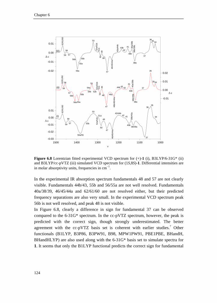
Chapter 6
124
1500 1400 1300 1200 1100 1000-0.03
-0.02
-0.01
0.00
0.01
ν
Δ ε
(i)
-0.01
0.00
0.01
0.02
Δ ε
(ii)
46/4
5/44
a
37
62/6
1/60
59
58
57
56a/55
55b
53
52a/
51b
51a
50
49
47
43/44b42 41
40b
39b/
40a
38/39a
3635
34
41
38b/
39b48
51a
535862/6
1/60
59
57
56a
56b
55a
55b
54a
54b 52b
47
49
46a
46b/
45/4
4a
44b 43 4240b
40a/
39b
38a
37
36
3534
5052
a/51
b
-0.02
-0.01
0.00
0.01
Δ ε
(iii)41
38b/
39b
48
51a
53
58
62/6
1/60
59 57
56a
56b
55a
55b
47
49
46/4
5/44
a
43a/
44b
43b42
40b
40a/
39b
38a
37
363534
50
52a/
51b
Figure 6.8 Lorentzian fitted experimental VCD spectrum for (+)-1 (i), B3LYP/6-31G* (ii) and B3LYP/cc-pVTZ (iii) simulated VCD spectrum for (1S,8S)-1. Differential intensities are in molar absorptivity units, frequencies in cm−1. In the experimental IR absorption spectrum fundamentals 48 and 57 are not clearly visible. Fundamentals 44b/43, 55b and 56/55a are not well resolved. Fundamentals 40a/38/39, 46/45/44a and 62/61/60 are not resolved either, but their predicted frequency separations are also very small. In the experimental VCD spectrum peak 56b is not well resolved, and peak 48 is not visible. In Figure 6.8, clearly a difference in sign for fundamental 37 can be observed compared to the 6-31G* spectrum. In the cc-pVTZ spectrum, however, the peak is predicted with the correct sign, though strongly underestimated. The better agreement with the cc-pVTZ basis set is coherent with earlier studies.7 Other functionals (B1LYP, B3P86, B3PW91, B98, MPW1PW91, PBE1PBE, BHandH, BHandHLYP) are also used along with the 6-31G* basis set to simulate spectra for 1. It seems that only the B1LYP functional predicts the correct sign for fundamental

AC of three as-hydrindacene compounds
References p.136 125
37. This functional also predicts fundamental 54, which is experimentally not resolved, to be positive in agreement with the cc-pVTZ basis set. When looking at the overall performance of the various functionals, only BHandH and BHandHLYP perform rather poorly. The other functionals have a comparable performance. The B3LYP functional has the best overall agreement (Figures S6.2 and S6.3 in Supplementary Material). In Table S6.7a (Supplementary Material) the neighborhood overlap (Equation (6.2)) between experimental and simulated IR/VCD spectra is given for different functionals. This type of overlap takes into account the local shift of the simulated band with respect to the experimental one. In addition, the scaling factor is given for which the normalized overlap between experimental and simulated IR spectra is maximized. The overlap is calculated for the 1700–1000 cm−1 wavenumber interval.
3700 3600 3500 3400 33000
20
40
60
80
100
ε
ν
32mM
OOHH
0.11M
81mM
48mM
Figure 6.9 Infrared spectrum in the OH stretch region for different concentrations of 1 (0.11 M, 81 mM, 48 mM, and 32 mM). The dashed line is the B3LYP/6-31G* simulated spectrum. Intensities are in molar absorptivity units, frequencies in cm−1. For 1, intermolecular interactions with solvent or solute molecules are possible via the OH groups, which could perturb the spectra notably.35 These interactions are not taken into account in our calculations, as these are performed on isolated molecules. In Figure 6.9 the IR spectra in the OH stretch region for 4 different concentrations are given i.e. 0.11 M (saturated solution), 81 mM, 48 mM, and 32 mM. Two OH

Chapter 6
126
stretch bands can be observed, i.e. an unresolved doublet due to non-interacting OH groups, and a doublet at 3589 cm−1 caused by the OH stretching involved in OH···O intramolecular hydrogen bonds. Doublets are due to the two most significant conformations. Figure 6.9 also contains the B3LYP/6-31G* simulated spectrum. The predicted frequencies for the OH stretching fundamental in the OH···O intramolecular hydrogen bond in conformation eG’eG and eG’eT nearly coincide, giving rise to only one peak. The broad band at 3513 cm−1 is due to self-association (hydrogen bonding between different solute molecules). The intensity of this band becomes somewhat smaller with lower concentrations. Comparing its intensities with those of the two monomeric bands, it is clear that self-association is less important. Furthermore, there is no concentration effect observed for the VCD spectra of the concentration series. Given the excellent agreement between the experimental and simulated spectra, the absolute configuration of (+)-1 can be assigned as (1S,8S)-1. This is in agreement with earlier ECD studies.14 In Figures 6.10 and 6.11 the Lorentzian fitted experimental IR and VCD spectra of (+)-2 are shown (residual fitting errors are given in Figure S6.1 – Supplementary Material) simultaneously with the B3LYP/6-31G* and B3LYP/cc-pVTZ simulated spectra for the S enantiomer of compound 2. The 6-31G* and cc-pVTZ frequency scaling factors used are 0.967 and 0.977 respectively. Based on the populations (Table 6.2) it can be seen that only conformation eG’ should be considered when assigning the peaks in the experimental spectrum. This assignment was based on the B3LYP/6-31G* and cc-pVTZ calculations. The extensive assignment tables can be found in Supplementary Material, i.e., Tables S6.3 and S6.4.

AC of three as-hydrindacene compounds
References p.136 127
1600 1400 1200 10000
50
100
150
200
250
300
350
ν
ε
(i)
60
5958 57
56
55/5
4
53
52
5150
49
48
47/4
6
45/4
4
43
4140 39 38
/37/
36
3534
33
0
50
100
150
200
250
300
350
44
ε
(ii)
60
5958 57
/56/
55
54
53
52 51
50
49
48
47/4
6
45 43
42/4
1
40 39
38/3
7/36
35
3433
0
50
100
150
200
250
300
350
ε
(iii)
44
60
5958 57
/56
55/5
4
5352
51
50
49
48
47/4
6
4543
42/4
1
40 39
38/3
7/36
35
34
33
Figure 6.10 Lorentzian fitted unpolarized IR absorption spectrum for (+)-2 (i), B3LYP/6-31G* (ii) and B3LYP/cc-pVTZ (iii) simulated IR spectrum for (S)-2. Intensities are in molar absorptivity units, frequencies in cm−1.

Chapter 6
128
1700 1600 1500 1400 1300 1200 1100 1000
-0.02
-0.01
0.00
0.01
0.02
0.03
53
ν
Δ ε(i)
59
57
56
5554
52
51
50
49
48
47/4645
44
43
4140
39
37/3
8
36 35
34
33
-0.02
-0.01
0.00
0.01
0.02
0.03
58
Δ ε(ii)
60
x40
-0.02
-0.01
0.00
0.01
0.02
0.03
55
35
53
Δ ε(iii)
5957
/56/
55
54
52
51
50
49
48
47/4
6
45
44
43
42/4
1
40
39
37/3
8
36
35
34
33
60
5853
59
57/5
6
54
52
51
50
49
48
47/4
6
45
44
43
42/4
1
40
39
37/3
8
36
34
33
60 x60
Figure 6.11 Lorentzian experimental VCD spectrum for (+)-2 (i), B3LYP/6-31G* (ii) and B3LYP/cc-pVTZ (iii) simulated VCD spectrum for (S)-2. Differential intensities are in molar absorptivity units, frequencies in cm−1. In the experimental IR spectrum it can be seen that peaks 36/37/38, 45/44 and 54/55 are not resolved, which is in agreement with the predicted small frequency separation. Peaks 53, 51, 50 and 42 are not visible. In the experimental VCD spectrum peaks 46/47, and 38/37 are not resolved, in agreement with simulations. Peaks 58, 53 and 42 are not visible. When looking at the signs of the VCD peaks for (+)-2 in Figure 6.11, it can be seen that the sign of fundamental 35 is not correctly predicted for both basis sets. For 6-31G* fundamentals 56 and 57 have the wrong predicted sign. For the cc-pVTZ simulated spectra, fundamental 59 is erroneously predicted, i.e. slightly positive. However, predicted VCD intensities for fundamental 59 are very small, and the noise level in that area of the experimental spectrum is rather high. Different functionals are used to simulate spectra at 6-31G* level. None of the functionals manage to correctly predict the sign for fundamental 35. B3P86,

AC of three as-hydrindacene compounds
References p.136 129
MPW1PW91 and PBE1PBE succeed in calculating the correct signs for fundamentals 57 and 56 but fail for fundamental 55. An overview of the overall performance of the different functionals, in given in Supplementary Material, i.e. Table S6.7 (neighborhood overlap along with the scaling factor) and Figures S6.5 and S6.6 (simulated IR and VCD spectra). It shows again that, for our purposes, BHandH and BHandHLYP have a bad performance at 6-31G* level. The other functionals perform similarly.
3700 3600 3500 3400 3300 32000
10
20
30
40
50
60
OOH H CCl3ε
ν
eG' ... CHCl3
eG' 100%
aG 50%eG 50%
Figure 6.12 Infrared spectrum in the OH stretch region for different concentrations of 2 (0.19 M, 0.14 M, 95 mM, and 57 mM). The dashed lines are B3LYP/6-31G* simulated spectra. Intensities are in molar absorptivity units, frequencies in cm−1. In the OH stretch region three distinct bands can be observed. One band at 3672 cm−1, a small shoulder at 3594 cm−1 and a broad asymmetric band at 3430 cm−1. In agreement with the B3LYP/6-31G* “force field” calculations, the OH stretch band for the intramolecular hydrogen bonded system is shifted to a lower wavenumber and can be found at approximately 3430 cm−1 (Figure 6.12). This band is asymmetric and relatively broad. As can be seen, there is no concentration effect, meaning that this broadening can not be attributed to self-association, as diluting affects the aggregation. However, CDCl3 solvent molecules can interact with the solute (CCl3D···O(H)−C), further reducing the OH stretch frequency. This was confirmed at B3LYP/6-31G* level, taking this interaction explicitly into account (Figure 6.12). In this manner the asymmetric broad band can be explained. The band

Chapter 6
130
at 3672 cm−1 and its small shoulder can be explained by taking into account the conformations without intramolecular hydrogen bonding. Based on gas-phase calculations their contributions are insignificant compared to the global minimum (Table 6.2), but due to solvent stabilization these conformations apparently gain importance. More evidence can be found at the C=O stretch region, where a doublet is observed in the VCD spectrum (Figure 6.11, fundamental 60). However, the relative intensities of these stabilized conformation bands are low compared to those of the intramolecular hydrogen bonds. Calculations in which the experimental spectrum was reproduced by averaging the calculated VCD spectra and manual adjustment of the conformational populations, shows that the experimental spectra are largely dominated by the global minimum eG’. For the C−O(H) stretching mode, fundamental 35, the calculations always yield a positive VCD signal, while the experimental data clearly shows that for this mode a negative signal is present. A similar pattern is also observed for fundamental 37 in 1. The B3LYP/6-31G* calculations for 1 gives a wrong sign for fundamental 37. The calculations using the cc-pVTZ basis set yields a correct sign, but seriously underestimated the rotational strength. The agreement for some areas is not as excellent as for 1, but the overall agreement allows to conclude with high certainty that the absolute configuration of (+)-2 corresponds to (8S)-2. This is in agreement with the earlier ECD exciton chirality assignment and the prediction based on the selectivity of the asymmetric reduction of indanone with the same catalyst.14 In Figures 6.13 and 6.14, the Lorentzian fitted experimental IR and VCD spectra of (−)-3 are given (residual fitting errors are given in Figure S6.1 – Supplementary Material). Also the simulated spectra are shown for (1R,2S,7S,8R)-3. The B3LYP/6-31G* theoretical frequencies are uniformly scaled with a factor of 0.967; the B3LYP/cc-pVTZ spectra with a factor 0.977.
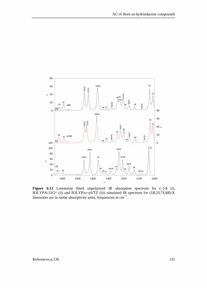
AC of three as-hydrindacene compounds
References p.136 131
1600 1500 1400 1300 1200 1100 10000
20
40
60
80
100
120
ν
ε
(i)
0
20
40
60
80
ε
(ii)
x1005655
54/5
352
/51
49/50
4847 46
/45
44
43/4
241
/40
39
38/3
7
36
35/3
4
33
32
0
20
40
60
80
42
ε
(iii)
56 55
54/53
52/51
50
4948 47
46/4544
43/42
41/40
39
38/37
36
35/34
33
x60
49/50
48 47 46/4
5
4443 41/4
0
39 38/3
7
36
35/3
4
33
32
54/5
3
52/5
1
5655
Figure 6.13 Lorentzian fitted unpolarized IR absorption spectrum for (−)-3 (i), B3LYP/6-31G* (ii) and B3LYP/cc-pVTZ (iii) simulated IR spectrum for (1R,2S,7S,8R)-3. Intensities are in molar absorptivity units, frequencies in cm−1.
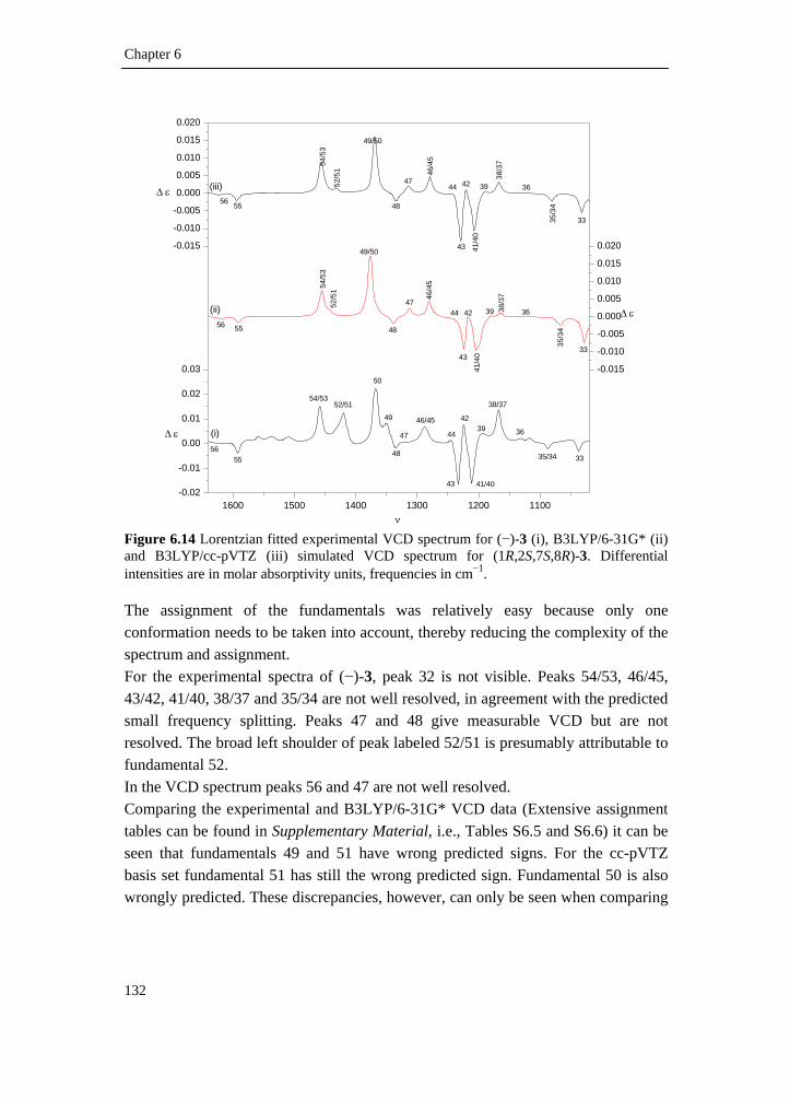
Chapter 6
132
1600 1500 1400 1300 1200 1100-0.02
-0.01
0.00
0.01
0.02
0.03
ν
Δ ε (i)
-0.015
-0.010
-0.005
0.000
0.005
0.010
0.015
0.020
Δ ε(ii) 42
49/50
48
47
46/4
5
44
43
41/4
0
39 38/3
7
36
35/3
4
33
54/5
352
/51
56 55
-0.015
-0.010
-0.005
0.000
0.005
0.010
0.015
0.020
Δ ε (iii)
33
43
5655
54/5352/51
50
49
48
47
46/45
44
42
41/40
39
38/37
36
35/34
42
49/50
48
47
46/4
5
44
43 41/4
0
39
38/3
7
36
35/3
4
33
54/5
3
52/5
1
56 55
Figure 6.14 Lorentzian fitted experimental VCD spectrum for (−)-3 (i), B3LYP/6-31G* (ii) and B3LYP/cc-pVTZ (iii) simulated VCD spectrum for (1R,2S,7S,8R)-3. Differential intensities are in molar absorptivity units, frequencies in cm−1. The assignment of the fundamentals was relatively easy because only one conformation needs to be taken into account, thereby reducing the complexity of the spectrum and assignment. For the experimental spectra of (−)-3, peak 32 is not visible. Peaks 54/53, 46/45, 43/42, 41/40, 38/37 and 35/34 are not well resolved, in agreement with the predicted small frequency splitting. Peaks 47 and 48 give measurable VCD but are not resolved. The broad left shoulder of peak labeled 52/51 is presumably attributable to fundamental 52. In the VCD spectrum peaks 56 and 47 are not well resolved. Comparing the experimental and B3LYP/6-31G* VCD data (Extensive assignment tables can be found in Supplementary Material, i.e., Tables S6.5 and S6.6) it can be seen that fundamentals 49 and 51 have wrong predicted signs. For the cc-pVTZ basis set fundamental 51 has still the wrong predicted sign. Fundamental 50 is also wrongly predicted. These discrepancies, however, can only be seen when comparing

AC of three as-hydrindacene compounds
References p.136 133
the rotational strengths and not in the broadened spectra because of the small frequency separations between mode 49/50 and 51/52 (Tables S6.5 and S6.6, Supplementary Material). Comparing the calculated rotational strengths for different functionals, it shows that fundamental 49 is predicted to have a wrong (negative) sign. The functionals which predict the sign of fundamental 51 correctly (B3P86, B3PW91, MPW1PW91 and PBE1PBE) fail to predict the sign correctly for fundamentals 44 and 52. All functionals have a comparable performance, apart from BHandH and BHandHLYP which have a bad performance. In Table S6.7 and Figures S6.6 and S6.7 (Supplementary Material) this is shown through the neighborhood overlap values for experimental and the simulated spectra. Comparing experimental spectra with simulated spectra, we can see an excellent agreement, allowing an assignment of the absolute configuration of (−)-3 to (1R,2S,7S,8R)-3. Comparing the performance of the basis sets for the three molecules, it shows again7,13 that the 6-31G* basis set is adequate to perform absolute configuration assignments, with the cc-pVTZ basis set being superior. This is shown in the above discussion, but is also clear from Table 6.3, where the neighborhood overlap (Equation (6.2)) is given for experimental IR/VCD spectra and the simulated spectra. The cc-pVTZ neighbourhood overlap values are all closer to 1 compared to the 6-31G* values indicating a better agreement with experiment. Table 6.3 Neighbourhood similarity (Sσ, in percent) for IR and VCD spectra for theory versus experiment for (a) 6-31G* and (b) cc-pVTZ basis set and maximizing scaling factor for default IR overlap.
a Sσ IR Sσ VCD σ 1 93.6 74.6 0.960 2 92.0 74.3 0.952 3 87.1 62.2 0.975
b Sσ IR Sσ VCD σ 1 97.2 79.5 0.977 2 93.8 80.4 0.965 3 94.1 80.6 0.978

Chapter 6
134
6.3 Conclusion
Absolute configurations of (+)-1, (+)-2 and (−)-3 were determined respectively as (1S,8S)-1, (8S)-2 and (1R,2S,7S,8R)-3. This was accomplished on B3LYP/6-31G* and cc-pVTZ level. cc-pVTZ spectra were proven to be superior to the 6-31G* spectra, which confirms earlier studies. Also, it is shown that small differences between theory and experiment are not the effect of the choice of functional, as the performance of most functionals is very comparable. The use of VCD to assign absolute configurations is a powerful method, which allows determination of the absolute configurations based on quantum chemical calculations and experimental spectra of dilute solutions. In contrast to the ECD determination for compound 1 and 2, the VCD method does not require extra synthesis steps to introduce chromophore groups in order to induce exciton coupling. 6.4 Supplementary material index
For this chapter Supplementary Material is provided. It can be downloaded from http://www.quantum.UGent.be/tksup.pdf Table S6.1 Assignment of the experimental peaks of (+)-1 (B3LYP/6-31G*) Table S6.2 Assignment of the experimental peaks of (+)-1 (B3LYP/cc-pVTZ) Table S6.3 Assignment of the experimental peaks of (+)-2 (B3LYP/6-31G*) Table S6.4 Assignment of the experimental peaks of (+)-2 (B3LYP/cc-pVTZ) Table S6.5 Assignment of the experimental peaks of (−)-3 (B3LYP/6-31G*) Table S6.6 Assignment of the experimental peaks of (−)-3 (B3LYP/cc-pVTZ) Table S6.7 Neighborhood similarity Sσ for theoretical versus experimental IR and VCD spectra using different functionals Figure S6.1 IR absorption and VCD spectrum for (+)-1, (+)-2 and (−)-3, including Lorentzian fit and residual fitting error Figure S6.2 Simulated (1S,8S)-1 IR DFT/6-31G* for different functionals and experimental spectra Figure S6.3 (1S,8S)-1 VCD DFT/6-31G* for different functionals and experimental spectra.

AC of three as-hydrindacene compounds
References p.136 135
Figure S6.4 Simulated (S)-2 IR DFT/6-31G* for different functionals and experimental spectra. Figure S6.5 Simulated (S)-2 VCD DFT/6-31G* for different functionals and experimental spectra. Figure S6.6 Simulated (1R,2S,7S,8R)-3 IR DFT/6-31G* for different functionals and experimental spectra. Figure S6.7 Simulated (1R,2S,7S,8R)-3 IR DFT/6-31G* for different functionals and experimental spectra. Figure S6.8 Mid IR and OH stretch region for (+)-2 in three different solvents. General experimental methods

Chapter 6
136
6.5 Reference list
1. Cheeseman, J. R.; Frisch, M. J.; Devlin, F. J.; Stephens, P. J. Chem. Phys.
Lett. 1996, 252, 211-220.
2. Devlin, F. J.; Stephens, P. J.; Cheeseman, J. R.; Frisch, M. J. J. Phys. Chem. A 1997, 101, 9912-9924.
3. Stephens, P. J.; Ashvar, C. S.; Devlin, F. J.; Cheeseman, J. R.; Frisch, M. J. Mol. Phys. 1996, 89, 579-594.
4. Stephens, P. J.; Devlin, F. J.; Chabalowski, C. F.; Frisch, M. J. J. Phys. Chem.-US 1994, 98, 11623-11627.
5. Stephens, P. J. Vibrational circular dichroism spectroscopy: A new tool for the stereochemical characterization of chiral molecules. In Computational medicinal chemistry for drugs discovery, Bultinck, P., De Winter, H., Langenaeker, W., Tollenaere, J. P., Eds.; Marcel Dekker, Inc.: New York, 2004; pp 699-725.
6. Wang, F.; Wang, Y.; Polavarapu, P. L.; Li, T. Y.; Drabowicz, J.; Pietrusiewicz, K. M.; Zygo, K. J. Org. Chem. 2002, 67, 6539-6541.
7. Kuppens, T.; Langenaeker, W.; Tollenaere, J. P.; Bultinck, P. J. Phys. Chem. A 2003, 107, 542-553.
8. Aamouche, A.; Devlin, F. J.; Stephens, P. J.; Drabowicz, J.; Bujnicki, B.; Mikolajczyk, M. Chem.-Eur. J. 2000, 6, 4479-4486.
9. Aamouche, A.; Devlin, F. J.; Stephens, P. J. J. Am. Chem. Soc. 2000, 122, 2346-2354.
10. Polavarapu, P. L.; Zhao, C. X.; Ramig, K. Tetrahedron-Asymmetr. 1999, 10, 1099-1106.
11. Wang, F.; Polavarapu, P. L.; Lebon, F.; Longhi, G.; Abbate, S.; Catellani, M. J. Phys. Chem. A 2002, 106, 5918-5923.
12. Freedman, T. B.; Cao, X. L.; Dukor, R. K.; Nafie, L. A. Chirality 2003, 15, 743-758.
13. Stephens, P. J.; Devlin, F. J. Chirality 2000, 12, 172-179.

AC of three as-hydrindacene compounds
137
14. Vandyck, K.; Matthys, B.; Van der Eycken, J. Tetrahedron Lett. 2005, 46, 75-78.
15. Catalytic Asymmetric Synthesis; 2nd ed.; Wiley-VCH: New York, 2000.
16. Fujii, A.; Hashiguchi, S.; Uematsu, N.; Ikariya, T.; Noyori, R. J. Am. Chem. Soc. 1996, 118, 2521-2522.
17. Moglioni, A. G.; Tombari, D. G.; Iglesias, G. Y. M. J. Chem. Research (S) 1998, 9, 606-607.
18. Palucki, M.; Pospisil, P. J.; Zhang, W.; Jacobsen, E. N. J. Am. Chem. Soc. 1994, 116, 9333-9334.
19. Kobayashi, T.; Tanaka, K.; Miwa, J.; Katsumura, S. Tetrahedron-Asymmetr. 2004, 15, 185-188.
20. Larrow, J. F.; Roberts, E.; Verhoeven, T. R.; Ryan, K. M.; Senanayake, C. H.; Reider, P. J.; Jacobsen, E. N. Org. Synth. 1999, 76, 46-56.
21. Urbanova, M.; Setnicka, V.; Volka, K. Chirality 2000, 12, 199-203.
22. Nafie, L. A. Appl. Spectrosc. 2000, 54, 1634-1645.
23. Polavarapu, P. L. Spectroscopy 1994, 9, 48-55.
24. Sadowski, J.; Schwab, C. H.; Gasteiger, J. 3D structure generation and conformational searching. In Computational medicinal chemistry for drugs discovery, Bultinck, P., De Winter, H., Langenaeker, W., Tollenaere, J. P., Eds.; Marcel Dekker, Inc.: New York, 2004; pp 151-212.
25. Halgren, T. A. J. Comput. Chem. 1996, 17, 490-519.
26. Allinger, N. L. MM3(96), 1996
27. Allinger, N. L.; Yuh, Y. H.; Lii, J. H. J. Am. Chem. Soc. 1989, 111, 8551-8566.
28. Frisch, M. J.; Trucks, G. W.; Schlegel, H. B.; Scuseria, G. E.; Robb, M. A.; Cheeseman, J. R.; Montgomery Jr, J. A.; Vreven, T.; Kudin, K. N.; Burant, J. C.; Millam, J. M.; Iyengar, S. S.; Tomasi, J.; Barone, V.; Mennucci, B.; Cossi, M.; Scalmani, G.; Rega, N.; Petersson, G. A.; Nakatsuji, H.; Hada, M.; Ehara, M.; Toyota, K.; Fukuda, R.; Hasegawa, J.; Ishida, M.; Nakajima, T.; Honda, Y.; Kitao, O.; Nakai, H.; Klene, M.; Li, X.; Knox, J. E.; Hratchian, H. P.; Cross, J. B.; Bakken, V.; Adamo, C.; Jaramillo, J.; Gomperts, R.; Stratmann,

Chapter 6
138
R. E.; Yazyev, O.; Austin, A. J.; Cammi, R.; Pomelli, C.; Ochterski, J. W.; Ayala, P. Y.; Morokuma, K.; Voth, G. A.; Salvador, P.; Dannenberg, J. J.; Zakrzewski, V. G.; Dapprich, S.; Daniels, A. D.; Strain, M. C.; Farkas, O.; Malick, D. K.; Rabuck, A. D.; Raghavachari, K.; Foresman, J. B.; Ortiz, J. V.; Cui, Q.; Baboul, A. G.; Clifford, S.; Cioslowski, J.; Stefanov, B. B.; Liu, G.; Liashenko, A.; Piskorz, P.; Komaromi, I.; Martin, R. L.; Fox, D. J.; Keith, T.; Al-Laham, M. A.; Peng, C. Y.; Nanayakkara, A.; Challacombe, M.; Gill, P. M. W.; Johnson, B.; Chen, W.; Wong, M. W.; Gonzalez, C.; Pople, J. A. Gaussian03, Revision B5; Gaussian, Inc.: Wallingford CT, 2004.
29. Becke, A. D. J. Chem. Phys. 1993, 98, 5648-5652.
30. Lee, C. T.; Yang, W. T.; Parr, R. G. Phys. Rev. B-Condens. Matter 1988, 37, 785-789.
31. Frisch, A. E.; Frisch, M. J.; Trucks, G. Gaussian 03 User's Reference; 5th ed.; Gaussian, Inc.: Pittsburgh, 2003.
32. De Gelder, R.; Wehrens, R.; Hageman, J. A. J. Comput. Chem. 2001, 22, 273-289.
33. McQuarrie, D. A. Statistical Thermodynamics; Harper and Row: New York, 1973.
34. Wolfe, S. Acc. Chem. Res. 1972, 5, 102-111.
35. He, J. T.; Polavarapu, P. L. Spectrochim. Acta A 2005, 61, 1327-1334.

References p.161 139
7 elucidation of the AC of
JNJ-27553292, a CCR2
receptor antagonist Equation Chapter 7 Section 1 7.1 Introduction
The chemokine receptor CCR2 has a central role in the establishment and maintenance of chronic inflammatory processes. CCR2 and its primary ligand, MCP1, represent a critical signaling pathway for the recruitment of peripheral blood monocytes to sites of immune-mediated inflammation, where they become inflammatory macrophages.1 Macrophages are among the predominant cell types found at sites of chronic inflammation, and clinical observations show a close correlation between lower macrophage burden and reduced severity of disease. The inhibition of the CCR2 receptor is a promising target for various inflammatory diseases such as rheumatoid arthritis, multiple sclerosis, chronic obstructive
Kuppens, T.; Herrebout, W.; van der Veken, B. J.; Corens, D.; De Groot, A.; Doyon, A.; Van Lommen, G.; Bultinck, P. Chirality 2006, 18, 609-620.

Chapter 7
140
pulmonary disease and atherosclerosis.1 Recently, a new class of CCR2 antagonists were described, i.e., the 2-mercapto-imidazoles2-5, with compound 1 being one of the most active representatives of this series. It was found that the CCR2 antagonistic activity resides primarily in one enantiomer hence the need to elucidate the absolute configuration for this compound. The synthesis of 1 is described in Scheme 7.1. Cl
ClNH2
Cl
ClHN
O
O
Cl
ClN
O
OO
Cl
ClN
O
OHS
N
Cl
ClN
O
OO
.HCl
a b
c
d
H
NaOO
OO
O
1 Scheme 7.1 Synthetic route to 2-mercaptoimidazole 1. Reagents and conditions (yields): a. Methylbromoacetate, Di-isopropyl-ethylamine (DIPEA), THF [room temperature, 1 days] (80%) b. HCOOH, xylene [reflux, 6 h] (100%) c. methyloxalate, NaOtBu, THF [room temperature, 20 h] d. KSCN, HCl–H2O, MeOH [60 °C, 20 h] (70% over c and d) Both enantiomers of 1 were prepared following Scheme 7.1, starting from the corresponding enantiomers of 1-(3’,4’-dichlorophenyl)-propanamine (5) that can be synthesized enantioselectively according to Scheme 7.2.6-8 Although 1-(3’,4’-dichlorophenyl)-propanol (3) has not been described before, very close analogues (phenyl and 4’-chlorophenyl) have been published.7,8 The more active enantiomer of 1 was found to be (−)-1, derived from amine (−)-5 that by analogy with the published data should have the S configuration. To confirm this assignment a vibrational circular dichroism (VCD) analysis was performed on amine (−)-5. The analysis of the antagonist 1 itself would not render the same reliability, due to the higher density of vibrational transition (and consequently more unresolved bands). The starting alcohol (+)-3 was analyzed to confirm the inversion of absolute configuration (step b in Scheme 7.2) unambiguously. VCD has become a good technique as an alternative for other

AC CCR2 receptor antagonist
References p.161 141
absolute configuration determination methods such as X-ray diffraction and NMR, and has proven its reliability for a wide range of molecules.9,10
Cl
Cl
O
HCl
Cl
OH
Cl
Cl
N3Cl
NH2
Cl
NHSO2CF3
NHSO2CF3
a
b
c
2 (+)-(R)-3
(–)-(S)-4(–)-(S)-5
catalyst
Scheme 7.2 Stereospecific synthesis of 1-(3,4-chloro-phenyl)-1-amino-propane. Reagents (yields) : a. Et2Zn, Ti(i-PropO)4, catalyst N,N'-((1S,2S)-cyclohexane-1,2-diyl)bis(trifluoromethanesulfonamide), toluene, −78 °C (100%) b. Diphenylphosphorylazide, 1,8-diazabicyclo[5.4.0]undec-7-ene, toluene (75%) c. Pt/C (10%), H2, methanol (75%). The circular dichroism (CD) phenomenon is in principle the differential absorption (by a molecular species) of left and right circularly polarized light.11 CD is only observable for chiral molecules or species for which the mirror image of a molecule cannot be brought in coincidence with itself. Vibrational CD applies circularly polarized infrared (IR) radiation. The first measurements of VCD date back to the early 1970s.12,13 Since then, the technique has improved continuously, and nowadays, VCD spectra for the 800–1800 cm−1 mid-IR region can be measured almost routinely.14 As VCD is a differential form of spectroscopy, intensities can be negative. The intensities of the VCD of enantiomers are equal in magnitude but opposite in sign. However, extracting the absolute configuration from the VCD spectra is not straightforward, but nevertheless can be done using quantum chemical calculations. A relatively fast and accurate algorithm was developed that allows to calculate VCD intensities15-17 using density functional theory (DFT).18 As a result, VCD spectra for

Chapter 7
142
molecules with known stereochemistry can be computed and compared to experimental spectra. The availability of VCD spectrometers and software that allows the calculation of VCD intensities makes VCD a highly practical method in the elucidation of the absolute configuration. Moreover, measurements can be done in diluted solutions, and no extra synthesis steps or additives are required, in contrast to other techniques.19 7.2 Methods
7.2.1 Preparation of the catalyst
To an ice-cold solution of trans-(1S,2S)-cyclohexyl diamine (5 g, 44 mmol) and di-isopropylethylamine in 250 ml of dichloromethane was added dropwise trifluoromethane sulfonylchloride (16.8 g, 100 mmol) in 50 ml of dichloromethane. The reaction mixture was allowed to warm to room temperature and stirred overnight. The reaction mixture was poured in water and the organic phase was washed three times with 100 ml of 1 N HCl. After drying and concentration of the organic phase 15.9 g of a very light yellow solid (96%) was obtained. Melting point 184–186 °C. 7.2.2 Preparation of (+)-(R)-1-(3’,4’-dichlorophenyl)-propanol (3)
A 3 liter flask was charged with 1 liter of dry toluene, the catalyst (2 g, 0.0053 mol) and Ti(i-PrO)4 (193 g, 0.68 mol). The resulting solution was degassed by three freeze-thaw cycles under argon. This solution was then heated to 40 °C for 20 minutes and cooled to −78 °C. Pure Et2Zn (85 g, 0.68 mol) was carefully transferred under argon via a large-gauge cannula into an addition funnel and then added over 20 minutes to the reaction mixture. The light orange solution was left 15 minutes and the aldehyde 2 (100 g, 0.57 mol), dissolved in toluene, was added dropwise over 30 minutes. The reaction mixture was allowed to slowly warm up to 0 °C over a few hours. After 4 h the reaction mixture was carefully quenched by addition of 1 M HCl. The aqueous layer was extracted with CH2Cl2 and the combined organic phases were filtered through celite, washed with water, dried over MgSO4 and concentrated to give 120 g of a light yellow liquid containing traces of toluene but otherwise pure
AC CCR2 receptor antagonist
References p.161 143
by GC-MS and NMR; 20Dα = +27 (c=0.47, CHCl3); IR 3346, 2966, 2933, 2877, 1687,
1587, 1466, 1383, 1029, 819 cm−1; 1H NMR (CDCl3, 360 MHz) δ (ppm) 7.42 (d, J=2.2 Hz, 1 H), 7.39 (d, J=8.4 Hz, 1 H), 7.14 (dd, J=2.2, 8.4 Hz, 1 H), 4.55 (t, J=6.6 Hz, 1 H), 2.30–2.10 (brd s, 1 H), 1.85–1.60 (m, 2 H), 0.89 (t, J=7.3 Hz, 3 H); 13C NMR (CDCl3, 90 MHz) δ (ppm) 144.7, 130.2, 127.9, 125.3, 74.6, 31.8, 9.8. 7.2.3 Preparation of (−)-(S)-4-(1-azidopropyl)-1,2-dichlorobenzene (4)
The alcohol 3 (26 g, 0.127 mol) and DPPA (42 g, 0.153 mol) were placed in a 1 liter flask containing 0.5 liter of dry toluene and the mixture was cooled to 0 °C. 1,8-diazabicyclo[5.4.0]undec-7-ene (DPU) (23.3 g, 0.153 mol) was added dropwise over 30 minutes. The reaction mixture was allowed to slowly warm-up to room temperature and further stirred for 12 h. The reaction mixture was diluted with toluene and washed three times with 200 ml each of 1M HCl. The organic phase was washed with water, dried over MgSO4, concentrated and purified by column chromatography on silica gel (elution with CH2Cl2 then with 1% MeOH in CH2Cl2) giving 23.5 g of a colorless liquid.
20Dα = −125 (c=0.58, CHCl3), IR (film) 2093 (s); 1H NMR (CDCl3, 360 MHz)
δ (ppm) 7.45 (d, J=8.4 Hz, 1 H), 7.39 (d, J=2.2 Hz, 1 H), 7.14 (dd, J=2.2, 8.4 Hz, 1 H), 4.33 (app. t, J=6.95 Hz, 1 H), 1.92–1.66 (m, 2 H), 0.93 (t, J=7.3 Hz, 3 H); 13C NMR (CDCl3, 90 MHz) δ (ppm) 140.1, 132.9, 132.2, 130.7, 128.9, 126.2, 66.6, 29.4, 10.5. 7.2.4 Preparation of (−)-(S)-1-(3’,4’-dichlorophenyl)-propanamine (5)
A solution of the azide 4 (50 g, 0217 mol) in methanol (800 ml) and Pt/C 5% (2 g) was placed in a Parr apparatus and flushed with three cycles of vacuum/hydrogen. The flask was then placed under 50 psi of hydrogen. The reaction was monitored by TLC. The catalyst was filtered-off and the solvent evaporated under reduced pressure. The light yellow oil obtained was dissolved in DIPE and treated with HCl/i-PrOH. The solid was collected, washed with DIPE and dried giving 38 g of a white solid. For the free base : 20
Dα = –119 (c=0.65, CHCl3 ), 1H NMR (CDCl3, 360 MHz)
δ (ppm) 7.43 (d, J=2.2 Hz, 1 H), 7.38 (d, J=8.0 Hz, 1 H), 7.15 (dd, J=8.0, 2.2 Hz, 1
Chapter 7
144
H), 3.79 (app. t, J=6.6 Hz, 1 H), 1.72–1.58 (m, 2 H), 1.55–1.45 (bs, 2H), 0.86(t, J=7.3 Hz, H); 7.2.5 Spectroscopy
Spectra are measured using a Bruker Vector 22 and a Bruker IFS66v/S FTIR spectrometer coupled to a PMA37 module.20 The infrared (IR) and VCD spectra for (+)-3 are recorded in a demountable cell with KBr windows and a 105 µm Teflon spacer. The spectra for (−)-5 are recorded with CaF2 windows and a 200 µm Teflon spacer. The unpolarized IR absorbance spectra are recorded at a resolution of 4 cm−1, the VCD spectra at a resolution of 6 cm−1. To improve the VCD S/N ratio a long wave-pass filter with an 1830 cm−1 cutoff is used. The collection time for the VCD spectrum is 90 minutes each. (+)-3 is dissolved in CDCl3 at a concentration of 0.39 M. For (−)-5 CD2Cl2 is used as solvent at a concentration of approximately 0.29 M. To get a good estimate for baseline artifacts one can measure the VCD of the racemic mixture or both enantiomers.21 As these are not always available, the VCD of the solvent, measured in the same conditions as the sample, is often a good approximation.22,23 For both the infrared and VCD spectra, there was no effect seen of possible self-association for compounds 3 and 5 7.2.6 Computation
Geometry optimizations and the calculation of the dipole strengths D and rotational strengths R are performed using Gaussian03 revision B5.24 The B3LYP25,26 hybrid functional is used throughout this study, generally giving good results when calculating VCD intensities.17,22,27 The conformational search is performed with the 6-31G* basis set28, using a systematic search method.29 For each located B3LYP/6-31G* stationary point, Hessian matrices are calculated to ensure that the obtained structure corresponds to a minimum. The 6-31G* basis set is regarded as an adequate basis set for the description of geometries, vibrational frequencies and IR/VCD intensities.27 However, the cc-pVTZ basis set is considered to be superior compared to the 6-31G* basis set.9,27 Therefore, all the unique minima were further optimized at the B3LYP/cc-pVTZ30,31 level and Hessian matrices, atomic polar tensors (APT) and atomic axial tensors (AAT) are calculated using gauge

AC CCR2 receptor antagonist
References p.161 145
including/invariant atomic orbitals (GIAOs)32,33, allowing the calculation of the dipole and rotational strengths. The enthalpy and free energy are calculated under the usual assumptions using standard thermochemical expressions.34 An appropriate scaling factor is used to correct for the harmonic approximation.28 All calculations were performed on the Ghent Quantum Cluster. 7.2.7 Conformational analysis
Experimental IR and VCD spectra are averaged spectra over all conformations that are present in solution. As VCD is very sensitive to conformational differences,35 it is of the utmost importance that all lower energy conformers (less than 5 kcal/mol) are located. A thorough analysis of the potential energy surface (PES) is therefore required. For this specific case, the conformational properties of the two compounds, i.e. 3 and 5, are probed using a systematic search method. The key dihedral angles shown in Figure 7.1 are systematically varied, producing a set of starting geometries. These starting geometries are optimized on the B3LYP/6-31G* level.
Cl
Cl
OH
τ3
τ2
τ1 Cl
Cl
NH2Τ2
Τ1
Τ3
123
4
5
6(20)
7
8
910
11
12(22)
19
123
4
5
6(23)
7
8
910
11
12(21)
19/20
Figure 7.1 Definition of the dihedral angles explored in the conformational search for compound 3 (τ) and 5 (Τ); τ1 ≡ C6C5C3O4, τ2 ≡ H19O4C3C2, τ3 ≡ C5C3C2C1, Τ1 ≡ C6C5C3N4, Τ2 ≡ H19N4C3C2 and Τ3 ≡ C5C3C2C1. For alcohol 3 the R configuration is modeled. The dihedral angles C6C5C3O4 (τ1) and C5C3C2C1 (τ3) are developed in a 30° grid and the H19O4C3C2 torsion (τ2) in a 60° grid. This resulted in 864 unique and chemically sound starting geometries. Optimization of all these geometries yielded 24 unique minima. These minima were further optimized at B3LYP/cc-pVTZ level and finally resulted in a total of 20 unique minima. All B3LYP/6-31G* minima that could not be located with the

Chapter 7
146
cc-pVTZ basis set have a B3LYP/6-31G* relative energy of above 2.7 kcal/mol. In Table 7.1 the essential B3LYP/cc-pVTZ structural parameters are given. For each conformation, a related structure can be found with almost the same enthalpy. The geometries of these nearly equal enthalpic conformations are different, i.e. the 3,4-dichloro-benzene moiety is rotated over 180° about the C3−C5 bond. In Table 7.1 this is expressed by the C−C−C−O torsion (τ1). The barrier of interconversion is approximately 6 kcal/mol. Table 7.1 Overview of the localized B3LYP/cc-pVTZ minima for 3: conformational numbering, label (a-i), description, key dihedral angles (τ1, τ2 and τ3, in degrees), relative enthalpies (∆H0, in kcal/mol), relative free energy (∆G0, in kcal/mol) and the Boltzmann population based on ∆G0 (% P, T = 298.15 K).
τ1 C6C5C3O4
τ2 H19O4C3C2
τ3 C5C3C2C1 ∆H0 ∆G0 % P
1/a 1gT+ −145.8 61.5 −174.9 0.00 0.00 30.67 2/b 1gT 33.0 62.0 −174.5 0.00 0.16 23.50 3/c 2gG'+ −135.9 55.9 −65.2 0.62 0.79 8.08 4/d 2gG' 42.5 55.7 −64.9 0.66 0.90 6.77 5/g 3gG 23.9 61.4 64.0 1.11 1.58 2.14 6/e 4tT+ −155.4 178.3 −177.1 1.12 0.92 6.54 7/f 4tT 22.7 179.0 −176.7 1.13 1.01 5.56 8/h 3gG+ −156.3 61.8 63.8 1.18 1.61 2.04 9 5g'T 8.5 −80.1 −172.3 1.55 1.76 1.58 10/j 5g'T+ −171.5 −79.5 −172.5 1.64 1.64 1.93 11/i 6tG' 40.4 −170.5 −64.9 1.67 1.62 2.01 12 7tG 14.0 −179.7 62.4 1.67 1.86 1.34 13 6tG'+ −139.8 −171.9 −65.3 1.68 1.93 1.19 14 7tG+ −165.7 −180.0 62.1 1.72 1.82 1.43 15 8g'T+ −110.7 −59.8 −174.6 2.24 1.73 1.65 16 8g'T 76.1 −56.8 −173.6 2.26 1.82 1.42 17 9g'G 4.2 −79.9 63.8 2.35 2.70 0.32 18 9g'G+ −174.5 −79.6 64.1 2.42 2.53 0.43 19 10g'G' 75.2 −60.4 −63.1 2.59 2.27 0.66 20 10g'G'+ −100.0 −59.2 −62.9 2.61 2.19 0.76
For the C−C−O−H torsion (τ2) and the C−C−C−C torsion (τ3) of the propanol substituent, classical PES minima can be recognized, i.e. for values of approximately 60, −60 and 180°. For τ2, this value appears to deviate (±30°) for a few conformations. This can be attributed to a strong intra-molecular C−H20/22(ortho)···O4 interaction and a weaker OH···π interaction that considerably
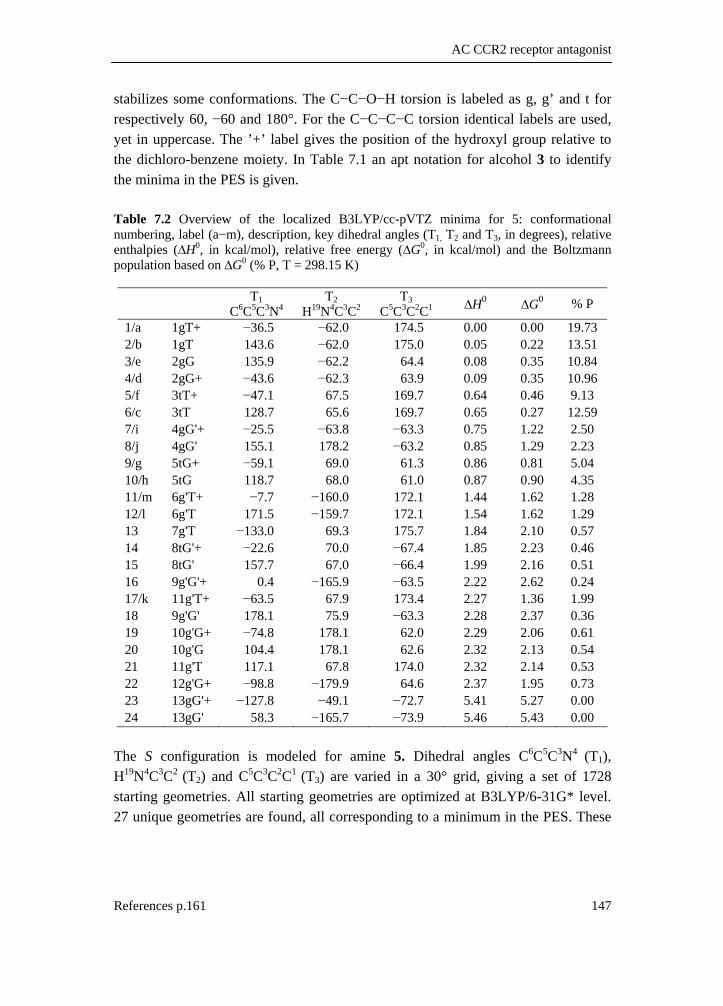
AC CCR2 receptor antagonist
References p.161 147
stabilizes some conformations. The C−C−O−H torsion is labeled as g, g’ and t for respectively 60, −60 and 180°. For the C−C−C−C torsion identical labels are used, yet in uppercase. The ’+’ label gives the position of the hydroxyl group relative to the dichloro-benzene moiety. In Table 7.1 an apt notation for alcohol 3 to identify the minima in the PES is given. Table 7.2 Overview of the localized B3LYP/cc-pVTZ minima for 5: conformational numbering, label (a−m), description, key dihedral angles (T1, T2 and T3, in degrees), relative enthalpies (∆H0, in kcal/mol), relative free energy (∆G0, in kcal/mol) and the Boltzmann population based on ∆G0 (% P, T = 298.15 K)
T1 C6C5C3N4
T2 H19N4C3C2
T3 C5C3C2C1 ∆H0 ∆G0 % P
1/a 1gT+ −36.5 −62.0 174.5 0.00 0.00 19.73 2/b 1gT 143.6 −62.0 175.0 0.05 0.22 13.51 3/e 2gG 135.9 −62.2 64.4 0.08 0.35 10.84 4/d 2gG+ −43.6 −62.3 63.9 0.09 0.35 10.96 5/f 3tT+ −47.1 67.5 169.7 0.64 0.46 9.13 6/c 3tT 128.7 65.6 169.7 0.65 0.27 12.59 7/i 4gG'+ −25.5 −63.8 −63.3 0.75 1.22 2.50 8/j 4gG' 155.1 178.2 −63.2 0.85 1.29 2.23 9/g 5tG+ −59.1 69.0 61.3 0.86 0.81 5.04 10/h 5tG 118.7 68.0 61.0 0.87 0.90 4.35 11/m 6g'T+ −7.7 −160.0 172.1 1.44 1.62 1.28 12/l 6g'T 171.5 −159.7 172.1 1.54 1.62 1.29 13 7g'T −133.0 69.3 175.7 1.84 2.10 0.57 14 8tG'+ −22.6 70.0 −67.4 1.85 2.23 0.46 15 8tG' 157.7 67.0 −66.4 1.99 2.16 0.51 16 9g'G'+ 0.4 −165.9 −63.5 2.22 2.62 0.24 17/k 11g'T+ −63.5 67.9 173.4 2.27 1.36 1.99 18 9g'G' 178.1 75.9 −63.3 2.28 2.37 0.36 19 10g'G+ −74.8 178.1 62.0 2.29 2.06 0.61 20 10g'G 104.4 178.1 62.6 2.32 2.13 0.54 21 11g'T 117.1 67.8 174.0 2.32 2.14 0.53 22 12g'G+ −98.8 −179.9 64.6 2.37 1.95 0.73 23 13gG'+ −127.8 −49.1 −72.7 5.41 5.27 0.00 24 13gG' 58.3 −165.7 −73.9 5.46 5.43 0.00
The S configuration is modeled for amine 5. Dihedral angles C6C5C3N4 (T1), H19N4C3C2 (T2) and C5C3C2C1 (T3) are varied in a 30° grid, giving a set of 1728 starting geometries. All starting geometries are optimized at B3LYP/6-31G* level. 27 unique geometries are found, all corresponding to a minimum in the PES. These

Chapter 7
148
geometries were further optimized at B3LYP/cc-pVTZ level of theory. Four 6-31G* higher energy minima (at least 2.54 kcal/mol above global minimum) could not be located on the cc-pVTZ PES. The essential geometric parameters for the located minima are shown in Table 7.2 along with the relative enthalpy and free energy. To identify all minima, the same notation is used as for compound 3. Some conformations of compound 5 are intramolecularly stabilized through interaction between the N lone pair and the ortho-hydrogens (H21/23). There is also indication for a weaker NH···π interaction. 7.2.8 IR and VCD data
Dipole and rotational strengths are calculated via DFT. The discrete line spectra are broadened using Lorentzian shapes with a full width at half maximum of 10 cm−1 and converted to molar absorptivity units using Equation (7.1) and (7.2).36 As, for the compounds studied, different conformations coexist, the contributions of each conformation have to be taken into account. A Boltzmann weighed distribution is applied to determine the population of each minimum, using relative free energies. In Figures 7.2, 7.3, 7.4 and 7.5 (ii), the simulated IR and VCD spectra are shown i.e. broadened and Boltzmann weighed over all conformations. The calculated frequencies are scaled with a factor 0.98, to correct for the overestimation of the calculated frequencies.37,38 Agreement between experimental and theoretical IR and VCD spectra allows the determination of the absolute configuration of the experimental sample. However, simple comparison is not enough to determine an absolute configuration, and a more thorough analysis of the available data has to be performed. First of all, the different fundamentals need to be assigned in the experimental spectra based on the theoretical data. As VCD is a differential form of IR spectroscopy, IR and VCD transition frequencies are the same. Because of the differential intensities, VCD spectra have extra discriminating potential. As a result, assignment of unresolved IR bands can be performed using the experimental VCD counterpart. Vice versa, assignment of unresolved VCD bands can sometimes be based on IR information. The next step is to determine the experimental dipole and rotational strengths. Here, the assumption is made that the shape of the experimental bands is Lorentzian. The area under the bands can be related to their dipole and rotational strengths.39 Using a Lorentzian peak fitting procedure27, and applying Equations (7.1) and (7.2) the experimental dipole and rotational strengths can be approximated.

AC CCR2 receptor antagonist
References p.161 149
39
39
,max
9.184 10
19.184 10
i i
ii
dD
d
νε
ν
ε νν
−
−
= ⋅
≈ ⋅
∫
∫ (7.1)
39
39
,max
2.296 10
12.296 10
i i
ii
dR
d
νε
ν
ε νν
−
−
= ⋅ Δ
≈ ⋅ Δ
∫
∫ (7.2)
In Equations (7.1) and (7.2), νi,max is the frequency (in cm−1) where the fitted Lorentzian i is centered. Here, ε and Δε are respectively the molar absorptivity and differential molar absorptivity in l.mol−1cm−1. D and R are in esu2cm2. In Tables 7.3, 7.4, 7.5 and 7.6 experimental values for D and R are given with corresponding frequency. The theoretical D and R values in these tables are summed contributions from different conformations. The theoretical frequencies are averaged. In Supplementary Material, tables are given in which the contribution of the significant fundamentals are explicitly reported. 7.3 Results and discussion
The assignment of the fundamentals for compound 3 is not straightforward due to the fact that the contributions of 10 different conformations can be observed. These conformations are situated in a 1.70 kcal/mol energy window (Table 7.1). The main features of the spectra can be explained in terms of the conformations within 1.01 kcal/mol, i.e. 1gT+ (a), 1gT (b), 2gG'+ (c), 2gG' (d), 4tT+ (e) and 4tT (f). Taking into account conformations 3gG (g), 3gG+ (h), 6tG' (i) and 5g'T+ (j) allows the assignment of some small bands in the VCD spectrum. In Figures 7.2 and 7.3 the Lorentzian fitted experimental IR and VCD spectra of (+)-3 are given. In these figures the simulated spectra of (R)-3 also can be found.
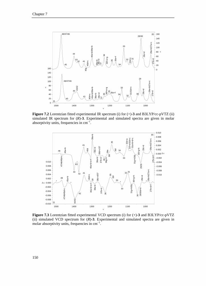
Chapter 7
150
1500 1400 1300 1200 1100 10000
20
40
60
80
100
120
140
160
43/4
2
27b+
d28a+
b/27
a+c
28c+
d
29
30
33
32
31/3
2d+c
3435e+f35
36f+
e+g
363738
c+d
38a+
b
ν
ε
48/47/46
45
44
41
40d+
c40
a+b/
39a+
b
(i)
0
20
40
60
80
100
120
140
160
40g
4232
ε
27b+
d28
a+b/
27a+
c
28c+
d
29/30
33
32d+
c 31
34
35e+
f
35
36f+
e+g
36
3738c+
d38
a+b
48/47/46
45
44
4341
40d+
c
40a+
b/39
a+b
(ii)
Figure 7.2 Lorentzian fitted experimental IR spectrum (i) for (+)-3 and B3LYP/cc-pVTZ (ii) simulated IR spectrum for (R)-3. Experimental and simulated spectra are given in molar absorptivity units, frequencies in cm−1.
1500 1400 1300 1200 1100 1000-0.010
-0.008
-0.006
-0.004
-0.002
0.000
0.002
0.004
0.006
0.008
0.010
* **
47/4
6/45
d+c
ν
Δ ε*
-0.010
-0.008
-0.006
-0.004
-0.002
0.000
0.002
0.004
0.006
0.008
0.010
31f+
e/32
d+c
(i)
36e
36f
36
39c+
d
43
29/3
0d+b
30i+
g+h
40a+
b+e+
f
Δ ε
31g+
h/30
j
27b+
d+f
28a+
b/27
a+c
28c+
d
30
33
32 31
34
35f35
3637b+
d
38c+
d/37
38a+
b
48
45a+
b
42
44/4
3
41
40d+
c
39
47/4
6/45
d+c
30i+
g+h
40a+
b+e+
f
31g+
h/30
j
27b+
d+f
28a+
b/27
a+c
28c+
d29
/30
33
32b+
a
31a+
b+d+
c
3435f
35
36g+
h
37b+
d38
d+c/
3738
a+b
48
45a+
b
4244
41
40d
39a+
b (ii)
Figure 7.3 Lorentzian fitted experimental VCD spectrum (i) for (+)-3 and B3LYP/cc-pVTZ (ii) simulated VCD spectrum for (R)-3. Experimental and simulated spectra are given in molar absorptivity units, frequencies in cm−1.

AC CCR2 receptor antagonist
References p.161 151
The fundamentals corresponding to different conformations are designated using characters (a, b c, etc.) that can be found in Table 7.1. If for two or more conformations the fundamentals coincide or have a small frequency separation, the conformational labels are not given. The small negative and positive shoulders between bands 29/30 and 31 (Figure 7.3) can be attributed to fundamentals 31gh and 30j for the negative one, and 30igh for the positive. The presence of peaks due to these rather high energy conformations can be attributed to the large rotational strengths for a number of fundamentals. In Tables 7.3 and 7.4 the experimental and B3LYP/cc-pVTZ values of D and R are lined up, with their associated frequencies. These tables are a reduced version of the tables that can be found in Supplementary Material. The theoretical frequencies in these tables are averaged over all the pertinent fundamentals. The predicted IR and VCD frequencies are identical, but when comparing the calculated frequencies in Tables 7.3 and 7.4 for identical bands these can be different. This can be explained by the fact that, in these cases, different fundamentals are taken into account. For example, based on the calculated IR data, fundamentals 27/28baef have a predicted B3LYP/cc-pVTZ averaged frequency of 968 cm−1 (Table 7.3). The rotational strengths for fundamentals 27bfd and 27cae/28baef are opposite in sign however (Table 7.4), and can therefore be discerned from each other. In Table 7.4, the calculated frequencies for these two bands (27bfd and 27cae/28baef) are consequently given separately, i.e. 959 cm−1 and 972 cm−1.

Chapter 7
152
Table 7.3 For compound 3: Lorentzian fitted experimental and broadened B3LYP/cc-pVTZ IR frequencies (υ, in cm−1) and dipole strengths (D, in 10−40 esu2cm2) taking into account the fundamentals of 6 lowest energy minima*1 (a–f)
Experiment B3LYP/cc-pVTZ Fundamental υ D υ *2 D*3
27/28baef 969.92 29.81 967.96 95.70 978.31 67.55 28dc 1014.15 73.00 1011.37 44.24 29/30+30ighj 1031.30 105.69 1028.89 197.97 1044.81 40.24 31/32dc 1084.61 43.44 1082.07 65.48 32bafge 1100.34 49.88 1107.12 43.14 33 1132.22 65.31 1121.41 101.35 34 1142.57 32.03 1143.98 8.58 35+35ij 1186.36 22.53 1180.94 75.16 1196.02 45.66 1207.46 47.86 36+36gh 1218.88 26.91 1224.44 72.56 1231.12 37.56 37/38cd 1247.72 9.06 1257.99 26.04 1261.07 26.75 38feab/39dc 1279.31 15.60 1273.65 17.14 39efba/40ebaf 1299.34 23.14 1299.22 71.28 40dc 1315.95 8.10 1324.38 6.18 40hg/41 1343.28 39.69 1342.67 31.54 42/43 1384.81 104.44 1381.81 42.48 44 1402.56 60.50 1402.81 57.31 45/46/47/48 1461.03 43.83 1469.54 160.88 1468.77 128.65 *1 higher energy minima that are used are explicitly mentioned (g,h,i and j) *2 averaged frequencies over the appropriate fundamentals, scaled with factor 0.98 *3 summed over the appropriate fundamentals

AC CCR2 receptor antagonist
References p.161 153
Table 7.4 For compound 3: Lorentzian fitted experimental and broadened B3LYP/cc-pVTZ VCD frequencies (υ, in cm−1) and rotational strengths (R, in 10−44 esu2cm2) taking into account the fundamentals of 6 lowest energy minima*1 (a–f).
Experiment B3LYP/cc-pVTZ Fundamental υ R υ *2 R*3
27bfd 973.22 −2.58 959.00 −1.35 27cae/28baef 981.54 3.29 971.80 4.79 28dc 1020.41 6.91 1011.37 5.38 29/30dcbafe 1030.27 −6.94 1026.38 −18.68 1046.54 −22.22 30igh 1065.66 1.82 1035.20 1.52 30j/31gh 1082.45 −8.73 1052.44 −1.72 31/32+32g 1096.68 21.05 1091.71 26.19 1105.69 10.94 33 1131.37 −10.43 1121.41 −4.76 34 1158.96 2.22 1143.98 2.26 35+35ij 1188.29 7.09 1180.94 16.27 1198.46 14.49 36+36gh 1225.62 −27.60 1224.44 −7.95 37bd 1248.71 −5.09 1251.33 −4.15 37fcae/38cd 1266.90 5.03 1260.20 0.65 38feab 1282.73 −0.35 1269.56 −2.16 1286.56 −1.44 39 1295.85 2.57 1289.82 22.81 40ebaf 1302.87 −1.48 1304.63 −12.27 40dc 1315.13 6.36 1324.38 2.48 40hg/41 1343.87 20.83 1342.67 9.08 42 1369.39 −17.13 1374.30 −32.81 43/44 1385.27 −5.37 1396.06 −25.43 1397.21 −50.56 45eabf 1436.67 3.51 1450.73 0.40 45dc/46/47 1446.92 −4.74 1470.20 −2.10 1457.68 −7.44 48 1468.83 6.25 1480.56 1.73 *1 higher energy minima that are used are explicitly mentioned (g,h,i and j) *2 averaged frequencies over the appropriate fundamentals, scaled with factor 0.98. *3 summed over the appropriate fundamentals
Based on the IR assignment (Table 7.3), the frequencies are predicted with a maximum error of 15 cm−1. The VCD bands can be localized more accurately, due

Chapter 7
154
to the extra discriminating power via the negative and positive intensities. Based on the frequency agreement for the VCD fundamental assignment (Table 7.4) a larger frequency error of maximum 30 cm−1 is therefore observed. For example, fundamental 48 is unresolved in the IR spectrum, and is observed as one band simultaneously with fundamental 47, 46 and 45. In the VCD spectrum, fundamental 48 is clearly resolved, with its predicted frequency overestimated by 12 cm−1. The error that can be observed for the predicted frequencies, even after scaling with a factor 0.98, can be ascribed to the harmonic approximation and the finite basis sets that are used in the calculations.37,38 The relative IR intensities of band 44 and 43/42 are different than predicted, and the intensity of the 40ab/39ab is seriously overestimated. Inspection of the VCD of compound 3 (Figure 7.3) shows that the VCD intensities for fundamentals 40abef and 39 are overestimated. This is due to conformations 1gT+ (a) and 1gT (b) that have a predicted contribution that is clearly too large. Tables 7.3 and 7.4 allow quantitative comparison of the dipole and rotational strengths, in addition to the visual evaluation. From this table it can be seen that the predicted dipole strength for fundamentals 42/43 and 34 are seriously underestimated. The rotational strengths for fundamentals 30j/31gh, 36, 37fcae/38cd, 45dc/46/47 are clearly underestimated, and for fundamental 39 overestimated. More important, no fundamental is predicted with a wrong sign compared to the experiment.
0 50 100 150 2000
50
100
150
200(a)
Dth
eo
Dexp
r2=0.68
-40 -30 -20 -10 0 10 20 30 40
-40
-30
-20
-10
0
10
20
30
40(b)
r2=0.66
Rexp
Rtheo
Figure 7.4 Correlation plot for theoretical (for (R)-3) versus experimental (for (+)-3) (a) dipole strengths (D, in 10−40 esu2cm2) and (b) rotational strengths (R, in 10−44 esu2cm2). Correlation coefficients r2 are given. The blue dotted line has a slope of +1 and intercept of 0.0.

AC CCR2 receptor antagonist
References p.161 155
The correlation coefficients for the dipole and rotational strengths are respectively 0.68 and 0.66 (correlation plots are given in Figure 7.4). These values are acceptable. However, three fundamentals could be identified (39, 40abef and 42) which lower the correlation coefficient drastically for both dipole and rotational strengths. If these fundamentals are taken out, correlation coefficients of 0.81 and 0.91 are obtained for respectively dipole and rotational strength. The difference in experimental and theoretical values for these selected fundamentals could be due to intermolecular association, but no evidence for this was found as the normal modes of these fundamentals could not be related to such interactions. Based on the agreement between experimental and simulated data, and taking into account that the R enantiomer is modeled, it can be concluded that the absolute configuration of (+)-3 can be assigned as (R)-3 in agreement with the proposed configuration. For compound 5, the assignment of fundamentals is even more complex than for the previous compound. Fundamentals from 13 minima can be recognized, all situated within 1.62 kcal/mol interval relative to the global minimum (Table 7.2). The majority of the experimental bands can be explained by the lowest 8 energy conformations, i.e. 1gT+ (a), 1gT (b), 3tT (c), 2gG+ (d), 2gG (e), 3tT+ (f), 5tG+ (g) and 5tG (h). These minima are within a 0.90 kcal/mol energy window. In the IR spectrum (Figure 7.5) one band (37klm) can only be explained by taking conformations 11g'T+ (k), 6g'T (l) and 6g'T+ (m) into account. Also conformations 4gG'+ (i) and 4gG' (j) have a considerable contribution. Again, in the region 1200–1400 cm−1 the number of fundamentals is very high and IR intensities are low, which complicates their assignment. The maximum error for the predicted frequencies based on the IR results is 13 cm−1, and 16 cm−1 based on the VCD results. It can also be seen in Figure 7.4 and 7.5 that scaling with 0.98 gives better agreement with experiment than for compound 3. The negative shoulder in the experimental spectrum at 1277 cm−1 can not be assigned based on the simulated spectrum. Though, when examining the extended table (in Supplementary Material) it can be seen that fundamentals 40g and 40h have small negative intensities, and are centered at 1284 and 1286 cm−1 respectively. Therefore this negative shoulder at 1277 cm−1 is assigned as 40gh.

Chapter 7
156
1500 1400 1300 1200 1100 10000
102030405060708090
100110120130140150160170
32c
36
(ii)
49/4
8/47
/46
46a+
b
45
44
4241
h/g
40c+
f/41
38e+
b/39
38 37k+
l+m
34/3
3b+f
+c
33a+
g+h
ν
ε
(i)
31/3
0/29
d+e
3233d+
e
35
36
37
39a+
b/4043
46a+
b
45
44 42
41h/
g
40c+
f/41
38e+
b/39
38 37k+
l+m
34/3
3b+f
+c
33a+
g+h
31/3
0/29
d+e
32c+
f+h+
g
32e+
b+d+
a
33d+
e
35
36i+
j
3739a+
b/40
43
0
20
40
60
80
100
120
140
160
ε
Figure 7.5 Lorentzian fitted experimental IR spectrum (i) for (−)-5 and B3LYP/cc-pVTZ (ii) simulated IR spectrum for (S)-5. Experimental and simulated spectra are given in molar absorptivity units, frequencies in cm−1.
1500 1400 1300 1200 1100 1000-0.010
-0.008
-0.006
-0.004
-0.002
0.000
0.002
0.004
0.006
(ii)
36i+
j
49
48/4
7
46
43
37a+
b
31
ν
Δ ε
46a+
b
45
44
42
40g+
h
38/3
9/40
37c+
h+g+
f
34/3
3c
33
(i)
31/3
0/29
d+e
32
33d+
e
35
36
37d+
e
41/4
0f+c
-0.010
-0.008
-0.006
-0.004
-0.002
0.000
0.002
0.004
0.006
43e+
d+a+
b
41g+
h 41 39a+
b/40
e+d
40f+
c 38e+
b/39
3232
g+h
Δ ε
49
48/4
7
46
43 37a+
b
3146a+
b
45
44
42
40g+
h+b+
a
38
37c+
h+g+
f
34/3
3c
33
31c+
f/30/
29d+
e
32c+
f
33d+
e
35
36
37d+
e
41f+
c
43e+
d+a+
b
Figure 7.6 Lorentzian fitted experimental VCD spectrum (i) for (−)-5 and B3LYP/cc-pVTZ (ii) simulated VCD spectrum for (S)-5. Experimental and simulated spectra are given in molar absorptivity units, frequencies in cm−1.

AC CCR2 receptor antagonist
References p.161 157
Table 7.5 For compound 5: Lorentzian fitted experimental and broadened B3LYP/cc-pVTZ IR frequencies (υ, in cm−1) and dipole strengths (D, in 10−40 esu2cm2) taking into account the fundamentals of 8 lowest energy minima*1 (a–h)
Experiment B3LYP/cc-pVTZ Fundamental υ D*2 υ D*3
29de/30/31 1029.22 97.97 1024.61 107.81 1044.73 5.52 32 1056.28 7.84 1061.99 25.56 1072.63 7.56 33de 1093.60 10.40 1091.57 5.14 33hga 1105.71 14.29 1102.11 15.16 33bfc/34 1131.34 78.38 1119.38 120.58 35 1142.15 28.37 1143.28 16.11 36 1184.90 27.23 1179.86 43.54 37klm 1207.97 12.77 1198.75 2.93 37 1218.68 10.17 1217.53 11.20 38hgfcad 1247.86 4.31 1249.92 11.32 38eb/39gcdhef 1258.61 8.36 1262.38 8.46 39ab/40edbagh 1276.45 7.39 1281.24 10.32 40fc/41cfdeab 1301.97 1.51 1307.17 10.60 41hg 1319.07 2.00 1328.02 5.31 42 1338.42 11.38 1346.34 22.02 1345.05 13.85 43+43lkm 1356.26 10.95 1367.88 27.96 1362.91 17.92 44 1381.79 20.21 1388.58 9.12 45 1397.58 52.24 1405.92 60.86 1404.76 37.56 46ab 1448.49 1.37 1452.79 1.18 46fcdegh/47/48/49 1458.79 15.05 1471.32 174.67 1467.59 186.74 1485.27 2.98 *1 higher energy minima that are used are explicitly mentioned (k,l and m) *2 averaged frequencies over the appropriate fundamentals, scaled with factor 0.98. *3 summed over the appropriate fundamentals

Chapter 7
158
Table 7.6 For compound 5: Lorentzian fitted experimental and broadened B3LYP/cc-pVTZ VCD frequencies (υ, in cm−1) and rotational strengths (R, in 10−44 esu2cm2) taking into account the fundamentals of 6 lowest energy minima*1 (a–h)
Experiment B3LYP/cc-pVTZ Fundamental υ R υ *2 R*3
29de/30/31cf 1027.08 −12.03 1022.40 −6.24 31adbghe 1044.31 8.56 1029.02 1.94 32 1058.06 1.84 1061.99 −2.52 1069.71 −3.31 1079.42 −3.07 33ed 1089.42 3.29 1091.57 3.14 1094.95 4.70 33ghabf 1106.33 −4.92 1105.93 −5.73 33c/34 1121.67 4.15 1121.09 4.79 1128.72 5.78 35 1140.08 −5.96 1143.28 −3.66 36 1182.17 −15.89 1179.86 −22.44 1190.99 −5.08 37hcgf 1209.91 10.54 1213.17 6.02 37ab 1220.39 −1.89 1219.20 −2.51 37de 1228.71 2.75 1224.57 1.28 38/39/40edba 1246.23 −1.18 1263.95 17.47 1249.31 8.50 1255.82 11.88 40gh 1276.65 −2.81 1284.76 −0.25 40fc/41 1288.58 4.96 1311.34 8.72 1301.71 7.33 42 1343.57 −36.50 1346.34 −23.36 43edab 1357.01 5.27 1364.00 4.72 43fgch+43lkm 1373.47 −6.24 1370.10 −6.36 44 1383.72 3.92 1388.58 2.10 45 1395.96 5.05 1405.92 18.11 1401.30 14.91 46ab 1438.10 −2.30 1452.79 0.09 46fcdegh/47fc 1448.25 2.30 1461.76 1.29 47bdag/48 1463.52 2.02 1471.86 1.32 49 1468.95 −4.21 1479.94 −1.29 1482.76 −2.05 *1 higher energy minima that are used are explicitly mentioned (k,l and m) *2 averaged frequencies over the appropriate fundamentals, scaled with factor 0.98. *3 summed over the appropriate fundamentals

AC CCR2 receptor antagonist
References p.161 159
The rotational strengths of fundamentals 46a and 46b are respectively 0.61 and −0.52 and are centered at 1453 cm−1. Their sum is positive and consequently its sign does not agree with the experimental observation as is shown in Table 7.6 and can be seen in Figure 7.6. The signs of the rotational strengths vary for the different conformations for fundamental 32 as can be seen in Figure 7.6 and the extended table in Supplementary Material. In the experimental spectrum, the band assigned as fundamental 32 is not resolved and has a negative sign. Summing over all the rotational strengths for the significant conformations (a–h) for fundamental 32, this value also appears to be negative in agreement with experiment, as can be seen in Table 7.6. Further, dipole strengths for fundamentals 37klm and 40 are underestimated, and for fundamentals 40fc/41cfdeab they are overestimated. The rotational strength for fundamental 31adbghe is found to be underestimated.
0 50 100 150 2000
20
40
60
80
100
120
140
160
180
200
Dth
eo
Dexp
r2=0.91
-40 -30 -20 -10 0 10 20
-40
-30
-20
-10
0
10
20(b)(a)
r2=0.92
Rexp
Rtheo
Figure 7.7 Correlation plot for theoretical (for (S)-5) versus experimental (for (−)-5) (a) dipole strength (D, in 10−40 esu2cm2) and (b) rotational strengths (R, 10−44 esu2cm2). Correlation coefficients r2 are given. The blue dotted line has a slope of +1 and an intercept of 0.0. The correlation coefficients between theoretical and experimental values of D en R are 0.91 for the dipole strengths and 0.92 for the rotational strengths, which is excellent (Figure 7.7). Given the good agreement between experimental and theoretical data, and taking into account that the S enantiomer is modeled, the absolute configuration of (−)-5 can be assigned to (S)-5, in agreement with the proposed configuration.
Chapter 7
160
7.4 Conclusion
In this study the absolute configurations for two related compounds (+)-3 and (−)-5 are determined with success. Both are successive precursors of JNJ-27553292 (−)-1, a CCR2 receptor antagonist. The absolute configurations for both (+)-3 and (−)-5 were proposed based on a reaction performed on a similar compound, and were found to be in agreement with absolute configurations based on the VCD determination. Starting with the prochiral 3,4-dichlorobenzaldehyde, using the N,N'-((1S,2S)-cyclohexane-1,2-diyl)bis(trifluoromethanesulfonamide) catalyst it could be determined that (+)-(R)-3 is formed and consequently (−)-(S)-5. Further, using (−)-(S)-5 to synthesize (−)-1, no racemization occurs, which means that based on the reaction mechanism shown in Scheme 7.1, the absolute configuration of the active enantiomer of 1 can be assigned to be (−)-(S)-1 7.5 Supplementary material index
For this chapter Supplementary Material is provided. It can be downloaded from http://www.quantum.UGent.be/tksup.pdf Table S7.1 For compound 3: Experimental Lorentzian fitted and B3LYP/cc-pVTZ vibrational frequencies, dipole strengths and rotational strengths taking into account the fundamentals of the 10 lowest energy minima (a–j). Table S7.2 For compound 5: Experimental Lorentzian fitted and B3LYP/cc-pVTZ IR frequencies, dipole strengths and rotational strengths taken into account the fundamentals of the 13 lowest energy minima (a–m). Figure S7.1 Pictorial representation of the most contributing B3LYP/cc-pVTZ PES minima for (R)-3. Figure S7.2 representation of most contributing B3LYP/cc-pVTZ PES minima for (S)-5

AC CCR2 receptor antagonist
161
7.6 Reference list
1. Dawson, J.; Miltz, W.; Mir, A. K.; Wiessner, C. Expert Opin. Ther. Targets
2003, 7, 35-48.
2. Van Lommen, G.; Doyon, J.; Coesemans, E.; Boeckx, S.; Cools, M.; Buntinx, M.; Hermans, B.; VanWauwe, J. Bioorg. Med. Chem. Lett. 2005, 15, 497-500.
3. Boeckx, G. M.; Van Lommen, G.; Doyon, J.; Coesemans, E. WO 2005118574, 2005.
4. Boeckx, G. M.; Van Lommen, G.; Doyon, J.; Coesemans, E. WO 2005118578, 2005.
5. Van Lommen, G.; Doyon, J.; Van Wauwe, J. P.; Cools, M.; Coesemans, E. WO 2004069809, 2003.
6. Thompson, A. S.; Humphrey, G. R.; Demarco, A. M.; Mathre, D. J.; Grabowski, E. J. J. J. Org. Chem. 1993, 58, 5886-5888.
7. Yoshioka, M.; Kawakita, T.; Ohno, M. Tetrahedron Lett. 1989, 30, 1657-1660.
8. Kitamura, M.; Suga, S.; Kawai, K.; Noyori, R. J. Am. Chem. Soc. 1986, 108, 6071-6072.
9. Stephens, P. J.; Devlin, F. J. Chirality 2000, 12, 172-179.
10. Stephens, P. J. Vibrational circular dichroism spectroscopy: A new tool for the stereochemical characterization of chiral molecules. In Computational medicinal chemistry for drugs discovery, Bultinck, P., De Winter, H., Langenaeker, W., Tollenaere, J. P., Eds.; Marcel Dekker, Inc.: New York, 2004; pp 699-725.
11. Berova, N.; Nakanishi, K.; Woody, R. W. Circular Dichroism: Principles and Applications; 2nd ed.; Wiley-VCH: New York, 2000.
12. Holzwart, G.; Hsu, E. C.; Mosher, H. S.; Faulkner, T. R.; Moscowit, A. J. Am. Chem. Soc. 1974, 96, 251-252.
13. Nafie, L. A.; Keiderling, T. A.; Stephens, P. J. J. Am. Chem. Soc. 1976, 98, 2715-2723.

Chapter 7
162
14. Freedman, T. B.; Cao, X. L.; Dukor, R. K.; Nafie, L. A. Chirality 2003, 15, 743-758.
15. Cheeseman, J. R.; Frisch, M. J.; Devlin, F. J.; Stephens, P. J. Chem. Phys. Lett. 1996, 252, 211-220.
16. Devlin, F. J.; Stephens, P. J.; Cheeseman, J. R.; Frisch, M. J. J. Phys. Chem. A 1997, 101, 9912-9924.
17. Stephens, P. J.; Devlin, F. J.; Chabalowski, C. F.; Frisch, M. J. J. Phys. Chem.-US 1994, 98, 11623-11627.
18. Ayers, P. W.; Yang, W. Density-functional theory. In Computational medicinal chemistry for drugs discovery, Bultinck, P., De Winter, H., Langenaeker, W., Tollenaere, J. P., Eds.; Marcel Dekker, Inc.: New York, 2004; pp 89-118.
19. Kuppens, T.; Bultinck, P.; Langenaeker, W. Drug Discovery Today: Techn. 2004, 1, 269-275.
20. Urbanova, M.; Setnicka, V.; Volka, K. Chirality 2000, 12, 199-203.
21. Nafie, L. A. Appl. Spectrosc. 2000, 54, 1634-1645.
22. Kuppens, T.; Vandyck, K.; Van der Eycken, J.; Herrebout, W.; van der Veken, B. J.; Bultinck, P. J. Org. Chem. 2005, 70, 9103-9114.
23. Setnicka, V.; Urbanova, M.; Bour, P.; Kral, V.; Volka, K. J. Phys. Chem. A 2001, 105, 8931-8938.
24. Frisch, M. J.; Trucks, G. W.; Schlegel, H. B.; Scuseria, G. E.; Robb, M. A.; Cheeseman, J. R.; Montgomery Jr, J. A.; Vreven, T.; Kudin, K. N.; Burant, J. C.; Millam, J. M.; Iyengar, S. S.; Tomasi, J.; Barone, V.; Mennucci, B.; Cossi, M.; Scalmani, G.; Rega, N.; Petersson, G. A.; Nakatsuji, H.; Hada, M.; Ehara, M.; Toyota, K.; Fukuda, R.; Hasegawa, J.; Ishida, M.; Nakajima, T.; Honda, Y.; Kitao, O.; Nakai, H.; Klene, M.; Li, X.; Knox, J. E.; Hratchian, H. P.; Cross, J. B.; Bakken, V.; Adamo, C.; Jaramillo, J.; Gomperts, R.; Stratmann, R. E.; Yazyev, O.; Austin, A. J.; Cammi, R.; Pomelli, C.; Ochterski, J. W.; Ayala, P. Y.; Morokuma, K.; Voth, G. A.; Salvador, P.; Dannenberg, J. J.; Zakrzewski, V. G.; Dapprich, S.; Daniels, A. D.; Strain, M. C.; Farkas, O.; Malick, D. K.; Rabuck, A. D.; Raghavachari, K.; Foresman, J. B.; Ortiz, J. V.; Cui, Q.; Baboul, A. G.; Clifford, S.; Cioslowski, J.; Stefanov, B. B.; Liu, G.; Liashenko, A.; Piskorz, P.; Komaromi, I.; Martin, R. L.; Fox, D. J.; Keith, T.; Al-Laham, M. A.; Peng, C. Y.; Nanayakkara, A.; Challacombe, M.; Gill, P.

AC CCR2 receptor antagonist
163
M. W.; Johnson, B.; Chen, W.; Wong, M. W.; Gonzalez, C.; Pople, J. A. Gaussian03, Revision B5; Gaussian, Inc.: Wallingford CT, 2004.
25. Becke, A. D. J. Chem. Phys. 1993, 98, 5648-5652.
26. Lee, C. T.; Yang, W. T.; Parr, R. G. Phys. Rev. B-Condens. Matter 1988, 37, 785-789.
27. Kuppens, T.; Langenaeker, W.; Tollenaere, J. P.; Bultinck, P. J. Phys. Chem. A 2003, 107, 542-553.
28. Hehre, W. J.; Radom, L.; Schleyer, P. R.; Pople, J. A. Ab initio molecular orbital theory; Wiley: 1986.
29. Sadowski, J.; Schwab, C. H.; Gasteiger, J. 3D structure generation and conformational searching. In Computational medicinal chemistry for drugs discovery, Bultinck, P., De Winter, H., Langenaeker, W., Tollenaere, J. P., Eds.; Marcel Dekker, Inc.: New York, 2004; pp 151-212.
30. Woon, D. E.; Dunning, T. H. J. Chem. Phys. 1993, 98, 1358-1371.
31. Kendall, R. A.; Dunning, T. H.; Harrison, R. J. J. Chem. Phys. 1992, 96, 6796-6806.
32. Ditchfield, R. Mol. Phys. 1974, 27, 789-807.
33. Stephens, P. J. J. Phys. Chem.-US 1987, 91, 1712-1715.
34. McQuarrie, D. A. Statistical Thermodynamics; Harper and Row: New York, 1973.
35. Polavarapu, P. L. Spectroscopy 1994, 9, 48-55.
36. Schellman, J. A. Chem. Rev. 1975, 75, 323-331.
37. Wong, M. W. Chem. Phys. Lett. 1996, 256, 391-399.
38. Scott, A. P.; Radom, L. J. Phys. Chem.-US 1996, 100, 16502-16513.
39. Rauk, A. Vibrational circular dichroism Intensities: Ab initio calculations. In New developments in molecular chirality, Mezey, P. G., Ed.; Kluwer academic publishers: 1991; pp 57-92.
References p.220 165
8 self-association behavior of
carboxylic acids in solution:
a VCD perspective
Equation Chapter 8 Section 1 8.1 Introduction
Carboxylic acids are known for their strong intermolecular associations1,2 which can appear in solid, liquid and gas-phase state, but also in solutions. Even in diluted solution, self-association can be observed and, depending on solvent, concurrent association between the solvent and the carboxylic acid moiety can be observed.3 Aggregation can considerably influence the conformational properties of the compound. In solutions with non-polar solvents, solvent-solute interaction can be possible, as was touched upon discussing CDCl3−OH interaction in Chapter 6. These kind of solvent-solute aggregations are not regarded as a general problem, as the spectra, simulated without considering the aggregation, still show a high degree of agreement with experimental spectra. The differences which sometimes can be seen, often can be explained by taking into account the solvent effects. Interaction between carboxylic acids groups are a complete different story. It is generally known that carboxylic acids form strong dimeric complexes which have

Chapter 8
166
complete different conformational properties compared to the monomer form. This implicates that the vibrational properties of monomer and dimer are also completely different, which complicates the simulation of their vibrational spectra. If, for example, the absolute configuration of a chiral carboxylic acid needs to be determined and one results to the analysis of the compound without considering the self-associative behavior, these monomeric spectra will probably show no agreement with experiment. Therefore, no conclusions can be drawn from such a study. A solution to this problem is, to explicitly take into account dimer formation.4 Problems inherent with this approach are the size of the problem, i.e., larger molecular systems, and the need for larger basis sets to correctly describe the hydrogen bonding. In dilute solutions, often an equilibrium between monomer and dimer structures exists which means that the measured spectra can be attributed to both the properties of monomer and dimer structures. It is difficult, however, to asses and determine the equilibrium constant, which complicates the simulation of monomer/dimer spectra considerably. Another approach is to form the corresponding methyl-ester of the carboxylic acid under study. No major intermolecular association will occur for a methyl-ester, compared to the acid.5 If no racemization occurs during the methyl-ester forming reaction, the absolute configuration of the methyl-ester will be correlated to the absolute configuration of the parent carboxylic acid. In this chapter, tetrahydrofuran-2-carboxylic acid is studied and spectra are simulated on the basis of both monomeric and dimeric structures using experimentally determined equilibrium constants. The corresponding methyl-ester is also studied, for which the spectra are simulated using different hybrid density functionals. The absolute configuration determination performed for Johnson & Johnson Pharmaceutical Research and Development on tetrahydrofuran-3-carboxylic acid is also described in this chapter.

Carboxylic acids – VCD perspective
References p.220 167
8.2 Intermolecular association of tetrahydrofuran-2-carboxylic
acid in solution: a vibrational circular dichroism study
8.2.1 Introduction
In this study tetrahydrofuran-2-carboxylic acid 1 is studied using vibrational spectroscopy including both unpolarized infrared (IR) and vibrational circular dichroism (VCD) spectroscopy. (R)-tetrahydrofuran-2-carboxylic acid is a chiral building block for faropenem (7-(1-hydroxyethyl)-6-oxo-3-oxolan-2-yl-2-thia-5-azabicyclo[3.2.0]hept-3-ene-4-carboxylicacid),6,7 a clinically effective nonnatural β-lactam antibiotic.8 In combination with density functional theory (DFT) calculations,9 VCD spectroscopy allows the elucidation of the absolute configuration and the conformational behavior of chiral compounds.10-12 By doing DFT calculations on a compound with known stereochemistry, one can simulate IR and VCD spectra and consequently compare them with experimental spectra. The IR spectra of enantiomers are identical but the VCD spectra, which are in essence differential IR spectra recorded with left and right circularly polarized infrared light, have intensities with opposite sign. As each vibrational transition band has a corresponding VCD band, each one of these bands can be compared with the simulated spectrum, allowing a very reliable assignment of the stereochemistry of the measured enantiomerically pure sample. At the same time, information about the primary conformations is obtained, as VCD is very sensitive to conformational change. The VCD method was proven very successful in the past13-19 and further development in spectroscopic techniques and computational algorithms will further increase the reliability of this method.20,21 1 is a carboxylic acid, and these types of compounds are known to form intermolecular aggregates.1,2 In the solid and liquid phase, associations mainly involve cyclic dimers. These are also formed in the gas phase and in solutions. In protic solvents, hydrogen bonding with solvent molecules appears concurrent to dimer formation.3 As self-association considerably influences the conformational
Kuppens, T.; Herrebout, W.; van der Veken, B. J.; Bultinck, P. J. Phys. Chem. A 2006, 100, 10191-10200.

Chapter 8
168
and vibrational properties of the molecules,22-24 a suitable model has to be used when computing IR and VCD spectra. In the past, only a few studies were carried out on dimers, in which the focus was on relatively rigid structures.25,26 A more recent and extensive paper4 from He et al. describes a VCD study on α-(aryloxy)propanoic acid cyclic dimers; however, the equilibrium between monomer and dimer was not further investigated. Also, recently Urbanová et al.27 published a VCD study concerning a tetrameric dimethylbiphenyldicarboxylic acid structure. In both studies the calculations are performed with the B3LYP hybrid functional using the 6-31G* basis set. In this study the computational level is extended, by means of the use of different functionals and larger basis sets. The focus of the present paper is first to establish whether the dimerization has an important effect on the experimental spectra. Second, it is investigated if this effect can be simulated using DFT calculations. Further, a semiquantitative model is defined to obtain estimates of monomer and dimer populations. Combining the semiquantitative populations and DFT results, the experimental IR and VCD will be assessed. 8.2.2 Experimental methods
(R)-(+)-1 ( α20
D = +30.0 (c = 0.34, CHCl3))6 and (S)-(−)-1 ( α20D = −12.6 (c = 7.70,
H2O)28 were obtained from Acros with a 97.5% ee and were used without further purification. IR spectra are measured with a Bruker Vector 22 FTIR spectrometer. The VCD is measured with an IFS 66v/S FTIR spectrometer coupled to a PMA37 module, set up as described in Urbanová et al.29 Long wave pass filters are used to select an operational frequency window to improve the signal-to-noise (S/N) ratio. Because it can induce large artifacts in the CO stretching region for compound 1, the default 1830 cm−1 filter is unusable. Therefore, a 1960 cm−1 filter is used instead,30 which allows measurement in the CO stretch region. As this filter has a rather high long wave cutoff at 1250 cm−1, the 1830 cm−1 filter is used for the measurements for (R)-(+)-1 and (S)-(−)-1 below 1200 cm−1, using CS2 as solvent and KBr cell windows. Above 1200 cm−1, the 1960 cm−1 filter is used, in combination with CDCl3 as solvent and CaF2 cell windows. The collection time for the VCD spectra is 90 minutes (3x30 minutes) each. The demountable cells are equipped with a 105 µm Teflon spacer. (R)-(+)-1 and (S)-(−)-1 are dissolved in CDCl3 at a concentration of 0.42 M, 0.25 M and 0.21 M. 1 has a low solubility in CS2 and a solution is prepared at an approximate concentration of 0.11 M. Because both enantiomers are available,

Carboxylic acids – VCD perspective
References p.220 169
half-difference spectra31 are computed as ( )/2ε ε− +Δ − Δ , which provides spectra with an improved S/N ratio. An infrared concentration study with (R)-(+)-1 in CHCl3 was performed using a KBr cell with a 200 µm Teflon spacer. 8.2.3 Computational methods
Geometry optimizations and calculations of the dipole strengths (D) and rotational strengths (R) are performed using Gaussian03.32 In this study the B3LYP33,34 hybrid functional is used, which has proven its reliability in the calculation of VCD intensities,16,17,35 and the description of strong hydrogen bonded complexes.36 The potential energy surface for the monomer and dimer are scanned using different methods, which are described in §8.2.4. The located monomer and dimer minima are optimized with the aug-cc-pVTZ basis set. This basis set was previously found capable of describing hydrogen bonded systems.37 Six additional functionals (B1LYP, B3P86, B3PW91, B98, MPW1PW91, PBE1PBE)38 are also employed in combination with the 6-31++G** basis set for which the results can be found in Supplementary Material (Figures S8.3 and S8.4). Hessian matrices, atomic polar tensors (APT) and atomic axial tensors (AAT) are calculated using gauge-including/invariant atomic orbitals (GIAOs),39,40 at the same level as the optimization, allowing the calculation of dipole and rotational strengths. The free energy is calculated under the usual assumptions using standard thermochemical expressions.41 A scaling factor of 0.980 is used to correct for the harmonic approximation.42 The calculations were performed on the Ghent Quantum Cluster at Ghent University and CalcUA located at the University of Antwerp. 8.2.4 Conformational search
The potential energy surfaces of the monomer and dimer of 1 with the S configuration were thoroughly analyzed to find the lower energy minima. For the monomer, a conformational analysis was done using MM343 and MM444 stochastic search methods, for which the implementation is described in more detail in earlier work,16 and a Monte Carlo search using the MMFF45 force field. All unique minima were subsequently optimized on the B3LYP/6-31G* level. A systematic
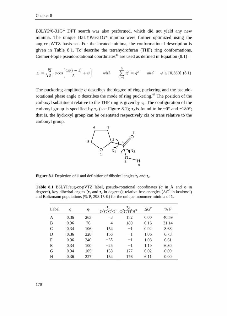
Chapter 8
170
B3LYP/6-31G* DFT search was also performed, which did not yield any new minima. The unique B3LYP/6-31G* minima were further optimized using the aug-cc-pVTZ basis set. For the located minima, the conformational description is given in Table 8.1. To describe the tetrahydrofuran (THF) ring conformations, Cremer-Pople pseudorotational coordinates46 are used as defined in Equation (8.1) :
[ ]5
2 2
1
4 ( 1)2cos 0, 360
5 5i ii
iz q with z q and
πϕ ϕ
=
⎛ − ⎞⎟⎜= ⋅ + = ∈⎟⎜ ⎟⎜⎝ ⎠ ∑ (8.1)
The puckering amplitude q describes the degree of ring puckering and the pseudo-rotational phase angle φ describes the mode of ring puckering.47 The position of the carboxyl substituent relative to the THF ring is given by τ1. The configuration of the carboxyl group is specified by τ2 (see Figure 8.1); τ2 is found to be ~0° and ~180°; that is, the hydroxyl group can be orientated respectively cis or trans relative to the carbonyl group.
O
O
OH
1
2
34
5 6
7
89
τ1 τ2
Figure 8.1 Depiction of 1 and definition of dihedral angles τ1 and τ2 Table 8.1 B3LYP/aug-cc-pVTZ label, pseudo-rotational coordinates (q in Å and φ in degrees), key dihedral angles (τ1 and τ2 in degrees), relative free energies (ΔG0 in kcal/mol) and Boltzmann populations (% P, 298.15 K) for the unique monomer minima of 1.
Label q φ τ1 O8C6C2O1
τ2 O7C6O8H9 ΔG0 % P
A 0.36 263 −3 182 0.00 40.59 B 0.36 76 4 180 0.16 31.14 C 0.34 106 154 −1 0.92 8.63 D 0.36 228 156 −1 1.06 6.73 F 0.36 240 −35 −1 1.08 6.61 E 0.34 100 −25 −1 1.10 6.30 G 0.34 105 153 177 6.02 0.00 H 0.36 227 154 176 6.11 0.00

Carboxylic acids – VCD perspective
References p.220 171
For the dimer of 1, an MM3 and MM4 stochastic search was performed. This search yielded two relatively stable classes of geometries, which are given schematically in Figure 8.2. The most stable dimer is the classical one in which the two carboxylic acid groups form a strong hydrogen bonded association (Figure 8.2a). Cyclic associations are also observed in which the THF oxygen of one monomer is involved in forming cyclic dimers (Figure 8.2b). Noncyclic dimers with only one OH···O hydrogen bond were located as well but were discarded due to their high energy.48 Further optimization at the 6-31++G** level showed that the dimers, in which the THF oxygen is involved, have a relative free energy of at least 5.5 kcal/mol compared to the other more stable carboxylic acid bonded cyclic dimers. Consequently, it can be concluded that, when the dimers are considered, the classic cyclic dimers are most contributing. As the stochastic search did not yield many cyclic dimer geometries, a B3LYP/6-31++G** systematic search was performed in which Τ1 and Τ1’ (the position of the carboxyl substituent relative to THF for the dimers as defined in Figure 8.2) were varied in a 30° grid for different values of q and φ for both THF rings. Using this approach, a total of 10 unique minima was located. These geometries were further optimized at the aug-cc-pVTZ level for which the conformational description is given in Table 8.2.
O
O
H O
H OO
O
O
O
H
O
O
H
O O
T1
T1' a
b
Figure 8.2 Two different possibilities to form cyclic dimers of 1. Definition of dihedral angles Τ1 and Τ1’.
Chapter 8
172
Table 8.2 B3LYP/aug-cc-pVTZ label, symmetry, pseudo-rotational coordinates (q in Å and φ in degrees), key dihedral angles (Τ in degrees), relative enthalpies (ΔH0 in kcal/mol), relative free energies (ΔG0 in kcal/mol) and Boltzmann populations (% P, 298.15 K) for the unique dimer minima of 1.
Label q1 φ1 Τ1
O8C6C2O1 q2 φ2 Τ1’
O8’C6’C2’O1’ ΔH0 ΔG0 % P
DC C1 0.36 232 156 0.34 102 156 0.06 0.00 24.2 FC C1 0.36 237 −35 0.34 108 155 0.12 0.19 17.5 EC C1 0.33 100 −29 0.34 105 156 0.27 0.52 10.1 CC C2 0.34 103 155 0.34 103 155 0.09 0.57 9.3 FD C1 0.36 237 −34 0.36 232 155 0.04 0.58 9.1 FF C2 0.36 238 −37 0.36 238 −37 0.37 0.59 8.9 ED C1 0.34 96 −31 0.36 232 154 0.23 0.63 8.4 FE C1 0.36 240 −36 0.34 105 −26 0.58 0.91 5.2 DD C2 0.36 234 154 0.36 234 154 0.00 0.94 5.0 EE C2 0.34 101 −27 0.34 102 −27 0.75 1.40 2.3
It can be seen that each of these dimers are in fact combinations of monomer geometries, more precisely, the 4 monomers of 1 that have a cis carboxylic acid group configuration (C, D, E and F) and that are conformationally capable of forming cyclic dimers. However, clearly not all monomer geometries for 1 are able to form dimer structures as can be seen in Figure 8.3, as these are intramolecular hydrogen bonded structures in which the trans carboxylic OH interacts with the THF oxygen. There are also two trans carboxylic monomer structures located in which no intramolecular hydrogen bonding is present (conformation G and H in Table 8.1). Because of their high energies these minima are not significant. If the relative enthalpy is compared to the relative free energy of the dimer structures, a different order can be observed. This is due to the various entropy contributions of each dimer minimum, e.g., dimers structures with C2 symmetry have a lower rotational entropy contribution compared to C1 structures.

Carboxylic acids – VCD perspective
References p.220 173
FD
EC
A B
Figure 8.3 Model representations of the monomer conformations A–F and at the same time exemplary models of cyclic dimers EC and FD. 8.2.5 Results and discussion
In Figure 8.4a, the CO stretch region of the IR spectrum is presented for (R)-(+)-1 solutions in CHCl3, with typical concentrations varying between 0.01 and 0.40 M. Two intense bands can be observed in this region, with a rather large frequency separation, which, in the case of carboxylic acids, is often an indication for coexistence of dimer and monomer in solution.49 This is confirmed in the OH stretch region, given in Figure 8.4b, in which two monomer bands can be observed near 3390 and 3500 cm−1 and a broad dimer band near 3000 cm−1. In both the CO and OH stretch region the bands can be identified on the basis of DFT results. In Figure 8.4 the monomer and dimer calculated spectra are concurrently given (Tables S8.4 and S8.5 in Supplementary Material describe the fundamentals for monomer and dimer conformations). From these data it can be seen that band P1 can be assigned to the monomer with conformations A and B and P2 to the cis-configured monomer (C, D, E and F). For conformations A and B, the carbonyl stretch frequency is somewhat higher and the hydroxyl stretch frequency is somewhat lower compared to the non-

Chapter 8
174
hydrogen bonded monomers C, D, E and F. Also, the intensity of the hydrogen bonded monomer bands is higher compared to the cis configured monomers. These findings agree with the B3LYP intensities and populations. Further, band P3 can be ascribed to the dimer conformations in the same manner. The typical concentration dependence of the three bands also confirms the assignment of monomer and dimer bands.
1800 1750 17000
50
100
150
200
250
300
350
400
P3
P3
P2
P2
P134
C+D
+F+E
34A+
B
74 10mM 20mM 40mM 0.1M 0.2M 0.3M 0.4M
ε
ν
P1
74FF+FE+EE
34F+
E
34A+B
74FC+FD+EC+ED
74DC+CC+DD
34C
+D
3800 3600 3400 3200 3000 2800
20
40
60
80
100
120
140
P3
P1
90/89/88
42C+D+E+F
42A+B
10mM 20mM 40mM 0.1M 0.2M 0.3M 0.4M
ε
ν
P3
P1
P2
P241-35
42C+D+E+F
87-75 90/89/88
42A+B
Figure 8.4 IR spectra of (R)-(+)-1 in CHCl3 for different concentrations varying between 0.4 M and 10 mM) in the CO stretch (top) and OH stretch (bottom) region concurrent with the B3LYP/aug-cc-pVTZ simulated spectra for monomer (solid line) and dimer (dotted line) and assignments. Intensities in molar absorptivity units, frequencies in cm−1.

Carboxylic acids – VCD perspective
References p.220 175
Solutions in CS2 are also studied to extend the VCD frequency range. For (R)-(+)-1 in CS2 three carbonyl stretch bands can be observed (Figure S8.1 in Supplementary Material), similar to the CHCl3 spectra: P1 centered at 1784 cm−1, P2 centered at 1756 cm−1 and P3 at 1722 cm−1. It is interesting to observe that these values, compared to the CO stretch frequencies in CHCl3, are shifted to lower wavenumbers by ~11 cm−1. Furthermore, the intensity ratios P3/P1 and P3/P2 are higher compared to the corresponding ratios in the CHCl3 spectra. As the solubility of 1 in CS2 is low, it was difficult to get solutions with accurate concentrations.
1800 1600 1400 1200 1000 8000
200
400
600
800
1000
1200
1400
1600
ν
ε
-0.05
-0.04
-0.03
-0.02
-0.01
0.00
0.01
0.02
0.03
0.04
0.05
CC C
Δ ε
Figure 8.5 Single conformational spectra for monomer conformation C (thick solid line) and dimer conformation CC (solid line). Intensities and differential intensities in molar absorptivity units, frequencies in cm−1. As it is clear now that both monomers and dimers are present in solution, these have to be taken into account when simulating the spectra for 1 in solution. IR and VCD spectra can be simulated by averaging the single conformation spectra using Boltzmann statistics. These single conformation spectra are obtained by Lorentzian broadening (fwhm = 10 cm−1) of the calculated discrete line spectra based on dipole and rotational strengths and harmonic vibrational frequencies and are transformed to molar absorptivity units.50 The conformational populations are calculated on the basis of free energies at room temperature (298.15 K) and can be found in Tables 8.1 and 8.2, for the monomer and dimer, respectively. In Figure 8.5, the calculated single conformation spectra are shown for the C monomer and the CC dimer. It can
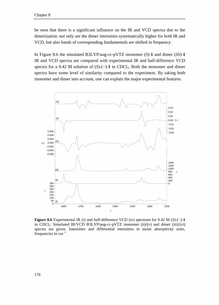
Chapter 8
176
be seen that there is a significant influence on the IR and VCD spectra due to the dimerization: not only are the dimer intensities systematically higher for both IR and VCD, but also bands of corresponding fundamentals are shifted in frequency. In Figure 8.6 the simulated B3LYP/aug-cc-pVTZ monomer (S)-1 and dimer (SS)-1 IR and VCD spectra are compared with experimental IR and half-difference VCD spectra for a 0.42 M solution of (S)-(−)-1 in CDCl3. Both the monomer and dimer spectra have some level of similarity compared to the experiment. By taking both monomer and dimer into account, one can explain the major experimental features.
1800 1700 1600 1500 1400 1300 12000
50100150200250300350
ε
Δ ε
ε
Δ ε
ν
(i)
0200400600800100012001400
(iii)
(ii)
-0.03
-0.02
-0.01
0.00
0.01
0.02
0.03
(v)
(vi)
-0.006-0.004-0.0020.0000.0020.0040.006
(iv)
Figure 8.6 Experimental IR (i) and half-difference VCD (iv) spectrum for 0.42 M (S)-(−)-1 in CDCl3. Simulated IR/VCD B3LYP/aug-cc-pVTZ monomer (ii)/(v) and dimer (iii)/(vi) spectra are given. Intensities and differential intensities in molar absorptivity units, frequencies in cm−1
Carboxylic acids – VCD perspective
References p.220 177
To interpret the experimental IR and VCD spectra in terms of the DFT results, however, the conformational populations need to be assessed for both monomer and dimer. The theoretical populations based on the free energy differences between monomer and dimer structures are often largely overestimated.25,51 Nonetheless, information on the fractions of monomer and dimer is embedded in the concentration dependence of the IR band intensities. Using a procedure similar to that described in Chen et al.,52 it was possible to extract this information by determining the equilibrium constant between monomer and cyclic dimer. The equilibrium for dimerization
M + M D is characterized by the dimerization constant [ ] [ ]2D MK = . This constant K can be
determined by analyzing the integrated absorbance in function of the analytical concentration of the dissolved species.52 In this approach, the experimental data are fitted to
( )
0
2 2
1 1 2
m mm m
c Kl AA lε ε
= + (8.2)
in which 0 2
mc A is plotted versus 1mA− . c0 refers to the analytical concentration of the
dissolved species 1, Am and εm are respectively the integrated absorbance and molar absorptivity of a distinct monomer band and l is the path length (0.02 cm). The model used in this study to approximate the monomer/dimer fractions is based on two individual equilibria between monomer and dimer, that is, an equilibrium between hydrogen bonded monomer (A/B) and the dimer and an equilibrium between the cis configured monomer (C, D, E and F) and dimer. Several approximations are used: First, the formation of trimers and tetramers and other solute-solute associations are not considered. Further, possible solvent-solute aggregation is not taken explicitly into account and the concentrations of the CHCl3/CDCl3 are not exact due to the volatile nature of this solvent. It has also come to our attention that the CHCl3 used in this study contains 0.5 to 1% EtOH for

Chapter 8
178
stabilization.‡ The mole fraction EtOH is too low, however, to have any influence on the dimerization equilibrium. Taking into account the aforementioned approximations and limitations of the model, the error on the determined populations is expected to be on the order of 10–15%. However, exact populations are not pursued in this study, but merely tentative values are intended that allow the assessment of experimental IR and VCD in terms of DFT results. The preferred region to extract population dependent data from the concentration series is the carbonyl stretch region, in which both the monomer and dimer bands are separated and do not coincide with other modes. The OH stretch region is less appropriate as there are many intense solvent bands present and also the CH stretch modes overlap with the dimer OH stretch modes. In Figure 8.7, the infrared absorbance spectra are given for the concentration series experiment in CHCl3 (same as Figure 8.4a but in absorbance units). As the solubility of 1 in CS2 is low, it was difficult to get solutions with accurate concentrations and consequently, the dimerization equilibrium constants for (R)-(+)-1 in CS2 could not be determined accurately. The integrated intensities for the monomer bands P1 and P2 and the dimer band P3, obtained by Lorentzian fitting, are given in Table 8.3 for the CHCl3 experiment. If 0 2
mc A is plotted versus -1mA (Figure 8.7), for the two equilibria
defined in our model, the dimerization constants can be determined with Equation (8.2) on the basis of the intercept and the slope of the linear fit. K1, being the equilibrium constant for the formation of cyclic dimer from monomer A and B, was determined to be 2.7 (ΔG1
0 = −0.6 kcal/mol). In the same way, for the equilibrium between the monomers with a cis configured carboxyl (C, D, E and F) and the dimer, K2 was determined to be 6.9 (ΔG2
0 = −1.2 kcal/mol). The predicted free energy difference between conformations A/B and C/D/E/F based on our proposed model is 0.6 kcal/mol. This value agrees reasonably well with the B3LYP/aug-cc-pVTZ free energy difference between conformations B and C, i.e., 0.76 kcal/mol (Table 8.1). ‡ Zhao et al.53 describe that the polypeptide gramicidin undergoes dimerization in solution. Gramicidin is reported to have a different VCD in CDCl3 compared to CHCl3 solutions (which contains 1% EtOH) in the amide I region. Their IR signatures are the same in this region.

Carboxylic acids – VCD perspective
References p.220 179
Table 8.3 Integrated absorbances of CO stretching bands from the monomer, 1mA and
2mA , and those of dimer, dA , for different initial concentrations (c0, in M) of (R)-(+)-1 in CHCl3.
c0 1mA 2mA dA
0.40 33 26 96 0.30 27 19 69 0.20 20 13 44 0.10 10 6 15 0.04 6 4 9 0.02 3 2 4 0.01 2 1 2
1850 1800 1750 1700 16500.0
0.2
0.4
0.6
0.8
1.0
1.2
1.4
1.6
1.8
2.0
2.2
2.4
2.6
2.8
3.0
0.0 0.1 0.2 0.3 0.4 0.5 0.6 0.70.00000.00050.00100.00150.00200.00250.00300.00350.00400.0045
0.0 0.2 0.4 0.6 0.8 0.0000.0010.0020.0030.0040.0050.0060.007
c0 /A2 m
2
1/Am2
1/Am1
ν
0.4M 0.3M 0.2M 0.1M 40mM 20mM 10mM
A
c0 /A2 m
1 P3
P2
P1
r2=0.99
r2=0.97
Figure 8.7 IR spectra of (R)-(+)-1 in CHCl3 for different concentrations varying between 0.4 M and 10 mM). The two subplots represent the linear plot based on Equation (8.2) for band P1 (top) and band P2 (bottom) – Correlation coefficients r2 are given. Intensities are in absorbance units, frequencies in cm−1. Defining df as the fraction of dimer,
1mf as the fraction of monomer A/B and 2mf as
the fraction monomer C/D/E/F; on can write the following expressions for the different fractions within our proposed model:
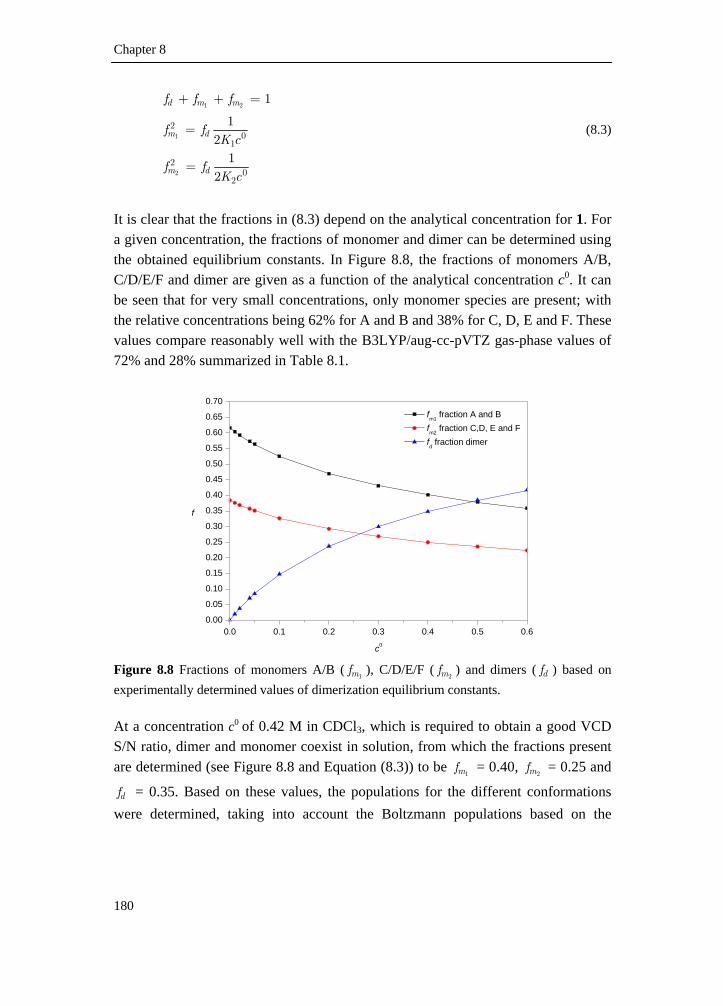
Chapter 8
180
1 2
1
2
20
1
20
2
1
12
12
d m m
m d
m d
f f f
f fK c
f fK c
+ + =
=
=
(8.3)
It is clear that the fractions in (8.3) depend on the analytical concentration for 1. For a given concentration, the fractions of monomer and dimer can be determined using the obtained equilibrium constants. In Figure 8.8, the fractions of monomers A/B, C/D/E/F and dimer are given as a function of the analytical concentration c0. It can be seen that for very small concentrations, only monomer species are present; with the relative concentrations being 62% for A and B and 38% for C, D, E and F. These values compare reasonably well with the B3LYP/aug-cc-pVTZ gas-phase values of 72% and 28% summarized in Table 8.1.
0.0 0.1 0.2 0.3 0.4 0.5 0.60.00
0.05
0.10
0.15
0.20
0.25
0.30
0.35
0.40
0.45
0.50
0.55
0.60
0.65
0.70 fm1 fraction A and B fm2 fraction C,D, E and F fd fraction dimer
f
c0
Figure 8.8 Fractions of monomers A/B (
1mf ), C/D/E/F (2mf ) and dimers ( df ) based on
experimentally determined values of dimerization equilibrium constants. At a concentration c0 of 0.42 M in CDCl3, which is required to obtain a good VCD S/N ratio, dimer and monomer coexist in solution, from which the fractions present are determined (see Figure 8.8 and Equation (8.3)) to be
1mf = 0.40, 2mf = 0.25 and
df = 0.35. Based on these values, the populations for the different conformations were determined, taking into account the Boltzmann populations based on the

Carboxylic acids – VCD perspective
References p.220 181
relative free energies of each subgroup of structures, that is monomer A/B (1mf ),
monomer C/D/E/F (2mf ) and dimer ( df ). In Table 8.4 the experimentally based
populations are given for B3LYP/aug-cc-pVTZ data. It has to be mentioned that the experimentally determined equilibrium fractions could be somewhat biased by solvent-solute interaction, which was not taken explicitly into account when modeling the conformations. Table 8.4 Experiment based populations (B3LYP/aug-cc-pVTZ) for monomer and dimer of 1 in CDCl3.*
% P % P % P % P A 23 FC 6 EC 4 ED 3 B 17 D 6 CC 3 FE 2 DC 8 F 6 FD 3 DD 2 C 8 E 6 FF 3 EE 1 *
1mf = 0.40, 2mf = 0.25 and df = 0.35
The simulated B3LYP/aug-cc-pVTZ and experimental IR and VCD spectra (experimental VCD spectra are half difference spectra) for three different concentrations (0.21, 0.25, and 0.42 M) are shown in Figure 8.9. The simulated spectra are averaged over all significant dimer and monomer conformations. The populations are calculated by determining the fractions of monomers and dimers for the three different concentrations using Equation (8.3) and taking into account the B3LYP/aug-cc-pVTZ Boltzmann populations. Here, the earlier discussed concentration dependence in the CO stretch region is visible, but a small effect is also seen in the 1300–1400 cm−1 area. For the VCD, a more pronounced concentration effect is observed. For higher concentrations more intense CO stretch dimer bands (fundamental 74 and 73) are observed, but the monomer VCD intensities for fundamentals 29A+B and 27/28 are reduced as are the monomer IR intensities of fundamental 34A+B and 30/29A+B. This obviously indicates that the dimer fraction increases at higher concentrations. The same effects can be observed in the simulated spectra (Figure 8.9 (ii) and (iv)), which indicates that our proposed model works.

Chapter 8
182
0
100
200
300
400
500
-0.008
-0.006
-0.004
-0.002
0.000
0.002
0.004
0.006
0.008
1800 1700 1600 1500 1400 1300 1200 11000
50
100
150
200
250
300
350
(i)
Δ ε
Δ ε
ε
29A+B30
34A+Bε
ν
(ii)
-0.020
-0.015
-0.010
-0.005
0.000
0.005
0.010
0.015
0.020 0.21 M 0.25 M 0.42 M
(iv)
74DC+CC
73DC/CC
74
29A+B
27/28
(iii)
Figure 8.9 Experimental spectra for (S)-(−)-1 in CDCl3 for three concentrations (0.21, 0.25, and 0.42 M) and B3LYP/aug-cc-pVTZ simulated IR/VCD spectra taking into account monomer and dimer of (S)-1 based on experimental populations for different concentrations (0.21 M, 0.25 M and 0.42 M). Intensities and differential intensities in (differential) molar absorptivity units, frequencies in cm−1. In Figure 8.10 (i) and (iii) the experimental IR and half difference VCD spectra for (S)-(−)-1 are given. The infrared region beneath 1000 cm−1 has a bad S/N ratio due to the high absorption of CDCl3 in that region. The long-wave cutoff from the optical filter and the CaF2 windows make that there is no reliable VCD signal observable below 1200 cm−1. Using a different setup with KBr windows and CS2 as solvent, the spectroscopic window is extended to 800 cm−1. Using CS2 as solvent, the fractions of monomer appear to be lower than those in CHCl3, but this effect is rather small on the IR and VCD spectrum, as can be seen in Figure S8.2 in

Carboxylic acids – VCD perspective
References p.220 183
Supplementary Material. Accordingly, the ‘CDCl3’ weighted spectra can be used without any problems for comparison with the experimental CS2 spectra. In Figure 8.10 (ii) and (iv) the simulated B3LYP/aug-cc-pVTZ spectra are shown, which are averaged over all the significant (S)-1 monomer and (SS)-1 dimer conformations using the experimental populations given in Table 8.4 (0.42 M). These simulated spectra can be compared to the experimental (S)-(−)-1 spectra. The B3LYP/aug-cc-pVTZ bands are labeled with their corresponding normal modes. Naturally, monomer and dimer bands overlap, which makes it difficult to assign the bands in much detail. However, where possible, in Figure 8.10 for monomer and dimer, the bands are assigned to the most contributing conformations (indicated by the conformational label). If the normal modes of different conformations have only a small frequency separation, the conformations are not explicitly mentioned in the labeling. The normal modes of the monomers for the 800–1850 cm−1 frequency interval run from 12 to 34, for the dimeric structures from 27 to 73. The monomeric labels are given in black, the dimeric in orange. In the carbonyl stretching region, a complex pattern can be observed in the IR and in the VCD (Figure 8.10). The most intense band in the IR can be attributed to the CO asymmetric stretch in the dimer (fundamental 74). The dimeric CO stretch modes (fundamentals 73 and 74) have lower vibrational frequencies than their monomeric counterpart (fundamental 34). This is due to the hydrogen bonding, which results in a cooperative lengthening of the C=O and OH bonds and a shortening of the C−O bond.3 Notwithstanding the fact that the calculated frequency splitting between the monomeric and dimeric CO stretch frequencies is somewhat overestimated, the IR/VCD for the CO stretching region shows a good agreement with the simulated spectra. Monomeric and dimeric bands can be observed and assigned to calculated bands. Bands 34 from conformations C, D, E and F (34C+D, 34F+E) are unresolved in the IR but can be recognized in the VCD. For the asymmetric CO stretch (mode 73), a negative VCD band is observed, mainly attributable to conformation DC and CC. The other dimer conformations are predicted to have a positive VCD for mode 73, but this cannot be observed in the experimental VCD.

Chapter 8
184
0100200300400500600700800900
1000110012001300
-0.03
-0.02
-0.01
0.00
0.01
0.02
0.03
1800 1600 1400 1200 1000 800
ε
Δ ε
Δ ε
19B+
F
25
ν
ε
(i)
38-35
39
17-15
44/4319/20
46/4
5
23/2
250
-47
19A60-56
29-25a+f
61/6
2
54/5
3
24
29A
+B3069/7
032
33
65
71/7
2
7434
34A
+B
68-6
631
0
50
100
150
200
250
300
350
400
450
(iii)
38/3
739
36/3
5
34/3
1
30/2
9
17
1615
14
13
27/2
812
A
44/4
319
/20
46/4
520
A
23/2
250
-47
21
19A
+B+F
1842
/41
4060-5
629
-26
61/6
2
56/5
5/54
53FC
+FD
+EC
+ED
54D
C+C
C
24
25/2
6C+D
29A
+B30
70-6
6
73 32/3
1
33
65
71/7
2
74
34F+
E34
C+D
(ii)
34A+
B
x4
x4
-0.015
-0.010
-0.005
0.000
0.005
0.010
0.015
12A
1227
28
36EC+CC-32/31FF
18B
53FC/FD/EC/ED
34A
+B
74
73D
C+C
C
74D
C+C
C34
F/E
34C
+D
56D
C/5
5/54
FF/5
3FF
57/5
6 25
27C
+D/2
6B+E29
F+E
/28F
+E
68-6
631
64/6
3
28/2
7
62/61 54CC/DC
25A
+F/2
6C+D
29A+B
30/2
9C+D
69/7
032
33
6571/7
247-50
50/4
9
20F/C
23E/22A+C
23A+
D+F
44/4
3
19/2
0
46/45
23B
24
38-3517F/16D
19A
19B
39
27
16-14
12A
47-5
050
/49
18E
41C
C/4
2
38D
C+F
D+E
D
35FD
+FF/
36
37/3
8
14
17F/
16D
19A
19B
18B
19
20F/
C20
A21
D
23E
/22A
+C23
A+D
+F
56D
C/5
5/54
FF/5
3FF
57/5
661
FF/6
2FF/
60-5
8
25
27C
+D/2
6B+E
26F/
28D
29F+
E/2
8F+E68-6
631
73
7474
FF
(iv)
39
44/4
3
36EC
+CC
-32/
31FF
32/3
1 30/2
9
17
1615
13
43FF
+FD
+FC
/44F
F20
46/4
5
21A
23B
21
42FF
+FD
/41
40
64/6
3
28/2
762
/61
53FC
+FD
+EC
+ED
54C
C+D
C
24
25A+
F/26
C+D
29A
+B30
/29C
+D
69/7
0
73D
C+C
C 3233
6571/7
2
74D
C+C
C
34F/
E34
C+D
34A
+B
Figure 8.10 IR (i) and half-difference VCD (iii) spectrum for 0.42 M (S)-(−)-1 in CDCl3 (intensities are multiplied with factor four). For the <1200 cm−1 region the CS2 spectrum is given (~0.11 M). B3LYP/aug-cc-pVTZ simulated IR (ii) and VCD (iv) spectra taking into account monomer and dimer of (S)-1 based on experimental populations. Intensities and differential intensities are in molar absorptivity units, frequencies in cm−1. In the spectral region between 1500 and 850 cm−1, a complex spectrum is observed with several unresolved and broad bands. The VCD spectrum in this region has some distinct features, which allows, in combination with the IR spectrum, the assignment of experimental bands. Monomeric fundamentals 29 to 25 coinciding with dimeric fundamentals 60 to 56 are not resolved in the IR, which is in agreement with predictions. Some IR bands can be exclusively assigned to dimer structure vibrations, i.e., bands 74, 73, 65, 54DC+CC, 53FC+FD+EC+ED, 46/45, 42/41, 40,

Carboxylic acids – VCD perspective
References p.220 185
and for the VCD, bands 74DC+CC, 74, 74F, 73DC+CC, 73, 65, 54CC+DC, 53FC+FD+EC+ED, 42FF+FD/41, 40, 39. Exclusive monomeric bands in the IR are 34A+B, 34, 30, 19B+F and for the VCD 34A+B, 34C+D, 34 F+E, 27/28, 24, 19A, 19B. The other bands must be assigned to coinciding dimer and monomer fundamentals. If small differences are neglected, it can be concluded that almost all experimental IR and VCD bands can be assigned with success to the harmonic fundamentals. Some larger bands cannot be observed in the experimental spectra, i.e., VCD band 73 (discussed earlier), VCD band 21A (COH bend), bands 42/41/40 (mainly COH out of plane bend) and VCD band 13/30/29 (CH2 rocking). As these differences are found for both the 6-31++G** and the aug-cc-pVTZ basis set, it is highly unlikely that this is the effect of the use of an incomplete basis set. To investigate the effect of the density functional, six additional functionals (B1LYP, B3P86, B3PW91, B98, MPW1PW91, PBE1PBE) were used to simulate IR and VCD spectra for 1 using the 6-31++G** basis set. These resulting spectra are given in Figures S8.3 and S8.4 (Supplementary Material). The overall agreement between simulated and experimental spectra is best for the B1LYP and B3LYP functionals. It can also be seen that all the functionals fail to correctly predict the rotational strength of fundamental 73 (selected conformations, see above), fundamental 21 for conformation A, and combined fundamentals 13, 30 and 29. For the B3PW91 and B3P86 functionals, the vibrational frequencies for fundamentals 42, 41 and 40 are shifted somewhat to higher wavenumbers and show a better resemblance with the experimental spectrum for this part of the spectrum compared to the B3LYP functional. However, fundamentals 40, 41 and 42 correspond to COH out of plane bending modes. In a recent study,54 Antony et al. found that the harmonic COH out-of-plane bending frequency for dimeric benzoic acid is gravely overestimated by ~50 cm−1 due to the anharmonic character of this vibrational mode. If this argument is pursued, it would mean that the predicted frequencies for fundamental 40–42 are overestimated and these would be shifted to lower wavenumbers in the experimental spectra. If these corresponding bands are lowered by 50 cm−1, these would coincide with intense profiles in both IR and VCD bands. This would also explain the relative intensity of the IR band 17–15/38–35. Taking into account the approximations that are used to determine the monomer and dimer populations to simulate their IR and VCD spectra, it would be of no use to perform a quantitative comparison of simulated and experimental spectra which is sometimes performed,13,50 for smaller molecules. In this study the situation is even

Chapter 8
186
more difficult because not only bands of different conformations, belonging to one species coincide, but also bands from dimer conformations can overlap with bands of the monomer conformations. As a result, no quantitative comparison is performed. However, the assignment of the bands to fundamentals by comparison of the experimental and theoretical spectra was still possible and the resulting agreement in both spectra and trends establishes that for this specific molecule, both monomeric and dimeric species are present and that these can be modeled to simulate spectra. 8.2.6 Conclusion
It this study it is shown that for a carboxylic acid 1 in CS2 and CDCl3, considerable fractions of monomer exist next to cyclic dimers, due to the stabilizing effect of an intramolecular hydrogen bonding for two monomer conformations. The equilibrium between the monomer and the cyclic dimer was evaluated using a concentration variation study in CHCl3. The proposed model that describes the equilibrium between intramolecular stabilized monomer and cyclic dimer and nonintramolecular bonded dimer and cyclic dimer predicts monomer equilibrium concentrations that are 60% higher for the stabilized monomer form. The amount of cyclic dimer was found to be dependent on the initial amount of 1 present in CHCl3. Taking into account the equilibrium between monomer and dimer, IR and VCD spectra were simulated for (S)-1 on the basis of the approximate experimentally determined fractions and B3LYP/aug-cc-pVTZ Boltzmann populations of dimeric and monomeric conformations. Spectra were simulated at the B3LYP/aug-cc-pVTZ level and were compared with experimental spectra for (S)-(−)-1 in CDCl3 and CS2. A good agreement was obtained which suggests that the proposed model of dimer/monomer equilibrium is valid within the scope of our article. 8.2.7 Supplementary material index
For this paragraph Supplementary Material is provided. It can be downloaded from http://www.quantum.UGent.be/tksup.pdf Table S8.1 B3LYP/6-31++G** conformational description monomer 1 Table S8.2 B3LYP/ cc-pVTZ conformational description monomer 1 Table S8.3 B3LYP/ 6-31++G** conformational description dimer 1

Carboxylic acids – VCD perspective
References p.220 187
Table S8.4 B3LYP/aug-cc-pVTZ monomer normal modes Table S8.5 B3LYP/aug-cc-pVTZ dimer normal modes Figure S8.1 The OH and CO stretching regions for solutions of (R)-(+)-1 in CS2
Figure S8.2 CDCl3 and CS2 simulated and experimental spectra Figure S8.3 Simulated IR DFT/6-31++G** spectra for different functionals Figure S8.4 Simulated VCD DFT/6-31++G** spectra for different functionals

Chapter 8
188
8.3 Elucidation of the absolute configuration of
tetrahydrofuran-3-carboxylic acid
8.3.1 Introduction
In the previous paragraph the intermolecular association of tetrahydrofuran-2-carboxylic acid was described using unpolarized IR and VCD methods. All plausible monomer and cyclic dimer conformations of the carboxylic acid were accounted for in the simulation of theoretical IR and VCD spectra. In this paragraph, the absolute configuration of tetrahydrofuran-3-carboxylic acid, a position isomer of the previous compound, is elucidated taking into account the formation of cyclic dimers. Using DFT, the monomers and cyclic dimers were modeled and the corresponding IR and VCD spectra could be simulated. These theoretical spectra, in turn, could be compared to experimental data, which were provided by Johnson & Johnson Pharmaceutical Research and Development (JNJPRD). This analysis is part of an agreement between Ghent University and JNJPRD in which AC determinations are performed on drugs discovery compounds (for more information see the Appendix). VCD has partially replaced XRD AC determinations at JNJPRD, as VCD has obvious advantages compared to other methods 8.3.2 Experimental
The enantiopure samples, i.e., (+)-2 ( α24
D = +21.44 (EtOH)) and (−)-2 ( α20D = −21.91
(EtOH)) were obtained by separation of the racemic mixture (Aldrich) using chiral column chromatography.55 The experimental IR and VCD spectra for both enantiomers were provided by JNPRD. VCD and IR data within the 1000–1500 cm−1 frequency interval were available. Details concerning experimental conditions are not known, but the sample concentrations provide a reliable VCD as the majority of IR bands reside within 0.2–0.8 absorbance unit interval. Solutions were prepared with CD2Cl2. Further, the half-difference VCD spectrum is reported, calculated as ( )/2A A+ −Δ − Δ . Additional, unpolarized IR data were provided for the CO and OH stretch region.

Carboxylic acids – VCD perspective
References p.220 189
8.3.3 Computational methods
The conformational search strategy and computational methods are the same as those used in §8.2. The B3LYP functional was used in combination with the 6-31G* and 6-31++G** basis set for respectively the (R)-2 monomer and (RR)-2 dimer. Previously (§8.2) it was shown that the B3LYP/6-31++G** level is sufficient to describe carboxylic acid dimer geometries in the context of IR and VCD comparison. A scaling factor of 0.967 is used to correct for the harmonic approximation.16 8.3.4 Results and discussion
8.3.4.1 Conformational description
In Table 8.5, the conformational description is given for the (R)-2 monomer. The same descriptors are used as for 1 in §8.2, i.e., puckering coordinates for the five membered rings and the dihedral angles as defined in Figure 8.11. Based on the configuration of the carboxylic acid moiety (τ2), the conformations can be categorized in two classes, that is, the hydroxyl group can be cis or trans relative to the carbonyl group. It can be observed, in Table 8.5, that the trans conformers have a higher energy compared to the cis isomers. For one trans conformations, i.e., conformer F, hydrogen bonding with the THF oxygen is observed, which has a stabilizing effect. Compared to 1, this stabilizing effect is relatively small and the cis conformations are found to be more stable. In Figure 8.12 the 4 cis minima (A, B, C and D) and also the intramolecular hydrogen bonded minimum F are depicted.
O
O
O
H
1
2
34
5
7
6
8
9
τ1
τ2
Figure 8.11 Depiction of 2 and definition of dihedral angles τ1 and τ2

Chapter 8
190
For the (R,R)-tetrahydrofuran-3-carboxylic acid dimer a total of 15 conformations were found which are described in Table 8.6. If Table 8.5 and Table 8.6 are closely compared, it can be seen that the monomer geometries are building blocks that can be used for the construction of cyclic dimer structures, with only one exception, that is conformation B’C. This is the global minimum dimer structure which is constructed from the C and B’ monomer. The geometry of the monomeric B’ differs from B in the dihedral angle τ1. Clearly, the dimeric dihedral angles T1 and T1’ (and also the THF ring geometries) for all dimer structures deviate slightly from their corresponding monomeric dihedral angles τ1, but in case of dimer B’C the difference is rather large (Δτ1 = 27°). The monomeric B’ geometry, however, is not found as an optimum. In Figure 8.12, a model representation for the B’C dimer is given.
O
O
O H
O
O
OHT1
T'1
Figure 8.13 Depiction of cyclic dimer 2 and definition of dihedral angles Τ1 and Τ’1 Table 8.5 B3LYP/6-31G* label, pseudo-rotational coordinates (q in Å and φ in degrees), key dihedral angles (τ1 and τ2 in degrees), relative free energies (ΔG0 in kcal/mol) and Boltzmann populations (% P, 298.15 K) for the unique monomer minima of 2.
q φ τ1 τ2 ΔG0 % P A 0.38 50 158 −1 0.00 47.7 B 0.38 174 76 0 0.31 28.5 C 0.37 8 71 1 0.65 16.1 D 0.39 156 −61 0 1.50 3.8 E 0.38 38 −59 0 1.51 3.8 F 0.42 329 −42 −178 3.49 0.1 G 0.39 151 107 −179 5.49 0.0 H 0.38 193 171 180 6.66 0.0 I 0.37 305 69 −179 6.83 0.0 J 0.38 137 −57 −179 6.90 0.0 K 0.37 11 72 −178 6.91 0.0 L 0.38 27 −175 −179 6.94 0.0 M 0.37 189 −64 −179 8.24 0.0
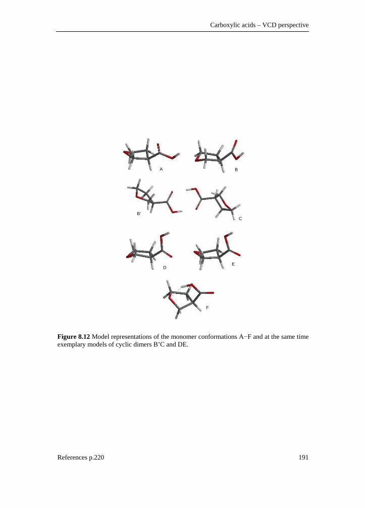
Carboxylic acids – VCD perspective
References p.220 191
A B
B'C
DE
F
Figure 8.12 Model representations of the monomer conformations A−F and at the same time exemplary models of cyclic dimers B’C and DE.

Chapter 8
192
Table 8.6 B3LYP/6-31++G** label, symmetry, pseudo-rotational coordinates (q in Å and φ in degrees), key dihedral angles (Τ in degrees), relative enthalpies (ΔH0 in kcal/mol), relative free energies (ΔG0 in kcal/mol) and Boltzmann populations (% P, 298.15 K) for the unique dimer minima of 2.
Label q1 φ1 Τ1 q2 φ2 Τ2 ΔH0 ΔG0 % P B'C C1 0.38 167 103 0.37 18 76 0.39 0.00 74.5 DB C1 0.38 180 −70 0.38 179 82 0.54 1.49 6.1 EB C1 0.38 45 −60 0.37 176 78 0.87 1.64 4.6 BB C2 0.38 179 79 0.37 179 80 0.00 1.83 3.4 DA C1 0.38 178 −67 0.38 49 149 1.03 2.15 2.0 AC C1 0.38 42 156 0.37 14 75 0.72 2.19 1.8 BA C1 0.37 180 78 0.38 41 157 0.47 2.20 1.8 CD C1 0.37 17 77 0.38 176 −69 0.80 2.43 1.2 EA C1 0.38 46 −62 0.38 47 152 1.38 2.44 1.2 ED C1 0.38 43 −54 0.38 177 −66 1.39 2.65 0.9 EC C1 0.38 46 −65 0.37 11 71 1.10 2.70 0.8 AA C2 0.38 39 162 0.38 39 162 0.95 2.89 0.6 DD C2 0.38 178 −66 0.38 183 −67 1.09 2.95 0.5 CC C2 0.37 17 76 0.37 17 76 0.51 3.01 0.5 EE C2 0.38 43 −59 0.38 43 −63 1.73 3.59 0.2
8.3.4.2 IR and VCD spectra
In Figure 8.14 (i) and (iv) the experimental IR and VCD for (+)-2 are given. The VCD spectrum is actually the half difference spectrum. The simulated spectra for (R)-2 can also be found in Figure 8.14; the monomer spectra in subplots (ii) and (v), the dimer spectra in subplots (iii) and (vi). Due to the unknown concentrations the absorbance spectra could not be converted into molar absorptivity units. However, ignoring the differences in intensity units, a good proportional agreement can be noticed between the simulated dimer and experiment. Also, applying the Lambert-Beer law and Equations (4.2) and (4.3) to creating molar absorptivity spectra, will not change the observed proportional agreement. This approach, albeit pragmatic, allows a reliable assignment of experimental bands based on harmonic fundamentals.

Carboxylic acids – VCD perspective
References p.220 193
The influence from monomer and dimer conformations on the IR and VCD for this compound is likely to be different than for the 2 isomer. Based on the conformational search, the former compound is not expected to form stabilizing intramolecular hydrogen bonds, ergo compared to 1 the dimer-monomer equilibrium is expected to be shifted more to the dimer.
1800 1600 1400 12000.0
0.2
0.4
0.6
0.8
1.0
1.2
1.4
(ib)
ε
Δ ε
Α
Δ Α
ν
(ia)
x0.2
0
400
800
1200
(iii)
(ii)
-0.03-0.02-0.010.00
0.010.020.03
(v)
(vi)
-0.15
-0.10
-0.05
0.00
0.05(iv)
Figure 8.14 Experimental IR (ia absorbance scaled with factor 0.2 and ib) and half-difference VCD (iv) spectrum for (+)-2 in CD2Cl2. Simulated IR/VCD B3LYP/6-31++G** monomer (ii)/(v) and dimer (iii)/(vi) spectra for (R)-2. Experimental intensities and differential intensities in absorbance units. Theoretical intensities and differential intensities in molar absorptivity units, frequencies in cm−1

Chapter 8
194
3800 3600 3400 3200 3000 2800 2600
0.0
0.1
0.2
0.3
ν
Α
(i)
0
2000
4000
6000
8000
10000
(ii)
ε
x50
Figure 8.15 (i) OH stretch region IR spectrum of 2 in CD2Cl2 and (ii) theoretical 6-31G* (intensities scaled x50) monomer (in blue) and 6-31++G** dimer spectrum. In Figure 8.14(i) and 8.15(i) the OH and CO stretch spectra are given for a CD2Cl2 2 solution. Based on the CO stretch region, in Figure 8.14(ia), it is difficult to assess if there is monomer present in solution. Monomer signatures are seen but these are relatively weak. In the OH stretch region, it can clearly be seen that fractions of monomer are present, with two relatively weak bands near 3700 cm−1 and 3500 cm−1. However, to draw quantitative conclusions for the equilibrium between monomer and dimer, a concentration study has to be performed, in which multiple solutions with known concentrations should be measured. These kind of data were not provided, and also, the assessment of the equilibrium is not within the scope of this study, which is primarily to establish the absolute configuration of the provided samples. It can be observed in Figure 8.14, that the predicted monomer IR and VCD intensities are also relatively small. If the monomer structures had any significant populations, which is doubtable based on the previous observations, it can be said that the monomer contribution would be insignificant due to the small predicted intensities and their small influence on the total Boltzmann weighted spectrum. The VCD spectra are therefore simulated only taking into account cyclic dimer structures, discarding the presumable small fraction of monomer.

Carboxylic acids – VCD perspective
References p.220 195
8.3.4.3 Fundamental assignment
In Figure 8.16 and 8.17 the experimental bands are assigned based on the B3LYP/6-31++G** dimer fundamentals. The experimental bands can be assigned based on the agreement between simulated and experimental IR and VCD. Virtually all bands can be explained by considering the two lowest energy minima for the dimers, i.e., minima B’C and DB, as they constitute more than 80% of the total population over all the minima listed in Table 8.6. For both conformations, the transition frequency and dipole/rotational strengths can be found in Table 8.7 for fundamentals 41–72. Based on these data and within the applied approximation, a relatively good assignment can be done. In Figure 8.16 the experimental IR spectrum is given concurrently with the simulated dimer spectrum. The labels indicate the assigned fundamental, i.e., label a represents conformer B’C and b conformer DB. For the VCD data, the same can be seen in Figure 8.17. Two bands can be assigned to a unique conformation, i.e., bands 55a and 44b. Band 55a is an example of how an unresolved IR band can be identified using the VCD spectrum. In Figure 8.16 it can be seen that all IR bands have a good proportional agreement, except for band 42, which is predicted to be relatively weak. Fundamentals 54–51 are predicted to have a small frequency separation, giving rise to one band. Experimentally these appear as a broad band with two shoulders corresponding to fundamental 52 and 51/50. One band in the IR, near 1150 cm−1, could possibly be assigned as monomeric, as is was not possible to assign this to any dimer structure fundamental. In the VCD spectrum, the very small combined rotational strengths for fundamentals 61/60/59a are underestimated compared to the experiment, but have the same sign. Fundamental 47 could not be assigned and is possibly unresolved in agreement with its small predicted intensity. Fundamentals 44b and 43 are predicted to have a small frequency separation, but are experimentally found as 2 different bands.

Chapter 8
196
Table 8.7 B3LYP/6-31++G** vibrational frequencies (ν, in cm−1), dipole strengths (D, in 10−40 esu2cm2) and rotational strengths (R, in 10−44 esu2cm2) for two most significant (R,R)-dimer conformations, i.e., B’C and DB.
B’C DB ν D R ν D R 41 1029 94 27 1018 53 29 42 1051 173 67 1035 103 4 43 1063 203 −79 1059 153 −100 44 1080 194 66 1066 127 −86 45 1085 72 −30 1086 236 208 46 1092 139 88 1087 129 −15 47 1170 4 −5 1176 19 29 48 1183 23 −15 1177 34 −56 49 1184 51 36 1199 38 2 50 1199 6 −7 1200 5 −14 51 1221 13 −29 1224 93 32 52 1228 688 82 1229 440 −43 53 1230 43 −41 1230 84 5 54 1235 237 16 1258 19 34 55 1239 127 −40 1265 18 −19 56 1268 34 41 1274 159 47 57 1274 44 27 1280 7 11 58 1278 208 7 1291 113 32 59 1313 22 −1 1299 409 −15 60 1317 12 −5 1317 3 5 61 1335 307 −12 1320 7 −12 62 1340 67 22 1334 236 −2 63 1351 35 −12 1354 8 2 64 1352 66 −9 1355 76 −6 65 1418 449 22 1411 314 −3 66 1442 20 43 1437 48 61 67 1450 30 −56 1446 20 −18 68 1452 21 −38 1449 20 −91 69 1462 3 −4 1460 2 −3 70 1464 4 −2 1462 1 1 71 1477 2 0 1477 15 9 72 1478 12 5 1477 4 2
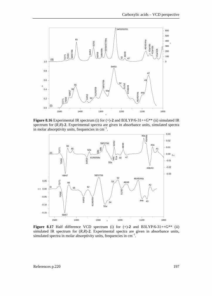
Carboxylic acids – VCD perspective
References p.220 197
1500 1400 1300 1200 1100 10000.0
0.2
0.4
0.6
0.8
1.0
68/6
7
ν
Α
(i)
6564
/63
6261
/60/
59 58/5
7/56
55a
54/53
52
51/5
047
/48/
49
46/4
5/44
a 44b
43
42
72/7
170
/69
66
68/6
7/66
65
64/6
362
/61
60/5
9
55/5
6/57
/58a
54/53/52/51
5048
/49
47
46/4
5/44
a
43a/
44b
42a/
43b
41a/
42b
72/7
170
/69
0
100
200
300
400
500
600
58b/
59b
ε
(ii)
Figure 8.16 Experimental IR spectrum (i) for (+)-2 and B3LYP/6-31++G** (ii) simulated IR spectrum for (R,R)-2. Experimental spectra are given in absorbance units, simulated spectra in molar absorptivity units, frequencies in cm−1.
1500 1400 1300 1200 1100 1000
-0.15
-0.10
-0.05
0.00
0.05
ν
Δ Α(i) 65
64/6
3
62
61/6
0/59
58/57/56
55a
54
5352
51/5
0
48/4946/45/44a
44b 43
42
-0.03
-0.02
-0.01
0.00
0.01
0.02
0.03
4145
/44a
50
58b
59b
Δ ε(ii)
72/7
170
/69
68/67
66
65
64/6
3
62a
61/60/59a
58/57/56
55a
54a
53/5
251
a
48/4
9
47
46a
44b/43
42a
72/7
170
/69
68/67
66
Figure 8.17 Half difference VCD spectrum (i) for (+)-2 and B3LYP/6-31++G** (ii) simulated IR spectrum for (R,R)-2. Experimental spectra are given in absorbance units, simulated spectra in molar absorptivity units, frequencies in cm−1.
Chapter 8
198
8.3.4.4 Absolute configuration assignment
The identification of the experimental bands is the first step in the process of the determination of the absolute configuration. If a good agreement is seen between vibrational frequencies and IR and VCD intensities, conclusions can be drawn about the three dimensional structure of the studied compound. However, in general, experimental dipole and rotational strengths should be derived from the experimental molar absorptivity spectra by Lorentzian fitting (see Chapter 4). As these molar absorptivity spectra are not available, it is not possible to determine the experimental dipole and rotational strengths and to correlate them with theoretical values. But, as previously reported for other compounds, it is still possible to perform a reliable assignment without this correlation, as the experimental bands are all thoroughly assigned. Experimental spectra of to (+)-2 in CD2Cl2 were compared to simulated spectra for the R configured cyclic dimer of 2. Based on the proportional agreement between the simulated and experimental IR and VCD, and the agreement of the VCD intensity signs it can be concluded that (+)-2 can be assigned as the R configuration. 8.3.5 Conclusion
For the compound under study, i.e., tetrahydrofuran-3-carboxylic acid, monomer IR and VCD spectra do not reproduce the experimental spectra. This is believed to be due to dimer formations for carboxylic acids in solution. Based on the conformational analysis it could be concluded that cyclic dimers are most significant, compared to other associations. Experimental spectra indicated that mainly dimers are present in solutions. This, combined with the low IR and VCD activity of the monomer, allowed that theoretical spectra could be simulated using B3LYP/6-31++G** cyclic dimers geometries. Based on these spectra, the experimental IR and VCD bands could be assigned using the two lowest energy cyclic dimer conformers. Experimental spectra corresponding to (+)-2 were presented together with the simulated spectra for the R configuration. A qualitative agreement was observed for IR spectra and VCD spectra. For virtually all bands, the VCD was predicted with the correct sign. Based on this agreement, it can be concluded that the sample with positive optical rotation agrees with (R)-2. Further conclusions on solvent-solute interaction and dimer-monomer equilibrium can not be drawn from this study, due to the lack of experimental data.

Carboxylic acids – VCD perspective
References p.220 199
8.4 A DFT conformational analysis and VCD study on methyl-
tetrahydrofuran-2-carboxylate
8.4.1 Scope and significance
In this last paragraph, a DFT study that was performed on methyl-tetrahydrofuran-2-carboxylate is presented. This compound is the corresponding methyl-ester of the carboxylic acid studied in §8.2. In the literature it was already established that conversion into the corresponding methyl-ester is a good method to study carboxylic acids with IR and VCD methods, without having to deal with the intermolecular aggregation.5 This is confirmed in this work. To extend the scope of this study, the potential energy surface and the spectra are thoroughly investigated using different hybrid functionals. Also, a new and promising similarity measure based on neighborhood similarity is introduced, which will be the ansatz for Chapter 9. 8.4.2 Introduction
An interesting approach for the synthesis of tetrahydrofuran-2-carboxylic acid is the enantioselective hydrolysis of its esters.6 (R)-tetrahydrofuran-2-carboxylic acid is a chiral building block for faropenem7, a clinically effective non-natural β-lactam antibiotic.8 In this paper, a study is performed on the methyl-ester of tetrahydrofuran-2-carboxylic acid using unpolarized infrared (IR) and vibrational circular dichroism (VCD) spectroscopy and density functional theory (DFT). VCD spectroscopy has become a powerful method to study the absolute configuration and the conformational properties of chiral molecules in solutions. Vibrational CD is the differential vibrational absorption between left and right circularly polarized IR radiation by a chiral species.56 In combination with quantum chemical calculations, experimental VCD spectra can be simulated which allows the interpretation of the experimental VCD. For a specific vibrational transition, Kuppens, T.; Vandyck, K.; Van der Eycken, J.; Herrebout, W.; van der Veken, B. J.; Bultinck, P. Spectrochim. Acta A 2006, In Press
Chapter 8
200
enantiomers have identical IR intensities. Their VCD intensities, however, are opposite in sign. Consequently, agreement between a simulated and experimental VCD spectrum should imply that the enantiomerically pure compound measured, has the same absolute configuration as the modeled compound. Evidently, this agreement depends on the reliability of the prediction. The most applied theoretical framework for the prediction of VCD intensities, consists in using DFT with the B3LYP hybrid functional10-12,35, combined with the application of the 6-31G* basis set. This combination has been used in numerous studies and gives satisfactory results, allowing the interpretation of the experimental VCD spectra of chiral molecules in solution.50,57,58 The absolute configuration of methyl-tetrahydrofuran-2-carboxylate, 3, is known from the synthesis, i.e., based on the absolute configuration of the corresponding carboxylic acid28,59 (+)-3 has the S configuration. The spectra measured for (+)-3 should therefore show a high degree of similarity towards the spectra simulated for (S)-3. The a priori knowledge of the AC allows to set up a study, in which the performance of the hybrid density functionals are screened for their applicability in the VCD methodology21,60 for the compound under study, applying the 6-31G* and cc-pVTZ basis sets. For each functional, IR and VCD spectra are simulated and compared in detail with the experiment, assigning experimental bands based on the harmonic fundamentals. Also, a similarity measure is introduced which allows the comparison of experimental and theoretical spectra, to establish the usefulness of the different hybrid functionals. 8.4.3 Methods
8.4.3.1 Preparation of (+)-(S)-methyl-tetrahydrofuran-2-carboxylate
(+)-(S)-methyl-tetrahydrofuran-2-carboxylate was made by esterification of (−)-(S)-tetrahydrofuran-2-carboxilic acid using diazomethane (98 % ee).59 This method proved superior over the use of commercial (CH3)3SiCHN2 since it resulted in an easier purification of the product.

Carboxylic acids – VCD perspective
References p.220 201
8.4.3.2 Spectroscopy
IR and VCD spectra are measured using respectively a Bruker Vector 22 and an IFS 66v/S FTIR spectrometer coupled to a PMA37 module.29 A demountable cell with CaF2 windows and a 105 µm Teflon spacer are employed. The unpolarized IR absorbance spectra are recorded at a resolution of 4 cm−1, the VCD spectra at a resolution of 6 cm−1. To improve the VCD S/N ratio a long wave-pass filter with an 1830 cm−1 cutoff is used. The collection time for the VCD spectrum is 90 minutes. (+)-3 is dissolved in CD2Cl2 at a concentration of 0.42 M and 0.68 M. The sample with high concentration was used to obtain good VCD spectra for the 1400–1500 cm−1 range. These spectra are provided in Figure 8.18.
1800 1700 1600 1500 1400 1300 1200 11000
50
100
150
200
250
300
(iib)
(iia)
ν
(i)
-0.010
-0.005
0.000
0.005
0.010
0.015
ε
Δ ε
Figure 8.18 Experimental IR (i) and VCD for 0.42 M (iia) (S)-(+)-3 solution in CD2Cl2. For the region 1400–1500 cm−1 the VCD (iib) is given for the 0.68 M solution due to the weak VCD in that area.

Chapter 8
202
To compensate for machine and cell artifacts, the VCD of the solvent was used as baseline, and was measured in the same conditions as the sample. In the past this has been proven to be a good approximation.17,61 8.4.3.3 Computation
Geometry optimizations and the calculation of the dipole strengths (D) and rotational strengths (R) are performed using Gaussian03 revision B532 using the tight optimization criterion. DFT calculations with the 6-31G* and cc-pVTZ basis set were performed using a set of 9 hybrid functionals, i.e., B1LYP, B3LYP, B3P86, B3PW91, B98, BHandH, BHandHLYP, MPW1PW91 and PBE1PBE.38 The conformational analysis is described further. For all the allocated DFT minima, for each functional using the cc-pVTZ62,63 basis set, the Hessian matrices, atomic polar tensors (APT) and atomic axial tensors (AAT) are calculated using gauge-including/invariant atomic orbitals (GIAOs)39,40, allowing the calculation of the dipole and rotational strengths. The enthalpy and Gibbs energy are calculated under the usual assumptions using standard statistical thermodynamical expressions.41 An appropriate scaling factor is used to correct for the harmonic approximation.64,65 All calculations were performed on the Ghent Quantum Cluster. 8.4.4 Results and discussion
Because VCD is very sensitive to conformational changes, the conformational description of the compound studied is very important.66,67 As a consequence, to ensure that all possible conformations with significant contributions can be located, a conformational search has to be performed with the greatest care. For this compound, first a preliminary MM343 and MM468 stochastic search with subsequent B3LYP/6-31G* optimization was performed, which indicated that two different ring conformations are possible for 3. To describe these ring conformations, Cremer-Pople pseudo rotational coordinates are used; the puckering amplitude q describes the degree of ring puckering and the pseudo-rotational phase angle φ describes the mode of ring puckering.46,47,69 Also, methyl-ester conformations with a trans configuration, i.e., τ2 = 180° (O7C6O8C9 in Figure 8.19) showed to be higher in energy compared to the cis configured minima (ΔH0
min(B3LYP/6-31G*) > 7 kcal/mol).

Carboxylic acids – VCD perspective
References p.220 203
O
O
OCH3
1
2
34
5 6
7
89
τ1 τ2
Figure 8.19 Depiction of 3 and definition of dihedral angles τ1 (O1C2C6O8) and τ2 (O7C6O8C9) Subsequently, a systematic B3LYP/6-31G* search was applied for cis (τ2 = 0°) configured (S)-3 in which τ1 (O1C2C6O8) is varied in steps of 5° for two different sets of puckering coordinates, i.e., q = 0.36 Å/φ = 120° and q = 0.38 Å/φ = 230°. A total of 144 starting geometries were optimized using a tight optimization criterion yielding 4 minima. The same systematic search was performed using a series of alternative hybrid functionals, i.e., B1LYP, B3P86, B3PW91, B98, BHandH, BHandHLYP, MPW1PW91 and PBE1PBE. However, the energy order and the number of located minima were found to depend on the functional used (See Table S8.6 in Supplementary Material). In order to gain some transparency on the conformational behavior of the compound under study, a B3LYP/6-31G* constrained potential energy surface scan was performed, developing τ1 in steps of 1°, for both ring conformations. The constrained energy profile can be found in Figure 8.20 in which 6 possible minima can be distinguished, which are labeled T, U, V, W, X and Y. As can be seen, in Figure 8.20, the constrained energy profiles are not well defined for the 90°<τ1<160° region, probably due to the steric hindrance between the carbonyl moiety and the THF ring.

Chapter 8
204
50
100
150
100150200250
0 100 200 300
0.0
0.5
1.0
1.5
2.0
2.5
3.0
3.5
4.0
(i)
Y UV
X
T
W
(ii)
100 110 120 130 140 150 160
0.160.180.200.220.240.260.280.30
ϕ
ϕ
τ 1
Δ E
Figure 8.20 B3LYP/6-31G* constrained energy profile for two different ring conformations with initial geometry descriptors q = 0.36 Å/φ = 115° (i) and q = 0.38 Å/φ = 230° (ii). The dihedral angle coordinate τ1 is kept fixed during the optimization (scanned in steps of 1°). Relative SCF energies are given in kcal/mol. The puckering angle (φ, in degrees) as a function of the dihedral angle coordinate τ1 is given above each energy profile. The same scans were performed again for the 50° < τ1 < 190° region, using a tight optimization criterion (red). The subplot in (ii) is a detailed energy plot of the 90° < τ1 < 160° region The geometries equivalent to the points labeled T, U, V, W, X and Y on the constrained energy profiles in Figure 8.20 are taken as starting geometries for the tight optimization, employing a cc-pVTZ basis set and a set of 9 different functionals. In previous studies, this large basis set was proven to be excellent for the purpose of VCD.50,57 The results of this large-scale conformational analysis are given in Table 8.8, in which the geometry descriptors are given concurrently with the Gibbs energy and corresponding Boltzmann population. For each functional the same conformations can be found, albeit that the energy order for the functionals B3PW91, B98 and BHandH differ compared to the other functionals. Surprisingly, conformation Y is not found as a minimum. Optimization of this geometry appears to converge to conformation U, for all functionals.

Carboxylic acids – VCD perspective
References p.220 205
Table 8.8 DFT (B1LYP, B3LYP, B3P86, B3PW91, B98, BHandH, BHandHLYP, MPW1PW91 and PBE1PBE)/cc-pVTZ label, pseudo-rotational coordinates (q in Å and φ in degrees), key dihedral angle (τ1 in degrees), relative Gibbs energies (ΔG0 in kcal/mol) and Boltzmann populations (% P, 298.15 K) for located conformations of 3.
functional τ1 O8C6C2O1 q φ ΔG0 % P
B1LYP T 153 0.34 109 0.00 27.66 U 153 0.36 227 0.03 26.30 X −24 0.34 101 0.31 16.45 V −37 0.36 240 0.32 16.16 W 89 0.34 82 0.43 13.44 B3LYP T 152 0.34 109 0.00 26.80 U 152 0.36 227 0.00 26.62 X −23 0.34 102 0.31 15.96 V −37 0.36 240 0.32 15.59 W 90 0.34 82 0.34 15.03 B3P86 T 153 0.35 109 0.00 29.60 U 154 0.37 225 0.10 25.01 X −19 0.35 102 0.29 18.03 V −34 0.37 239 0.35 16.31 W 86 0.35 82 0.58 11.05 B3PW91 U 153 0.36 229 0.00 28.10 T 154 0.35 107 0.01 27.70 V −34 0.37 242 0.31 16.67 X −19 0.35 99 0.31 16.61 W 87 0.35 81 0.56 10.93 B98 T 154 0.35 114 0.00 27.43 U 155 0.36 224 0.11 22.94 W 90 0.35 82 0.18 20.12 X −21 0.35 106 0.36 15.06 V −35 0.36 237 0.38 14.46 BHandH T 158 0.36 114 0.00 39.67 X −17 0.37 109 0.32 23.22 U 163 0.37 217 0.54 15.89 V −33 0.38 235 0.63 13.69 W 74 0.37 82 0.98 7.54 BHandHLYP T 156 0.35 109 0.00 31.20 U 157 0.36 226 0.18 22.92 X −24 0.34 101 0.30 18.96 V −37 0.36 242 0.33 17.93 W 81 0.35 80 0.74 9.01

Chapter 8
206
MPW1PW91 T 154 0.35 108 0.00 29.60 U 155 0.36 227 0.08 25.65 X −19 0.35 101 0.29 18.09 V −34 0.37 241 0.33 16.92 W 84 0.35 80 0.66 9.73 PBE1PBE T 155 0.35 109 0.00 31.13 U 155 0.37 225 0.15 24.08 X −18 0.36 103 0.30 18.87 V −33 0.37 239 0.37 16.57 W 83 0.36 80 0.71 9.35
The most applied framework for the calculation of rotational strengths for common organic compounds is DFT, particularly using the hybrid functional B3LYP.13,17,70,71 This functional gives good results describing geometries and predicting rotational strengths, using the 6-31G* basis set, which are in good agreement with experimental spectra.16,57 For the compound under study, however, this default level of theory is unable to describe the potential energy surface unambiguously, which is clearly the effect of the limited basis set size. Therefore, the cc-pVTZ basis set will be applied to study the VCD for 3, applying the B3LYP and 8 other functionals. For each functional, dipole and rotational strengths were calculated using the cc-pVTZ basis set, for all minima. Single conformational spectra were produced using a Lorentzian band shape (fwhm = 10 cm−1) to mimic experimental spectra. These spectra were then summed, taking into account their Gibbs energy using Boltzmann statistics and subsequently were converted into molar absorptivity units.50 In Figure 8.21 and 8.22 the simulated IR and VCD spectra are given for each functional. The frequencies were scaled with a factor 0.98 which will be rationalized further.

Carboxylic acids – VCD perspective
References p.220 207
1900 1800 1700 1600 1500 1400 1300 1200 1100 10000
100200300
ν
B3LYP
B3PW91
B3P86
B1LYP
ε
BHandH
BHandHLYP
MPW1PW91
ε
B98
exp
PBE1PBE
0100200300
1900 1800 1700 1600 1500 1400 1300 1200 1100 1000
Figure 8.21 Simulated (+)-(S)-3 IR DFT/cc-pVTZ for different functionals and experimental spectra. Intensities are in molar absorptivity units, frequencies in cm−1

Chapter 8
208
1900 1800 1700 1600 1500 1400 1300 1200 1100 1000-0.010-0.0050.0000.0050.0100.015
ν
Δ ε
Δ ε
exp
B3LYP
B3PW91
B3P86
B1LYP
BHandH
BHandHLYP
MPW1PW91
B98
PBE1PBE
-0.0050.0000.0050.0100.015
1900 1800 1700 1600 1500 1400 1300 1200 1100 1000
Figure 8.22 Simulated (+)-(S)-3 VCD DFT/cc-pVTZ for different functionals and experimental spectra. Intensities are in molar absorptivity units, frequencies in cm−1 The spectra were simulated for a specific absolute configuration, i.e., the S configuration. Generally, agreement with the experimental VCD spectrum, i.e., location and sign of the bands allows the elucidation of the absolute configuration. The absolute configuration of the ester and acid were determined previously28,59, i.e., (S)-(+)-3. Therefore, agreement between experiment and theory is expected. This design allows the further evaluation of the density functionals. First, the B3LYP/cc-pVTZ spectra are compared with experimental spectra. In Figure 8.23 the simulated B3LYP/cc-pVTZ spectra are given concurrently with the experiment.

Carboxylic acids – VCD perspective
References p.220 209
1800 1700 1600 1500 1400 1300 1200 1100 10000
50
100
150
200
250
300
32TW
X33
XV
30/2
9XV
28X
V/29
UW
T
25V/26VU/27/28TUW
25TU
XW
/26W
XT
24
22/23
21
33TU
34/3
3W
35
36-3
9
40
41XVW
Δ ε
ε
ε
Δ ε
ν
41TU
(i)
0
50
100
150
200
250
300
(iii)
(ii)30
/29X
V
28V/
29U
W28
X/2
9T
25V/26VU/27/28TU
23WTUV
22UXT/23X
22V
22W
30X
T/29
XV
30W
UV
32-3133X
V
25TUXW/26WXT
24
28W
21
33TU
34/3
3W
3536-3
9
40
41XVW41TU
-0.015
-0.010
-0.005
0.000
0.005
0.010
0.015
21VX
TW22
23
28W
TU
28X
V/2
9TU
W
32TW
X
34
25V
/26V
U/2
7
31
33XV
25XTUW/26WXT
24
33TU
35
36-3
941XVW
41TU
1800 1700 1600 1500 1400 1300 1200 1100 1000
-0.010
-0.005
0.000
0.005
0.010
(iv)
21U
21V
XT
21W
22W
22V
23U
TWX
23V
28TU
28W
28V
/29U
29T
28X
29W
29V
30X
T/29
X
31TU
XW32
TWX
34TW
25V/26VU/2722UXT
30W
UV32
UV/
31V
33X
V
25UW/26WXT
24
25XT
33TU34
UX
V35
36-3
9
4041XVW
41TU
Figure 8.23 IR (i)/(iii) and VCD (ii)/(iv) for 0.42 M (+)-(S)-3 solution (0.68 M for 1400–1500 cm−1 VCD region) and simulated B3LYP/cc-pVTZ accounting for all significant minima, i.e., T, U, X, V and W Good agreement is found between the experimental and the simulated spectra, both for IR and VCD. However, to unequivocally validate the agreement between experiment and theory, each individual band should be compared. Accordingly, the experimental bands have to be identified, so these can be correlated to simulated bands. This can be done by attempting to assign these bands, based on the predicted frequencies and dipole/rotational strengths.50 In Figure 8.23, the broadened theoretical bands are labeled with their normal mode, indicated by their fundamental number and conformational tag. As can be seen, the 5 minima T, U, X, V and W should all be accounted for. This makes the assignment of the experimental bands
Chapter 8
210
complex, but feasible and is illustrated in Figure 8.23 and Table 8.9 (In Supplementary Material, Table S8.7 can be found which is a extended version of Table 8.9 and illustrates the assignment in more detail). In both tables the experimental dipole and rotational strengths are determined by Lorentzian deconvolution of respectively the experimental IR and VCD spectrum. Lorentzian bands72 are fitted to the experimental spectrum, which allows the evaluation of the area under these bands. The dipole and rotational strengths are proportional to the area under the observed bands17 in their respective spectrum. This procedure is not regarded as exact73, nevertheless it is a way to approximate experimental dipole and rotational strengths and has proven its reliability.13,50 Table 8.9 Lorentzian fitted experimental and broadened B3LYP/cc-pVTZ IR/VCD frequencies (υ, in cm−1) and dipole/rotational strengths (D in 10−40 esu2cm2 and R in 10−44 esu2cm2) accounting for the significant minima, i.e., T, U, X, V and W.
Fundamental Experiment B3LYP/cc-pVTZ υ D*1 υ D*2
21 1039.0 65.1 1021.6 61.8 21W/22/23 1074.0 81.1 1085.0 736.1 1086.6 266.4 1097.3 193.5 1108.9 18.0 24/25/26WX 1176.1 135.5 1162.3 372.8 25V/26VU/2 1213.6 498.2 1201.7 492.7 1255.5 77.0 29VX/30 1281.2 111.4 1271.7 229.3 31/32 1293.3 63.0 1310.2 24.2 1305.0 13.6 33VX 1338.2 3.8 1331.6 10.9 33UT 1351.8 40.3 1350.7 26.1 1369.8 20.1 33W/34 1377.5 2.2 1365.4 28.9 35 1438.4 58.6 1443.5 26.7 36/37/38/39 1449.9 34.7 1465.1 73.2 1461.3 38.1 40 1487.2 5.5 1499.0 2.3 41 1733.9 214.1 1760.5 455.7 1747.9 405.8

Carboxylic acids – VCD perspective
References p.220 211
Fundamental Experiment B3LYP/cc-pVTZ
υ R*1 υ R*2 21TXV 1035.4 9.4 1023.7 6.5 1045.0 3.8 1054.4 0.4 21W/22/23X 1067.8 2.9 1074.7 47.3 1075.4 7.7 1081.1 7.3 1085.9 14.0 23 1098.4 2.2 1103.0 −2.8 1101.1 2.6 24/25TUXW 1163.9 −3.8 1162.3 −9.5 1177.2 −19.7 25V/26VU/2 1191.1 2.9 1188.1 43.9 1210.9 31.4 1218.5 6.8 28XV/29/30 1238.7 1.3 1231.5 −2.0 1245.6 −1.1 1259.1 −1.6 1261.2 2.4 30VUW 1275.8 −12.7 1284.0 −13.7 31/32UV 1283.9 −20.1 1306.0 −2.2 1293.8 −6.4 1302.7 −1.8 32XTW 1314.3 6.7 1319.9 1.4 1322.6 3.4 33VX 1335.2 7.8 1331.6 4.6 33UTW/34 1346.6 −4.3 1361.7 −9.3 1352.3 −14.3 1368.6 −6.4 35 1436.7 −5.2 1443.5 −2.2 36/37/38/39 1437.6 −5.9 1465.1 −5.9 40 1442.9 −1.8 1499.0 −0.4 1452.2 −1.9 1461.8 −2.5 1465.4 −0.3 41XVW 1729.0 −1.5 1754.5 −7.0 41TU 1746.0 3.1 1769.6 9.8 1750.2 20.1 *1 averaged frequencies over the appropriate fundamentals, scaled with factor 0.98. *2 summed over the appropriate fundamentals

Chapter 8
212
In the IR, some broad unresolved bands and low intensity bands can be identified based on their VCD. The agreement of the experiment with the simulated B3LYP/cc-pVTZ spectra is good, with some differences in relative intensity; the band assigned as 25TUXW/26WXT in the IR is overestimated compared to band 25V/26VU/27/28TU, whereas band 35 is underestimated compared to band 36−39, both in IR as in VCD. The CO stretch band 41XVW is overestimated as this band has a predicted intensity that is almost equal in magnitude compared to band 41TU. In the experimental VCD an intense band 41TU is observed and a negative low intensity band 41XVW. The VCD in the region of 1250 cm−1 which is assigned to fundamentals 28 and 29 for the selected conformations, is very weak. In the simulated spectrum, multiple bands are predicted with opposite signs. In the assignment, the sum over all these bands, i.e. 28XV/29TUW, is taken and compared to the weak experimental features. For the weak IR band, assigned as fundamental 40, no experimental VCD could be measured, in agreement with the small predicted intensity. The correlation plots for the experimental and B3LYP/cc-pVTZ theoretical dipole and rotational strengths are given in Figure 8.24. The correlation coefficient is 83% for the dipole strengths and 75% for the rotational strengths. These values illustrate the good agreement, between both the IR and VCD spectra, taking into consideration the observed but also inherent differences.
0
200
400
600
800
0 200 400 600 800
B1LYP B3P86B3LYP
Dtheo
Dtheo
Dexp
Dexp
B3PW91
r2=0.89
r2=0.86r2=0.83 r2=0.94 r2=0.90
r2=0.91r2=0.92
PBE1PBEMPW1PW91BHandHLYPB98
r2=0.92
0 200 400 600 8000
200
400
600
800 P
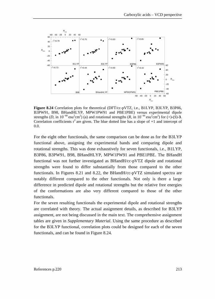
Carboxylic acids – VCD perspective
References p.220 213
-60
-40
-20
0
20
40
60-60 -40 -20 0 20 40 60
B1LYP B3P86B3LYP
Rtheo
B3PW91
r2=0.73
r2=0.78r2=0.75 r2=0.63 r2=0.65
r2=0.42r2=0.60
PBE1PBEMPW1PW91BHandHLYPB98
r2=0.44
-60 -40 -20 0 20 40 60-60
-40
-20
0
20
40
60
Rexp
Rexp
Rtheo
Figure 8.24 Correlation plots for theoretical (DFT/cc-pVTZ, i.e., B1LYP, B3LYP, B3P86, B3PW91, B98, BHandHLYP, MPW1PW91 and PBE1PBE) versus experimental dipole strengths (D, in 10−40 esu2cm2) (a) and rotational strengths (R, in 10−44 esu2cm2) for (+)-(S)-3. Correlation coefficients r2 are given. The blue dotted line has a slope of +1 and intercept of 0.0. For the eight other functionals, the same comparison can be done as for the B3LYP functional above, assigning the experimental bands and comparing dipole and rotational strengths. This was done exhaustively for seven functionals, i.e., B1LYP, B3P86, B3PW91, B98, BHandHLYP, MPW1PW91 and PBE1PBE. The BHandH functional was not further investigated as BHandH/cc-pVTZ dipole and rotational strengths were found to differ substantially from those compared to the other functionals. In Figures 8.21 and 8.22, the BHandH/cc-pVTZ simulated spectra are notably different compared to the other functionals. Not only is there a large difference in predicted dipole and rotational strengths but the relative free energies of the conformations are also very different compared to those of the other functionals. For the seven resulting functionals the experimental dipole and rotational strengths are correlated with theory. The actual assignment details, as described for B3LYP assignment, are not being discussed in the main text. The comprehensive assignment tables are given in Supplementary Material. Using the same procedure as described for the B3LYP functional, correlation plots could be designed for each of the seven functionals, and can be found in Figure 8.24.

Chapter 8
214
The dipole strengths are predicted in good agreement with experiment for all eight functionals, which all perform equally well. This can be seen in Figure 8.24, with correlation coefficients near 90%. For the rotational strengths the situation is different. There is an extra dimension when discussing rotational strengths, i.e., its sign, which can be positive, negative (or zero). Wrongly predicted, this would lead to false conclusions when e.g. elucidating conformational populations or absolute configurations. In Figure 8.24 the correlation plots for the rotational strengths are given for the eight functionals. Based on the correlation, three functionals that are significantly better than the rest can immediately be identified, i.e., B1LYP, B3LYP and B98, with correlation coefficients higher than 70%. On the other end, the BHandHLYP and PBE1PBE have a correlation less than 50%. The other three functionals, i.e., B3P86, B3PW91 and MPW1PW91 are in between with a correlation between 60% and 65%. If the plots are studied in more detail, it can be seen that for four functionals rotational strengths are predicted with the wrong sign. The band assigned as 28XV/29/30TX is predicted with the wrong sign for the B1LYP and B3LYP and for mode 23, the B3LYP the rotational strength is also predicted wrongly. However, there the absolute value of the predicted and experimental rotational strengths is rather low. For the BHandHLYP functional the predicted rotational strength for the band assigned as 24/25/26/27 has a value near 23 which contrasts with the experimental value of approximately −23. For the PBE1PBE functional, the same experimental band is assigned as 25/26/27 (mode 24 is predicted with a lower frequency) and gives the same difference as for BHandHLYP, and additionally mode 22/23W is predicted wrongly. For the other three functionals all rotational strengths are predicted with the correct sign. Another approach to compare experimental and simulated spectra is the use of similarity descriptors.17 Although the theoretical frequencies are scaled linearly to correct for the harmonic approximation and basis set incompleteness, some bands can still be shifted with respect to their corresponding experimental band. A good similarity measure should therefore take into account the neighborhood in direct proximity of the compared points. Also interesting would be the incorporation of the specific frequency scaling of the simulated spectrum in the similarity measure. This scaling factor is dependent on the applied functional and basis set. The functional dependence on the calculated frequency is illustrated in Figures 8.21 and 8.22, where all simulated spectra were scaled with a factor 0.98 which is in general a good value for B3LYP/cc-pVTZ frequencies.
Carboxylic acids – VCD perspective
References p.220 215
The neighborhood similarity (NS) measure that is used in this paper is given in Equation (8.4)
( ) ( )
( ) ( ) ( ) ( )
fg fg
ff ff gg gg
w r c r drS
w r c r dr w r c r dr
σσ
σ σ=
∫∫ ∫
(8.4)
In this similarity descriptor, a weighting function w(r) is introduced to extract the similarity information concerning neighborhoods. For this purpose a triangular function is used as introduced by De Gelder et al.74,
( ) 1
( ) 0
rw r r l
lw r r l
= − ⇔ <
= ⇔ ≥ (8.5)
For our purposes the window size l = 40 cm−1 is chosen, as this gives good results when comparing IR spectra.
( )fgc rσ and ( )ffc rσ are called respectively auto- and cross-correlation functions and are
defined as
( ) ( ) ( )
( ) ( ) ( )
fg
ff
c r f v g v r dv
c r f v f v r dv
σ
σ
σ
σ
= +
= +
∫∫
(8.6)
A scaling factor σ is introduced to consider the scaling between theoretical and experimental spectrum respectively represented by f(ν) and g(ν). The scaling factor that gives the highest similarity can be found by optimizing Sσ in function of σ. In Table 8.10, the maximized NS is given comparing experimental and DFT/cc-pVTZ simulated IR spectra. It can be seen that B3LYP gives a scaling factor closest to unity. The BHandH and BHandHLYP vibrational frequencies are notably more overestimated, yielding scaling factors of respectively 0.90 and 0.92. The simulated IR and VCD spectra for the different functionals with scaled frequencies according to Table 8.10 are given in Figure S8.5 and Figure S8.6 in Supplementary Material. These scaling factors are now used for the calculation of the NS between experimental and simulated VCD for the compound with known absolute configuration. The NS, i.e., Sσ values for each functional are represented in Figure

Chapter 8
216
8.25 in gray. The same can also done for the simulated spectra for the opposite enantiomer, i.e., (R)-3. These NS are also given in Figure 8.25, in black. Table 8.10 Maximized NS for experimental and simulated IR spectrum (DFT/cc-pVTZ) optimized by theoretical frequency scaling. The scaling factor σ gives the optimum, for l = 40 cm−1.
Sσmax σ B1LYP 84.4 0.97 B3LYP 82.6 0.98 B3P86 84.6 0.96 B3PW91 83.2 0.96 B98 84.0 0.97 BHandH 81.0 0.90 BHandHLYP 87.6 0.92 MPW1PW91 83.9 0.95 PBE1PBE 83.0 0.95
Figure 8.25 NS Sσ between experimental (+)-3 and DFT/cc-pVTZ (i.e., functionals B1LYP, B3LYP, B3P86, B3PW91, B98, BHandH, BHandHLYP, MPW1PW91 and PBE1PBE) simulated spectra for the S (correct) and R enantiomer. The applied scaling factors are those from Table 8.10. In gray, the NS between experiment and simulated spectrum for the known correct absolute configuration (S), in black the NS between experiment and the opposite enantiomer (wrong absolute configuration, i.e., (R)), and in white the difference in S/R NS.
76.6
75.3
55.8
54.1
65.2
44.4
65.5
50.4
45.7
52.6
50.6
26.0
25.5
41.3
40.1
20.4
13.6
29.8
28.6
24.0
24.7
23.9
40.0
25.4 30
.0 32.1
4.4
0.0
10.0
20.0
30.0
40.0
50.0
60.0
70.0
80.0
90.0
100.0
B1L
YP
B3L
YP
B3P
86
B3P
W91
B98
BH
andH
BH
andH
LYP
MP
W1P
W91
PBE
1PB
E
Sσ (+) ↔ (S)-3 Sσ (+) ↔ (R)-3
ΔSσ(S)/(R)

Carboxylic acids – VCD perspective
References p.220 217
It can be seen that for the B3LYP and B1LYP functionals a Sσ of 75% and higher can be found when evaluating the correct enantiomer. Except for the BHandH and PBE1PBE functionals that give a Sσ around 45%, the remainder functionals give a similarity between 50 and 66%. Evaluation of the opposite enantiomer gives much lower Sσ, with values between 20 and 30%. The PBE1PBE NS is 32%, and BHandH is an outlier, having a value of 40%. Rather than looking at the absolute values of the NS, it seems more interesting to consider the differences in Sσ evaluated for opposite enantiomers, which are also represented in Figure 8.25 using outlined-white bars. The largest differences in Sσ can be found for the B1LYP, B3LYP, B98 and BHandHLYP. The remaining functionals, i.e., PBE1PBE and BHandH gives the smallest difference in Sσ, with an extreme small difference of 4.4% for the BHandH functional. B3P86, B3PW91 and MPW1PW91 give intermediate ΔSσ values. When comparing these findings to the correlation coefficients in Figure 8.24 it can be observed that the functionals yielding high Rexp/Rtheo correlation coefficients also display the largest differential S/R Sσ. The same trend for functionals with lower correlation coefficients can be observed. Earlier in this paper, the cc-pVTZ/BHandH spectra were found to be notably different compared to spectra produced using other functionals. The BHandH ΔSσ indicate that the visually observed differences are well reflected in the proposed similarity measure. This could indicate that the difference in Sσ evaluated for the correct and wrong enantiomer could be a useful measure for the quality of the agreement between experimental and theoretical VCD spectra. Comparing experimental and theoretical rotational strengths is still superior, giving much more information about the agreement. An example which makes this clear is the discrepancy that can be observed for the BHandHLYP functionals, yielding a somewhat higher differential Sσ than expected from its Rexp/Rtheo correlation. The cc-pVTZ/BHandHLYP predicted rotational strength for band 24/25/26/27 was predicted with the wrong sign yielding a lower correlation, which can not be deduced based on the differential similarity measure. The differential Sσ is still lower compared to the better performing functionals. However, the assignment and extraction of experimental rotational strengths is very labor intensive. A transparent measure for the agreement, such as the calculation of similarities is undemanding and straightforward and would be desirable. To verify the validity of the proposed quality measure, other compounds should be thoroughly tested.
Chapter 8
218
8.4.5 Conclusion
Based on a thorough conformational search performed at DFT/6-31G* level it could be observed that the 6-31G* basis set is unable to describe the PES unambiguously for (S)-3, as the number of minima and the relative energies were particularly functional dependent. The cc-pVTZ conformational description, however, gave a uniform conformational picture over all applied functionals. IR and VCD spectra were simulated using this large cc-pVTZ basis set and nine hybrid functionals, calculating dipole and rotational strengths for each located minimum. Based on both measures, that is, the correlation between experimental and theoretical rotational strengths and the newly introduced differential S/R neighborhood similarities, it can be seen that three functionals perform very good in predicting rotational strengths for 3 applying the cc-pVTZ basis set. B1LYP, B3LYP and B98 give the highest Rexp/Rtheo correlations and largest differential S/R neighborhood similarities. The B3PW91, B3P86 and MPW1PW91 also perform very well, but giving intermediate Rexp/Rtheo correlations. The intermediate performance is also illustrated by the differential neighborhood similarity. The BHandHLYP and PBE1PBE give the lowest Rexp/Rtheo correlations mainly due to the wrongly predicted rotational strengths for an intense band. All tested functionals are found capable of predicting rotational strengths for 3, except the BHandH functional. The reliability of B1LYP, B3LYP, and B98 rotational strengths is higher than for B3P86, B3PW91, BHandLYP, PBE1PBE and MPW1PW91. 8.4.6 Supplementary material index
For this paragraph Supplementary Material is provided. It can be downloaded from http://www.quantum.UGent.be/tksup.pdf Table S8.6 DFT/6-31G* conformational description 3 Table S8.7 DFT/cc-pVTZ fundamental assignment tables Figure S8.5 Simulated (S)-(+)-1 IR DFT/cc-pVTZ spectra for different functionals and experimental spectrum. Figure S8.6 Simulated (S)-(+)-1 VCD DFT/cc-pVTZ spectra for different functionals and experimental spectrum.

Carboxylic acids – VCD perspective
References p.220 219
8.5 Summary
In this chapter, two chiral carboxylic acid compounds and a methyl-ester derivative were studied with the aid of VCD spectroscopy and DFT calculations. The formation of stable carboxylic acid cyclic dimers has a large influence on the vibrational properties of carboxylic acids, which was clearly visible in the vibrational spectra. A wealth of information could be obtained by measuring the IR, but more important, the VCD, because of its conformational sensitivity and differential nature. By modeling the dimer conformations, and simulating IR and VCD spectra, these experimental spectra could be interpreted. For compound 1 it could be established that next to cyclic dimers, also monomers are present at the concentration range that was studied. For compound 2, monomer concentrations were found to be low, and spectra could be simulated on the basis of cyclic dimer conformations. The absolute configuration of this compound was assigned this way. The reason for compound 1, that the monomer concentrations in solution are higher compared to compound 2, is because of the stabilizing intra-molecular hydrogen bonding for a number of monomers. Compound 3, the methyl-ester of compound 1, was studied and it was shown that a simple esterification can eliminate the self-association difficulties. This compound was thoroughly analyzed, applying different density functionals. The reliability of the B1LYP, B3LYP and B98 functionals was found the highest for the calculation of rotational strengths. Additionally, a new method for the evaluation of the agreement between experimental and simulated spectra was introduced, i.e., the differential S/R neighborhood similarity. This measure looks very promising and will be the main topic of the last chapter.
Chapter 8
220
8.6 Reference list
1. Kollman, P. A.; Allen, L. C. Chem. Rev. 1972, 72, 283-303.
2. Patai, S. The Chemistry of acid derivatives; Wiley: New York, 1992.
3. Wolfs, I.; Desseyn, H. O. J. Mol. Struc. (THEOCHEM) 1996, 360, 81-97.
4. He, J. T.; Polavarapu, P. L. J. Chem. Theory Comput. 2005, 1, 506-514.
5. He, J. T.; Polavarapu, P. L. Spectrochim. Acta A 2005, 61, 1327-1334.
6. Fujima, Y.; Hirayama, Y.; Ikunaka, M.; Nishimoto, Y. Tetrahedron-Asymmetr. 2003, 14, 1385-1391.
7. Ishigura, M.; Nishihara, T.; Tanaka, R. Yakugaku Zasshi 2001, 121, 915-927.
8. Hoffman-Roberts, H. L.; Babcock, E. C.; Mitropoulos, I. F. Expert Opin. Invest. Drugs 2005, 14, 973-995.
9. Ayers, P. W.; Yang, W. Density-functional theory. In Computational medicinal chemistry for drugs discovery, Bultinck, P., De Winter, H., Langenaeker, W., Tollenaere, J. P., Eds.; Marcel Dekker, Inc.: New York, 2004; pp 89-118.
10. Cheeseman, J. R.; Frisch, M. J.; Devlin, F. J.; Stephens, P. J. Chem. Phys. Lett. 1996, 252, 211-220.
11. Devlin, F. J.; Stephens, P. J.; Cheeseman, J. R.; Frisch, M. J. J. Phys. Chem. A 1997, 101, 9912-9924.
12. Stephens, P. J.; Ashvar, C. S.; Devlin, F. J.; Cheeseman, J. R.; Frisch, M. J. Mol. Phys. 1996, 89, 579-594.
13. Aamouche, A.; Devlin, F. J.; Stephens, P. J. J. Am. Chem. Soc. 2000, 122, 2346-2354.
14. Devlin, F. J.; Stephens, P. J.; Scafato, P.; Superchi, S.; Rosini, C. Tetrahedron-Asymmetr. 2001, 12, 1551-1558.
15. Dyatkin, A. B.; Freedman, T. B.; Cao, X. L.; Dukor, R. K.; Maryanoff, B. E.; Maryanoff, C. A.; Matthews, J. M.; Shah, R. D.; Nafie, L. A. Chirality 2002, 14, 215-219.

Carboxylic acids – VCD perspective
221
16. Kuppens, T.; Langenaeker, W.; Tollenaere, J. P.; Bultinck, P. J. Phys. Chem. A 2003, 107, 542-553.
17. Kuppens, T.; Vandyck, K.; Van der Eycken, J.; Herrebout, W.; van der Veken, B. J.; Bultinck, P. J. Org. Chem. 2005, 70, 9103-9114.
18. Wang, F.; Polavarapu, P. L. J. Phys. Chem. A 2000, 104, 1822-1826.
19. Stephens, P. J. Vibrational circular dichroism spectroscopy: A new tool for the stereochemical characterization of chiral molecules. In Computational medicinal chemistry for drugs discovery, Bultinck, P., De Winter, H., Langenaeker, W., Tollenaere, J. P., Eds.; Marcel Dekker, Inc.: New York, 2004; pp 699-725.
20. Nafie, L. A. Appl. Spectrosc. 2000, 54, 1634-1645.
21. Kuppens, T.; Bultinck, P.; Langenaeker, W. Drug Discovery Today: Techn. 2004, 1, 269-275.
22. Lewell, X. Q.; Hillier, I. H.; Field, M. J.; Morris, J. J.; Taylor, P. J. J. Chem. Soc. Faraday Trans. II 1988, 84, 893-898.
23. Devlin, F. J.; Stephens, P. J. J. Am. Chem. Soc. 1999, 121, 7413-7414.
24. Wang, F.; Polavarapu, P. L.; Lebon, F.; Longhi, G.; Abbate, S.; Catellani, M. J. Phys. Chem. A 2002, 106, 12365-12369.
25. Cappelli, C.; Corni, S.; Mennucci, B.; Cammi, R.; Tomasi, J. J. Phys. Chem. A 2002, 106, 12331-12339.
26. Wang, F.; Polavarapu, P. L. J. Phys. Chem. A 2000, 104, 10683-10687.
27. Urbanova, M.; Setnicka, V.; Devlin, F. J.; Stephens, P. J. J. Am. Chem. Soc. 2005, 127, 6700-6711.
28. Cervinka, O.; Bajanzulyn, O.; Fabryova, A.; Sackus, A. Collect. Czech. Chem. Commun. 1986, 51, 404-407.
29. Urbanova, M.; Setnicka, V.; Volka, K. Chirality 2000, 12, 199-203.
30. Spectrogon AB, Taeby, Sweden - www.spectrogon.com
31. Aamouche, A.; Devlin, F. J.; Stephens, P. J.; Drabowicz, J.; Bujnicki, B.; Mikolajczyk, M. Chem.-Eur. J. 2000, 6, 4479-4486.

Chapter 8
222
32. Frisch, M. J.; Trucks, G. W.; Schlegel, H. B.; Scuseria, G. E.; Robb, M. A.; Cheeseman, J. R.; Montgomery Jr, J. A.; Vreven, T.; Kudin, K. N.; Burant, J. C.; Millam, J. M.; Iyengar, S. S.; Tomasi, J.; Barone, V.; Mennucci, B.; Cossi, M.; Scalmani, G.; Rega, N.; Petersson, G. A.; Nakatsuji, H.; Hada, M.; Ehara, M.; Toyota, K.; Fukuda, R.; Hasegawa, J.; Ishida, M.; Nakajima, T.; Honda, Y.; Kitao, O.; Nakai, H.; Klene, M.; Li, X.; Knox, J. E.; Hratchian, H. P.; Cross, J. B.; Bakken, V.; Adamo, C.; Jaramillo, J.; Gomperts, R.; Stratmann, R. E.; Yazyev, O.; Austin, A. J.; Cammi, R.; Pomelli, C.; Ochterski, J. W.; Ayala, P. Y.; Morokuma, K.; Voth, G. A.; Salvador, P.; Dannenberg, J. J.; Zakrzewski, V. G.; Dapprich, S.; Daniels, A. D.; Strain, M. C.; Farkas, O.; Malick, D. K.; Rabuck, A. D.; Raghavachari, K.; Foresman, J. B.; Ortiz, J. V.; Cui, Q.; Baboul, A. G.; Clifford, S.; Cioslowski, J.; Stefanov, B. B.; Liu, G.; Liashenko, A.; Piskorz, P.; Komaromi, I.; Martin, R. L.; Fox, D. J.; Keith, T.; Al-Laham, M. A.; Peng, C. Y.; Nanayakkara, A.; Challacombe, M.; Gill, P. M. W.; Johnson, B.; Chen, W.; Wong, M. W.; Gonzalez, C.; Pople, J. A. Gaussian03, Revision B5; Gaussian, Inc.: Wallingford CT, 2004.
33. Becke, A. D. J. Chem. Phys. 1993, 98, 5648-5652.
34. Lee, C. T.; Yang, W. T.; Parr, R. G. Phys. Rev. B-Condens. Matter 1988, 37, 785-789.
35. Stephens, P. J.; Devlin, F. J.; Chabalowski, C. F.; Frisch, M. J. J. Phys. Chem.-US 1994, 98, 11623-11627.
36. Sander, W.; Gantenberg, M. Spectrochim. Acta A 2005, 62, 902-909.
37. Sadlej, J.; Dobrowolski, J. C.; Rode, J. E.; Jamroz, M. H. Phys. Chem. Chem. Phys. 2006, 8, 101-113.
38. Frisch, A. E.; Frisch, M. J.; Trucks, G. Gaussian 03 User's Reference; 5th
ed.; Gaussian, Inc.: Pittsburgh, 2003.
39. Ditchfield, R. Mol. Phys. 1974, 27, 789-807.
40. Stephens, P. J. J. Phys. Chem.-US 1987, 91, 1712-1715.
41. McQuarrie, D. A. Statistical Thermodynamics; Harper and Row: New York, 1973.
42. Hehre, W. J.; Radom, L.; Schleyer, P. R.; Pople, J. A. Ab initio molecular orbital theory; Wiley: 1986.
Carboxylic acids – VCD perspective
223
43. Allinger, N. L.; Yuh, Y. H.; Lii, J. H. J. Am. Chem. Soc. 1989, 111, 8551-8566.
44. Allinger, N. L.; Chen, K. S.; Lii, J. H. J. Comput. Chem. 1996, 17, 642-668.
45. Halgren, T. A. J. Comput. Chem. 1996, 17, 490-519.
46. Cremer, D.; Pople, J. A. J. Am. Chem. Soc. 1975, 97, 1354-1358.
47. Wu, A.; Cremer, D. J. Phys. Chem. A 2003, 107, 1797-1810.
48. Fernandez, L. E.; Marigliano, A. C. G.; Varetti, E. L. Vib. Spectrosc. 2005, 37, 179-187.
49. Eliason, T. L.; Havey, D. K.; Vaida, V. Chem. Phys. Lett. 2005, 402, 239-244.
50. Kuppens, T.; Herrebout, W.; van der Veken, B. J.; Corens, D.; De Groot, A.; Doyon, A.; Van Lommen, G.; Bultinck, P. Chirality 2006, 18, 609-620.
51. Yu, Y. B.; Privalov, P. L.; Hodges, R. S. Biophys. J. 2001, 81, 1632-1642.
52. Chen, J. S.; Wu, C. C.; Kao, D. Y. Spectrochim. Acta A 2004, 60, 2287-2293.
53. Zhao, C. X.; Polavarapu, P. L. Biospectroscopy 1999, 5, 276-283.
54. Antony, J.; von Helden, G.; Meijer, G.; Schmidt, B. J. Chem. Phys. 2005, 123, 014305
55. Janssens, F. E.; Sommen, F.; De Boeck, B.; Benoit, C.; Leenaerts, J. E. WO A2 2004056799, 2003.
56. Nafie, L. A. Appl. Spectrosc. 1996, 50, A14-A26.
57. Stephens, P. J.; Devlin, F. J. Chirality 2000, 12, 172-179.
58. Freedman, T. B.; Cao, X. L.; Dukor, R. K.; Nafie, L. A. Chirality 2003, 15, 743-758.
59. Bélanger, P. C.; Williams, H. W. R. Can. J. Chem. 1983, 61, 1383-1386.
60. Freedman, T. B.; Cao, X. L.; Oliveira, R. V.; Cass, Q. B.; Nafie, L. A. Chirality 2003, 15, 196-200.

Chapter 8
224
61. Setnicka, V.; Urbanova, M.; Bour, P.; Kral, V.; Volka, K. J. Phys. Chem. A 2001, 105, 8931-8938.
62. Woon, D. E.; Dunning, T. H. J. Chem. Phys. 1993, 98, 1358-1371.
63. Kendall, R. A.; Dunning, T. H.; Harrison, R. J. J. Chem. Phys. 1992, 96, 6796-6806.
64. Wong, M. W. Chem. Phys. Lett. 1996, 256, 391-399.
65. Scott, A. P.; Radom, L. J. Phys. Chem.-US 1996, 100, 16502-16513.
66. Wang, F.; Polavarapu, P. L. J. Phys. Chem. A 2000, 104, 6189-6196.
67. McCann, J. L.; Rauk, A.; Wieser, H. Can. J. Chem. 1998, 76, 274-283.
68. Nevins, N.; Chen, K. S.; Allinger, N. L. J. Comput. Chem. 1996, 17, 669-694.
69. Cremer, D.; Pople, J. A. J. Am. Chem. Soc. 1975, 97, 1358-1367.
70. Ashvar, C. S.; Devlin, F. J.; Bak, K. L.; Taylor, P. R.; Stephens, P. J. J. Phys. Chem.-US 1996, 100, 9262-9270.
71. Buffeteau, T.; Ducasse, L.; Brizard, A.; Huc, I.; Oda, R. J. Phys. Chem. A 2004, 108, 4080-4086.
72. Schellman, J. A. Chem. Rev. 1975, 75, 323-331.
73. He, J. T.; Petrovich, A.; Polavarapu, P. L. J. Phys. Chem. A 2004, 108, 1671-1680.
74. De Gelder, R.; Wehrens, R.; Hageman, J. A. J. Comput. Chem. 2001, 22, 273-289.

References p.242 225
Equation Chapter 9 Section 1
9 neighborhood based
enantiomeric
similarity index
9.1 Introduction
The reliability of AC determinations using the VCD methodology unmistakably depends on the quality of the experimental data and the performance of the DFT calculations. If the compounds provided are enantiomerically pure and the VCD baseline correction can be performed, the obtained spectra should be of very high quality. This is not always the case, however. Samples of chiral compounds can contain small concentrations of impurities and the compounds can also have a lower or unknown enantiomeric excess. Racemic mixtures or both enantiomers are not always available, which ultimately results in less accurate baselines. At the other

Chapter 9
226
end, basis set size, choice of density functional, numerical integration grid size, etc. can have an influence on the usability of the simulated spectra. In addition, if an important conformation is not found during the conformational search, this would a major pitfall. Taking into account the argumentation from above, the following question can be raised: What is the reliability of an AC assignment using the VCD methodology and can one quantify the quality of an assignment? Up until now, very few studies are published that discus the criteria to assess whether a reliable prediction can be made. In Reference 1, D. Minick explains the quality assessment at GlaxoSmithKline; “The key to confident predictions at GSK is the value of the […] coefficients of correlation between the intensities of 10–15 corresponding bands in the calculated and measured spectra. Our assignments are considered reliable if r2 is at least 90%”. In Chapter 4 it was already established that there are different ways to quantify the agreement between the experimental and simulated spectra. The most reliable method, but very time consuming and not transparent, is to determine the correlation between experimental and theoretical rotational strengths. A neighborhood similarity measure was introduced that allows a more transparent quantification of the agreement. The central problem in AC determination is the capacity to distinguish between two enantiomers.2 A new quantity was therefore introduced (see §8.3) on the basis of neighborhood similarity, in which the agreement is assessed between the experimental VCD and the simulated spectra of both enantiomers. Only one compound was tested using this differential neighborhood similarity measure (methyl tetrahydrofuran-2-carboxylate).3 In this chapter, the main objective is to test the differential neighborhood similarity measure for its applicability in enantiomeric discrimination and whether it can be used to quantify the confidence of an assignment. First, a comprehensive overview is given of this newly proposed quantity and new terminology and symbols are introduced. In what follows, a set of 21 compounds is presented that will be used for the evaluation of the proposed neighborhood similarity measure.

Enantiomeric similarity index
References p.242 227
9.2 Enantiomeric similarity index
The neighborhood similarity (NS) was introduced in Chapter 4 in Equation (4.17). This similarity measure does not only takes into account the overestimation of the calculated frequencies via a scaling factor σ, but also deals with the local shift of bands. The latter is done using correlation functions and a triangular weighting function. Equation (4.17) is for convenience reintroduced in this chapter,
( ) ( )
( ) ( ) ( ) ( )
fg fg
ff ff gg gg
w r c r drS
w r c r dr w r c r dr
σσ
σ σ=
∫∫ ∫
(9.1)
with
( ) 1
( ) 0
rw r if r l
lw r if r l
= − <
= ≥ (9.2)
and the correlation functions defined as
( ) ( ) ( )fgc r f g r dσ σν ν ν= +∫ (9.3)
The NS is a quantity within the interval [0, 1]. The optimization of S σ is carried out by searching the optimal σ through scaling of the vibrational frequencies of the theoretical spectrum ( )f ν . When evaluating S σ for corresponding IR and VCD data, their maximizing scaling factor σopt is slightly different, in the order of 1 or 2%. This difference is expected, as the S/N ratio in the VCD spectra is considerably higher than in the IR. Therefore, the scaling factor for theoretical frequency scaling we use, is determined by optimizing S σ for the experimental and theoretical IR spectra. The latter is denoted by max(IR)S σ and the scaling factor is abbreviated as σopt,IR. In the same way, max(VCD)S σ and σopt,VCD can be defined. For VCD purposes, ( )f ν can be defined as the perfect mirror image spectrum of ( )f ν . From a more practical approach it can be said that if ( )f ν represents the

Chapter 9
228
spectrum of modeled compound and ( )f ν represents the simulated spectrum of the
opposite enantiomer. (VCD)S σ and (VCD)Sσ can be calculated for respectively
( )f ν and ( )f ν and the experimental spectrum ( )g ν for a specific scaling factor. If
the frequencies of ( )f ν and ( )f ν are both scaled with σopt,IR, (VCD)S σ and
(VCD)Sσ give a measure for the agreement between the experimental VCD and the
simulated VCD spectra for both enantiomers separately. (VCD)S σ and (VCD)Sσ
with σ = σopt,IR will be denoted further respectively as V and V , the VCD NS. If it is assumed now, that the measurement and simulation of the spectra can be regarded as reliable, the simulated VCD spectrum for one enantiomer should have a good agreement with the experimental VCD, whilst the spectrum of the opposite enantiomer should hardly show any agreement, that is, should have intensities with opposite sign. This is the basis of the enantiomeric discrimination potential of VCD. This should consequently be reflected in the values of the VCD NS, i.e., V and V ; one should be significantly lower than the other. The difference between both VCD NS, that is, VΔ is defined as the enantiomeric similarity index (ESI), V V VΔ = − (9.4) The ESI is limited to the interval [−1, 1]. A positive ESI indicates that ( )f ν has a
better agreement with ( )g ν , a negative ESI signifies that ( )f ν has a better agreement with ( )g ν . The absolute value of VΔ gives a measure for the enantiomeric discrimination power. High absolute values of VΔ indicate that one of the enantiomeric spectra has a significantly better agreement with the experimental spectrum ( )g ν compared to the other. Low absolute values give no information and
indicate that both ( )f ν and ( )f ν have a comparable agreement with ( )g ν . In the next section, the newly proposed ESI will be screened for its applicability and validity using a set of 21 compounds. 9.3 Results
In Figure 9.1 and Table 9.1 an overview of the set of 21 compounds is given which are utilized to test the functionality and validity of the ESI. For each compound the conformational behavior was thoroughly studied, and IR and VCD spectra were

Enantiomeric similarity index
References p.242 229
simulated at different levels of theory. For most compounds these details can be found in the previous chapters. Compounds (e),(m)–(s) are not discussed in detail in this dissertation, but spectra and additional information can be found in the Appendix. Details of compounds (i)–(l) were not integrated in this thesis, but can be found in Reference 4. An overview of references is provided in Table 9.1. Except for compounds (a),(g),(m)–(s), all the experimental spectra were measured ourselves.
HOOH HOO OO
O
O
OH
OAc
AcO HO
OH TfO
OTf
O
O
N
O
OOH
HNN
O
N
CH2ClCl2HC
CHCl2
ClCl
Cl
Cl
ClO
O
OH
OO
FNO2
NN
S
N
NHCl
O
OH
HN
OCH3
NH2
EtOOCCOOEt
HCl
NH2
Cl
Cl
Cl
OH
(a) (b) (c) (d)
(e) (f) (g)
(i) (j)(k) (l)
(m) (n) (o)
(p)
(q)(r)
(s) (t) (u)
O
O
OMe
(h)
Figure 9.1 Overview of the set of compounds that is used to test the enantiomeric similarity index.

Chapter 9
230
Table 9.1 names and labels for the set of compounds given in Figure 9.1, with references. Compound name Reference
a 3-hydroxymethyl-2,3-dihydro-[1,4]dioxino[2,3-b]pyridine
Chapter 5, Ref. 5
b 1,2,3,6,7,8-Hexahydro-as-indacene-1,8-diol Chapter 6, Ref. 6
c 8-Hydroxy-3,6,7,8-tetrahydro-2H-as-indacen-1-one Chapter 6, Ref. 6
d 1,2,7,8-di-epoxy-3,6-dihydro-as-indacene Chapter 6, Ref. 6
e 2,2,3-exo,5-endo,6-exo,8,9,9,10,10-decachlorobornane Appendix, Ref. 7
f tetrahydrofuran-2-carboxylic acid Chapter 8, Ref. 8
g tetrahydrofuran-3-carboxylic acid Chapter 8
h methyl tetrahydrofuran-2-carboxylate Chapter 8, Ref. 3
i bicyclo[3.3.0]octane-2,6-bisacetate Ref. 4
j bicyclo[3.3.0]octane-2,6-diol Ref. 4
k bicyclo[3.3.0]octane-2,6-dion Ref. 4
l bicyclo[3.3.0]octane-2,6-dieen-bisvinylic-triflate Ref. 4
m 3,3-Dimethyl-hexahydro-imidazo[1,5-alpha]pyrazin-1-one
Appendix, Ref. 9
n 1-(6-fluorochroman-2-yl)ethanone Appendix, Refs. 10,11
o 2,3,5,6-tetrahydro-6-(3-nitrophenyl)-imidazo[2,1-b]thiazole
Appendix, Ref. 12
p 1-Chloro-8-ethyl-5,6-dihydro-4-phenyl-4H-pyrrolo[1,2-a][1,4]benzodiazepine
Appendix, Refs. 13,14
q 11-fluoro-3,3a,8,12b-tetrahydro-2H-dibenzo[3,4:6,7]cyclohepta[1,2-b]furan-2-methanol
Appendix, Refs. 15-17
r 3-methoxypiperidin-4-amine Appendix, Refs. 18,19
s diethyl1-phenyl-1,2,3,4-tetrahydronaphthalene-1,4-dicarboxylate
Appendix, Ref. 20
t 1-(3’,4’-dichlorophenyl)-propanamine Chapter 7, Ref. 21
u 1-(3’,4’-dichlorophenyl)-propanol Chapter 7, Ref. 21 For the calculation of the NS, the window size l of the triangular weighting function is taken as 40 cm−1 (see Chapter 4). In Table 9.2, the results for the different descriptors are given for the 21 compounds in our set. Default, the B3LYP functional and the 6-31G* basis set are used. If different basis sets and/or density functionals were used, this is mentioned. For compound (a), various DFT integration

Enantiomeric similarity index
References p.242 231
grids were applied in combination with B3LYP/6-31G* level of theory. If not mentioned, the (75,302)p grid is used. Compounds (f) and (g) are carboxylic acids, and to simulate spectra for these molecules, dimers should be taken into account. More details can be found in Chapter 8. For each simulated spectrum, the maximized IR NS max(IR)S σ with experiment was determined. This yielded the scaling factor (σopt,IR) which was applied to determine the VCD NS between experiment and simulation for both enantiomers, i.e., V and V . Here, ( )f ν was chosen as the spectrum that corresponds to the enantiomer with
the same AC as the measured compound; ( )f ν corresponds with the enantiomer with opposite AC. Table 9.2 NS based descriptors for 21 compounds at different levels of approximation, i.e.,
max(IR)S σ , σopt,IR, V , V and VΔ or ESI (in percent). When not specified, the B3LYP functional with 6-31G* basis set and (75,302)p integration grid is used.
max(IR)S σ σopt,IR V V VΔ
ESI a 6-31G* 95.4 0.969 83.6 12.3 71.3 6-31G** 96.5 0.970 83.6 11.9 71.7 6-311G** 96.4 0.981 85.7 11.5 74.2 cc-pVDZ 96.7 0.977 81.6 15.5 66.1 cc-pVTZ 96.9 0.979 89.7 15.2 74.5 (35,110)p 95.1 0.971 80.4 14.3 66.1 (50,194)p 95.4 0.969 83.4 12.1 71.3 (50,194)p 95.4 0.969 84.0 12.0 72.0 (50,302) 95.4 0.969 83.9 12.3 71.6 (75,194) 95.4 0.969 83.1 12.0 71.1 (75,302)p 95.4 0.969 83.6 12.3 71.3 (75,434) 95.4 0.969 83.3 12.5 70.8 (99,302) 95.7 0.969 83.8 13.5 70.3 b cc-pVTZ 97.2 0.977 79.5 11.8 67.7 B1LYP 93.8 0.955 76.7 14.3 62.4 B3LYP 93.6 0.961 75.6 14.6 61.0 B3P86 90.8 0.944 73.0 26.8 46.2 B3PW91 91.3 0.947 74.5 24.2 50.3 B98 92.8 0.958 79.0 17.1 61.9 BHandH 85.6 0.900 52.2 40.9 11.3 BHandHLYP 91.4 0.908 75.7 21.8 53.9 MPW1PW91 90.6 0.936 71.9 27.8 44.1 PBE1PBE 90.4 0.928 61.8 34.9 26.9 c cc-pVTZ 93.9 0.966 80.7 11.9 68.8 B1LYP 91.3 0.945 73.6 11.9 61.7 B3LYP 92.0 0.952 74.3 12.4 61.9 B3P86 91.7 0.942 62.6 14.7 47.9 B3PW91 91.6 0.943 62.9 14.9 48.0 B98 89.4 0.944 64.6 13.8 50.8 BHandH 59.4 1.063 23.0 44.2 −21.2 BHandHLYP 87.1 0.900 62.4 14.8 47.6

Chapter 9
232
MPW1PW91 91.1 0.932 59.4 16.0 43.4 PBE1PBE 90.8 0.931 56.6 17.3 39.3 d cc-pVTZ 94.6 0.975 80.8 19.9 60.9 B1LYP 89.5 0.957 63.3 26.5 36.8 B3LYP 89.8 0.963 66.2 25.7 40.5 B3P86 90.4 0.964 64.9 20.8 44.1 B3PW91 90.4 0.964 65.0 21.5 43.5 B98 91.5 0.967 68.2 25.8 42.4 BHandH 87.0 0.934 55.9 22.8 33.1 BHandHLYP 87.9 0.927 48.2 26.8 21.4 MPW1PW91 89.9 0.959 60.9 21.5 39.4 PBE1PBE 89.7 0.962 60.5 20.0 40.5 e 91.7 0.998 75.6 44.7 30.9 f 6-31++G** 90.3 0.983 76.0 26.4 49.6 aug-cc-pVTZ 87.2 0.976 84.1 22.3 61.8 g 6-31++G** 93.8 0.967 51.1 46.5 4.6 h B1LYP 84.4 0.968 76.6 24.0 52.6 B3LYP 82.6 0.975 75.3 24.7 50.6 B3P86 84.6 0.960 55.8 29.8 26.0 B3PW91 83.2 0.962 54.1 28.6 25.5 B98 84.0 0.966 65.2 23.9 41.3 BHandH 81.0 0.904 44.4 40.0 4.4 BHandHLYP 87.6 0.920 65.5 25.4 40.1 MPW1PW91 83.9 0.951 50.4 30.0 20.4 PBE1PBE 83.0 0.950 45.7 32.1 13.6 i (RRSR) 75.3 0.980 57.9 29.7 28.2 i (RSSS) 75.3 0.978 52.8 39.8 13.0 i (RSSR) 75.1 0.980 59.0 31.9 27.1 i (SSSS) 75.6 0.977 32.7 52.6 −19.9 j (SRRS) 95.4 0.967 76.8 25.3 51.5 j (SRRR) 91.7 1.037 45.4 25.7 19.7 j (RRRR) 88.3 1.044 34.3 28.2 6.1 j (RRSR) 86.1 1.013 24.3 40.5 −16.2 k 92.5 0.945 56.1 32.6 23.5 l 81.1 0.966 78.0 20.1 57.9 m 6-31G* 87.0 0.931 40.2 30.1 10.1 cc-pVTZ 94.6 0.989 74.4 23.6 50.8 n 78.7 0.968 78.6 15.0 63.6 o 6-31G* 79.4 0.949 65.4 43.9 21.5 cc-pVTZ 82.8 0.965 68.5 29.1 39.4 p 95.9 0.971 88.2 36.5 51.7 q 6-31G* 94.1 0.965 82.4 22.3 60.1 cc-pVTZ 96.3 0.976 86.4 25.2 61.2 r 97.8 0.963 77.1 39.0 38.1 s 96.9 0.983 79.0 17.2 61.8 t cc-pVTZ 93.1 0.978 85.1 12.3 72.8 u cc-pVTZ 93.1 0.979 90.3 13.0 77.3

Enantiomeric similarity index
References p.242 233
9.3.1 Scaling factor
In this approach, the IR NS global maximum is determined by scaling the calculated frequencies. From Table 9.2, the influence of the basis set size on the calculated frequencies becomes immediately clear through the IR scaling factor. For larger basis sets the scaling factor is closer to unity than for smaller basis sets. The applied functional even has a larger influence on the calculated frequencies. It can be expected that in some cases over-scaling occurs when aligning the patterns of two spectra. An example is the BHandH/6-31G* spectrum for compound (c). A maximized IR NS is found for a scaling factor of 1.063. A local minimum can be found near σ = 0.955, which is more likely for a frequency scaling factor, with VCD NS of 45.3% and 20.2%. Irregular scaling factors can also be found for the diastereomers for compound (j): the diastereomer that configurationally corresponds to the experimentally measured compound gives a scaling factor of 0.967, whilst the other diastereomers yield substantially higher values all above unity. As can be seen in Figure 9.6, the three diastereomers with the high scaling factors have completely different IR characteristics compared to the configuration SRRS. This will be discussed further in Paragraph 9.3.5. For compound (e) (spectra can be found in the Appendix, Figure A8 and Figure 9.4), it can be seen that uniform frequency scaling sometimes does not work very well, i.e., aligning experimental and theoretical spectra. Using the max(IR)S σ approach, the most intense IR profiles will always be aligned, sometimes without regard for the smaller IR bands. In Paragraph 9.3.4, this will be discussed in more detail. Performing the scaling by maximizing the IR NS is certainly not flawless. It maximizes the neighborhood overlap between two spectra without any chemical correlation. For hybrid functionals the uniform scaling factor is found to reside between 0.9 and 1.0. However, nothing guarantees that the global minimum of
( )S IRσ is found within that range, unless the optimization procedure forces the value of σ to fall within 0.90 and 1.00. In our routine, however, we do not impose this tight restriction, and let σ vary between 0.90 and 1.30. This method gives mostly good results, in cases were experimental and simulated spectra have a good agreement. If the scaling factor is higher than expected, this should give a indication that something could be wrong.

Chapter 9
234
9.3.2 Basis set
The cc-pVTZ basis set is regarded as superior to the smaller 6-31G* basis set when calculating rotational strengths. This does not mean that this smaller basis set is unusable, to the contrary: the 6-31G* basis set provides usable rotational strengths at a much lower computational cost than the cc-pVTZ basis set. The ESI should be able to reflect the basis set effect, i.e., for a certain compound, VΔ should be higher for better performing basis sets. For compound (a), 5 different basis sets were applied in combination with the B3LYP functional. The cc-pVTZ and 6-311G** basis sets gives the highest ESI. The lowest value can be found for the cc-pVDZ basis set, yielding a value lower than the 6-31G* ESI. In Figure 9.2 it can be seen that this is probably due to a underestimated intensity of the positive band near 1240 cm−1.
1600 1500 1400 1300 1200 1100 1000-0.05
-0.04
-0.03
-0.02
-0.01
0.00
0.01
0.02
0.03
0.04 cc-pVTZ 6-31G* cc-pVDZ experiment
Δ ε
ν Figure 9.2 B3LYP spectra for three basis sets (cc-pVTZ, 6-31G* and cc-pVDZ) and experimental VCD. For the other compounds for which cc-pVTZ spectra are available, it can be seen that the obtained VΔ values are all higher than the 6-31G* values. For compound (m) the difference between the 6-31G* and cc-pVTZ is rather large, which is due to the scaling factor 0.931, which is probably too small for the 6-31G* basis set. The quality of the experimental spectra is also somewhat less, which makes the comparison more difficult anyway. The spectra for compound (m) are depicted in Figure A.1 in the Appendix.

Enantiomeric similarity index
References p.242 235
For this set of compounds, it seems that the ESI is able to quantify the performance of the basis sets for the calculation rotational strengths. 9.3.3 Functional
In literature, local, non-local and hybrid functionals, specifically LSDA, BLYP, B3LYP and B3PW9122-26 were mostly studied. Very few explorations of hybrid functionals in the context of VCD simulations are found. Devlin et al. mention very briefly that the B3P86 and B3PW91 functionals “have given extremely similar vibrational spectra”.26 Similarly as for the basis set, the density functionals can evaluated for a given compound. Calculations were performed on four compounds, using a series of hybrid functionals all available in Gaussian03, i.e., B1LYP, B3LYP, B3P86, B3PW91, B98, BHandH, BHandHLYP, MPW1PW91 and PBE1PBE in combination with the 6-31G* basis set. In Figure 9.3 the VΔ values are depicted for the four compounds. Here, it can be seen that B3LYP and B1LYP have very similar values for VΔ . Also B3P86 and B3PW91 perform similar. This is in agreement with the findings of Devlin et al. The remainder of the functionals do not seem to have any mutual correspondence.
Figure 9.3 ESI for different hybrid functionals and 4 compounds. For compound c, the BHandH/6-31G* ESI value is negative (off-scale).
0
10
20
30
40
50
60
70
B1LY
P
B3LY
P
B3P8
6
B3PW
91
B98
BHan
dH
BHan
dHLY
P
MPW
1PW
91
PBE1
PBE
bcdh

Chapter 9
236
In a study performed on compound (h)3, the B3LYP, B1LYP and B98 functionals were found to perform better than the other functionals, based on the correlation between experimental and theoretical rotational strengths. The same conclusion could be formulated based on the ESI, VΔ , also given in Figure 9.3. The only discrepancy found was for the BHandHLYP functional, for which the Rexp/Rtheo correlation coefficient was small (44%) compared to the relatively high value for
VΔ . The BHandH functional was found to yield unusable VCD spectra. For the three other compounds, it can be seen in Figure 9.3 that the B3LYP and B1LYP functionals yield the highest VΔ values. For compound (d), the ESI is more or less 6% lower than the B3P86, B3PW91 and B98 functionals, which yield the highest VΔ values. The BHandH functional clearly gives a low ESI, and for compound (c) VΔ is found to be negative which indicates that the spectrum of the other enantiomer has a higher similarity with the experimental VCD than the spectrum of ‘correct’ enantiomer (actually when using the a local optimum scaling factor of 0.955 an ESI of 25.1% is found). For the other functionals it can be seen that the value for VΔ depends on the compound and not much conclusions can be drawn from these data. Based on the ESI, it could be concluded that the B3LYP and B1LYP functionals perform best in the calculation of rotational strengths. However, more compounds should be processed to generalize this conclusion. 9.3.4 Absolute configuration assignment and quality
For the set of 21 compounds the AC were assigned after thorough analysis (assignment of fundamentals) of the agreement between experimental an simulated IR and VCD spectra. An interesting and still open question is if NS measures, and more precisely the ESI, can be used to assign absolute configurations. If the proposed NS measure, i.e., (VCD)S σ , is reliable enough to quantify the agreement between experimental and simulated VCD spectra, one can argue that this measure can be used to assign the AC of the measured compound. The enantiomer with the highest (VCD)S σ has consequently the same absolute configuration as the measured compound. In this argumentation, of course, it is assumed that theory and experimental spectra are of high quality. Because the spectrum ( )f ν for the 21 compounds tested, was chosen to correspond to the enantiomer having the same AC as the measured compound, each compound in the set should have a positive ESI. If VΔ would be negative, it would mean that

Enantiomeric similarity index
References p.242 237
based on the VCD NS, the spectrum corresponding to the opposite (wrong) enantiomer would have a higher resemblance to the experimental spectrum then ( )f ν , based on the NS measure.
For all compounds, (i) and (j) not included (this is a case of diastereomers and will be discussed further), it can be seen that, for a reliable level of theory, a positive ESI is found. This indicates that the enantiomeric similarity index can indeed be used for an indicator for the assignment of ACs. Some prudence is of course advised: this set only counts 21 compounds and it is not our intention to generalize this conclusion to other compounds without further testing on a larger set. Also, above it was already found that for a better performing basis set, larger values can be found for the enantiomeric similarity index. This was also found more or less for functionals, especially the bad performing (for 4 compounds) BHandH which gives a negative ESI. It is, however, rather difficult to pass a judgment on the quality of the performed experiment. Low S/N ratios and deviating baselines are indicators for spectra with lower reliability. Do these effects show in the ESI for a certain compound? Is the ESI lower when the quality of the spectra is questionable? Compound (e) is modeled at the B3LYP/6-31G* level and has only one significant conformation. This compound has a low VCD signal, and combined with small sample amounts available, the VCD spectrum has a high S/N ratio as can be seen in Figure A8 in the Appendix and Figure 9.4. The VCD baseline was estimated using a racemic mixture. For this compound, a relatively low ESI is observed. One can argue that this low ESI is due to the bad uniform scaling, as mentioned earlier. However, when only the 1100–800 cm−1 region is analyzed, in which experiment and simulation are perfectly aligned with a σopt,IR = 0.999, the ESI only rises 1%, i.e., 31.7%. Another example in which interfering experimental effects occur is solvent-solute or solute-solute interaction. It is not a routine practice to take these kind of effects into account. In case of carboxylic acids it is absolutely necessary to take the intermolecular association into regard as stable dimers can be formed.8,27 For compound (g) (see §8.3), the dimeric spectrum was modeled and compared to the experimental spectrum. Agreement can be seen between experiment and theory when carboxylic acid dimers are considered and assigning fundamentals (Figures 8.16 and 8.17) However, a small ESI is found, i.e., 4.6%. Can we conclude from this value that the reliability from this assignment is not high? Whatever the case may be, the spectra are simulated on the basis of cyclic dimer conformation, not accounting for the monomers. The low ESI may be an indication that monomer

Chapter 9
238
conformation should be accounted for. For compound (f) (see §8.2), also a carboxylic acid, the simulation of the spectra was more elaborated, taking into account dimers and monomers, using semi-qualitative populations. For these simulated spectra an ESI of 49.6% was found.
1100 1050 1000 950 900 850 800-0.03
-0.02
-0.01
0.00
0.01
Δ ε
ν
exp ~g(ν )
-0.03
-0.02
-0.01
0.00
0.01
0.02
0.03
Δ ε
B3LYP/6-31G* ~ f(ν )
Δ ε
-0.03
-0.02
-0.01
0.00
0.01
0.02
0.031100 1050 1000 950 900 850 800
B3LYP/6-31G* ~ f(ν )
Figure 9.4 Experimental ( )g ν and B3LYP/6-31G* simulated spectra ( )f ν and ( )f ν for compound (e) in the 1100–800 cm−1 window. Calculated frequencies were scaled with a factor 0.999. The B3LYP/cc-pVTZ VCD NS for compound (u) are very different from each other, i.e., 90.3% and 13.0%, yielding a ESI of 77.3% In Figure 7.6 the VCD spectra are given. The Rexp/Rtheo correlation coefficient for this compound was determined to be is 91%. Compound (t) has a lower correlation coefficient, i.e., 66%. This lower correlation was attributed to three fundamentals, which lower the correlation (for both dipole and rotational strengths) drastically. If these are discarded a Rexp/Rtheo correlation of 91% can be found. The ESI for this compound is 72.8%. Other compounds for which a correlation was made between experimental and theoretical values of dipole and rotational strengths are compounds (b), (c) and (d) which are structurally related to each other. These compounds have respectively a Rexp/Rtheo correlation coefficient of 53%, 64% and 38% comparing B3LYP/cc-pVTZ

Enantiomeric similarity index
References p.242 239
data to experimental data. From Table 9.2 it can be seen that the ESI for these compounds is respectively 67%, 68% and 60%. Above examples indicate that if the experimental and simulated spectra are of good quality, the ESI is relatively high. If the experimental spectrum has a somewhat lower quality, or the level of theory used is somewhat inferior, the ESI gives lower values. This could indicate that the ESI has the ability to quantify the agreement, i.e., may be used as an indicator for the reliability of the AC assignment. Again, we do not want generalize this conclusion to other compounds and further testing is needed. 9.3.5 Diastereomer assignment
From the above it can be seen that the ESI is a measure that has the potential to discriminate between enantiomers. Can the ESI also be used for diastereomer discrimination?
1800 1700 1600 1500 1400 1300 1200 1100 1000-0.06-0.030.000.030.06
-0.040.000.04
-0.02
0.00
0.02 -0.04
0.00
0.04-0.04
0.00
0.04
exp
Δ εRRSR
RSSS
ν
Δ εRSSR
Δ ε
Δ ε
Δ ε
SSSS
Figure 9.5 Simulated B3LYP/6-31G* VCD spectra for 4 diastereomers and experimental spectrum for compound (i). Theoretical frequencies are scaled with a factor 0.98. For compounds (i) and (j), the different diastereomers were studied. Due the C2 symmetry present in both compounds, there are only 4 optically active isomers. For each compound, the IR and VCD spectra were simulated for all optical active diastereomers. Based on thorough analysis of experimental and simulated spectra

Chapter 9
240
and the assignment of fundamentals, we were able to determine the correct absolute configuration of the compound, i.e., the correct enantiomer and diastereomer for compound (i) and (j).4 In Figures 9.5 and 9.6 the experimental and simulated VCD spectra are given for both compounds and the different diastereomeric configurations. For compound (i), the visual agreement between experiment and the simulated VCD spectra is not very good. The AC for compound (i) was assigned as RSSR.4 The ESI for the RRSR, RSSS, RSSR and SSSS are respectively (Table 9.2) 28.2%, 13.0%, 27.1% and −19.9%. The configurations with the highest ESI are RRSR and RSSR. Configuration RRRR (enantiomer of SSSS, the RRRR spectrum is not shown in Figure 9.5) has a value of 19.9% which is significantly lower. If the spectra of RRSR and RSSR are compared in Figure 9.5 then it seems that the large features are very similar apart from the CO stretch band. Based on their ESI it is not possible to identify the correct configuration for this compound, and a thorough analysis is needed that identifies each band for 1:1 comparison. The ESI measure identifies that the enantiomer of SSSS, that is, RRRR (mirror image VCD spectrum) has a relative good similarity with the experiment. Indeed, the large features near 1250 cm−1 and the CO stretch band of the RRRR VCD spectrum agree with the experimental spectrum (however, differences for smaller bands allows to discard this configuration in the assignment).
1400 1300 1200 1100 1000 900
-0.015-0.010-0.0050.0000.0050.010
-0.010-0.0050.0000.005
-0.003
0.000
0.003
-0.0050.0000.005
-0.010-0.0050.0000.0050.010
Exp
SRRS
SRRR
RRRR
Δ ε
Δ ε
Δ ε
Δ ε
ν
Δ ε
RRSR
Figure 9.6 Simulated B3LYP/6-31G* VCD spectra for 4 diastereomers and experimental spectrum for compound (j). Theoretical frequencies are scaled with a factor 0.967.
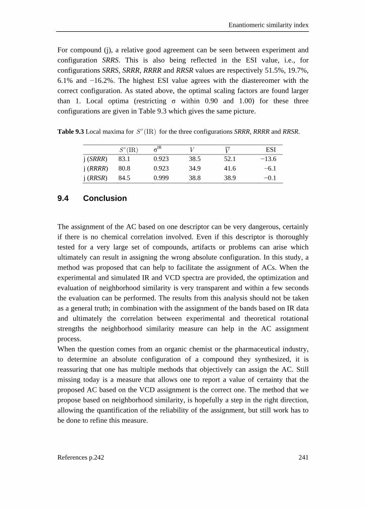
Enantiomeric similarity index
References p.242 241
For compound (j), a relative good agreement can be seen between experiment and configuration SRRS. This is also being reflected in the ESI value, i.e., for configurations SRRS, SRRR, RRRR and RRSR values are respectively 51.5%, 19.7%, 6.1% and −16.2%. The highest ESI value agrees with the diastereomer with the correct configuration. As stated above, the optimal scaling factors are found larger than 1. Local optima (restricting σ within 0.90 and 1.00) for these three configurations are given in Table 9.3 which gives the same picture. Table 9.3 Local maxima for (IR)S σ for the three configurations SRRR, RRRR and RRSR.
(IR)S σ σIR V V ESI j (SRRR) 83.1 0.923 38.5 52.1 −13.6 j (RRRR) 80.8 0.923 34.9 41.6 −6.1 j (RRSR) 84.5 0.999 38.8 38.9 −0.1
9.4 Conclusion
The assignment of the AC based on one descriptor can be very dangerous, certainly if there is no chemical correlation involved. Even if this descriptor is thoroughly tested for a very large set of compounds, artifacts or problems can arise which ultimately can result in assigning the wrong absolute configuration. In this study, a method was proposed that can help to facilitate the assignment of ACs. When the experimental and simulated IR and VCD spectra are provided, the optimization and evaluation of neighborhood similarity is very transparent and within a few seconds the evaluation can be performed. The results from this analysis should not be taken as a general truth; in combination with the assignment of the bands based on IR data and ultimately the correlation between experimental and theoretical rotational strengths the neighborhood similarity measure can help in the AC assignment process. When the question comes from an organic chemist or the pharmaceutical industry, to determine an absolute configuration of a compound they synthesized, it is reassuring that one has multiple methods that objectively can assign the AC. Still missing today is a measure that allows one to report a value of certainty that the proposed AC based on the VCD assignment is the correct one. The method that we propose based on neighborhood similarity, is hopefully a step in the right direction, allowing the quantification of the reliability of the assignment, but still work has to be done to refine this measure.

Chapter 9
242
9.5 Reference list
1. Rouhi, A. M. Chem. Eng. News 2005, 83, 32-33.
2. Flack, H. D.; Bernardinelli, G. Acta. Crystallogr. A 1999, 55, 908-915.
3. Kuppens, T.; Vandyck, K.; Van der Eycken, J.; Herrebout, W.; van der Veken, B. J.; Bultinck, P. Spectrochim. Acta A 2006, In press.
4. Debie, E.; Kuppens, T.; Vandyck, K.; Van der Eycken, J.; van der Veken, B. J.; Herrebout, W.; Bultinck, P. Submitted to Tetrahedron-Asymmetr. 2006
5. Kuppens, T.; Langenaeker, W.; Tollenaere, J. P.; Bultinck, P. J. Phys. Chem. A 2003, 107, 542-553.
6. Kuppens, T.; Vandyck, K.; Van der Eycken, J.; Herrebout, W.; van der Veken, B. J.; Bultinck, P. J. Org. Chem. 2005, 70, 9103-9114.
7. Kruchkov, F. A.; Kuppens, T.; Kolehmainen, E.; Nikiforov, V. A. Organohalogen Compounds 2006, 68. In press.
8. Kuppens, T.; Herrebout, W.; van der Veken, B. J.; Bultinck, P. J. Phys. Chem. A 2006, 100, 10191-10200.
9. Van Daele, G. EP 68544, 1982.
10. Lesage, A.; Bischoff, F. P.; Janssen, C.; Lavreysen, H. WO 2003082350, 2003.
11. Mabire, D.; Venet, M. G.; Coupa, S.; Poncelet, A. P.; Lesage, A. WO 2002028837, 2001.
12. Janssen, P. A. J.; Heeres, J.; Lewi, P. J.; Vlaminck, K.; Ottevaere, P.; Vanparijs, O. WO 2006079642, 2006.
13. Gilkerson, T.; Nash, R.; Van Gestel, J.; Meerpoel, L. WO 2002034752, 2001.
14. Meerpoel, L.; Van Gestel, J.; Van Gerven, F.; Woestenborghs, F.; Marichal, P.; Sipido, V.; Terence, G.; Nash, R.; Corens, D.; Richards, R. D. Bioorg. Med. Chem. Lett. 2005, 15, 3453-3458.
15. Cid-Nunez, J. M.; Megens, A.; Trabanco-Suarez, A. A.; Koukni, M.; Hoornaert, G.; Compernolle, F.; Kozlecki, T.; Mao, H.; Jha, S. C.; Fernandez-Gadea, F. J. WO 2006061392, 2005.

Enantiomeric similarity index
243
16. Mao, H.; Kozlecki, T.; Compernolle, F.; Hoornaert, G. WO 2003048147, 2002.
17. Lang, Y. L.; Medaer, B.; Hoornaert, G.; Brossette, T.; Compernolle, F.; Guillaume, M.; Mao, H.; Kozlecki, T. WO 2003048146, 2002.
18. De Knaep, A.; Moens, L.; Rey, M. WO 9816511, 1997.
19. Van Daele, G.; Bosmans, J. P.; Van Laerhoven, W. US 5674868, 1995.
20. Moehrle, H.; Pycior, M.; Wendisch, D. Pharmazie 1992, 47, 8-10.
21. Kuppens, T.; Herrebout, W.; van der Veken, B. J.; Corens, D.; De Groot, A.; Doyon, A.; Van Lommen, G.; Bultinck, P. Chirality 2006, 18, 609-620.
22. Ashvar, C. S.; Devlin, F. J.; Bak, K. L.; Taylor, P. R.; Stephens, P. J. J. Phys. Chem.-US 1996, 100, 9262-9270.
23. Devlin, F. J.; Stephens, P. J.; Cheeseman, J. R.; Frisch, M. J. J. Phys. Chem. A 1997, 101, 9912-9924.
24. Devlin, F. J.; Finley, J. W.; Stephens, P. J.; Frisch, M. J. J. Phys. Chem.-US 1995, 99, 16883-16902.
25. Stephens, P. J.; Devlin, F. J.; Ashvar, C. S.; Chabalowski, C. F.; Frisch, M. J. Faraday Discuss. 1994, 99, 103-119.
26. Devlin, F. J.; Stephens, P. J.; Cheeseman, J. R.; Frisch, M. J. J. Phys. Chem. A 1997, 101, 6322-6333.
27. He, J. T.; Polavarapu, P. L. J. Chem. Theory Comput. 2005, 1, 506-514.

245
summary and conclusions The primary aim of this research has been the development of a transparent methodology for the measurement and calculation of vibrational circular dichroism (VCD) spectra with the purpose of absolute configuration assignments of chiral molecules in organic synthesis, medicinal chemistry and pharmaceutical industry. The first compound that was examined was hydroxymethyl dihydrodioxinopyridine. This study was the first investigation on the applicability of VCD absolute configuration determination in Belgium. The experimental measurements for this compound were performed by Bruker Optics. In Chapter 5, the basis set dependence was explored, and the outcome was that the 6-31G* is a practicable basis set, but when exact rotational strengths are needed, the cc-pVTZ basis set should be used. The numerical integration grid size was also thoroughly tested, which resulted in the conclusion that the SG1 grid produces very similar spectra compared to the finegrid, with a computational cost reduction of approximately 30%. However, the rotational invariance was lost. No further efforts were taken to investigate the applicability of sparser grids, because additional calculations showed that the rotational invariance could not be preserved. The first measurements that were performed on our own VCD spectrometer are described in Chapter 6. A good agreement was observed between the measured and the simulated spectra for three as-hydrindacene compounds. On the basis of these agreements and after thorough analysis of the spectra, their absolute configuration could be assigned. For hexahydro-as-indacenediol and hydroxy-tetrahydro-as-indacenone the absolute configurations were previously determined by other methods and the absolute configuration of di-epoxy-dihydro-as-indacene was

Summary and conclusions
246
previously unknown. Our absolute configurations based on VCD for the first two compounds were in agreement with the known absolute configurations. In parallel to the previous assignments and following studies, multiple absolute configurations determinations were performed for Johnson & Johnson Pharmaceutical Research and Development (JNJPRD), and are partially listed in the Appendix. Two compounds, studied under the agreement between JNJPRD and Ghent University were published and presented in Chapter 7. The studied compounds, i.e. dichlorophenyl-propanol and dichlorophenyl-propanamine are successive precursors of a potent CCR2 receptor antagonist. The antagonist itself was too large to handle, and would not give as reliable results as the analysis of a smaller precursor molecule. Here, two successive precursors were available in enantiopuric form to assign the absolute configurations of both compounds. This scheme was only possible because no racemization occurs in the synthesis path. The analysis of both compounds, and their corresponding vibrational spectra were a real challenge, because many significant minima were found, which should all be accounted for in order to explain all experimental bands. Ultimately, this resulted in a highly reliable assignment of the absolute configurations of the alcohol and amine derivative, and therefore also absolute configuration of the CCR2 receptor antagonist. For tetrahydrofuran-3-carboxylic acid, a compound that was studied for JNJPRD, the simulated IR and VCD showed no agreement with experiment. Because non-polar solvents are used to eliminate significant solvent interaction with the solute molecules, solvent effects could be ruled out. Also, the applied level of theory was proven to be very reliable. Therefore a different explanation had to be found. As it is known that carboxylic acids in solutions form strong hydrogen-bonded cyclic dimers, the dimers of tetrahydrofuran-3-carboxylic acid were modeled. Simulated vibrational spectra for these dimer geometries showed good agreement with experiment. This result directed the research to the investigation of tetrahydrofuran-2-carboxylic acid. The simulation of spectra for this compound was a real challenge, as neither the dimer nor the monomer structures yielded spectra that were in agreement with experiment. It soon became clear that both monomers and dimers were present in solution. Due to the relative position of the carboxylic acid moiety with respect to the tetrahydrofuran oxygen, intramolecular hydrogen bonding was possible, which stabilized two monomer geometries considerably. Consequently, both monomers

Summary and conclusions
247
and dimers should be taken into account. To obtain usable populations for the monomer and dimer conformations, a semiquantitative model was proposed. This yielded rational values for the populations, which gave spectra in relative good agreement with experiment. Further investigations on this compound were performed by converting the carboxylic acid in a methyl ester. For this compound, i.e., methyl-tetrahydrofuran-2-carboxylate, it was shown that no problems arose with respect to intermolecular associations. Additionally, a systematic study to investigate the performance of the available hybrid functionals in Gaussian03 was performed. B3LYP, B1LYP and B98 proved to be the most reliable for the calculation of rotational strengths for this compound. An important objective of this thesis has been the development of a method allowing transparent and reliable comparison of computed IR and VCD spectra. This started with the introduction of the scaled and normalized overlap integral for experimental and calculated spectra (Chapter 5). However, the main problem with this method is that the inherent differences between experimental and theoretical spectra can not be managed, that is, the local shift of vibrational bands for theory versus experiment. The next step was the introduction of neighborhood comparison, with the aid of cross-correlation functions and a triangular weighting function. A window size of 40 cm−1 was found ideal for the comparison of vibrational spectra. The main problem with this method is the choice of scaling factor. The values in Chapter 6 are achieved, using the maximizing overlap scaling factor. Further development yielded a neighborhood similarity measure that could be optimized by varying the scaling of the theoretical frequencies. Based on this neighborhood similarity measure, the enantiomeric similarity index (ESI) was introduced. This ESI is the difference between the VCD neighborhood similarities for opposite enantiomers for which the scaling factors are obtained by the maximization of the IR neighborhood similarity. The ESI was tested for 21 compounds (Chapter 9) and is shown to be very promising towards the quantification of the reliability of the absolute configuration assignment. Further testing on additional compounds and refinement of the ESI should be performed to confirm these results.

Summary and conclusions
248
Roughly 30 compounds were analyzed for this thesis, and their absolute configurations were successfully assigned. Based on these results one could propose a transparent methodology or guidelines for absolute configuration determination. Prior to presenting such guidelines, it is of utmost importance to stress that these guidelines can merely reflect a rough advice. They should never be considered as dogmatic, and it remains an important task for every user to establish whether or not these guidelines are likely to be acceptable. Failure to establishing this may result in poor determinations of absolute configuration, or even the wrong assignment. As such, the guidelines developed here should be considered only a first step. If any elements appear that suggest the necessity for a closer examination of the application of the guidelines, the VCD user should examine closely the source for any disagreement between theory and experiment. For instance, if bands with wrong sign are predicted, the user should question his/her own computational and experimental strategy and be prepared to go beyond the guidelines and improve e.g. basis sets, functionals, experimental setup, … VCD is not likely to become a black box technique, and experience in quantum chemistry techniques and experimental FTIR is essential. The first step in the process of the AC determination using VCD is the assessment of the behavior of the studied compound in solution. One should have a good understanding of possible intermolecular associations of solute molecules or important solvent/solute interactions. If such interactions are expected, standard gas phase quantum chemical modeling techniques will not suffice and a careful computational and experimental setup should be planned. It may often happen that solvent models in the current state of the art will not sufficiently well describe solvent effects, or could come at a too high computational cost. In such an event, one could study a derivative of the molecule. It was found that for the compounds studied in this thesis containing alcohol and amine functional groups, solvent effects and self-association does not have a large influence on the absolute configuration determination. For carboxylic acids it is adviced to analyse the corresponding methyl ester. The conformational analysis should be performed using a systematic search on a sufficiently high level of theory, preferably B3LYP/6-31G*. For larger molecules this is not practical and it has been shown that the combination of molecular mechanics methods most often yields the same qualitative picture as the DFT search. The minima found during the molecular mechanics conformational search

Summary and conclusions
249
should be optimized further on at least the B3LYP/6-31G* level of theory. A good understanding of the conformational behavior of the studied compound is of the utmost importance as the VCD signature of a molecule is found to be heavily dependent on the conformational properties! The conformational analysis yields a list of all unique stationary points on the potential energy surface (PES). For each unique geometrie one should calculate the dipole and rotational strengths and vibrational frequencies, and one should check if all stationary points that were found are real minima. The B3LYP/6-31G* yields rotational strengths which are often good enough to be compared with experimental VCD intensities, but it has been shown that small differences can occur. The cc-pVTZ basis set yields better rotational strengths, but at a higher computational cost. It has also been shown that in some cases the B3LYP/6-31G* level of theory has problems describing the PES unambiguously. IR and VCD spectra can be simulated based on these calculations, using free energies and Boltzmann statistics to determine the conformational populations. A procedure for the measurement of the experimental VCD spectra on a Bruker PMA37 module can be found in §3.3. For this setup it is extremely important that high quality baselines are acquired by using both enantiomers or the racemic mixture. If these samples are not available, one can use the solvent to approximate the baseline. It goes without saying that the chiral samples should have a high enough enantiomeric excess to perform a reliable assignment. The final step is the comparison of the experimental and simulated spectra. A method which is very tempting, is the superposition of both the theoretical and experimental spectra and on sight comparison. The reliability of this method is not very high, and one should use more elaborate techniques to compare experimental and theoretical spectra. The most reliable technique is to assign the bands in the experimental spectrum based on the fundamental spectrum which was simulated and estimate the area under the experimental bands. The main problem with this method is that it is very time consuming (4–8 hours per compound). The ESI is an alternative to this technique, which gives the same information in a few seconds. Both techniques give the scientist a measure that can be used to quantify the agreement and the reliability of the assignment. The most important step in the simulation of reliable spectra is intermolecular association assessment and the conformational analysis. For all subsequent steps it

Summary and conclusions
250
has been shown that they can be automated in a reliable way and little interaction is required. Using this methodology more than 95% of the compounds studied in this dissertation could be assigned. That VCD has become a powerful method to study absolute configurations and conformational properties of chiral molecules in solution is certain. In Figure 1, an overview of the number of publications per year is presented and it can be seen that more and more scientists are becoming active in the field. Before 1996, most papers where on the fundamentals of FTIR VCD measurements and the theory of VCD intensities. The last 10 years, VCD papers began to appear in experimental and high impact journals e.g., Journal of the American Chemical Society, Journal of Organic Chemistry, Journal of Physical Chemistry, Tetrahedron, etc. More and more experimental scientists and pharmaceutical companies are using this technique combining quantum chemical and experimental expertise.
0
10
20
30
40
50
60
70
80
90
19731974
1975
19761977
19781979
1980
19811982
19831984
19851986
1987
19881989
19901991
1992
19931994
19951996
1997
19981999
20002001
20022003
2004
20052006 (*1)
Figure 1 The number of annual publication of VCD related papers. *1 the cited number for 2006 is incomplete (November 2006). (source: SciFinder Scholar database) For this dissertation much energy was put in the development of a methodology that allows absolute configuration determination. There was absolutely no expertise on this subject in our laboratory. Currently, much experience has been gained, both on the experimentally and theoretically side. New computational standards were introduced on which VCD spectra can be assigned and analyzed even when the conformational behavior of the compounds is complex (see Chapter 7). Also new

Summary and conclusions
251
insights were gained on the VCD of carboxylic acids and intermolecular interaction (see Chapter 8). Based on the results of this dissertation, new and more fundamental questions can be raised. For example, can we perform low temperature measurements, which affect the conformational populations? More interesting is the influence of intermolecular interaction on the vibrational properties of the compounds. In this dissertation it was shown that this is a general problem. There are also indications that the CDCl3 interaction with carbonyl containing compounds has a certain influence on the conformational and vibrational behavior. Further research is needed in this area.
253
samenvatting 1 Inleiding
De biologische activiteit van enantiomeren van chirale geneesmiddelen kan sterk verschillen. Vaak vertoont het ene enantiomeer een farmacologische activiteit, terwijl het andere minder actief of zelfs toxisch kan zijn. Het is bijgevolg uiterst belangrijk de biologische activiteit van specifieke enantiomeren in chirale geneesmiddelen te kennen. De onderzoeksinspanningen hiernaar zijn de laatste jaren sterk toegenomen, vooral gedreven door de snelle ontwikkeling van betere analyse- en scheidingstechnieken en verbeterde synthese routes voor chirale moleculen. Een bedrijf of instelling dat wil overgaan tot klinische testen van een geneesmiddel, of dat zijn medicijn op de markt wil brengen, moet eerst een licentie bekomen bij de regulerende instanties. In de Verenigde Staten kan men zo’n licentie verkrijgen via een New Drug Application (NDA) bij de Food and Drug Administration (FDA). Men moet hiervoor een lijvig rapport samenstellen dat handelt over de actieve component. Voor chirale geneesmiddelen is natuurlijk ook de absolute configuratie van groot belang. Wanneer een farmaceutisch bedrijf zijn intellectuele eigendom op potentiële moleculen wil vrijwaren, dan ook moet de absolute configuratie gekend zijn. De combinatie van de snel groeiende markt van chirale geneesmiddelen en de behoefte aan de kennis van de absolute configuratie van moleculen maakt dat er nood is aan toegankelijke methoden voor de bepaling van absolute configuraties. Eenkristal x-straal diffractie is een zeer belangrijke techniek voor het bepalen van absolute configuraties. Deze techniek is echter niet altijd toepasbaar. Een vereiste is

Samenvatting
254
dat de eenkristallen onderhevig zijn aan anomale verstrooiing. Voor standaard x-straal diffractie experimenten komt dit neer op de aanwezigheid van zware atomen. Een andere methode, elektronisch circulair dichroïsme (ECD), is een vorm van UV/VIS-spectroscopie waarbij links- en rechtsdraaiend circulair gepolariseerd UV/VIS-licht op een verschillende wijze wordt geabsorbeerd door chirale moleculen. Deze methode kan enkel gebruikt worden wanneer de nodige chromofore groepen aanwezig zijn op de moleculen. Andere methoden zijn nucleaire magnetische resonantie (NMR), optische rotatie en stereospecifieke synthese. Een betrekkelijk nieuwe techniek is het vibrationeel circulair dichroïsme (VCD). 2 Vibrationeel circulair dichroïsme Vibrationeel circulair dichroïsme is een techniek, die de structurele specificiteit van infraroodspectroscopie combineert met de stereochemische gevoeligheid van circulair dichroïsme. Het betreft de meting van de differentiële absorptie van circulair gepolariseerde infrarood straling. Deze methode heeft als voordeel dat de metingen op nagenoeg exact dezelfde manier kunnen gebeuren als infrarood experimenten, en dat ze dus relatief weinig eisen stellen aan de moleculen. Zo kunnen de VCD metingen ook in oplossingen gebeuren. VCD is een zeer interessante techniek aangezien vibrationele transities in chirale moleculen de oorsprong zijn van de VCD-intensiteiten. Gewone IR-spectra bevatten echter geen stereochemische informatie aangezien IR-spectra van enantiomeren identiek zijn; de VCD-spectra zijn echter spiegelbeelden van elkaar (gespiegeld over de frequentie-as). Omdat VCD een differentiële spectroscopische techniek is, kunnen deze intensiteiten dus ook negatief zijn, waarbij de banden zijn gecentreerd op de vibrationele frequenties. Experimentele spectra werden voor het eerst gerapporteerd in 1973 door Holzwarth et al. De implementatie van Fourier-getransformeerde VCD door Nafie et al. in 1979 en verdere ontwikkelingen van de instrumentatie, maakt dat we tegenwoordig hoge kwaliteit VCD-spectra kunnen opmeten voor de meeste chirale moleculen in oplossing. De interpretatie en evaluatie van experimentele VCD-spectra is niet voor de hand liggend. In vergelijking met de klassieke infrarood spectroscopie komt er bij de verklaring van VCD-spectra nog een extra dimensie bij, met name het teken van de
Samenvatting
255
VCD-intensiteiten. Deze zijn niet eenvoudig interpreteerbaar. Voor een bepaald enantiomeer zijn sommige banden positief en andere negatief zonder dat dit gemakkelijk kan worden gerationaliseerd. Het is in deze context dat de kwantumchemie een grote ondersteunende rol speelt. In het midden van de jaren tachtig werd een theorie ontwikkeld die toelaat om ab initio VCD-intensiteiten te bereken. Deze theorie werd dan ook snel geïmplementeerd, gebruikmakend van Hartree-Fock theorie. De resultaten hiervan waren echter niet accuraat genoeg om vergelijking met experimentele resultaten toe te laten. Het gebruik van Møller-Plesset perturbatie theorie leverde wel goede resultaten, maar door de computationele vereisten was deze methode niet echt haalbaar. De ontwikkeling van density functional theory (DFT) en de introductie van hybride functionalen in het begin van de jaren negentig, betekende een doorbraak voor de berekening van VCD-intensiteiten. Met behulp van DFT- en hybride-functionalen kunnen theoretische spectra van goede kwaliteit bekomen worden, in overeenstemming met experimentele waarnemingen en met rationele computationele kost. 3 Doelstelling van dit onderzoekswerk De implementatie van de theorie voor het berekenen van VCD-intensiteiten op DFT niveau in het commercieel kwantumchemisch rekenpakket Gaussian en de commercialisering van VCD-spectrometers heeft ertoe geleid dat absolute configuratie bepaling d.m.v. VCD meer toegankelijk is geworden. Maar een grote doorbraak zal er enkel komen als ook de methode toegankelijker wordt gemaakt. Momenteel is de drempel voor het uitvoeren van kwantumchemische berekeningen nog te hoog voor niet theoretisch georiënteerde wetenschappers. Het doel van deze thesis is de kracht van deze techniek te bevestigen en een methodologie te ontwikkelen die toelaat om op een transparante en toegankelijke wijze VCD-spectra te berekenen voor de absolute configuratie bepaling van chirale moleculen. Deze doelstelling kan als volgt worden onderverdeeld:
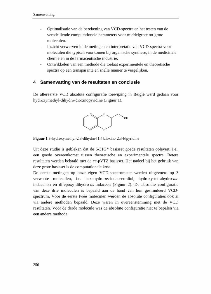
Samenvatting
256
- Optimalisatie van de berekening van VCD-spectra en het testen van de verschillende computationele parameters voor middelgrote tot grote moleculen.
- Inzicht verwerven in de metingen en interpretatie van VCD-spectra voor moleculen die typisch voorkomen bij organische synthese, in de medicinale chemie en in de farmaceutische industrie.
- Ontwikkelen van een methode die toelaat experimentele en theoretische spectra op een transparante en snelle manier te vergelijken.
4 Samenvatting van de resultaten en conclusie De allereerste VCD absolute configuratie toewijzing in België werd gedaan voor hydroxymethyl-dihydro-dioxinopyridine (Figuur 1).
N
O
OOH
Figuur 1 3-hydroxymethyl-2,3-dihydro-[1,4]dioxino[2,3-b]pyridine Uit deze studie is gebleken dat de 6-31G* basisset goede resultaten oplevert, i.e., een goede overeenkomst tussen theoretische en experimentele spectra. Betere resultaten werden behaald met de cc-pVTZ basisset. Het nadeel bij het gebruik van deze grote basisset is de computationele kost. De eerste metingen op onze eigen VCD-spectrometer werden uitgevoerd op 3 verwante moleculen, i.e. hexahydro-as-indaceen-diol, hydroxy-tetrahydro-as-indacenon en di-epoxy-dihydro-as-indaceen (Figuur 2). De absolute configuratie van deze drie moleculen is bepaald aan de hand van hun gesimuleerd VCD-spectrum. Voor de eerste twee moleculen werden de absolute configuraties ook al via andere methoden bepaald. Deze waren in overeenstemming met de VCD resultaten. Voor de derde molecule was de absolute configuratie niet te bepalen via een andere methode.

Samenvatting
257
HOOH HOO OO
Figuur 2 1,2,3,6,7,8-hexahydro-as-indacen-1,8-diol, 8-hydroxy-3,6,7,8-tetrahydro-2H-as-indacen-1-on en 1,2,7,8-di-epoxy-3,6-dihydro-as-indaceen In deze thesis werden eveneens absolute configuratie bepalingen gedaan voor 21 moleculen van Johnson & Johnson Pharmaceutical R&D (JNJPRD). Twee moleculen van deze lijst werden gepubliceerd, i.e. dichlorophenyl-propanol en dichlorophenyl-propaanamine (Figuur 3). Beide zijn opeenvolgende precursoren van een krachtige CCR2 receptor antagonist. Aangezien de moleculaire structuur van de antagonist te groot was om te behandelen, werden de absolute configuraties van de kleinere precursoren bepaald. Dit was mogelijk omdat er in de verdere synthese stappen geen racemisatie optreedt. De simulatie van de spectra werd gedaan op B3LYP/cc-pVTZ niveau en een goede overeenkomst met de experimentele spectra werd gevonden. Dit resulteerde in een betrouwbare toewijzing van de absolute configuratie van de twee precursoren en de eigenlijke CCR2 receptor antagonist.
Cl
ClN
O
OHS
N
O
O
Cl
Cl
OHCl
NH2
Cl
Figuur 3 Dichlorophenyl-propanol, dichlorophenyl-propaanamine en de CCR2 receptor antagonist. Bij het opnemen van de experimentele spectra worden de te bestuderen moleculen meestal opgelost in apolaire solventen om een mogelijke interactie tussen solvent en opgelost product te vermijden. Voor tetrahydrofuran-3-carboxylzuur stelden we echter vast dat de gesimuleerde IR- en VCD-spectra geen overeenkomst vertoonden met de experimentele spectra. Dit verschil was blijkbaar te wijten aan zelfassociatie van het carbonzuur in de apolaire oplossing. Wanneer theoretische spectra werden gesimuleerd van gemodelleerde dimeer-structuren (Figuur 4), werd wel overeenkomst met het experiment gevonden.

Samenvatting
258
O
O
O H
O
O
OH
Figuur 4 Cyclische dimeer-structuur van tetrahydrofuran-3-carboxylzuur Deze bevinding leidde het onderzoek naar een studie rond tetrahydrofuran-2-carbonzuur (Figuur 5). De simulatie van de VCD- en IR-spectra voor deze molecule was niet voor de hand liggend, omdat in dit geval noch de spectra voor het gesimuleerde monomeer, noch de dimeer-spectra overeen kwamen met de experimentele spectra. De conformationele eigenschappen van het 2-isomeer waren immers van die aard dat er stabiliserende intra-moleculaire waterstofbruggen gevormd konden worden in het monomeer. In oplossing was er dus zowel monomeer als dimeer aanwezig. Er werd een semi-kwantitatief model opgesteld om bruikbare conformationele populaties van het monomeer en dimeer te vinden. Op basis van dit model werden spectra gesimuleerd die een goede overeenkomst vertoonden met de experimentele spectra.
O
O
O
H
O
O
O
Figuur 5 Tetrahydrofuran-2-carbonzuur en het methyl-tetrahydrofuran-2-carboxylaat In navolging van dit onderzoek werd er ook een studie uitgevoerd op het methylester van het 2-isomeer, i.e. methyl-tetrahydrofuran-2-carboxylaat (Figuur 5). Hieruit bleek dat er voor het methylester geen hinderlijke intermoleculaire associatie aanwezig was. Verder werd er ook een systematische studie uitgevoerd op verschillende hybride functionalen waaruit volgde dat de B3LYP, B1LYP en B98 functionalen de beste resultaten opleverden voor het simuleren van VCD-spectra. In dit onderzoek werd ook een transparante methode voor het vergelijken van experimentele en theoretische spectra uitgewerkt.

Samenvatting
259
De aanvankelijk voorgestelde maat voor similariteit van spectra was een genormaliseerde overlap integraal. Het grote probleem bij dergelijk type van vergelijkingen is het inherent verschil tussen experimentele en theoretische vibrationele spectra. De berekende vibrationele frequenties worden systematisch overschat. Hiervoor kan gedeeltelijk worden gecompenseerd via lineaire schaling, maar zelfs dan worden er nog steeds locale verschuivingen waargenomen tussen corresponderende experimentele en theoretische banden. Om die reden werd een nieuwe maat voor similariteit ingevoerd die rekening houdt met de omgeving van de beschouwde banden door gebruik te maken van een genormaliseerde kruiscorrelatiefunctie en een driehoekige gewichtsfunctie. Deze omgevings-similariteitsmaat is natuurlijk afhankelijk van de frequentie schalings-factor. Verdere ontwikkeling stelde ons in staat om de omgevings-similariteit te optimaliseren door de schalingsfactor te variëren. Op basis van deze omgevings-similariteitsmaat hebben we de enantiomerische similariteitsindex (ESI) geïntroduceerd. De ESI is het verschil tussen de VCD omgevings-similariteiten (t.o.v. het experimentele VCD) van beide enantiomeren. Deze ESI is getest voor 21 moleculen en de resultaten geven aan dat dit een veelbelovende maat is voor het kwantificeren van de betrouwbaarheid van een absolute configuratie bepaling. Gedurende dit doctoraal onderzoek werden een dertigtal moleculen geanalyseerd, en hun absolute configuraties werden met succes toegewezen. Gebaseerd op de expertise die aldus werd opgebouwd en in dit werk naar voor komt, zou men een transparante methodologie en een set van richtlijnen voor absolute configuratie bepaling kunnen voorstellen. Deze richtlijnen zijn enkel bedoeld als leidraad en het moet benadrukt worden dat het aan de VCD-gebruiker is om in te schatten of deze richtlijnen voldoen voor het specifieke probleem. Het kan zijn dat er bij het volgen van deze richtlijnen elementen opduiken die wijzen op het feit dat er een verdergaande analyse nodig is. Zo kunnen er bijvoorbeeld banden worden voorspeld met een verkeerd teken. Het is aan de VCD-gebruiker om de relevantie van het probleem in te schatten en eventueel de experimentele en/of reken-strategie te herzien. Het is hoe dan ook noodzakelijk om een grondige expertise in de gebruikte kwantum chemische en experimentele FTIR-technieken te hebben. De eerste stap in het proces van een absolute configuratie bepaling op basis van VCD is een grondige analyse van het gedrag van de molecule in oplossing. Het is zeer belangrijk dat men een goed zicht heeft op het intermoleculair associatiegedrag
Samenvatting
260
van de opgeloste molecule onderling of van opgeloste molecule en solvent. Als dergelijke interacties te verwachten zijn, voldoen standaard kwantum chemische gas fase berekeningen vaak niet, en is een uitgebreidere modellering nodig, alsook verdere experimentele metingen. Men kan trachten het associatie gedrag te modelleren waarbij verscheidene modellen kunnen aangewend worden. Als blijkt dat deze modellen niet toereikend zijn of een te hoge rekentijd met zich meebrengen dan kan er eventueel worden overgegaan tot het derivatiseren van de molecule. Voor de alcoholen en amines bestudeerd in dit werk zijn de solvent en zelfassociatie effecten niet significant gebleken voor de toepassing van absolute configuratie bepaling. Voor carbonzuren is het aangeraden om het corresponderende methylester te bestuderen. De conformationele analyse zou op een zo hoog mogelijk niveau moeten gebeuren, bij voorkeur B3LYP/6-31G* niveau. Voor grotere moleculen is het praktischer om een combinatie van moleculair mechanische methoden te gebruiken. Een dergelijke aanpak geeft veelal hetzelfde conformationele beeld. De minima die gevonden worden gedurende een moleculair mechanische conformationele zoektocht zouden vervolgens geoptimaliseerd moeten worden op het B3LYP/6-31G* niveau. Gezien de conformationele gevoeligheid van VCD is een goed begrip van het conformationele gedrag van de bestudeerde molecule uiterst belangrijk. Een conformationele analyse levert een lijst op met unieke stationaire punten op het potentiaal oppervlak. Voor alle unieke geometrieën moet men de dipool en rotationele sterktes berekenen samen met de vibrationele frequenties. Men moet zich er ook van vergewissen dat alle stationaire punten echte minima zijn. Het B3LYP/6-31G* krachtveld levert rotationele sterktes op die vergelijkbaar zijn met experimentele VCD-intensiteiten. In sommige gevallen worden er kleine verschillen geobserveerd. Het is ook aangetoond dat het B3LYP/6-31G* soms problemen heeft om het potentiaaloppervlak ondubbelzinnig te beschrijven. De cc-pVTZ basisset is een beter keuze, maar brengt dan ook langere rekentijden met zich mee. IR- en VCD-spectra kunnen gesimuleerd worden op basis van deze berekening, gebruikmakend van vrije energieën en Boltzmann-statistiek om de conformationele populaties te berekenen. Voor de meting van VCD verwijzen we naar §3.3 waar uitgebreid staat beschreven hoe men betrouwbare spectra kan bekomen op de PMA37 VCD-module van Bruker. Voor een dergelijke configuratie is het zeer belangrijk om een goede basislijn te bekomen gebruik makend van beide enantiomeren of het racemisch mengsel.

Samenvatting
261
Wanneer deze niet voorhanden zijn kan men de basislijn benaderend bepalen met behulp van het solvent. De chirale samples moeten natuurlijk een voldoende hoge enantiomere overmaat hebben om een betrouwbare toewijzing te kunnen doen. De finale stap is de vergelijking van experimentele en gesimuleerde spectra. Een voor de hand liggende maar onbetrouwbare methode is het op elkaar leggen van het experimentele en theoretische spectrum. De meest betrouwbare methode is het toewijzen van de experimentele banden op basis van het theoretische spectrum, en het bepalen van de oppervlakte onder de experimentele banden. Het probleem met deze methode is het arbeidsintensieve karakter, i.e., 4 tot 8 uur per molecule. De door ons ontwikkelde ESI is een alternatieve methode die dezelfde informatie geeft in enkele seconden. Beide technieken geven de gebruiker een maat van overeenkomst en betrouwbaarheid van de toewijzing. De belangrijkste stap in de simulatie van VCD-spectra is de inschatting van mogelijke intermoleculaire associaties en de conformationele analyse. De stappen die hierop volgen werden allemaal geautomatiseerd waardoor de analyse niet veel interactie meer behoeft. Meer dan 95% van de moleculen bestudeerd voor deze thesis konden worden toegewezen gebruikmakend van de hierboven beschreven methodologie. Het is duidelijk dat VCD een krachtige techniek is geworden om de absolute configuratie en conformationele eigenschappen van chirale moleculen in oplossingen te analyseren. Figuur 6 geeft de evolutie van het aantal VCD gerelateerde publicaties per jaar en hieruit blijkt dat de wetenschappelijke reikwijdte steeds groter wordt. De publicaties daterend vóór 1996 handelen voornamelijk over de theorie van VCD-intensiteiten en FTIR VCD. Gedurende de laatste tien jaar is de frequentie van VCD publicaties sterk toegenomen in tijdschriften met een hoge impact factor en experimentele tijdschriften zoals bijvoorbeeld Journal of the American Chemical Society, Journal of Organic Chemistry, Journal of Physical Chemistry, Tetrahedron, enz. De interesse vanuit de experimentele hoek en de farmaceutische industrie neemt sterk toe, waarbij de combinatie van de experimentele en kwantum chemische expertise goed tot uiting komt.

Samenvatting
262
0
10
20
30
40
50
60
70
80
90
19731974
1975
19761977
19781979
1980
19811982
19831984
19851986
1987
19881989
19901991
1992
19931994
19951996
1997
19981999
20002001
20022003
2004
20052006 (*1)
Figuur 6 Het jaarlijkse aantal VCD gerelateerde publicaties. Het geciteerde getal voor 2006 is onvolledig (november 2006). (bron: SciFinder Scholar database) Gedurende dit werk werd veel aandacht en energie geïnvesteerd in de ontwikkeling van een methodologie voor absolute configuratie bepalingen. Immers, deze methode werd de onderzoeksgroep binnengehaald met dit doctoraatsonderzoek en state-of-the art expertise werd opgebouwd met als resultaat een aanzienlijk aantal publicaties in hoog gewaardeerde wetenschappelijke tijdschriften. Momenteel is zowel de experimentele als de theoretische expertise aanwezig en kunnen toekenningen op een relatief transparante wijze worden voltooid. Met dit werk werden ook nieuwe theoretische standaarden geïntroduceerd op basis waarvan de VCD-spectra kunnen worden toegekend en geanalyseerd, zelfs wanneer het conformationeel gedrag van de moleculen bijzonder complex is (zie Hoofdstuk 7). Er werden bovendien ook bijkomende inzichten verworven in de VCD analyse van carbonzuren en de optredende intermoleculaire interacties (zie Hoofdstuk 8). Als resultaat van de kennisopbouw bij deze thesis, kunnen nieuwe fundamentele vragen gesteld worden. Zo is er bijvoorbeeld de bemerking of we lage temperatuur VCD analyses kunnen uitvoeren en welke invloed dit zal hebben op de conformationele populaties. Zoals ook naar voor komt in deze thesis is een systematische studie naar de invloed van intermoleculaire interacties op de vibrationele eigenschappen van moleculen van bijzondere interesse. Er zijn aanwijzingen dat de CDCl3 interactie met de carbonyl groepen van een molecule een significante invloed hebben op de conformationele en vibrationele eigenschappen van de verbinding. Verder onderzoek in deze richting is nuttig en uiterst interessant.
References p.273 263
Appendix
unreported AC assignments Background
In the last quarter of 2003, an agreement was closed between Ghent University and Johnson & Johnson Pharmaceutical Research and Development (JNJPRD) in which was declared that Ghent Quantum Chemistry Group would perform the calculations and the actual assignments for AC determination based on VCD. These assignments involve drugs discovery compounds. Until now, a total of 21 compounds were processed for JNJPRD. Due to intellectual property restrictions not all structures can be published in this dissertation. All successful assignments, for which the intellectual property rights have been secured, are given briefly in this appendix. Experimental and simulated spectra are presented together with additional information on measurement conditions and the structure, name and internal JNJ code. The calculations were all performed using the B3LYP functional and the 6-31G* basis set. For some compounds also cc-pVTZ spectra were calculated. The figures are arranged in the following fashion,
(B3LYP/cc-pVTZ) B3LYP/6-31G*
Experimental

Appendix
264
The 6-31G* and cc-pVTZ frequencies are respectively scaled with a factor 0.967 and 0.980. The last assignment in this chapter is an assignment performed for Prof. Dr. V. Nikiforov from the St. Petersburg State University. For this compound the absolute configuration determination was not possible nor with XRD nor with NMR methods.

Unreported AC assignments
References p.273 265
HNN
O
N*
3,3-Dimethyl-hexahydro-imidazo[1,5-α]pyrazin-1-one JNJ6202391 JNJ16927053
Origin – JNJPRD ref 1 Measurements – Performed by JNJPRD - Enantiomeric pure sample Modeled configuration – S Number of significant conformations – 2 Spectra – No CO stretch spectra due to high absorbance in this
region.
1500 1400 1300 1200 1100 1000
0.0
0.2
0.4
0.6
0
50
100
150
200
250
300
350
A
ε
1500 1400 1300 1200 1100 1000
-6.0x10⁻⁵
-4.0x10⁻⁵
-2.0x10⁻⁵
0.0
2.0x10⁻⁵
4.0x10⁻⁵
6.0x10⁻⁵
-0.02
-0.01
0.00
0.01
0.02
0.03
Δ ε
Δ A
Figure A1

Appendix
266
OO
F
*
1-(6-fluorochroman-2-yl)ethanone JNJ17341727
Origin – JNJPRD refs 2,3 Measurements – Performed by JNJPRD - Both enantiomers in CD2Cl2 Modeled configuration – S Number of significant conformations – 2 Spectra – Half difference
1800 1700 1600 1500 1400 1300 1200 1100 1000
0.0
0.5
1.0
1.50
100
200
300
400
500
600
700
ε
A
1800 1700 1600 1500 1400 1300 1200 1100 1000-0.10
-0.08
-0.06
-0.04
-0.02
0.00
0.02
0.04
0.06
0.08
0.10
-0.01
0.00
0.01
0.02
Δ ε
Δ A
Figure A2

Unreported AC assignments
References p.273 267
NO2
NN
S
*
2,3,5,6-tetrahydro-6-(3-nitrophenyl)-imidazo[2,1b]thiazole
JNJ17139652 JNJ17321343
Origin – JNJPRD ref 4 Measurements – Performed by JNJPRD - Both enantiomers in CDCl3 Modeled configuration – R Number of significant conformations – 4 Spectra – Half difference
1700 1600 1500 1400 1300 1200 1100 1000
0.0
0.5
1.0
0
200
400
600
800
ε
A
1700 1600 1500 1400 1300 1200 1100 1000
-0.1
0.0
0.1
0.2
-0.04
-0.02
0.00
0.02
0.04
Δ ε
Δ A
Figure A3

Appendix
268
N
NHCl
*
1-Chloro-8-ethyl-5,6-dihydro-4-phenyl-4H-pyrrolo[1,2-a][1,4]benzodiazepine
JNJ16709368 JNJ16709407 JNJ16992508
Origin – JNJPRD refs 5,6 Measurements – Performed by JNJPRD - Both enantiomers in CD2Cl2 Modeled configuration – S Number of significant conformations – 7 Spectra – Half difference
1600 1500 1400 1300 1200 1100 1000
0
1
2
3 0
100
200
300
400
ε
A
1600 1500 1400 1300 1200 1100 1000-2.0x10⁻⁴
-1.0x10⁻⁴
0.0
1.0x10⁻⁴ -0.03
-0.02
-0.01
0.00
0.01
0.02
0.03
Δ ε
Δ A
Figure A4
VCD AC determination was published in Meerpoel, L.; Van Gestel, J.; Van Gerven, F.; Woestenborghs, F.; Marichal, P.; Sipido, V.; Terence, G.; Nash, R.; Corens, D.; Richards, R. D. Pyrrolo[1,2-a][1,4]benzodiazepine: A novel class of non-azole anti-dermatophyte anti-fungal agents. Bioorg. Med. Chem. Lett. 2005, 15, 3453-3458.
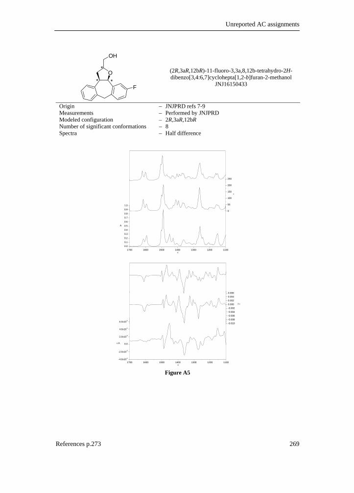
Unreported AC assignments
References p.273 269
O
OH
F
*
**
(2R,3aR,12bR)-11-fluoro-3,3a,8,12b-tetrahydro-2H-dibenzo[3,4:6,7]cyclohepta[1,2-b]furan-2-methanol
JNJ16150433
Origin – JNJPRD refs 7-9 Measurements – Performed by JNJPRD Modeled configuration – 2R,3aR,12bR Number of significant conformations – 8 Spectra – Half difference
1700 1600 1500 1400 1300 1200 11000.0
0.1
0.2
0.3
0.4
0.5
0.6
0.7
0.8
0.9
1.0
ν
0
50
100
150
200
250
ε
A
1700 1600 1500 1400 1300 1200 1100-4.0x10⁻⁵
-2.0x10⁻⁵
0.0
2.0x10⁻⁵
4.0x10⁻⁵
6.0x10⁻⁵
ν
-0.010-0.008-0.006-0.004-0.0020.0000.0020.0040.006
Δ ε
Δ A
Figure A5

Appendix
270
HN
OCH3
NH2**
3-methoxypiperidin-4-amine JNJ16502655 JNJ16159039
Origin – JNJPRD refs 10,11 Measurements – Performed by JNJPRD Modeled configuration – 3R,4S Number of significant conformations – 13
1500 1400 1300 1200 1100 10000.0
0.2
0.4
0.6
0.8
1.0
ν
0
50
100
150
200
250
300
350
ε
A
1500 1400 1300 1200 1100 1000-1.0x10⁻⁴
-8.0x10⁻⁵
-6.0x10⁻⁵
-4.0x10⁻⁵
-2.0x10⁻⁵
0.0
2.0x10⁻⁵
4.0x10⁻⁵
-0.020
-0.015
-0.010
-0.005
0.000
0.005
0.010
Δ ε
Δ A
Figure A6
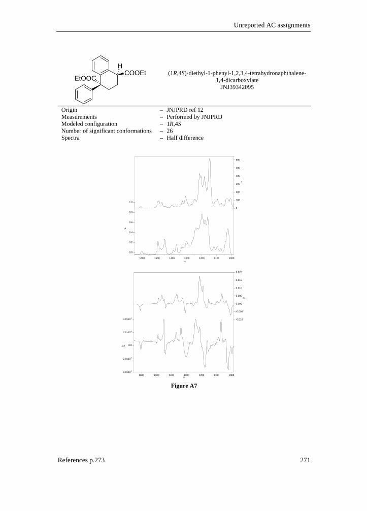
Unreported AC assignments
References p.273 271
EtOOCCOOEt
H
(1R,4S)-diethyl-1-phenyl-1,2,3,4-tetrahydronaphthalene-1,4-dicarboxylate
JNJ39342095
Origin – JNJPRD ref 12 Measurements – Performed by JNJPRD Modeled configuration – 1R,4S Number of significant conformations – 26 Spectra – Half difference
1600 1500 1400 1300 1200 1100 1000
0.0
0.2
0.4
0.6
0.8
1.0
ν
0
100
200
300
400
500
600
ε
A
1600 1500 1400 1300 1200 1100 1000-4.0x10⁻⁵
-2.0x10⁻⁵
0.0
2.0x10⁻⁵
4.0x10⁻⁵
ν
-0.010
-0.005
0.000
0.005
0.010
0.015
0.020
Δ ε
Δ A
Figure A7

Appendix
272
CH2ClCl2HC
CHCl2
ClCl
Cl
Cl
Cl
**
*
* *
*
(1R,3S,4S,5S,6S,7R)-2,2,3-exo,5-endo,6-exo,8,9,9,10,10-decachlorobornane
Origin – Prof. Dr. V. Nikiforov – St. Petersburg State University ref 13
Measurements – Racemic mixture and enantiomeric pure samples at 0.17M in CS2. Measured in KBr cell with 105 µm spacers.
Modeled configuration – 1R,3S,4S,5S,6S,7R Number of significant conformations – 1 Spectra – Racemic baseline corrected.
1400 1300 1200 1100 1000 900 800 7000
50
100
150
200
250
300
350
ε
0
50
100
150
200
ε
1400 1300 1200 1100 1000 900 800-0.03
-0.02
-0.01
0.00
0.01
0.02
-0.03
-0.02
-0.01
0.00
0.01
0.02
0.03
Δ ε
Δ ε
Figure A8
Based on the synthesis, only two enantiomers are possible. The absolute configuration could not be determined by XRD or NMR. AC determination was presented at DIOXIN2006: Structure elucidation of poly-chloroterpenes obtained from optically active pinenes13

Unreported AC assignments
273
Reference list
1. Van Daele, G. EP 68544, 1982.
2. Lesage, A.; Bischoff, F. P.; Janssen, C.; Lavreysen, H. WO 2003082350, 2003.
3. Mabire, D.; Venet, M. G.; Coupa, S.; Poncelet, A. P.; Lesage, WO 2002028837, 2001.
4. Janssen, P. A. J.; Heeres, J.; Lewi, P. J.; Vlaminck, K.; Ottevaere, P.; Vanparijs, O. WO 2006079642, 2006.
5. Gilkerson, T.; Nash, R.; Van Gestel, J.; Meerpoel, L. WO 2002034752, 2001.
6. Meerpoel, L.; Van Gestel, J.; Van Gerven, F.; Woestenborghs, F.; Marichal, P.; Sipido, V.; Terence, G.; Nash, R.; Corens, D.; Richards, R. D. Bioorg. Med. Chem. Lett. 2005, 15, 3453-3458.
7. Cid-Nunez, J. M.; Megens, A.; Trabanco-Suarez, A. A.; Koukni, M.; Hoornaert, G.; Compernolle, F.; Kozlecki, T.; Mao, H.; Jha, S. C.; Fernandez-Gadea, F. J. WO 2006061392, 2005.
8. Mao, H.; Kozlecki, T.; Compernolle, F.; Hoornaert, G. WO 2003048147, 2002.
9. Lang, Y. L.; Medaer, B.; Hoornaert, G.; Brossette, T.; Compernolle, F.; Guillaume, M.; Mao, H.; Kozlecki, T. WO 2003048146, 2002.
10. De Knaep, A.; Moens, L.; Rey, M. WO 9816511, 1997.
11. Van Daele, G.; Bosmans, J. P.; Van Laerhoven, W. US 5674868, 1995.
12. Moehrle, H.; Pycior, M.; Wendisch, D. Pharmazie 1992, 47, 8-10.
13. Kruchkov, F. A.; Kuppens, T.; Kolehmainen, E.; Nikiforov, V. A. Organohalogen Compounds 2006, 68, In press.
acknowledgements
De eekhoorn liep naar het smalle strand van zand en kiezelstenen dat zich uitstrekte langs de rivier. Hij was van plan om daar te gaan nadenken. Hij wist nog niet waarover, maar dat was altijd zo als hij wilde gaan nadenken. Als hij wel had geweten waarover hij wilde nadenken was hij thuis gebleven en had hij daar meteen nagedacht over datgene waarover hij wilde nadenken.
– Toon Tellegen, Er ging geen dag voorbij Ik dank mijn promotor Prof. Dr. Patrick Bultinck, omdat hij me de kans heeft gegeven dit doctoraatsonderzoek aan te vangen en dat ik nu met succes kan afronden. Bedankt voor het vertrouwen en de hand boven mijn hoofd. Het was in de eerste jaren echter niet gemakkelijk om een weg te vinden in de wereld van het VCD onderzoek. In die periode kon ik binnen de vakgroep ook rekenen op de steun van Prof. Dr. André Goeminne. Aan de Universiteit Antwerpen waren het vooral Prof. Dr. Wouter Herrebout en Prof. Dr. Ben van der Veken die me met enthousiasme in dit werk hebben gesteund en ik wil hen dan ook graag bedanken voor hun gastvrijheid en de ondersteuning die ze vanuit hun perspectief gaven aan mijn werk. De samenwerking met het organische synthese labo van Prof. Dr. Johan Van der Eycken was eveneens heel vruchtbaar. Meerdere interessante resultaten werden samen met Dr. Koen Vandyck bekomen en tot in de puntjes uitgewerkt. Koen ben ik dan ook heel dankbaar. De inspiratie voor de opzet van dit onderzoeksproject kwam van Dr. Wilfried Langenaeker en Prof. Dr. Jan Tollenaere, toen werkzaam bij Janssen Pharmaceutica, Beerse. Aan de vorm en samenstelling is in de loop van de jaren misschien wel het één en het ander veranderd, maar de samenwerking met Johnson & Johnson Pharmaceutical Research and Development in Beerse is gebleven. Momenteel is Dr. David Corens daar de drijvende kracht achter de VCD absolute configuratie bepalingen en samen met hem heb ik een groot aantal toewijzingen uitgevoerd. Tenslotte ben ik ook Dr. Guy Van Lommen dankbaar voor de vlotte samenwerking.

I would like to thank Prof. Ramon Carbó-Dorca for his kindness and his help on diverse problems. I'm also grateful for the many constructive comments and remarks I have received from all the anonymous referees during the years. They have improved the quality of this work considerably and have stretched it towards the highest possible level. Dank aan de collega’s in Gent en Antwerpen! Ik wil ook al mijn vrienden danken voor hun steun. In het bijzonder: Raju, zelfs aan de andere kant van de wereld ben je nog steeds een bron van inspiratie en motivatie. Sabina, wat was het leuk om naar jouw verhaaltjes te luisteren. Ik heb het zelfs niet kunnen laten om hierboven een filosofische noot van Eek te plaatsten. Bedankt ook voor je steeds luisterend oor! Lieve, merci voor de zalige ontspannende dineetjes en de vele gesprekken over de meest uiteenlopende onderwerpen. Driesken, ge hebt een jaar in Gent gewoond en het was leuk om zo kort bij huis familie te hebben. Spijtig dat ik het afgelopen jaar zo wreed druk heb gehad. Christy, bedankt voor je steun en je engelengeduld. Mijn ouders en mijn broer Bart wil ik graag bedanken voor de jarenlange en onvoorwaardelijke steun.
Tom Kuppens, december 2006
P.S. Ik zal een marathon lopen binnen dit en twee jaar. (Zo, nu kan ik er niet meer onderuit komen met een flauw excuus)
P.P.S. Ik vergeet nog iemand, nl. mijn gevederde vriend QTux, die mij gezelschap hield bij het creëren van mijn computer cluster (“Ghent quantum cluster” :). Hier staat niets van vermeld in mijn doctoraat. Het is echter praktisch onmogelijk om zware berekeningen uit te voeren zonder een serieuze computer infrastructuur. Ons heterogene en steeds groter wordende computerpark heb ik dan ook op een bepaald moment gebald in een cluster waarbij je op 30 computers tegelijk kan rekenen (en makkelijk uitbreidbaar), ook al lijkt het dat je er maar één aan het bedienen bent. Dit is naast mijn doctoraat waarschijnlijk mijn belangrijkste bijdrage aan de onderzoeksgroep.

TOM KUPPENS
development of methodology to assign absolute
configurations using vibrational circular dichroism
Supplementary Material
promotor: Prof. Dr. P. Bultinck, Ghent University
co-promotor: Prof. Dr. W. Herrebout, University of Antwerp
Dissertation for the degree of Doctor in Sciences: Chemistry – December 2006 Ghent University, Faculty of Sciences Department of Inorganic and Physical Chemistry

S1
CHAPTER 5 _______________________________________________________________ 3
Table S5.1 _____________________________________________________________________ 4
Table S5.2 _____________________________________________________________________ 4
CHAPTER 6 _______________________________________________________________ 5
Table S6.1 _____________________________________________________________________ 6
Table S6.2 _____________________________________________________________________ 7
Table S6.3 _____________________________________________________________________ 8
Table S6.4 _____________________________________________________________________ 9
Table S6.5 ____________________________________________________________________ 10
Table S6.6 ____________________________________________________________________ 11
Table S6.7 ____________________________________________________________________ 12
Figure S6.1 ___________________________________________________________________ 13
Figure S6.2 ___________________________________________________________________ 14
Figure S6.3 ___________________________________________________________________ 15
Figure S6.4 ___________________________________________________________________ 16
Figure S6.5 ___________________________________________________________________ 17
Figure S6.6 ___________________________________________________________________ 18
Figure S6.7 ___________________________________________________________________ 19
Figure S6.8 ___________________________________________________________________ 20
General experimental methods ____________________________________________________ 21
CHAPTER 7 ______________________________________________________________ 25
Table S7.1 ____________________________________________________________________ 26
Table S7.2 ____________________________________________________________________ 29
Figure S7.1 ___________________________________________________________________ 33
Figure S7.2 ___________________________________________________________________ 34

S2
CHAPTER 8 ______________________________________________________________ 35
Table S8.1 ____________________________________________________________________ 36
Table S8.2 ____________________________________________________________________ 37
Table S8.3 ____________________________________________________________________ 38
Table S8.4 ____________________________________________________________________ 39
Table S8.5 ____________________________________________________________________ 41
Figure S8.1 ___________________________________________________________________ 44
Figure S8.2 ___________________________________________________________________ 45
Figure S8.3 ___________________________________________________________________ 46
Figure S8.4 ___________________________________________________________________ 47
Table S8.6 ____________________________________________________________________ 48
Table S8.7 ____________________________________________________________________ 50
Figure S8.5 ___________________________________________________________________ 68
Figure S8.6 ___________________________________________________________________ 69

S3
Chapter 5
Table S5.1 Maximized neighborhood similarity Sσmax and optimal scaling factor σmax – basis sets Table S5.2 Maximized neighborhood similarity Sσmax and optimal scaling factor σmax – integration grids
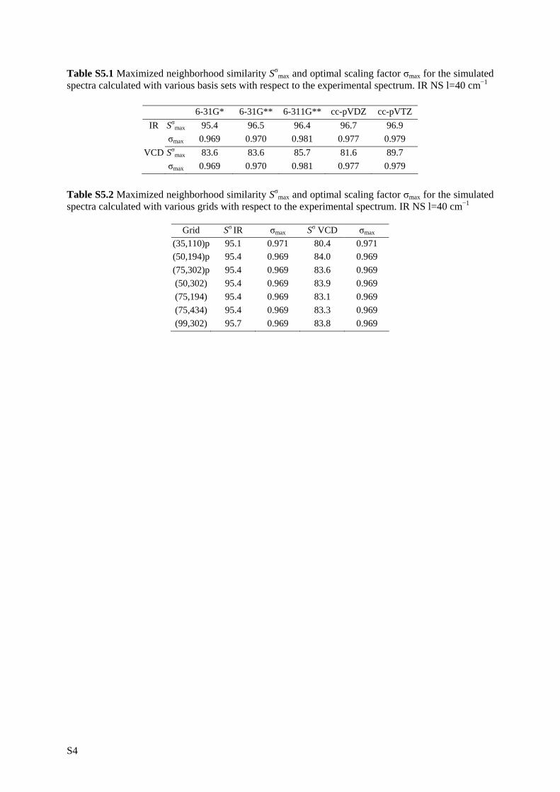
S4
Table S5.1 Maximized neighborhood similarity Sσmax and optimal scaling factor σmax for the simulated spectra calculated with various basis sets with respect to the experimental spectrum. IR NS l=40 cm−1
6-31G* 6-31G** 6-311G** cc-pVDZ cc-pVTZ IR Sσmax 95.4 96.5 96.4 96.7 96.9
σmax 0.969 0.970 0.981 0.977 0.979 VCD Sσmax 83.6 83.6 85.7 81.6 89.7
σmax 0.969 0.970 0.981 0.977 0.979 Table S5.2 Maximized neighborhood similarity Sσmax and optimal scaling factor σmax for the simulated spectra calculated with various grids with respect to the experimental spectrum. IR NS l=40 cm−1
Grid Sσ IR σmax Sσ VCD σmax
(35,110)p 95.1 0.971 80.4 0.971 (50,194)p 95.4 0.969 84.0 0.969 (75,302)p 95.4 0.969 83.6 0.969 (50,302) 95.4 0.969 83.9 0.969 (75,194) 95.4 0.969 83.1 0.969 (75,434) 95.4 0.969 83.3 0.969 (99,302) 95.7 0.969 83.8 0.969

S5
Chapter 6
Table S6.1 Assignment of the experimental peaks of (+)-1 (B3LYP/6-31G*) Table S6.2 Assignment of the experimental peaks of (+)-1 (B3LYP/cc-pVTZ) Table S6.3 Assignment of the experimental peaks of (+)-2 (B3LYP/6-31G*) Table S6.4 Assignment of the experimental peaks of (+)-2 (B3LYP/cc-pVTZ) Table S6.5 Assignment of the experimental peaks of (−)-3 (B3LYP/6-31G*) Table S6.6 Assignment of the experimental peaks of (−)-3 (B3LYP/cc-pVTZ) Table S6.7 Neighborhood similarity Sσ for theoretical versus experimental IR and VCD spectra using different functionals Figure S6.1 IR absorption and VCD spectrum for (+)-1, (+)-2 and (−)-3, including Lorentzian fit and residual fitting error Figure S6.2 Simulated (1S,8S)-1 IR DFT/6-31G* for different functionals and experimental spectra Figure S6.3 (1S,8S)-1 VCD DFT/6-31G* for different functionals and experimental spectra. Figure S6.4 Simulated (S)-2 IR DFT/6-31G* for different functionals and experimental spectra. Figure S6.5 Simulated (S)-2 VCD DFT/6-31G* for different functionals and experimental spectra. Figure S6.6 Simulated (1R,2S,7S,8R)-3 IR DFT/6-31G* for different functionals and experimental spectra. Figure S6.7 Simulated (1R,2S,7S,8R)-3 IR DFT/6-31G* for different functionals and experimental spectra. Figure S6.8 Mid IR and OH stretch region for (+)-2 in three different solvents. General experimental methods

S6
Table S6.1 Assignment of the experimental peaks of (+)-1 based on the B3LYP/6-31G* simulated spectra. The experimental values of the vibrational frequencies (in cm−1), dipole (D in 10−40 esu2cm2) and rotational strength (R in 10−44 esu2cm2) were Lorentzian fitted. Fundamentals are labeled according to the minimum (a ≡ eGeG’ b ≡ eG’eT). Calculated values of D and R are Boltzmann weighed according to Table 6.1a.
Experimental B3LYP/6-31G* Fund
freq D R freq* D R 34a 1024.83 104.57 14.28 1024.48 27.07 24.45 34b 1034.65 ┴ −12.33 1030.40 9.83 −6.09 35a 1042.73 201.76 116.04 1035.31 169.35 10.25 35b ┴ ┴ 1041.08 3.83 2.48 36b 1054.98 75.22 106.26 1045.43 15.79 14.56 36a 1064.06 165.79 ┴ 1047.04 93.08 53.82 37b 1075.09 339.49 −137.13 1085.52 47.18 3.94 37a ┴ ┴ 1085.62 289.06 −2.34 38a 1130.65 17.29 −28.06 1119.84 21.77 −38.96 38b 1137.29 30.95 │ 1128.28 3.87 −3.02 39a │ ┴ 1128.49 8.86 −3.15 39b 1139.53 │ 18.17 1132.46 1.72 2.60 40a ┴ ┴ 1133.15 8.04 12.59 40b 1147.58 17.66 −36.21 1143.99 3.45 −2.93 41b 1165.08 28.78 15.96 1148.67 4.14 8.63 41a ┴ ┴ 1151.12 7.42 11.04 42b 1187.64 49.24 39.94 1173.48 0.55 0.05 42a ┴ ┴ 1174.57 1.03 1.45 43b 1204.16 48.13 55.55 1185.42 21.25 7.56 43a │ │ 1193.64 3.87 2.47 44b ┴ ┴ 1201.03 11.38 1.46 44a 1226.20 22.62 −54.94 1218.27 41.35 −2.22 45a 1229.94 87.14 │ 1221.88 16.76 −14.89 45b │ │ 1222.81 1.96 −1.82 46b │ │ 1224.50 3.00 −3.35 46a ┴ ┴ 1231.82 3.35 −5.41 47a 1256.29 83.32 −66.89 1258.70 38.79 −42.67 47b │ │ 1260.17 5.49 −7.41 48b │ │ 1272.35 0.77 −2.19 48a ┴ ┴ 1275.07 16.58 −10.49 49a 1280.89 27.34 24.52 1279.92 21.74 13.33 49b ┴ ┴ 1280.69 0.68 0.59 50b 1288.31 57.44 −47.59 1289.41 1.04 −2.47 50a │ ┴ 1289.77 19.59 −8.56 51a 1295.42 ┴ 13.93 1296.22 7.77 4.69 51b 1304.38 66.34 │ 1300.70 4.95 −0.85 52a │ │ 1304.39 19.61 2.72 52b ┴ ┴ 1311.45 6.36 −1.91

S7
53a 1325.15 133.79 93.86 1328.19 225.14 20.39 53b 1334.61 92.61 │ 1331.55 44.68 0.58 54a │ │ 1340.82 19.91 −1.80 54b ┴ │ 1344.28 0.32 −0.05 55b 1379.26 46.53 ┴ 1383.32 6.76 −3.17 55a 1388.30 115.43 −66.80 1391.64 167.52 −28.64 56a 1388.85 ┴ −84.63 1409.11 42.26 −29.47 56b 1402.34 52.32 │ 1416.98 6.86 −3.94 57a 1420.35 13.13 │ 1434.65 1.81 −2.65 57b ┴ ┴ 1439.29 0.61 −0.63 58a 1438.23 45.75 4.62 1455.09 41.22 15.18 58b ┴ ┴ 1456.28 7.83 3.45 59a 1453.52 78.36 −28.40 1465.29 1.44 −1.73 59b ┴ ┴ 1466.48 0.31 −0.45 60a 1468.36 85.65 29.74 1469.27 35.92 16.20 60b ┴ ┴ 1469.87 5.79 2.66 * scaled with factor 0.967 Correlation coefficients – D: 72% / R: 47%
Table S6.2 Assignment of the experimental peaks of (+)-1 based on the B3LYP/cc-pVTZ simulated spectra. The experimental values of the vibrational frequencies (in cm−1), dipole (D in 10−40 esu2cm2) and rotational strength (R in 10−44 esu2cm2) were Lorentzian fitted. Fundamentals are labeled according to the minimum (a ≡ eGeG’ b ≡ eG’eT). Calculated values of D and R are Boltzmann weighed according to Table 6.1b.
Experimental B3LYP/cc-pVTZ Fund
freq D R freq* D R 34a 1024.83 104.57 14.28 1025.47 36.22 34.00 34b 1034.65 ┴ −12.33 1031.87 21.37 −10.81 35a 1042.73 201.76 116.04 1036.53 186.82 17.44 35b ┴ ┴ 1039.70 18.94 15.34 36a 1054.98 75.22 106.26 1047.37 49.35 24.85 36b 1064.06 165.79 ┴ 1046.22 13.71 11.46 37a 1075.09 339.49 −137.13 1076.72 272.24 −9.80 37b ┴ ┴ 1076.68 75.90 4.05 38a 1130.65 17.29 −28.06 1123.10 18.43 −31.33 38b 1137.29 30.95 │ 1132.21 3.91 −3.48 39a │ ┴ 1132.26 5.28 3.95 39b 1139.53 │ 18.17 1135.90 5.87 4.76 40a ┴ ┴ 1136.54 12.24 11.26 40b 1147.58 17.66 −36.21 1147.10 6.51 −2.79 41a 1165.08 28.78 15.96 1157.47 8.23 4.92 41b ┴ ┴ 1155.84 4.57 10.55 42a 1187.64 49.24 39.94 1178.80 0.83 1.62 42b ┴ ┴ 1177.42 1.96 0.05 43a 1204.16 48.13 55.55 1202.88 4.60 0.97 43b │ │ 1187.34 36.87 11.25 44a ┴ ┴ 1221.37 28.76 1.89 44b 1226.20 22.62 −54.94 1206.79 4.52 0.59
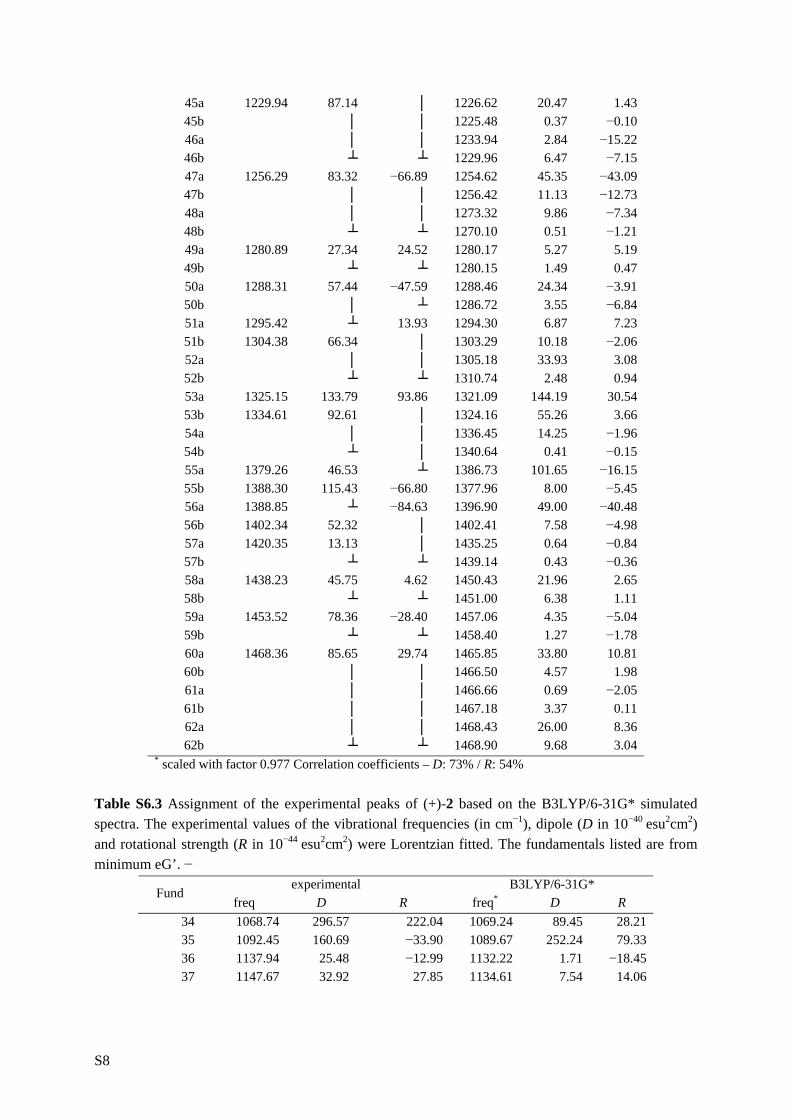
S8
45a 1229.94 87.14 │ 1226.62 20.47 1.43 45b │ │ 1225.48 0.37 −0.10 46a │ │ 1233.94 2.84 −15.22 46b ┴ ┴ 1229.96 6.47 −7.15 47a 1256.29 83.32 −66.89 1254.62 45.35 −43.09 47b │ │ 1256.42 11.13 −12.73 48a │ │ 1273.32 9.86 −7.34 48b ┴ ┴ 1270.10 0.51 −1.21 49a 1280.89 27.34 24.52 1280.17 5.27 5.19 49b ┴ ┴ 1280.15 1.49 0.47 50a 1288.31 57.44 −47.59 1288.46 24.34 −3.91 50b │ ┴ 1286.72 3.55 −6.84 51a 1295.42 ┴ 13.93 1294.30 6.87 7.23 51b 1304.38 66.34 │ 1303.29 10.18 −2.06 52a │ │ 1305.18 33.93 3.08 52b ┴ ┴ 1310.74 2.48 0.94 53a 1325.15 133.79 93.86 1321.09 144.19 30.54 53b 1334.61 92.61 │ 1324.16 55.26 3.66 54a │ │ 1336.45 14.25 −1.96 54b ┴ │ 1340.64 0.41 −0.15 55a 1379.26 46.53 ┴ 1386.73 101.65 −16.15 55b 1388.30 115.43 −66.80 1377.96 8.00 −5.45 56a 1388.85 ┴ −84.63 1396.90 49.00 −40.48 56b 1402.34 52.32 │ 1402.41 7.58 −4.98 57a 1420.35 13.13 │ 1435.25 0.64 −0.84 57b ┴ ┴ 1439.14 0.43 −0.36 58a 1438.23 45.75 4.62 1450.43 21.96 2.65 58b ┴ ┴ 1451.00 6.38 1.11 59a 1453.52 78.36 −28.40 1457.06 4.35 −5.04 59b ┴ ┴ 1458.40 1.27 −1.78 60a 1468.36 85.65 29.74 1465.85 33.80 10.81 60b │ │ 1466.50 4.57 1.98 61a │ │ 1466.66 0.69 −2.05 61b │ │ 1467.18 3.37 0.11 62a │ │ 1468.43 26.00 8.36 62b ┴ ┴ 1468.90 9.68 3.04
* scaled with factor 0.977 Correlation coefficients – D: 73% / R: 54% Table S6.3 Assignment of the experimental peaks of (+)-2 based on the B3LYP/6-31G* simulated spectra. The experimental values of the vibrational frequencies (in cm−1), dipole (D in 10−40 esu2cm2) and rotational strength (R in 10−44 esu2cm2) were Lorentzian fitted. The fundamentals listed are from minimum eG’. −
experimental B3LYP/6-31G* Fund
freq D R freq* D R 34 1068.74 296.57 222.04 1069.24 89.45 28.21 35 1092.45 160.69 −33.90 1089.67 252.24 79.33 36 1137.94 25.48 −12.99 1132.22 1.71 −18.45 37 1147.67 32.92 27.85 1134.61 7.54 14.06

S9
38 ┴ ┴ 1138.62 24.39 19.05 39 1179.41 49.47 −42.38 1168.36 43.47 −22.67 40 1194.59 57.49 15.10 1190.49 41.42 11.15 41 1213.49 53.64 2.13 1206.76 0.52 5.33 42 ┴ ┴ 1212.71 11.34 9.29 43 1235.08 72.54 −111.60 1227.28 108.41 −42.98 44 1249.79 104.86 38.00 1247.91 60.56 28.66 45 1257.26 30.37 −48.84 1257.10 100.35 −74.32
1259.64 73.19 ┴ ┴ ┴ 46 1278.90 125.80 −65.43 1277.09 131.08 −6.35 47 1286.09 78.04 −18.54 1284.74 13.93 −16.92 48 1299.15 83.38 −2.72 1298.52 13.48 −3.19 49 1331.65 149.02 84.48 1332.26 214.69 21.33 50 1341.54 44.48 −32.00 1345.75 11.97 −23.31 51 1390.98 55.57 6.17 1409.29 93.06 4.86 52 1406.57 86.00 −11.84 1426.98 93.42 −10.57 53 1416.32 41.12 −6.10 1437.65 34.33 −3.52
1427.01 ┴ 2.09 ┴ ┴ 54 1442.73 57.15 6.53 1456.68 78.81 24.64 55 1438.93 70.21 ┴ 1466.39 43.45 7.41 56 1454.00 74.69 −10.08 1472.05 14.76 9.22 57 1473.41 116.00 23.56 1477.54 7.52 −3.16 58 1586.97 104.35 - 1583.22 66.62 −1.67 59 1613.42 154.70 −17.25 1601.36 86.44 −1.50 60 1686.50 1215.25 151.90 1713.72 608.98 27.80
* scaled with factor 0.967 Correlation coefficients – D: 79% / R:23% Table S6.4 Assignment of the experimental peaks of (+)-2 based on the B3LYP/cc-pVTZ simulated spectra. The experimental values of the vibrational frequencies (in cm−1), dipole (D in 10−40 esu2cm2) and rotational strength (R in 10−44 esu2cm2) were Lorentzian fitted. The fundamentals listed are from minimum eG’.
experimental B3LYP/cc-pVTZ Fund
freq D R freq* D R 33 1026.20 66.25 −103.77 1023.92 68.95 −29.65 34 1068.74 296.57 222.04 1075.34 97.67 71.77 35 1092.45 160.69 −33.90 1086.02 264.70 36.88 36 1137.94 25.48 −12.99 1135.91 0.89 −11.24 37 1147.67 32.92 27.85 1139.12 3.48 4.59 38 ┴ ┴ 1144.39 31.47 20.78 39 1179.41 49.47 −42.38 1172.38 46.84 −23.81 40 1194.59 57.49 15.10 1193.96 40.42 12.98 41 1213.49 53.64 2.13 1212.66 0.32 6.13 42 ┴ ┴ 1218.65 5.95 0.41 43 1235.08 72.54 −111.60 1232.60 92.22 −46.70 44 1249.79 104.86 38.00 1247.34 92.79 38.55 45 1257.26 30.37 −48.84 1256.37 92.25 −70.55
1259.64 73.19 ┴ ┴ ┴ 46 1278.90 125.80 −65.43 1277.02 102.59 −11.25

S10
47 1286.09 78.04 −18.54 1283.63 23.51 −23.90 48 1299.15 83.38 −2.72 1301.51 11.16 −6.08 49 1331.65 149.02 84.48 1328.97 168.95 25.48 50 1341.54 44.48 −32.00 1341.69 11.04 −21.88 51 1390.98 55.57 6.17 1402.88 106.45 10.34 52 1406.57 86.00 −11.84 1418.96 42.00 −7.12 53 1416.32 41.12 −6.10 1434.56 61.77 0.84
1427.01 ┴ 2.09 ┴ ┴ 54 1442.73 57.15 6.53 1451.52 46.27 9.61 55 1438.93 70.21 ┴ 1457.56 34.08 0.18 56 1454.00 74.69 −10.08 1468.08 2.39 −5.60 57 1473.41 116.00 23.56 1471.41 70.55 23.85 58 1586.97 104.35 - 1586.07 71.63 −0.55 59 1613.42 154.70 −17.25 1603.03 90.97 1.47 60 1686.50 1215.25 151.90 1707.75 670.62 35.77
* scaled with factor 0.977 Correlation coefficients – D: 86% / R: 64%
Table S6.5 Assignment of the experimental peaks of (−)-3 based on the B3LYP/6-31G* simulated spectra. The experimental values of the vibrational frequencies (in cm−1), dipole (D in 10−40 esu2cm2) and rotational strength (R in 10−44 esu2cm2) were Lorentzian fitted.
experimental B3LYP/6-31G* Fund
freq D R freq* D R 34 1088.34 9.94 −7.91 1066.00 2.47 −6.54 35 ┴ ┴ 1071.93 2.63 −3.41 36 1131.78 17.90 5.81 1126.37 10.51 0.38 37 1165.18 7.28 43.73 1162.92 12.36 −1.15 38 1167.03 28.66 ┴ 1163.87 2.51 4.88 39 1194.46 6.46 38.53 1180.22 0.96 1.96 40 1207.20 50.50 −56.82 1198.71 18.71 −15.41 41 ┴ ┴ 1204.84 14.03 −22.18 42 1228.58 23.08 31.82 1219.22 13.94 23.09 43 1232.30 68.18 −49.03 1223.08 25.13 −38.50 44 1248.24 17.30 9.20 1243.04 24.79 0.19 45 1282.52 20.61 3.67 1279.92 4.67 4.14 46 1288.05 ┴ 22.77 1280.34 3.55 8.13 47 1327.72 16.19 2.83 1312.62 6.76 6.66 48 1351.85 18.10 −17.56 1338.69 1.25 −5.94 49 1363.04 7.60 32.49 1376.14 25.68 −32.90 50 1367.16 45.17 41.95 1376.29 44.42 78.25 51 1422.65 3.87 33.84 1441.44 9.48 −6.93 52 1431.12 25.48 20.00 1441.67 27.21 9.54 53 1454.67 31.83 11.82 1453.16 2.19 2.51 54 1455.85 │ 3.32 1454.53 31.83 15.33
1459.12 ┴ 25.65 ┴ ┴ 55 1601.74 23.52 −10.89 1590.68 0.44 −3.94 56 1650.93 21.00 −5.35 1620.19 0.63 −1.33
* scaled with factor 0.967 Correlation coefficients – D: 27% / R: 28%

S11
Table S6.6 Assignment of the experimental peaks of (−)-3 based on the B3LYP/cc-pVTZ simulated spectra. The experimental values of the vibrational frequencies (in cm−1), dipole (D in 10−40 esu2cm2) and rotational strength (R in 10−44 esu2cm2) were Lorentzian fitted.
experimental B3LYP/cc-pVTZ Fund
freq D R freq* D R 33 1037.20 95.81 −18.23 1031.95 74.06 −18.84 34 1088.34 9.94 −7.91 1080.92 2.76 −6.81 35 ┴ ┴ 1085.69 1.77 −0.74 36 1131.78 17.90 5.81 1130.17 12.13 0.01 37 1165.18 7.28 43.73 1166.93 11.23 3.20 38 1167.03 28.66 ┴ 1167.35 3.85 7.51 39 1194.46 6.46 38.53 1190.18 1.96 3.50 40 1207.20 50.50 −56.82 1202.51 20.32 −3.33 41 ┴ ┴ 1207.05 18.27 −29.84 42 1228.58 23.08 31.82 1222.13 7.75 19.53 43 1232.30 68.18 −49.03 1228.94 26.90 −45.83 44 1248.24 17.30 9.20 1240.69 28.86 4.58 45 1282.52 20.61 3.67 1279.20 8.49 6.33 46 1288.05 ┴ 22.77 1279.67 0.86 7.23 47 1327.72 16.19 2.83 1314.45 4.42 5.23 48 1351.85 18.10 −17.56 1334.33 1.85 −7.17 49 1363.04 7.60 32.49 1369.96 41.21 65.74 50 1367.16 45.17 41.95 1371.94 20.96 −28.85 51 1422.65 3.87 33.84 1431.08 17.38 −3.13 52 1431.12 25.48 20.00 1431.33 23.68 5.64 53 1454.67 31.83 11.82 1452.46 0.73 1.88 54 1455.85 │ 3.32 1456.42 43.03 20.82
1459.12 ┴ 25.65 ┴ ┴ 55 1601.74 23.52 −10.89 1593.71 1.00 −4.67 56 1650.93 21.00 −5.35 1622.18 0.59 −1.27
* scaled with factor 0.977 Correlation coefficients – D: 45% / R: 38%

S12
Table S6.7 Neighborhood similarity Sσ (Equation 6.2) and maximizing scaling factor (for default IR overlap) for theoretical versus experimental IR and VCD spectra using different functionals with the 6-31G* basis set for respectively 1 (a), 2 (b) and 3 (c).
a functional Sσ IR Sσ VCD σ B1LYP 0.938 0.758 0.954 B3LYP 0.936 0.746 0.960 B3P86 0.907 0.702 0.942 B3PW91 0.911 0.717 0.945 B98 0.925 0.759 0.955 BHandH 0.854 0.511 0.901 BHandHLYP 0.912 0.723 0.906 MPW1PW91 0.905 0.690 0.934 PBE1PBE 0.903 0.670 0.932
b functional Sσ IR Sσ VCD σ B1LYP 0.913 0.731 0.944 B3LYP 0.920 0.743 0.952 B3P86 0.916 0.622 0.941 B3PW91 0.914 0.624 0.942 B98 0.894 0.646 0.944 BHandH 0.565 0.453 0.900 BHandHLYP 0.855 0.628 0.901 MPW1PW91 0.909 0.592 0.931 PBE1PBE 0.908 0.566 0.930
c functional Sσ IR Sσ VCD σ B1LYP 0.864 0.597 0.969 B3LYP 0.871 0.622 0.975 B3P86 0.899 0.637 0.969 B3PW91 0.897 0.634 0.970 B98 0.891 0.648 0.977 BHandH 0.861 0.550 0.938 BHandHLYP 0.875 0.490 0.930 MPW1PW91 0.895 0.606 0.962 PBE1PBE 0.895 0.604 0.964

S13
1500 1400 1300 1200 1100 100000
25
5050
75
100100
125
150150
175
200200
225
250250 ExperimentLorentzian fitted
ν
ε
Error
1500 1400 1300 1200 1100 1000
-0.02
-0.02-0.02
-0.01
-0.01-0.01
-0.00
0.000.00
0.01
0.010.01
0.01
0.020.02 ExperimentLorentzian fitted
ν
Δε
Error
1700 1600 1500 1400 1300 1200 1100 100000
50100100150200200250300300350400400450500500550600600650700700750
ExperimentLorentzian fitted
ν
ε
Error
1600 1500 1400 1300 1200 110000
10
2020
30
4040
50
6060
70
8080
90
100100
110
120120 ExperimentLorentzian fitted
ν
ε
Error
1600 1500 1400 1300 1200 1100-0.02-0.02
-0.01
-0.01-0.01
-0.01
0.000.00
0.01
0.010.01
0.01
0.020.02
0.03 ExperimentLorentzian fitted
ν
Δε
Error
(+)-1 (+)-1
(+)-2(+)-2
(-)-3(-)-3
1600 1400 1200 1000
-0.02-0.02
-0.01
0.000.00
0.01
0.020.02
0.03
0.040.04ExperimentLorentzian fitted
ν
Δε
Error
Figure S6.1 Unpolarized IR absorption and VCD spectrum for (+)-1, (+)-2 and (−)-3, including Lorentzian fit and residual fitting error (absorptions and differential absorptions in molar absorptivity units).
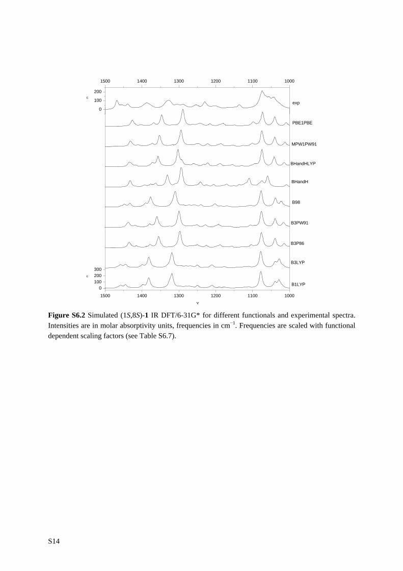
S14
1500 1400 1300 1200 1100 1000
0100200300
ν
B3LYP
B3PW91
B3P86
B1LYP
ε
BHandH
BHandHLYP
MPW1PW91
ε
B98
exp
PBE1PBE
0
100
200
1500 1400 1300 1200 1100 1000
Figure S6.2 Simulated (1S,8S)-1 IR DFT/6-31G* for different functionals and experimental spectra. Intensities are in molar absorptivity units, frequencies in cm−1. Frequencies are scaled with functional dependent scaling factors (see Table S6.7).

S15
1500 1400 1300 1200 1100 1000-0.02-0.010.000.010.020.03
ν
Δ ε
Δ ε
exp
B3LYP
B3PW91
B3P86
B1LYP
BHandH
BHandHLYP
MPW1PW91
B98
PBE1PBE
-0.03-0.02-0.010.000.010.02
1500 1400 1300 1200 1100 1000
Figure S6.3 Simulated (1S,8S)-1 VCD DFT/6-31G* for different functionals and experimental spectra. Intensities are in molar absorptivity units, frequencies in cm−1. Frequencies are scaled with functional dependent scaling factors (see Table S6.7).

S16
1700 1600 1500 1400 1300 1200 1100 10000
100200300
ν
B3LYP
B3PW91
B3P86
B1LYP
ε
BHandH
BHandHLYP
MPW1PW91
ε
B98
exp
PBE1PBE
0100200300
1700 1600 1500 1400 1300 1200 1100 1000
Figure S6.4 Simulated (S)-2 IR DFT/6-31G* for different functionals and experimental spectra. Intensities are in molar absorptivity units, frequencies in cm−1. Frequencies are scaled with functional dependent scaling factors (see Table S6.7).

S17
1700 1600 1500 1400 1300 1200 1100 1000-0.03-0.02-0.010.000.010.020.03
ν
Δ ε
Δ ε
exp
B3LYP
B3PW91
B3P86
B1LYP
BHandH
BHandHLYP
MPW1PW91
B98
PBE1PBE-0.02-0.010.000.010.020.030.04
1700 1600 1500 1400 1300 1200 1100 1000
Figure S6.5 Simulated (S)-2 VCD DFT/6-31G* for different functionals and experimental spectra. Intensities are in molar absorptivity units, frequencies in cm−1. Frequencies are scaled with functional dependent scaling factors (see Table S6.7).

S18
1500 1400 1300 1200 1100 10000
255075
100
ν
B3LYP
B3PW91
B3P86
B1LYP
ε
BHandH
BHandHLYP
MPW1PW91
ε
B98
exp
PBE1PBE
0255075
100
1500 1400 1300 1200 1100 1000
Figure S6.6 Simulated (1R,2S,7S,8R)-3 IR DFT/6-31G* for different functionals and experimental spectra. Intensities are in molar absorptivity units, frequencies in cm−1. Frequencies are scaled with functional dependent scaling factors (see Table S6.7).

S19
1600 1500 1400 1300 1200 1100
-0.010.000.010.020.03
ν
Δ ε
Δ ε
exp
B3LYP
B3PW91
B3P86
B1LYP
BHandH
BHandHLYP
MPW1PW91
B98
PBE1PBE
-0.02-0.010.000.010.02
1600 1500 1400 1300 1200 1100
Figure S6.7 Simulated (1R,2S,7S,8R)-3 IR DFT/6-31G* for different functionals and experimental spectra. Intensities are in molar absorptivity units, frequencies in cm−1. Frequencies are scaled with functional dependent scaling factors (see Table S6.7).

S20
1800 1700 1600 1500 1400 1300 1200 1100 10000.0
0.2
0.4
0.6
CDCl3 CD2Cl2 Cl2C=CCl2
3700 3600 3500 3400 3300 32000.0
0.1
0.2
A
A
ν
ν Figure S6.8 Mid IR and OH stretch region for (+)-2 in three different solvents.
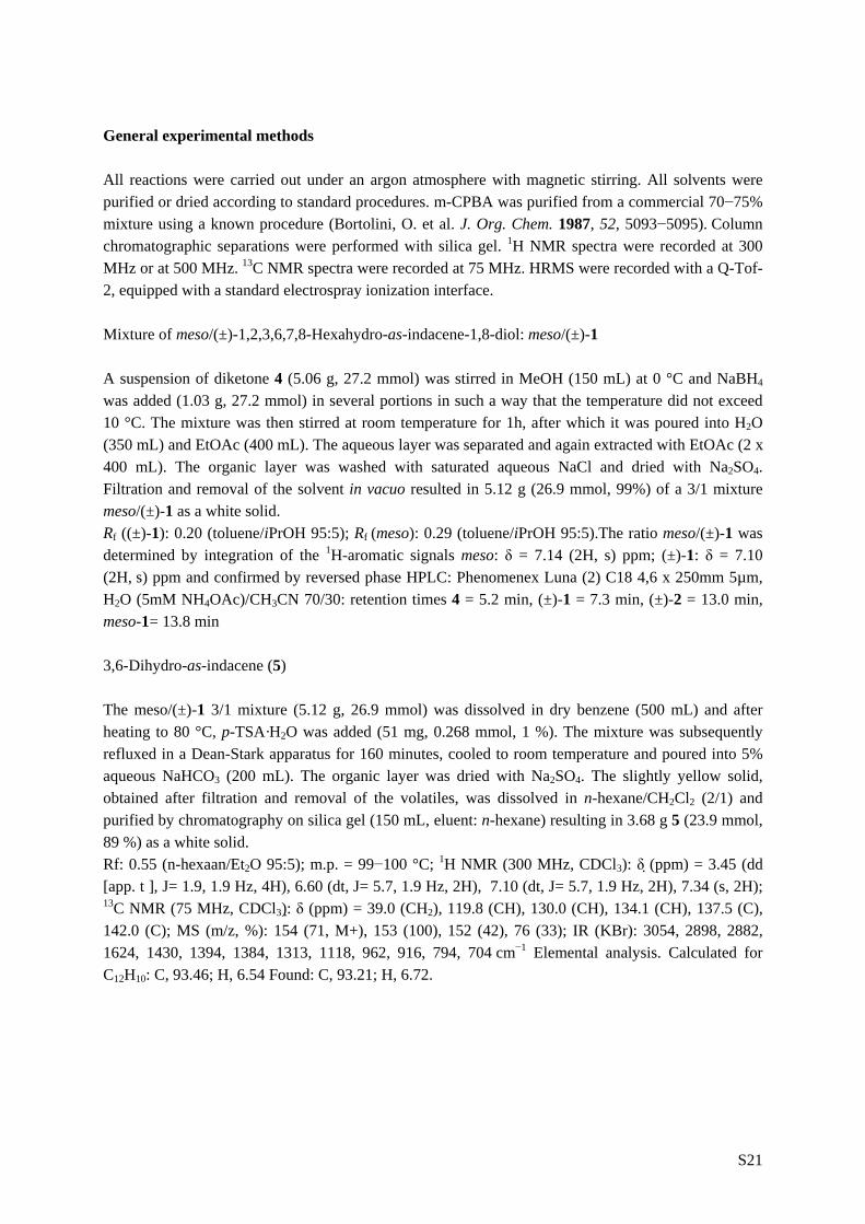
S21
General experimental methods
All reactions were carried out under an argon atmosphere with magnetic stirring. All solvents were purified or dried according to standard procedures. m-CPBA was purified from a commercial 70−75% mixture using a known procedure (Bortolini, O. et al. J. Org. Chem. 1987, 52, 5093−5095). Column chromatographic separations were performed with silica gel. 1H NMR spectra were recorded at 300 MHz or at 500 MHz. 13C NMR spectra were recorded at 75 MHz. HRMS were recorded with a Q-Tof-2, equipped with a standard electrospray ionization interface. Mixture of meso/(±)-1,2,3,6,7,8-Hexahydro-as-indacene-1,8-diol: meso/(±)-1 A suspension of diketone 4 (5.06 g, 27.2 mmol) was stirred in MeOH (150 mL) at 0 °C and NaBH4 was added (1.03 g, 27.2 mmol) in several portions in such a way that the temperature did not exceed 10 °C. The mixture was then stirred at room temperature for 1h, after which it was poured into H2O (350 mL) and EtOAc (400 mL). The aqueous layer was separated and again extracted with EtOAc (2 x 400 mL). The organic layer was washed with saturated aqueous NaCl and dried with Na2SO4. Filtration and removal of the solvent in vacuo resulted in 5.12 g (26.9 mmol, 99%) of a 3/1 mixture meso/(±)-1 as a white solid. Rf ((±)-1): 0.20 (toluene/iPrOH 95:5); Rf (meso): 0.29 (toluene/iPrOH 95:5).The ratio meso/(±)-1 was determined by integration of the 1H-aromatic signals meso: δ = 7.14 (2H, s) ppm; (±)-1: δ = 7.10 (2H, s) ppm and confirmed by reversed phase HPLC: Phenomenex Luna (2) C18 4,6 x 250mm 5µm, H2O (5mM NH4OAc)/CH3CN 70/30: retention times 4 = 5.2 min, (±)-1 = 7.3 min, (±)-2 = 13.0 min, meso-1= 13.8 min 3,6-Dihydro-as-indacene (5) The meso/(±)-1 3/1 mixture (5.12 g, 26.9 mmol) was dissolved in dry benzene (500 mL) and after heating to 80 °C, p-TSA·H2O was added (51 mg, 0.268 mmol, 1 %). The mixture was subsequently refluxed in a Dean-Stark apparatus for 160 minutes, cooled to room temperature and poured into 5% aqueous NaHCO3 (200 mL). The organic layer was dried with Na2SO4. The slightly yellow solid, obtained after filtration and removal of the volatiles, was dissolved in n-hexane/CH2Cl2 (2/1) and purified by chromatography on silica gel (150 mL, eluent: n-hexane) resulting in 3.68 g 5 (23.9 mmol, 89 %) as a white solid. Rf: 0.55 (n-hexaan/Et2O 95:5); m.p. = 99−100 °C; 1H NMR (300 MHz, CDCl3): δ (ppm) = 3.45 (dd [app. t ], J= 1.9, 1.9 Hz, 4H), 6.60 (dt, J= 5.7, 1.9 Hz, 2H), 7.10 (dt, J= 5.7, 1.9 Hz, 2H), 7.34 (s, 2H); 13C NMR (75 MHz, CDCl3): δ (ppm) = 39.0 (CH2), 119.8 (CH), 130.0 (CH), 134.1 (CH), 137.5 (C), 142.0 (C); MS (m/z, %): 154 (71, M+), 153 (100), 152 (42), 76 (33); IR (KBr): 3054, 2898, 2882, 1624, 1430, 1394, 1384, 1313, 1118, 962, 916, 794, 704 cm−1 Elemental analysis. Calculated for C12H10: C, 93.46; H, 6.54 Found: C, 93.21; H, 6.72.

S22
(−)365-(1R,2S,7S,8R)-1,2,7,8-di-epoxy-3,6-dihydro-as-indacene (3) 4-Methylmorpholine N-oxide (381.5 mg, 3.26 mmol, 5 eq) and Mn-(R,R)-Salen (20.7 mg, 0.033 mmol, 5%) were dissolved in CH2Cl2 (7.5 mL) after which the mixture was cooled to −78 °C. Diene 5 (100.6 mg, 0.65 mmol) was added at −78 °C and after dissolution, m-CPBA (~90% purity, 378 mg, 2.0 mmol, 3 eq) was added in one portion. After 110 minutes, 1N aqueous NaOH (2 mL) was added and the mixture was then poured into 1N aqueous NaOH (8 mL) and CH2Cl2 (10 mL). The organic layer was washed with saturated aqueous NaHCO3 (10 mL) followed by saturated aqueous NaCl (20 mL). The combined H2O layers were extracted with CH2Cl2 (2 x 20mL). The combined organic layers were dried on Na2SO4, filtered, concentrated and filtered over silica gel (2 mL, pre-treated with a CH2Cl2/1% NEt3 mixture). This resulted in 128 mg of a pale yellow solid. The product was recrystallized from toluene to obtain 93 mg of a white solid 3 (0.50 mmol, 77%, >98% ee, >98% de). The product can be sublimated at 150 °C/0.2−0.3 mmHg. Sublimation >200 °C, 25
Dα = −0.8, 25365α = −128.6 (c=0.99, CHCl3). 1H NMR (500 MHz, CDCl3):
δ (ppm) = 2.99 (dd, J= 17.5, 2.7 Hz, 2H), 3.20 (d, J= 17.5 Hz, 2H) 4.18 (dd [app. t], J= 2.7, 2.7 Hz, 2H), 4.47 (dd, J= 2.7, 0.9 Hz, 2H), 7.12 (2H, s) ppm; 13C NMR (75 MHz, CDCl3): δ (ppm) = 34.3 (CH2), 57.2 (CH), 58.2 (CH), 125.9 (CH), 137.9 (C), 141.9 (C); MS (m/z, %): 186 (100), 158 (50), 130 (72), 129 (60), 128 (68), 115 (58) Analysis on Chiralcel OD−H column, see supporting information: IR (CDCl3) : 3050, 2914, 2252, 1459, 1420, 1367, 1231, 1207, 1037, 1005, 983, 910, 831, 808, 753, 714, 622 cm−1; HRMS found: [M+H]+: 187.0761; calculated for C12H11O2: 187.0758. Elemental analysis. Calculated for C12H10O2: C, 77.40; H, 5.41 Found: C, 77.31; H, 5.50. (1S,8S)-1,2,3,6,7,8-Hexahydro-as-indacene-1,8-diol 1 and (8S)-8-hydroxy-3,6,7,8-tetrahydro-2H-as-indacen-1-one 2: A mixture of [RuCl2(η6-cymene)]2, (226 mg, 0.369 mmol), (S,S)-Ts-DPEN (282 mg, 0.770 mmol) and NEt3 (145 μl, 1.04 mmol) was dissolved in degassed DMF (70 mL) and stirred for 1 h at 80 °C in a closed vessel under argon. At room temperature, this solution was added to 4 (4.71 g, 0.0253 mol) in a flask equipped with an argon balloon. After addition of HCOOH:NEt3 (5:2 azeotrope; 35 mL) the mixture was stirred for 96 h. The solution was poured into H2O (500 mL) and extracted with toluene (8 x 500 mL). After drying with Na2SO4, filtration and evaporation of the volatiles, the crude material (5.72 g) was purified by chromatography on silica gel with gradient elution (iPrOH/toluene, 1−5 %) resulting in three fractions: 0.43 g of an apolar fraction containing (8S)-2, 0.134 g meso-1 (0.704 mmol, ~ 2 %) and 4.2 g of a more polar fraction containing (1S,8S)-1 (>99 % ee). The polar fraction was further purified by crystallization from nhexane/benzene 50/50 resulting in 3.905 g (1S,8S)-1 (20.53 mmol, 81 %, >99 % ee). The apolar fraction was further purified by chromatography on silica gel (pentane/acetone, 90/10) resulting in 247 mg (8S)-2 (1.312 mmol, 5 %, 98 % ee) Data for (1S,8S)-1 from ref 14 (Chapter 6): For analytical purposes the product was crystallized twice from CH2Cl2. Rf : 0.20 (tolueen/iPrOH 95:5), mp = 155.5−156.5 °C; 20
Dα = +70.5 (c 1.09, CHCl3); 1H
NMR (500 MHz, CDCl3): δ (ppm) = 1.91 (2H, dddd [app. dq], J= 8.4, 9.3, 9.3, 12.5), 2.56 (2H, dddd,

S23
J = 2.0, 7.1, 7.5, 12.5), 2.77 (2H, ddd, J = 7.5, 9.3, 15.0), 2.94 (2H, ddd, J = 2.0, 9.3, 15.0), 5.47 (2H, dd [app. t], J = 7.1, 8.4), 7.10 (2H, s); 13C NMR (125 MHz, CDCl3): δ (ppm) = 29.7 (CH2), 35.9 (CH2), 75.6 (CH), 124.5 (CH), 140.6 (C), 141.1 (C) ppm; MS (m/z, %): 115 (40), 128 (67), 129 (100), 144 (74), 153 (48), 154 (34), 171 (28), 172 (64), 190 (M+, 8); ES−MS: 129.0 (16), 155.0 (29) [M-2xH2O+H]+, 173.0 (100) [M-H20+H]+, 213.0 (6) [M+Na]+, IR (CDCl3) 2360, 2340, 2254, 1794, 1643, 1561, 1469, 1383, 1329, 1230, 1166, 1095, 1075, 918, 909, 902, 736, 651, 625, 543 cm−1. Elemental analysis. Calculated for C12H14O2: C, 75.76; H, 7.42 Found: C, 75.68; H, 7.51 HPLC: Chiralcel OD−H column, solvent: n-hexane/EtOH (97:3), flow rate = 1 mL/min, T= 35 °C, retention times: (1S,8S)-1 = 14.2 min, (1R,8R)-1 = 16.1min. Data for (8S)-2 from ref 14 (Chapter 6): For analytical purposes the product was crystallized twice from diisopropyl ether. Rf : 0.16 (CH2Cl2/EtOAc 98:2), mp = 108−110 °C; 25
Dα = +98.2 (c 1.04, CHCl3,
>99 % ee); 1H NMR (500 MHz; CDCl3): δ (ppm) = 2.03 (1H, dddd [app. dq], J= 8.2, 9.5, 9.5, 13.0 Hz), 2.61 (dddd, 1H, J=1.8, 7.8, 8.0, 13.0), 2.69−2.80 (2H, m), 2.87 (1H, ddd, J= 8.0, 9.5, 15.9), 3.04 (1H, ddd, J= 1.8, 9.5, 15.9 Hz), 3.14−3.23 (2H, m), 5.58 (1H, dd, J= 7.8, 8.2 Hz), 7.34 (1H, d, J= 7.8 Hz), 7.44 (1H, d, J= 7.8 Hz); 13C NMR (125 MHz, CDCl3): δ (ppm) = 26.6 (CH2), 30.3 (CH2), 33.9 (CH2), 36.5 (CH2), 75.2 (CH), 126.0 (CH), 131.7 (CH), 133.5 (C), 142.2 (C), 144.8 (C), 154.8 (C), 210.2 (C); MS (m/z, %):188 (M+, 52), 187 (25), 160 (100), 159 (59), 132 (28), 128 (27), 115 (31), 103 (9), 91 (14), 77 (17), 63 (14), 51 (18); ES−MS: 129.0 (10), 171.0 (100) [M-H20+H]+, 211.0 (4) [M+Na]+; IR (CDCl3) 2937, 2248, 1687, 1614, 1587, 1473, 1452, 1438, 1403, 1333, 1287, 1282, 1253, 1236, 1094, 1069, 920, 909, 904, 899, 839, 752, 740, 731, 647, 590 cm−1. Elemental analysis. Calculated for C12H12O2: C, 76.57; H, 6.43 Found: C, 76.46; H, 6.57. HPLC: Chiralcel OD−H column, solvent: n-hexane/EtOH (98:2), flow rate = 1 mL/min, T= 35 °C, retention times= (8S)-2 = 11.5 min , (8R)-2= 12.8 min. Data for meso-diol see ref 14 (Chapter 6).

S25
Chapter 7
Table S7.1 For compound 3: Experimental Lorentzian fitted and B3LYP/cc-pVTZ vibrational frequencies, dipole strengths and rotational strengths taking into account the fundamentals of the 10 lowest energy minima (a−j). Table S7.2 For compound 5: Experimental Lorentzian fitted and B3LYP/cc-pVTZ IR frequencies, dipole strengths and rotational strengths taken into account the fundamentals of the 13 lowest energy minima (a−m). Figure S7.1 Pictorial representation of the most contributing B3LYP/cc-pVTZ PES minima for (R)-3. Figure S7.2 representation of most contributing B3LYP/cc-pVTZ PES minima for (S)-5

S26
Table S7.1 For compound 3: Experimental Lorentzian fitted and B3LYP/cc-pVTZ vibrational frequencies (ν, in cm−1), dipole strengths (D, in 10−40 esu2cm2) and rotational strengths (R, in 10−44 esu2cm2) taking into account the fundamentals of the 10 lowest energy minima (a−j). B3LYP/cc-pVTZ vibrational frequencies are scaled with a factor 0.98.
B3LYP/cc-pVTZ experiment Fund v D R ν D assign ν R assign 27b 958.38 1.23 −1.14 969.92 29.81 27b+d 973.22 −2.58 27b+d 27f 958.83 0.12 −0.12 978.31 67.55 27a+c/28a+b 27d 959.77 0.08 −0.10 28b 969.46 42.60 −1.47 981.54 3.29 28a+b/27a+c 27c 969.68 0.04 −0.01 27a 970.28 38.52 5.82 28a 971.64 1.23 0.38 27e 972.35 2.59 0.24 28e 974.08 2.75 0.33 28f 975.09 6.54 −0.51 28d 1010.98 21.70 1.09 1014.15 73.00 28c+d 1020.41 6.91 28c+d 28c 1011.77 22.54 4.29 29c 1019.93 2.85 −0.37 1031.30 105.69 29 1030.27 −6.94 29 29a 1023.43 36.85 −0.03 1044.81 40.24 30 1046.54 −22.22 30/29 29d 1024.06 4.31 −0.51 29b 1024.50 48.40 −8.64 29e 1025.10 7.45 0.15 29f 1025.56 5.70 0.49 30d 1025.87 4.30 1.53 30c 1026.48 10.92 −1.46 30b 1027.22 14.79 2.92 30a 1027.30 47.48 −10.20 30f 1033.37 2.01 −1.05 30e 1033.75 2.59 −1.50 30i 1033.90 1.89 0.34 1065.66 1.82 30i+g+h 30g 1035.52 2.85 0.65 30h 1036.18 3.51 0.53 30j 1039.99 2.05 −0.91 1082.45 −8.73 31g+h/30j 31h 1057.57 0.27 −0.38 non vis 31g 1059.76 0.32 −0.43 31a 1072.55 26.41 3.15 1084.61 43.44 31 1096.68 21.05 31 31b 1074.57 14.28 4.72 1105.69 10.94 32 31d 1078.46 0.93 0.56 31c 1078.77 5.55 0.02 31f 1086.87 5.19 1.96 32d 1088.33 5.94 −1.36 31e 1088.39 4.47 1.70 32c 1088.62 2.70 −0.79 32b 1100.76 21.70 7.97 1100.34 49.88 32a+f+g+e 32a 1105.88 15.22 8.78

S27
32f 1107.80 2.18 −0.19 32g 1107.94 2.02 −0.18 32e 1113.23 2.01 −0.17 33d 1119.55 9.04 −0.56 1132.22 65.31 33 1131.37 −10.43 33 33b 1120.27 23.48 −1.97 33a 1121.71 41.77 −1.45 33c 1121.98 11.52 −0.31 33f 1122.28 6.60 −0.70 33e 1122.69 8.94 0.22 34a 1140.96 0.00 −0.01 1142.57 32.03 34 1158.96 2.22 34 34e 1143.03 1.10 0.18 34d 1143.05 1.27 0.36 34c 1144.02 0.08 0.08 34b 1144.04 4.69 1.55 34f 1148.79 1.45 0.09 35e 1165.79 22.78 −3.16 1186.36 22.53 35 1188.29 7.09 35f 35f 1168.48 9.33 3.15 1196.02 45.66 35 1198.46 14.49 35 35i 1175.35 2.93 1.75 1207.46 47.86 35 35d 1185.80 4.17 1.44 35j 1185.90 3.30 0.99 35b 1186.37 15.21 3.01 35c 1189.70 2.52 1.94 35a 1190.11 14.92 7.15 36f 1209.32 2.65 −0.84 1218.88 26.91 36e+f+g 1225.62 −27.60 36 36e 1213.70 0.94 1.66 1231.12 37.56 36 36g 1219.96 3.20 −1.71 36h 1222.05 4.30 −1.45 36a 1231.19 31.57 −1.85 36b 1231.86 17.72 −2.49 36d 1233.69 4.64 −0.42 36c 1233.75 7.56 −0.85 37b 1250.21 8.94 −2.62 1247.72 9.06 37/38c+d 1248.71 −5.09 37b+d 37d 1252.46 3.55 −1.54 1261.07 26.75 38c+d 37f 1256.79 0.83 1.44 1266.90 5.03 38d+a/37a+c 37c 1258.14 5.03 0.74 37a 1260.42 4.65 −1.15 37e 1260.50 1.01 −1.34 38c 1262.30 0.54 −0.65 38d 1263.08 1.50 1.62 38f 1267.04 0.79 −1.24 1279.31 15.60 38/39c+d 1282.73 −0.35 38a+b 38e 1267.75 0.31 0.30 1286.56 −1.44 38a+b 38a 1268.88 5.98 −0.40 38b 1274.58 8.63 −1.59 39d 1281.53 1.06 0.31 1295.85 2.57 39 39c 1282.11 0.37 0.47 39e 1288.73 1.35 −1.24 1299.34 23.14 39/40 39f 1290.17 1.44 −1.21 39b 1297.61 16.62 11.26

S28
39a 1298.78 29.36 13.22 40e 1303.56 1.36 1.05 1302.87 −1.48 40a+b+e+f 40b 1303.60 6.65 −5.73 40a 1304.91 12.63 −7.58 40f 1306.43 1.87 0.00 40d 1324.22 2.91 1.12 1315.95 8.10 40d+c 1315.13 6.36 40d+c 40c 1324.55 3.26 1.37 40h 1333.59 2.34 −0.41 1343.28 39.69 41/40h+g 1343.87 20.83 41 40g 1334.91 1.88 −0.20 41c 1342.65 9.13 −1.38 41a 1344.70 5.06 3.60 41b 1344.72 4.66 4.46 41d 1346.09 6.99 0.03 41e 1346.86 0.87 1.80 41f 1347.85 0.62 1.18 42d 1369.36 2.05 −3.32 1384.81 104.44 42/43 1369.39 −17.13 42 42c 1370.44 2.35 −3.77 42b 1373.03 6.26 −8.69 42a 1373.90 7.73 −10.50 42e 1378.12 5.47 0.58 42f 1380.96 5.14 −0.02 43a 1385.94 3.27 −3.05 1385.27 −5.37 43/44 43b 1387.50 2.32 −1.74 1397.21 −50.56 43/44 43e 1387.85 1.33 −0.41 43f 1389.49 3.84 −0.84 43d 1391.96 1.23 −0.52 43c 1393.15 1.49 −0.53 44a 1399.83 24.06 −9.27 1402.56 60.50 44 44b 1399.96 15.77 −6.55 44f 1402.49 1.48 0.70 44c 1403.93 7.57 −2.65 44d 1405.23 4.92 −1.79 44e 1405.43 3.51 1.23 45e 1450.00 0.38 0.40 1461.03 43.83 47/47/46/45 1436.67 3.51 45a+b+e+f 45a 1450.87 1.41 0.89 1468.77 128.65 48/47/46 45b 1450.91 0.90 −0.74 45f 1451.12 0.34 −0.15 45d 1462.49 1.49 −0.89 1446.92 −4.74 47/46/45d+c 45c 1462.63 0.75 −0.52 1457.68 −7.44 47/46/45d+c 46a 1466.77 4.96 0.53 46b 1468.85 4.08 0.62 46e 1469.19 1.14 −0.12 46f 1469.47 1.23 −0.34 46d 1470.24 8.92 0.22 47b 1470.77 38.44 −0.10 46c 1472.26 1.04 −0.26 47a 1472.65 49.46 −0.57 47d 1472.89 0.63 −0.37

S29
47c 1474.17 10.39 0.08 47f 1474.71 9.25 0.30 47e 1475.63 10.73 −0.70 48a 1479.78 5.11 1.11 1468.83 6.25 48 48d 1480.05 1.47 −0.33 48e 1480.08 1.53 0.23 48b 1480.12 3.92 0.76 48c 1480.69 2.26 −0.05 48f 1482.66 1.05 0.01
Table S7.2 For compound 5: Experimental Lorentzian fitted and B3LYP/cc-pVTZ IR frequencies (ν, in cm−1), dipole strengths (D, in 10−40 esu2cm2) and rotational strengths (R, in 10−44 esu2cm2) taken into account the fundamentals of the 13 lowest energy minima (a−m). B3LYP/cc-pVTZ frequencies are scaled with a factor 0.98.
B3LYP/cc-pVTZ Experiment Fund ν D R ν D assign ν R assign 29d 1014.25 1.58 0.02 1029.22 97.97 31/30/29d 1027.08 −12.03 31/30/29d 29e 1014.44 1.33 −1.02 1044.73 5.52 31 30c 1022.91 3.24 −4.60 30f 1023.56 1.70 −1.88 30h 1023.58 3.39 −0.05 31c 1023.99 9.44 2.10 30g 1024.12 5.31 −0.03 31f 1024.16 7.93 0.88 30b 1024.16 16.22 −1.17 30e 1024.32 13.13 −0.47 30a 1024.47 24.55 0.43 30d 1024.86 13.57 −0.45 31a 1027.92 1.26 1.04 1044.31 8.56 31 31d 1028.36 1.32 −0.67 31b 1028.44 1.05 1.48 31g 1028.94 0.28 0.01 31h 1029.91 1.10 0.24 31e 1030.53 1.42 −0.16 32c 1047.32 7.58 0.02 1056.28 7.84 32 1058.06 1.84 32 32f 1048.46 3.59 −2.10 1072.63 7.56 32 1069.71 −3.31 32 32h 1054.66 2.01 −0.03 1079.42 −3.07 32 32g 1058.97 1.53 −1.50 32e 1070.20 2.69 −1.75 32b 1070.83 4.85 4.27 32d 1071.41 1.12 −1.21 32a 1074.09 2.18 −0.22 33e 1091.45 2.41 2.22 1093.60 10.40 33d+e 1089.42 3.29 33e 33d 1091.68 2.73 0.91 1094.95 4.70 33d 33h 1101.54 0.77 −0.44 1105.71 14.29 33a+g+h 1106.33 −4.92 33 33g 1102.20 1.22 0.12

S30
33a 1102.58 13.17 −3.77 33b 1110.52 3.22 −1.60 1131.34 78.38 34/33b+f+c 33f 1112.83 5.47 −0.04 33c 1116.57 2.40 −0.92 1121.67 4.15 34/33c 34d 1118.32 12.63 1.38 1128.72 5.78 34/33c 34a 1119.30 17.25 0.67 34g 1121.18 7.18 0.63 34b 1121.87 19.35 1.15 34e 1122.25 15.99 1.11 34c 1123.11 19.03 0.60 34h 1123.31 7.13 0.08 34f 1123.90 10.93 0.09 35b 1138.95 0.12 −0.11 1142.15 28.37 35 1140.08 −5.96 35 35g 1140.03 2.29 −0.76 35e 1141.67 0.02 −0.05 35f 1142.29 3.27 −0.80 35d 1142.46 3.08 −0.95 35a 1144.34 4.48 −1.06 35c 1148.18 2.36 0.02 35h 1148.31 0.50 0.05 36i 1161.95 0.96 −1.33 not vis not vis 36j 1160.98 0.98 −0.25 36d 1176.69 6.23 −5.68 1184.90 27.23 36 1182.17 −15.89 36 36a 1176.74 10.99 −8.27 1190.99 −5.08 36 36e 1177.84 4.37 −1.08 36b 1178.21 5.25 −1.37 36f 1179.03 3.55 −1.31 36g 1181.89 1.91 −1.37 36c 1183.98 8.64 −2.22 36h 1184.48 2.59 −1.14 37m 1196.75 1.02 0.41 1207.97 12.77 37k+l+m not vis 37l 1198.35 1.06 −0.12 37k 1201.16 0.86 0.34 37h 1211.89 0.44 0.56 1218.68 10.17 37 1209.91 10.54 37c+h+g+f 37c 1212.71 2.29 1.38 37g 1213.31 1.17 1.41 37f 1214.76 2.12 2.67 37a 1218.61 0.76 0.23 1220.39 −1.89 37a+b 37b 1219.79 2.99 −2.75 37d 1224.00 0.18 1.20 1228.71 2.75 37d+e 37e 1225.13 1.25 0.08 38h 1246.17 0.12 0.24 1247.86 4.31 38 1246.23 −1.18 38 38g 1246.78 0.62 −0.09 1249.31 8.50 38 38f 1249.88 2.62 0.47 1255.82 11.88 38/39 38c 1251.31 1.29 0.68 38a 1251.67 4.80 −1.14 38d 1253.72 1.88 −0.56 38e 1260.59 0.57 2.09 1258.61 8.36 38e+b/39

S31
38b 1261.05 1.45 1.31 39g 1261.08 0.42 0.56 39c 1261.57 1.66 0.77 39d 1262.23 0.62 2.29 39h 1262.38 0.57 0.72 39e 1263.28 0.69 −0.39 39f 1266.82 2.47 0.85 39a 1274.79 0.77 2.45 1276.45 7.39 40/39a+b 39b 1275.62 0.33 1.06 40e 1280.81 0.45 −0.73 40d 1281.48 1.25 −0.55 40b 1283.82 0.92 1.39 40a 1283.92 5.52 6.01 40g 1283.95 0.92 −0.19 1276.65 −2.81 40g+h 40h 1285.56 0.17 −0.06 40f 1300.76 0.52 0.98 1301.97 1.51 41/40c+f 1288.58 4.96 41/40f+c 40c 1300.78 1.94 1.49 1301.71 7.33 41/40f+c 41c 1306.77 0.16 −1.69 41f 1307.06 0.23 −1.61 41d 1309.61 1.80 2.07 41e 1309.69 1.47 1.74 41a 1310.65 2.01 2.57 41b 1312.05 2.48 0.83 41h 1326.88 2.60 1.40 1319.07 2.00 41hg 41g 1329.15 2.72 0.95 42g 1338.27 0.10 0.48 1338.42 11.38 42 1343.57 −36.50 42 42h 1339.70 0.04 0.28 1345.05 13.85 42 42c 1345.91 0.79 0.62 42a 1347.05 9.19 −9.70 42b 1347.35 7.27 −5.77 42f 1347.54 0.64 −0.13 42d 1352.05 1.75 −4.43 42e 1352.86 2.25 −4.70 43e 1359.93 7.06 1.90 1356.26 10.95 43 1357.01 5.27 43 43d 1364.28 9.05 1.53 1362.91 17.92 43 43a 1365.88 5.54 1.19 43b 1365.90 2.02 0.10 43f 1366.43 0.74 −1.48 1373.47 −6.24 43 43g 1366.47 0.29 −1.03 43c 1366.97 1.04 −1.69 43h 1368.69 0.17 −0.67 43l 1373.33 0.46 −0.57 43k 1374.34 0.97 −0.34 43m 1374.50 0.60 −0.58 44f 1385.01 0.33 0.37 1381.79 20.21 44 1383.72 3.92 44 44a 1385.10 0.37 0.19 44c 1386.04 0.55 0.62 44b 1386.55 0.31 0.20

S32
44d 1389.73 3.42 0.29 44g 1391.59 0.76 0.19 44e 1391.60 2.78 0.11 44h 1393.05 0.60 0.13 45a 1402.76 14.00 4.24 1397.58 52.24 45 1395.96 5.05 45 45b 1403.78 11.49 3.18 1404.76 37.56 45 1401.30 14.91 45 45c 1404.12 8.44 3.21 45h 1404.20 2.93 0.64 45f 1406.25 5.89 2.62 45g 1407.93 3.02 0.70 45e 1408.99 8.70 1.91 45d 1409.30 6.39 1.61 46a 1452.61 0.62 0.61 1448.49 1.37 46a+b 1438.10 −2.30 46a+b 46b 1452.98 0.56 −0.52 46f 1458.75 0.16 0.10 1458.79 15.05 49/48/47/46 1448.25 2.30 46d+c 46c 1458.82 0.29 −0.22 1467.59 186.74 49/48/47/46 46d 1459.61 2.03 1.33 1485.27 2.98 49/48/47/46 46e 1459.88 0.78 0.67 46g 1462.59 0.40 0.47 46h 1464.49 0.18 0.29 47f 1464.79 1.60 −0.51 47c 1465.17 2.36 −0.83 47b 1469.80 1.64 0.26 1463.52 2.02 48/47 47d 1469.99 16.52 −0.46 47a 1470.36 36.21 −0.75 47g 1470.53 7.44 0.19 48a 1470.80 2.64 0.76 47e 1471.17 1.23 0.18 48d 1471.77 1.05 0.47 48f 1471.95 14.61 0.25 47h 1472.01 0.60 0.09 48g 1472.44 0.74 0.11 48b 1472.99 23.95 −0.26 48c 1473.64 20.45 0.64 48h 1474.20 6.46 0.02 48e 1474.35 15.83 −0.18 49d 1478.65 2.44 0.48 1468.95 −4.21 49 49a 1478.82 4.02 −0.83 1482.76 −2.05 49 49g 1479.11 0.83 0.25 49h 1479.51 0.96 0.06 49e 1479.61 3.09 −0.07 49f 1480.84 1.54 −0.37 49c 1481.08 2.07 −0.38 49b 1481.89 2.56 −0.43

S33
1gT+ 1gT2gG'+
2gG'4tT+ 4tT
3gG3gG+
6tG'5g'T+
Figure S7.1 Pictorial representation of the most contributing B3LYP/cc-pVTZ PES minima for (R)-3.
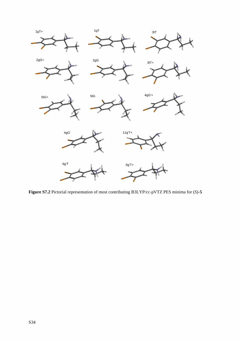
S34
1gT+ 1gT 3tT
2gG+ 2gG3tT+
5tG+ 5tG 4gG'+
4gG' 11g'T+
6g'T 6g'T+
Figure S7.2 Pictorial representation of most contributing B3LYP/cc-pVTZ PES minima for (S)-5

S35
Chapter 8
8.2 Intermolecular association of tetrahydrofuran-2-carboxylic acid in solution: A vibrational circular dichroism study Table S8.1 B3LYP/6-31++G** conformational description monomer 1 Table S8.2 B3LYP/ cc-pVTZ conformational description monomer 1 Table S8.3 B3LYP/ 6-31++G** conformational description dimer 1 Table S8.4 B3LYP/aug-cc-pVTZ monomer normal modes Table S8.5 B3LYP/aug-cc-pVTZ dimer normal modes Figure S8.1 The OH and CO stretching regions for solutions of (R)-(+)-1 in CS2
Figure S8.2 CDCl3 and CS2 simulated and experimental spectra Figure S8.3 Simulated IR DFT/6-31++G** spectra for different functionals Figure S8.4 Simulated VCD DFT/6-31++G** spectra for different functionals 8.4 A DFT conformational analysis and VCD study on methyl tetrahydrofuran-2-carboxylate Table S8.6 DFT/6-31G* conformational description 3 Table S8.7 DFT/cc-pVTZ fundamental assignment tables Figure S8.5 Simulated (S)-(+)-1 IR DFT/cc-pVTZ spectra for different functionals and experimental spectrum. Figure S8.6 Simulated (S)-(+)-1 VCD DFT/cc-pVTZ spectra for different functionals and experimental spectrum.

S36
Table S8.1 B3LYP/6-31++G** label, pseudo-rotational coordinates (q in Å and φ in degrees), key dihedral angles (τ1 and τ2 in degrees), relative free energies (ΔG0 in kcal/mol) and Boltzmann populations (% P, 298.15 K) for the unique monomer minima of 1. Minimum G and H are not reported.
label q φ τ1
O8C6C2O1 τ2
O7C6O8H9 ΔG0 % P
A 0.37 260 −3 182 0.00 38.79 B 0.36 77 5 180 0.09 33.25 C 0.35 108 152 −1 0.94 7.96 E 0.34 98 −30 −1 0.99 7.32 F 0.37 239 −39 −1 1.07 6.35 D 0.36 227 153 −1 1.07 6.32
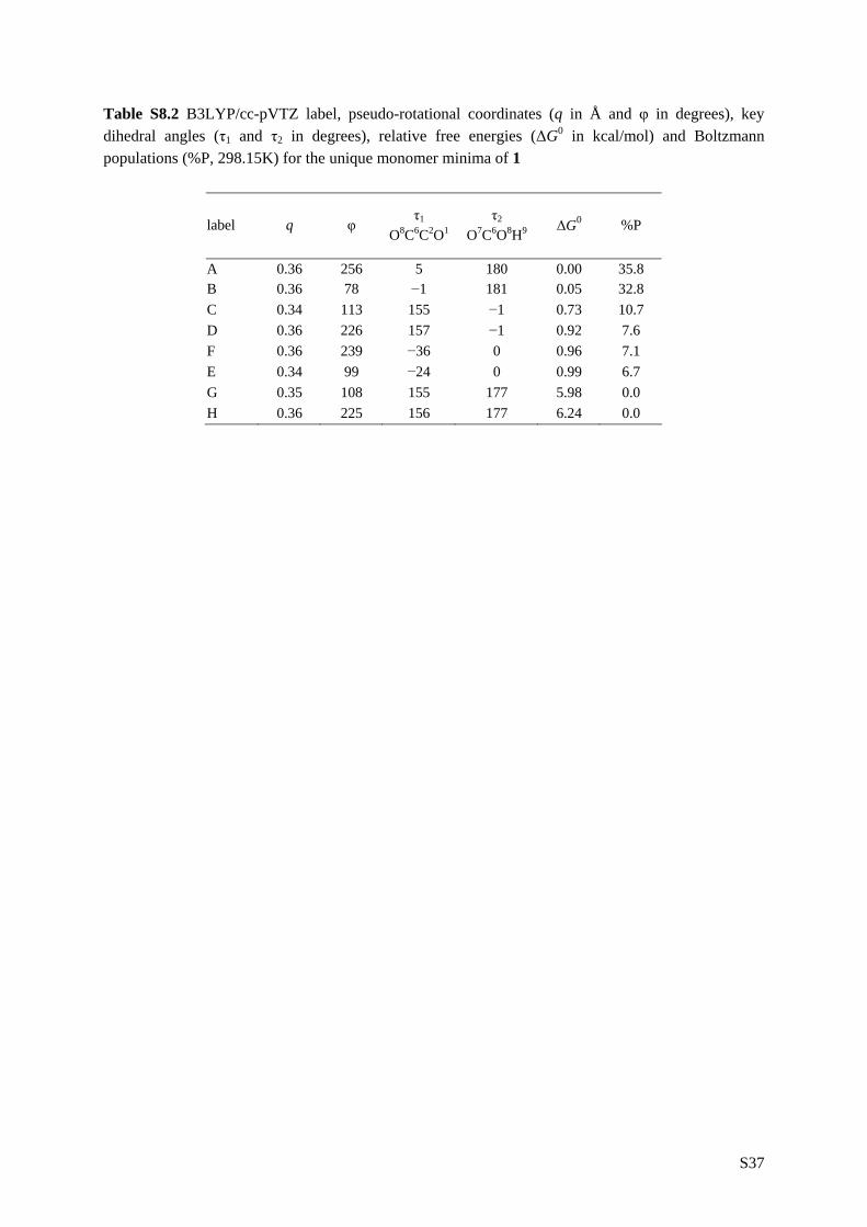
S37
Table S8.2 B3LYP/cc-pVTZ label, pseudo-rotational coordinates (q in Å and φ in degrees), key dihedral angles (τ1 and τ2 in degrees), relative free energies (ΔG0 in kcal/mol) and Boltzmann populations (%P, 298.15K) for the unique monomer minima of 1
label q φ τ1
O8C6C2O1τ2
O7C6O8H9 ΔG0 %P
A 0.36 256 5 180 0.00 35.8 B 0.36 78 −1 181 0.05 32.8 C 0.34 113 155 −1 0.73 10.7 D 0.36 226 157 −1 0.92 7.6 F 0.36 239 −36 0 0.96 7.1 E 0.34 99 −24 0 0.99 6.7 G 0.35 108 155 177 5.98 0.0 H 0.36 225 156 177 6.24 0.0
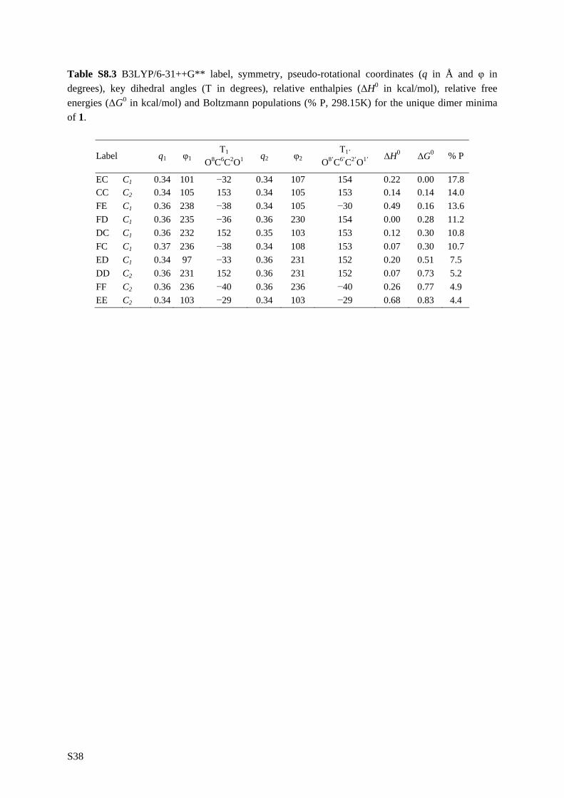
S38
Table S8.3 B3LYP/6-31++G** label, symmetry, pseudo-rotational coordinates (q in Å and φ in degrees), key dihedral angles (Τ in degrees), relative enthalpies (ΔH0 in kcal/mol), relative free energies (ΔG0 in kcal/mol) and Boltzmann populations (% P, 298.15K) for the unique dimer minima of 1.
Label q1 φ1 Τ1
O8C6C2O1 q2 φ2 Τ1’
O8’C6’C2’O1’ ΔH0 ΔG0 % P
EC C1 0.34 101 −32 0.34 107 154 0.22 0.00 17.8 CC C2 0.34 105 153 0.34 105 153 0.14 0.14 14.0 FE C1 0.36 238 −38 0.34 105 −30 0.49 0.16 13.6 FD C1 0.36 235 −36 0.36 230 154 0.00 0.28 11.2 DC C1 0.36 232 152 0.35 103 153 0.12 0.30 10.8 FC C1 0.37 236 −38 0.34 108 153 0.07 0.30 10.7 ED C1 0.34 97 −33 0.36 231 152 0.20 0.51 7.5 DD C2 0.36 231 152 0.36 231 152 0.07 0.73 5.2 FF C2 0.36 236 −40 0.36 236 −40 0.26 0.77 4.9 EE C2 0.34 103 −29 0.34 103 −29 0.68 0.83 4.4

S39S39
Table S8.4 B3LYP/aug-cc-pVTZ vibrational frequencies (ν, in cm−1), dipole strengths (D, in 10−40 esu2cm2) and rotational strengths (R, in 10−44 esu2cm2) for different (S)-monomer conformations.
A D E C B F ν D R ν D R ν D R ν D R ν D R ν D R
1 42 218 −13 46 204 −7 30 293 −14 42 156 −21 57 249 −16 37 154 −112 87 48 7 50 107 5 48 156 16 55 272 15 88 36 7 47 125 163 197 129 −1 191 8 3 158 5 3 152 16 5 198 100 3 195 11 24 239 151 −4 248 33 8 249 77 −13 241 7 0 285 210 −16 255 10 −25 317 177 29 300 11 5 288 11 −4 298 5 6 327 125 24 282 76 −46 443 21 0 410 78 −8 435 20 8 407 76 −6 474 20 3 425 17 57 561 30 −22 591 348 −18 578 149 −9 572 212 37 565 73 −57 583 322 318 612 53 −38 603 134 24 585 444 57 606 360 −111 589 6 6 597 195 109 678 28 4 640 253 −26 641 208 −13 641 145 47 678 41 1 628 392 −33
10 731 115 67 703 120 5 736 254 −33 738 218 13 752 350 0 691 63 1811 743 308 −23 751 152 0 755 98 47 757 95 12 756 98 25 757 211 2012 839 83 −49 812 31 3 819 4 −3 827 11 −5 822 7 5 818 34 −1813 881 63 46 874 39 20 869 40 8 869 16 2 882 79 −32 880 39 3214 906 29 −21 918 14 −14 900 43 4 906 12 12 907 60 10 911 44 −2815 934 9 9 930 17 4 924 45 −14 925 38 −6 929 31 −13 933 8 −116 940 87 −3 950 58 41 939 98 −27 939 88 −25 938 68 −45 943 84 7317 967 89 53 969 63 3 964 2 3 963 9 −8 968 29 −2 956 77 −1318 1039 94 6 1033 15 −13 1042 33 19 1040 17 7 1053 88 38 1029 40 119 1079 429 −21 1100 1148 −50 1101 310 −65 1101 1118 28 1074 438 75 1088 277 5120 1134 13 10 1112 318 −5 1108 353 79 1122 272 −22 1116 21 0 1123 288 −3321 1188 41 50 1151 121 2 1172 439 20 1141 244 −33 1180 106 −11 1182 566 −1722 1204 30 −32 1208 13 20 1197 57 20 1195 23 5 1193 16 −13 1205 26 2423 1214 6 −23 1213 24 27 1203 95 −45 1204 21 −1 1221 10 −35 1209 6 −924 1261 11 −7 1257 8 −4 1257 17 21 1255 8 9 1263 15 13 1261 12 −225 1304 21 7 1291 3 13 1287 6 16 1284 20 35 1292 6 6 1306 1 −226 1329 8 2 1315 17 −21 1324 3 5 1304 22 10 1329 5 −2 1336 3 −12

S40S40
27 1341 16 1 1330 14 19 1344 1 2 1325 3 3 1340 31 28 1338 4 328 1354 218 −85 1336 16 −16 1360 45 5 1347 4 2 1349 185 −70 1361 24 329 1375 621 65 1379 22 −5 1368 104 16 1389 22 −18 1375 581 122 1365 123 −2430 1394 314 4 1401 45 −6 1393 9 −4 1405 26 1 1397 336 −5 1387 10 −231 1493 12 −1 1492 8 −2 1496 15 −2 1495 11 −1 1495 13 −4 1492 7 −132 1503 12 −2 1506 11 −5 1505 18 −3 1504 16 −7 1505 21 −3 1503 14 −133 1529 1 3 1528 5 1 1531 1 −2 1530 2 2 1530 3 −6 1526 2 134 1836 727 −83 1820 607 17 1798 701 −58 1817 578 43 1835 687 −76 1800 745 −4935 3013 69 −7 3010 56 2 3021 86 5 3026 85 3 3016 73 7 3000 69 −436 3034 17 8 3052 29 −5 3054 20 6 3054 20 5 3047 20 5 3050 26 −1037 3047 16 −15 3060 22 10 3058 11 −14 3061 16 −16 3050 10 18 3056 21 1738 3056 24 3 3065 18 −6 3073 65 41 3075 59 45 3064 35 −14 3067 19 −1239 3090 39 −30 3096 22 −32 3076 4 0 3078 3 8 3093 30 25 3093 35 −4040 3104 30 26 3102 37 44 3102 24 −38 3101 14 −46 3105 34 −24 3101 31 4941 3125 16 −3 3117 36 −13 3115 31 23 3113 41 27 3127 8 7 3118 30 −1442 3614 173 −30 3734 71 4 3731 69 −4 3734 68 2 3605 181 −32 3737 74 −2

S41S41
Table S8.5 B3LYP/aug-cc-pVTZ vibrational frequencies (ν, in cm−1), dipole strengths (D, in 10−40 esu2cm2) and rotational strengths (R, in 10−44 esu2cm2) for different (SS)-dimer conformations.
CC FD DD EC EE DC FF ED FC FE
ν D R ν D R ν D R ν D R ν D R ν D R ν D R ν D R ν D R ν D R
1 18 7 −1 23 354 −3 24 112 −1 18 506 1 21 30 −2 10 31 2 15 67 −4 20 432 −2 19 443 1 18 20 −1
2 30 154 7 30 280 −2 34 215 7 29 299 1 34 119 −28 25 181 6 23 145 7 27 354 −11 27 81 2 27 149 8
3 37 237 −15 32 138 −5 34 18 5 39 45 3 35 107 7 41 145 −12 32 369 22 37 17 1 30 393 −17 37 57 −13
4 41 6 −1 46 185 20 40 91 0 44 190 −34 43 384 24 46 49 −4 39 88 −20 43 76 −3 42 249 −2 46 342 8
5 48 55 5 52 59 −11 47 57 −15 53 195 23 45 11 −2 50 62 4 40 17 −3 55 252 12 48 45 16 52 48 −1
6 71 110 −3 72 7 −2 72 112 1 71 4 1 73 40 6 73 108 −3 74 23 6 73 8 −1 73 6 −1 74 18 4
7 84 14 −1 85 25 0 85 9 0 86 25 −1 82 53 2 85 14 0 81 53 1 84 23 0 85 28 −1 82 52 2
8 110 858 −14 112 249 4 113 680 −4 112 260 0 117 26 7 112 745 −11 115 80 4 113 203 5 108 281 −3 117 29 5
9 120 2 4 134 98 4 125 0 2 136 106 −5 119 3 −2 125 3 3 122 0 0 135 112 2 137 98 3 122 16 0
10 144 1 1 142 2 −2 140 1 1 140 14 7 154 2 −3 142 17 1 152 1 −3 144 2 −1 140 7 3 153 2 −3
11 167 5 −6 211 4 3 211 5 2 164 71 −2 171 2 2 173 57 2 206 3 3 177 4 2 163 106 −3 169 3 2
12 168 127 11 223 106 8 222 139 4 178 6 1 171 3 3 217 73 4 217 34 14 218 63 5 216 19 6 218 18 9
13 260 5 1 258 31 4 265 75 8 261 42 0 265 4 3 262 54 4 266 30 −1 263 88 2 265 3 3 269 26 0
14 274 18 −1 273 1 −2 268 0 0 278 130 −3 277 235 −9 273 10 1 267 0 1 276 118 −10 271 14 −1 271 104 −2
15 333 1 −4 307 183 −14 330 1 −3 302 97 −13 312 2 8 332 8 −1 303 0 2 303 96 −10 307 178 −16 309 26 5
16 336 248 41 362 495 13 350 276 35 353 360 12 323 665 −38 345 245 34 328 855 −31 359 403 10 355 435 17 326 759 −34
17 434 0 0 428 27 −3 436 0 −2 432 25 −6 460 0 −6 436 4 −1 455 0 −1 428 23 −4 431 29 −5 457 47 −7
18 462 455 5 473 402 3 450 452 7 480 497 12 480 684 −6 457 440 6 464 602 −22 477 473 12 474 448 4 474 589 −12
19 596 0 0 595 5 4 597 4 −4 596 12 0 596 0 1 597 20 −5 591 5 0 594 10 −1 596 7 9 593 11 8
20 597 11 −9 598 23 1 598 29 −3 597 4 −4 597 22 1 598 2 −3 593 13 20 598 20 −2 601 6 −6 597 11 3
21 652 7 −19 674 30 13 676 1 10 652 14 22 645 8 5 654 109 −18 668 0 0 652 57 25 657 135 −9 649 43 20
22 660 351 −21 686 262 −26 690 478 −67 658 255 −24 656 165 49 683 319 −29 689 143 −9 684 285 −35 681 137 −13 681 118 6
23 729 85 −5 700 73 8 697 70 −11 730 83 −12 728 80 −5 701 39 −5 697 59 11 702 38 −6 700 96 15 697 108 23
24 733 30 −25 702 109 −16 701 37 5 736 17 −1 733 9 3 728 60 −18 701 184 36 732 47 −3 734 58 −13 731 49 0
25 772 11 8 748 34 −3 745 12 −6 772 1 7 771 6 1 748 6 2 748 29 0 749 10 5 752 14 −3 752 12 −1
26 782 123 52 752 5 3 753 24 13 779 109 27 781 76 −8 778 81 30 755 10 −4 773 44 2 777 73 34 777 55 −9
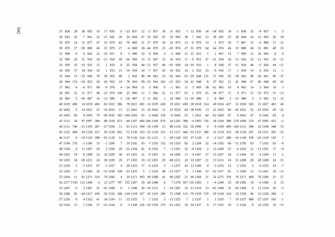
S42S42
27 838 29 38 835 16 17 835 9 −23 837 12 −2 837 18 31 835 7 12 836 18 −34 835 24 −1 838 32 −4 837 1 5
28 843 26 −7 841 32 −15 841 26 24 844 47 35 843 47 19 843 38 7 842 33 28 841 33 28 844 24 13 843 56 18
29 870 14 15 877 47 33 879 63 70 869 21 27 870 20 23 873 23 −6 879 14 −1 872 29 −7 867 12 −6 868 17 −12
30 870 27 −29 880 40 31 879 27 −4 869 18 −44 870 25 −45 876 47 31 879 64 64 876 46 31 880 40 31 881 40 33
31 908 0 0 916 22 −10 917 8 3 906 10 8 906 4 −2 909 15 15 915 1 1 907 12 7 909 15 16 906 8 8
32 909 29 31 919 18 −11 918 28 −26 909 15 15 907 15 16 919 17 −9 915 47 −21 918 18 −11 916 22 −11 916 25 −11
33 929 25 −33 932 15 2 933 8 25 928 40 −12 927 40 −41 930 34 −10 933 1 8 928 37 −11 929 40 −5 926 44 −11
34 929 37 18 934 10 1 933 21 −19 929 34 −7 927 45 19 932 16 2 933 25 −9 932 17 1 934 14 0 935 12 −1
35 944 13 −23 949 70 39 952 88 3 942 88 −38 943 23 −42 944 91 −29 948 131 37 945 92 −39 942 89 −26 941 96 −37
36 944 174 −34 953 50 43 953 19 78 943 99 −25 943 163 −31 953 54 41 948 8 47 952 51 41 948 67 40 948 69 42
37 965 4 −6 971 68 −9 976 4 −24 964 11 3 966 0 −1 965 11 3 969 38 −61 965 10 4 965 14 3 964 10 5
38 965 22 11 977 48 −12 979 140 25 966 11 5 966 22 11 977 63 1 970 65 34 977 71 0 971 51 −19 972 51 −13
39 983 5 −30 987 16 −13 990 5 −28 987 3 11 992 1 10 989 12 −19 980 1 6 989 3 −15 986 3 0 992 12 15
40 1019 490 10 1019 482 65 1022 386 78 1021 491 −14 1029 428 10 1021 459 28 1018 514 49 1024 437 52 1020 505 21 1027 403 40
41 1042 5 14 1031 47 −14 1033 11 15 1041 33 10 1042 12 21 1035 64 −38 1030 13 22 1035 84 −42 1032 52 −23 1032 95 −32
42 1043 83 0 1035 79 −49 1035 182 −104 1043 65 4 1044 136 −6 1042 55 1 1031 84 −62 1043 67 6 1042 47 6 1042 83 4
43 1111 18 97 1097 384 88 1104 673 −48 1107 404 168 1108 870 24 1105 384 −4 1093 745 18 1104 389 278 1096 374 47 1095 453 −2
44 1111 746 −23 1105 287 −27 1106 11 63 1111 384 −34 1109 13 88 1110 332 50 1096 0 −9 1106 400 −164 1111 346 32 1108 348 53
45 1125 460 −18 1128 227 93 1129 602 −73 1120 163 −25 1120 321 −32 1127 440 −52 1127 380 12 1119 153 −28 1126 207 14 1121 203 −25
46 1127 0 −10 1129 288 −91 1129 14 78 1126 224 −25 1122 3 −28 1128 105 37 1128 0 −2 1127 288 −10 1128 199 −25 1129 159 7
47 1194 170 −3 1206 15 −1 1206 7 19 1192 93 −7 1193 152 −10 1193 82 2 1204 32 −14 1192 68 −11 1195 93 7 1192 83 −4
48 1194 4 11 1207 20 1 1206 29 −22 1194 81 8 1193 7 −1 1201 32 −8 1204 2 13 1200 25 −4 1203 21 −13 1201 17 −9
49 1202 19 8 1208 23 32 1209 30 43 1201 21 −9 1201 11 34 1206 17 −4 1207 27 53 1207 18 −3 1206 19 4 1206 17 2
50 1203 34 −29 1211 24 30 1209 20 17 1202 19 −12 1201 29 −48 1211 22 33 1207 21 13 1211 24 31 1208 20 28 1208 24 31
51 1256 2 −1 1257 67 −1 1257 4 29 1253 17 −4 1254 3 −1 1257 42 13 1260 0 −3 1255 12 −3 1255 5 0 1252 24 −7
52 1256 17 9 1260 16 −12 1258 108 −33 1255 5 2 1254 48 −12 1257 9 1 1260 33 −22 1257 81 −5 1260 12 −6 1261 16 −13
53 1264 11 81 1271 314 76 1266 4 24 1271 493 69 1288 41 46 1265 21 46 1304 11 32 1271 329 76 1271 469 76 1286 21 27
54 1277 1139 112 1306 6 12 1277 797 155 1287 24 44 1288 4 7 1276 957 135 1305 1 −4 1290 33 30 1285 19 −6 1306 6 13
55 1287 0 3 1307 31 −41 1308 0 1 1288 20 −10 1315 1 −18 1287 35 −11 1319 13 −65 1308 32 −45 1306 6 12 1316 50 −2
56 1288 95 −44 1327 439 −20 1310 206 −134 1318 227 45 1319 299 75 1308 115 −76 1329 570 29 1318 224 33 1326 40 23 1326 266 −1
57 1326 0 4 1332 41 34 1334 11 32 1325 7 2 1335 3 −15 1325 7 2 1337 1 1 1333 7 19 1327 406 −27 1337 183 −1
58 1326 15 1 1336 37 −33 1334 0 3 1338 226 −29 1339 373 −55 1332 20 24 1337 9 17 1335 10 −2 1336 8 10 1339 10 −15
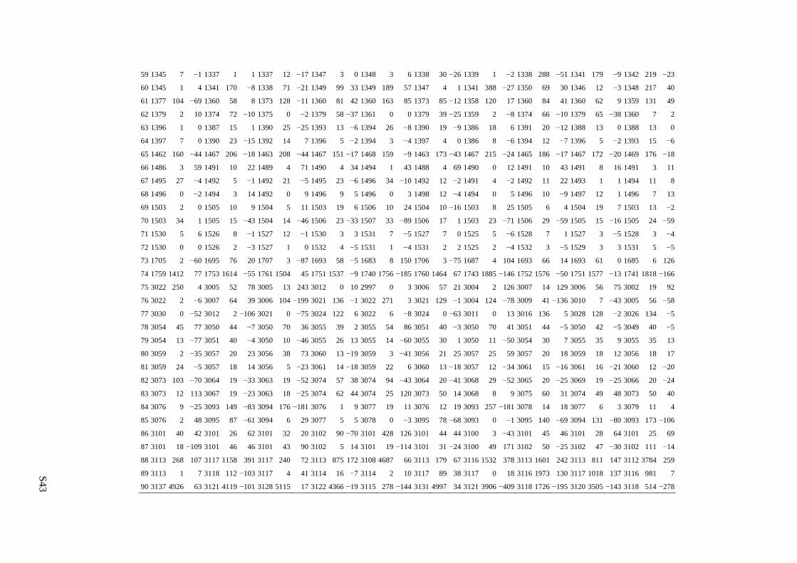
S43S43
59 1345 7 −1 1337 1 1 1337 12 −17 1347 3 0 1348 3 6 1338 30 −26 1339 1 −2 1338 288 −51 1341 179 −9 1342 219 −23
60 1345 1 4 1341 170 −8 1338 71 −21 1349 99 33 1349 189 57 1347 4 1 1341 388 −27 1350 69 30 1346 12 −3 1348 217 40
61 1377 104 −69 1360 58 8 1373 128 −11 1360 81 42 1360 163 85 1373 85 −12 1358 120 17 1360 84 41 1360 62 9 1359 131 49
62 1379 2 10 1374 72 −10 1375 0 −2 1379 58 −37 1361 0 0 1379 39 −25 1359 2 −8 1374 66 −10 1379 65 −38 1360 7 2
63 1396 1 0 1387 15 1 1390 25 −25 1393 13 −6 1394 26 −8 1390 19 −9 1386 18 6 1391 20 −12 1388 13 0 1388 13 0
64 1397 7 0 1390 23 −15 1392 14 7 1396 5 −2 1394 3 −4 1397 4 0 1386 8 −6 1394 12 −7 1396 5 −2 1393 15 −6
65 1462 160 −44 1467 206 −18 1463 208 −44 1467 151 −17 1468 159 −9 1463 173 −43 1467 215 −24 1465 186 −17 1467 172 −20 1469 176 −18
66 1486 3 59 1491 10 22 1489 4 71 1490 4 34 1494 1 43 1488 4 69 1490 0 12 1491 10 43 1491 8 16 1491 3 11
67 1495 27 −4 1492 5 −1 1492 21 −5 1495 23 −6 1496 34 −10 1492 12 −2 1491 4 −2 1492 11 22 1493 1 1 1494 11 8
68 1496 0 −2 1494 3 14 1492 0 9 1496 9 5 1496 0 3 1498 12 −4 1494 0 5 1496 10 −9 1497 12 1 1496 7 13
69 1503 2 0 1505 10 9 1504 5 11 1503 19 6 1506 10 24 1504 10 −16 1503 8 25 1505 6 4 1504 19 7 1503 13 −2
70 1503 34 1 1505 15 −43 1504 14 −46 1506 23 −33 1507 33 −89 1506 17 1 1503 23 −71 1506 29 −59 1505 15 −16 1505 24 −59
71 1530 5 6 1526 8 −1 1527 12 −1 1530 3 3 1531 7 −5 1527 7 0 1525 5 −6 1528 7 1 1527 3 −5 1528 3 −4
72 1530 0 0 1526 2 −3 1527 1 0 1532 4 −5 1531 1 −4 1531 2 2 1525 2 −4 1532 3 −5 1529 3 3 1531 5 −5
73 1705 2 −60 1695 76 20 1707 3 −87 1693 58 −5 1683 8 150 1706 3 −75 1687 4 104 1693 66 14 1693 61 0 1685 6 126
74 1759 1412 77 1753 1614 −55 1761 1504 45 1751 1537 −9 1740 1756 −185 1760 1464 67 1743 1885 −146 1752 1576 −50 1751 1577 −13 1741 1818 −166
75 3022 250 4 3005 52 78 3005 13 243 3012 0 10 2997 0 3 3006 57 21 3004 2 126 3007 14 129 3006 56 75 3002 19 92
76 3022 2 −6 3007 64 39 3006 104 −199 3021 136 −1 3022 271 3 3021 129 −1 3004 124 −78 3009 41 −136 3010 7 −43 3005 56 −58
77 3030 0 −52 3012 2 −106 3021 0 −75 3024 122 6 3022 6 −8 3024 0 −63 3011 0 13 3016 136 5 3028 128 −2 3026 134 −5
78 3054 45 77 3050 44 −7 3050 70 36 3055 39 2 3055 54 86 3051 40 −3 3050 70 41 3051 44 −5 3050 42 −5 3049 40 −5
79 3054 13 −77 3051 40 −4 3050 10 −46 3055 26 13 3055 14 −60 3055 30 1 3050 11 −50 3054 30 7 3055 35 9 3055 35 13
80 3059 2 −35 3057 20 23 3056 38 73 3060 13 −19 3059 3 −41 3056 21 25 3057 25 59 3057 20 18 3059 18 12 3056 18 17
81 3059 24 −5 3057 18 14 3056 5 −23 3061 14 −18 3059 22 6 3060 13 −18 3057 12 −34 3061 15 −16 3061 16 −21 3060 12 −20
82 3073 103 −70 3064 19 −33 3063 19 −52 3074 57 38 3074 94 −43 3064 20 −41 3068 29 −52 3065 20 −25 3069 19 −25 3066 20 −24
83 3073 12 113 3067 19 −23 3063 18 −25 3074 62 44 3074 25 120 3073 50 14 3068 8 9 3075 60 31 3074 49 48 3073 50 40
84 3076 9 −25 3093 149 −83 3094 176 −181 3076 1 9 3077 19 11 3076 12 19 3093 257 −181 3078 14 18 3077 6 3 3079 11 4
85 3076 2 48 3095 87 −61 3094 6 29 3077 5 5 3078 0 −3 3095 78 −68 3093 0 −1 3095 140 −69 3094 131 −80 3093 173 −106
86 3101 40 42 3101 26 62 3101 32 20 3102 90 −70 3101 428 126 3101 44 44 3100 3 −43 3101 45 46 3101 28 64 3101 25 69
87 3101 18 −109 3101 46 46 3101 43 90 3102 5 14 3101 19 −114 3101 31 −24 3100 49 171 3102 50 −25 3102 47 −30 3102 111 −14
88 3113 268 107 3117 1158 391 3117 240 72 3113 875 172 3108 4687 66 3113 179 67 3116 1532 378 3113 1601 242 3113 811 147 3112 3784 259
89 3113 1 7 3118 112 −103 3117 4 41 3114 16 −7 3114 2 10 3117 89 38 3117 0 18 3116 1973 130 3117 1018 137 3116 981 7
90 3137 4926 63 3121 4119 −101 3128 5115 17 3122 4366 −19 3115 278 −144 3131 4997 34 3121 3906 −409 3118 1726 −195 3120 3505 −143 3118 514 −278
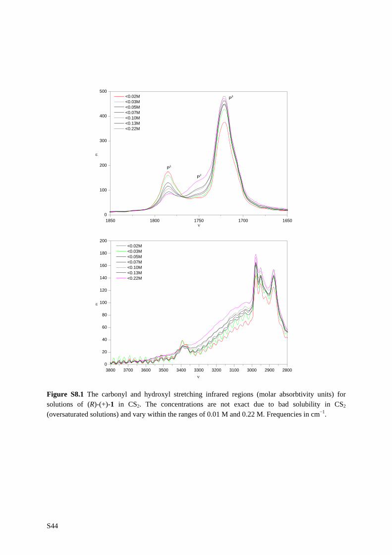
S44
1850 1800 1750 1700 16500
100
200
300
400
500 <0.02M <0.03M <0.05M <0.07M <0.10M <0.13M <0.22M
P3
P2
P1
ν
ε
3800 3700 3600 3500 3400 3300 3200 3100 3000 2900 28000
20
40
60
80
100
120
140
160
180
200 <0.02M <0.03M <0.05M <0.07M <0.10M <0.13M <0.22M
ν
ε
Figure S8.1 The carbonyl and hydroxyl stretching infrared regions (molar absorbtivity units) for solutions of (R)-(+)-1 in CS2. The concentrations are not exact due to bad solubility in CS2 (oversaturated solutions) and vary within the ranges of 0.01 M and 0.22 M. Frequencies in cm−1.

S45
1800 1600 1400 1200 1000 800050100150200250300350400450500550600
-0.01
0.00
0.01
(ii)
Δ ε
fm1
=0.40, fm2
=0.25 and fd=0.35
fm1=0.35, fm2=0.10 and fd=0.55
ν
Δ ε
ε
(i)
1850 1800 1750 1700 1650 16000
100
200
300
400
ε
-0.01
0.00
0.01
0.42M CDCl3
x0.25
x0.25
0.11M CS2
Figure S8.2 (i) B3LYP/aug-cc-pVTZ simulated spectra for different fraction of monomer and dimer; black spectra:
1mf = 0.40, 2mf = 0.25 and df = 0.35, and
1mf = 0.35, 2mf = 0.10, df = 0.55 based on an
“educated guess” for CS2 equilibrium fractions (there are indications for monomer solvent-solute stabilization in CDCl3; the fraction of dimer in CS2 is larger, the fraction of monomer 1 (A/B) only slightly lower, due to the extra stabilization of the intra-molecular hydrogen bond, and for monomer 2 (C/D/E/F) the fraction is low). (ii) Experimental spectra for (S)-(−)-1 in CDCl3 (0.42M) and CS2 (0.11M) scaled down (factor 0.25). Intensities in molar absorptivity units, frequencies is cm−1

S46
1800 1700 1600 1500 1400 1300 1200 1100 1000 900 8000
50100150200250300
ν
1800 1700 1600 1500 1400 1300 1200 1100 1000 900 800
B3LYP
B3PW91
B3P86
B1LYP
MPW1PW91
B98
PBE1PBE
ε
Figure S8.3 Simulated IR DFT/6-31++G** spectra for different functionals. Intensities are in molar absorptivity units, frequencies in cm−1

S47
1800 1700 1600 1500 1400 1300 1200 1100 1000 900 800-0.015-0.010-0.0050.0000.0050.0100.015
ν
B3LYP
B3PW91
B3P86
B1LYP
MPW1PW91
Δ ε
B98
1800 1700 1600 1500 1400 1300 1200 1100 1000 900 800
PBE1PBE
Figure S8.4 Simulated VCD DFT/6-31++G** spectra for different functionals. Intensities are in molar absorptivity units, frequencies in cm−1

S48
Table S8.6 DFT (B1LYP, B3LYP, B3P86, B3PW91, B98, BHandH, BHandHLYP, MPW1PW91 and PBE1PBE)/6-31G* label, pseudo-rotational coordinates (q in Å and φ in degrees), key dihedral angle (τ1 in degrees), relative Gibbs energies (ΔG0 in kcal/mol) and Boltzmann populations (% P, 298.15 K) for located conformations of 3.
functional conf τ1
O8C6C2O1 q φ ΔG0
% P B1LYP U 147 0.37 226 0.00 28.24 Y 111 0.37 228 0.01 27.69 T 153 0.36 113 0.14 22.46 X −25 0.35 103 0.51 11.96 V −44 0.37 237 0.64 9.64 B3LYP T 152 0.36 112 0.00 34.43 Y 109 0.38 228 0.03 32.71 X −24 0.35 103 0.38 18.23 V −43 0.37 237 0.51 14.63 B3P86 T 154 0.36 113 0.00 27.28 U 151 0.38 224 0.04 25.69 Y 107 0.38 227 0.17 20.54 X −19 0.36 105 0.34 15.37 V −40 0.37 237 0.53 11.12 B3PW91 Y 112 0.38 229 0.00 38.30 U 150 0.37 226 0.36 20.98 T 154 0.36 112 0.38 20.33 X −19 0.36 103 0.72 11.44 V −40 0.37 238 0.86 8.96 B98 T 155 0.36 116 0.00 34.03 U 152 0.37 222 0.03 32.27 X −21 0.36 108 0.36 18.40 V −42 0.37 235 0.47 15.31 BHandH T 159 0.37 117 0.00 36.93 X −18 0.37 111 0.30 22.35 U 164 0.38 215 0.62 12.87 V −39 0.38 233 0.79 9.82 Y 104 0.39 224 0.81 9.40 W 73 0.38 84 0.86 8.64 BHandHLYP T 156 0.35 113 0.00 33.55 U 157 0.36 223 0.29 20.61 X −25 0.35 104 0.33 19.13 V −42 0.37 238 0.53 13.65 W 83 0.36 83 0.56 13.06 MPW1PW91 T 155 0.36 114 0.00 35.86 U 154 0.37 224 0.15 28.07 X −19 0.36 105 0.31 21.26 V −40 0.37 237 0.52 14.81 PBE1PBE Y 111 0.38 227 0.00 34.05 T 156 0.36 114 0.20 24.15

S49
U 155 0.38 222 0.38 17.79 X −18 0.37 107 0.51 14.36 V −39 0.38 236 0.75 9.66

S50
Table S8.7 Lorentzian fitted experimental and broadened DFT (B3LYP, B3LYP, B3P86, B3PW91, B98, BHandHLYP, MPW1PW91 and PBE1PBE)/cc-pVTZ IR/VCD frequencies (υ, in cm−1) and dipole/rotational strengths (D in 10−40 esu2cm2 and R in 10−44 esu2cm2) accounting for the significant minima i.e. T, U, X, V and W. Harmonic frequencies are scaled with factor 0.98.
B3LYP/cc-pVTZ experiment
Fund v D R v D fund v R fund
21U 1015.4 5.3 −2.3 1039.0 65.1 21
21T 1020.5 4.8 3.0 1035.4 9.4 21TXV
21X 1024.3 12.3 3.4 1045.0 3.8
21V 1026.3 39.4 0.0 1054.4 0.4
21W 1045.5 6.1 2.2 1074.0 81.1 21W/22/23 1067.8 2.9 21W/22/23X
22W 1057.5 81.4 8.9 1086.6 266.4 1075.4 7.7
22V 1069.7 72.3 9.8 1097.3 193.5 1081.1 7.3
22U 1083.1 111.6 10.0 1108.9 18.0 1085.9 14.0
22X 1085.3 70.4 9.7
22T 1088.2 106.7 11.9
23X 1093.4 35.4 −5.2
23W 1098.5 2.9 −2.4 1098.4 2.2 23
23T 1102.4 103.9 1.3 1101.1 2.6
23U 1103.5 125.5 0.9
23V 1107.6 20.0 −2.6
24W 1151.5 0.9 0.5 1176.1 135.5 24/25/26WXT 1163.9 −3.8 24/25/26WXT
24T 1151.9 1.2 −0.8 1177.2 −19.7
24U 1152.0 1.5 −1.1
24X 1152.1 0.7 0.0
24V 1152.3 0.6 0.1
25X 1163.6 23.5 −0.9
25T 1164.5 152.8 6.9
25W 1168.1 23.6 −2.2
25U 1171.3 120.5 −4.7
26W 1172.2 35.2 −3.7
26X 1173.1 3.1 −0.9
26T 1174.6 9.2 −2.8
25V 1180.7 7.8 3.7 1213.6 498.2 25V/26VU/27/28/29 1191.1 2.9 25V/26VU/27/28TUW
26V 1181.0 1.7 2.7 1255.5 77.0 1210.9 31.4
27T 1183.4 7.4 0.6 1218.5 6.8
26U 1184.2 4.4 2.4
27W 1185.7 1.8 −0.3
27X 1186.2 7.8 0.3
27V 1187.1 4.4 1.0
27U 1187.2 21.3 10.5
28T 1192.5 168.1 4.0
28U 1196.9 119.8 14.1
28W 1204.5 108.1 4.9
28X 1223.1 24.6 −6.4 1238.7 1.3 28XV/29/30TX
29T 1228.8 4.2 3.3 1245.6 −1.1
29U 1233.1 0.3 −1.3 1259.1 −1.6
28V 1235.5 4.8 −3.7 1261.2 2.4
29W 1237.2 6.2 3.5
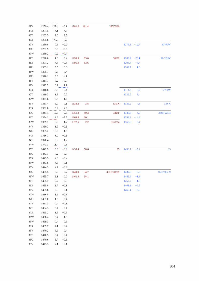
S51
29V 1259.4 127.4 −8.1 1281.2 111.4 29VX/30
29X 1261.5 14.1 4.6
30T 1263.5 2.0 2.5
30X 1265.8 76.8 3.7
30V 1280.8 0.9 −2.2 1275.8 −12.7 30VUW
30U 1281.9 8.0 −10.8
30W 1289.2 0.2 −0.7
31T 1298.0 1.0 0.4 1293.3 63.0 31/32 1283.9 −20.1 31/32UV
31X 1301.2 4.8 −2.8 1305.0 13.6 1293.8 −6.4
31U 1303.1 5.5 3.3 1302.7 −1.8
31W 1305.7 0.9 0.4
32U 1310.1 3.8 −4.1
31V 1311.7 3.2 −0.7
32V 1312.2 0.2 1.1
32X 1318.8 3.0 2.4 1314.3 6.7 32XTW
32T 1319.3 1.3 0.0 1322.6 3.4
32W 1321.6 0.5 −1.0
33V 1331.4 5.0 0.1 1338.2 3.8 33VX 1335.2 7.8 33VX
33X 1331.8 5.9 4.6
33U 1347.4 12.5 −2.5 1351.8 40.3 33UT 1346.6 −4.3 33UTW/34
33T 1354.1 13.6 −7.5 1369.8 20.1 1352.3 −14.3
33W 1359.1 0.9 1.2 1377.5 2.2 33W/34 1368.6 −6.4
34V 1360.2 1.2 −0.3
34U 1365.2 10.5 −1.5
34X 1366.2 1.0 −0.5
34T 1370.4 3.9 1.2
34W 1371.3 11.4 0.6
35T 1442.9 6.6 −0.8 1438.4 58.6 35 1436.7 −5.2 35
35U 1443.1 7.2 −0.7
35X 1443.5 4.0 −0.4
35W 1443.8 4.3 −0.1
35V 1444.3 4.7 −0.3
36U 1455.5 5.9 0.2 1449.9 34.7 36/37/38/39 1437.6 −5.9 36/37/38/39
36W 1455.7 3.1 0.0 1461.3 38.1 1442.9 −1.8
36T 1455.7 6.2 0.3 1452.2 −1.9
36X 1455.8 3.7 −0.1 1461.8 −2.5
36V 1455.8 3.6 −0.1 1465.4 −0.3
37W 1456.5 1.9 −0.5
37U 1461.0 1.9 −0.4
37V 1461.3 0.7 −0.1
37T 1464.3 3.4 −0.4
37X 1465.2 1.9 −0.5
38W 1468.4 6.7 −1.3
39W 1469.3 0.4 0.6
38X 1469.7 4.1 0.4
38V 1470.2 3.6 0.4
38T 1470.5 6.7 −0.7
38U 1470.6 6.7 −0.6
39V 1473.3 2.1 0.1
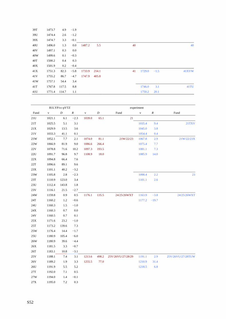
S52
39T 1473.7 4.9 −1.9
39U 1474.4 2.6 −1.2
39X 1474.7 3.3 −0.1
40U 1496.0 1.3 0.0 1487.2 5.5 40 40
40V 1497.1 0.3 0.0
40W 1499.6 0.1 −0.3
40T 1500.2 0.4 0.3
40X 1501.9 0.2 −0.4
41X 1751.3 82.3 −5.8 1733.9 214.1 41 1729.0 −1.5 41XVW
41V 1755.2 86.7 −4.7 1747.9 405.8
41W 1757.1 54.4 3.4
41T 1767.8 117.5 8.8 1746.0 3.1 41TU
41U 1771.4 114.7 1.1 1750.2 20.1
B1LYP/cc-pVTZ experiment
Fund v D R v D Fund v R Fund
21U 1021.1 6.1 −2.3 1039.0 65.1 21
21T 1025.5 5.1 3.1 1035.4 9.4 21TXV
21X 1029.9 13.5 3.6 1045.0 3.8
21V 1033.3 41.1 0.1 1054.4 0.4
21W 1052.1 7.7 2.1 1074.0 81.1 21W/22/23 1067.8 2.9 21W/22/23X
22W 1066.9 81.9 9.0 1086.6 266.4 1075.4 7.7
22V 1078.8 71.6 10.2 1097.3 193.5 1081.1 7.3
22U 1091.7 96.8 9.7 1108.9 18.0 1085.9 14.0
22X 1094.8 66.4 7.6
22T 1096.6 89.1 9.6
23X 1101.1 40.2 −3.2
23W 1105.8 2.8 −2.3 1098.4 2.2 23
23T 1110.9 123.0 3.4 1101.1 2.6
23U 1112.4 143.8 1.8
23V 1116.1 21.5 −2.7
24W 1159.8 0.9 0.5 1176.1 135.5 24/25/26WXT 1163.9 −3.8 24/25/26WXT
24T 1160.2 1.2 −0.6 1177.2 −19.7
24U 1160.3 1.5 −1.0
24X 1160.3 0.7 0.0
24V 1160.5 0.7 0.1
25X 1171.6 23.2 −1.0
25T 1173.2 139.6 7.3
25W 1176.4 14.4 −1.7
25U 1180.9 105.4 −6.0
26W 1180.9 39.6 −4.4
26X 1181.5 3.3 −0.7
26T 1183.1 10.8 −3.1
25V 1188.1 7.4 3.1 1213.6 498.2 25V/26VU/27/28/29 1191.1 2.9 25V/26VU/27/28TUW
26V 1189.2 1.9 3.3 1255.5 77.0 1210.9 31.4
26U 1191.9 5.5 5.2 1218.5 6.8
27T 1192.0 7.1 0.5
27W 1194.0 1.4 −0.1
27X 1195.0 7.2 0.3

S53
27V 1195.7 4.1 1.0
27U 1195.7 17.4 8.6
28T 1203.0 185.6 4.8
28U 1206.6 139.9 14.9
28W 1215.3 115.6 4.8
28X 1231.7 22.2 −6.1 1238.7 1.3 28XV/29/30TX
29T 1236.7 4.1 3.3 1245.6 −1.1
29U 1240.9 0.3 −1.3 1259.1 −1.6
28V 1243.7 3.9 −3.3 1261.2 2.4
29W 1245.2 6.4 3.6
29V 1270.7 131.2 −8.5 1281.2 111.4 29VX/30
29X 1271.5 7.8 3.9
30T 1272.7 1.9 2.3
30X 1276.5 88.2 3.8
30V 1290.1 1.2 −2.4 1275.8 −12.7 30VUW
30U 1290.9 8.4 −11.0
30W 1298.2 0.2 −0.7
31T 1307.2 1.0 0.4 1293.3 63.0 31/32 1283.9 −20.1 31/32UV
31X 1310.5 5.5 −2.9 1305.0 13.6 1293.8 −6.4
31U 1311.9 5.9 2.7 1302.7 −1.8
31W 1315.1 0.9 0.5
32U 1319.2 3.5 −3.7
31V 1320.5 3.4 −0.9
32V 1322.2 0.4 1.3
32X 1327.9 3.2 2.5 1314.3 6.7 32XTW
32T 1328.1 1.3 0.1 1322.6 3.4
32W 1330.4 0.5 −1.0
33V 1341.2 5.1 0.2 1338.2 3.8 33VX 1335.2 7.8 33VX
33X 1341.3 6.2 4.7
33U 1357.3 12.6 −2.8 1351.8 40.3 33UT 1346.6 −4.3 33UTW/34
33T 1364.2 14.1 −7.9 1352.3 −14.3
33W 1369.1 0.8 1.2 1369.8 20.1 33W/34 1368.6 −6.4
34V 1370.2 1.3 −0.3 1377.5 2.2
34U 1376.0 11.1 −1.7
34X 1376.2 1.1 −0.5
34T 1380.9 4.6 1.1
34W 1382.3 12.1 0.7
35T 1453.6 6.5 −0.8 1438.4 58.6 35 1436.7 −5.2 35
35U 1453.8 7.1 −0.7
35X 1454.1 3.9 −0.4
35W 1454.7 4.3 −0.1
35V 1454.9 4.6 −0.3
36U 1465.4 5.7 0.2 1449.9 34.7 36/37/38/39 1437.6 −5.9 36/37/38/39
36T 1465.6 6.0 0.3 1461.3 38.1 1442.9 −1.8
36W 1465.6 3.0 0.0 1452.2 −1.9
36X 1465.7 3.6 −0.1 1461.8 −2.5
36V 1465.7 3.5 −0.1 1465.4 −0.3
37W 1466.2 1.8 −0.5
37U 1470.6 1.8 −0.4
37V 1470.9 0.7 −0.1

S54
37T 1473.9 3.3 −0.4
37X 1474.8 1.8 −0.5
38W 1478.2 6.6 −1.1
39W 1479.1 0.3 0.4
38X 1479.4 4.1 0.4
38V 1479.9 3.6 0.4
38T 1480.1 6.6 −0.6
38U 1480.3 6.6 −0.6
39V 1483.0 2.0 0.0
39T 1483.5 4.7 −1.8
39U 1484.3 2.5 −1.2
39X 1484.5 3.2 −0.1
40U 1506.2 1.2 0.0 1487.2 5.5 40 40
40V 1507.1 0.3 0.0
40W 1509.5 0.1 −0.3
40T 1510.2 0.4 0.3
40X 1511.8 0.2 −0.4
41X 1762.8 83.9 −5.8 1733.9 214.1 41 1729.0 −1.5 41XVW
41V 1766.9 88.1 −4.7 1747.9 405.8
41W 1768.5 55.4 3.3
41T 1779.4 119.6 9.0 1746.0 3.1 41TU
41U 1783.1 117.0 1.3 1750.2 20.1
B3P86/cc-pVTZ experiment
Fund v D R v D Fund v R Fund
21U 1030.0 11.1 −5.1 1039.0 65.1 21
21T 1031.8 5.4 3.6
21X 1039.6 16.0 3.1 1035.4 9.4 21XVW
21V 1049.8 33.4 −0.6 1045.0 3.8
21W 1057.0 6.1 1.1 1054.4 0.4
22W 1082.6 58.7 5.7 1074.0 81.1 22/23 1067.8 2.9 22/23W
22U 1086.5 14.9 4.5 1086.6 266.4 1075.4 7.7
22V 1086.5 47.8 8.5 1097.3 193.5 1081.1 7.3
22T 1091.7 8.1 −3.0 1108.9 18.0 1085.9 14.0
22X 1093.5 23.1 −10.7
23W 1095.8 5.1 −0.9
23X 1112.5 84.6 14.8 1098.4 2.2 23XVTU
23V 1118.7 45.4 0.2 1101.1 2.6
23T 1121.8 180.3 8.9
23U 1124.7 192.5 5.6
24W 1150.9 0.6 0.4 1176.1 135.5 24/25XWTU/26XWT 1163.9 −3.8 24
24T 1151.4 0.8 −0.4
24U 1151.5 0.9 −0.6
24X 1151.6 0.6 0.0
24V 1151.7 0.5 0.1
25X 1164.8 24.3 0.8 1177.2 −19.7 25XWTU/26XWT
25W 1168.5 1.2 −0.4
25T 1168.6 98.4 9.1
26X 1173.3 4.9 −1.2

S55
26W 1175.2 19.4 −2.8
26T 1175.6 4.9 −4.0
25U 1176.6 28.0 −6.2
25V 1180.0 4.3 0.4 1213.6 498.2 25V/26VU/27/28/29TUW 1191.1 2.9 25V/26VU/27/28TUW
26V 1181.9 2.1 3.2 1255.5 77.0 1210.9 31.4
26U 1183.5 5.2 −2.1 1218.5 6.8
27T 1184.4 4.7 1.9
27X 1185.5 11.1 0.3
27V 1187.7 6.7 3.2
27W 1187.9 6.5 −1.7
27U 1189.9 23.0 14.2
28T 1206.5 248.2 11.0
28U 1208.8 168.0 21.3
28W 1219.8 95.6 3.0
28X 1226.0 14.1 −4.5 1238.7 1.3 28XV/29TUWX/30T
29T 1228.6 8.6 5.5 1245.6 −1.1
29U 1232.2 1.4 −0.9 1259.1 −1.6
28V 1235.8 2.1 −1.9 1261.2 2.4
29W 1238.0 10.8 4.3
29X 1259.2 1.3 3.3 1281.2 111.4 29XV/30/31/32
30T 1262.9 2.6 1.1 1293.3 63.0
29V 1271.2 17.1 5.7 1305.0 13.6 1275.8 −12.7 29V/30UXVW/31/32UV
30U 1276.6 12.5 −13.7 1283.9 −20.1
30X 1280.5 77.3 6.7 1293.8 −6.4
30V 1284.4 107.5 −18.0 1302.7 −1.8
30W 1286.2 0.5 −1.5
31T 1289.5 1.5 0.4
31X 1296.2 35.9 −10.5
31U 1297.3 5.2 4.9
31W 1301.1 1.1 0.7
32U 1305.2 7.5 −6.3
31V 1306.0 1.6 −0.8
32V 1308.9 9.6 1.6
32X 1315.6 6.1 3.2 1314.3 6.7 32XTW
32T 1316.8 1.8 0.4 1322.6 3.4
32W 1317.8 0.5 −0.8
33V 1327.1 3.3 −0.1 1338.2 3.8 33VX 1335.2 7.8 33VX
33X 1328.1 9.5 7.9
33U 1345.5 16.0 −1.9 1351.8 40.3 33UTW/34V 1346.6 −4.3 33UTW/34
33T 1353.2 21.2 −9.9 1352.3 −14.3
33W 1356.7 0.3 0.6 1368.6 −6.4
34V 1357.7 1.4 −0.2
34X 1364.8 1.5 −0.3 1369.8 20.1 34XUZW
34U 1365.8 15.1 −3.0 1377.5 2.2
34T 1371.6 7.4 0.4
34W 1374.2 13.5 1.2
35T 1438.2 12.5 −1.6 1438.4 58.6 35 1436.7 −5.2 35
35U 1438.4 12.0 −1.1
35X 1438.6 7.8 −0.6
35V 1439.5 8.5 −0.6

S56
35W 1440.2 7.0 −0.1
36W 1444.5 1.8 −0.5 1449.9 34.7 36/37/38/39 1437.6 −5.9 36/37/38/39
36U 1448.3 6.2 0.1 1461.3 38.1 1442.9 −1.8
36X 1448.5 4.6 0.0 1452.2 −1.9
36T 1448.5 7.4 0.4 1461.8 −2.5
36V 1448.6 4.1 −0.1 1465.4 −0.3
37W 1448.6 3.0 0.0
37V 1450.8 0.8 −0.1
37U 1450.8 2.6 −0.4
37T 1453.4 4.8 −0.5
37X 1454.4 2.8 −0.9
38W 1458.6 3.8 −1.1
39W 1462.7 2.3 0.4
38X 1463.4 4.5 0.7
38T 1463.7 6.8 −3.0
38V 1463.8 1.9 −1.4
39V 1464.0 4.6 2.0
39T 1464.3 7.4 −0.1
38U 1464.5 6.9 −0.2
39X 1465.0 4.6 −0.1
39U 1465.8 3.1 −1.9
40U 1487.9 1.5 −0.1 1487.2 5.5 40 40
40V 1489.3 0.4 0.0
40W 1492.6 0.0 −0.2
40T 1493.1 0.7 0.5
40X 1495.0 0.4 −0.4
41X 1773.0 88.5 −6.7 1733.9 214.1 41 1729.0 −1.5 41XVW
41V 1777.2 86.7 −5.0 1747.9 405.8
41W 1778.5 44.8 2.4
41T 1789.5 125.5 10.0 1746.0 3.1 41TU
41U 1793.1 109.3 1.3 1750.2 20.1
B3PW91/cc-pVTZ experiment
Fund v D R v D Fund v R Fund
21X 1037.7 14.5 3.0 1039.0 65.1 21XVW 1035.4 9.4 21XVW
21V 1046.3 36.6 0.0 1045.0 3.8
21W 1055.9 5.9 1.2 1054.4 0.4
22W 1080.0 60.9 5.8 1074.0 81.1 22/23W 1067.8 2.9 22/23W
22V 1084.4 51.6 8.2 1075.4 7.7
22U 1085.8 23.2 5.2 1081.1 7.3
22T 1090.6 8.3 −2.5 1085.9 14.0
22X 1091.9 20.6 −9.8
23W 1093.9 3.6 −1.1
23X 1108.8 81.7 14.4 1086.6 266.4 23XVTU 1098.4 2.2 23XVTU
23V 1116.1 43.5 0.0 1097.3 193.5 1101.1 2.6
23T 1118.3 180.5 9.7 1108.9 18.0
23U 1120.8 220.5 6.3
24W 1149.4 0.6 0.4 1176.1 135.5 24/25/26/27 1163.9 −3.8 24

S57
24T 1149.9 0.7 −0.4
24U 1150.0 1.0 −0.7
24X 1150.0 0.5 0.0
24V 1150.2 0.5 0.1
25X 1163.8 22.4 −0.1 1177.2 −19.7 25XTWU/26XWT
25T 1166.9 101.9 8.3
25W 1167.5 2.0 −0.6
26X 1171.5 4.8 −0.6
26W 1173.6 22.2 −2.8
26T 1173.7 6.4 −3.8
25U 1174.4 45.9 −7.9
25V 1178.3 3.6 0.4 1191.1 2.9 25V/26VU/27
26V 1180.3 3.1 3.9
26U 1182.1 5.5 −1.4
27T 1183.1 4.0 1.7
27X 1184.3 10.4 0.2
27V 1186.0 7.3 2.8
27W 1186.4 6.1 −1.7
27U 1187.6 28.8 15.0
28T 1201.7 222.4 8.9 1213.6 498.2 28/29TUW 1210.9 31.4 28TUW
28U 1204.4 177.7 22.2 1255.5 77.0 1218.5 6.8
28W 1214.9 96.6 3.6
28X 1225.1 14.8 −4.1 1238.7 1.3 28XV/29/30T
29T 1228.0 6.9 5.0 1245.6 −1.1
29U 1232.3 0.9 −0.9 1259.1 −1.6
28V 1234.9 2.3 −2.2 1261.2 2.4
29W 1236.8 8.0 3.7
29X 1258.7 1.2 3.0 1281.2 111.4 29XV/30/31/32
30T 1262.1 2.2 1.4 1293.3 63.0
29V 1269.8 29.5 7.1 1305.0 13.6
30U 1275.3 14.2 −14.4 1275.8 −12.7 30UXVW/31/32UV
30X 1277.1 80.9 5.5 1283.9 −20.1
30V 1279.6 104.2 −19.9 1293.8 −6.4
30W 1285.5 0.4 −1.4 1302.7 −1.8
31T 1288.6 1.4 0.2
31X 1294.1 25.3 −8.4
31U 1299.3 3.6 5.7
31W 1299.5 1.0 0.7
32U 1304.1 8.6 −7.6
31V 1305.1 2.2 −1.2
32V 1309.1 5.5 1.8
32X 1314.5 5.2 3.2 1314.3 6.7 32XTW
32T 1315.6 1.4 0.6 1322.6 3.4
32W 1316.3 0.4 −0.7
33V 1326.7 3.6 −0.1 1338.2 3.8 33VX 1335.2 7.8 33XV
33X 1327.0 7.1 6.5
33U 1344.9 17.0 −2.2 1351.8 40.3 33UTW/34 1346.6 −4.3 33UTW/34
33T 1351.6 18.5 −9.1 1369.8 20.1 1352.3 −14.3
33W 1355.9 0.3 0.7 1377.5 2.2 1368.6 −6.4
34V 1357.0 1.4 −0.2

S58
34X 1364.0 1.3 −0.3
34U 1364.2 15.8 −2.9
34T 1370.0 5.6 0.8
34W 1371.5 12.5 1.1
35T 1437.1 10.2 −1.3 1438.4 58.6 35 1436.7 −5.2 35
35U 1437.4 12.0 −1.1
35X 1437.6 6.5 −0.5
35V 1438.5 7.8 −0.6
35W 1438.8 5.9 −0.1 1449.9 34.7 36/37/38/39
36W 1444.4 1.7 −0.5 1461.3 38.1 1437.6 −5.9 36/37/38/39
36U 1448.0 6.8 0.1 1442.9 −1.8
36X 1448.1 4.1 0.0 1452.2 −1.9
36T 1448.2 6.7 0.4 1461.8 −2.5
36V 1448.2 4.1 −0.1 1465.4 −0.3
37W 1448.2 2.8 0.0
37U 1450.1 2.9 −0.4
37V 1450.3 0.9 −0.1
37T 1453.0 4.2 −0.5
37X 1454.0 2.4 −0.8
38W 1458.1 3.8 −1.1
39W 1461.9 2.2 0.4
38X 1462.5 4.1 0.5
38V 1463.0 3.0 −1.0
39V 1463.1 3.5 1.5
38T 1463.3 6.1 −2.9
39T 1463.4 6.8 0.1
38U 1463.6 7.6 −0.3
39U 1464.4 3.3 −2.0
39X 1464.6 4.1 0.0
40U 1487.9 1.6 0.0 1487.2 5.5 40 40
40V 1489.2 0.3 0.0
40W 1491.6 0.0 −0.2
40T 1492.9 0.4 0.4
40X 1494.5 0.3 −0.4
41X 1768.7 81.7 −6.2 1733.9 214.1 41 1729.0 −1.5 41XVW
41V 1772.8 88.7 −5.1 1747.9 405.8
41W 1775.4 44.6 2.5
41T 1786.8 118.2 8.9 1746.0 3.1 41TU
41U 1790.0 123.3 0.9 1750.2 20.1
B98/cc-pVTZ experiment
Fund v D R v D Fund v R Fund
21U 1016.4 8.2 −3.8 1039.0 65.1 21
21T 1018.3 5.7 3.6
21X 1024.7 14.4 3.2 1035.4 9.4 21XVW
21V 1032.3 30.8 −0.7 1045.0 3.8
21W 1044.5 11.2 3.0 1054.4 0.4
22W 1069.8 120.7 12.1 1074.0 81.1 22/23 1067.8 2.9 22/23W
22V 1077.4 53.4 10.5 1086.6 266.4 1075.4 7.7

S59
22U 1083.7 25.9 5.9 1097.3 193.5 1081.1 7.3
22T 1089.6 15.5 −0.7 1108.9 18.0 1085.9 14.0
22X 1090.7 19.4 −9.4
23W 1094.5 3.8 −3.2
23X 1100.5 72.7 12.9 1098.4 2.2 23XTVU
23T 1109.8 179.0 10.0 1101.1 2.6
23V 1110.2 31.5 −1.7
23U 1111.6 174.1 5.5
24W 1154.0 1.2 0.7 1176.1 135.5 24/25/26/27 1163.9 −3.8 24
24T 1154.4 0.8 −0.1
24U 1154.6 1.1 −0.7
24X 1154.6 0.6 0.0
24V 1154.8 0.6 0.1
25X 1163.5 22.6 0.9 1177.2 −19.7 25/26XWT
25T 1167.1 113.3 8.7
25W 1168.4 15.2 −2.8
26X 1172.3 3.3 −1.9
26W 1173.3 49.0 −6.6
26T 1175.4 1.9 −3.2
25U 1175.7 60.7 −7.8
25V 1178.1 6.4 4.4
26V 1181.6 2.0 0.9 1191.1 2.9 26VU/27/28TUW
26U 1182.8 10.0 9.5 1210.9 31.4
27T 1184.0 10.9 0.4 1218.5 6.8
27W 1185.2 2.6 1.6
27U 1187.8 5.6 3.2
27X 1188.4 5.3 0.2
27V 1188.8 2.4 0.5
28T 1200.4 210.6 6.5 1213.6 498.2 28/29TUW
28U 1203.3 147.8 16.5 1255.5 77.0
28W 1211.6 179.6 6.2
28X 1223.3 15.5 −5.1 1238.7 1.3 28X/29
29T 1227.2 3.8 2.9 1245.6 −1.1
29U 1230.7 0.3 −1.3 1259.1 −1.6
28V 1234.0 2.9 −2.6 1261.2 2.4
29W 1235.8 12.8 6.2
29X 1257.7 2.9 3.5 1281.2 111.4 29XV/30TXVU
30T 1259.3 2.6 1.8
29V 1266.8 107.5 −2.8 1275.8 −12.7 29V/30XVUW/31
30X 1269.1 85.2 4.1 1283.9 −20.1
30V 1274.8 10.5 −6.3 1293.8 −6.4
30U 1277.2 10.3 −11.5 1302.7 −1.8
30W 1288.3 0.6 −2.1 1293.3 63.0 30W/31/32
31T 1290.8 1.0 −0.5 1305.0 13.6
31U 1294.0 4.2 3.1
31X 1294.7 10.2 −3.9
31W 1298.1 1.3 0.9
32U 1303.3 4.9 −4.5
31V 1305.0 1.4 −0.6
32V 1307.0 4.0 1.1

S60
32T 1312.0 1.4 0.2 1314.3 6.7 32TXW
32X 1313.3 5.8 2.6 1322.6 3.4
32W 1317.1 0.7 −1.2
33V 1327.8 4.3 −0.3 1338.2 3.8 33VX 1335.2 7.8 33VX
33X 1328.0 4.9 4.0
33U 1344.8 13.4 −2.1 1351.8 40.3 33UTW/34 1346.6 −4.3 33UTW/34
33T 1351.3 17.7 −8.3 1369.8 20.1 1352.3 −14.3
33W 1358.6 0.6 1.2 1377.5 2.2 1368.6 −6.4
34V 1359.5 1.4 −0.2
34U 1365.2 9.1 −1.2
34X 1366.0 1.3 −0.4
34W 1368.9 21.5 1.3
34T 1371.0 3.8 1.0
35T 1444.0 7.7 −0.9 1438.4 58.6 35 1436.7 −5.2 35
35U 1444.4 7.4 −0.6
35X 1444.4 4.4 −0.4
35W 1445.0 7.8 −0.1
35V 1445.2 5.1 −0.4
36W 1452.2 2.6 −0.5 1449.9 34.7 36/37/38/39 1437.6 −5.9 36/37/38/39
37W 1455.3 4.9 −0.1 1461.3 38.1 1442.9 −1.8
36U 1455.3 5.1 0.1 1452.2 −1.9
36V 1455.3 3.3 −0.1 1461.8 −2.5
36X 1455.3 3.4 0.0 1465.4 −0.3
36T 1455.4 6.1 0.4
37U 1457.2 1.6 −0.2
37V 1457.2 0.6 −0.1
37T 1460.5 3.3 −0.3
37X 1461.4 2.0 −0.6
38W 1464.6 6.4 −2.0
39W 1468.7 4.1 0.7
38X 1469.5 3.5 0.4
38V 1469.8 1.2 −2.0
39V 1470.0 4.0 2.5
38T 1470.2 6.7 −0.6
38U 1470.4 6.0 −0.3
39T 1471.0 4.8 −1.8
39U 1471.8 2.2 −1.4
39X 1471.8 3.0 0.0
40U 1493.8 1.2 −0.1 1487.2 5.5 40 40
40V 1494.6 0.3 0.0
40W 1497.9 0.1 −0.4
40T 1498.0 0.6 0.3
40X 1500.2 0.2 −0.3
41X 1766.1 75.6 −5.5 1733.9 214.1 41 1729.0 −1.5 41XVW
41V 1769.8 78.0 −4.5 1747.9 405.8
41W 1771.5 82.2 4.9
41T 1781.8 118.4 9.4 1746.0 3.1 41TU
41U 1785.3 102.1 1.8 1750.2 20.1

S61
BHandHLYP/cc-pVTZ experiment
Fund v D R v D Fund v R Fund
21X 1078.0 23.2 4.3 1035.4 9.4 21XVW
21V 1093.2 41.1 −1.2 1039.0 65.1 21VW 1045.0 3.8
21W 1097.6 8.6 0.8 1054.4 0.4
22U 1135.9 10.3 3.7 1074.0 81.1 22 1067.8 2.9 22/23W
22W 1137.0 29.0 1.6 1075.4 7.7
22V 1139.0 47.0 9.7 1081.1 7.3
22T 1140.4 7.4 −4.9 1085.9 14.0
22X 1143.4 29.2 −12.1
23W 1149.7 26.7 2.8
23X 1171.5 88.8 13.9 1086.6 266.4 23/24 1098.4 2.2 23XVTU
23V 1176.7 62.3 2.2 1097.3 193.5 1101.1 2.6
23T 1180.0 188.3 7.9 1108.9 18.0
23U 1185.5 195.2 7.7
24W 1204.5 0.7 0.2 1163.9 −3.8 24/25/26/27
24T 1204.9 1.4 −0.1 1177.2 −19.7
24X 1204.9 1.1 0.0
24V 1205.0 1.0 0.0
24U 1205.0 1.3 −0.5
25X 1216.3 29.1 1.8 1176.1 135.5 25/26/27
25W 1220.1 1.2 0.0
25T 1221.8 112.0 15.4
26X 1227.5 5.5 −1.0
25V 1229.8 6.3 0.6
26T 1230.0 6.7 −4.8
26W 1230.1 14.6 −3.4
25U 1230.9 7.4 −5.8
26V 1234.6 2.7 4.9
26U 1235.9 9.0 4.7
27T 1239.1 2.4 1.1
27W 1240.6 1.4 −0.7
27X 1241.7 7.6 0.7
27V 1242.2 4.0 1.8
27U 1242.9 9.5 7.7
28T 1273.6 285.4 12.2 1213.6 498.2 28/29TUW 1191.1 2.9 28/29TUW
28U 1273.6 179.8 17.9 1210.9 31.4
28X 1278.3 10.0 −3.9 1218.5 6.8
29T 1280.0 19.0 10.3
29U 1285.2 10.2 2.6
28W 1285.6 45.6 −1.4
28V 1288.0 3.0 −2.3
29W 1290.4 54.1 7.1
29X 1321.1 1.6 3.5 1255.5 77.0 29XV/30/31/32 1238.7 1.3 29X/30T
30T 1322.0 4.0 −0.8 1281.2 111.4 1245.6 −1.1
1293.3 63.0 1259.1 −1.6
1305.0 13.6 1261.2 2.4
29V 1332.5 7.8 4.7 1275.8 −12.7 29V/30UWXV/31/32U
30U 1336.6 15.6 −14.2 1283.9 −20.1

S62
30W 1344.8 0.5 −1.4 1293.8 −6.4
30X 1345.9 66.4 6.7 1302.7 −1.8
30V 1350.9 126.4 −17.6
31T 1351.5 1.6 −0.2
31U 1357.1 8.6 1.4
31X 1361.0 64.9 −13.9
31W 1362.1 1.1 0.6
32U 1365.7 3.7 −2.8
31V 1366.9 23.7 −5.3
32V 1372.5 9.0 3.7 1314.3 6.7 32VTXW
32T 1374.2 1.7 1.2 1322.6 3.4
32X 1375.0 12.8 4.6
32W 1376.0 0.3 −0.4
33X 1390.8 16.3 9.0 1338.2 3.8 33XV 1335.2 7.8 33XV
33V 1392.0 6.0 0.7
33U 1409.8 15.0 −2.5 1351.8 40.3 33UTW/34 1346.6 −4.3 33UTW/34
33T 1417.8 24.4 −11.5 1369.8 20.1 1352.3 −14.3
33W 1420.4 0.2 0.5 1377.5 2.2 1368.6 −6.4
34V 1421.8 1.8 −0.1
34X 1428.6 2.2 −0.4
34U 1434.8 17.7 −4.2
34T 1439.2 14.3 −1.2
34W 1443.4 13.9 1.3
35T 1506.4 13.4 −2.2 1438.4 58.6 35/36/37/38/39 1436.7 −5.2 35
35U 1506.6 10.4 −1.3 1449.9 34.7
35X 1506.7 8.3 −0.7 1461.3 38.1
35V 1507.3 9.5 −0.9
35W 1508.1 3.0 −0.6
36W 1509.6 4.8 −0.1 1437.6 −5.9 36/37/38/39
36U 1510.9 5.2 0.0 1442.9 −1.8
36T 1511.1 7.0 0.3 1452.2 −1.9
36X 1511.1 4.3 0.0 1461.8 −2.5
36V 1511.2 4.1 −0.1 1465.4 −0.3
37W 1511.4 2.2 0.1
37V 1513.1 0.4 0.1
37U 1513.3 2.6 −0.2
37T 1516.7 4.6 −0.4
37X 1517.0 2.1 −0.7
38W 1523.1 2.8 −0.9
39W 1524.2 1.0 0.4
38X 1524.7 4.5 0.6
38V 1525.2 3.8 0.7
38T 1525.6 7.3 −0.6
38U 1525.8 5.6 −0.2
39V 1526.7 2.4 −0.1
39T 1527.7 5.6 −2.0
39X 1528.5 4.2 0.1
39U 1529.3 2.5 −1.6
40U 1553.4 1.1 0.1 1487.2 5.5 40 40
40V 1554.2 0.3 0.0

S63
40W 1556.5 0.0 −0.2
40T 1557.2 0.4 0.4
40X 1558.5 0.4 −0.5
41X 1846.4 105.1 −7.4 1733.9 214.1 41 1729.0 −1.5 41XWT
41W 1851.2 40.6 1.6 1747.9 405.8
41V 1851.3 105.4 −5.5
41T 1863.3 147.0 11.5 1746.0 3.1 41TU
41U 1867.4 112.4 2.1 1750.2 20.1
MPW1PW91/cc-pVTZ experiment
Fund v D R v D Fund v R Fund
21X 1048.2 16.6 3.0 1039.0 65.1 21XVW 1035.4 9.4 21XVW
21V 1060.2 33.8 −0.6 1045.0 3.8
21W 1065.2 5.9 0.8 1054.4 0.4
22U 1092.7 11.6 4.0 1074.0 81.1 22/23/24 1067.8 2.9 22/23W
22W 1094.5 36.4 2.5 1086.6 266.4 1075.4 7.7
22V 1095.6 42.9 7.6 1097.3 193.5 1081.1 7.3
22T 1097.6 6.4 −4.1 1108.9 18.0 1085.9 14.0
22X 1100.0 23.7 −10.6
23W 1103.3 20.3 1.7
23X 1126.0 83.5 14.1 1098.4 2.2 23XVTU/24
23V 1130.3 54.9 1.7 1101.1 2.6
23T 1134.6 175.7 7.5
23U 1138.2 205.4 6.7
24W 1157.8 0.5 0.3
24T 1158.4 0.7 −0.3
24X 1158.4 0.6 0.0
24U 1158.5 0.8 −0.6
24V 1158.6 0.5 0.1
25X 1172.0 26.0 1.4 1176.1 135.5 25/26/27 1163.9 −3.8 25/26XTW
25W 1175.2 1.0 −0.2 1177.2 −19.7
25T 1176.2 102.7 11.1
26X 1180.6 5.5 −1.1
26T 1182.7 5.3 −4.3
26W 1183.1 15.1 −2.5
25U 1184.0 21.9 −7.0
25V 1186.4 4.8 0.0
26V 1188.5 1.9 3.8 1191.1 2.9 26VU/27/28TUW
26U 1190.1 4.2 −0.2 1210.9 31.4
27T 1192.0 6.2 2.2 1218.5 6.8
27X 1193.3 11.3 0.3
27V 1195.1 7.0 3.1
27W 1195.3 5.2 −1.6
27U 1197.0 22.3 13.0
28T 1217.4 250.4 11.9 1213.6 498.2 28/29TUW
28U 1219.0 176.1 22.5 1255.5 77.0
28W 1230.9 84.7 2.2
28X 1233.4 12.4 −4.0 1238.7 1.3 28XV/29TUWX
29T 1235.6 10.1 6.4 1245.6 −1.1
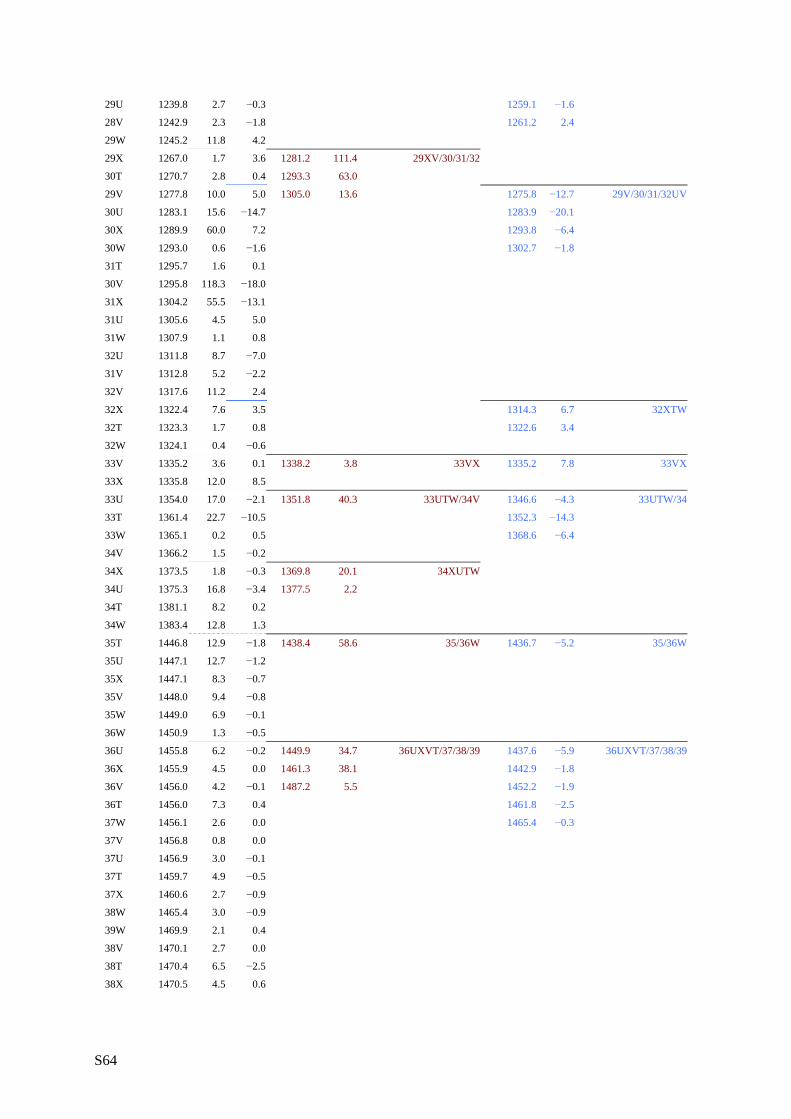
S64
29U 1239.8 2.7 −0.3 1259.1 −1.6
28V 1242.9 2.3 −1.8 1261.2 2.4
29W 1245.2 11.8 4.2
29X 1267.0 1.7 3.6 1281.2 111.4 29XV/30/31/32
30T 1270.7 2.8 0.4 1293.3 63.0
29V 1277.8 10.0 5.0 1305.0 13.6 1275.8 −12.7 29V/30/31/32UV
30U 1283.1 15.6 −14.7 1283.9 −20.1
30X 1289.9 60.0 7.2 1293.8 −6.4
30W 1293.0 0.6 −1.6 1302.7 −1.8
31T 1295.7 1.6 0.1
30V 1295.8 118.3 −18.0
31X 1304.2 55.5 −13.1
31U 1305.6 4.5 5.0
31W 1307.9 1.1 0.8
32U 1311.8 8.7 −7.0
31V 1312.8 5.2 −2.2
32V 1317.6 11.2 2.4
32X 1322.4 7.6 3.5 1314.3 6.7 32XTW
32T 1323.3 1.7 0.8 1322.6 3.4
32W 1324.1 0.4 −0.6
33V 1335.2 3.6 0.1 1338.2 3.8 33VX 1335.2 7.8 33VX
33X 1335.8 12.0 8.5
33U 1354.0 17.0 −2.1 1351.8 40.3 33UTW/34V 1346.6 −4.3 33UTW/34
33T 1361.4 22.7 −10.5 1352.3 −14.3
33W 1365.1 0.2 0.5 1368.6 −6.4
34V 1366.2 1.5 −0.2
34X 1373.5 1.8 −0.3 1369.8 20.1 34XUTW
34U 1375.3 16.8 −3.4 1377.5 2.2
34T 1381.1 8.2 0.2
34W 1383.4 12.8 1.3
35T 1446.8 12.9 −1.8 1438.4 58.6 35/36W 1436.7 −5.2 35/36W
35U 1447.1 12.7 −1.2
35X 1447.1 8.3 −0.7
35V 1448.0 9.4 −0.8
35W 1449.0 6.9 −0.1
36W 1450.9 1.3 −0.5
36U 1455.8 6.2 −0.2 1449.9 34.7 36UXVT/37/38/39 1437.6 −5.9 36UXVT/37/38/39
36X 1455.9 4.5 0.0 1461.3 38.1 1442.9 −1.8
36V 1456.0 4.2 −0.1 1487.2 5.5 1452.2 −1.9
36T 1456.0 7.3 0.4 1461.8 −2.5
37W 1456.1 2.6 0.0 1465.4 −0.3
37V 1456.8 0.8 0.0
37U 1456.9 3.0 −0.1
37T 1459.7 4.9 −0.5
37X 1460.6 2.7 −0.9
38W 1465.4 3.0 −0.9
39W 1469.9 2.1 0.4
38V 1470.1 2.7 0.0
38T 1470.4 6.5 −2.5
38X 1470.5 4.5 0.6

S65
39V 1471.1 4.0 0.6
39T 1471.5 7.5 −0.5
39X 1471.6 4.7 0.0
38U 1471.6 7.4 0.6
39U 1472.2 2.7 −2.8
40U 1495.5 1.5 0.0 1487.2 5.5 40 40
40V 1496.8 0.4 0.0
40W 1499.5 0.0 −0.2
40T 1500.6 0.6 0.5
40X 1502.3 0.4 −0.4
41X 1787.2 89.9 −6.9 1733.9 214.1 41 1729.0 −1.5 41XVW
41V 1791.7 91.0 −5.2 1747.9 405.8
41W 1793.1 40.2 2.0
41T 1804.6 127.8 10.1 1746.0 3.1 41TU
41U 1808.1 114.3 1.4 1750.2 20.1
PBE1PBE1/cc-pVTZ experiment Fund v D R v D Fund v R Fund
21X 1049.0 16.6 2.7 1035.4 9.4 21XVW21V 1062.6 29.5 −1.0 1039.0 65.1 21VW 1045.0 3.8 21W 1064.6 5.5 0.5 1054.4 0.4 22U 1089.0 7.9 3.4 1074.0 81.1 22/23W 1067.8 2.9 22/23W22W 1093.1 18.2 0.3 1075.4 7.7 22T 1094.1 6.5 −4.9 1081.1 7.3 22V 1094.2 37.6 6.8 1085.9 14.0 22X 1097.6 25.4 −10.9 23W 1103.9 35.4 3.5 23X 1128.5 81.2 13.2 1086.6 266.4 23XVTU/24 1098.4 2.2 23XVTU/2423V 1131.8 58.5 2.7 1097.3 193.5 1101.1 2.6 23T 1136.6 165.3 4.5 1108.9 18.0 23U 1141.0 189.3 5.8 24W 1154.1 0.4 0.3 24T 1154.6 0.7 −0.2 24U 1154.7 0.7 −0.5 24X 1154.7 0.6 0.0 24V 1154.9 0.5 0.1 25X 1168.6 29.0 3.2 1176.1 135.5 25/26/27 1163.9 −3.8 25/26/2725W 1171.3 1.0 0.0 1177.2 −19.7 25T 1173.5 111.0 13.5 26X 1177.8 6.2 −1.6 26T 1179.7 3.3 −4.6 26W 1179.9 11.9 −2.2 25U 1181.0 12.8 −5.6 25V 1183.0 5.1 0.1 26V 1185.2 1.3 2.9 26U 1186.4 4.1 −0.9 27T 1188.8 10.3 2.8 27X 1189.7 12.7 0.5 27V 1192.2 7.1 3.7 27W 1192.5 5.8 −1.7 27U 1194.3 21.2 13.0 28T 1217.5 259.9 13.4 1213.6 498.2 28/29TUW 1191.1 2.9 28/29TUWX

S66
28U 1218.5 161.1 22.4 1255.5 77.0 1210.9 31.4 28X 1229.3 11.6 −4.2 1218.5 6.8 28W 1230.7 74.6 1.3 29T 1231.3 14.9 7.9 29U 1235.4 5.5 0.1 28V 1238.7 2.3 −1.4 29W 1241.7 17.3 4.8 29X 1262.0 2.0 4.0 1281.2 111.4 29XV/30/31/32 1238.7 1.3 29X/30T30T 1266.4 3.5 −0.3 1293.3 63.0 1245.6 −1.1
1259.1 −1.6 1261.2 2.4
29V 1272.1 6.8 4.0 1275.8 −12.7 29V/30UXWV/31/32UV30U 1278.0 16.1 −14.7 1283.9 −20.1 30X 1286.4 40.3 7.8 1293.8 −6.4 30W 1287.6 0.8 −1.8 1302.7 −1.8 31T 1289.6 1.9 0.2 30V 1295.6 103.8 −15.9 31U 1299.1 4.7 4.9 31X 1301.0 73.2 −15.3 31W 1303.3 1.2 0.8 32U 1306.6 9.4 −6.9 31V 1307.3 6.2 −2.6 32V 1312.5 21.4 1.9 32X 1317.3 8.9 3.5 1314.3 6.7 32XTW32T 1318.3 2.0 0.9 1322.6 3.4 32W 1319.2 0.3 −0.5 33V 1330.2 4.4 0.0 1338.2 3.8 33VX 1335.2 7.8 33XV33X 1331.5 17.6 9.9 33U 1348.9 16.9 −1.8 1351.8 40.3 33UTW/34 1346.6 −4.3 33UTW/3433T 1356.8 25.5 −11.2 1369.8 20.1 1352.3 −14.3 33W 1359.9 0.2 0.4 1377.5 2.2 1368.6 −6.4 34V 1361.2 1.5 −0.1 34X 1368.8 2.1 −0.1 34U 1371.5 17.0 −3.7 34T 1377.4 10.0 −0.3 34W 1380.2 13.0 1.3 35T 1441.1 15.8 −2.2 1438.4 58.6 35/36/37/38/39 1436.7 −5.2 3535X 1441.4 10.0 −0.8 1449.9 34.7 35U 1441.4 13.7 −1.3 1461.3 38.1 35V 1442.3 10.7 −1.0 35W 1442.7 3.7 −0.5 36W 1444.0 5.7 −0.1 36U 1448.6 5.9 −0.4 1437.6 −5.9 36UXVT/37/38/3936X 1448.8 4.9 0.1 1442.9 −1.8 36V 1448.9 4.2 −0.1 1452.2 −1.9 36T 1448.9 7.9 0.3 1461.8 −2.5 37W 1449.0 2.6 0.1 1465.4 −0.3 37V 1449.1 0.8 0.0 37U 1449.4 3.4 0.1 37T 1452.2 5.9 −0.5 37X 1453.0 3.1 −1.1 38W 1458.1 2.8 −0.9 38V 1462.8 2.8 −0.1 38T 1463.0 7.3 −2.7 39W 1463.3 2.1 0.4

S67
38X 1463.9 5.0 1.2 39X 1464.3 4.8 −0.4 39V 1464.6 3.9 0.7 39T 1464.9 7.9 −0.5 38U 1465.0 7.3 1.8 39U 1465.4 2.5 −3.9 40U 1488.3 1.5 −0.1 1487.2 5.5 40 4040V 1489.4 0.4 0.0 40W 1492.4 0.0 −0.2 40T 1493.3 0.8 0.5 40X 1495.2 0.5 −0.4 41X 1789.0 92.2 −7.2 1733.9 214.1 41 1729.0 −1.5 41XVW41V 1793.5 87.7 −5.1 1747.9 405.8 41W 1794.2 38.2 1.8 41T 1805.3 132.8 11.1 1746.0 3.1 41TU41U 1809.1 106.1 1.7 1750.2 20.1
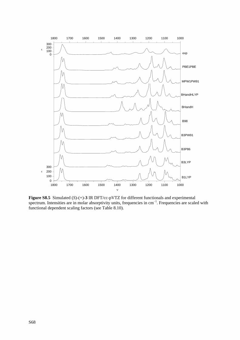
S68
1800 1700 1600 1500 1400 1300 1200 1100 10000
100200300
ν
B3LYP
B3PW91
B3P86
B1LYP
ε
BHandH
BHandHLYP
MPW1PW91
ε
B98
exp
PBE1PBE
0100200300
1800 1700 1600 1500 1400 1300 1200 1100 1000
Figure S8.5 Simulated (S)-(+)-3 IR DFT/cc-pVTZ for different functionals and experimental spectrum. Intensities are in molar absorptivity units, frequencies in cm−1. Frequencies are scaled with functional dependent scaling factors (see Table 8.10).

S69
1800 1700 1600 1500 1400 1300 1200 1100 1000-0.010-0.0050.0000.0050.0100.015
ν
Δ ε
Δ ε
exp
B3LYP
B3PW91
B3P86
B1LYP
BHandH
BHandHLYP
MPW1PW91
B98
PBE1PBE
-0.0050.0000.0050.0100.015
1800 1700 1600 1500 1400 1300 1200 1100 1000
Figure S8.6 Simulated (S)-(+)-3 VCD DFT/cc-pVTZ for different functionals and experimental spectrum. Intensities are in molar absorptivity units, frequencies in cm−1. Frequencies are scaled with functional dependent scaling factors (see Table 8.10).