Copyright (c) 2000 by Harcourt, Inc. All rights reserved. Marginalism Firms as profit maximizers...
53
Copyright (c) 2000 by Harcourt, Inc. All rights reserved. Marginalism • Firms as profit maximizers will make decisions in a marginal way. • The manager looks at the marginal profit from producing one more unit of output or the additional profit from hiring one more unit of labor. • When the incremental profit of an activity becomes zero, profits are maximized.
-
Upload
lydia-fletcher -
Category
Documents
-
view
216 -
download
1
Transcript of Copyright (c) 2000 by Harcourt, Inc. All rights reserved. Marginalism Firms as profit maximizers...

Copyright (c) 2000 by Harcourt, Inc. All rights reserved.
Marginalism
• Firms as profit maximizers will make decisions in a marginal way.
• The manager looks at the marginal profit from producing one more unit of output or the additional profit from hiring one more unit of labor.
• When the incremental profit of an activity becomes zero, profits are maximized.

Copyright (c) 2000 by Harcourt, Inc. All rights reserved.
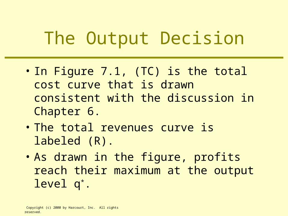
The Output Decision
• Economic profits () are defined as = R(q) - TC(q)
where R(q) is the amount of revenues received and TC(q) are the economic costs incurred, , both depending upon the level of output (q) produced.
• The firm will choose the level of output that generates the largest level of profit.
Copyright (c) 2000 by Harcourt, Inc. All rights reserved.
The Output Decision
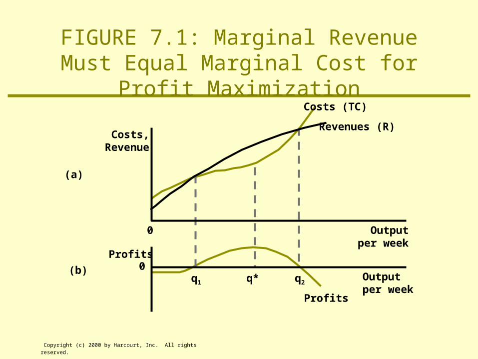
• In Figure 7.1, (TC) is the total cost curve that is drawn consistent with the discussion in Chapter 6.
• The total revenues curve is labeled (R).
• As drawn in the figure, profits reach their maximum at the output level q*.
Copyright (c) 2000 by Harcourt, Inc. All rights reserved.
Costs (TC)
Revenues (R)
Profits
q1 q2q*
Costs,Revenue
(a)
(b)
Profits0
Outputper week
0
FIGURE 7.1: Marginal Revenue Must Equal Marginal Cost for Profit Maximization
Outputper week

Copyright (c) 2000 by Harcourt, Inc. All rights reserved.
The Marginal Revenue/Marginal Cost Rule
• At output levels below q* increasing output causes profits to increase, so profit maximizing firms would not stop short of q*.
• Increasing output beyond q* reduces profits, so profit maximizing firms would not produce more than q*.

Copyright (c) 2000 by Harcourt, Inc. All rights reserved.
The Marginal Revenue/Marginal Cost Rule
• At q* marginal cost equals marginal revenue, the extra revenue a firm receives when it sells one more unit of output.
• In order to maximize profits, a firm should produce that output level for which the marginal revenue from selling one more unit of output is exactly equal to the marginal cost of producing that unit of output.

Copyright (c) 2000 by Harcourt, Inc. All rights reserved.
The Marginal Revenue/Marginal Cost Rule
• At the profit maximizing level of output Marginal Revenue = Marginal
Cost or MR = MC.
• Firms, starting at zero output, can expand output so long as marginal revenue exceeds marginal cost, but don’t go beyond the point where these two are equal.

Copyright (c) 2000 by Harcourt, Inc. All rights reserved.
Marginalism in Input Choices
• Both labor and capital should be hired up to the point where the additional revenue brought in by selling the output produced by the extra labor or capital equals the increase in costs brought on by hiring the additional inputs.

Copyright (c) 2000 by Harcourt, Inc. All rights reserved.
Marginal Revenue
• A price taker is a firm or individual whose decisions regarding buying or selling have no effect on the prevailing market price of a good or service.
• For a price taking firm MR = P.

Copyright (c) 2000 by Harcourt, Inc. All rights reserved.
Marginal Revenue for a Downward-Sloping Demand Curve
• A firm that is not a price taker faces a downward sloping demand curve for its product.
• These firms must reduce their selling price in order to sell more goods or services.
• In this case marginal revenue is less than market price
MR < P.
Copyright (c) 2000 by Harcourt, Inc. All rights reserved.
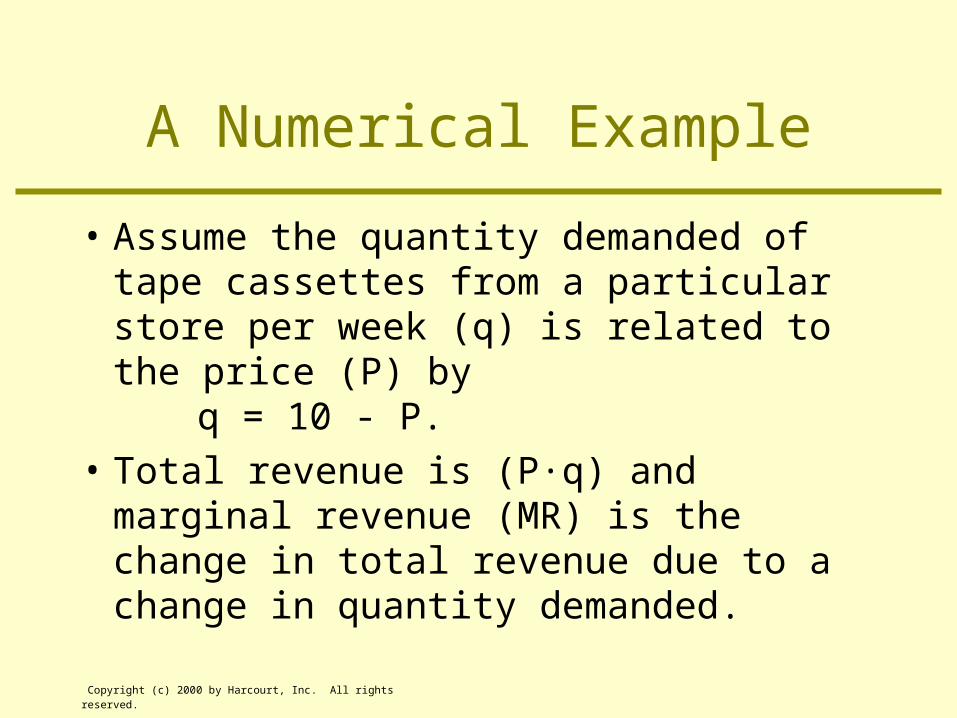
A Numerical Example
• Assume the quantity demanded of tape cassettes from a particular store per week (q) is related to the price (P) by
q = 10 - P.
• Total revenue is (P·q) and marginal revenue (MR) is the change in total revenue due to a change in quantity demanded.

Copyright (c) 2000 by Harcourt, Inc. All rights reserved.
A Numerical Example
• This example demonstrates that MR < P as shown in Table 7.1.
• Total revenue reaches a maximum at q = 5, P = 5.
• For q > 5, total revenues decline causing marginal revenue to be negative.

Copyright (c) 2000 by Harcourt, Inc. All rights reserved.
TABLE 7.1: Total and Marginal Revenue for Cassette Tapes (q = 10 - P)
Price (P) Quantity (q) Total Revenue (P·q) Marginal Revenue (MR)$10 0 $0 9 1 9 $ 9 8 2 16 7 7 3 21 5 6 4 24 3 5 5 25 1 4 6 24 -1 3 7 21 -3 2 8 16 -5 1 9 9 -7 0 10 0 -9

Copyright (c) 2000 by Harcourt, Inc. All rights reserved.
A Numerical Example
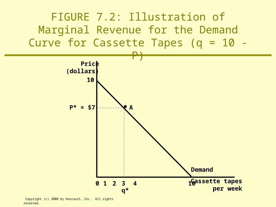
• This hypothetical demand curve is shown in Figure 7.2.
• When q = 3, P = $7 and total revenue equals $21 which is shown by the area of the rectangle P*Aq*0.
• If the firm wants to sell four tapes it must reduce the price to $6.
Copyright (c) 2000 by Harcourt, Inc. All rights reserved.
Price(dollars)
Demand
AP* = $7
10
Cassette tapesper week
1 2 3 4 10q*
0
FIGURE 7.2: Illustration of Marginal Revenue for the Demand Curve for Cassette Tapes (q = 10 - P)
Copyright (c) 2000 by Harcourt, Inc. All rights reserved.
A Numerical Example
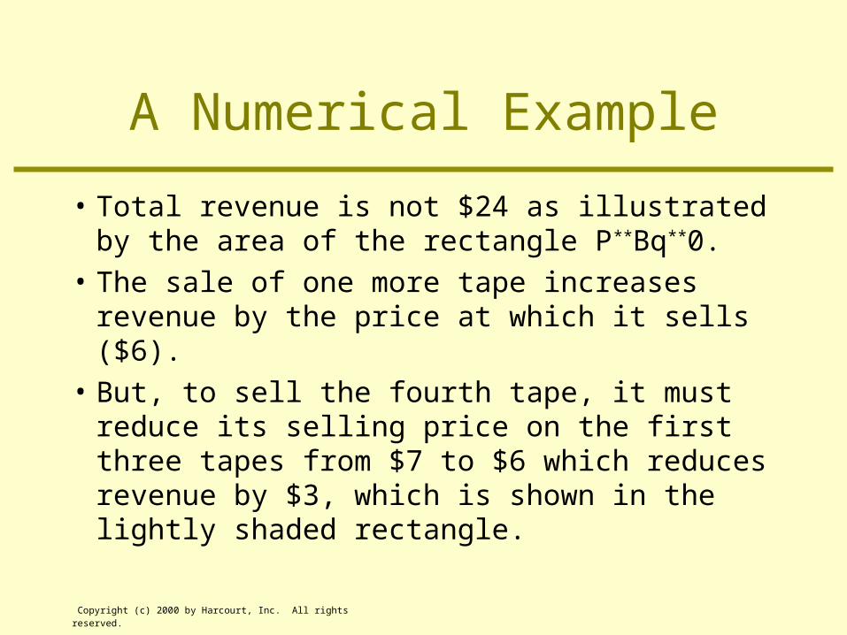
• Total revenue is not $24 as illustrated by the area of the rectangle P**Bq**0.
• The sale of one more tape increases revenue by the price at which it sells ($6).
• But, to sell the fourth tape, it must reduce its selling price on the first three tapes from $7 to $6 which reduces revenue by $3, which is shown in the lightly shaded rectangle.

Copyright (c) 2000 by Harcourt, Inc. All rights reserved.
Price(dollars)
Demand
A
B
P* = $7
10
Cassette tapesper week
1 2 3 4 10q* q**
0
FIGURE 7.2: Illustration of Marginal Revenue for the Demand Curve for Cassette Tapes (q = 10 - P)
P* = $6
Copyright (c) 2000 by Harcourt, Inc. All rights reserved.
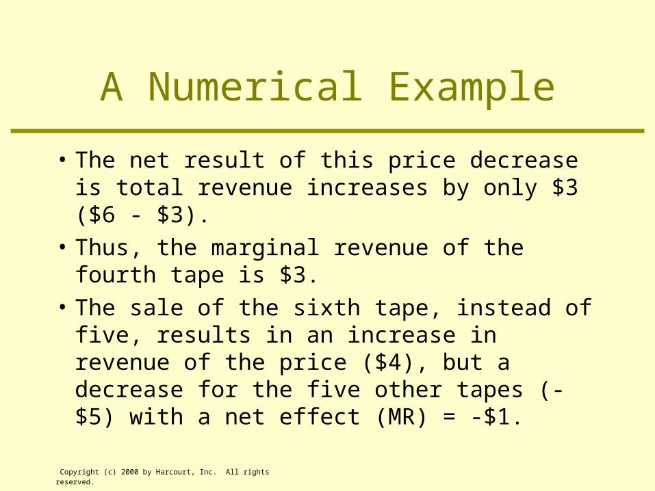
A Numerical Example
• The net result of this price decrease is total revenue increases by only $3 ($6 - $3).
• Thus, the marginal revenue of the fourth tape is $3.
• The sale of the sixth tape, instead of five, results in an increase in revenue of the price ($4), but a decrease for the five other tapes (-$5) with a net effect (MR) = -$1.

Copyright (c) 2000 by Harcourt, Inc. All rights reserved.
TABLE 7.2: Relationship between Marginal Revenue and Elasticity
Demand Curve Marginal Revenue
Elastic (eq,p < -1) MR > 0
Unit elastic (eq,P = -1) MR = 0
Inelastic (eq,P > -1) MR < 0

Copyright (c) 2000 by Harcourt, Inc. All rights reserved.
Marginal Revenue and Price Elasticity
• It can be shown that all of the relationships in Table 7.2 can be derived from the basic equation
PqePMR
,
11
• For example, if eq,P < -1 (elastic), this equation shows that MR is positive.
Copyright (c) 2000 by Harcourt, Inc. All rights reserved.
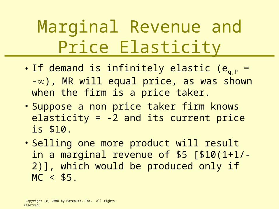
Marginal Revenue and Price Elasticity
• If demand is infinitely elastic (eq,P = -), MR will equal price, as was shown when the firm is a price taker.
• Suppose a non price taker firm knows elasticity = -2 and its current price is $10.
• Selling one more product will result in a marginal revenue of $5 [$10(1+1/-2)], which would be produced only if MC < $5.

Copyright (c) 2000 by Harcourt, Inc. All rights reserved.
Marginal Revenue Curve
• It is sometimes useful to think of the demand curve as the average revenue curve since it shows the revenue per unit (price).
• The marginal revenue curve is a curve showing the relationship between the quantity a firm sells and the revenue yielded by the last unit sold. It is derived from the demand curve.

Copyright (c) 2000 by Harcourt, Inc. All rights reserved.
Marginal Revenue Curve
• With a downward-sloping demand curve, the marginal revenue curve will lie below the demand curve since, at any level of output, marginal revenue is less than price.
• A demand and marginal revenue curve are shown in Figure 7.3.
• For output levels greater than q1, marginal revenue is negative.

Copyright (c) 2000 by Harcourt, Inc. All rights reserved.
Price
Demand (Average Revenue)
Marginal Revenue
P1
Quantityper week
q10
FIGURE 7.3: Marginal Revenue Curve Associated with a Demand Curve

Copyright (c) 2000 by Harcourt, Inc. All rights reserved.
Shifts in Demand and Marginal Revenue Curves
• As previously discussed, changes in such factors as income, other prices, or preferences cause demand curves to shift.
• Since marginal revenue curves are derived from demand curves, whenever the demand curve shifts, the marginal revenue curve also shifts.
Copyright (c) 2000 by Harcourt, Inc. All rights reserved.
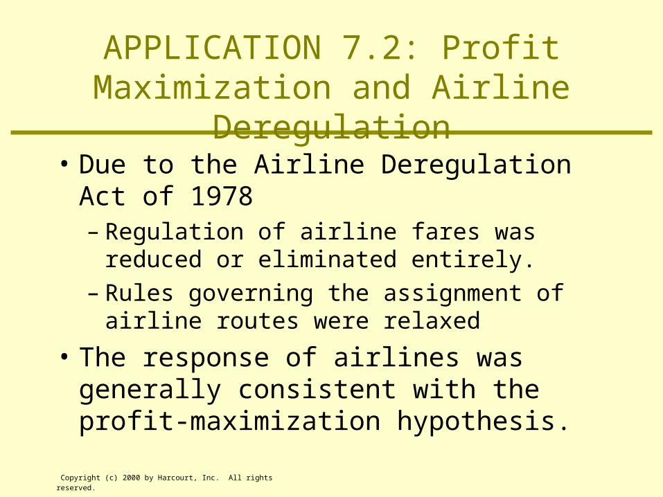
APPLICATION 7.2: Profit Maximization and Airline Deregulation
• Due to the Airline Deregulation Act of 1978– Regulation of airline fares was reduced or
eliminated entirely.– Rules governing the assignment of airline
routes were relaxed
• The response of airlines was generally consistent with the profit-maximization hypothesis.
Copyright (c) 2000 by Harcourt, Inc. All rights reserved.
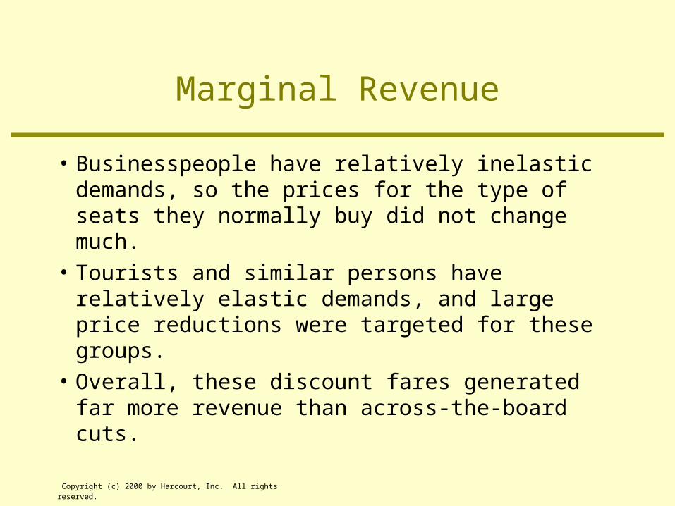
Marginal Revenue
• Businesspeople have relatively inelastic demands, so the prices for the type of seats they normally buy did not change much.
• Tourists and similar persons have relatively elastic demands, and large price reductions were targeted for these groups.
• Overall, these discount fares generated far more revenue than across-the-board cuts.

Copyright (c) 2000 by Harcourt, Inc. All rights reserved.
Marginal Cost
• While fleets of aircraft could not be changed in the short-run, airlines altered their route structure.– Service to many small communities, previously
required by the Civil Aeronautics Board, were curtailed.
– Hub-and-spoke procedures were adopted to allow firms to use different types of aircraft on different routes.
Copyright (c) 2000 by Harcourt, Inc. All rights reserved.
Marginal Cost
• Because the marginal cost associated with filling empty seats on a plane is essentially zero, profits from the last few passengers on a flight are very high.
• Airlines have tried very hard to reduce the losses they suffer from “no shows” by selling more space than is available--overbooking.
Copyright (c) 2000 by Harcourt, Inc. All rights reserved.
Alternatives to Profit Maximization
• Revenue maximization is a goal for firms in which they work to maximize their total revenue rather than profits.
• This goal, proposed by William J. Baumol, is consistent with observed behavior such as higher salaries paid to managers of the largest corporations rather than to managers of the most profitable ones.

Copyright (c) 2000 by Harcourt, Inc. All rights reserved.
APPLCIATION 7.3: Textbook Royalties
• Most authors receive royalties based on total book sales.
• Since royalties are a fixed fraction of total revenues, authors would like their publishers to price their books in such a way as to maximize this total revenue, where marginal revenue equals zero.
Copyright (c) 2000 by Harcourt, Inc. All rights reserved.
Potential Conflicts with Profits
• Because publishers must consider costs, they may wish to publish were marginal cost equals marginal revenue, resulting in a higher price than desired by the author.
• Authors prefer additional resources be invested so long as they increase sales, but publishers want to limit such expenditures due to marginal cost considerations.
Copyright (c) 2000 by Harcourt, Inc. All rights reserved.
Markup Pricing
• Markup pricing is determining the selling price of a good by adding a percentage to the average cost of producing it.
• For example, a 50 percent markup would set the price of the good at 1.5 times average total cost.
• How does this relate to profit maximization?

Copyright (c) 2000 by Harcourt, Inc. All rights reserved.
Price
P* = MR
P**
AP***P1
0Quantityper week
SAC
SMC
E
F
q1 q*** q* q**
FIGURE 7.5: Short-Run Supply Curve for a Price-Taking Firm

Copyright (c) 2000 by Harcourt, Inc. All rights reserved.
The Firm’s Supply Curve
• The firm’s short-run supply curve is the relationship between price and quantity supplied by a firm in the short-run.
• For a price-taking firm, this is the positively sloped portion of the short-run marginal cost curve.
• For all possible prices, the marginal cost curve shows how much output the firm should supply.

Copyright (c) 2000 by Harcourt, Inc. All rights reserved.
The Shutdown Decision
• For very low prices, the firm could also produce zero output.
• Since fixed costs are incurred whether or not the firm produces any goods, the decision to produce is based on short-run variable costs.
Copyright (c) 2000 by Harcourt, Inc. All rights reserved.
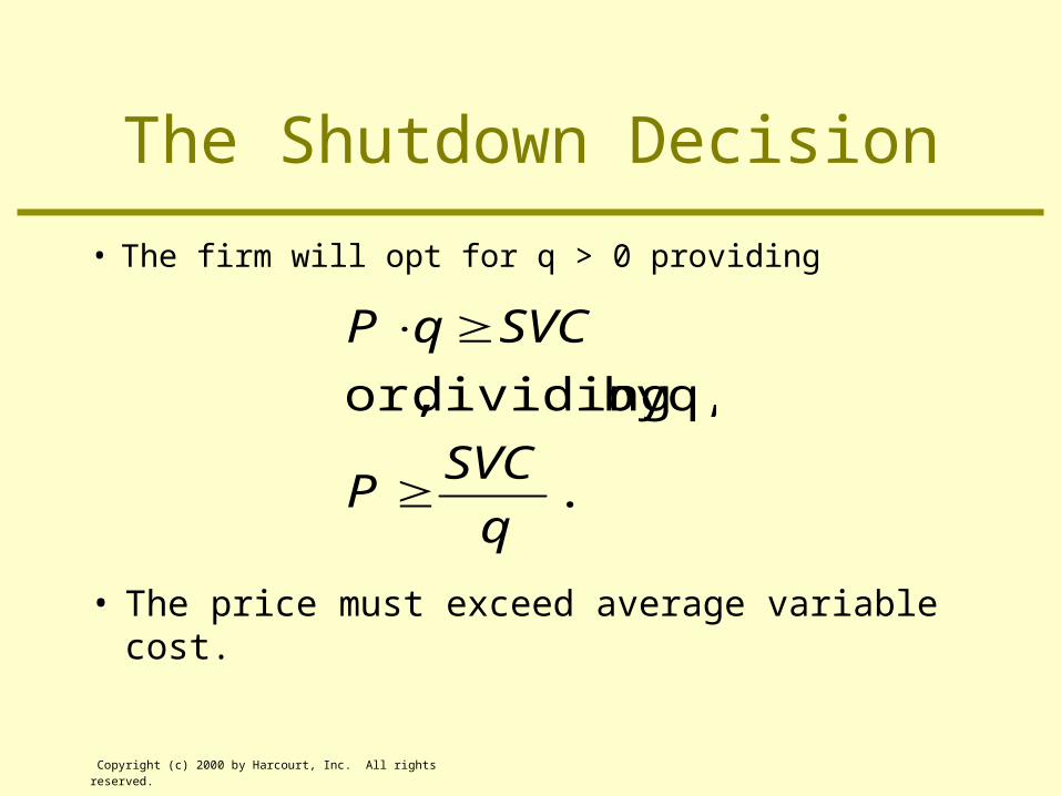
The Shutdown Decision
• The firm will opt for q > 0 providing
• The price must exceed average variable cost.
.
q,by dividing or,
q
SVCP
SVCqP
Copyright (c) 2000 by Harcourt, Inc. All rights reserved.
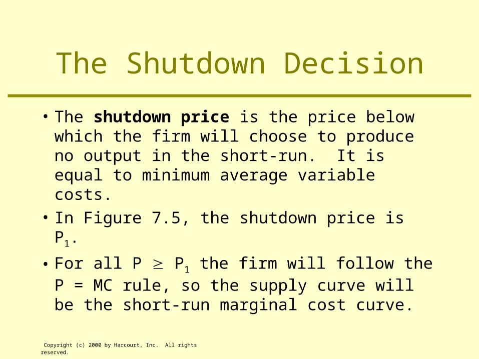
The Shutdown Decision
• The shutdown price is the price below which the firm will choose to produce no output in the short-run. It is equal to minimum average variable costs.
• In Figure 7.5, the shutdown price is P1.
• For all P P1 the firm will follow the P = MC rule, so the supply curve will be the short-run marginal cost curve.

Copyright (c) 2000 by Harcourt, Inc. All rights reserved.
Profit Maximization and Managers’ Incentives
• The principal-agent relationship is an economic actor (the principal) delegating decision-making authority to another party (the agent).
• As early as Adam Smith, it was understood that managers of a company may have different goals than are the goals of the owners of the company.

Copyright (c) 2000 by Harcourt, Inc. All rights reserved.
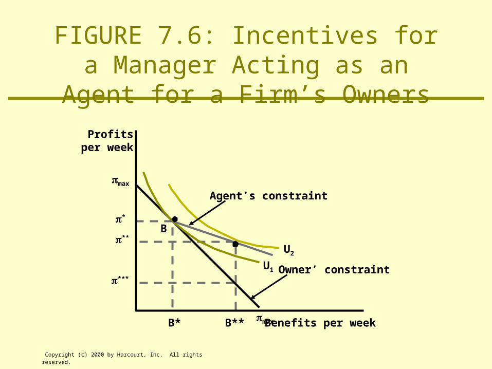
A Model of the Principal-Agent Relationship
• Figure 7.6 shows the indifference curve map of a manager’s preferences between the firm’s profits (the primary interest of the owners) and various benefits that accrue mainly to the manager.
• Assuming the manager is also the owner, if the manager chooses no special benefits, profits will be max.

Copyright (c) 2000 by Harcourt, Inc. All rights reserved.
A Model of the Principal-Agent Relationship
• Each dollar of benefits received by the manger reduces profits by one dollar.
• The slope of the budget constraint is -1, and profits will be zero when benefits equal max.
• The owner-manager maximizes utility at *, B* which, which is somewhat less than max.

Copyright (c) 2000 by Harcourt, Inc. All rights reserved.
Profitsper week
B
max
Benefits per week
Owner’ constraintU1
B*
FIGURE 7.6: Incentives for a Manager Acting as an Agent for a Firm’s Owners
max
*
Copyright (c) 2000 by Harcourt, Inc. All rights reserved.
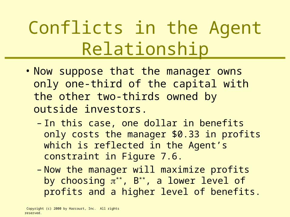
Conflicts in the Agent Relationship
• Now suppose that the manager owns only one-third of the capital with the other two-thirds owned by outside investors.– In this case, one dollar in benefits only costs the
manager $0.33 in profits which is reflected in the Agent’s constraint in Figure 7.6.
– Now the manager will maximize profits by choosing **, B**, a lower level of profits and a higher level of benefits.
Copyright (c) 2000 by Harcourt, Inc. All rights reserved.
Profitsper week
B
max
Benefits per week
Owner’ constraint
Agent’s constraint
U1
U2
B* B**
FIGURE 7.6: Incentives for a Manager Acting as an Agent for a Firm’s Owners
max
*
***
**
Copyright (c) 2000 by Harcourt, Inc. All rights reserved.
Conflicts in the Agent Relationship
• However, **, B** is not attainable by the firm, so profits will actually be ***.
• The other owners have been harmed by relying on an agency relationship.– It appears that the smaller the ownership by the
manager, the greater the reduction in profits.
• Other agent conflicts studied by economists include investment managers and automobile mechanics.
Copyright (c) 2000 by Harcourt, Inc. All rights reserved.
APPLICATION 7.5: Principals and Agents in Franchising
• Many large business, such as McDonald’s Corporation, operate their local retail outlets through franchise contracts.– For example, local McDonalds restaurants are
usually owned by local groups of investors.
• The problem for the parent company is to ensure that their franchise agents operate in a proper manner.
Copyright (c) 2000 by Harcourt, Inc. All rights reserved.
APPLICATION 7.5: Principals and Agents in Franchising
• Various provisions of franchise contracts help to assure proper behavior.– With McDonald’s franchises, for example,
must meet food-quality and service standards and must purchase supplies from firms that meet standards set by the parent company.
– The franchisee, in return, gets some management assistance and national advertising and gets to keep a large share of the profits.

Copyright (c) 2000 by Harcourt, Inc. All rights reserved.
APPLICATION 7.5: Principals and Agents in Medicine
• Physicians act as agents for patients who often lack knowledge of their illness or what treatments are warranted.
• There are several reasons why physicians might not chose exactly what a fully informed patient might choose.– Unlike the physician, the patient must pay the
medical bills.

Copyright (c) 2000 by Harcourt, Inc. All rights reserved.
APPLICATION 7.5: Principals and Agents in Medicine
– Since the physician is usually the care provider, he or she may financially benefit from the services provided.
– Studies find evidence of this physician induced demand, especially for patients with insurance.
• Doctors are “double agents” with insured patients since they represent both the patients and the insurance company.

Copyright (c) 2000 by Harcourt, Inc. All rights reserved.
APPLICATION 7.5: Principals and Agents in Medicine
• Current controversies, such as the growth of managed care organizations arise from this dual relationship.– The rapid escalation of health costs have
resulted in managed care organizations.– Alternatively, restrictions place by managed
care organizations have resulted in a major backlash among patients.

Copyright (c) 2000 by Harcourt, Inc. All rights reserved.
APPLICATION 7.6: Stock Options
• Stock options grant the holder the ability to buy shares at a fixed price.
• If the market price of the shares increases, the holder will benefit by buying at the option price and selling at the higher price.
• Firms grand options to their executives as incentives to manage the firm in a way that leads to increases in stock value.

Copyright (c) 2000 by Harcourt, Inc. All rights reserved.
APPLICATION 7.6: The Explosion of Stock Options
• While stock options were uncommon in the 1980s, by the 1990s top executives of the largest companies received more than half their total compensation in the form of stock options.
• Reasons for this increase in the use of options include– Rising stock prices made this option attractive.

Copyright (c) 2000 by Harcourt, Inc. All rights reserved.
APPLICATION 7.6: The Explosion of Stock Options
– Since options are often assigned a zero cost to the firm, they made a low-cost way to pay their executives.
– A special provision of the tax laws enacted in 1993 limited deductions of executive pay to no more than $1 million per year, unless pay was tied to company performance--which increased the incentive to use stock options.