Copyright

by

Venktesh Pandey

2016

The Thesis Committee for Venktesh Pandey

Certifies that this is the approved version of the following thesis:

Optimal Dynamic Pricing for Managed Lanes with

Multiple Entrances and Exits

APPROVED BY

SUPERVISING COMMITTEE:

Supervisor:Stephen D. Boyles

Christian Claudel

Optimal Dynamic Pricing for Managed Lanes with

Multiple Entrances and Exits

by

Venktesh Pandey, B.Tech

Thesis

Presented to the Faculty of the Graduate School of

The University of Texas at Austin

in Partial Fulfillment

of the Requirements

for the Degree of

Master of Science in Engineering

The University of Texas at Austin

August 2016

To ‘The School of Life’

Acknowledgements

This thesis is a product of many forces and inspirations: some of which im-

pacted me very directly, while the other influenced me in many unknown but deeply

profound ways. An attempt is made to offer an acknowledgment to some of those.

I convey my special thanks to my adviser Dr. Stephen Boyles for his amazing

guidance and advice all throughout the past two years. His suggestions and insights

made it possible for me to realize the broad goals of research and helped me stay

motivated when things did not appear very optimistic. I will always be thankful to

his ways of explaining the difficult concepts, either as part of a classroom teaching or

during the several of our research group meetings, that made the learning seem very

natural and made my interest in the field of transportation more deep.

I am thankful to all the other faculty in the Transportation Engineering Pro-

gram, who helped me broaden my understanding of the field in form of courses and

lectures. Special thanks to Dr. Humphreys and Dr. Bakolas in the Aerospace Engi-

neering Program who with their insightful teaching in the field of optimal control and

stochastic estimation, built my interest into choosing this topic as my thesis. I am

also thankful to Dr. Gopal R Patil for introducing me to the field of transportation

research in my undergraduate.

I convey my acknowledgment and thanks to all my current and past research

group members: Tarun, Ehsan, Michael, Sudesh, Rachel, John, Tyler, Rebecca,

Rahul, and Tejas. They all motivated and inspired me in a number of ways. Special

thanks to Tarun for giving shape to many of my preliminary vague ideas, some of

which took the form of thesis as it stands now.

This list of acknowledgment would be far away from completion if I did not

mention the support of all my friends in US who helped me stay sane, healthy, and

v

mentally strong in many a difficult times: Rachel, John, Kristie, Alice, Vivek, Vatsal,

Nitin, Devesh, Felipe, Priyadarshan and Jeremy. Special thanks to Rachel for being

a very dear friend who made the journey through the graduate school much more

hopeful, optimistic and fun. I also convey my thanks to everyone in my marathon

training group and the members of the Association for India’s Development who

helped me feel motivated and stay connected to the issues that often become obscure

in the maddening rush of the modern life.

A special thanks to my friends and family in India, who continued to cheer

me up while being thousands of miles away. A heartfelt thanks to my sisters without

whose support and motivation, I would not have sailed through many a difficult

challenges. Last but not the least, I am deeply grateful to my parents for being the

source of love and motivation in my life.

vi

Abstract

Optimal Dynamic Pricing for Managed Lanes with Multiple

Entrances and Exits

Venktesh Pandey, MSE

The University of Texas at Austin, 2016

Supervisor: Stephen D. Boyles

Dynamic pricing models are explored in this thesis for high-occupancy/toll

(HOT) lanes, which are increasingly being considered as a means to relieve congestion

by providing a reliable travel time alternative to travelers. The work is focused on

two aspects of dynamic pricing: (a) utilizing real-time traffic measurements to inform

parameters of the pricing model and (b) developing a optimal pricing formulation for

managed lanes with multiple entrances and exits.

The first part of the thesis develops a non-linear estimation model to determine

the parameters of the value of time (VOT) distribution using real-time loop detector

measurements. The estimation model is run on a HOT network with a single entrance

and exit assuming the VOT has a Burr distribution. The estimation results show that

the true parameter values of a VOT distribution for a population can be learned from

loop detector readings measured before and after the toll gantry location. Differing

toll profile predictions are observed for different choices of initial conditions. The

observability of the collected measurements to estimate the parameters of the model

is identified as a primary factor for the non-linear estimation to work in real-time.

Further research areas are identified to extend the analysis of using real-time loop

detector data for complex HOT networks and for different toll optimization objectives.

vii

The second part proposes a dynamic programming (DP) formulation to solve

distance-based optimal tolling for HOT lanes with multiple entrances and exits (HOT-

MEME) under deterministic demand conditions. The simplifying assumptions made

to model HOT-MEME networks found in the literature are relaxed. Two objectives

are considered for optimization: maximizing generated revenue and minimizing expe-

rienced total system travel time. A spatial queue model is used to capture the traffic

dynamics and a multinomial logit model is used to simulate lane choice at each di-

verge. A backward recursion algorithm is applied, under simplifying assumptions for

the definition of the state of the system, to solve for the optimal toll. The results in-

dicate that the DP approach can theoretically determine optimal tolls for HOT lanes

with multiple entrances and exits, but further research needs to be conducted for the

algorithm to work practically for medium to large size networks. Recommendations

are made in the conclusion about how advanced methods can be utilized to tackle

the computational constraints.

Keywords: Managed lanes, Dynamic pricing, HOT lane with multiple en-

trances and exits, Non-linear estimation, Loop detector data

viii

Table of Contents

List of Tables xii

List of Figures xiii

1 Introduction 1

1.1 Background . . . . . . . . . . . . . . . . . . . . . . . . . . . . . . . . 1

1.2 Motivation . . . . . . . . . . . . . . . . . . . . . . . . . . . . . . . . . 3

1.3 Objectives . . . . . . . . . . . . . . . . . . . . . . . . . . . . . . . . . 4

1.4 Organization of Thesis . . . . . . . . . . . . . . . . . . . . . . . . . . 5

2 Literature Review 7

2.1 Pricing Techniques for Managed Lanes . . . . . . . . . . . . . . . . . 7

2.2 Modeling Managed Lanes . . . . . . . . . . . . . . . . . . . . . . . . 8

2.2.1 Lane Choice Model . . . . . . . . . . . . . . . . . . . . . . . . 9

2.2.2 Traffic Flow Model . . . . . . . . . . . . . . . . . . . . . . . . 13

2.2.3 Toll Pricing Model . . . . . . . . . . . . . . . . . . . . . . . . 14

2.2.4 Demand Model . . . . . . . . . . . . . . . . . . . . . . . . . . 16

2.2.5 Summary Table . . . . . . . . . . . . . . . . . . . . . . . . . . 16

2.3 Data Requirements . . . . . . . . . . . . . . . . . . . . . . . . . . . . 18

2.4 Modeling Managed Lanes Corridor with Multiple Entrances and Exits 19

2.5 Summary . . . . . . . . . . . . . . . . . . . . . . . . . . . . . . . . . 21

3 Estimation for Single Entrance Single Exit Managed Lane 23

3.1 Background . . . . . . . . . . . . . . . . . . . . . . . . . . . . . . . . 23

3.2 Estimation and Toll Optimization in Real Time . . . . . . . . . . . . 25

3.2.1 Notations . . . . . . . . . . . . . . . . . . . . . . . . . . . . . 25

3.2.2 Assumptions . . . . . . . . . . . . . . . . . . . . . . . . . . . . 26

ix

3.2.3 Estimation Model . . . . . . . . . . . . . . . . . . . . . . . . . 27

3.2.4 Toll Update Model . . . . . . . . . . . . . . . . . . . . . . . . 30

3.2.5 Combined Estimation and Optimization . . . . . . . . . . . . 31

3.3 Simulation and Results . . . . . . . . . . . . . . . . . . . . . . . . . . 32

3.4 Summary . . . . . . . . . . . . . . . . . . . . . . . . . . . . . . . . . 36

4 Problem Formulation for Multiple Entrance Multiple Exit HOT

Lanes 38

4.1 Characteristics of HOT lanes with Multiple Entrances and Exits . . . 38

4.1.1 Information at Each Decision Point . . . . . . . . . . . . . . . 39

4.1.2 En-route vs Fixed Decision Making . . . . . . . . . . . . . . . 40

4.1.3 Toll Policy . . . . . . . . . . . . . . . . . . . . . . . . . . . . . 40

4.1.4 Reporting Instantaneous vs Experienced Travel Times . . . . 41

4.2 Optimization Problem . . . . . . . . . . . . . . . . . . . . . . . . . . 41

4.2.1 Notations . . . . . . . . . . . . . . . . . . . . . . . . . . . . . 42

4.2.2 Lane Choice Model . . . . . . . . . . . . . . . . . . . . . . . . 43

4.2.3 Traffic Flow Model . . . . . . . . . . . . . . . . . . . . . . . . 44

4.2.4 Toll Pricing Optimization Model . . . . . . . . . . . . . . . . 49

4.3 Dynamic Programming Formulation . . . . . . . . . . . . . . . . . . . 52

4.3.1 Assumptions . . . . . . . . . . . . . . . . . . . . . . . . . . . . 52

4.3.2 State Space, Action Space, and Value Function . . . . . . . . 53

4.3.3 Backward Recursion Algorithm . . . . . . . . . . . . . . . . . 55

4.4 Summary . . . . . . . . . . . . . . . . . . . . . . . . . . . . . . . . . 58

5 Results 61

5.1 Application of the Dynamic Programming Algorithm . . . . . . . . . 61

5.2 Additional experiments . . . . . . . . . . . . . . . . . . . . . . . . . . 66

5.2.1 Comparing the Performance of the Logit Choice Model and

VOT Distribution . . . . . . . . . . . . . . . . . . . . . . . . . 66

x

5.2.2 Evaluating Performance over Different Network Sizes . . . . . 68

5.2.3 Myopic Revenue Tolling Performance . . . . . . . . . . . . . . 70

5.3 Summary . . . . . . . . . . . . . . . . . . . . . . . . . . . . . . . . . 73

6 Conclusions and Future Scope 75

6.1 Conclusions . . . . . . . . . . . . . . . . . . . . . . . . . . . . . . . . 75

6.2 Future Work . . . . . . . . . . . . . . . . . . . . . . . . . . . . . . . . 76

Bibliography 78

xi

List of Tables

2.1 Choice of particular models for modeling managed lanes in the literature 17

3.1 List of symbols used in estimation model . . . . . . . . . . . . . . . . 26

3.2 Demand values for the simulation . . . . . . . . . . . . . . . . . . . . 33

4.1 List of symbols for the optimization problem . . . . . . . . . . . . . . 43

4.2 List of symbols for the backward recursion algorithm . . . . . . . . . 56

5.1 Performance of DP over different network sizes . . . . . . . . . . . . . 69

xii

List of Figures

1.1 Current pricing schemes on managed lane projects in United States

(Source- NCHRP [1]) . . . . . . . . . . . . . . . . . . . . . . . . . . . 3

1.2 Commonly used heuristics for dynamic tolling of managed lanes (Source-

Michalaka et al. [2]) . . . . . . . . . . . . . . . . . . . . . . . . . . . 4

3.1 Loop detector locations (Source- Lou et al. [3]) . . . . . . . . . . . . 26

3.2 Toll variations obtained for different cases . . . . . . . . . . . . . . . 34

3.3 Estimated parameter values for different cases . . . . . . . . . . . . . 34

3.4 Average corridor travel time for different cases, and the case when true

values are known at the start of the simulation . . . . . . . . . . . . . 35

4.1 Managed lanes corridor with multiple entrances and exits . . . . . . . 39

4.2 Spatial queue model fundamental diagram . . . . . . . . . . . . . . . 45

4.3 Possible types of nodes in a HOT system: (a) merge node, (b) diverge

node, (c) series node, (d) origin node, and (e) destination node . . . . 46

4.4 Pictorial representation of the backward recursion algorithm . . . . . 57

5.1 Single entrance single exit network used in simulation and the associ-

ated fundamental diagram . . . . . . . . . . . . . . . . . . . . . . . . 62

5.2 Plot of the revenue and the TSTT obtained from the DP algorithm

compared against all the enumerated toll profiles . . . . . . . . . . . . 63

5.3 Optimal toll for simulation 1 . . . . . . . . . . . . . . . . . . . . . . . 64

5.4 Optimal toll for simulation 2 . . . . . . . . . . . . . . . . . . . . . . . 65

5.5 N value plot for the HOT and the GP lanes for simulation 2 revenue

maximization objective . . . . . . . . . . . . . . . . . . . . . . . . . . 65

5.6 (a) Revenue collected from different choice models; (b) Proportion us-

ing the HOT lane predicted by each choice model at the optimal tolling 67

xiii

5.7 Four networks considered for testing the impact of network size on the

computational performance of the DP algorithm . . . . . . . . . . . . 69

5.8 Comparison of the myopic tolling policy with the optimal toll . . . . 72

5.9 Performance of myopic tolling for high and low values of demand . . . 73

xiv

Chapter 1

Introduction

1.1 Background

Managing traffic congestion is a growing challenge for transportation planners.

The United States lost around $121 billion in net worth in the year 2011 directly

attributable to congestion on roadway facilities [4]. Congestion is especially a problem

while traveling under time constraints. One can often find people complaining about

getting stuck in traffic while waiting to reach an airport or arrive at a meeting on

time. Reliable travel is the growing need of the hour [5].

One way to improve travel time reliability is by constructing managed lanes.

A managed lane project sets apart a set of lanes “where operational strategies are

proactively implemented and managed in response to changing conditions” to provide

reliable travel time to the road user [6]. A subcategory of managed lanes are priced

managed lanes, which are also referred as express lanes or high-occupancy/toll (HOT)

lanes, where the user has to pay a toll for utilizing the facility.

There has been a great emphasis on priced managed lanes in recent years on

US roadways because of their ability to provide reliable travel time while exploiting

the users’ willingness to pay to generate revenue for infrastructure projects. They also

promote the usage of the transit by providing faster travel time for transit vehicles.

Priced managed lanes are either under consideration or in operation in many major

cities; there were 24 operational managed lane projects in US in 2014, with another

23 in planning or under construction [7]. Reliability of the travel time has been one

of the biggest contributing factors in the success of managed lanes; the utility that

1

an extra lane can offer during emergencies is immense.

As managed lanes solve congestion problems and gain popularity, networks of

managed lanes have become increasingly complex. Managed lanes now have multiple

entrances and exits, and can span an entire corridor length across a city. The LBJ

TEXpress Lanes, which constitute a corridor of managed lanes in Dallas, Texas, fea-

ture 15 entrance ramps and 16 exit ramps along the 13.3-mile stretch of the roadway

[8]. Networks of managed lanes can coexist together with one corridor merging into

another. Given the widespread adoption of electronic tolling and dynamic tolling

based on real-time measurements, toll on managed lanes can now adapt to current

traffic conditions.

These complications are difficult to accommodate in practice. Managed lane

operations have now become more complicated than in the past as they are now

multiobjective and seek to enhance the HOT lane efficiency and utilization, provide

travel time reliability, and yield sufficient revenue to offset the lifecycle costs of the

project [1]. Determining the toll rates dynamically to achieve these objectives remains

one of the primary questions for complex managed lane networks.

The current pricing schemes for tolling HOT lanes used in practice can be

broadly categorized into two categories: schemes following a pre-determined toll

schedule and schemes following a dynamic rate of change of tolls based on real-time

measurements.

Dynamic tolling, which updates the toll based on the real-time congestion

pattern, provides several benefits. Its ability to capture congestion dynamically makes

it a preferred choice in providing reliable travel time across a corridor. It also includes

the capability of setting tolls to achieve a particular objective; thus, the system

can be driven towards optimality. Even though dynamic pricing requires complex

detection and signing, it is increasingly being considered by HOT projects constructed

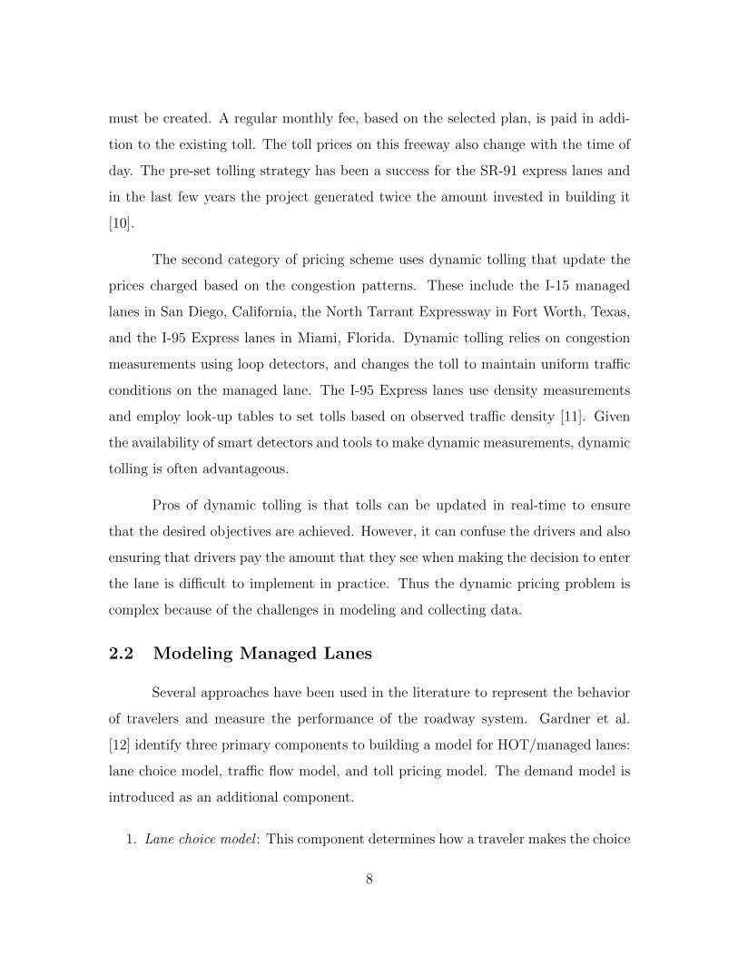
as public private partnerships. Figure 1.1 shows the various types of tolling schemes

2

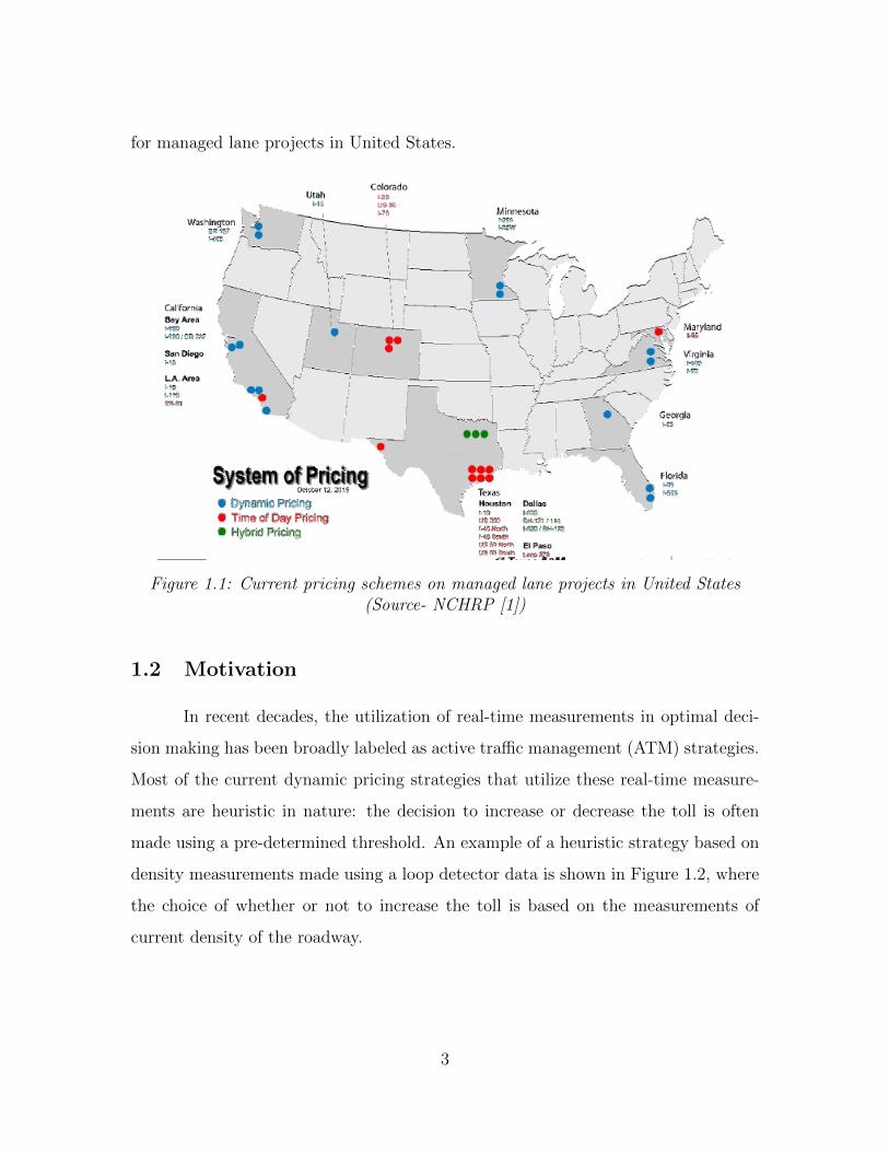
for managed lane projects in United States.

Figure 1.1: Current pricing schemes on managed lane projects in United States(Source- NCHRP [1])

1.2 Motivation

In recent decades, the utilization of real-time measurements in optimal deci-

sion making has been broadly labeled as active traffic management (ATM) strategies.

Most of the current dynamic pricing strategies that utilize these real-time measure-

ments are heuristic in nature: the decision to increase or decrease the toll is often

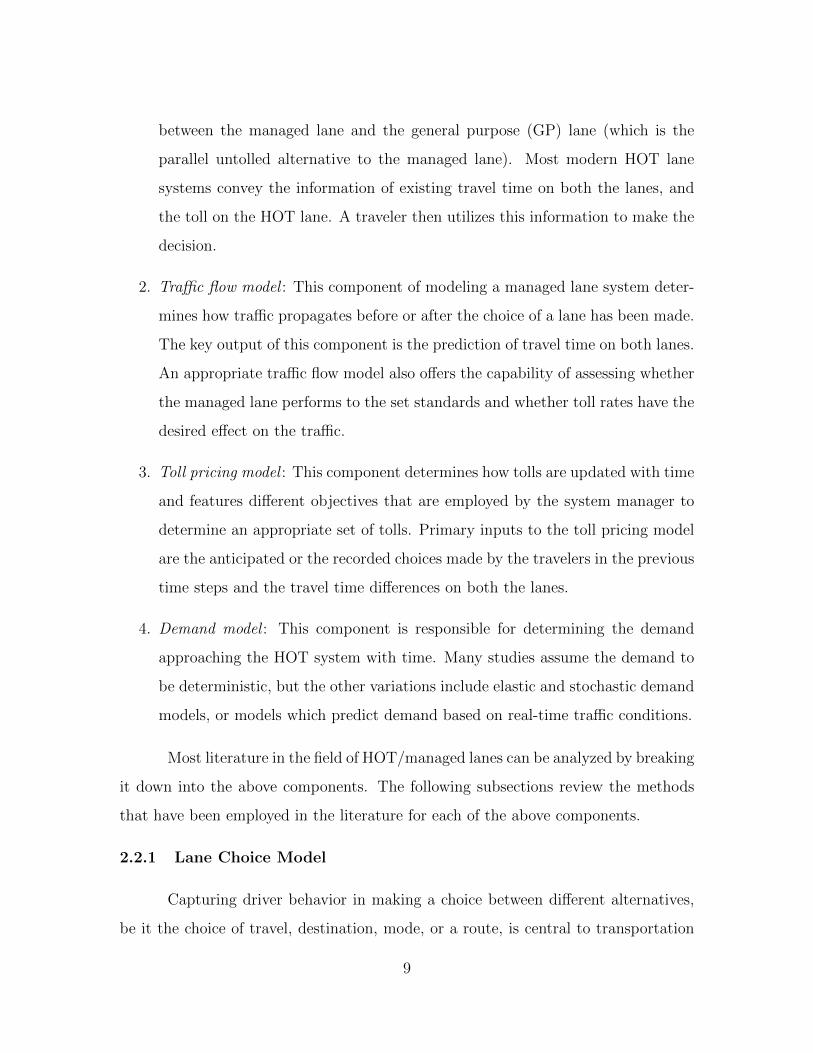
made using a pre-determined threshold. An example of a heuristic strategy based on

density measurements made using a loop detector data is shown in Figure 1.2, where

the choice of whether or not to increase the toll is based on the measurements of

current density of the roadway.

3

Figure 1.2: Commonly used heuristics for dynamic tolling of managed lanes(Source- Michalaka et al. [2])

These heuristics can be potentially improved and tolls can be dynamically

updated to achieve a particular objective. Researchers have primarily focused on

HOT lanes with a single entrance and a single exit (HOT-SESE). Such systems are

easier to model because there is only one decision point for the traveler and the tolls

influence this decision only once. However, for HOT lanes with multiple entrances

and multiple exits (HOT-MEME), there are multiple decision points located at each

diverge location. In such cases, it is complicated to model the behavior of a traveler

and update the tolls that still achieve a particular system-wide objective.

The primary motivation behind the work in this thesis is to develop meth-

ods to determine optimal dynamic tolls for HOT lanes with multiple entrances and

exits. It also seeks to determine optimal tolling decisions using real-time loop de-

tector measurements without making prior assumptions about the demand or other

characteristics of a HOT system.

1.3 Objectives

The dynamic pricing analysis is performed on managed lane networks with

increasing level of complexity. The first part of this thesis focuses on developing

4

a non-linear estimation model for a HOT lane with a single entrance and exit. In

this model, the parameters of the assumed value of time distribution of the travelers

are estimated to determine optimal value of tolls using the real-time loop detector

measurements. The second part focuses on formulating the optimization problem for

a HOT lane network with multiple entrances and exits and developing a dynamic

programming formulation that predicts the optimal tolls for such networks.

Here are the specific objectives considered under this thesis, answers to which

constitute the primary contribution of this research:

1. Estimation problem for a HOT-SESE network : This steps involves formulat-

ing and solving the estimation problem for determining the VOT distribution

parameters for a HOT-SESE network using real-time loop detector data.

2. Defining the optimization problem for finding the optimal toll of a HOT-MEME

network : This step involves selecting a lane choice model and a traffic flow model

to define an optimization problem for finding optimal tolls under the selected

assumptions of driver behavior and traffic flow. Two objectives are considered:

revenue maximization and total system travel time (TSTT) minimization.

3. Developing a dynamic programming formulation for the proposed optimization

problem: This step defines state space, action space, and value functions as

part of the DP formulation. It then uses the backward recursion algorithm to

determine optimal tolls such that the transition through the states achieves the

particular objective. Simulation tests are conducted to assess the performance

of the proposed formulation and validate its optimality.

1.4 Organization of Thesis

The rest of the thesis is organized as follows. Chapter 2 provides a literature

review of the problem of determining optimal tolls for HOT-SESE and HOT-MEME

networks and on the usage of real-time loop detector data to calibrate HOT pricing

5

models. Chapter 3 formulates the problem of performing estimation using real-time

measurements on a HOT-SESE network and presents the results from the analy-

sis. Chapter 4 provides the background for the optimization problem for multiple

entrances and exits and develops the dynamic programming formulation for the max-

imum revenue and minimum TSTT objective. Chapter 5 presents the results of the

analysis performed on different test networks and identifies the advantages and short-

comings of the proposed approach. Chapter 6 summarizes the findings and discusses

the scope for future work.

6

Chapter 2

Literature Review

The idea of internalizing the externality that a traveler imposes on a trans-

portation system by charging appropriate tolls was first introduced by Pigou [9].

Managed lanes are different from regular link tolls as they are imposed with the ob-

jective of providing reliable travel time to the travelers while still ensuring the toll

free option. Several methods in literature have focused on modeling a system with

a HOT lane. The goal of this chapter is to provide a background of the prior work

done in the field of priced managed lanes.

2.1 Pricing Techniques for Managed Lanes

Managed lanes have been implemented in various formats across the world.

Primarily in the US, where 24 priced managed lane projects are functional, different

practices have been used for charging tolls. Tolling schemes can be broadly classified

into two categories: fixed tolling and dynamic tolling based on real-time measure-

ments.

The first category involves collecting pre-determined tolls for using the man-

aged lanes, which are either held constant throughout or are varied by time of day.

Examples include I-10 in Katy, Texas, I-35W in Minneapolis, Minnesota, and I-25

in Denver, Colorado. The I-10 managed lanes in Katy, Texas, admit high-occupancy

vehicles for free during special hours, while levy a toll which varies with time of day

for other vehicles. This time-varying toll reflects the changes in travel volume. The

SR-91 Orange County managed lanes project in California employs an interactive

pricing strategy. To use their facility, a transponder must be installed and an account

7

must be created. A regular monthly fee, based on the selected plan, is paid in addi-

tion to the existing toll. The toll prices on this freeway also change with the time of

day. The pre-set tolling strategy has been a success for the SR-91 express lanes and

in the last few years the project generated twice the amount invested in building it

[10].

The second category of pricing scheme uses dynamic tolling that update the

prices charged based on the congestion patterns. These include the I-15 managed

lanes in San Diego, California, the North Tarrant Expressway in Fort Worth, Texas,

and the I-95 Express lanes in Miami, Florida. Dynamic tolling relies on congestion

measurements using loop detectors, and changes the toll to maintain uniform traffic

conditions on the managed lane. The I-95 Express lanes use density measurements

and employ look-up tables to set tolls based on observed traffic density [11]. Given

the availability of smart detectors and tools to make dynamic measurements, dynamic

tolling is often advantageous.

Pros of dynamic tolling is that tolls can be updated in real-time to ensure

that the desired objectives are achieved. However, it can confuse the drivers and also

ensuring that drivers pay the amount that they see when making the decision to enter

the lane is difficult to implement in practice. Thus the dynamic pricing problem is

complex because of the challenges in modeling and collecting data.

2.2 Modeling Managed Lanes

Several approaches have been used in the literature to represent the behavior

of travelers and measure the performance of the roadway system. Gardner et al.

[12] identify three primary components to building a model for HOT/managed lanes:

lane choice model, traffic flow model, and toll pricing model. The demand model is

introduced as an additional component.

1. Lane choice model : This component determines how a traveler makes the choice

8

between the managed lane and the general purpose (GP) lane (which is the

parallel untolled alternative to the managed lane). Most modern HOT lane

systems convey the information of existing travel time on both the lanes, and

the toll on the HOT lane. A traveler then utilizes this information to make the

decision.

2. Traffic flow model : This component of modeling a managed lane system deter-

mines how traffic propagates before or after the choice of a lane has been made.

The key output of this component is the prediction of travel time on both lanes.

An appropriate traffic flow model also offers the capability of assessing whether

the managed lane performs to the set standards and whether toll rates have the

desired effect on the traffic.

3. Toll pricing model : This component determines how tolls are updated with time

and features different objectives that are employed by the system manager to

determine an appropriate set of tolls. Primary inputs to the toll pricing model

are the anticipated or the recorded choices made by the travelers in the previous

time steps and the travel time differences on both the lanes.

4. Demand model : This component is responsible for determining the demand

approaching the HOT system with time. Many studies assume the demand to

be deterministic, but the other variations include elastic and stochastic demand

models, or models which predict demand based on real-time traffic conditions.

Most literature in the field of HOT/managed lanes can be analyzed by breaking

it down into the above components. The following subsections review the methods

that have been employed in the literature for each of the above components.

2.2.1 Lane Choice Model

Capturing driver behavior in making a choice between different alternatives,

be it the choice of travel, destination, mode, or a route, is central to transportation

9

planning models [13]. Most theories borrowed from the field of economics rely on

the fundamental principle that a traveler associates a particular utility with each

alternative, and chooses the alternative which maximizes the utility.

In a HOT system, there are two components in lane utility: the toll charged

and the travel times on both the lanes. Assuming that travel time is form of a

disutility and can be expressed in dollar amount using an appropriate value of time

(VOT), the utility for each lane is expressed as a weighted sum of the travel time and

toll as shown in Equation (2.1), where Ui(t) is the utility, βi(t) is the toll charged,

and τi(t) is the travel time, for a particular time step (t) and for an alternative i.

The term εi denotes the randomness associated with the utility of each route which

varies from traveler to traveler, and is assumed to represent unobserved factors that

influence the utility.

Ui(t) = −βi(t)− τi(t) ∗ V OT + εi (2.1)

There are three primary categories of lane choice models: a discrete choice

model (or a logit model in its most commonly used form), a value of time distribution,

and an all-or-nothing choice model. Each category uses the utility definitions in a

particular way.

Logit choice models determine the split proportion for each alternative by

assuming that the errors associated with each alternative are independent and are

gumbel distributed [14]. This assumption leads to a closed form solution for predicting

the probability that a particular alternative is preferred, which is also the proportion

of travelers using that alternative. For a HOT system with a single entrance and

single exit, if β(t) is the toll on the HOT lane, and ∆τ(t) is the travel time difference

between the GP lane and the HOT lane, then the proportion of travelers choosing

the HOT lane is given by Equation (2.2), where θ is the logit model parameter and

10

V OT is the chosen value for the value of time.

pHOT (t) =1

1 + exp(−θ(βt − V OT ∗∆τ(t)))(2.2)

This model has been used in several studies: Yin and Lou [15] use a logit

model as the lane choice model for a single entrance/exit managed lane and calibrate

its parameters using real-time loop detector data. This approach is labeled as the

reactive self-learning approach to optimal tolling. Their proposed logit model differs

from Equation (2.2) in the way the parameters are introduced, but has the same

essence. Michalaka et al. [16], and Lou et al. [3] also utilize the form of the logit

model proposed in [15] to predict proactive pricing schemes with smoother transition

of tolls. Cheng and Ishak [17] use the logit model to develop a feedback based control

strategy for updating tolls which maximizes the revenue for I-95 managed lanes in

South Florida. Goccmen et al. [18] use a logit model with alternative formulas for

capturing the sensitivity of travel time on the utility of the travelers, and include

log(∆τ(t)) and ∆τ(t)2 terms. They choose the model with squared terms, which

indicates that “utility of the managed lanes rises at an increasing rate with the time

difference”, as it fits the data better. Logit models have also been used in developing

toll pricing model for two tunnels between New Jersey and New York City [19].

Advanced models, similar to logit choice, have also been considered in the

literature. Morgul [20] develop a mixed logit model using a revealed preference study

on the data of SR 167 HOT Lanes in Washington. The disadvantage of logit models

is their inability “to address individual level preference heterogeneity which is quite

likely in transportation related decisions” [20]. Liu et al. [21] also use loop detector

data to estimate the time dependency of value of time and value of reliability for

California State Route 91 using a mixed logit model. Other advanced models also

include learning the driver’s preference using Bayesian stochastic learning application

theory [22].

11

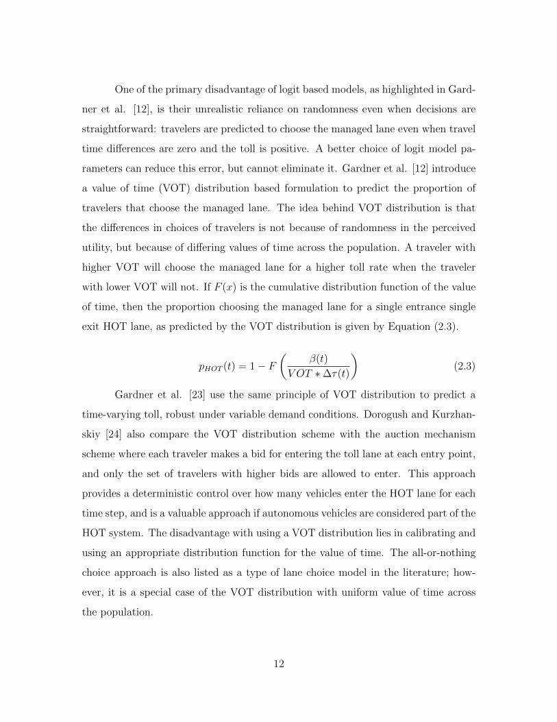
One of the primary disadvantage of logit based models, as highlighted in Gard-

ner et al. [12], is their unrealistic reliance on randomness even when decisions are

straightforward: travelers are predicted to choose the managed lane even when travel

time differences are zero and the toll is positive. A better choice of logit model pa-

rameters can reduce this error, but cannot eliminate it. Gardner et al. [12] introduce

a value of time (VOT) distribution based formulation to predict the proportion of

travelers that choose the managed lane. The idea behind VOT distribution is that

the differences in choices of travelers is not because of randomness in the perceived

utility, but because of differing values of time across the population. A traveler with

higher VOT will choose the managed lane for a higher toll rate when the traveler

with lower VOT will not. If F (x) is the cumulative distribution function of the value

of time, then the proportion choosing the managed lane for a single entrance single

exit HOT lane, as predicted by the VOT distribution is given by Equation (2.3).

pHOT (t) = 1− F(

β(t)

V OT ∗∆τ(t)

)(2.3)

Gardner et al. [23] use the same principle of VOT distribution to predict a

time-varying toll, robust under variable demand conditions. Dorogush and Kurzhan-

skiy [24] also compare the VOT distribution scheme with the auction mechanism

scheme where each traveler makes a bid for entering the toll lane at each entry point,

and only the set of travelers with higher bids are allowed to enter. This approach

provides a deterministic control over how many vehicles enter the HOT lane for each

time step, and is a valuable approach if autonomous vehicles are considered part of the

HOT system. The disadvantage with using a VOT distribution lies in calibrating and

using an appropriate distribution function for the value of time. The all-or-nothing

choice approach is also listed as a type of lane choice model in the literature; how-

ever, it is a special case of the VOT distribution with uniform value of time across

the population.

12

2.2.2 Traffic Flow Model

Traffic flow models can be broadly classified into macroscopic, mesoscopic

and microscopic models, which differ in terms of the resolution of modeling network

features [25]. The primary objective of traffic flow models is to predict the state

of traffic in future time steps, which may then be used to determine the travel time

differences between the HOT and the GP lane. Traffic flow models also predict density

and speed measurements which are used as part of constraints to ensure a minimum

level of service on the HOT lane.

Microscopic models are the ones most commonly used in practice for modeling

HOT lanes. They offer the advantage of capturing vehicle-to-vehicle dynamics in a

detailed manner, especially the lane changing behavior. These include the work by

Cheng and Ishak [26], where a VISSIM model is used to develop feedback based

tolling; Michalaka et al. [27], where a toll pricing comparative model is developed in

CORSIM; and Morgul and Ozbay [19], where a feedback based tolling for a two route

network is developed in Paramics.

Mesoscopic models have also been used predominantly as they are easier to

calibrate and involve fewer traffic state variables. They have been used in computing

optimal tolls for HOT lanes with a single entrance and exit. Lou et al. [3] use a

cell transmission model with lane changing behavior, Gardner et al. [12] use a single

bottleneck pricing model, and Michalaka et al. [2] and Dorogush and Kurzhanskiy

[24] use a modified form of the cell transmission model. The advantage of one model

over the other is often insignificant as each of them provide the needed estimate of

traffic evolution and travel time estimates. To our best knowledge, no literature in

the field of modeling managed lane was found to use macroscopic models. This is

because macroscopic models do not provide the time dependent prediction of traffic

state which is the essential component for determining dynamic tolls.

13

The choice of the traffic flow model also depends on the type of objectives

being used in the toll pricing model, and the HOT system constraints. For example,

the toll pricing model in Leonhardt et al. [28], that aims to maintain a speed limit

on the HOT lane, requires a microsimulation model to predict current speed on the

HOT lanes accurately.

2.2.3 Toll Pricing Model

A toll pricing model determines the choice of toll based on network conditions

(dynamic tolling) or based on a predetermined rate of change. Some of the dynamic

toll pricing models derive tolls based on feedback measurements from the detectors

in real-time (such as Yin and Lou [15]). Other dynamic toll pricing models solve an

optimization problem to determine the optimal tolls. Several objectives have been

considered to determine the optimal toll. The primary ones include:

1. Revenue maximization: The objective here is to maximize the revenue generated

over the total time horizon. Cheng and Ishak [26] develop a feedback-based

revenue maximization method for toll lanes on I-95 in Florida, and utilize the

density, travel time, toll, and speed measurements from previous time step to

determine the toll for the next time step while maintaining a level of service on

the managed lanes. Yang et al. [29] maximize the total expected revenue over

a system of managed lanes with multiple entrances and exits. Goccmen et al.

[18] address the same problem of maximizing the total expected revenue and

compare the performance of adaptive and myopic policies.

2. System throughput maximization: The objective here is to maximize the total

flow out of the system which consists of both the HOT and the GP lane. It is

referred to as the ‘full-utilization’ toll in the literature involving optimal tolling

for single entrance single exit HOT lanes [12, 23]. This is because the objective

of maximizing the throughput is equivalent to utilizing the HOT lane to at its

full, which still ensures that users traverse the freeway in free flow travel time.

14

3. Minimizing unsafe driving behaviors : Lou et al. [3] highlight the importance of

robustness of the toll (toll that do not confuse drivers with sudden updates),

and penalizes lane change behaviors in their objective.

4. Maximizing equity : It is often argued that congestion pricing create equity issues

in a society where rich people pay for shorter travel times. Paleti et al. [30]

develop an income based multi class tolling for a single entrance/exit HOT lane

to balance equity issues.

5. Combined objectives : Many researchers have pointed out the non-uniqueness

of tolls that satisfy a particular objective [31], and in such cases combined

objectives can be used to set the tolls which satisfy multiple criteria.

Most optimization models include a constraint that a minimum level of service

is maintained on the HOT lane. This constraint is modeled differently based on the

type of traffic flow model used. Mesoscopic models, like in Gardner et al. [12] and

Lou et al. [3], which use a triangular or a trapezoidal fundamental diagram, ensure

that the number of travelers entering the HOT lane for each time step is always

below the capacity to guarantee free flow conditions on the HOT lane. Other models

incorporate constraints on the observed density of the freeway. Usually, governments

also regulate the maximum and the minimum toll charged for any particular time

step, and these constraints are also included in these toll setting problems.

Recent literature has also explored alternate ways of charging tolls for HOT

lanes. Laval et al. [31] compare three different pricing strategies for single entrance

single exit HOT lane: tolls that maximize the revenue, pricing scheme with refund

option, and a tradable credit scheme to promote staggered work schedules in firms.

The toll pricing with refund option has also been studied in Lou et al. [32].

15

2.2.4 Demand Model

This component of modeling managed lanes focuses on determining the de-

mand using the HOT lane facility. Though similar demand prediction strategies can

be found in the literature on OD matrix estimation in transportation planning, the

demand model for HOT lanes also involves predicting demand in real-time for the

future time steps, or calibrating the demand distribution. The following key methods

have been used in literature for the demand models:

1. Deterministic demand : Some of the models assume a known demand distribu-

tion at the decision points. These include Gardner et al. [12] and Dorogush

and Kurzhanskiy [24].

2. Stochastic demand with known probability distribution: Most of the stochastic

models use this assumption, e.g. Gardner et al. [23] and Gocmen et al. [18].

The calibration factors in the choice of demand distribution is an area where

further research is needed for such models.

3. Self learning and feedback learning approaches : These approaches do not make

any assumption on the demand and simply utilize the detector readings to

predict or calibrate the lane choice model or the toll pricing model.

4. Demand prediction approaches : These approaches predict the demand in future

using regression models, and is often used when revenue maximizing toll objec-

tive is in place. For example, Toledo et al. [33] use an autoregressive model

to predict the traffic inflow at the entrance of the HOT lane diverge during a

prediction horizon.

2.2.5 Summary Table

Table 2.1 summarizes each of the four models used in literature. This list is

not exhaustive, but is meant to facilitate comparison of these options.

16

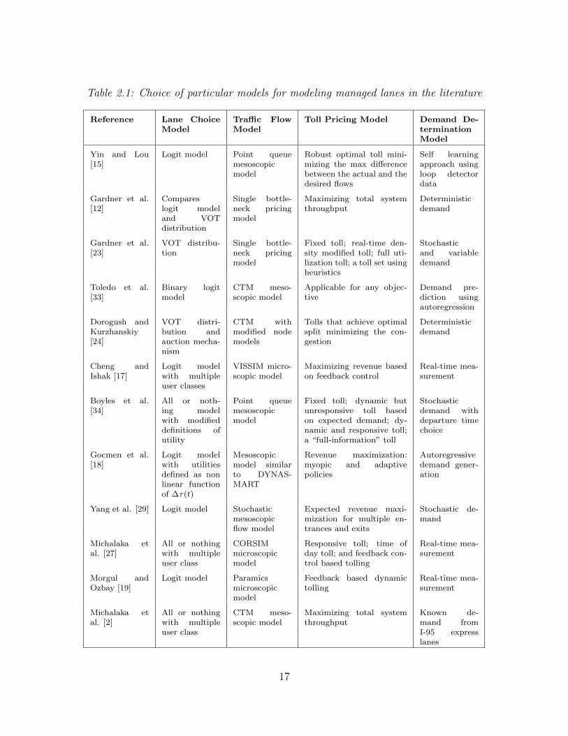
Table 2.1: Choice of particular models for modeling managed lanes in the literature

Reference Lane ChoiceModel

Traffic FlowModel

Toll Pricing Model Demand De-terminationModel

Yin and Lou[15]

Logit model Point queuemesoscopicmodel

Robust optimal toll mini-mizing the max differencebetween the actual and thedesired flows

Self learningapproach usingloop detectordata

Gardner et al.[12]

Compareslogit modeland VOTdistribution

Single bottle-neck pricingmodel

Maximizing total systemthroughput

Deterministicdemand

Gardner et al.[23]

VOT distribu-tion

Single bottle-neck pricingmodel

Fixed toll; real-time den-sity modified toll; full uti-lization toll; a toll set usingheuristics

Stochasticand variabledemand

Toledo et al.[33]

Binary logitmodel

CTM meso-scopic model

Applicable for any objec-tive

Demand pre-diction usingautoregression

Dorogush andKurzhanskiy[24]

VOT distri-bution andauction mecha-nism

CTM withmodified nodemodels

Tolls that achieve optimalsplit minimizing the con-gestion

Deterministicdemand

Cheng andIshak [17]

Logit modelwith multipleuser classes

VISSIM micro-scopic model

Maximizing revenue basedon feedback control

Real-time mea-surement

Boyles et al.[34]

All or noth-ing modelwith modifieddefinitions ofutility

Point queuemesoscopicmodel

Fixed toll; dynamic butunresponsive toll basedon expected demand; dy-namic and responsive toll;a “full-information” toll

Stochasticdemand withdeparture timechoice

Gocmen et al.[18]

Logit modelwith utilitiesdefined as nonlinear functionof ∆τ(t)

Mesoscopicmodel similarto DYNAS-MART

Revenue maximization:myopic and adaptivepolicies

Autoregressivedemand gener-ation

Yang et al. [29] Logit model Stochasticmesoscopicflow model

Expected revenue maxi-mization for multiple en-trances and exits

Stochastic de-mand

Michalaka etal. [27]

All or nothingwith multipleuser class

CORSIMmicroscopicmodel

Responsive toll; time ofday toll; and feedback con-trol based tolling

Real-time mea-surement

Morgul andOzbay [19]

Logit model Paramicsmicroscopicmodel

Feedback based dynamictolling

Real-time mea-surement

Michalaka etal. [2]

All or nothingwith multipleuser class

CTM meso-scopic model

Maximizing total systemthroughput

Known de-mand fromI-95 expresslanes

17

2.3 Data Requirements

Loop detector data is one of the most readily available data sources used for

calibrating and validating models. Loop detectors can provide an estimate of the

speed with which vehicles travel, the occupancy rate (which is a proxy for density),

and the count of the number of vehicles traveling across them. There are two primary

uses of the loop detector data in the literature:

Using the data collected in the past: The objective here is to mine the

loop detector data to extract meaningful information about the driver behavior or

factors affecting the managed lane model. Abdel et al. [35] use loop detector data

collected on a 13.25 mile stretch on I-4 in Florida and correlate it with the crash

reports to develop a crash likelihood prediction model for identifying the locations

to be flagged as a potential crash locations. Liu et al. [21] use loop detector data

to determine the time dependent values for the value of time (VOT) and the value

of reliability (VOR), which is one example of the usage of loop detector data for

revealed preference studies. Kwon et al. [36] use loop detector data to build travel

time trends and regression models for predicting future travel times. PeMS, the

freeway Performance Monitoring System, developed for the California Department

of Transportation, also reports the traffic conditions in real-time by mining the loop

detector data for traffic operations and planning [37]. Most of these researches point

out the effort required to remove the erroneous loop detector readings before they are

used in the planning models.

Using the data collected in real time: The objective here is to use the

data that is being collected in real time to develop or calibrate models online and

use instantly. Most of the feedback based controls rely on the online data. These

include deciding the controls for ATM strategies like variable speed limits, ramp

metering, dynamic lane use control etc., which are widely in use across United States

and Europe [38]. Feedback based controls have been used in developing heuristic

18

pricing strategies for the HOT lanes and are often widely incorporated in practice.

Yin and Lou [15] and Cheng and Ishak [17] develop simulations using the real-time

loop detector readings to develop feedback based control for HOT pricing.

However, using such data in real time involves accounting for errors due to

faulty detection or external factors. Models for optimal pricing for HOT lane using

real-time loop detector data have been studied in Lou et al.[3] and Michalaka et

al.[16]. Both these studies assume that the error in the formulation involving the

loop detector readings has a gaussian distribution with a known mean and variance.

Some researchers have attempted to look at the type of errors generated by

the loop detectors and suggested ways to correct them. Li et al. [39] study the errors

generated by loop detector data collected for 99 intersections in Changsha, China,

and point out that these errors depend on the type of lane and the intersection

size. A sample error plot for the density observations from loop detector data is

shown to have a peak around zero with flattening tails in both positive and negative

direction, which resembles a gaussian distribution. Jacobson et al. [40] point out the

importance of detecting erroneous data and develop a test involving the predicted

volume-to-occupancy ratio to identify detector malfunctions. Bie et al. [41] develop

a diagnosis method and an imputation method to detect and fill missing or erroneous

data in real-time loop detector readings.

2.4 Modeling Managed Lanes Corridor with Multiple En-

trances and Exits

Most research on optimal pricing for HOT lanes has focused on networks with

single entrances and exits. These networks are much simpler: the decision of whether

to choose the HOT lane is made at only one decision point. For HOT lane networks

with multiple entrances and exits, the number of decision points increase which creates

further complications in the modeling process (explained in more detail in Chapter

19

4).

Very few researchers have attempted to address the pricing problem for HOT

networks beyond a single entrance and exit, with a few exceptions:

Michalaka et al. [27] develop a simulation based evaluation model for different

tolling strategies for I-95 express lanes in Florida with multiple entrances and exits.

In particular, four tolling strategies are evaluated: zone based tolling, origin specific

tolling, OD based tolling, and distance based tolling. However, they assume a fixed

toll rate for each of the strategy, and no optimization of the toll pricing is done.

Dorogush and Kurzhanskiy [24] propose a model in which a regular lane is

converted into a HOT lane based on the prevailing traffic conditions. They determine

a desired optimal split at each diverge point based on the traffic conditions, and then

set the tolls to achieve that split. The demand is assumed deterministic in their case.

It is, however, challenging to extend their models for HOT lane systems in practice,

where a separate lane is marked and barricaded for the HOT use.

Song et al. [42] address the issue of determining optimal locations for con-

verting HOV lanes into HOT lanes in a general network, and simultaneously develop

optimal toll pricing which maximizes net social benefit. They formulate the prob-

lem as a MPCC (mathematical program with complementarity constraints) assuming

that the network is time-independent and the travel time on each link can be ex-

pressed as analytical functions of the flow variable. However, the assumption of time

independency of the network is restrictive for it to be applied on real networks.

Yang et al. [29] develop a distance based tolling model for a HOT network

with multiple entrance and exits with revenue maximization as the primary objective.

They make a simplifying assumption that the traffic flow on the GP lane is not affected

by the travelers shifting to the HOT lane, and thus travel time on the GP lane is

independent of the toll prices. Also, it is assumed that a traveler makes the choice

20

of entering the managed lane only once, and after taking the HOT lane the traveler

will not leave the HOT lane until the exit point has been reached. With additional

assumptions, the problem is reduced to a stochastic dynamic programming problem

which is solved on a network with three entrances and a single exit to develop an

approximate optimal price that maximizes the expected revenue.

Chapters 4 and 5 of this thesis attempt to fill the gaps in the literature by

formulating the problem without making the assumptions made in Yang et al. [29],

and developing the formulation in discrete time which is more useful from a practical

standpoint.

2.5 Summary

This chapter provides an overview of the existing literature in the field of

managed lane pricing and the current trends of dynamic pricing in United States. As

observed, commonly used methods for dynamic pricing in practice involve feedback

based control and heuristic algorithms in which predetermined thresholds are used to

determine the decision of increasing or decreasing the toll. These algorithms have a

scope of improvement.

Managed lane models have four primary components: lane choice model; traffic

flow model; toll pricing model; and demand model. Several researchers have used

logit models for modeling choice between the HOT and the GP lane. They are

easier to use but suffer from the disadvantage of making unreasonable predictions

of split proportions [12]. VOT distribution method is more realistic, but the choice

of an appropriate distribution is harder to obtain. Chapter 3 attempts to develop

an estimation model for the parameters of VOT distribution using real-time loop

detector data.

Regarding the choice of traffic flow models, microscopic traffic models have

been found more reasonable as they capture the vehicle-to-vehicle interaction and

21

the lane choice behaviors at diverge points. However, given the simplicity to use the

mesoscopic models in formulation of optimal dynamic tolls, they are considered in

the formulations developed in this thesis.

Among different toll pricing objectives, revenue maximization and total system

travel time minimization are the most commonly used objectives in practice and are

considered for the models in Chapters 3, 4 and 5. In demand models, it is either

assumed that a probability distribution for the demand is known or the demand

is predicted based on the real-time or previously collected loop detector data. In

Chapter 3, the real-time loop detector data is used to replace a known value for the

demand. In Chapters 4 and 5, a deterministic demand assumption is made to simplify

the modeling efforts which will be relaxed as part of the future work.

For using real-time measurements in estimation or optimal pricing, previous

work has emphasized on the methods which address measurement errors due to de-

tector malfunctions [39, 40, 41]. An appropriate choice for the error distribution is

also important for developing an accurate estimation model.

More research needs to be done in understanding how real-time loop detector

data can be used for developing optimal HOT tolls, and for HOT lane networks with

multiple entrances and exits. This thesis seeks to address these problems in greater

detail.

22

Chapter 3

Estimation for Single Entrance Single Exit

Managed Lane

This chapter introduces a method for using the real-time loop detector data

to estimate the users’ willingness to pay, and to set the optimal tolls for a HOT

network with a single entrance and exit. This method fits in the broader context

of determining optimal tolls for complex HOT networks using real-time data, and

lays the foundation for estimation and optimization of dynamic tolls (referred to as

self-learning approach in literature).

We assume that a value of time (VOT) distribution is used to model the lane

choice behavior of the travelers and use link transmission model (LTM) (which is a

mesoscopic traffic flow model proposed by Yperman [43]) to update the traffic flow

with time. The toll pricing objective considered in the model is to maximize the

throughput through a HOT-SESE network. The demand is assumed to be unknown

and the modeling relies only on the self-learning approach and loop detector data.

3.1 Background

Knowing the VOT distribution is essential to set tolls that achieve a particular

objective, like minimizing total system travel time [12]. Most commonly used methods

to predict the VOT distribution for a population involve revealed preference surveys

or a projection based on the income distribution of the population [44, 12].

The proposed method in this chapter uses loop detector data to estimate the

VOT distribution parameters. The reason behind using the loop detector data is

23

that the measured number of vehicles choosing the HOT lane and the GP lane for a

given value of the toll and the travel time difference between the two lanes can help

in predicting the true parameters of VOT for the population using the HOT system.

However, loop detector data are associated with measurement errors. Common

sources of error include magnetic field disturbance from external objects other than

the vehicles and temperature changes around the detector. The reliability of such

measurements is thus often questionable. However, if we assume that the error is

of a particular form, we can use probabilistic estimation theory to predict the VOT

distribution parameters from the measurements.

Many different form of VOT distribution have been proposed in the literature.

Ben Akiva et al. [45] suggest that the VOT follows a log-normal distribution. Burr

distribution, as proposed in Gardner et al. [12], is commonly used to model the income

of a population, and is assumed to reflect the distribution of the VOT. The cumulative

distribution function for the Burr distribution is given by Equation (3.1) and is easier

to work with, as compared to the cumulative distribution of the log-normal function.

F

(β(t)

∆τ(t), ζ, γ

)= 1− 1

1 +(

β(t)ζ∆τ(t)

)γ (3.1)

where β(t) refers to the toll charged for time step t and ∆τ(t) is the travel time

difference between the two lanes. The cumulative distribution function in (3.1) can

be substituted in Equation (2.3) to get the value of pHOT (t) which is the proportion

of travelers choosing the HOT lane at time step t.

In Equation (3.1), the parameters ζ and γ are often unknown and vary for

the population. The primary idea of this chapter is to utilize the loop detector data

to estimate the values of these variables on any particular day of the operation of

managed lanes.

24

3.2 Estimation and Toll Optimization in Real Time

The proposed model borrows the reactive learning approach proposed in Lou et

al. [3], in which the loop detector data is used to estimate the logit model parameters.

This section addresses the same problem using the VOT distribution. We assume that

the VOT distribution follows the Burr distribution as in Equation (3.1). A single

entrance single exit HOT lane network is considered, and a downstream bottleneck

is assumed to be located for the general-purpose (GP) lane to model congestion.

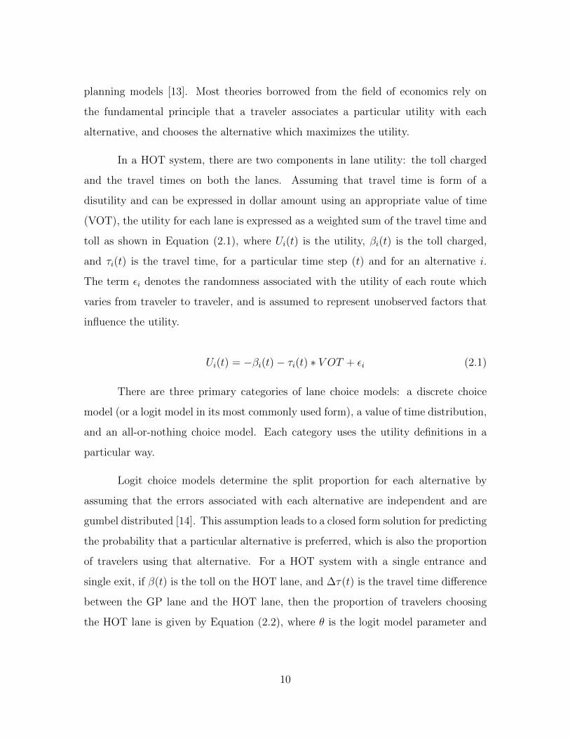
3.2.1 Notations

Consider the HOT-SESE system shown in Figure 3.1, which shows the lo-

cation of four loop detectors installed upstream and downstream of the toll gantry

point on each of the HOT and the GP lane. The variables µR(t), µT (t), λR(t), and

λT (t) represent the loop detector readings for the corresponding detector locations,

evaluated as the number of travelers passing through the detector for time step t.

ζ and γ are the burr distribution parameters that need to be estimated, and ζ and

γ represent the current estimated value of those parameters, respectively. The toll

rate at the start of time step t is represented as β(t) and the travel time difference

between the GP and the HOT lane at the start of time step t is represented as ∆τ(t).

The simulation horizon is represented by a set of discrete time steps t defined as a set

of non-negative integers with maximum value as T representing the last time step of

the simulation. The current time step is represented as tc. Table 3.1 summarizes the

notations used in the estimation model.

25

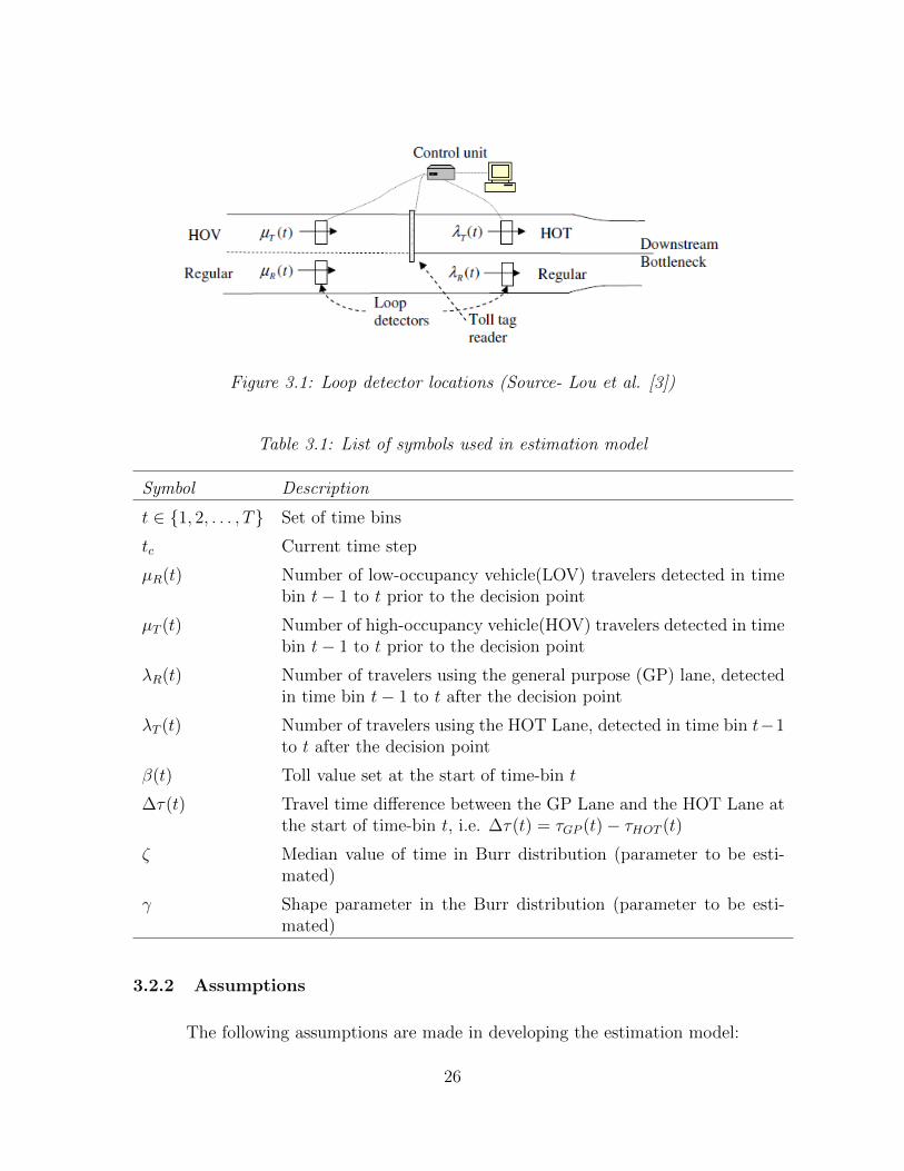
Figure 3.1: Loop detector locations (Source- Lou et al. [3])

Table 3.1: List of symbols used in estimation model

Symbol Description

t ∈ {1, 2, . . . , T} Set of time bins

tc Current time step

µR(t) Number of low-occupancy vehicle(LOV) travelers detected in timebin t− 1 to t prior to the decision point

µT (t) Number of high-occupancy vehicle(HOV) travelers detected in timebin t− 1 to t prior to the decision point

λR(t) Number of travelers using the general purpose (GP) lane, detectedin time bin t− 1 to t after the decision point

λT (t) Number of travelers using the HOT Lane, detected in time bin t−1to t after the decision point

β(t) Toll value set at the start of time-bin t

∆τ(t) Travel time difference between the GP Lane and the HOT Lane atthe start of time-bin t, i.e. ∆τ(t) = τGP (t)− τHOT (t)

ζ Median value of time in Burr distribution (parameter to be esti-mated)

γ Shape parameter in the Burr distribution (parameter to be esti-mated)

3.2.2 Assumptions

The following assumptions are made in developing the estimation model:

26

1. Travelers approaching the managed lane prior to the decision point segregate

in a manner that µR(t) accounts for all the low-occupancy vehicles (LOV), and

µT (t) accounts for all the high-occupancy vehicles (HOV). Such an assumption

is simply to ensure that the split of the LOV and the HOV vehicles in the

approaching demand is known, which is usually the case as the HOVs need to

notify the system that they will be traveling through the network.

2. All HOVs always choose the managed lane. This assumption is reasonable as

there is no toll for the high-occupancy vehicles on the HOT lane.

3. All travelers detected in µR(t) and µT (t), make the decision during the time

interval t to t + 1, and are detected by the detectors located after the decision

point in the same time step. That is, µR(t) + µT (t) = λR(t) + λT (t) for all

t, without including the error term in each detector reading. This assumption

is reasonable if the detectors are located close to each other. However, it is

not restrictive because based on the distance between the detectors, a time lag

parameter can be introduced which ensures that upstream detector readings

sum up to the downstream detector readings after a time lag.

4. The errors in the loop detector data are assumed independent, both spatially

and over time.

3.2.3 Estimation Model

The estimation model uses the method of batch least squares to perform non-

linear estimation of the VOT distribution parameters. Each of the loop detector

readings come with an associated error εi, where i refers to the i-th loop detector. As

observed in Li et al. [39], these errors tend to have a distribution approximately close

to a gaussian distribution. The proportion of travelers choosing the HOT lane at each

time step can then be expressed in terms of the VOT parameters to be estimated for

27

each time step.

pHOT (t) =1

1 +

(β(t)

ζ∆τ(t)

)γ (3.2)

λT (t) + ελT − µT (t)− εµTµR(t) + εµR

=1

1 +

(β(t)

ζ∆τ(t)

)γ (3.3)

µR(t) + εµRλT (t) + ελT − µT (t)− εµT

− 1 =

(β(t)

ζ∆τ(t)

)γ(3.4)

log

(µR(t) + εµR

λT (t) + ελT − µT (t)− εµT− 1

)= γ

(log(

β(t)

∆τ(t))− log(ζ)

)(3.5)

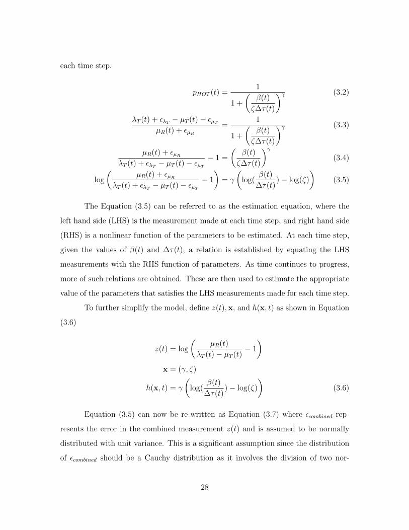
The Equation (3.5) can be referred to as the estimation equation, where the

left hand side (LHS) is the measurement made at each time step, and right hand side

(RHS) is a nonlinear function of the parameters to be estimated. At each time step,

given the values of β(t) and ∆τ(t), a relation is established by equating the LHS

measurements with the RHS function of parameters. As time continues to progress,

more of such relations are obtained. These are then used to estimate the appropriate

value of the parameters that satisfies the LHS measurements made for each time step.

To further simplify the model, define z(t),x, and h(x, t) as shown in Equation

(3.6)

z(t) = log

(µR(t)

λT (t)− µT (t)− 1

)x = (γ, ζ)

h(x, t) = γ

(log(

β(t)

∆τ(t))− log(ζ)

)(3.6)

Equation (3.5) can now be re-written as Equation (3.7) where εcombined rep-

resents the error in the combined measurement z(t) and is assumed to be normally

distributed with unit variance. This is a significant assumption since the distribution

of εcombined should be a Cauchy distribution as it involves the division of two nor-

28

mally distributed random variables. However, such a simplification allows the use of

standard algorithms to determine the parameters.

z(t) = h(x, t) + εcombined (3.7)

Given these assumptions, we can run a batch least squares method to estimate

the parameters x given the measurement made at each time step. The objective used

to determine x minimizes the least squares of the errors generated by the estimated

values as shown in Equation (3.8), where z is the column matrix of all z(t) and h(x)

is the column matrix of all h(x, t) for all t ≤ tc. The objective considers all data

points upto time t ≤ tc and hence determines newer values of x as time progresses.

x = argminx

Jc(x) = argminx||z − h(x)||2 (3.8)

The Gauss-Newton estimation algorithm (Algorithm 1) was used to solve the

non-linear estimation problem. The algorithm solves the optimization problem by

starting with a initial guess of the parameter values, and determines the direction of

descent (∆x) at each point. This determination is based on linearizing the derivative

of the Jc(x) at the current guess and finding a value of ∆x which sets this linearized

derivative to 0. This linearization assumes that the residual errors (z − h(x)) are

small, ignoring the higher order terms. It then determines the step size α to be taken

in the direction of descent (∆x) such that the objective function reduces after every

step. More details about the derivation of this algorithm can be found in standard

non-linear estimation texts (see Bar-Shalom et al. [46]).

29

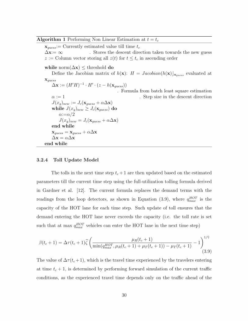
Algorithm 1 Performing Non Linear Estimation at t = tc

xguess:= Currently estimated value till time tc∆x:= ∞ . Stores the descent direction taken towards the new guessz := Column vector storing all z(t) for t ≤ tc in ascending order

while norm(∆x) ≤ threshold doDefine the Jacobian matrix of h(x): H = Jacobian(h(x)cxguess evaluated at

xguess∆x := (H ′H)−1 ·H ′ · (z − h(xguess))

. Formula from batch least square estimationα := 1 . Step size in the descent directionJ(xg)new := Jc(xguess + α∆x)while J(xg)new ≥ Jc(xguess) do

α:=α/2J(xg)new = Jc(xguess + α∆x)

end whilexguess = xguess + α∆x∆x = α∆x

end while

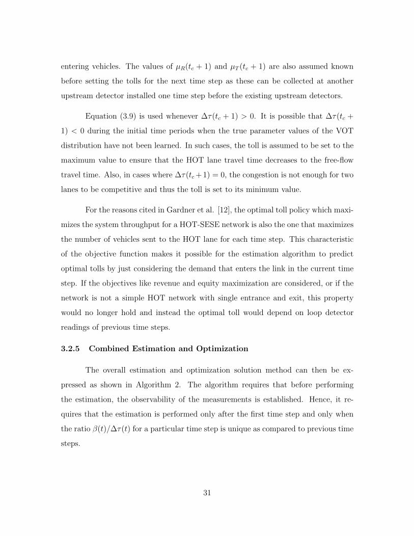
3.2.4 Toll Update Model

The tolls in the next time step tc + 1 are then updated based on the estimated

parameters till the current time step using the full-utilization tolling formula derived

in Gardner et al. [12]. The current formula replaces the demand terms with the

readings from the loop detectors, as shown in Equation (3.9), where qHOTmax is the

capacity of the HOT lane for each time step. Such update of toll ensures that the

demand entering the HOT lane never exceeds the capacity (i.e. the toll rate is set

such that at max qHOTmax vehicles can enter the HOT lane in the next time step)

β(tc + 1) = ∆τ(tc + 1)ζ

(µR(tc + 1)

min(qHOTmax , µR(tc + 1) + µT (tc + 1))− µT (tc + 1)− 1

)1/γ

(3.9)

The value of ∆τ(tc+1), which is the travel time experienced by the travelers entering

at time tc + 1, is determined by performing forward simulation of the current traffic

conditions, as the experienced travel time depends only on the traffic ahead of the

30

entering vehicles. The values of µR(tc + 1) and µT (tc + 1) are also assumed known

before setting the tolls for the next time step as these can be collected at another

upstream detector installed one time step before the existing upstream detectors.

Equation (3.9) is used whenever ∆τ(tc + 1) > 0. It is possible that ∆τ(tc +

1) < 0 during the initial time periods when the true parameter values of the VOT

distribution have not been learned. In such cases, the toll is assumed to be set to the

maximum value to ensure that the HOT lane travel time decreases to the free-flow

travel time. Also, in cases where ∆τ(tc+ 1) = 0, the congestion is not enough for two

lanes to be competitive and thus the toll is set to its minimum value.

For the reasons cited in Gardner et al. [12], the optimal toll policy which maxi-

mizes the system throughput for a HOT-SESE network is also the one that maximizes

the number of vehicles sent to the HOT lane for each time step. This characteristic

of the objective function makes it possible for the estimation algorithm to predict

optimal tolls by just considering the demand that enters the link in the current time

step. If the objectives like revenue and equity maximization are considered, or if the

network is not a simple HOT network with single entrance and exit, this property

would no longer hold and instead the optimal toll would depend on loop detector

readings of previous time steps.

3.2.5 Combined Estimation and Optimization

The overall estimation and optimization solution method can then be ex-

pressed as shown in Algorithm 2. The algorithm requires that before performing

the estimation, the observability of the measurements is established. Hence, it re-

quires that the estimation is performed only after the first time step and only when

the ratio β(t)/∆τ(t) for a particular time step is unique as compared to previous time

steps.

31

Algorithm 2 Estimation and Optimization

Set tc = 0 and β(0) = βminInitialize the value of parameters (γ0 and ζ0)while tc < T do

Collect loop detector readings for time step tc

Estimate:Use Loop detector readings to perform estimation if t ≥ 2, ∆τ > 0,and β(t)/∆τ(t) is unique

Forward Simulate: Use forward simulation with the LTM traffic flow modelto determine the experienced travel times for the next time step

Toll update: Use the latest estimated values of the parameters and the traveltimes for the next time step to determine the optimal toll using Equation (3.9)

if β(tc + 1) > βmax OR β(tc + 1) < βmin thenSet β(tc + 1) to the appropriate boundary value

end ifif τHOT (t) > ffHOT then

Set β(tc + 1) to βmaxend ifif ∆τ(t) = 0 then

Set β(tc + 1) to βminend ifSet tc = tc + 1

end while

3.3 Simulation and Results

To test the performance of the proposed estimation and optimization algo-

rithm, Algorithm 2 was coded in Matlab, and a simulation study was conducted with

artificially generated demand for a simple network with single entrance and exit. A

10 km corridor was simulated with three GP lanes, each with the capacity of 2100

veh/hr, and one HOT lane with capacity 1800 veh/hr. The downstream bottleneck

was assumed to reduce the capacity of GP lane from three lanes to two lanes. The

free-flow speed was assumed as 100km/hr on both the lanes. The demand values used

in the simulation are shown in Table 3.2 in units of veh/hr.

32

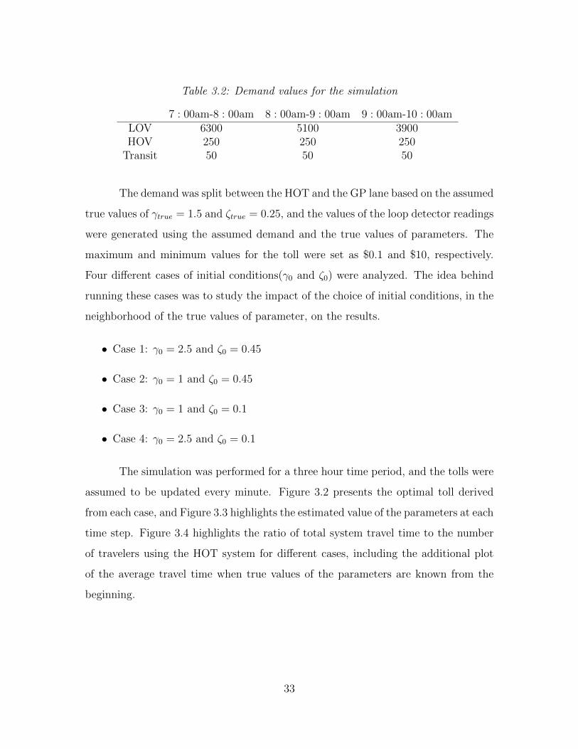
Table 3.2: Demand values for the simulation

7 : 00am-8 : 00am 8 : 00am-9 : 00am 9 : 00am-10 : 00amLOV 6300 5100 3900HOV 250 250 250

Transit 50 50 50

The demand was split between the HOT and the GP lane based on the assumed

true values of γtrue = 1.5 and ζtrue = 0.25, and the values of the loop detector readings

were generated using the assumed demand and the true values of parameters. The

maximum and minimum values for the toll were set as $0.1 and $10, respectively.

Four different cases of initial conditions(γ0 and ζ0) were analyzed. The idea behind

running these cases was to study the impact of the choice of initial conditions, in the

neighborhood of the true values of parameter, on the results.

• Case 1: γ0 = 2.5 and ζ0 = 0.45

• Case 2: γ0 = 1 and ζ0 = 0.45

• Case 3: γ0 = 1 and ζ0 = 0.1

• Case 4: γ0 = 2.5 and ζ0 = 0.1

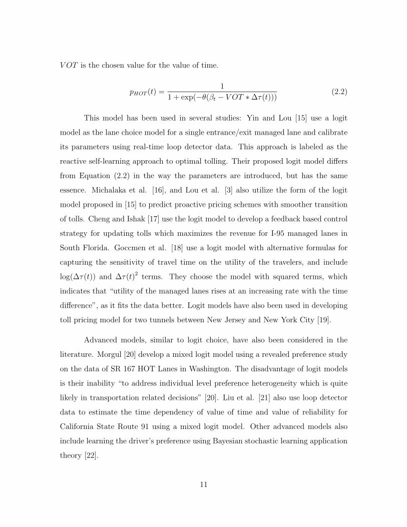
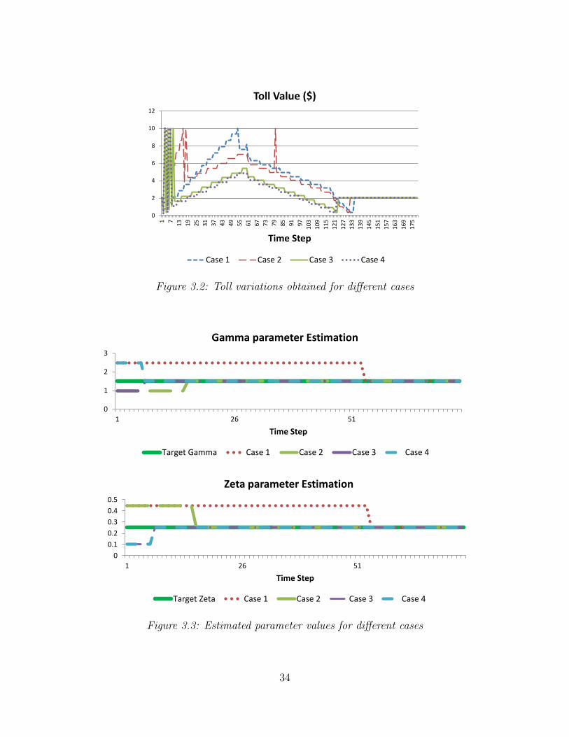
The simulation was performed for a three hour time period, and the tolls were

assumed to be updated every minute. Figure 3.2 presents the optimal toll derived

from each case, and Figure 3.3 highlights the estimated value of the parameters at each

time step. Figure 3.4 highlights the ratio of total system travel time to the number

of travelers using the HOT system for different cases, including the additional plot

of the average travel time when true values of the parameters are known from the

beginning.

33

0

2

4

6

8

10

12

1 7

13

19

25

31

37

43

49

55

61

67

73

79

85

91

97

10

3

10

9

11

5

12

1

12

7

13

3

13

9

14

5

15

1

15

7

16

3

16

9

17

5

Time Step

Toll Value ($)

Case 1 Case 2 Case 3 Case 4

Figure 3.2: Toll variations obtained for different cases

0

1

2

3

1 26 51

Time Step

Gamma parameter Estimation

Target Gamma Case 1 Case 2 Case 3 Case 4

0

0.1

0.2

0.3

0.4

0.5

1 26 51

Time Step

Zeta parameter Estimation

Target Zeta Case 1 Case 2 Case 3 Case 4

Figure 3.3: Estimated parameter values for different cases

34

0

2

4

6

8

10

12

Case1 Case2 Case3 Case4 TRUE

Avg. Corridor Travel Time per Traveler (min)

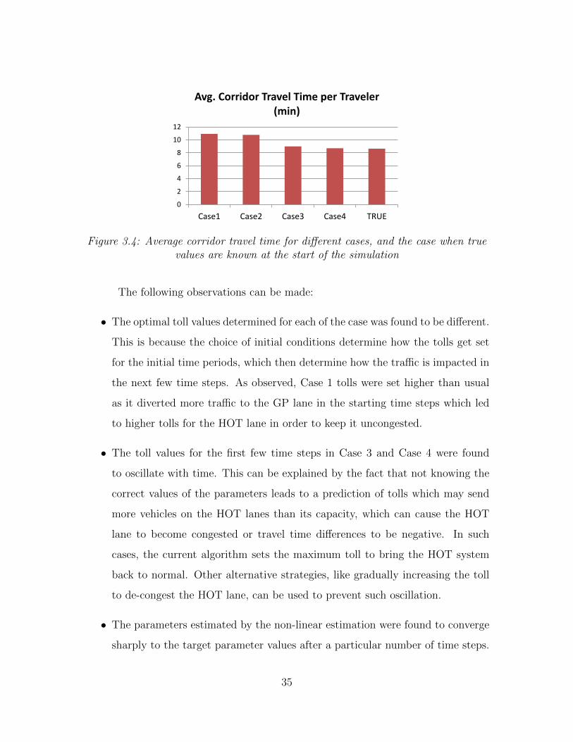
Figure 3.4: Average corridor travel time for different cases, and the case when truevalues are known at the start of the simulation

The following observations can be made:

• The optimal toll values determined for each of the case was found to be different.

This is because the choice of initial conditions determine how the tolls get set

for the initial time periods, which then determine how the traffic is impacted in

the next few time steps. As observed, Case 1 tolls were set higher than usual

as it diverted more traffic to the GP lane in the starting time steps which led

to higher tolls for the HOT lane in order to keep it uncongested.

• The toll values for the first few time steps in Case 3 and Case 4 were found

to oscillate with time. This can be explained by the fact that not knowing the

correct values of the parameters leads to a prediction of tolls which may send

more vehicles on the HOT lanes than its capacity, which can cause the HOT

lane to become congested or travel time differences to be negative. In such

cases, the current algorithm sets the maximum toll to bring the HOT system

back to normal. Other alternative strategies, like gradually increasing the toll

to de-congest the HOT lane, can be used to prevent such oscillation.

• The parameters estimated by the non-linear estimation were found to converge

sharply to the target parameter values after a particular number of time steps.

35

The convergence was found to happen earlier for Cases 2, 3 and 4, but at a later

time step for the Case 1. This sharp convergence and the particular location of

this time step can be explained by the observability of the estimation algorithm.

An observable estimation is made at a time step when enough information has

been collected in form of the unique values of the ratio of β(t) and ∆τ(t).

Since the assumed demand distribution is very monotonic for first few time

steps, unless the toll values are set to a different value as predicted by Equation

(3.9), the system of measurements won’t be observable enough to estimate the

parameters. This explains why Case 1 converges at a later time step than other

cases.

• The average corridor travel time per traveler was found to be lower for the

cases where the convergence of the estimated parameters happened in earlier

time steps. This is because the earlier the parameters converge to the true

value, the earlier the tolls behave optimally. It also indicates that the choice of

initial values of parameters determine the proximity to the optimal solution in

systems where observable measurements are hard to develop.

3.4 Summary

In this chapter, the estimation model developed in Lou et al. [3] was extended

to estimate the parameters of the value of time distribution from the real-time loop

detector data. Maximizing total system throughput was used as the objective for the

optimal tolls. Burr distribution was used to model VOT; however, the methodology

developed is agnostic to the choice of VOT distribution as it utilizes non linear esti-

mation to predict the true values of the parameters. As observed from the simulation

runs on a HOT-SESE network, the choice of initial conditions affect the toll policy

significantly; however, the convergence of the estimated values of the parameters to

their true values was found to happen regardless of the initial conditions. The ob-

servability of the collected measurements was identified as the primary factor that

36

affects the convergence to the true value. In practice, the loop detector readings will

typically not be constant for several time steps, and thus earlier convergence can be

achieved.

The analysis in this chapter provides a background for using the real-time

measurements and computing the toll policies, without relying on basic heuristics

which maybe sub-optimal. This analysis needs to be extended to deal with more

complex HOT networks and other optimization objectives, which will be explored in

the future.

37

Chapter 4

Problem Formulation for Multiple

Entrance Multiple Exit HOT Lanes

This chapter introduces the theory behind optimal pricing for a HOT lane

network with multiple entrances and exits (HOT-MEME), formulates a discrete op-

timization problem for revenue maximization and total system travel time (TSTT)

minimization as the objectives, and proposes a dynamic programming approach to

solve the optimization problem under deterministic demand conditions. The proposed

model provides a background for future extensions into cases of stochastic demand or

demand prediction using real time data collection.

4.1 Characteristics of HOT lanes with Multiple Entrances

and Exits

Consider the abstract HOT-MEME network as shown in the Figure 4.1. The

network represents a system with a HOT lane (the top route) parallel to a general

purpose (GP) lane (the bottom route) connected via ramps at multiple entry/exit

points. A vehicle traveling from node 1 to node 0 has multiple decision points in

between. These decision points are located at each diverge node (nodes 2, 3, 5 and 7).

In contrast to the assumptions made in the previous literature, a traveler can choose

to change their decision at any of the downstream decision point, which makes this a

more general framework for toll optimization on a HOT-MEME network.

38

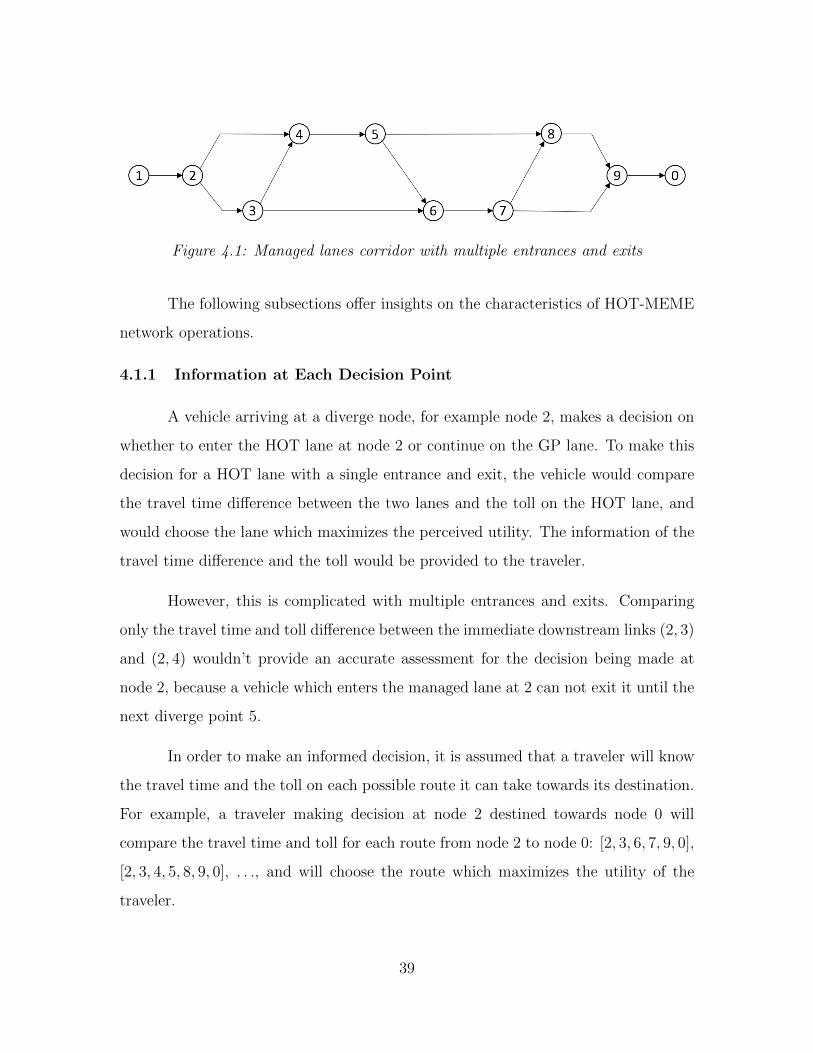
Figure 4.1: Managed lanes corridor with multiple entrances and exits

The following subsections offer insights on the characteristics of HOT-MEME

network operations.

4.1.1 Information at Each Decision Point

A vehicle arriving at a diverge node, for example node 2, makes a decision on

whether to enter the HOT lane at node 2 or continue on the GP lane. To make this

decision for a HOT lane with a single entrance and exit, the vehicle would compare

the travel time difference between the two lanes and the toll on the HOT lane, and

would choose the lane which maximizes the perceived utility. The information of the

travel time difference and the toll would be provided to the traveler.

However, this is complicated with multiple entrances and exits. Comparing

only the travel time and toll difference between the immediate downstream links (2, 3)

and (2, 4) wouldn’t provide an accurate assessment for the decision being made at

node 2, because a vehicle which enters the managed lane at 2 can not exit it until the

next diverge point 5.

In order to make an informed decision, it is assumed that a traveler will know

the travel time and the toll on each possible route it can take towards its destination.

For example, a traveler making decision at node 2 destined towards node 0 will

compare the travel time and toll for each route from node 2 to node 0: [2, 3, 6, 7, 9, 0],

[2, 3, 4, 5, 8, 9, 0], . . ., and will choose the route which maximizes the utility of the

traveler.

39

A challenge with this assumption is that the amount of information presented

to a traveler would be enormous, which might be overwhelming. However, a possible

way to implement this would be to exploit vehicle to-infrastructure (V2I) communi-

cation technologies where the HOT lane system would report all this information to

a traveler inside a vehicle and an external application will then compare the utilities

for each of the route to make the decision for the traveler.

4.1.2 En-route vs Fixed Decision Making

The tolls on the HOT lane change with time and travelers do not know what

the toll would be in the next time step as the tolls are regulated by a central authority.

With this dynamic nature of the toll update, a rational decision for a traveler would

not be to travel on the chosen path until the destination is reached, irrespective of

how tolls change in future time step.

Hence, it is assumed that a traveler will make en-route decisions at every

decision point based on the current prevalent toll rate. It is possible that drivers

may anticipate the toll rate in the future based on their experience, but this calls for

a more complicated game theoretic behavior, and is not considered as part of this

study.

4.1.3 Toll Policy

HOT lanes with multiple entrances and exits can have different toll policies

which determine how a traveler is expected to pay a toll when the rates change with

time. Some of the commonly used ones, as proposed in Michalaka et al. [27], are as

follows:

• Origin based tolling: Here a vehicle pays different toll for entering the HOT

lane from different origins (or entry points). However, the same toll rate applies

regardless of whichever exit point is used.

40

• Origin-destination tolling: Here a vehicle pays a particular toll determined dif-

ferently for each origin-destination (or entry/exit) pair for the HOT lane.

• Distance based tolling: Here a vehicle pays the toll equal to the toll rate at the

instant multiplied with the distance it travels on the HOT lane.

• Zone based tolling: Here a vehicle pays same toll for entering at any origin (or

entry point) in the same zone, but pays a different toll for a different zone for

the HOT lane system.

Distance based tolling is taken to be the focus of this research. Since toll rates

change with time, the most fair way to charge tolls would be to charge each vehicle

the rate it saw while making the decision. This can be easily enforced using the

unique RFID readings from toll tags attached to each vehicle which can record when

a vehicle entered the HOT lane and charge the rate prevalent at that time.

4.1.4 Reporting Instantaneous vs Experienced Travel Times

Experienced travel times are easier to report in HOT lanes with single entrance

and exit. However, for HOT-MEME networks, drivers’ decisions in the future depend

on the future toll rate, and so the travel time experienced by the traveler can not be

predicted with full certainty.

It is thus assumed that travelers compare the instantaneous travel time on

each route. The instantaneous travel time on a route is calculated by adding the

current travel time on each link in the route. Alternative methods for travel time

prediction will be studied as part of the future research.

4.2 Optimization Problem

The goal of this section is to propose a formulation for how the tolls should

be varied with time, so that a particular objective is achieved. In particular, two ob-

jectives are considered in parallel: maximizing revenue, and minimizing total system

41

travel time.

4.2.1 Notations

Table 4.1 lists the notation used in the modeling. Sets N and A represent the

set of all nodes and links in the network, respectively. A link (i, j) belonging to set A

has its tail at node i and its head at node j. Sets Γ−1i and Γi, for a particular node i,

represent the set of all incoming and outgoing links for the node, respectively. These

notations define the connection between nodes and links in the network.

Set A is further decomposed into two disjoint sets AHOT and AGP , which

represent the set of all links which are part of the HOT lane and set of all links

which are not part of the HOT lane, respectively. For the network in Figure 4.1,

AHOT = {(2, 4), (4, 5), (5, 8), (8, 9)}. A binary variable δij is defined for each link

representing whether the link belongs to AHOT or AGP . It takes a value of 1 if the

link belongs to the HOT lane, and 0 otherwise. The toll rate per mile on the HOT

lane as function of time is represented as β(t).

The parameters for a link, used in the mesoscopic traffic flow model, are defined

similar to the previous literature. These include the capacity (qijmax), the jam density

(kijj ), the free-flow speed (uijf ), the backwave speed (wij), and the length (lij) for each

link. The flow on each link is denoted by the sending flow (Sij(t)) and the receiving

flow (Rij(t)), which represent the maximum flow that a link can send and receive in

each time step. yijkj (t) is defined as the transition flow from link (i, j) to (j, k) for

time step t, and represents the actual flow that gets to move from one link to the

other. The cumulative vehicle count at the upstream and the downstream end of a

link (i, j) is represented by variables N↑ij(t) and N↓ij(t) respectively.

The simulation horizon is represented by a set of discrete time steps t defined

as a set of non-negative integers with maximum value as T representing the last time

step of the simulation. The demand originating from an origin r is denoted by dr(t).

42

Table 4.1: List of symbols for the optimization problem

Symbol Description

t ∈ {0, 1, 2, . . . , T} Set of all time steps, each ∆t long

AGP Set of all links which are not part of the HOT lane (or are generalpurpose lanes)

AHOT Set of all links which are part of the HOT lane

(i, j) ∈ A Set of all links in the network (A = AGP ∪ AHOT )

i ∈ N Set of all nodes in the network

qijmax, kijj , u

ijf , wij, lij Capacity, jam density, free-flow speed, backwave speed, and length

for link (i, j) ∀(i, j) ∈ Aδij = 0, 1 1 if (i, j) ∈ AHOT , 0 otherwise

Γ−1i ,Γi Set of all incoming links and outgoing links to node i ∀i ∈ Nyijkj (t) Transition flow happening from link (i, j) ∈ Γ−1

j to link (j, k) ∈ Γj,∀j ∈ N from time step t to t+ ∆t

Sij(t), Rij(t) Max flow that can be sent from a link, and max flow that can bereceived by a link (i, j) ∈ A from time step t to t+ ∆t

N↑ij(t), N↓ij(t) Cumulative vehicle count at the upstream and downstream end of

the link (i, j) ∈ A at the end of time step t

β(t) ∈ B toll per mile allocated at the start of time step t contained in set B

dr(t) Demand originating from origin r for time step t ∀ origin r

4.2.2 Lane Choice Model

As described in Section 4.1.1, travelers at each decision point compare the

utility for each of the downstream route to their destination and makes the decision

towards the route which maximizes the perceived utility. They continue to travel on

the route until the next decision point is reached and the same procedure is repeated

again.

A multinomial logit model is used for developing the split proportion at the

diverges. Let Πx be the set of all paths from current decision point x to the destination

43

d, and ΠHOTx ⊂ Πx be the subset of all paths which use the immediate downstream

link from x which leads towards the HOT lane. Let Uπ be defined as the calculated

utility for each route π ∈ Πx. Then the multinomial logit model predicts that the

proportion of travelers splitting towards the HOT lane at diverge point x (pxHOT (t))

is given by Equation (4.1).

pxHOT (t) =

∑π∈ΠHOT

x

exp(−θUπ)

∑π∈Πx

exp(−θUπ)(4.1)

The reason for the choice of multinomial logit model was its simpler struc-

ture in determining the split. A logit model assumes that the errors in the perceived

utility of each route are independent of each other, which may not be the case for

overlapping set of routes. The VOT distribution based split is much complicated

for HOT-MEME networks. The distribution of VOT for the travelers arriving at a

downstream diverge point located on GP lane no longer remains the original distribu-

tion since vehicles with higher VOT already chose the HOT lane at previous decision

points. This transformation of the VOT distribution at each diverge location requires

further analysis and will be considered as part of the future research.

4.2.3 Traffic Flow Model

There are three primary components to the traffic flow model:

a) Link Model: For the purposes of this study, the mesoscopic spatial queue

(SQ) model was used to propagate flow on each link. The SQ model was first proposed

by Nie and Zhang [47]. The spatial queue model works on the principle of kinematic

theory of traffic flow, where the dependence of the flow on the density for a link is as-

sumed to have an explicit form (called as the fundamental diagram). The advantage

of a SQ model is that it splits the travel time on a link into two components which

44

are simpler to deal with: the free-flow travel time and the time spent in the queue.

However, the SQ model suffers from a disadvantage that it considers the back-wave

speed of traffic to be infinitely high, which is not the case in reality where congestion

spreads backwards at a finite rate. Figure 4.2 shows the assumed trapezoidal funda-

mental diagram for the link, with infinite backwave speed as a characteristic of the

SQ model.

Figure 4.2: Spatial queue model fundamental diagram

The spatial queue model for a link predicts the values of the sending and the

receiving flows for a link as shows in Equations (4.2) and (4.3). These values of the

sending flow and the receiving flow provide upper bounds on the flow that can move

out of or into the link, respectively. These are then used to determine the actual

flow that transitions from one link to the other using particular set of node models.

The receiving flow equations capture the SQ model characteristics that it allows no

vehicle to enter the link beyond the jam density.

Sij(t) = min

{N↑ij

(t+ ∆t− lij

uijf

)−N↓ij(t), qijmax∆t

}(4.2)

Rij(t) = min{N↓ij(t) + kijj lij −N↑ij(t), q

ijmax∆t} (4.3)

b) Node model: For the purposes of this study, the node models proposed

in Daganzo [48] are used. The nodes considered in Daganzo [48] are assumed to have

a maximum degree of three. This assumption holds true for a HOT network as shown

45

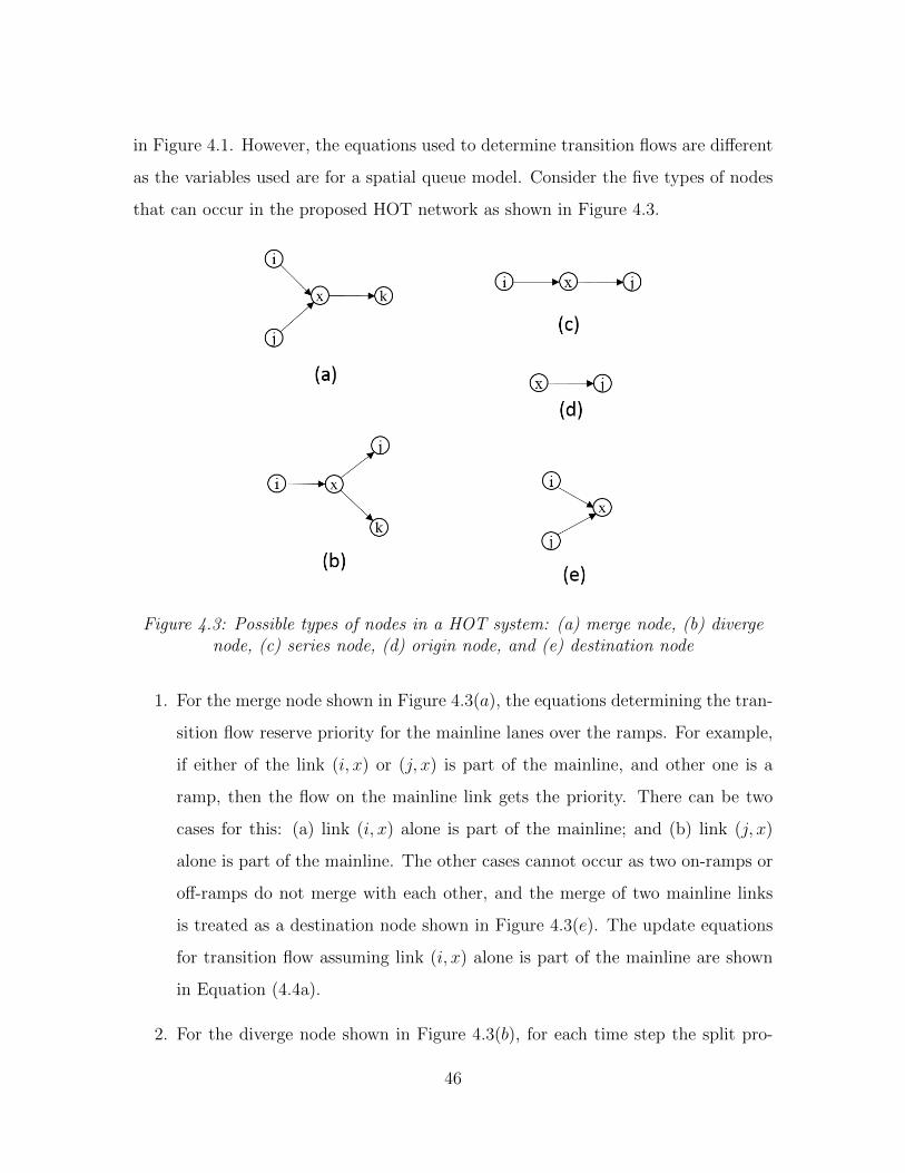
in Figure 4.1. However, the equations used to determine transition flows are different

as the variables used are for a spatial queue model. Consider the five types of nodes

that can occur in the proposed HOT network as shown in Figure 4.3.

Figure 4.3: Possible types of nodes in a HOT system: (a) merge node, (b) divergenode, (c) series node, (d) origin node, and (e) destination node

1. For the merge node shown in Figure 4.3(a), the equations determining the tran-

sition flow reserve priority for the mainline lanes over the ramps. For example,

if either of the link (i, x) or (j, x) is part of the mainline, and other one is a

ramp, then the flow on the mainline link gets the priority. There can be two

cases for this: (a) link (i, x) alone is part of the mainline; and (b) link (j, x)

alone is part of the mainline. The other cases cannot occur as two on-ramps or

off-ramps do not merge with each other, and the merge of two mainline links

is treated as a destination node shown in Figure 4.3(e). The update equations

for transition flow assuming link (i, x) alone is part of the mainline are shown

in Equation (4.4a).

2. For the diverge node shown in Figure 4.3(b), for each time step the split pro-

46

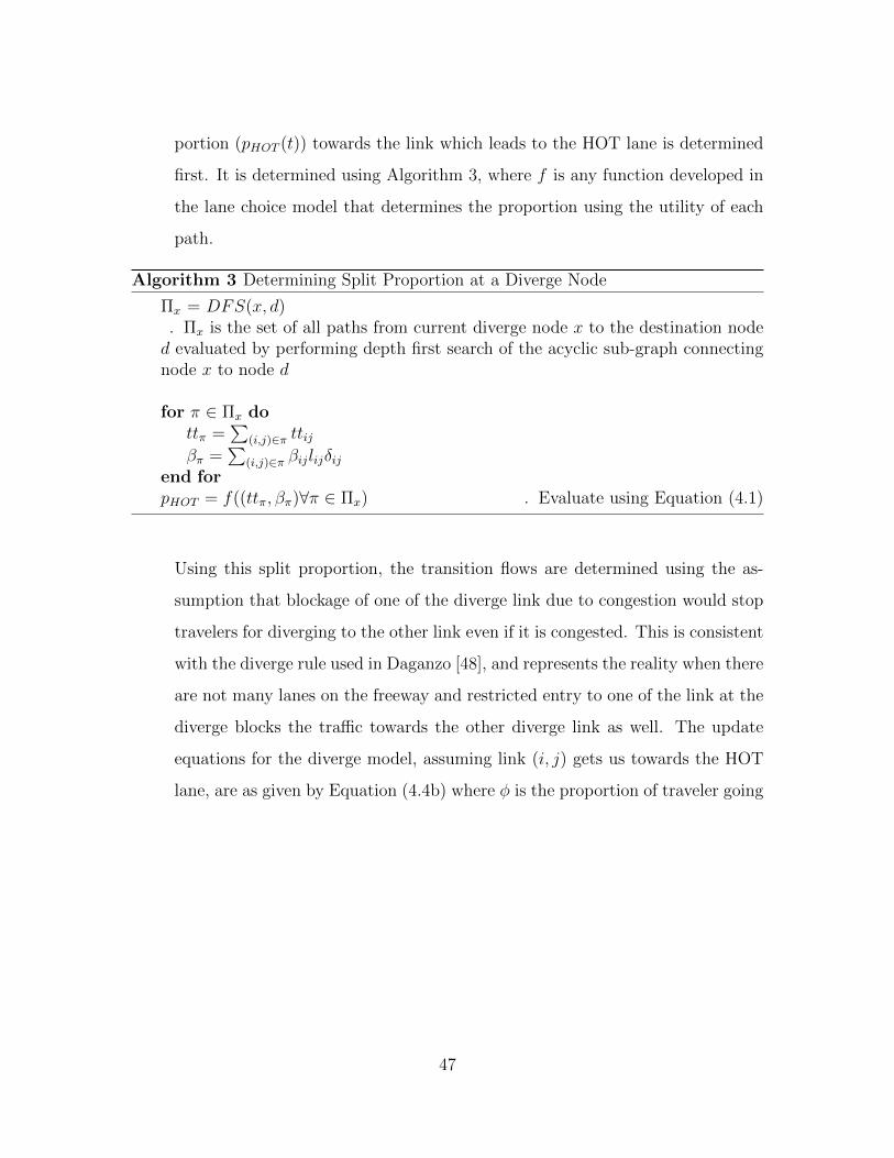
portion (pHOT (t)) towards the link which leads to the HOT lane is determined

first. It is determined using Algorithm 3, where f is any function developed in

the lane choice model that determines the proportion using the utility of each

path.

Algorithm 3 Determining Split Proportion at a Diverge Node

Πx = DFS(x, d). Πx is the set of all paths from current diverge node x to the destination noded evaluated by performing depth first search of the acyclic sub-graph connectingnode x to node d

for π ∈ Πx dottπ =

∑(i,j)∈π ttij

βπ =∑

(i,j)∈π βijlijδijend forpHOT = f((ttπ, βπ)∀π ∈ Πx) . Evaluate using Equation (4.1)

Using this split proportion, the transition flows are determined using the as-

sumption that blockage of one of the diverge link due to congestion would stop

travelers for diverging to the other link even if it is congested. This is consistent

with the diverge rule used in Daganzo [48], and represents the reality when there

are not many lanes on the freeway and restricted entry to one of the link at the

diverge blocks the traffic towards the other diverge link as well. The update

equations for the diverge model, assuming link (i, j) gets us towards the HOT

lane, are as given by Equation (4.4b) where φ is the proportion of traveler going

47

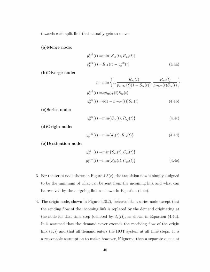
towards each split link that actually gets to move.

(a)Merge node:

yixkx (t) =min{Six(t), Rxk(t)}

yjxkx (t) =Rxk(t)− yixkx (t) (4.4a)

(b)Diverge node:

φ =min

{1,

Rxj(t)

pHOT (t)(1− Six(t)),

Rxk(t)

pHOT (t)Six(t)

}yixkx (t) =φpHOT (t)Six(t)

yixjx (t) =φ(1− pHOT (t))Six(t) (4.4b)

(c)Series node:

yixjx (t) =min{Six(t), Rxj(t)} (4.4c)

(d)Origin node:

y−xix (t) =min{dx(t), Rxi(t)} (4.4d)

(e)Destination node:

yix−x (t) =min{Six(t), Cix(t)}

yjx−x (t) =min{Sjx(t), Cjx(t)} (4.4e)

3. For the series node shown in Figure 4.3(c), the transition flow is simply assigned

to be the minimum of what can be sent from the incoming link and what can

be received by the outgoing link as shown in Equation (4.4c).

4. The origin node, shown in Figure 4.3(d), behaves like a series node except that

the sending flow of the incoming link is replaced by the demand originating at

the node for that time step (denoted by dx(t)), as shown in Equation (4.4d).

It is assumed that the demand never exceeds the receiving flow of the origin

link (x, i) and that all demand enters the HOT system at all time steps. It is

a reasonable assumption to make; however, if ignored then a separate queue at

48

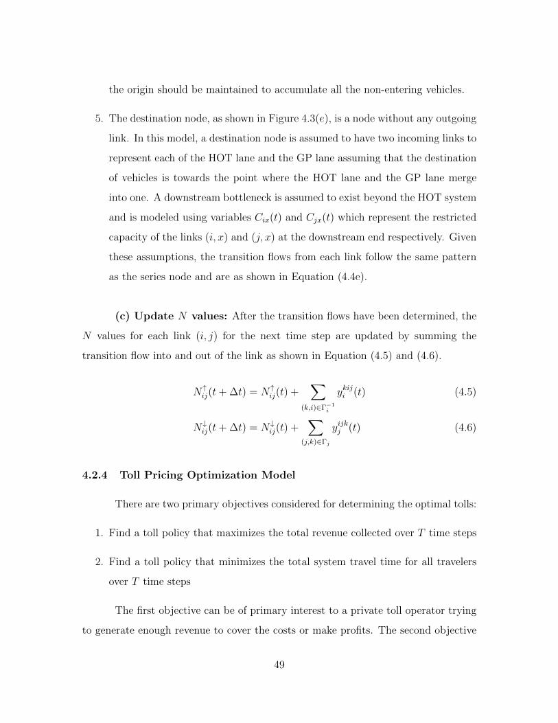
the origin should be maintained to accumulate all the non-entering vehicles.

5. The destination node, as shown in Figure 4.3(e), is a node without any outgoing

link. In this model, a destination node is assumed to have two incoming links to

represent each of the HOT lane and the GP lane assuming that the destination

of vehicles is towards the point where the HOT lane and the GP lane merge

into one. A downstream bottleneck is assumed to exist beyond the HOT system

and is modeled using variables Cix(t) and Cjx(t) which represent the restricted

capacity of the links (i, x) and (j, x) at the downstream end respectively. Given

these assumptions, the transition flows from each link follow the same pattern

as the series node and are as shown in Equation (4.4e).

(c) Update N values: After the transition flows have been determined, the

N values for each link (i, j) for the next time step are updated by summing the

transition flow into and out of the link as shown in Equation (4.5) and (4.6).

N↑ij(t+ ∆t) = N↑ij(t) +∑

(k,i)∈Γ−1i

ykiji (t) (4.5)

N↓ij(t+ ∆t) = N↓ij(t) +∑

(j,k)∈Γj

yijkj (t) (4.6)

4.2.4 Toll Pricing Optimization Model

There are two primary objectives considered for determining the optimal tolls:

1. Find a toll policy that maximizes the total revenue collected over T time steps

2. Find a toll policy that minimizes the total system travel time for all travelers

over T time steps

The first objective can be of primary interest to a private toll operator trying

to generate enough revenue to cover the costs or make profits. The second objective

49

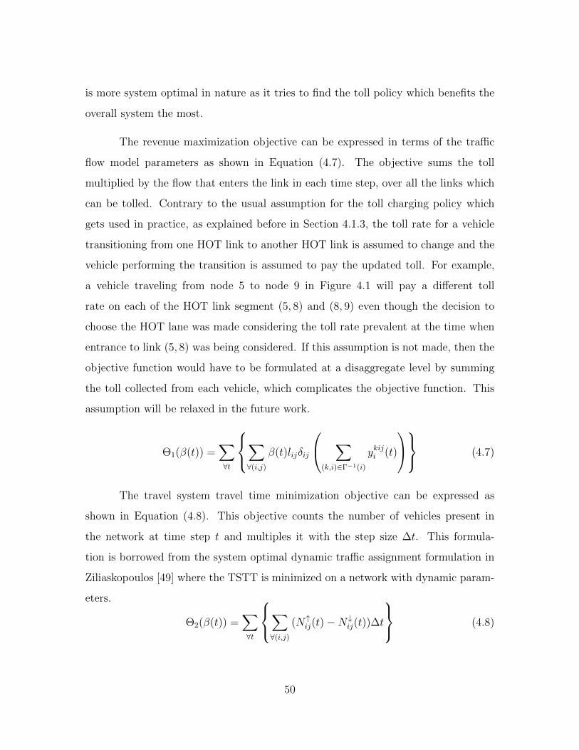
is more system optimal in nature as it tries to find the toll policy which benefits the

overall system the most.

The revenue maximization objective can be expressed in terms of the traffic

flow model parameters as shown in Equation (4.7). The objective sums the toll

multiplied by the flow that enters the link in each time step, over all the links which

can be tolled. Contrary to the usual assumption for the toll charging policy which

gets used in practice, as explained before in Section 4.1.3, the toll rate for a vehicle

transitioning from one HOT link to another HOT link is assumed to change and the

vehicle performing the transition is assumed to pay the updated toll. For example,

a vehicle traveling from node 5 to node 9 in Figure 4.1 will pay a different toll

rate on each of the HOT link segment (5, 8) and (8, 9) even though the decision to

choose the HOT lane was made considering the toll rate prevalent at the time when

entrance to link (5, 8) was being considered. If this assumption is not made, then the

objective function would have to be formulated at a disaggregate level by summing

the toll collected from each vehicle, which complicates the objective function. This

assumption will be relaxed in the future work.

Θ1(β(t)) =∑∀t

∑∀(i,j)

β(t)lijδij

∑(k,i)∈Γ−1(i)

ykiji (t)

(4.7)

The travel system travel time minimization objective can be expressed as

shown in Equation (4.8). This objective counts the number of vehicles present in

the network at time step t and multiples it with the step size ∆t. This formula-

tion is borrowed from the system optimal dynamic traffic assignment formulation in

Ziliaskopoulos [49] where the TSTT is minimized on a network with dynamic param-

eters.

Θ2(β(t)) =∑∀t

∑∀(i,j)

(N↑ij(t)−N↓ij(t))∆t

(4.8)

50

Given these objectives, the goal of the optimization problem is to find the

policy that achieves the proposed objective subject to the following constraints:

1. The traffic flows according to the proposed traffic flow model.

2. The travel time on the HOT lane is below a threshold (or is always equal to the

free-flow travel time).

3. The toll changes within a particular set (i.e. can not exceed a maximum or a

minimum value).

Constraint (1) models the propagation of the traffic and updates the link and

node parameters with time. Constraint (2) represents the restriction that the HOT

lane must always provide a minimum speed limit, and that travel time on the lane

can not drop below a particular value (usually assumed to be the free-flow travel

time). Constraint (3) captures the toll related regulations where tolls can not exceed

beyond a particular limit, and are usually set above a minimum limit. Additional

constraint which controls the rate of change of the toll are also relevant in practice;

however, considering the complication of the framed optimization problem they are

not included as part of this study.

Combining all of this the optimization problem can be represented as in Equa-

tion (4.9).

max/minβ(t)

Θi i ∈ {1, 2} (4.9a)

subject to

Equations (4.2)− (4.6) (4.9b)

τij(t) ≤ T thresholdij ∀(i, j) ∈ AHOT (4.9c)

β(t) ∈ (βmin, βmax) (4.9d)

51

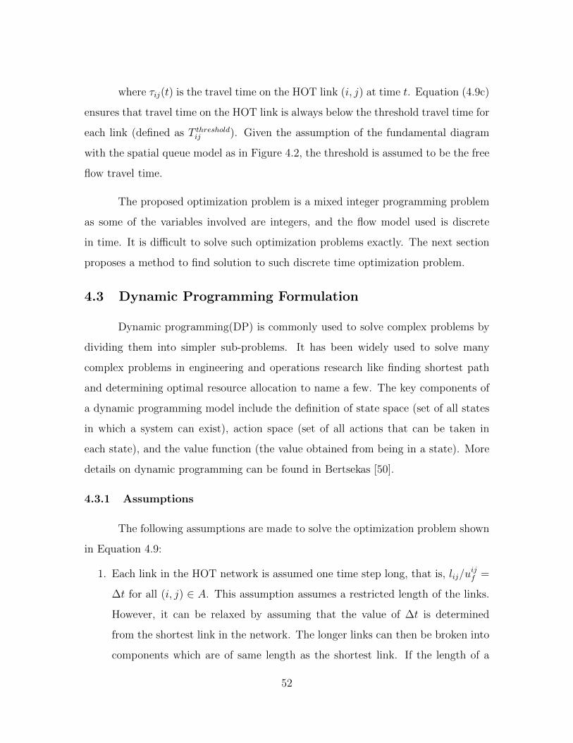
where τij(t) is the travel time on the HOT link (i, j) at time t. Equation (4.9c)

ensures that travel time on the HOT link is always below the threshold travel time for

each link (defined as T thresholdij ). Given the assumption of the fundamental diagram

with the spatial queue model as in Figure 4.2, the threshold is assumed to be the free

flow travel time.

The proposed optimization problem is a mixed integer programming problem

as some of the variables involved are integers, and the flow model used is discrete

in time. It is difficult to solve such optimization problems exactly. The next section

proposes a method to find solution to such discrete time optimization problem.

4.3 Dynamic Programming Formulation

Dynamic programming(DP) is commonly used to solve complex problems by

dividing them into simpler sub-problems. It has been widely used to solve many

complex problems in engineering and operations research like finding shortest path

and determining optimal resource allocation to name a few. The key components of

a dynamic programming model include the definition of state space (set of all states

in which a system can exist), action space (set of all actions that can be taken in

each state), and the value function (the value obtained from being in a state). More

details on dynamic programming can be found in Bertsekas [50].

4.3.1 Assumptions

The following assumptions are made to solve the optimization problem shown

in Equation 4.9:

1. Each link in the HOT network is assumed one time step long, that is, lij/uijf =

∆t for all (i, j) ∈ A. This assumption assumes a restricted length of the links.

However, it can be relaxed by assuming that the value of ∆t is determined

from the shortest link in the network. The longer links can then be broken into

components which are of same length as the shortest link. If the length of a

52

longer link cannot be written as an integer multiple of the length of the shortest

link, rounding approximations can be made.

2. The spatial queue model is used (as described in the previous section) and the

fundamental diagram for the links is assumed to be same as Figure 4.2. The

instantaneous travel time on each link (i, j) is calculated as the sum of the

average time it takes to dissipate the queue and the time to traverse the link

(which is assumed to be one time step long), as shown in (4.10). It is assumed

that on an average the exit flow out of a link is half the exit capacity. Other

definitions of instantaneous travel time will be considered as part of the future

work.

ttij(t) = ∆t+vqij(t)

qijmax/2(4.10)

3. The toll set is assumed to be discrete and finite, and thus the tolls can only

be varied within the toll set. This discretization is needed to ensure that the

dynamic programming algorithm remains computationally tractable.

4. It is assumed that the demand entering the network does not exceed the capacity

of the link coming out of the origin, and all vehicles get to enter the network

at all time steps. This assumption is reasonable if there is no queue spillback

from the downstream links leading up to the origin.

5. It is assumed that the vehicles are discrete and atomic, and the flow values are

always an integer. In order to achieve this, the flow values are rounded to the

nearest integer at each time step.

4.3.2 State Space, Action Space, and Value Function

State Space: In order to define the state space for the dynamic programming

formulation, the following vehicle variables are introduced for each link (i, j):

• vlij(t): Number of vehicles traveling on link (i, j) at time t

53

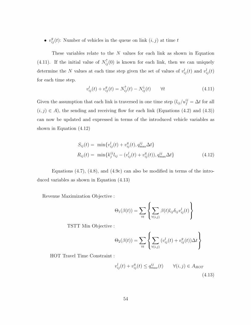
• vqij(t): Number of vehicles in the queue on link (i, j) at time t

These variables relate to the N values for each link as shown in Equation

(4.11). If the initial value of N↑ij(0) is known for each link, then we can uniquely

determine the N values at each time step given the set of values of vlij(t) and vlij(t)

for each time step.

vlij(t) + vqij(t) = N↑ij(t)−N↓ij(t) ∀t (4.11)

Given the assumption that each link is traversed in one time step (lij/uijf = ∆t for all

(i, j) ∈ A), the sending and receiving flow for each link (Equations (4.2) and (4.3))

can now be updated and expressed in terms of the introduced vehicle variables as

shown in Equation (4.12)

Sij(t) = min{vlij(t) + vqij(t), qijmax∆t}

Rij(t) = min{kijj lij − (vlij(t) + vqij(t)), qijmax∆t} (4.12)

Equations (4.7), (4.8), and (4.9c) can also be modified in terms of the intro-

duced variables as shown in Equation (4.13)

Revenue Maximization Objective :

Θ1(β(t)) =∑∀t

∑∀(i,j)

β(t)lijδijvlij(t)

TSTT Min Objective :

Θ2(β(t)) =∑∀t

∑∀(i,j)

(vlij(t) + vqij(t))∆t

HOT Travel Time Constraint :

vlij(t) + vqij(t) ≤ qijmax(t) ∀(i, j) ∈ AHOT(4.13)

54

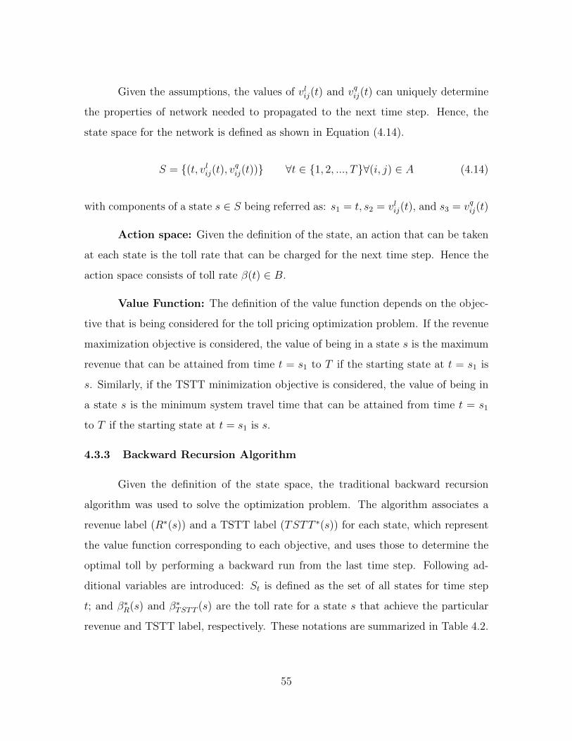
Given the assumptions, the values of vlij(t) and vqij(t) can uniquely determine

the properties of network needed to propagated to the next time step. Hence, the

state space for the network is defined as shown in Equation (4.14).

S = {(t, vlij(t), vqij(t))} ∀t ∈ {1, 2, ..., T}∀(i, j) ∈ A (4.14)

with components of a state s ∈ S being referred as: s1 = t, s2 = vlij(t), and s3 = vqij(t)

Action space: Given the definition of the state, an action that can be taken

at each state is the toll rate that can be charged for the next time step. Hence the

action space consists of toll rate β(t) ∈ B.

Value Function: The definition of the value function depends on the objec-

tive that is being considered for the toll pricing optimization problem. If the revenue

maximization objective is considered, the value of being in a state s is the maximum

revenue that can be attained from time t = s1 to T if the starting state at t = s1 is

s. Similarly, if the TSTT minimization objective is considered, the value of being in

a state s is the minimum system travel time that can be attained from time t = s1

to T if the starting state at t = s1 is s.

4.3.3 Backward Recursion Algorithm

Given the definition of the state space, the traditional backward recursion

algorithm was used to solve the optimization problem. The algorithm associates a

revenue label (R∗(s)) and a TSTT label (TSTT ∗(s)) for each state, which represent

the value function corresponding to each objective, and uses those to determine the

optimal toll by performing a backward run from the last time step. Following ad-

ditional variables are introduced: St is defined as the set of all states for time step

t; and β∗R(s) and β∗TSTT (s) are the toll rate for a state s that achieve the particular

revenue and TSTT label, respectively. These notations are summarized in Table 4.2.

55

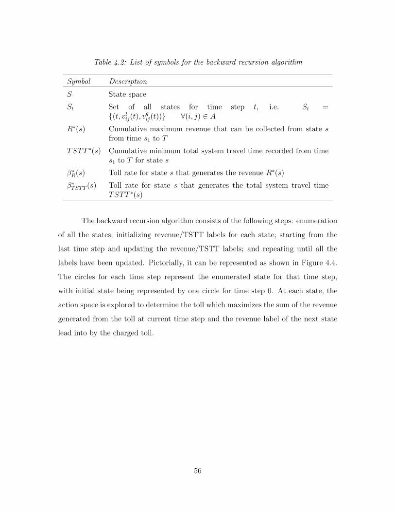
Table 4.2: List of symbols for the backward recursion algorithm

Symbol Description

S State space

St Set of all states for time step t, i.e. St ={(t, vlij(t), v

qij(t))} ∀(i, j) ∈ A

R∗(s) Cumulative maximum revenue that can be collected from state sfrom time s1 to T

TSTT ∗(s) Cumulative minimum total system travel time recorded from times1 to T for state s

β∗R(s) Toll rate for state s that generates the revenue R∗(s)

β∗TSTT (s) Toll rate for state s that generates the total system travel timeTSTT ∗(s)

The backward recursion algorithm consists of the following steps: enumeration

of all the states; initializing revenue/TSTT labels for each state; starting from the

last time step and updating the revenue/TSTT labels; and repeating until all the

labels have been updated. Pictorially, it can be represented as shown in Figure 4.4.

The circles for each time step represent the enumerated state for that time step,

with initial state being represented by one circle for time step 0. At each state, the

action space is explored to determine the toll which maximizes the sum of the revenue

generated from the toll at current time step and the revenue label of the next state

lead into by the charged toll.

56

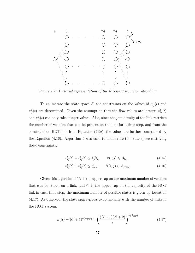
Figure 4.4: Pictorial representation of the backward recursion algorithm

To enumerate the state space S, the constraints on the values of vlij(t) and

vqij(t) are determined. Given the assumption that the flow values are integer, vlij(t)

and vqij(t) can only take integer values. Also, since the jam density of the link restricts

the number of vehicles that can be present on the link for a time step, and from the

constraint on HOT link from Equation (4.9c), the values are further constrained by

the Equation (4.16). Algorithm 4 was used to enumerate the state space satisfying

these constraints.

vlij(t) + vqij(t) ≤ kijj lij ∀(i, j) ∈ AGP (4.15)

vlij(t) + vqij(t) ≤ qijmax ∀(i, j) ∈ AHOT (4.16)

Given this algorithm, if N is the upper cap on the maximum number of vehicles

that can be stored on a link, and C is the upper cap on the capacity of the HOT

link in each time step, the maximum number of possible states is given by Equation

(4.17). As observed, the state space grows exponentially with the number of links in

the HOT system.

n(S) = (C + 1)n(AHOT ) ·(

(N + 1)(N + 2)

2

)n(AGP )

(4.17)

57

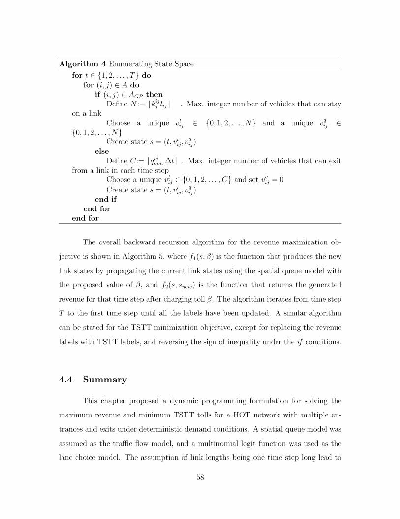
Algorithm 4 Enumerating State Space

for t ∈ {1, 2, . . . , T} dofor (i, j) ∈ A do

if (i, j) ∈ AGP thenDefine N := bkijj lijc . Max. integer number of vehicles that can stay

on a linkChoose a unique vlij ∈ {0, 1, 2, . . . , N} and a unique vqij ∈

{0, 1, 2, . . . , N}Create state s = (t, vlij, v

qij)

elseDefine C:= bqijmax∆tc . Max. integer number of vehicles that can exit

from a link in each time stepChoose a unique vlij ∈ {0, 1, 2, . . . , C} and set vqij = 0

Create state s = (t, vlij, vqij)

end ifend for

end for

The overall backward recursion algorithm for the revenue maximization ob-

jective is shown in Algorithm 5, where f1(s, β) is the function that produces the new

link states by propagating the current link states using the spatial queue model with

the proposed value of β, and f2(s, snew) is the function that returns the generated

revenue for that time step after charging toll β. The algorithm iterates from time step

T to the first time step until all the labels have been updated. A similar algorithm

can be stated for the TSTT minimization objective, except for replacing the revenue

labels with TSTT labels, and reversing the sign of inequality under the if conditions.

4.4 Summary

This chapter proposed a dynamic programming formulation for solving the

maximum revenue and minimum TSTT tolls for a HOT network with multiple en-

trances and exits under deterministic demand conditions. A spatial queue model was

assumed as the traffic flow model, and a multinomial logit function was used as the

lane choice model. The assumption of link lengths being one time step long lead to

58

Algorithm 5 Backward Recursion Algorithm

Step 0: Enumerate and initialize label for all statesR∗(s) := 0∀s ∈ S

Step 1: Update revenue labels for last time stepfor s ∈ ST do

maxRev = −1for β ∈ B do

snew = f1(s, β)Rev = f2(s, snew)if Rev > maxRev then

maxRev = Revβ∗R(s) = βR∗(s) = maxRev

end ifend for

end for

Step 2: Update revenue labels for all previous time stepfor t ∈ {0, 1, 2, . . . , T − 1} in reverse order do

for s ∈ St domaxRev = −1for β ∈ B do

snew = f1(s, β)Rev = f2(s, snew) +R∗(snew)if Rev > maxRev then

maxRev = Revβ∗R(s) = βR∗(s) = maxRev

end ifend for

end forend for

59

an easier definition of the state space consisting only of the vehicles currently travel-

ing on the link and the vehicles present in the spatial queue. A backward recursion

algorithm was proposed to solve for optimal tolls starting from the last time step and

updating the value function labels until all enumerated states are assigned a label.

Such an algorithm can solve for the optimal tolls exactly [50]. The demonstration of

the algorithm on different test networks is presented in the next chapter.

60

Chapter 5

Results

This chapter presents the results from the analysis performed using the method

defined in the Chapter 4. The focus is on testing the performance of the backward

recursion algorithm for a simple network for a limited number of time steps to offer

a better understanding of the results. Additional experiments are then conducted

to compare the optimal tolls for two different lane choice models, to compare the

performance of the backward recursion algorithm on slightly larger networks, and to

quantify the performance of the myopic policies for revenue maximization.

5.1 Application of the Dynamic Programming Algorithm

The dynamic programming algorithm proposed in the previous chapter was

coded in Java, and was tested on a small network to demonstrate the application

and optimality of the proposed algorithm. A single entrance single exit network, as

shown in Figure 5.1, was chosen for the analysis. The top path between nodes 2 and

3 represents an HOT lane while the bottom path represents the parallel GP lane.

Two simulations were performed on the proposed network:

1. Simulation 1 was run for a restricted toll set, β(t) ∈ {0.2, 0.3, 0.4, 0.5, 0.6}, for

four time steps. The results of the simulation were compared with the results of

all possible toll policies, enumerated to demonstrate the optimality of the DP

algorithm

2. Simulation 2 was run for 20 time steps over a broader set of tolls

61

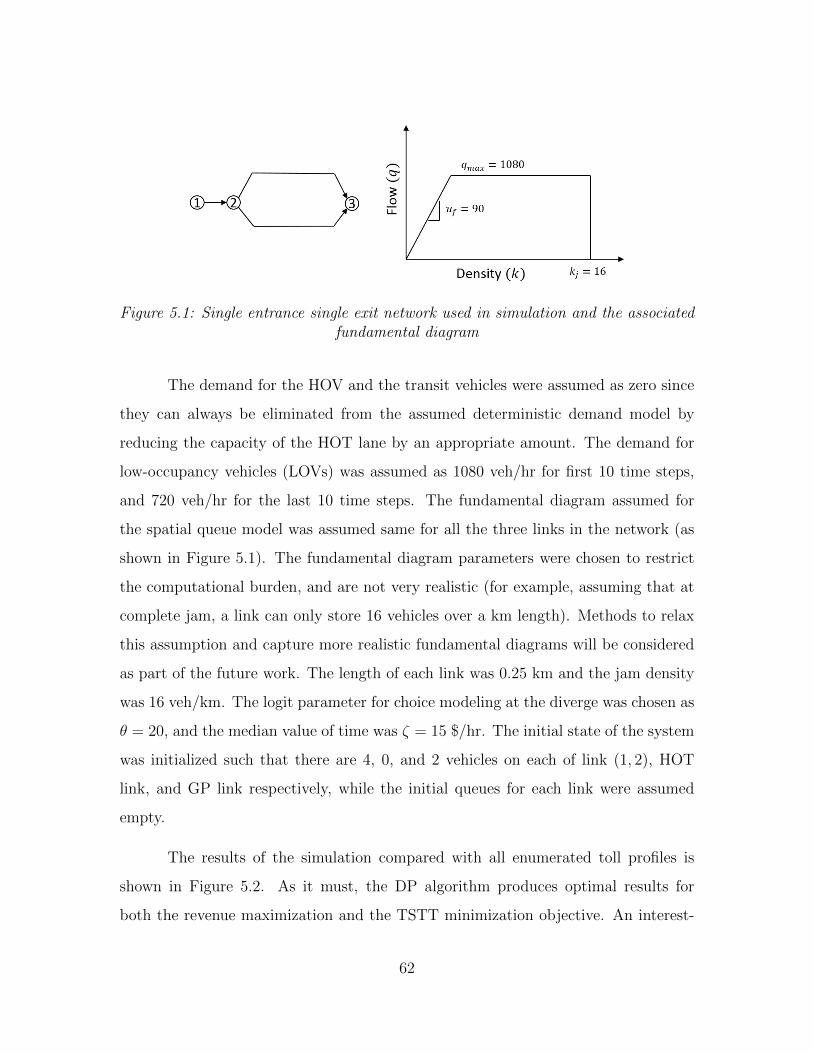
Figure 5.1: Single entrance single exit network used in simulation and the associatedfundamental diagram

The demand for the HOV and the transit vehicles were assumed as zero since

they can always be eliminated from the assumed deterministic demand model by

reducing the capacity of the HOT lane by an appropriate amount. The demand for

low-occupancy vehicles (LOVs) was assumed as 1080 veh/hr for first 10 time steps,

and 720 veh/hr for the last 10 time steps. The fundamental diagram assumed for

the spatial queue model was assumed same for all the three links in the network (as

shown in Figure 5.1). The fundamental diagram parameters were chosen to restrict

the computational burden, and are not very realistic (for example, assuming that at

complete jam, a link can only store 16 vehicles over a km length). Methods to relax

this assumption and capture more realistic fundamental diagrams will be considered

as part of the future work. The length of each link was 0.25 km and the jam density

was 16 veh/km. The logit parameter for choice modeling at the diverge was chosen as

θ = 20, and the median value of time was ζ = 15 $/hr. The initial state of the system

was initialized such that there are 4, 0, and 2 vehicles on each of link (1, 2), HOT

link, and GP link respectively, while the initial queues for each link were assumed

empty.

The results of the simulation compared with all enumerated toll profiles is

shown in Figure 5.2. As it must, the DP algorithm produces optimal results for

both the revenue maximization and the TSTT minimization objective. An interest-

62

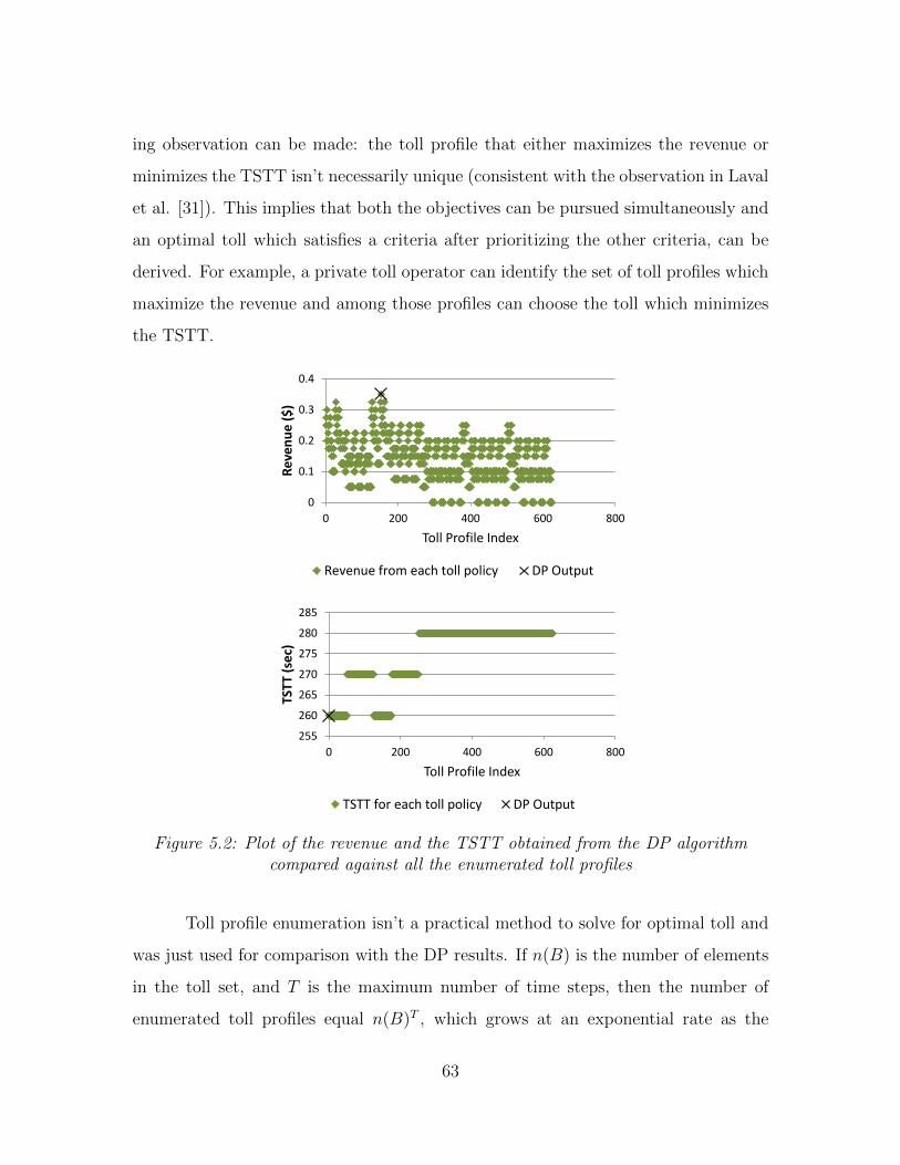
ing observation can be made: the toll profile that either maximizes the revenue or

minimizes the TSTT isn’t necessarily unique (consistent with the observation in Laval

et al. [31]). This implies that both the objectives can be pursued simultaneously and

an optimal toll which satisfies a criteria after prioritizing the other criteria, can be

derived. For example, a private toll operator can identify the set of toll profiles which

maximize the revenue and among those profiles can choose the toll which minimizes

the TSTT.

0

0.1

0.2

0.3

0.4

0 200 400 600 800

Rev

en

ue

($

)

Toll Profile Index

Revenue from each toll policy DP Output

255

260

265

270

275

280

285

0 200 400 600 800

TST

T (s

ec)

Toll Profile Index

TSTT for each toll policy DP Output

Figure 5.2: Plot of the revenue and the TSTT obtained from the DP algorithmcompared against all the enumerated toll profiles

Toll profile enumeration isn’t a practical method to solve for optimal toll and

was just used for comparison with the DP results. If n(B) is the number of elements

in the toll set, and T is the maximum number of time steps, then the number of

enumerated toll profiles equal n(B)T , which grows at an exponential rate as the

63

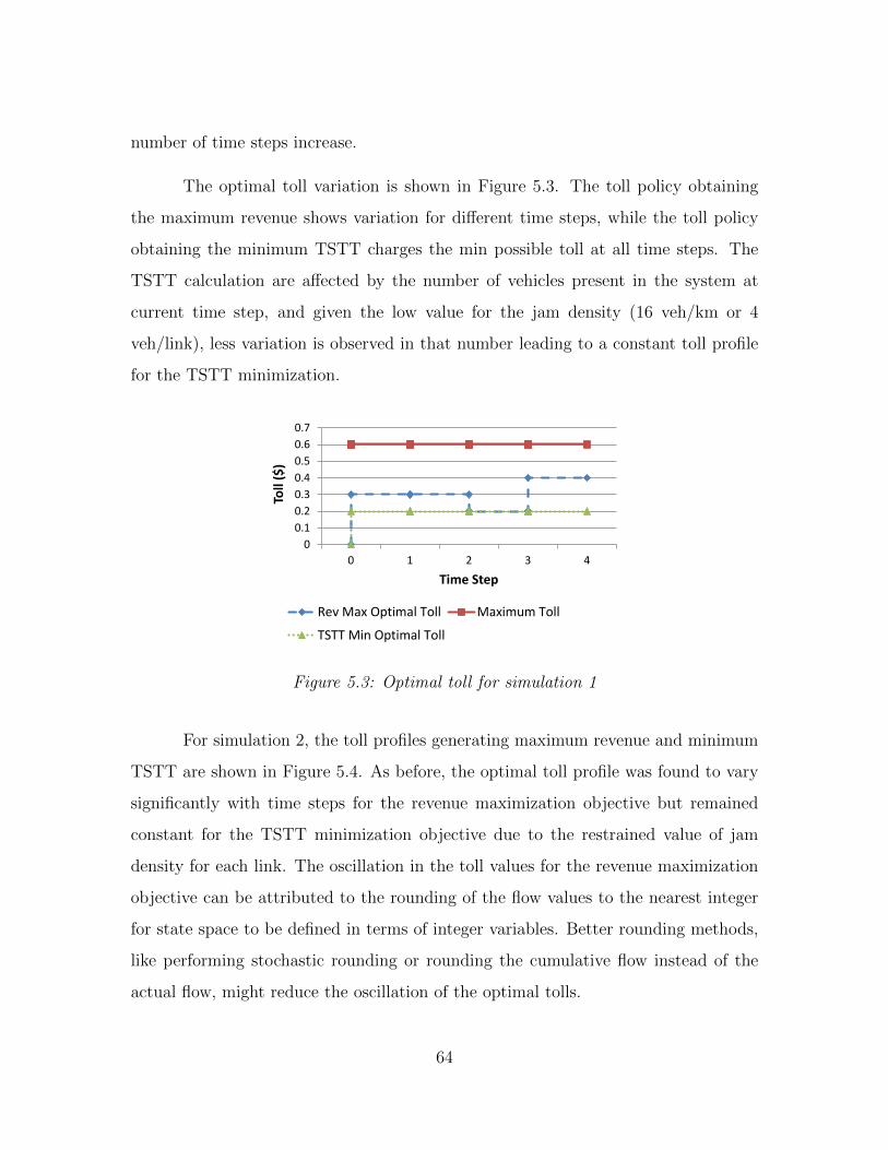
number of time steps increase.

The optimal toll variation is shown in Figure 5.3. The toll policy obtaining

the maximum revenue shows variation for different time steps, while the toll policy

obtaining the minimum TSTT charges the min possible toll at all time steps. The

TSTT calculation are affected by the number of vehicles present in the system at

current time step, and given the low value for the jam density (16 veh/km or 4

veh/link), less variation is observed in that number leading to a constant toll profile

for the TSTT minimization.

0

0.1

0.2

0.3

0.4

0.5

0.6

0.7

0 1 2 3 4

Toll

($)

Time Step

Rev Max Optimal Toll Maximum Toll

TSTT Min Optimal Toll

Figure 5.3: Optimal toll for simulation 1

For simulation 2, the toll profiles generating maximum revenue and minimum

TSTT are shown in Figure 5.4. As before, the optimal toll profile was found to vary

significantly with time steps for the revenue maximization objective but remained

constant for the TSTT minimization objective due to the restrained value of jam

density for each link. The oscillation in the toll values for the revenue maximization

objective can be attributed to the rounding of the flow values to the nearest integer

for state space to be defined in terms of integer variables. Better rounding methods,

like performing stochastic rounding or rounding the cumulative flow instead of the

actual flow, might reduce the oscillation of the optimal tolls.

64

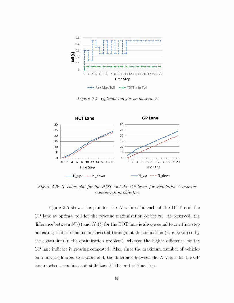
0

0.1

0.2

0.3

0.4

0.5

0 1 2 3 4 5 6 7 8 9 10 11 12 13 14 15 16 17 18 19 20To

ll ($

)

Time Step

Rev Max Toll TSTT min Toll

Figure 5.4: Optimal toll for simulation 2

0

5

10

15

20

25

30

0 2 4 6 8 10 12 14 16 18 20

Time Step

HOT Lane

N_up N_down

0

5

10

15

20

25

30

0 2 4 6 8 10 12 14 16 18 20

Time Step

GP Lane

N_up N_down

Figure 5.5: N value plot for the HOT and the GP lanes for simulation 2 revenuemaximization objective

Figure 5.5 shows the plot for the N values for each of the HOT and the

GP lane at optimal toll for the revenue maximization objective. As observed, the

difference between N↑(t) and N↓(t) for the HOT lane is always equal to one time step

indicating that it remains uncongested throughout the simulation (as guaranteed by

the constraints in the optimization problem), whereas the higher difference for the

GP lane indicate it growing congested. Also, since the maximum number of vehicles

on a link are limited to a value of 4, the difference between the N values for the GP

lane reaches a maxima and stabilizes till the end of time step.

65

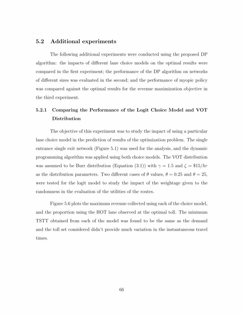
5.2 Additional experiments

The following additional experiments were conducted using the proposed DP

algorithm: the impacts of different lane choice models on the optimal results were

compared in the first experiment; the performance of the DP algorithm on networks

of different sizes was evaluated in the second; and the performance of myopic policy

was compared against the optimal results for the revenue maximization objective in

the third experiment.

5.2.1 Comparing the Performance of the Logit Choice Model and VOT

Distribution

The objective of this experiment was to study the impact of using a particular

lane choice model in the prediction of results of the optimization problem. The single

entrance single exit network (Figure 5.1) was used for the analysis, and the dynamic

programming algorithm was applied using both choice models. The VOT distribution

was assumed to be Burr distribution (Equation (3.1)) with γ = 1.5 and ζ = $15/hr

as the distribution parameters. Two different cases of θ values, θ = 0.25 and θ = 25,

were tested for the logit model to study the impact of the weightage given to the

randomness in the evaluation of the utilities of the routes.

Figure 5.6 plots the maximum revenue collected using each of the choice model,

and the proportion using the HOT lane observed at the optimal toll. The minimum

TSTT obtained from each of the model was found to be the same as the demand

and the toll set considered didn’t provide much variation in the instantaneous travel

times.

66

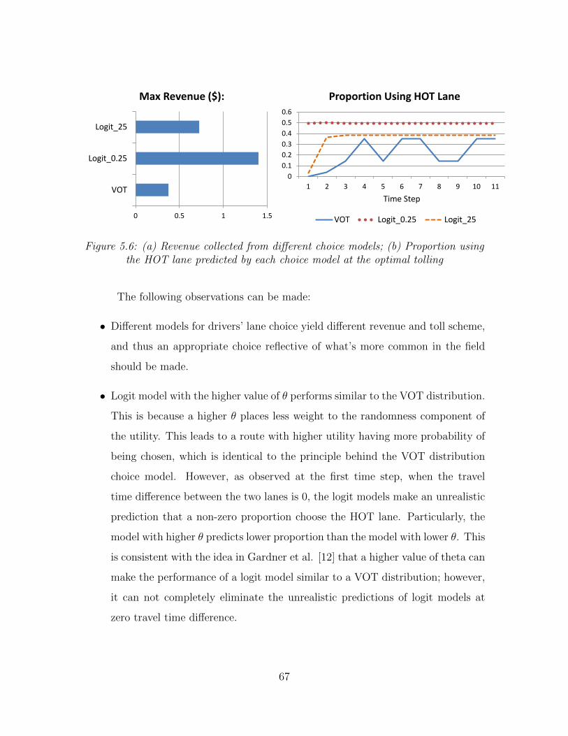
0 0.5 1 1.5

VOT

Logit_0.25

Logit_25

Max Revenue ($):

0

0.1

0.2

0.3

0.4

0.5

0.6

1 2 3 4 5 6 7 8 9 10 11

Time Step

Proportion Using HOT Lane

VOT Logit_0.25 Logit_25

Figure 5.6: (a) Revenue collected from different choice models; (b) Proportion usingthe HOT lane predicted by each choice model at the optimal tolling

The following observations can be made:

• Different models for drivers’ lane choice yield different revenue and toll scheme,

and thus an appropriate choice reflective of what’s more common in the field

should be made.

• Logit model with the higher value of θ performs similar to the VOT distribution.

This is because a higher θ places less weight to the randomness component of

the utility. This leads to a route with higher utility having more probability of

being chosen, which is identical to the principle behind the VOT distribution

choice model. However, as observed at the first time step, when the travel

time difference between the two lanes is 0, the logit models make an unrealistic

prediction that a non-zero proportion choose the HOT lane. Particularly, the

model with higher θ predicts lower proportion than the model with lower θ. This

is consistent with the idea in Gardner et al. [12] that a higher value of theta can

make the performance of a logit model similar to a VOT distribution; however,

it can not completely eliminate the unrealistic predictions of logit models at

zero travel time difference.

67

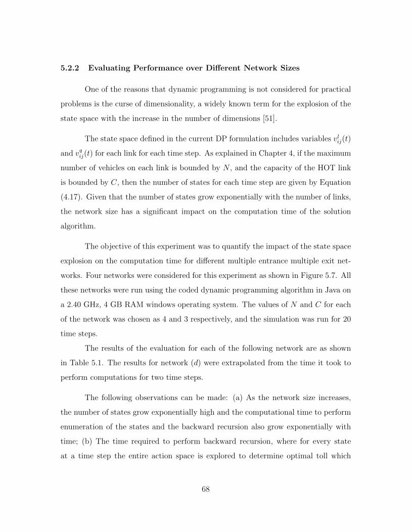
5.2.2 Evaluating Performance over Different Network Sizes

One of the reasons that dynamic programming is not considered for practical

problems is the curse of dimensionality, a widely known term for the explosion of the

state space with the increase in the number of dimensions [51].

The state space defined in the current DP formulation includes variables vlij(t)

and vqij(t) for each link for each time step. As explained in Chapter 4, if the maximum

number of vehicles on each link is bounded by N , and the capacity of the HOT link

is bounded by C, then the number of states for each time step are given by Equation

(4.17). Given that the number of states grow exponentially with the number of links,

the network size has a significant impact on the computation time of the solution

algorithm.

The objective of this experiment was to quantify the impact of the state space

explosion on the computation time for different multiple entrance multiple exit net-

works. Four networks were considered for this experiment as shown in Figure 5.7. All

these networks were run using the coded dynamic programming algorithm in Java on

a 2.40 GHz, 4 GB RAM windows operating system. The values of N and C for each

of the network was chosen as 4 and 3 respectively, and the simulation was run for 20

time steps.

The results of the evaluation for each of the following network are as shown

in Table 5.1. The results for network (d) were extrapolated from the time it took to

perform computations for two time steps.

The following observations can be made: (a) As the network size increases,

the number of states grow exponentially high and the computational time to perform

enumeration of the states and the backward recursion also grow exponentially with

time; (b) The time required to perform backward recursion, where for every state

at a time step the entire action space is explored to determine optimal toll which

68

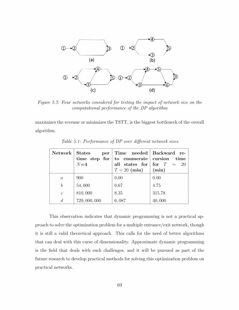
Figure 5.7: Four networks considered for testing the impact of network size on thecomputational performance of the DP algorithm

maximizes the revenue or minimizes the TSTT, is the biggest bottleneck of the overall

algorithm.

Table 5.1: Performance of DP over different network sizes

Network States pertime step forN=4

Time neededto enumerateall states forT = 20 (min)

Backward re-cursion timefor T = 20(min)

a 900 0.00 0.00

b 54, 000 0.67 4.75

c 810, 000 8.35 315.78

d 729, 000, 000 6, 087 40, 000

This observation indicates that dynamic programming is not a practical ap-

proach to solve the optimization problem for a multiple entrance/exit network, though

it is still a valid theoretical approach. This calls for the need of better algorithms

that can deal with this curse of dimensionality. Approximate dynamic programming

is the field that deals with such challenges, and it will be pursued as part of the

future research to develop practical methods for solving this optimization problem on

practical networks.

69

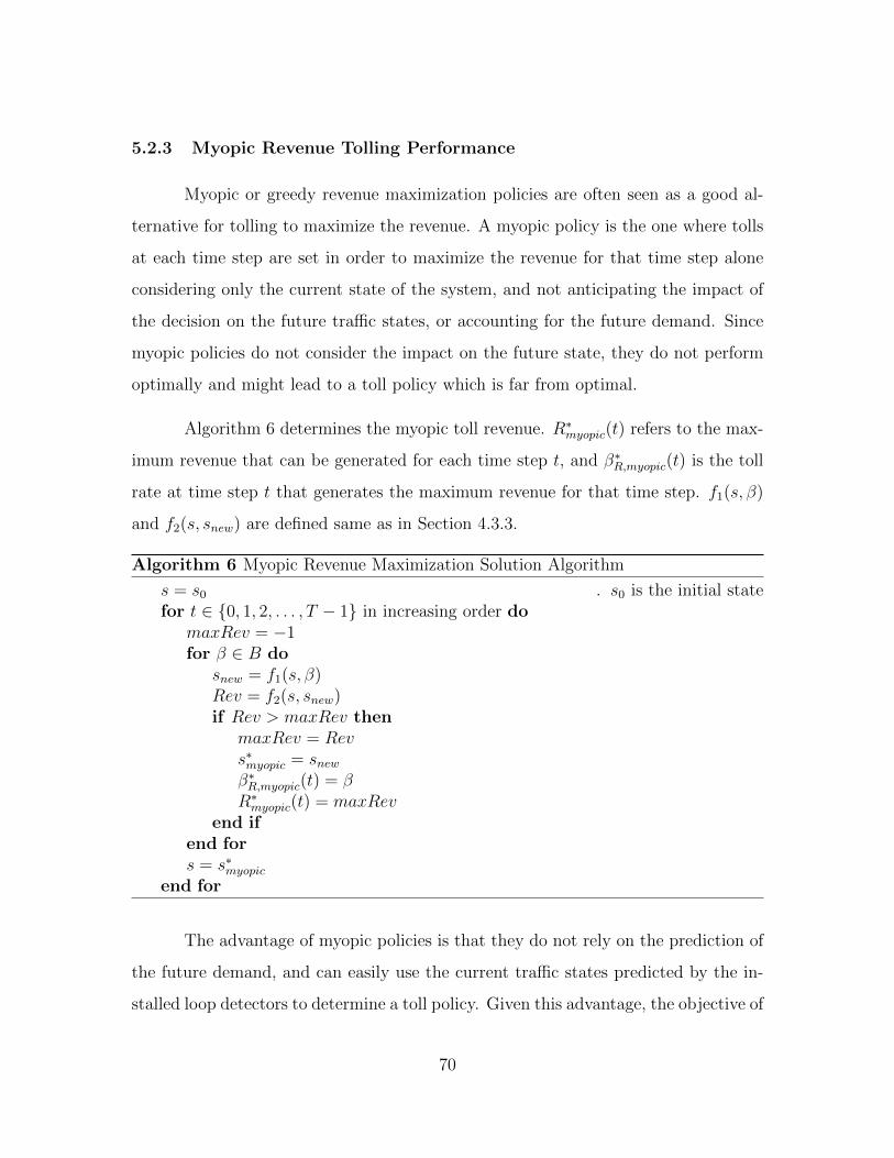
5.2.3 Myopic Revenue Tolling Performance

Myopic or greedy revenue maximization policies are often seen as a good al-

ternative for tolling to maximize the revenue. A myopic policy is the one where tolls

at each time step are set in order to maximize the revenue for that time step alone

considering only the current state of the system, and not anticipating the impact of

the decision on the future traffic states, or accounting for the future demand. Since

myopic policies do not consider the impact on the future state, they do not perform

optimally and might lead to a toll policy which is far from optimal.

Algorithm 6 determines the myopic toll revenue. R∗myopic(t) refers to the max-

imum revenue that can be generated for each time step t, and β∗R,myopic(t) is the toll

rate at time step t that generates the maximum revenue for that time step. f1(s, β)

and f2(s, snew) are defined same as in Section 4.3.3.

Algorithm 6 Myopic Revenue Maximization Solution Algorithm

s = s0 . s0 is the initial statefor t ∈ {0, 1, 2, . . . , T − 1} in increasing order do

maxRev = −1for β ∈ B do

snew = f1(s, β)Rev = f2(s, snew)if Rev > maxRev then

maxRev = Revs∗myopic = snewβ∗R,myopic(t) = βR∗myopic(t) = maxRev

end ifend fors = s∗myopic

end for

The advantage of myopic policies is that they do not rely on the prediction of

the future demand, and can easily use the current traffic states predicted by the in-

stalled loop detectors to determine a toll policy. Given this advantage, the objective of

70

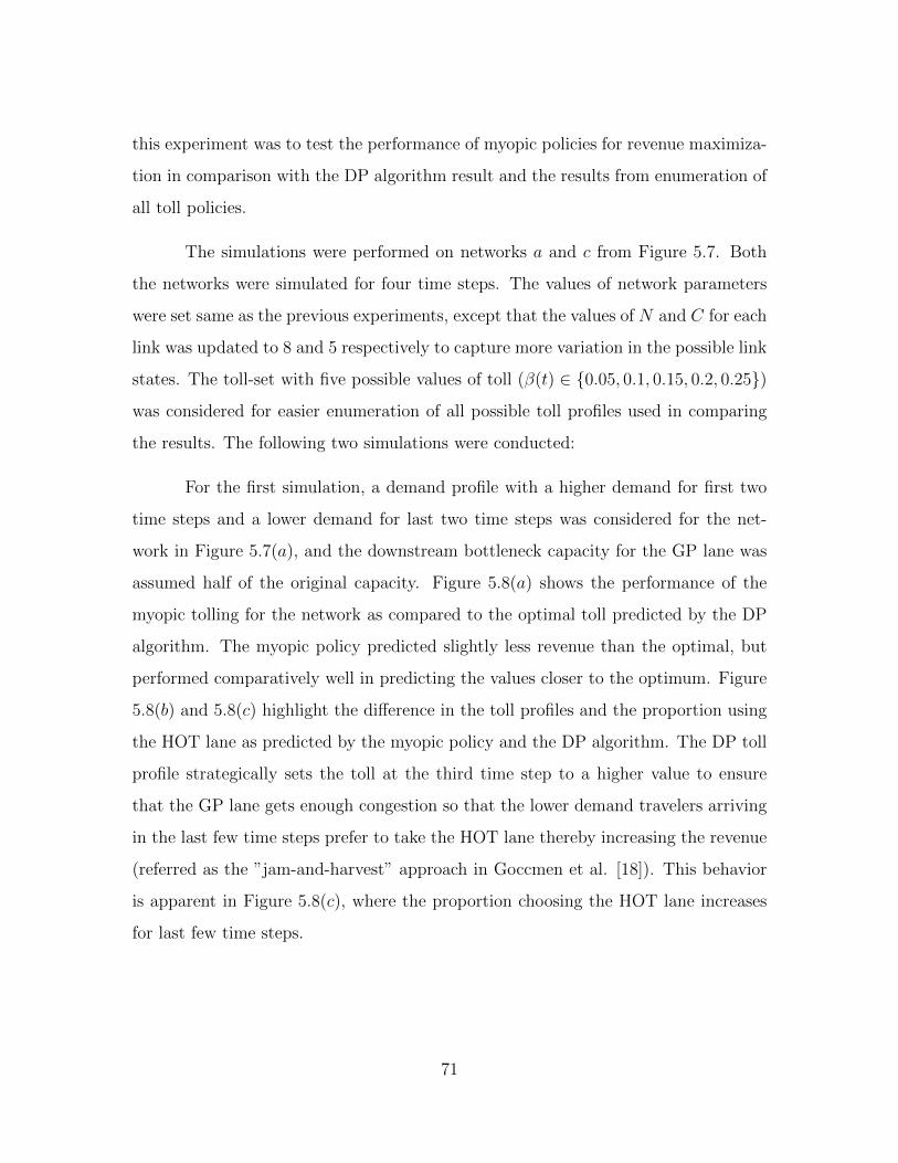
this experiment was to test the performance of myopic policies for revenue maximiza-

tion in comparison with the DP algorithm result and the results from enumeration of

all toll policies.

The simulations were performed on networks a and c from Figure 5.7. Both

the networks were simulated for four time steps. The values of network parameters

were set same as the previous experiments, except that the values of N and C for each

link was updated to 8 and 5 respectively to capture more variation in the possible link

states. The toll-set with five possible values of toll (β(t) ∈ {0.05, 0.1, 0.15, 0.2, 0.25})

was considered for easier enumeration of all possible toll profiles used in comparing

the results. The following two simulations were conducted:

For the first simulation, a demand profile with a higher demand for first two

time steps and a lower demand for last two time steps was considered for the net-

work in Figure 5.7(a), and the downstream bottleneck capacity for the GP lane was

assumed half of the original capacity. Figure 5.8(a) shows the performance of the

myopic tolling for the network as compared to the optimal toll predicted by the DP

algorithm. The myopic policy predicted slightly less revenue than the optimal, but

performed comparatively well in predicting the values closer to the optimum. Figure

5.8(b) and 5.8(c) highlight the difference in the toll profiles and the proportion using

the HOT lane as predicted by the myopic policy and the DP algorithm. The DP toll

profile strategically sets the toll at the third time step to a higher value to ensure

that the GP lane gets enough congestion so that the lower demand travelers arriving

in the last few time steps prefer to take the HOT lane thereby increasing the revenue

(referred as the ”jam-and-harvest” approach in Goccmen et al. [18]). This behavior

is apparent in Figure 5.8(c), where the proportion choosing the HOT lane increases

for last few time steps.

71

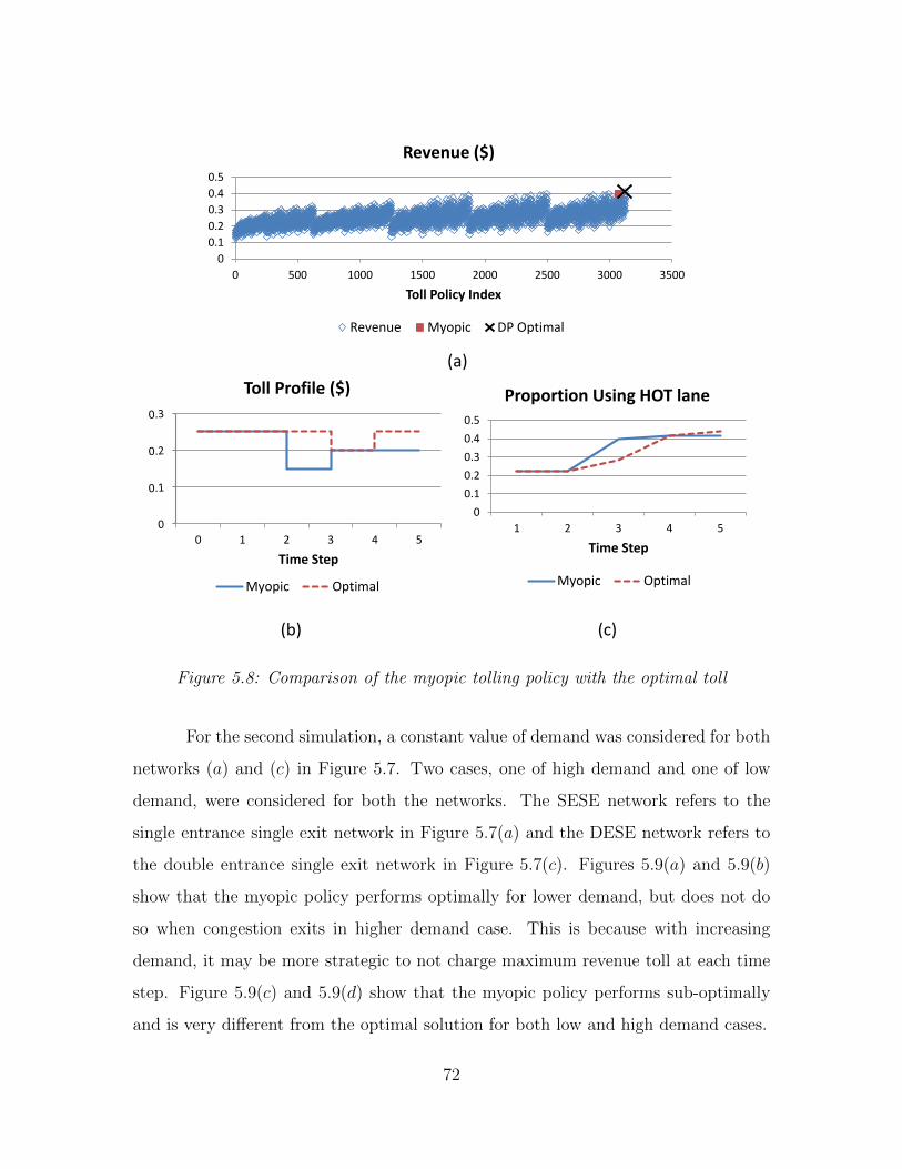
0

0.1

0.2

0.3

0.4

0.5

0 500 1000 1500 2000 2500 3000 3500

Toll Policy Index

Revenue ($)

Revenue Myopic DP Optimal

(a)

0

0.1

0.2

0.3

0.4

0.5

1 2 3 4 5

Time Step

Proportion Using HOT lane

Myopic Optimal

0 1 2 3 4 5

Time Step

Toll Profile ($)

Myopic Optimal

(b) (c)

Figure 5.8: Comparison of the myopic tolling policy with the optimal toll

For the second simulation, a constant value of demand was considered for both

networks (a) and (c) in Figure 5.7. Two cases, one of high demand and one of low

demand, were considered for both the networks. The SESE network refers to the

single entrance single exit network in Figure 5.7(a) and the DESE network refers to

the double entrance single exit network in Figure 5.7(c). Figures 5.9(a) and 5.9(b)

show that the myopic policy performs optimally for lower demand, but does not do

so when congestion exits in higher demand case. This is because with increasing

demand, it may be more strategic to not charge maximum revenue toll at each time

step. Figure 5.9(c) and 5.9(d) show that the myopic policy performs sub-optimally

and is very different from the optimal solution for both low and high demand cases.

72

This indicates that the proximity of myopic policy to the optimal performance

depends on the type of network and the level of demand. For low demand and simple

networks like Figure 5.7(a), it is possible that the myopic policy predicts the optimal

solution. However, as networks complicate and as congestion develops in the network,

the myopic policy can not be trusted for the optimal solution.

0

0.1

0.2

0.3

0.4

0 1000 2000 3000 4000

Toll Profile Index

Revenue ($) SESE Low Demand

Revenue Myopic Dp Optimal

0

0.1

0.2

0.3

0.4

0.5

0 1000 2000 3000 4000

Toll Profile Index

Revenue ($) SESE High Demand

Revenue Myopic DP Optimal

0

0.1

0.2

0.3

0.4

0.5

0 1000 2000 3000 4000

Toll Profile Index

Revenue ($) DESE Low Demand

Revenue Myopic DP Optimal

0

0.1

0.2

0.3

0.4

0.5

0.6

0 1000 2000 3000 4000

Toll Profile Index

Revenue ($) DESE High Demand

Revenue Myopic DP Optimal

(a) (b)

(c) (d)

Figure 5.9: Performance of myopic tolling for high and low values of demand

5.3 Summary

The primary objective of this chapter was to demonstrate the performance of

the dynamic programming algorithm on different test networks. The algorithm was

found to produce optimal result; however, its performance on medium to large size

73

networks was found insufficient to consider this algorithm for practical use. It was also

demonstrated that the logit model with higher value of θ performs more realistically

(in comparison to the VOT distribution performance) than the lower values of θ by

placing less weight on the randomness associated with the utility of each route. The

performance of the myopic policy for revenue maximization was also shown to depend

on the chosen network and the chosen level of demand.

The analysis in this chapter provides a background and direction for the future

work in the direction of determining optimal tolls for medium to large scale HOT

networks with multiple entrance and exits. The challenges and the future work are

discussed in more detail in the next chapter.

74

Chapter 6

Conclusions and Future Scope

6.1 Conclusions

Managed lane systems offer an alternative to alleviate congestion by providing

reliable travel time to travelers. However, as the networks involving managed lanes

continue to grow in size and complexity, there is a need to understand how dynamic

tolling can be utilized in better ways to achieve optimal objectives for the system.

Determining optimal dynamic prices for HOT lanes with multiple entrances and exits

was one of the primary motivation for the thesis. The work focused on two aspects:

(a) utilizing the real-time traffic measurements in informed decision making for pricing

of a single entrance single exit managed lane and (b) developing a methodology to

determine optimal tolls for a HOT system with multiple entrances and exits.

Chapter 3 focused on the first contribution of this work, where a non-linear

estimation model was developed to estimate the parameters for the value of time

distribution in real-time using the loop detector data. It was found that the estimated

values converge to the true values of the parameters; however, the convergence rate

depends on the choice of initial conditions, which determine when the measurements

become observable enough for the estimation to be performed. The primary result

was a framework for how real-time traffic measurements can be utilized to inform the

toll pricing in an optimal manner with simultaneous estimation of the parameters of

the model. This study, along with others in the literature, like Michalaka et al. [16]

and Lou et al. [3], provide a background on developing robust pricing models for

HOT lanes that rely less on assumptions made about the demand and driver choice;

instead, the model learns the parameters needed for determining the optimal toll from

75

the loop detector data in real-time.

Chapters 4 and 5 focused on the second contribution of this thesis, where an

optimization problem was framed for determining optimal tolls for a HOT network

with multiple entrances and exits under deterministic demand conditions. The HOT

network was assumed to be more general in contrast with previous studies [29, 24]:

it was assumed that a traveler can make the choice between the HOT and the GP

lane at every diverge location and that traffic flow entering and exiting the HOT lane

impact the traffic conditions on GP lane with time. Two optimization objectives,

revenue maximization and TSTT minimization, were considered. The backward re-

cursion algorithm developed to solve the optimization problem relied on the dynamic

programming formulation of the problem with a simplified definition of state space

made possible by the assumption that each link in the network is unit time step

long. The additional experiments conducted on different test networks highlighted

the computational limitation of the proposed algorithm in solving for optimal tolls for

medium to large scale networks. The revenue maximization results were also com-

pared to the myopic tolling policy, which was found to perform sub-optimally but

very similarly to the optimal policy predicted by the DP algorithm in the case of a

HOT network with a single entrance and exit.

6.2 Future Work

The current modeling techniques suffer from a lot of challenges; addressing

these will be the primary future work.

For the problem of estimating real-time parameters of VOT distribution, the

following aspects can be addressed as part of the future work:

1. Developing accurate methods to model the errors in loop detector readings:

The primary assumption made in most of the estimation problems using loop

detector data is that the errors involved are Gaussian with known variance. De-

76

veloping methods for dealing with cases when the errors do not have a particular

form remains a primary challenge for the field of utilizing real-time measure-

ments.

2. Developing a toll update model for others objectives like revenue maximization,

which rely not just on the current loop detector measurements, but also depend

on the detector measurements in the past and the predicted measurements in

the future.

3. Developing a day-to-day pricing model, where loop detector readings from the

previous day are combined with the current day measurements, to handle the

optimization of complicated objectives.

For the problem of solving optimal tolls for a network with multiple entrances

and exits, the biggest issue is with the computational tractability of the model. Fur-

ther research needs to be completed to develop better methods to solve the dynamic

programming formulation on real sized networks. Approximate dynamic program-

ming [51] is one such tool that will be explored in future research. Additional areas

of improvement that will constitute part of the future work include:

1. Capturing realistic traffic parameters (like capacity, jam density etc.) and test-

ing the algorithm on a medium to a large scale network

2. Handling multiple origins and destinations and non-deterministic demand

3. Extending the optimization problem to include toll sensitivity constraints

4. Extending the modeling to a VOT distribution based lane choice model captur-

ing the transformation of the VOT distribution at each decision point

77

Bibliography

[1] NCHRP, “Introducing the NCHRP 15-49 implementation guide,” in 15th Inter-

national Conference on Managed Lanes, no. S-13, 2016.

[2] D. Michalaka, J. Lu, and Y. Yin, “Fine-tuning pricing algorithms for high-

occupancy/toll (HOT) lanes,” in Transportation Research Board 92nd Annual

Meeting, no. 13-3992, 2013.

[3] Y. Lou, Y. Yin, and J. A. Laval, “Optimal dynamic pricing strategies for high-

occupancy/toll lanes,” Transportation Research Part C: Emerging Technologies,

vol. 19, no. 1, pp. 64–74, 2011.

[4] D. Schrank, B. Eisele, and T. Lomax, “TTI 2012 Urban mobility report,” Texas

A&M Transportation Institute. The Texas A&M University System, 2012.

[5] OECD, “Improving reliability on surface transport networks.” http:

//www.itf-oecd.org/sites/default/files/docs/10reliability.pdf, Ac-

cessed July 2016.

[6] FHWA, “Managed lanes: A primer,” Federal Highway Administration, US Dept.

of Transp., Washington DC, USA, 2013.

[7] E. Regan, “Managed lanes: A popular and effective urban solution,” in 2014

Global Summit: Innovations and Technologies for Sustainable Mobility, Envi-

ronment and Road Safety, 2014.

[8] LBJ, “LBJ express FAQs.” http://www.lbjtexpress.com/faq-page#

t74n1302, 2016. Accessed July 2016.

[9] A. C. Pigou, “The economics of welfare, 1920,” McMillan&Co., London, 1932.

78

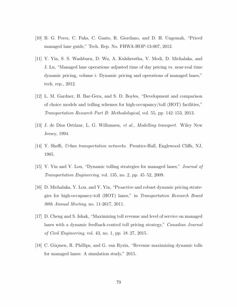
[10] B. G. Perez, C. Fuhs, C. Gants, R. Giordano, and D. H. Ungemah, “Priced

managed lane guide,” Tech. Rep. No. FHWA-HOP-13-007, 2012.

[11] Y. Yin, S. S. Washburn, D. Wu, A. Kulshrestha, V. Modi, D. Michalaka, and

J. Lu, “Managed lane operations–adjusted time of day pricing vs. near-real time

dynamic pricing, volume i: Dynamic pricing and operations of managed lanes,”

tech. rep., 2012.

[12] L. M. Gardner, H. Bar-Gera, and S. D. Boyles, “Development and comparison

of choice models and tolling schemes for high-occupancy/toll (HOT) facilities,”

Transportation Research Part B: Methodological, vol. 55, pp. 142–153, 2013.

[13] J. de Dios Ortuzar, L. G. Willumsen, et al., Modelling transport. Wiley New

Jersey, 1994.

[14] Y. Sheffi, Urban transportation networks. Prentice-Hall, Englewood Cliffs, NJ,

1985.

[15] Y. Yin and Y. Lou, “Dynamic tolling strategies for managed lanes,” Journal of

Transportation Engineering, vol. 135, no. 2, pp. 45–52, 2009.

[16] D. Michalaka, Y. Lou, and Y. Yin, “Proactive and robust dynamic pricing strate-

gies for high-occupancy-toll (HOT) lanes,” in Transportation Research Board

90th Annual Meeting, no. 11-2617, 2011.

[17] D. Cheng and S. Ishak, “Maximizing toll revenue and level of service on managed

lanes with a dynamic feedback-control toll pricing strategy,” Canadian Journal

of Civil Engineering, vol. 43, no. 1, pp. 18–27, 2015.

[18] C. Gocmen, R. Phillips, and G. van Ryzin, “Revenue maximizing dynamic tolls

for managed lanes: A simulation study,” 2015.

79

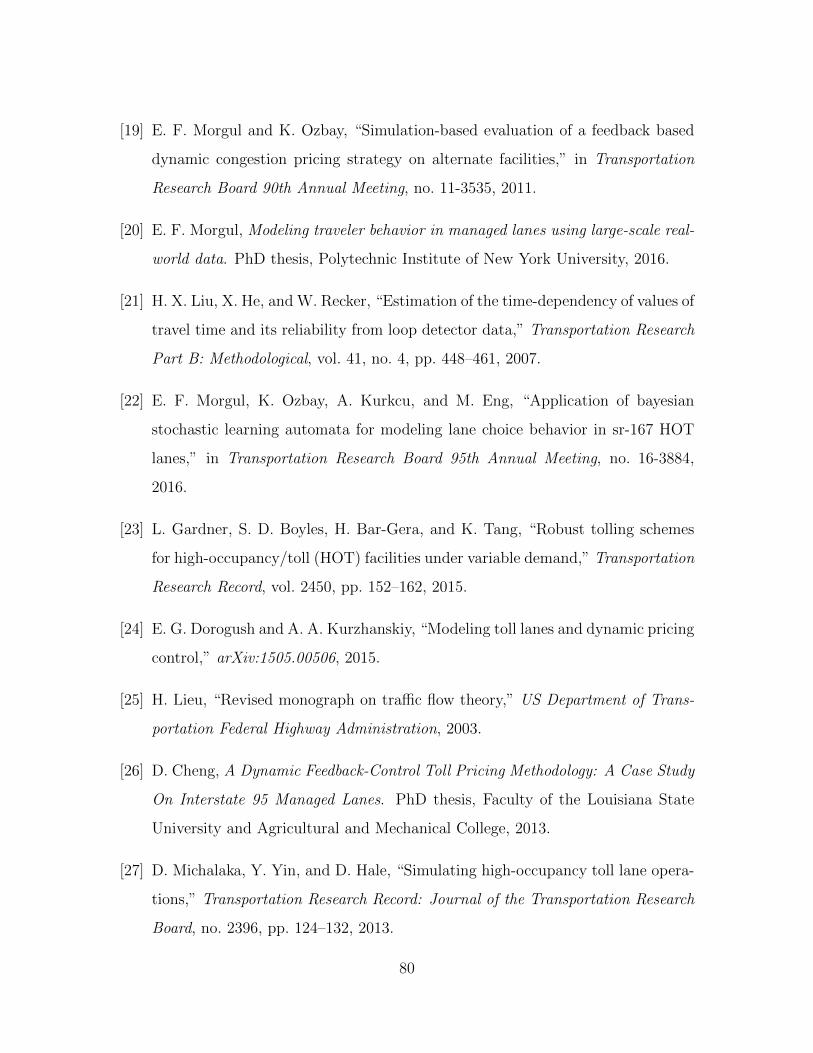
[19] E. F. Morgul and K. Ozbay, “Simulation-based evaluation of a feedback based

dynamic congestion pricing strategy on alternate facilities,” in Transportation

Research Board 90th Annual Meeting, no. 11-3535, 2011.

[20] E. F. Morgul, Modeling traveler behavior in managed lanes using large-scale real-

world data. PhD thesis, Polytechnic Institute of New York University, 2016.

[21] H. X. Liu, X. He, and W. Recker, “Estimation of the time-dependency of values of

travel time and its reliability from loop detector data,” Transportation Research

Part B: Methodological, vol. 41, no. 4, pp. 448–461, 2007.

[22] E. F. Morgul, K. Ozbay, A. Kurkcu, and M. Eng, “Application of bayesian

stochastic learning automata for modeling lane choice behavior in sr-167 HOT

lanes,” in Transportation Research Board 95th Annual Meeting, no. 16-3884,

2016.

[23] L. Gardner, S. D. Boyles, H. Bar-Gera, and K. Tang, “Robust tolling schemes

for high-occupancy/toll (HOT) facilities under variable demand,” Transportation

Research Record, vol. 2450, pp. 152–162, 2015.

[24] E. G. Dorogush and A. A. Kurzhanskiy, “Modeling toll lanes and dynamic pricing

control,” arXiv:1505.00506, 2015.

[25] H. Lieu, “Revised monograph on traffic flow theory,” US Department of Trans-

portation Federal Highway Administration, 2003.

[26] D. Cheng, A Dynamic Feedback-Control Toll Pricing Methodology: A Case Study

On Interstate 95 Managed Lanes. PhD thesis, Faculty of the Louisiana State

University and Agricultural and Mechanical College, 2013.

[27] D. Michalaka, Y. Yin, and D. Hale, “Simulating high-occupancy toll lane opera-

tions,” Transportation Research Record: Journal of the Transportation Research

Board, no. 2396, pp. 124–132, 2013.

80

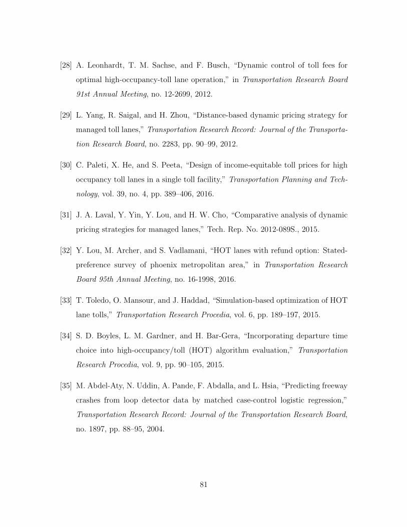
[28] A. Leonhardt, T. M. Sachse, and F. Busch, “Dynamic control of toll fees for

optimal high-occupancy-toll lane operation,” in Transportation Research Board

91st Annual Meeting, no. 12-2699, 2012.

[29] L. Yang, R. Saigal, and H. Zhou, “Distance-based dynamic pricing strategy for

managed toll lanes,” Transportation Research Record: Journal of the Transporta-

tion Research Board, no. 2283, pp. 90–99, 2012.

[30] C. Paleti, X. He, and S. Peeta, “Design of income-equitable toll prices for high

occupancy toll lanes in a single toll facility,” Transportation Planning and Tech-

nology, vol. 39, no. 4, pp. 389–406, 2016.

[31] J. A. Laval, Y. Yin, Y. Lou, and H. W. Cho, “Comparative analysis of dynamic

pricing strategies for managed lanes,” Tech. Rep. No. 2012-089S., 2015.

[32] Y. Lou, M. Archer, and S. Vadlamani, “HOT lanes with refund option: Stated-

preference survey of phoenix metropolitan area,” in Transportation Research

Board 95th Annual Meeting, no. 16-1998, 2016.

[33] T. Toledo, O. Mansour, and J. Haddad, “Simulation-based optimization of HOT

lane tolls,” Transportation Research Procedia, vol. 6, pp. 189–197, 2015.

[34] S. D. Boyles, L. M. Gardner, and H. Bar-Gera, “Incorporating departure time

choice into high-occupancy/toll (HOT) algorithm evaluation,” Transportation

Research Procedia, vol. 9, pp. 90–105, 2015.

[35] M. Abdel-Aty, N. Uddin, A. Pande, F. Abdalla, and L. Hsia, “Predicting freeway

crashes from loop detector data by matched case-control logistic regression,”

Transportation Research Record: Journal of the Transportation Research Board,

no. 1897, pp. 88–95, 2004.

81

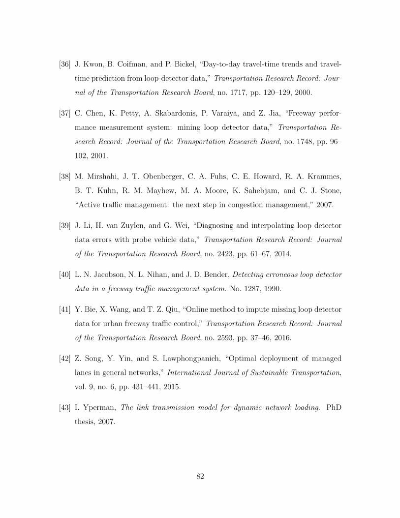
[36] J. Kwon, B. Coifman, and P. Bickel, “Day-to-day travel-time trends and travel-

time prediction from loop-detector data,” Transportation Research Record: Jour-

nal of the Transportation Research Board, no. 1717, pp. 120–129, 2000.

[37] C. Chen, K. Petty, A. Skabardonis, P. Varaiya, and Z. Jia, “Freeway perfor-

mance measurement system: mining loop detector data,” Transportation Re-

search Record: Journal of the Transportation Research Board, no. 1748, pp. 96–

102, 2001.

[38] M. Mirshahi, J. T. Obenberger, C. A. Fuhs, C. E. Howard, R. A. Krammes,

B. T. Kuhn, R. M. Mayhew, M. A. Moore, K. Sahebjam, and C. J. Stone,

“Active traffic management: the next step in congestion management,” 2007.

[39] J. Li, H. van Zuylen, and G. Wei, “Diagnosing and interpolating loop detector

data errors with probe vehicle data,” Transportation Research Record: Journal

of the Transportation Research Board, no. 2423, pp. 61–67, 2014.

[40] L. N. Jacobson, N. L. Nihan, and J. D. Bender, Detecting erroneous loop detector

data in a freeway traffic management system. No. 1287, 1990.

[41] Y. Bie, X. Wang, and T. Z. Qiu, “Online method to impute missing loop detector

data for urban freeway traffic control,” Transportation Research Record: Journal

of the Transportation Research Board, no. 2593, pp. 37–46, 2016.

[42] Z. Song, Y. Yin, and S. Lawphongpanich, “Optimal deployment of managed

lanes in general networks,” International Journal of Sustainable Transportation,

vol. 9, no. 6, pp. 431–441, 2015.

[43] I. Yperman, The link transmission model for dynamic network loading. PhD

thesis, 2007.

82

[44] T. C. Lam and K. A. Small, “The value of time and reliability: measurement

from a value pricing experiment,” Transportation Research Part E: Logistics and

Transportation Review, vol. 37, no. 2, pp. 231–251, 2001.

[45] M. Ben-Akiva, D. Bolduc, and M. Bradley, Estimation of travel choice models

with randomly distributed values of time. No. 1413, 1993.

[46] Y. Bar-Shalom, X. R. Li, and T. Kirubarajan, Estimation with applications to

tracking and navigation: theory algorithms and software. John Wiley & Sons,

2004.

[47] X. Nie and H. Zhang, “The formulation of a link based dynamic network loading

model considering queue spillovers,” tech. rep., Department of Civil and En-

vironmental Engineering, University of California, Davis, 2002. Working Paper

UCD-ITS-Zhang-2002-6, 2002.

[48] C. F. Daganzo, “The cell transmission model, part II: network traffic,” Trans-

portation Research Part B: Methodological, vol. 29, no. 2, pp. 79–93, 1995.

[49] A. K. Ziliaskopoulos, “A linear programming model for the single destination

system optimum dynamic traffic assignment problem,” Transportation science,

vol. 34, no. 1, pp. 37–49, 2000.

[50] D. P. Bertsekas, Dynamic programming and optimal control, vol. 1. Athena

Scientific Belmont, MA, 1995.

[51] W. B. Powell, Approximate Dynamic Programming: Solving the curses of dimen-

sionality, vol. 703. John Wiley & Sons, 2007.

83