Copyright

by

Monica Torres

2002

The Dissertation Committee for Monica TorresCertifies that this is the approved version of the following dissertation:

Plane-like minimal surfaces in periodic media with

inclusions

Committee:

Luis A. Caffarelli, Supervisor

William Beckner

Leszek Demkowicz

Irene Gamba

Ralph Showalter

Plane-like minimal surfaces in periodic media with

inclusions

by

Monica Torres, B.S.,M.S.

DISSERTATION

Presented to the Faculty of the Graduate School of

The University of Texas at Austin

in Partial Fulfillment

of the Requirements

for the Degree of

DOCTOR OF PHILOSOPHY

THE UNIVERSITY OF TEXAS AT AUSTIN

May 2002

Dedicated to TP.

Acknowledgments

I wish to thank to my advisor Professor Luis A. Caffarelli, to whom

I am indebted for many years of support and guidance, and also for leading

me into the area of partial differential equations. Also, I am very grateful

to Professor Rafael de la Llave for his encouragement and useful disscutions

during my thesis work. I also express my gratitude to Professor Lawrence C.

Evans for many interesting discussions, and for providing me with a great deal

of insight towards the understanding of partial differential equations.

Finally I would like to thank Professor William Beckner for his advice

during the first stages of my studies and Professor Leszek Demkowicz for the

use of the finite element codes 2Dhp90 and 3Dhp90.

I am also thankful to Tim Walsh for his support during my graduate

studies.

v

Plane-like minimal surfaces in periodic media with

inclusions

Publication No.

Monica Torres, Ph.D.

The University of Texas at Austin, 2002

Supervisor: Luis A. Caffarelli

The mathematical areas of minimal surfaces and homogenization of PDE have

been subjects of research for many decades. In this work we consider the

particular case of minimal surfaces in heterogeneous media. We prove theoret-

ical results and develop numerical algorithms that characterize the behavior

of these surfaces. We also show that this work turns out to be related to the

theory of homogenization of Hamilton-Jacobi equations.

In this work we think of Rn as a lattice of points with integer coor-

dinates, where each cube of edge length 1 has an internal inclusion (we can

think of an inclusion as a hole or as a part of the domain containing another

material). All inclusions are compact and periodic. Within this framework we

measure the area of a surface of codimension one by neglecting the parts that

are inside the inclusions, and measuring the outside parts in the standard way.

We say that the surface is a minimal surface if any compact perturbation of it

increases the area (in this degenerate metric).

vi

In this work we prove the existence of minimal surfaces that always

stay at a bounded distance (universal) from a given hyperplane. While we

know that the surface is smooth outside the inclusions, in this work we prove

a result concerning the behaviour of the minimal surfaces at the boundary:

that the intersection between the inclusions and the surface locally looks like

two perpendicular hyperplanes.

Within this degenerate metric, the smallest distance between two points

is no longer a line. We analyze the behavior of this distance when the edge

length of the cube goes to zero. In particular, we want to find, for the case n =

2 and the inclusions being closed balls, the effective norm in the homogenized

limit. The effective norm depends on the radius of the inclusions, and our

results suggest that as the radius gets smaller the behavior of the effective

norm changes, though it is always polygonal with more and more sides, until

it becomes a circle in the limit.

We implement an algorithm to compute our weighted minimal surfaces.

We extend the Bence-Merriman-Osher algorithm to the case of heterogeneous

domains. We implement the algorithm in 2 and 3 dimensions using adaptive

finite element methods.

vii

Table of Contents

Acknowledgments v

Abstract vi

List of Tables x

List of Figures xi

Chapter 1. Introduction 1

1.1 Introduction . . . . . . . . . . . . . . . . . . . . . . . . . . . . 1

Chapter 2. Proof of Theorem 1. 7

2.1 Main definitions and existence of minimizers . . . . . . . . . . 7

2.2 Infimal minimizer . . . . . . . . . . . . . . . . . . . . . . . . . 13

2.3 Birkhoff property . . . . . . . . . . . . . . . . . . . . . . . . . 17

2.4 The case when ω is not rational . . . . . . . . . . . . . . . . . 20

2.5 Proof of Theorem 1 . . . . . . . . . . . . . . . . . . . . . . . . 21

Chapter 3. Homogenization for n=2. 39

3.1 Homogenization for the case n = 2 . . . . . . . . . . . . . . . . 39

3.2 Connection with Effective Hamiltonians . . . . . . . . . . . . . 50

Chapter 4. An algorithm to compute weighted minimal surfacesin 2 and 3 dimensions. 61

4.1 Preliminaries . . . . . . . . . . . . . . . . . . . . . . . . . . . . 61

4.2 The Algorithm . . . . . . . . . . . . . . . . . . . . . . . . . . . 63

4.3 Numerical implementation . . . . . . . . . . . . . . . . . . . . 68

4.4 Results . . . . . . . . . . . . . . . . . . . . . . . . . . . . . . . 70

Bibliography 84

viii

Vita 88

ix

List of Tables

x

List of Figures

2.1 Diagram showing parallel plane restrictions and period for min-imization. . . . . . . . . . . . . . . . . . . . . . . . . . . . . . 10

2.2 Case when C ⊂ Rn\E . . . . . . . . . . . . . . . . . . . . . . . 18

2.3 Case when C ⊂ E . . . . . . . . . . . . . . . . . . . . . . . . . 19

3.1 n ≤ m, n ≥ 1 . . . . . . . . . . . . . . . . . . . . . . . . . . . 41

3.2 Unit balls for limiting norms. P = R = ( 1√2−2ρ

, 1√2−2ρ

), Q =

( 1√5−2ρ

, 2√5−2ρ

), S = ( 2√5−2ρ

, 1√5−2ρ

). . . . . . . . . . . . . . . . 48

4.1 Diagram showing the domain with inclusions where we are solv-ing the equation 4.2.9 . . . . . . . . . . . . . . . . . . . . . . . 69

4.2 A 2-Dimensional h-adaptive finite element simulation of motionby weighted mean curvature. The initial surface was a straightline parallel and close to the bottom of the domain. The grid inthe figure is the mesh used to solve the PDE. The parametersare: mod=6, ∆t = 0.01, iter=100, b=0.1 . . . . . . . . . . . . 73

4.3 A 2-Dimensional h-adaptive finite element simulation of motionby weighted mean curvature. The initial surface was a straightline parallel and close to the bottom of the domain. The grid inthe figure is the mesh used to solve the PDE. The parametersare mod = 12, ∆t = 0.01, iter=100, b=0.1 . . . . . . . . . . . 74

4.4 A 2-Dimensional h-adaptive finite element simulation of motionby weighted mean curvature. The initial surface was a straightline parallel and close to the bottom of the domain. The gridin the figure is the mesh used to solve the PDE. Compare thisresult with the next one, which only contains the diffusion term.Compare also with Figure 4.2, in which we performed 100 iter-ations instead of 25. The parameters are: mod=6, ∆t = 0.01,iter=25, b=0.1 . . . . . . . . . . . . . . . . . . . . . . . . . . 75

4.5 A 2-Dimensional h-adaptive finite element simulation of motionby weighted mean curvature. The initial surface was a straightline parallel and close to the bottom of the domain. The gridin the figure is the mesh used to solve the PDE. This examplecontains only the diffusion term. The parameters are: mod=6,∆t = 0.01, iter=25, b=0.1 . . . . . . . . . . . . . . . . . . . . 76

xi

4.6 A 2-Dimensional h-adaptive finite element simulation of motionby weighted mean curvature. The initial surface was a straightline parallel and close to the bottom of the domain. The grid inthe figure is the mesh used to solve the PDE. Note the refine-ment of the mesh around the inclusions. The parameters are:mod=8, ∆t = 0.01, iter=100, b=0.05 . . . . . . . . . . . . . . 77

4.7 A 2-Dimensional h-adaptive finite element simulation of motionby weighted mean curvature. The initial surface was a straightline parallel and close to the bottom of the domain. This sim-ulation contains only the diffusion term. The grid in the fig-ure is the mesh used to solve the PDE. Note the refinement ofthe mesh around the inclusions. The parameters are: mod=8,∆t = 0.01, iter=100, b=0.05 . . . . . . . . . . . . . . . . . . . 78

4.8 A 2-Dimensional h-adaptive finite element simulation of motionby weighted mean curvature. The initial surface was a straightline parallel and close to the bottom of the domain. The grid inthe figure is the mesh used to solve the PDE. Note the refine-ment of the mesh around the inclusions. The parameters are:mod=8, ∆t = 0.01, iter=250, b=0.1 . . . . . . . . . . . . . . . 79

4.9 A 2-Dimensional h-adaptive finite element simulation of motionby weighted mean curvature. The initial surface was a straightline parallel and close to the bottom of the domain. The grid inthe figure is the mesh used to solve the PDE. Note the refine-ment of the mesh around the inclusions. The parameters are:mod=4, ∆t = 0.01, iter=250, b=0.1 . . . . . . . . . . . . . . . 80

4.10 A 2-Dimensional h-adaptive finite element simulation of motionby weighted mean curvature. The initial surface was a straightline parallel and close to the bottom of the domain. This sim-ulation contains only the diffusion term. The grid in the fig-ure is the mesh used to solve the PDE. Note the refinement ofthe mesh around the inclusions. The parameters are: mod=8,∆t = 0.01, iter=250, b=0.1 . . . . . . . . . . . . . . . . . . . . 81

4.11 A 2-Dimensional h-adaptive finite element simulation of motionby weighted mean curvature. The initial surface was a straightline parallel and close to the bottom of the domain. The grid inthe figure is the mesh used to solve the PDE. Note the refine-ment of the mesh around the inclusions. The parameters are:mod=16, ∆t = 0.005, iter=500, b=0.1 . . . . . . . . . . . . . 82

xii

4.12 A 3-Dimensional h-adaptive finite element simulation of motionby weighted mean curvature. The initial surface was a planeparallel and close to the bottom of the domain. We are showingtwo different views of the same evolution. For clarity we onlyshow the surface and the elements of the mesh that form theinclusions. The parameters are: mod=6, ∆t = 0.01, iter=350(we start sharpening after the first 100 iterations), b=0.02 . . 83

xiii

Chapter 1

Introduction

1.1 Introduction

In [10], Luis Caffarelli and Rafael de la Llave consider minimizers of

periodic geometric variational problems on sets of locally finite perimeter in

Rn and other manifolds. These problems include as a particular case the

problem of finding hypersurfaces of codimension one of minimal area. More

specifically, they study minimizers of the elliptic integral:

J(E) =

∫F (x, ν)|DϕE|

over a class of periodic closed Cacciopoli sets (sets of finite perimeter) that

contain a semispace. The measure |DϕE| is the total variation of the vector

valued Radon measure DϕE (which is the gradient of ϕE , the characteristic

function of E, in the sense of distributions). If ∂E is C2, |DϕE| is simply the (n-

1)-dimensional Hausdorff measure Hn−1. F satisfies the following properties,

among others: it is continuous, convex and homogeneous of degree 1 in the

second variable ν, periodic in x and non-degenerate (λ ≤ F (x, ν) ≤ Λ). They

prove that there are minimizers that stay at a bounded distance from a given

plane. This distance is bounded a priori by properties of the metric and

1

independently of the plane. If we take F (x, ν) = |ν|, [10] includes the case of

minimal surfaces for smooth metrics on Rn and in other manifolds.

The problem of constructing minimal surfaces for periodic metrics was

proposed in [26], where similar results are proven for minimizers of a similar

(but different) class of those that are considered in [10]. In [26] the connection

of these results with the Aubry-Mather theory is shown. Also, [2] contains

part of the results (presented in the context of geometric measure theory)

proven in [10] for minimal surfaces in Tn with a Riemannian metric.

In this thesis, we extend [10] and consider the case of a degenerate

metric. We also work in the context of sets of finite perimeter, and therefore

we deal with boundaries of sets. This is useful since we do no need to consider

aspects of orientability. Also, this allow us to take inclusions of sets.

Another goal of this thesis is to begin exploring the connections of this

theory with the theory of homogenization.

In what follows we consider Rn as a lattice of cubes. We assume that

each cube of edge length 1 has an internal inclusion (an inclusion can be a hole

or a part of the domain containing another material). Let Y be a fundamental

cube, that is, a cube of edge length 1 and vertices with integer coordinates.

Let Z be the inclusion inside Y. We assume:

1. Z is compact.

2. ∂Z ∩ ∂Y = ∅

2

Any other inclusion is an integer translation of Z. We denote α =

d(∂Z, ∂Y ).

Let Σ be a surface in Rn of codimension 1. We consider the following

procedure for measuring the area of Σ: the parts that are inside the inclusions

do not contribute to the area, but outside the inclusions the area is measured in

the standard way. Let Rni denote Rn with this way of measuring area. We say

that Σ is a minimal surface in Rni if Σ minimizes area outside the inclusions.

(This is made precise in Section 2).

The next two chapters of the thesis are devoted to constructing plane-

like minimal surfaces in Rni ; that is, minimal surfaces that stay at a bounded

distance (universal) from a plane. We say that a constant C is universal if it

only depends on the dimension n and α. More precisely, the theorem we prove

is:

Theorem 1. There exists a universal constant C, such that for every (n-1)-

dimensional hyperplane Π, we can find a minimal surface Σ in Rni such that

d(Π, Σ) ≤ C. The surface Σ is the boundary of a set that includes a semispace

bounded by Π. Moreover, if n ≤ 6 and the inclusions have C2 boundary, Σ

enters the inclusions orthogonally.

In Theorem 1, by orthogonal we mean that the intersection of Σ with

an inclusion looks like two perpendicular hyperplanes when viewed locally.

Mathematically, this means that we can trap Σ in a cone forming an arbitrarily

small angle θ such that as θ goes to zero, the cone tends to a hyperplane

3

perpendicular to the inclusion.

The surface Σ given by Theorem 1 will be periodic when the slope of

the given hyperplane is rational. If the slope of the hyperplane is irrational we

will see that we can approximate with rational slopes but in this case Σ will

not be periodic.

The first part of Theorem 1 is true for any dimension and for inclusions

satisfying the two conditions given at the beginning of the introduction. The

second part of Theorem 1 will be proven when the inclusions have C2 boundary

and n ≤ 6. The orthogonallity will be clearly true for n=2, since as we will

see in the last section, for this case Σ consists of pieces of lines connecting

inclusions.

For the first part of Theorem 1 the main tool is the density estimates

that minimizers satisfy. The existence of minimizers is given by a lower semi-

continuity. Moreover, due to some subadditivity properties, it is possible to

define an infimal minimizer which is contained in all the other minimizers.

The infimal minimizer satisfies several monotonicity properties including a ge-

ometric property analogous to the property called Birkhoff in Aubry-Mather

theory. This property, together with the density estimates allow us to prove

that the infimal minimizer is contained in a band whose width is independent

of the direction of the plane. A similar theorem to the first part of Theorem

1 is proven in [10], for C2 metrics on Rn and in other manifolds.

The second part of Theorem 1 is obtained by blowing up the minimizer

4

around a point of its boundary that lies on the boundary of an inclusion. The

main point here is that we can prove also the density estimates for points on the

boundary of the minimizer that lie on the boundary of the inclusions. These

density estimates allow us to pass to the limit and obtain (after a suitable

reflection) a minimal cone. We then use the well known theorem concerning

the non-existence of minimal cones for dimension n ≤ 7. (See [28], [18]).

Later in the dissertation we begin to explore the connections with ho-

mogenization. Indeed, in some sense Theorem 1 tell us that, in spite of our

heterogeneous media, the infimal minimizer looks like a plane (homogeneos

media) when seen from a far distance. We know that the smallest distance

between two points in R2 is given by the line that joins the two points. How-

ever, in R2i this might not be the case. For example, considering the particular

case where the inclusions are closed balls with radius ρ, we can prove that if

ρ > 2−√22

, the smallest distance in R2i between two points that are centers of

balls is given by a path that consists only of vertical and horizantal segments.

An interesting question is to study the behavior of our minimal surfaces

when we fix two points in the plane and let the edge length of the cubes tend

to zero. If P and Q denote any two fixed points in the plane and dρε (P, Q)

denotes the smallest distance between P and Q (this length measured in R2i )

at the scale ε ( that is, when the size of the cubes is ε and the radius of

the inclusions is ρε) then the limit dρ0(P, Q) := limε→0 dρ

ε (P, Q) will be called

the homogenized limit. The function dρ0 defines a norm and will be called the

effective norm. In particular, we want to find, for the case n = 2, the effective

5

norms for different values of ρ.

Let | · |1 and | · |2 denote the l1 and Euclidean norms in R2 respectively.

In the last section we prove that the effective norm is (1− 2ρ)| · |1 (if ρ is big

enough). As ρ decreases, we get other effective norms, but our results suggest

that they (unit balls) are polygons with more and more edges. Also, we prove

that the effective norms converge to | · |2 as ρ goes to zero.

6

Chapter 2

Proof of Theorem 1.

2.1 Main definitions and existence of minimizers

We first recall some theory regarding sets of finite perimeter. Let Ω ⊂Rn be an open set and let f ∈ L1(Ω). Define:∫

Ω

|Df | = sup∫

Ω

fdivg : g ∈ C10(Ω; Rn), |g(x)| ≤ 1, for x ∈ Ω

A function f ∈ L1(Ω) is said to have bounded variation in Ω if∫Ω|Df | <

∞. We define BV (Ω) as the space of all functions in L1(Ω) with bounded

variation. With the norm |f |BV = |f |L1(Ω) +∫Ω|Df |, BV (Ω) is a Banach

space.

Let E be a Borel set. Define the perimeter of E in Ω as:

Per(E, Ω) =

∫Ω

|DϕE|

where ϕE is the characteristic function of the set E.

If a Borel set E has locally finite perimeter, that is, if Per(E, Ω) < ∞for every bounded open set Ω, then E is called a Cacciopoli set. If E ⊂ Rn

has C2 boundary then Per(E, Ω) is the (n-1)-dimensional Hausdorff measure

of ∂E ∩ Ω; that is, Per(E, Ω) = Hn−1(∂E ∩ Ω).

7

Let fj be a sequence of functions in BV (Ω) that converge in L1loc(Ω)

to a function f. The following semicontinuity property holds:∫Ω

|Df | ≤ lim infj→∞

∫Ω

|Dfj| (2.1.1)

Since BV (Ω) ⊂ L1(Ω), it makes no sense to talk about the value of a

BV function on ∂Ω, which is a set of measure zero. To solve this problem,

given f ∈ BV (Ω), we can build a function ftr such that:

limρ→0

∫B(y,ρ)∩Ω

|f(x)| = ftr(y)

for every y ∈ ∂Ω. ftr is called the trace function.

Finally, we define the reduced boudary of a Cacciopoli set E, which play

a fundamental role in the regularity theory (See [18]). We say that x ∈ ∂E is

a point in the reduced boundary if:

• ∫B(x,ρ)

|DϕE| > 0 for all ρ > 0.

• The limit ν(x) = limρ→0+

∫B(x,ρ)

DϕE/|DϕE| exists.

• |ν(x)| = 1.

The reduced boundary is usually denoted by ∂∗E. An important fact

is that ∂∗E is dense in ∂E. Details about theory of Cacciopoli sets can be

found in [16, 18].

8

Let O = Rn\Inclusions. We make the following definitions:

We say that the Cacciopoli set E ⊂ Rn has least area or perimeter in

Ω if∫Ω

|DϕE| = inf∫

Ω

|DϕF | : F is a Cacciopoli set, spt(ϕF − ϕE) ⊂ Ω

We say that the Cacciopoli set E ⊂ Rn is a class A minimizer if it has least

area in B(0, R) ∩ O, where B(0, R) is any open ball. In other words, E is

a class A minimizer if any perturbation of E inside any open ball B(0, R),

(which would be a new set L that has the same trace as E on ∂B(0, R)) results

in the property that Per(E, B(0, R) ∩O) ≤ Per(L,B(0, R) ∩ O).

Definition 2.1.1. Σ ⊂ Rn is a minimal surface in Rni if Σ = ∂E, where E is a

class A minimizer.

It is proven in [18] that, if n ≤ 7 and E is a Cacciopoli set that

has least area in Ω, then ∂E ∩ Ω is a smooth surface. At times we will use

the word “surface” to denote the boundary of a Cacciopoli set, although this

boundary could have singularities. These singularities, if ∂E minimizes area,

have (n− 8)-Hausdorff dimension zero (See also [8]).

We now start to prove the existence of minimizers. Let ω ∈ Rn. Let

us consider first the case when ω ∈ Qn. Let N ∈ Z, M ∈ R, with M, N > 0.

Define:

S1 = Γω,0 = x ∈ Rn : x · ω ≤ 0

S2 = Γω,M = x ∈ Rn : x · ω|ω| ≤ M

9

Figure 2.1: Diagram showing parallel plane restrictions and period for mini-mization.

We denote Π1 = x ∈ Rn : x · ω = 0 and Π2 = x ∈ Rn : x · ω|ω| = M

as the parellel plane restrictions. Define now:

AS1,S2 = E : E is a closed Cacciopoli set, S1 ⊂ E ⊂ S2 , TNkE = E ,

∀k ∈ Zn with ω · k = 0

Since the sets in AS1,S2 are periodic, we can minimize the perimeter

outside the inclusions in an open parellelogram P , representing one period

(Figure 1).

10

Let H1, ..., Hk be the inclusions with Hi ∩ P 6= ∅. Define I =⋃k

i=1 Hi

and set Ω = P − I. Define, for each E ∈ AS1,S2 :

J(E) =

∫Ω

|DϕE| (2.1.2)

Let β = infE∈AS1,S2J(E). Let Ej be a sequence such that J(Ej) →

β. Therefore, the sequence ∫Ω|DϕEj

| is uniformly bounded. Hence, since

BV (Ω) → L1(Ω), there exists a subsequence, that we detote again by Ej,such that Ej is convergent in L1(Ω). Let E0 ∈ L1(Ω) be the limit.

By (2.1), ∫Ω

|DϕE0| ≤ lim inf

∫Ω

|DϕEj|

Thus,

J(E0) = infE∈AS1,S2

J(E)

We make the following definitions:

Definition 2.1.2. If E ∈ AS1,S2 satisfies J(E) = J(E0) then E will be called a

minimizer corresponding to the class AS1,S2 .

Definition 2.1.3. We will say that the minimizer E is an unconstrained mini-

mizer if we can find M1, M2 ∈ R such that Γω,M1 ⊂ Int(S1), S2 ⊂ Int(Γω,M2)

and E is a minimizer corresponding to the class AT1,T2, where T1 = Γω,M1 and

T2 = Γω,M2.

11

In other words, if E is an unconstrained minimizer then the parallel

plane restrictions are irrelavant.

Let E be a minimizer corresponding to the class AS1,S2. Since S1 ⊂ E

and S1 is connected, it follows that S1 is contained in a single component of

E, say E1. Notice that J(E1) > 0 since ∂E1 ∩O 6= ∅. We now define:

Definition 2.1.4. We will say that the minimizer E is connected if E1 is the

only component satisfying J(E1) > 0.

Notice that if E has a component contained inside an inclusion, then

this component does not contribute to (2.2) at all and it can be neglected. The

following Lemma will prove that in fact the minimizer E0 constructed above

has only one component that contributes to (2.2) with a nonzero quantity.

Lemma 2.1.1. Let E be a minimizer corresponding to the class AS1,S2 . Then,

E and Rn\E are connected.

Proof: As above, let E1 denote the component of E that contains S1.

We know that J(E1) > 0. Assume that E has another component, say E2,

with J(E2) > 0. This implies that J(E1) < J(E), which contradicts the fact

that E is a minimizer. We can now consider the class AS2,S1, where S2 and

S1 interchange roles. Notice that Rn\E is a minimizer corresponding to this

class. Hence, the same argument above shows that Rn\E is connected.

Let E be a minimizer corresponding to the class AS1,S2 . Consider ∂E ∩O. It is proven in [9, 18] that for n < 8, ∂E ∩ O is locally the graph of a

smooth function. If n ≥ 8, ∂E ∩ O may have singularities, but in this case,

12

for any k > n− 8 the k-dimensional Hausdorff measures of these singularities

are zero.

2.2 Infimal minimizer

The minimizer we have just constructed may not be unique. However,

we can prove the existence of an infimal minimizer, that is, a minimizer that is

contained in any other minimizer. Clearly, if such an infimal minimizer exists,

it is unique. In order to prove its existence, we use the following theorem:

Theorem 2.2.1. Let A and B be Caccipoli sets. Let Ω be any open set. Then

Per(A ∩B, Ω) + Per(A ∪B, Ω) ≤ Per(A, Ω) + Per(B, Ω).

Proof: Let f, g be two smooth functions with 0 ≤ f ≤ 1, 0 ≤ g ≤ 1.

Define Ψ = f + g − fg and Φ = fg. Notice that:∫Ω

|DΨ| ≤∫

Ω

(1− f)|Dg|+∫

Ω

(1− g)|Df |∫Ω

|DΦ| ≤∫

Ω

f |Dg|+∫

Ω

g|Df |

This implies: ∫Ω

|DΦ|+∫

Ω

|DΨ| ≤∫

Ω

|Df |+∫

Ω

|Dg| (2.2.3)

We can find [18] sequences of smooth functions fj and gj such that fj →ϕA, gj → ϕB, in L1(Ω) and

∫Ω|Dfj| →

∫Ω|DϕA|,

∫Ω|Dgj| →

∫Ω|DϕB|. Since

Ψj = fj + gj − fjgj → ϕA∪B, Φj = fjgj → ϕA∩B, the Theorem follows from

(3.6) and (1.1).

13

Now we can prove the existence of the infimal minimizer.

Theorem 2.2.2. There exists E∗ ∈ AS1,S2, such that E∗ is the infimal minimizer

corresponding to this class.

Proof: Let B be the set of all minimizers. Let Ω be the open set defined

in section 2. We have that B ⊂ L1(Ω).

Let E1, E2 ∈ B. By theorem 3.1 we have:

Per(E1 ∩E2, Ω) + Per(E1 ∪E2, Ω) ≤ Per(E1, Ω) + Per(E2, Ω).

But Per(E1, Ω) = Per(E2, Ω). Since E1∪E2 is an admissible set, we have that:

Per(E1 ∪ E2, Ω) ≥ Per(E1, Ω)

hence:

Per(E1 ∩ E2, Ω) ≤ Per(E1, Ω)

which implies that E1∩E2 is also a minimizer. Since we can uniformly bound

the perimeters of minimizers in Ω, it follows from (1.1) that B is a compact

subset of L1(Ω). Since L1(Ω) is separable, B is also separable. Let Ej be a

dense subset of B and define:

En =

n⋂j=1

Ej

Each En is a minimizer. Since En+1 ⊂ En and |E1 ∩ Ω| < ∞ we have that:

|En ∩ Ω| → |∞⋂

n=1

En ∩ Ω|

thus,

En →∞⋂

n=1

En in L1(Ω)

14

Let

E∗ =∞⋂

n=1

En

By (1.1),

Per(E∗, Ω) ≤ lim inf Per(En, Ω)

which implies that E∗ is a minimizer.

Let E be any other minimizer. We now want to prove that |(E∗\E) ∩Ω| = 0. If this is not true, then |(E∗\E) ∩ Ω| > δ > 0. Since Ej is a dense

subset of B, we can find Ek such that |(Ek\E) ∩ Ω| < ε2, ε < δ. Choose N

large enough such that EN ⊂ Ek and |(E∗\EN ) ∩ Ω| < ε2. We have:

|(E∗\E) ∩ Ω| ≤ |(E∗\EN ) ∩ Ω| + |(EN\E) ∩ Ω|

≤ |(E∗\EN ) ∩ Ω| + |(Ek\E) ∩ Ω|

≤ ε

2+

ε

2= ε < δ

which is a contradiction. We conclude that E∗ is the infimal minimizer.

Let M1, M2 ∈ R be such that T1 := Γω,M1 ⊂ S1 and T2 := Γω,M2 ⊂ S2

, with T1 ⊂ T2. The following Proposition will be used later to establish

properties of the infimal minimizer.

Proposition 2.2.1. Let E be a minimizer corresponding to the class AS1,S2 and

L a minimizer corresponding to the class AT1,T2. Then:

(a) E ∩ L is a minimizer corresponding to the class AT1,T2.

15

(b) E ∪ L is a minimizer corresponding to the class AS1,S2.

(c) E∗,T1,T2 ⊂ E∗,S1,S2

Proof: Note that E ∪ L ∈ AS1,S2 and E ∩ L ∈ AT1,T2. Since E and L

are minimizers, we have:

Per(E, Ω) ≤ Per(E ∪ L, Ω)

Per(L, Ω) ≤ Per(E ∩ L, Ω)

Using theorem 3.1:

Per(E ∩ L, Ω) + Per(E, Ω) ≤ Per(E ∩ L, Ω) + Per(E ∪ L, Ω)

≤ Per(E, Ω) + Per(L, Ω)

⇒ Per(E ∩ L, Ω) ≤ Per(L, Ω)

This implies that E ∩L is a minimizer in the class AT1,T2 , which proves

(a). In the same way we prove (b).

In order to prove (c) notice that, by (a), E∗,T1,T2∩E∗,S1,S2 is a minimizer

corresponding to the class AT1,T2 . Hence:

E∗,T1,T2 ⊂ (E∗,T1,T2 ∩ E∗,S1,S2)

⇒ E∗,T1,T2 ⊂ E∗,S1,S2

16

2.3 Birkhoff property

Let E be the infimal minimizer corresponding to the class AS1,S2. We

will denote by Tk the translation operator by k ∈ Zn, that is, Tk(x) = x + k ,

x ∈ Rn. The Birkhoff property is stated in the following Lemma.

Lemma 2.3.1. Let k ∈ Zn.

(a) if k · ω ≤ 0 then TkE ⊂ E.

(b) if k · ω ≥ 0 then E ⊂ TkE.

In particular, if k · ω = 0, we have TkE = E.

Proof:(a) Let T1 = Tk(S1) and T2 = Tk(S2), where as before S1 = x ∈Rn : x · ω ≤ 0 and S2 = x ∈ Rn : x · ω ≤ M. If k · ω ≤ 0 we have that

T1 ⊂ S1, T2 ⊂ S2, and T1 ⊂ T2. Notice that TkE is the infimal minimizer in

AT1,T2. By Proposition 3.1 we have TkE ⊂ E.

(b)If k ·ω ≥ 0 we have that S1 ⊂ T1, S2 ⊂ T2, and T1 ⊂ T2. Again TkE

is the infimal minimizer in AT1,T2 . By Proposition 3.1, E ⊂ TkE.

In what follows we will use the word slab to denote the region in between

two hyperplanes, both parallel to the parallel plane restrictions Π1 and Π2.

We now prove the following Lemma:

Lemma 2.3.2. Let C be a cube of edge length l ≥ 3.

(a) if C ⊂ Rn\E, then there exists a slab of width at least one contained

in Rn\E.

17

>1C

p .

integer coordinates)(vetex with

width of S > 1

q .

S

=1

Figure 2.2: Case when C ⊂ Rn\E

(b) if C ⊂ E, then there exists a slab of width at least one contained in

E.

Proof: (a) Proceed by contradiction. Let S be the slab as shown in

Figure 2. Assume that there exists a point p ∈ S with p ∈ E. Then, we can

find k ∈ Zn, k ·ω ≤ 0, such that Tk(p) = q with q in the shaded region of C. By

Lemma 4.1, TkE ⊂ E. This implies that q ∈ E, which gives a contradiction.

Notice that the width of the slab S is larger than 1.

(b)Proceed again by contradiction. Let S be the slab as shown in

Figure 3. Assume that there exists p ∈ S with p ∈ Rn\E. We can find

k ∈ Zn, ω · k ≥ 0 such that Tk(p) = q, with q in the shaded region of C. Now,

ω · (−k) ≤ 0 and, by Lemma 4.1, T−kE ⊂ E. Since T−k(q) = p, this implies

that p ∈ E, which is a contradiction. Notice that the width of the slab S is

18

>1C

p .q .

width of S > 1

S(vetex with

integer coordinates)

=1

Figure 2.3: Case when C ⊂ E

larger than 1.

We will use the previous Lemma to prove the following Proposition,

which will be used in the next section to prove Theorem 1.

Proposition 2.3.1. Let C be a cube of edge length l ≥ 3. Then, we can not

have C ⊂ E\S1 where S1 = x ∈ Rn : x · ω ≤ 0.

Proof: Assume that C ⊂ E\S1. Then by Lemma 4.2, there exists a

slab of width larger than 1 contained in E. Let Π1 and Π2 be the lower and

upper hyperplanes respectively that bound this slab. Since the slab has width

larger than 1, it has to contain a point with integer coordinates that does not

intersect Π1 or Π2. Let Π be the plane that contains this point and is parallel

to Π1 and Π2. This plane Π divides E in two parts. One of this parts, say

E1, contains Π1, and the other part, say E2, contains Π2. We can find k ∈ Zn,

19

with k · ω ≤ 0, such that Tk(Π2) = Π. Let S denote the interior of the slab

in between Π and Π2. Consider now the set E1 ∪ Tk(E2\S). Clearly, this set

is also a minimizer contained (and not equal) in E. This contradicts the fact

that E is the infimal minimizer, that is, a minimizer that is contained in any

other minimizer.

2.4 The case when ω is not rational

Given ω ∈ Rn\Qn, we can construct a sequence ωj ∈ Qn with ωj →ω. Let Eωj

denote the corresponding infimal minimizers constructed as in

the previous sections. Consider B(0, R), the open ball of radius R centered at

the origin. We have:

Per(Eωj, B(0, R) ∩O) ≤ CRn−1

Thus, Eωj has a subsequence that is convergent in L1(B(0, R) ∩ O). By

applying the diagonal procedure, we get a subsequence of Eωj (which we

will denote again as Eωj) and a set Eω such that Eωj

→ Eω in L1loc(Rn ∩O).

We need to check that Eω is a class A minimizer. Let ε > 0. Consider

again the ball B(0, R) and assume that we perturb Eω inside the ball, result-

ing in a new set L. Since each Eωjis a minimizer and since Eωj

→ Eω in

L1(B(0, R) ∩ O), we have that for j large enough:

Per(Eωj, B(0, R) ∩ O) ≤ Per(L,B(0, R) ∩O) + γ(ε)

20

where γ(ε) goes to zero as ε → 0.

Using (1.1), and since Eωj→ Eω in L1(B(0, R) ∩ O), we have:

Per(Eω, B(0, R) ∩ O) ≤ lim inf Per(Eωj, B(0, R) ∩ O)

≤ Per(L,B(0, R) ∩ O) + γ(ε)

Letting ε → 0 we have

Per(Eω, B(0, R) ∩O) ≤ Per(L,B(0, R) ∩O)

This proves that Eω is a class A minimizer. Finally, since d(∂Eωj, ∂Γ0,ωj

) ≤2λ√

n it follows that d(∂Eω, ∂Γ0,ω) ≤ 2λ√

n.

2.5 Proof of Theorem 1

Let E be the infimal minimizer corresponding to the class AS1,S2. Re-

call our notation O = Rn\Inclusions. In order to clarify exposition, in the

remainder of the thesis we use the same C to denote different universal con-

stants.

The proof of the first part of Theorem 1 will be a covering argument.

We will need to prove that we can cover the boundary of E with cubes of edge

length 2 in such a way that each of these cubes contains at least some fixed

amount of area (that will depend only on the dimension and α). This is a

consequence of the following three Lemmas.

21

Lemma 2.5.1. Let x ∈ ∂E∩O. Assume that x is contained in one fundamental

cube, say Y , that does not intersect the parallel plane restrictions. Then,

∂E ∩ ∂Y 6= ∅.

Proof: If x ∈ ∂Y the proof is complete. Consider the case x ∈ Int(Y ).

Let ρ > 0 such that B(x, ρ) ⊂ Int(Y ) ∩ O. Since x ∈ ∂E and ∂∗E is dense

in ∂E, by an approximation argument and using Lemma 5.2 below we obtain∫B(x,ρ)

|DϕE| ≥ Cρn−1 > 0.

Assume that ∂E ∩ ∂Y = ∅. This implies that ∂Y ⊂ Int(E) or ∂Y ⊂Rn\E, since otherwise we could write:

∂Y = (Int(E) ∩ ∂Y ) ∪ ((Rn\E) ∩ ∂Y )

which is not possible since ∂Y is connected.

Suppose that ∂Y ⊂ Rn\E. We have:

E = (E ∩ Int(Y )) ∪ (E ∩ (Rn\Y ))

Since S1 ⊂ E we have that E∩(Rn\Y ) 6= ∅. Also, it is clear that E∩ Int(Y ) 6=∅. Because

∫B(x,ρ)

|DϕE| > 0 and E is periodic it follows that E has two

components that contribute to the perimeter with nonzero quantities. This is

a contradiction since E is connected. Thus, ∂Y ⊂ Int(E), but in this case:

Rn\E = (Rn\E ∩ Int(Y )) ∪ (Rn\E ∩ (Rn\Y ))

and again this is a contradiction since Rn\E is connected. We conclude that

∂E ∩ ∂Y 6= ∅.

22

Lemma 2.5.2. Let y ∈ ∂∗E. Assume that B(y, α2) intersects neither the parallel

plane restrictions nor the inclusions. Then there exists a universal constant

C > 0 such that∫

B(y,r)|DϕE| ≥ Crn−1 , for any r ≤ α

2.

Proof: Since E is a minimizer and B(y, r) does not intersect any inclu-

sion it follow that:∫B(y,r)

|DϕE| ≤ Hn−1(E ∩ ∂B(y, r)), r ≤ α

2

Let V (r) = |E ∩B(y, r)|, r ≤ α2. Using an isoperimetric inequality, we

obtain:

|E ∩B(y, r)| ≤ C[Per(E ∩ B(y, r)]n

n−1

= C[|DϕE|(E ∩B(y, r)) + Hn−1(E ∩ ∂B(y, r))]n

n−1

≤ C[Hn−1(E ∩ ∂B(y, r))]n

n−1

Hence:

V (r) ≤ CV ′(r)n

n−1

⇒ C ≤ V (r)1−n

n V ′(r)

⇒ C ≤ (V (r)1n )′

⇒ V (r)1n ≥ Cr

⇒ V (r) ≥ Crn

In the same way we can prove that |(Rn\E) ∩ B(y, r)| ≥ Crn.

23

Thus, another isoperimetric inequality (the proofs of the two isoperi-

metric inequalities can be found in [18], page 25) gives us:

min|(Rn\E) ∩ B(y, r)|, |E ∩ B(y, r)| ≤ C

(∫B(y,r)

|DϕE|) n

n−1

⇒

Crn ≤(∫

B(y,r)

|DϕE|) n

n−1

Finally, we conclude: ∫B(y,r)

|DϕE| ≥ Crn−1

This completes the proof of the Lemma 5.2 .

Lemma 2.5.3. Let x ∈ ∂E∩O. Assume that x is contained in one fundamental

cube, say Y . Assume also that Y is far away from the parallel plane restrictions

Π1 and Π2; that is, d(Y, Π1) > 2 and d(Y, Π2) > 2. Then, there exists a cube

Cx of edge length 2 and a universal constant β > 0, such that x ∈ Cx and Cx

contains at least β amount of area.

Proof: Because of Lemma 5.1 we can take y ∈ ∂Y ∩ ∂E. If we make

a dyadic decomposition of Y, we get 2n cubes of side 12

contained in Y . The

point y must be contained in one of these dyadic cubes, say Y . Both Y and

Y have a common vertex, say v.

Let Cx be the cube of edge length 2 with center in v. Clearly, B(y, α2)

does not intersect any inclusion.

Using Lemma 5.2 (and an approximation argument if y is not in the

24

reduced boundary) we obtain the existence of the constant β; in fact, β =

C(α2)n. This completes the proof of the Lemma.

We will use Vitali’s covering Lemma (See [16], chapter 1):

Lemma 2.5.4. Let F be any collection of non-degenerate closed cubes in Rn

with edges parallel to the coordiante axes and satisfying:

sup diag C : C ∈ F < ∞

Then there exists a countable family G of disjoints cubes in F such that:

⋃∈

C ⊂⋃∈

C

where C is concentric with C, and with edge length 5 times the edge length of

C.

Proof: The proof is the same as with balls, using the fact that the cubes

are oriented in the same way as the coordinate axes.

We will also use the following remark:

Remark 2.5.1. If we have a cube C in Rn of edge length l, then we can have at

most 3n − 1 cubes of edge length l that interset C without intersecting among

themselves in a set of positive measure.

Let us define τ = 5. Fix λ to be a multiple of 2τ and:

λ >22nnτn(3n − 1)

β(2.5.4)

25

Let M = 2λ√

n. Notice that 2λ√

n is the length of the diagonal of the

cube of edge length 2λ. Let E denote the infimal minimizer corresponding to

the class AS1,S2 , where S1 = Γω,0 and S2 = Γω,M . Our choice of λ allow us

to fit a cube C of edge length 2λ in between Π1 = x ∈ Rn : x · ω = 0 and

Π2 = x ∈ Rn : x · ω|ω| = M, with C having integer vertices, edges parallel to

the coordinate axes and intersecting Π1 in a line. The first part of Theorem 1

is given by the following Lemma:

Lemma 2.5.5. d(∂E, Π1) < M

Proof: Let C be the cube of edge length λ that is concentric with the

cube C. One of the following two things must happen:

1. C ⊂ Rn\E. In this case, by Lemma 4.2, we get a slab of width at least

1 contained in Rn\E. Since E is connected the Lemma follows.

2. C∩E 6= ∅. Notice that we can not have C ⊂ E, since otherwise we would

have a slab of width at least 1 completely contained in E, which would

contradict that E is the infimal minimizer (Proposition 4.1). Hence, C

must contain points from the complement of E and therefore it must

also contain points from ∂E.

Recall our definition O = Rn\Inclusions. Let x ∈ ∂E∩O∩C. Let Cx

be the cube of edge length 2 constructed in Lemma 5.3. Therefore, We have

a cover ∪Cx for ∂E ∩ C.

26

By Lemma 5.3 we can extract a countable disjoint family Ci such

that: ⋃Cx ⊂

⋃Ci (2.5.5)

where Ci is concentric with Ci and has edge length 2τ .

We now use the fact that E is a Cacciopoli set, along with (5.9), to

conclude that the disjoint family has a finite number of cubes, say K.

In fact, since: ∫(∪ i)∩O

|DϕE| ≤ 2n(2λ)n−1

⇒ K ≤ 2nnλn−1

β

Since λ is a multiple of 2τ , we can divide C in λn

(2τ)n cubes of edge

length 2τ which do not intersect in sets of positive measure Let us call B this

collection of cubes. By Remark 5.1, out of this collection B, at most:

(3n − 1)2nnλn−1

β

interset ∂E. Because of our choice of λ, we have that:

(3n − 1)2nnλn−1

β<

λn

(2τ)n

This implies that there exists C′ ∈ B such that C

′ ∩ ∂E = ∅ . We must

have C′ ⊂ Rn\E (otherwise, by proposition 4.1, we would contradict the fact

that E is the infimal minimizer). Now, by Lemma 4.2, there exists a slab of

width at least 1 contained in Rn\E. Since E is connected the Lemma follows.

27

We can now prove the following propositions:

Proposition 2.5.1. E is an unconstrained minimizer.

Proof: We already proven that the upper constraint is irrelevant. We

now want to prove that the lower constraint is also irrelevant. This is true

since, given any a > 0, we can find k ∈ Zn such that Γω,a ⊂ Tk(E).

Proposition 2.5.2. E is a class A minimizer.

Proof: By applying a compact perturbation to E and minimizing in

a class with a period larger than the diameter of the perturbation (with the

distance between the plane restrictions also larger than the diameter of the

perturbation), the Proposition follows since E is also a minimizer correspond-

ing to this new class.

We will now prove the second part of Theorem 1. Let E be a minimizer

(not necessarily the infimal minimizer) corresponding to the class AS1,S2. If E

intersects an inclusion I, we claim that E enters that inclusion orthogonally.

By orthogonally we mean that the intersection of E and I locally looks like two

perpendicular hyperplanes. We make this statement mathematically precise

in a moment.

Since ∂E minimizes perimeter outside the inclusions, the interior reg-

ularity theory [9, 18] demands that, for n ≤ 7 , ∂E is a smooth surface. That

is, outside the inclusions, |DϕE| is just Hn−1.

The next question is whether we have regularity up to the boundary of

the inclusions. This is a local problem and can be recast as follows. If a set

28

minimizes area, with part of its boundary fixed and lying on the boundary of

an open ball, and the rest being a free boundary lying on a C2 surface S, can

the regularity of the free boundary be characteried?. In [21] it is proven that

if n ≤ 6 there are no singularities, if n = 6 the singularities are discrete and if

n > 7 the dimension of the singularities is at most n − 7. Notice that if the

boundary of S were a hyperplane, then by reflecting across S we would obtain

a set of least area. Then we could apply the interior regularity theory to obtain

the regularity of the free boundary. The difficulty is that the boundary of our

inclusions is not necessarily a plane. This problem can be solved by noticing

that, if we reflect across S and S has C2 boundary, we do not get a set of

least area. Instead we get a set that is “almost a set of least area” in an open

ball of radius ρ; (See also [1]) that is, if we apply a compact perturbation

to it, we increase the area with an extra factor of the form ρα. This idea of

“almost minimal set” is used in both [21] and [1] to prove regularity of the

free boundary.

The fact that we have regularity up to the boundary allows us to define a

unique tangent plane at points in ∂E that lie on the boundary of the inclusions.

What we wish to prove now is that the unique tangent plane is orthogonal to

the inclusion. The fact that we have a free boundary allows us to prove density

estimates at points on the free boundary. We can then make a blow up and

prove that ∂E enters the inclusions orthogonally.

We will prove the second part of Theorem 1 when the inclusions have

C2 boundary. Let I denote an inclusion that intersects ∂E. Let x0 ∈ ∂E ∩∂I.

29

Since ∂I is C2, then in a neighborhood of x0, ∂I is the graph of a C2 function f .

Upon relabeling and reorienting the coordinate axis if necessary we can assume

that, in a neighborhood of x0, ∂I = (x′, f(x′)), where x′ = (x1, ..., xn−1). We

can assume, by translating and/or rotating if necessary, that x0 = 0, f(0) = 0

and Df(0) = x : xn = 0.

We could have ∂E ∩ ∂I 6= ∅, but recall that the boundary of E inside

I does not contribute to the area. Therefore we can assume that Hn−1(∂I ∩∂E) = 0. We will denote the open ball of radius r with center at the origin

by Br.

Choose r0 small enough such that Hn−1(∂Br∩E∩O) 6= 0, for all r ≤ r0,

and Br0 does not intersect any other inclusion. Let Dr = E ∩ Br ∩O, r ≤ r0.

We need to prove first that if r is small enough, |Dr| ≥ Crn. If ∂I were a

hyperplane, we could prove this as we did in Lemma 5.2 by applying directly

the isoperimetric inequalites in Dr to prove |Dr| ≥ Crn. Since ∂I is C2, ∂I is

almost a plane inside Br if r is small enough.

Let us make a change of variables to flatten ∂I. The transformation

T : (x′, xn) → (y′, yn) given by y′ = (y1, .., yn−1) = x′ = (x1, ..., xn−1) and

yn = xn−f(x′) flattens ∂I. We can check that det DyT (x(y)) = 1. Also, if S is

a Cacciopoli set, then if r is small enough, |DϕS|(T (S∩Br)) ≤ C|DϕS|(S∩Br).

Let S1,r = T (∂E ∩Br ∩O), S2,r = T (∂Br ∩E ∩O), S3,r = T (∂I ∩E ∩Br) and

Dr = T (Dr). We can compute now |Dr| using the isoperimetric inequalities

in the new domain Dr.

30

In fact:

|Dr| = |Dr|

≤ C(Per(Dr))n

n−1

= C(Hn−1(S1,r) + Hn−1(S2,r) + Hn−1(S3,r))n

n−1

≤ C(Hn−1(S1,r) + Hn−1(S2,r))n

n−1

the last inequality being true since S3 ⊂ x : xn = 0.

Since Hn−1(S1,r) ≤ CHn−1(∂E∩Br∩O) and Hn−1(S2,r) ≤ CHn−1(∂Br∩E ∩ O) for r small enough, say r ≤ r1 ≤ r0, we obtain:

|Dr| ≤ C(Hn−1(∂E ∩ Br ∩ O) + Hn−1(∂Br ∩ E ∩O))n

n−1

for all r ≤ r1.

Also, because in the minimization process there was no restriction on

how ∂E enters the inclusions, we have that:

Per(E, Br ∩ O) ≤ Hn−1(∂Br ∩ O ∩ E)

and hence:

|Dr| ≤ C(Hn−1(∂Br ∩ O ∩ E))n

n−1

Let V (r) = |Dr|, r ≤ r1. We have that V ′(r) = Hn−1(∂Br∩O∩E). Proceeding

as in Lemma 5.2 we obtain:

V (r) ≥ Crn, r ≤ r1 (2.5.6)

31

The previous estimate will allow us to make a blow up of E around

zero, take the limit and make sure that this limit doesn’t vanish. Fix r ≤ r1.

Define, for 0 < t < 1, the set Et = x ∈ Rn : tx ∈ E ∩Br ∩O. We have that,

for any R > 0 and t small enough:∫BR

|DϕEt| = t1−n

∫BtR∩O

|DϕE| (2.5.7)

|Et ∩ BR| = t−n|E ∩ BtR ∩ O| (2.5.8)

Again, since ∂E was free in the minimization, it follows that for t small enough:

t1−n

∫BtR∩O

|DϕE| ≤ Ct1−n(tR)n−1 = CRn−1

This implies that the sequence Et has uniformly bounded perimeter in BR,

and therefore it has a subsequence that converges in L1(BR). By applying the

diagonal trick we obtain a set E1 such that Et → E1 in L1loc(Rn).

From (5.10) and (5.12) we have that for any R > 0 and t small enough:

|Et ∩BR| ≥ CRn (2.5.9)

We will now prove that ∂E1 ∩ x : xn > 0 6= ∅. Choose a cone Q with

vertex at 0, contained in x : xn > 0 and containing x : x = (0, xn), xn > 0.Choose also r2 ≤ r1 small enough such that:

|(Rn\Q) ∩O ∩Br2 | = θrn2 (2.5.10)

where θ < C.

We claim that (Q ∩ ∂E1)\0 6= ∅. Assume this is not true. We have

two cases, either |E1∩Q∩Br2 | = 0 or |(Rn\E1)∩Q∩Br2 | = 0. We will prove the

32

case |E1∩Q∩Br2 | = 0. The other case is proven in the same way but using the

estimate in (5.10) with the complement of E, which also holds. Let ε be small

enough such that θrn2 +ε < Crn

2 . Since Et → E1 in L1(Br2), it follows that for t

small enough |Et∩Br2 | ≤ |E1∩Br2 |+ε = |E1∩(Rn\Q)∩Br2 |+ε < θrn2 +ε < Crn

2 ,

by (5.14).

On the other hand, for the same t and from (5.13) we have that

|Et ∩ Br2| ≥ Crn2 , which is a contradiction. Hence, we conclude that (∂E1 ∩

Q)\0 6= ∅.

We reflect E1 across the axis xn = 0 and call E2 the reflected set.

Let U = (E1∪E2)\(x : xn = 0∩ ∂E1). We claim that U has least perimeter

in Rn. In fact, assume that this is not true. Then there exists R > 0 and a set

L, having the same trace as E on ∂BR, such that Per(L,BR) < Per(U, BR).

Since Per(L,BR ∩ x : xn > 0) + Per(L,BR ∩ x : xn < 0) < Per(U, BR) =

2Per(E1, x : xn > 0) it follows that either Per(L,BR ∩ x : xn > 0) <

Per(E1, BR ∩ x : xn > 0) or Per(L,BR ∩ x : xn < 0) < Per(E2, BR ∩ x :

xn < 0). However, either case is a contradiction since Per(E1, BR ∩ x :

xn > 0) ≤ lim inf Per(Et, BR ∩ x : xn > 0) ≤ Per(L,BR ∩ x : xn >

0) + γ(ε), where γ(ε) goes to zero as ε goes to zero. The same estimate holds

for Per(E1, BR ∩ x : xn < 0).

We conclude that U minimizes area and, if n ≤ 7, if follows from [18]

(Chapter 17) that ∂U is a hyperplane. However, since we obtained U by

reflecting E1, it follows that ∂U is a hyperplane perpendicular to x : xn = 0.Hence, ∂E1 is also perpendilcular to x : xn = 0. Now we return to E and

33

prove that E enters the inclusion I orthogonally. That is, we need to prove

that for any given cone Q with vertex at 0 that contains ∂E1, there exists a

radius r such that ∂E ∩ Br is contained inside the cone. We prove now the

following Lemma:

Lemma 2.5.1. For almost every r ≤ r1 we have:

∫Br∩O

|DϕEt| →∫

Br∩O

|DϕE1|

Proof: Define A = Br ∩O. In this Lemma we want to prove the strong

convergence of the measures. We know that, since Et → E1 in L1, the lower

semicontinuaity property give us one inequality, namely:∫A

|DϕE1| ≤ lim inf

∫A

DϕEt

The fact that the sets Et also minimize area will allow us to get the reversed

inequality. Approximate the domain A from the interior with smooth domains

Aε. Fix t and let Fε be the set that coincides with Et in the region A\Aε and

coincides with E1 inside Aε. Since both Fε and Et have the same trace on ∂Aε

and since Et minimizes area in A it follows that∫

A|DϕEt| ≤

∫A|DϕFε|. In

fact, we have:∫A

|DϕEt| ≤∫

A

|DϕFε|

=

∫Aε

|DϕFε|+∫

A\Aε

|DϕFε|+∫

∂Aε

|DϕFε|

=

∫Aε

|DϕE1|+∫

A\Aε

|DϕEt|+∫

∂Aε

|DϕFε|

34

since Fε coincides with E1 and Et in Aε and A\Aε respectively. But we have

that: ∫∂Aε

|DϕFε| =∫

∂Aε

|(ϕEt)tr − (ϕE1)tr|

where (ϕEt)tr and (ϕE1)tr are the traces of the characteristic functions ϕEt

and ϕE1 respectively. However, for almost every ε, the traces coincide with

the functions themselves. Hence we have that:∫A

|DϕEt| ≤∫

A

|DϕFε|

=

∫Aε

|DϕE1|+∫

A\Aε

|DϕEt|+∫

∂Aε

|DϕFε|

=

∫Aε

|DϕE1|+∫

A\Aε

|DϕEt|+∫

∂Aε

|ϕE1 − ϕEt|

for almost every ε. If we now let ε goes to zero it follows that∫

Aε|DϕE1| →∫

A|DϕE1|,

∫A\Aε

|DϕF | → 0 and∫

∂Aε|ϕE1 − ϕEt| →

∫∂A|ϕE1 − ϕEt|. Also,

since Et → E1 in L1(Br ∩O) we have that∫

Br∩O|ϕE1 − ϕEt| → 0 as t goes to

zero. This implies that∫

∂Br∩O|ϕE1 − ϕEt| is zero for almost every r. We have

proven that for almost every r ≤ r1:∫Br∩O

|DϕEt| ≤∫

Br∩O

|DϕE1|

and hence lim sup∫

Br∩O|DϕEt| ≤

∫Br∩O

|DϕE1|. This proves the reversed

inequality. Moreover, since |DϕE1| is concentrated inside the cone Q the fol-

lowing also holds:

35

∫Br∩( n\Q)∩O

|DϕEt| →∫

Br∩( n\Q)∩O

|DϕE1|

.

Remark 2.5.2. Notice that the convergence stated in this claim holds for a

subsequence of Et, where we previously chose a sequence t going to zero.

However if we chose another sequence t going to zero, then this new sequence

will have a subsequence that converges in L1 to the same set E1 (because of

the regularity result up to the boundary); that is, any blow up will give us the

same E1. This observation is important since in general, if the blow up of a

function is a plane, we can not conclude that the function itself is differentiable.

Indeed, a different blow up could give us a different plane.

Fix r for which the Lemma holds. Suppose now that ∂E has points out-

side the cone Q for any radius ≤ r . Then there exist sequences tj, ρj, xjsuch that xj ⊂ ∂E, tj → 0, B(xj , ρj) ⊂ Brtj ∩ Rn\Q and ρj = γtj, where γ

is a constant that depends on the angle θ spanned by the cone Q. Because of

the claim and Remark 5.2 we have that:

r1−n

∫Br∩( n\Q)∩O

|DϕEtj| → r1−n

∫Br∩( n\Q)∩O

|DϕE1| = 0

36

However:

r1−n

∫Br∩( n\Q)∩O

|DϕEtj| = (tjr)

1−n

∫Btjr∩( n\Q)∩O

|DϕE|

≥ C(ρj)1−n

∫B(xj ,ρj)∩O

|DϕE|

≥ C

which gives a contradiction.

The boundary regularity Theorem in [21] and the proof of the orthog-

onallity given above give us a picture of how the minimizer E intersects the

inclusions. Recall the definitions of P , Ω , I and Hi in Section 2.

We can also build minimizers in the following way: Define Ωε = x ∈Ω : d(x, I) > ε. Let Fε be a smooth function satisfying:

ε ≤ Fε ≤ 1

Fε(x) = ε, x ∈ I

Fε(x) = 1, x ∈ Ωε

For each E ∈ AS1,S2, consider the quantity:

J(E) =

∫P

Fε|DϕE| (2.5.11)

Since each Fε is smooth, by [10] there exists Eε ∈ AS1,S2 that minimizes (5.15).

We have:

limε→0

∫Ωε

|DϕEε| =∫

Ω

|DϕE0|

where E0 is the minimizer constructed in Section 2.

37

Let Eε be a Cacciopoli set having the same trace (recall the definition of

trace function given in the Introduction) as Eε on the boundary of each Hεi =

x : d(x, ∂Hi) < ε, coinciding with Eε on Ωε and minimizing perimeter in each

open set Hεi . Notice that, for almost every ε, Per(Eε, Ω) = Per(Eε, Ωε) + γ(ε)

and γ(ε) goes to zero as ε goes to zero. Hence, there exist E0 such that Eε → E0

in L1(Ω) . Using (1.1):∫Ω

|DϕE0| ≤ lim inf

ε→0

∫Ω

|DϕEε|

= lim infε→0

(

∫Ωε

|DϕEε|+ γ(ε))

≤ lim supε→0

(

∫Ωε

|DϕEε|+ γ(ε))

≤ lim supε→0

∫Ωε

|DϕEε|

=

∫Ω

|DϕE0|

This implies that E0 is also a minimizer corresponding to the class AS1,S2.

38

Chapter 3

Homogenization for n=2.

3.1 Homogenization for the case n = 2

In what follows we will assume that n = 2 and that the inclusions are

closed balls. Let 0 < ρ < 12

denote the radius of each ball.

Let P and Q denote any two fixed points in the plane. Let lρε (P, Q)

denote the optimal path in R2i joining P and Q at the scale ε, that is, when

the size of the cubes is ε and the radius of each ball is ερ. Let dρε (P, Q) denote

the length of lρε (P, Q) (this length is measured in R2i ). The behavior of this

quantity will depend on the value of ρ. We are interested in looking at its limit

as ε goes to zero. More specifically, we wish to find the effective norm in the

homogenized limit (recall the definitions of effective norm and homogenized

limit given in the Introduction).

Notice that lρε (P, Q) is composed of pieces of lines, and that each piece

of line meets two inclusions (or maybe only one inclusion at the end of the

path) orthogonally.

We have, for any 0 < ε ≤ 1:

0 ≤ dρε (P, Q) ≤ |P −Q|2 (3.1.1)

39

Thus, as ε → 0, dρε(P, Q) has a convergent subsequence. We will

again denote the subsequence as dρε (P, Q). Let dρ

0(P, Q) denote its limit.

Let X and Y be centers of balls at the scale ε. By replacing ∂E inside

the inclusions with lines, we can think of the optimal path lρε (X, Y ) as being

composed of a sequence of segments, and we can classify (after a suitable

translation and/or rotation) these segments in the following four categories:

1. A segment joining the points (0, 0) and ( iε, j

ε) where i, j ∈ Z+ are rela-

tively prime and j < i.

2. The segment joining the points (0, 0) and (1ε, 0).

3. The segment joining the points (0, 0) and (0, 1ε).

4. The segment joining (0, 0) and (1ε, 1

ε).

Let us identify the first type of segment with the pair [i, j], the second and

third types with [1, 0] and the last with [1, 1]. We have then that the set:

P = [i, j] : i, j ∈ Z+, i, j are relatively prime, j < i ∪ [1, 1] ∪ [1, 0]

give us the set of all possible segments. We will prove in the next theorem

that if ρ > 2−√22

then lρε (X, Y ) is composed only of segments of the type [1, 0].

Theorem 3.1.1. If ρ > 2−√22

then, for any 0 < ε ≤ 1, the optimal path con-

necting two points that are centers of balls is composed only of segments of

40

n+1 inclusions

m+1 inclusions

Figure 3.1: n ≤ m, n ≥ 1

the type [1, 0]. Moreover, if P and Q are any two points we have:

limε→0

dρε(P, Q) = (1− 2ρ)|P −Q|1

Proof: Fix ε > 0.

Let X = (x1, x2), Y = (y1, y2) be two points that are centers of balls at

the scale ε. We can assume y1 ≥ x1 and y2 ≥ x2. Assume that lρε (X, Y ) has a

segment different from [1, 0]. Hence, lρε (X, Y ) has a line segment as shown in

Figure 4. Since lρε (X, Y ) is the optimal path we have that:

41

m(ε− 2ερ) + n(ε− 2ερ) ≥√

ε2m2 + ε2n2 − 2ερ

m(1− 2ρ) + n(1− 2ρ) ≥√

m2 + n2 − 2ρ

m + n−√

m2 + n2 ≥ 2(m + n− 1)ρ

⇒ ρ ≤ m + n−√m2 + n2

2(m + n− 1)

We claim that m+n−√m2+n2

2(m+n−1)≤ 2−√2

2. To prove this, define the function f(x) =

x+n−√x2+n2

2(x+n−1). If we compute its derivative we obtain that f ′(x) = 1

2.n2−√x2+n2+x−xn

(x+n+1)2.

Notice that f ′(x) ≤ 0 if x ≥ 0. This implies that f is decreasing and thus

f(m) ≤ f(n). We have that: f(n) = 2n−√2n2(2n−1)

= 2−√22

( n2n−1

) ≤ 2−√22

( since

n2n−1

≤ 1). Hence, ρ ≤ f(m) ≤ 2−√22

, which contradicts the fact that ρ > 2−√22

.

This proves the first part of the theorem. Because of the above result, we can

explicitly compute dρε (X, Y ):

dρε (X, Y ) =

y2 − x2

ε(ε− 2ερ) +

y1 − x1

ε(ε− 2ερ)

= (1− 2ρ)[(y2 − x2) + (y1 − x1)]

= (1− 2ρ)|Y −X|1 (3.1.2)

Now let P and Q be any two points in the plane. Let P ′ and Q′ be the closest

centers of balls, at the scale ε, to P and Q respectively. We have:

dρε(P

′, Q′)− 2ε ≤ dρε (P, Q) ≤ dρ

ε (P′, Q′) + 2ε

Using (7.17) we have:

(1− 2ρ)|P ′ −Q′|1 − 2ε ≤ dρε (P, Q) ≤ (1− 2ρ)|P ′ −Q′|1 + 2ε

42

Using the triangle inequality again:

(1− 2ρ)(|P −Q|1 − 2√

2ε)− 2ε ≤ dρε (P, Q)

≤ (1− 2ρ)(|P −Q|1 + 2√

2ε) + 2ε

Hence:

(1− 2ρ)(1− 2√

2ε

|P −Q|1 )− 2ε

|P −Q|1 ≤ dρε (P, Q)

|P −Q|1≤ (1− 2ρ)(1 +

2√

2ε

|P −Q|1 ) +2ε

|P −Q|1Now letting ε → 0 we have:

1− 2ρ ≤ dρ0(P, Q)

|P −Q|1 ≤ 1− 2ρ

⇒

dρ0(P, Q) = (1− 2ρ)|P −Q|1

We now wish to study the behavior of the optimal path as ρ goes to zero. As

ρ decreases, new paths (new segments of the collection P) become available.

For each segment [i, j] there exists a critical radius ρ[i,j], that is, the largest

radius for which dρ[i,j]

1 ((0, 0), (i, j)) =√

i2 + j2.

Since P is countable, we can enumerate the sequence ρ[i,j] in such a

way that the coordinate i is always increasing. We have the following Lemma:

Lemma 3.1.1. limi→∞ ρ[i,j] = 0

43

Proof: Recall that [i, j] represents the line joining (0, 0) with (i, j).

Let P = (p1, p2) be the closest point (other than the extremes) with integer

coordinates to this line. The point P satisfies the equation | ij− p1

p2| = 1

jp2, that

is, |ip2− jp1| = 1 = A(p) where A(p) is the area of the parallelogram spanned

by (i, j) and (p1, p2). Hence we have that 12

= d(P, [i, j])

√i2+j2

2, which implies

that = d(P, [i, j]) = 1i2+j2 . Let l = |(i, j)|2, l1 = |P |2 and l2 = |P − (i, j)|2.

Solving the equation l − 2ρ = l1 + l2 − 4ρ, we have ρ = l1+l2−l2

. Using the

triangle inequality we have:

ρ[i,j] ≤ ρ =l1 + l2 − l

2

≤ 2d(P, [i, j]) + l − l

2

= d(P, [i, j])

=1

i2 + j2

which proves the Lemma.

In the Lemma above we can get a better upper bound for ρ[i,j] if we

compute exactly l1 and l2. For this, we need to know the exact position of

P . There exists an algorithm in number theory that uses continuous fractions

to approximate the slope of [i, j] and compute P . This algorithm has been

implemented in computer packages and allows to compute the exact value of

ρ.

An easy computation gives us ρ[1,1] = 2−√22

,ρ[2,1] = 1+√

2−√52

and ρ[3,1] =

1+√

5−√102

. We have the following Theorem:

44

Theorem 3.1.2. Let P , Q be any two points in the plane. Then,

(a) if 1+√

2−√52

< ρ ≤ 2−√22

, we have:

limε→0

dρε (P, Q) = |P −Q|1,1

where | · |1,1 : R2 → R+ is given by:

|(x, y)|1,1 = (√

2− 1)|x|+ (1− 2ρ)|y|, if |x| ≤ |y|, and

|(x, y)|1,1 = (√

2− 1)|y|+ (1− 2ρ)|x|, if |y| ≤ |x|.

(b) if 1+√

5−√102

< ρ ≤ 1+√

2−√52

, we have:

limε→0

dρε (P, Q) = |P −Q|2,1

where | · |2,1 : R2 → R+ is given by:

|(x, y)|2,1 = (1− 2ρ)|x|+ (√

5− 2 + 2ρ)|y|, if |y| ≤ |x|2

,

|(x, y)|2,1 = (2√

2−√5− 2ρ)|y|+ (√

5−√2)|x|, if |x|

2< |y| ≤ |x|,

|(x, y)|2,1 = (1− 2ρ)|y|+ (√

5− 2− 2ρ)|x|, if |y| ≥ 2|x|,and

|(x, y)|2,1 = (2√

2−√5 + 2ρ)|x|+ (√

5−√2)|y|, if |x| ≤ |y| < 2|x|.

Moreover, | · |1,1 and | · |2,1 define norms in R2.

Proof: Let X = (x1, x2) and Y = (y1, y2) be centers of balls at the scale

ε. We can assume that x1 ≤ y1 and x2 ≤ y2. To prove (a) consider first the

case when y2 − x2 ≤ y1 − x1. If ρ lies in the interval given in (a), the only

paths available are [1, 0] and [1, 1], and the optimal path lρε (X, Y ) will have as

45

many segments [1, 1] as possible since for this interval [1, 1] is better than two

[1, 0]. Hence, we can compute dρε (X, Y ) explicitly. In fact:

dρε (X, Y ) =

y2 − x2

ε(√

2ε− 2ερ) +(y1 − x1)− (y2 − x2)

ε(ε− 2ερ)

= (√

2− 1)(y2 − x2) + (1− 2ρ)(y1 − x1)

= |Y −X|1,1

The case y2−x2 ≥ y1−x1 is computed in the same way but interchanging the

roles of the coordinates. To prove (a) we can proceed now in exactly the same

way (provided that | · |1,1 is a norm) as in Theorem 7.1. Let us check now that

| · |1,1 defines a norm. We only need to check that the triangle inequality holds.

There are three different cases to check but we will only check one case, since

the other two are proven in exactly the same way.

Let (x, y), (w, z) be any two points in the plane. Consider the case:

|y| ≤ |x|, |w| ≤ |z| and |x + w| ≤ |y + z|. We need to prove that (√

2 −1)|x + w|+ (1− 2ρ)|y + z| ≤ (

√2− 1)(|y|+ |w|) + (1− 2ρ)(|x|+ |z|); that is,

(√

2 − 1)(|x + w| − |y| − |w|) + (1 − 2ρ)(|y + z| − |x| − |z|) ≤ 0. Using the

triangle inequality for real numbers we can see that the last inequality is true

because |x| − |y| ≥ 0 and 1 − 2ρ >√

2 − 1 for ρ in the interval given in (a).

The unit ball for this norm is a polygon with 8 edges as shown in Figure 5.

To prove (b) notice the following: if p > 0, q ≥ 0 are two integers

satisfying −p + 2q ≤ 0 then, for ρ in the interval given in (b), the best path

joining (0, 0) with (p, q) consists only of segments of the type [2, 1] and [1, 0].

Furthermore, this path takes as many [2, 1] segments as possible and then

46

completes the trajectory with segments [1, 0]. If −p + 2q > 0 and q < p, the

best path consists only on segments of the type [2, 1] and [1, 1] and this path

takes as many [2, 1] segments as possible and then completes the trajectory

with segments [1, 1]. Thus, we can compute exactly dρε(X, Y ) as before and

proceed as in Theorem (7.1). The unit ball for | · |2,1 is a polygon with 16 edges

as shown in Figure 5.

The following Theorem gives an asymptotic behavior of dρ0.

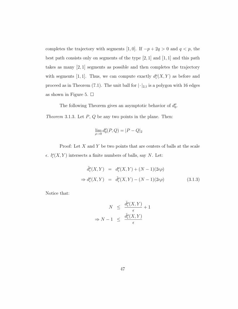
Theorem 3.1.3. Let P , Q be any two points in the plane. Then:

limρ→0

dρ0(P, Q) = |P −Q|2

Proof: Let X and Y be two points that are centers of balls at the scale

ε. lρε (X, Y ) intersects a finite numbers of balls, say N . Let:

dρε (X, Y ) = dρ

ε (X, Y ) + (N − 1)(2ερ)

⇒ dρε (X, Y ) = dρ

ε (X, Y )− (N − 1)(2ερ) (3.1.3)

Notice that:

N ≤ dρε(X, Y )

ε+ 1

⇒ N − 1 ≤ dρε(X, Y )

ε

47

(1,0)0

P

0(1/(1-2r),0)

QR

S

00

r

(1/(1-2r),0)(1/(1-2r),0)

goes to 0

Figure 3.2: Unit balls for limiting norms. P = R = ( 1√2−2ρ

, 1√2−2ρ

), Q =

( 1√5−2ρ

, 2√5−2ρ

), S = ( 2√5−2ρ

, 1√5−2ρ

).

48

Hence, using (7.18):

dρε (X, Y ) ≥ dρ

ε (X, Y )− dρε (X, Y )

ε(2ερ)

= dρε (X, Y )(1− 2ρ)

≥ (1− 2ρ)|X − Y |2 (3.1.4)

Let P ′ and Q′ be the closest points to P and Q respectively, at the scale ε, in

such a way that both P ′ and Q′ are centers of balls. We have that:

dρε (P

′, Q′)− 2ε ≤ dρε(P, Q) ≤ |P −Q|2

Using (7.19), we have:

(1− 2ρ)|P ′ −Q′|2 − 2ε ≤ dρε (P, Q) ≤ |P −Q|2

Using the triangle inequality we have:

(1− 2ρ)(|P −Q|2 − 2ε)− 2ε ≤ dρε (P, Q) ≤ |P −Q|2

⇒ (1− 2ρ)(1− 2ε

|P −Q|2 )− 2ε

|P −Q|2 ≤ dρε(P, Q)

|P −Q|2 ≤ 1

Now letting ε → 0 we have:

1− 2ρ ≤ dρ0(P, Q)

|P −Q|2 ≤ 1

This implies:

limρ→0

dρ0(P, Q) = |P −Q|2

49

Figure 5 shows the unit balls of the effective norms for the cases 2−√22

<

ρ < 0.5, 1+√

2−√52

< ρ ≤ 2−√22

and 1+√

5−√102

< ρ ≤ 1+√

2−√52

. Also, as ρ → 0,

the effective norms converge to the Euclidean norm. Our results suggest that

as ρ gets smaller the behavior of the unit ball changes, though it is always

polygonal with more and mores edges, until it becomes a circle in the limit.

3.2 Connection with Effective Hamiltonians

The theory of homogenization studies the asymptotic behaviour of a

family of partial differential equations, which oscillate with small period size

ε > 0. In this section we want to start exploring the connection between the

results proven in the previous section and the theory of homogenization of

Hamilton-Jacobi equations.

Consider, for each ε, the solution uε to the following problem:

H(Duε,x

ε) = 0 in Ω

uε = 0 on ∂Ω (3.2.5)

where H : Rn × Ω → R satisfies, among others, the following properties:

• H(p, x) is periodic in the x variable.

• H(p, x) is convex in the p variable.

• H is uniformly continuous in the x variable.

• lim|p|→∞ H(p, x) = ∞

50

and Ω is an open set. It can be proven, see for instance [15], that the sequence

of solutions uε has a subsequence that converges uniformly to a Lipschitz

function u. Moreover, u satisfies the following PDE:

H(Du) = 0 in Ω

u = 0 on ∂Ω

where H : Rn → R is defined as follows: For each p ∈ Rn, H(p) is the unique

number for which the PDE:

H(p + Dyv, y) = H(p) in Rn

v is [0, 1]n − periodic (3.2.6)

has a Lipschitz viscosity solution.

The function H is called the effective Hamiltonian and a very interesting

question is to study structure of H and to find explicit formulas for it. This is

still a largely open problem. In [14], Evans gives some partial results in this

direction. See also [12].

In the previous section we proved some results concerning the homog-

enization for the case n = 2. We want to recast those results in the context

of homogenization for Hamilton-Jacobi equations. Even though the results of

the previous section were proven for n = 2, let us define the following function:

uε(x) = dρε (0, x), x ∈ Rn (3.2.7)

We would like to find the Hamilton-Jacobi equation that the previous function

solves. Because of the nature of our domain (we have inclusions and inside of

51

these inclusions the area is neglected), we see that we need to find the PDE

that uε solves outside the inclusions together with the condition the uε satisfies

on the boundary of the inclusions. In the following exposition, let ε = 1 and

fix ρ. Define de function:

v(x) = dρ1(x, 0), x ∈ Rn (3.2.8)

That is, v(x) is the smallest distance from x to the origin at the scale ε = 1.

Recall our notation O = Rn\Inclusions; that is, O is the open set outside

the inclusions. Le H denote the union of all inclusions. Therefore, O = Rn\H .

Notice that our function v is constant on each inclusion I and denote by v(I)

the value of v at any point of the inclusion I. We claim that v satisfies the

following properties:

• |Dv| = 1 in O (in the viscosity sense)

• v is constant on each inclusion I

• v(0) = 0

• ∂v∂ν

(xI) = −1 for some xI ∈ ∂I

Remark 3.2.1. We assume that the the origin is the center of an inclusion

(closed ball).

Since we are measuring the lenght of a curve by neglecting the parts inside

the inclusions, it follows that v is constant on each inclusion I and it is also

clear that v(0) = 0. We will prove now formally that, given any inclusion I

52

there exits a direccion ν an a point xI on ∂I such that ∂v∂ν

(xI) = −1. Take

an inclusion I and let x ∈ ∂I. Let Iε be a neighborhood of I; that is, Iε =

z|d(z, I) < ε. We have that, if ε is small enough:

v(x) = infy∈∂Iε

(d(y, ∂I) + v(y)) (3.2.9)

For each y ∈ ∂I, let ν(y) denote the outward unit normal vector at y. From

3.2.9, if follows that:

0 = infy∈∂Iε

(d(y, ∂I) + v(y)− v(x))

Let y ∈ ∂I denote the point where |y − y| is minimum. Using the fact that

v(y) = v(x) and |y − y| = ε we have:

0 = infy∈∂Iε

(ε + v(y)− v(y))

0 = infy∈∂I

(ε + v(y)− v(y))

0 = infy∈∂I

(1 +v(y + εν(y))− v(y)

ε)

Letting ε → 0 we have 0 = inf∂I(1 + ∂v∂ν

(y)). If this infimum is reached at

xI ∈ ∂I, if follows that ∂v∂ν

(xI) = −1. That is, in at least one point of ∂I,

the graph of v was “growing” just before reaching the constant value v(I)

at that point. We will prove now to that our function v solves the eikonal

equation |Dv| = 1 in the viscosity sense outside the inclusions. Refer to [3]

for the definition an properties of viscosity solutions. We prove first that v is a

viscosity subsolution of |Du| = 1. Let ϕ be a C1 function such that v− ϕ has

a local maximum at the point x0 ∈ O. We need to prove that |Dϕ(x0)| ≤ 1.

53

Since v−ϕ has a local maximum at x0 it follows v(x)− v(x0) ≤ ϕ(x)−ϕ(x0),

for all x in a neighborhood of x0. We can write a point x in B(x0, h) (for h

small enough) as x0 + hz for some z satisfying |z| = 1. We have:

v(x0 + hz)− v(x0) ≤ ϕ(x0 + hz)− ϕ(x0)

=

∫ h

0

d

dsϕ(x0 + sz)

=

∫ h

0

Dϕ(x0 + sz) · zds

≤∫ h

0

Dϕ(x0) · zds + Ch2

for all |z| = 1. If we chose z0 = − Dϕ(x0)|Dϕ(x0)| we have:

v(x0 + hz0)− v(x0) ≤ −∫ h

0

|Dϕ(x0)|ds + Ch2

= −h|Dϕ(x0)|+ Ch2 (3.2.10)

We now use the fact that v is a Lipchitz function and from 3.2.10 we obtain:

h|Dϕ(x0) ≤ v(x0)− v(x0 + hz0) + Ch2

≤ |hz0|+ Ch2

And hence:

|Dϕ(x0)| ≤ 1 + Ch

By letting h → 0 we conclude |Dϕ(x0)| ≤ 1. We prove now that v is a

supersolution. Let ϕ be a C1 function such that v − ϕ has a local minimum

at the point x0 ∈ O. We need to prove that |Dϕ(x0)| ≥ 1. Since v − ϕ has

54

a local minimum at x0 it follows v(x) − v(x0) ≥ ϕ(x) − ϕ(x0), for all x in a

neighborhood of x0. As before, we write a point x in B(x0, h) as x0 + hz for

some z satisfying |z| = 1. We have:

v(x0 + hz)− v(x0) ≥ ϕ(x0 + hz)− ϕ(x0)

=

∫ h

0

d

dsϕ(x0 + sz)

=

∫ h

0

Dϕ(x0 + sz) · zds

≥∫ h

0

Dϕ(x0) · zds − Ch2

≥ −h|Dϕ(x0)| − Ch2 (3.2.11)

for all |z| = 1. Since v(x0) = inf |z|=1h + v(x0 + hz), there exists a point z0

such that v(x0 + hz0) + h ≤ v(x0) + h2 and thus v(x0)− v(x0 + hz0) ≥ h− h2.

Using this and 3.2.11 we obtain:

h|Dϕ(x0) ≥ v(x0)− v(x0 + hz0)− Ch2

≥ h− h2 − Ch2

⇒

|Dϕ(x0) ≥ 1− h− Ch

and letting h → 0 we obtain |Dϕ(x0)| ≥ 1. Consider now the following

Hamilton-Jacobi equation:

|Du| = 1 in O

u = constant on each inclusion I

u(0) = 0 (3.2.12)

55

We have proved that v is a viscosity solution of 3.2.12. We make the following

definition:

Definition 3.2.1. We say that u is a maximal solution of the previous equation

if u(x) ≥ w(x), for any w solution of the problem and any x ∈ Rn.

The ecuacion 3.2.12 could have more than one viscosity solution. How-

ever, we will see that v is the unique maximal solution. That is, any other

solution u satisfies u(x) ≤ v(x). We have the following comparison principle.

Theorem 3.2.1. v is the unique maximal viscosity solution of 3.2.12. That is,

if u solves 3.2.12 in the viscosity sense we have u ≤ v.

Proof: Assume that u a solution for 3.2.12. Consider first the case u

is bounded. Let 0 < θ < 1 and define the function uθ = θu. If we prove that

uθ ≤ v for any 0 < θ < 1, then by letting θ → 1 we obtain u ≤ v. It can

be proven that the function uθ solves the equation |Duθ| = θ in the viscosity

sense. To prove uθ ≤ v we proceed by contradiction. Assume that uθ − v is

positive at some point. Since lim|x|→∞ v = ∞ it follows that uθ−v in negative

outside a large ball BR and therefore uθ−v attains a positive maximun M > 0

inside BR. We claim that all the points where uθ − v attains its maximum

M are in the open set O. To see this suppose that (uθ − v)(x0) = M and

x0 ∈ ∂I for some inclusion I. We proved above that there exists x ∈ ∂I

so that ∂v∂ν

(x) = −1. Since both uθ and v are contant on I it follows that

(uθ−v)(x) = M . We have (uθ−v)(x) ≤ (uθ−v)(x) = M for all x ∈ Rn. If we

denote v = v + M , we have (uθ − v)(x) ≤ 0 for all x ∈ Rn and uθ(x) = v(x).

56

This tells that that graph of uθ is below the graph of v. On the other hand,

since |Duθ| = θ and ∂v∂ν

(x) = −1, it follows that in the direction ν, the graph of

v is strictly below that the graph of uθ which gives a contraction. We conclude

that uθ − v can not attain a maximun at a point on ∂O. Define the function:

Φε(x, y) = uθ(x)− v(y)− 1

ε|x− y|2 (3.2.13)

and let x0 ∈ O be such that (uθ − v)(x0) = M . Since Φε(x0, x0) > 0 and

Φε(x, y) is negative outside a large ball BR×BR we have that Φε(x, y) attains

a positive maximum at a point (xε, yε) ∈ BR × BR. The sequence (xε, yε)has a convergent subsequence (denoted again by (xε, yε)). Let (x, y) =

limε→0(xε, yε). We have:

M = Φε(x0, x0) ≤ Φε(xε, xε)

= uθ(xε)− v(yε)− 1

ε|xε − yε|2 (3.2.14)

≤ uθ(xε)− v(yε)

Since uθ and v are Lipchitz continuos, by letting ε → 0 we obtain:

M ≤ uθ(x)− v(y) (3.2.15)

From 3.2.14 and 3.2.15 we obtain:

1

ε|xε − yε|2 + M ≤ uθ(xε)− v(yε)

≤ uθ(xε)− v(xε) + v(xε)− v(yε)

≤ M + |xε − yε|

57

From this if follows that if xε 6= yε then |xε − yε| ≤ ε. Therefore |x − y| ≤|x − xε| + |xε − yε + |yε − y| ≤ |x − xε| + ε + |yε − y| and by letting ε → 0 it

follows that |x−y| = 0; that is, x = y. From 3.2.15 we have uθ(x)−v(x) = M

and hence x ∈ O. Thus, for ε small enough we have xε ∈ O and yε ∈ O. We

have:

uθ(x)− v(y)− 1

ε|x− y|2 ≤ uθ(xε)− v(yε)− 1

ε|xε − yε|2

for all x, y ∈ Rn. If we fix y = yε we have:

uθ(x)− (v(yε) +1

ε|x− yε|2) ≤ uθ(xε)− (v(yε) +

1

ε|xε − yε|2)

and thus, x → uθ(x)− (v(yε) + 1ε|x− yε|2) has a local maximum at the point

xε. Since |Duθ| ≤ θ we have:

|2ε(xε − yε)| ≤ θ (3.2.16)

Multiplying 3.2.16 by -1 and fixing x = xε we have:

v(y)− (uθ(xε)− 1

ε|xε − y|2) ≥ v(yε)− (uθ(xε)− 1

ε|xε − yε|2)

and thus y → v(y)− (uθ(xε) − 1ε|xε − y|2) has a local minimum at yε. Since

|Dv| ≥ 1 in the viscosity sense we have:

|2ε(xε − yε)| ≥ 1 (3.2.17)

which contradicts 3.2.16. From this contradiction we conclude that uθ ≤ v.

To consider the case u is not bounded, we can use an standard argument

that consists in composing the function u with a suitable function Ψ so that

58

u := Ψ(u) is bounded and |Du| ≤ θ in the viscosity sense. We now give

an sketch of this procedure. Let Ψn : R → R be a C1 function such that

Ψn(r) = θr if |r| ≤ n, Ψn(r) = 0 outside a large ball, |Ψ′n(r)| ≤ θ and

Ψn(r) → r pointwise. Define the function un = Ψn(u). It can be proven that

|Dun| ≤ θ in the viscosity sense and since un is bounded we are in the previous

case and we can conclude un ≤ v. Finally, by letting n →∞ we obtain u ≤ v.

We want to perform now the homogenization of the Hamilton-Jacobi equation

3.2.12. At the scale ε, our domain is the open set εO and the inclusions now

are closed balls or radius ερ. Recall the definition of uε in 3.2.7. We have fixed

the radius ρ and we are interested in the behaviour of the solutions uε of the

Hamilton-Jacobi equation:

|Du| = 1 in Oε

u = constant on each inclusion εI

u(0) = 0

Using standard theory for viscosity solutions we can prove that the sequence

uε has a subsequence that converges uniformly to a function u. In the previous

section we have found explicit formulas for u, at least for some values of ρ and

n = 2. In fact, u(x) = |x|1, |x|1,1 or |x|2,1 depending on the value of ρ (See

previous section). Since we have a formula for u, this suggest that we should be

able to give a formula for the corresponding effective Hamiltonian. However,

we need first to formulate the cell problem (in analogy to 3.2.6) corresponding

to our problem.

59

It would be interesting to be able to find an explicit formula for the

effective Hamiltonian corresponding to this problem because there are few

examples where this can be done. In fact, another interesting project would

be to compute it numerically.

60

Chapter 4

An algorithm to compute weighted minimal

surfaces in 2 and 3 dimensions.

4.1 Preliminaries

In Chapter 2 we constructed periodic surfaces that always stay at a

bounded distance from a given plane, and in this thesis we give an algorithm

for computing these minimal surfaces. The algorithm involves h-adaptive fi-

nite element approximations of the linear convection-diffusion equation. The

latter equation has been shown to linearize the governing nonlinear PDE for

evolution by weighted mean curvature.

The evolution of hypersurfaces Rn according to their mean curvature

has been investigated thoroughly in the literature. There are many results in

this area using parametric methods of differential geometry (See [20], [19],

[23]), and also in the setting of varifold theory from geometric measure theory

(See [6]).

However, a completely different approach was given by Osher and

Sethian in [27]. Their approach, recast slightly, is as follows. Given the

initial hypersurface Γ0, select some continuous function g so that:

Γ0 = x ∈ Rn : g(x) = 0

61

Then, the PDE:

ut = |Du|div(Du

|Du|) in Rn × [0,∞),

u = g on Rn × t = 0 (4.1.1)

evolves the level sets of u according to their mean curvature.

Despite the conciseness of the above formulation, solving this equation

numerically is computationally expensive due to the presence of the nonlinear

elliptic term. Standard methods of solution for equations of this type include

direct methods (Newton iterations), and indirect methods (nonlinear conjugate

gradient). However, these algorithms are computationaly expensive due to

the large number of iterations that are typically needed for convergence. It

is desirable to have an algorithm that is relatively simple to implement and

inexpensive to compute, so that the cost per time step is low. In such a

case many time steps and long-time simulations can be carried out relatively

quickly.

Bence, Merriman and Osher proposed in [25] a numerical algorithm

for computing mean curvature flow using the heat equation and reinitializing

after short time steps. This algorithm is a quasi-linearization of the PDE 4.1.1.

The surface Γ0 is evolved in the following way: let C0 be an open bounded set

with boundary Γ0. Consider the PDE:

ut −∆u = 0 in Rn × (0,∞)

u = ϕC0 on Rn × t = 0 (4.1.2)

62

where ϕC0 is the characteristic function of C0.

The algorithm involves fixing a time step t > 0, defining the new set:

Ct = x ∈ Rn : u(x, t) ≥ 1

2 (4.1.3)

and solving 4.1.2 again but replacing C0 by Ct. In [25] heuristics are given

to show that the evolution of C0 in to Ct aproximates for small times the

mean curvature motion of the boundary Γ0 of C0. Then by repeating this

procedure, i.e. solving the heat equation and reinitializing after a short time,

we approximate mean curvature flow. This is valid even for large times. The

algorithm only involves the heat equation, which is easy to implement numer-

ically and very inexpensive to compute. This allows for long-time simulations

with thousands of time steps, with minimal computational cost.

Proofs of the convergence of this algorithm can be found in Evans [15],

Barles-Georgelin [4].

4.2 The Algorithm

Chapter 2 contains the theoretical results concerning the construction

of our weighted minimal surfaces, and these will be summarized next. Given

ω ∈ Qn, N ∈ Z, M ∈ R, with M, N > 0 we define:

S1 = x ∈ Rn : x · ω ≤ 0

S2 = x ∈ Rn : x · ω ≤ M

63

We refer to Π1 = x ∈ Rn : x · ω = 0 and Π2 = x ∈ Rn : x · ω = Mas the parallel plane restrictions. We minimize area outside the inclusions in

the following class of periodic sets:

AS1,S2 = E : E is a closed Cacciopoli set, S1 ⊂ E ⊂ S2, TNkE =

E, ∀k ∈ Zn with ω · k = 0

Since the sets in AS1,S2 are periodic, we minimize the area outside the

inclusions in an open parallelogram P , representing one period (see figure 2.1

in chapter 2). By applying the standard argument in the calculus of variations

we prove the existence of minimizers.

We now describe an algorithm to compute these minimizers, in the

case of a heterogeneous domain. In our problem the area is measured by

putting a weight of 0 inside the inclusions and a weight of 1 outside the inclu-

sions. In order to treat the discontinuity of the weight in the computations,

we approximate the original minimizer by ε-minimizers corresponding to the

ε-problem (See end of Chapter 2). For the ε-problem, the discontinuous weight

is smoothed using the function ε ≤ w ≤ 1 , with ε << 1, where w has value

ε inside the inclusions and increases smoothly to 1 in a very narrow neigbor-

hood of the inclusion. Since w is smooth, the existence of minimizes for the

ε-problem is contained in [10] and we proved in Chapter 2 that the area of

the ε-minimizers outside the inclusions converges to the area of the true min-

imizer. The minimizers we have constructed are boundary of sets, so they are

not the graph of a function. However, we have regularity for these minimizers

64

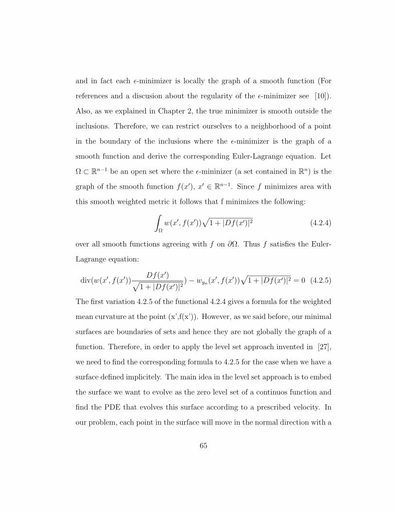
and in fact each ε-minimizer is locally the graph of a smooth function (For

references and a discusion about the regularity of the ε-minimizer see [10]).

Also, as we explained in Chapter 2, the true minimizer is smooth outside the

inclusions. Therefore, we can restrict ourselves to a neighborhood of a point

in the boundary of the inclusions where the ε-minimizer is the graph of a

smooth function and derive the corresponding Euler-Lagrange equation. Let

Ω ⊂ Rn−1 be an open set where the ε-mininizer (a set contained in Rn) is the

graph of the smooth function f(x′), x′ ∈ Rn−1. Since f minimizes area with

this smooth weighted metric it follows that f minimizes the following:∫Ω

w(x′, f(x′))√

1 + |Df(x′)|2 (4.2.4)

over all smooth functions agreeing with f on ∂Ω. Thus f satisfies the Euler-

Lagrange equation:

div(w(x′, f(x′))Df(x′)√

1 + |Df(x′)|2 )− wyn(x′, f(x′))√

1 + |Df(x′)|2 = 0 (4.2.5)

The first variation 4.2.5 of the functional 4.2.4 gives a formula for the weighted

mean curvature at the point (x’,f(x’)). However, as we said before, our minimal

surfaces are boundaries of sets and hence they are not globally the graph of a

function. Therefore, in order to apply the level set approach invented in [27],

we need to find the corresponding formula to 4.2.5 for the case when we have a

surface defined implicitely. The main idea in the level set approach is to embed

the surface we want to evolve as the zero level set of a continuos function and

find the PDE that evolves this surface according to a prescribed velocity. In

our problem, each point in the surface will move in the normal direction with a

65

velocity −Hw, where Hw(x) is the weighted mean curvature at each point x of

the surface. More precisely, suppose we have Γ0 = x ∈ Rn : g(x) = 0, where

g is a smooth function. Notice that by doing this, we have added one more

dimension to the problem. We want to evolve Γ0 according to its weighted

mean curvature. Suppose that at each time t ≥ 0, the evolved hypersurface

is given implicitely by the equation u(x, t) = 0. Then u(x, 0) = g(x). Let

x ∈ Rn and let α(s), α(t) = x, be the trajectory of x under this evolution.

We have that u(α(s), s) = 0 for all s. Differentiating with respect to s gives

that ut(α(s), s)+Du(α(s), s) ·α′(s) = 0; that is, ut(x, t) +Du(x, t) ·α′(t) = 0.

However,

α′(t) = −Hw(x)Du

|Du| (4.2.6)

Since Du|Du| is the exterior unit normal vector at x, 4.2.6 says we are evolving the

surface in the normal direction with velocity −Hw(x). Since we are evolving

the level sets of u and we know that locally these level sets are the graph of

a function, we can use 4.2.5 to prove (after a somewhat lenghty computation)

that:

Hw(x) = div(w(x)Du

|Du|) (4.2.7)

Notice that the second term in 4.2.5 does not appear in Hw. Thus, we obtain:

ut(x, t) = Du ·Hw(x)Du

|Du|= |Du|Hw(x)

= |Du|div(w(x)Du

|Du|)

66

Then, the PDE that evolves Γ0 according to its weighted mean curvature is:

ut(x, t) = |Du|div(w(x)Du

|Du|)

u(x, 0) = g(x) (4.2.8)

We consider a linearization of 4.2.8 analogous to the linearization of equation

4.1.1 by 4.1.2. That is, we want to find a BMO ( [25]) version for the equation

4.2.8. This is in fact possible and the equation:

ut(x, t) = div(w(x)Du) +1

2Dw ·Du

u(x, 0) = g(x) (4.2.9)

when reinitialized after small times, converges to equation 4.2.8. More specif-

ically, if we let Ω0 be an open set such that ∂Ω0 = Γ0, then the following

scheme:

• u∆t(x, 0) = ϕΩ0 − ϕΩc0

• Solve:

vt = div(w(x)Dv) + 12Dw ·Dv, in Rn × (0, ∆t]

v(x, 0) = u∆t(x, (n− 1)∆t)

• u∆t(x, n∆t) = 1, if v(x, ∆t) > 0

u∆t(x, n∆t) = −1, if v(x, ∆t) ≤ 0

converges, as ∆t → 0, to motion by weigthed mean curvature. Note that this

algorithm contains not only the standard diffusion term div(w(x)Du), but

also the convective term 12Dw ·Du.

67

A proof of this can be found in [24]. Our problem is a particular case

of a more general situation considered in [24].

4.3 Numerical implementation

We now implement the BMO algorithm corresponding to motion by

weigthed mean curvature. We solve the equation 4.2.9 in the domain P , which

is the parallelogram that represents one period (see Figure 4.1), using Dirichlet

boundary conditions 1 and 0 on the bottom and the top of P respectively. Our

initial condition is the characteristic function of the set below a parallel plane

to the restrictions Π1 and Π2 (set C in Figure 4.1). We solve the equation

4.2.9 for a small time and then reinitialize, in the same way as for equation

4.1.2. The algorithm can be summarized as follows:

1. Let u0 = ϕC

2. Solve:

ut(x, t) = div(w(x)Du(x, t)) +1

2Dw ·Du

u(x, 0) = u0

3. Reinitialize at t = Tchop:

if u(xi) ≥ 0.5 ⇒ set u0(xi) = 1 else set u0(xi) = 0

4. Repeat step 2

The location of the front is given by the level set u = 12

68

Initial Condition (set C)

Dirichlet condition =1

Dirichlet condition = 0

Periodic boundary condition

Figure 4.1: Diagram showing the domain with inclusions where we are solvingthe equation 4.2.9

69

The algorithm has been implemented in two and three dimensions. The

spatial discretization was accomplished using the Fortran 90 codes 2Dhp90

and 3Dhp90, both from the Texas Institute for Computational and Applied

Mathematics. These codes solve the the equation Dj(aijui) = 0 in two and

three dimensions, respectively, with built-in capability for local adaptivity.

Local adaptivity is very important for resolving the discontinuities along the

interfaces of the inclusions, as well as for accurately representing inclusions

with complex shapes. The time discretization was a simple backward Euler

scheme for the time derivative, and carrying the convective term to the right

hand side. The main modifications to the codes include:

1. Implementation of the time dependence.

2. Reinitialization after the chopping time Tchop.

3. Periodic boundary conditions and local refinements of the mesh around

the inclusions.

4. Implementation of the convective term 12Du ·Dw.

4.4 Results

We present results for dimensions 2 and 3 (see figures at the end).

Since the algorithm can not differentiate by itself a local minimizer from a

global minimizer, we need to consider the posibility of the algorithm converging

to a local minimizer; that is, a minimizer that satisfies zero weighted mean

70

curvature but that is not a global minimizer. However, this difficulty can

be solved by stoping the chopping process and diffusing for a time until the

surface continues its evolution. This is the well known tecnique of annealing

used in numerical analysis to pertubate a local minimizer while looking for a

global one.

The algorithm evolves the initial condition, which is always given by

the plane ω · x = b where ω is the slope of the parallel plane restrictions. As

you can see from the pictures, the initial condition is not a global minimizer.

There are four diferent parameters that affect the evolution of the surface: ∆t

denotes the time step, mod denotes the number of iterations between any two

reinitializations, iter denotes the total number of iterations we perform and b

tells how far from the lower constraint we want to place our initial condition.

We have found experimentally that the value of mod is important in order to

get a good result. In general, mod depends on the number of iterations and

the time step but a value between 5 and 8 works well. If mod is too small, it is

difficult for the surface to evolve and it could not even evolve at all (compare

for example Figures 4.8 and 4.9). On the the other hand, if mod is too large,

then we are practically only diffusing and the resulting surface is a very bad

approximation of a surface that must satisfies zero mean curvature outside and

inside the inclusions (compare Figures 4.3 and 4.2). Notice that in Figure 4.2,

we get a much better approximation of a surface that has zero mean curvature

outside the inclusions (for n=2 the minimal surface is composed by pieces of

lines).

71

An interesting question is to determine the role that the convective

term plays in the evolution. Our numerical experiments show that the convec-

tive term acts as an extra force that pushes up the surface near an inclusion.

The examples in Figures 4.5, 4.7 and 4.10 were obtained by computing only

the diffusion term. Compare these Figures with the Figures 4.4, 4.6 and 4.8

respectively. Figure 4.11 was obtained using the same values of the param-

eters as Figure 4.8 with the exception that in Figure 4.11 we split the time

step by 2 and doble the number of iterations, and since both results are the

same we can conclude that the algorithm converges in the time discretization.

Also, an advantage of our algorithm is that stability is not an issue, since the

reinitializations takes out any growing inestability.

72

Figure 4.2: A 2-Dimensional h-adaptive finite element simulation of motion byweighted mean curvature. The initial surface was a straight line parallel andclose to the bottom of the domain. The grid in the figure is the mesh used tosolve the PDE. The parameters are: mod=6, ∆t = 0.01, iter=100, b=0.1

73

Figure 4.3: A 2-Dimensional h-adaptive finite element simulation of motion byweighted mean curvature. The initial surface was a straight line parallel andclose to the bottom of the domain. The grid in the figure is the mesh used tosolve the PDE. The parameters are mod = 12, ∆t = 0.01, iter=100, b=0.1

74

Figure 4.4: A 2-Dimensional h-adaptive finite element simulation of motionby weighted mean curvature. The initial surface was a straight line paralleland close to the bottom of the domain. The grid in the figure is the mesh usedto solve the PDE. Compare this result with the next one, which only containsthe diffusion term. Compare also with Figure 4.2, in which we performed 100iterations instead of 25. The parameters are: mod=6, ∆t = 0.01, iter=25,b=0.1

75

Figure 4.5: A 2-Dimensional h-adaptive finite element simulation of motionby weighted mean curvature. The initial surface was a straight line paralleland close to the bottom of the domain. The grid in the figure is the meshused to solve the PDE. This example contains only the diffusion term. Theparameters are: mod=6, ∆t = 0.01, iter=25, b=0.1

76

Figure 4.6: A 2-Dimensional h-adaptive finite element simulation of motion byweighted mean curvature. The initial surface was a straight line parallel andclose to the bottom of the domain. The grid in the figure is the mesh used tosolve the PDE. Note the refinement of the mesh around the inclusions. Theparameters are: mod=8, ∆t = 0.01, iter=100, b=0.05

77

Figure 4.7: A 2-Dimensional h-adaptive finite element simulation of motion byweighted mean curvature. The initial surface was a straight line parallel andclose to the bottom of the domain. This simulation contains only the diffusionterm. The grid in the figure is the mesh used to solve the PDE. Note therefinement of the mesh around the inclusions. The parameters are: mod=8,∆t = 0.01, iter=100, b=0.05

78

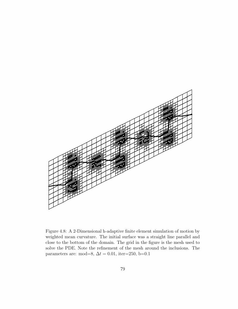
Figure 4.8: A 2-Dimensional h-adaptive finite element simulation of motion byweighted mean curvature. The initial surface was a straight line parallel andclose to the bottom of the domain. The grid in the figure is the mesh used tosolve the PDE. Note the refinement of the mesh around the inclusions. Theparameters are: mod=8, ∆t = 0.01, iter=250, b=0.1

79

Figure 4.9: A 2-Dimensional h-adaptive finite element simulation of motion byweighted mean curvature. The initial surface was a straight line parallel andclose to the bottom of the domain. The grid in the figure is the mesh used tosolve the PDE. Note the refinement of the mesh around the inclusions. Theparameters are: mod=4, ∆t = 0.01, iter=250, b=0.1

80

Figure 4.10: A 2-Dimensional h-adaptive finite element simulation of motionby weighted mean curvature. The initial surface was a straight line paralleland close to the bottom of the domain. This simulation contains only thediffusion term. The grid in the figure is the mesh used to solve the PDE.Note the refinement of the mesh around the inclusions. The parameters are:mod=8, ∆t = 0.01, iter=250, b=0.1

81

Figure 4.11: A 2-Dimensional h-adaptive finite element simulation of motionby weighted mean curvature. The initial surface was a straight line paralleland close to the bottom of the domain. The grid in the figure is the mesh usedto solve the PDE. Note the refinement of the mesh around the inclusions. Theparameters are: mod=16, ∆t = 0.005, iter=500, b=0.1

82

X

Z

Y

X

Z

Y

X

Z

YX

Z

Y

Figure 4.12: A 3-Dimensional h-adaptive finite element simulation of motionby weighted mean curvature. The initial surface was a plane parallel and closeto the bottom of the domain. We are showing two different views of the sameevolution. For clarity we only show the surface and the elements of the meshthat form the inclusions. The parameters are: mod=6, ∆t = 0.01, iter=350(we start sharpening after the first 100 iterations), b=0.02

83

Bibliography

[1] F. J. Almgren, Jr. Existence and regularity almost everywhere of so-

lutions to elliptic variational problems with constraints. Mem. Amer.

Math. Soc., 4(165):viii+199, 1976.

[2] F. Auer. Minimale hyperflachen in riemannsche n-torus. Albert-Ludwigs

Univ. thesis, 1997.

[3] Martino Bardi and Italo Capuzzo-Dolcetta. Optimal control and viscosity

solutions of Hamilton-Jacobi-Bellman equations. Birkhauser Boston Inc.,

Boston, MA, 1997. With appendices by Maurizio Falcone and Pierpaolo

Soravia.

[4] Guy Barles and Christine Georgelin. A simple proof of convergence for an

approximation scheme for computing motions by mean curvature. SIAM

J. Numer. Anal., 32(2):484–500, 1995.

[5] Guy Barles and Panagiotis E. Souganidis. A new approach to front

propagation problems: theory and applications. Arch. Rational Mech.

Anal., 141(3):237–296, 1998.

[6] Kenneth A. Brakke. The motion of a surface by its mean curvature.

Princeton University Press, Princeton, N.J., 1978.

84

[7] L. A. Caffarelli. A note on nonlinear homogenization. Comm. Pure

Appl. Math., 52(7):829–838, 1999.

[8] Luis A. Caffarelli and Antonio Cordoba. An elementary regularity theory

of minimal surfaces. Differential Integral Equations, 6(1):1–13, 1993.

[9] Luis A. Caffarelli and Antonio Cordoba. Correction: “An elementary

regularity theory of minimal surfaces” [Differential Integral Equations

6 (1993), no. 1, 1–13; MR 94c:49042]. Differential Integral Equations,

8(1):223, 1995.

[10] Luis A. Caffarelli and Rafael de la Llave. Planelike minimizers in periodic

media. Comm. Pure Appl. Math., 54(12):1403–1441, 2001.

[11] M. G. Crandall, L. C. Evans, and P.-L. Lions. Some properties of viscosity

solutions of Hamilton-Jacobi equations. Trans. Amer. Math. Soc.,

282(2):487–502, 1984.

[12] L. C. Evans and D. Gomes. Effective Hamiltonians and averaging for

Hamiltonian dynamics. I. Arch. Ration. Mech. Anal., 157(1):1–33,

2001.

[13] Lawrence C. Evans. The perturbed test function method for viscosity

solutions of nonlinear PDE. Proc. Roy. Soc. Edinburgh Sect. A, 111(3-

4):359–375, 1989.

85

[14] Lawrence C. Evans. Periodic homogenisation of certain fully nonlinear

partial differential equations. Proc. Roy. Soc. Edinburgh Sect. A,

120(3-4):245–265, 1992.

[15] Lawrence C. Evans. Convergence of an algorithm for mean curvature

motion. Indiana Univ. Math. J., 42(2):533–557, 1993.

[16] Lawrence C. Evans and Ronald F. Gariepy. Measure theory and fine

properties of functions. CRC Press, Boca Raton, FL, 1992.

[17] Herbert Federer. Geometric measure theory. Springer-Verlag New

York Inc., New York, 1969. Die Grundlehren der mathematischen Wis-

senschaften, Band 153.

[18] Enrico Giusti. Minimal surfaces and functions of bounded variation.

Birkhauser Verlag, Basel, 1984.

[19] Matthew A. Grayson. The heat equation shrinks embedded plane curves

to round points. J. Differential Geom., 26(2):285–314, 1987.

[20] Matthew A. Grayson. A short note on the evolution of a surface by its

mean curvature. Duke Math. J., 58(3):555–558, 1989.

[21] Michael Gruter. Optimal regularity for codimension one minimal surfaces

with a free boundary. Manuscripta Math., 58(3):295–343, 1987.

[22] G.A. Hedlund. Geodesics on a two-dimensional Riemannian manifold

with periodic coefficients. Ann. of Math., 33:719–739, 1932.

86

[23] Gerhard Huisken. Flow by mean curvature of convex surfaces into

spheres. J. Differential Geom., 20(1):237–266, 1984.

[24] Fabiana Leoni. Convergence of and aproximation scheme for curvature-

dependent motions of sets. SIAM J. Numer. Anal., 39(4):1115–1131,

2001.

[25] Barry Merriman, James K. Bence, and Stanley J. Osher. Motion of

multiple functions: a level set approach. J. Comput. Phys., 112(2):334–

363, 1994.

[26] Jurgen Moser. Minimal solutions of variational problems on a torus.

Ann. Inst. H. Poincare Anal. Non Lineaire, 3(3):229–272, 1986.

[27] Stanley Osher and James A. Sethian. Fronts propagating with curvature-

dependent speed: algorithms based on Hamilton-Jacobi formulations. J.

Comput. Phys., 79(1):12–49, 1988.

[28] Leon Simon. Lectures on geometric measure theory. Australian National

University Centre for Mathematical Analysis, Canberra, 1983.

87

Vita

Monica Torres was born in Irapuato, Gto; Mexico, the daugther of

Raul Torres Gallardo and Laura R. de Torres. She received a Bachelor of Sci-

ence degree in Computer Science from the Instituto Tecnologico y de Estudios

Superiores de Monterrey and a Master of Science degree in pure mathematics

from the Centro de Investigaciones Matematicas. She was enrolled in the Ph.D

program in Mathematics at the University of Texas at Austin in August, 1997.

Permanent address: 2400 Eunice St.Berkeley, CA 94708

This dissertation was typeset with LATEX† by the author.

†LATEX is a document preparation system developed by Leslie Lamport as a specialversion of Donald Knuth’s TEX Program.

88