Copyright

by

Mauricio Santillana

2008

The Dissertation Committee for Mauricio Santillana

certifies that this is the approved version of the following dissertation:

Analysis and Numerical Simulation of the Diffusive Wave

Approximation of the Shallow Water Equations

Committee:

Clint N. Dawson, Supervisor

Mary F. Wheeler

Bjorn Engquist

Irene M. Gamba

Bayani Cardenas

Analysis and Numerical Simulation of the Diffusive Wave

Approximation of the Shallow Water Equations

by

Mauricio Santillana, B.S., M.S.

Dissertation

Presented to the Faculty of the Graduate School of

The University of Texas at Austin

in Partial Fulfillment

of the Requirements

for the Degree of

Doctor of Philosophy

The University of Texas at Austin

August 2008

To my mother Luz Patricia, in memoriam...

Acknowledgments

I would like to thank my advisor, Clint Dawson, for his support and encouragement to

pursue the current investigation. I deeply appreciate his patience and help during difficult

times of my life in my years at UT Austin. I would like to thank my colleague and friend,

Ricardo Alonso, for all the support and interest he showed when I tried to drag him into

studying the DSW equation. He was very patient with me and taught me many concepts

and techniques applied throughout this work.

I would like to thank Irene M. Gamba, for her guidance and support. In fact, it was

Irene who convinced me to pursue my graduate work at UT Austin and she was very kind

to support me throughout all my years at UT, both as an academic advisor and as a friend.

I would also like to thank Dr. Mary F. Wheeler for her support and advise. She represents

an example of leadership and scholarship to me. I would like to thank Dr. Bjorn Engquist

for the eye opening lectures on mathematical modeling and numerical analysis from which

I benefited greatly. I would like to thank Dr. Bayani Cardenas for accepting to become a

member of my committee and reading through my work.

I would like to thank Juan Luis Vazquez for the patient guidance he offered me in

the field of nonlinear diffusion equations and for the many insightful conversations we had

during his visit to UT Austin in the Fall of 2007. I would also like to thank Luis Caffarelli

for having the patience to hear many of the disconnected ideas I presented to him, and giv-

ing me in return meaningful insights about my work. I would also like to thank Rafael de

la Llave for his kind guidance and support throughout all my years at UT, both as a friend

v

and as academic advisor. I would like to thank Dr. Tinsley Oden, for having supported me

during my first years at UT.

I would like to thank many of my fellow ICES graduate students, Ross Heath, Marco

A. Iglesias, Sri Harsha T. , Victor Calo, Konstantine Mardanov, Yuri Bazilevs, Shweta

Bansal, among many others that I might have not mentioned, for their enthusiasm and

support. I would like to thank both Connie Baxter and Lorraine Sanchez for their support

and kind friendship.

I would like to thank the Director of CentroGeo, Dr. Carmen Reyes for all her kind

advise and support. She represents an example of leadership and achievement to me. I

would like to thank CentroGeo for partially supporting my graduate stay at UT.

I would like to thank my beloved wife, Monica Yudron, for her unconditional love,

support, and for the extreme patience she showed to me during the development of this

work. She was very kind to read many of the drafts that lead to the final version of this

work and she offered me extremely meaningful suggestions in numerous occasions.

Finally, I would like to thank my brother Humberto, my father, my mother (to whom

I dedicate this thesis), my sister Maru, my brother Sebastian, Fabiola, Maru and Erik for

their love and support.

Mauricio Santillana

The University of Texas at Austin

August 2008

vi

Analysis and Numerical Simulation of the Diffusive Wave

Approximation of the Shallow Water Equations

Publication No.

Mauricio Santillana, Ph.D.

The University of Texas at Austin, 2008

Supervisor: Clint N. Dawson

In this dissertation, the quantitative and qualitative aspects of modeling shallow water

flow driven mainly by gravitational forces and dominated by shear stress, using an effective

equation often referred to in the literature as the diffusive wave approximation of the shallow

water equations (DSW) are presented. These flow conditions arise for example in overland

flow and water flow in vegetated areas such as wetlands. The DSW equation arises in shallow

water flow models when special assumptions are used to simplify the shallow water equations

and contains as particular cases: the Porous Medium equation and the time evolution of the

p-Laplacian. It has been successfully applied as a suitable model to simulate overland flow

and water flow in vegetated areas such as wetlands; yet, no formal mathematical analysis

has been carried out addressing, for example, conditions for which weak solutions may exist,

and conditions for which a numerical scheme can be successful in approximating them. This

vii

thesis represents a first step in that direction. The outline of the thesis is as follows. First,

a survey of relevant results coming from the studies of doubly nonlinear diffusion equations

that can be applied to the DSW equation when topographic effects are ignored, is presented.

Furthermore, an original proof of existence of weak solutions using constructive techniques

that directly lead to the implementation of numerical algorithms to obtain approximate

solutions is shown. Some regularity results about weak solutions are presented as well.

Second, a numerical approach is proposed as a means to understand some properties of

solutions to the DSW equation, when topographic effects are considered, and conditions for

which the continuous and discontinuous Galerkin methods will succeed in approximating

these weak solutions are established.

viii

Contents

Acknowledgments v

Abstract vii

List of Tables xi

List of Figures xii

Chapter 1 Introduction 1

1.1 Motivation . . . . . . . . . . . . . . . . . . . . . . . . . . . . . . . . . . . . 11.2 Literature review . . . . . . . . . . . . . . . . . . . . . . . . . . . . . . . . . 6

1.2.1 Modeling overland flow . . . . . . . . . . . . . . . . . . . . . . . . . 61.2.2 Doubly nonlinear diffusion equations . . . . . . . . . . . . . . . . . . 91.2.3 Numerical methods for nonlinear parabolic problems . . . . . . . . . 13

1.3 Accomplishments . . . . . . . . . . . . . . . . . . . . . . . . . . . . . . . . . 17

Chapter 2 The DSW Equation and Preliminaries 19

2.1 The initial-boundary value problem . . . . . . . . . . . . . . . . . . . . . . . 192.2 Derivation from the shallow water equations . . . . . . . . . . . . . . . . . . 202.3 Notation . . . . . . . . . . . . . . . . . . . . . . . . . . . . . . . . . . . . . . 242.4 Interpolation theory results. Continuous case . . . . . . . . . . . . . . . . . 252.5 Interpolation theory results. Discontinuous case . . . . . . . . . . . . . . . . 26

Chapter 3 Existence, Regularity and Uniqueness of Weak Solutions 27

3.0.1 The obstacle problem . . . . . . . . . . . . . . . . . . . . . . . . . . 283.0.2 Regularization technique . . . . . . . . . . . . . . . . . . . . . . . . . 293.0.3 Definitions of Weak Solutions . . . . . . . . . . . . . . . . . . . . . . 29

3.1 Existence . . . . . . . . . . . . . . . . . . . . . . . . . . . . . . . . . . . . . 313.2 Regularity . . . . . . . . . . . . . . . . . . . . . . . . . . . . . . . . . . . . . 403.3 Comparison result, uniqueness and nonnegativity . . . . . . . . . . . . . . . 463.4 Open problem: topographic effects . . . . . . . . . . . . . . . . . . . . . . . 50

ix

Chapter 4 A Continuous Galerkin Approach 52

4.1 Preliminaries . . . . . . . . . . . . . . . . . . . . . . . . . . . . . . . . . . . 534.2 Regularized problem . . . . . . . . . . . . . . . . . . . . . . . . . . . . . . . 56

4.2.1 Auxiliary results . . . . . . . . . . . . . . . . . . . . . . . . . . . . . 574.3 The Continuous Galerkin Method . . . . . . . . . . . . . . . . . . . . . . . . 57

4.3.1 The semi-discrete case . . . . . . . . . . . . . . . . . . . . . . . . . . 584.3.2 Existence of the continuous in time Galerkin approximation . . . . . 594.3.3 Continuous in time a priori error estimate . . . . . . . . . . . . . . . 604.3.4 Fully discrete approximation . . . . . . . . . . . . . . . . . . . . . . 65

4.4 Numerical Experiments. 1D . . . . . . . . . . . . . . . . . . . . . . . . . . . 684.4.1 Convergence analysis . . . . . . . . . . . . . . . . . . . . . . . . . . . 694.4.2 Validation: Iwagaki’s experiment . . . . . . . . . . . . . . . . . . . . 744.4.3 Qualitative properties of solutions . . . . . . . . . . . . . . . . . . . 77

Chapter 5 A Discontinuous Galerkin Method 79

5.1 Preliminaries . . . . . . . . . . . . . . . . . . . . . . . . . . . . . . . . . . . 795.2 The Local Discontinuous Galerkin Method . . . . . . . . . . . . . . . . . . . 80

5.2.1 Stability analysis . . . . . . . . . . . . . . . . . . . . . . . . . . . . . 835.2.2 Continuous in time a priori error analysis . . . . . . . . . . . . . . . 85

5.3 Numerical Experiments. 2D . . . . . . . . . . . . . . . . . . . . . . . . . . . 905.3.1 The Dam Break problem . . . . . . . . . . . . . . . . . . . . . . . . 925.3.2 The Dam Break problem with vegetation . . . . . . . . . . . . . . . 97

Chapter 6 Concluding Remarks and Future Work 103

6.1 Future work . . . . . . . . . . . . . . . . . . . . . . . . . . . . . . . . . . . . 105

Appendix A Additional results 106

Bibliography 110

Vita 116

x

List of Tables

4.1 Convergence rates. Barenblatt solutions for α = 5/3 and γ = 1/2. . . . . . . 724.2 Convergence rates. Artificial right hand side with t0 = 9 and tf = 9.1 . . . 73

xi

List of Figures

1.1 Surface elevation diagram . . . . . . . . . . . . . . . . . . . . . . . . . . . . 7

3.1 Plots of φ vs φreg . . . . . . . . . . . . . . . . . . . . . . . . . . . . . . . . 30

4.1 Compactly supported solutions . . . . . . . . . . . . . . . . . . . . . . . . . 704.2 Artificial right hand side . . . . . . . . . . . . . . . . . . . . . . . . . . . . . 744.3 Iwagaki’s depth profile experimental results . . . . . . . . . . . . . . . . . . 754.4 Iwagaki’s hydrograph experimental results . . . . . . . . . . . . . . . . . . . 764.5 Qualitative properties of solutions . . . . . . . . . . . . . . . . . . . . . . . 774.6 Qualitative properties of solutions . . . . . . . . . . . . . . . . . . . . . . . 78

5.1 Dam break simulation. Mesh . . . . . . . . . . . . . . . . . . . . . . . . . . 915.2 Dam break simulation. Times=0, 0.5, and 3.0 seconds . . . . . . . . . . . . 935.3 Dam break simulation. Times=5.0, 7.0, and 9.0 seconds . . . . . . . . . . . 945.4 Dam break simulation. Times=15.0, 39.0, and 61.0 seconds . . . . . . . . . 955.5 Side views, Dam break simulation at different times . . . . . . . . . . . . . 965.6 Dam break simulation with vegetation. Mesh . . . . . . . . . . . . . . . . . 985.7 Dam break simulation with vegetation. Times=0, 1.0, and 3.0 seconds . . . 995.8 Dam break simulation with vegetation. Times=5.0, 7.0, and 9.0 seconds . . 1005.9 Dam break simulation with vegetation. Times=11, 13, and 17 seconds . . . 101

xii

Chapter 1

Introduction

1.1 Motivation

The purpose of this thesis is to study, analytically and numerically, an efective equation

often referred to in the literature as the diffusive wave approximation of the shallow water

system of equations. This equation has been used to simulate overland flow in wetlands

and open channels.

Wetlands are some of the most important ecosystems on earth. Historically, they

have been called swamps, marshes, bogs, fens, or sloughs. Since wetlands provide an abun-

dant supply of water, they are able to host a variety of plant and animal species including

mammals, birds, reptiles, amphibians, and fishes. During the past decades, the increased

degradation of wetlands has been connected to damage to the overall biodiversity of our

planet. Consequently, natural wetlands are increasingly protected and construction of arti-

ficial wetlands is being encouraged.

Of particular interest is the relevant role that wetlands can play during storm surges

and flooding events. Indeed, coastal marshes and swamps act as a buffer zone, for example,

between the Gulf of Mexico and inhabited inland areas in Louisiana, where an estimated

60-75 % of residents live within 50 miles of the coast (1993) and where between 1899 and

1995 over a dozen major hurricanes (class 3-5) have hit1 (with the two most recent hits of

category 5 hurricanes Katrina and Rita in 2005). Wetlands also buffer the tidal increase and

wave intensity of hurricanes, since they act as energy dissipators; they provide natural flood

control by detaining and slowing flood waters, and they help protect areas prone to serious

1Source: USGS National Wetlands Research Center. http://www.lacoast.gov/

1

erosion. Furthermore, hurricane winds subside substantially once they reach the wetland

buffer. Another fact about wetlands that make them an important subject of study is that

due to the high rate of biological activity, wetlands can transform many common pollutants

that occur in waste waters into harmless byproducts or into nutrients that can be used for

biological productivity. Thus, it is clear that understanding the dynamics of the flows in

such environments is essential, in particular for management and designing purposes. In

this work, we intend to provide insight to improve the ways in which we model flow con-

ditions in vegetated areas, such as wetlands, in order to deepen our understanding of such

ecologically rich environments.

Wetlands are frequently transitional areas between uplands (terrestrial systems) and

continuously or deeply flooded (aquatic) systems. They are also found at topographic lows

or in areas with high slopes and low permeability soils such as seepage slopes. Overland

flow is a term used to describe water flow regimes in these environments, where uniform

and fully developed turbulent flow conditions arise since the water flow is driven mainly by

gravitational forces and dominated by shear stress. More precisely, overland flow is a term

that is used mostly to describe the shallow movement of water across land surfaces both

when rainfall has exceeded the infiltration rate of the ground’s surface (Horton Overland

Flow), and when the entire soil column becomes completely saturated and water exfiltrates

at the surface (Dunne Overland Flow). An effective equation that has been used to simulate

these particular water flow regimes is a doubly nonlinear and degenerate diffusion equation

often referred to in the literature as the diffusive wave approximation of the shallow water

equations (DSW). This equation is obtained from the shallow water system of equations, by

approximating the 2-D depth-averaged continuity equations by empirical laws commonly

used in open channel flow theory, such as Manning’s or Chezy’s formulas, and combining

the resulting expression with the free surface boundary condition. Formally speaking, the

DSW equation is given by

∂u

∂t−∇ ·

((u− z)α

cf |∇u|1−γ∇u

)= f

where u(x, y; t) is the free surface water elevation, z(x, y) the bed surface or bathymetry,

u − z the water depth, f(x, y, t) a source/sink, and cf is a friction coefficient. The values

of α and γ correspond to, α = 5/3 and γ = 1/2 for Manning’s formula, and α = 3/2 and

γ = 1/2 for Chezy’s formula.

Diverse numerical schemes have been implemented to approximately solve the DSW

2

equation and have been successfully applied as suitable models to simulate overland flow

and water flow in vegetated areas such as wetlands ([69], [44], [17], [38], [39]); yet, to the

best of our knowledge, no formal mathematical analysis has been carried out in order to

study existence, uniqueness, and regularity of weak solutions to this equation; and as a

consequence, the approximation properties of numerical methods, such as error estimates

between the true solution (if uniqueness holds) and the numerical approximant, rates of

convergence, and so on, have not been developed for this equation.

To motivate more deeply this study, it is important to mention that solving the

DSW equation computationally requires significantly less work than solving the shallow

water system of equations (SWE), see [44]. However, despite the obvious appeal to use the

DSW in lieu of the SWE, analysing the mathematical properties of the DSW equation is not

a simple task. Note that the DSW equation contains as particular cases two complicated

nonlinear diffusion equations: the Porous Medium equation (when z = 0 and γ = 1) and

the p-Laplacian for 1 < p < 2 (when α = 0 and p = γ + 1, this case is not considered in

this work).

In this thesis, we will set up the appropriate initial boundary value problem arising

from the DSW equation. This will be done by combining the knowledge from the modeling

applications of the DSW ([69], [44], [17], [38], [39]) and the knowledge coming from exper-

imental works (such as [61]) where the parameters α and γ are considered to be flexible

(generally in the ranges α > 1 and 0 < γ ≤ 1) as a way to account for more general cir-

cumstances when flow changes back and forth between turbulent and laminar conditions in

vegetated regions. We also carry out an investigation of the mathematical properties of the

DSW equation, addressing the mathematical issues discussed in the previous paragraphs.

The DSW equation can be characterized as a doubly nonlinear parabolic equation

and gives rise to the initial boundary value problem (2.1) stated in Chapter 2. Its doubly

nonlinear nature comes from the fact that the nonlinear behavior appears inside the diver-

gence term as a product of two nonlinearities involving u and ∇u, namely (u − z)α and

∇u/|∇u|1−γ . Furthermore, when rewriting it as (for cf ≡ 1):

∂u

∂t−∇ · (a(u,∇u) ∇u) = f with a(u,∇u) =

(u− z)α

|∇u|1−γ, (1.1)

where a is the diffusion coefficient, one can be more specific and characterize it as a doubly

nonlinear and degenerate-singular equation. This is the case since a→ 0 when (u− z) → 0

3

and a → ∞ when ∇u → 0 for the given choice of 0 < γ ≤ 1, and 1 < α < 2. Impor-

tant works addressing existence, uniqueness and regularity of solutions to doubly nonlinear

parabolic equations related to the DSW equations include: [56], [41], [6], [45], and [35].

These works will provide the starting point of this thesis.

Previous work aimed to analyse approximate solutions to nonlinear diffusion equa-

tions using the Galerkin finite element method, such as the work of Wheeler [67] and Douglas

and Dupont [32], deal with equations with nonlinear diffusion coefficients that only depend

on the function u itself and not on ∇u, i.e. diffusion coefficients of the form a = a(u). The

analysis carried out in such cases requires roughly two assumptions,

0 < µ ≤ a(u) ≤M, and |a′(u)| ≤ B for u ∈ R (1.2)

so that a is uniformly Lipschitz with respect to u and bounded below by a small constant

µ. These assumptions ensure in particular, that one can construct a weak formulation such

that, for some Sobolev space V , one has two fundamental conditions:

µ‖u‖2V ≤ (a(u)∇u,∇u) and (a(u)∇u,∇w) ≤M‖u‖V ‖w‖V for u,w ∈ V, (1.3)

where (·, ·) represents the appropriate duality pairing. The doubly nonlinear nature of the

DSW equation poses new challenges that come from the possible degeneracy of the diffusion

coefficient a in (1.1) when (u − z) = 0 , and the possible singular nonlinear dependency

of a with respect to ∇u. In fact, with the condition that 0 < γ ≤ 1, one can only expect

that the diffusion coefficient be uniformly Lipschitz with respect to ∇u if γ = 1, that is

when the dependency with respect to ∇u disappears and the DSW equation becomes the

Porous Medium equation (for z ≡ 0). In general, the diffusion coefficient given by (1.1) is

at most Holder continuous with respect to ∇u and possibly degenerate (i.e. a(u,∇u) = 0)

in subsets of Ω, thus, one cannot expect that similar expressions such as those shown in

(1.3) will hold. This fact motivates the need of further assumptions or properties on the

type of solutions to be approximated, such as physical consistency, if one is to produce a

meaningful numerical method.

Some solutions of the DSW equation on flat topographies (z ≡ 0) evolving from com-

pactly supported initial conditions and without a forcing term, are themselves compactly

supported, at least locally in time, and exhibit a finite speed of propagation of information.

This fact gives rise to free boundaries (interfaces between u = 0 and u > 0) and local dis-

continuities in the gradient of the solution, and it is shown to persist (based on numerical

4

experiments) even for bounded and regular nonflat topographies. Many solutions of this

class, violate globally some of the main assumptions used to derive the DSW in the context

of shallow water modeling and should be carefully identified as incorrect models for water

flow. Even though in this thesis work we do not elaborate on the accurate approximation

of free boundaries, the discontinuous Galerkin method will be explored as a natural choice

to better approximate solutions of the DSW equation in 2D. Furthermore, the local dis-

continuous Galerkin (LDG) method will be introduced as an appropriate setting to handle

complex geometries as well as a natural technique that allows the easy coupling of the DSW

model with other surface water models (such as the SWE) and other subsurface flow models

(such as Darcy’s flow or other infiltration models).

The overall mathematical strategy2 of this work can be summarized as follows. First,

we present an original, simple, and constructive proof of existence of weak solutions to the

DSW equation using the Faedo Galerkin method when topographic effects are ignored. Most

of the techniques presented in this proof were originally introduced by Lions [50] and further

developed for quasilinear and doubly nonlinear parabolic equations by Alt and Luckhaus

[3] and Bernis[14], respectively. We proceed to show proofs of basic regularity results such

as boundedness of solutions and uniqueness. This is done using both a priori estimates,

and through a comparison principle first introduced in the context of doubly nonlinear

equation by Bamberger [6], respectively. The latter is also used to find nonnegativity of

solutions. The constructive method presented in the proof of existence will be used as a

natural setting for a computational method to find approximate solutions even in the case

when topographic effects are incorporated. Then, we will present a numerical approach in

1-D as a means to understand some properties of solutions to the DSW equation and thus to

provide conditions for which the use of the DSW equation may be inappropriate as a model

for shallow water flow in vegetated areas, both from the physical and the mathematical

points of view. Error estimates and rates of convergence for both the continuous Galerkin

finite element method, and the local discontinuous Galerkin method, will be established in

2-D. The general analytic study of the DSW equation, when topographic effects are incor-

porated, remains an open problem. Some of the difficulties of this problem will be discussed.

In terms of the application of the numerical method to real life situations,3 we will

present evidence to support the fact that the DSW can be utilized as a model to simulate the

2This aspect of the dissertation fulfills the requirements of areas A and B of the Computational andApplied Mathematics Ph. D. program.

3This portion of the dissertation fulfills the requirements of area C of the Computational and AppliedMathematics Ph. D. program.

5

main aspects of overland flow in a controlled environment. On one hand, we will show how

numerically simulated hydrographs and water depth profiles in 1-D compare successfully to

the measurements of a set of laboratory experiments conducted by Iwagaki [46]. On the

other hand, we will present 2-D simulations of the evolution of water depth profiles that

capture the salient features of: (i) an ideal dam break problem and (ii) water flow in a

channel containing vegetation.

1.2 Literature review

1.2.1 Modeling overland flow

Models for overland flow are derived both from the three-dimensional incompressible Navier-

Stokes (NS) equations and from empirical observations such as Manning’s formula and

Chezy’s formula. Generally, depending on the physics of the flow, scaling arguments are used

in the NS system of equations in order to obtain effective equations capable of reproducing

the phenomena under study. In practice, the Raynolds Averaged Navier-Stokes (RANS)

equations are used as a point of departure in the derivation of effective equations. In shallow

water flows, the main scaling assumption consists in considering that the vertical scales are

small relative to the horizontal ones. This approximation reduces the vertical momentum

equation to the hydrostatic pressure relation

∂p

∂x3

= ρg,

where p is the hydrostatic pressure, ρ is the density of the fluid, g the gravitational acceler-

ation constant, and x3 the vertical coordinate. Integrating the two horizontal momentum

equations and the continuity equation over the depth, and using appropriate kinematic

boundary conditions at the free surface and bottom leads to the two-dimensional shallow

water system of equations (SWE). For a detailed description of shallow water hydrodynam-

ics see [65] and [63]. If, in addition, horizontal shear stresses are assumed to be small, and

Coriolis effects and surface wind shear stress are neglected, the two dimensional SWE can

be written as a depth-averaged mass continuity equation

∂H

∂t+∂(hu)

∂x+∂(hv)

∂y= f(x, y, t), (1.4)

6

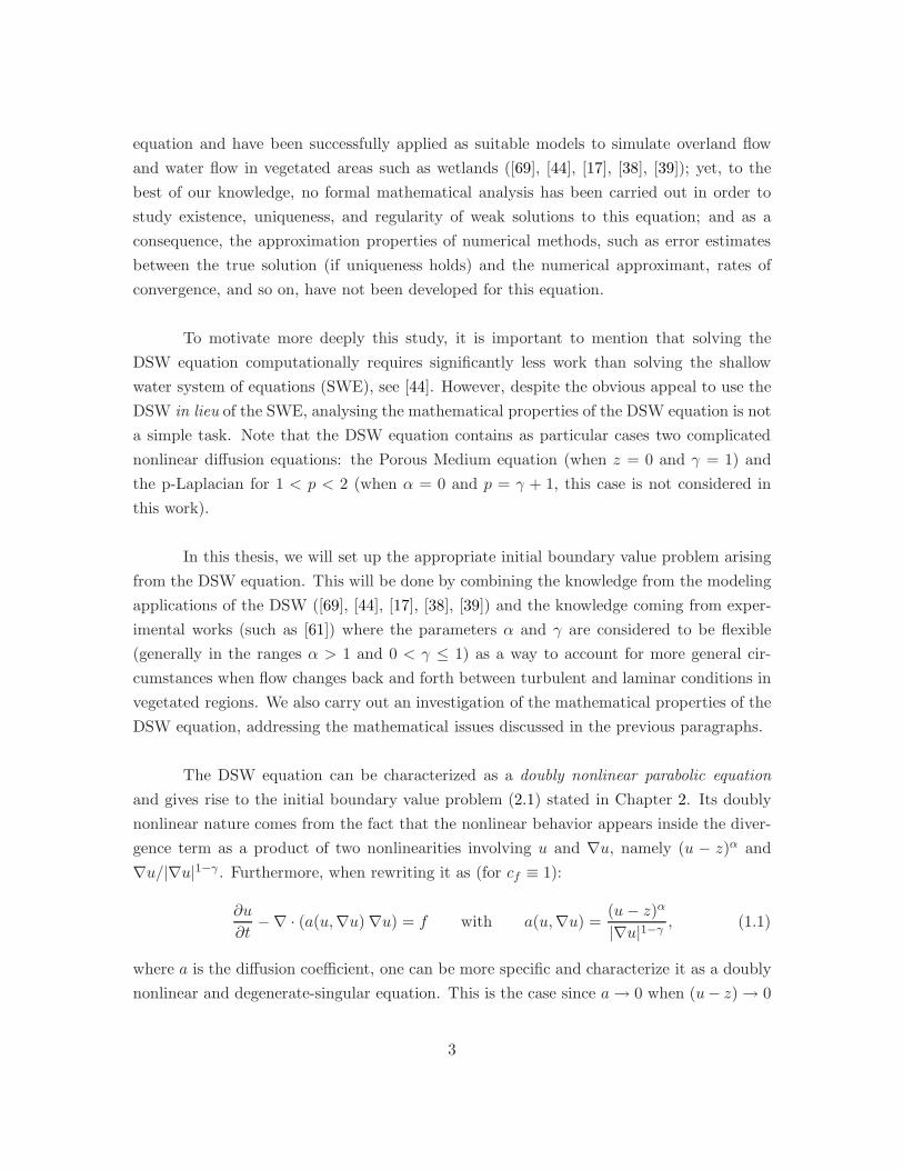
Water Surface

Y

X

H ( x , y )

Land Surface

Datum

h ( x , y )

z ( x ,y )

Figure 1.1: Land surface elevation is measured from the datum and represented by functionz(x,y), free water surface elevation by H(x,y) and the water depth by h(x,y).

and the 2-D depth-averaged momentum equations

∂(hu)

∂t+∂(hu2)

∂x+∂(huv)

∂y+ gh

∂H

∂x+

τbxρ0

= 0, (1.5)

∂(hv)

∂t+∂(huv)

∂x+∂(hv2)

∂y︸ ︷︷ ︸+ gh

∂H

∂y︸ ︷︷ ︸+

τbyρ0︸︷︷︸

= 0, (1.6)

inertial terms pressure friction

whereH(x, y; t) is the free surface elevation or hydraulic head, z is the bed surface, bathymetry

or land elevation, (See figure 1.1), h(x, y; t) = H(x, y; t) − z(x, y) is the water depth, f is a

source/sink (such as rain or infiltration), u(x, y; t) and v(x, y; t) are the x and y components

of the depth averaged horizontal velocity vector V , and τbx and τby are the x and y com-

ponents of the averaged boundary shear stress at the bed surface z, and ρ0 the reference

density of the fluid.

Further assumptions and simplifications of these equations lead to different overland

flow models. These models are generalizations of the one-dimensional open channel flow

approximations, which have been studied based on their capacity to simulate wave propa-

gation. See [55]. Mainly, two approximations are relevant to overland flow: the kinematic

wave and the diffusive wave approaches. The kinematic wave approach assumes that the

7

inertial terms as well as the pressure terms in the momentum equations (1.5) and (1.6) are

negligible when compared to the friction terms. The diffusive wave approach assumes that

only the inertial terms are negligible. Their applicability to one dimensional overland flow

was studied, for example by Ponce et al. in [54], who found conditions where both can

be used to simulate the physical phenomenon instead of the full SWE (also known as St.

Venant Equations).

Research teams have explored different models in order to capture the main features

of overland flow and water flow in vegetated areas in a computationally efficient manner.

Some recent studies addressing modeling techniques for these flow regimes, particularly

those arising in vegetated areas, can be found in [12] and the references therein. In this

section, however, we will mainly discuss those studies in which the use of the DSW equation

was successful in modeling overland flow and water flow in wetlands. For example, Xan-

thopoulos and Koutitas [69], as well as Hromadka et al. [44] validated a two-dimensional

dam-break model for flood wave propagation and flood plain study, respectively, based on

the diffusive wave approach. They concluded that the inertial terms are indeed negligi-

ble in situations where the bed surface is flat and derived the DSW equation under this

conditions. Hromadka et al. also concluded that the computational cost required to solve

the full St. Venant equations increases by 50% the cost required to solve the DSW equa-

tion. Xanthopoulos and Koutitas [69] solved the DSW equation using an explicit finite

difference (FD) scheme in Eulerian space and their results compared successfully with labo-

ratory experiments. They eventually used this approximation to model a plain in Northern

Greece. Hromadka et al. [44] solved the DSW equation using an integrated finite differ-

ence (IFD) formulation for regular and irregular triangle elements. They showed that the

two-dimensional diffusive approach could be used to predict a hypothetical dam break more

accurately than a one-dimensional model. Giammarco et al. [39] used a control volume fi-

nite element (CVFE) formulation to solve the DSW equation and showed that this approach

improves the classical Finite Element (FE) formulation since it is locally mass conservative.

They also showed that the CVFE represents the gradients better than the IFD. Feng and

Molz [38] derived an effective equation similar to the DSW equation using the diffusive

wave approach in order to model flow in wetlands. They solved such an effective equa-

tion using a fully implicit finite difference scheme in a regular mesh with square elements,

and using a Picard Iteration scheme to resolve the nonlinear terms in a fixed rectangular

domain with irregular wet boundaries. They also proposed an alternative friction formula

deduced empirically by Turner and Chanmeesri [61], see equation (2.5), which relates the

one-dimensional flow velocity to the one-dimensional friction bed slope for shallow flow of

8

water through non-submerged vegetation. Observations by Turner and Chanmeesri [61]

show that α > 1 and, in general 0 < γ ≤ 1. Bolster and Saiers [16] found that the value of

γ = 1 was the most suitable choice when calibrated with field measurements of hydraulic

heads. They used a predictor-corrector finite-difference scheme to solve the DSW equation

when modeling wetlands in the Shark River Slough in the Everglades in Florida. As a

last example of successful application of the DSW equation in order to model wetlands we

mention the work of Bauer et al. [11], who developed a numerical model using a finite

difference scheme to simulate the flow in a wetland system coupled with groundwater flow

in the Okavango Delta, in Botswana.

A related work using the SWE as a model for overland flow is the work by Zhang and

Cundy. In [73], they developed a fully dynamical model solving equations (1.4)-(1.6) assum-

ing particular forms of the friction shear stresses and using a MacCormack finite difference

scheme. Their model allows spatial variations of hillslope features, including surface rough-

ness, infiltration, and microtopography. Their main conclusion was that microtopography is

the dominant factor causing spatial variation in overland flow depth , velocity, and direction.

1.2.2 Doubly nonlinear diffusion equations

To the best of our knowledge, the DSW equation has not been studied in its general form

as presented in the initial boundary value problem (2.1) of Chapter 2. However, when to-

pographic effects are neglected (z ≡ 0) and zero-Dirichlet initial/boundary conditions are

assumed (∂Ω = ΓD), one can find a fairly extensive number of works that study doubly

nonlinear equations that are relevant to the DSW equation. See for example [50], [56],[41],

[6], [45]. Most of these works study alternative formulations of problem (2.1). These will

be explained in the subsequent paragraphs.

Two important particular cases of the DSW equation, that do not fall into the cat-

egory of doubly nonlinear diffusion equations that deserve to be mentioned are, the Porous

Medium Equation (PME) and the p-Laplacian. A comprehensive study of the PME can

be found in the book by Vazquez [62] and the references therein. For the time evolution of

the p-Laplacian the reader is referred to the book by DiBenedetto [31] and the references

therein. An interesting reference addressing a class of nonlinear diffusion equations in the

context of image processing and edge detection is [24]. The diffusion coefficients studied in

[24] depend purely on the gradient of the solution.

9

We proceed to summarize the most relevant results from studies of doubly nonlinear

diffusion equations existing in the literature that can be applied to the DSW equation

when topographic effects are ignored. In order to do so, we will introduce an alternative

formulation that has been studied before. This formulation will be used throughout this

section and in Chapter 3 of this thesis and is given by

∂φ(v)

∂t− ηγ ∇ ·

( ∇v|∇v|1−γ

)= f on Ω × (0, T ]

v = 0 on ∂Ω × [0, T ]

v = v0 on Ω × t = 0

(1.7)

where Ω is either Rn or an open (and in most cases bounded) subset of R

n, η is a posi-

tive constant, and the function φ(s) ∈ C0,η(R) is an odd function satisfying the following

properties:

(i) |φ(s)| ≤ |s|η for 0 < η ≤ γ < 1, with equality for |s| ≥ R for some R ≥ 0

(ii) φ(s) is a concave increasing function for s ≥ 0.

Note that with the change of variables defined by u = φ(v), problem (1.7) is transformed

into

∂u

∂t− ηγ ∇ ·

( ((φ−1)′(u)

)γ ∇u|∇u|1−γ

)= f on Ω × (0, T ]

u = 0 on ∂Ω × [0, T ]

u = u0 on Ω × t = 0

(1.8)

Now, choosing

0 < η =γ

α+ γ< 1, and φ(s) =

s

|s|1−η(1.9)

we can obtain the explicit expression for

(φ−1)′(s) = (1 + θ)|s| θ where θ =1 − η

η=α

γ(1.10)

which yields the following equation

∂u

∂t−∇ ·

(|u|α ∇u

|∇u|1−γ

)= f. (1.11)

The previous manipulations show, at least formally, that nonnegative solutions of problem

(1.7) are solutions of the DSW equation for flat topographies. Most of the results found in

10

the literature address the IBVP (1.7).

1.2.2.1 Existence of solutions

Lions [50] introduced the techniques of compactness and monotonicity later utilized in the

subsequent works in the proofs of existence for problem (1.7). Raviart [56], and Grange

and Mignot [41] prove the existence of weak solutions to problem (1.7), provided Ω is an

open and bounded subset of Rn, constructing approximate solutions using implicit finite

differences in time and passing to the limit by means of compactness and monotonicity. In

[56] Raviart worked directly with problem (1.7), and in [41] Grange and Mignot extended

such results to the abstract setting of equations of the type:

∂Bu

∂t+Au = f

where A and B denote the subdifferentials of convex functionals. Their analysis is based on

the essential restriction that these functionals must be continuous on appropriate Banach

spaces. Bernis further extends these results to the case when Ω is any open set of Rn in [14].

Another relevant reference is [15], where Blanchard and Francfort address the semi-abstract

problem∂

∂tb(u) −∇ · (DΦ(∇u)) = f

where b is a locally Lipschitz function and may grow faster than any power function at

infinity, and Φ is a C1 convex functional with specific coercivity assumptions. They obtain

existence and comparison results with the aid of a Galerkin approximation technique which

uses truncation-penalization of the time nonlinearity and a priori estimates through con-

vex conjugate functions. An important work addressing quasilinear and doubly nonlinear

parabolic equations is found in Alt and Luckhaus [3].

1.2.2.2 Comparison principles and uniqueness

In [6], Bamberger studies the existence of particular solutions to problem (1.7) which are

the limit of solutions fortes i.e. solutions that have the property φ(u)t ∈ L1(0, T, L1(Ω)).

Bamberger refers to this kind of solutions as limite de solutions fortes. In addition, he

presents a very concise exposition of a comparison principle between solutions that are

limite de solutions fortes and uses this result to find uniqueness. See Section 3.3.

11

1.2.2.3 Regularity

When topographic effects are neglected (z ≡ 0) and zero-Dirichlet initial/boundary condi-

tions are assumed (∂Ω = ΓD) Problem (2.1) can also be re-written in the form:

∂u

∂t−∇ ·

(|∇um|γ−1∇um

)= f (1.12)

with m = 1 + α/γ. Esteban and Vazquez [35] studied this equation in 1-D for the Cauchy

problem (Ω = R). They study the local velocity of propagation

V (x, t) = −vx|vx|γ−1

where v is the nonlinear potential defined as:

v =

mγ

mγ − 1u

mγ−1γ if mγ 6= 1

1

γlog u if mγ = 1

Recall that in the DSW equation, it is assumed that mγ = α+ γ > 1. In their work, they

base their approach on the existing theory for the Porous Medium Equation and find the

estimate

Vx ≤ 1

γ(m+ 1) t.

Using the previous estimate as the main tool, they construct a theory for the Cauchy

problem with nonnegative, integrable initial data. In particular, they address the following

questions:

• Existence, uniqueness and regularity of strong solutions,

• Existence and regularity of free boundaries,

• Asymptotic behaviour of solutions and free boundaries.

In [45], Ishige gives a sufficient condition for the growth order of the initial data at infinity

for the existence of weak solutions of the Cauchy problem (Ω = R) (1.7).

1.2.2.4 Additional properties of solutions

Some interesting facts about nonnegative solutions to problem (1.7) are:

• Finite speed of propagation. Indeed, Barenblatt constructed a class of self-similar

source type solutions for the Cauchy problem (Ω = R) which have the property that

12

their supports propagate in time with finite speed, when α+ γ > 1. See [7].

• Extinction property. In [6], using simple arguments, Bamberger exhibits that for

f = 0, nonnegative solutions to the zero-Dirichlet boundary value problem (Ω ⊂ R,

bounded) become zero in finite time.

• Traveling waves. It is worthwhile mentioning that an interesting example of traveling

wave type solutions

u(x, t) = U(t− n · x) with U(s) = 0 for s > 0,

to the zero-Dirichlet boundary value problem (Ω ⊂ R, bounded) is shown in [6] for

the case when η > γ (equivalently α < 1 − γ). In the DSW equation this case does

not arise since α > 1 and 0 < γ ≤ 1.

Other properties of solutions including nonexistence of global nonnegative solutions and

blow up solutions can be found in [14] and [45] respectively, for particular choices of the

parameters η and γ that do not happen in the DSW equation case.

1.2.3 Numerical methods for nonlinear parabolic problems

As mentioned before, finite difference schemes and finite element techniques have been im-

plemented to approximate the solution of the DSW equation and have been used successfully

to simulate water flow in shallow systems in [69], [44], [39], [38], [61], [11]. However, no

formal numerical analysis has been carried out in order to show that the proposed methods

converge in some sense to the true solution of the IBVP (2.1) . This is not surprising given

the complexity of the general formulation of the IBVP (2.1) and the lack of analytical tech-

niques to prove for example uniqueness of solutions in the presence of topographic effects.

Generally speaking, numerical schemes to solve parabolic problems have been widely

explored. The most important methodologies utilized in the past are two: finite difference

schemes and finite element methods. The early works of Courant, Friedrichs and Lewy [29]

served as a starting point in the development of finite difference schemes, where the ap-

proximate solution of the equation is constructed by solving algebraic difference equations

at given mesh points in the domain at each time step. See, for example, [59]. Later on,

the works of Wheeler [67] and Douglas and Dupont [32] played a key role in the study of

approximate solutions (globally throughout the domain) to nonlinear diffusion equations

using the Galerkin finite element method. In the finite element method an approximate

solution is constructed as a linear combination of so-called basis functions of a linear space

13

by solving a discrete variational formulation derived directly from the partial differential

equation at hand. Loosely speaking, the Galerkin finite element has proved to be supe-

rior when numerically solving partial differential equations in complex domains or when

the solution lacks smoothness. References such as [18] and [34] describe the mathematical

background and applications of this method. Of particular interest is the book by Thomee

[60] and the references therein, where a comprehensive account of the mathematical theory

of Galerkin finite element methods as applied to parabolic partial differential equations is

presented. The Galerkin finite element method, both in its continuous and discontinuous

versions, will be the basis for this thesis work.

Within the context of the continuous Galerkin finite element method, relevant works

approximating degenerate parabolic equations include for example: [53], [72], [57], [42], [37],

and [4]. Even though the DSW equation (as presented in Chapter 2) does not fall into the

set of equations solved in these references, they provide important techniques that will

be explored in this thesis. In particular, in [53], Nochetto and Verdi present a numerical

method to approximate degenerate parabolic problems, based on the finite element method,

similar to the one used in this thesis work. In their study they analyze equations of the

form∂u

∂t−∇ · ( ∇v + b(r(v)) ) + f(r(v)) = 0, u ∈ m(v), (1.13)

where m(v) is a maximal monotone graph in R×R possibly with a singularity at the origin

(m′(0) = ∞). Stefan type, nonstationary filtration type, and porous-medium type degen-

erate parabolic equations can be written in the form (1.13). One may replace r(v) by v

for intuition purposes. In cases when singularities in m appear, Nochetto and Verdi use a

smoothing procedure similar to the one that will be used in Chapter 3. In their approxima-

tion strategy, they construct a numerical scheme that approximates a regularized problem

obtained by replacing m in (1.13) by a smooth function mǫ with maximal slope equal to

1/ǫ, for some regularization parameter ǫ > 0. Then they discretize this regularized prob-

lem in space and time to compute the regularized numerical approximation Uhǫ (t). Finally,

roughly speaking, they show global error estimates between the solution u(t) of (1.13) and

the regularized numerical approximation Uhǫ (t). Their method will be discussed again in

Chapter 4 when we introduce the numerical strategy proposed in this thesis work.

In [72], Yong and Pop present a methodology to numerically solve porous medium-type

equations based on the maximum principle. In their approach they locally perturb the

(initial and boundary) data instead of the nonlinear diffusion coefficients to keep solutions

away from degeneracy. In [57], Rulla and Walkington obtain optimal spatial error estimates

14

for degenerate parabolic problems by using semigroup theory. However, in their approach,

they do not discuss the numerical techniques to solve these degenerate equations. This

is the case as well in [42], where Hansen and Ostermann focus their study in improving

the temporal error estimates of porous medium-type equations by using high order implicit

Runge-Kutta methods. In [37], Evje and Karlsen analyse discrete approximations of weak

solutions of bounded variation (BV), in space and time, to doubly nonlinear parabolic equa-

tions. Their approach is carried out in the framework of BV because weak solutions of the

equations they study are, in general, not uniquely determined by their data. The kind of

doubly nonlinear parabolic equations presented in [37] differ from the DSW in the fact that

topographic effects cannot be incorporated in their formulation. Finally, in [4], Arbogast

et al. develop and analyse two mixed finite element approximations to obtain approxi-

mate solutions of a nonlinear, degenerate advection diffusion equation arising in petroleum

reservoir and groundwater aquifer simulation. The diffusion coefficient of the equation they

study does not contain nonlinearities with respect to the gradient of the solution. For com-

pleteness, we refer the reader to [8], [48] and the reference therein for numerical studies

addressing equations with diffusion coefficients that depend purely on the gradient of the

solution, such as the time evolution of the p-Laplacian.

In Chapter 5, the local discontinuous Galerkin (LDG) method will be introduced as

an appropriate setting to handle complex geometries as well as a natural technique that

allows the easy coupling of the DSW model with other surface water models (such as the

SWE) and other subsurface flow models (such as Darcy’s flow or other infiltration models).

The LDG method is one of many discontinuous Galerkin (DG) methods. In these methods,

continuity across elements is not enforced in the linear space where the basis functions live,

thus giving rise to “broken” or discontinuous approximate solutions. This is a major differ-

ence with the continuous Galerkin finite element method. For a review on the development

of discontinuous Galerkin methods see the book by Cockburn et al. [27].

In the context of elliptic and parabolic problems, the DG methods emerged from

the interior penalty (IP) methods. The IP methods were originally devised as a means to

impose Dirichlet boundary conditions weakly rather than incorporating the boundary con-

ditions into the finite element space [52]. This idea was further generalized, at the element

level, by enforcing continuity across elements weakly in [68]. The development of these ideas

in the context of elliptic equations can be found in the Chapter: “Discontinuous Galerkin

Methods for Elliptic Problems” in [27].

15

The LDG method was introduced by Cockburn and Shu in [28] as an extension, to

general convection-diffusion problems, from the numerical techniques introduced by Bassi

and Rebay in [10] to solve the compressible Navier-Stokes equations. One of the basic ideas

in the LDG method is to rewrite, say the parabolic equation at hand, as a degenerate first

order system of equations where both u and ∇u (= q) are now considered as independent

unknowns. This strategy is also present in methods based on a mixed formulation. In the

LDG method, one further discretizes the resulting first order system using particular DG

techniques. Details about the method set up in the context of elliptic problems can be

found in [22]. Some general characteristics of the DG methods are the following:

• They can easily handle various shapes in different elements across the domain, as well

as local spaces of different types (orders). This is the case since continuity is not

enforced strongly across elements.

• The previous property makes these methods suitable to handle structured and un-

structured meshes in domains with general geometries.

• Their high degree of locality makes them highly parallelizable.

• They are element-wise conservative (This statement is meaningful when modeling

(nonlinear) conservation laws).

• They are ideally suited for hp-refinement (or hp-adaptivity).

Particular to the LDG method studied in this thesis work, the approximation to u, and the

approximation to each of the components of q belong to the same approximation spaces,

making the coding simpler than in the standard mixed methods. Also in the so-called

numerical flux, introduced to properly define the values of the fluxes across all element

boundaries, u will not depend on q making it possible for the local variable q to be solved

in terms of u. These characteristics will be described in detail in Chapter 5.

Works addressing the properties of the LDG method in the context of convection diffusion

problems include for example: [28], [26], [23], and [1]. The applicability of the LDG method

has been explored for example, for elliptic problems in [5], for nonlinear diffusion problems

in [19], for Richard’s equation (a nonlinear parabolic equation) in [49], and for PDE’s with

higher order derivatives in [70] and [71].

16

1.3 Accomplishments

The main results of this dissertation can be summarized as follows:

• In section 1.2 of this Chapter, we present a collection of studies where the DSW has

been used as a suitable model for shallow water flow in particular flow regimes; we

describe the most relevant results in studies of doubly nonlinear diffusion equations

existing in the literature that can be applied to the DSW equation when topographic

effects are ignored (i.e., when z 6= 0); and finally, we give an overview of some relevant

works addressing the numerical approximation of solutions to nonlinear parabolic

equations.

• In Chapter 2, we state the appropriate initial boundary value problem arising from

the DSW equation. This is done by combining the knowledge from the modeling

applications of the DSW and the knowledge coming from experimental works where

the parameters α and γ are considered to be flexible (generally in the ranges α > 1

and 0 < γ ≤ 1) as a way to account for more general circumstances when flow changes

back and forth between turbulent and laminar conditions in vegetated regions. An

alternative, simple, and intuitive derivation of the DSW equation in the context of

shallow water flows is obtained.

• In Chapter 3, an original and constructive proof of existence of weak solutions to the

zero-Dirichlet initial/boundary value problem (2.1) using the Faedo Galerkin method

is presented, for situations when topographic effects are ignored. Proofs for some regu-

larity results are also shown, including conditions for which a comparison principle for

solutions can be established and thus conditions for which uniqueness of solutions can

be ensured. The ideas presented in this Chapter are the result of a joint collaboration

with Ricardo Alonso.

• In Chapter 4, a numerical method based on the continuous Galerkin finite element

method is proposed. Conditions, based on physical consistency, for which a priori

error estimates and convergence rates can be ensured, are described for this method.

The results of numerical experiments in 1-D, using a lumped mass finite element code

(in Matlab), are reported. The main objectives of these experiments include:

– to verify the convergence rates of the method,

– to numerically simulate water depth profiles and hydrographs in unsteady flow

conditions. The numerical results matched the real measurements obtained in

an experiment conducted by Iwagaki [46].

17

– to investigate qualitative properties of solutions to the DSW equation when to-

pographic effects are incorporated.

• In Chapter 5, the local discontinuous Galerkin method is introduced along with con-

ditions for which a priori error estimates and convergence rates can be ensured. The

results of numerical experiments in 2-D, using an LDG finite element code (in FOR-

TRAN) implemented to solve the DSW equation and aiming at verifying the modeling

qualities of the DSW equation in the context of shallow water modeling, are presented.

These include: the simulation of a dam break problem, and the simulation of water

flow in an inclined and vegetated region.

18

Chapter 2

The DSW Equation and

Preliminaries

The outline of this Chapter is the following. In section 2.1, we will introduce the initial

boundary value problem associated with the DSW equation, following the notation found in

the mathematical literature on Partial Differential Equations (PDE), see for example [36].

Throughout this dissertation, we will consistently use this notation except for two sections:

section 1.2.1 and section 2.2, where the notation commonly used in the context of shallow

water hydrodynamics will be utilized, see for example [65]. In 2.2, a derivation of the DSW

equation from the shallow water system of equations will be provided. For consistency, we

provide further details about the mathematical notation used in this dissertation in section

2.3. Well known results in interpolation theory will be listed for completeness in section

2.4.

2.1 The initial-boundary value problem

The DSW equation gives rise to the following initial/boundary-value problem prescribed

for any fixed T > 0

∂u

∂t−∇ ·

((u− z)α

|∇u|1−γ∇u

)= f on Ω × (0, T ]

u = u0 on Ω × t = 0(

(u− z)α

|∇u|1−γ∇u

)· n = g

Non ∂Ω ∩ Γ

N× (0, T ]

u = gD

on ∂Ω ∩ ΓD× (0, T ]

(2.1)

19

where Ω is an open, bounded subset of Rn (n = 1, 2) and ΓN and Γ

Dare subsets of ∂Ω ∈ C1

such that ∂Ω = ΓN

+ ΓD. Also f : Ω × (0, T ] → R, u0 : Ω → R, g

N: Γ

N× (0, T ] → R,

gD

: ΓD× (0, T ] → R are given functions, z : Ω → R

+ is a positive time independent

function, 0 < γ ≤ 1, 1 < α < 2, and u : Ω × [0, T ] → R is the unknown. Here | · | : Rn → R

refers to the Euclidean norm in Rn.

As mentioned in Chapter 1, problem (2.1) is characterized as doubly nonlinear since

the nonlinear behaviour appears inside the divergence term as a product of two nonlinearities

involving u−z and ∇u, namely (u−z)α and ∇u/|∇u|1−γ . In fact, when the DSW equation

is re-written as

∂u

∂t−∇ · (a(u,∇u) ∇u) = f with a(u,∇u) =

(u− z)α

|∇u|1−γ,

where a is the diffusion coefficient, one can be more specific and characterize it as a doubly

nonlinear and degenerate-singular equation for the given choice of 0 < γ ≤ 1, and 1 < α < 2.

This is the case since a → 0 when (u − z) → 0 and a → ∞ when ∇u → 0. In the context

of shallow water modeling, u(x, t) represents the surface water elevation in the position x

at time t, the positive time independent function z(x) describes the bathymetry of the bed

surface throughout the domain and introduces the commonly called topographic effects into

the model.

The types of physical boundary conditions appropriate for this model are two, a

prescribed water depth gD

on ΓD, and/or a prescribed water flux g

Non Γ

N. The first

one corresponds to a Dirichlet type boundary condition and it is mostly used to model an

infinite source of water on the boundary ΓD. The second one corresponds to a Neumann

type boundary condition and it is the most natural choice to model water flux through a

boundary ΓN

.

2.2 Derivation from the shallow water equations

Models for surface water flows are derived from the incompressible, three-dimensional

Navier-Stokes (NS) equations, which consist of momentum equations for the three velocity

components and a continuity equation. Depending on the physics of the flow, scaling ar-

guments are used in order to obtain effective equations for the problem at hand. Equation

(2.1) is a simplified version of the two-dimensional shallow water equations called the dif-

20

fusive wave or zero-inertia approach. This equation is commonly derived by neglecting the

inertial terms in the horizontal momentum equations and substituting the bottom slope in

Manning’s formula by the water surface slope. This approach is shown in [38], [69], [44],

[17], and [39]. In the following paragraphs we provide an intuitive, concise and equally valid

derivation following a more empirical approach, such as the one used to derive the Porous

Medium Equation in section 2 of [62].

Recall that in shallow water theory, the main scaling assumption is that the vertical scales

are small relative to the horizontal ones. This approximation reduces the vertical momentum

equation to the hydrostatic pressure relation

∂p

∂x3

= ρg (2.2)

where g is the gravitational constant, x3 the vertical coordinate and p the pressure, and

leaves us with two effective momentum equations in the horizontal direction. Upon vertical

integration of the NS equations, we obtain two depth-averaged momentum equations and

a depth-averaged continuity equation. These resulting equations are called the 2-D shallow

water equations. For a detailed description of shallow water hydrodynamics see [65] and [63].

When combining the depth-averaged continuity equation with the free surface boundary

condition, one obtains the mass balance equation

∂h

∂t+ ∇ · (hV ) = f, (2.3)

where h(x, t) = H(x, t)− z(x) is the water depth, H(x, t) is the free water surface elevation

or hydraulic head, z(x) is the bed surface, bathymetry, or land elevation, V (x, t) is the

depth-averaged velocity, and f(x, t) is a source/sink (such as rainfall or infiltration).

In open channel flow theory, empirical laws such as Manning’s formula or Chezy’s formula

have been observed to successfully describe the dynamics of water flow in regimes when

fluid motion is dominated by gravity and balanced by the bottom boundary shear stress.

See [47] or chapter 11 in [30]. Examples of open channel flow include water flow in rivers,

in partially full drains and surface runoff. Manning’s and Chezy’s formulas relate the mean

velocity of the flow V with the so-called hydraulic radius1 R and the bottom slope S through

1The hydraulic radius for open channels is calculated as R = A/ω, where A is the cross section of thechannel, and ω is the wetted perimeter. Note that for a rectangular cross section with base L and depth h,R = hL/(L + 2h) ∼ h when L >> h.

21

a friction coefficient cf in the following way:

V =1

cfRα−1Sγ , (2.4)

for particular choices of α and γ. For Manning’s formula2 α = 5/3 and γ = 1/2, and for

Chezy’s formula α = 3/2 and γ = 1/2. When one multiplies equation (2.4) by the hydraulic

radius R, one obtains an equivalent relation in terms of the water discharge Q

Q = RV =1

cfRαSγ . (2.5)

The discharge-depth equation (2.5) is a generalization of both Manning’s formula or Chezy’s

formulas and was proposed in [61] as a way to account for more general circumstances when

flow changes back and forth between turbulent and laminar conditions. This is the case,

for example, in water flow in vegetated areas. In [61], the authors study equation (2.5) as

a prediction model for shallow water flow in vegetated areas based entirely on empirical

procedures. In their study they conclude that equation (2.5) with flexible coefficients α and

γ results in a broader and better model than the particular Manning’s formula. Experimen-

tally, they reported values in the ranges 1 ≤ α ≤ 2 and 0 < γ < 1. These values motivate

the ranges of α and γ in the present work. Further assumptions in open channel theory

that justify the application of velocity-depth equations like (2.4) include:

• the approximation of the hydraulic radius R by the water depth h in (2.4) and (2.5),

• the assumption that the slope of the bathymetry is small, and

• the assumption that the bottom slope is comparable to the free water surface slope.

In the diffusive wave approximation, one makes use of the previous assumptions, and extends

the scaling of the mean flow velocity V with respect to R and S in (2.4), to the depth-

averaged velocity V (x, t) in (2.3) along the direction of the flow. This is done in the

following way: since the flow is assumed to be dominated by gravity, the direction of the

flow will be along the unitary vector ∇H/|∇H| (recall equation (2.2)), and thus, equation

(2.4) is transformed into

V = −hα−1

cf

∇H|∇H| |∇H|γ = −(H − z)α−1

cf

∇H|∇H|1−γ

, (2.6)

The DSW equation is obtained from substituting the particular form of the depth-averaged

2For a derivation of Manning’s formula based on the phenomenological theory of turbulence see [40].

22

horizontal velocity given by (2.6), into equation (2.3)

∂H

∂t−∇ ·

((H − z)α

cf

∇H|∇H|1−γ

)= f(t, x), for (t, x) ∈ R

+ × R2, (2.7)

The assumptions made to obtain the DSW equation suggest that it may be suitable to serve

as a model in low-to-moderate velocity-flow regimes. See section 2 of [39] and the references

therein.

Remark 2.2.1. In hydrological systems, z describes the bed surface over which water flows,

thus, in physically meaningful situations one assumes that ∇z must be bounded. This in

turn implies, in physically meaningful solutions, the boundedness of ∇H. This is an extra

assumption that will be used in the numerical error analysis that aligns well with the physics

of the associated problem.

Remark 2.2.2. In this context, equation (2.7) makes sense physically only if H − z ≥ 0.

It is with this in mind that we will not pay attention to the approximation of negative

solutions of (2.1). Note that in writing (2.1) we have assumed that cf (x) ≡ 1.

Remark 2.2.3. Note that if one identifies the water elevation H with the hydrostatic

pressure p, the expression that relates the velocity and the water elevation gradient (2.6)

becomes a nonlinear version of the empirical Darcy’s law for gas flow through a porous

medium. Indeed, flow in vegetated areas such as wetlands can be understood as a flow

through a porous medium.

One interesting fact about solutions of the DSW is the following. When one sees the DSW

equation as a conservation law with respect to the depth u∗ = u− z, it becomes

∂u∗

∂t−∇ · ( u∗V ) = f,

where the horizontal velocity V is given by (2.6), and its magnitude is

|V | =|u∗|α−1

cf|∇u|γ ,

which indicates that at the free boundary (interface between regions where u∗ > 0 and

u∗ = 0) or any place in the domain where the depth of the water u∗ is zero, the magnitude

of the velocity is zero since α > 1.

Remark 2.2.4. For studies addressing the applicability of the DSW equation as a model to

simulate shallow water flow, instead of the full Saint Venant (or Shallow Water) equations

in experimental and real life settings we refer the reader, for example, to: in the 1 -D case

23

the works of Ponce et al. [55] and [54], and in 2-D cases the references mentioned in section

1.2.1.

2.3 Notation

We will use the standard notation introduced in [36]. Let X be a real Banach space, with

norm ‖·‖. The symbol Lp(0, T ;X) will denote the Banach space of all measurable functions

u : [0, T ] → X such that

(i) ‖u‖Lp(0,T ;X) :=(∫ T

0 ‖u(t)‖p)1/p

<∞, for 1 ≤ p <∞, and

(ii) ‖u‖L∞(0,T ;X) := ess sup0≤t≤T ‖u(t)‖ <∞.

We will denote with C([0, T ];X) the space of all continuous functions u : [0, T ] → X such

that

‖u‖C(0,T ;X) := max0≤t≤T

‖u(t)‖ <∞.

Let u ∈ L1(0, T ;X), we say v ∈ L1(0, T ;X) is the weak time derivative of u, denoted ut = v,

provided ∫ T

0ψt(t) u(t) = −

∫ T

0ψ(t) v(t)

for all scalar test functions ψ ∈ C∞0 (0, T ). Throughout the paper, W 1,p(0, T ;X) will denote

the space of all functions u ∈ Lp(0, T ;X) such that ut exists in the weak sense and ut ∈Lp(0, T ;X) with the norm

‖u‖W 1,p(0,T ;X) :=

(∫ T

0‖u(t)‖p + ‖ut(t)‖p

)1/p

(1 ≤ p <∞),

ess sup0≤t≤T

(‖u(t)‖ + ‖ut(t)‖) (p = ∞).

For 1 ≤ p ≤ +∞, we will denote its conjugate as p∗ i.e., 1/p+1/p∗ = 1. For any measurable

set E ⊂ Ω and real valued vector functions u ∈ Lp(E) and v ∈ Lp∗(E) we will denote the

duality pairing between u and v as

(u, v)E :=

∫

Eu · v.

For simplicity, we use (u, v) := (u, v)Ω. Similarly, we will denote the duality pairing between

u ∈ W−1,p∗(Ω) and v ∈ W 1,p0 (Ω) as 〈u, v〉. Recall that the elements of W−1,p∗(Ω) are the

distributions that have continuous extension to W 1,p0 (Ω). These spaces are characterized in

24

the following way: if u ∈ W−1,p∗(Ω), then there exists functions f0, f1, · · · , fn in Lp∗(Ω)

such that

〈u, v〉 = (f0, v) +

n∑

i=1

(f i, vxi).

Throughout the paper, C will be a generic constant with different values and the explicit

dependence with respect to parameters will be written inside parenthesis.

2.4 Interpolation theory results. Continuous case

For Lemmas 2.4.1, 2.4.2, 2.5.1, and 2.5.2, we will consider τ to be a quasi-uniform triangu-

lation of Ω into elements Ei, i = 1, ...,m, with diam(Ei) = hi and h = maxi(hi). M(= Pk)

will denote a finite dimensional subspace of H10 (Ω) defined on this triangulation consisting

of piecewise polynomials of degree at most k and K0 will denote a constant independent of

h and v.

Lemma 2.4.1 (Interpolation error). Let u ∈ Hk+1(Ω), then there exists u ∈ M, projection

of u, defined by ∫(u− u)v = 0 ∀ v ∈ M (2.8)

with the following property:

‖u− u‖Hs(Ω) ≤ C hk+1−s ‖u‖Hk+1(Ω)

where 0 ≤ s ≤ k.

Proof. See section 4.4 in [18].

Lemma 2.4.2 (Inverse inequalities). Let v ∈ M then, there exists a constant K0 indepen-

dent of h and v such that

‖v‖L∞(Ω) ≤ K0h−1‖v‖L2(Ω) and ‖∇v‖L∞(Ω) ≤ K0h

−1‖∇v‖L2(Ω)

Proof. See section 4.5 in [18].

Remark 2.4.1. Lemma 2.4.1 implies that for a subspace M = P1 consisting of piecewise

linear polynomials,

‖u−u‖L2(Ω) ≤ C h2 ‖u‖H2(Ω) and ‖∇u−∇u‖L2(Ω) ≤ C‖u−u‖H1(Ω) ≤ C h‖u‖H2(Ω)

(2.9)

These inequalities will be useful in section 4.4.

25

2.5 Interpolation theory results. Discontinuous case

In Chapter 5, a discontinuous Galerkin method will be introduced where the need to have a

possibly broken approximate solution across elements may arise. In such cases, the results

of Lemmas 2.4.1 and 2.4.2 will be valid when applied to each element Ωe separately, and as a

consequence, they will also be valid when applied to the union (or the sum over elements).

However, we require two extra Lemmas in order to bound the errors associated to the

element boundary integrals. The following lemmas address this issue.

Lemma 2.5.1 (Trace interpolation error). Let u ∈ Hk+1(Ω), then there exists u ∈ M,

interpolant of u with the following property:

‖u− u‖Hs(∂Ωe) ≤ C hk+ 12−s ‖u‖Hk+1(Ωe)

where 0 ≤ s ≤ k.

Proof. See [25].

Lemma 2.5.2 (Trace inequality). Provided s ∈ (M)n, where n = 1, 2, is the space dimen-

sion, then there exists a constant C independent of the mesh size h such that

‖s‖L2(∂Ωe) ≤ C h−12 ‖s‖L2(Ωe)

Proof. See [25].

26

Chapter 3

Existence, Regularity and

Uniqueness of Weak Solutions

As mentioned in Chapter 1, the study of existence, uniqueness, and regularity of weak so-

lutions to the IBVP (2.1) remains an open problem. However, when topographic effects are

ignored (z ≡ 0) and for nonnegative solutions, the IBVP (2.1) can be transformed into the

IBVP (1.7). The overall strategy of this Chapter is to study in depth the IBVP (1.7) and

then interpret the findings in terms of the IBVP (1.8) through corollaries and observations.

Recall that the IBVP (1.8) is a generalization (when z ≡ 0) of the IBVP (2.1) and that

nonnegative solutions of the IBVP (1.8) coincide with nonnegative solutions of the IBVP

(2.1) when φ(s) is chosen as in (1.9). The ideas presented in this Chapter were conceived

in joint collaboration with Ricardo Alonso and resulted in the publication of [2].

The outline of this Chapter is the following. In section 3.0.1, we describe the rele-

vance of the analysis carried out in this Chapter in the context of shallow water modeling.

In section 3.0.2, we provide some intuition about the regularization technique used in the

proof of existence. The notion of weak solution and its precise meaning in this analysis is

introduced in section 3.0.3. In section 3.1, we present a concise and constructive proof of

existence of weak solution to the alternative problem (1.7) using techniques originally intro-

duced by Lions [50] and further developed for quasi-linear parabolic equations by Alt and

Luckhaus [3] and for doubly nonlinear equations by Bernis[14]. This constructive method

provides a natural setting for a computational method to find approximate solutions to

problem (1.7), further described in Chapters 4 and 5, within the framework of finite el-

ement techniques. In this proof of existence, instead of following the time discretization

approach established in [56] and [41], we take advantage of the continuous in time evolu-

27

tion of the appropriate Banach space norms of the approximate solutions and find a priori

estimates for them. This is a standard technique proposed in [50] that does not require

any truncation-penalization technique as the one used in [15]. The approximate solutions

constructed in this proof are solutions fortes in the sense of Bamberger [6], and thus, they

and their limit will satisfy all the results presented in [6]. In particular, the result on unique-

ness of limite de solutions fortes in [6] will ensure that the numerical schemes analysed in

Chapters 4 and 5 will converge to a unique solution. It is important to note that in this

study we do not require the nonlinearity in time to be locally Lipschitz as in [15].

In addition, we include a concise argument to prove the L∞ control and integrability prop-

erties of the time derivative of solutions in section 3.2. Although these results have been

studied, the regularity arguments we present in this thesis are hard to find in the literature

and provide insight on the complexities of the equation.

For completeness, in section 3.3, we include the proof of a comparison result mentioned in

[6], and use it to prove uniqueness, nonnegativity and stability of the proposed approxima-

tion scheme. In the last section, we present possible avenues of research as well as a brief

discussion of this Chapter.

3.0.1 The obstacle problem

It is important to mention at this point that, within the shallow water modeling context,

a complete analysis of the DSW equation and thus problem (2.1), should be posed as an

obstacle problem, in other words, any physical solution u of problem (2.1) should be greater

or equal than the topography z (in this Chapter considered flat) regardless of the sign of the

input f (possibly negative when modeling physical processes such as infiltration or evapo-

ration). In other words, one should study the time evolution of the positivity set of u− z,

denoted by (u − z)+, and as a consequence, one should also characterize the properties of

the free boundary (interface between regions where u = z and u > z). As stated in the

previous paragraphs, this is not the way we will analyse problem (2.1). Furthermore, note

that in the approach followed in this Chapter, a solution u of problem (1.7) (recall equa-

tion (1.11)) could be negative, and thus physically inconsistent. As a note in favor of our

approach, however, we will show in section 3.3 that the nonnegativity of f will imply the

nonnegativity of a solution u of problem (1.7), for any physically consistent initial condition

u0 ≥ 0. Furthermore, the analysis presented in this Chapter will be physically relevant for

all cases when the combination of inputs f (infiltration, evaporation, and rainfall) are such

that u ≥ 0.

A classical example of an obstacle problem approach can be found in [62] for the Porous

28

Medium Equation, where free boundary issues need to be explicitly addressed. A closely

related one dimensional obstacle problem formulation can be found in [20] for a doubly

nonlinear parabolic equation arising in ice sheet dynamics. In general, the theory of free

boundaries is an important and difficult subject of mathematical investigation. In particu-

lar, the free boundary theory for doubly nonlinear equations is an area of research far from

being complete.

3.0.2 Regularization technique

Since the regularization technique used in the the proof of existence inspires the formulation

of the numerical methods used to approximate solutions of the DSW equation in Chapters 4

and 5, we will elaborate on it briefly. The key idea of this regularization technique is to find

a solution to problem (1.7) when φ is replaced by a Lipschitz function φreg approximating φ

uniformly, such that |φreg| ≤ |φ|. Then, the goal is to show that a solution to problem (1.7)

can be found as a limit of these regularized solutions. Similar regularization techniques have

been used in the approximation of solutions of degenerate parabolic equations as described

in section 1.2.3. These include: [53], [57], [64], [9], [72].

This regularization process can be interpreted as enforcing some sort of ellipticity

condition for the original problem (2.1) (by means of problem (1.8)), since it is a regular-

ization for small values of u where the degenerate character of problem (2.1) arises. To

support such interpretation, we plotted in Figure 3.1, functions φ(x), φ−1(x) and (φ−1)′(x)

without the Lipschitz property, and functions φreg(x), φ−1reg(x) and (φ−1

reg)′(x) with the Lip-

schitz property. In particular, the plot of (φ−1reg)

′(x) shows that the replacement of φ by a

Lipschitz function φreg in the IBVP (1.7) implies naturally the enforcing of ellipticity in the

IBVP (1.8) (and thus in the IBVP (2.1)).

3.0.3 Definitions of Weak Solutions

From now on, we will assume that φ(s) and η are given by (1.9), and 0 < γ ≤ 1, 1 < α < 2.

Definition 3.0.1. we say a function

v ∈ L1+γ(0, T ;W1,(1+γ)0 (Ω)), with φ(v)t ∈ L(1+γ)∗(0, T ;W−1,(1+γ)∗(Ω)),

is a weak solution of the initial/boundary-value problem (1.7) provided

〈φ(v)t, w〉 + ηγ

( ∇v|∇v|1−γ

,∇w)

= (f,w) a.e in time 0 ≤ t ≤ T , (3.1)

29

Figure 3.1: Figures showing the difference between φ and φreg. (top left) φ(x), (topright) φreg(x), (center left) φ−1(x), (center right) φ−1

reg(x),(bottom left) (φ−1)′(x),(bottom right) (φ−1

reg)′(x).

30

for any w ∈W 1,(1+γ)0 (Ω)) and

v(0) = v0. (3.2)

Definition 3.0.2. we say a function u, with the properties

φ−1(u) ∈ L1+γ(0, T ;W 1,1+γ0 (Ω)), and ut ∈ L(1+γ)∗(0, T ;W−1,(1+γ)∗(Ω)),

is a weak solution of the initial/boundary-value problem (1.8) provided

〈ut, w〉 + ηγ

(((φ−1)′(u)

)γ ∇u|∇u|1−γ

,∇w)

= (f,w) a.e in time 0 ≤ t ≤ T , (3.3)

for any w ∈W 1,(1+γ)0 (Ω)) and

u(0) = u0. (3.4)

Remark 3.0.1. A consequence of Definition 3.0.1 (resp. Definition 3.0.2) is that

φ(v) ∈ C([0, T ];W−1,(1+γ)∗(Ω)) ( resp. u ∈ C([0, T ];W−1,(1+γ)∗(Ω)) )

thus condition (3.2) (resp. (3.4)) makes sense.

Remark 3.0.2. In Definition 3.0.2, we understand the pointwise gradient of u, denoted as

∇u, as the function

∇u =

φ′(v)∇v if |v| > 0

0 if v = 0.

where v ∈ L1+γ(0, T ;W1,(1+γ)0 (Ω)) is a weak solution of the initial/boundary-value problem

(1.7).

3.1 Existence

In order to prove the existence of a weak solution of problem (1.7) we will use the Faedo-

Galerkin method using compactness and monotonicity arguments as explained in [50]. The

method consists of five main steps:

Step 1. Constructing approximate solutions by the method of Faedo-Galerkin.

Step 2. Finding a priori estimates on such approximate solutions.

Step 3. Using the properties of compactness to extract a converging sub-sequence to pass

to the limit.

31

Step 4 and Step 5. Using the monotonicity of the nonlinear operator A(x) (See Appendix

A) to prove that the limit process indeed leads to a weak solution.

The key idea of the proof is to find a solution to problem (1.7) when φ is replaced by a

Lipschitz function φreg approximating φ uniformly, such that |φreg| ≤ |φ|. Throughout this

Chapter we will refer to any of these approximations as regular φ or φreg, indistinctively.

Then, we will show that a solution to problem (1.7) can be found as a limit of these

regularized solutions. For the sake of clarity, the reader can think of the following family of

regularized Lipschitz functions,

φreg = φǫ(s) =

φ(ǫ)

ǫs if |s| ≤ ǫ,

φ(s) if |s| > ǫ,

Clearly, φǫ(s) → φ(s) uniformly as ǫ→ 0. In fact,

sups

|φ(s) − φǫ(s)| ≤ ǫη.

With the previous ideas in mind, Step 1, Step 3 and Step 4 will be performed for any regular

φreg, the a priori estimates obtained in Step 2 will be computed for φ and thus, they will

hold uniformly for any φreg. The latter fact will allow us to find in Step 5 a subsequence of

regularized solutions that will converge to a solution of problem (1.7).

Theorem 3.1.1. Let f and v0 satisfy

v0 ∈ L1+η(Ω) and f ∈ L(1+γ)∗(0, T ;L(1+γ)∗ (Ω)), (3.5)

then, there exist a function v with the properties

v ∈ L(1+γ)(0, T ;W1,(1+γ)0 (Ω)), (3.6)

and

φ(v)t ∈ L(1+γ)∗(0, T ;W−1,(1+γ)∗(Ω)), (3.7)

such that it solves problem (1.7).

Proof. For clarity we organize the proof in the steps previously described.

32

Step 1. Approximate Solutions

Let wj∞j=1 be a basis of V = W1,(1+γ)0 (Ω). Construct the Faedo-Galerkin approximate

solution of problem (1.7), vm(t), the following way. For any fixed t

vm(t) =

m∑

j=1

ζj(t)wj(x) ∈ [w1, . . . , wm]= the space generated by wjmj=0

and satisfying

(φ(vm)t, wj) + ηγ

( ∇vm

|∇vm|1−γ,∇wj

)= (f,wj) 1 ≤ j ≤ m, (3.8)

vm(0) = v0,m ∈ [w1, . . . , wm],

where v0,m → v0 in L1+η(Ω).

Step 2. A priori Estimates

Lemma 3.1.1. Set φ(s) = s/|s|1−η. Let vm be a Faedo-Galerkin approximate solution of

problem (1.7), then the following estimates hold.

sup0≤t≤T

‖φ(vm)(t)‖(1+η)∗

L(1+η)∗ (Ω)≤ C

(‖v0‖L1+η(Ω), ‖f‖L(1+η)∗(0,T ;L(1+η)∗(Ω)), T

)(3.9)

and

‖∇vm‖1+γL1+γ(0,T ;L1+γ(Ω))

≤ C(‖v0‖L1+η(Ω), ‖f‖L(1+η)∗ (0,T ;L(1+η)∗(Ω)), T

)(3.10)

where (1 + η)∗ = (1 + η)/η.

Proof. Multiply equation (3.8) by ζj(t) and sum for 1 ≤ j ≤ m to obtain

d

dt‖φ(vm)(t)‖(1+η)∗

L(1+η)∗ (Ω)+

1 + η

η1−γ

∫

Ω|∇vm|1+γ =

1 + η

η(f, vm) (3.11)

and from Young’s inequality

(f, vm) ≤ η

1 + η‖f‖(1+η)∗

L(1+η)∗ (Ω)+

1

1 + η‖φ(vm)(t)‖(1+η)∗

L(1+η)∗ (Ω). (3.12)

33

Now, since ∫

Ω|∇vm|1+γ ≥ 0

we obtain the inequality

d

dt‖φ(vm)(t)‖(1+η)∗

L(1+η)∗ (Ω)≤ ‖f‖(1+η)∗

L(1+η)∗(Ω)+

1

η‖φ(vm)(t)‖(1+η)∗

L(1+η)∗ (Ω).

Using Gronwall’s lemma we get that for all t ∈ [0, T ]

‖φ(vm)(t)‖(1+η)∗

L(1+η)∗ (Ω)≤ C

(‖v0‖L1+η(Ω), ‖f‖L(1+η)∗ (0,T ;L(1+η)∗(Ω)), T

)

which leads to the first estimate stated in (3.9).

Note: we have assumed, without loss of generality, that

‖v0,m‖L1+η(Ω) ≤ ‖v0‖L1+η(Ω).

Integrating equation (3.11) in time

‖φ(vm)(T )‖(1+η)∗

L(1+η)∗ (Ω)+

1 + η

η1−γ

∫ T

0

∫

Ω|∇vm|1+γ =

1 + η

η

∫ T

0(f, vm) + ‖v0,m‖1+η

L1+η(Ω).

The above expression and inequality (3.12) imply that

‖∇vm‖1+γL1+γ (0,T ;L1+γ(Ω))

≤ C(‖v0‖L1+η(Ω), ‖f‖L(1+η)∗ (0,T ;L(1+η)∗(Ω)), T

)

which finishes the proof.

Remark 3.1.1. Note that by the Poincare inequality

‖vm‖L1+γ(0,T ;L1+γ(Ω)) ≤ C(Ω) ‖∇vm‖L1+γ(0,T ;L1+γ(Ω))

therefore the sequence vm ⊂ L1+γ(0, T ;W 1,1+γ0 (Ω)) and it is uniformly bounded.

Step 3. Passing to the limit

Let vm(t) be the Faedo-Galerkin sequence of approximate solutions of problem (1.7) defined

by (3.8). Estimates (3.9) and (3.10) in Lemma 3.1.1 imply that there exists a convergent

34

subsequence vµ of vm such that

vµ v in L1+γ(0, T ;W 1,1+γ0 (Ω)) weakly, (3.13)

φ(vµ)(T ) ξ in L(1+η)∗(Ω) weakly. (3.14)

In addition, inequality (3.10) implies

∇vµ

|∇vµ|1−γ χ in L(1+γ)∗(0, T ;L(1+γ)∗ (Ω)) weakly. (3.15)

Integrating equation (3.8) in time and using the aforementioned convergence results, we can

take the limit as µ→ ∞ to find that for any w ∈ L1+γ(0, T ;W 1,1+γ0 (Ω))

limµ→∞

∫ T

0(φ(vµ)t, w) = − ηγ

∫ T

0(χ,∇w) +

∫ T

0(f ,w). (3.16)

We can conclude that

φ(vµ)t ϑ in L(1+γ)∗(0, T ;W−1,(1+γ)∗(Ω)) weakly, (3.17)

where the functional ϑ is defined by the right hand side of equation (3.16). Using (3.13)

and Theorem A.0.2 in Appendix A we can conclude that

φ(v)t = ϑ. (3.18)

Therefore, for any w ∈ L1+γ(0, T ;W 1,1+γ0 (Ω))

∫ T

0〈φ(v)t, w〉 = − ηγ

∫ T

0(χ,∇w) +

∫ T

0(f ,w). (3.19)

Note also that L(1+γ)/η(Ω) ⊂W−1,(1+γ)∗(Ω), hence we have

φ(v) ∈ L(1+γ)∗(0, T ;L(1+γ)/η(Ω)) ⊂ L(1+γ)∗(0, T ;W−1,(1+γ)∗(Ω)).

Using the previous fact, together with (3.17) and (3.18)

φ(v) ∈W 1,(1+γ)∗(0, T ;W−1,(1+γ)∗(Ω)).

So by Theorem A.0.1 in Appendix A we conclude that

φ(v) ∈ C([0, T ];W−1,(1+γ)∗(Ω))

35

and

φ(v)(t) − φ(v)(s) =

∫ t

sφ(v)t for all 0 ≤ s ≤ t ≤ T. (3.20)

Multiply equation (3.20) by w ∈W 1,1+γ(Ω) and integrate in Ω to obtain

〈φ(v)(T ) − φ(v0), w〉 =

∫ T

0〈φ(v)t, w〉

= limµ→∞

∫ T

0(φ(vµ)t, w)

= limµ→∞

(φ(vµ)(T ) − φ(v0,µ), w)

= 〈ξ − φ(v0), w〉 .

Since w is arbitrary, we conclude that

φ(v)(T ) = ξ. (3.21)

Step 4. Monotonicity argument

It only remains to show that

χ =∇v

|∇v|1−γ

in equation (3.19). For that purpose, recall by the monotonicity Lemma A.0.1 in Appendix

A that for any w ∈ L1+γ(0, T ;W 1,1+γ0 (Ω))

Xµ ≡ ηγ

∫ T

0

( ∇vµ

|∇vµ|1−γ− ∇w

|∇w|1−γ,∇vµ −∇w

)≥ 0

which we can rewrite as

Xµ = T1,µ + T2,µ

where

T1,µ = ηγ

∫ T

0

( ∇vµ

|∇vµ|1−γ,∇vµ

)

and

T2,µ = −ηγ

∫ T

0

( ∇vµ

|∇vµ|1−γ,∇w

)− ηγ

∫ T

0

( ∇w|∇w|1−γ

,∇vµ −∇w).

Note that

limµ

supXµ = limµ

supT1,µ + limµ

supT2,µ ≥ 0. (3.22)

36

From (3.13) and (3.15) one can easily see that

limµ

supT2,µ = limµT2,µ = −ηγ

∫ T

0(χ,∇w) − ηγ

∫ T

0

( ∇w|∇w|1−γ

,∇v −∇w). (3.23)

For the term T1,µ one needs to be more careful. Using equation (3.8)

T1,µ = −∫ T

0(φ(vµ)t, vµ) +

∫ T

0(f , vµ)

= − η

η + 1

∫ T

0

d

dt‖φ(vµ)‖(1+η)∗

L(1+η)∗(Ω)+

∫ T

0(f , vµ)

=η

η + 1‖φ(v0,µ)‖(1+η)∗

L(1+η)∗(Ω)− η

η + 1‖φ(vµ)(T )‖(1+η)∗

L(1+η)∗(Ω)+

∫ T

0(f , vµ).

Since by (3.21) and a well know property of weak limits

‖φ(v)(T )‖L(1+η)∗(Ω) = ‖ξ‖L(1+η)∗(Ω) ≤ limµ

inf ‖φ(vµ)(T )‖L(1+η)∗(Ω) .

Thus, we are lead to

limµ

supT1,µ ≤ η

η + 1

(‖φ(v0)‖(1+η)∗

L(1+η)∗(Ω)− ‖φ(v)(T )‖(1+η)∗

L(1+η)∗(Ω)

)+

∫ T

0(f , v).

Now, substitute v for w in (3.19). Perform the integration in time to find that

ηγ

∫ T

0(χ,∇v) =

η

η + 1

(‖φ(v0)‖(1+η)∗

L(1+η)∗(Ω)− ‖φ(v)(T )‖(1+η)∗

L(1+η)∗(Ω)

)+

∫ T

0(f , v). (3.24)

Thus, from (3.22), (3.23) and (3.24) we observe that

∫ T

0

(χ− ∇w

|∇w|1−γ,∇v −∇w

)≥ 0

if we choose w = v−λψ for λ > 0 and ψ ∈ L1+γ(0, T ;W 1,1+γ0 (Ω)) in the previous equation,

then ∫ T

0

(χ− ∇(v − λψ)

|∇(v − λψ)|1−γ,∇ψ

)≥ 0.

Taking the limit as λ→ 0 we finally obtain that

∫ T

0

(χ− ∇v

|∇v|1−γ,∇ψ

)≥ 0

37

which implies by Lebesgue’s lemma that

χ =∇v

|∇v|1−γ.

The previous fact completes the proof of Theorem 3.1.1 for any φreg.

Step 5. Going from φreg to φ

Next, take φk∞k=1 to be a sequence of regularized functions converging uniformly to φ(s) =

s/|s|1−η. Then, a priori estimates (3.9) and (3.10), which are independent of k, hold for

the sequences φk(vk) and vk. Whence, Step 3 and Step 4 can be identically performed

to find that v defined as

v = limk→∞

vk

is a weak solution of the problem for the non regular φ.

Corollary 3.1.1. There exists a weak solution to problem (1.8), where the gradient of u is

understood as the pointwise gradient.

Proof. Let v be a weak solution of problem (1.7) with initial condition v0 = φ−1(u0) and

let u = φ(v). Immediately, the following holds:

(i) u = 0 in (0, T ) × ∂Ω,

(ii) u(0) = φ(v(0)) = φ(v0) = φ(φ−1(u0)) = u0,

(iii) φ(v)t = ut.

It only remains to show that the weak gradient of v and the pointwise gradient of u are

related by

(iv) ∇v = (φ−1)′(u)∇u a.e. in (0, T ) × Ω.

For this purpose, observe that since v ∈ L1+γ(0, T ;W1,(1+γ)0 (Ω)) there exists a sequence

vm ∈ L1+γ(0, T ;C∞(Ω)) such that

vm → v strongly in L1+γ(0, T ;L1+γ(Ω)) and a.e. in (0, T ) × Ω.

Define the sequence um = φ(vm). Since vm ∈ L1+γ(0, T ;C∞(Ω)), we have that the following

relation holds true a.e.

∇um =

φ′(vm)∇vm if |vm| > 0

0 if vm = 0.

38

Therefore,

um → u and ∇um → ∇u a.e. in (0, T ) × Ω.

In addition, vm = φ−1(um), thus

∇vm = (φ−1)′(um) ∇um a.e. in (0, T ) × Ω.

Sending m → ∞ in the previous expression, we find that

∇v = (φ−1)′(u) ∇u in L1+γ(0, T ;L1+γ(Ω)).

To conclude the proof, substitute (iii) and (iv) in equation (3.1) to obtain equation (3.3).

Remark 3.1.2. As pointed out in equation (1.9) and (1.11) an immediate consequence of

Corollary 3.1.1 is that if u is a nonnegative solution of problem (1.7) then it solves problem

(1.8) in the sense of Definition 3.0.2.

Corollary 3.1.2. Let v a weak solution of the initial/boundary value problem (1.7). Then

for any w ∈ L1+γ(0, T ;W1,(1+γ)0 (Ω))

〈φ(v)t, w〉 +

( ∇v|∇v|1−γ

,∇w)

= (f,w) a.e. in [0, T ].

Proof. Fix w ∈ L1+γ(0, T ;W1,(1+γ)0 (Ω)) and let wj be a basis for W

1,(1+γ)0 (Ω). Take a

sequence ψm of the form

ψm =

m∑

j=1

dmj (t)wj with dm

j (t) ∈ L∞([0, T ])

such that ψm → w strongly in L1+γ(0, T ;W1,(1+γ)0 (Ω)). This is possible by density of such

finite sums in the mentioned space.

Since v is weak solution of problem (1.7) we get

〈φ(v)t, ψm〉 +

( ∇v|∇v|1−γ

,∇ψm

)= (f, ψm) a.e. in [0, T ].

Send m→ +∞ to conclude.

39

3.2 Regularity

In this section we investigate basic regularity properties of solutions found in the existence

Theorem 3.1.1. It is desirable to find more information on the time derivative of the function

φ(v), in particular, it is worthwhile to find that it is a regular distribution.

Theorem 3.2.1. Assume

v0 ∈W 1,1+γ0 (Ω), and f ∈ L(1+η)∗(0, T ;L(1+η)∗(Ω)).

Let v a solution of problem (1.7) constructed as in Theorem 3.1.1, then

(i) v ∈ L∞(0, T ;W 1+γ0 (Ω)),

(ii) vt exists as a regular distribution that lies in L1+η(0, T ;L1+η(Ω))

with the estimate

∫

|v|>0

(φ′(v)1/2vt

)2+ sup

[0,T ]‖∇v(t)‖1+γ

L1+γ(Ω)≤

C(T, ‖f‖L(1+η)∗(0,T ;L(1+η)∗(Ω)) , ‖v0‖W 1,1+γ

0 (Ω)

). (3.25)

Moreover, when φ is regular then φ(v)t also lies in L1+η(0, T ;L1+η(Ω)) and

φ(v)t = φ′(v)vt. (3.26)

Proof. Let φk∞k=1 be a sequence of regularized functions converging uniformly to φ(s) =

s/|s|1−η and let vk(t) be the solution associated each φk. Then

(φk(vk)t, (vk)t) + ηγ

( ∇vk

|∇vk|1−γ,∇(vk)t

)= (f, (vk)t).

Hence, ∥∥∥∥φk(vk)t

φ′k(vk)1/2

∥∥∥∥2

L2(Ω)

+ηγ

1 + γ

d

dt‖∇vk‖1+γ

L1+γ(Ω)= (f, (vk)t).

In addition, note that

(f, (vk)t) ≤ 1/2

∥∥∥∥f

φ′k(vk)1/2

∥∥∥∥2

L2(Ω)

+ 1/2

∥∥∥∥φk(vk)tφ′k(vk)1/2

∥∥∥∥2

L2(Ω)

.

40

Thus, combining the last two relations we get

1/2

∥∥∥∥φk(vk)t

φ′k(vk)1/2

∥∥∥∥2

L2(Ω)

+ηγ

1 + γ

d

dt‖∇vk‖1+γ

L1+γ(Ω)≤ 1/2

∥∥∥∥f

φ′k(vk)1/2

∥∥∥∥2

L2(Ω)

. (3.27)

Integrating (3.27) in time from 0 to T , we obtain that

1/2

∫ T

0

∥∥∥∥φk(vk)tφ′k(vk)1/2

∥∥∥∥2

L2(Ω)

+ηγ

1 + γsup[0,T ]

‖∇vk(t)‖1+γL1+γ(Ω)

≤

1/2

∫ T

0

∥∥∥∥f

φ′k(vk)1/2

∥∥∥∥2

L2(Ω)

+ ‖∇v0‖1+γL1+γ(Ω)

. (3.28)

By the hypothesis imposed on f , the right hand side of (3.28) converges to

1/2

∫ T

0

∥∥∥∥f

φ′(v)1/2

∥∥∥∥2

L2(Ω)

+ ‖∇v0‖1+γL1+γ(Ω)

as k → ∞.

This immediately implies that the right hand side is bounded. Because of the nonlinearities

that occur in the left hand side of (3.28), it is not straightforward to send k → ∞ to establish

estimate (3.25). For this purpose, we will first establish a weak convergence result for the

sequence (vk)t in the following way.

Observe that since φ(vk)t = φ′k(vk)(vk)t then

∫ T

0‖(vk)t‖1+η

L1+η(Ω)≤ 1 + η

2

∫ T

0

∥∥∥∥φk(vk)t

φ′k(vk)1/2

∥∥∥∥2

L2(Ω)

+1 − η

2

∫ T

0

∥∥1/φ′k(vk)∥∥q

Lq(Ω)(3.29)

where q = (1 + η)/(1 − η). Note that

φ′(s) =η

|s|1−η, (3.30)

therefore

1

φ′(s)=

|φ(s)|1−η

η

ηand

∫ T

0

∥∥1/φ′k(vk)∥∥q

Lq(Ω)=

1

η q‖φk(vk)‖(1+η)∗

L(1+η)∗ (0,T ;L(1+η)∗(Ω)).

(3.31)

Hence, as a consequence of (3.28), (3.29), and (3.31) the sequence (vk)t is bounded in

L1+η(0, T ;L1+η(Ω)). Thus, there exists a subsequence of (vk)t, labeled with the index µ

such that

(vµ)t vt weakly in L1+η(0, T ;L1+η(Ω)) as µ→ +∞. (3.32)

41

Second, define for all ǫ > 0 and m ≥ 1 the set

Ωm,ǫ :=

+∞⋂

j≥m

[0, T ] × Ω : |vj | ≥ ǫ .

Thus,

∫ T

0

∥∥∥∥∥φµ(vµ)t

φ′µ(vµ)1/2

∥∥∥∥∥

2

L2(Ω)

=

∫ T

0

∥∥∥φ′µ(vµ)1/2 (vµ)t

∥∥∥2

L2(Ω)

≥∫

Ωm,ǫ

(φ′µ(vµ)1/2 (vµ)t

)2. (3.33)

Now, in Ωm,ǫ we have the bound φ′µ(vµ)1/2 ≤ η ǫη−1 for µ ≥ m and clearly,

φ′µ(vµ)1/2 → φ′(v)1/2 a.e. in Ωm,ǫ.

Using this fact with (3.32) we obtain

φ′µ(vµ)1/2 (vµ)t φ′(v)1/2 vt weakly in L1+η(Ωm,ǫ).

Therefore, taking lim infµ→+∞ in (3.33) and using the weakly lower semicontinuity property

of convex functionals on Lp it follows that

∫

Ωm,ǫ

(φ′(v)1/2 vt

)2≤ lim inf

µ→+∞

∫ T

0

∥∥∥∥∥φµ(vµ)t

φ′µ(vµ)1/2

∥∥∥∥∥

2

L2(Ω)

. (3.34)

As vj → v a.e. in [0, T ] × Ω, it follows that

limm→∞,ǫ→0

Ωm,ǫ = |v| > 0 .

Hence, taking these limits in (3.34) we obtain

∫

|v|>0

(φ′(v)1/2vt

)2≤ lim inf

µ→+∞

∫ T

0

∥∥∥∥∥φµ(vµ)t

φ′µ(vµ)1/2

∥∥∥∥∥

2

L2(Ω)

. (3.35)

This takes care of the first term in (3.28). The second term of the left hand side is simpler

to deal with. Note that by (3.28) there exist a subsequence of vk, labeled again with the

index µ, such that

vµ ξ in L∞(0, T ;W 1,1+γ0 (Ω)) weak∗.

42

Since the sequence already converged weakly in L1+γ(0, T ;W 1,1+γ0 (Ω)) to v, we conclude

that ξ = v. Therefore, we can take lim infµ→+∞ in (3.28) to obtain

1/2

∫

|v|>0

(φ′(v)1/2vt

)2+

ηγ

1 + γsup[0,T ]

‖∇v(t)‖1+γL1+γ(Ω)

≤ 1/2

∫ T

0

∥∥∥∥f

φ′(v)1/2

∥∥∥∥2

L2(Ω)

+ ‖∇v0‖1+γL1+γ(Ω)

. (3.36)

To get estimate (3.25), observe that using the first expression in (3.31) one can prove, using

Holder’s inequality, that

∫ T

0

∥∥∥∥f

φ′(v)1/2

∥∥∥∥2

L2(Ω)

≤ ‖f‖2L(1+η)∗(0,T ;L(1+η)∗(Ω)) ‖φ(v)‖

1−ηη

L(1+η)∗(0,T ;L(1+η)∗(Ω))

which together with estimate (3.9) prove (i), (ii) and estimate (3.25). Finally when φ is

regular, it is Lipschitz, then the chain rule formula in (3.26) follows by a standard result

for Sobolev functions.

Corollary 3.2.1. Assume the conditions of Theorem 3.2.1. Then for any regular φ,

φ(v)t ∈ L2(0, T ;L2(Ω)),

and the following estimate holds

‖φ(v)t‖2L2(0,T ;L2(Ω)) ≤ C

(T, φ′(0), ‖f‖L(1+η)∗(0,T ;L(1+η)∗(Ω)) , ‖v0‖W 1,1+γ

0 (Ω)

).

Proof. The conditions on any regular φ imply that for any s ∈ R

1 ≤ φ′(0)

φ′(s)

thus, after applying the chain rule (3.26) in Theorem 3.2.1, it follows that

∫

|v|>0φ(v) 2

t =

∫

|v|>0

(φ′(v)vt

)2

≤ φ′(0)

∫

|v|>0

(φ′(v)1/2vt

)2.

In addition, observe that in the set v = 0 we have that φ(v) = 0. Hence, a direct

calculation shows that φ(v)t = 0 in the interior of this set. But φ(v)t is measurable,

43

therefore ∫

v=0φ(v) 2

t = 0.

Consequently,

‖φ(v)t‖2L2(0,T ;L2(Ω)) ≤ φ′(0)

∫

|v|>0

(φ′(v)1/2vt

)2.

Using estimate (3.25) in Theorem 3.2.1 we conclude the proof.

Remark 3.2.1. Corollary 3.2.1 shows that the solutions of problem (1.7) constructed as

in Theorem 3.1.1 are solutions fortes in the sense of [6].

Theorem 3.2.2. Assume v is a solution of problem (1.7) constructed as in Theorem 3.1.1,

and additionally assume that

v0 ∈ L∞(Ω) and f ∈ L∞(0, T ;L∞(Ω)),

then

supt∈[0,T ]

‖v(t)‖L∞(Ω) ≤ C(‖v0‖L∞(Ω), ‖f‖L∞(0,T ;L∞(Ω)), T

). (3.37)

Proof. In order to find an L∞ bound on v, we would like to uniformly control its Lp norms.

For this purpose, the key idea would be to multiply equation (1.7) by the test function

v/|v|1−a for any a ≥ 1 and use Gronwall’s Lemma to establish the result. However, for a

fixed time t, the test function v/|v|1−a does not necessarily belong to W 1,1+γ0 (Ω), so that

we need to regularize it. For this end, let us introduce the family ρδ(s)δ>0 approximating

the function s/|s|1−a

ρδ(s) =

1

(1 + δ|s|)as

|s|1−a.

Note that ρδ(v)(t) ∈ L1+γ(0, T ;W

1,(1+γ)0 (Ω)) since ρ

δ(s) is a C1([0,∞)) function with

bounded derivative.

Using Corollary (3.1.2) we can chose ρδ(v) as a test function in equation (1.7). Observe that

for any regular φ, the solution v has time derivative vt ∈ L1+η(0, T ;L1+η(Ω)) by Theorem

(3.2.1), whence the chain rules applies,

φ(v)t = φ′(v)vt.

Therefore, the following relation holds immediately

d

dt‖Φ

δ(v)(t)‖L1(Ω) = 〈φ(v)t,Φδ

(v)〉

44

where

Φδ(s) =

∫ s

0φ′(z)ρ

δ(z).

Thus, we obtain

d

dt‖Φ

δ(v)(t)‖L1(Ω) + ηγ(|∇v|1+γ , ρ′

δ(v)) = (f, ρ

δ(v)). (3.38)

The second term in the left hand side of (3.38) is nonnegative, thus the following inequality

holdsd

dt‖Φ

δ(v)(t)‖L1(Ω) ≤ ‖f‖L∞(Ω)‖ρδ

(v)‖L1(Ω).

Using the fact that

|ρδ(s)| ≤ 1 +

η + a

ηΦ

δ(s),

we obtain from the previous relation that

d

dtXδ(t) ≤ ‖f(t)‖L∞(Ω)

(|Ω| + η + a

ηXδ(t)

),

where

Xδ(t) = ‖Φδ(v)(t)‖L1(Ω).

Using Gronwall’s lemma we get

Xδ(t) ≤ exp

(η + a

η‖f‖L∞(0,T ;L∞(Ω))T

)Xδ(0) + ‖f‖L∞(0,T ;L∞(Ω))T

. (3.39)

Inequality (3.39) is valid for any φreg. Similarly, observe that

Φδ(v)(t) −→ η

η + a|v|η+a(t) pointwise as δ → 0 in [0, T ] × Ω.

Thus, sending δ → 0 in (3.39) and using Fatou’s Lemma it follows that

η

η + a‖v(t)‖η+a

Lη+a(Ω)≤ exp

(η + a

η‖f‖L∞(0,T ;L∞(Ω)) T

)η

η + a‖v0‖η+a

Lη+a(Ω)+ |Ω| ‖f‖L∞(0,T ;L∞(Ω)) T

.

(3.40)

Taking the η + a root in (3.40) and letting a→ ∞ we find that for 0 ≤ t ≤ T

‖v(t)‖L∞(Ω) ≤ exp(η−1‖f‖L∞(0,T ;L∞(Ω)) T

)max

(1, ‖v0‖L∞(Ω)

)(3.41)

which proves the result for any regular φ. Next, take φk∞k=1 to be a sequence of regularized

functions converging uniformly to φ(s) = s/|s|1−η . Let vk be the solution associated to each

45

φk, then, as in the proof of existence,

v = limk→∞

vk pointwise in (0, T ) × Ω

Thus, estimate (3.41) holds for v. This concludes the proof.

Corollary 3.2.2. Assume u is a solution of problem (1.8) found as in Corollary 3.1.1, and

additionally assume that

u0 ∈ L∞(Ω) and f ∈ L∞(0, T ;L∞(Ω)),

then

supt∈[0,T ]

‖u‖L∞(Ω) ≤ C(‖u0‖L∞(Ω), ‖f‖L∞(0,T ;L∞(Ω)), T

).

Proof. The solution for problem (1.8) found as in Corollary 3.1.1 is given by u = φ(v), thus

by estimate (3.37) we have

supt∈[0,T ]

‖φ−1(u)‖L∞(Ω) ≤ C(‖φ−1(u0)‖L∞(Ω), ‖f‖L∞(0,T ;L∞(Ω)), T

). (3.42)

Since φ−1 is a monotonically increasing function, we have the property that

supt∈[0,T ]

‖φ−1(u)‖L∞(Ω) = φ−1

(sup

t∈[0,T ]‖u‖L∞(Ω)

).

Substituting the previous fact and applying φ on both sides of (3.42) one obtains

supt∈[0,T ]

‖u‖L∞(Ω) ≤ φ(C(φ−1

(‖(u0)‖L∞(Ω)

), ‖f‖L∞(0,T ;L∞(Ω)), T

)),

≤ C(‖(u0)‖L∞(Ω), ‖f‖L∞(0,T ;L∞(Ω)), T

)

which finishes the proof.

3.3 Comparison result, uniqueness and nonnegativity

Generally speaking, if v is a weak solution of problem (1.7) some basic regularity on φ(v)t

must be obtained for pursuing a uniqueness result, otherwise this task can be very complex.

Moreover, uniqueness may not be true. In Theorem (3.3.1) we will prove a comparison

46

result due to Bamberger [6], that will lead to a uniqueness result under the assumption that

φ(u)t ∈ L1(0, T ;L1(Ω)). (3.43)

In a hydrologic context, the previous assumption can be interpreted in the following way.

Condition (3.43) implies that ut ∈ L1(0, T ;L1(Ω)) in problem (1.8). Hence

u ∈ C(0, T ;L1(Ω)) ⊆W 1,1(0, T ;L1(Ω)).

Recall that when u is nonnegative, u represents the free water surface elevation, or the

column of water at a given point in the domain Ω in a physical system. Thus the volume

V of water in Ω may be represented as

V(Ω, t) =

∫

Ωu(t).

Condition (3.43) implies that the the volume in the domain Ω changes continuously in time.

This is a natural condition when modeling hydrologic systems. The fact that the volume

is a time continuous function follows when integrating expression (ii) of Theorem A.0.1 to

obtain

V(t1) − V(t0) =

∫ t1

t0

Vt(t),

where

Vt(Ω, t) =

∫

Ωut(t) ∈ L1(0, T ).

Therefore V is an absolutely continuous function in [0, T ].

In the current section we will use the standard notation f+ and f− to denote the positive

and negative part of the function f respectively.

Theorem 3.3.1 (Bamberger1). Assume u and v are weak solutions of problem (1.7) asso-

ciated to the initial data u0 and v0, and the forcing terms f and g respectively. Assume the

additional property that

φ(u)t, φ(v)t ∈ L1(0, T ;L1(Ω)) and f − g ∈ L1(0, T ;L1(Ω)), (3.44)

then ∫

Ωλ(φ(u) − φ(v)) ≤

∫

Ωλ(φ(u0) − φ(v0)) +

∫ t

0

∫

Ωλ(f − g), (3.45)

1See [6]

47

where λ(s) is any of the following three functions, |s|, s+, or s−.

Proof. Since u and v are weak solutions of problem (1.7) then

〈φ(u)t − φ(v)t, w〉 +

( ∇u|∇u|1−γ

− ∇v|∇v|1−γ

,∇w)

= (f − g,w) (3.46)

for any w ∈W1,(1+γ)0 (Ω)). Let β

δ(s)δ>0 be the family of C1(R) increasing functions such

that,

(i) |βδ(s)| ≤ 1, and

(ii) βδ(s) −→ λ′(s) as δ → ∞.

Substituting w = βδ(u− v) in (3.46) we find that

〈φ(u)t − φ(v)t, βδ(u− v)〉+

( ∇u|∇u|1−γ

− ∇v|∇v|1−γ

, β′δ(u− v)∇(u− v)

)= (f − g, β

δ(u− v)) .

Since β′δ(u − v) ≥ 0, by Lemma A.0.1 in Appendix A, the second term in the previous

expression is nonnegative, thus

∫ t

0〈φ(u)t − φ(v)t, βδ

(u− v)〉 ≤∫ t

0(f − g, β

δ(u− v)) .

Note that βδ(u− v) ⊂ L∞(0, T ;L∞(Ω)). But φ(u)t and φ(v)t lie in L∞(0, T ;L∞(Ω))∗ by

assumption, thus

〈φ(u)t − φ(v)t, βδ(u− v)〉 = (φ(u)t − φ(v)t, βδ

(u− v)) .

Using Lebesgue’s Dominated Convergence Theorem we can take the limit as δ → ∞ in the

above inequality to find that

∫ t

0

(φ(u)t − φ(v)t, λ

′(u− v))≤∫ t

0

∫

Ωλ(f − g).

Observe that since λ′(u− v) = λ′(φ(u) − φ(v)), then for 0 ≤ t ≤ T ,

∫ t

0

(φ(u)t − φ(v)t, λ

′(u− v))

=

∫ t

0

((φ(u) − φ(v))t, λ

′(φ(u) − φ(v)))

=

∫ t

0

d

dt

∫

Ωλ(φ(u) − φ(v)) (3.47)

=

∫

Ωλ(φ(u)(t) − φ(v)(t)) −

∫

Ωλ(φ(u0) − φ(v0)),

48

from which (3.45) follows.

Remark 3.3.1. By hypothesis φ(v) ∈ C([0, T ];L1(Ω)) since φ(v) ∈ W 1,1([0, T ];L1(Ω)).

See Theorem A.0.1 in Appendix A. Thus, the last step in (3.47) can be safely performed.

Remark 3.3.2. Note that if φ is regular we know from Corollary (3.2.1) that solutions of

problem (1.7) constructed as in Theorem 3.1.1 satisfy

φ(u)t, φ(v)t ∈ L2(0, T ;L2(Ω)) ⊂ L1(0, T ;L1(Ω)).

Hence, the previous result applies for them.

Corollary 3.3.1 (Uniqueness). Assume u and v are weak solutions of problem (1.7) satis-

fying

φ(u)t, φ(v)t ∈ L1(0, T ;L1(Ω)),

then u = v.

Proof. Use Theorem 3.3.1 with λ(s) = |s|, u0 = v0 and f = g.

Corollary 3.3.2. Assume u and v are weak solutions of problem (1.7) associated to the

initial data u0 and v0, and the forcing terms f and g respectively. Assume also

φ(u)t, φ(v)t ∈ L1(0, T ;L1(Ω)) and f − g ∈ L1(0, T ;L1(Ω)), (3.48)

Additionally assume that

v0 ≤ u0 a.e. in Ω,

g ≤ f a.e. in (0, T ) × Ω

(3.49)

then v ≤ u a.e. in (0, T ) × Ω.

Proof. Use Theorem 3.3.1 with λ(s) = s− to deduce that

∫

Ω(φ(u) − φ(v))− ≤ 0,

thus, φ(u) − φ(v) ≥ 0 a.e. in (0, T ) × Ω. Since φ(s) is strictly increasing the result of the

corollary follows.

49

Remark 3.3.3 (Nonnegativity for φreg and φ). Note that any solution u of problem (1.7)

associated to a φreg, with u0 ≥ 0 and f ≥ 0, is unique and nonnegative. The previous

observations are consequences of Corollary 3.3.1 and Corollary 3.3.2, and the fact that

φreg(u)t ∈ L1(0, T ;L1(Ω)). Furthermore, the solution constructed in Step 5 of the proof of

existence will be nonnegative as well since it is a pointwise limit of solutions associated to

regularized problems.

Corollary 3.3.3. Assume u and v are weak solutions of problem (1.8) found as in Corollary

3.1.1, associated to the initial data u0 and v0, and the forcing terms f and g respectively.

Assume the additional property that

ut, vt ∈ L1(0, T ;L1(Ω)) and f − g ∈ L1(0, T ;L1(Ω)), (3.50)

then ∫

Ωλ(u− v) ≤

∫

Ωλ(u0 − v0) +

∫ t

0

∫

Ωλ(f − g), (3.51)

where λ(s) is any of the following three functions, |s|, s+, or s−.

The proof of Corollary 3.3.3 is an immediate consequence of Theorem 3.3.1 and it is an

equivalent comparison result for problem (1.8). From this corollary, one obtains equivalent

uniqueness and nonnegativity results for problem (1.8).

3.4 Open problem: topographic effects

To the best of our knowledge, existence, uniqueness, and regularity of solutions of the DSW

equation in its general form (2.1), i.e. when topographic effects are considered, have not

been studied. Observe that when one formally carries out the spatial differentiation inside

the divergence term in the first equation,

∂u

∂t− h1(u, z) ∇(u− z) · ∇u − h2(u, z) ∇ ·

( ∇u|∇u|1−γ

)= f,

where h1(u, z) = α(u− z)α−1/ |∇u|1−γ and h2(u, z) = (u− z)α, one can see the appearance

of a nonlinear advection term, and a nonlinear diffusive term involving the bathymetry.

The topographic effects change qualitatively the direction of the advection ∇(u − z), and

scale both the advection and the diffusion terms. Some of the difficulties that arise when

one introduces a non flat bathymetry z are:

• The aforementioned techniques to prove existence of solutions (used when z = 0) fail,

since one cannot send the nonlinearity (u− z)α to the time derivative term. In other

50

words the change of variables described at the beginning of section 1.2.2 does not

work correctly. This situation introduces further difficulties when trying to prove the

validity of the Galerkin method as a suitable way to obtain approximate solutions.

• In general one expects the regularity of solutions of problem (2.1) to depend on the

properties of z. Technically speaking, it is not clear how to proceed in order to

incorporate such properties in the analysis and relate them directly with the properties

of u.

• Presumably, in order to prove uniqueness of solutions for problem (2.1) one may need

to impose an entropy condition as described in [21]. This condition may provide means

to identify unique physically consistent solutions.

51

Chapter 4

A Continuous Galerkin Approach

This Chapter may be thought of as the numerical analysis counterpart of Chapter 3. The

main contribution presented here is the implementation of a methodology to numerically

approximate the solution of the DSW equation using the continuous Galerkin finite element

method, in the context of shallow water modeling. This is done by means of the regulariza-

tion techniques proposed in Chapter 3. Most of the ideas in this Chapter were submitted

for publication and can be found in [58].

The outline of this Chapter is the following. we begin by highlighting the main ideas

of the Chapter in section 4.1. In sections 4.2, we state the regularized version of problem

(2.1) to be numerically approximated and present some auxiliary results that will be key

in proving the error estimates in the subsequent sections. In section 4.3, the Galerkin fi-

nite element method is introduced and studied. In sections 4.3.3 and 4.3.4, we obtain a

priori error estimates between the regularized solution of the DSW and semi discrete and

fully discrete solutions constructed using the Galerkin finite element method. Special con-

ditions, based on the regularity of solutions of the DSW equation and physical consistency

are required to establish the aforementioned results. In section 4.4, we present numerical

experiments that provide relevant information about the numerical accuracy of the method

and the applicability of the DSW equation as a model to simulate observed quantities in

a real life experimental setting. Furthermore, we investigate numerically the qualitative

behavior of solution to problem (2.1), including topographic effects, and in particular, we

investigate whether some of the qualitative properties studied by Esteban and Vazquez in

[35] for the solutions of equation (1.12) persist in the more general case for a nonzero and

regular topography z in 1-D. Rainfall is considered in this Chapter, however, neither evap-

oration nor infiltration are investigated.

52

4.1 Preliminaries

For intuition purposes, we will briefly recapitulate the ideas that were introduced in Chap-

ter 3 that will be utilized in this Chapter. We will also discuss some of the characteristics

of the kind of solutions of the DSW equation for which our numerical scheme will succeed

to approximate.

The main idea of Chapter 3 was to study an alternative formulation of the IBVP

(2.1), namely the IBVP (1.7). It was shown that for nonnegative solutions and z = 0, one

can, roughly speaking, use the change of variables u = v1/m to transform the DSW into:

∂v1/m

∂t−m−γ ∇ ·

( ∇v|∇v|1−γ

)= f (4.1)

where 0 < 1/m = γ/(α+ γ) < 1. This change of variables allowed sending the nonlinearity

uα, inside the divergence term in the DSW equation, to the time derivative term in (4.1).

This, in turn, moved the difficulty of dealing with the possible degeneracy of the diffusion

coefficient (1.1) when u = 0, to dealing with differentiability issues of the function v1/m

at v = 0. As described in section 3.0.2, the regularization technique used in the proof of

existence of solutions for problem (1.7) makes use of a sequence of regularized functions

φǫ(vǫ) converging uniformly to φ(v) = v1/m with the property that φ′ǫ(0) < +∞ in order

to construct approximate solutions to (4.1). If one transforms back (4.1), using the change

of variables um = v, into

∂u

∂t−m−γ ∇ ·

( ((φ−1)′(u)

)γ ∇u|∇u|1−γ

)= f , (4.2)

then, this regularized function strategy suggests naturally the use of a sequence of non-

degenerate diffusion coefficients aǫ, with the property that 0 < ǫ ≤ aǫ(u,∇u), and given

by

aǫ(u,∇u) =(φ−1

ǫ )′(u)

|∇u|1−γ, (4.3)

in order to approximate the solutions of problem (2.1) when z = 0 and for small ǫ. This

is the case since the property that φ′ǫ(0) < +∞ implies directly that (φ−1ǫ )′(0) > 0. Recall

Figure 3.1 in section 3.0.2. When proceeding this way, one then needs to show that the

solution of these alternative non-degenerate problems are indeed close, in some sense, to

53

the original (possibly degenerate) problem (2.1). This was done indirectly in Step 5 of the

proof of Theorem 3.1.1 in Chapter 3 for the case when z = 0 and for nonnegative solutions.

See also Corollary 3.1.1. We will use this approach in the analysis of the numerical scheme

presented in this Chapter even in the case when z 6= 0, i.e., even when topographic effects

are incorporated, without further justification.

Numerically speaking, we will follow a similar strategy to the one presented in [53],

where Nochetto and Verdi construct a numerical scheme that approximates a regularized

problem obtained by replacing m in (1.13) by a smooth function mǫ with maximal slope

equal to 1/ǫ, for some regularization parameter ǫ > 0. Then they discretize this regular-

ized problem in space and time to compute the regularized numerical approximation Uhǫ .

Finally, roughly speaking, in order to obtain global error estimates between the solution

u(t) of (1.13) and the regularized numerical approximation Uhǫ (t), they obtain bounds for

the quantities ‖u(t) − uǫ(t)‖L∞ and ‖uǫ(t) − Uhǫ (t)‖L∞ for 0 ≤ t ≤ T , where uǫ(t) is the

true solution of the regularized problem (solving (1.13) with mǫ instead of m). From the

two L∞-estimates they can obtain a global estimate of ‖u(t)−Uhǫ (t)‖L∞ using the triangle

inequality. Even though our strategy is similar, the analysis we present will not be as com-

plete. We will find bounds similarly, for the quantity ‖uǫ(t) − Uhǫ (t)‖L2 associated to the

nondegenerate problem (when u− z > ǫ > 0 throughout the domain), however, estimating

the difference between the solution u to the IBVP (2.1) and uǫ, the solutions to the nonde-

generate problems is not yet completely understood in the general setting when topographic

effects are considered (z 6= 0). This is so, since an appropriate proof of uniqueness of solu-

tions to problem (2.1) has not been developed yet. On a positive note, from the modeling

point of view, our analysis is relevant for all situation when there is at least a thin layer of

water of depth ǫ in all regions of the domain. Note that this condition is physically relevant

and in most cases, one can model even completely dry regions of the domain associating a

thin depth of order ǫ to such regions.

It is interesting to mention that, according to Bamberger [6], when z = 0, a sufficient

condition for uniqueness of solutions to the IBVP (1.7) is that ut ∈ L1(0, T ;L1(Ω)), see The-

orem 3.3.1. This condition implies, since u ∈ L∞(0, T ;L∞(Ω)), that u ∈ C0(0, T ;L1(Ω)).

If one identifies u (or H as described in section 2.2) with the free water surface elevation

in a hydrological context, this condition implies that there will be a unique solution if the

volume of water in the domain∫Ω u changes continuously in time. This is a natural and

physically-consistent condition when modeling hydrologic systems.

54

To conclude this section, we will describe the assumptions required on the true weak

solutions of problem 4.4 (and thus implicitly on solutions of problem (2.1)) in order for

the analysis presented in sections 4.3.3 and 4.3.4 to apply. These assumptions are based

on two criteria, the first one being the physical relevance of solutions to the DSW in the

context of shallow water models, and the second one coming from the analytical results

shown in Chapter 3. Regarding the first criterion, the error analysis will be restricted to

approximating the set of nondegenerate solutions to problem (4.4) (and thus (2.1)) whose

gradients are bounded. Despite the fact that these solutions may seem very particular,

they play an important role in physical applications. See Remark 4.1.1 below and Remark

2.2.1. The second criterion, consisting of assuming that u ∈ C0(0, T ;L1(Ω)), will ensure

uniqueness of solutions from a purely mathematical point of view, as described in the

previous paragraph.

Remark 4.1.1. It is important to mention that the condition that ∇u be bounded in the

L∞ sense does not necessarily hold for all solutions of (2.1). In fact, even in the particular

case when (2.1) becomes the PME (z = 0 and γ = 1) in two or higher dimensions, there

exists a class of solutions called focusing solutions that exhibit no local regularity on the

gradient in subsets of Ω. See Chapter 19 in [62] . Even though we ignore this class of

solutions in our analysis by assuming boundedness of ∇u, it is justified to do so in the

context of shallow water modeling where for small beds z, one expects small values of ∇zand thus small values of ∇u as explained in section 2.2.

Remark 4.1.2. Note that the natural norm induced by multiplying the DSW equation by

u and integrating by parts, in the nondegenerate case, is the W 1,1+γ(Ω) norm. Indeed

∫

Ω

∂u

∂tu−

∫

Ω

((u− z)α

|∇u|1−γ∇u

)· ∇u =

∫

Ωfu

implies that for a sufficiently regular u and say zero Newmann boundary conditions

1

2

∂

∂t‖u‖L2(Ω) +

∫

Ω(u− z)α|∇u|1+γ =

∫

Ωfu.

After some manipulations on the previous expression along with assumptions on the nonde-

generacy u−z > ǫ > 0, and u0, f ∈ L2(Ω) for all t ∈ [0, T ] one obtains the analytic stability

result,

‖u‖L2(Ω) ≤ C (‖u0‖L2(Ω), ‖f‖L2(Ω))

and ∫ T

0‖∇u‖L1+γ (Ω) ≤ C (‖u0‖L1(0,T,L2(Ω)), ‖f‖L1(0,T,L2(Ω)))

55

In our error analysis, we obtain stability and a priori error estimates for the approximations

of u, and ∇u, namely U and ∇U , in the L2-norm, by assuming the appropriate regularity on

u, nondegeneracy and the physical-consistency assumption on the uniform boundedness of

∇uǫ. Working with a norm that is not naturally induced by the problem has advantages and

disadvantages. The advantages are that the arguments used to prove estimates in our study

extend naturally from the classical arguments developed by Wheeler [67], and Douglas and

Dupont [32] for nonlinear parabolic problems. The disadvantage is that the error bounds

may be too conservative. The previous statement is supported by the numerical findings

on the performance of our method presented in Section 4.4 which show higher convergence

rates than those ensured by our analysis.

4.2 Regularized problem

In this section we present the nondegenerate problem we will approximate numerically in

the rest of the Chapter. We begin by introducing the nondegenerate version of the IBVP

(2.1) obtained by replacing the function (s − z)α with a sequence of bounded Lipschitz

functions βǫ(s), with the properties that (i) βǫ(s) converges uniformly to (s − z)α as

ǫ → 0, and (ii) for small ǫ > 0 the following holds βǫ(s) ≥ ǫ for all t ∈ [0, T ]. To this

end, the bathymetry z(x) will be assumed to be a smooth and bounded time independent

function defined in Ω. The nondegenerate IBVP is given by

∂u

∂t− ∇ ·

(βǫ(u)

∇u|∇u|1−γ

)= f on Ω × (0, T ]

u = u0 on Ω × t = 0(

βǫ(u)

|∇u|1−γ∇u

)· n = BN on ∂Ω ∩ ΓN × (0, T ]

u = BD on ∂Ω ∩ ΓD × (0, T ].

(4.4)

In the next section we develop a numerical scheme to approximate this nondegenerate

problem as explained in section 4.1. The fact that solutions to the nondegenerate problem

(4.4) are close to the original solution to problem (2.1) as ǫ → 0 will be understood as in

Chapter 3 for z = 0 and will be assumed for the general case z 6= 0.

Remark 4.2.1. In (4.4), for each ǫ and thus for each βǫ(u), one has a solution uǫ.

Remark 4.2.2. Frequently, in the actual computational code one does not need to imple-

ment the sequence of βǫ(u), however it becomes crucial to use this sequence if one wants

to find error estimates. For intuition purposes one could choose for example the following

sequence βǫ(u) = (u− z)α + ǫ.

56

4.2.1 Auxiliary results

We will present some results that will be useful in the subsequent sections.

Lemma 4.2.1. Let u1 and u2 be non negative L∞(Ω) functions, then for α ≥ 1

|uα1 − uα

2 | ≤ α(max(‖u1‖L∞(Ω), ‖u2‖L∞(Ω))

)α−1 |u1 − u2| (4.5)

Proof. We can express

|uα1 − uα

2 | =

∣∣∣∣∫ 1

0

d

dτ(τu1 + (1 − τ)u2)

αdτ

∣∣∣∣

≤ α|u1 − u2|∫ 1

0(τu1 + (1 − τ)u2)

α−1dτ

≤ α|u1 − u2|∫ 1

0(τ‖u1‖L∞(Ω) + (1 − τ)‖u2‖L∞(Ω))

α−1dτ

≤ α|u1 − u2|(max(‖u1‖L∞(Ω), ‖u2‖L∞(Ω))

)α−1

Lemma 4.2.2 (Coercivity and continuity). Let u1 and u2 be L∞(Ω) positive functions with

the property that ∇u1,∇u2 ∈ L∞(Ω) then the following estimates hold true

γA0|∇u1 −∇u2|2 ≤( ∇u1

|∇u1|1−γ− ∇u2

|∇u2|1−γ

)(∇u1 −∇u2) (4.6)

and ∣∣∣∣∇u1

|∇u1|1−γ− ∇u2

|∇u2|1−γ

∣∣∣∣ ≤ A0|∇u1 −∇u2| ≤2

γ|∇u1 −∇u2|γ (4.7)

where

A0 :=

∫ 1

0| λ∇u1 + (1 − λ) ∇u2)|γ−1dλ

Proof. See [31], pp. 348-350.

See also [9] and the references therein for a more general result.

4.3 The Continuous Galerkin Method

In this section we will use the Galerkin method in order to numerically approximate the

solution of the initial/boundary value problem (4.4). We will provide a priori error estimates

between the true solution of (4.4), uǫ, and the Galerkin approximate solutions Uhǫ , both

in the semidiscrete and fully discrete cases for the zero Dirichlet and Newmann boundary

conditions. The analysis will be an extension of the techniques presented in [67] and [32]

57

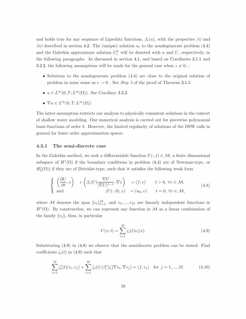
and holds true for any sequence of Lipschitz functions, βǫ(u), with the properties (i) and

(ii) described in section 4.2. The (unique) solution uǫ to the nondegenerate problem (4.4)

and the Galerkin approximate solution Uhǫ will be denoted with u and U , respectively, in

the following paragraphs. As discussed in section 4.1, and based on Corollaries 3.1.1 and

3.2.2, the following assumptions will be made for the general case when z 6= 0, :

• Solutions to the nondegenerate problem (4.4) are close to the original solution of

problem in some sense as ǫ→ 0 . See Step 5 of the proof of Theorem 3.1.1.

• u ∈ L∞(0, T ;L∞(Ω)). See Corollary 3.2.2.

• ∇u ∈ L∞(0, T ;L∞(Ω))

The latter assumption restricts our analysis to physically consistent solutions in the context

of shallow water modeling. Our numerical analysis is carried out for piecewise polynomial

basis functions of order k. However, the limited regularity of solutions of the DSW calls in

general for lower order approximation spaces.

4.3.1 The semi-discrete case

In the Galerkin method, we seek a differentiable function U(·, t) ∈ M, a finite dimensional

subspace of H1(Ω) if the boundary conditions in problem (4.4) are of Newman-type, or

H10 (Ω)) if they are of Dirichlet-type, such that it satisfies the following weak form

(∂U

∂t, v

)+

(βǫ(U)

∇U|∇U |1−γ

,∇v)

= (f, v) t > 0, ∀v ∈ M,

and (U(·, 0), v) = (u0, v) t = 0, ∀v ∈ M,

(4.8)

where M denotes the span viMi=1, and v1, ..., vM are linearly independent functions in

H1(Ω). By construction, we can represent any function in M as a linear combination of

the family vi, thus, in particular

U(x, t) =M∑

i=1

ζi(t)vi(x). (4.9)

Substituting (4.9) in (4.8) we observe that the semidiscrete problem can be stated: Find

coefficients ζi(t) in (4.9) such that

M∑

i=1

ζ ′i(t)(vi, vj) +

M∑

i=1

ζi(t) (β∗ǫ (ζ)∇vi,∇vj) = (f, vj) for j = 1, ...,M. (4.10)

58

with

M∑

i=1

ζi(0)(vi, vj) = (u0, vj), and

β∗ǫ (ζ) := βǫ

(M∑

i=1

ζi(t)vi(x)

) (M∑

i=1

[ζi(t)∇vi(x)]2

) γ−12

. (4.11)

Equivalently, we can express the previous problem as the initial value problem for the system

of nonlinear ordinary differential equations given by

Gζ ′(t) = −B(ζ)ζ + F,

Gζ(0) = b,(4.12)

where the entries of the matrix G = (Gij) are given by Gij = (vi, vj), the entries of the

matrix B(ζ) = (Bij(ζ)) are given by

Bij(ζ) = (β∗ǫ (ζ)∇vi,∇vj), (4.13)

the components of the vectors b = (bj) and F = (Fj) are given by bj = (u0, vj) and

Fj = (f, vj) respectively, and the vector of unknowns is ζ(t) = (ζj(t)).

Whenever U(x, t) given by (4.9) exists, it is called the continuous in time Galerkin approx-

imation or semi-discrete approximation to the weak solution of problem (4.4). Though this

approximation is never computed in practice, it is easy to understand and gives us insight

in our method development. For computational purposes, the variable t is discretized and a

fully algebraic nonlinear system of equations needs to be solved at each time step, in order

to obtain a fully discrete approximation to the solution. This is studied in section 4.3.4.

4.3.2 Existence of the continuous in time Galerkin approximation

Theorem 4.3.1. There exists at least one solution to problem (4.12).

Proof. Since the family vi is linearly independent, the mass matrix G is a Gram matrix,

and thus in particular it is a positive definite and invertible matrix. Hence, problem (4.12)

can be written as: ζ ′(t) = −G−1B(ζ)ζ +G−1F,

ζ(0) = G−1b.(4.14)

Note that the mapping Θ(ζ) : RM → R

M defined by Θ(ζ) = −G−1B(ζ)ζ+G−1F is γ-Holder

continuous and thus, by Peano’s existence theorem for ordinary differential equations (See

59

[43] pp. 10), there exists at least one solution to problem (4.14). Which immediately implies

the statement of the Theorem.

Remark 4.3.1. The fact that Θ(ζ) is γ-Holder continuous is a consequence of B(ζ)ζ being

γ-Holder continuous itself. This can be easily verified recalling definition (4.13). Indeed, if

we let Y = ∇U , the diffusion operator βǫ(U)Y |Y |γ−1 is Lipschitz continuous with respect

to U and γ-Holder continuous w.r.t. Y . Since U and Y depend linearly on ζ, the diffusion

operator will be γ-Holder continuous w.r.t. ζ, and thus the discrete diffusion operator

defined by (4.13) will inherit this property. See Lemma A.0.2 in Appendix A.

4.3.3 Continuous in time a priori error estimate

In this section we will study how close (possibly nonunique) solutions to the continuous

in time Galerkin approximation problem (4.12), U , are to the true weak solution u of

problem (4.4). We focus the analysis to the case when ∇u ∈ L∞(0, T, L∞(Ω)). In the

following paragraphs we will assume that there exists a function u called the interpolant of

u, provided u belongs to some Banach space with certain regularity. The interpolant could

be for example the L2 projection as defined in Lemma 2.4.1. Further assumptions include

that βǫ(u), βǫ(U),∇u,∇U ∈ L∞(0, T, L∞(Ω)). See Remark 4.3.2 below. The error between

solutions of problem (4.12) and the solution of problem (4.4), ‖u− U‖L2 , will be shown to

be bounded by terms that only involve approximation errors between the interpolant and

the true solution of problem (4.4), ‖u − u‖L2 . Thus, reducing the global problem to well

known results in interpolation theory in Hilbert spaces, such as those presented in section

2.4. To simplify the notation in the analysis we will denote with β(x) any element of the

sequence βǫ(x) as described in section 4.2.

Remark 4.3.2. The fact that βǫ(u),∇u ∈ L∞(0, T, L∞(Ω)), for particular finite element

approximation spaces, is a direct consequence of the assumptions that ∇u ∈ L∞(0, T, L∞(Ω)),

(u − z) ∈ L∞(0, T, L∞(Ω)), and Theorem 4.8.7 in [18]. We will further show that, pro-

vided (u − z) ≤ K1 and ∇u ≤ K2 for some (possibly large) constants K1,K2 > 0, then

(U − z) ≤ K1(1 + ǫk1) and ∇U ≤ K2(1 + ǫk2), for small parameters ǫk1 and ǫk2 , and for

particular finite element approximation spaces. See Lemmas 4.3.1 and 4.3.2 below.

Theorem 4.3.2. Let u ∈ W 1,∞(Ω) for all t ∈ [0, T ] be the solution of problem (4.4) and

let U be a solution of problem (4.12). Let χ = u − u be the approximation error between

the interpolant and the true solution of problem (2.1). Further, assume that ∇u,∇U ∈

60

L∞(0, T, L∞(Ω)). Then for all t ∈ [0, T ]

‖u−U‖2L2(Ω) + ‖∇u−∇U‖2

L2(0,T,L2(Ω)) ≤ ‖χ(t)‖2H1(Ω) +C

(‖b− u0‖2

L2(Ω) + ‖χ(0)‖2L2(Ω)+

+

∫ T

0‖χt‖2

L2(Ω) +

∫ T

0‖χ‖2

L2(Ω) +

∫ T

0

∫

Ω|∇χ|2γ

)(4.15)

Proof. Note that a weak solution u of problem (4.4) satisfies the weak form given by (4.8).

Thus, in particular, the following holds

(∂u

∂t, v

)+

(β(U)

∇u|∇u|1−γ

,∇v)

= (f, v) −(∂(u− u)

∂t, v

)+

+

(β(u)

( ∇u|∇u|1−γ

− ∇u|∇u|1−γ

),∇v

)+

((β(U) − β(u))

∇u|∇u|1−γ

,∇v)

(4.16)

Subtracting (4.16) from (4.8) we obtain that

(∂(U − u)

∂t, v

)+

(β(U)

( ∇U|∇U |1−γ

− ∇u|∇u|1−γ

),∇v

)=

(∂(u− u)

∂t, v

)+

+

(β(u)

( ∇u|∇u|1−γ

− ∇u|∇u|1−γ

),∇v

)+

((β(u) − β(U))

∇u|∇u|1−γ

,∇v)

(4.17)

Let ξ = U − u and χ = u− u. Set v = ξ in the previous expression to find

(∂ξ

∂t, ξ

)+

(β(U)

( ∇U|∇U |1−γ

− ∇u|∇u|1−γ

),∇ξ

)=

(∂χ

∂t, ξ

)+

+

(β(u)

( ∇u|∇u|1−γ

− ∇u|∇u|1−γ

),∇ξ

)+

((β(u) − β(U))

∇u|∇u|1−γ

,∇ξ)

(4.18)

The above expression and estimate (4.6) lead to the following inequality

1

2

∂

∂t‖ξ‖2

L2(Ω) + γǫA‖∇ξ‖2L2(Ω) ≤

(∂χ

∂t, ξ

)+

(β(u)

( ∇u|∇u|1−γ

− ∇u|∇u|1−γ

),∇ξ

)

+

((β(u) − β(U))

∇u|∇u|1−γ

,∇ξ), (4.19)

where1 A := inf(0,T )×Ω

(A0) = inf(0,T )×Ω

1/(‖∇U‖L∞(0,T,L∞(Ω)) + ‖∇u‖L∞(0,T,L∞(Ω)))

)1−γ.

The terms on the right hand side can be bounded in the following way. The first one, using

1See remark 4.3.3

61

Young’s inequality: ∣∣∣∣

∫

Ω

∂χ

∂tξ

∣∣∣∣ ≤1

2

(‖χt‖2

L2(Ω) + ‖ξ‖2L2(Ω)

). (4.20)

The second one, using estimate (4.7) and Young’s inequality with ǫ1:

∣∣∣∣

∫

Ωβ(u)

( ∇u|∇u|1−γ

− ∇u|∇u|1−γ

)∇ξ

∣∣∣∣ ≤ 2

γM

∫

Ω|∇χ|γ |∇ξ| (4.21)

≤ 2

γM

(1

2ǫ1

∫

Ω|∇χ|2γ +

ǫ12‖∇ξ‖2

L2(Ω)

)

(4.22)

whereM = ‖β(u)‖L∞(Ω). The third one, using estimate (4.5), Cauchy-Schwarz, and Young’s

inequalities with ǫ2

∣∣∣∣∫

Ω(β(u) − β(U))

∇u|∇u|1−γ

∇ξ∣∣∣∣ ≤ M∗

∫

Ω|u− U ||∇u|γ |∇ξ| (4.23)

≤ M∗‖∇u‖γL∞(Ω)‖u− U‖L2(Ω)‖∇ξ‖L2(Ω)

≤ M∗‖∇u‖γL∞(Ω)

(1

2ǫ2(‖χ‖2

L2(Ω) + ‖ξ‖2L2(Ω)) +

ǫ22‖∇ξ‖2

L2(Ω)

),

where M∗ = α max(‖β(u)‖L∞(Ω), ‖β(U)‖L∞(Ω))α−1.

From estimate (4.6), provided ∇u,∇U ∈ L∞(0, T, L∞(Ω)), there exists a constant ǫ3 > 0

such that

γǫA ≥ ǫ3 for all t ∈ [0, T ] (4.24)

we can combine expressions (4.19)-(4.23) and choose ǫ1 and ǫ2 small enough to obtain that

for some ǫ > 0 and some constants Ci > 0 (1 ≤ i ≤ 4)

1

2

∂

∂t‖ξ‖2

L2(Ω) + ǫ‖∇ξ‖2L2(Ω) ≤ C1‖ξ‖2

L2(Ω) +C2‖χt‖2L2(Ω) +C3‖χ‖2

L2(Ω) +C4

∫

Ω|∇χ|2γ (4.25)

Since the second term on the left hand side is nonnegative, we can use Gronwall’s Lemma

in the previous expression to obtain that for all t ∈ [0, T ]

‖ξ(t)‖2L2(Ω) ≤ C5(T )

(‖ξ(0)‖2

L2(Ω) + C2

∫ T

0‖χt‖2

L2(Ω) + C3

∫ T

0‖χ‖2

L2(Ω) + C4

∫ T

0

∫

Ω|∇χ|2γ

).

(4.26)

Observe that

‖u− U‖2L2(Ω) ≤ ‖U − u‖2

L2(Ω) + ‖u− u‖2L2(Ω) = ‖ξ(t)‖2

L2(Ω) + ‖χ(t)‖2L2(Ω). (4.27)

62

and

‖ξ(0)‖2L2(Ω) = ‖b− u0‖2

L2(Ω) ≤ ‖b− u0‖2L2(Ω) + ‖u0 − u0‖2

L2(Ω)

≤ ‖b− u0‖2L2(Ω) + ‖χ(0)‖2

L2(Ω) (4.28)

Thus, combining result (4.26), the two previous expressions and letting C = max(C5Ci) for

i = 2, 3, 4. we can establish the first portion of the statement of the Theorem (4.15).

In order to complete the proof we need to find a bound for the gradients. This is done

integrating expression (4.25) in time. Note that on the left hand side we have

1

2‖ξ(T )‖2

L2(Ω) −1

2‖ξ(0)‖2

L2(Ω) + ǫ‖∇u−∇U‖2L2(0,T,L2(Ω)). (4.29)

Since the first term is nonnegative, the following holds from the time integration of (4.25)

‖∇ξ‖2L2(0,T,L2(Ω)) ≤ C

(1

2‖ξ(0)‖2

L2(Ω) +

∫ T

0‖ξ‖2

L2(Ω) +

∫ T

0‖χt‖2

L2(Ω) +

∫ T

0‖χ‖2

L2(Ω)+

+

∫ T

0

∫

Ω|∇χ|2γ

). (4.30)

Estimate (4.15) follows from the observation that

‖∇u−∇U‖2L2(0,T,L2(Ω)) ≤ ‖∇U −∇u‖2

L2(0,T,L2(Ω)) + ‖∇u−∇u‖2L2(0,T,L2(Ω))

≤ ‖∇ξ(t)‖2L2(0,T,L2(Ω)) + ‖∇χ(t)‖2

L2(0,T,L2(Ω)).

and the combination of (4.26) and (4.30). This concludes the proof.

Remark 4.3.3. Note that the error estimate collapses if condition (4.24) is not satisfied.

This is the reason why we need to use both: the family of nondegenerate βǫ(x) > ǫ, and the

assumptions that ∇u ∈ L∞(0, T, L∞(Ω)) and ∇U ∈ L∞(0, T, L∞(Ω)). The latter assump-

tions ensure that A > 0 since ∇u ∈ L∞(0, T, L∞(Ω)) implies that ∇u ∈ L∞(0, T, L∞(Ω))

for an appropriate finite element space.

Corollary 4.3.1 (Stability). Under the conditions of Theorem 4.3.2, the method is stable.

Proof. Write U(t) = U(t) − u(t) + u(t) and use the triangle inequality to find

‖U(t)‖L2(Ω) ≤ ‖U(t) − u(t)‖L2(Ω) + ‖u(t)‖L2(Ω)

Using the previous theorem and assuming that u ∈ L2(Ω) the result is immediate.

63

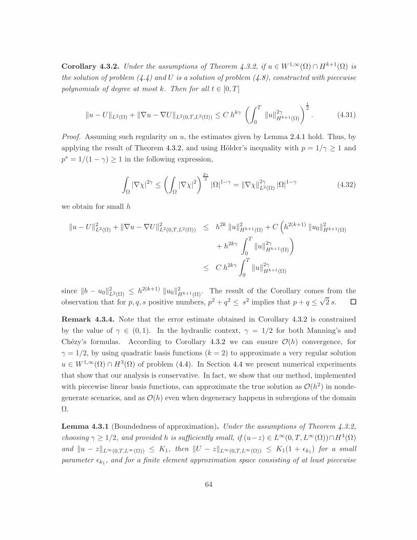
Corollary 4.3.2. Under the assumptions of Theorem 4.3.2, if u ∈W 1,∞(Ω) ∩Hk+1(Ω) is

the solution of problem (4.4) and U is a solution of problem (4.8), constructed with piecewise

polynomials of degree at most k. Then for all t ∈ [0, T ]

‖u− U‖L2(Ω) + ‖∇u−∇U‖L2(0,T,L2(Ω)) ≤ C hkγ

(∫ T

0‖u‖2γ

Hk+1(Ω)

) 12

. (4.31)

Proof. Assuming such regularity on u, the estimates given by Lemma 2.4.1 hold. Thus, by

applying the result of Theorem 4.3.2, and using Holder’s inequality with p = 1/γ ≥ 1 and

p∗ = 1/(1 − γ) ≥ 1 in the following expression,

∫

Ω|∇χ|2γ ≤

(∫

Ω|∇χ|2

) 2γ2

|Ω|1−γ = ‖∇χ‖2γL2(Ω)

|Ω|1−γ (4.32)

we obtain for small h

‖u− U‖2L2(Ω) + ‖∇u−∇U‖2

L2(0,T,L2(Ω)) ≤ h2k ‖u‖2Hk+1(Ω) + C

(h2(k+1) ‖u0‖2

Hk+1(Ω)

+ h2kγ

∫ T

0‖u‖2γ

Hk+1(Ω)

)

≤ C h2kγ

∫ T

0‖u‖2γ

Hk+1(Ω)

since ‖b − u0‖2L2(Ω) ≤ h2(k+1) ‖u0‖2

Hk+1(Ω). The result of the Corollary comes from the

observation that for p, q, s positive numbers, p2 + q2 ≤ s2 implies that p+ q ≤√

2 s.

Remark 4.3.4. Note that the error estimate obtained in Corollary 4.3.2 is constrained

by the value of γ ∈ (0, 1). In the hydraulic context, γ = 1/2 for both Manning’s and

Chezy’s formulas. According to Corollary 4.3.2 we can ensure O(h) convergence, for

γ = 1/2, by using quadratic basis functions (k = 2) to approximate a very regular solution

u ∈ W 1,∞(Ω) ∩H3(Ω) of problem (4.4). In Section 4.4 we present numerical experiments

that show that our analysis is conservative. In fact, we show that our method, implemented

with piecewise linear basis functions, can approximate the true solution as O(h2) in nonde-

generate scenarios, and as O(h) even when degeneracy happens in subregions of the domain

Ω.

Lemma 4.3.1 (Boundedness of approximation). Under the assumptions of Theorem 4.3.2,

choosing γ ≥ 1/2, and provided h is sufficiently small, if (u−z) ∈ L∞(0, T, L∞(Ω))∩H4(Ω)

and ‖u − z‖L∞(0,T,L∞(Ω)) ≤ K1, then ‖U − z‖L∞(0,T,L∞(Ω)) ≤ K1(1 + ǫk1) for a small

parameter ǫk1, and for a finite element approximation space consisting of at least piecewise

64

cubic basis functions.

Proof. Write (U − z) as (U − u+ u− z) to find

‖U − z‖L∞(0,T,L∞(Ω)) ≤ ‖U − u‖L∞(0,T,L∞(Ω)) + ‖u− z‖L∞(0,T,L∞(Ω)). (4.33)

Choose u as in the definition (2.8), and choose at least M = P3 (piecewise cubic basis

functions, k = 3). The fact that the interpolant (u − z) ∈ L∞(0, T, L∞(Ω)) provided

(u− z) ∈ L∞(0, T, L∞(Ω)) ∩H4(Ω), for a bounded and smooth time independent function

z, is a consequence of Theorem 4.8.7 in [18]. Thus, ‖u−z‖L∞(0,T,L∞(Ω)) ≤ K1 for sufficiently

small h. Now, from Corollary 4.3.2 and Lemma 2.4.2 we obtain

‖U − z‖L∞(0,T,L∞(Ω)) ≤ ‖U − u‖L∞(0,T,L∞(Ω)) +K1

≤ K0 h−1‖U − u‖L∞(0,T,L2(Ω)) +K1

≤ K0 h3γ−1

(∫ T

0‖u‖2γ

H4(Ω)

) 12

+K1

Thus, we can choose a sufficiently small h so that K0 h1/2(∫ T

0 ‖u‖2γH4(Ω)

) 12 ≤ ǫk1K1, which

implies

‖U − z‖L∞(0,T,L∞(Ω)) ≤ K1(1 + ǫk1)

This establishes the result of the Lemma.

Lemma 4.3.2 (Boundedness of the gradient of the approximation). Under the assump-

tions of Theorem 4.3.2, choosing γ ≥ 1/2, and provided h is sufficiently small, if u ∈L∞(0, T, L∞(Ω)) ∩ H5(Ω), ∇u ∈ L∞(0, T, L∞(Ω)) and ‖∇u‖L∞(0,T,L∞(Ω)) ≤ K2 , then

‖∇U‖L∞(0,T,L∞(Ω)) ≤ K2(1 + ǫk2) for a finite element approximation space consisting of at

least fourth degree piecewise polynomial basis functions.

Proof. Similar to the one in Lemma (4.3.1).

4.3.4 Fully discrete approximation

In this section we will further proceed to consider discretization with respect to time. We

will denote by dt the time step and with Un the approximation of u(t) at time t = tn = ndt.

In order to write down the method we will replace the time derivative in (4.8) by the quotient

δUn =Un − Un−1

dt, (4.34)

65

to obtain the following Backward Euler scheme

(δUn, v) +

(βǫ(U

n)

|∇Un|1−γ∇Un,∇v

)= (fn, v) n dt ∈ [0, T ], ∀v ∈ M,

and (U0, v) = (u0, v) ∀v ∈ M.

(4.35)

The previous expression defines Un implicitly for Un−1 given and it can be written as follows

(Un, v) + dt

(βǫ(U

n)

|∇Un|1−γ∇Un,∇v

)= (Un−1 + dt fn, v) ∀v ∈ M, (4.36)

or in matrix form, using the definitions explained in section 4.3.1,

(G+ dt B(ζn))ζn = Gζn−1 + dt F (tn), (4.37)

where fn (alt. F (tn)) is a known function (alt. matrix)

4.3.4.1 Fully discrete A priori error estimate

In this section we will study how close solutions to the fully discrete Galerkin approximation

problem (4.35) are to the true weak solution of problem (2.1). The proof follows immedi-

ately from the semi-discrete estimates and it is presented for completeness. Once more, in

the analysis we will denote with β(x) any element of the sequence βǫ(x) as described in

section 4.2.

Theorem 4.3.3. Let u ∈ W 1,∞(Ω) for all t ∈ [0, T ] be the solution of problem (4.4) and

let Un be a solution of problem (4.35) at tn = n dt. Let also χn = u(tn) − u(tn) be the

approximation error between the interpolant and the true solution of problem (2.1). Then

for all tn ∈ [0, T ]

‖u(tn) − Un‖2L2(Ω) + dt

n∑

j=1

‖∇u(tj) −∇U j‖2L2(Ω) ≤ C‖b− u0‖2

L2(Ω) + ‖χ0‖2L2(Ω)+

+ dt C

n∑

j=1

(‖ut(tj) − δu(tj)‖2

L2(Ω) + ‖χj‖2L2(Ω) +

∫

Ω

∣∣∇χj∣∣2γ)

(4.38)

Proof. Observe that identifying un = u(tn) and un = u(tn) a similar calculation to (4.17)

66

yields

(δ(Un − un), v) +

(β(Un)

( ∇Un

|∇Un|1−γ− ∇un

|∇un|1−γ

),∇v

)= (un

t − δun, v) +

+

(β(un)

( ∇un

|∇un|1−γ− ∇un

|∇un|1−γ

),∇v

)+

((β(un) − β(Un))

∇un

|∇un|1−γ,∇v

)(4.39)

Now, let ξn = Un− u(tn) and χn = u(tn)− u(tn) and choose v = ξn. Using estimates (4.21)

and (4.23) we obtain

(δξn, ξn)+γ(β(Un))A‖∇ξn‖2L2(Ω) ≤ (un

t − δun, ξn)+1

ǫ2C‖ξn‖2

L2(Ω)+C(ǫ2+ǫ1)‖∇ξn‖2L2(Ω)+

+1

2ǫ2‖χn‖2

L2(Ω) +1

2ǫ1C

∫

Ω|∇χn|2γ . (4.40)

If condition (4.24) is satisfied, then for ǫ1 and ǫ2 small enough, the previous expression

implies

‖ξn‖2L2(Ω) ≤ (ξn−1, ξn)+dt (un

t − δun, ξn)+dtC‖ξn‖2L2(Ω)+dtC‖χn‖2

L2(Ω)+dtC

∫

Ω|∇χn|2γ ,

(4.41)

which yields

(1− dt C)‖ξn‖2L2(Ω) ≤ ‖ξn−1‖2

L2(Ω) + dt ‖unt − δun‖2

L2(Ω) + dt C‖χn‖2L2(Ω) + dt C

∫

Ω|∇χn|2γ .

(4.42)

Using the Taylor expansion for (1 − dt C)−1 around zero we can rewrite the previous ex-

pression for small dt:

‖ξn‖2L2(Ω) ≤ (1 + dt C)‖ξn−1‖2

L2(Ω) + dt C Rn (4.43)

where

Rn = ‖unt − δun‖2

L2(Ω) + ‖χn‖2L2(Ω) +

∫

Ω|∇χn|2γ

Making use of inequality (4.43) repeatedly we find that

‖ξn‖2L2(Ω) ≤ (1 + dt C)n‖ξ0‖2

L2(Ω) + dt C

n∑

j=1

(1 + dt C)n−jRj

≤ C‖ξ0‖2L2(Ω) + dt C

n∑

j=1

Rj for tn = dt n ∈ [0, T ] (4.44)

67

which together with

‖ξ0‖2L2(Ω) = ‖b− u0‖2

L2(Ω) ≤ ‖b− u0‖2L2(Ω) + ‖u0 − u0‖2

L2(Ω)

≤ ‖b− u0‖2L2(Ω) + ‖χ0‖2

L2(Ω)

establish the first portion of the statement of the Theorem. In order to find the appropriate

estimate on the gradients a similar argument to the one in the proof of the continuous

in time a priori error estimate has to be used. Both estimates lead to the result of the

Theorem.

Corollary 4.3.3. If u ∈W 1,∞(Ω) ∩Hk+1(Ω) is the solution of problem (4.4) and Un is a

solution of problem (4.35) at tn = n dt, constructed with piecewise polynomials of degree at

most k. Then for all tn ∈ [0, T ]

‖u(tn) − Un‖L2(Ω) + dt∑

n

‖∇u(tn) −∇Un‖L2(Ω) ≤ C(u, tn) (dt + hkγ) (4.45)

Proof. Given the regularity of u, the quantity Rj can be bounded using the estimates given

by Lemma 2.4.1, the fact that ‖unt − δun‖2

L2(Ω) ≤ C∗(u)dt2 (see [60]), and applying the

results of Theorem 4.3.3. Thus,

‖u(tn) − Un‖2L2(Ω) + dt

∑

n

‖∇u(tn) −∇Un‖2L2(Ω) ≤ C‖b− u0‖2

L2(Ω) + h2(k+1) ‖u0‖2Hk+1(Ω) +

dt Cn∑

j=1

(C∗(u)dt2 + h2k ‖u(tn)‖2

Hk+1(Ω)+

+ h2kγ ‖u(tn)‖2γHk+1(Ω)

)

≤ C(u, tn) (dt + hkγ)2. (4.46)

Recall that for p, q, s positive numbers, p2 + q2 ≤ s2 implies that p + q ≤√

2 s. Thus, the

result of the Corollary follows immediately.

4.4 Numerical Experiments. 1D

A lumped mass continuous Galerkin code with piecewise linear basis functions was imple-

mented in order to perform numerical experiments aimed at investigating: (i) The accuracy

and validity of the numerical method previously described to solve the DSW equation for

the case when z = 0, see section 4.4.1, (ii) the applicability of the DSW equation as a

68

model to simulate observed quantities (such as water discharge and depth profile) in an

experimental setting for a prescribed bathymetry z = z(x) 6= 0, see section 4.4.2, and (iii)

the qualitative properties of solutions to the DSW in its general form (2.1).

Even though Lemmas 4.3.1 and 4.3.2 suggest that one should use at least fourth order poly-

nomial basis functions in order to ensure the boundedness of both U − z and ∇U and thus

convergence of the numerical scheme, in practice, we found that the use of piecewise lin-

ear basis functions was appropriate. Furthermore, our numerical experiments showed that

the implementation of the regularizing Lipschitz functional βǫ(u) > ǫ (instead of u − z),

as described in section 4.2, was not necessary. In fact, we found that the stability of the

code behaved similarly with or without the implementation of the βǫ(u) > 0, and generally

‖Uǫ − U‖L2(Ω) ∽ O(ǫ), with Uǫ the numerical solution of the nondegenerate problem (4.4),

and U the numerical solution of the possibly degenerate problem (2.1).

A lumped mass approach was chosen since for well behaved nonlinear parabolic equations

such schemes satisfy a maximum principle and thus provide a monotone and physically

consistent way to approach the solution, see [60]. For computational purposes, problem

(4.37) was approximated by the semi-implicit scheme

(G+ dt B(ζ(l)))ζn = Gζn−1 + dt F (tn). (4.47)

A Picard Iteration approach

ζ(l) = (G+ dt B(ζ(l−1)))−1(Gζn−1 + dt F (tn)),

with an initial guess ζ(0) = ζn−1 was used in order to resolve the nonlinearity, with the

assumption that

liml→∞

(G+ dt B(ζ(l))) = (G+ dt B(ζn)). (4.48)

In practice, the iteration process was stopped when ‖ζ(l) − ζ(l−1)‖2l2(Ω) ≤ τ for a prescribed

tolerance τ , and ζn was set equal to the value of ζ(l) in the last iteration. In all our

experiments we chose α = 5/3 and γ = 1/2 (as in [73] and [38]). These values correspond

to Manning’s formula. Numerical studies addressing the case when z = 0, α ≥ 1 and γ = 1,

which corresponds to the Porous Medium Equation, include for example: [53] and [72].

4.4.1 Convergence analysis

As suggested in the previous sections, convergence of the numerical method proposed to

approximate the DSW equation may fail if the depth u − z is zero or if its gradient ∇u

69

−6 −4 −2 0 2 4 60

0.5

1

1.5

2

2.5Barenblatt solutions

t=.1t=.5t=1t=1.5t=2t=2.5

−6 −4 −2 0 2 4 60

0.5

1

1.5

2

2.5Analytical vs numerical Barenblatt solutions.

Num. approx. t=.1

Num. approx. t=.5

Num. approx. t=1

Num. approx. t=1.5

Num. approx. t=2

Num. approx. t=2.5

True soln. t=.1

True soln. t=.5

True soln. t=1

True soln. t=1.5

True soln. t=2

True soln. t=2.5

Figure 4.1: Comparison of numerically simulated compactly supported solutions for α =5/3 and γ = 1/2. (Left) Analytical Barenblatt solutions (z = 0), (Right) Numerical vsanalytical solutions (z = 0).

is unbounded. In order to investigate the accuracy and validity of the numerical method

in different circumstances we chose two approaches: the first one consisted of reproducing

a Lipschitz continuous compactly supported solution of (2.1) presented in [35] for the 1-

dimensional case, for z = 0, f = 0, and Ω = R. The second one consisted of choosing

a simple function u(x, t) ≥ 0 with unbounded gradient at x = 0 that we used to create

a right hand side f(x, t). This was done by applying the differential operator defined by

the left hand side of (2.1). We then used our method to approximate this u. For both

cases we obtained convergence rates for a variety of scenarios and present them in the next

paragraphs.

Remark 4.4.1. Despite the fact that Corollary 4.3.3 would only ensure convergence results

of the type, ‖u(tn) − Un‖L2(Ω) ≤ C(u, tn) (dt + h1/2) for γ = 1/2, and nondegenerate

solutions u ∈ H2(Ω) using piecewise linear basis functions (k = 1), we chose the time

step comparable to or smaller than the square of the grid diameter, dt . h2 = dx2, in

our convergence experiments. This was done in order to investigate if optimality in the

convergence rates (i.e. ‖u(tn) − Un‖L2(Ω) ≤ C(u, tn) (dt + h2)) could be achieved for say,

nondegenerate solutions with bounded gradients. Intuitively, under these conditions, (2.1)

should resemble a well behaved nonlinear parabolic problem.

4.4.1.1 Compactly supported solution

Most of the Barenblatt solutions presented in this subsection do not exhibit the properties

of solutions assumed in order to derive the DSW equation from the SWE (such as the fact

70

that the gradient of the solution be comparable to the gradient of the bathymetry) and thus

they would be incorrect models for shallow water flows. However, from the numerical point

of view, having an analytic expression of the solution makes the convergence analysis much

simpler. The explicit expression of a Barenblatt solution for (2.1) is presented in [35] and

given by

u(x, t) = t− 1

γ(m+1)

[C − k(m,γ) |Φ|

γ+1γ

] γmγ−1

+(4.49)

where [s(x)]+ denotes the positive part of s(x), m = 1+α/γ, C is a positive function related

to the initial mass M , given by

M =

∫ ∞

−∞u(x, t)dx,

and

k(m,γ) =mγ − 1

m(γ + 1)

(1

γ(m+ 1)

) 1γ

, and Φ = x t− 1

γ(m+1)

The function given by (4.49) is Lipschitz continuous and compactly supported, thus it is

almost everywhere differentiable and its gradient is bounded wherever it exists. By changing

the numerical domain Ω we managed to verify how the numerical method approximates the

solution both when it is globally not degenerate, u > 0, and when it degenerates in some

subsets of Ω. For our calculations in the degenerate case, we chose a numerical interval

[−L,L] big enough so that the free boundary would always be inside the domain Ω for

t ∈ [t0, tf ]. The results are shown in Table 4.1(a) for the nondegenerate case, and in Table

4.1(b) for the degenerate case. In all cases t0 = 2 and tf = 2.1 and the Picard Iteration

scheme was run until the tolerance value met the condition τ ≤ 10−10. We computed the

numerical solutions and compared them to the true solution using dt = 1/10 and dx = 1/20

to produce the plots in Figure 4.1. The computed mass M of the numerical solution was

calculated as a function of time t and it was observed to be close to the constant M = 5.8465

which corresponds to the value of the mass of the true solution (4.49) in the time interval

t ∈ [.1, 2.5].

4.4.1.2 Artificial right hand side

The function u(x, t) ≥ 0 with unbounded gradient at x = 0 that we used to create a right

hand side f(x, t) by applying the differential operator defined by the left hand side of (2.1)

71

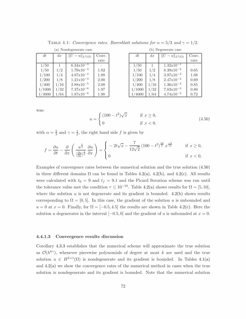
Table 4.1: Convergence rates. Barenblatt solutions for α = 5/3 and γ = 1/2.

(a) Nondegenerate case

dt dx ‖U − u‖L2(Ω) Conv.rate

1/50 1 6.34x10−3 ·1/50 1/2 1.79x10−3 1.821/100 1/4 4.87x10−4 1.881/200 1/8 1.21x10−4 2.001/400 1/16 2.88x10−5 2.081/1000 1/32 7.37x10−6 1.971/4000 1/64 1.87x10−6 1.98

(b) Degenerate case

dt dx ‖U − u‖L2(Ω) Conv.rate

1/50 1 1.32x10−1 ·1/50 1/2 8.39x10−2 0.651/100 1/4 3.97x10−2 1.081/200 1/8 2.47x10−2 0.691/400 1/16 1.36x10−2 0.851/1000 1/32 7.83x10−3 0.801/4000 1/64 4.74x10−3 0.72

was:

u =

(100 − t2)

√x if x ≥ 0,

0 if x < 0.(4.50)

with α = 53 and γ = 1

2 , the right hand side f is given by

f =∂u

∂t− ∂

∂x

(u

53

|∂u∂x |

12

∂u

∂x

)

=

− 2t√x− 7

12√

2(100 − t2)

136 x

−512 if x ≥ 0,

0 if x < 0,

Examples of convergence rates between the numerical solution and the true solution (4.50)

in three different domains Ω can be found in Tables 4.2(a), 4.2(b), and 4.2(c). All results

were calculated with t0 = 9 and tf = 9.1 and the Picard Iteration scheme was run until

the tolerance value met the condition τ ≤ 10−10. Table 4.2(a) shows results for Ω = [5, 10],

where the solution u is not degenerate and its gradient is bounded. 4.2(b) shows results

corresponding to Ω = [0, 5]. In this case, the gradient of the solution u is unbounded and

u = 0 at x = 0. Finally, for Ω = [−0.5, 4.5] the results are shown in Table 4.2(c). Here the

solution u degenerates in the interval [−0.5, 0] and the gradient of u is unbounded at x = 0.

4.4.1.3 Convergence results discussion

Corollary 4.3.3 establishes that the numerical scheme will approximate the true solution

as O(hkγ), whenever piecewise polynomials of degree at most k are used and the true

solution u ∈ Hk+1(Ω) is nondegenerate and its gradient is bounded. In Tables 4.1(a)

and 4.2(a) we show the convergence rates of the numerical method in cases when the true

solution is nondegenerate and its gradient is bounded. Note that the numerical solution

72

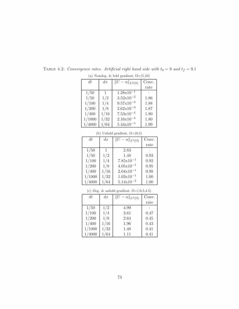
Table 4.2: Convergence rates. Artificial right hand side with t0 = 9 and tf = 9.1

(a) Nondeg. & bdd gradient, Ω=(5,10)

dt dx ‖U − u‖L2(Ω) Conv.

rate

1/50 1 1.28x10−1 ·1/50 1/2 3.52x10−2 1.861/100 1/4 9.57x10−3 1.881/200 1/8 2.62x10−3 1.871/400 1/16 7.53x10−4 1.801/1000 1/32 2.16x10−4 1.801/4000 1/64 5.44x10−5 1.99

(b) Unbdd gradient, Ω=(0,5)

dt dx ‖U − u‖L2(Ω) Conv.

rate

1/50 1 2.83 ·1/50 1/2 1.48 0.931/100 1/4 7.85x10−1 0.921/200 1/8 4.05x10−1 0.951/400 1/16 2.04x10−1 0.981/1000 1/32 1.03x10−1 1.001/4000 1/64 5.14x10−2 1.00

(c) Deg. & unbdd gradient, Ω=(-0.5,4.5)

dt dx ‖U − u‖L2(Ω) Conv.

rate

1/50 1/2 4.99 ·1/100 1/4 3.61 0.471/200 1/8 2.64 0.451/400 1/16 1.96 0.431/1000 1/32 1.48 0.411/4000 1/64 1.11 0.41

73

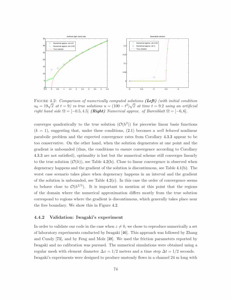
−0.5 0 0.5 1 1.5 2 2.5 3 3.5 4 4.50

5

10

15

20

25

30

35Artificial right−hand side

Numerical approx. dx=1/2

Numerical approx. dx=1/16

True solution

−6 −5.5 −5 −4.5 −4

0

0.05

0.1

0.15

0.2

Barenblatt solution

Numerical approx. dx=1/16

Numerical approx. dx=1

True solution

Figure 4.2: Comparison of numerically computed solutions (Left) (with initial conditionu0 = 19

√x at t = 9) vs true solutions u = (100 − t2)

√x at time t = 9.2 using an artificial

right hand side Ω = [−0.5, 4.5] (Right) Numerical approx. of Barenblatt Ω = [−6, 6].

converges quadratically to the true solution (O(h2)) for piecewise linear basis functions

(k = 1), suggesting that, under these conditions, (2.1) becomes a well behaved nonlinear

parabolic problem and the expected convergence rates from Corollary 4.3.3 appear to be

too conservative. On the other hand, when the solution degenerates at one point and the

gradient is unbounded (thus, the conditions to ensure convergence according to Corollary

4.3.3 are not satisfied), optimality is lost but the numerical scheme still converges linearly

to the true solution (O(h)), see Table 4.2(b). Close to linear convergence is observed when

degeneracy happens and the gradient of the solution is discontinuous, see Table 4.1(b). The

worst case scenario takes place when degeneracy happens in an interval and the gradient

of the solution is unbounded, see Table 4.2(c). In this case the order of convergence seems

to behave close to O(h2/5). It is important to mention at this point that the regions

of the domain where the numerical approximation differs mostly from the true solution

correspond to regions where the gradient is discontinuous, which generally takes place near

the free boundary. We show this in Figure 4.2.

4.4.2 Validation: Iwagaki’s experiment

In order to validate our code in the case when z 6= 0, we chose to reproduce numerically a set

of laboratory experiments conducted by Iwagaki [46]. This approach was followed by Zhang

and Cundy [73], and by Feng and Molz [38]. We used the friction parameters reported by

Iwagaki and no calibration was pursued. The numerical simulations were obtained using a

regular mesh with element diameter ∆x = 1/2 meters and a time step ∆t = 1/2 seconds.

Iwagaki’s experiments were designed to produce unsteady flows in a channel 24 m long with

74

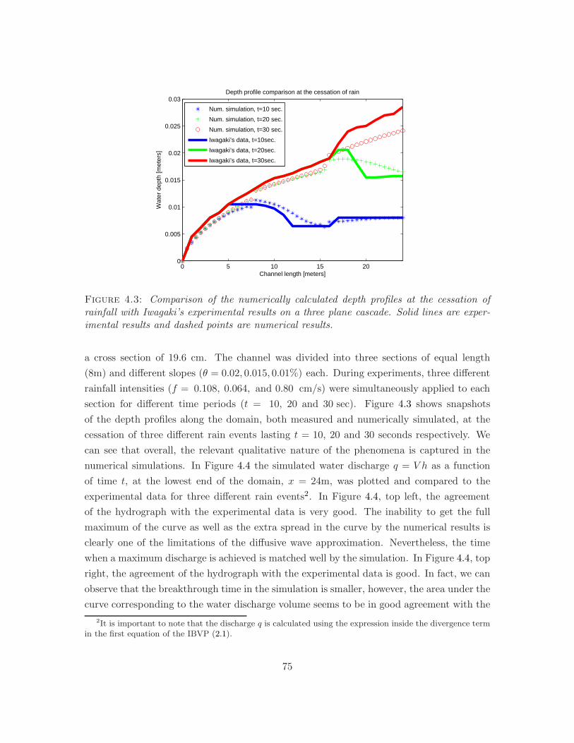
0 5 10 15 200

0.005

0.01

0.015

0.02

0.025

0.03

Channel length [meters]

Wat

er d

epth

[met

ers]

Depth profile comparison at the cessation of rain

Num. simulation, t=10 sec.

Num. simulation, t=20 sec.

Num. simulation, t=30 sec.

Iwagaki’s data, t=10sec.

Iwagaki’s data, t=20sec.

Iwagaki’s data, t=30sec.

Figure 4.3: Comparison of the numerically calculated depth profiles at the cessation ofrainfall with Iwagaki’s experimental results on a three plane cascade. Solid lines are exper-imental results and dashed points are numerical results.

a cross section of 19.6 cm. The channel was divided into three sections of equal length

(8m) and different slopes (θ = 0.02, 0.015, 0.01%) each. During experiments, three different

rainfall intensities (f = 0.108, 0.064, and 0.80 cm/s) were simultaneously applied to each

section for different time periods (t = 10, 20 and 30 sec). Figure 4.3 shows snapshots

of the depth profiles along the domain, both measured and numerically simulated, at the

cessation of three different rain events lasting t = 10, 20 and 30 seconds respectively. We

can see that overall, the relevant qualitative nature of the phenomena is captured in the

numerical simulations. In Figure 4.4 the simulated water discharge q = V h as a function

of time t, at the lowest end of the domain, x = 24m, was plotted and compared to the

experimental data for three different rain events2. In Figure 4.4, top left, the agreement

of the hydrograph with the experimental data is very good. The inability to get the full

maximum of the curve as well as the extra spread in the curve by the numerical results is

clearly one of the limitations of the diffusive wave approximation. Nevertheless, the time

when a maximum discharge is achieved is matched well by the simulation. In Figure 4.4, top

right, the agreement of the hydrograph with the experimental data is good. In fact, we can

observe that the breakthrough time in the simulation is smaller, however, the area under the

curve corresponding to the water discharge volume seems to be in good agreement with the

2It is important to note that the discharge q is calculated using the expression inside the divergence termin the first equation of the IBVP (2.1).

75

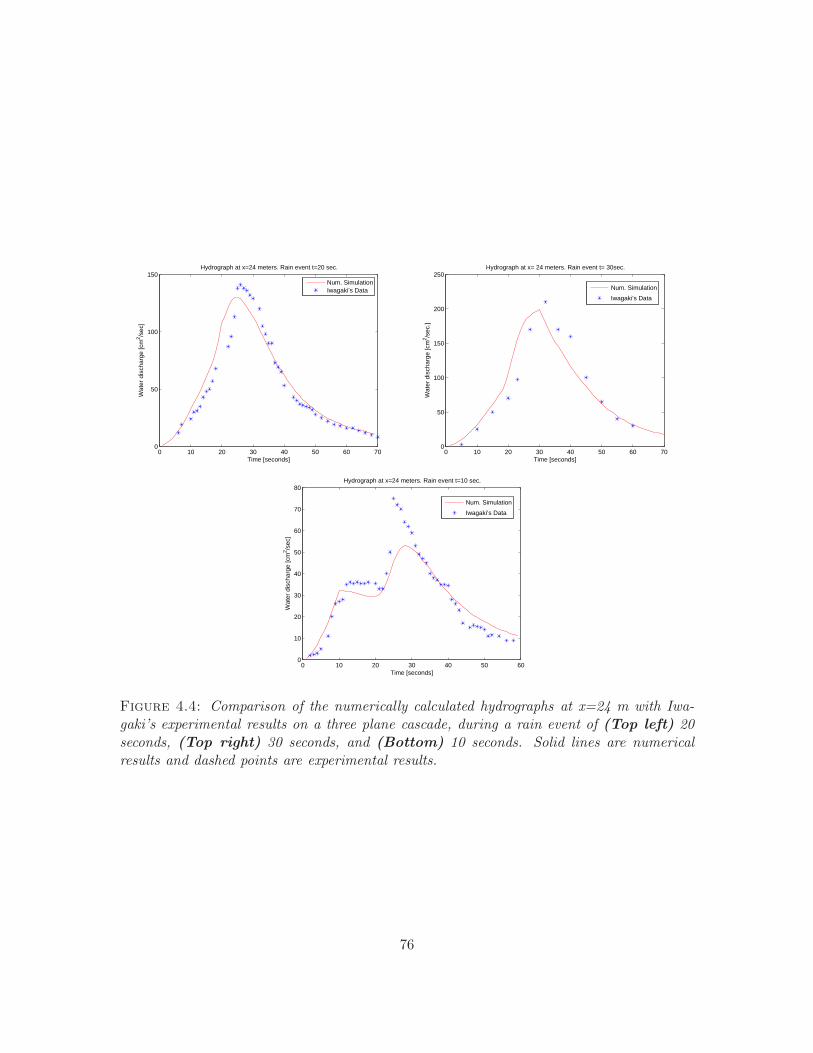
0 10 20 30 40 50 60 700

50

100

150

Time [seconds]

Wat

er d

isch

arge

[cm

2 /sec

]

Hydrograph at x=24 meters. Rain event t=20 sec.

Num. SimulationIwagaki’s Data

0 10 20 30 40 50 60 700

50

100

150

200

250

Time [seconds]

Wat

er d

isch

arge

[cm

2 /sec

.]

Hydrograph at x= 24 meters. Rain event t= 30sec.

Num. Simulation

Iwagaki’s Data

0 10 20 30 40 50 600

10

20

30

40

50

60

70

80

Time [seconds]

Wat

er d

isch

arge

[cm

2 /sec

]

Hydrograph at x=24 meters. Rain event t=10 sec.

Num. Simulation

Iwagaki’s Data

Figure 4.4: Comparison of the numerically calculated hydrographs at x=24 m with Iwa-gaki’s experimental results on a three plane cascade, during a rain event of (Top left) 20seconds, (Top right) 30 seconds, and (Bottom) 10 seconds. Solid lines are numericalresults and dashed points are experimental results.

76

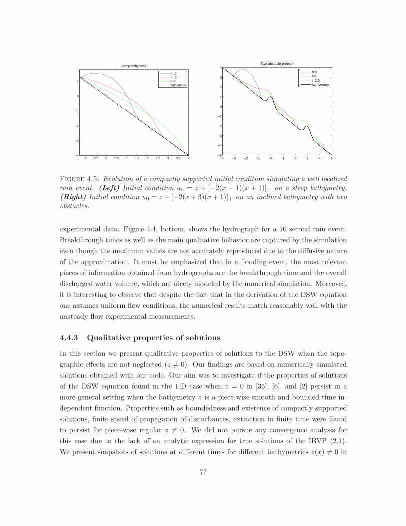
−1 −0.5 0 0.5 1 1.5 2 2.5 3 3.5 4−4

−3

−2

−1

0

1

Steep bathymetry

t= .1t= .5t= 1bathymetry

−4 −3 −2 −1 0 1 2 3 4 5−5

−4

−3

−2

−1

0

1

2

3

4Two obstacle problem

t=0t=1t=2.5bathymetry

Figure 4.5: Evolution of a compactly supported initial condition simulating a well localizedrain event. (Left) Initial condition u0 = z + [−2(x − 1)(x + 1)]+ on a steep bathymetry,(Right) Initial condition u0 = z + [−2(x+ 3)(x+ 1)]+ on an inclined bathymetry with twoobstacles.

experimental data. Figure 4.4, bottom, shows the hydrograph for a 10 second rain event.

Breakthrough times as well as the main qualitative behavior are captured by the simulation

even though the maximum values are not accurately reproduced due to the diffusive nature

of the approximation. It must be emphasized that in a flooding event, the most relevant

pieces of information obtained from hydrographs are the breakthrough time and the overall

discharged water volume, which are nicely modeled by the numerical simulation. Moreover,

it is interesting to observe that despite the fact that in the derivation of the DSW equation

one assumes uniform flow conditions, the numerical results match reasonably well with the

unsteady flow experimental measurements.

4.4.3 Qualitative properties of solutions

In this section we present qualitative properties of solutions to the DSW when the topo-

graphic effects are not neglected (z 6= 0). Our findings are based on numerically simulated

solutions obtained with our code. Our aim was to investigate if the properties of solutions

of the DSW equation found in the 1-D case when z = 0 in [35], [6], and [2] persist in a

more general setting when the bathymetry z is a piece-wise smooth and bounded time in-

dependent function. Properties such as boundedness and existence of compactly supported

solutions, finite speed of propagation of disturbances, extinction in finite time were found

to persist for piece-wise regular z 6= 0. We did not pursue any convergence analysis for

this case due to the lack of an analytic expression for true solutions of the IBVP (2.1).

We present snapshots of solutions at different times for different bathymetries z(x) 6= 0 in

77

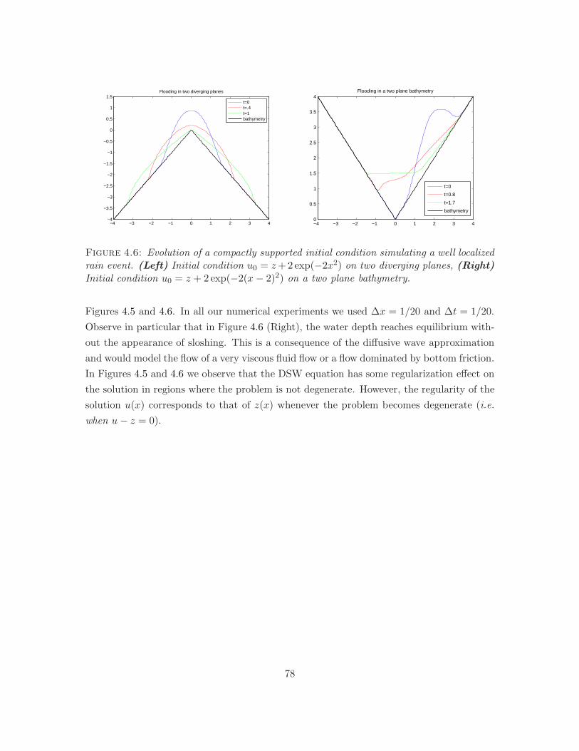
−4 −3 −2 −1 0 1 2 3 4−4

−3.5

−3

−2.5

−2

−1.5

−1

−0.5

0

0.5

1

1.5Flooding in two diverging planes

t=0t=.4t=1bathymetry

−4 −3 −2 −1 0 1 2 3 40

0.5

1

1.5

2

2.5

3

3.5

4Flooding in a two plane bathymetry

t=0

t=0.8

t=1.7

bathymetry

Figure 4.6: Evolution of a compactly supported initial condition simulating a well localizedrain event. (Left) Initial condition u0 = z+2exp(−2x2) on two diverging planes, (Right)Initial condition u0 = z + 2exp(−2(x− 2)2) on a two plane bathymetry.

Figures 4.5 and 4.6. In all our numerical experiments we used ∆x = 1/20 and ∆t = 1/20.

Observe in particular that in Figure 4.6 (Right), the water depth reaches equilibrium with-

out the appearance of sloshing. This is a consequence of the diffusive wave approximation

and would model the flow of a very viscous fluid flow or a flow dominated by bottom friction.

In Figures 4.5 and 4.6 we observe that the DSW equation has some regularization effect on

the solution in regions where the problem is not degenerate. However, the regularity of the

solution u(x) corresponds to that of z(x) whenever the problem becomes degenerate (i.e.

when u− z = 0).

78

Chapter 5

A Discontinuous Galerkin Method

In this Chapter we will study the approximation properties of numerical solutions to the

DSW equation, through the regularized initial/boundary-value problem (4.4), obtained us-

ing the LDG method. The overview of this Chapter is the following. For consistency we

present the well known notation in DG methods in section 5.1. Then we describe the details

of the LDG method in section 5.2. In section 5.2.2, we prove properties such as stability and

a priori error estimates for the numerical formulation of the LDG method. In section 5.3,

we show numerical simulations of the evolution of water depth profiles in 2D that capture

the salient features of: (i) an ideal dam break problem and (ii) water flow in a channel

containing vegetation.

5.1 Preliminaries

In this Chapter, we will consider a general triangulation τh of Ω ⊂ Rd into elements Ωe

of maximum diameter h > 0. We will denote with εi the set of all interior element faces,

with εD the set of all element faces along the Dirichlet boundary ΓD, and εN the set of all

element faces along the Newmann boundary ΓN . Now, note that if ε is an interior face in

the finite element mesh, then ε has two elements adjacent to it, we will denote them by Ω−e

and Ω+e . Also, if v and w are smooth real valued and vector valued functions, respectively,

defined on these elements, we will denote their traces on ε, from the interior of the element

Ω−e , as v− and w−; and from the exterior of the element Ω+

e , as v+ and w+. We will denote

by n− the outward normal vector to the element Ω−e at ε and by n+ the outward normal

vector to the element Ω+e at ε. The previous definition implies naturally that n+ = −n−.

79

We will define the average · and the jump J·K on the face ε as:

v =(v− + v+)

2, w =

(w− + w+)

2, (5.1)

JvK = v−n− + v+n+, JwK = w− · n− + w+ · n+ (5.2)

In this Chapter, we will also denote by (·, ·)E , the usual L2 inner product over an d-

dimensional domain E (as defined in section 2.3), and by 〈·, ·〉∂E , the (d − 1)-dimensional

integral over the surface ∂E. To simplify notation, we will omit the dependence on the

domain and denote with (·, ·) the integrals over the whole domain E = Ω, (·, ·)Ω.

5.2 The Local Discontinuous Galerkin Method

In order to motivate the LDG method it is appropriate to rewrite the nonlinear degenerate

parabolic IBVP (2.1) as a degenerate first order system of equations where u, ∇u, and

a(u,∇u), are now considered as independent unknowns:

ut −∇ · q = f on Ω × (0, T ]

q = ∇u on Ω × (0, T ]

q = a(u, q)q on Ω × (0, T ]

(5.3)

where

a(u, q) =(u− z)α

|q|1−γ, (5.4)

with initial and boundary conditions given as before by

u = u0 on Ω × 0q · n = BN on ∂Ω ∩ ΓN × (0, T ]

u = BD on ∂Ω ∩ ΓD × (0, T ]

(5.5)

where ∂Ω = Γ = ΓN + ΓD. Moreover, assuming u, q and q are smooth enough, we

multiply each equation in problem (5.3) by a local test functions w ∈Wh,e, v ∈ (Vh,e)d and

v ∈ (Vh,e)d respectively (where d = 1, 2, is the spatial dimension), and integrate by parts

over an element Ωe to obtain the local weak form of (5.3):

(ut, w)Ωe + (q,∇w)Ωe − 〈q · ne, w〉∂Ωe = (f,w)Ωe ∀w ∈Wh,e

(q, v)Ωe + (u,∇ · v)Ωe − 〈u,v · ne〉∂Ωe = 0 ∀ v ∈ (Vh,e)d

(q,v)Ωe − (a(u, q)q,v)Ωe = 0 ∀ v ∈ (Vh,e)d

(5.6)

80

where ne represents the outward normal vector in the faces of the element Ωe. The dis-

continuous Galerkin method consists of finding an approximation (U,Q, Q) to the solution

(u,q, q) of (5.6), of the form

U(x, t) =M∑

i=1

ζi(t)wi(x), Q(x, t) =N∑

i=1

µi(t)vi(x), and Q(x, t) =N∑

i=1

µi(t)vi(x). (5.7)

satisfying for all t ∈ [0, T ]

(Ut, w)Ωe + (Q,∇w)Ωe − 〈Q · ne, w〉∂Ωe = (f,w)Ωe ∀ w ∈Wh,e

(Q, v)Ωe + (U,∇ · v)Ωe − 〈U ,v · ne〉∂Ωe = 0 ∀ v ∈ (Vh,e)d

(Q,v)Ωe − (a(U, Q)Q,v)Ωe = 0 ∀ v ∈ (Vh,e)d

(5.8)

for every element Ωe in the domain Ω. In (5.7), w1, ..., wM are linearly independent piece-

wise polynomial functions in Wh = ∪Ωe∈Ω Wh,e and v1, ...,vN are vector valued linearly

independent piecewise polynomial functions in (Vh)d = ∪Ωe∈Ω (Vh,e)d. Generally speak-

ing, Wh,e and Vh,e are subspaces of H1(Ωe), and in practice they are chosen to be the set of

all polynomials of degree at most k inside every element Ωe. By construction, the approxi-

mants (U,Q, Q) may be discontinuous across element boundaries since no continuity across

elements is assumed in the basis functions spaces (Wh,e) and (Vh,e)d. As a consequence,

at a given face ε the functions (U,Q, Q) may be multi-valued. This is why the numerical

fluxes: Q and U are introduced in (5.8). Furthermore, in order to produce a meaningful

DG method and globally determine the coefficients ζi(t), µi(t), and µi(t) appearing in (5.7)

the numerical fluxes Q and U need to be carefully defined. This issue is clearly explained in

the context of elliptic problems in [22] and in [5], and in the context of nonlinear diffusion

problems in [19].

For the LDG method that we will analyse and implement, the numerical fluxes are chosen

in the following way:

U =

U if ε ∈ εi,

BD if ε ∈ ΓD,

U if ε ∈ ΓN ,

(5.9)

and

Q =

Q − σJUK if ε ∈ εi,

Q − σ(Un −BDn) if ε ∈ ΓD,

BN if ε ∈ ΓN ,

(5.10)

81

Furthermore, the basis functions spaces Wh,e and Vh,e will be chosen to be the same, thus

simplifying the coding as compared to standard mixed methods. Note that for the particular

choice of numerical fluxes introduced in (5.9) and (5.10), the numerical flux U does not

depend on Q. This makes it possible for the local variable Q to be solved in terms of U

by using the second equation of (5.8). This is a particular property that distinguishes the

LDG method from other DG schemes. The parameter σ appearing in the definition of the

numerical fluxes will be chosen carefully in order to enhance the stability and thus, the

accuracy of the method.

Remark 5.2.1. The fluxes defined in (5.9) and (5.10) are both consistent and conservative

as defined in [5] and [22].

The resulting LDG formulation is obtained in two steps. First, by summing over all

elements Ωe to find

(Ut, w) + (Q,∇w) − 〈Q, JwK〉εi− 〈Q · n, w〉∂Ω = (f,w) ∀ w ∈Wh

(Q, v) + (U,∇ · v) − 〈U , JvK〉εi− 〈U ,v · n〉∂Ω = 0 ∀ v ∈ (Wh)d

(a(U, Q)Q,v) − (Q,v) = 0 ∀ v ∈ (Wh)d

(5.11)

where we have denoted with (·, ·) =∑

e(·, ·)Ωe the sum of all element integrals. And second,

by substituting the values of the numerical fluxes (5.9) and (5.10) in (5.11)

(Ut, w) + (Q,∇w) − 〈Q, JwK〉εi+ 〈σJUK, JwK〉εi

+

−〈BN , w〉ΓN− 〈Q · n, w〉ΓD

+ 〈σ(U −BD), w〉ΓD= (f,w) ∀ w ∈Wh

(Q, v) + (U,∇ · v) − 〈U, JvK〉εi− 〈U, v · n〉ΓN

= 〈BD, v · n〉ΓD∀ v ∈ (Wh)d

(a(U, Q)Q,v) − (Q,v) = 0 ∀ v ∈ (Wh)d

(5.12)

where, for simplicity, we have denoted with

〈·, ·〉εi:=∑

e

〈·, ·〉∂Ωe\ Γ, 〈·, ·〉ΓN=∑

e

〈·, ·〉∂Ωe∩ ΓN, and 〈·, ·〉ΓD

=∑

e

〈·, ·〉∂Ωe∩ ΓD

the sum of the boundary integrals in all interior element boundaries εi, in all element bound-

aries along the Newman boundary ΓN , and in all element boundaries along the Dirichlet

boundary ΓD, respectively. In order to enforce the initial condition one must demand that

(U0, w) = (u0, w) ∀ w ∈Wh, t = 0. (5.13)

Note that using integration by parts for some of the terms in the second equation of (5.12),

82

the following expression holds,

(U,∇ · v) − 〈U, JvK〉εi− 〈U, v · n〉ΓN

= −(∇U,v) + 〈JUK, v〉εi+ 〈U, v · n〉ΓD

(5.14)

Based on the previous observation we will rewrite the LDG formulation for the IBVP (4.4)

as,

(Ut, w) + (Q,∇w) − 〈Q, JwK〉εi+ 〈σJUK, JwK〉εi

+

−〈BN , w〉ΓN− 〈Q · n, w〉ΓD

+ 〈σ(U −BD), w〉ΓD= (f,w) ∀ w ∈Wh

(Q, v) − (∇U, v) + 〈JUK, v〉εi+ 〈U, v · n〉ΓD

= 〈BD, v · n〉ΓD∀ v ∈ (Wh)d

(a(U, Q)Q,v) − (Q,v) = 0 ∀ v ∈ (Wh)d

(5.15)

Remark 5.2.2. It is clear that any continuous classical solution of problem (5.3)-(5.5) will

satisfy problem (5.15) since all terms involving jumps across elements J·K, will be zero and

all boundary terms will satisfy strongly the boundary conditions.

Remark 5.2.3. As in the numerical method presented in Chapter 4, the diffusion coefficient

a(u, q) in (5.4) will be approximated by the family of Lipschitz nondegenerate diffusion

coefficients of the form

aǫ(u, q) =βǫ(u)

|q|1−γ, (5.16)

and we will denote with β(·) any member of the family βǫ(·) in the subsequent analysis to

simplify the notation. Furthermore, note that any solution of the IBVP (4.4), as introduced

in Chapter 4, will also be a solution (5.3)-(5.5) with the regularized diffusion coefficient

(5.16).

Remark 5.2.4. The system of nonlinear ordinary differential equations arising from sub-

stituting the expressions of (U,Q, Q) given by (5.7) in (5.15) will be assumed to have at

least one solution. This assumption is based on the proof of existence of solutions of the

related problem (4.12) provided in Theorem 4.3.1.

5.2.1 Stability analysis

Even though the proof of Theorem 5.2.1 can be established as a Corollary of Theorem 5.2.2,

we present it here for clarity. Indeed, many of the mathematical manipulations presented

in the proof of Theorem 5.2.1 can be easily followed and will be used in the more elaborate

setting of the proof of Theorem 5.2.2.

83

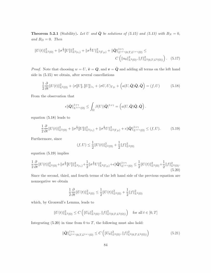
Theorem 5.2.1 (Stability). Let U and Q be solutions of (5.15) and (5.13) with BN = 0,

and BD = 0. Then

‖U(t)‖2L2(Ω) + ‖σ 1

2 JUK‖2L2(εi)

+ ‖σ 12U‖2

L2(ΓD) + ‖Q‖1+γL1+γ(0,T,L1+γ(Ω)

≤

C(‖u0‖2

L2(Ω), ‖f‖2L2(0,T ;L2(Ω))

). (5.17)

Proof. Note that choosing w = U , v = Q, and v = Q and adding all terms on the left hand

side in (5.15) we obtain, after several cancellations

1

2

∂

∂t‖U(t)‖2

L2(Ω) + 〈σJUK, JUK〉εi+ 〈σU,U〉ΓD

+(a(U, Q)Q, Q

)= (f, U) (5.18)

From the observation that

ǫ‖Q‖1+γL1+γ(Ω)

≤∫

Ωβ(U)|Q|1+γ =

(a(U, Q)Q, Q

).

equation (5.18) leads to

1

2

∂

∂t‖U(t)‖2

L2(Ω) + ‖σ 12 JUK‖2

L2(εi)+ ‖σ 1

2U‖2L2(ΓD) + ǫ‖Q‖1+γ

L1+γ(Ω)≤ (f, U). (5.19)

Furthermore, since

(f, U) ≤ 1

2‖U(t)‖2

L2(Ω) +1

2‖f‖2

L2(Ω)

equation (5.19) implies

1

2

∂

∂t‖U(t)‖2

L2(Ω)+‖σ 12 JUK‖2

L2(εi)+

1

2‖σ 1

2U‖2L2(ΓD)+ǫ‖Q‖1+γ

L1+γ(Ω)≤ 1

2‖U(t)‖2

L2(Ω)+1

2‖f‖2

L2(Ω).

(5.20)

Since the second, third, and fourth terms of the left hand side of the previous equation are

nonnegative we obtain

1

2

∂

∂t‖U(t)‖2

L2(Ω) ≤1

2‖U(t)‖2

L2(Ω) +1

2‖f‖2

L2(Ω)

which, by Gronwall’s Lemma, leads to

‖U(t)‖2L2(Ω) ≤ C

(‖U0‖2

L2(Ω), ‖f‖2L2(0,T ;L2(Ω))

)for all t ∈ [0, T ]

Integrating (5.20) in time from 0 to T , the following must also hold:

‖Q‖1+γL1+γ(0,T,L1+γ(Ω)

≤ C(‖U0‖2

L2(Ω), ‖f‖2L2(0,T ;L2(Ω))

)(5.21)

84

Likewise for the second and third terms of (5.20). Finally, by choosing w = U0 in the first

equation of (5.13) we obtain

(U0, U0) = (u0, U0) ≤1

2‖U0‖2

L2(Ω) +1

2‖u0‖2

L2(Ω)

which implies

‖U0‖2L2(Ω) ≤ ‖u0‖2

L2(Ω)

Thus, the result of the Theorem follows at once.

5.2.2 Continuous in time a priori error analysis

In this section we will study how close (possibly nonunique) solutions to the LDG approxi-

mation problem (5.15), U , are to the true weak solution u of problem (5.3)-(5.5) with the

regularized diffusion coefficient (5.16). We will focus the present analysis to the case when

∇u ∈ L∞(0, T, L∞(Ω)). In the following paragraphs we will assume that u is regular enough

so that:

(i) the continuous interpolant of u in Pk, u, is well defined and satisfies

∫

Ω(u− u)w = 0 ∀ w ∈ Pk (5.22)

(ii) the L2-projection of q in (Pk)d, q, is well defined and given by

∫

Ω(q − q)v = 0 ∀ v ∈ (Pk)d (5.23)

(iii) inside every element Ωe,

ˆq = ∇u. (5.24)

Further assumptions include that βǫ(u), βǫ(U),∇u,∇U ∈ L∞(0, T, L∞(Ω)).

Theorem 5.2.2. Let (u, q,q) ∈ L∞(Ω)× (L∞(Ω))d × (L∞(Ω))d be the solution of problem

(5.3)-(5.5) and let U, Q,Q be a solution of problem (5.15). Let χu = u − u, χq = q − ˆq

85

and χq = q − q. Further, assume that ∇u, Q ∈ L∞(0, T, L∞(Ω)). Then for all t ∈ [0, T ]

‖U(t) − u(t)‖2L2(Ω) + ‖Q − q‖2

L2(0,T,L2(Ω))+

+

∫ T

0

(‖σ 1

2 JU(t) − u(t)K‖2L2(εi)

+ ‖σ 12 (U(t) − u(t)) ‖2

L2(ΓD)

)≤

‖χu(t)‖2L2(Ω) + ‖σ 1

2χu‖2L2(ΓD) + ‖χq‖2

L2(Ω) + C(‖ξu(0)‖2

L2(Ω) + ‖χu‖2L2(0,T,L2(Ω))+

+

∫ T

0

(‖σ− 1

2χq‖2L2(εi)

+ ‖σ 12χu‖2

L2(ΓD)

)+

∫ T

0

∫

Ω|χq|2γ

). (5.25)

Proof. Since any solution u of (5.3)-(5.5) satisfies the weak form (5.15), the following three

equations must hold:

(Ut − ut, w) + (Q − q,∇w) − 〈Q − q, JwK〉εi+ 〈σJU − uK, JwK〉εi

+

− 〈(Q − q) · n, w〉ΓD+ 〈σ(U − u), w〉ΓD

= (ut − ut, w) + (q − q,∇w) − 〈q − q, JwK〉εi+ 〈σJu− uK, JwK〉εi

+

− 〈(q − q) · n, w〉ΓD+ 〈σ(u− u), w〉ΓD

, (5.26)

(Q − ˆq, v) − (∇(U − u), v) + 〈JU − uK, v〉εi+ 〈U − u, v · n〉ΓD

= (q − ˆq, v) − (∇(u− u), v) + 〈Ju− uK, v〉εi+ 〈u− u, v · n〉ΓD

, (5.27)

and

(

β(U)

(Q

|Q|1−γ−

ˆq

|ˆq|1−γ

)

,v

)

− (Q − q,v) =

(

β(u)

(q

|q|1−γ−

ˆq

|ˆq|1−γ

)

,v

)

+

− (q − q,v) −(

(β(U) − β(u))ˆq

|ˆq|1−γ,v

)

. (5.28)

Note that the second term of the right hand side of (5.26) and the second term of the right

hand side of (5.28) are zero since q satisfies (5.23). Thus,

(q − q,∇w) = 0 and (q − q,v) = 0

To simplify notation, let ξu = U − u, ξq = Q − ˆq and ξq = Q − q. Now, choosing w = ξu,

v = ξq, and v = ξq, and adding equations (5.26),(5.27), and (5.28) we obtain, after multiple

cancellations:

86

1

2

∂

∂t‖ξu(t)‖2

L2(Ω) + 〈σJξuK, JξuK〉εi+ 〈σξu, ξu〉ΓD

+

(β(U)

(Q

|Q|1−γ−

ˆq

|ˆq|1−γ

), ξq

)=

((χu)t, ξu) − 〈χq, JξuK〉εi+ 〈σJχuK, JξuK〉εi

+

+ (χq, ξq) − (∇χu, ξq) + 〈JχuK, ξq〉εi+ 〈σχu, ξu〉ΓD

+

(β(u)

(q

|q|1−γ−

ˆq

|ˆq|1−γ

), ξq

)−(

(β(U) − β(u))ˆq

|ˆq|1−γ, ξq

)(5.29)

Furthermore, from the result of Lemma 4.2.2 and provided β(U) ≥ ǫ > 0 the following must

hold

γǫA‖ξq‖2L2(Ω) ≤

(β(U)

(Q

|Q|1−γ−

ˆq

|ˆq|1−γ

), Q − ˆq

)(5.30)

where A := inf(0,T )×Ω

(A0) = inf(0,T )×Ω

1/(‖Q‖L∞(0,T,L∞(Ω)) + ‖ˆq‖L∞(0,T,L∞(Ω)))

)1−γ

Using the triangle inequality in (5.29) and using the previous inequality, we can establish

that

1

2

∂

∂t‖ξu(t)‖2

L2(Ω) + ‖σ 12 JξuK‖2

L2(εi)+ ‖σ 1

2 ξu‖2L2(ΓD) + γǫA‖ξq‖2

L2(Ω) ≤10∑

i=1

Ti (5.31)

where Ti, i = 1, ..., 9, are the terms arising from the right hand side of (5.29). We now

proceed to bound the terms |Ti| for i = 1, ..., 9.

Note that T1 is zero by (5.22). For T2, we multiply and divide by σ12 to get

T2 = 〈σ− 12 χq, σ

12 JξuK〉εi

≤ ǫ12‖σ 1

2 JξuK‖2L2(εi)

+1

2ǫ1‖σ− 1

2 χq‖2L2(εi)

(5.32)

For T3

T3 = 〈σ 12 JχuK, σ

12 JξuK〉εi

≤ 1

2‖σ 1

2 JξuK‖2L2(εi)

+1

2‖σ 1

2 JχuK‖2L2(εi)

(5.33)

Note that the choice of ˆq and u in (5.24) and (5.22), respectively, and the fact that ξq ∈ Pk

ensures the three following equalities:

‖σ 12 JχuK‖2

L2(εi)= 0, T6 = 〈JχuK, ξq〉εi

= 0, (5.34)

and

T4 = (χq, ξq) = (∇χu, ξq) = T5. (5.35)

Thus, T4 − T5 = 0 and T6 = 0.

87

For term T7 we have the following inequality

T7 = 〈σχu, ξu〉ΓD≤ 1

2‖σ 1

2χu‖2L2(ΓD) +

1

2‖σ 1

2 ξu‖2L2(ΓD) (5.36)

As for terms T8 and T9, note that

T8 =

∫

Ωβ(u)

(q

|q|1−γ−

ˆq

|ˆq|1−γ

)

ξq ≤ 2

γM

∫

Ω|χq|γ |ξq| (5.37)

≤ 2

γM

(1

2ǫ2

∫

Ω|χq|2γ +

ǫ22‖ξq‖2

L2(Ω)

)

and for T9 =

(

(β(U) − β(u))ˆq

|ˆq|1−γ, ξq

)

we have

T9 ≤ M∗

∫

Ω|u− U ||ˆq|γ |ξq| (5.38)

≤ M∗‖ˆq‖γL∞(Ω)‖u− U‖L2(Ω)‖ξq‖L2(Ω)

≤ M∗‖ˆq‖γL∞(Ω)

(1

2ǫ3(‖χu‖2

L2(Ω) + ‖ξu‖2L2(Ω)) +

ǫ32‖ξq‖2

L2(Ω)

),

where M = ‖β(u)‖L∞(Ω) and M∗ = α max(‖β(u)‖L∞(Ω), ‖β(U)‖L∞(Ω))α−1.

From (5.31) and (5.32), (5.33), (5.35), (5.34), (5.36), (5.37), and (5.38) and choosing ǫ1,

ǫ2 and ǫ3 small enough so that for ǫ and ǫ∗ small positive numbers, 0 < ǫ ≤ γǫ A −(1γMǫ2 + 1

2M∗‖ˆq‖γ

L∞ǫ3

)and 0 < ǫ∗ ≤ 1

2 (1 − ǫ1), we obtain

1

2

∂

∂t‖ξu(t)‖2

L2(Ω) + ǫ∗‖σ 12 JξuK‖2

L2(εi)+

1

2‖σ 1

2 ξu‖2L2(ΓD) + ǫ ‖ξq‖2

L2(Ω) ≤

C(‖ξu‖2

L2(Ω) + ‖χu‖2L2(Ω)+

+‖σ− 12 χq‖2

L2(εi)+ ‖σ 1

2χu‖2L2(ΓD) +

∫

Ω|χq|2γ

)(5.39)

Since the second, third, and fourth terms of the left hand side in the previous inequality

are nonnegative, we can use Gronwall’s Lemma to find that for all t ∈ [0, T ],

‖ξu(t)‖2L2(Ω) ≤ C

(‖ξu(0)‖2

L2(Ω) + ‖χu‖2L2(0,T,L2(Ω))+

+

∫ T

0

(‖σ− 1

2χq‖2L2(εi)

+ ‖σ 12χu‖2

L2(ΓD)

)+

∫ T

0

∫

Ω|χq|2γ

)(5.40)

88

Likewise, integrating (5.39) in time from 0 to T , we can establish the boundedness of the

three remaining terms of the left hand side of (5.39):

∫ T

0

(‖σ 1

2 JξuK‖2L2(εi)

+ ‖σ 12 ξu‖2

L2(ΓD)

)and ‖ξq‖2

L2(0,T,L2(Ω)). (5.41)

Finally, observe that

‖U(t) − u(t)‖2L2(Ω) ≤ ‖ξu(t)‖2

L2(Ω) + ‖χu(t)‖2L2(Ω),

‖Q − q‖2L2(Ω) ≤ ‖ξq‖2

L2(Ω) + ‖χq‖2L2(Ω),

‖σ 12 (U(t) − u(t)) ‖2

L2(ΓD) ≤ ‖σ 12 ξu‖2

L2(ΓD) + ‖σ 12χu‖2

L2(ΓD)

and

‖σ 12 JU(t) − u(t)K‖2

L2(εi)= ‖σ 1

2 JξuK‖2L2(εi)

, since ‖σ 12 Ju(t)K‖2

L2(εi)= 0.

The result of the Theorem follows immediately.

Corollary 5.2.1. If u ∈ W 1,∞(Ω) ∩ Hk+1(Ω), q,q ∈ L∞(Ω) are the solution of problem

(5.4) and U, Q,Q are a solution of problem (5.15), constructed with piecewise polynomials

of degree at most k. Then for all t ∈ [0, T ] and σ = 1h

‖U(t) − u(t)‖L2(Ω) + ‖Q(t) − q(t)‖L2(0,T,L2(Ω))+

+

∫ T

0

1

h

(‖JU(t) − u(t)K‖L2(εi) + ‖ (U(t) − u(t)) ‖L2(ΓD)

)≤ C(T )hkγ

(∫ T

0‖u(t)‖2γ

Hk+1(Ω)

) 12

(5.42)

Proof. Based on the result of Theorem 5.2.2, we need to show how all the terms of the right

hand side of (5.25) are bounded. For such regularity on u, the approximation estimates

shown in Lemma 2.4.1 must hold. Thus,

‖χu(t)‖2L2(Ω) ≤ C h2(k+1) ‖u‖2

Hk+1(Ω), (5.43)

‖χq‖2[L2(Ω)]2 ≤ C h2k ‖u‖2

[Hk+1]2 (Ω), (5.44)

‖(χu)t‖2L2(0,T,L2(Ω)) ≤ C(T ) h2(k+1)

∫ T

0‖u‖2

Hk+1(Ω), (5.45)

Using the approximation estimates from Lemma 2.5.1 the following must also hold:

‖σ 12χu‖2

L2(ΓD) ≤ ‖σ 12χu‖2

L2(∂Ω) ≤1

hC h2k+1‖u‖2

Hk+1(Ω) ≤ C h2k‖u‖2Hk+1(Ω) (5.46)

89

Note also that

∫ T

0

∫

Ω|χq|2γ ≤

∫ T

0

(∫

Ω|χq|2

) 2γ2

|Ω|1−γ =

∫ T

0‖χq‖2γ

L2(Ω)|Ω|1−γ

≤ C(T )h2kγ ‖u‖2γHk+1(Ω)

(5.47)

and using Lemma 2.5.1 for the union of elements,

∫ T

0‖σ− 1

2 χq‖2L2(εi)

≤∫ T

0h

∥∥∥∥

β(u)

q

|q|1−γ− q

∥∥∥∥2

L2(εi)

≤∫ T

0h h2k+1

∥∥∥∥β(u)q

|q|1−γ

∥∥∥∥2

Hk+1(Ω)

≤∫ T

0h2(k+1)‖β(u)‖2

L∞(Ω) ‖|q|γ‖2Hk+1(Ω) (5.48)

From the result of Theorem 5.2.2, and noting that the leading term of estimates (5.43)-(5.48)

for small h is the one given by (5.47), the following must hold

‖U(t) − u(t)‖2L2(Ω) + ‖Q(t) − q(t)‖2

L2(0,T,L2(Ω))+

+

∫ T

0

1

h

(‖JU(t) − u(t)K‖2

L2(εi)+ ‖ (U(t) − u(t)) ‖2

L2(ΓD)

)≤ C(T )h2kγ

∫ T

0‖u(t)‖2γ

Hk+1(Ω)

(5.49)

The result of the Theorem follows from the observation that for nonnegative numbers

p, q, r, s, f , the fact that p2 + q2 + r2 + s2 ≤ f2 implies that there exists a positive con-

stant C such that p+ q + r + s ≤ C f . This concludes the proof.

5.3 Numerical Experiments. 2D

In this section, we present the results of some numerical experiments aimed at solving two

ideal 2D problems: a dam break event, and flow in a channel with vegetation resulting from

a dam break event. The main motivation to show these results is to provide the reader with

convincing evidence that the DSW equation captures the physics of the aforementioned

ideal problems. In fact, the setting of the simulated flow in a channel with vegetation was

inspired by an actual experiment shown in [13]. In future work we intend to simulate the

results of this real life experiment in order to verify that the computational results match

the measurements presented in [13].

90

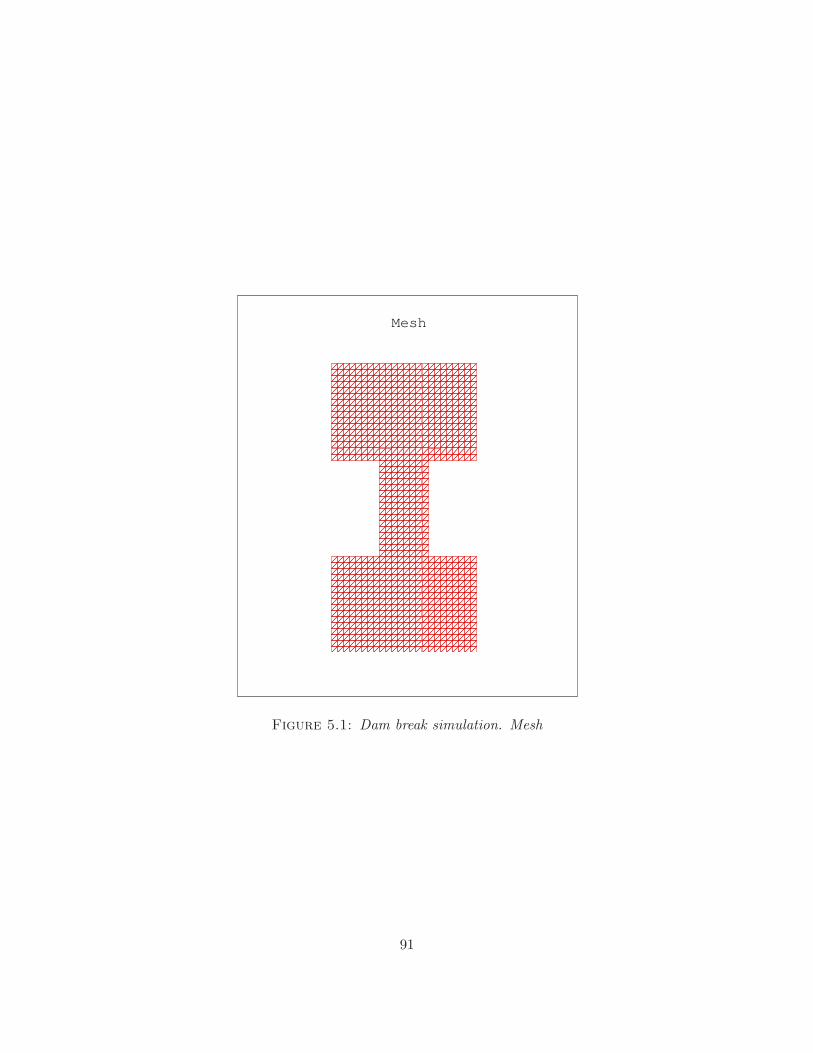
Mesh

Figure 5.1: Dam break simulation. Mesh

91

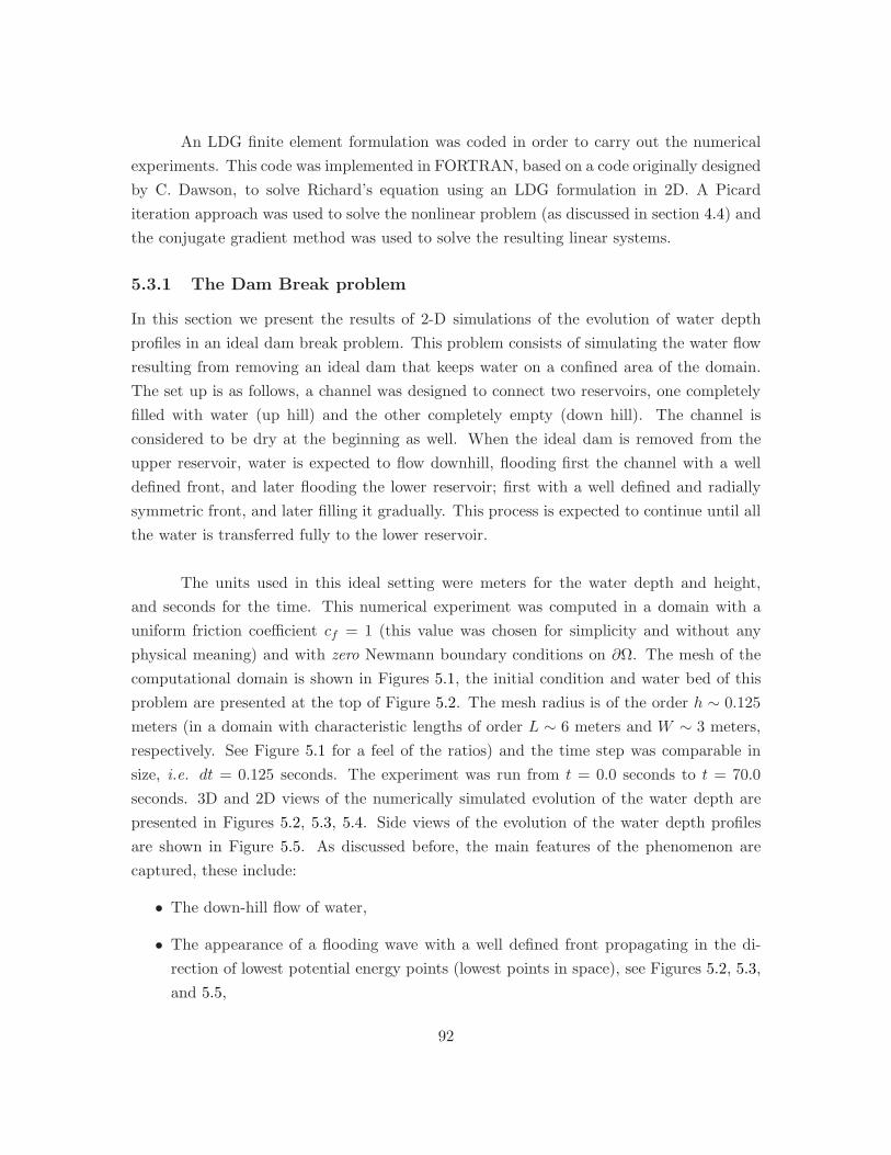
An LDG finite element formulation was coded in order to carry out the numerical

experiments. This code was implemented in FORTRAN, based on a code originally designed

by C. Dawson, to solve Richard’s equation using an LDG formulation in 2D. A Picard

iteration approach was used to solve the nonlinear problem (as discussed in section 4.4) and

the conjugate gradient method was used to solve the resulting linear systems.

5.3.1 The Dam Break problem

In this section we present the results of 2-D simulations of the evolution of water depth

profiles in an ideal dam break problem. This problem consists of simulating the water flow

resulting from removing an ideal dam that keeps water on a confined area of the domain.

The set up is as follows, a channel was designed to connect two reservoirs, one completely

filled with water (up hill) and the other completely empty (down hill). The channel is

considered to be dry at the beginning as well. When the ideal dam is removed from the

upper reservoir, water is expected to flow downhill, flooding first the channel with a well

defined front, and later flooding the lower reservoir; first with a well defined and radially

symmetric front, and later filling it gradually. This process is expected to continue until all

the water is transferred fully to the lower reservoir.

The units used in this ideal setting were meters for the water depth and height,

and seconds for the time. This numerical experiment was computed in a domain with a

uniform friction coefficient cf = 1 (this value was chosen for simplicity and without any

physical meaning) and with zero Newmann boundary conditions on ∂Ω. The mesh of the

computational domain is shown in Figures 5.1, the initial condition and water bed of this

problem are presented at the top of Figure 5.2. The mesh radius is of the order h ∼ 0.125

meters (in a domain with characteristic lengths of order L ∼ 6 meters and W ∼ 3 meters,

respectively. See Figure 5.1 for a feel of the ratios) and the time step was comparable in

size, i.e. dt = 0.125 seconds. The experiment was run from t = 0.0 seconds to t = 70.0

seconds. 3D and 2D views of the numerically simulated evolution of the water depth are

presented in Figures 5.2, 5.3, 5.4. Side views of the evolution of the water depth profiles

are shown in Figure 5.5. As discussed before, the main features of the phenomenon are

captured, these include:

• The down-hill flow of water,

• The appearance of a flooding wave with a well defined front propagating in the di-

rection of lowest potential energy points (lowest points in space), see Figures 5.2, 5.3,

and 5.5,

92

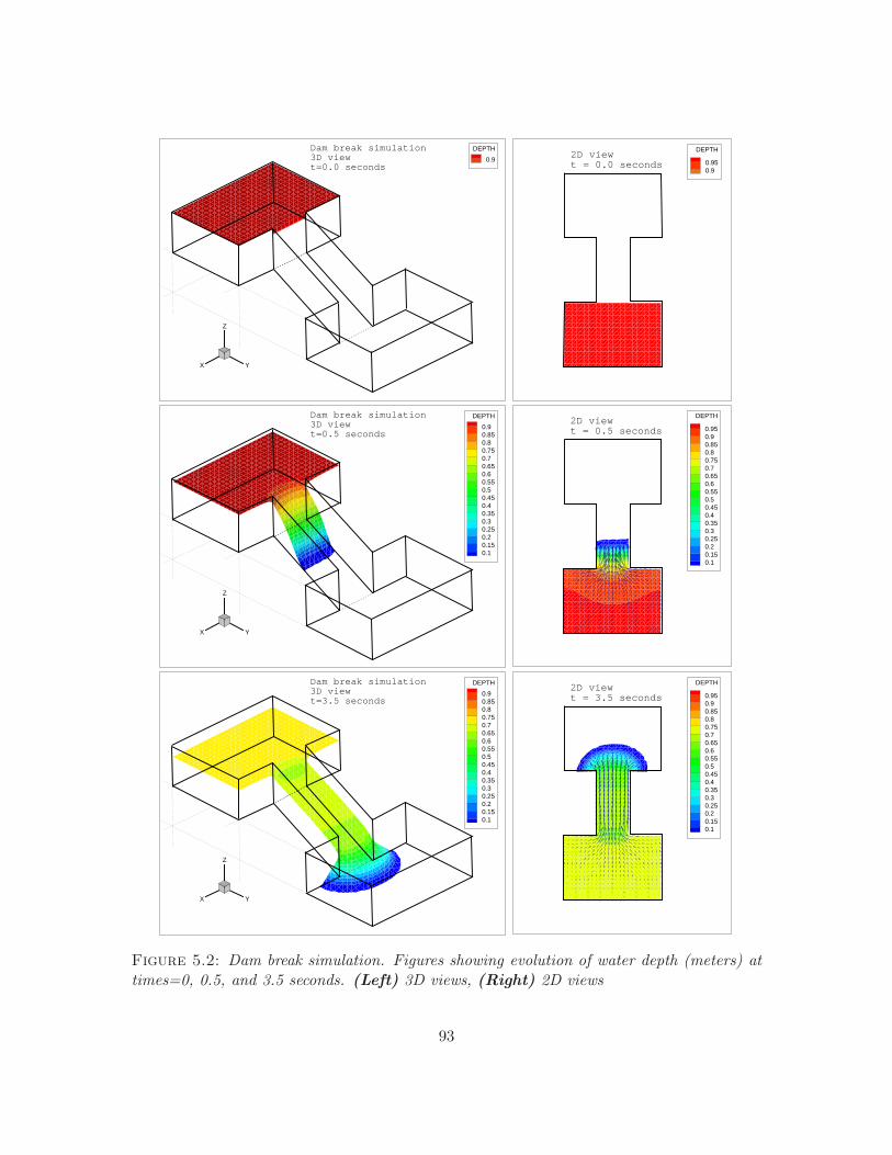
X Y

Z

DEPTH

0.9

Dam break simulation3D viewt=0.0 seconds

DEPTH

0.950.9

2D viewt = 0.0 seconds

X Y

Z

DEPTH

0.90.850.80.750.70.650.60.550.50.450.40.350.30.250.20.150.1

Dam break simulation3D viewt=0.5 seconds

DEPTH

0.950.90.850.80.750.70.650.60.550.50.450.40.350.30.250.20.150.1

2D viewt = 0.5 seconds

X Y

Z

DEPTH

0.90.850.80.750.70.650.60.550.50.450.40.350.30.250.20.150.1

Dam break simulation3D viewt=3.5 seconds

DEPTH

0.950.90.850.80.750.70.650.60.550.50.450.40.350.30.250.20.150.1

2D viewt = 3.5 seconds

Figure 5.2: Dam break simulation. Figures showing evolution of water depth (meters) attimes=0, 0.5, and 3.5 seconds. (Left) 3D views, (Right) 2D views

93

X Y

Z

DEPTH

0.90.850.80.750.70.650.60.550.50.450.40.350.30.250.20.150.1

Dam break simulation3D viewt=5.0 seconds

DEPTH

0.950.90.850.80.750.70.650.60.550.50.450.40.350.30.250.20.150.1

2D viewt = 5.0 seconds

X Y

Z

DEPTH

0.90.850.80.750.70.650.60.550.50.450.40.350.30.250.20.150.1

Dam break simulation3D viewt=7.0 seconds

DEPTH

0.950.90.850.80.750.70.650.60.550.50.450.40.350.30.250.20.150.1

2D viewt = 7.0 seconds

X Y

Z

DEPTH

0.90.850.80.750.70.650.60.550.50.450.40.350.30.250.20.150.1

Dam break simulation3D viewt=9.0 seconds

DEPTH

0.950.90.850.80.750.70.650.60.550.50.450.40.350.30.250.20.150.1

2D viewt = 9.0 seconds

Figure 5.3: Dam break simulation. Figures showing evolution of water depth (meters) attimes=5.0, 7.0, and 9.0 seconds. (Left) 3D views, (Right) 2D views

94

X Y

Z

DEPTH

0.90.850.80.750.70.650.60.550.50.450.40.350.30.250.20.150.1

Dam break simulation3D viewt=34.0 seconds

DEPTH

0.950.90.850.80.750.70.650.60.550.50.450.40.350.30.250.20.150.1

2D viewt = 34.0 seconds

X Y

Z

DEPTH

0.90.850.80.750.70.650.60.550.50.450.40.350.30.250.20.150.1

Dam break simulation3D viewt=54.0 seconds

DEPTH

0.950.90.850.80.750.70.650.60.550.50.450.40.350.30.250.20.150.1

2D viewt = 54.0 seconds

X Y

Z

DEPTH

0.90.850.80.750.70.650.60.550.50.450.40.350.30.250.2

Dam break simulation3D viewt=70.0 seconds

DEPTH

0.950.90.850.80.750.70.650.60.550.50.450.40.350.30.250.2

2D viewt = 70.0 seconds

Figure 5.4: Dam break simulation. Figures showing evolution of water depth (meters) attimes=34.0, 54.0, and 70.0 seconds. (Left) 3D views, (Right) 2D views

95

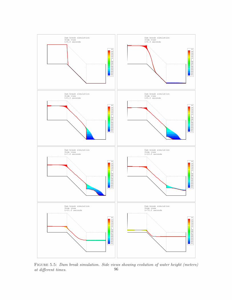
H

1.51.41.31.21.110.90.80.70.60.50.40.30.20.1

Dam break simulationSide viewt=0.0 seconds

H

1.51.41.31.21.110.90.80.70.60.50.40.30.20.1

Dam break simulationSide viewt=0.5 seconds

H

1.51.41.31.21.110.90.80.70.60.50.40.30.20.1

Dam break simulationSide viewt=3.5 seconds

H

1.51.41.31.21.110.90.80.70.60.50.40.30.20.1

Dam break simulationSide viewt=5.5 seconds

H

1.51.41.31.21.110.90.80.70.60.50.40.30.20.1

Dam break simulationSide viewt=7.0 seconds

H

1.51.41.31.21.110.90.80.70.60.50.40.30.20.1

Dam break simulationSide viewt=10.0 seconds

H

1.51.41.31.21.110.90.80.70.60.50.40.30.20.1

Dam break simulationSide viewt=21.0 seconds

H

1.51.41.31.21.110.90.80.70.60.50.40.30.20.1

Dam break simulationSide viewt=70.0 seconds

Figure 5.5: Dam break simulation. Side views showing evolution of water height (meters)at different times. 96

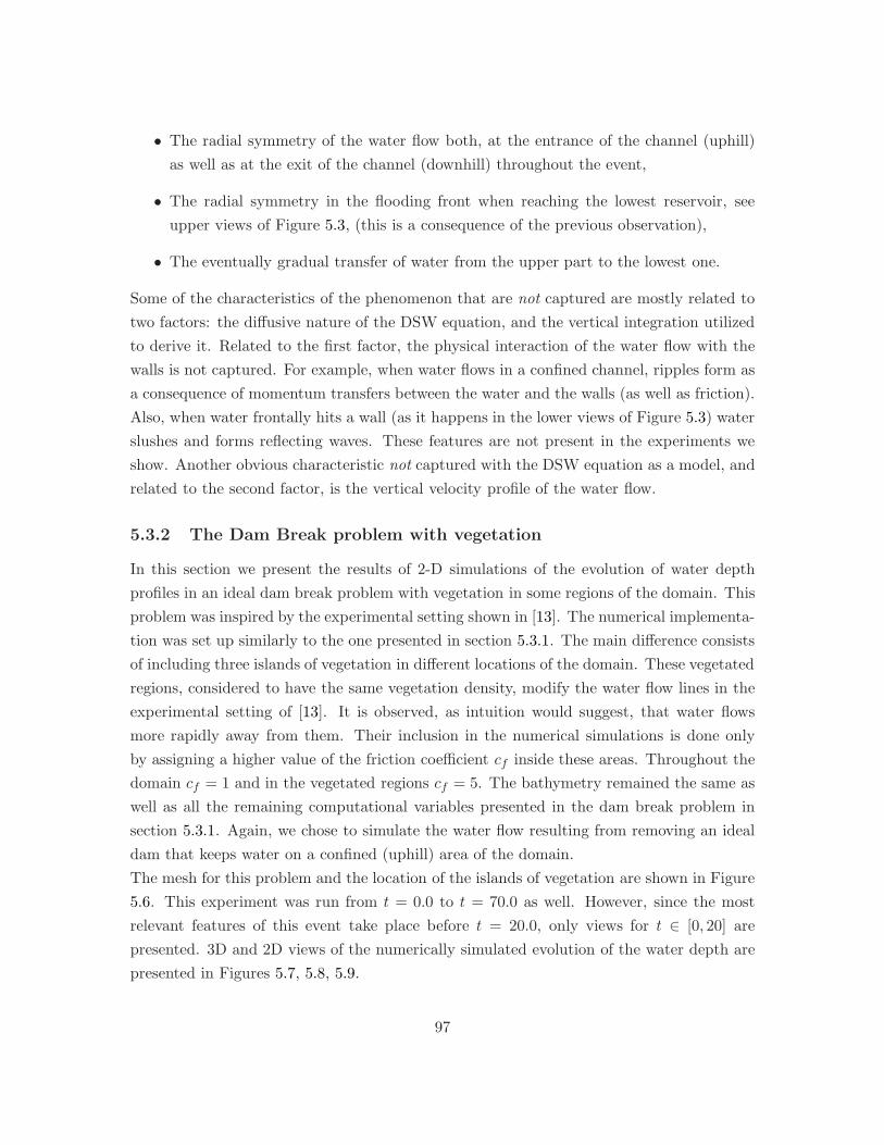
• The radial symmetry of the water flow both, at the entrance of the channel (uphill)

as well as at the exit of the channel (downhill) throughout the event,

• The radial symmetry in the flooding front when reaching the lowest reservoir, see

upper views of Figure 5.3, (this is a consequence of the previous observation),

• The eventually gradual transfer of water from the upper part to the lowest one.

Some of the characteristics of the phenomenon that are not captured are mostly related to

two factors: the diffusive nature of the DSW equation, and the vertical integration utilized

to derive it. Related to the first factor, the physical interaction of the water flow with the

walls is not captured. For example, when water flows in a confined channel, ripples form as

a consequence of momentum transfers between the water and the walls (as well as friction).

Also, when water frontally hits a wall (as it happens in the lower views of Figure 5.3) water

slushes and forms reflecting waves. These features are not present in the experiments we

show. Another obvious characteristic not captured with the DSW equation as a model, and

related to the second factor, is the vertical velocity profile of the water flow.

5.3.2 The Dam Break problem with vegetation

In this section we present the results of 2-D simulations of the evolution of water depth

profiles in an ideal dam break problem with vegetation in some regions of the domain. This

problem was inspired by the experimental setting shown in [13]. The numerical implementa-

tion was set up similarly to the one presented in section 5.3.1. The main difference consists

of including three islands of vegetation in different locations of the domain. These vegetated

regions, considered to have the same vegetation density, modify the water flow lines in the

experimental setting of [13]. It is observed, as intuition would suggest, that water flows

more rapidly away from them. Their inclusion in the numerical simulations is done only

by assigning a higher value of the friction coefficient cf inside these areas. Throughout the

domain cf = 1 and in the vegetated regions cf = 5. The bathymetry remained the same as

well as all the remaining computational variables presented in the dam break problem in

section 5.3.1. Again, we chose to simulate the water flow resulting from removing an ideal

dam that keeps water on a confined (uphill) area of the domain.

The mesh for this problem and the location of the islands of vegetation are shown in Figure

5.6. This experiment was run from t = 0.0 to t = 70.0 as well. However, since the most

relevant features of this event take place before t = 20.0, only views for t ∈ [0, 20] are

presented. 3D and 2D views of the numerically simulated evolution of the water depth are

presented in Figures 5.7, 5.8, 5.9.

97

Mesh

"Vegetated areas"

Figure 5.6: Dam break simulation with vegetation. Mesh

98

X Y

Z

DEPTH

0.950.9

Dam break simulation3D viewt=0.0 seconds

DEPTH

0.950.9

2D viewt = 0.0 seconds

X Y

Z

DEPTH

0.950.90.850.80.750.70.650.60.550.50.450.40.350.30.250.20.150.1

Dam break simulation3D viewt=1.0 seconds

DEPTH

0.950.90.850.80.750.70.650.60.550.50.450.40.350.30.250.20.150.1

2D viewt = 1.0 seconds

X Y

Z

DEPTH

0.950.90.850.80.750.70.650.60.550.50.450.40.350.30.250.20.150.1

Dam break simulation3D viewt=3.0 seconds

DEPTH

0.950.90.850.80.750.70.650.60.550.50.450.40.350.30.250.20.150.1

2D viewt = 3.0 seconds

Figure 5.7: Dam break simulation with vegetation. Figures showing evolution of waterdepth (meters) at times=0, 1.0, and 3.0 seconds. (Left) 3D views, (Right) 2D views

99

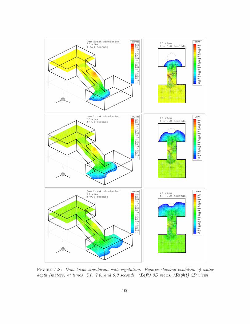
X Y

Z

DEPTH

0.950.90.850.80.750.70.650.60.550.50.450.40.350.30.250.20.150.1

Dam break simulation3D viewt=5.0 seconds

DEPTH

0.950.90.850.80.750.70.650.60.550.50.450.40.350.30.250.20.150.1

2D viewt = 5.0 seconds

X Y

Z

DEPTH

0.950.90.850.80.750.70.650.60.550.50.450.40.350.30.250.20.150.1

Dam break simulation3D viewt=7.0 seconds

DEPTH

0.950.90.850.80.750.70.650.60.550.50.450.40.350.30.250.20.150.1

2D viewt = 7.0 seconds

X Y

Z

DEPTH

0.950.90.850.80.750.70.650.60.550.50.450.40.350.30.250.20.150.1

Dam break simulation3D viewt=9.0 seconds

DEPTH

0.950.90.850.80.750.70.650.60.550.50.450.40.350.30.250.20.150.1

2D viewt = 9.0 seconds

Figure 5.8: Dam break simulation with vegetation. Figures showing evolution of waterdepth (meters) at times=5.0, 7.0, and 9.0 seconds. (Left) 3D views, (Right) 2D views

100

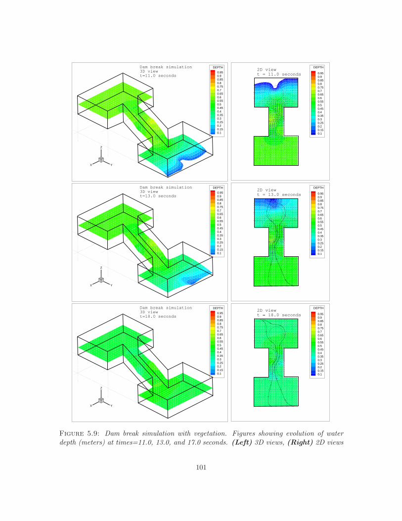
X Y

Z

DEPTH

0.950.90.850.80.750.70.650.60.550.50.450.40.350.30.250.20.150.1

Dam break simulation3D viewt=11.0 seconds

DEPTH

0.950.90.850.80.750.70.650.60.550.50.450.40.350.30.250.20.150.1

2D viewt = 11.0 seconds

X Y

Z

DEPTH

0.950.90.850.80.750.70.650.60.550.50.450.40.350.30.250.20.150.1

Dam break simulation3D viewt=13.0 seconds

DEPTH

0.950.90.850.80.750.70.650.60.550.50.450.40.350.30.250.20.150.1

2D viewt = 13.0 seconds

X Y

Z

DEPTH

0.950.90.850.80.750.70.650.60.550.50.450.40.350.30.250.20.150.1

Dam break simulation3D viewt=18.0 seconds

DEPTH

0.950.90.850.80.750.70.650.60.550.50.450.40.350.30.250.20.150.1

2D viewt = 18.0 seconds

Figure 5.9: Dam break simulation with vegetation. Figures showing evolution of waterdepth (meters) at times=11.0, 13.0, and 17.0 seconds. (Left) 3D views, (Right) 2D views

101

Figures 5.7-5.9 show very good agreement with the expected features of the phe-

nomenon. In particular, they clearly display the fact that, as expected, water flows more

rapidly away from the vegetated areas. Also, the flooding front propagates throughout the

domain in a way that qualitatively captures the expected dynamics. Again, the limitations

of the DSW equation as a model appear as described in the previous section.

102

Chapter 6

Concluding Remarks and Future

Work

In this dissertation, a mathematical model aimed at describing the dynamics of shallow

water flow in environments such as wetlands is studied in depth. A concise derivation of

this mathematical model is proposed in this work as a combination of, scaling arguments

that characterize the diffusive wave approximation of the shallow water equations (DSW),

and experimental studies aimed at understanding the dynamics of shallow water flow in

vegetated areas. The emerging initial boundary value problem (IBVP), associated to this

model, is stated in Chapter 2 as the IBVP (2.1).

The mathematical properties of the IBVP (2.1) are initially explored in Chapter 1,

in the context of the theory of doubly nonlinear parabolic equations, by carefully identifying

an alternative formulation of the IBVP (2.1) for flat topographies, namely the IBVP (1.7).

In Chapter 3, a study of basic properties of nonnegative solutions for the DSW equation

is presented in a hydrological context. Furthermore, an original proof of existence of weak

solutions using constructive techniques that directly lead to the implementation of numer-

ical algorithms to obtain approximate solutions is proposed. Also, alternative proofs of the

most relevant results existing in the literature are presented. The open problem that arises,

when topographic effects are considered (obstacle problem) in the DSW, is discussed and

introduced as a new avenue of research in the area of theoretical PDEs.

In Chapter 4 the results of a numerical approach to study the properties of solu-

tions of the IBVP (2.1) are shown. The emphasis is placed in analysing the mathematical

properties of the partial differential equation appearing in the IBVP (2.1), using a regu-

103

larization technique introduced in Chapter 3. The analysis is carried out in order to find

estimates for the error between numerical solutions, constructed using the Galerkin method,

and true solutions of this equation. A proof that the numerical solutions converge to the

true solution of the regularized DSW equation (4.4) under certain physically consistent con-

ditions is presented. These conditions emerge from physical consistency and are given by

u ∈ L∞(0, T ;L∞(Ω)) and ∇u ∈ L∞(0, T ;L∞(Ω)). The absence of appropriate conditions

leading to a proof to ensure uniqueness of solutions of the DSW equation, in its general

form (2.1), imposes restrictions in the analysis shown, and as a consequence the analytical

a priori error estimates presented in sections 4.3.3 and 4.3.4 are not optimal. In section 4.4,

numerical evidence that shows that the proposed numerical method converges to the true

weak solution of the IBVP (2.1) is presented even when the conditions for Theorem 4.3.2 to

hold are not met. In fact, it is found that in regions where the solution does not degenerate

(u − z > 0) the numerical method reaches optimal convergence rates. Despite the fact

that the IBVP (2.1) has not been fully studied analytically when z 6= 0, properties such as

boundedness and existence of compactly supported solutions, finite speed of propagation of

disturbances, and extinction in finite time found in the 1-D case when z = 0 in [35], [6], and

[2], were found to persist for a bounded and smooth bathymetry z 6= 0, based on numerical

evidence.

In Chapter 4, solutions of the DSW equation that locally violate some of the essen-

tial assumptions used to derive the DSW equation from the Navier-Stokes equations are

introduced. Such is the case for the family of compactly supported Barenblatt solutions

exhibited when z = 0 in section 4.4.1. The gradient of these solutions (water surface slope)

is not comparable to the gradient of the bathymetry ∇z close to the free boundary. A

more extreme case of solutions that violate the uniform flow conditions happen even when

the DSW equation becomes the PME (z = 0 and γ = 1) in two or higher dimensions.

In Chapter 19 of [62], Vazquez shows that there exists a class of solutions called focusing

solutions that exhibit no local regularity on the gradient in subsets of Ω. The existence of

these kinds of solutions serves as a reminder of the limitations of using the DSW equation

as a hydrodynamical model.

One dimensional experiments presented in section 4.4.2, show that despite the limi-

tations of the diffusive nature of the DSW equation, the main qualitative behavior of water

flow in an experimental setting designed to produce unsteady flows [46], such as break-

through time and discharge, were captured by the simulation using the DSW as a model.

104

In Chapter 5, the approximation properties of numerical solutions to the DSW equa-

tion obtained using the local discontinuous Galerkin (LDG) method are studied. In section

5.2.2, properties such as stability and a priori error estimates for the numerical formulation

of the LDG method are established. In section 5.3, numerical simulations of the evolution

of water depth profiles in 2D are presented, as qualitative evidence, to support the fact that

the DSW as a hydrologycal model, captures the salient features of: (i) an ideal dam break

problem and (ii) water flow in a channel containing vegetation.

6.1 Future work

Important issues to be addressed in future works in the realm of PDE theory should include:

• An appropriate study of existence and uniqueness of weak solutions of problem (2.1)

when topographic effects are considered (z 6= 0).

• Regularity of the free boundary for the two dimensional case both when z = 0 and

z 6= 0.

• The connection between the regularity of the bathymetry z and the resulting weak

solution of the IBVP (2.1).

• Conditions for which the regularity in the time derivative can be improved as well as

conditions for which the pointwise gradient can be bounded (for z = 0).

In terms of numerical analysis,

• From the theoretical point of view, in order to improve the error estimates and thus,

convergence rates, the Quasi-norm error estimates techniques recently introduced in

[33] and [51] for elliptic p-Laplacian problems should be explored.

From both the implementation and numerical analysis point of view,

• The coupling of the DSW model with other surface water models (such as the SWE)

and other subsurface flow models (such as Darcy’s flow or other infiltration models)

should be pursued.

• The LDG formulation provides a natural environment to easily handle these couplings

105

Appendix A

Additional results

Lemma A.0.1. The operator A(x) : Rn −→ R

n defined by

A(x) =x

|x|1−γ(A.1)

is monotone, i.e., for any x, y ∈ Rn

(A(x) −A(y)) · (x− y) ≥ 0.

Proof. Define the function B(x) : Rn −→ R as

B(x) = |x|γ+1 where |x| =

n∑

j=1

x2j

12

and note that

∂

∂xi|x|γ+1 = (γ + 1)|x|γ−1xi =⇒ 1

γ + 1∇B(x) = A(x).

Since γ + 1 > 1, the function B(x) is strictly convex. The gradient of a convex function

is strictly increasing in each and all of its components, thus the result of the lemma holds

true.

Theorem A.0.1. (Calculus in abstract space) Let X a Banach space and let u ∈W 1,p(0, T ;X)

for some 1 ≤ p ≤ ∞. Then

(i) u ∈ C([0, T ];X) (after possibly being redefined on a set of measure zero), and

(ii) u(t1) = u(t0) +∫ t1t0ut(τ)dτ for all 0 ≤ t0 ≤ t1 ≤ T .

106

Proof. See [36].

Assume that Ω is an open, bounded set, with smooth boundary, and T > 0. We have

Theorem A.0.2. Let ψ be a real valued, absolutely continuous and monotone function,

and let 0 < η ≤ γ ≤ 1. Assume that

(i) ψ is an η-Holder continuous function with ψ(0) = 0.

(ii) uµ u in L1+γ(0, T ;W 1,1+γ(Ω)).

(iii) ψ(uµ)t v in L(1+γ)∗(0, T ;W−1,(1+γ)∗(Ω)).

Then, v = ψ(u)t.

Proof. During the proof every subsequence obtained by a compact argument will be rela-

beled with the index µ for clarity. Set p = 1+γη and note that by (i) and (ii) we have

‖ψ(uµ)‖pLp(0,T ;Lp(Ω)) ≤ ‖uµ‖1+γ

L(1+γ)(0,T ;L(1+γ)(Ω))≤ C. (A.2)

Since Lp(0, T ;Lp(Ω)) is a separable and reflexive Banach space, inequality (A.2) implies

that

ψ(uµ) ξ weakly in Lp(0, T ;Lp(Ω)). (A.3)

Since1 + γ

η≥ 1 + γ

γ= (1 + γ)∗,

it follows that

Lp(0, T ;Lp(Ω)) ⊂ L(1+γ)∗(0, T ;L(1+γ)∗ (Ω)) ⊂ L(1+γ)∗(0, T ;W−1,(1+γ)∗(Ω)).

Then, for any ϕ ∈ C1c (0, T ) and ω ∈W 1,1+γ(Ω) we obtain

∫ T

0〈ψ(uµ)t, ϕ ω〉 = −

∫ T

0(ψ(uµ), ϕt ω) .

Send µ→ ∞ in this equality to obtain that

∫ T

0〈v, ϕ ω〉 = −

∫ T

0(ξ, ϕt ω) . (A.4)

Thus, it remains to prove that ξ = ψ(u).

To this end, we will first prove this for a ψ′ ∈ L∞(R). Observe that as a consequence of

107

the chain rule, the sequence

ψ(uµ) ⊂ L1+γ(0, T ;W 1,1+γ(Ω))

is uniformly bounded thanks to (A.2) and (ii). Since the sequence

ψ(uµ)t ⊂ L(1+γ)∗(0, T ;W−1,(1+γ)∗(Ω)) ⊂ L1+γ(0, T ;W−1,1+γ(Ω))

is uniformly bounded by assumption (iii), and

L1+γ(0, T ;W 1,1+γ(Ω)) ⊂ L1+γ(0, T ;L1+γ(Ω)) ⊂ L1+γ(0, T ;W−1,1+γ(Ω))

with the compact embedding

W 1,1+γ(Ω) → L1+γ(Ω).

Thus, one concludes by a compactness criterion in the spaces Lp(0, T ;X) that

ψ(uµ) → ξ strongly in L1+γ(0, T ;L1+γ(Ω)), (A.5)

see [50]. This convergence is a.e. in (0, T ) × Ω as well. Since ψ is invertible, uµ converges

a.e. in (0, T ) × Ω to ψ−1(ξ). Using (ii) we conclude that

u = ψ−1(ξ). (A.6)

Now we proceed to extend the previous result for a general ψ having the conditions stated in

the hypothesis of the theorem. Let ψǫ be a family of absolutely continuous and increasing

functions with bounded derivative (for fix ǫ > 0) and fulfilling condition (i), such that for

some k > 0

sups

|ψ(s) − ψǫ(s)| ≤ kǫη.

Hence for any ϕ ∈ C1c (0, T ) and ω ∈W 1,1+γ(Ω),

∣∣∣∣∫ T

0〈ψ(uµ)t − ψ(u)t, ϕ ω〉

∣∣∣∣ =

∣∣∣∣∫ T

0(ψ(uµ) − ψ(u), ϕt ω)

∣∣∣∣

=

∣∣∣∣

∫ T

0(ψ(uµ) − ψǫ(uµ) + ψǫ(uµ) − ψ(u), ϕt ω)

∣∣∣∣

≤ kǫη∫ T

0(1, |ϕt ω|) +

∣∣∣∣∫ T

0(ψǫ(uµ) − ψ(u), ϕt ω)

∣∣∣∣ . (A.7)

108

Similarly,

∣∣∣∣

∫ T

0(ψǫ(uµ) − ψ(u), ϕt ω)

∣∣∣∣ ≤ kǫη∫ T

0(1, |ϕt ω|) +

∣∣∣∣

∫ T

0(ψǫ(uµ) − ψǫ(u), ϕt ω)

∣∣∣∣ . (A.8)

Using (A.7) and (A.8) we send µ→ ∞ to obtain that

lim supµ

∣∣∣∣

∫ T

0〈ψ(uµ)t − ψ(u)t, ϕ ω〉

∣∣∣∣ ≤ 2kǫη∫ T

0(1, |ϕt ω|) .

Finally, let ǫ→ 0 to conclude.

Theorem A.0.3. Assume that Ω is measurable and |Ω| <∞. Assume also that f ∈ Lp(Ω)

for any 1 ≤ p <∞ and ‖f‖Lp(Ω) ≤M for some M > 0. Then

f ∈ L∞(Ω) and ‖f‖L∞(Ω) ≤M. (A.9)

Proof. See [66, p. 126] for a version of this result. A slight modification of this proof will

work for this version.

Lemma A.0.2. Let x ∈ RM and f(x), g(x) be L∞ functions. If f(x) is Lipschitz continuous

and g(x) is γ- Holder continuous, with 0 < γ < 1, then the product f(x)g(x) is γ- Holder

continuous for x1 and x2 in a bounded domain Ω.

Proof. Observe that

|f(x1)g(x1) − f(x2)g(x2)| ≤ |f(x1)(g(x1) − g(x2))| + |g(x2)(f(x1) − f(x2))|≤ ‖f(x)‖L∞ |x1 − x2|γ + ‖g(x)‖L∞ |x1 − x2|≤ (‖f(x)‖L∞ + C‖g(x)‖L∞) |x1 − x2|γ

109

Bibliography

[1] V. Aizinger, C. Dawson, B. Cockburn, and P. Castillo. The local discontinuous galerkinmethod for contaminant transport. Adv. Water Resour., 24(1):73–87, 2000.

[2] R. Alonso, M. Santillana, and C. Dawson. On the difussive wave approximation of theshallow water equations. European Journal of Applied Mathematics, 2007. To appear.

[3] H. Alt and S. Luckhaus. Quasilinear elliptic-parabolic differential equations. Mathe-matische Zeitschrift, 183:311–341, 1983.

[4] T. Arbogast, M.F. Wheeler, and N.Y. Zhang. A nonlinear mixed finite element methodfor a degenerate parabolic equation arising in flow in porous media. SIAM Journal onNumerical Analysis, 33(4):1669–1687, 1996.

[5] Douglas N. Arnold, Franco Brezzi, Bernardo Cockburn, and L. Donatella Marini. Uni-fied analysis of discontinuous Galerkin methods for elliptic problems. SIAM Journalof Numerical Analysis, 39(5):1749–1779, 2002.

[6] A. Bamberger. Etude d’une equation doublement non lineaire. Journal of FunctionalAnalysis, 24:148–155, 1977.

[7] G.I. Barenblatt. On self-similar motions of compressible fuids in porous media. Prikl,Math. Mech., 16:679–698, 1952. In Russian.

[8] J. W. Barrett and W. B. Liu. Finite element approximation of the parabolic p-laplacian.SIAM J. Numer. Anal., 31(2):413–428, 1994.

[9] John W. Barrett and W. B. Liu. Finite element approximation of the parabolic p-laplacian. SIAM J. Numer. Anal., 31(2):413–428, 1994.

[10] F. Bassi and S. Rebay. A high-order accurate discontinuous finite element method forthe numerical solution of the compressible navier-stokes equations. J. Comput. Phys.,131(2):267–279, 1997.

[11] P. Bauer, T. Gumbricht, and W. Kinzelbach. A regional coupled surface wa-ter/groundwater model of the Okavango delta, Botzwana. Water Resources Research,42, 2006.

110

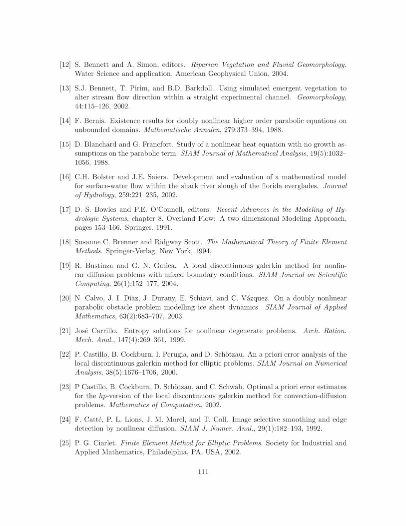
[12] S. Bennett and A. Simon, editors. Riparian Vegetation and Fluvial Geomorphology.Water Science and application. American Geophysical Union, 2004.

[13] S.J. Bennett, T. Pirim, and B.D. Barkdoll. Using simulated emergent vegetation toalter stream flow direction within a straight experimental channel. Geomorphology,44:115–126, 2002.

[14] F. Bernis. Existence results for doubly nonlinear higher order parabolic equations onunbounded domains. Mathematische Annalen, 279:373–394, 1988.

[15] D. Blanchard and G. Francfort. Study of a nonlinear heat equation with no growth as-sumptions on the parabolic term. SIAM Journal of Mathematical Analysis, 19(5):1032–1056, 1988.

[16] C.H. Bolster and J.E. Saiers. Development and evaluation of a mathematical modelfor surface-water flow within the shark river slough of the florida everglades. Journalof Hydrology, 259:221–235, 2002.

[17] D. S. Bowles and P.E. O’Connell, editors. Recent Advances in the Modeling of Hy-drologic Systems, chapter 8. Overland Flow: A two dimensional Modeling Approach,pages 153–166. Springer, 1991.

[18] Susanne C. Brenner and Ridgway Scott. The Mathematical Theory of Finite ElementMethods. Springer-Verlag, New York, 1994.

[19] R. Bustinza and G. N. Gatica. A local discontinuous galerkin method for nonlin-ear diffusion problems with mixed boundary conditions. SIAM Journal on ScientificComputing, 26(1):152–177, 2004.

[20] N. Calvo, J. I. Dıaz, J. Durany, E. Schiavi, and C. Vazquez. On a doubly nonlinearparabolic obstacle problem modelling ice sheet dynamics. SIAM Journal of AppliedMathematics, 63(2):683–707, 2003.

[21] Jose Carrillo. Entropy solutions for nonlinear degenerate problems. Arch. Ration.Mech. Anal., 147(4):269–361, 1999.

[22] P. Castillo, B. Cockburn, I. Perugia, and D. Schotzau. An a priori error analysis of thelocal discontinuous galerkin method for elliptic problems. SIAM Journal on NumericalAnalysis, 38(5):1676–1706, 2000.

[23] P Castillo, B. Cockburn, D. Schotzau, and C. Schwab. Optimal a priori error estimatesfor the hp-version of the local discontinuous galerkin method for convection-diffusionproblems. Mathematics of Computation, 2002.

[24] F. Catte, P. L. Lions, J. M. Morel, and T. Coll. Image selective smoothing and edgedetection by nonlinear diffusion. SIAM J. Numer. Anal., 29(1):182–193, 1992.

[25] P. G. Ciarlet. Finite Element Method for Elliptic Problems. Society for Industrial andApplied Mathematics, Philadelphia, PA, USA, 2002.

111

[26] B. Cockburn and C. Dawson. Some extensions of the local discontinuous galerkinmethod for convection-diffussion equations. In The Proceedings of the Conference onthe Mathematics of Finite Elements and Applications, pages 225–238. Elsevier, 2000.

[27] B. Cockburn, G. E. Karniadakis, and C. W. Shu, editors. Discontinuous GalerkinMethods. Springer, 2000.

[28] B. Cockburn and C. W. Shu. The local discontinuous galerkin method for time-dependent convection-diffusion systems. SIAM J. Numer. Anal., 35(6):2440–2463,1998.

[29] R. Courant, K. Friedrihs, and H. Lewy. Uber die partiellen differenzengleichungen dermathematischen physik. Math. Ann., 100:32–74, 1928.

[30] R. Daugherty, J. Franzini, and J. Finnemore. Fluid Mechanics with Engineering Ap-plications. McGraw-Hill, 1985.

[31] Emmanuel DiBenedetto. Degenerate Parabolic Equations. Springer-Verlag, New York,1993.

[32] J. Douglas and T.F. Dupont. Galerkin methods for parabolic equations. SIAM Journalon Numericla Analysis, 7:575–626, 1970.

[33] C. Ebmeyer and W. B. Liu. Quasi-norm interpolation error estimates for the piecewiselinear finite element approximation of p-laplacian problems. Numer. Math., 100(2):233–258, 2005.

[34] Alexandre Ern and Jean-Luc Guermond. Theory and practice of finite elements.Springer-Verlag, New York City, 2004.

[35] J.R. Esteban and J.L. Vazquez. Homogeneous diffusion in R with power-like nonlineardiffusivity. Archive Rat. Mech. Analysis, 103:39–80, 1988.

[36] Lawrence C. Evans. Partial Differential Equations. American Mathematical Society,Providence, 2002.

[37] S. Evje and K. Karlsen. Discrete approximations of bv solutions to doubly nonlineardegenerate parabolic equations.

[38] K. Feng and F.J Molz. A 2-d diffusion based, wetland flow model. Journal of Hydrology,196:230–250, 1997.

[39] P Di Giammarco, E. Todini, and P. Lamberti. A conservative finite elements approachto overland flow: the control volume finite element formulation. Journal of Hydrology,175:267–291, 1996.

[40] G. Gioia and F.A. Bombardelli. Scaling and similarity in rough channel flows. PhysicalReview Letters, 88(1), 2002.

112

[41] O. Grange and F. Mignot. Sur la resolution d’une equation et d’une inequationparaboliques non lineaires. Journal of Functional Analysis, 11:77–92, 1972.

[42] E. Hansen and A. Ostermann. Finite element runge–kutta discretizations of porousmedium–type equations. SIAM Journal on Numerical Analysis, 46(4):1769–1779, 2008.

[43] Philip Hartman. Ordinary Differential Equations. Society for Industrial and AppliedMathematics, Philadelphia, PA, USA, 2002.

[44] T.V. Hromadka, C.E. Berenbrock, J.R. Freckleton, and G.L. Guymon. A two-dimensional dam-break flood plain model. Adv. Water Resources, 8, 1985.

[45] K. Ishige. On the existence of sotutions of the cauch problem for a doubly nonlinearparabolic equation. SIAM Lournal on Mathematical Analysis, 27(5):1235–1260, 1996.

[46] Y. Iwagaki. Fundamental studies of runoff analysis by characteristics. Bulletin 10,Dis-aster Prevention Res. Inst., Kyoto University, Kyoto, Japan, 1955. 25pp.

[47] S.C. Jain. Open-channel flow. John Wiley & Sons, 2001.

[48] N. Ju. Numerical analysis of parabolic p-laplacian: Approximation of trajectories.SIAM Journal on Numerical Analysis, 37(6):1861–1884, 2000.

[49] H. Lia, M.W. Farthinga, C.N. Dawson, and C.T. Miller. Local discontinuous galerkinapproximations to richards equation. Advances in Water Resources, 30:555–575, 2007.

[50] J.L. Lions. Quelques Methodes de Resolution des Problemes aux Limites Non Lineaires.Dunod Gauthier-Villars, Paris, 1969.

[51] W. Liu and N. Yan. Quasi-norm local error estimators for p-laplacian. SIAM J. Numer.Anal., 39(1):100–127, 2001.

[52] J. Nitsche. Uber ein variationsprinzip zur losung von dirichlet-problemen bei verwen-dung von teilraumen, die keinen randbedingungen unterworfen sind. Abh. Math. Sem.Univ. Hamburg, 36, 1971.

[53] R. H. Nochetto and C. Verdi. Approximation of degenerate parabolic problems usingnumerical integration. SIAM J. Numer. Anal., 25:784 – 814, 1988.

[54] V.M. Ponce, R.M. Li, and D.B. Simons. Aplicability of kinematic and diffusion models.Journal of the Hydraulics Division, pages 353–360, 1978.

[55] V.M. Ponce and D.B. Simons. Shallow wave propagation in open channel flow. Journalof the Hydraulics Division, pages 1461–1476, 1977.

[56] P.A. Raviart. Sur la resolution de certaines equations paraboliques non lineaires. Jour-nal of Functional Analysis, 5:299–328, 1970.

[57] J. Rulla and N. J. Walkington. Optimal rates of convergence for degenerate parabolicproblems in two dimensions. SIAM Journal on Numerical Analysis, 33(1):56–67, 1996.

113

[58] M. Santillana and C. Dawson. A numerical approach to study the properties of solutionsof the diffusive wave approximation of the shallow water equations. ComputationalGeosciences, 2008. Submitted.

[59] J.W. Thomas. Numerical Partial Differential Equations: Finite Difference Methods.Number 22 in Texts in Applied Mathematics. Springer, New York, 1995.

[60] Vidar Thomee. Galerkin Finite Element Methods for Parabolic Problems. Number 25in Springer Series in Computational Mathematics. Springer, 1997.

[61] A.K. Turner and N. Chanmeesri. Shallow flow of water through non-submerged vege-tation. Agricultural Water Management, 8:375–385, 1984.

[62] J. L. Vazquez. The Porous Medium Equation. Mathematical Theory. Oxford UniversityPress, USA, 2006.

[63] C.B. Vreugdenhil. Numerical Methods for Shallow-Water Flow. Kluwer AcademicPublishers, The Netherlands, 1998.

[64] Dongming Wei and Lew Lefton. A priori Lρ error estimates for galerkin approximationsto porous medium and fast diffusion equations. Math. Comput., 68(227):971–989, 1999.

[65] T. Weiyan. Shallow Water Hydrodynamics: Mathematical Theory and Numerical Solu-tion for a Two-dimensional System of Shallow Water Equations, volume 55. Elsevier,Amsterdam, 1992.

[66] Richard L. Wheeden and Antoni Zygmund. Measure and Integral: An Introduction toReal Analysis. A series of Monographs and Textbooks. Marcel Dekker, Inc., New York,1977.

[67] M. F. Wheeler. A priori L2 error estimates for galerkin approximations to parabolicpartial differential equations. SIAM Journal on Numerical Analysis, 10(4):723–759,1973.

[68] M. F. Wheeler. An elliptic collocation finite element method with interior penalties.SIAM Journal on Numerical Analysis, 15(1):152–161, 1978.

[69] Th. Xanthopoulos and Ch. Koutitas. Numerical simulation of a two dimensional floodwave propagation due to dam failure. Journal of Hydraulic Research, 14(4):321–331,1976.

[70] J. Yan and C. W. Shu. A local discontinuous galerkin method for kdv type equations.SIAM J. Numer. Anal., 40(2):769–791, 2002.

[71] J. Yan and C. W. Shu. Local discontinuous galerkin methods for partial differentialequations with higher order derivatives. J. Sci. Comput., 17(1-4):27–47, 2002.

[72] W. Yong and I. Pop. A numerical approach to porous medium equations, 1996.

114

[73] W. Zhang and T.W. Cundy. Modeling of two-dimensional overland flow. Water Re-sources Res., 25:2019–2035, 1989.

115

Vita

Mauricio Santillana, son of Humberto Santillana Loyo and Luz Patricia Guzman Olivares,

was born on July 9th in the year 1976, in Mexico City. In 2001, he received a B.S. in

Physics with honors from the Universidad Nacional Autonoma de Mexico in Mexico City.

After which, he started graduate school at the University of Texas at Austin, earning

a M.S. in Computational and Applied Mathematics in 2003. Since 2003, he has been

part of the inter-disciplinary research team at the Research Institute for Geography and

Geomatics, CentroGeo, based in Mexico City and part of the National Council for Science

and Technology of Mexico. In 2004, Mauricio started his Ph.D. studies at the Institute for

Computational Engineering and Sciences at the University of Texas at Austin.

Permanent Address: 3914 Avenue HAustin, TX 78751

This dissertation was typeset with LATEX2ε1 by the author.

1LATEX2ε is an extension of LATEX. LATEX is a collection of macros for TEX. TEX is a trademark of theAmerican Mathematical Society. The macros used in formatting this dissertation were written by DineshDas, Department of Computer Sciences, The University of Texas at Austin, and extended by Bert Kay,James A. Bednar, and Ayman El-Khashab.

116