Copyright by Malek Mohamed Lemkecher 2009

Copyright

by

Malek Mohamed Lemkecher

2009

INTERACTIVE INTERPRETATION OF NUCLEAR LOGS

WITH FAST MODELING PROCEDURES

by

MALEK MOHAMED LEMKECHER, B. S.

THESIS

Presented to the Faculty of the Graduate School of

The University of Texas at Austin

in Partial Fulfillment

of the Requirements

for the Degree of

MASTER OF SCIENCE IN ENGINEERING

The University of Texas at Austin

December 2009



APPROVED BY SUPERVISING COMMITTEE:

Carlos Torres-Verdín, Supervisor

William E. Preeg, Co-Supervisor

DEDICATION

First and foremost, I dedicate this thesis to our God the Merciful, who has continuously

guided me in all my motivations.

Then I dedicate the work presented in this thesis to my parents Boubaker and Bakhta,

my brother Khalil, and my sister Emna for their unconditional and unique love.

Thanks to you all for supporting me throughout untold periods of time working on this

research.

v

ACKNOWLEDGEMENTS

I am extremely thankful to my supervisor, Dr. Carlos Torres-Verdín for his

outstanding pedagogy, valuable advice and consistent support during the preparation of

this research project. I hope he will be proud of me throughout future successful

challenges in my career. I also express my gratitude and special thanks to Dr. William E.

Preeg for graciously accepting to be the second reader of this thesis. I thank the fellows in

our research group – in particular Ben Voss, Alberto Mendoza, Amir Reza Rahmani

Zoya Heidari, and Jorge Sanchez – for their collaboration in the development of this

project.

The work reported in this thesis was partially funded by The University of Texas

at Austin’s Research Consortium on Formation Evaluation, jointly sponsored by

Anadarko, Aramco, Baker-Hughes, BHP Billiton, BP, BG, Chevron, ConocoPhillips,

ENI, ExxonMobil, Halliburton, Hess, Marathon, Mexican Institute for Petroleum, Nexen,

Petrobras, RWE, Schlumberger, Statoil Hydro, TOTAL, and Weatherford.

Malek Mohamed Lemkecher

Austin, TX December 2009

vi

ABSTRACT



Malek Mohamed Lemkecher, M.S.E.

The University of Texas at Austin, 2009

Supervisor: Carlos Torres-Verdín

This thesis introduces new software to interactively construct multi-layer models

and bedding sequences, populate layer-by-layer properties, and enable the fast simulation

of nuclear logs. The method consists of modifying simultaneously layer thicknesses and

properties to rapidly simulate the outcome (nuclear logs) for comparison to field logs. I

include applications which appraise the numerical simulation of gamma-ray, density,

compensated neutron, and photoelectric factor logs. An analogous application for sonic

modeling is considered as well which uses a modified version of Wyllie’s slowness

averaging equation. The procedure is tested for the case of vertical wells and horizontal

layers. Examples of application include 6 synthetic and 5 field examples. Additionally,

the software is implemented in combination with other formation-evaluation procedures

vii

to interpret resistivity and nuclear logs. Simulations of nuclear logs for synthetic models

can be used to improve the assessment and interpretation of field data.

Interactive modeling and simulation of nuclear logs provides a very good

agreement with field logs with an average error of 3.9%. The order of logs to be matched

as well as the data available are significant factors in the accuracy of the match.

Numerical simulation and matching of field logs using fast modeling procedures is a

reliable method to improve the inference of static and dynamic petrophysical properties

of rock formations.

viii

TABLE OF CONTENTS

Acknowledgments ..................................................................................................v

Abstract................................................................................................................. vi

Table of Contents ............................................................................................... viii

List of Tables ........................................................................................................ xi

List of Figures...................................................................................................... xii

Chapter 1 Introduction.........................................................................................1

1.1 Background ..............................................................................................1

1.2 Purpose......................................................................................................1

1.3 Organization of this Thesis .......................................................................5

Chapter 2 Bed Properties Tool ............................................................................7

2.1 Functionality ............................................................................................7

2.2 Outline.......................................................................................................8

2.2.1 Matrix .........................................................................................10

2.2.2 Fluid/Gas ....................................................................................10

2.2.3 Shale ...........................................................................................10

2.2.4 Common Petrophysical/Fluid Properties ...................................11

2.3 Component Properties.............................................................................11

2.4 Data Treatment........................................................................................15

Chapter 3 Simulation of Borehole Nuclear Measurements ............................17

3.1 Description of the module ......................................................................17

3.2 Functionality ...........................................................................................18

Chapter 4 Case Studies.......................................................................................21

4.1 Synthetic case .........................................................................................21

4.1.1 Changing the fluid composition .................................................22

4.1.2 Including an additional layer .....................................................24

4.1.3 Modifying porosity ....................................................................25

ix

4.1.4 Including an additional mineral in the bulk solid composition ..26

4.1.5 Adding thinly-bedded layers ......................................................27

4.1.6 Salinity effect on nuclear logs ....................................................28

4.2 Field Studies ...........................................................................................30

4.2.1 Carbonate Formation .................................................................30

4.2.2 Siliciclastic Formation ...............................................................34

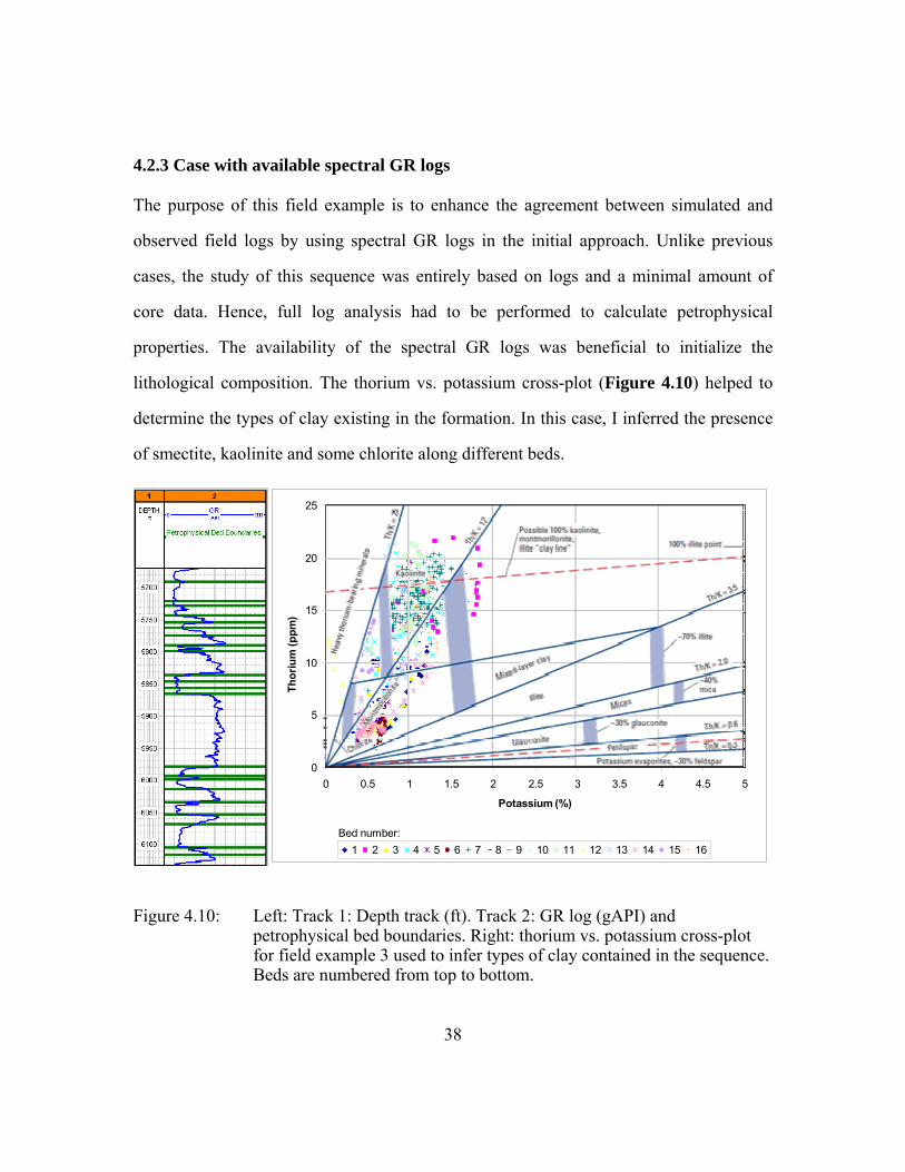
4.2.3 Case with available spectral GR logs..........................................38

4.2.4 Case with an illustrated manually-iterated procedure ................42

4.2.5 Offshore Formation ....................................................................47

Chapter 5 Summary and Conclusions ..............................................................50

5.1 Summary ................................................................................................50

5.2 Conclusions.............................................................................................50

x

Appendix A...........................................................................................................53

Detailed Inventory of Well-Logs Available for the Field Cases ......................53

Appendix B ...........................................................................................................54

Archie's Equation and Summary of Parameters Considered For the Modeling of Water Saturation Curves ...........................................................................54

Appendix C...........................................................................................................55

Dual-Water Equation and Summary of Parameters Considered For the Modeling of Water Saturation Curves......................................................55

Nomenclature .......................................................................................................56

References.............................................................................................................59

Vita ......................................................................................................................61

xi

List of Tables

Table 2.1: Summary of solid properties defaulted in the Palette. Values can be

customized based on specific field characteristics............................12

Table 2.2: Summary of fluid properties defaulted in the Palette. Complex fluid

values cannot be modified since each property is unique for each

element..............................................................................................13

Table A.1: Detailed inventory of well logs available for this study. ..................52

xii

List of Figures

Figure 1.1: Objective of the thesis represented in flow-chart relations that emphasize

the connection between the lithological/fluid composition and numerical

simulation of logs................................................................................4

Figure 1.2: Generic flowchart of UT Petrophysical and Well-Log Simulator,

emphasizing the role of this thesis. .....................................................5

Figure 2.1: Flow chart describing two options which can be defined for simulation

of nuclear logs. Input data can be either user-defined beds, or raw field

data. In the former case, the manual iterative procedure is identified with

a dashed line........................................................................................8

Figure 2.2: Snapshot of the selection palette. Each section is highlighted with a

different color. The user enters his/her own definition for each

boundary-defined bed. This step is accessible again if the user wishes to

make modifications following the simulation results. Once nuclear

properties have been defined for each bed, the user can perform

numerical simulations. The Common Petrophysical/Fluid Properties

section allows the user to enter the temperature gradient in the absence

of a temperature log, shale structure, and water salinity.....................9

Figure 2.3a: Snapshot of the Solid Component Properties. Each component is

associated with its own defined chemical formula, density, spectral

gamma-ray values, and acoustic transient time. ...............................14

xiii

Figure 2.3b: Snapshot of the Generic Fluid Component Properties. Each component

is associated with its defined chemical formula, acoustic transient time,

critical pressure and temperature, acentric factor, and molecular weight.

...........................................................................................................14

Figure 3.1: Snapshot of the Nuclear Logs Simulator. Based on the selected

simulation types, different options will be enabled/disabled for log

calculations. ......................................................................................18

Figure 3.2: Example of Density (limestone porosity units) vs. Neutron (limestone

porosity units) cross-plot distinctly colored for each layer...............20

Figure 4.1: Description of the synthetic model with corresponding simulated logs.

Track 0: Lithology log: Limestone (green), Shale (orange), Sandstone

(yellow), and Dolomite (blue). Track 1: Bed boundaries and

environmentally corrected gamma-ray simulated log (ECGR, gAPI).

Track 2: Simulated neutron (NPHI, limestone porosity units) and density

logs (ρα, g/cm3). Track 3: PEF simulated log (barn/electron) and sonic

slowness log (VP,formation, μs/ft). Track 4: Depth track (ft). ...............22

Figure 4.2: Simulated logs for the synthetic model with 90% of methane in fluid

saturations. Track 0: Lithology log: Limestone (green), Shale (orange),

Sandstone (yellow), and Dolomite (blue). Track 1: Bed boundaries and





xiv

Figure 4.3: Simulated logs for the synthetic model with an additional layer of

anhydrite. Track 0: Lithology log: Limestone (green), Shale (orange),

Sandstone (yellow), Dolomite (blue), and Anhydrite (red). Track 1: Bed

boundaries and environmentally corrected gamma-ray simulated log

(ECGR, gAPI). Track 2: Simulated neutron (NPHI, limestone porosity

units) and density logs (ρα, g/cm3). Track 3: PEF simulated log

(barn/electron) and sonic slowness log (VP,formation, μs/ft). Track 4: Depth

track (ft). ...........................................................................................24

Figure 4.4: Simulated logs for the synthetic model after modifying the overall

porosity. Track 0: Lithology log: Limestone (green), Shale (orange),






Figure 4.5: Simulated log of the synthetic model with a modified matrix

composition. Track 0: Lithology log: Limestone (green), Shale (orange),






xv

Figure 4.6: Simulated logs for the synthetic model with a sequence of thin beds of

sand and shale. Track 0: Lithology log: Limestone (green), Shale

(orange), Sandstone (yellow), Dolomite (blue), and a sequence of thin

beds of shale and sand (brown). Track 1: Bed boundaries and





Figure 4.7: Simulated logs for a synthetic case with a sequence of limestone beds of

equal petrophysical properties but different salinities. Track 1: Bed

boundaries, migration length (Lmformation, ft), and PEF (barns/electron)

logs. Track 2: Simulated neutron (NPHI, limestone porosity units) and

density logs (ρα, g/cm3). Track 3: Volumetric concentration of NaCl in

connate water (Cw, ppm). ..................................................................29

Figure 4.8a: Field and simulated logs for the carbonate example. Track 1: Depth

track (ft). Track 2: Bed boundaries and caliper (ft). Track 3: Lithology

(fraction): orthoclase (grey), quartz (yellow), biotite (green), dolomite

(purple), limestone (black), glauconite (orange), illite (gold), water

(blue), shale water (light blue), oil (red). Track 4: GR (gAPI). Track 5:

Density (g/cm3). Track 6: Neutron (limestone porosity units). Track 7:

Sonic slowness (μs/ft). Track 8: PEF (barn/electron). ......................31

xvi

Figure 4.8b: Field and simulated logs for the carbonate example. Track 1: Depth


(fraction): orthoclase (grey), quartz (yellow), biotite (green), dolomite

(purple), limestone (black), glauconite (orange), illite (gold), water

(blue), shale water (light blue), oil (red). Tracks 4 to 8: High-Resolution

Laterolog Array Tool from shallow to deeper depths of investigation

(Ω.m).................................................................................................32

Figure 4.8c: Spatial distribution of resistivity and water saturation. Track 1: Depth

track (ft). Track 2: Lithology (fraction): orthoclase (grey), quartz

(yellow), biotite (green), dolomite (purple), limestone (black), glauconite

(orange), illite (gold), water (blue), shale water (light blue), oil (red).

Track 3: GR (gAPI). Track 4: High-Resolution Laterolog Array Tool

(Ω.m). Track 5: Water saturation (fraction)......................................33

Figure 4.9a: Lithology log used as the starting point for the assessment of lithology

and petrophysical properties of layers. Left column represents the user-

defined layers. Track 1: Bulk mineral composition. Track 2: Fluid

composition.......................................................................................36

Figure 4.9b: Field and simulated logs for the siliciclastic example. Track 1: Depth


(fraction): quartz (yellow), limestone (red), illite (grey), water (blue),

shale water (light blue). Track 4: GR (gAPI). Track 5: Density (g/cm3).

Track 6: Neutron (sandstone porosity units). Track 7: PEF

(barn/electron). Track 8: Sonic slowness (μs/ft)...............................37

xvii

Figure 4.10: Left: Track 1: Depth track (ft). Track 2: GR log (gAPI) and

petrophysical bed boundaries. Right: thorium vs. potassium cross-plot

for field example 3 used to infer types of clay contained in the sequence.

Beds are numbered from top to bottom. ...........................................38

Figure 4.11a: Field and simulated logs for example No. 3. Track 1: Depth track (ft).

Track 2: Bed boundaries and caliper (ft). Track 3: Lithology (fraction):

quartz (yellow), smectite (grey), kaolinite (brown), illite (purple), shale

water (dark blue), water (blue), hydrocarbon (red). Track 4: GR (gAPI).

Track 5: thorium concentration (ppm). Track 6: uranium concentration

(ppm). Track 7: potassium concentration (%). Track 8: Raw Spherically

Focused Conductivity (Ω.m).............................................................40

Figure 4.11b:Field and simulated logs for example No. 3. Track 1: Depth track (ft).

Track 2: Bed boundaries and caliper (ft). Track 3: Lithology (fraction):

quartz (yellow), smectite (grey), kaolinite (brown), illite (purple), shale

water (dark blue), water (blue), hydrocarbon (red). Track 4: GR (gAPI).

Track 9: Density (g/cm3). Track 10: Neutron (sandstone porosity units).

Track 11: Sonic slowness (μs/ft).......................................................41

Figure 4.12a:Field example No. 4: First iteration based on the carbonate assumption.

Track1: Depth track (ft). Track 2: Caliper (ft) and bed boundaries. Track

3: Field and simulated GR logs (gAPI). Track 5: Neutron (limestone

porosity units) and Density (g/cm3) field logs, water (green) and

hydrocarbon cross-over (yellow). Track 6: Neutron (limestone porosity

units) and Density (g/cm3) simulated logs, water (green) and

hydrocarbon cross-over (yellow). .....................................................43

xviii

Figure 4.12b: Second iteration applied on the previous model. Track1: Depth track

(ft). Track 2: Caliper (ft) and bed boundaries. Track 3: Field and

simulated GR logs (gAPI). Track 4: Neutron (sandstone porosity units)

and Density (g/cm3) field logs, water (green) and hydrocarbon cross-

over (yellow). Track 5: Neutron (limestone porosity units) and Density

(g/cm3) simulated logs, water (green) and hydrocarbon cross-over

(yellow). Track 6: Sonic slowness (μs/ft). ........................................45

Figure 4.13: Final model after the introduction of the resistivity log. Track1: Depth

track (ft). Track 2: Caliper (ft), bed boundaries, and petrophysical bed

boundaries. Track 3: Field and simulated GR logs (gAPI). Track 4: Field

and simulated Neutron (sandstone porosity units) logs. Track 6: Field

and simulated Density (g/cm3) logs. Track 7: Sonic slowness (μs/ft).

Track 8: Neutron (sandstone porosity units) and Density (g/cm3) field

logs, water (green) and hydrocarbon cross-over (yellow). Track 9:

Neutron (limestone porosity units) and Density (g/cm3) simulated logs,

water (green) and hydrocarbon cross-over (yellow). ........................46

Figure 4.14a: Field and simulated logs for the offshore formation. Track 1: Bed

boundaries, petrophysical bed boundaries and caliper (ft). Track 2:

Lithology (fraction): quartz (yellow), biotite (brown), orthoclase (green),

illite (grey), chlorite (pink), glauconite (dark green), shale water (dark

blue), water (blue), oil (red). Track 3: GR (gAPI). Track 4: Density

(g/cm3). Track 5: Neutron (sandstone porosity units). Track 6: Depth

track (ft) ............................................................................................48

xix

Figure 4.14b: Field and simulated logs for the offshore formation. Track 1: Bed

boundaries, petrophysical bed boundaries and caliper (ft). Track 2:

Lithology (fraction): quartz (yellow), biotite (brown), orthoclase (green),

illite (grey), chlorite (pink), glauconite (dark green), shale water (dark

blue), water (blue), oil (red). Tracks 6 to 10: Array Induction Two Foot

Resistivity Tool from shallow to deeper depths of investigation (Ω.m).

...........................................................................................................49

1

CHAPTER 1

INTRODUCTION

1.1 BACKGROUND

There are four major borehole nuclear measurements: Gamma-Ray (GR),

Density, Neutron, and Photoelectric Factor (PEF). While GR and PEF primarily respond

to the solid components of a rock, density and neutron logs respond to the fluid that is

contained within the rock’s pore space, as well as to the solid (matrix) component.

Furthermore, the GR log measures natural radioactivity, whereas the remaining three

measurements are acquired with a radioactive source.

Ellis et al. (2003) proposed a design of thermal neutron tools that reveals the

sensitivity of the measurements to both porosity and slowing-down length of the

formation. This study has been generalized in a subsequent publication of Ellis et al.

(2004) to cover the sensitivity of the same measurements to lithology, gas saturation, and

presence of shale.

In order to quantify porosity and matrix lithology effects on the depth of

investigation of neutron and density tools, Sherman and Locke (1975) described

experimental work to study invasion effects on a formation saturated with salt water by

varying fluids across different levels of invasion. Wiley and Patchett (1994) approached

the problems of invasion and differences in radial length of investigation using a

deterministic diffusion code to model thermal neutron and porosity measurements with

different formations. Furthermore, Tittle (1992) employed an analytical version of the

diffusion theory to quantify the effect of invasion on nuclear measurements for different

2

radial lengths of invasion. Such simulations considered both sources and sensors as

infinitesimal objects.

Watson (1984) introduced the concept on Monte Carlo-derived differential

sensitivity functions for detector responses due to Compton and photoelectric gamma-ray

interactions. This concept led to fast nuclear log simulation with the use of linear

sensitivity functions. Afterward, Aristodemou et al. (2006) developed a method to

diminish the computational time needed in the simulation of well-logging nuclear

measurements using the energy group optimization theory.

In an earlier work, Radtke et al. (2007) showed that the resolution of density and

neutron logs is governed by the source-to-detector distance. Several methods have been

investigated, notably the Monte Carlo N-Particle (X-5 Monte Carlo Team MCNP, 2003)

code, to simulate borehole nuclear measurements.

Mendoza et al. (2007) developed fast approximate numerical procedures making

use of Monte Carlo-derived spatial flux-scattering functions (FSFs) for specific tool

configurations, which have been used in this thesis.

Wyllie et al. (1956) proposed an averaging equation for sonic slowness. In this

thesis, we adapt this equation to make it relevant for both siliciclastic and carbonate

sequences.

1.2 PURPOSE

The main objective of this thesis is to allow the user to match field logs with

numerical simulations by interactively modifying geometrical and petrophysical

properties of layers. Figure 1.1 describes this objective in flow-chart relations that

emphasize the connection between the lithological/fluid composition and the numerical

simulation of logs.

3

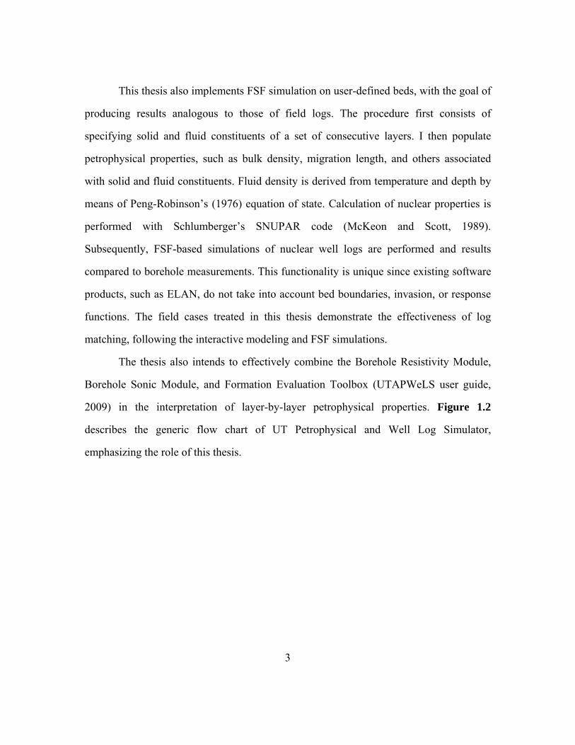
This thesis also implements FSF simulation on user-defined beds, with the goal of

producing results analogous to those of field logs. The procedure first consists of

specifying solid and fluid constituents of a set of consecutive layers. I then populate

petrophysical properties, such as bulk density, migration length, and others associated

with solid and fluid constituents. Fluid density is derived from temperature and depth by

means of Peng-Robinson’s (1976) equation of state. Calculation of nuclear properties is

performed with Schlumberger’s SNUPAR code (McKeon and Scott, 1989).

Subsequently, FSF-based simulations of nuclear well logs are performed and results

compared to borehole measurements. This functionality is unique since existing software

products, such as ELAN, do not take into account bed boundaries, invasion, or response

functions. The field cases treated in this thesis demonstrate the effectiveness of log

matching, following the interactive modeling and FSF simulations.

The thesis also intends to effectively combine the Borehole Resistivity Module,

Borehole Sonic Module, and Formation Evaluation Toolbox (UTAPWeLS user guide,

2009) in the interpretation of layer-by-layer petrophysical properties. Figure 1.2

describes the generic flow chart of UT Petrophysical and Well Log Simulator,

emphasizing the role of this thesis.

Nuclear

Electrical

Acoustics

Simulated logs match to field logsFluid Type

Porosity

Mineral Type

Con

stituents/C

ompo

sition

Num

erica

l Sim

ula

tionDensity

Gamma-ray

Neutron

PEF

Resistivity

Sonic

Nuclear

Electrical

Acoustics

Simulated logs match to field logsFluid Type

Porosity

Mineral Type

Con

stituents/C

ompo

sition

Num

erica

l Sim

ula

tionDensity

Gamma-ray

Neutron

PEF

Resistivity

Sonic

Figure 1.1: Objective of the thesis represented in flow-chart relations that emphasize the connection between the lithological/fluid composition and numerical simulation of logs.

4

SonicModule

ResistivityModule

InvasionModule

Formation Testing Module

Log ASCII Standard extraction

Sim

ula

tion

Bed

-Bo

un

dary

Defin

ition

Monte Carlo N_Particle input

Simulated logs Match Field Logs?

No

Yes

Spectral Gamma-ray

Density&

PEF

Neutron

Plo

tC

om

mo

n E

arth

Mo

del

a, b, ccoeffs

UTAPWeLS

Nuclear Module

SonicModule

ResistivityModule

InvasionModule

Formation Testing Module

Log ASCII Standard extraction

Sim

ula

tion

Bed

-Bo

un

dary

Defin

ition

Monte Carlo N_Particle input

Simulated logs Match Field Logs?

No

Yes

Spectral Gamma-ray

Density&

PEF

Neutron

Plo

tC

om

mo

n E

arth

Mo

del

a, b, ccoeffs

UTAPWeLS

Nuclear Module

Figure 1.2: Generic flowchart of UT Petrophysical and Well-Log Simulator, emphasizing the role of this thesis.

1.3 ORGANIZATION OF THIS THESIS

This thesis is organized as follows:

Chapter 2 details the characteristics of the Bed Properties Tool introduced in the

thesis. It also describes the modeling algorithm, as well as the computations behind it.

Chapter 3 details the characteristics of the Nuclear Simulation Module that

follows the modeling of the beds, consisting of FSF-based simulations and the options

included with them.

5

6

Chapter 4 analyzes the results of several synthetic and field case studies. These

cases contain different situations encountered in practice, such as carbonate, siliciclastic,

and thinly-bedded formations. Different methods are considered in order to establish the

final assessments, emphasizing the manual iterative procedure used to match field logs,

full log analysis, and initial guess.

Chapter 5 summarizes the most important conclusions stemming from the

modeling and simulation exercises.

7

CHAPTER 2

BED PROPERTIES TOOL

This chapter provides a detailed description of the Bed Properties tool used for the

modeling of horizontal beds, as well as of the computations behind the modeling

algorithm.

2.1 FUNCTIONALITY

The Bed Properties tool is a set of interfaces used to facilitate the lithological

description of a chosen bed sequence, as well as some of its petrophysical properties.

This description can be specifically defined for different beds within the same sequence,

as well as its fluid properties, which may change radially. Once the sequence has been

defined, a final interface allows the user to simulate the proposed definition in order to

compare it to the corresponding field logs. This process will be then repeated in order to

refine the result (Figure 2.1).

The definition of bed boundaries can be either done arbitrarily or using the Master

Curve Selection tool that permits the user to designate a field log in order to simulate it.

This generation may be performed by squaring the designated log (gamma-ray log for

example) and setting a shale index value limit so that it separates sands from shales for

the case of siliciclastic sequences.

Bed Boundaries

Definition

Palette

BoreholeNuclearModule

Plot&

Display

LAS

Master Curve

Selection

Log Squaring

Nuclear Properties

•Solid components•Fluid components •Shale components

Nuclear Logs

Designated Logs

SimulatedLogs

User

Good Match to

Log Data?

END

START

Yes

No

Snupar

LmBed

Boundaries Definition

Palette

BoreholeNuclearModule

Plot&

Display

LAS

Master Curve

Selection

Log Squaring

Nuclear Properties

•Solid components•Fluid components •Shale components

Nuclear Logs

Designated Logs

SimulatedLogs

User

Good Match to

Log Data?

END

START

Yes

No

Snupar

Lm

Figure 2.1: Flow chart describing two options which can be defined for simulation of nuclear logs. Input data can be either user-defined beds, or raw field data. In the former case, the manual iterative procedure is identified with a dashed line.

The manual iteration process can be performed at two levels: either by returning

to the bed-boundary definition in order to add more layers or split a previously defined

layer, or by reviewing the bed-property definition at the palette level (Figure 2.2). In

either case, nuclear simulations have to be performed once more to quantify the resulting

changes, and improve the match to field logs.

2.2 OUTLINE

Bed properties are defined with a selection palette that allows the user to assign

different parameters to each consecutive bed. These attributes are classified into

components: Matrix, Fluid, Shale, and Common Petrophysical/Fluid properties (Figure

2.2).

8

Figure 2.2: Snapshot of the selection palette. Each section is highlighted with a different color. The user enters his/her own definition for each boundary-defined bed. This step is accessible again if the user wishes to make modifications following the simulation results. Once nuclear properties have been defined for each bed, the user can perform numerical simulations. The Common Petrophysical/Fluid Properties section allows the user to enter the temperature gradient in the absence of a temperature log, shale structure, and water salinity.

9

10

2.2.1 Matrix

The matrix selection permits the user to enter different combinations of each solid

matrix component of a bed based upon mineral constituents. Minerals vary from mica,

calcite, etc. After the minerals are entered, the software checks whether their respective

fractions add up to one, thereby verifying that the user has entered all the specific

constituents.

2.2.2 Fluid/Gas

The fluid selection allows the user to input different combinations of fluid/gas

contained in the rock’s pore space. Constituents can be fresh water, brine, and/or

hydrocarbon. Hydrocarbons predefined in the software range from methane (CH4) to

Eikosane (C20H42). All isomers are included since their densities vary as well. Similar to

the solid selection when the user validates their entry, the software verifies whether the

sum of the fluid saturations adds up to one. Since brine is a generic term for saline water,

the user can specify its salt concentration in order to readjust the corresponding fluid

density.

2.2.3 Shale

The shale selection permits users to enter both the solid and fluid components of

any type of shale. The solid part of the shale is generally silt (quartz) and clay, while the

fluid part can be anything previously mentioned in the main fluid selection. Users also

enter the porosity of the shale such that the corresponding molecular properties are

properly weighted.

11

2.2.4 Common Petrophysical/Fluid Properties

The last section contains all other relevant definitions related to any chosen bed.

Non-shale porosity and volumetric shale concentration are required to ensure the

accuracy of the calculations undertaken by the software. Temperature is necessary for the

simulation of density and neutron measurements, and can be either entered manually,

selected from a field log (if available), or calculated from two different depths with their

corresponding temperature values. Salinity may be required if the connate water

saturation is considerably high, and can be entered either in NaCl, KCl, or CaCl2

volumetric concentrations (ppm). If one of the two latter options is used, it will get

automatically converted to NaCl salinity based on a coefficient chart.

2.3 COMPONENT PROPERTIES

A detailed data base of pure mineral properties is required to simulate gamma-ray

and sonic logs. Tables 2.1 and 2.2 describe the set of parameters used in most of the

cases discussed in this thesis (Mineral Mnemonics, SIS). The data base has been

separated into solid and fluid composition since the nature of its respective properties is

different. Furthermore, the fluid data set exists in both generic mode (common

definitions) and specific mode where one can attribute properties to distinct chemical

formulas. Knowing that these values may vary slightly due to packing and diagenesis,

one may have to adjust the minerals and their volumetric concentration in order to

improve the simulation results. This can be done in the Solid Component Properties

(Figure 2.3a) and the Generic Fluid Component Properties (Figure 2.3b).

12

Name Chemical formula Density (ρ, g/cc)

Potassium(K, %)

Uranium (U, ppm)

Thorium (Th, ppm)

Sonic slowness(Δt, μs/ft)

Silicates Quartz SiO2 2.64 0.073 0.1 0.2 55.6Orthoclase KAlSi3O8 2.52 12.9 0.005 0 69Plagioclase NaAlSi3O8 2.69 0.54 0.005 0 69Micas Biotite KMg2.5Fe0.5AlSi3O10O1.75H1.75F0.25 3.1 7.5 0.005 0 50Muscovite KAl2Si3O10O1.8H1.8 2.82 8.85 0.005 0 49Carbonates Dolomite CaMgCO3 2.85 0.2 1 5.75 43.5Limestone (Calcite) CaCO3 2.71 0.05 0.25 0.5 47.6Siderite FeCO3 3.89 0 0 0 47Anhydrite CaSO4 2.98 0 0 0 50Gypsum CaSO4H4O2 2.32 0 0 0 52.6Clays Kaolinite Al4Si4O10O8H8 2.41 0.42 12.5 2.25 -Illite K1.25Al4Si6.75Al1.25O20O4H4 2.52 4.5 0 1.5 -Smectite Ca7Na7Al4Mg4Fe4Si8Al8O20O4H4H2O 2.12 0.16 19 3.5 -Vermiculite Mg1.8Fe0.9Al4.3SiO10O2H2H8O4 2.5 0 0 0 -Bentonite Al2O3Si4O8H8O4 2.6 0.25 28 9.5 -Glauconite K0.7MgFe2AlSi4Al10O2OH 2.86 5.19 0 0 -Chlorite Mg6Fe6Al6Si4Al4O10O8H8 2.76 0 0 0 -Evaporites Halite (Salt) NaCl 2.35 0 0 0 66.7

Sulfur S 2.07 0 0 0 -

Table 2.1: Summary of solid properties defaulted in the Palette. Values can be customized based on specific field characteristics.

13

Name Chemical formula

Sonic slowness (Δt, μs/ft)

Critical pressure (Pc , atm)

Critical temperature

(Tc , K)

Acentric factor

(ω)

Molecular weight

(M, g/mol) Generic Fluids Water H2O 218 217.6 647.3 0.344 18.015Sour Gas H2S 626 88.2 373.2 0.1 34.08Light Gas CH4 626 45.35 190.45 0.008 16.04Gas C3H8 626 41.25 352.09 0.1404 44.0964Light Oil C7H16 293.429 32.2571 547.771 0.315 95.8964Oil C14H30 238 19.1956 696.711 0.608341 192.367Paraffin Wax C31H64 238 9.925 883.023 1.11268 415.462Complex Fluids C4H10 C4H10 626 37.5 425.2 0.193 58.124C10H22 C10H22 238 20.8 617 0.49 142.3C20H42 C20H42 238 14.36 782.9 0.816053 275C30H62 C30H62 238 10.12 872.5 1.082281 394

C45H92 C45H92 238 7.14 957.8 1.329531 539

Table 2.2: Summary of fluid properties defaulted in the Palette. Complex fluid values cannot be modified since each property is unique for each element.

Figure 2.3a: Snapshot of the Solid Component Properties. Each component is associated with its own defined chemical formula, density, spectral gamma-ray values, and acoustic transient time.

Figure 2.3b: Snapshot of the Generic Fluid Component Properties. Each component is associated with its defined chemical formula, acoustic transient time, critical pressure and temperature, acentric factor, and molecular weight.

14

2.4 DATA TREATMENT

After the software checks for input errors, the user has a valid input for a given

bed. For the case of gamma-ray measurements, the software recalls from a data base the

radioactivity proportion for each mineral input. Radioactivity is measured in parts-per-

million (ppm) of Uranium and Thorium, and fraction (%) of Potassium. Amounts are re-

evaluated after adding the values from the Solid Components of the Shale selection. In

addition to the solid data base, the software uses a data base that contains four properties

for each fluid/gas: critical pressure (Pc), critical temperature (Tc), acentric factor (ω), and

molecular weight (M). These four properties, in addition to bed temperature and bed

pressure, are necessary to calculate the corresponding fluid density using Peng-

Robinson’s method. Bed pressure is assumed to be equivalent to the hydrostatic pressure

at a particular depth. Once the fluid/gas densities are retrieved, the software scales the

density based on the rock’s composition and calculates the corresponding neutron

migration length (via SNUPAR). These two parameters, in addition to the previously

averaged radioactivity spectral values, are finally stored for access by the second part of

the software where numerical simulations take place.

Apart from the data to be used for nuclear simulation, the Palette includes a sonic

P-wave slowness model. Similarly to density weighted averaging, this model is generated

by combining each bed’s composition. We use Wyllie’s (1956) averaging equation for

this purpose:

1 1

b ft t ts

, (2.1)

where is porosity (fraction) and Δt is sonic slowness (time per distance) of the pure

bulk, fluid, and solid (Δtb, Δtf, and Δts, respectively). Since we will be dealing with both

siliciclastic and carbonate sequences, we adapted Wyllie’s equation to read as

15

])1([)1( ,, sshshfshshshsshfb ttCtCtt , (2.2)

where the subscripts “sh,f” and “sh,s” designate the shale fluid and solid properties,

respectively, and Csh is the corresponding volumetric concentration.

16

17

CHAPTER 3

SIMULATION OF BOREHOLE NUCLEAR MEASUREMENTS

This chapter describes the characteristics of the Nuclear Simulation Module,

which comes into play after beds have been defined. These simulations are FSF-based

and can be adjusted with certain options.

3.1 DESCRIPTION OF THE MODULE

The Borehole Nuclear Module is a user-friendly graphical interface for the

simulation and interpretation of nuclear measurements (Figure 3.1). These measurements

are performed based on the data previously generated by the Palette. Numerical modeling

is based on iterative, linear-refinement approximations (Mendoza, 2009).

Figure 3.1: Snapshot of the Nuclear Logs Simulator. Based on the selected simulation

types, different options will be enabled/disabled for log calculations.

3.2 FUNCTIONALITY

Simulations performed by this module concern GR, density, compensated

neutron, and PEF. Specifically, GR simulation is performed from the Thorium, Uranium

and Potassium concentrations. Compensated neutron logs are simulated from migration

lengths. For the case of simulation of density and PEF measurements, we choose density

of the formation as the weighted nuclear sensitivity parameter. All these parameters are

related to the cross-section and therefore to the tool response (count rate).

18

Prior to performing the GR simulation, the three spectral models are weighted for

each separate bed using the formula

KcUbThaGR ccc , (3.1)

where GR is the weighted gamma ray value (gAPI); Th and U are the thorium and

uranium concentration (part per million), respectively; K is the potassium concentration

(%); and ac, bc, and cc are their corresponding coefficients, which are defaulted to be

2.71, 6.51, and 14.23, respectively. These values may differ based on the formation, but

are constant within the same sequence. Once the weighted GR value is obtained, FSF-

based simulations are performed by the module (Mendoza et al., 2007).

Among the options available for density and compensated neutron simulations,

the user can refine the results by adding a linear iterative refinement, which takes into

account the FSF spatial variations. This refinement takes into account the variations of

the response functions that are due to local perturbations of energy-dependent cross-

section (Mendoza, 2009). This option, on the other hand, will increase the Central

Processing Unit (CPU) time of the simulations.

Based on the type of simulation selected, certain cross-plots will be available for

display. They consist of Density vs. Neutron (Figure 3.2), Potassium vs. Thorium, PEF

vs. Th/K, and PEF vs. Density. Each cross-plot is overlaid by its corresponding

interpretation chart (Log Interpretation Charts, SIS), which helps the user to diagnose and

verify the model lithology.

19

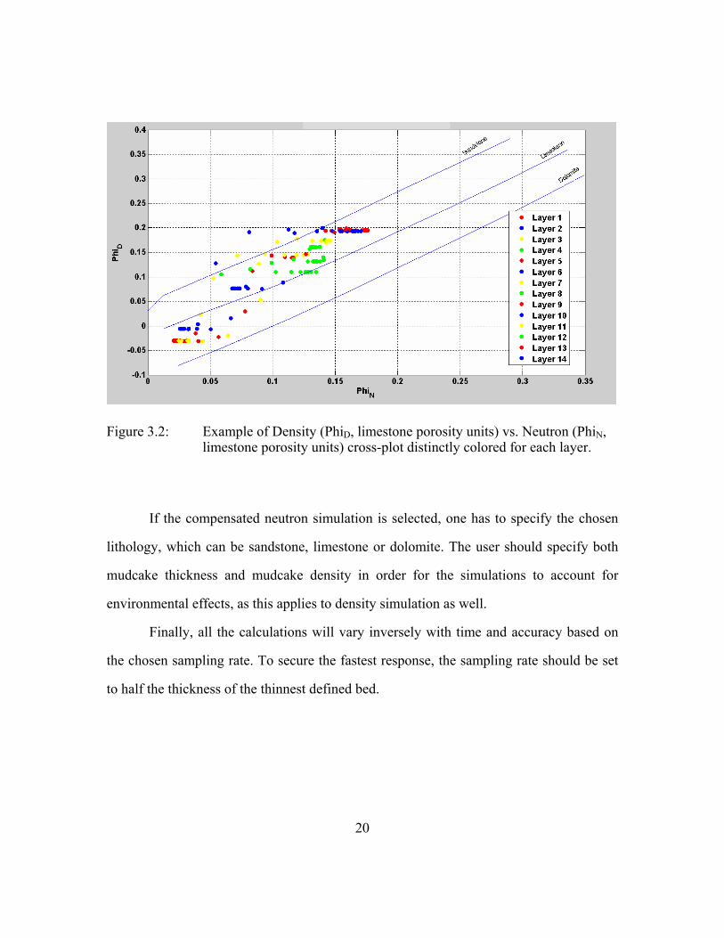
Figure 3.2: Example of Density (PhiD, limestone porosity units) vs. Neutron (PhiN, limestone porosity units) cross-plot distinctly colored for each layer.

If the compensated neutron simulation is selected, one has to specify the chosen

lithology, which can be sandstone, limestone or dolomite. The user should specify both

mudcake thickness and mudcake density in order for the simulations to account for

environmental effects, as this applies to density simulation as well.

Finally, all the calculations will vary inversely with time and accuracy based on

the chosen sampling rate. To secure the fastest response, the sampling rate should be set

to half the thickness of the thinnest defined bed.

20

21

CHAPTER 4

CASE STUDIES

This chapter evaluates the previously defined methods on several case studies,

including both synthetic and field data sets. Synthetic cases consist of making different

composition changes on the same initial set of layers, while field cases are performed on

different reservoirs.

4.1 SYNTHETIC CASE

In this section, I initially define generic beds with significant variations of

mineral/fluid composition. Subsequently, a series of changes is applied to the synthetic

case to quantify the resulting variations on the numerically simulated logs.

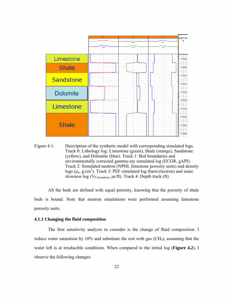
The synthetic case (Figure 4.1) consists of six beds: the top five beds consist of

approximately equal-thickness layers of pure limestone, shale, sandstone, dolomite, and

an additional layer of limestone. All these beds are initially saturated with water. The

bottom layer consists of a thicker shale bed.

DolomiteDolomite

Figure 4.1: Description of the synthetic model with corresponding simulated logs. Track 0: Lithology log: Limestone (green), Shale (orange), Sandstone (yellow), and Dolomite (blue). Track 1: Bed boundaries and environmentally corrected gamma-ray simulated log (ECGR, gAPI). Track 2: Simulated neutron (NPHI, limestone porosity units) and density logs (ρα, g/cm3). Track 3: PEF simulated log (barn/electron) and sonic slowness log (VP,formation, μs/ft). Track 4: Depth track (ft).

All the beds are defined with equal porosity, knowing that the porosity of shale

beds is bound. Note that neutron simulations were performed assuming limestone

porosity units.

4.1.1 Changing the fluid composition

The first sensitivity analysis to consider is the change of fluid composition: I

reduce water saturation by 10% and substitute the rest with gas (CH4), assuming that the

water left is at irreducible conditions. When compared to the initial log (Figure 4.2), I

observe the following changes:

22

The density decreases by an average of 0.65 g/cm3 while remaining constant

within shale beds.

The neutron simulation decreases by an average of 21% while remaining

constant within shale beds.

The sonic model decreases by an average of 82 μs/ft while remaining constant

within shale beds.

The GR simulation remains unaffected.

Figure 4.2: Simulated logs for the synthetic model with 90% of methane in fluid saturations. Track 0: Lithology log: Limestone (green), Shale (orange), Sandstone (yellow), and Dolomite (blue). Track 1: Bed boundaries and environmentally corrected gamma-ray simulated log (ECGR, gAPI). Track 2: Simulated neutron (NPHI, limestone porosity units) and density logs (ρα, g/cm3). Track 3: PEF simulated log (barn/electron) and sonic slowness log (VP,formation, μs/ft). Track 4: Depth track (ft).

23

4.1.2 Including an additional layer

This time, I introduce a layer of anhydrite with low radioactivity content above

the bottom layer. As expected, the GR simulation across that layer is negligible (almost 0

gAPI), whereas the neutron and density simulations yielded relatively considerable

changes (Figure 4.3). In fact, the neutron density was set to 12% (limestone porosity

units) while the recorded density was 2.8 g/cm3.

Figure 4.3: Simulated logs for the synthetic model with an additional layer of anhydrite. Track 0: Lithology log: Limestone (green), Shale (orange), Sandstone (yellow), Dolomite (blue), and Anhydrite (red). Track 1: Bed boundaries and environmentally corrected gamma-ray simulated log (ECGR, gAPI). Track 2: Simulated neutron (NPHI, limestone porosity units) and density logs (ρα, g/cm3). Track 3: PEF simulated log (barn/electron) and sonic slowness log (VP,formation, μs/ft). Track 4: Depth track (ft).

24

4.1.3 Modifying porosity

In this case, I increase the total porosity of all the beds from 20% to 35%. The

updated results (Figure 4.4) indicate an increase of 33 μs/ft in the sonic log and 0.21

g/cm3 in the density, while GR and PEF are barely altered. While all the sonic and the

density logs experience a constant increase, the neutron simulation exhibits a decrease of

12.8% (limestone porosity units) instead. Note that all these changes are observed in

non-shale beds.

Figure 4.4: Simulated logs for the synthetic model after modifying the overall porosity. Track 0: Lithology log: Limestone (green), Shale (orange), Sandstone (yellow), and Dolomite (blue). Track 1: Bed boundaries and environmentally corrected gamma-ray simulated log (ECGR, gAPI). Track 2: Simulated neutron (NPHI, limestone porosity units) and density logs (ρα, g/cm3). Track 3: PEF simulated log (barn/electron) and sonic slowness log (VP,formation, μs/ft). Track 4: Depth track (ft).

25

4.1.4 Including an additional mineral in the bulk solid composition

Unlike previous modifications that dealt with pure minerals in each bed, I set the

volumetric concentration of quartz equal to 30% in each layer (Figure 4.5). This time,

sonic and density logs are readjusted mainly at shale beds, while the remaining layers are

marginally affected. The sonic log exhibits an increase of 30 μs/ft while the density log

decreases by 0.39 g/cm3.

Figure 4.5: Simulated log of the synthetic model with a modified matrix composition. Track 0: Lithology log: Limestone (green), Shale (orange), Sandstone (yellow), and Dolomite (blue). Track 1: Bed boundaries and environmentally corrected gamma-ray simulated log (ECGR, gAPI). Track 2: Simulated neutron (NPHI, limestone porosity units) and density logs (ρα, g/cm3). Track 3: PEF simulated log (barn/electron) and sonic slowness log (VP,formation, μs/ft). Track 4: Depth track (ft).

26

4.1.5 Adding thinly-bedded layers

In this final simulation experiment, I include a sequence of adjacent thin beds of

sand and shale. The outcome of the simulation (Figure 4.6) emphasizes the importance

of the choice of simulation sampling rate, since it is not capable of resolving the thinly-

bedded layers, specifically in depths ranging from 17932 ft to 17924 ft. It is imperative to

choose a sampling rate smaller than the thinnest bed in the defined model in order to

obtain a reliable result.

Figure 4.6: Simulated logs for the synthetic model with a sequence of thin beds of sand and shale. Track 0: Lithology log: Limestone (green), Shale (orange), Sandstone (yellow), Dolomite (blue), and a sequence of thin beds of shale and sand (brown). Track 1: Bed boundaries and environmentally corrected gamma-ray simulated log (ECGR, gAPI). Track 2: Simulated neutron (NPHI, limestone porosity units) and density logs (ρα, g/cm3). Track 3: PEF simulated log (barn/electron) and sonic slowness log (VP,formation, μs/ft). Track 4: Depth track (ft).

27

28

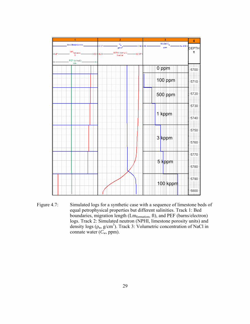
4.1.6 Salinity effect on nuclear logs

Concerning this example, a different synthetic model was used:

I construct 8 water-filled adjacent beds of thicknesses ranging from 8 to 13 ft.

I set the same petrophysical properties for each layer but vary the volumetric

concentration of NaCl in their connate water from 0 to 100 kppm.

I choose pure limestone for the matrix composition and assume a negligible

change of temperature.

Figure 4.7 describes the effect of changing the salinity of connate water on nuclear logs,

notably PEF, Density, and Neutron.

I observe that the higher the salinity, the lower the values of density, neutron, and

PEF. I also observe that the change is more noticeable whenever Cw exceeds 5 kppm.

This is an important observation to consider whenever there is an offset between

simulated and field logs, which would indicate the need of an adjustment of the water

salinity of the layers.

0 ppm

100 ppm

500 ppm

1 kppm

3 kppm

5 kppm

100 kppm

0 ppm

100 ppm

500 ppm

1 kppm

3 kppm

5 kppm

100 kppm

0 ppm

100 ppm

500 ppm

1 kppm

3 kppm

5 kppm

100 kppm

Figure 4.7: Simulated logs for a synthetic case with a sequence of limestone beds of equal petrophysical properties but different salinities. Track 1: Bed boundaries, migration length (Lmformation, ft), and PEF (barns/electron) logs. Track 2: Simulated neutron (NPHI, limestone porosity units) and density logs (ρα, g/cm3). Track 3: Volumetric concentration of NaCl in connate water (Cw, ppm).

29

30

4.2 FIELD STUDIES

In this section, I test the full procedure on field examples. The cases contain

descriptive situations encountered in practice, such as carbonate, siliciclastic, thinly-

bedded, and offshore formations. Based on the type of data available, different methods

are considered in order to establish the final assessments, emphasizing the manual

iterative procedure, initial guess, and full log analysis.

4.2.1 Carbonate Formation

The field logs to be interpreted correspond to a carbonate sequence (Figure 4.8a

& 4.8b, shown in blue). This sequence describes a carbonate reservoir that contains a

high amount of secondary porosity. The carbonate sediments mainly consist of thinly- to

thickly-bedded dolomite with complex depositional and diagenetic features (Miranda,

2008). Beds were initially deposited from grain-rich up to mud-rich carbonates.

Subsequently, they underwent diagenesis that significantly modified their fabric, texture,

and petrophysical properties.

I first define bed boundaries where I identify a considerable change in the

composition based on GR variations. The minimum variation considered for detecting a

bed boundary is 75%, and the number of beds is approximately 13. Then, for each bed

separately, the palette is used to input the composition based on log analysis. After all

layers definitions are entered, nuclear-log simulations are executed. Gamma-ray, density,

and neutron logs are plotted to be compared to their corresponding field logs. If the

simulations (Figures 4.8a and 4.8b, shown in red) at certain depth intervals do not agree

with field logs then an iterative refinement step is added, which consists of redefining bed

properties by either partitioning them into smaller beds or by redefining the compositions

and volumetric concentrations of the bed.

LegendSee legend

Lithology-0---------fraction----------1-

LegendLegendSee legend


See legend


Figure 4.8a: Field and simulated logs for the carbonate example. Track 1: Depth track (ft). Track 2: Bed boundaries and caliper (ft). Track 3: Lithology (fraction): orthoclase (grey), quartz (yellow), biotite (green), dolomite (purple), limestone (black), glauconite (orange), illite (gold), water (blue), shale water (light blue), oil (red). Track 4: GR (gAPI). Track 5: Density (g/cm3). Track 6: Neutron (limestone porosity units). Track 8: PEF (barn/electron).

31

LegendSee legend

Lithology-0-------fraction--------1-



See legend


Figure 4.8b: Field and simulated logs for the carbonate example. Track 1: Depth track (ft). Track 2: Bed boundaries and caliper (ft). Track 3: Lithology (fraction): orthoclase (grey), quartz (yellow), biotite (green), dolomite (purple), limestone (black), glauconite (orange), illite (gold), water (blue), shale water (light blue), oil (red). Tracks 4 to 8: High-Resolution Laterolog Array Tool from shallow to deeper radial lengths of investigation (Ω.m).

32

LegendSee legend

Lithology-0-----------------fraction-----------------1-



See legend


Figure 4.8c: Spatial distribution of resistivity and water saturation. Track 1: Depth track (ft). Track 2: Lithology (fraction): orthoclase (grey), quartz (yellow), biotite (green), dolomite (purple), limestone (black), glauconite (orange), illite (gold), water (blue), shale water (light blue), oil (red). Track 3: GR (gAPI). Track 4: High-Resolution Laterolog Array Tool (Ω.m). Track 5: Water saturation (fraction).

33

34

Results show that the percentage of clay in layers that exhibit high gamma-ray is

relatively high; quantitatively, in the top layer, I observe 41% illite and 18% glauconite,

while the bottom layer exhibits 52% of illite and 24% glauconite content. Layers that

have the lowest gamma-ray values mainly consist of dolomite (71% dolomite for the

depth interval 11712 to 11728 ft). I also observed that the highest values of neutron

porosity were located in the top (32% limestone porosity units) and bottom (28%

limestone porosity units) layers. The reason behind this effect is the high hydroxyl

content in the clay included in those layers. The average relative error in the PEF log is

3%, which implies a reliable match.

Concerning the simulated resistivity logs (Figure 4.8b), I observe a constant

under-estimation of the resistivity values in the upper quarter of the formation, and a

constant over-estimation in the interval that lies between 11728 ft and 11750 ft. The

most probable reason behind these offsets is due to the fact that resistivity logs were the

last to be matched. The colored spatial distribution of the simulated resistivity and water

saturation results (Figure 4.8c) indicates that the drilling mud was water-base, since the

radial distribution interval from 11692 ft to 11699 ft shows a lower resistivity from the

borehole wall to the radial distance of 1 ft. Finally, I observe a deep WBM-filtrate

invasion in the interval from 11728 ft to 11750 ft.

4.2.2 Siliciclastic Formation

The purpose of this example is to apply a similar matching procedure to a

siliciclastic formation. The field logs to be interpreted were acquired in a mixed rock

sequence, predominantly siliciclastic, as included in the calculated lithology log. Based

on the core description, the sequence is a sandy limestone, half of which includes calcite

with a trace of dolomite. Moreover, the limestone is interspersed as thin siltstone beds.

Figure 4.9a is a previous lithology work that I use as initial guess.

A procedure similar to that of the previous example is used for detecting bed

boundaries, since both sequences belong to the same wellbore but are situated at different

depths. Water saturation (Sw) was computed through Archie’s equation (1942) i.e., n

t

wmw R

RaS

/1

. (4.1)

Where a is tortuosity factor, Rw is connate water resistivity, is effective porosity, and m

and n are cementation and saturation exponents, respectively. For this field case, I

assumed values of 1.84 and 2 for the cementation and saturation exponents respectively,

while the tortuosity factor is taken as 1.

As in the previous example, I did not attempt to match all the small log variations

but rather concentrated on matching the general trends for each layer. Figure 4.9b

describes the match between the field logs (in blue) and simulated models (in red). Note

that the abrupt change around the depth of 11,146 ft signaled in the caliper log caused an

error in the GR log; therefore, I did not include it in the matching procedure.

In layers with substantial amounts of limestone (80% volumetric fraction), the

density log measures an increase of 0.3 g/cm3, while the neutron log measures a decrease

of 12% (sandstone porosity units). Moreover, the simulated PEF exhibits a larger increase

in the layers with higher volumetric fraction of limestone (from 11070 ft to 11075 ft,

from 11105 ft to 11117 ft, and from 11123 ft to 11145 ft). The opposite trend takes place

for the case of the sonic log.

From this formation, I conclude that the high concentration of limestone in a

siliciclastic sequence results in high measured values of density and PEF logs, and low

35

measured values of neutron and sonic logs. Hence, the iterative procedure makes it easier

to detect such a combination of minerals.

10

9

876

5

4

3

2

1

10

9

876

5

4

3

2

1

10

9

876

5

4

3

2

1

Figure 4.9a: Lithology log used as the starting point for the assessment of lithology and petrophysical properties of layers. Left column represents the user-defined layers. Track 1: Bulk mineral composition. Track 2: Fluid composition.

36

Legend

See legend

Lithology-0----fraction---1-

LegendLegend

See legend

Lithology-0----fraction---1-

Figure 4.9b: Field and simulated logs for the siliciclastic example. Track 1: Depth track (ft). Track 2: Bed boundaries and caliper (ft). Track 3: Lithology (fraction): quartz (yellow), limestone (red), illite (grey), water (blue), shale water (light blue). Track 4: GR (gAPI). Track 5: Density (g/cm3). Track 6: Neutron (sandstone porosity units). Track 7: PEF (barn/electron). Track 8: Sonic slowness (μs/ft). Track 9: High-Resolution Laterolog Array Tool of deepest radial length of investigation (Ω.m).

37

38

4.2.3 Case w

The purpose of this field exam

observed field logs by using sp

cases, the study of this sequence w

core data. Hence, full log analysis had to

properties. The availab

litho

determ

of sm

ith available spectral GR logs

ple is to enhance the agreement between simulated and

ectral GR logs in the initial approach. Unlike previous

as entirely based on logs and a minimal amount of

be performed to calculate petrophysical

ility of the spectral GR logs was beneficial to initialize the

logical composition. The thorium vs. potassium cross-plot (Figure 4.10) helped to

ine the types of clay existing in the formation. In this case, I inferred the presence

ectite, kaolinite and some chlorite along different beds.

0

5

10

15

20

25

0 0.5 1 1.5

Th

ori

um

(p

pm

)

2 2.5 3 3.5 4 4.5 5

Potassium (%)

1 2 3 4 5 6 7 8 9 10 11 12 13 14 15 16

Bed number:

Figure 4.10:

Left: Track 1: Depth track (ft). Track 2: GR log (gAPI) and petrophysical bed boundaries. Right: thorium vs. potassium cross-plot for field example 3 used to infer types of clay contained in the sequence. Beds are numbered from top to bottom.

39

The log shown in Figures 4.11a and 4.11b show the initial model defined based on

results imported from the log analysis into the palette. Moreover, the previous cross-plot

was combined with the GR log, which allowed me to differentiate between shale and

sand beds, as well as to define the types of clay existing in each individual bed.

I first observe 8 major shale beds, in which the amount of bound water is high

(12% volumetric concentration), while hydrocarbon is contained between these layers. I

also observe a clear shale baseline in the simulated resistivity log, which is

Schlumberger’s Micro-Spherically Focused Conductivity Tool. As emphasized earlier in

field case No. 1, the neutron log exhibits a large increase (27% sandstone porosity units)

whenever the clay content is considerable (70% clay concentration). In addition, low

porosity in clays resulted in high sonic slowness values (an average increment of 18

μs/ft).

Once the model was built, minor adjustments were needed on the spectral GR of

minerals and clays, since these values can vary based on different geographic locations.

Thorium, potassium and uranium values can be improved using the log values at pure

shale sequences.

Based on this example, I conclude that the availability of spectral GR logs greatly

helps to assess clay mineralogy, and hence in achieving an improved match between

simulated and field logs.

See legend

Legend

Lithology-0-------------fraction---------------1-

See legendSee legend

LegendLegend

Lithology-0-------------fraction---------------1-

Figure 4.11a: Field and simulated logs for example No. 3. Track 1: Depth track (ft). Track 2: Bed boundaries and caliper (ft). Track 3: Lithology (fraction): quartz (yellow), smectite (grey), kaolinite (brown), illite (purple), shale water (dark blue), water (blue), hydrocarbon (red). Track 4: GR (gAPI). Track 5: thorium concentration (ppm). Track 6: uranium concentration (ppm). Track 7: potassium concentration (%). Track 8: Apparent Spherically Focused Resistivity (Ω.m).

40

Legend

See legend

Lithology-0-------------fraction-----------1-

LegendLegend

See legendSee legend

Lithology-0-------------fraction-----------1-

Figure 4.11b: Field and simulated logs for example No. 3. Track 1: Depth track (ft). Track 2: Bed boundaries and caliper (ft). Track 3: Lithology (fraction): quartz (yellow), smectite (grey), kaolinite (brown), illite (purple), shale water (dark blue), water (blue), hydrocarbon (red). Track 4: GR (gAPI). Track 9: Density (g/cm3). Track 10: Neutron (sandstone porosity units). Track 11: Sonic slowness (μs/ft).

41

42

4.2.4 Case with an illustrated manually-iterated procedure

The sequence analyzed in this case is a North Louisiana’s tight-gas sand (Heidari

et al., 2009). Despite the lack of core data, we know that this sequence was drilled with

water-based mud (WBM). Resistivity logs show a significant separation, which indicates

deeply invaded beds; nonetheless, I observe a substantial cross-over between neutron and

density logs. This cross-over indicates the existence of residual gas saturation and

irreducible water. With the amount of information I have, I am forced to start with a

vague estimate of petrophysical properties and subdivide the sequence into a small

number of beds. This allows me to quickly obtain an initial model, from which I can

focus on each bed separately by splitting them into smaller ones that will be adjusted and

redefined afterward. Such method is often referred to as the ‘divide and conquer’

approach, a known technique to minimize the number of steps needed to obtain the final

solution when sparse information is available. Concerning this case, I started with only

four beds based on the variations observed in both density and compensated neutron logs.

At first, I assumed that I was dealing with a siliciclastic sequence, but density and

neutron results were shifted by an average of 22%. Assuming a carbonate formation

provided a much closer fit (error reduced to 4%), which I confirmed afterward when I

received more information about the sequence (Figure 4.12a).

Field example No. 4: First iteration based on the carbonate assumption. Track1: Depth track (ft). Track 2: Caliper (ft) and bed boundaries. Track 3: Field and simulated GR logs (gAPI). Track 5: Neutron (limestone porosity units) and Density (g/cm3) field logs, water (green) and hydrocarbon cross-over (yellow). Track 6: Neutron (limestone porosity units) and Density (g/cm3) simulated logs, water (green) and hydrocarbon cross-over (yellow).

43

Figure 4.12a:

44

At the second iteration, I subdivided the thicker layers to obtain a total of 12

define new layers from the beginning since I already had a

atch initially. The second iteration was more time consuming, but it would have

ore cumbersome if I skipped the first one (Figure 4.12b).

layers. I did not have to re

close m

been m

readjus

been fine-tuned along with the rem

provided the ability to obtain

m

this stage, which resulted in exhibiting a good

both density and neutron logs

water. Furtherm

presence of residual gas saturation. Moreover, th

f

this can be an error due to borehole enla

realized th

sim

Once the model appears consistent enough, I consider the resistivity log and start

ting porosities and water saturations. This is also a tedious process that could have

aining logs at the iteration level, but would have

a quick glimpse at the intermediary results longer.

Figure 4.13 shows the final outcome of this work after two iterations, and gives

e a good assessment of the sequence. Resistivity simulations were performed only at

match (3% error) to field logs. Note that

had to be adjusted by increasing the salinity of connate

ore, the large cross-over between density and neutron logs indicated the

e peak in the GR log at the depth of 2675

t was not observed in the simulated logs since it correlated with in the caliper log; hence,

rgement. Throughout this field example, I

at doing a series of iterative modeling yielded a better agreement between

ulated and field logs.

Second iteration applied on the previous model. Track1: Depth track (ft). Track 2: Caliper (ft) and bed boundaries. Track 3: Field and simulated GR logs (gAPI). Track 4: Neutron (sandstone porosity units) and Density (g/cm3) field logs, water (green) and hydrocarbon cross-over (yellow). Track 5: Neutron (limestone porosity units) and Density (g/cm3) simulated logs, water (green) and hydrocarbon cross-over (yellow). Track 6: Sonic slowness (μs/ft).

45

Figure 4.12b:

Figure 4.13: Final model after the introduction of the resistivity log. Track1: Depth track (ft). Track 2: Caliper (ft), bed boundaries, and petrophysical bed boundaries. Track 3: Field and simulated GR logs (gAPI). Track 4: Field and simulated Neutron (sandstone porosity units) logs. Track 6: Field and simulated Density (g/cm3) logs. Track 7: Sonic slowness (μs/ft). Track 8: Neutron (sandstone porosity units) and Density (g/cm3) field logs, water (green) and hydrocarbon cross-over (yellow). Track 9: Neutron (limestone porosity units) and Density (g/cm3) simulated logs, water (green) and hydrocarbon cross-over (yellow).

46

47

4.2.5 Offshore Formation

The example has been previously considered by Angeles et al. (2009). This

sequence describes a siliciclastic offshore reservoir, dated between upper Paleocene and

lower Eocene. The well is situated under approximately 6500 ft of water.

When combining a high GR response with a clear separation between density and

neutron logs (Figure 4.14a), I infer the existence of high volumes of shale in the

formation. Hence, I used the dual-water model (Clavier et al., 1984) to calculate water

saturation (free and clay-bound). The parameters I used for the model are a=1, m=1.9,

and n=2.1.

Figure 4.14b shows the resulting simulated resistivity curves after simulating

invasion with the Invasion Module. Note that the relatively large separation between the

resistivity curves at the bottom half of the formation confirms the presence of mobile

water. Therefore, the match had to be modified by adjusting the amount of irreducible

water saturation. On the other hand, I chose to have a finer grid for the simulation of the

top half of the sequence, which led to an average error of 3.5%.

Unlike the previous examples, I tried to match the resistivity logs prior to

matching density and neutron logs; this resulted in a fairly larger error in the simulated

density log (roughly 6.9%), while the simulated neutron log agreed with its

corresponding field log (average error of 2.55%) (Figure 4.14a). Even though the

simulated density log did not agree well with the field log, the error was not significant.

Hence, changing the order of logs to be matched leads to approximately the same result.

Finally, the simulated GR log matched the corresponding field log with an average error

of 3.2%.

Legend

See legend

Lithology-0--------------fraction---------------1- Legend

See legend

Lithology-0--------------fraction---------------1-

Field and simulated logs for the offshore formation. Track 1: Bed boundaries, petrophysical bed boundaries and caliper (ft). Track 2: Lithology (fraction): quartz (yellow), biotite (brown), orthoclase (green), illite (grey), chlorite (pink), glauconite (dark green), shale water (dark blue), water (blue), oil (red). Track 3: GR (gAPI). Track 4: Density (g/cm3). Track 5: Neutron (sandstone porosity units). Track 6: Depth track (ft).

48

Figure 4.14a:

LegendSee legend

Lithology-0-------------fraction--------------1-


Lithology-0-------------fraction--------------1-

Figure 4.14b: Field and simulated logs for the offshore formation. Track 1: Bed boundaries, petrophysical bed boundaries and caliper (ft). Track 2: Lithology (fraction): quartz (yellow), biotite (brown), orthoclase (green), illite (grey), chlorite (pink), glauconite (dark green), shale water (dark blue), water (blue), oil (red). Tracks 6 to 10: Array Induction Two Foot Resistivity Tool from shallow to deeper depths of investigation (Ω.m).

49

50

CHAPTER 5

SUMMARY AND CONCLUSIONS

5.1 SUMMARY

I described a new method for interactive modeling and simulation of nuclear logs.

Simulations were performed with a linear iterative refinement technique introduced by

Mendoza (2009). The subsurface model under consideration consisted of horizontal beds

with variable chemical compositions and volumetric concentrations of solid and fluid

constituents. The use of core information, performing a full log analysis, and/or refining

an initial guess by manually iterating a model is crucial to obtaining reliable simulations.

Users enter constituents and their compositions via a choice palette. Subsequently,

Schlumberger’s SNUPAR software is used to calculate nuclear properties necessary for

the simulation of nuclear logs.

5.2 CONCLUSIONS

Testing of the software with synthetic, as well as field cases confirmed its

applicability for the interactive matching of field logs. Despite difficulties and limitations

associated with either unavailable data or uncertainty of some parameters, simulation

methods used with the interactive procedure proved to be reliable.

51

In some situations, the trend of simulations obtained with the module was

accurate but not the values. If such condition takes place for the case of gamma-ray or

sonic logs, an adjustment is necessary in the spectral mineral values or sonic slowness .

The six synthetic cases indicated changes in nuclear simulations when making

one modification at a time of the petrophysical properties of homogeneous beds. These

modifications consisted of changing fluid/mineral composition, water salinity, porosity,

adding an additional layer, or including thinly-bedded layers.

The five field examples described in this thesis revealed key factors about the

approach to use when initializing a model:

- In the first example, I learned that the last log to be matched will have the highest

error margin (ranging from 1.4% to 13.3%). Therefore, it is best to choose carefully

the order of logs to be matched depending on their confidence level.

- In the second example, when dealing with a mixed siliciclastic-carbonate sequence

primarily, the amount of limestone could be readily discerned from density, PEF, and

neutron logs.

- In the third example, the availability of spectral GR logs greatly improved the

petrophysical assessment of a formation; indeed, the thorium vs. potassium cross-plot

was an efficient starting point to determine clay content.

- In the fourth example, I observed that when important information is missing about a

formation, the ‘divide and conquer’ approach is the best option to perform the

modeling process. It minimizes the numbers of steps needed to obtain the final

solution. Moreover, using the iterative modeling technique results in a better match

between simulated and field logs.

- In the last example, I used two approaches to solve the problem. The first one was to

match the resistivity logs prior to matching neutron and density logs and the second

52

approach was to match the neutron and density logs before proceeding with the

resistivity match. I observed that the error factor in the first approach was reduced by

a factor of half compared to that of the second approach. Therefore, the order of

matching logs is critical.

Furthermore, the options provided throughout the interactive modeling can

narrow down the number of variables needed to initialize the simulations by testing one

option at a time when current simulated results do not match field logs.

Even though simulated results are in close agreement with field logs, there were

cases where the match in the PEF log was not as satisfactory as with other logs.

In this thesis, I introduced and successfully tested the concept of interactive

modeling and interpretation of nuclear logs. I showed that numerical simulation and

matching of field logs using fast modeling procedures is a practical method to improve

the assessment of inferred static and dynamic formation petrophysical properties.

53

Appendix A

Detailed Inventory of Well Logs Available for the Field Cases

Table A.1 is a detailed inventory of well logs available for the case studies. It also

identifies those wells with rock-core measurements. The terminology used to designate

each well log in this table is explained in the nomenclature section. The last column of

this table describes the availability of core analysis information.

Case

#

SP Caliper GR Spectral

GR

RHOB NPHI PEF Resis DT Core

1

2

3

4

5

Table A.1: Detailed inventory of well logs available for this study.

Appendix B

Archie’s Equation and Summary of Parameters Considered for the Modeling of Water Saturation Curves

This appendix describes the parameters included in Archie’s equation. It also

summarizes the parameters used for calculating water saturation.

In order to obtain Sw, Sxo and Sh, we apply Archie’s equation, given by n

t

wmw R

RaS

/1

, (B.1)

where a is tortuosity factor, Rw is connate water resistivity, is porosity, and m and n are

cementation and saturation exponents, respectively. In the carbonate and siliciclastic

cases, the tortuosity factor is taken as 1 in equation 3.8 based on the type of lithology

already observed in the description. Connate-water resistivity at reservoir conditions was

estimated using a salinity of 6700 ppm, whereupon Rw is equal to 0.23 Ω.m at reservoir

temperature.

54

Appendix C

Dual-Water Equation and Summary of Parameters Considered for the Modeling of Water Saturation Curves

This appendix describes the usage of the dual-water method for shaly sands

(Clavier et al., 1984). In order to obtain Sw, I read Rt, and GR in the sand of interest, in

a nearby shale, and in a clean sand. After calculating Csh, correcting the porosities for

shaliness, and calculating the non-shale porosity, I determine the total porosity of the

nearby shale using shN

shD

sht )1( , (C.1)

where 0.5≤ ≤0.9. The bound-water fraction of the sand is then given by sht

b sht

S C

, (C.2)

with sh

t e sh tC , (C.3)

and msh

tb shR R

a

, (C.4)

with a = 1, m = 1.9, and n = 2.1 for the field example No. 5. It follows that

b

w

w

bmt

nw

w

mtn

wt R

R

Ra

SS

RaS

R1

1 , (C.5)

where Sw is the dual-water saturation.

55

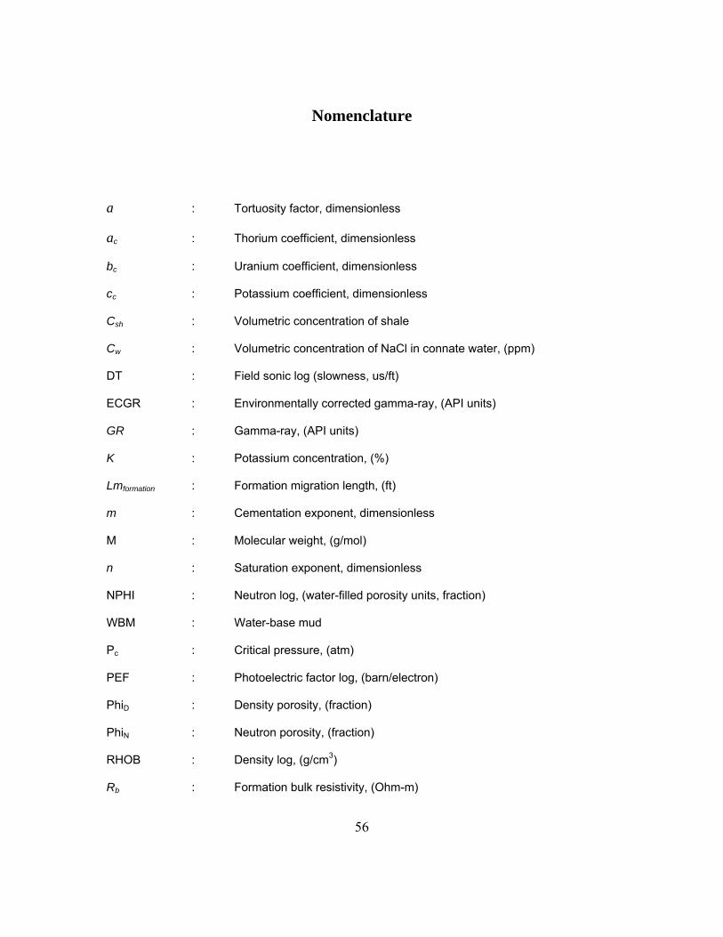
56

Nomenclature

a : Tortuosity factor, dimensionless

ac : Thorium coefficient, dimensionless

bc : Uranium coefficient, dimensionless

cc : Potassium coefficient, dimensionless

Csh : Volumetric concentration of shale

Cw : Volumetric concentration of NaCl in connate water, (ppm)

DT : Field sonic log (slowness, us/ft)

ECGR : Environmentally corrected gamma-ray, (API units)

GR : Gamma-ray, (API units)

K : Potassium concentration, (%)

Lmformation : Formation migration length, (ft)

m : Cementation exponent, dimensionless

M : Molecular weight, (g/mol)

n : Saturation exponent, dimensionless

NPHI : Neutron log, (water-filled porosity units, fraction)

WBM : Water-base mud

Pc : Critical pressure, (atm)

PEF : Photoelectric factor log, (barn/electron)

PhiD : Density porosity, (fraction)

PhiN : Neutron porosity, (fraction)

RHOB : Density log, (g/cm3)

Rb : Formation bulk resistivity, (Ohm-m)

57

Rcl : Clay formation resistivity, (Ohm-m)

Rt : True formation resistivity, (Ohm-m)

Rw : Connate water resistivity, (Ohm-m)

Rw,a : Apparent water resistivity in shaly sand, (Ohm-m)

Rxo : Flushed-zone formation resistivity, (Ohm-m)

SP : Spontaneous potential, (mV)

Sb : Bound-water fraction of sand, (fraction)

Sw : Water saturation, (fraction)

Sw,t : Total water saturation corrected for shale, (fraction)

Tc : Critical temperature, (K)

Th : Thorium concentration, (ppm)

U : Uranium concentration, (ppm)

VP,formation : Sonic slowness model, (μs/ft)

Greek symbols

Θ : Contact angle between the fluid interface and the rock, (degrees)

ω : Acentric factor, dimensionless

Δt : Sonic slowness, (μs/ft)

Δtb : Sonic slowness of pure bulk, (μs/ft)

Δtf : Sonic slowness of pure fluid, (μs/ft)

Δts : Sonic slowness of pure solid, (μs/ft)

Δtsh,f : Sonic slowness of the shale fluid, (μs/ft)

Δtsh,s : Sonic slowness of the shale solid, (μs/ft)

ρα : Simulated density, (g/cm³)

ρf : Fluid density, (g/cm³)

ρma : Matrix density, (g/cm³)

: Porosity, (fraction)

DC : Porosity obtained from bulk density log corrected for presence of shale, (fraction)

b : Bulk density log in a pure shale, (fraction)

e : Non-shale porosity, (fraction)

cl : Clay porosity, (fraction)

NS : Non-shale porosity, (fraction)

NC : Porosity calculated from neutron log corrected for presence of shale, (fraction)

N : Porosity calculated from neutron log without corrections for presence of shale,

(fraction)

Nsh : Neutron log response in a pure shale, (fraction)

sht : Total porosity of shale, (fraction)

shD : Density porosity of shale, (fraction)

shN : Neutron porosity of shale, (fraction)

58

59

References

Angeles, R., Torres-Verdín, C., Sepehrnoori, K., and Elshahawi, H., "History Matching

of Multiphase-Flow Formation-Tester Measurements Acquired with Focused-Sampling Probes in Deviated Wells." In SPWLA 50th Annual Logging Symposium, 4-7. Houston, TX, 2009.

Aristodemou, E., C. Pain, C. de Oliveira, A. Umpleby, T. Goddard, and C. Harris.

"Energy Group Optimization for Forward and Inverse Problems in Nuclear Engineering: Application to Downwell-Logging Problems." Geophysical Prospecting 54 (2006): 99-120.

Clavier, C., Schlumberger Technical Services, G. Coates, J. Dumanoir, and Schlumberger

Well Services. "The Theoretical and Experimental Bases for The "Dual Water" Model for the Interpretation of Shaly Sands." SPE Journal 21, (1984): 153-68.

Ellis, D. V., Case, C. R., and Chiaramonte, J. M., "Porosity from Neutron Logs I:

Measurement." Petrophysics 44, no. 6, (2003): 383–95. ———. "Porosity from Neutron Logs II: Interpretation." Petrophysics, 45, no. 1 (2004):

73-86. Heidari, Z., Torres-Verdín, C., Mendoza, A., and Wang, G. L., "Improving the

Assessment of Residual Hydrocarbon Saturation with the Combined Quantitative Interpretation of Resistivity and Nuclear Logs." In SPWLA 50th Annual Logging Symposium, 8-10. Houston, TX, 2009.

"Log Interpretation Charts." Schlumberger Information Solutions,

http://www.slb.com/content/services/resources/books/log_charts/index.asp. McKeon, D. C., and Scott, H. D., "Snupar-a Nuclear Parameter Code for Nuclear

Geophysics Applications." IEEE Transactions on Nuclear Science 36, no. 1 (1989): 1215-19.

Mendoza, A., Preeg, W. E., Torres-Verdín, C., and Alpak, F. O., "Monte Carlo Modeling

of Nuclear Measurements in Vertical and Horizontal Wells in the Presence of Mud-Filtrate Invasion and Salt Mixing." Petrophysics, 48, no. 1 (2007): 28-44.

http://www.slb.com/content/services/resources/books/log_charts/index.asp

60

Mendoza, A., Torres-Verdín, C., and Preeg, W. E., "Rapid Simulation of Borehole Nuclear Measurements with Approximate Spatial Flux-Scattering Functions." In SPWLA 48th Annual Symposium, 6-10. Austin, TX, 2007.

Mendoza, A. "Rapid Numerical Simulation and Inversion of Nuclear Borehole

Measurements Acquired in Vertical and Deviated Wells." 5-16: Ph.D. Dissertation, The University of Texas at Austin, 2009.

"Mineral Mnemonics." Schlumberger Information Solutions,

http://www.slb.com/modules/mnemonics/Mineral.aspx. Miranda, L. J., "Mud-Filtrate Invasion Modeling to Quantify Static and Dynamic

Petrophysical Properties of Fractured and Vuggy Carbonate Formations." Master’s Thesis, The University of Texas at Austin, 2008.

Peng, Ding-Yu, and Robinson, D. B. "A New Two-Constant Equation of State."

Industrial and Engineering Chemistry: Fundamentals, 15 (1976): 59-64. Radtke, R. J., Evans, M., Rasmus, J. C., Ellis, D. V., Chiaramonte, M., Case, C. R., and

Stockhausen, E., "LWD Density Response to Bed Laminations in Horizontal and Vertical Wells." Petrophysics, 48 (2007): 76.

Sherman, H., and Locke, S., "Effect of Porosity on Depth of Investigation of Neutron and

Density Sondes." Paper presented at the Fall Meeting of the Society of Petroleum Engineers of AIME, 1975.

Tittle, C. W. "Diffusion Theory Models of Invasion for Nuclear Porosity Tools." Paper

presented at the 33rd Annual Logging Symposium Transactions: SPWLA, 1992. The University of Texas at Austin Petrophysical and Well-Log Simulator (UTAPWeLS)

©, User Guide. Austin, TX: Formation Evaluation Group, The University of Texas at Austin, 2009.

Watson, C. C. "Monte Carlo Computation of Differential Sensitivity Functions." Trans.

Am. Nucl. Soc. 46 (1984): 665. Wiley, R., and Patchett, J. G., "The Effects of Invasion on Density/Thermal Neutron

Porosity Interpretation." Paper presented at the 35th Annual Logging Symposium Transactions: SPWLA, 1994.

Wyllie, M. R. J., Gregory, A. R., and Gardner, L. W., "Elastic Wave Velocities in

Heterogeneous and Porous Media." Geophysics, 21 (1956).

http://www.slb.com/modules/mnemonics/Mineral.aspx

61

X-5_Monte_Carlo_Team_MCNP. A General Monte Carlo N-Particle Transport Code. 5 ed. Vol. III. Los Alamos, New Mexico: developer's guide: University of California, Los Alamos National Laboratory, 2003.

62

Vita

Malek Mohamed Lemkecher was born in Tunis, Tunisia on September 17, 1983,

the third and youngest son of Bakhta Ben Zaied and Boubaker Lemkecher. After

graduating from the nationally elite Pioneer School of Ariana, in 2002, he moved to the

United States of America to earn a Bachelor’s degree of Science in Computer

Engineering at Texas A&M University. In 2007 he entered the Graduate School of The

University of Texas at Austin to pursue a Master’s of Science degree in Petroleum

Engineering. He has a strong belief that mixing the electrical, computer, and petrophysics

disciplines will lead to a great improvement in the speed and accuracy of petroleum

engineering solutions.

Permanent address: 8, rue 7214 El Menzah 9A

1013 Tunis

TUNISIA

This thesis was typed by the author.

Copyright by Malek Mohamed Lemkecher 2009

Documents

Transcript of Copyright by Malek Mohamed Lemkecher 2009