i

Copyright

by

Gilberto Lopez

2002

ii

Classification and Testing of Paved Road Surfaces for

Vehicle and Tire Modeling

by

Gilberto Lopez, B.S.

Thesis

Presented to the Faculty of the Graduate School

of The University of Texas at Austin

in Partial Fulfillment

of the Requirements

for the Degree of

Master of Science in Engineering

The University of Texas at Austin

December 2002

iii

Classification and Testing of Paved Road Surfaces for

Vehicle and Tire Modeling

Approved by Supervising Committee:

Raul G. Longoria, Supervisor Eric P. Fahrenthold

iv

Dedication

This thesis is dedicated to my wife, Christina.

v

Acknowledgements

I would like to first and foremost thank Dr. R. G. Longoria for his guidance,

confidence, insight and genuine benevolence. I would also like to thank Dr. E.

Fahrenthold for his thorough examination of my thesis. In addition, I would sincerely

like to thank Brian Michalk and the Texas Department of Transportation,

Construction Division, for their generous support throughout this research

investigation.

Special gratitude is reserved for my wife and parents without which this thesis

would not have been possible. I would also like to acknowledge and thank Amrou

Al-Sharif, Dr. Ron Matthews and Dr. Eric Taleff for their unwavering support,

guidance and generosity throughout my academic edification at the University of

Texas at Austin.

Ford Motor Company supported this thesis. Through their generosity many

investigations, like this one, are conducted in the academic environment to not only

develop new ideas and solutions to current problems but to educate the next

generation of research scientists. In particular, I would like to thank Jerri Paul and

John Joyce. Through their effort and generosity many students, like myself, are able

to realize career milestones and goals.

vi

Classification and Testing of Paved Road Surfaces for

Vehicle and Tire Modeling

by

Gilberto Lopez, M.S.E.

The University of Texas at Austin, 2002

Supervisor: Raul G. Longoria

This thesis presents a method to classify and test paved road surfaces

with respect to a particular tire. This method was developed to augment existing tools

used in mathematical vehicle models undergoing virtual simulation. The method is

intended to facilitate a parameter surface change for a given tire model to both

provide more accurate measurements of the resultant forces characterizing a

particular tire-road combination, and to improve the fidelity of the vehicle simulation

as a whole. The classification and testing of a paved road surface is based on the

relative identification of a surface’s micro and macro texture through two locked-

wheel skid resistance tests at low and high vehicle speeds.

vii

Table of Contents

List of Tables.......................................................................................................... ix List of Figures ........................................................................................................ x Chapter 1: Introduction ......................................................................................... 1

1.1 Thesis Background.............................................................................. 1 1.2 Thesis Focus........................................................................................ 2 1.3 Thesis Relevance................................................................................. 6 1.4 Thesis Presentation.............................................................................. 6

Chapter 2: Tire-Road Review ............................................................................... 8 2.1 Introduction ......................................................................................... 8 2.2 Friction ................................................................................................ 8

2.2.1 Brief History of Friction..................................................... 9 2.2.2 Tire Visco-Elasticity and the Road Surface ....................... 10 2.2.3 Tire-Road Friction.............................................................. 16

2.3 Longitudinal Mechanics of Pneumatic Tires ...................................... 19 2.3.1 Axes and Notation.............................................................. 19 2.3.2 Wheel Dynamics ................................................................ 24 2.3.3 Braking Characteristics ...................................................... 29

2.4 Mathematical Tire Models .................................................................. 33 2.4.1 Alternatives ........................................................................ 33

2.4.1.1 Computational ........................................................ 34 2.4.1.2 Analytical ............................................................... 35 2.4.1.3 Empirical ................................................................ 36

2.4.2 Comparative Review for Vehicle Simulation .................... 36 2.4.3 The Pacejka Tire Model ..................................................... 42

2.4.3.1 Formulation of the Pacejka Brake Tire Model.............................................................. 42

2.4.3.2 Generating a Pacejka Brake Tire Model ................ 46 Chapter 3: Road Classification and Test Method.................................................. 48

3.1 Introduction ......................................................................................... 48 3.2 Development of Paved Road Classification Method .......................... 48

3.2.1 Main Variables Affecting Longitudinal Braking ............... 49 3.2.2 Dominant Surface Properties Affecting

Longitudinal Braking ......................................................... 49 3.3 Development of Paved Road Test Method ......................................... 52 3.4 Experimentation .................................................................................. 58

3.4.1 Skid Test Specifications ..................................................... 59 3.4.2 Skid Test Schedule ............................................................. 60 3.4.3 Skid Test Results................................................................ 62

viii

Chapter 4: Synthesis of Road Classification and Test Method into the Pacejka Brake Tire Model...................................................... 66

4.1 Introduction ......................................................................................... 66 4.2 Review of Road Surface Correction

in Pacejka Tire Model ......................................................................... 67 4.3 Integration ........................................................................................... 71

4.3.1 Pacejka Brake Tire Model Adjustability Study.................. 71 4.3.2 Assumptions and Constraints ............................................. 76 4.3.3 Methodology ...................................................................... 77

4.4 Driving Densities in the United States ................................................ 82 4.4.1 Highway Statistics Background ......................................... 83 4.4.2 Vehicle Type Classification ............................................... 83 4.4.3 Functional Roadway Systems ............................................ 84 4.4.4 Road Surface Classification ............................................... 84 4.4.5 Relevant Statistical Studies and Analysis .......................... 87

Chapter 5: Recommendation for Future Work and Conclusion..................................................................................... 95

5.1 Paved Road Classification and Test Method....................................... 95 5.2 Future Work ........................................................................................ 96

5.2.1 Verification of Proposed Methodology.............................. 96 5.2.2 Evaluating Other Tire Types .............................................. 97 5.2.3 Extending Classification and Test Method

to Lateral Force Case.......................................................... 97 5.3 Conclusion........................................................................................... 97

Appendix A: Images of Tested Road Surfaces .................................................... 99 Appendix B: Skid Test Data ................................................................................ 105 Appendix C: Pacejka Brake Tire Model Adjustability Study.............................. 111 References .............................................................................................................. 115 Vita ......................................................................................................................... 117

ix

List of Tables

Table 2.1 Interpreted Summary of Comparison Study......................................... 39 Table 3.1 Wet Skid Resistance Test Results ........................................................ 63 Table 3.2 Dry Skid Resistance Test Results ........................................................ 63 Table B.1 Skid Test Data and Analysis for Test Surface A.................................. 106 Table B.2 Skid Test Data and Analysis for Test Surface B.................................. 107 Table B.3 Skid Test Data and Analysis for Test Surface C.................................. 108 Table B.4 Skid Test Data and Analysis for Test Surface D.................................. 109 Table B.5 Skid Test Data and Analysis for Test Surface E .................................. 110

x

List of Figures

Figure 1.1 Proposed Methodology to Effect a Parameter Surface

Change in the Pacejka Brake Tire Model.......................................... 5 Figure 2.1 Mechanical Model of Rubber............................................................ 12 Figure 2.2 Micro and Macro Surface Texture .................................................... 15 Figure 2.3 Mechanisms Contributing to Tire Road Friction .............................. 18 Figure 2.4 S.A.E. Tire Axes and Terminology................................................... 21 Figure 2.5 Tractive and Central Force Components of a Tire............................ 23 Figure 2.6 Braking Impact on the Tire ............................................................... 28 Figure 2.7 Characteristics Brake Force vs. Variable Slip for

Pneumatic Tires on Different Surface Types .................................... 30 Figure 2.8 Regions Comprising Characteristic

Brake Force vs. Slip Curve ............................................................... 32 Figure 2.9 Characteristic Brake Force vs. Longitudinal

Percent Slip Curve............................................................................. 45 Figure 2.10 Sine Inverse Tangent Function.......................................................... 45 Figure 3.1 Speed Dependence of Friction for Wet-Pavement............................ 56 Figure 4.1 Pacejka Model Adjustability [3] ....................................................... 69 Figure 4.2 Corrected Base Pacejka Brake

Tire Model for Surface Scenario 1.................................................... 74 Figure 4.3 Corrected Base Pacejka Brake

Tire Model for Surface Scenario 4.................................................... 74 Figure 4.4 Example of Reference Table ............................................................. 79 Figure 4.5 Stratification of Road Surface Classification .................................... 86 Figure 4.6 Number of Cars and Trucks Registered in a Sample

of States Across the United States..................................................... 89 Figure 4.7 Average Miles Driven by a Passenger Car and a

Other 2-Axle 4-Tire Vehicle on the Different Functional Roadways in the United States........................................ 91

Figure 4.8 Distributions of Road Surface Types among Functional Roadway Systems ........................................................... 93

Figure A.1 Test Surface A................................................................................... 100 Figure A.2 Test Surface B ................................................................................... 101 Figure A.3 Test Surface C ................................................................................... 102 Figure A.4 Test Surface D................................................................................... 103 Figure A.5 Test Surface E ................................................................................... 104 Figure C.1 Corrected Base Pacejka Brake Tire Model for Surface Scenario 2.................................................... 112 Figure C.2 Corrected Base Pacejka Brake Tire Model for Surface Scenario 3.................................................... 113

xi

Figure C.3 Example Matlab Script Used to Generate Pacejka Brake Tire Model................................................................. 114

1

CHAPTER 1: Introduction

1.1 Thesis Background and Description

The inability to fully characterize the frictional force between a tire and a road

surface makes it difficult to incorporate surface characteristics into predictive tire

models based purely on first principles. Consequently engineers evaluating the tire

component system must rely on models containing some empiricism [1]. Currently,

empirical tire models, which are those that form a continuous approximation to the

discrete data obtained through testing, are used to estimate the tire-road reaction

forces for automotive analysis and design purposes [2]. However, these predictive

models come at a price: they are only as good as the formulations used to

approximate the physical dynamics they represent. Often, the parameters used in an

empirical tire model have little relationship to the physical parameters that describe

the actual system. This dichotomy makes it difficult to examine specific parameters

related to the road surface or tire for comparative analysis in a vehicle simulation,

which would make it possible to quantify advantages and/or disadvantages any of

these parameters have on overall vehicle design. This thesis proposes that through a

standard road classification and test method a methodology can be developed using

the relevant knowledge base found in the open literature to effect a parameter surface

change in an empirical tire model.

2

1.2 Thesis Focus

Traditionally pneumatic tires have been one of the only vehicle components

designed and manufactured independent of a specific vehicle design. As such, tire

manufacturers are obliged to provide a report (or tire model), to vehicle

manufacturers, quantifying a tire’s performance capabilities. This information is then

ideally assessed, in a vehicle simulation, to identify the compatibility of a specific tire

with a specific vehicle model and its components. However, in practice, the tire

manufactures often provide tire data measured on laboratory test facilities whose

frictional properties can be quite different from actual road conditions [3]. This

discrepancy adversely affects the fidelity of the vehicle simulations. In response to

this dilemma has been the production of predictive mathematical models capable of

relating the tire-road relationship. These predictive models are being pursued through

purely computational methods, such as Finite Element Models, analytical methods,

such as the Brush Model, and through empirical methods, such as the Pacejka Tire

Model [4]. Without a doubt great progress has been made in each of the preceding

methods to describe tire-road behavior, however, empirical methods currently

represent the most reliable method for vehicle applications [1]. To this end there is

evidence that the variability of road surfaces can be integrated into a description of a

particular tire using empirical tire models. A recent publication by P. Van der Jagt

and A.W. Parsons [3] specifically isolated two model parameters that facilitate the

adjustment of a tire model to a different road surface. However, the full potential of

3

this model extension has not yet been realized, as there is no standard distinguishing

one surface from another according to the specific characteristics that are known to

affect the friction between a tire and a road surface.

This thesis proposes that through the use of a standard for which a paved road

surface can be classified and tested, the technology developed by P. Van der Jagt and

A.W. Parsons [3] can be significantly expanded. The standard classification and test

method specifically addresses, as this thesis will show, the two most dominant road

surface characteristics contributing to the development of tire-road friction, namely

micro and macro texture. Through the use of a low and high vehicle speed locked-

wheel skid resistance test, a paved road surface can be uniquely identified and used to

facilitate the adjustment of the Pacejka Brake Tire Model from one surface to another.

This methodology requires as much full-scale testing as would be needed to assess

the effect of a parameter surface change on the Pacejka Brake Tire Model.

Nevertheless the approach purposed could be used with surface measurement

technology being developed by the Texas Department of Transportation (TxDOT)

that may greatly reduce the amount of testing needed to effect the surface change. As

this thesis will show, the proposed classification and testing method for a paved road

surface is based on the relative identification of a surface’s micro and macro texture

through two locked wheel skid resistance tests at low and high vehicle speeds.

Coincidently the TxDOT technology under development uses road profiles obtained

through optical measurement, in combination with a neural network program, to

directly identify a surface’s skid number, which is the result obtained from a skid

4

resistance test of a surface [5]. Significant success has been achieved for smooth

tires, which are commonly used in skid tests, and it is intended that future versions of

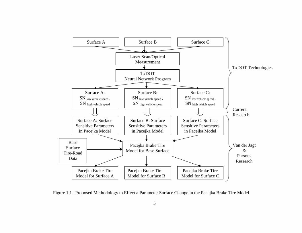
the technology will have the capacity to represent ribbed tire designs. A proposed

flowchart for a methodology to effect a parametric surface change in the Pacejka

Brake Tire Model that incorporates this future technology is presented in Figure 1.1.

Within the flowchart a skid number is denoted as SN.

5

Figure 1.1. Proposed Methodology to Effect a Parameter Surface Change in the Pacejka Brake Tire Model

Pacejka Brake Tire Model for Base Surface

Laser Scan/Optical Measurement

TxDOT Neural Network Program

Surface A: SN low vehicle speed , SN high vehicle speed

Surface C: SN low vehicle speed , SN high vehicle speed

Surface B: SN low vehicle speed , SN high vehicle speed

Surface A Surface B Surface C

Surface A: Surface Sensitive Parameters

in Pacejka Model

Surface C: Surface Sensitive Parameters

in Pacejka Model

Pacejka Brake Tire Model for Surface A

Pacejka Brake Tire Model for Surface C

Pacejka Brake Tire Model for Surface B

TxDOT Technologies

Current Research

Van der Jagt &

Parsons Research

Base Surface

Tire-Road Data

Surface B: Surface Sensitive Parameters

in Pacejka Model

6

1.3 Thesis Relevance

Empirical tire models are highly dependent on the particular surface for which

they were developed. The result of a more accurate tire-road interaction model

implies a better capacity for predicting how a vehicle will respond on a specific road

surface. With such a methodology, vehicle makers can improve and tune specific

component designs within a vehicle that are influenced by the tire-road interaction.

Whereas on the opposite side of the same “coin,” a road maker could begin to use this

methodology in conjunction with vehicle simulations to test surfaces against a

standard tire in order to determine safe driving conditions and or evaluate the quality

of a road surface. The ability to link these two engineering activities has been

discussed for many years, but its realization is a daunting task. This thesis takes a

small but positive step in this direction.

1.4 Thesis Presentation

This thesis is divided into five chapters. The first chapter presents the premise

and background of the thesis. The second chapter presents a review of friction, tire

mechanics and tire models relevant to this thesis. The third chapter presents a

standard method for which paved road surfaces may be classified and tested along

with the experimentation supporting this method. The fourth chapter presents a

methodology proposed for effecting a parametric surface change in a particular

empirical tire model called the Pacejka Tire Model [4]. The selection of this model

7

was not based on preferential treatment; rather the Pacejka Tire Model [4] is a

representation of a prototypical empirical tire model used in vehicle simulation. Both

chapters three and four include the relevant literature supporting the arguments made

in each of those chapters. The fifth chapter presents the conclusions of this thesis

along with recommendations for future work.

8

CHAPTER 2: Tire-Road Review

2.1 Introduction

This chapter presents three sections that review the current knowledge in

friction, tire mechanics, and tire models. These chapters only intend to relate the

necessary knowledge needed to understand the concepts and tools relevant in the

derivation of a road classification and test method for use in empirical tire models.

Each section provides a reference for the reader to locate if further knowledge on the

particular topic is desired. Each of these areas is the subject of a very extensive

literature base.

2.2 Friction

An understanding of the friction generated from a rolling tire on a road

surface is complicated and not yet fully understood [6]. However, a review of

friction’s origins in the literature, a brief description of rubber’s visco-elastic behavior

and the current representation of friction used to describe the interaction between the

tire and the road is presented in this section. This brief treatment of friction is

intended to motivate the discussion concerning tire-road friction and is in no way an

adequate overview of tribology, the study of friction, lubrication and wear. If more

information is needed concerning friction in general the reader is asked to reference

[7] for the state of the art in tribology.

9

2.2.1 Brief History of Friction

The mathematical description relating that the sliding force of one material

against another is proportional to the applied load times a constant material property

is universally called “Coulomb friction.” However, Coulomb (1736-1806), a French

physicist-engineer, was not the first to describe or investigate the relationship of the

friction force. While Coulomb considered friction to be due to the interlocking of

asperities, Amontons (1663-1705), also a French physicist-engineer, considered

friction to be the collision of surface irregularities and reached approximately the

same conclusion, namely Ffriction is proportional to Fnormal, nearly a century earlier in

1699. Both of these scientists asserted that the friction force was independent of the

area of contact between the two sliding surfaces. Coulomb went as far as to say that

he “discounted adhesion (which he called cohesion) as a source of friction and like

many others of his time considered the actual surfaces to be frictionless,” which

clearly contradicts modern theories of friction [7]. Nonetheless, Coulomb is

recognized with the dry friction approximation. In addition to these separate

descriptions of friction was the idea presented by the distinguished mathematician

Euler (1707-1783) who attributed the phenomenon of friction to hypothetical surface

ratchets. Later Samuel Vince (1749-1821) published a paper describing the static

friction of two materials as a function of both the kinetic friction and the adhesion

between those two materials. From this point on the subject of adhesion’s role in the

description of friction would be polemic. Leslie (1766-1832) argued against adhesion

by asserting that adhesion could not have an effect in a direction parallel to the

10

surface since adhesion is a force perpendicular to the surface [7]]. While Sir W.B.

Hardy argued that friction was due to molecular attraction operating across an

interfaces. Hardy also made another important distinction by asserting that the

molecular attraction operates over short distances, which in turn differentiates

between real area of contact and apparent area of contact. Tomlinson further tested

these ideas stating that the adhesion approach is based on the partial irreversibility of

the bonding force between atoms. The idea of adhesion, as the source of friction,

developed into the Adhesion Theory of Friction by the significant contributions made

by Beare, Bowden and Tabor. They found that friction is proportional to the true

contact area and the shear strength of the bonds in that area. They also recognized

that “the physical process occurring during sliding is too complicated to yield easily

to a simple mathematical treatment” [7]. This statement still persists today and can

be seen readily in complications arising from the description of visco-elastic materials

traversing quasi-rigid surfaces or better known as the tire-road friction problem.

2.2.2 Tire Visco-Elasticity and the Road Surface

Pneumatic tires are polymers. Specifically pneumatic tires are a combination

of rubber, carbon black, and oil. The additives of carbon black and oil improve wear

resistance and increase the overall friction between a tire and a road surface,

respectively. Polymers, in general, are visco-elastic, which means that they

mechanically appear to be elastic under high strain rates and viscous under low strain

rates [7]. This relationship is typically non linear and as such there are no simple

11

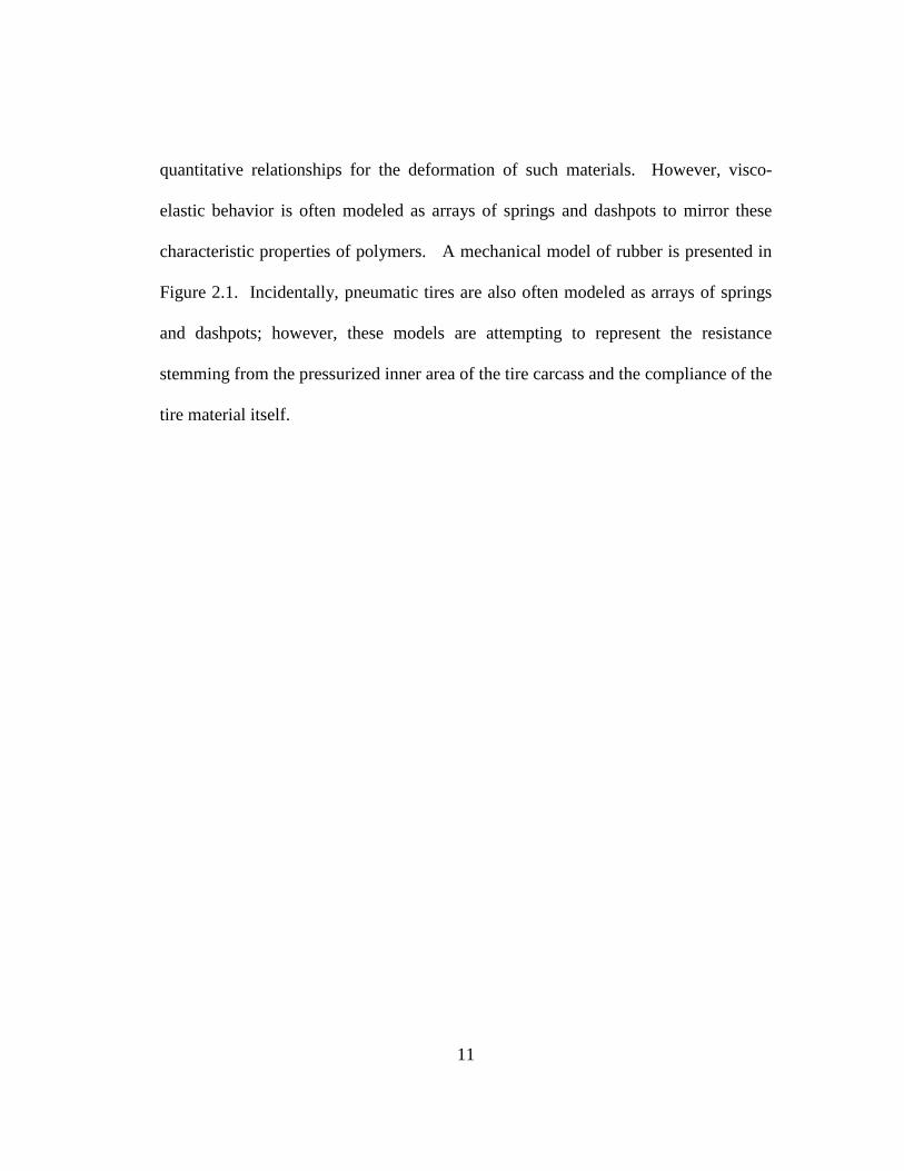
quantitative relationships for the deformation of such materials. However, visco-

elastic behavior is often modeled as arrays of springs and dashpots to mirror these

characteristic properties of polymers. A mechanical model of rubber is presented in

Figure 2.1. Incidentally, pneumatic tires are also often modeled as arrays of springs

and dashpots; however, these models are attempting to represent the resistance

stemming from the pressurized inner area of the tire carcass and the compliance of the

tire material itself.

12

Figure 2.1. Mechanical Model of Rubber

Input

Compliance (K)

Resistance (R)

Compliance (K)

13

A characteristic behavior of visco-elastic materials is their dependence on

strain rate and temperature. It has been well observed that the Young’s Modulus of

polymers decreases over time of loading, which is drastically different from the

plastic deformation of metals. If a pure rubber is given a laboratory sliding friction

test against a “smooth” surface in clean conditions, the frictional coefficient is found

to depend on the sliding speed and temperature. Curves for various temperatures can

be reduced to a single master curve using a Williams-Landel-Ferry (WLF)

transformation, which is based on the visco-elastic model of rubber. If the rubber

were then tested on a rough surface the WLF transformation would still be successful,

however, the master curve would take on a different shape. The new shape is due to

rubber distortion around the rough asperities, while the previous much smaller scale

molecular effects contributing to the friction are of diminished importance. Both

resultant master curves have a very strong correlation between the equations of visco-

elastic behavior and of rubber friction, which “suggest that at the very least the

phenomena have a common origin, and possible that the visco-elasticity is the cause

of rubber sliding friction” [7]. Additionally, these simple sliding friction tests point

out the importance surface geometry has in the development of friction between two

surfaces.

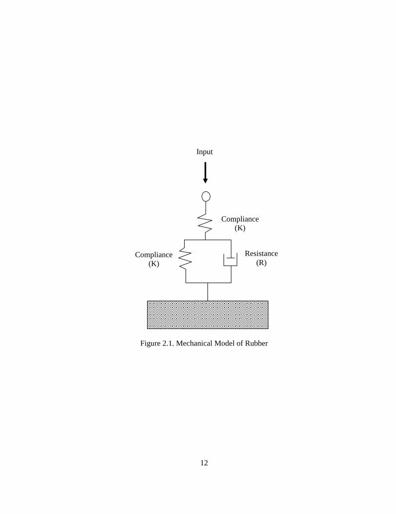
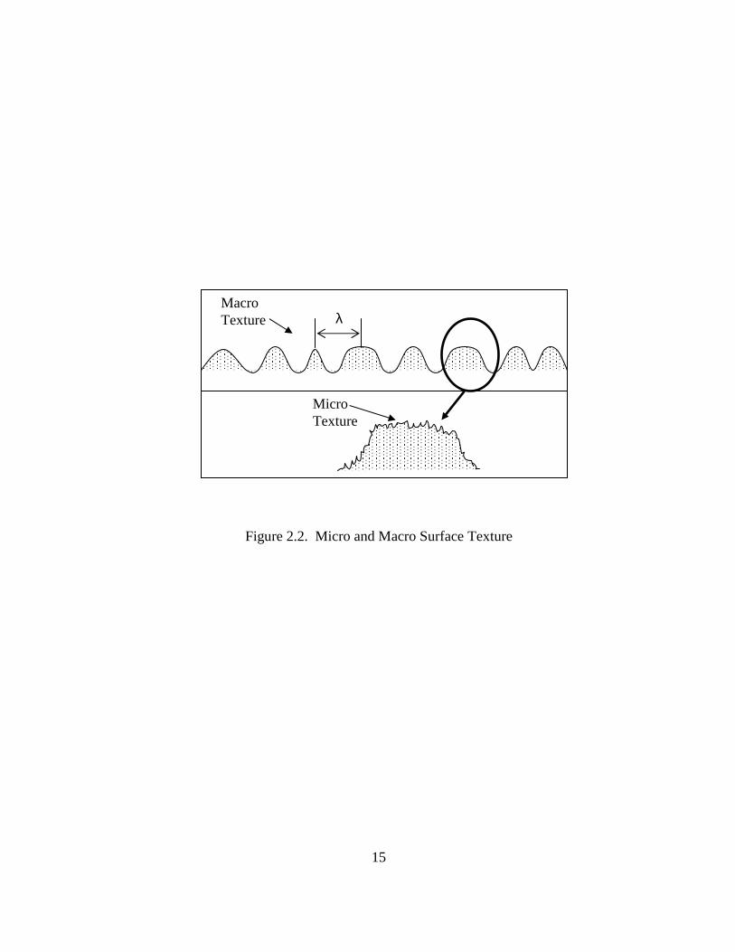
The geometry of a road surface has several scales that range from about 0.01

mm to 100.0 m in terms of wavelengths, a range of 10,000 to 1. Within this range

exist two dominant scales, classified as micro and macro texture, that greatly affect

the frictional development of a pneumatic tire and a road surface [8]. Macro texture

14

is a measure of the surface relief of a pavement, while micro-texture is a measure of

the degree of polishing of a pavement surface or of the aggregate at the surface [9].

In other words the individual asperities or stones in a road surface constitute the

macro-roughness, which range from 6 to 20 mm in size, while the geometry at the

tips of the asperities or stones constitutes the micro-texture, which range from 10 to

100 microns [8]. Figure 2.2 illustrates these two scales.

15

Figure 2.2. Micro and Macro Surface Texture

λ

Micro Texture

Macro Texture

16

2.2.3 Tire-Road Friction

The typical model used to describe a pneumatic tire sliding over a paved road

is based on the Adhesion Theory of Friction [10]. This model is often mislabeled as

the Coulomb Law of Friction. The Adhesion Theory of Friction owes much of its

development to Bowden and Tabor. The theory asserts that the force of friction,

Ffriction, is the product of the real area of contact, Ar, and the shear strength, Ss, of the

bond in that region. This relationship is mathematically described as,

Ffriction = Ar × Ss. (2.1)

The remaining part of the theory asserts that load, W, is the product of the average

pressure of contact, Pf, over the tips of the asperities that comprise an area of contact,

Ar, equivalent to the shear strength. This relationship is mathematically described as,

W = Ar × Pf. (2.2)

Together these relationships relate a ratio that has come to be known as the

coefficient of friction, µ, between two sliding surfaces. Thus altogether,

f

s

fr

srFriction

P

S

PA

SA

W

F===µ . (2.3)

Per this equation, µ is constant, independent of the vertical weight. However, the

friction phenomenon between rubber and solids does not necessarily obey the above

theory, namely because the theory is valid only for materials possessing a definite

yield point (such as metals) and it does not apply to elastic and visco-elastic materials

(such as rubber) [8]. In practice this theory is still used frequently as it presents a

17

simple quantitative expression for the sliding friction force in the absence of a

unifying theory for the rolling and sliding friction of visco-elastic materials on quasi-

rigid roads.

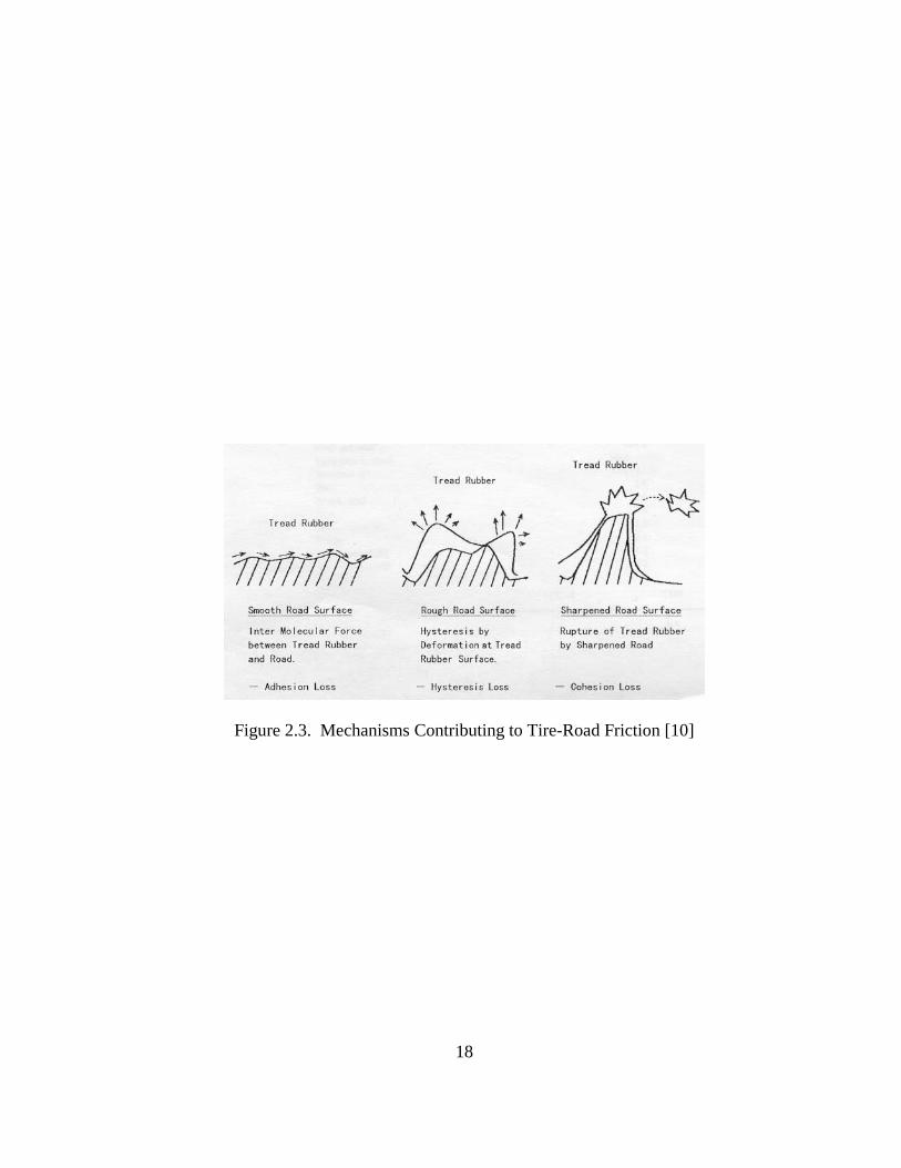
Currently three mechanisms are seen to contribute to the friction developed

between a pneumatic tire and a paved road: adhesion, hysteresis and cohesion [10].

Surface adhesion arises from the intermolecular bonds between the rubber and the

aggregate developed where the tire and road surface meet (commonly known as the

contact patch). The hysteresis mechanism represents energy loss in the rubber as it

deforms when sliding over the aggregate in the road at the contact patch. Cohesion

represents the rupture of tread rubber by sharp road asperities and is responsible for

wearing of the tire tread. Figure 2.3 [10] illustrates these three mechanisms.

18

Figure 2.3. Mechanisms Contributing to Tire-Road Friction [10]

19

2.3 Longitudinal Mechanics of Pneumatic Tire

The following section is a brief overview of the relevant knowledge required

to gain a physical understanding of the mechanics involved in the longitudinal motion

of a pneumatic tire. While the previous section concerned itself with describing the

sliding friction of objects, the following section will consider how friction plays a role

in vehicle dynamics when partially sliding, i.e. rolling. Since the information about

the mechanics of tires is quite extensive, further knowledge can be obtained from the

following references: [2] and [11].

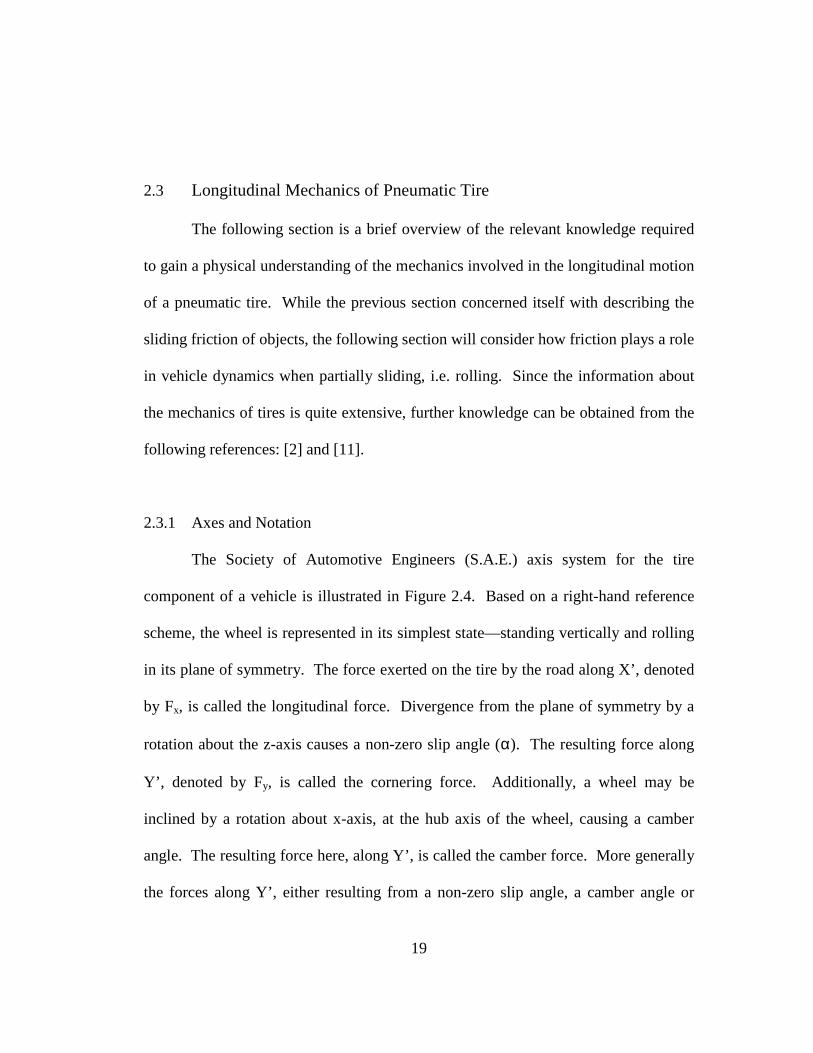
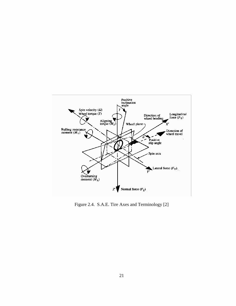
2.3.1 Axes and Notation

The Society of Automotive Engineers (S.A.E.) axis system for the tire

component of a vehicle is illustrated in Figure 2.4. Based on a right-hand reference

scheme, the wheel is represented in its simplest state—standing vertically and rolling

in its plane of symmetry. The force exerted on the tire by the road along X’, denoted

by Fx, is called the longitudinal force. Divergence from the plane of symmetry by a

rotation about the z-axis causes a non-zero slip angle (α). The resulting force along

Y’, denoted by Fy, is called the cornering force. Additionally, a wheel may be

inclined by a rotation about x-axis, at the hub axis of the wheel, causing a camber

angle. The resulting force here, along Y’, is called the camber force. More generally

the forces along Y’, either resulting from a non-zero slip angle, a camber angle or

20

both are called lateral forces. The force along negative Z’, denoted by Fz, is called

the normal force, which is typically comprised of the static or dynamic weight of a

vehicle. The aligning moment, Mz, and the overturning moment, Mx, act clockwise,

positive to their respective axes. Worth mentioning again, is that all the forces and

moments, mentioned thus far, are exerted by the road on the tire.

21

Figure 2.4. S.A.E. Tire Axes and Terminology [2]

22

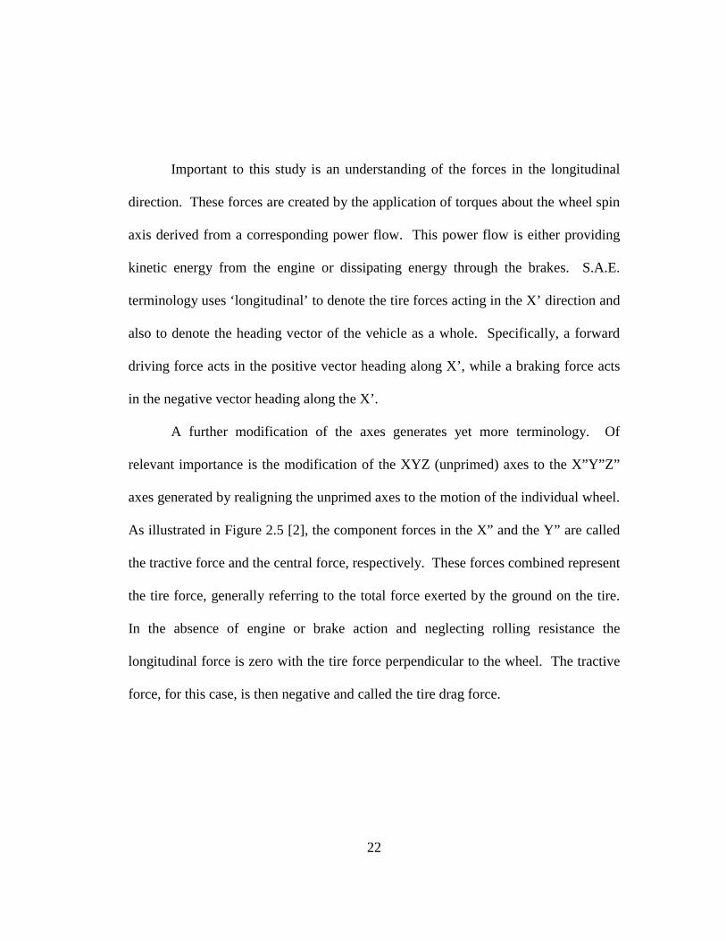
Important to this study is an understanding of the forces in the longitudinal

direction. These forces are created by the application of torques about the wheel spin

axis derived from a corresponding power flow. This power flow is either providing

kinetic energy from the engine or dissipating energy through the brakes. S.A.E.

terminology uses ‘longitudinal’ to denote the tire forces acting in the X’ direction and

also to denote the heading vector of the vehicle as a whole. Specifically, a forward

driving force acts in the positive vector heading along X’, while a braking force acts

in the negative vector heading along the X’.

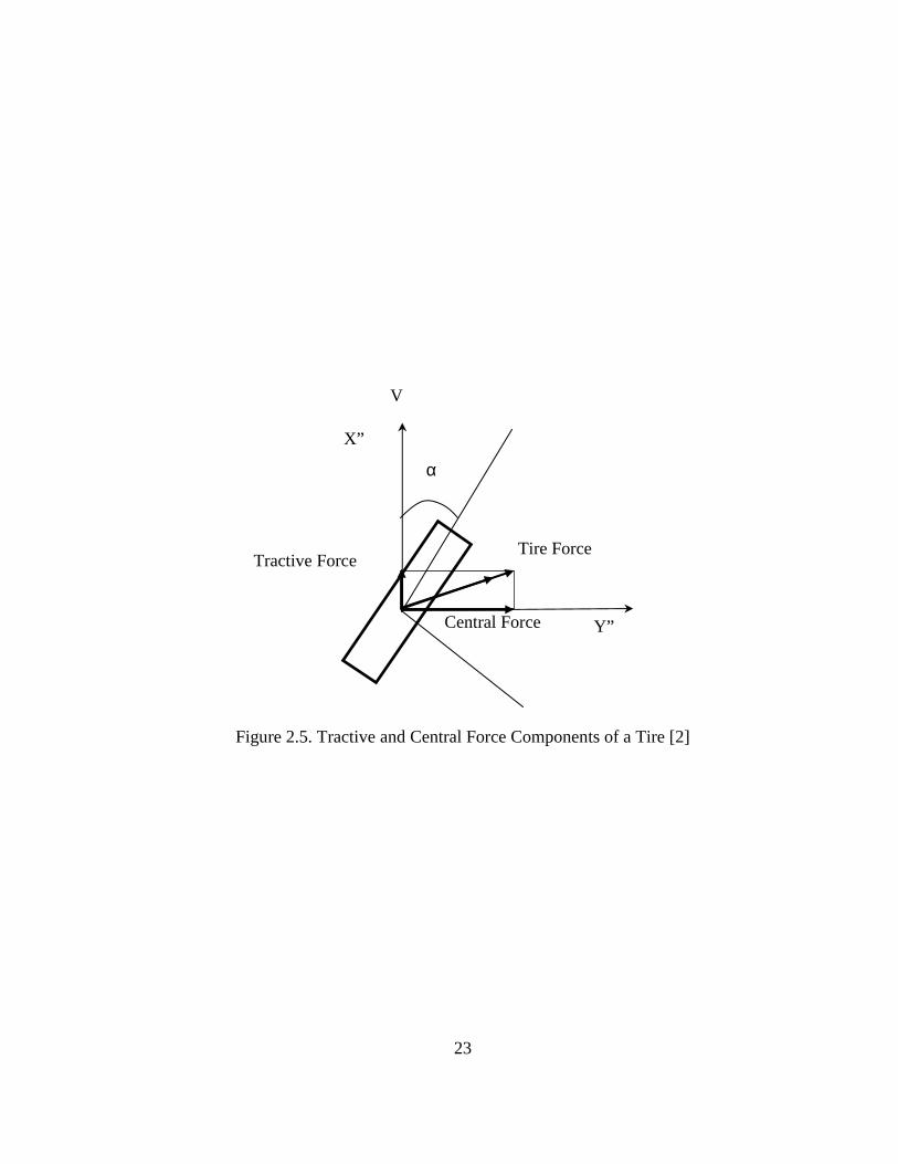
A further modification of the axes generates yet more terminology. Of

relevant importance is the modification of the XYZ (unprimed) axes to the X”Y”Z”

axes generated by realigning the unprimed axes to the motion of the individual wheel.

As illustrated in Figure 2.5 [2], the component forces in the X” and the Y” are called

the tractive force and the central force, respectively. These forces combined represent

the tire force, generally referring to the total force exerted by the ground on the tire.

In the absence of engine or brake action and neglecting rolling resistance the

longitudinal force is zero with the tire force perpendicular to the wheel. The tractive

force, for this case, is then negative and called the tire drag force.

23

Figure 2.5. Tractive and Central Force Components of a Tire [2]

V

α

X”

Y”

Tractive Force Tire Force

Central Force

24

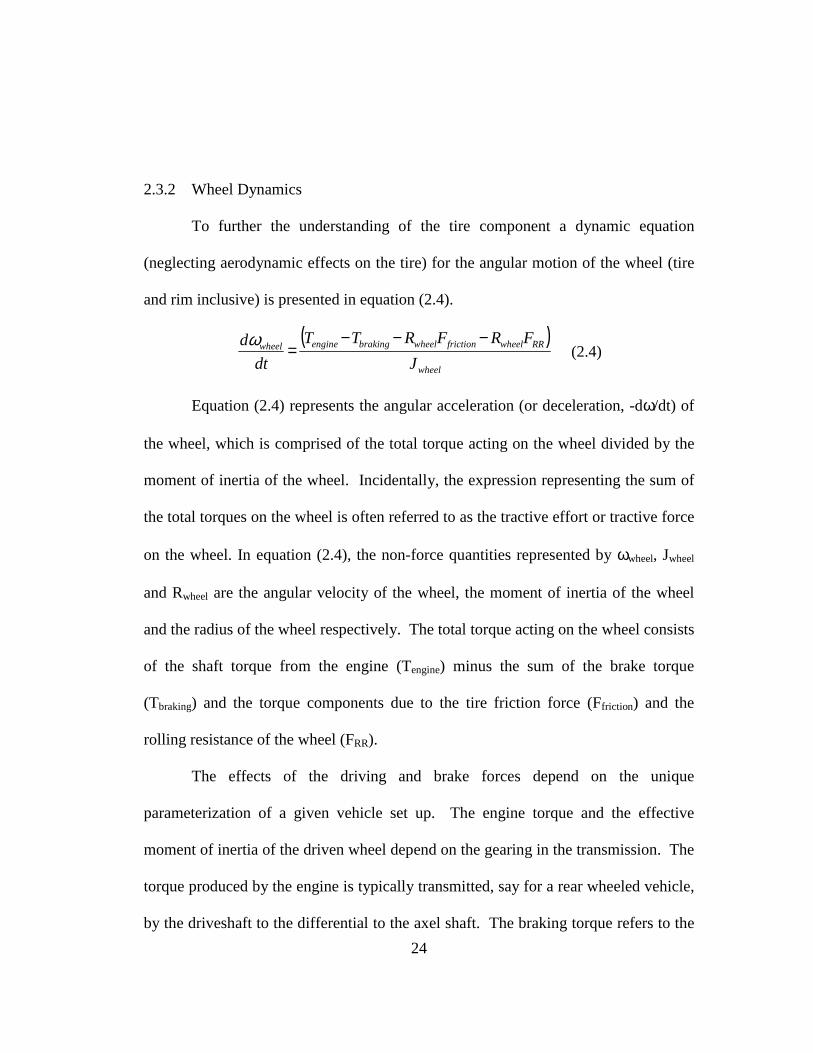
2.3.2 Wheel Dynamics

To further the understanding of the tire component a dynamic equation

(neglecting aerodynamic effects on the tire) for the angular motion of the wheel (tire

and rim inclusive) is presented in equation (2.4).

( )wheel

RRwheelfrictionwheelbrakingenginewheel

J

FRFRTT

dt

d −−−=ω

(2.4)

Equation (2.4) represents the angular acceleration (or deceleration, -dω/dt) of

the wheel, which is comprised of the total torque acting on the wheel divided by the

moment of inertia of the wheel. Incidentally, the expression representing the sum of

the total torques on the wheel is often referred to as the tractive effort or tractive force

on the wheel. In equation (2.4), the non-force quantities represented by ωwheel, Jwheel

and Rwheel are the angular velocity of the wheel, the moment of inertia of the wheel

and the radius of the wheel respectively. The total torque acting on the wheel consists

of the shaft torque from the engine (Tengine) minus the sum of the brake torque

(Tbraking) and the torque components due to the tire friction force (Ffriction) and the

rolling resistance of the wheel (FRR).

The effects of the driving and brake forces depend on the unique

parameterization of a given vehicle set up. The engine torque and the effective

moment of inertia of the driven wheel depend on the gearing in the transmission. The

torque produced by the engine is typically transmitted, say for a rear wheeled vehicle,

by the driveshaft to the differential to the axel shaft. The braking torque refers to the

25

actual application of either disc brakes or drum brakes. Depending on the brake

proportioning of a braking system, the vehicle actuates a mechanism (brake calipers

or a spring loaded resistor plate) to make contact with an adjacent plate rigidly

connected to the wheel inducing friction forces between the two moving surfaces to

dissipate energy.

On the other hand, the rolling resistance force and friction force depend on the

unique interrelationship between tire and road surface properties. The rolling

resistance, present from the instant the wheel begins to turn, depends on the

complicated and interdependent physical properties of the tire and ground that act to

dissipate energy from the tire. There are at least seven mechanisms, according to

[11], responsible for the rolling resistance of a tire. These mechanisms are: energy

loss due to the deflection of the tire sidewall near the contact area, energy loss due to

the deflection of the tread elements, scrubbing in the contact patch, tire slip in the

longitudinal and lateral directions, deflection of the road surface, air drag on the

inside and outside of the tire, and energy loss on bumps. It is also worth mentioning

that the energy lost by the tire material as a result of rolling resistance is converted

into heat within the tire, which subsequently reduces the abrasion resistance and the

flexure fatigue strength of the tire material [11]. The friction force is predominantly

due to three mechanisms: adhesion, hysteresis, and cohesion (see Section 2.2.3). Of

these, adhesion and hysteresis are most dominant. Both of these mechanisms depend

on some small wheel slip. The friction force can thus be said to be modulated by a

26

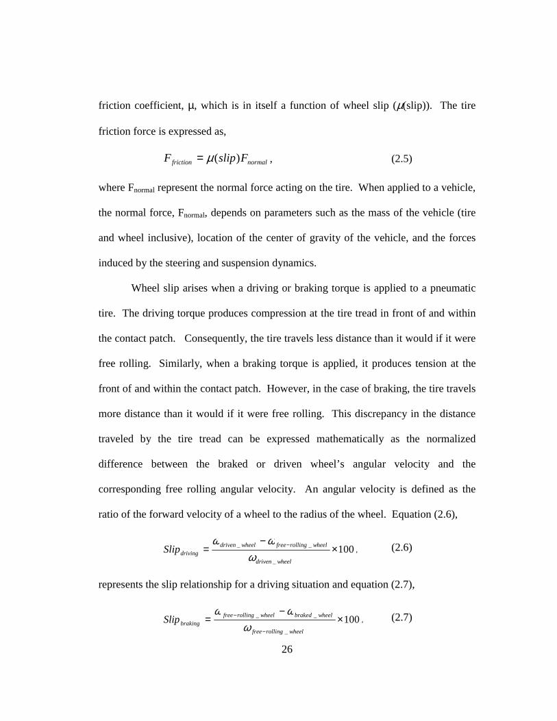
friction coefficient, µ, which is in itself a function of wheel slip (µ(slip)). The tire

friction force is expressed as,

normalfriction FslipF )(µ= , (2.5)

where Fnormal represent the normal force acting on the tire. When applied to a vehicle,

the normal force, Fnormal, depends on parameters such as the mass of the vehicle (tire

and wheel inclusive), location of the center of gravity of the vehicle, and the forces

induced by the steering and suspension dynamics.

Wheel slip arises when a driving or braking torque is applied to a pneumatic

tire. The driving torque produces compression at the tire tread in front of and within

the contact patch. Consequently, the tire travels less distance than it would if it were

free rolling. Similarly, when a braking torque is applied, it produces tension at the

front of and within the contact patch. However, in the case of braking, the tire travels

more distance than it would if it were free rolling. This discrepancy in the distance

traveled by the tire tread can be expressed mathematically as the normalized

difference between the braked or driven wheel’s angular velocity and the

corresponding free rolling angular velocity. An angular velocity is defined as the

ratio of the forward velocity of a wheel to the radius of the wheel. Equation (2.6),

100_

__ ×−

= −

wheeldriven

wheelrollingfreewheeldrivendrivingSlip

ωωω

, (2.6)

represents the slip relationship for a driving situation and equation (2.7),

100_

__ ×−

=−

−

wheelrollingfree

wheelbrakedwheelrollingfreebrakingSlip

ωωω

, (2.7)

27

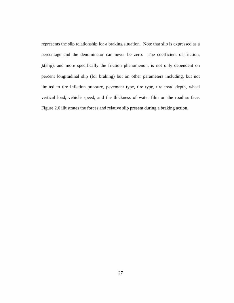
represents the slip relationship for a braking situation. Note that slip is expressed as a

percentage and the denominator can never be zero. The coefficient of friction,

µ(slip), and more specifically the friction phenomenon, is not only dependent on

percent longitudinal slip (for braking) but on other parameters including, but not

limited to tire inflation pressure, pavement type, tire type, tire tread depth, wheel

vertical load, vehicle speed, and the thickness of water film on the road surface.

Figure 2.6 illustrates the forces and relative slip present during a braking action.

28

ω

Contact Length

V

Relative Slip

r

Friction Force

Vertical Load

Figure 2.6. Braking Impact on the Tire [11]

29

The amount of braking force due to the hysteresis is controlled by the design

of the tire’s material properties, whereas the amount of adhesion produced is

controlled by both tire and road surface properties. Extreme cases of driving slip

present a situation where the tire is not moving directionally forward, it is merely

turning in place. The extreme case of braking slip presents a situation where the tire

is not rotating, it is merely skidding or sliding across the road directionally forward.

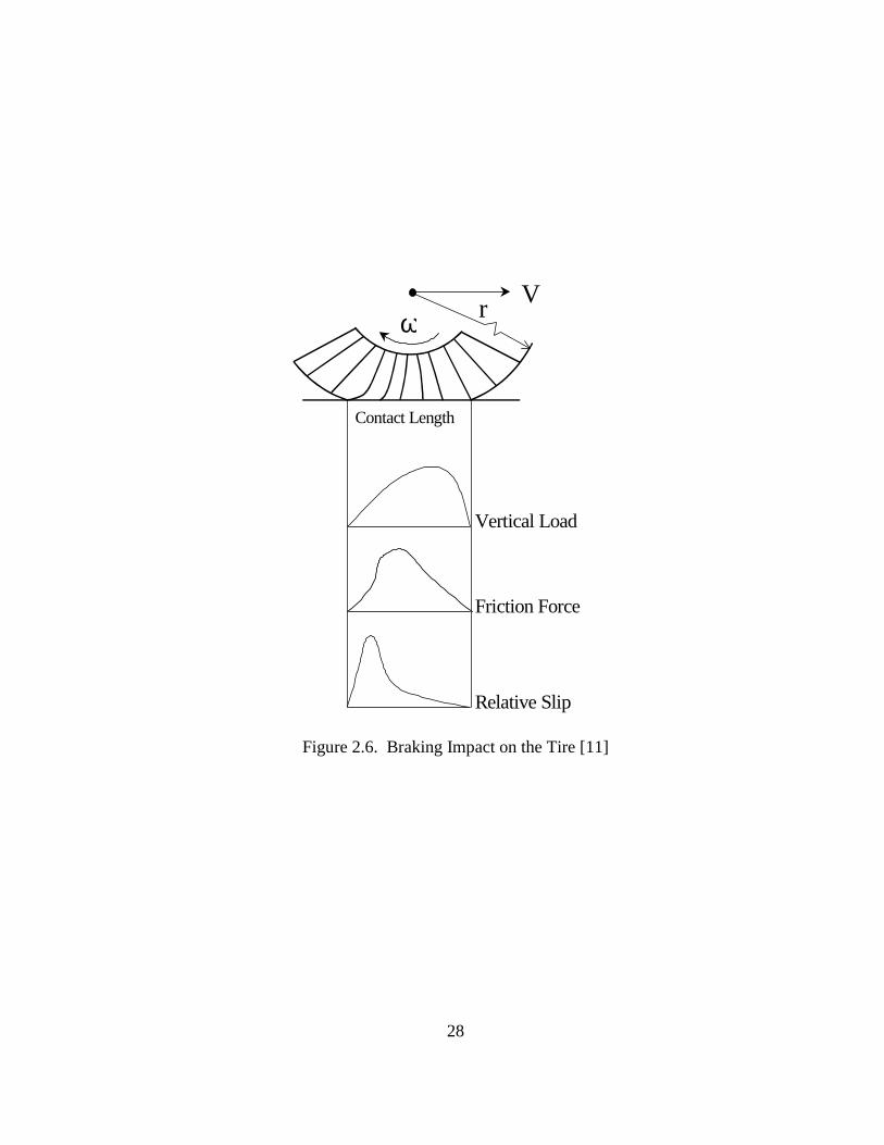
2.3.3 Braking Characteristics

Of particular importance to this investigation are the braking characteristics of

a pneumatic tire. An informed view on the parameters influencing the relationship

arising between the tire’s friction force and the percentage of slip allow for greater

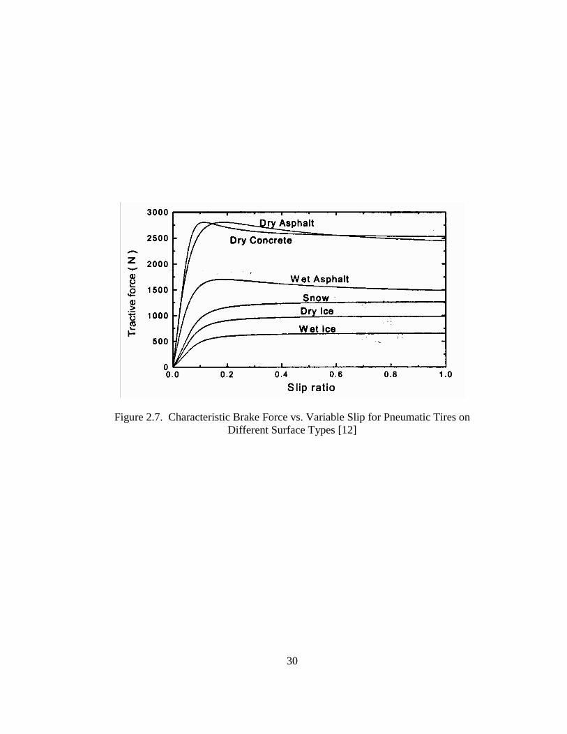
insight to the problem this thesis addresses. The braking force of a tire on a surface

changes non-linearly with slip. Various curves representing the characteristic brake

force versus slip trend on a variety of surfaces is presented below in Figure 2.7 [12].

30

Figure 2.7. Characteristic Brake Force vs. Variable Slip for Pneumatic Tires on Different Surface Types [12]

31

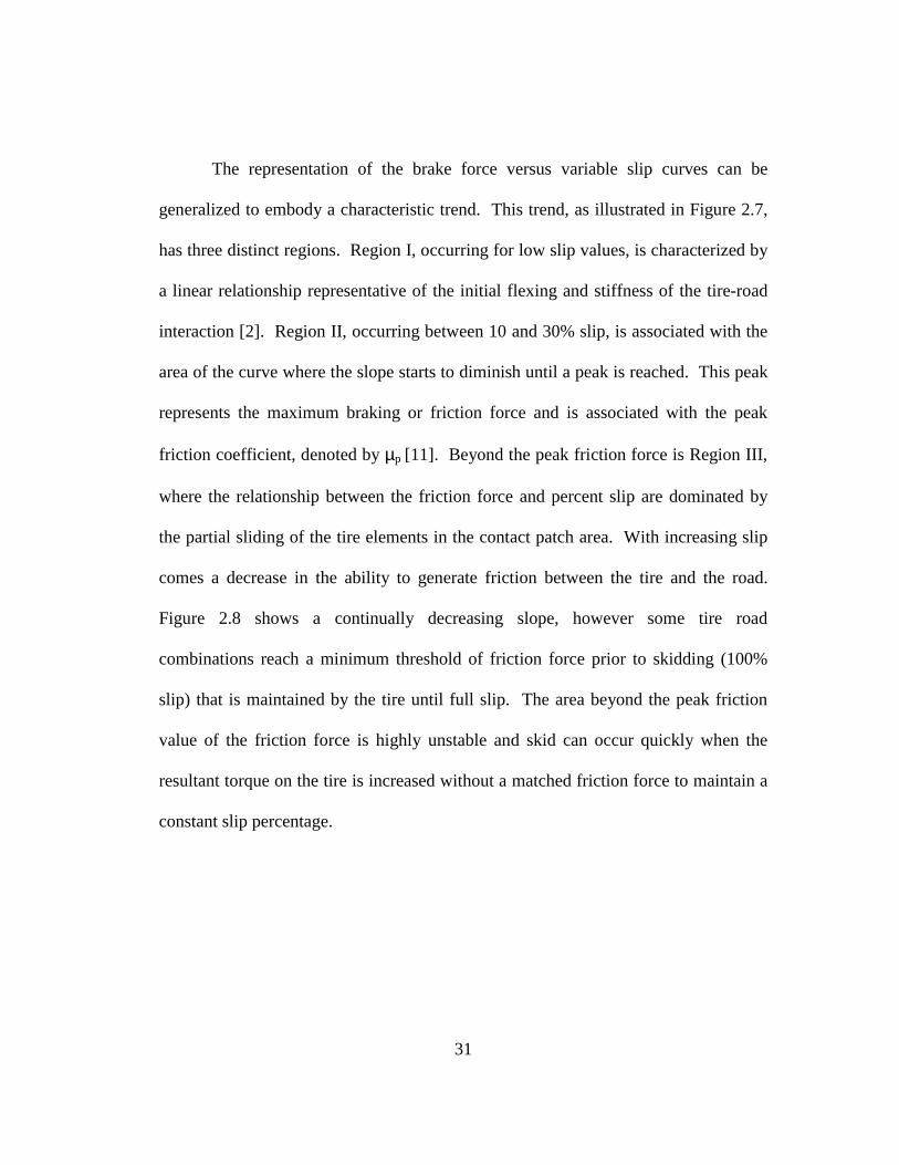
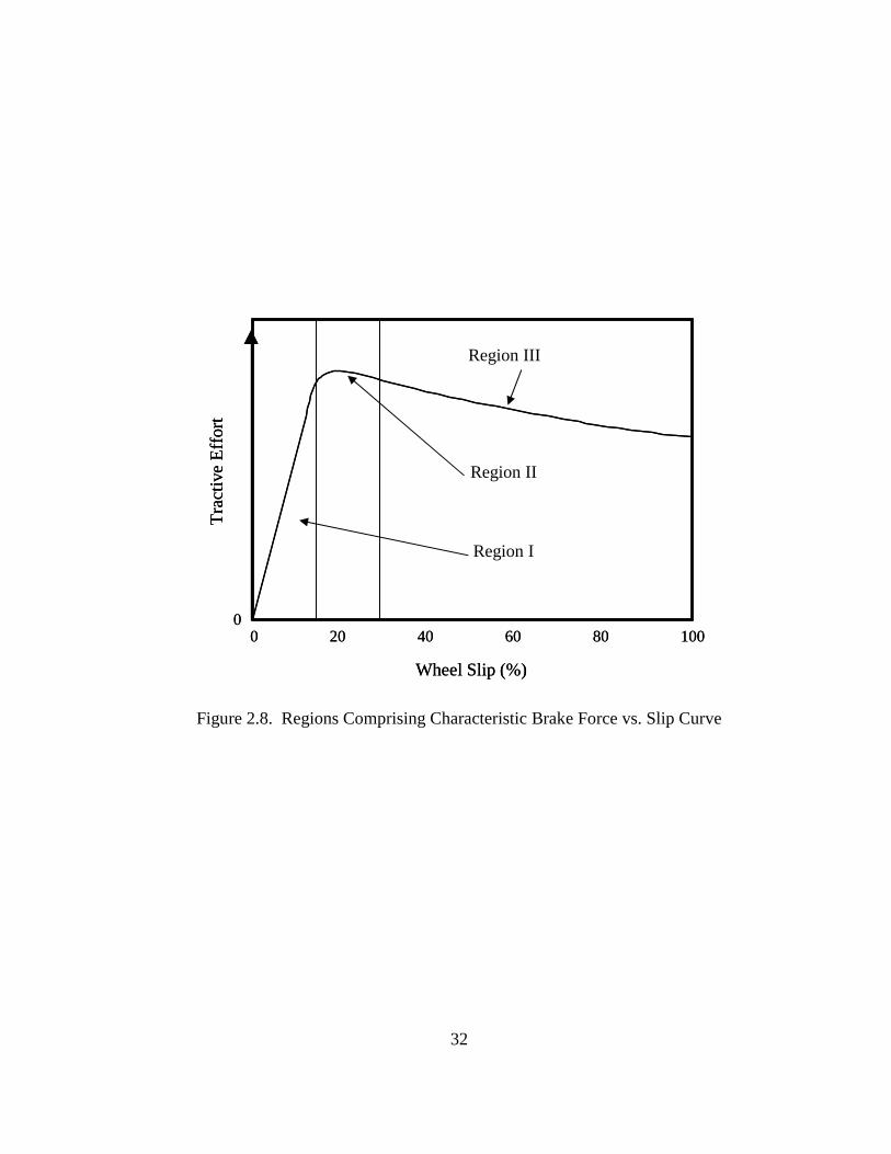
The representation of the brake force versus variable slip curves can be

generalized to embody a characteristic trend. This trend, as illustrated in Figure 2.7,

has three distinct regions. Region I, occurring for low slip values, is characterized by

a linear relationship representative of the initial flexing and stiffness of the tire-road

interaction [2]. Region II, occurring between 10 and 30% slip, is associated with the

area of the curve where the slope starts to diminish until a peak is reached. This peak

represents the maximum braking or friction force and is associated with the peak

friction coefficient, denoted by µp [11]. Beyond the peak friction force is Region III,

where the relationship between the friction force and percent slip are dominated by

the partial sliding of the tire elements in the contact patch area. With increasing slip

comes a decrease in the ability to generate friction between the tire and the road.

Figure 2.8 shows a continually decreasing slope, however some tire road

combinations reach a minimum threshold of friction force prior to skidding (100%

slip) that is maintained by the tire until full slip. The area beyond the peak friction

value of the friction force is highly unstable and skid can occur quickly when the

resultant torque on the tire is increased without a matched friction force to maintain a

constant slip percentage.

32

Wheel Slip (%)

0 20 40 60 80 1000

Tra

ctiv

e E

ffor

t

Wheel Slip (%)

0 20 40 60 80 1000

Tra

ctiv

e E

ffor

t

Figure 2.8. Regions Comprising Characteristic Brake Force vs. Slip Curve

Region I

Region II

Region III

33

2.4 Mathematical Tire Models

In general, mathematical tire models provide a construct within which some

physical aspect of the tire component system can be studied. The mathematical tire

models of importance to this thesis are those that relate the frictional force developed

between a pneumatic tire and a paved road surface. Moreover, it is the tire model that

can be easily incorporated into a vehicle simulation accurately and reliably to predict

the frictional force relationship that presents the best platform to investigate and

realize a tire model’s ability to adapt a surface variation. A brief review of the

literature representing the alternative methods used to model tires, a comparative

assessment of those models with respect to vehicle simulation, and a review of the

empirical tire model chosen, The Pacejka Tire Model [4], are presented in this

section.

2.4.1 Alternatives

There exist different types of tire models that aid the analysis of different

problems conducted by tire designers, vehicle dynamicist, and rolling contact

specialist [2]. For instance there are tire models that can inform on the dynamic

response of a tire, important when designing for ride comfort or noise reduction while

other tire models can predict the life expectancy of a tire, important when designing

for safety or warranty. The tire models relevant to a study focusing on the effects a

34

road surface has on the performance of a tire are those that relate the frictional forces

developed between a pneumatic tire and a paved road surface. In general, the

development of tire models can be categorized into one of the following types:

computational tire models (physically founded tire models that require computation

for their analysis), analytical tire models (physically founded tire models that allow

for analytic solutions), and empirical tire models (formula based tire models derived

by empirical methods). A brief synopsis of each type of model is provided and then a

review of a study [1] comparing the different modeling aspects of tire models for

vehicle simulation is presented. In essence the comparative study [1] found that

empirical tire models present the best opportunity to investigate the effects tires have

on vehicle dynamics within the framework of vehicle simulation.

2.4.1.1 Computational

Computational tire models, in general, are based on the viewpoint that the

mechanical behavior of the pneumatic tire is connected essentially to its deformation

resulting from the elastic and geometric properties of the carcass and inflation

pressure. The formulations predicting the shear force development depend on the

pressure that exists where the tire and pavement meet (contact patch) and on the

adhesion and sliding friction coefficients found therein. Computational tire models

involve extensive calculations but, because of the repetitive nature of these

computations, these models are ideally suited for programming within a computer

environment. Typically, computational tire models allow for a wide parameterization

35

of the design variables effecting a detailed representation of the tire structure and the

interactions of the tread with the ground [1]. Computational tire models are widely

used by tire manufactures for the structural design and analysis of the tire and have

presently been a platform on which the modeling of industrial tires (e.g. farm

equipment tires, tractor tires, etc…) traversing soft soil is being conducted. Finite

Element Method (FEM) and multi-spoke tire models are representative of the

computational tire models used in industry to relate the frictional forces developed

between a pneumatic tire and a paved road surface [1].

2.4.1.2 Analytical

Analytical tire models are based on the viewpoint that to sufficiently describe

the behavior of a tire only the dominant mechanisms present in the kinematics and

dynamics of a rolling deformable disc are needed. As such, analytical tire models are

quite idealized and simplified versions of the physical phenomenon they describe.

Analytical tire models were historically first developed to understand the basic

phenomenon related to the shear force and moment generating properties of the tire

[1]. Modern analytical tire models address a wide array of issues ranging from the

very focused model to a model describing the general behavior of the tire. The Brush

Tire Model and variations thereof is representative of the analytical tire models used

to relate the frictional forces developed between a pneumatic tire and a paved road

surface [1]. Analytical tire models, often called semi-empirical tire models,

parameterize the design variables using data acquired through full-scale

36

experimentation. Most analytical tire models are used to explain and obtain the

solution for very specific phenomenon resulting from specific operating conditions.

2.4.1.3 Empirical

Empirical tire models are based on the viewpoint that to realize the total

effects of the tire-road interaction, a mathematical fit to experimental data of an actual

tire operating in a real world environment is needed. Mathematical functions, such as

polynomials, exponential, arctangents, and hyperbolic tangent functions, are used to

fit the discrete experimental data with a continuous formulation representing the

behavior of a specific tire under specific operating conditions [1]. Modern empirical

tire models have the ability to capture the physical significance of some parameters

enabling vehicle designers a more fundamental appreciation for the mathematical

formulae [4]. Most empirical tire models are used to relate the dependence of design

parameters to the performance of a tire under actions of driving, braking or steering.

As such, empirical tire models are used extensively by both tire and vehicle design

engineers. The Pacejka Tire Model [4] and the Exponential Model [22] are

representative of the tire models found in industry today relating the frictional forces

developed between a pneumatic tire and a paved road surface.

2.4.2 Comparative Review for Vehicle Simulation

A standard to classify and test paved road surfaces with respect to their

frictional capacity with a particular tire cannot realize improving vehicle safety if it

37

cannot be integrated into the platform from which tires are designed and analyzed for

vehicle use. As such, the tire model chosen is crucial to the process of realizing

improved vehicle safety. A recent study, by R.S. Sharp and H.B. Pacejka [1],

compared and reviewed the extensive research and technologies developed for

computational, analytical, and empirical tire models. The study [1] focused on

models dealing with the shear (friction) force development of a tire on a road surface.

A specific result of the study [1] identified empirical tire models to be the most

suitable platform to investigate a tire’s influence on the response of a vehicle in a

dynamic simulation environment.

Criteria were developed in [1] to compare a tire model’s usefulness to vehicle

simulation studies. The criteria considered accuracy, range of behavior, number of

parameters, physical significance of the parameters, the ease by which the parameters

and data could be obtained, the capability and simplicity to cover behavior outside the

range of working conditions used for parameter evaluation, and the computation load

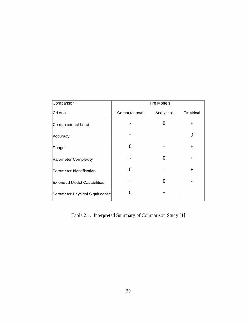
(time and resources required). The comparative study [1] subsequently described the

main physical features and ideas of those models from the literature “which appear to

have the most advantageous combinations of properties” in areas of computational,

analytical, and empirical tire model development. Table 2.1 presents an interpreted

summary of the results found in the comparative study [1], since there was no formal

graphical presentation of the results. To create Table 2.1 three subjective rankings

were developed to relate the information found in the study [1]. A plus (+) ranking

indicates a benefit to the tire model, a minus (–) ranking indicates a disadvantage of

38

the model, and a zero (0) ranking indicates a nominal feature in comparison to the

other tire models.

39

Comparison Tire Models

Criteria Computational Analytical Empirical

Computational Load - 0 +

Accuracy + - 0

Range 0 - +

Parameter Complexity - 0 +

Parameter Identification 0 - +

Extended Model Capabilities + 0 -

Parameter Physical Significance 0 + -

Table 2.1. Interpreted Summary of Comparison Study [1]

40

The comparative study [1] identified that computational tire models are

powerful in terms of accuracy and extended capabilities given their explicit physical

modeling. However, computational tire models encounter “significant penalty in

terms of computational load, which make them an unlikely candidate to provide a

basis for dealing with the tire forces in a vehicle simulation” [1]. Additionally, the

comparative study [1] identified that the strength of analytical tire models,

representing the tire in vehicle dynamic studies, lies in “their good representation of

the basic geometry of rolling distributed contact and the competition between elastic

forces and friction forces showing qualitatively reasonable correspondence with

experimentally found tire characteristics” [1]. However, the comparative study

found that the required simplification of the physical phenomenon and the difficulty

obtaining suitable values for the parameterization of analytical tire models limit their

ability to adequately describe the behavior of the tire for vehicle dynamic studies and

subsequently advise against their use. Finally, the comparative study [1] identified

that the strength of empirical tire model’s lie in their inherent ability (through the

mathematical fit of experimental data) to fully capture the physical phenomenon

resulting from the interaction of a tire with a road surface. Though paradoxically, it is

the specificity of empirical tire models that give it their greatest shortcomings. Using

a mathematical fit to experimental data greatly limits the physical significance of the

variables that make up an empirical tire model. Consequently, a parameterization,

changing one or more operating conditions (e.g. changing tire material, tire structure

properties, air pressure, road surface, vehicle speed, etc.) of an existing empirical tire

41

model often requires a new tire model to be formed from new experimental data

reflecting the change in operating conditions. Withstanding, the comparative study

[1] finds that tire models formed using empirical methods provide the most pragmatic

platform to pursue tire studies for vehicle simulation.

Without question the complexity of the pneumatic tire and its effects on

vehicle dynamics demands simplification. The tire is a multi-layered, non-uniform,

anisotropic, visco-elastic material interacting with a quasi-rigid road, whose

properties continually change according to local environmental conditions, use and

maintenance [2]. To overcome such complexities tire models are formed to address

specific issues pertaining to the tire component system. It is the tire model whose

specific objective is to relate the shear force development between a pneumatic tire

and a paved road surface that is of importance when seeking to quantify the effects a

surface variation has on the tire forces generated in a vehicle simulation. The

comparative study [1], reviewed in this section, provides the basis for choosing an

empirical tire model as the platform to investigate surface variation to ultimately

provide a more descriptive vehicle simulation. However, in the future, as computing

speeds, computing techniques, and more accurate tire mechanics continue to evolve,

computational and analytical tire models may potentially provide a better platform to

describe the shear force development of a pneumatic tire on a road surface for vehicle

simulation. The empirical tire model chosen for this investigation is the Pacejka Tire

Model [4].

42

2.4.3 The Pacejka Tire Model

Like many engineering technologies, the Pacejka Tire Model [4] is the

product of a demand—to improve vehicle safety. Specifically, the authors of the

Pacejka Tire Model wanted to address the growing field of dynamic safety by

introducing a comprehensive description of a tire’s behavior, where the safety of a

vehicle could be realized after optimizing stability, steering and brake performance by

tuning the chassis design to each other. The Pacejka Tire Model is based on the

empirical method of fitting formulae containing special functions to experimental

data. The basic formulation encompasses a model representing the longitudinal force

under pure braking, the lateral (side) force under pure cornering, and the self-aligning

torque under pure cornering. The basic Pacejka Tire Model has since evolved to

describe the tire horizontal force generation at combined slip [14] and the non-steady-

state behavior of the aligning torque [13]. The particular structure of the Pacejka Tire

Model provides great accuracy in describing the measured data and contains a few

parameters related to physically identifiable quantities in a simple manner. This

section provides an explanation of the Pacejka Brake Tire Model [4].

2.4.3.1 Formulation of Pacejka Brake Tire Model

The Pacejka Tire Model’s formulation is remarkably similar for the three

cases of longitudinal (brake) force versus slip, lateral (side) force versus slip angle

and aligning torque versus slip angle. The basic formulation of the Pacejka Tire

43

Model was first presented in a 1987 SAE paper titled “A New Tire Model with an

application on Vehicle Dynamic Studies,” by H. B. Pacejka, E. Bakker and L. Lidner.

The formulation of the Pacejka Brake Tire Model describes a tire’s steady

state behavior traveling over a dry hard smooth surface under the vehicle action of

pure braking [4]. The brake tire model cannot deal with road surface irregularities of

high frequencies, such as road bumps, or off road (soft soil) conditions. Furthermore,

and in general, suspension design parameters (such as camber angle and inflation

pressure), and operating conditions (such as type of road surface, vehicle speed, and

ambient temperature) must be set in advance of the collection of experimental data.

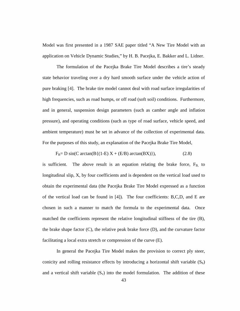
For the purposes of this study, an explanation of the Pacejka Brake Tire Model,

FB= D sin(C arctan(B{(1-E) X + (E/B) arctan(BX)}), (2.8)

is sufficient. The above result is an equation relating the brake force, FB, to

longitudinal slip, X, by four coefficients and is dependent on the vertical load used to

obtain the experimental data (the Pacejka Brake Tire Model expressed as a function

of the vertical load can be found in [4]). The four coefficients: B,C,D, and E are

chosen in such a manner to match the formula to the experimental data. Once

matched the coefficients represent the relative longitudinal stiffness of the tire (B),

the brake shape factor (C), the relative peak brake force (D), and the curvature factor

facilitating a local extra stretch or compression of the curve (E).

In general the Pacejka Tire Model makes the provision to correct ply steer,

conicity and rolling resistance effects by introducing a horizontal shift variable (Sh)

and a vertical shift variable (Sv) into the model formulation. The addition of these

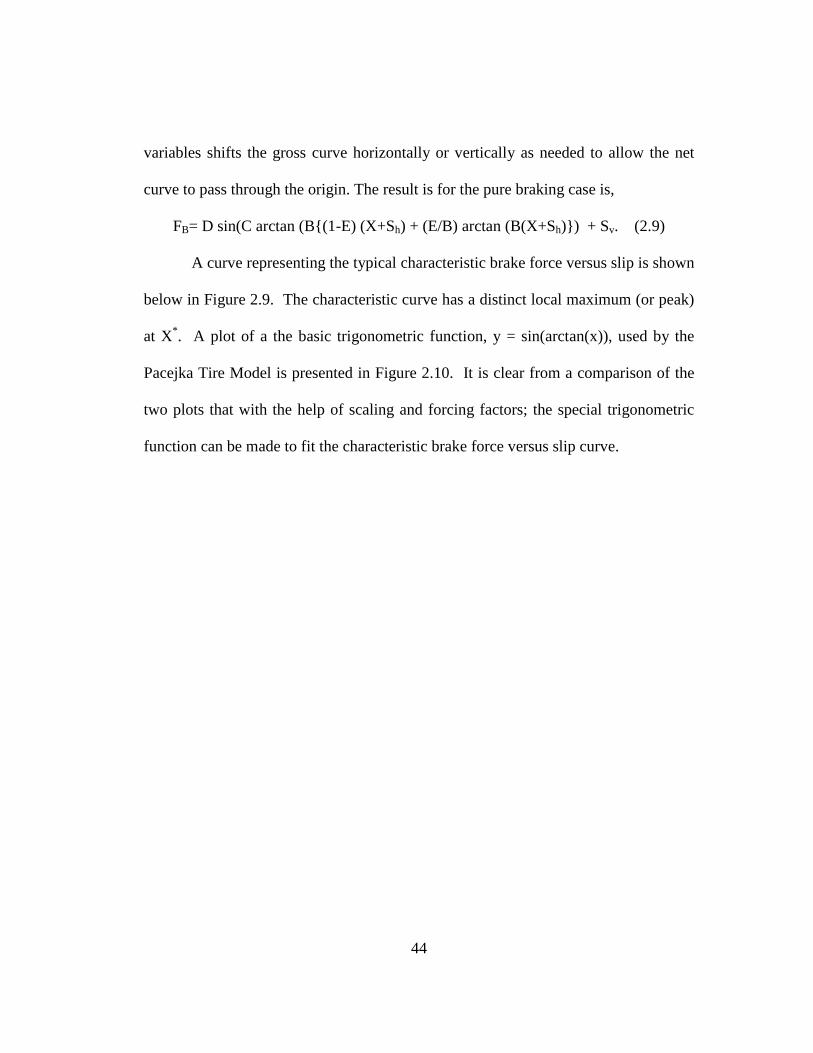
44

variables shifts the gross curve horizontally or vertically as needed to allow the net

curve to pass through the origin. The result is for the pure braking case is,

FB= D sin(C arctan (B{(1-E) (X+Sh) + (E/B) arctan (B(X+Sh)}) + Sv. (2.9)

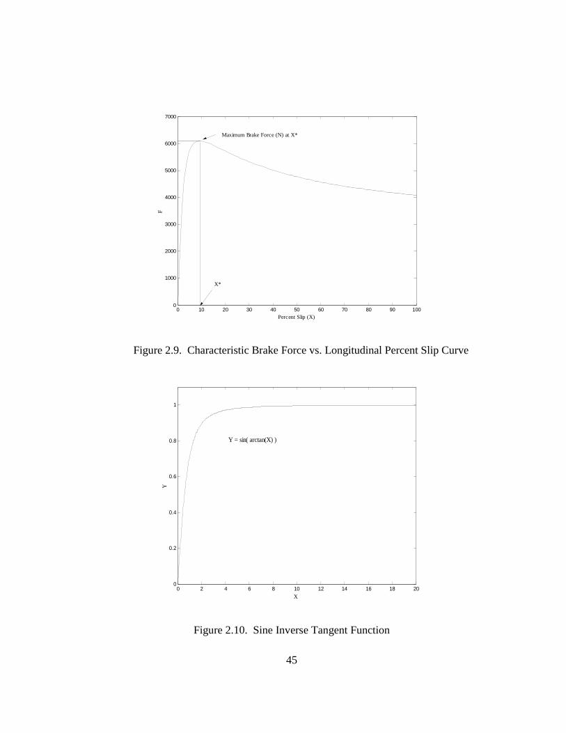
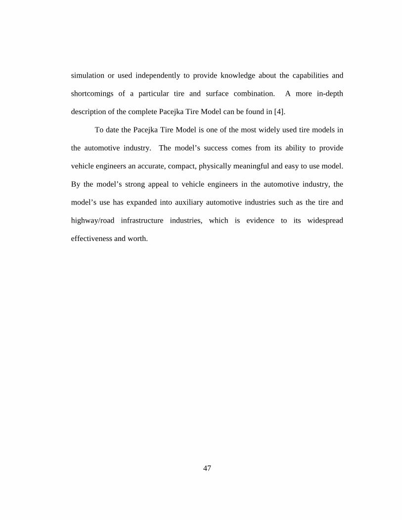
A curve representing the typical characteristic brake force versus slip is shown

below in Figure 2.9. The characteristic curve has a distinct local maximum (or peak)

at X*. A plot of a the basic trigonometric function, y = sin(arctan(x)), used by the

Pacejka Tire Model is presented in Figure 2.10. It is clear from a comparison of the

two plots that with the help of scaling and forcing factors; the special trigonometric

function can be made to fit the characteristic brake force versus slip curve.

45

0 10 20 30 40 50 60 70 80 90 1000

1000

2000

3000

4000

5000

6000

7000

Percent Slip (X)

F

Maximum Brake Force (N) at X*

X*

Figure 2.9. Characteristic Brake Force vs. Longitudinal Percent Slip Curve

0 2 4 6 8 10 12 14 16 18 200

0.2

0.4

0.6

0.8

1

X

Y

Y = sin( arctan(X) )

Figure 2.10. Sine Inverse Tangent Function

46

2.4.3.2 Generating a Pacejka Brake Tire Model

The basis for any Pacejka Tire Model is a full-scale test of the force and

moment response of a tire under the actions of either pure braking or cornering. To

obtain experimental brake force data, the force or pressure applied to the braking

mechanism of a tire is gradually increased beginning at a constant vehicle speed. The

brake force and longitudinal slip are continually measured at discrete increments from

a free rolling (no brake) condition to a lockup condition, 100% slip or skidding.

After the brake force versus slip data is obtained, a Pacejka Brake Tire Model

can be generated. A fitting process using the variables B, C, D, E and if necessary Sh,

and Sv are used to match the trigonometric function with the experimental data.

Incidentally, the brake shape factor, C, which controls the brake characteristic trend

of the curve, is typically 1.65. The value for the brake shape factor, C, has been

established through extensive modeling of tires. Also the value associated with the

vertical shift variable, Sv, typically accounts for the rolling resistance. Using a base

Pacejka Brake Tire Model to work from often facilitates the acquisition of the

coefficients and the two shifts variables. However, more refined techniques have

been developed to process the coefficients and shift values using optimization

schemes [4] and more recently a software package called Tyre Gene was released by

Yearstretch Limited that uses a genetic algorithm to obtain the coefficients.

Once a Pacejka Brake Tire Model is established, it can then be integrated into

a vehicle simulation program, such as Carsim, PNGV Systems Analysis Toolkit

(PNGVSAT), DADS or ADAMS to provide the necessary force input for vehicle

47

simulation or used independently to provide knowledge about the capabilities and

shortcomings of a particular tire and surface combination. A more in-depth

description of the complete Pacejka Tire Model can be found in [4].

To date the Pacejka Tire Model is one of the most widely used tire models in

the automotive industry. The model’s success comes from its ability to provide

vehicle engineers an accurate, compact, physically meaningful and easy to use model.

By the model’s strong appeal to vehicle engineers in the automotive industry, the

model’s use has expanded into auxiliary automotive industries such as the tire and

highway/road infrastructure industries, which is evidence to its widespread

effectiveness and worth.

48

CHAPTER 3: Road Classification and Test Method

3.1 Introduction

The following chapter presents the research and experimentation conducted in

support of the hypothesis presented in Chapter 1 of this thesis. The hypothesis states,

in essence, that a road surface can be identified and subsequently categorized by two

skid resistance tests, conducted at low and high vehicle speeds. The method used to

classify and test a road surface is developed anticipating its use in assisting the

adjustment of empirical tire models to a road surface variation. The development of

the road classification and test method is presented in Section 3.2. The

experimentation supporting the road classification and test method is presented in

Section 3.3.

3.2 Development of Paved Road Classification Method

The following sections present the argument and supporting literature for

using low and high vehicle speed skid resistance tests to identify and classify a road

surface. Presented as a derivation beginning with the main variables affecting

longitudinal braking, skid resistance tests at low and high vehicle speeds are shown to

represent the dominant surface characteristics contributing to the development of the

friction force between a road surface and a pneumatic tire.

49

3.2.1 Main Variables Affecting Longitudinal Braking

The characteristics of the frictional force developed between a pneumatic tire

and a road surface are a result of driving, steering, and braking actions applied to a

vehicle. The friction force resulting from the braking of a pneumatic tire traveling

along a paved road surface is in itself a result of many variables acting in concert.

The main independent variables affecting longitudinal tire braking, FB, according to

[15], can be expressed in equation form as,

FB = fcn{Tire Type, Tire Tread Depth, Inflation Pressure, (3.1)

Pavement Type, Wheel Vertical Load, Vehicle Speed,

Water Film Thickness, Operation Temperature,

Longitudinal Slip}.

The combination of these variables represents a system having at least nine degrees of

freedom. The effects of these independent variables and their interdependent

relationships are not completely understood [6]. However, the voluminous material

available in this research area indicates these variables can be studied to formulate an

understanding of their effects on tire-road dynamics.

3.2.2 Dominant Surface Properties Affecting Longitudinal Braking

This section reduces the main variables affecting longitudinal braking,

presented in Section 3.2.1, to two geometric surface properties. The following

presents the supporting literature for the preceding argument.

50

To fully realize the specific effects a pavement has on the frictional forces

generated under a pure braking action, all variables, excluding Pavement Type, must

be constrained or held constant. Imposing this requirement on (3.1) gives rise to,

FB[constant parameters] =fcn{Pavement Type}. (3.2)

Furthermore if (3.2), which is essentially a skid resistance test when conducted at

100% longitudinal slip, is expanded to include the constituent properties that

represent a Pavement Type [17] it will give rise to,

FB[constant parameters]=fcn{Type, Binder, Aggregate, (3.3)

Pavement Texture, Roughness, Topography}.

The expanded form of (3.2) presented in (3.3) excludes those variables pertaining to

road design (e.g. curve, grade, tangent, crown, etc.) as their impact is more readily

seen at the full vehicle system scale.

Expression (3.3) includes Pavement Texture, which is “perhaps the most

important single variable determining the magnitude of the friction forces between

tire and road” [8]. It is therefore asserted that the geometry of a surface dictates the

frictional development between a tire and a road surface and not the Aggregate, Type,

Binder, of the road. These properties of the road have “little effect because of the

great difference in hardness between tire rubber and road materials” [17]. Roughness

and Topography do not significantly contribute to tire road interaction as the effects

of Roughness are governed by the dynamic effect caused by the imbalances in the

drive train from surface geometry ranging from 0.1 m to 10 m [16], whereas

topography refers to the more regional effects of climate and regional disposition (e.g.

51

hills, planes, mountains) that effect the interaction of the tire and road on a more

systems level. Thus Pavement Texture, and in specific micro and macro texture are

seen as the two most influential scales of Pavement Texture contributing to the

development of the friction force between a tire and a road surface [8]. See Section

2.2.2 for a more detailed description of micro and macro texture.

It is now possible to re-write expression (3.3) from the above perspective to

formulate an expression for the braking force of a tire as a function of the micro and

macro texture properties of the pavement,

FB[constant and negligible parameters] = fcn{Micro Texture, MacroTexture}. (3.4)

Equation (3.4) represents a relationship in which the magnitude of the brake force is a

function of the micro and macro texture of a road surface. Equation (3.4) is possible

only if Tire Type, Tire Tread Depth, Inflation Pressure, Wheel Vertical Load, Vehicle

Speed, Water Film Thickness, Operation Temperature, and Longitudinal Slip are not

varied, and the effects of Type, Binder, Aggregate, Roughness, and Topography are

considered negligible in relation to Texture as asserted by [8] and [17].

It is worth noting that the aforementioned constraints imposed to a braking

maneuver are representative of those placed on skid resistance tests. In addition, the

constraint of maintaining Water Film Thickness constant in equation (3.4) does not

restrict it to be any value in particular, only that it must be maintained constant. This

observation provides significant ramifications as it can be construed, at least

theoretically, that with knowledge of the amount of water present in the contact patch,

52

water as a parameter can be quantified and related back to the brake or friction force

developed between a road surface and a pneumatic tire.

3.3 Development of Paved Road Test Method

Equation (3.2), presented in section 3.2.2, prescribes a braking action as a

function of Pavement Type whose required constraints are similar to a standardized

road test procedure called Skid Resistance Testing. The literature [9] supports that

when conducted at both low and high vehicle speeds these tests are indicative of a

surface’s micro and macro texture. Moreover, as it will be shown in this section,

when the vehicle speeds are chosen appropriately, the low vehicle speed skid test can

give a relative measure of the maximum braking (or peak friction) force of a vehicle

traveling at a speed coinciding with speed for the high vehicle speed skid test. The

use of these two values is central in classifying and testing road surfaces to estimate

the characteristic brake force versus slip curve and subsequently to facilitate the

adjustment of an empirical tire model to a surface variation.

Skid resistance tests, in the United States and abroad, are typically conducted

by road makers at high vehicle speeds on wet roads to assess the wet-pavement

traction of road surfaces. These tests are carried out with the more hazardous road

conditions in mind—a car skidding (100% slip) at high velocities (40-50 mph) on wet

surfaces (nominal water depth of 0.15 inches) [6]. Research into models predicting

the dependence of the friction force on water film thickness and vehicle speed is

53

ongoing with promising studies already present [18]. However, for the purposes of

developing a test method to evaluate the friction performance of a tire on a road

surface, it must be made clear whether the tests reflect dry or wet road conditions, and

if wet roads are prescribed the thickness of the water film applied during testing must

be stated. Thus the Water Film Thickness used while testing a particular tire will

delineate the classification of road surfaces by skid resistance tests into different

categories. The preceding can be asserted for two reasons. First, under wet road

conditions the characteristic brake force versus slip shape (see Section 2.3.3) is still

retained, only categorically (with respect to slip) diminished due to the lower overall

contribution of adhesion to the friction force [11]. Second, irrespective of whether a

skid resistance tests is performed on a dry or wet surface, the results of these test still

relate a ratio of the friction force to the normal force. When a standard tire and

standard test conditions are utilized in a measurement of pavement traction, the

results are reported as the skid number (SN) of the pavement as a function of vehicle

test speed (V),

SNv= (Ffriction/Fnormal) × 100, (3.5)

or alternatively,

SNv= (µ) × 100. (3.6)

“Skid resistance is therefore a pavement characteristic and is a function of the surface

properties, which can be modified by the presence of contaminants” [6].

54

The speed dependence of the skid number determines whether micro texture

or macro texture is being evaluated. To be certain, “micro texture is predominate in

determining the skid resistance of a road surface at low vehicle speeds (up to about 50

km/h),” while “macro texture is predominant in determining how well the skid

resistance of a road is maintained as the vehicle speed increases” [9]. This qualitative

assessment of the speed dependence of the skid number is present in both dry and wet

road surface conditions, but more pronounced under wet conditions. Central to the

use of skid numbers for the classification of road surfaces is the concept that the

friction of a tire in longitudinal braking on wet and dry pavements is solely a function

of the velocity of the tire surface relative to the pavement. It is then possible to

approximate the friction force between a tire and a road surface at any slip percentage

using a skid resistance test [6]. This concept is described by J. Henry [6] in terms of a

Brake Slip Number (BSN), determined from skid resistance tests that maintain

constant slip values for the tire other than the full locked condition or 100 % slip of a

traditional skid test as,

BSN (X % slip, V) = SN (100% slip @ VSN), (3.7)

where

VSN = X % × V. (3.8)

The BSN is defined, and presented below, at a particular percent slip, X, and vehicle

speed, V,

BSN (X % slip, V) = (Ffriction / Fnormal Load) × 100. (3.9)

55

Thus to approximate the friction force at a percent slip other than one hundred for a

vehicle with speed V, one would only have to perform a skid resistance test at a lower

vehicle speed equal to the product of the desired percent slip, X, and vehicle speed V.

The following explicitly states this relationship.

Ffriction = (SN (100% slip @ VSN) × Fnormal Load)/100. (3.10)

For example, “one can approximate a brake slip number at 25% for a vehicle

traveling 40 mph using a locked wheel skid number at 10 mph (10 mph = 25% × 40

mph)” [6].

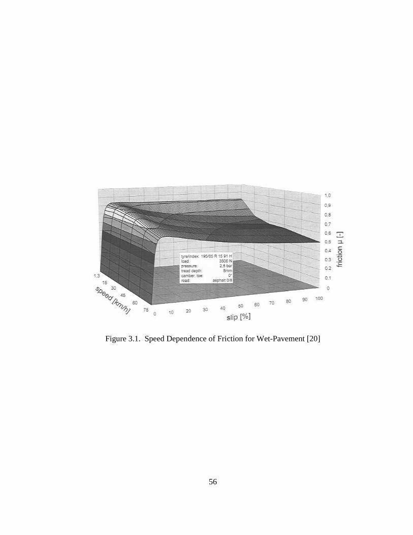
The approximation in (3.10), presented by J. Henry [6], has been found

elsewhere substantiating its validity. For example, T. Bachmann [20], provides a

graphical representation of (3.10) can be found and is presented below in Figure 3.1

for a particular tire on a wet road surface. The importance of (3.10) is significant

when coupled with the knowledge that the peak friction force typically occurs

between 10 and 20 % slip [11] for any given tire. In essence, a relative measure of

the peak friction force can be approximated for any given tire road combination with

the help of (3.10). With the ability to evaluate the friction force at low (between 10

and 20% slip) and full (100%) slip values for a given speed tire and road surface a

description of the characteristic brake force versus slip curve can be revealed [19].

The implication of this provides a basis for using two skid resistance tests conducted

at low and high vehicle speeds to classify and test a road surface with respect to a tire.

56

Figure 3.1. Speed Dependence of Friction for Wet-Pavement [20]

57

Expression (13), from Section 3.2.2, can be re-written to incorporate the

above assertion as,

FB[constant and negligible parameters] = fcn{SN low speed, SNhigh speed}, (3.11)

Expression (3.11) provides the construct—skid resistance testing, within which a

relative measure of the peak friction force and an exact measure of the skid friction

force may be tested and subsequently classified for a paved road surface with respect

to a particular tire. The vehicle speed, V, chosen for the SNhigh speed test, representing

the skid (sliding) friction force, is a free variable while the vehicle speed for the SNlow

speed test, representing the region of maximum attainable friction force, is constrained

by V and is estimated by equation (3.8). In essence, the road classification method is

providing the remaining two points, as the first is the origin or zero force zero slip

point, needed to estimate each of the three regions that make up the characteristic

brake force versus slip curve. The three regions are: the initial region characterized

by a positive linear slope beginning at the origin and ending slightly before the peak

friction value, the middle region characterized by negative quadratic slope (opening

downward) with the peak friction force value as its maximum point, and the final

region characterized by a negative linear slope converging to the skid friction force

value (see Section 2.3.3). Therefore the road classification method, encompassing

the two values represented by the skid tests at low and high vehicle speeds, together

with the zero slip zero force starting point determine the beginning, the middle and

the end of the characteristic brake force versus variable slip curve.

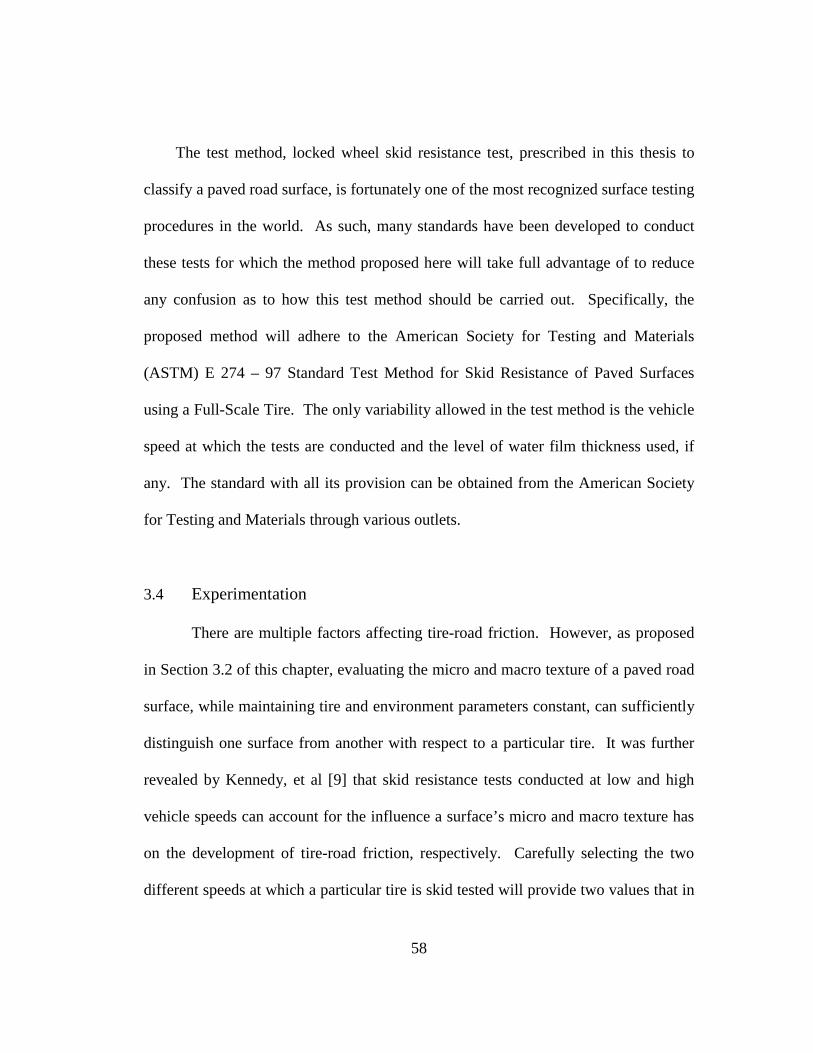
58

The test method, locked wheel skid resistance test, prescribed in this thesis to

classify a paved road surface, is fortunately one of the most recognized surface testing

procedures in the world. As such, many standards have been developed to conduct

these tests for which the method proposed here will take full advantage of to reduce

any confusion as to how this test method should be carried out. Specifically, the

proposed method will adhere to the American Society for Testing and Materials

(ASTM) E 274 – 97 Standard Test Method for Skid Resistance of Paved Surfaces

using a Full-Scale Tire. The only variability allowed in the test method is the vehicle

speed at which the tests are conducted and the level of water film thickness used, if

any. The standard with all its provision can be obtained from the American Society

for Testing and Materials through various outlets.

3.4 Experimentation

There are multiple factors affecting tire-road friction. However, as proposed

in Section 3.2 of this chapter, evaluating the micro and macro texture of a paved road

surface, while maintaining tire and environment parameters constant, can sufficiently

distinguish one surface from another with respect to a particular tire. It was further

revealed by Kennedy, et al [9] that skid resistance tests conducted at low and high

vehicle speeds can account for the influence a surface’s micro and macro texture has

on the development of tire-road friction, respectively. Carefully selecting the two

different speeds at which a particular tire is skid tested will provide two values that in

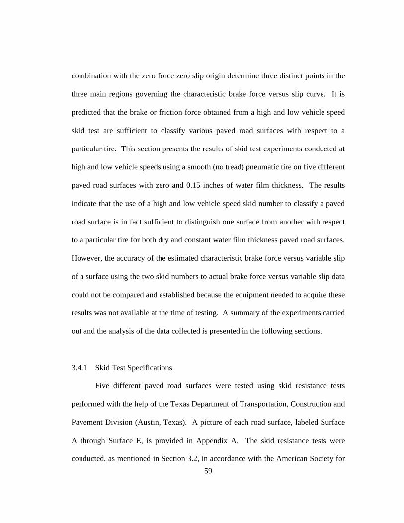
59

combination with the zero force zero slip origin determine three distinct points in the

three main regions governing the characteristic brake force versus slip curve. It is

predicted that the brake or friction force obtained from a high and low vehicle speed

skid test are sufficient to classify various paved road surfaces with respect to a

particular tire. This section presents the results of skid test experiments conducted at

high and low vehicle speeds using a smooth (no tread) pneumatic tire on five different

paved road surfaces with zero and 0.15 inches of water film thickness. The results

indicate that the use of a high and low vehicle speed skid number to classify a paved

road surface is in fact sufficient to distinguish one surface from another with respect

to a particular tire for both dry and constant water film thickness paved road surfaces.

However, the accuracy of the estimated characteristic brake force versus variable slip

of a surface using the two skid numbers to actual brake force versus variable slip data

could not be compared and established because the equipment needed to acquire these

results was not available at the time of testing. A summary of the experiments carried

out and the analysis of the data collected is presented in the following sections.

3.4.1 Skid Test Specifications

Five different paved road surfaces were tested using skid resistance tests

performed with the help of the Texas Department of Transportation, Construction and

Pavement Division (Austin, Texas). A picture of each road surface, labeled Surface

A through Surface E, is provided in Appendix A. The skid resistance tests were

conducted, as mentioned in Section 3.2, in accordance with the American Society for

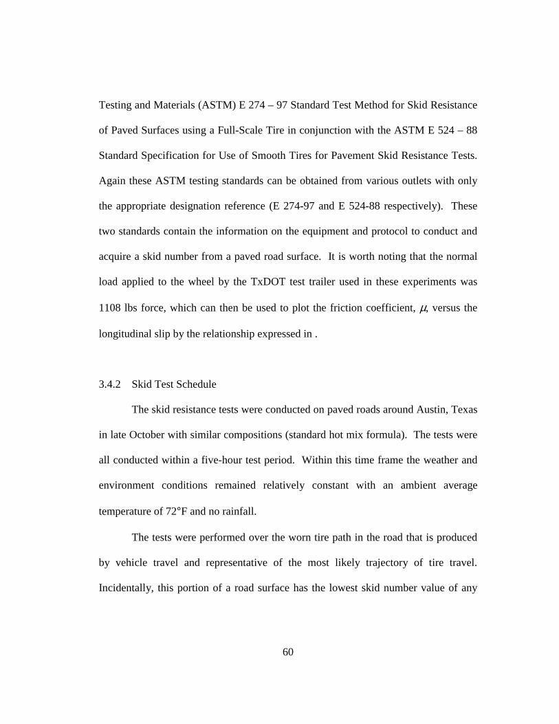
60

Testing and Materials (ASTM) E 274 – 97 Standard Test Method for Skid Resistance

of Paved Surfaces using a Full-Scale Tire in conjunction with the ASTM E 524 – 88

Standard Specification for Use of Smooth Tires for Pavement Skid Resistance Tests.

Again these ASTM testing standards can be obtained from various outlets with only

the appropriate designation reference (E 274-97 and E 524-88 respectively). These

two standards contain the information on the equipment and protocol to conduct and

acquire a skid number from a paved road surface. It is worth noting that the normal

load applied to the wheel by the TxDOT test trailer used in these experiments was

1108 lbs force, which can then be used to plot the friction coefficient, µ, versus the

longitudinal slip by the relationship expressed in .

3.4.2 Skid Test Schedule

The skid resistance tests were conducted on paved roads around Austin, Texas

in late October with similar compositions (standard hot mix formula). The tests were

all conducted within a five-hour test period. Within this time frame the weather and

environment conditions remained relatively constant with an ambient average

temperature of 72°F and no rainfall.

The tests were performed over the worn tire path in the road that is produced

by vehicle travel and representative of the most likely trajectory of tire travel.

Incidentally, this portion of a road surface has the lowest skid number value of any

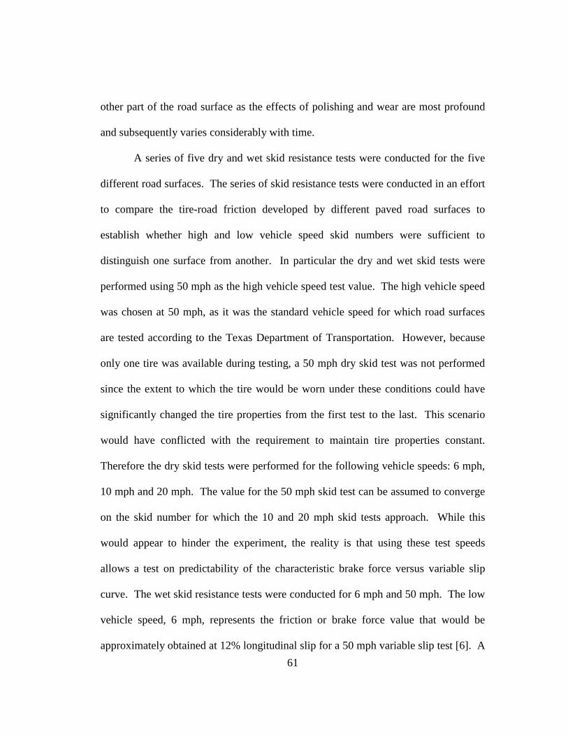
61

other part of the road surface as the effects of polishing and wear are most profound

and subsequently varies considerably with time.

A series of five dry and wet skid resistance tests were conducted for the five

different road surfaces. The series of skid resistance tests were conducted in an effort

to compare the tire-road friction developed by different paved road surfaces to

establish whether high and low vehicle speed skid numbers were sufficient to

distinguish one surface from another. In particular the dry and wet skid tests were

performed using 50 mph as the high vehicle speed test value. The high vehicle speed

was chosen at 50 mph, as it was the standard vehicle speed for which road surfaces

are tested according to the Texas Department of Transportation. However, because

only one tire was available during testing, a 50 mph dry skid test was not performed

since the extent to which the tire would be worn under these conditions could have

significantly changed the tire properties from the first test to the last. This scenario

would have conflicted with the requirement to maintain tire properties constant.

Therefore the dry skid tests were performed for the following vehicle speeds: 6 mph,

10 mph and 20 mph. The value for the 50 mph skid test can be assumed to converge

on the skid number for which the 10 and 20 mph skid tests approach. While this

would appear to hinder the experiment, the reality is that using these test speeds

allows a test on predictability of the characteristic brake force versus variable slip

curve. The wet skid resistance tests were conducted for 6 mph and 50 mph. The low

vehicle speed, 6 mph, represents the friction or brake force value that would be

approximately obtained at 12% longitudinal slip for a 50 mph variable slip test [6]. A

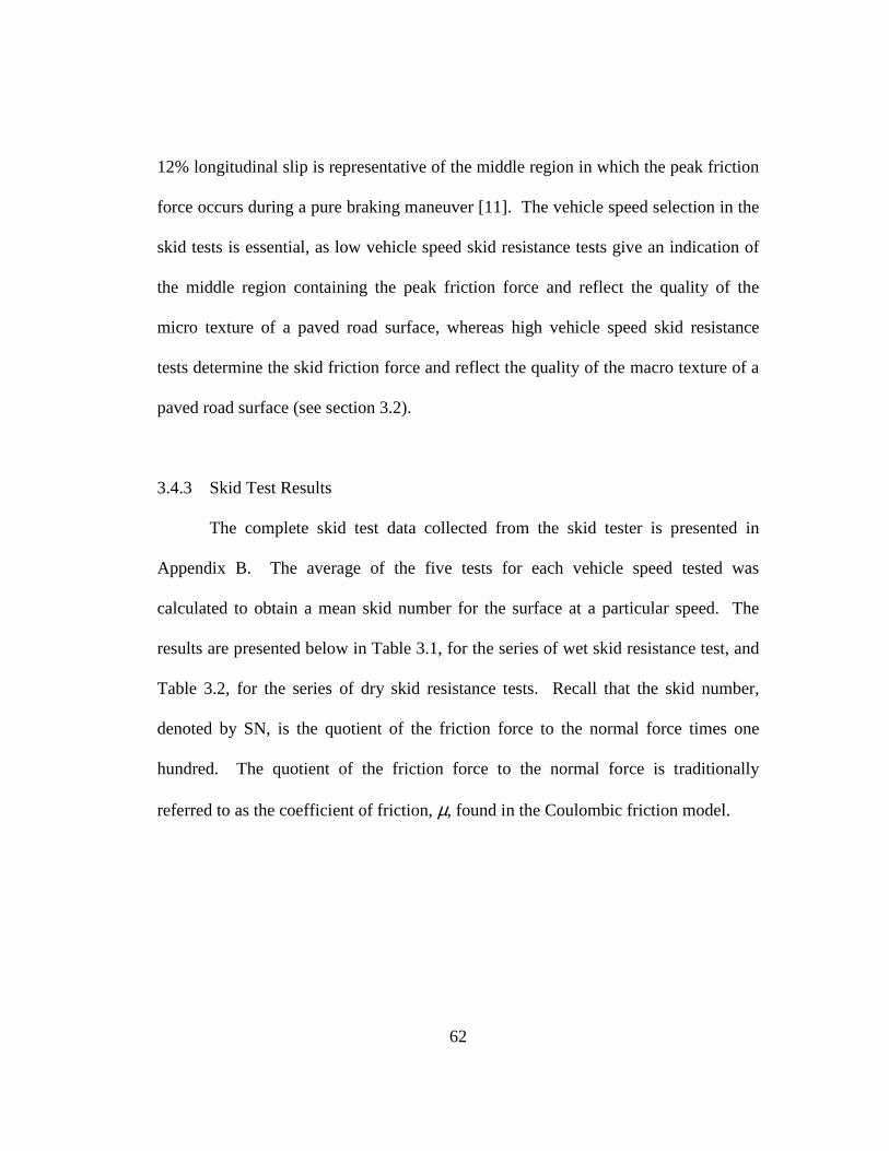
62

12% longitudinal slip is representative of the middle region in which the peak friction

force occurs during a pure braking maneuver [11]. The vehicle speed selection in the

skid tests is essential, as low vehicle speed skid resistance tests give an indication of

the middle region containing the peak friction force and reflect the quality of the

micro texture of a paved road surface, whereas high vehicle speed skid resistance

tests determine the skid friction force and reflect the quality of the macro texture of a

paved road surface (see section 3.2).

3.4.3 Skid Test Results

The complete skid test data collected from the skid tester is presented in

Appendix B. The average of the five tests for each vehicle speed tested was

calculated to obtain a mean skid number for the surface at a particular speed. The

results are presented below in Table 3.1, for the series of wet skid resistance test, and

Table 3.2, for the series of dry skid resistance tests. Recall that the skid number,

denoted by SN, is the quotient of the friction force to the normal force times one

hundred. The quotient of the friction force to the normal force is traditionally

referred to as the coefficient of friction, µ, found in the Coulombic friction model.

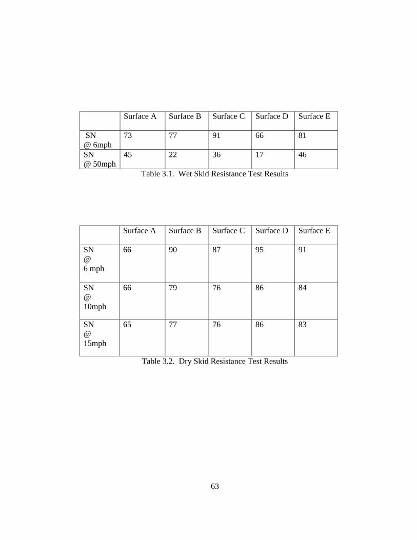
63

Surface A Surface B Surface C Surface D Surface E

SN @ 6mph

73 77 91 66 81

SN @ 50mph

45 22 36 17 46

Table 3.1. Wet Skid Resistance Test Results

Surface A Surface B Surface C Surface D Surface E

SN @ 6 mph

66

90 87 95 91

SN @ 10mph

66 79 76 86 84

SN @ 15mph

65 77 76 86 83

Table 3.2. Dry Skid Resistance Test Results

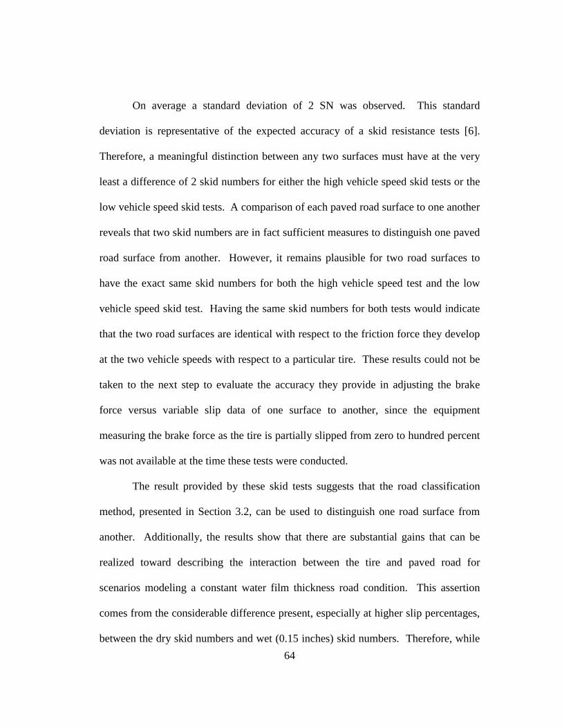
64

On average a standard deviation of 2 SN was observed. This standard

deviation is representative of the expected accuracy of a skid resistance tests [6].

Therefore, a meaningful distinction between any two surfaces must have at the very

least a difference of 2 skid numbers for either the high vehicle speed skid tests or the

low vehicle speed skid tests. A comparison of each paved road surface to one another

reveals that two skid numbers are in fact sufficient measures to distinguish one paved

road surface from another. However, it remains plausible for two road surfaces to

have the exact same skid numbers for both the high vehicle speed test and the low

vehicle speed skid test. Having the same skid numbers for both tests would indicate

that the two road surfaces are identical with respect to the friction force they develop

at the two vehicle speeds with respect to a particular tire. These results could not be

taken to the next step to evaluate the accuracy they provide in adjusting the brake

force versus variable slip data of one surface to another, since the equipment

measuring the brake force as the tire is partially slipped from zero to hundred percent

was not available at the time these tests were conducted.

The result provided by these skid tests suggests that the road classification

method, presented in Section 3.2, can be used to distinguish one road surface from

another. Additionally, the results show that there are substantial gains that can be

realized toward describing the interaction between the tire and paved road for

scenarios modeling a constant water film thickness road condition. This assertion

comes from the considerable difference present, especially at higher slip percentages,

between the dry skid numbers and wet (0.15 inches) skid numbers. Therefore, while

65

the experimentation with the road classification and test method was not fully realized

due to the absence of data relating the brake force exerted on the tire as the slip is

incrementally increased from zero to one hundred percent, the results indicate

favorably that road surfaces can be tested and subsequently categorized by those test

values (i.e. SN low speed, SNhigh speed) to distinguish one road surface from another. The

next chapter will discuss how the surface classification and test method, presented in

Section 3.2, can be used to adjust a specific empirical tire model called the Pacejka

Brake Tire Model.

66

CHAPTER 4: Integration of Road Classification and Test Method into the Pacejka Brake Tire Model

4.1 Introduction

The pneumatic tire is unique in that it is one of the only vehicle components

designed and manufactured independent of a specific vehicle design. As such, tire

manufacturers are obliged to provide a report, to vehicle manufacturers, quantifying a

tire’s performance capabilities [3]. This information is then assessed, in a vehicle

simulation, to identify the compatibility of a specific tire with a specific vehicle

model. However, in practice, the tire manufacturers often provide tire data measured

on laboratory test facilities whose frictional properties can be quite different from

actual road conditions. The use of this tire data can reduce the fidelity of vehicle

simulations [3]. An impasse is reached when one realizes that it would not be

feasible for a tire manufacture to measure, with a road tire test vehicle, every tire type

and size it produces on the many different proving grounds used by the various

vehicle manufacturers. Considerable attention by both vehicle and the tire

manufacturers has been given to rectifying this impasse. Specifically, Van der Jagt

and Parsons [3] looked into this problem and found that for a particular empirical tire

model, called the Pacejka Tire Model (see section 2.4.3), the adjustment of two

parameters sufficiently changes the tire model representing one surface to another

with respect to a particular tire. Withstanding its widespread use is the absence of a

standard method that can test and classify road surfaces so that the correction factors

67

themselves could be categorized and subsequently used to adjust the tire model for

any particular surface with respect to a particular tire. The construction of a road

surface classification method begs a subsequent question, namely if particular vehicle

types and thus particular tire types tend to be driven on particular road surfaces in the

United States. To address these issues the following sections present a review of a

method for correcting a Pacejka Tire model for a surface variation, the methodology

effecting a surface change in the Pacejka Brake Tire Model using the road

classification and test method, presented in Section 3.2, in conjunction with the

surface correction method developed by Van der Jagt and Parsons [3]. In addition the

last section of this chapter provides the results of a brief investigation into statistical

that relate current driving densities of particular vehicle types on particular roads in

the United States.

4.2 Review of Road Surface Correction in Pacejka Tire Model

The investigation by Van der Jagt and Parsons [3] isolated two parameters in

the Pacejka Tire Model sensitive to surface variation when testing a tire under a

cornering maneuver. The two parameters, D, the peak factor, and the product BCD,

associated with the tire stiffness, were found to transform a tire model representing

one surface to another by the linear approximations C1 and C2,

DActual Road = C1 (DTest Facility) and (4.1)

(BCD) Actual Road = C2 (BCDTest Facility). (4.2)

68

C1 and C2 represent the correction factors for a surface variation. To obtain these

correction factors two steps were taken. First, a full-scale force versus slip test of the

tire on an actual road surface was conducted. Second, the base or original Pacejka

Tire Model, developed on a test facility surface under a cornering maneuver, was

adjusted to approximate the recently conducted force versus slip data, developed from

the actual road surface. Specifically, by optimizing the two road correction factors C1

and C2 the error between the calculated tire model forces (derived from the test

facility surface) and the measured forces (derived from the full-scale test on an actual

road surface) was minimized. Figure 4.1 from Van der Jagt and Parsons [3]

illustrates the accuracy and predictability of using the BCD and D parameters to

adjust a tire model from one surface to another. More recently Domenichini, et al,

[19] investigated the applicability of the results established by Van der Jagt and

Parsons for the longitudinal case. Domenichini, et al, [19] found that the parameters

BCD and D could also be used to vary a road surface within the Pacejka Tire Model

when testing a tire under a pure braking action. They also established that a

minimum set of two experimental measures are required to represent the pavement

characteristic within the Pacejka Brake Tire Model. The development of the road

classification and test method, presented in Section 3.2, complement the preceding

argument made in [19].

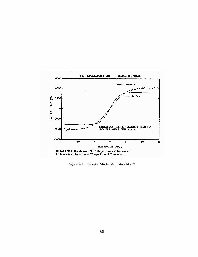
69

Figure 4.1. Pacejka Model Adjustability [3]

70

The proposed methodology by Van der Jagt and Parsons has a significant

shortcoming. Since the correction factors are for a particular surface they can only be

used for a limited time as the difference between the two surfaces is subject to change

according to weather, wear, and substantially different operating conditions. The

limited use of C1 and C2 to adjust a tire model from a reference surface to another can

be rectified if a standard is created to measure and test a road surface so that the

correction factors retain their meaning beyond a particular surface to a measure of a

surface that can be quantified at any time. By generalizing the condition of a road

surface to accommodate a classification and test method the correction factors can be

associated to a measurable characteristic of a road surface through a prescribed

classification criteria.

Van der Jagt and Parsons [3] identified that tire models based on data

measured on a surface other than the one on which the instrumented test was

performed can contribute to very large differences between simulation and

instrumented tire test results. This conclusion can be carried a step farther to say that

the difference between the brake force versus slip relationship from one surface to

another, whether going from a lab test surface to a real surface or from one real

surface to another, is significant enough to provide substantial gains in the fidelity of

vehicle simulations if corrected. The correction is accomplished by the manipulation

of two parameters sensitive to surface variation within the Pacejka Tire Model, BCD

and D [3]. This method should be valid for both the lateral and longitudinal force

71

case [19]. However, because there is no standard for which road surfaces can be

classified the use of these correction factors has a limited use. In response to this

shortcoming and with the claim made by Domenichini [19] that a minimum of two

experimental measurement are required, a basis for using the proposed road surface

classification and test method (see Section 3.2) to adjust a Pacejka Brake Tire Model

for a surface variation change is identified.

4.3 Integration

This section presents a methodology in which the road classification and test

method, presented in Section 3.2, can be used in conjunction with the method

formulated by Van der Jagt and Parsons [3] to effect a surface change in an empirical

tire model. However, before an explicit methodology is described, this section must

prove, if even for a fictitious road surface, that the Pacejka Brake Tire Model can be

adjusted using two values representative of the middle and final stage of the

characteristic brake force versus friction curve in accordance with the method

developed by Van der Jagt and Parsons [3].

4.3.1 Pacejka Brake Tire Model Adjustability Study

In order to proceed with a methodology effecting a surface change within the

Pacejka Brake Tire Model, it must be shown that the BCD and D parameters can be

scaled to adjust a tire model representing one surface to a new surface by using two

72

values classifying the new road surface coinciding with the friction force at low

(between 10 and 20%) and full (100%) slip percentages. Therefore this section

presents a case study conducted to evaluate whether the Pacejka Brake Tire Model

can be adjusted to go through the two arbitrary friction force values chosen at low and

full slip percentages. The case study was performed in Matlab using an actual

Pacejka Brake Tire Model developed by Pacejka, et al, [4] from tire measurements

taken on a dry asphalt road.

In order to substantiate the use of the correction methodology in conjunction

with the road classification method four scenarios must be validated. The friction

force values classifying a road surface in these scenarios were hypothetically

conceived and are not representative of actual skid test results. The first hypothetical

surface is one in which the friction force values at low and full slip percentages are

greater than their counterparts in the base Pacejka Brake Tire Model (F@ 10% slip =

6500 N, F@ 100% slip = 5000 N). The second hypothetical surface is the reverse case of

the first surface (F@ 10% slip = 5000 N, F@ 100% slip = 3800 N). The third hypothetical

surface is one in which the friction force value at the low slip percentage is greater

than its counterpart in the base Pacejka Tire Model whereas the friction force value at

the full slip percentage is less than its counterpart in the base Pacejka Brake Tire

Model (F@ 10% slip = 6500 N, F@ 100% slip = 4000 N). The fourth hypothetical surface is

the reverse case of the third surface (F@ 10% slip = 5500 N, F@ 100% slip = 5000 N).

Figures 4.2 and 4.3 show the results of this case study for the first and fourth surface

73

scenarios. The remaining two surface scenarios along with a representative Matlab

script used to generate the figures can be found in Appendix C.

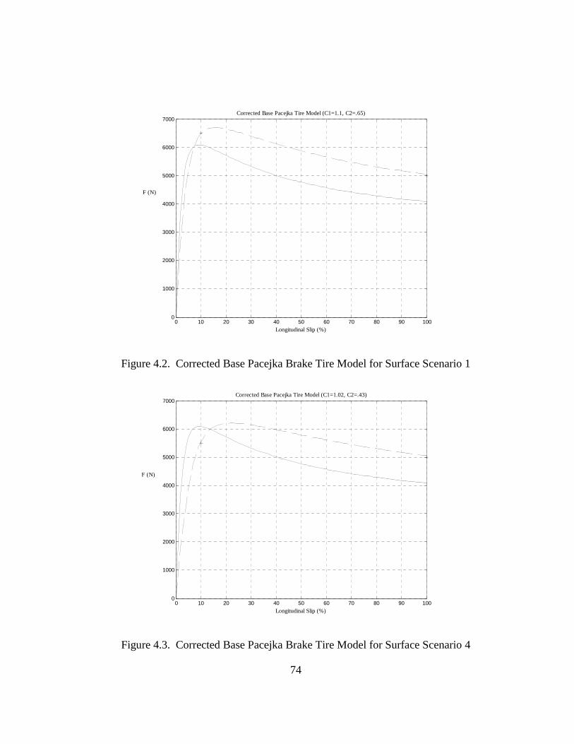
74

0 10 20 30 40 50 60 70 80 90 1000

1000

2000

3000

4000

5000

6000

7000

Longitudinal Slip (%)

Corrected Base Pacejka Tire Model (C1=1.1, C2=.65)

F (N)

Figure 4.2. Corrected Base Pacejka Brake Tire Model for Surface Scenario 1

0 10 20 30 40 50 60 70 80 90 1000

1000

2000

3000

4000

5000

6000

7000

Longitudinal Slip (%)

Corrected Base Pacejka Tire Model (C1=1.02, C2=.43)

F (N)

Figure 4.3. Corrected Base Pacejka Brake Tire Model for Surface Scenario 4

75

The results of this study indicate that the Pacejka Brake Tire Model can be

adjusted, using the BCD and D parameters, to two friction forces at low (between 10

and 20% slip) and full (100%) slip percentages, which can be obtained from two skid

tests at low and high vehicle speeds. It is foreseen that a computer program could

facilitate the calculation of the correction factors for a particular tire, independent of

running physical tests, as the correction based on two skid values is a determinant

system since skid numbers are integers ranging form 1 to 100 (i.e. all possibilities are

finite). Moreover it was inferred, from the above study, that the Pacejka Tire Model

might retain the information determining the slopes and inflection points of the three

regions making up the characteristic curve. Without the appropriate data to validate

this conjecture this thesis will assume that the adjusted tire model is actually a

representation of the new surface. However, the extent to which the correction

factors accurately predict a different road surface is unknown without performing a

comparison to the actual brake force versus variable slip data of a given surface. An

effort was made to perform a comparison study in the experimentation phase of the

road classification and test method, but it was not realized, as the appropriate testing

equipment to obtain brake force versus variable slip data was not available.

Consequently the comparison study is left to a subsequent investigation.

76

4.3.2 Assumptions and Constraints

A few assumptions are required in order to progress to a final methodology.

These assumptions are presented below.

• The use of the BCD and D parameters to adjust a base Pacejka Brake Tire

Model can be used to approximate any surface.

• The approximation of a new surface in a Pacejka Brake Tire Model, using the

two skid resistance values, is a sufficiently accurate prediction of the new

surface brake force versus variable slip behavior.

Along with the preceding assumptions, some constraints must be imposed on

the methodology varying the Pacejka Brake Tire Model for surface variations if using

the standard road classification and test method presented in Section 3.2 of this thesis.

These constraints are listed below.

• The locked wheel skid resistance test must follow ASTM standard E 274 - 97.

• The same tire (tread and compound) must be used to acquire the skid numbers

as was used to develop the base Pacejka Tire Model.

• The equivalent normal force must be used when adjusting the Pacejka Brake

Tire Model as was used when the skid numbers were acquired.

• The vehicle test speed used to obtain SNhigh speed must be equal to the vehicle

speed used to develop the base Pacejka Brake Tire Model. Consequently, the

second skid resistance test must be conducted at a low vehicle speed equal to

77

the product of the high vehicle speed and the percent slip where the maximum

friction force is obtained in the base Pacejka Brake Tire Model.

• For the case dealing with wet surfaces, both the base Pacejka Brake Tire

Model and the skid resistance tests must use the same Water Film Thickness.

(Note: the Pacejka Tire Model cannot predict the resulting force when water

depth is introduced or changed during testing. However, the Pacejka Tire

Model can model the behavior of the brake force versus variable slip if the

water film thickness is held constant throughout testing and hydroplaning does

not occur. This is a result based on the fact that the characteristic brake force

versus slip shape for a given water film thickness is retained although

categorically diminished (see Figure 2.7).)

• Knowledge of the environment conditions producing the skid resistance

values used to alter the base Pacejka Brake Tire Model should be reported, as

they inform on the relative conditions producing a given set of skid numbers.

4.3.3 Methodology

The premise of the methodology is that for a particular tire the appropriate

correction factors for adjusting a Pacejka Brake Tire Model from one surface to

another can be predicted with the help of a standard classification and test method.

The classification and test method classifies a paved road surface according to two

(locked-wheel) skid resistance tests taken at different vehicle speeds with a particular

78

tire. The (locked-wheel) skid resistance test for the high vehicle speed identifies the

friction force corresponding to the skid point or end point of the characteristic brake

force versus slip curve while the low vehicle speed identifies a friction force

corresponding to the peak friction region of the characteristic brake force versus slip

curve. The use of these two friction forces, estimated by skid values, in conjunction

with the zero force zero slip origin give a relative measure of how the characteristic

brake force versus slip curve should behave in the beginning, middle and end for a

particular tire and surface combination. The following describes a methodology to

effect a parametric surface change in the Pacejka Tire Model.

Part One

• Step One

A tire of interest is chosen.

• Step Two

A base Pacejka Brake Tire Model is developed from brake force versus

variable slip data for the tire chosen on a road surface.

• Step Three

A reference table with high and low skid numbers is constructed for the

particular tire chosen. An example table is presented below in Figure 4.4.

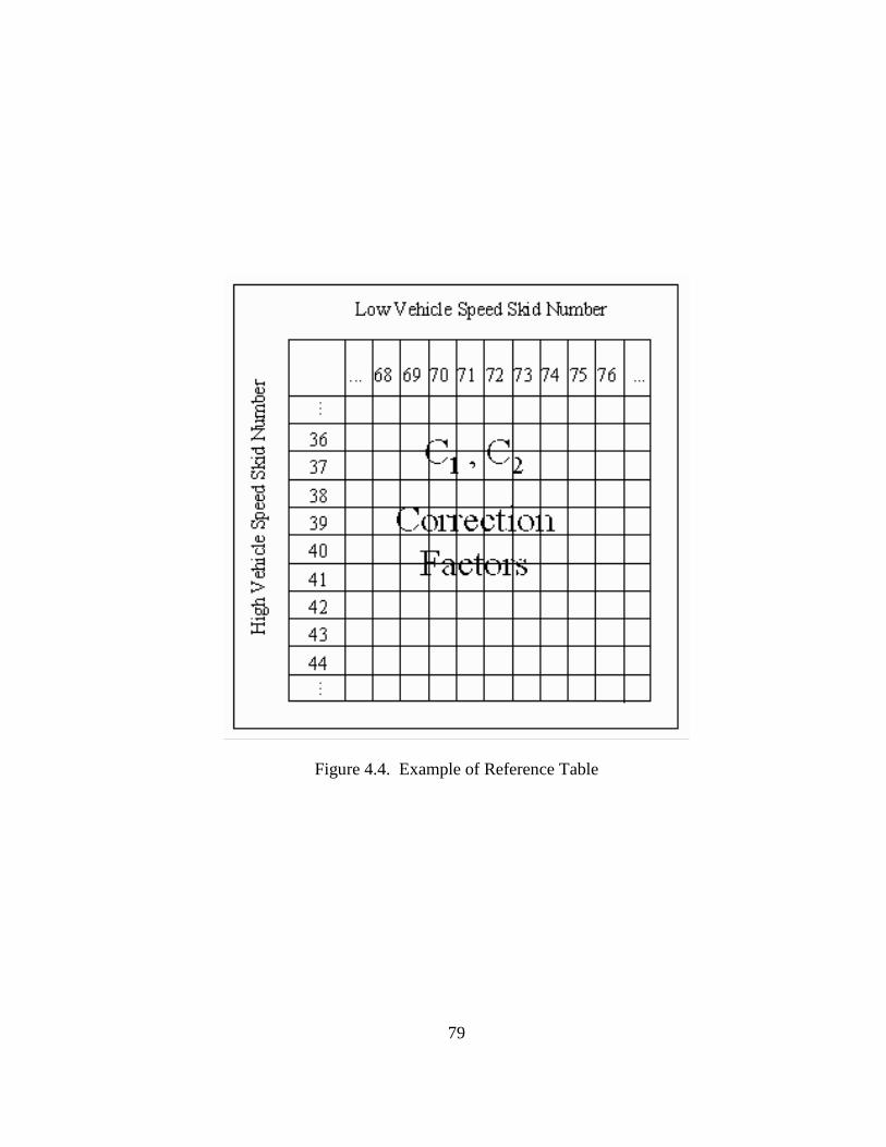
79

Figure 4.4. Example of Reference Table

80

Part Two

• Step One

A surface of interest is chosen.

• Step Two

The surface of interest is tested using two standard locked wheel skid

resistance test conducted at a high and a low vehicle speed (see Section 3.2).

• Step Three

The high and low vehicle speed skid numbers obtained from the test results

are used in conjunction with the reference table, obtained in Part One, Step

Three, to determine the correction factors needed to adjust the base Pacejka

Brake Tire Model to the new surface of interest.

The preceding methodology effecting a parametric surface change in the

Pacejka Brake Tire model has two important parts. The first part is a reference table

that contains the correction factors for any given combination of high and low vehicle

speed skid numbers with respect to a particular tire. This reference table identifies

the correction factors to the BCD and D parameters of the Pacejka Brake Tire Model

for any particular high and low skid number combination. Incidentally, the reference

table, in theory, would have 10,000 entries of correction factors for the different

combination resulting from a 100 by 100 array of skid numbers (skid numbers range

from 1 to 100). However, the capability and accuracy of C1 and C2 to describe all of

these scenarios is highly questionable. It would be useful to have knowledge of the

81

road surfaces a specific vehicle type is likely to traverse so as to provide a relevant

range of skid numbers in the reference table. To address this specific issue, Section

4.4 describes statistical studies furnished by the Federal Highway Administration on

driving density in the United States. It is left to a subsequent investigation to

determine the extent to which the correction factors can accurately predict a surface

change.

The second part is the testing of a paved road surface to identify its high and

low vehicle speed skid number with respect to the same tire. It is important that the

vehicle speed, V, normal force, FNormal, and water film thickness, t, if any used to

determine the base Pacejka Tire Model are also used when classifying and testing a

paved road surface with respect to a particular tire. Additionally the low slip number,

which is established to correspond with the low vehicle speed skid test, must be

consistently maintained for each surface tested with respect to a particular tire. The

choice of the low slip value, and consequently the low vehicle speed, can be

anywhere from 10 to 20% [11], with 15% being a good representation of the peak

friction force region of the characteristic brake force versus slip curve. See equation

(3.8) for the formula approximating the friction force using a low vehicle speed skid

test. Together these two pieces of information allow a base Pacejka Tire Model to be

adjusted to represent any paved road surface. It is important to stress that the

reference table, the testing method, and the base Pacejka Brake Tire Model must be

developed and performed with respect to the same tire, normal force, vehicle speeds

and water film thickness.

82

4.4 Driving Densities in the United States

In general knowledge of the road surface a specific vehicle type will traverse

allows engineers developing vehicle simulations the ability to improve the tire models

that describe the interaction between the tire and road surface in an effort to better

assess the actual response of a vehicle in a particular environment. However, in order

to use this knowledge of vehicle driving densities in a vehicle simulation, a

methodology to test, classify, and adjust tire models according to different road

surfaces must be available. Section 4.3 presents such a methodology. In order to

determine these driving densities it was hypothesized that the statistical studies

published by the Federal Highway Administration (FHWA) and the Bureau of

Transportation Statistics were capable of relating the relevant road surfaces a

particular vehicle type is likely to drive on during normal use. It is the purpose of this

section to present the available information useful in identifying the road surfaces

vehicle types are likely to drive on and the extent to which this information can be

used to relate the trends for specific vehicle types. It was determined that, as of the

most recent FHWA study, only the number of miles traveled on specific functional

roadway systems by a particular vehicle type can be related. Further information

regarding the composition of roadways exists, but this information cannot be

connected to the driving trends of a particular vehicle type. A future statistic relating

the vehicle types traversing the different road surface types among the different

83

functional roadway systems across the United States is determined necessary to give

relevance to the road surface a specific vehicle type will traverse.

4.4.1 Highway Statistics Background

Highway statistics come from various administrative agencies within the 50

states, over 30,000 units of local government, Federal agencies, and the five U.S.

territories [21]. The Office of Highway Policy Information publishes the findings in

Highway Statistics. The statistical studies are provided by the FHWA under a

directive by Congress to aid in highway planning, programming, budgeting

forecasting, and fiscal management. The information presented in Highway Statistics

“meets the Federal need of providing a national perspective on highway program

activities” [21]. The statistical information, presented in this section, is based on the

Highway Statistic report for the year 1999.

4.4.2 Vehicle Type Classification

The specific vehicle types identified by the statistical studies are classified

into passenger cars, motorcycles, other 2-axle 4-tire vehicles, buses, single-unit 2-axel

6-tire or more trucks, and combination trucks. The number of current vehicle

registrations from each of the fifty states accounts for the number of vehicles in the

study. Of particular note is the grouping of other 2-axle 4-tire vehicles, which

includes vans, pick-up trucks, and sport-utility vehicles.

84

4.4.3 Functional Roadway Systems

The functional roadway systems contain rural and urban stratifications. This

initial distinction is determined by the number of persons per square mile that

encompass at a minimum the land area delineated by the results from the last U.S.

census. The cut-off of inhabitants distinguishing an urbanized area from a rural one

is a population of 50,000 people. Within these two areas, urban and rural, is a

functional grouping or system of public roads according to the character of service

the roads are intended to provide. The functional systems are: (1) arterial highways,

which handle long distance travel; (2) collector facilities, which collect and disperse

traffic between the arterials and the lower level roads; and (3) local roads, streets, and

other public ways, which serve a land access function to homes, businesses,

individual farms and ranches, and other uses [21].

4.4.4 Road Surface Classification

The road surfaces identified by these statistical studies are classified according

to their composition. The classification of road surfaces exists within the different

functional roadway systems. Figure 4.5 provides a visual description of the following

stratification of road surfaces. Paved and unpaved road surfaces represent the first

stratum, with unpaved roads having no other substrata. Under paved roads, the

second stratum classifies paved roads as low, intermediate and high type. A low type

paved surface is defined as an earth, gravel, or stone roadway having a bituminous (a

black, tarry mineral substance used in cements and in the construction of pavement)

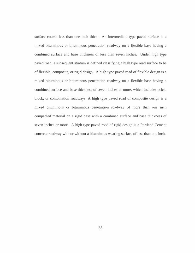
85

surface course less than one inch thick. An intermediate type paved surface is a

mixed bituminous or bituminous penetration roadway on a flexible base having a

combined surface and base thickness of less than seven inches. Under high type

paved road, a subsequent stratum is defined classifying a high type road surface to be

of flexible, composite, or rigid design. A high type paved road of flexible design is a

mixed bituminous or bituminous penetration roadway on a flexible base having a

combined surface and base thickness of seven inches or more, which includes brick,

block, or combination roadways. A high type paved road of composite design is a

mixed bituminous or bituminous penetration roadway of more than one inch

compacted material on a rigid base with a combined surface and base thickness of

seven inches or more. A high type paved road of rigid design is a Portland Cement

concrete roadway with or without a bituminous wearing surface of less than one inch.

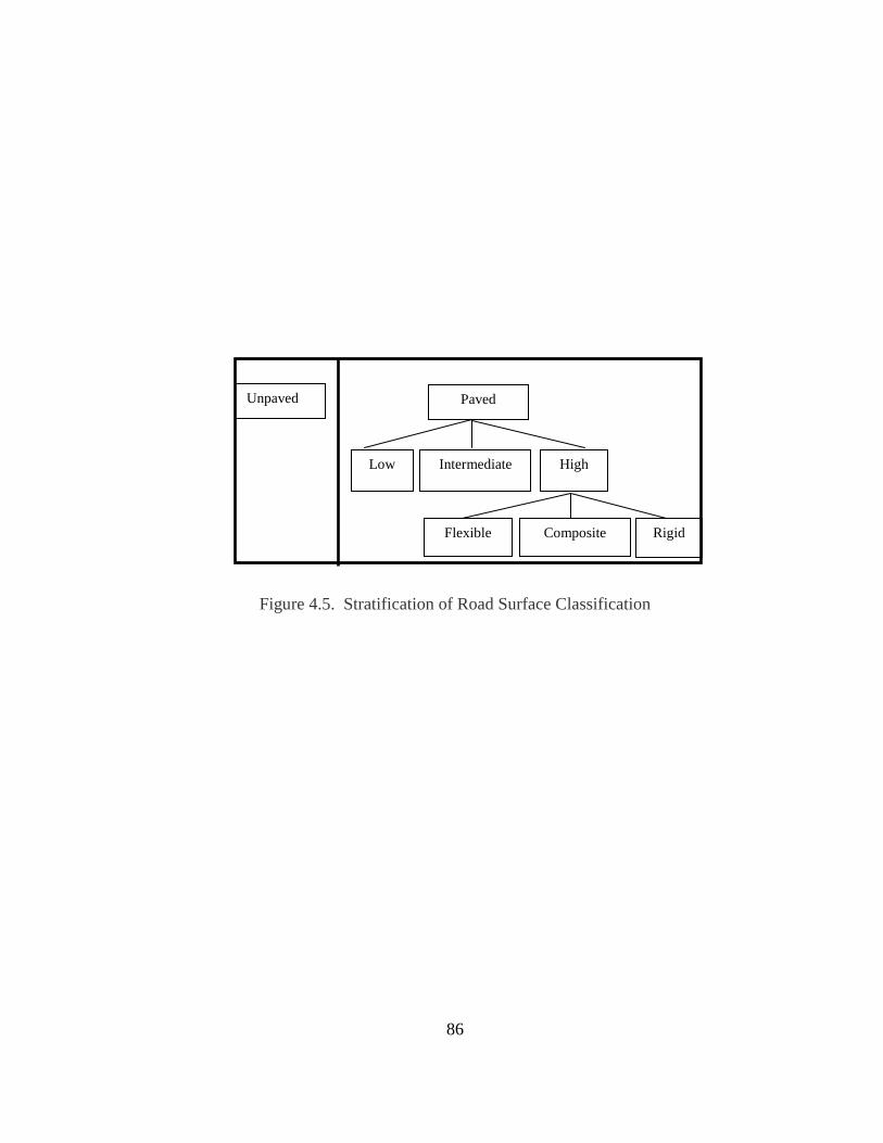
86

Figure 4.5. Stratification of Road Surface Classification

Unpaved Paved

High Intermediate

Rigid Composite Flexible

Low

87

4.4.5 Relevant Statistical Studies and Analysis

The purpose of researching these statistical studies is to determine whether

vehicle designers can be informed of the likely road surface a specific vehicle type

will traverse. With this in mind, a search of relevant statistical studies presented in

the 1999 Highway Statistics Report was undertaken. Three studies were identified,

and can be found in their entirety in [21], as potentially useful: (1) State Motor-

Vehicle Registrations-1999 1/ [21], which relates the number of motor vehicles and

the distribution of those vehicles into the specific types of vehicles for each state; (2)

Annual Vehicle Distance Traveled in Miles and Related Data – 1999 1/ By Highway

Category and Vehicle Type [21], which relates the number of miles traveled by

specific vehicle types over specific functional roadway systems; (3) Public Road

Length– 1999 1/ Miles by Type of Surface and Ownership/ Functional System

National Summary [21], which relates the length, measured in miles, of a particular

road surface type present in the different functional roadway systems.

The first statistical study, State Motor-Vehicle Registrations-1999 1/ [21],

gives the most accurate account of the number of vehicles on roadways today. This

statistical study also has the potential to describe a regional demographic of vehicle

use and potentially inform on how to better design for local environment use by

measure of the density of specific vehicle types in certain regional areas. Figure 4.6

displays a comparison of the number of automobiles to the number of trucks in from a

sample of U.S. States. The information plotted comes directly from the statistical

study without manipulation. The inferred use of this study is to use the number of

88

registered vehicles in use in a particular state to obtain the total national miles

traveled on functional roadway systems in the United States by specific vehicle types

from the average number of miles driven by a specific vehicle type on a functional

roadway system in a particular state.

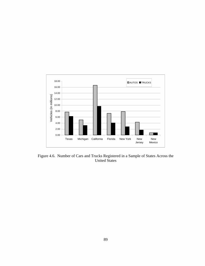
89

0.00

2.00

4.00

6.00

8.00

10.00

12.00

14.00

16.00

18.00

Texas Michigan California Florida New York NewJersey

NewMexico

Veh

icle

s (in

mill

ions

)

AUTOS TRUCKS

Figure 4.6. Number of Cars and Trucks Registered in a Sample of States Across the United States

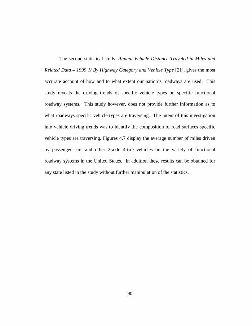
90

The second statistical study, Annual Vehicle Distance Traveled in Miles and

Related Data – 1999 1/ By Highway Category and Vehicle Type [21], gives the most

accurate account of how and to what extent our nation’s roadways are used. This

study reveals the driving trends of specific vehicle types on specific functional

roadway systems. This study however, does not provide further information as to

what roadways specific vehicle types are traversing. The intent of this investigation

into vehicle driving trends was to identify the composition of road surfaces specific

vehicle types are traversing. Figures 4.7 display the average number of miles driven

by passenger cars and other 2-axle 4-tire vehicles on the variety of functional

roadway systems in the United States. In addition these results can be obtained for

any state listed in the study without further manipulation of the statistics.

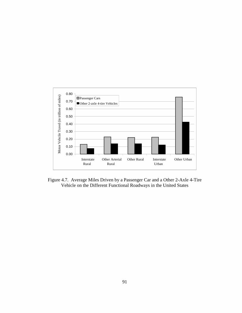
91

0.00

0.10

0.20

0.30

0.40

0.50

0.60

0.70

0.80

InterstateRural

Other ArterialRural

Other Rural InterstateUrban

Other Urban

Mot

or V

ehci

le T

rave

l (in

trill

ion

of m

iles)

Passenger Cars

Other 2-axle 4-tire Vehicles

Figure 4.7. Average Miles Driven by a Passenger Car and a Other 2-Axle 4-Tire Vehicle on the Different Functional Roadways in the United States

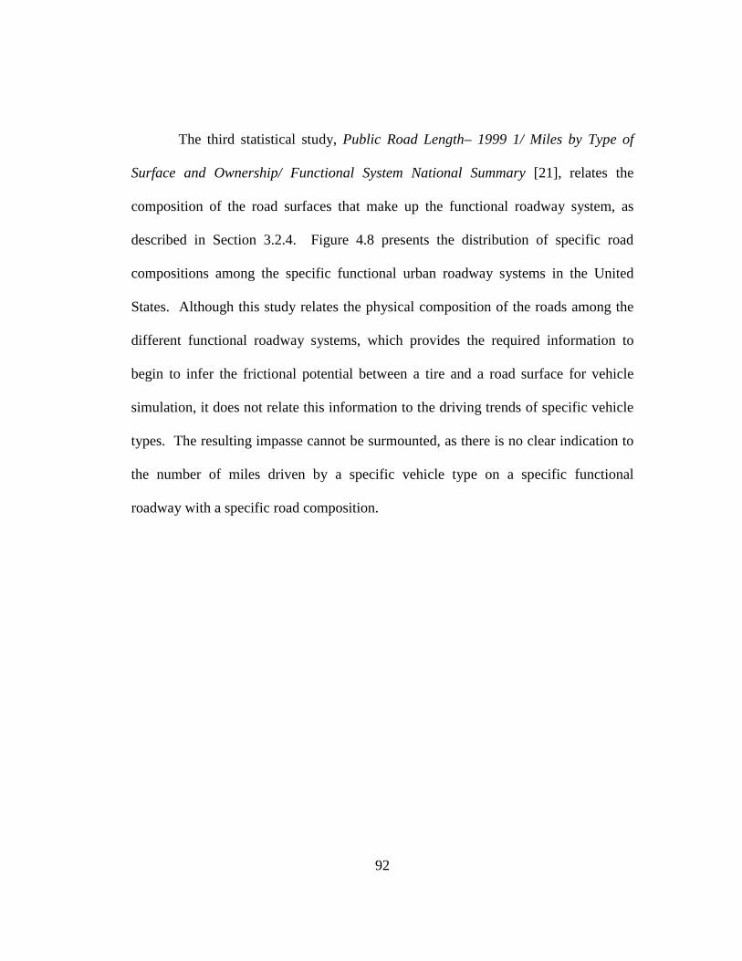
92

The third statistical study, Public Road Length– 1999 1/ Miles by Type of

Surface and Ownership/ Functional System National Summary [21], relates the

composition of the road surfaces that make up the functional roadway system, as

described in Section 3.2.4. Figure 4.8 presents the distribution of specific road

compositions among the specific functional urban roadway systems in the United

States. Although this study relates the physical composition of the roads among the

different functional roadway systems, which provides the required information to

begin to infer the frictional potential between a tire and a road surface for vehicle

simulation, it does not relate this information to the driving trends of specific vehicle

types. The resulting impasse cannot be surmounted, as there is no clear indication to

the number of miles driven by a specific vehicle type on a specific functional

roadway with a specific road composition.

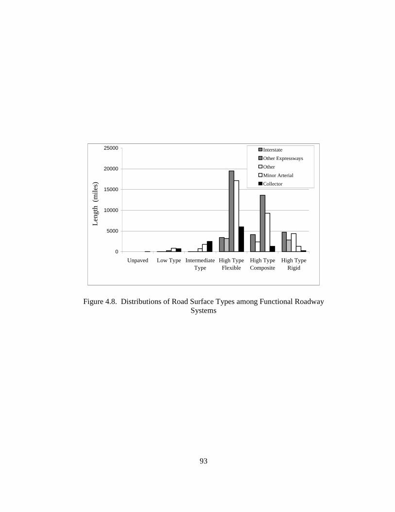
93

0

5000

10000

15000

20000

25000

Unpaved Low Type IntermediateType

High TypeFlexible

High TypeComposite

High TypeRigid

Len

gth

(m

iles)

Interstate

Other Expressways

Other

Minor Arterial

Collector

Figure 4.8. Distributions of Road Surface Types among Functional Roadway Systems

94

While this investigation into the statistical breakdown of public road use did

not produce the intended statistic—the number of miles traveled by a specific vehicle

type on a specific functional roadway composed of a specific road type; this study did

account for the number of specific vehicle types in use in each of the fifty states in the

United States, the number of miles traveled by specific vehicle types on specific

functional roadway systems and a system stratifying the composition of road surfaces

among the different functional roadway systems. Unfortunately, without the intended

statistic, an assessment of the relevant range of road surfaces a specific vehicle

simulation should consider when using the methodology effecting a parametric

surface change in the Pacejka Tire Model, presented in Section 4.3, could not be

established. The prospect that the required statistic will be made available in the near

future is not unlikely, as there is already a way to account for the number of vehicles

traversing a known roadway type and there is also a way of differentiating the

different road compositions present among the different functional roadway systems.

However, in order to see the fruition of this statistic, road makers and local

governments must be made aware of the potential safety benefits resulting from such

a statistic.

95

CHAPTER 5: Recommendation for Future Work and Conclusion

5.1 Paved Road Classification and Test Method

The objective for this thesis has been met. A paved road classification and

test method identifying the dominant surface characteristics contributing to the

development of friction with respect to a pneumatic tire was developed. This method

classifies and tests paved road surfaces using a high and low vehicle speed skid test.

The potential of this thesis to be of relevant use to vehicle, tire and road makers will

be realized when the technologies facilitating the acquisition of skid numbers from

optical measurements comes to fruition. A methodology effecting a parameter

surface change in the Pacejka Brake Tire Model is proposed. This methodology

combines the classification and test method developed in this thesis with a surface

correction method to the Pacejka Tire Model, developed by [3]. It is forecasted that

vehicle makers could use such a methodology to improve and tune specific

component designs within a specific vehicle design that are influenced by the tire-

road interaction. While road makers could use this methodology in conjunction with

vehicle simulations to test surfaces against a standard tire in order to determine safe

driving conditions and or evaluate the quality of a road surface.

96

5.2 Future Work

There is considerable work left before this paved road classification and test

method can be fully implemented. First and foremost the application of the

classification and test method used to approximate another surface in the Pacejka Tire

Model must be checked and its accuracy to actual tire test data must be established.

Once this classification and test method has been verified, research into the use of

different tires may be pursued as well as extending the methodology to the cornering

or lateral force case. This section briefly goes over the aforementioned future work.

5.2.1 Verification of Proposed Methodology

It is imperative that the conjectures and assumption asserted in this thesis be

verified. In particular are the two assumptions needed to apply the paved road

classification and test method to effect a parameter surface change in the Pacejka

Brake Tire Model. First the extent to which the correction method can be used to

approximate a new surface must be examined. Next the approximation of a new

surface in a Pacejka Brake Tire Model, using the classification and test method, must

be compared to actual brake force versus variable slip tire data to determine the

accuracy and range of adaptability of a new surface.

97

5.2.2 Evaluating Other Tire Types

The development of this thesis based its conclusions by maintaining the same

tire type and properties. The paved road and classification method is thus developed

to represent the behavior of a specific tire with respect to a specific surface.

However, if this classification and test method is to have any widespread success it

must be developed to account for tires with variable tread depth and patterns.

5.2.3 Extending Classification and Test Method to Lateral Force Case

The development of this thesis was based on a pure braking vehicle action.

However, many vehicle situations call for both pure braking and cornering analysis.

As such it would be of interest to investigate the adaptability of this classification and

test method to the lateral force case. To this end there exist side force skid testing

methods and testing equipment already in use by various departments of

transportation.

5.3 Conclusion

The classification and test method developed in this thesis can facilitate the

adjustment of the Pacejka Tire Model due to a surface variation when combined with

the tire data correction method developed by Van der Jagt and Parsons [3]. This

approach requires as much full-scale testing as is currently needed to generate a new

Pacejka Tire Model on a given surface, and it still requires verification. However,

98

this may change as new technologies will facilitate the acquisition of skid numbers

from optical measurements. In this way, the classification and test method

formulated here represents advancement in the tools available to vehicle and road

makers to improve predictability of tire forces over different surfaces. In this way,

the safety of vehicles on roadways and an understanding of how the two are

interrelated can be gained.

99

Appendix A: Images of Tested Road Surfaces

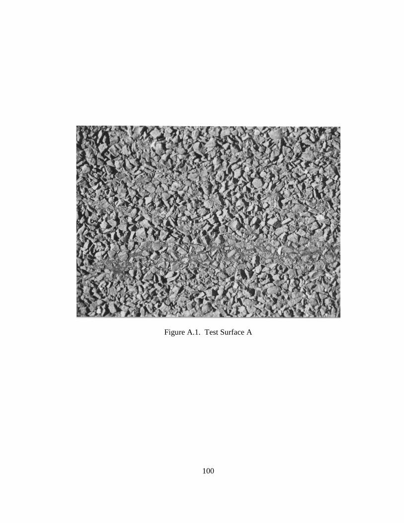
100

Figure A.1. Test Surface A

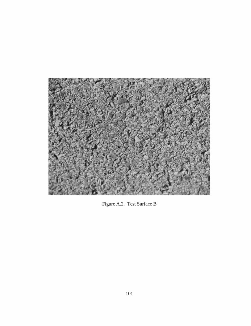
101

Figure A.2. Test Surface B

102

Figure A.3. Test Surface C

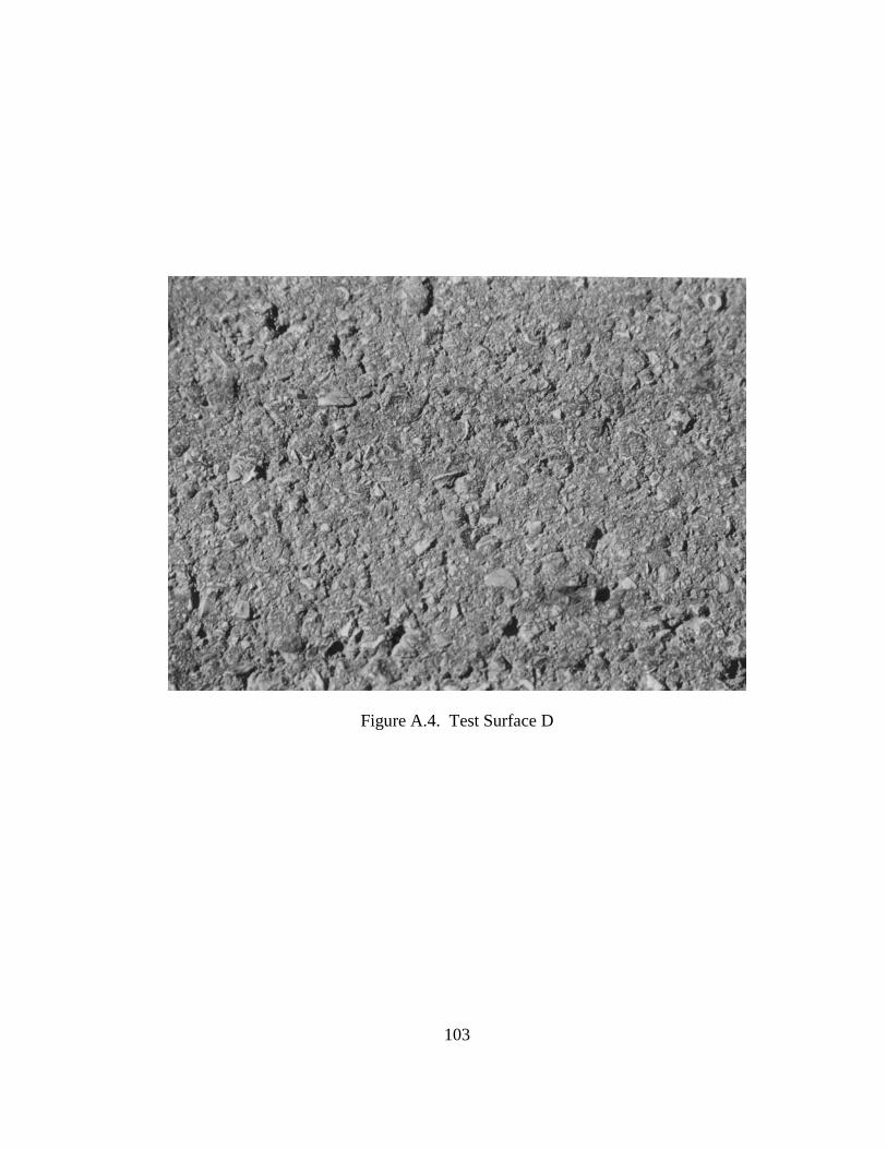
103

Figure A.4. Test Surface D

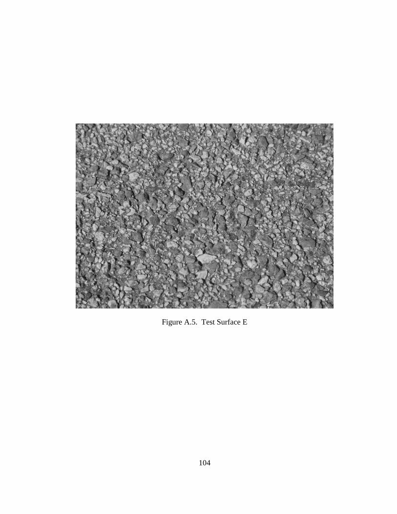
104

Figure A.5. Test Surface E

105

Appendix B: Skid Test Data

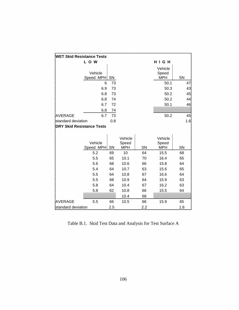
106

WET Skid Resistance Tests L O W H I G H

Vehicle

Speed MPH SN

Vehicle Speed MPH SN

6 73 50.1 47 6.9 73 50.3 43 6.8 73 50.2 45 6.8 74 50.2 44 6.7 72 50.1 46

6.8 74 AVERAGE 6.7 73 50.2 45 standard deviation 0.8 1.6 DRY Skid Resistance Tests

Vehicle

Speed MPH SN

Vehicle Speed MPH SN

Vehicle Speed MPH SN

5.2 69 10 64 15.5 68 5.5 65 10.1 70 16.4 65 5.6 68 10.6 66 15.8 64 5.4 64 10.7 63 15.6 65 5.5 64 10.8 67 16.6 64 5.5 68 10.9 64 15.9 63 5.8 64 10.4 67 16.2 63 5.8 62 10.8 66 15.5 64

10.4 68 AVERAGE 5.5 66 10.5 66 15.9 65 standard deviation 2.5 2.2 1.6

Table B.1. Skid Test Data and Analysis for Test Surface A

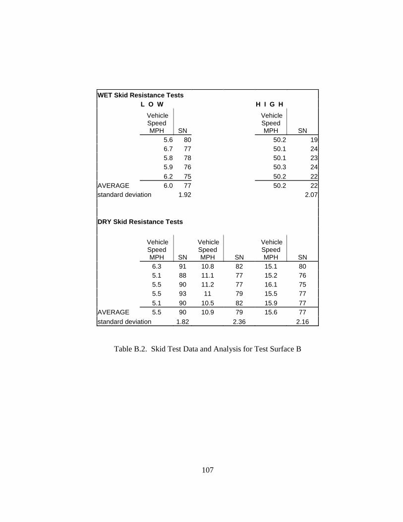
107

WET Skid Resistance Tests L O W H I G H

Vehicle Speed MPH SN

Vehicle Speed MPH SN

5.6 80 50.2 19 6.7 77 50.1 24 5.8 78 50.1 23 5.9 76 50.3 24

6.2 75 50.2 22 AVERAGE 6.0 77 50.2 22 standard deviation 1.92 2.07 DRY Skid Resistance Tests

Vehicle Speed MPH SN

Vehicle Speed MPH SN

Vehicle Speed MPH SN

6.3 91 10.8 82 15.1 80 5.1 88 11.1 77 15.2 76 5.5 90 11.2 77 16.1 75 5.5 93 11 79 15.5 77

5.1 90 10.5 82 15.9 77 AVERAGE 5.5 90 10.9 79 15.6 77

standard deviation 1.82 2.36 2.16

Table B.2. Skid Test Data and Analysis for Test Surface B

108

WET Skid Resistance Tests L O W H I G H

Vehicle Speed MPH SN

Vehicle Speed MPH SN

5.5 89 50.6 35 5.4 91 50.4 37 5.5 92 50.4 35

7.2 90 50.8 32 AVERAGE 5.9 91 50.5 35 standard deviation 1.29 2.06 DRY Skid Resistance Tests

Vehicle Speed MPH SN

Vehicle Speed MPH SN

Vehicle Speed MPH SN

5.9 89 10.4 78 15.1 76 5.9 88 11.2 75 15.6 78 6.6 88 10.7 76 15.9 75 5.8 85 10.3 78 15.6 78

6.1 86 10.5 75 15.2 75 AVERAGE 6.1 87 10.6 76 15.5 76

standard deviation 1.64 1.52 1.52

Table B.3. Skid Test Data and Analysis for Test Surface C

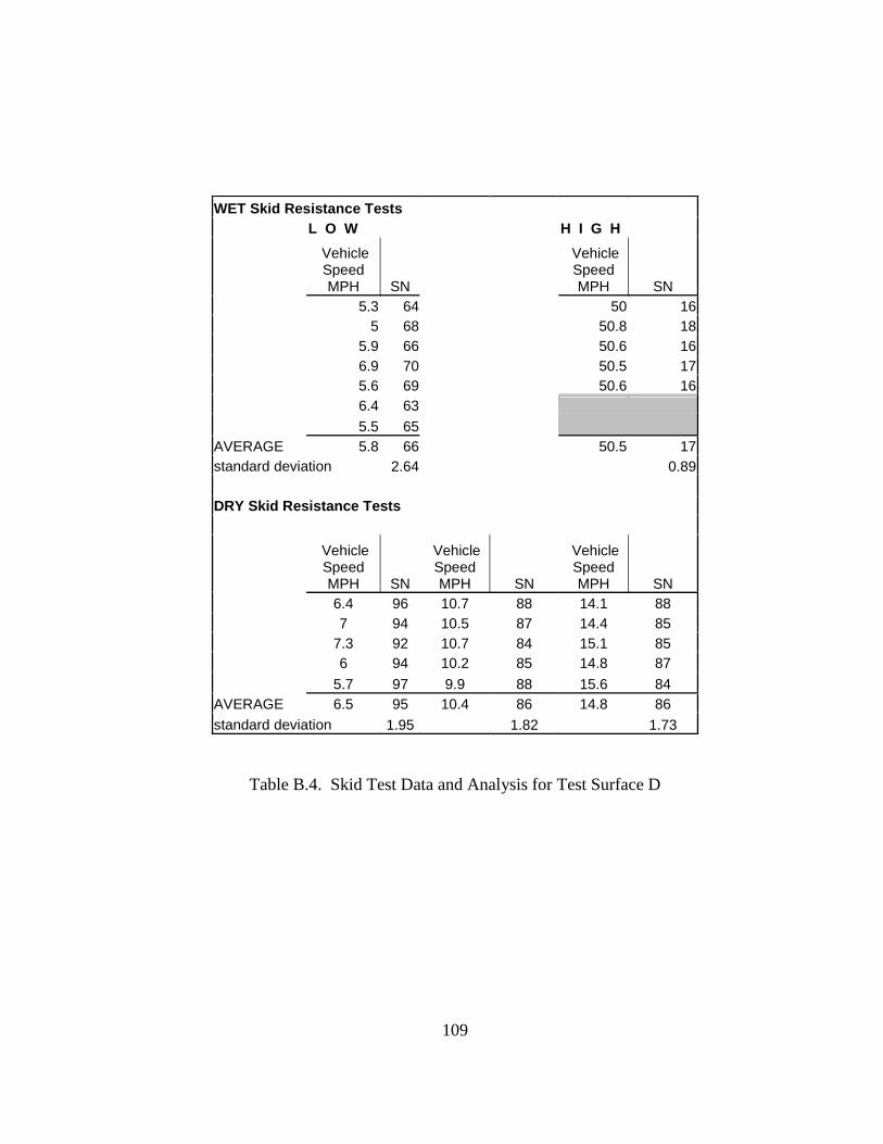
109

WET Skid Resistance Tests L O W H I G H

Vehicle Speed MPH SN

Vehicle Speed MPH SN

5.3 64 50 16 5 68 50.8 18 5.9 66 50.6 16 6.9 70 50.5 17 5.6 69 50.6 16 6.4 63

5.5 65 AVERAGE 5.8 66 50.5 17 standard deviation 2.64 0.89 DRY Skid Resistance Tests

Vehicle Speed MPH SN

Vehicle Speed MPH SN

Vehicle Speed MPH SN

6.4 96 10.7 88 14.1 88 7 94 10.5 87 14.4 85 7.3 92 10.7 84 15.1 85 6 94 10.2 85 14.8 87

5.7 97 9.9 88 15.6 84 AVERAGE 6.5 95 10.4 86 14.8 86 standard deviation 1.95 1.82 1.73

Table B.4. Skid Test Data and Analysis for Test Surface D

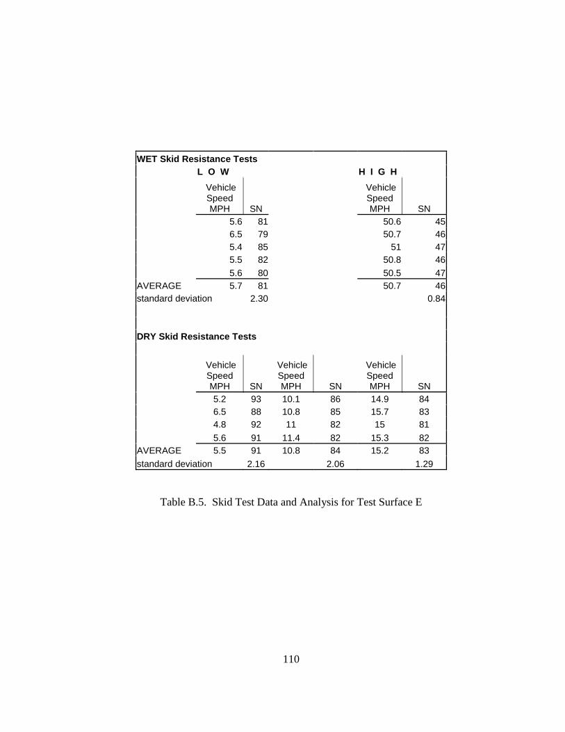
110

WET Skid Resistance Tests L O W H I G H

Vehicle Speed MPH SN

Vehicle Speed MPH SN

5.6 81 50.6 45 6.5 79 50.7 46 5.4 85 51 47 5.5 82 50.8 46

5.6 80 50.5 47 AVERAGE 5.7 81 50.7 46 standard deviation 2.30 0.84 DRY Skid Resistance Tests

Vehicle Speed MPH SN

Vehicle Speed MPH SN

Vehicle Speed MPH SN

5.2 93 10.1 86 14.9 84 6.5 88 10.8 85 15.7 83 4.8 92 11 82 15 81

5.6 91 11.4 82 15.3 82 AVERAGE 5.5 91 10.8 84 15.2 83

standard deviation 2.16 2.06 1.29

Table B.5. Skid Test Data and Analysis for Test Surface E

111

Appendix C: Pacejka Brake Tire Model Adjustability Study

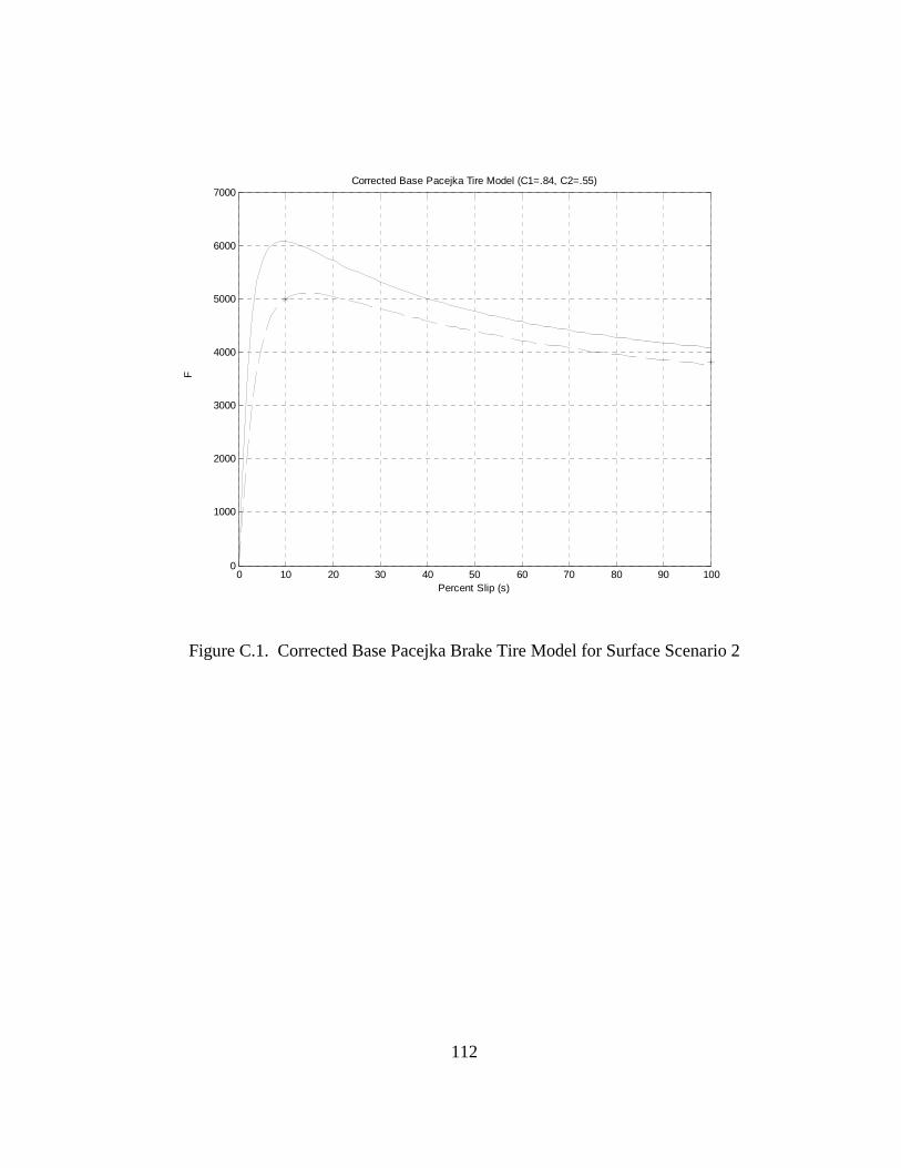
112

0 10 20 30 40 50 60 70 80 90 1000

1000

2000

3000

4000

5000

6000

7000

Percent Slip (s)

FCorrected Base Pacejka Tire Model (C1=.84, C2=.55)

Figure C.1. Corrected Base Pacejka Brake Tire Model for Surface Scenario 2

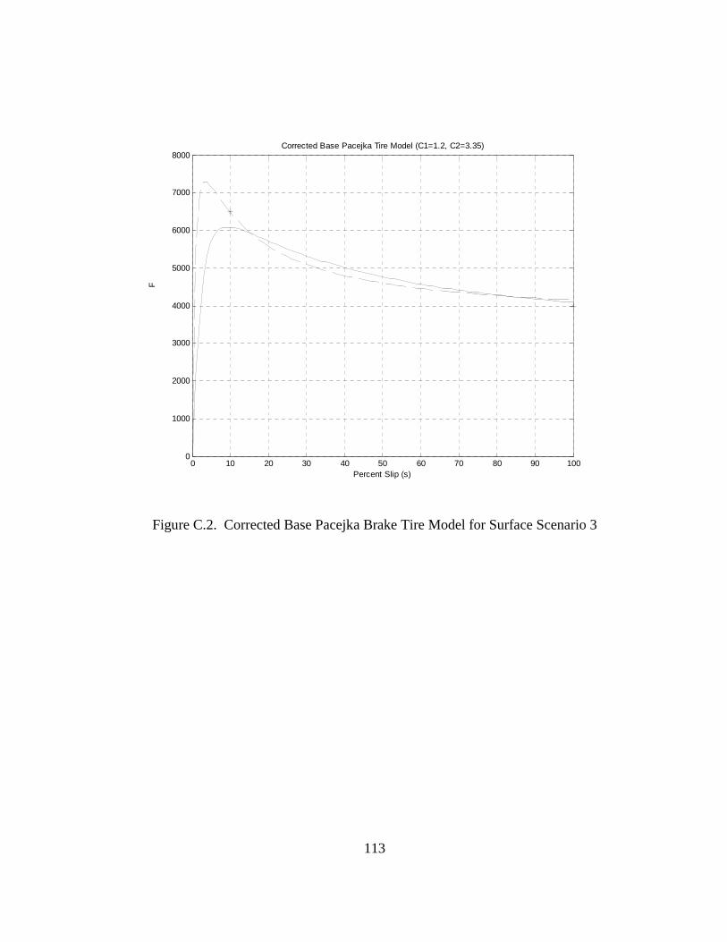
113

0 10 20 30 40 50 60 70 80 90 1000

1000

2000

3000

4000

5000

6000

7000

8000

Percent Slip (s)

FCorrected Base Pacejka Tire Model (C1=1.2, C2=3.35)

Figure C.2. Corrected Base Pacejka Brake Tire Model for Surface Scenario 3

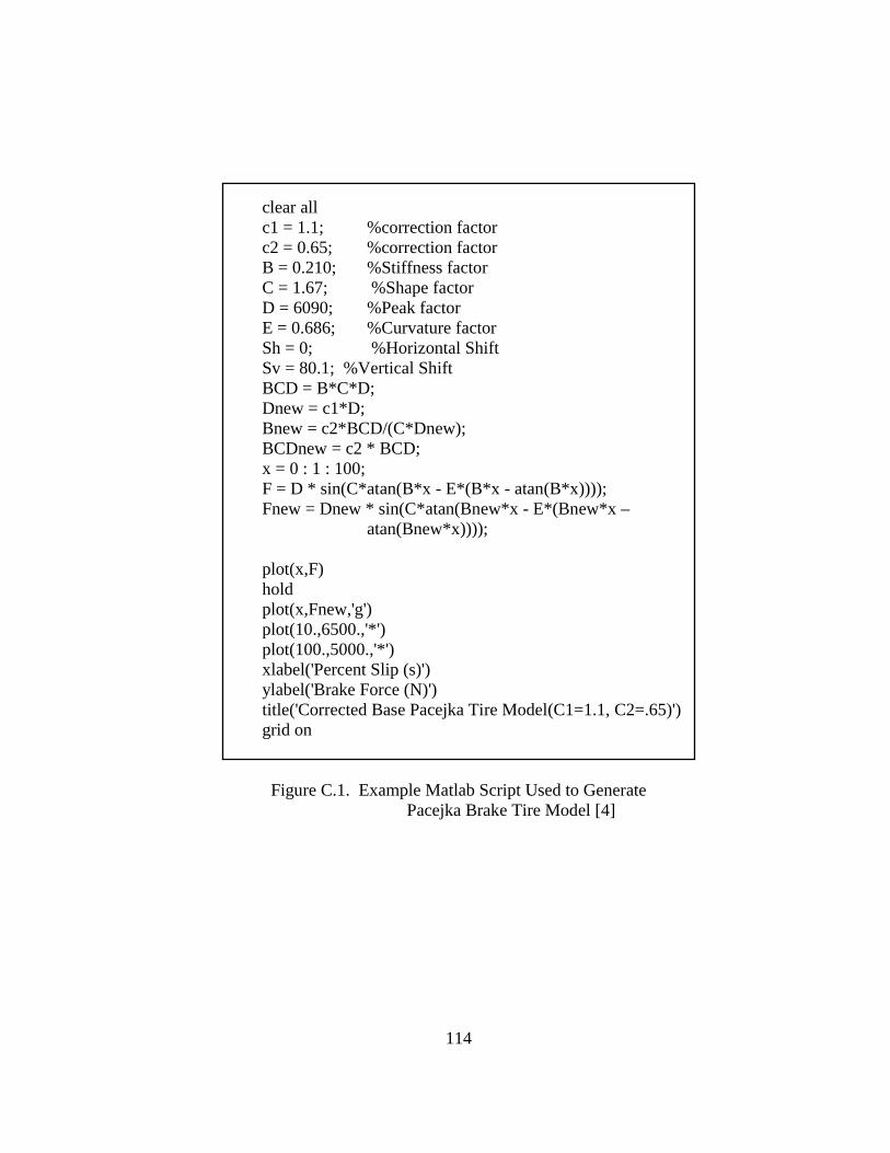
114

clear all c1 = 1.1; %correction factor c2 = 0.65; %correction factor B = 0.210; %Stiffness factor C = 1.67; %Shape factor D = 6090; %Peak factor E = 0.686; %Curvature factor Sh = 0; %Horizontal Shift Sv = 80.1; %Vertical Shift BCD = B*C*D; Dnew = c1*D; Bnew = c2*BCD/(C*Dnew); BCDnew = c2 * BCD; x = 0 : 1 : 100; F = D * sin(C*atan(B*x - E*(B*x - atan(B*x)))); Fnew = Dnew * sin(C*atan(Bnew*x - E*(Bnew*x –

atan(Bnew*x)))); plot(x,F) hold plot(x,Fnew,'g') plot(10.,6500.,'*') plot(100.,5000.,'*') xlabel('Percent Slip (s)') ylabel('Brake Force (N)') title('Corrected Base Pacejka Tire Model(C1=1.1, C2=.65)') grid on

Figure C.1. Example Matlab Script Used to Generate

Pacejka Brake Tire Model [4]

115

References

[1] R.S. Sharp, H.B. Pacejka, Shear Force Developmentby Pneumatic Tyres in Steady State Conditions: A Review of Modeling Aspects, Vehicle System Dynamics, 20, 1991, pp. 121-176.

[2] J.C. Dixon, Tyre, Suspension and Handling, Cambridge University Press,

Cambridge, 1991. [3] P. Van der Jagt, A.W. Parsons, Road Surface Correction of Tire Test Data,

Vehicle System Dynamics, 25, 1996, pp. 147-165. [4] H.B. Pacejka, E. Bakker, L. Nyborg, Tyre Modeling for Use in Vehicle

Dynamic Studies, Society of Automotive Engineers, 870421 & 890087, 1987. [5] B. Michalk, Texas Department of Transportation Construction and Pavement

Division, Personal Communication, 2002. [6] J.J. Henry, Tire Wet-Pavement Traction Measurement: A State-of-the-Art

Review, The Tire Pavement Interface, ASTM STP 929, 1986, pp. 3-25. [7] K.C. Ludema, Friction, Wear, Lubrication: A Textbook in Tribology, CRC

Press, New York, 1996. [8] D.F. Moore, The Friction of Pneumatic Tyres, Elsevier Scientific Publishing

Company, Amsterdam, 1975. [9] C.K. Kennedy, A.E. Young, I.C. Butler, Measurement of Skidding Resistance

and Surface Texture and the Use of results in the United Kingdom, Surface Characteristics of Roadways: International Research and Technologies, ASTM STP 1031, 1990, pp. 87-102.

[10] H. Takino, N. Isobe, H. Tobori, and S. Kohjiya, Effect of Cohesion Loss Factor

on Wet Skid Resistance of Tread Rubber, Tire Science and Technology, Vol. 26, No. 3, 1998, pp. 258-276.

[11] T. Gillespie, Fundamentals of Vehicle Dynamics, Society of Automotive

Engineers, 1992. [12] K. Yi, T. Jeoung, Road Friction Estimation Using Wheel Speed Sensors, 5th

World Congress on ITS, 1998.

116

[13] H.B. Pacejka, I.J.M. Besselink, Magic Formula Tyre Model with Transient Properties, Vehicle System Dynamics Supplement, 27, 1997, pp. 243-249.

[14] P. Bayle, J.F. Forissier, S. Lafon, A New Tyre Model for Vehicle Dynamics

Simulations, Automotive Technology International, 1993, pp. 193-198. [15] B. T. Kulakowski, M. Chi, C. Lin, Measurement and Modeling of Truck Tire

Traction Characteristics, Vehicle, Tire, Pavement Interface, ASTM STP 1164, 1992, pp. 112-124.

[16] R. R. Hegmon, Some Results from Ongoing Research on Road Roughness,

Vehicle, Tire, Pavement Interface, ASTM STP 1164, 1992, pp. 14-31. [17] K.C. Ludema, B.D. Gujrati, An Analysis of The Literature on Tire-Road Skid

Resistance, ASTM STP 541, 1973. [18] D.W. Harwood, B.T. Kulakowski, Effect of Water Film thickness on Tire

Pavement Friction, Surface Characteristics of Roadways: International Research and Technologies, ASTM STP 1031, 1990, pp. 50-60.

[19] L. Domenichini, F. La Torre, A. Scalamandre, Possible Applications of

Pacejka’s Model to Analysis of Vehicle Pavement Interaction in Conditions of Reduced Friction, World Road Association (PIARC), www.piarc.org/pub/0105.i/tri-it-e.htm, 2000.

[20] T. Bachmann, The Importance of the Integration of Road, Tyre, and Vehicle

Technologies, World Road Association (PIARC), www.piarc.lcpc.fr/pub/0105.i/tri-de-e.htm, 1995.

[21] U.S. Department of Transportation, Federal Highway Administration, Office of

Highway Policy Information, Highway Statistics 1999, www.fhwa.dot.gov/ohim/hs99/.

[22] K. Guo, J. Sui, The Effect of Longitudinal Force and Vertical Load Distribution

on Tire Slip Properties, 25th FISITA Congress, no. 945087, Beijing, China, 1994.

117

Vita

Gilberto Lopez was born in El Paso, Texas on December 8, 1977. He was

married to Christina Valadez June 2, 2002. He is the son of Gilberto I. Lopez, an

architect living in New York City, and Concepcion H. Flores, an accountant living in

San Antonio, Texas. Upon graduation from T. C. Clark High School, San Antonio,

Texas, he entered Texas A&M University in College Station, Texas. His sophomore

year he transferred to the University of Texas at Austin where he completed his

Bachelor of Science Degree in Mechanical Engineering in December of 2000.

During his undergraduate program of study he interned at Ford Motor Company and

was awarded a scholarship to continue his academic work for a period of one

semester in mechanical engineering at the Universidad Pontificia de Comillas in

Madrid, Spain. In the spring of 2001, he entered The Graduate School at the

University of Texas at Austin.

Permanent Address: 3416 Robinson # D Austin, Texas 78722 This thesis was typed by the author.