Copyright by Dong Eun Seo 2007

Copyright

by

Dong Eun Seo

2007

The Dissertation Committee for Dong Eun Seo

certifies that this is the approved version of the following dissertation:

Noncertainty Equivalent Nonlinear Adaptive Control

and its Applications to Mechanical and Aerospace

Systems

Committee:

Maruthi R. Akella, Supervisor

David G. Hull

Robert H. Bishop

Glenn Lightsey

S. Joe Qin



Systems

by

Dong Eun Seo, B.S.M.E., M.S.

Dissertation

Presented to the Faculty of the Graduate School of

The University of Texas at Austin

in Partial Fulfillment

of the Requirements

for the Degree of

Doctor of Philosophy


August 2007

To my wife and family

Acknowledgments

I would like to thank my advisor, Professor Maruthi R. Akella for his advices and

encouragements during the dissertation research. He is the person who not only led

me to the field of control theory but guided me while I lost in study. I am sure

that what he taught me of philosophical way of thinking with his comprehensive

knowledge will be in my mind for the rest of my life.

I also would like to thank all my committee members, Professor David G.

Hull, Professor Robert H. Bishop, Professor Glenn Lightsey, and Professor S. Joe

Qin. They provided the foundation of my knowledge and gave me inspiration of how

to approach problems from various perspectives by lectures, seminars and classes.

There are other people that I want to express my gratitude. My friends and staffs in

ASE/EM department who supported my academic life and encouraged me in doing

my best.

I am always thankful to Professor Sang-Yong Lee in Korea Advanced Insti-

tute of Science and Technology (KAIST) who was my mentor and gave me a chance

to study aborad.

Finally, I want to give my sincere appreciation to my wife, Dr. Jiwon Kim,

who became my soul mate always standing beside me, and my family who made all

that I have possible. I wish to thank my father, mother, and sister for their love and

support. I wish I can do the same things to my son, Ryan, who was born during

my wife’s dissertation.

v

The present work was partially supported by the National Science Foundation

and NASA Goddard Spaceflight Center.

Dong Eun Seo


August 2007

vi



Systems

Publication No.

Dong Eun Seo, Ph.D.

The University of Texas at Austin, 2007

Supervisor: Maruthi R. Akella

Adaptive control has long focused on establishing stable adaptive control methods

for various nonlinear systems. Existing methods are mostly based on the certainty

equivalence principle which states that the controller structure developed in the de-

terministic case (without uncertain system parameters) can be used for controlling

the uncertain system along by adopting a carefully determined parameter estima-

tor. Thus, the overall performance of the regulating/tracking control depends on

the performance of the parameter estimator, which often results in the poor closed-

loop performance compared with the deterministic control because the parameter

vii

estimate can exhibit wide variations compared to their true values in general. In

this dissertation, we introduce a new adaptive control method for nonlinear systems

where unknown parameters are estimated to within an attracting manifold and the

proposed control method always asymptotically recovers the closed-loop error dy-

namics of the deterministic case control system. Thus, the overall performance of

this new adaptive control method is comparable to that of the deterministic control

method, something that is usually impossible to obtain with the certainty equiv-

alent control method. We apply the noncertainty equivalent adaptive control to

study application arising in the n degree of freedom (DOF) robot control problem

and spacecraft attitude control. Especially, in the context of the spacecraft atti-

tude control problem, we developed a new attitude observer that also utilizes an

attracting manifold, while ensuring that the estimated attitude matrix confirms at

all instants to the special group of rotation matrices SO(3). As a result, we demon-

strate for the first time a separation property of the nonlinear attitude control

problem in terms of the observer/controller based closed-loop system. For both the

robotic and spacecraft attitude control problems, detailed derivations for the con-

troller design and accompanying stability proofs are shown. The attitude estimator

construction and its stability proof are presented separately. Numerical simulations

are extensively performed to highlight closed-loop performance improvement vis-

a-vis adaptive control designs obtained through the classical certainty equivalence

based approaches.

viii

Contents

Acknowledgments v

Abstract vii

List of Figures xii

Chapter 1 Introduction 1

1.1 Adaptive Control Principle . . . . . . . . . . . . . . . . . . . . . . . 1

1.1.1 Model Reference Adaptive Control . . . . . . . . . . . . . . . 2

1.1.2 Indirect Adaptive Control . . . . . . . . . . . . . . . . . . . . 6

1.1.3 Noncertainty Equivalence Adaptive Control . . . . . . . . . . 10

1.2 Research Motivation . . . . . . . . . . . . . . . . . . . . . . . . . . . 13

Chapter 2 A New Adaptive Control with High Performance 16

2.1 Problem Definition . . . . . . . . . . . . . . . . . . . . . . . . . . . . 16

2.2 Adaptive Control Utilizing Attracting Manifold . . . . . . . . . . . . 17

2.2.1 Motivating Problem . . . . . . . . . . . . . . . . . . . . . . . 18

2.2.2 Transforming Error System Using Filter States . . . . . . . . 19

2.2.3 New Adaptive Control Scheme and Stability Proof . . . . . . 21

2.2.4 Attracting Manifold in Adaptation . . . . . . . . . . . . . . . 26

2.3 Combination with Smooth Projection Technique . . . . . . . . . . . 28

ix

Chapter 3 Application to Robot Arm Control Problem 34

3.1 Introduction . . . . . . . . . . . . . . . . . . . . . . . . . . . . . . . . 34

3.2 Problem Formulation . . . . . . . . . . . . . . . . . . . . . . . . . . . 36

3.3 Adaptive Control for Robot Arm System . . . . . . . . . . . . . . . . 37

3.4 Adaptive Control with Parameter Projection . . . . . . . . . . . . . 42

3.5 Numerical Simulations . . . . . . . . . . . . . . . . . . . . . . . . . . 46

3.5.1 Proposed Adaptive Control . . . . . . . . . . . . . . . . . . . 47

3.5.2 Proposed Control with Projection Mechanism . . . . . . . . . 54

Chapter 4 Attitude Tracking Control Problem with Unknown Inertia

Parameters 58

4.1 Introduction . . . . . . . . . . . . . . . . . . . . . . . . . . . . . . . . 59


4.3 Adaptive Attitude Tracking Control . . . . . . . . . . . . . . . . . . 65

4.4 Adaptive Control with Parameter Projection . . . . . . . . . . . . . 73


4.5.1 Proposed Control without Projection Mechanism . . . . . . . 77

4.5.2 Proposed Control with Projection Mechanism . . . . . . . . . 90

Chapter 5 Attitude Estimator with Known Angular Velocity 94

5.1 Introduction . . . . . . . . . . . . . . . . . . . . . . . . . . . . . . . . 94


5.3 Adaptive Attitude Estimation with Attracting Manifold . . . . . . . 99

5.3.1 Main Result . . . . . . . . . . . . . . . . . . . . . . . . . . . . 99

5.3.2 Robustness Analysis . . . . . . . . . . . . . . . . . . . . . . . 101

5.3.3 Comparison with Certainty Equivalence Framework . . . . . 102

5.4 2-D Attitude Estimation . . . . . . . . . . . . . . . . . . . . . . . . . 104

5.5 3-D Attitude Estimation . . . . . . . . . . . . . . . . . . . . . . . . . 108

x


Chapter 6 Separation Property for the Rigid-Body Attitude Track-

ing Control Problem 122

6.1 Introduction . . . . . . . . . . . . . . . . . . . . . . . . . . . . . . . . 123

6.2 Full-state Feedback Control with True Attitude Values . . . . . . . . 125

6.3 Attitude Observer Design . . . . . . . . . . . . . . . . . . . . . . . . 132

6.4 Separation Property of Observer-based Attitude Control . . . . . . . 137


Chapter 7 Conclusions 148

7.1 Contributions . . . . . . . . . . . . . . . . . . . . . . . . . . . . . . . 148

7.2 Recommendations for Future Research . . . . . . . . . . . . . . . . . 150

Bibliography 152

Vita 160

xi

List of Figures

1.1 MRAC control scheme . . . . . . . . . . . . . . . . . . . . . . . . . . 3

1.2 Indirect adaptive control scheme . . . . . . . . . . . . . . . . . . . . 6

3.1 2-Link planar robot arm . . . . . . . . . . . . . . . . . . . . . . . . . 46

3.2 Tracking error norm trajectory along the time t . . . . . . . . . . . . 48

3.3 Parameter estimates trajectory of θ1(t) along the time t . . . . . . . 49



3.6 Control norm trajectory along the time t . . . . . . . . . . . . . . . . 53

3.7 Error norm trajectory comparison between the proposed method and

the proposed method with a projection . . . . . . . . . . . . . . . . 55

3.8 Parameter estimates trajectory comparison according to the existence

of a projection mechanism . . . . . . . . . . . . . . . . . . . . . . . . 56

3.9 Control trajectory comparison according to the existence of a projec-

tion mechanism . . . . . . . . . . . . . . . . . . . . . . . . . . . . . . 57

4.1 Reference signal property . . . . . . . . . . . . . . . . . . . . . . . . 78

4.2 Ideal case closed-loop performance obtained with the CE-based and

the proposed non-CE controller assuming the inertia matrix J to be

known . . . . . . . . . . . . . . . . . . . . . . . . . . . . . . . . . . . 80

xii

4.3 Adaptive attitude tracking closed-loop performance comparison be-

tween the classical CE-based controller and the proposed non-CE

controller for a non-PE reference trajectory . . . . . . . . . . . . . . 82

4.4 Performance study of the proposed non-CE adaptive attitude tracking

controller for two different different γ values . . . . . . . . . . . . . . 85

4.5 Ideal case closed-loop performance for the PE reference trajectory

obtained with the CE-based and the proposed non-CE controller as-

suming the inertia matrix J to be known . . . . . . . . . . . . . . . 87

4.6 Adaptive attitude tracking closed-loop performance comparison be-

tween the classical CE-based controller and the proposed non-CE

controller for a PE reference trajectory . . . . . . . . . . . . . . . . 89

4.7 Error norm trajectory comparison between the proposed method and

the proposed method with a projection . . . . . . . . . . . . . . . . 91

4.8 Parameter estimates trajectory comparison according to the existence

of a projection mechanism . . . . . . . . . . . . . . . . . . . . . . . . 93

5.1 Bounded Lyapunov candidate function for the attitude observer . . . 107

5.2 4-D hypersphere illustration for the attitude estimation error . . . . 113

5.3 The trajectory of the error quaternion z(t) with z(0) 6= 0 . . . . . . 119

5.4 The trajectory of the error quaternion z(t) with z(0) = 0 . . . . . . 120

5.5 The trajectory of the error quaternion z(t) with bounded measure-

ment noise . . . . . . . . . . . . . . . . . . . . . . . . . . . . . . . . . 121

6.1 Closed-loop simulation results comparing performance of the con-

troller from Eq. (6.41) (adopting the attitude estimator) with con-

troller from Eq. (6.12) that assumes direct availability of attitude

variables (no estimation required). . . . . . . . . . . . . . . . . . . . 144

xiii

6.2 Closed-loop simulation results comparing performance of the con-

troller from Eq. (6.41) (adopting the attitude estimator) with con-

troller from Eq. (6.12) that assumes direct availability of attitude

variables (no estimation required). The attitude estimator is initial-

ized in such a way that q(0) exactly satisfies condition q(0)Tq(0) = 0. 147

xiv

Chapter 1

Introduction

This chapter is devoted to basic concepts of adaptive control for further discussion

on the main results. At the beginning, two conventional adaptive control design

methods are explained, both of which are based on the certainty equivalence prin-

ciple. The following section discusses about noncertainty equivalence control based

on the analysis of differential topology. Motivation of the research is placed at the

end of this chapter.

1.1 Adaptive Control Principle

The control method that is able to adjust itself to unknown system parameters (cir-

cumstances) without sacrificing system stability is defined as the adaptive control.

Thus, adaptive control requires a systematic design tool for automatic adjustment of

itself in real time in order to achieve or maintain a desired control performance when

the system parameters are uncertain or varying in time. Because of the property

of the adaptive control, it has attracted increasing attention by both researchers

and practitioners. Since every system has unknown structure/parameters or dis-

turbances/defects in its dynamics virtually, verified and robust adaptive control

1

methods are always requested from diverse applications such as industrial robots,

aeromechanical systems, and underwater vehicles.

The definition (or concept) of adaptive control first appeared at 1950’s but

development of practical control methods (earlier conceptual design of model refer-

ence adaptive control) started in 1960’s[1], which is followed by an era of meaningful

theoretical progress in 1970’s and 1980’s (starting from Lyapunov theory and use of

Barbalat’s lemma). Nowadays, adaptive control is one of mature branch in control

theories and there exists a large amount of published literature on designing adaptive

controllers[2–4]. As a next phase of development, adaptive control confronts many

important challenges which include a faster response time for real-time applications,

a multi-agent cooperative control for flexible mission designs, a bio-mechanical con-

trol for continuously changing interaction with environments, etc. To cope with one

of those challenges, a high performance adaptive control is addressed throughout

this dissertation.

Based on the adaptation algorithm, conventional adaptive control methods

are broadly categorized into two groups: one is a direct adaptive control and the

other is an indirect adaptive control scheme. The term ‘direct’ and ‘indirect’ are

used to differentiate the relationship between the estimator for unknown system

parameters and the controller. In the following two sections, the detailed structure

of each control scheme is presented. In addition, a noncertainty equivalence adaptive

control is explained as a different approach to adaptation.

1.1.1 Model Reference Adaptive Control

Model reference adaptive control (also called a direct adaptive control) consists of

one unit which is used for control parameter adaptation and system control simul-

taneously. In Fig. 1.1, a schematic diagram of MRAC is shown.

A MRAC-type control law is designed as follows. First, the reference model

2

+

-

Adjustable ControllerPlant

Reference Model

u(t)=u(y(t),(e(t))) y(t)^

r(t)

y(t)=f(y(t),(t))

ym(t)

e(t)

Figure 1.1: MRAC control scheme

system should be identified wherein all the key performance requirements are con-

sidered and its feasibility on the actual system is guaranteed. Then, the control

structure is defined as if necessary control parameters are known. At this stage,

controller is parameterized by stabilizing control parameters φ∗ (usually a constant

or considered as a constant with slow-change assumption in time), not by unknown

system parameters θ∗. Finally, control parameter update law is designed and esti-

mates from control parameter estimator φ replace actual control parameters φ∗ in

the previously designed control law.

For example, consider the following first-order linear time-invariant plant

modified from [5]

y(t) = θ∗y(t) + bu(t), t > 0 (1.1)

where θ∗, b are unknown constant real system parameters, y(t) is a system output,

and u(t) is a control input. In addition, we assume b > 0 (in fact, this assumption on

b can be replaced with the relaxed assumption that the sign of b is known, but here

b > 0 for the simplicity). Then, the control objective is to design an adaptive control

input such that all closed-loop signals are bounded and y(t) tracks, asymptotically,

3

ym(t) given by

ym(t) = −amym(t) + r(t), t > 0 (1.2)

where am > 0. The stabilizing control law for the given system is expressed by

u(t) = −θ∗

by(t) +

1b

[−amy(t) + r(t)] , t > 0 (1.3)

Since both θ∗ and b are unknown, the structure of an adaptive controller is given by

ua(t) = φ1(t)y(t) + φ2(t) [−amy(t) + r(t)] (1.4)

which is designed with an assumption that stabilizing control parameter φ∗1 = − θ∗

b

and φ∗2 = 1b are known. Finding update laws for ˙

φ1(t) and ˙φ2(t)can be done in

various ways depending on design philosophies. However, for nonlinear systems (to

be handled in this dissertation), not much options are left and each design method

is sensitive to the system structure. Consider the following update laws for φ1(t)

and φ2(t):

˙φ1(t) =− γ1y(t)e(t) (1.5)

˙φ2(t) =− γ2 [−amy(t) + r(t)] e(t) (1.6)

where e(t) .= y(t) − ym(t) is a tracking error and γ1, γ2 > 0 are learning rates for

each update law. Then, we can show that e(t) → 0 as t → ∞ asymptotically by

analyzing the following Lyapunov candidate function

V =12e(t)2 +

b

2γ1φ1(t)

2+

b

2γ2φ2(t)

2(1.7)

where φ1(t).= φ1(t) −

(− θ∗

b

)and φ2(t)

.= φ2(t) − 1b are parameter estimation er-

rors. In the subsequent analysis, time argument ‘t’ is dropped off for the notational

4

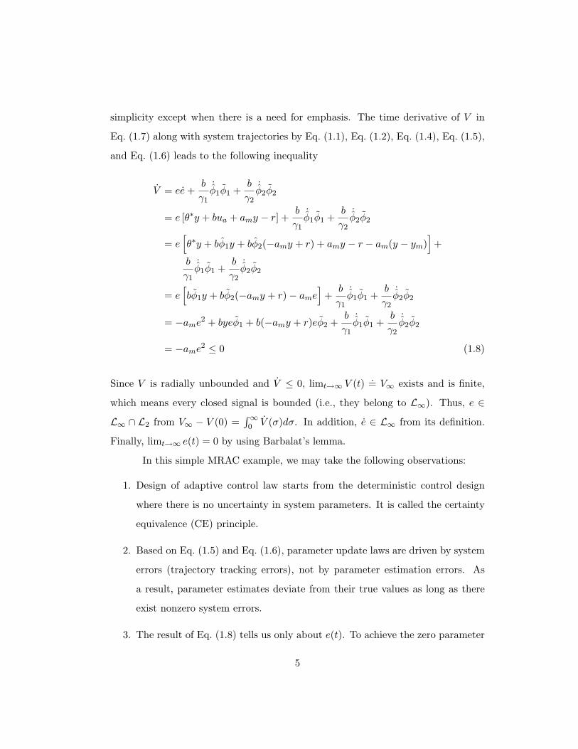
simplicity except when there is a need for emphasis. The time derivative of V in

Eq. (1.7) along with system trajectories by Eq. (1.1), Eq. (1.2), Eq. (1.4), Eq. (1.5),

and Eq. (1.6) leads to the following inequality

V = ee +b

γ1

˙φ1φ1 +

b

γ2

˙φ2φ2

= e [θ∗y + bua + amy − r] +b

γ1

˙φ1φ1 +

b

γ2

˙φ2φ2

= e[θ∗y + bφ1y + bφ2(−amy + r) + amy − r − am(y − ym)

]+

b

γ1

˙φ1φ1 +

b

γ2

˙φ2φ2

= e[bφ1y + bφ2(−amy + r)− ame

]+

b

γ1

˙φ1φ1 +

b

γ2

˙φ2φ2

= −ame2 + byeφ1 + b(−amy + r)eφ2 +b

γ1

˙φ1φ1 +

b

γ2

˙φ2φ2

= −ame2 ≤ 0 (1.8)

Since V is radially unbounded and V ≤ 0, limt→∞ V (t) .= V∞ exists and is finite,

which means every closed signal is bounded (i.e., they belong to L∞). Thus, e ∈

L∞ ∩ L2 from V∞ − V (0) =∫∞0 V (σ)dσ. In addition, e ∈ L∞ from its definition.

Finally, limt→∞ e(t) = 0 by using Barbalat’s lemma.

In this simple MRAC example, we may take the following observations:

1. Design of adaptive control law starts from the deterministic control design

where there is no uncertainty in system parameters. It is called the certainty

equivalence (CE) principle.

2. Based on Eq. (1.5) and Eq. (1.6), parameter update laws are driven by system

errors (trajectory tracking errors), not by parameter estimation errors. As

a result, parameter estimates deviate from their true values as long as there

exist nonzero system errors.

3. The result of Eq. (1.8) tells us only about e(t). To achieve the zero parameter

5

estimation error, reference trajectory ym(t) should satisfy certain condition

which is called the persistence excitation condition derived from Eq. (1.5) and

Eq. (1.6).

Listed characteristics are considered as common to CE-based control designs. In

the next section, we show the other adaptive control design philosophy based on the

certainty equivalence principle, that is expected to share the preceding properties of

CE-based control methods.

1.1.2 Indirect Adaptive Control

Different from MRAC (direct adaptive control), an indirect adaptive control scheme

consists of two parts: one is a system controller whose control parameters pretend

to be known (i.e., deterministic control design) and the other is a system parameter

estimator. Thus, in the indirect adaptive control method, system parameters are

estimated explicitly and then they are used to determine control parameters. In

Fig. 1.2, we can see an additional estimator between the system controller and the

plant in contrast with Fig. 1.1.

+

-

ControllerPlant

Reference Model

u(t)=u(e(t),((t))) y(t)

ym(t)

^ ^

r(t)

y(t)=f(y(t),(t))

^ ^

System Parameter Estimator

(t)=(e(t))e(t)

Figure 1.2: Indirect adaptive control scheme

6

Since this scheme is explicitly estimating the unknown system parameters,

we may have an extra information about the plant compared to the MRAC scheme.

To highlight the difference between the MRAC and the indirect adaptive control,

we use the same equation as Eq. (1.1), Eq. (1.2), and Eq. (1.3) as an example. Since

we have two unknown system parameters θ∗ and b, θ(t) and b are needed. The

corresponding adaptive controller is designed as follows

ua(t) =1

b(t)

[−θ(t)y(t)− amy(t) + r(t)

](1.9)

Therefore, in the indirect adaptive control scheme, adaptation is applied to a system

parameter and the task is to design both ˙θ(t) and ˙

b(t) which stabilize the overall

closed-loop system. Consider the following update laws:

˙θ(t) = γ1y(t)e(t) (1.10)

˙b(t) = γ2ua(t)e(t) (1.11)

where e(t) is the trajectory tracking error defined as before and γ1, γ2 > 0 are

learning rates for each update law (they play the same role as in MRAC). Next,

define the Lyapunov candidate function as follows

V =12e2 +

12γ1

θ +1

2γ2b (1.12)

where θ.= θ − θ∗ and b

.= b − b are parameter estimation errors. Then, taking

the time derivative of V in Eq. (1.12) along with Eq. (1.1), Eq. (1.2), Eq. (1.9),

7

Eq. (1.10), and Eq. (1.11) gives us

V = ee +1γ1

˙θθ +

1γ2

˙bb

= e [θ∗y + bua + amym − r] +1γ1

˙θθ +

1γ2

˙bb

= e[θ∗y − bua + bua + amy − r − ame

]+

1γ1

˙θθ +

1γ2

˙bb

= −ame2 − yeθ − uaeb +1γ1

˙θθ +

1γ2

˙bb

= −ame2 ≤ 0 (1.13)

If b 6= 0 for all t, then we may conclude that limt→∞ e(t) = 0 following the sim-

ilar arguments on closed-loop signal boundedness and Barbalat’s lemma as in the

previous MRAC section. Therefore, following observations are in order

1. As in the MRAC design, the control design is based on the deterministic

control case as in Eq. (1.3) for indirect adaptive control scheme. In other

words, the indirect adaptive controller also considers the estimated value as

the true system parameter. In other words, the indirect adaptive control

scheme is also developed based on the certainty equivalence principle.

2. Different from MRAC, each unknown system parameter is estimated explicitly.

Thus, the resultant structure of the indirect adaptive control law is identical

to the deterministic control law given in Eq. (1.3).

3. To implement Eq. (1.9), we need to guarantee b(t) 6= 0 for all t. This requires

the projection for b with an extra information of b (we already know b > 0).

8

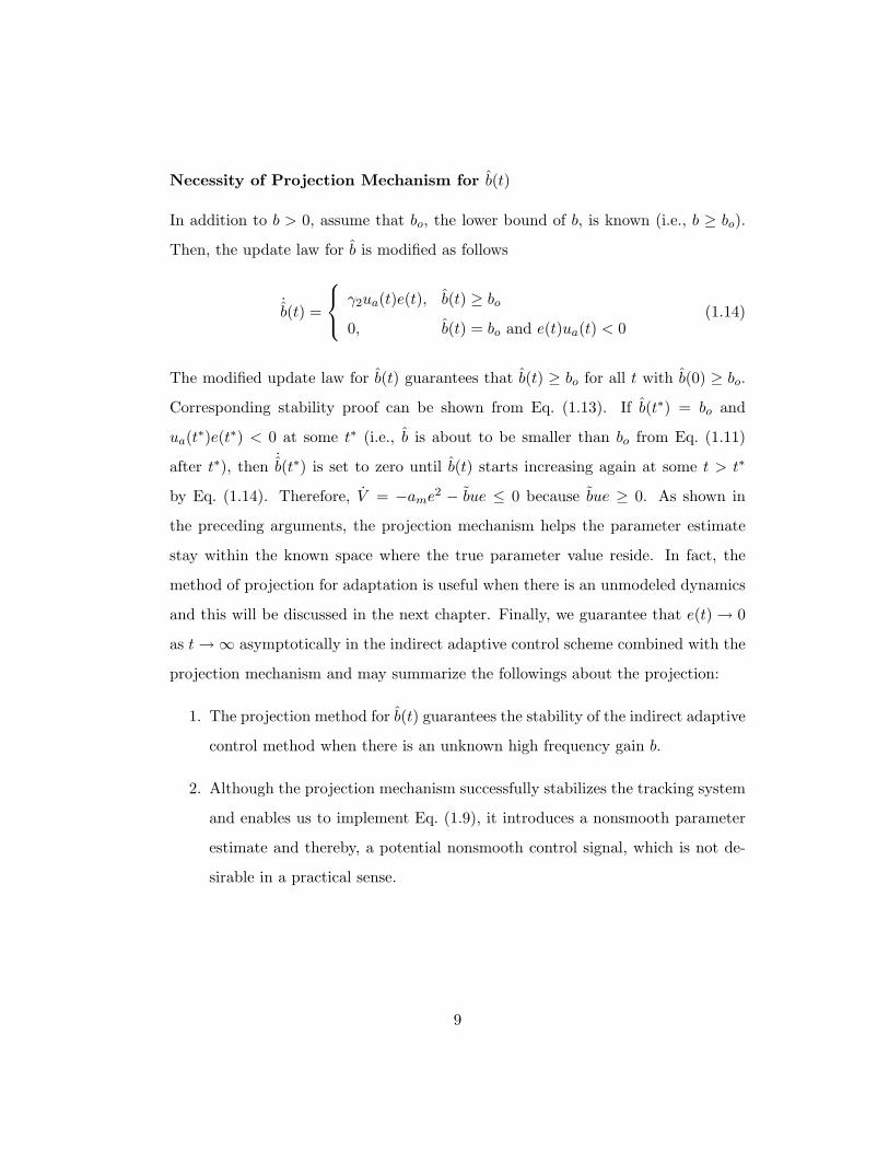
Necessity of Projection Mechanism for b(t)

In addition to b > 0, assume that bo, the lower bound of b, is known (i.e., b ≥ bo).

Then, the update law for b is modified as follows

˙b(t) =

γ2ua(t)e(t), b(t) ≥ bo

0, b(t) = bo and e(t)ua(t) < 0(1.14)

The modified update law for b(t) guarantees that b(t) ≥ bo for all t with b(0) ≥ bo.

Corresponding stability proof can be shown from Eq. (1.13). If b(t∗) = bo and

ua(t∗)e(t∗) < 0 at some t∗ (i.e., b is about to be smaller than bo from Eq. (1.11)

after t∗), then ˙b(t∗) is set to zero until b(t) starts increasing again at some t > t∗

by Eq. (1.14). Therefore, V = −ame2 − bue ≤ 0 because bue ≥ 0. As shown in

the preceding arguments, the projection mechanism helps the parameter estimate

stay within the known space where the true parameter value reside. In fact, the

method of projection for adaptation is useful when there is an unmodeled dynamics

and this will be discussed in the next chapter. Finally, we guarantee that e(t) → 0

as t →∞ asymptotically in the indirect adaptive control scheme combined with the

projection mechanism and may summarize the followings about the projection:

1. The projection method for b(t) guarantees the stability of the indirect adaptive

control method when there is an unknown high frequency gain b.

2. Although the projection mechanism successfully stabilizes the tracking system

and enables us to implement Eq. (1.9), it introduces a nonsmooth parameter

estimate and thereby, a potential nonsmooth control signal, which is not de-

sirable in a practical sense.

9

1.1.3 Noncertainty Equivalence Adaptive Control

Besides MRAC and indirect adaptive control schemes, a different approach to adap-

tive control problems is suggested[6] and its applications are presented[7–9], which is

called an immersion and invariance (I&I) control. Immersion is a mapping between

manifolds whose derivative is injective everywhere. In usual, immersion is defined

from the higher dimensional manifolds to the lower dimensional manifold for the

mapping to be injective (i.e., nonsingular map). In the context of the adaptive

control design, immersion is used to transform the given nonlinear system involving

parameter estimate into the reduced order dynamics (target dynamics) in terms of

system states which is locally/globally stable with respect to the equilibrium points.

In spite of benefits from immersion such as smooth control trajectory, there is a

major restriction for it to be applied to general nonlinear systems. The nonlinearity

of closed-loop dynamics should also have an attractive implicit manifold as well as a

proper immersion[6] where the implicit manifold represents the unknown parameter

adaptation . By the following example, each concepts in I&I control method are

demonstrated. Consider the following nonlinear trajectory tracking control system

y(t) = y2(t)︸︷︷︸f(y(t))

θ∗ + u(t), t > 0 (1.15)

where θ∗ is an unknown system parameter and f(y) is a regressor for the system

parameter θ∗. We denote the reference trajectory as ym(t) as before. Since θ∗ is

unknown, entire error system including adaptation is represented as follows

Σ :

e(t) = f(y(t))θ∗ + u(t)− ym(t)˙θ(t) = β2(t)

(1.16)

10

where e(t) .= y(t)− ym(t) and β2(t) will be determined. An I&I controller proposed

by [6] is given as

u(t) = −e(t)− f(y(t))[θ(t) + β1(y(t))

]+ ym(t) (1.17)

If we can find β1(y) satisfying the following

∂β1(y)∂y

f(y) +[∂β1(y)

∂yf(y)

]T

> 0 (1.18)

then, β2(t) is determined and the closed-loop system is asymptotically stable. Con-

sider the following Lyapunov candidate function

V =12e2 +

12γ

z2 (1.19)

where z.= θ + β1 − θ∗ and γ > 0. Then, by taking the time derivative of V in

Eq. (1.19) along with Eq. (1.16) and Eq. (1.17), we have

V = e(−e− y2z) +1γ

z

[˙θ +

∂β1

∂y(−e− y2z + ym)

]= e(−e− y2z) +

1γ

z

[β2(t) +

∂β1

∂y(−e− y2z + ym)

](1.20)

Now, choose β1(y) as

β1(y) =γ

3y3 (1.21)

which satisfies Eq. (1.18) obviously. Subsequently, β2(t) is determined as

β2(t) = γy2(y − ym − ym) (1.22)

11

Substituting Eq. (1.21) and Eq. (1.22) into Eq. (1.20) leads to the following inequal-

ity

V = −e2 − ey2z − y4z2

= −12e2 − 1

2y4z2 − 1

2(e + y2z)2

≤ −12e2 − 1

2y4z2 (1.23)

Since V is radially unbounded and V ≤ 0, limt→∞ V (t) .= V∞ exists and is finite.

Thus, e, z ∈ L∞. From∫∞0 V (σ)dσ = V∞−V (0), e, y2z ∈ L ∈ L2∩L∞. In addition,

e, ddt(y

2z) ∈ L∞. Therefore, by Barbalat’s lemma, limt→∞[e, y2z] = 0. For the given

nonlinear system Eq. (1.16), the immersion π is defined as

π : [e] →

e

θ∗ − β2(e)

(1.24)

where β2(e) is just coordinate transformation of β2(t). The corresponding implicit

manifold is z = 0 and its manifold attractivity is given by

z = −γy4z (1.25)

Target dynamics for Eq. (1.16) are e = −e which can always be achieved since the

disturbance term y2z of the closed-loop dynamics (e = −e− y2z) goes to zero.

In fact, solving Eq. (1.18) requires fT (y) be integrable. Because f(y) is

scalar, it is always possible to find such β1(y) that Eq. (1.18) is satisfied. However,

Eq. (1.18) is not solvable for general multidimensional nonlinear f(y). For linear

systems, these requirements are easily bypassed by adopting state filters[9].

12

1.2 Research Motivation

Based on the previous research survey, the existing adaptive control methods using

a certainty equivalence principle suffer from performance degradation due to the

following aspects:

1. As shown in preceding examples for MRAC and indirect adaptive control

schemes, both system error dynamics share the following structure

e = −ame︸︷︷︸target dynamics

+disturbance (1.26)

wherein ‘disturbance’ term converges to zero only when parameter estimates

coincide with their true values if e 6= 0. Therefore, the overall closed-loop sys-

tem performance is ultimately determined by the performance of the parame-

ter estimator, which is poor without a persistently exciting reference trajectory

(the PE reference trajectory is defined as a signal that can derive parameter

estimates to true parameter values in section 1.1.1).

2. The parameter update law involves no estimation error term and is driven by

the regulation/tracking error of the system. This leads to the fact that the es-

timator keeps generating update signals even when estimates are equal to true

parameters as long as the regulation/tracking error has nonzero values. In the

same context, the parameter update stops whenever the regulation/tracking

error becomes zero although parameter estimates are away from true param-

eters. Consequently, the structure of the adaptation algorithm also degrades

the overall closed-loop system performance.

3. The closed-loop dynamics controlled by the certainty equivalence principle are

unable to recover the deterministic control system dynamics although the reg-

ulation/tracking error converges to zero asymptotically. This recovery of the

13

error dynamics happens only when estimates are exactly equal to true pa-

rameters since the certainty equivalence principle is based on the cancelation

of uncertain parameter effects. The exact cancelation of uncertain parameter

effects never happens in actual applications. Therefore, the certainty equiva-

lence control never achieves its theoretical best performance in the long run.

4. An attempt to improve the performance of certainty equivalence based control

methods by increasing the learning rate results in the large amount of control

efforts. Thus, increasing the learning rate is limited by the practical issue on

implementation.

5. The I&I control method shows a potential to improve aforementioned prob-

lems of the certainty equivalence principle, but it is not applicable to general

nonlinear systems because of a strong restriction due to the integrability con-

dition.

Motivated by those observations, we address the high performance adaptive

control method by introducing an attracting manifold into adaptation while main-

taining global asymptotic stability. The key issue is how to eliminate the integra-

bility restriction and thereby improve the overall system performance with general

nonlinearities. To resolve the integrability issue, we introduce a regressor filter. The

regressor filter enables us to transform the closed-loop dynamics into the filtered

system dynamics wherein states are given by filtering states of the original closed-

loop dynamics. Further, the filtered error dynamics make it possible to construct a

strict Lyapunov function, which, in turn, helps to provide a separation property for

certain classes of nonlinear observer-based adaptive control systems.

The rest of the dissertation is organized as follows. In Chap. 2, the main

results and analysis are presented. Then, as an application of the proposed control

method, a robot arm trajectory control problem and an attitude tracking control

14

problem are solved in Chap. 3 and Chap. 4, respectively. Through Chap. 5 and

Chap. 6, the attitude tracking problem is addressed more specifically involving a

new attitude observer and a separation property for the proposed attitude observer

and the controller. Finally, summary and contributions of the present work are

presented in Chap. 7.

15

Chapter 2

A New Adaptive Control with

High Performance

In this chapter, we introduce a new control method which is not using the certainty

equivalence principle. As mentioned in the previous chapter, certainty equivalence

control depends on the cancelation of uncertain parameter effects. Thus, it has

limited transient performance because cancelation is not always exact. The pro-

posed control method overcomes this transient performance limitation by adopting

an attracting manifold and enables the controlled system to recover the transient

performance of deterministic control regardless of unknown parameter effects. This

chapter contains the derivation of main theoretical results, stability proof, and dis-

cussions about its properties.

2.1 Problem Definition

The generalized system representation in the state space form is given by

x(t) = F (x(t),θ∗,u(t)) (2.1)

16

where F describes the vector field, x(t) ∈ Rn is a state vector, θ∗ ∈ Rm is an

m-dimensional constant unknown system parameter vector, and u(t) ∈ Rp is a p-

dimensional control input. For the simplicity of notation, the time argument t is

omitted except when we need to emphasize it in the context. To reduce this general

system in Eq. (2.1) into the manageable form, we need the following assumption.

Assumption 1. System equation given in Eq. (2.1) has the parameter affine rep-

resentation in general sense.

In Assumption 1, “general sense” means that the original system of Eq. (2.1)

can have the nonlinearly parameterized representation as long as it can be linearly

parameterized using overparametrization. Under Assumption 1, we consider the

systems which have the following parameter affine representation throughout this

dissertation.

x = f(x)θ∗ + Φ∗g(x)u (2.2)

where f(x) ∈ Rn×m is a regressor matrix and g(x) ∈ Rn×p is a control mapping

matrix. In addition to the parameter affine system assumption, we are also in need

of the controllability assumption stated as follows:

Assumption 2. Φ∗ > 0 and g(x) in Eq. (2.2) have a full rank with respect to the

control input u

In other words, we disregard the uncontrollable system. One more thing need

to be mentioned is that linear systems always can be expressed as in Eq. (2.2), we

focus only on nonlinear systems hereafter.

2.2 Adaptive Control Utilizing Attracting Manifold

This section contains the new control method and its stability proof for the sim-

plified system with the analysis of the attracting manifold used in the parameter

adaptation.

17

2.2.1 Motivating Problem

To highlight the effect of attracting manifold in adaptation, the controllability con-

dition of Eq. (2.2) for g(x) is simplified by replacing g(x) with an identity matrix.

However, this simplification will not hurt our result because we already assumed

that g(x) has a full rank with respect to the control input u. Thus, the following

system equation is considered.

x = f(x)θ∗ + Φ∗u (2.3)

Our control objective is to make the system of Eq. (2.3) follow the reference trajec-

tory xm. Thus, to quantify the error between the system state x and the reference

state xm, we define the following error vector e as

e = x− xm (2.4)

Then, the control objective rendered in error vector space can be restated as follows:

Tracking control objective is to make e go to zero as time passes, where e has the

following dynamics.

e = f(x)θ∗ + Φ∗u− xm (2.5)

In followings, we develop a nonlinear controller that ensures the satisfaction of the

tracking control objective for e whose dynamics is given by Eq. (2.5).

18

2.2.2 Transforming Error System Using Filter States

Before we proceed to the synthesis of the proposed controller, following filter states

need to be defined.

ef = −αef + e (2.6)

Wf (t) = −αWf (t) + W (x, xm) (2.7)

uf = −αuf + u (2.8)

where α > 0 and W (x, xm) is defined from the following relationship.

W (x, xm)ψ∗ = Φ∗−1f(x)θ∗ − Φ∗−1xm + kΦ∗−1e (2.9)

with k > 0 and a new unknown constant vector ψ∗ ∈ Rn(n−1)(m+1)/2 having mixed

parameters from both θ∗ and Φ∗−1. Since xm is assumed to be known reference

information, we denote W (x, xm) as W (x) for the notational simplicity. From the

definition of filter states, the following observations are in order.

1. Although Φ∗ is a constant unknown matrix, we already assumed that it is a

positive definite matrix in Eq. (2.1). Thus, the existence of Φ∗−1 is always

guaranteed.

2. In addition to the error filter ef of Eq. (2.6), a regressor filter Wf of Eq. (2.7)

is newly introduced because of the integrability issue mentioned in the pre-

vious chapter. This regressor filter enables us to eliminate the integrability

conditions posed by [6, 9], which will be explained in the following section.

3. Introduced control filter uf of Eq. (2.8) does not have to be included for actual

implementation for u. After uf is defined in terms of either original states

in Eq. (2.5) or filter states, u can be easily recovered using the filter state

definition. Thus, the control filter of Eq. (2.8) is used only for the analysis.

19

4. The dimension of ψ∗ in Eq. (2.9) is maximal in a sense that it is derived based

on overparametrization. It can be smaller than expected depending on the

actual application as presented in the later chapter.

5. α is a filter gain which regulate filter response to system states. By increasing

α, we can make filter states converge to the system states more rapidly.

6. k is a proportional gain of the proposed controller described in the next section.

Based on these filter definitions, Eq. (2.6), Eq. (2.7) and Eq. (2.8), we derive the

following lemma to synthesize the new control scheme.

Lemma 1 (Dynamics of Filter States). The following filtered system dynamics are

equivalent to the error dynamics of Eq. (2.5) in a sense that if ef (t) → 0 as t → 0,

then limt→∞ ef = 0 ⇔ limt→∞ e = 0.

ef = −kef + Φ∗ [Wf (t)ψ∗ + uf ] (2.10)

Proof. Filter states defined from Eq. (2.6) to Eq. (2.8) are used to transform the

error dynamics of Eq. (2.5) into the filtered error dynamics of Eq. (2.10). First, we

have to rearrange the error dynamics in Eq.(2.5) to get a regressor matrix defined

in Eq.(2.9). The error system dynamics of Eq.(2.5) is rewritten as follows:

e = −ke+ Φ∗[Φ∗−1f(x)θ∗ − Φ∗−1xm + kΦ∗−1e+ u

]= −ke+ Φ∗ [W (x)ψ∗ + u] (2.11)

By substituting each filter definition into Eq. (2.11) and rearranging terms properly,

we get the following differential equation.

d

dt[ef + kef − Φ∗ (Wf (t)ψ∗ + uf )] = −α [ef + kef − Φ∗ (Wf (t)ψ∗ + uf )] (2.12)

20

which is the simple first order differential equation. Since the solution for Eq. (2.12)

exponentially converges to zero, the term inside the square bracket can be expressed

as follows:

ef = −kef + Φ∗ [Wf (t)ψ∗ + uf ] + ε(t) (2.13)

where ε(t) .= ε(0)e−αt represents the exponentially decaying term given by

ε(t) = −αε(t); ε(0) = [ef + kef − Φ∗ (Wf (t)ψ∗ + uf )]t=0 (2.14)

Thus, Eq. (2.10) is derived by setting ε(0) = 0 because the initial value of each filter

state can be chosen arbitrarily. Finally, proof of the stability equivalence between

ef and e is done simply by noticing that both sides of Eq. (2.6) should go to zero

as t goes to infinity.

It is clear from the above result that the control input u should be synthesized

to ensure the convergence of both ef and ef to zero. In other words, uf need

to be designed to make both ef and ef go to zero as t goes to infinity. Ignoring

exponentially decaying additive terms during stability analysis is somewhat standard

practice among the adaptive control research community[10, 11] as in Eq. (2.10).

However, the previous lemma should be applied carefully in the general case of

cascaded systems involving exponentially decaying terms[12].

2.2.3 New Adaptive Control Scheme and Stability Proof

We propose a new adaptive control scheme in this section. The proposed control

method performs adaptation on the attracting manifold. As a result, deterministic

control system dynamics are recovered by the attracting manifold, not by the cance-

lation of unknown parameter effects which is the principle of the certainty equivalent

control scheme. After we show the structure of the controller, the stability proof is

presented.

21

Theorem 1 (Adaptive Full-state Feedback Control). Consider the tracking control

problem whose error dynamics can be represented by Eq. (2.5). Then, the control

input u computed by the following update law with filters defined by Eq. (2.6) and

Eq. (2.7) guarantees the global stability and the satisfaction of the control objective

described by the asymptotic tracking error convergence, limt→∞ e(t) = 0, for any

initial condition.

u = −W (x)(θ + β)− γWf (t)W Tf (t) [(k − α)ef + e] (2.15)

where γ > 0 is an adaptive gain, k and W (x) are from Eq. (2.9), and α is the same

α as in the filter definition. Each θ and β is generated by the following relationships:

˙θ(t) = γ(k + α)W T

f (t)ef − γW T (x)ef (2.16)

β = γW Tf (t)ef (2.17)

The estimates of unknown parameters are given by θ + β.

Proof. This stability proof consists of three steps. First, the original tracking error

system is transformed into the filtered error system. Second, the proposed con-

trol input uf is synthesized based on the filtered error system. Finally, the global

asymptotic stability for the filtered error system is proved using Lyapunov candidate

function and the actual control input u is recovered from uf .

Using filter states in Eq. (2.6) and Eq. (2.7), we get the filtered error system

Eq. (2.10) in Lemma 1 from Eq. (2.5) along with the regressor W (x) in Eq. (2.9).

To make sure that ε(t) = 0 for all t > 0, we set the filter initial value as ef (0) =

e(0)/(α − k) and Wf (0) = 0. Since α − k is the denominator of ef (0), α and k

should be chosen properly. By transforming the error system of Eq. (2.5) into the

filtered error system of Eq. (2.10), we can always construct β function instead of

finding one which is satisfying the condition in Eq. (1.18) because, as mentioned

22

earlier, a solution to Eq. (1.18) for most of nonlinear regressor matrix W (x) is not

available in general. Next, control input uf is designed as follows

uf = −Wf (t)(θ + β) (2.18)

where θ and β are from Eq. (2.16) and Eq. (2.17). By substituting Eq. (2.18) into

the filtered error system Eq. (2.10), we obtain the following simplified dynamics for

ef .

ef = −kef − Φ∗Wf (x)z (2.19)

where z represents the error vector between the estimates and the true parameters

defined by

z = θ + β −ψ∗ (2.20)

If we can show that both ef (t) and ef (t) go to zero as t goes to infinity, then we

prove limt→∞ e(t) = 0 by Lemma 1. As the final step of our proof, consider the

following Lyapunov candidate function.

V =12eT

f ef +ζ

2λminzTz (2.21)

where ζ is any positive number that satisfies ζ > 12kγ and λmin is the smallest eigen-

value of 12(Φ∗−T + Φ∗−1). The time derivative of V evaluated along the trajectory

generated from Eq. (2.19) can be simplified together with Eq. (2.16) and Eq. (2.17)

23

as follows:

V = eTf (−kef − Φ∗Wfz) +

ζ

λminzT( ˙θ + β

)= −keT

f ef − eTf Φ∗Wfz +

ζ

λminzT[ ˙θ + γW T

f ef + γW Tf ef

]6 −k‖ef‖2 + ‖ef‖‖Φ∗Wfz‖ − ζγ‖Φ∗Wfz‖2

6 −k

2‖ef‖2 −

ζγ

2‖Φ∗Wfz‖2 −

k

2

[‖ef‖2 −

2k‖ef‖‖Φ∗Wfz‖+

2ζγ

k‖Φ∗Wfz‖2

]︸︷︷︸

>0 from ζ definition

6 −k

2‖ef‖2 −

ζγ

2‖Φ∗Wf (t)z‖2 (2.22)

which means that V (t) is negative semi-definite. Thus, V (t) ∈ L∞, which imply

all signals (ef , z, and Wf ) are bounded. Based on the structure of each filter, the

boundedness of all filtered signals is equivalent to the boundedness of all closed loop

signals in Eq.(2.5) since xm might be assumed as a bounded reference signal without

loss of generality. In addition to the boundedness of V (t) for all t ≥ 0, there exists

V∞ such that limt→∞ V (t) = V∞ < ∞. Since V∞ − V (0) = limt→∞∫ t0 V (σ)dσ,

ef ∈ L2. Therefore, ef ∈ L2∩L∞. Furthermore, we see that ef ∈ L∞ and ef ∈ L∞

from Eq. (2.6) and Eq. (2.19), which implies limt→∞[ef (t), ef (t)] = 0 by applying

Barbalat’s lemma recursively. This proves the global asymptotic stability of the

proposed control scheme with the help of Lemma 1. The actual control input u is

recovered from Eq. (2.8) as follows:

u = uf + αuf

= −Wf

[θ + β

]−Wf

[ ˙θ + β

]− αWf

[θ + β

]= −W (x)

[θ + β

]−Wf

[ ˙θ + β

](2.23)

which is identical to Eq.(2.15) when Eq.(2.6), Eq.(2.7), Eq.(2.16) and Eq.(2.17) are

24

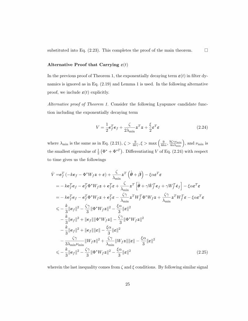
substituted into Eq. (2.23). This completes the proof of the main theorem.

Alternative Proof that Carrying ε(t)

In the previous proof of Theorem 1, the exponentially decaying term ε(t) in filter dy-

namics is ignored as in Eq. (2.19) and Lemma 1 is used. In the following alternative

proof, we include ε(t) explicitly.

Alternative proof of Theorem 1. Consider the following Lyapunov candidate func-

tion including the exponentially decaying term

V =12eT

f ef +ζ

2λminzTz +

ξ

2εTε (2.24)

where λmin is the same as in Eq. (2.21), ζ > 94kγ , ξ > max

(9

4kα , 9ζγνmin4αλmin

), and νmin is

the smallest eigenvalue of 12

(Φ∗ + Φ∗T

). Differentiating V of Eq. (2.24) with respect

to time gives us the followings

V =eTf (−kef − Φ∗Wfz + ε) +

ζ

λminzT( ˙θ + β

)− ξαεTε

=− keTf ef − eT

f Φ∗Wfz + eTf ε+

ζ

λminzT[ ˙θ + γW T

f ef + γW Tf ef

]− ξαεTε

=− keTf ef − eT

f Φ∗Wfz + eTf ε−

ζγ

λminzT W T

f Φ∗Wfz +ζγ

λminzT W T

f ε− ξαεTε

6− k

3‖ef‖2 −

ζγ

3‖Φ∗Wfz‖2 −

ξα

3‖ε‖2

− k

3‖ef‖2 + ‖ef‖‖Φ∗Wfz‖ −

ζγ

3‖Φ∗Wfz‖2

− k

3‖ef‖2 + ‖ef‖‖ε‖ −

ξα

3‖ε‖2

− ζγ

3λminνmin‖Wfz‖2 +

ζγ

λmin‖Wfz‖‖ε‖ −

ξα

3‖ε‖2

6− k

3‖ef‖2 −

ζγ

3‖Φ∗Wfz‖2 −

ξα

3‖ε‖2 (2.25)

wherein the last inequality comes from ζ and ξ conditions. By following similar signal

25

chasing procedure described in the previous proof of Theorem 1 and using Barbalat’s

lemma, we guarantee that limt→∞[ef (t),Wf (t)z(t), ε(t)] = 0. In addition, by ef =

−kef − Φ∗Wfz + ε, we have limt→∞ ef (t) = 0. Finally, we obtain limt→∞ e(t) = 0

from Eq. (2.6) as expected.

In this section, we discussed about the global asymptotic stability of the

proposed controller and stability proof was given in two ways. Either of them

(with/without ε(t) in filter dynamics) works fine. However, an attracting manifold

used in adaptation is not clearly defined and the role of the attracting manifold is

not shown either. In the following section, we clarify the attracting manifold in the

adaptive control method presented in Theorem 1 and investigate its properties in

the perspective of adaptation.

2.2.4 Attracting Manifold in Adaptation

An attracting manifold for adaptation is defined by the following lemma.

Lemma 2 (Attracting Manifold). For the given adaptive control system in Eq. (2.10)

with the control input uf of Eq. (2.18) along with Theorem 1, the adaptation error

z of Eq. (2.20) has an attracting manifold S such that

S = z | Wfz = 0 (2.26)

Proof. Consider the following Lyapunov candidate function from Eq. (2.21).

Vz =ζ

2λminzTz (2.27)

where ζ and λmin are the same as in Eq. (2.21). Taking the time derivative of

26

Eq. (2.27) lead us to the following inequality.

Vz =ζ

λminzT( ˙θ + β

)=

ζ

λminzT( ˙θ + W T

f ef + W Tf ef

)6 −ζγ‖Φ∗Wfz‖2 (2.28)

Last inequality is obtained by substituting Eq. (2.7), Eq. (2.16), and Eq. (2.19) into

Eq. (2.28). In a similar way of proving Theorem 1, we see that Vz ∈ L∞ as well as the

existence of Vz∞ such that limt→∞ Vz(t) = Vz∞ because Vz > 0 and Vz 6 0. Thus,

z ∈ L∞. In fact, all closed loop signals are already shown to be bounded by the

proof of Theorem 1. From Vz∞−Vz(0) = limt→∞∫ t0 Vz(σ)dσ, Wfz ∈ L2. Therefore,

Wfz ∈ L2 ∩ L∞. In addition, Wf , z ∈ L∞ from the boundedness of closed loop

signals. Using Barbalat’s lemma for Wfz ∈ L2 ∩ L∞ and ddt (Wfz) ∈ L∞, we may

conclude that Wfz → 0 as t →∞. This proves the attractiveness of S.

Remark 1. Using the attractiveness of S, we may prove the global stability in The-

orem 1. First, we prove that ef → 0 as t → ∞. Then, we may show that ef → 0

as t →∞ from Eq. (2.19) using Lemma 2. Finally, we claim e→ 0 as t →∞ from

Eq. (2.6).

Remark 2. Lemma 2 tells us that ef dynamics of Eq. (2.19) recovers ef = −kef all

the time, which results in the improvement of transient responses in e. On the other

hand, to achieve the control objective, the certainty equivalent controller relies upon

the cancelation of unknown parameter effects which is not exact.

Remark 3. z ∈ S does not mean z = 0 because Wf is not a full rank square matrix.

Thus, z on S may have a nonzero vector.

Remark 4. Although the convergence of z to zero is not guaranteed, z stays at zero

after the moment when θ + β hit the true parameter vector ψ∗. This may be clear

27

from the z dynamics

z = −γW Tf Φ∗Wfz (2.29)

which is different from the certainty equivalent control method where parameter esti-

mates always deviate from true values at the beginning of adaptation. This also helps

enhancing the performance of the proposed controller compared with the certainty

equivalent scheme because the new control method stops updating parameter esti-

mates after hitting true values while the conventional certainty equivalent method

keeps searching true values asymptotically. We must be careful about Eq. (2.29).

Eq. (2.29) is obtained only when ε(t) = 0 for all t ≥ 0. Otherwise, there exists an

extra term γW Tf ε in R.H.S. of Eq. (2.29) and we loose the nice feature (parameter

estimate stays locked at the true value after hitting it as long as ε(t) 6= 0). However,

it is always possible to choose the initial filter states such that ε(t) = 0 for all t ≥ 0

by setting ε(0) = 0 based on Eq. (2.14) using ef (0) = e(0)k−α and Wf (0) = 0.

2.3 Combination with Smooth Projection Technique

In the foregoing analysis, we do not investigate the robustness property of the pro-

posed control method when there exist unknown exogenous disturbances. It is well

known that even small bounded disturbances in the adaptively controlled system

may lead to the closed-loop system instability or deteriorate the closed-loop perfor-

mance significantly[13] because of the parameter drift (i.e., unbounded growth of

parameter estimates due to the disturbance). To resolve this problem, robustness

modification is applied to the system. Conventional robustness modification for the

systems with unknown external disturbances include adding a leakage term ( e.g.,

σ-modification and ε-modification)[14] or using projection for estimates to be con-

fined inside a bounded convex set where true parameters reside[13–16]. Since we

already present the projection technique in the indirect adaptive control example,

28

only σ-modification is demonstrated here. Suppose we have the following system

equation for regulation (i.e., we want that y(t) → 0 as t →∞)

y(t) = θ∗y(t) + u(t) + d(t) (2.30)

where d(t) is either unmodeled or external disturbance and θ∗ is unknown. By

following the conventional parameter update law and CE-based control design, we

have

u(t) =− y(t)− θ(t)y(t) (2.31)

˙θ(t) =γy2(t) (2.32)

Consider the following Lyapunov candidate function

V =12y2 +

12γ

θ2 (2.33)

where θ(t) .= θ(t) − θ∗ is a parameter estimation error and γ > 0. The time

derivative of V in Eq. (2.33) along with Eq. (2.31) and Eq. (2.32) leads to the

following inequality

V =y(−y − θy + d) +1γ

˙θθ

=− y2 + (1γ

˙θ − y2)θ + dy

=− y2 + dy (2.34)

which is not negative semidefinite. Thus, we cannot guarantee the convergence of y

to zero but the boundedness of θ (parameter estimate may drift without upper/lower

bounds).

29

σ-modification

By adding a leakage term in the parameter update law, we may fix the unbounded

regulation and parameter estimation error (parameter drift) simultaneously. Modify

the parameter update law of Eq. (2.32) as follows

˙θ(t) = γ(−σθ(t) + y2) (2.35)

where σ.= λ

γ > 0 and λ > 0 is determined by σ and γ. Then, the time derivative of

V in Eq. (2.33) is given by

V =− y2 + dy − σθθ

=− y2 + dy − σ(θ + θ∗)θ

=− y2 + dy − σθ2 − σθθ∗ (2.36)

If 0 < λ < 1, then, using 1 = λ + (1 − λ) for all 0 < λ < 1, Eq. (2.36) can be

simplified further as follows

V =− λ

2y2 − λ

2γθ2 − (1− λ)

2y2 − 1

2(y − d)2 − λ

2γ(θ − θ∗)2 +

12(d2 +

λ

γθ∗2)

≤− λ

2y2 − λ

2γθ2 +

12(d2 +

λ

γθ∗2)

≤− λ

2

(y2 +

1γ

θ2

)+

12(d2 +

λ

γθ∗2)

≤− λV +12(d2

max +λ

γθ∗2) (2.37)

30

where dmax.= maxt(|d(t)|) is a bound for d(t). This inequality means V is bounded.

If λ ≥ 1, then

V =− 12y2 − 1

2γθ2 − (λ− 1)

2γθ2 − 1

2(y − d)2 − λ

2γ(θ − θ∗)2 +

12(d2 +

λ

γθ∗2)

≤− 12y2 − 1

2γθ2 +

12(d2 +

λ

γθ∗2)

≤− 12

(y2 +

1γ

θ2

)+

12(d2 +

λ

γθ∗2)

≤− λV +12(d2

max +λ

γθ∗2) (2.38)

which means V is bounded. Therefore, by adding the leakage term −σθ(t) to the

update law, we now guarantee that V is bounded and subsequently, y and θ are

bounded.

All the aforementioned robustifying algorithms are able to handle the pa-

rameter drift and guarantee the bounded closed-loop signals under unknown distur-

bances. They have a price to pay for uniform stability though: Leakage modifica-

tions may not recover the control performance as disturbances vanish and projection

techniques need a priori information on parameter bounds while they maintain the

performance of disturbance-free adaptive controllers. In addition, projection-based

adaptive controls are nonsmooth in general[13], which means a potential to decrease

the actuator lifetime in practical sense. Therefore, smooth projection-based adapta-

tions are studied using a boundary layer around the convex set[17], a differentiable

projection operator[18], and a nonlinear reparamterization[19].

In this dissertation, the nonlinear reparameterization technique in [19] is

adopted since it provides a C∞ projection and can be combined directly with the

proposed control method. Further, since the projection algorithm is dependent on

the bounding structure (e.g., unknown parameters are positive/negative or belong

to an open set), we provide applications for each case in the later sections. Effects of

projection on the proposed control scheme are demonstrated through numerical sim-

31

ulations. To understand the smooth projection mechanism, the following example

is given.

Smooth projection

Consider the following system equation

y(t) = θ∗y(t) + u(t) (2.39)

where θ∗ is unknown. Suppose we have additional information on θ∗ such that

θ∗ > 0. Then, instead of using projection illustrated in the indirect adaptive control

example of Eq. (1.14), we reparameterize θ∗ as θ∗.= eφ∗ and thus, θ∗ is always

positive regardless of φ∗. Corresponding control and parameter update laws are

given as

u(t) =− y(t)− eφ(t)y(t) (2.40)

˙φ(t) =γy2 (2.41)

Stability proof is given by considering the following Lyapunov like function

V =12y2 +

1γ

(eφ − eφ∗

)︸︷︷︸

Vφ

(2.42)

where γ > 0. Since Vφ is lower bounded by the following conditions:

∂

∂φVφ =eφ − eφ∗ (= 0 only at φ = φ∗) (2.43)

∂2

∂φ2Vφ =eφ (> 0 for all φ) (2.44)

32

V is a lower bounded function. Differentiating V in Eq. (2.42) with respect to time,

we obtain the inequality as follows

V =y[−y −

(eφ − eφ∗

)y]

+1γ

˙φ(eφ − eφ∗

)=− y2 +

(1γ

˙φ− y2

)(eφ − eφ∗

)=− y2 (2.45)

V is lower bounded and monotone decreasing from V ≤ 0. Thus, limt→∞ V (t) = V∞

exists and is finite. Then, every closed loop signals are bounded (i.e., y, (eφ− eφ∗) ∈

L∞ ). From V∞ − V (0) =∫∞0 V (σ)dσ, we have y ∈ L2. Further, y ∈ L∞. Finally,

by using Barbalat’s lemma, we guarantee that limt→∞ y(t) = 0.

33

Chapter 3

Application to Robot Arm

Control Problem

In this chapter, the proposed adaptive control scheme is applied to a robot arm tra-

jectory tracking problem to demonstrate the effectiveness of theoretical results which

claim the better tracking performance compared to the conventional model refer-

ence adaptive controls (MRAC). Since the robot arm control problem shares system

properties with mechanical systems represented by an Euler-Lagrange system[20],

the results of this chapter may be readily extended to broader mechanical system

descriptions.

3.1 Introduction

Problems of designing control methods for rigid robot manipulators with uncertain

parameters are now classic examples for adaptive control theory and various control

solutions are available for actual applications in order to improve system perfor-

mance and robustness. Specifically, the performance of an adaptive control under

the effects of uncertain parameters or unknown disturbances has been a main focus

34

of study.

Initiated by the full-state feedback control[21, 22], many useful solutions are

developed for the adaptive control of robot manipulators which guarantee the global

convergence[23–29]. Those methods are roughly categorized into two groups. The

first group is characterized by adaptive inverse dynamics and the other is character-

ized by passivity properties of closed-loop system[30]. This categorization is based

on the structure of deterministic control scheme.

As far as adaptation algorithms are concerned, those methods are on the ba-

sis of the certainty equivalence principle in the MRAC framework. Thus, the overall

closed-loop trajectory tracking/set-point regulating performance is ultimately domi-

nated by the parameter adaptation performance in a sense that the estimation error

does not vanish in general and the effect of uncertain parameters on the closed-loop

system needs to be canceled continuously. In fact, certainty equivalence adaptive

controllers never recover the deterministic control performance except for the case

with the persistent-excitation assumption.

Through the implementation of the proposed adaptive control scheme, we

show that the closed-loop dynamics controlled by the new method recover that of the

deterministic control system and thus the proposed control matches a deterministic

control in the overall tracking/regulating performance. Further, it is proven that

the performance matching always happens with no further assumption. In other

words, the convergence of estimation error does not affect the performance of the

proposed adaptive control scheme.

In the following section, a robot arm control problem is formulated and

necessary notations are defined. Then, the adaptive control method presented in the

previous chapter is applied and its stability proof is given. Next, a smooth projection

technique in [19] is combined with the proposed adaptive control method. Based

on them, numerical simulations are performed and compared with a conventional

35

MRAC method.

3.2 Problem Formulation

The dynamic equations of an n dimensional robot arm control system are given as

follows:

x1 = x2

M(x1)x2 + C(x1,x2)x2 + R(x1,x2) = u (3.1)

where x1(t),x2(t) ∈ Rn are the generalized position and velocity vectors respec-

tively, M(x1) ∈ Rn×n is the mass matrix, C(x1,x2) ∈ Rn×n is the matrix composed

of Coriolis and centrifugal forcing terms, R(x1,x2) ∈ Rn involves the gravity and

friction effect, and u ∈ Rn is the control torque at each joint. The Eq. (3.1) has the

following properties:

1. M(x1) is a positive definite inertia matrix whose matrix norm is bounded by

λmin, λmax > 0 as follows.

λmin 6 ‖M(x1)‖ 6 λmax, ∀x1(t) ∈ L∞ (3.2)

2. Eq. (3.1) has the parameter affine representation given by

M(x1)x2 + C(x1,x2)x2 + R(x1,x2) = Y (x1,x2, x2)θ∗ (3.3)

where θ∗ ∈ Rm is an unknown constant system parameter vector.

3. The following skew symmetry property holds:

ηT[M(x1)− 2C(x1,x2)

]η = 0, ∀η ∈ Rn (3.4)

36

Based on Eq. (3.1), consider the trajectory tracking control problem where reference

trajectory is denoted by xm = [xm1 , xm2 ]T whose derivatives are assumed to be

bounded known signals satisfying xm1 = xm2 (matching condition) without loss of

generality. Then, the tracking error dynamics of e = [e1, e2]T is derived as

e1 = e2

M(x1)e2 = Ws(e1, e2, t)θ∗ + u (3.5)

where e1 = x1 − xm1 , e2 = x2 − xm2 , and Ws(e1, e2, t) is defined by

Ws(e1, e2, t)θ∗ = −M(x1)xm − C(x1,x2)x2 −R(x1,x2) (3.6)

Eq. (3.6) has the same structure as Eq. (3.3) except that Ws has no e2 (or x2)

dependency because e2 is not implementable. The control objective is to achieve

e→ 0 globally and asymptotically.

3.3 Adaptive Control for Robot Arm System

The following theorem achieves the robot arm tracking control objective addressed

in the previous section Eq. (3.5) by applying the proposed control philosophy in

Theorem 1, which is one of our main results.

Theorem 2 (Adaptive Robot Arm Control). For the given robot arm system Eq. (3.1),

compute the control input u by the following relationships:

u = −W (θ + β)− γWfW Tf [(kv − α)ef2 + kpef1 + e2] (3.7)

˙θ(t) = γ(αWf −W )Tef2 + γW T

f (kvef2 + kpef1) (3.8)

β = γW Tf ef2 (3.9)

37

where kv > 0, kp > 0, γ > 0, α > 0 are control gains and corresponding filter states

are defined by

ef1 = −αef1 + e1 (3.10)

ef2 = −αef2 + e2 (3.11)

Wf = −αWf + W (3.12)

Regressor matrix W satisfies the following with θ∗ of Eq. (3.3)

Wθ∗ = M(x1) [kve2 + kpe1 − xm]− C(x1,x2)x2−

g(x1) + M(x1) [(kv − α)ef2 + kpef1 + e2] (3.13)

Then, the tracking error e1 and e2 are guaranteed to satisfy the control objective; in

other words, both limt→∞ e1(t) = 0 and limt→∞ e2(t) = 0 globally asymptotically.

Before we proceed to the proof of Theorem 2, we notice that a redefined

regressor matrix W is used for the control input u of Eq. (3.7) instead of Ws defined

in Eq. (3.6) because W of Eq. (3.13) includes filter states as well as system states.

In fact, from the comparison between Eq. (3.6) and Eq. (3.13), we see the following

identity

Wθ∗ = Wsθ∗+

M(x1) [kve2 + kpe1] + M(x1) [(kv − 1)ef2 + kpef1 + e2]︸︷︷︸added for the control analysis

(3.14)

This means that W consists of not only states from dynamics, but also control

signals designed to achieve the control objective, which is different from conventional

regressor matrices. In general, a regressor matrix is made of system states described

as in Ws of Eq. (3.6).

38

Proof. First, by applying filter states Eq.(3.10) and (3.11) to the error dynamics in

Eq.(3.5), we can obtain the following dynamics of the error system:

ef1 − ef2 = −α (ef1 − ef2)

M(x1) [ef2 + kvef2 + kpef1] + M(x1) [ef2 + kvef2 + kpef1]

= −αM(x1) [ef2 + kvef2 + kpef1] + u+ Wθ∗ (3.15)

Substituting Eq.(3.12) into Eq.(3.15) and introducing a control filter of Eq. (2.8)

give us the following system equations:

ef1 = ef2 + ε1(t)

M(x1)ef2 = −M(x1) (kvef2 + kpef1) + uf + Wfθ∗ + ε2(t) (3.16)

Furthermore, we can set ε1(t) = 0 and ε2(t) = 0 for all t > 0 by choosing initial

conditions of the filter states as follows:

ef1(0) =(α− kv)e1(0) + e2(0)

α(α− kv) + kp

ef2(0) =kpe1(0) + αe2(0)α(α− kv) + kp

(3.17)

where positive control gains α, kp, and kv are chosen to satisfy α(α− kv) + kp 6= 0.

Therefore, the original error system of Eq. (3.5) is transformed into the following

filtered error system

ef1 = ef2

ef2 = −kvef2 − kpef1 + M−1(x1) (uf + Wfθ∗) (3.18)

Thus, the objective is to design uf that guarantees [ef , ef ] → 0 globally and

asymptotically. Then, with the aid of Lemma 1, the stability of Eq. (3.5) may be

39

proved finally. Differences between Eq. (2.10) and Eq. (3.18) can be summarized as

follows:

1. Eq. (2.10) is a first order system, while Eq. (3.18) is a controllable second order

system with the same unknown parameter relationship. In fact, Eq. (2.10) is

equivalent to Eq. (3.18) in a sense that Eq. (3.18) can be written as the first

order system with increased dimensions.

2. Because of the property of M(x1) in Eq. (3.2), we may introduce the attracting

manifold described in Lemma 2 although M(x1) is not a constant matrix such

as φ∗ in Eq. (2.10)

Now, consider the following simple Lyapunov candidate function (without the ex-

ponentially decaying term in filter dynamics)

V =kp

2eT

f1ef1 +12eT

f2ef2 +ζ

2λminzTz (3.19)

where ζ > 1/(2γkv); z is defined by Eq. (2.20) together with θ∗ of Eq. (3.3), θ of

Eq. (3.8), and β of Eq. (3.9); and λmin is defined in Eq.(3.2). Synthesize uf same

as Eq. (2.18). Then, the time derivative of the given Lyapunov candidate function

along the filtered error system in Eq.(3.18) is simplified as follows

V = kpeTf1ef2 + eT

f2

(−kvef2 − kpef1 −M−1(x1)Wfz

)+

ζ

λminzT( ˙θ + β

)= −kve

Tf2ef2 − eT

f2M−1Wfz −

ζγ

λminzT W T

f M−1(x1)Wfz

6 −kv

2‖ef2‖2 −

ζγ

2‖M−1(x1)Wfz‖2

− kv

2

(‖ef2‖2 −

2kv‖ef2‖‖M−1(x1)Wfz‖+

2ζγ

kv‖M−1(x1)Wfz‖2

)6 −kv

2‖ef2‖2 −

ζγ

2‖M−1(x1)Wfz‖2 (3.20)

Since kv, γ > 0, both V > 0 and V 6 0 mean that V ∈ L∞. This concludes that

40

every closed loop signal is bounded as long as xm is bounded, which is true by defi-

nition. Thus, ef2 and M−1(x1)Wfz ∈ L∞ ∩ L2. From Eq.(3.11) and the definition

of z in Eq.(2.20), we also know ef2 ∈ L∞ and ddt

[M−1(x1)Wfz

]∈ L∞. Using Bar-

balat’s lemma with these facts leads us to the conclusion that limt→∞ ef2 = 0 and

limt→∞M−1(x1)Wfz = 0. The last thing to prove is the stability of ef1. Taking

the time derivative of ef2 in Eq.(3.18) shows that ef2 ∈ L∞. This tells us that

limt→∞ ef2 = 0 associated with Barbalat’s lemma. Finally, from Eq.(3.18), we see

that limt→∞ ef1 = 0 since ef2 = −kvef2 − kpef1 − M−1(x1)Wfz. Therefore, we

can guarantee that limt→∞[ef2, ef1] = [0, 0] globally and asymptotically. Finally, u

is obtained by following the same steps as in Eq. (2.23)

As mentioned in Lemma 2, the error system Eq. (3.5) with the control input

u computed by Theorem 2 has the attracting manifold SR defined by

SR =z | M−1(x1)Wfz = 0

(3.21)

whose dynamics is governed by

z = −γW Tf M−1(x1)Wfz (3.22)

Properties of SR are the same as those of Lemma 2. By virtue of the attracting

manifold SR, Eq. (3.18) recovers its exponential decaying property, which improves

the transient response of e in Eq. (3.5). Furthermore, in a perspective of parameter

adaptation, we may say that the parameter adaptation error z of Eq. (3.19) remains

zero after θ + β in Theorem 2 reaches the true parameter vector θ∗ of Eq. (3.3),

which is different from conventional certainty equivalent methods.

41

3.4 Adaptive Control with Parameter Projection

In this section, we extend the proposed control method by combining it with the

projection technique. Although it is not listed as one of properties of Eq. (3.1), every

inertia-related value is positive. In other words, each element of θ∗ in Eq. (3.3) is

positive. Thus, we reparameterize θ∗ using θ∗p and introduce the estimate θp for θ∗p

defined as follows:

θ∗p =

eφ∗1

eφ∗2

...

eφ∗m−1

eφ∗m

, θp(t) =

eφ1(t)+β1(t)

eφ2(t)+β2(t)

...

eφm−1(t)+βm−1(t)

eφm(t)+βm(t)

(3.23)

As a result of the reparameterization in Eq. (3.23), each element of θ∗p remains

positive regardless of φ∗. Thus, in the following theorem, we adapt φ∗ instead of θ∗p

to keep the estimate θp positive to utilize a priori system information.

Theorem 3 (Adaptive Robot Arm Control with Projection). For the given system

in Eq. (3.1) with a nonlinear parameterization defined in Eq. (3.23), the following

control u guarantees the satisfaction of the tracking problem objective:

u = −W θp − γWf Diag[θp] W Tf ((kv − α)ef2 + kpef1 + e2) (3.24)

where

˙φ(t) = γ(αWf −W )Tef2 + γW T

f (kvef2 + kpef1) (3.25)

β = γW Tf ef2 (3.26)

which are identical to Eq. (3.8) and Eq. (3.9) respectively. Other quantities are

42

defined at Theorem 2. Function Diag[·] : Rm → Rm×m is defined as

Diag

p1

...

pm

=

p1 0 · · · 0

0 p2 0...

... 0. . . 0

0 · · · 0 pm

(3.27)

and kv, kp, γ, and α have the same condition in Theorem 2. Each filter definition is

identical to Eq. (3.10)-(3.12) with the same regressor matrix W in Eq. (3.13).

Proof. Filtered error dynamics with projection are also derived using Eq. (3.10)-

Eq. (3.12) as in the previous section. Thus, the formula of filtered error dynamics

are the same as Eq. (3.18) except for the unknown parameter vector representation.

Therefore, we only have to consider the adaptation part with projection. Let a

new parameter estimation error and adaptation discrepancy be denoted by η and z

respectively as follows:

η = θp − θ∗p (3.28)

z = φ+ β − φ∗ (3.29)

where φ∗ = [φ∗1, · · · , φ∗m]T and a subscript i denotes the ith element of the given

vector. Then, consider the Lyapunov candidate function Vp given by

Vp =kp

2eT

f1ef1 +12eT

f2ef2 +ζ

λmin

m∑i=1

(ezi+φ∗i − eφ∗i zi

)︸︷︷︸

Vz

(3.30)

Only difference between Eq. (3.19) and Eq. (3.30) is a newly introduced Vz which

replaces zTz in Eq. (3.19). Vz is lower bounded at z = 0 and monotonically increas-

ing as ‖z‖ increases. This is easily shown by taking derivative of Vz with respect to

43

z as follows:

V ′zi

=∂

∂zi

(ezi+φ∗i − eφ∗i zi

)= ezi+φ∗i − eφ∗i

> 0 if zi > 0

< 0 if zi < 0

= 0 at zi = 0

(3.31)

V ′′zi

=∂

∂zi

(ezi+φ∗i − eφ∗i

)= ezi+φ∗i > 0 for all zi (3.32)

Therefore, we may conclude that Vp is lower bounded and unbounded with respect to

[ef1, ef2,z]. Furthermore, since we use the same filter states and regressor matrix,

the following filtered error dynamics are obtained:

ef1 = ef2 (3.33)

ef2 = −kvef2 − kpef1 −M−1(x1)Wfη (3.34)

which is also identical to Eq. (3.18) except that η of Eq. (3.28) is used instead of z

in Eq. (3.19). This is because we choose uf as follows

uf = −Wf θp (3.35)

The time derivative of Vp in Eq. (3.30) along with Eq. (3.33), Eq. (3.34), Eq. (3.25),

44

and Eq. (3.26) leads to the following inequality

Vp = kpeTf1ef1 + eT

f2ef2 +ζ

λmin

m∑i=1

(ezi+φ∗i − eφ∗i

)zi︸︷︷︸

=ηT z

= kpeTf1ef2 + eT

f2

(−kvef2 − kpef1 −M−1(x1)Wfη

)+

ζ

λminηT( ˙θ + β

)= −kve

Tf2ef2 − eT

f2M−1(x1)Wfη −

ζγ

λminηT W T

f M−1(x1)Wfη

6 −kv

2‖ef2‖2 −

ζγ

2‖M−1(x1)Wfη‖2

− kv

2

(‖ef2‖2 −

2kv‖ef2‖‖M−1(x1)W T

f z‖+2ζγ

kv‖M−1(x1)Wfη‖2

)6 −kv

2‖ef2‖2 −

ζγ

2‖M−1(x1)Wfη‖2 (3.36)

This negative semi-definiteness of Vp in Eq.(3.36) is exactly same as in Eq.(3.20)

except that z is replaced with η. Therefore, since the same arguments for the

stability issue on Eq.(3.19) in the previous section can be applied here, we can also

guarantee that limt→∞[ef2, ef1] = [0, 0] globally and asymptotically. Finally, u is

obtained as follows

u = uf + αuf

= −Wf θp −Wf˙θp − αWf θp

= −W θp −WfDiag[eφ+β]( ˙φ+ β) (3.37)

Finally, by substituting Eq. (3.25) and Eq. (3.26) into Eq. (3.37), Eq. (3.24) is

obtained and this proves Theorem 3.

The following attracting manifold SRP is defined as

SRP =η | M−1(x1)Wfη = 0

(3.38)

45

It inherits all properties of Eq. (3.21) except for z dynamics of Eq. (3.22). Since η

is an estimation error, η has the same property as z in Eq. (3.22).

3.5 Numerical Simulations

As we pointed out, the proposed control method can recover the performance of the

deterministic controller within a filter state space without being affected by the dy-

namics of the parameter estimator, which enables us to expect the improvement of

the transient response in trajectory tracking adaptive control problems. In the fol-

lowing simulation, we compare the proposed control method with the conventional

certainty equivalent one to highlight the performance improvement in transient re-

sponses. The example robot arm system is taken from [31] and depicted in Fig. 3.1.

System equations are given by following definitions:

Link 2

Link 1

Motor

Link 1:

Mass 10.6 kg

Length 380 mm

Link 2:

Mass 4.85 kg

Length 240 mm

Figure 3.1: 2-Link planar robot arm

x1 = [x11 x12]T

x2 = [x21 x22]T

M(x1) =

p1 + 2p3 cos x12 p2 + p3 cos x12

p2 + p3 cos x12 p2

C(x1,x2) =

−p3x22 sinx12 −p3(x21 + x22) sinx12

p3x21 sinx12 0

(3.39)

46

where [p1, p2, p3] = [3.6, 0.2, 0.15] = θ∗ and xij represent jth arm angular position

(i = 1) and angular velocity (i = 2) respectively. Since the robot arm is configured

on a plane, there is no gravity term and friction term is also negligible.

3.5.1 Proposed Adaptive Control

First, we simulate an adaptive control case without projection mechanism. Certainty

equivalent control is chosen as

uce = −e1 − kvcee−W1(x)θce (3.40)

˙θce = γceW

T1 (x)e (3.41)

where e = kpcee1 +e2 is introduced to avoid the detectability obstacle. This control

law is based on [31] and the subscript ce represents a certainty equivalence method.

Reference signals and initial values for simulations are set to the followings:

xm(t) = [cos t + 2 sin t + 2]T

x1(0) = x2(0) = [0 0]T

θce(0) = θ(0) = [4.6, 1.2, 1.15]T (3.42)

Filter initial states are decided by Eq. (3.17).

In Fig. 3.2, the Ideal result is from the deterministic controller case where

the true parameter values are available to the controller, which means there is no

estimator to decrease the transient performance. Since both CE (certainty equiva-

lence) and the proposed method have different error and regressor definitions, the

CE method is tuned (kpce = 0.6, kvce = 0.8 when kp = 1, kv = 1) to have the same

error convergence rate as of the proposed method for the sake of fair comparison in

Fig. 3.2. A wriggle in the error trajectories is explained by the fact that our robot

system is second order. After tuning the transient performance, only the learning

47

0 10 20 30 40 50

1. ´ 10-11

1. ´ 10-9

1. ´ 10-7

0.00001

0.001

0.1

Ideal

Filter. Γ=30.

Filter. Γ=7.5

C.E.

(a) Generalized position error trajectory ‖e1(t)‖

0 10 20 30 40 50

1. ´ 10-9

1. ´ 10-7

0.00001

0.001

0.1

Ideal

Filter. Γ=30.

Filter. Γ=7.5

C.E.

(b) Generalized velocity error trajectory ‖e2(t)‖

Figure 3.2: Tracking error norm trajectory along the time t

48

10 20 30 40 50

2.5

5

7.5

10

12.5

15

Ideal

Filter. Γ=30.

Filter. Γ=7.5

C.E.

(a) Parameter estimate trajectory for θ∗1

2.5 5 7.5 10 12.5 15 17.5 20

2.5

3.5

4

4.5

5

(b) Zoomed-in parameter estimate trajectory for θ∗1

Figure 3.3: Parameter estimates trajectory of θ1(t) along the time t

49

10 20 30 40 50

-4

-2

2

4

6

8

Ideal

Filter. Γ=30.

Filter. Γ=7.5

C.E. best


2.5 5 7.5 10 12.5 15 17.5 20

-0.25

0.25

0.5

0.75

1

1.25

1.5

(b) Zoomed-in parameter estimate trajectory for θ∗2 during the first 20 sec


50

10 20 30 40 50

-15

-10

-5

5

10

15

Ideal

Filter. Γ=30.

Filter. Γ=7.5

C.E. best


2.5 5 7.5 10 12.5 15 17.5 20

-1

-0.5

0.5

1

1.5

(b) Zoomed-in parameter estimate trajectory for θ∗3


51

rate γce for the CE method and its corresponding γ in β of Eq. (3.9) are changed

to compare the effect of the estimator structure. In the CE simulation, best per-

formance is achieved when the learning rate is set to γ = 30. Compared to the

best CE result, the proposed method already achieves almost the same performance

when the corresponding γ = 7.5. In our context, “almost the same performance”

means the rate of convergence is almost the same as with each other. Furthermore,

the proposed method attains the ideal performance at γ = 30. Since the reference

signal is persistently exciting, we can easily expect that the parameter estimates

converge to the true values. This behavior is shown in Fig. 3.3-Fig. 3.5. We may

also recognize in the same figures that the parameter estimate convergence to the

true value in the proposed method is much faster than the CE method because of the

attractive property of SR represented by Eq. (3.22). The Ideal case means the true

parameter value. Because of the high learning rate in the CE method (γ = 30), we

can recognize radical changes in the CE estimates during the updating procedure.

However, the proposed method is performing the update with relatively small efforts

compared to the CE method. In fact, γ in the proposed method is different from

the learning rate in the CE method. The γ in β of Eq. (3.9) is used to modify the

z dynamics of Eq. (3.22). This benefit is dramatically shown in the Fig. 3.6. The

control norm of the CE method reaches 200, while the proposed method reaches only

20. This difference is from the different role of γ/γce between the CE and proposed

method. In the proposed method, γ effect in β is reduced by the attracting manifold

for z. Since both z and e decay fast, γ related control signal decay fast compared

to the CE control method within the transient region (parameter estimation error

signal is dominant at this region), while γce in θce is directly fed up to the error

dynamics. Through Fig. 3.2 - Fig. 3.6, it is clear that the proposed control method

outperforms in the perspective of transient performance due to the stable manifold

designated by z.

52

0 10 20 30 40 50

0.5

1

5

10

50

100

Ideal

Filter. Γ=30.

Filter. Γ=7.5

C.E.

(a) Control efforts ‖u(t)‖

0.01 0.1 1 10

0.5

1

5

10

50

100

(b) Zoomed picture on the transient region in log-log scale

Figure 3.6: Control norm trajectory along the time t

53

3.5.2 Proposed Control with Projection Mechanism

The performance of the proposed control scheme may be improved when it is com-

bined with the projection technique. To clearly show the difference dependant upon

the existence of a projection mechanism, we simulate the system in Eq. (3.39) based

on Theorem 2 and 3 respectively. γ is fixed at 7.5 for both controller. A reference

signal is chosen as xm(t) = [cos t, sin t]T . Because ‖xm(t)‖ = 1 for all t > 0 regard-

less of the norm of each element, we can think of xm(t) as a weakly persistently

exciting reference signal. The convergence rate of each error norm is compared in

Fig. 3.7. By adopting a projection, the error norm with a projection converges to

zero faster than one without a projection mechanism. We can observe the actual

behavior of adaptation in Fig. 3.8. As we expected, each estimate value of a projec-

tion stays at the positive region while estimates go negative in the proposed method

without a projection. Although a projection technique decreased control efforts,

both of them are still comparable to each other. This can be shown in Fig. 3.9.

54

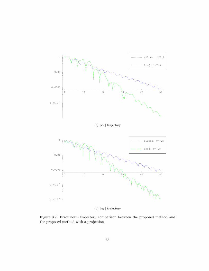
0 10 20 30 40 50

1. ´ 10-6

0.0001

0.01

1

Proj. Γ=7.5

Filter. Γ=7.5

(a) ‖e1‖ trajectory

0 10 20 30 40 50

1. ´ 10-8

1. ´ 10-6

0.0001

0.01

1

Proj. Γ=7.5

Filter. Γ=7.5

(b) ‖e2‖ trajectory

Figure 3.7: Error norm trajectory comparison between the proposed method andthe proposed method with a projection

55

10 20 30 40 50

3.6

3.8

4.2

4.4

4.6

4.8

Proj. Γ=7.5

Filter. Γ=7.5


10 20 30 40 50

0.2

0.4

0.6

0.8

1

1.2

Proj. Γ=7.5

Filter. Γ=7.5

(b) Parameter estimate trajectory for θ∗2

10 20 30 40 50

-0.5

-0.25

0.25

0.5

0.75

1

Proj. Γ=7.5

Filter. Γ=7.5

(c) Parameter estimate trajectory for θ∗3

Figure 3.8: Parameter estimates trajectory comparison according to the existenceof a projection mechanism 56

0 10 20 30 40

0.1

1

10 Proj. Γ=7.5

Filter. Γ=7.5


Figure 3.9: Control trajectory comparison according to the existence of a projectionmechanism

57

Chapter 4

Attitude Tracking Control

Problem with Unknown Inertia

Parameters

Following the previous chapter, the proposed control method is applied to the adap-

tive attitude tracking control problem. Since the attitude control system is nonlinear

in nature due to the kinematic relationship, it is natural to consider attitude control

problems as another application. Further, attitude control problems arise in various

fields of industries (e.g., spacecraft, unmanned aerial vehicle, unmanned marine ve-

hicle, etc.) and there have been a strong demand for the high performance control

scheme although several solutions exist. Thus, the new adaptive attitude control

scheme is designed to improve the overall system performance and demonstrated

through numerical simulations.

58

4.1 Introduction

The nonlinear control problem associated with spacecraft attitude dynamics has

been extensively studied and various proportional derivative (PD) type stabilizing

feedback solutions are currently available in the literature[32–35]. In particular,

the application of model reference adaptive control theory for stabilizing space-

craft attitude tracking dynamics in the presence of arbitrarily large inertia matrix

uncertainties has been largely enabled by the crucial fact that the governing dy-

namics permit affine representation of inertia related terms[36–38]. Nearly every

one of these existing adaptive attitude tracking control solutions are based upon

the classical certainty equivalence (CE) principle[10, 39] which permits the adaptive

controller to retain a structure that is identical to that of the deterministic case con-

troller wherein the inertia parameters are fully available (no uncertainty) except for

the introduction of an additional carefully designed parameter update (estimation)

mechanism that ensures stability with the adaptive controller and boundedness of

all resulting closed-loop signals.

In theoretical terms, the closed-loop error dynamics generated by CE-based

adaptive control solutions is exactly equivalent to the deterministic case control er-

ror dynamics whenever the estimated parameters coincide with their corresponding

unknown true values. Of course, this happens only when the underlying reference

trajectory satisfies suitable persistence of excitation (PE) conditions[39]. As a result,

typically, the control performance of CE-based adaptive attitude control methods

for either set-point regulation or trajectory tracking problems can at best match

the performance of the deterministic case controller, that too only when the PE

hypothesis ensure sufficiently fast convergence of parameter estimates to their true

values. However, in practice, the closed-loop performance obtained from CE-based

adaptive controllers is often seen to be arbitrarily poor when compared to the ideal

deterministic control case either due to non-satisfaction of PE conditions and/or

59

slow convergence rates for the parameter estimates. All these factors ultimately

reflect in terms of imposing wasteful rotational motion due to the control action

and thereby significant increases within the torque requirements and fuel costs.

This aforementioned performance degradation of CE-based adaptive con-

trol in attitude tracking/regulating problems is mainly caused by the fact that

search/estimation efforts of the parameter update law act like a additive distur-

bance imposed onto the deterministic case closed-loop dynamics. Another potential

cause of performance degradation is the fact that parameter estimation dynamics

are driven by the state regulation errors or tracking errors, which results in the

undesirable feature of parameter estimates being unable to get locked onto their

corresponding true values even if at any given instant during the estimation process

the estimates are equal to their true values. Moreover, parameter estimates from

CE-based adaptive control methods always deviate (drift) from their correspond-

ing true values even if they are initiated to exactly coincide with their true values

whenever there exists nonzero tracking/regulating error. Therefore, one may think

of improving the overall closed-loop performance of adaptive control schemes by ei-

ther eliminating in a stable fashion the disturbance type of terms within closed-loop

error dynamics arising due to estimation of uncertain parameters or by forcing the

parameter estimates stay locked at their true parameters once they are attained

during the estimation process. A technical challenge in this matter is to design such

a parameter update rule that would deal with both uncertain parameter effects and

estimation drift.

The main contribution is the introduction of a new non-certainty equivalence

(non-CE) adaptive attitude tracking control method that has potential to deliver

significantly superior closed-loop performance when compared to the classical CE-

based adaptive control schemes. Our results are partly motivated by the recently

formulated Immersion and Invariance (I&I) adaptive control theory[6, 9, 19]. The

60

I&I design is essentially a non-CE based adaptive control methodology that over-

comes many of the performance limitations arising from CE-based designs but ap-

plications of I&I adaptive control have thus far been somewhat limited to either

single-input nonlinear systems or linear multivariable systems. In this chapter, we

extend the I&I framework to the nonlinear spacecraft adaptive attitude tracking

problem endowed with three independent torque actuators. We are able to do so

while preserving all the key beneficial features of the I&I adaptive control methodol-

ogy by introducing a stable linear filter for the regressor matrix so that the parameter

adaptation dynamics reside within a stable and attracting manifold. In particular,

our novel controller design approach ensures that the additive disturbance type of

term arising within the closed-loop dynamics due to the parameter estimation error

decays to zero independent of satisfaction of any PE type conditions. Moreover,

rate of this decay can be prescribed to be arbitrarily fast while negligible or at worst

minimal impact on the overall fuel/control budgets. Yet another interesting and

important consequence of our new result that is never possible with existing CE-

based solutions is the fact that the proposed adaptive parameter estimation process

automatically stops if and when the parameter estimates happen to coincide with

their corresponding unknown true values. Our formulation is given in terms of the

globally valid (singularity-free) four-dimensional unit quaternion representation for

attitude. Assuming the spacecraft inertia matrix to be unknown, we make use of

full-state feedback, i.e., perfect measurement of body angular rate and the attitude

measurement in terms of the quaternion parameterization to guarantee globally sta-

ble closed-loop behavior with asymptotic convergence of regulation/tracking errors

for all possible initial conditions. It is pertinent here to observe the fact that the set

of special group of rotation matrices that describe body orientation in three dimen-

sions SO(3) is not a contractable space and hence quaternion based formulations

do not permit globally continuous stabilizing controllers[32, 33]. In this sense, we

61

adopt the standard terminology/notion of (almost) global stability for this problem

to imply stability over an open and dense set in SO(3) as is usually seen in literature

dealing with this problem[40]. It should also be emphasized that the basic approach

outlined in this chapter can be readily extended to other attitude representations

including minimal three-parameter sets[41–43].

This chapter is organized as follows. In section 4.2, the attitude tracking

control problem is formulated starting from basic description of quaternion kine-

matics and the Euler rotational dynamics equations. Then, in section 4.3, the main

theoretical results are presented along with detailed stability proofs. In section 4.5,

we show numerical simulation results for spacecraft attitude tracking control prob-

lems comparing our new non-CE method with a conventional CE-based method to

highlight the performance improvement due to presence of an attracting manifold

within the proposed parameter adaptation mechanism.


Euler’s rotational equations of motion state the rigid body attitude dynamics in

terms of its angular velocity ω(t) ∈ R3 prescribed in a body fixed frame, the mass

moment of inertia defined through the 3 × 3 symmetric positive-definite matrix J

(assumed to be an unknown constant), and an external control torque u(t) ∈ R3,

as follows

Jω(t) = −S(ω(t))Jω(t) + u(t) (4.1)

where the skew-symmetric matrix operator S(·) represents the vector cross product

operation between any two vectors as defined by

S(x)y = x× y; x,y ∈ R3 (4.2)

62

The corresponding kinematic differential equations governing the attitude motion

are given by

q(t) =12E(q(t))ω(t) (4.3)

where q(t) is the four-dimensional unit-norm constrained quaternion vector repre-

senting the attitude of the body-fixed frame FB with respect to the inertial frame

FN . In the following development, for the sake of notational simplicity, the time

argument ‘t’ is left out except at places where it is noted for emphasis. We de-

note qo and qv as scalar and vector parts of the unit quaternion respectively, i.e.,

q = [qo, qv]T along with the unit quaternion constraint qTq = 1. Quaternion oper-

ator E(q) in Eq. (4.3) is defined by

E(q) =

−qTv

qoI3×3 + S(qv)

(4.4)

where I3×3 is the 3×3 identity matrix. The direction cosine matrix can be obtained

from the quaternion vector through the following identity[34]

C(q) = I3×3 − 2qoS(qv) + 2S2(qv) (4.5)

and the time rate of change for the direction cosine matrix C(q) is given by the

well-known Poisson differential equation[34]

d

dtC(q) = −S(ω)C(q) (4.6)

which is the matrix version of the rotational kinematics stated through Eq. (4.3).

Since it is natural for the commanded angular velocity to be specified in its own

reference frame FR, we assume the commanded angular velocity ωr to be stated in

the reference frame FR and we denote qr to orient the commanded reference frame

63

FR with respect to the inertial frame FN . Then, the attitude and angular velocity

tracking errors are obtained as follows

C(δq) = C(q)CT (qr) (4.7)

δω = ω − C(δq)ωr (4.8)

where the attitude error quaternion δq = [δqo, δqv]T follows our notational conven-

tion. We note here that FB → FR means C(δq) → I3×3 (i.e., δq → [±1, 0, 0, 0]T ).

From the attitude error definition in Eq. (4.7), the attitude error dynamics is ob-

tained in a matrix form as follows

d

dtC(δq) = −S(ω)C(q)CT (qr) + C(q)CT (qr)S(ωr)

= −S(ω)C(δq) + C(δq)S(ωr)

= −S(ω)C(δq) + S(C(δq)ωr)C(δq)

= −S(ω − C(δq)ωr)C(δq)

=⇒ d

dtC(δq) = −S(δω)C(δq) ⇐⇒ δq =

12E(δq)δω (4.9)

wherein the identity C(δq)S(ωr) = S(C(δq)ωr)C(δq) has been employed which

can be easily proved by using the identity of the vector cross product under three

dimensional rigid rotation such that

C(δq)S(ωr)ν = C(δq)(ωr×ν) = C(δq)ωr×C(δq)ν = S(C(δq)ωr)C(δq)ν, ∀ν ∈ R3

(4.10)

Corresponding angular rate error dynamics for the rigid-body rotational motion is

given by differentiating Eq. (4.8) along Eq. (4.1) and Eq. (4.9). Thus, the overall

64

attitude tracking error dynamics are represented by

δq =12E(δq)δω (4.11)

Jδω = −S(ω)Jω + u+ J [S(δω)C(δq)ωr − C(δq)ωr] (4.12)

wherein the inertia matrix J is unknown and the adaptive control objective is to

determine control torque u(t) while employing full-state feedback [ω(t), q(t)] so as

to achieve boundedness of all closed-loop signals and convergence of tracking errors

limt→∞[δqv(t), δω(t)] = 0 for all possible reference trajectories [ωr(t), qr(t)] and

initial conditions [ω(0), q(0)]. We can summarize frames used in the analysis as

follows

FNq−−−−→ FB =⇒ b = C(q)n

FNqr−−−−→ FR =⇒ r = C(qr)n

FRδq−−−−→ FB

=⇒ b = C(δq)r (4.13)

where b, n, and r are the unit vector triads about FB, FN , and FR respectively.

4.3 Adaptive Attitude Tracking Control

In this section, we present a novel non-CE adaptive control method for the attitude

tracking problem represented by Eq. (4.11) and Eq. (4.12) while we specifically

focus on obtaining closed-loop performance improvement. The following theorem

represents the main results.

Theorem 4. Consider the attitude tracking error system Eq. (4.11) and Eq. (4.12)

with the inertia matrix J being unknown, and suppose the adaptive control input u

65

is determined through

u = −W (θ + β)− γWfW Tf [kp(ωf − δqv)− δω] (4.14)

˙θ = γW T

f [(α + kv)ωf + kpδqv]− γW Tωf (4.15)

β = −γW Tf ωf (4.16)

wherein kp, kv, γ > 0 are any scalar constants, α = kp + kv and the regressor ma-

trix W is constructed in the following fashion

Wθ∗ = −S(ω)Jω + J [S(δω)C(δq)ωC − C(δq)ωC ] + J (kvδω + kpδqv + αkpδqv)

(4.17)

where θ∗ = [J11, J12, J13, J22, J23, J33]T represents the elements of the unknown sym-

metric inertia matrix J = [Jij ]. Further, the signals Wf and ωf required in com-

puting the control input u in Eq. (4.14) are obtained from stable first-order linear

filter dynamics

ωf = −αωf + δω (4.18)

Wf = −αWf + W (4.19)

with arbitrary initial conditions Wf (0) ∈ R3×6 and ωf (0) ∈ R3. Then, for all

possible initial conditions [ω(0), q(0)] and reference trajectories [ωC(t), qC(t)],

the closed-loop is globally asymptotically stable leading to the convergence condition

limt→[δqv(t), δω(t)] = 0.

Proof. First, we re-arrange Eq. (4.12) into parameter affine form consistent with the

definition of the regressor matrix W in Eq. (4.17). Starting with the addition and

subtraction of terms J (kvδω + kpδqv + αkpδqv) to the right hand side of Eq. (4.12)

and following up through the regressor definition in Eq. (4.17) and some minor

66

algebraic manipulations, it is easy to obtain

δω = −kvδω − kp(δqv + αδqv) + J−1(Wθ∗ + u) (4.20)

where kv and kp are any scalar positive gains, and α = kv + kp as defined earlier

in this section. Obviously, the angular rate tracking error dynamics in Eq. (4.12)

is algebraically equivalent to Eq. (4.20) and accordingly, we shall henceforth refer

the overall attitude tracking error dynamics to be represented by Eq. (4.11) and

Eq. (4.20).

Next, we consider (only for purposes of the ensuing stability analysis) a linear

filter involving the control signal defined by

uf = −αuf + u (4.21)

so that we are able to work toward introducing a stable and attracting manifold into

the adaptation algorithm. Now, we transform the attitude tracking error dynamics

into the filtered attitude tracking error dynamics using Eq. (4.18) and Eq. (4.19).

Differentiating both sides of the filter dynamics in Eq. (4.18) followed by substitution

of the angular velocity error dynamics Eq. (4.20), it is easy to establish the following

perfect differential

d

dt

[ωf + kvωf + kpδqv − J−1(Wfθ

∗ + uf )]

=

− α[ωf + kvωf + kpδqv − J−1(Wfθ

∗ + uf )]

(4.22)

whose solution may be immediately established by

ωf = −kvωf − kpδqv + J−1 (Wfθ∗ + uf ) + εe−αt (4.23)

where the exponentially decaying term η(t) .= εe−αt on the right hand side of the

67

preceding equation is characterized by

η = −αη; η(0) = ε =[ωf (0) + kvωf (0) + kpδqv(0)− J−1 (Wf (0)θ∗ + uf (0))

](4.24)

We now suppose the filtered control signal uf be specified as follows

uf = −Wf

(θ + β

)(4.25)

in such a way that the composite term (θ+β) indicates an instantaneous estimate for

the unknown parameter vector θ∗ which therefore amounts to a significant departure

from the classical certainty equivalence adaptive control methodology. Accordingly

Eq. (4.23) becomes

ωf = −kvωf − kpδqv − J−1Wfz + εe−αt (4.26)

wherein the quantity z .= θ + β − θ∗ is introduced to indicate the parameter esti-

mation error. The dynamics of the parameter estimation error can be derived by

making use of Eq. (4.15), Eq. (4.16) and Eq. (4.26) to yield the following

z = ˙θ + β = −γW T

f J−1Wfz + γW Tf η (4.27)

Now, consider the lower bounded Lyapunov-like function given by

V =12ωT

f ωf + (δqo − 1)2 + δqTv δqv +

ζ

2λminzTz +

µ

2ηTη (4.28)

where λmin is the minimum eigenvalue of the unknown symmetric positive defi-

nite inertia matrix J , ζ > 9/(4γ) max [1/kv, 1/kp] and µ > 9/(4α) max [1/kv, 1/kp].

By taking the time derivative of V along trajectories generated from Eq. (4.11),

68

Eq. (4.15), Eq. (4.16), Eq. (4.24) and Eq. (4.26), we have the following

V = ωTf

(−kvωf − kpδqv − J−1Wfz + η

)+ δqT

v δω +ζ

λminzT ( ˙

θ + β)− µαηTη

= −kv‖ωf‖2 − kpωTf δqv − ωT

f J−1Wfz + ωTf η + δqT

v (ωf + αωf )−ζγ

λminzT W T

f J−1Wfz − µαηTη

= −kv‖ωf‖2 − kpωTf δqv − ωT

f J−1Wfz + ωTf η+

δqTv

(−kvωf − kpδqv − J−1Wfz + η + αωf

)− ζγ

λminzT W T


= −kv‖ωf‖2 − kp‖δqv‖2 − ωTf J−1Wfz + ωT

f η − δqTv J−1Wfz + δqT

v η−ζγ

λminzT W T


≤ −kv

3‖ωf‖2 −

kp

3‖δqv‖2 −

ζγ

3‖J−1Wfz‖2 −

µα

3‖η‖2−

kv

3

(‖ωf‖2 +

3kvωT

f J−1Wfz +ζγ

kv‖J−1Wfz‖2

)− kv

3

(‖ωf‖2 −

3kvωT

f η +µα

kv‖η‖2

)−

kp

3

(‖δqv‖2 +

3kp

δqTv J−1Wfz +

ζγ

kp‖J−1Wfz‖2

)− kp

3

(‖δqv‖2 −

3kp

δqTv η +

µα

kp‖η‖2

)≤ −kv

3‖ωf‖2 −

kp

3‖δqv‖2 −

ζγ

3‖J−1Wfz‖2 −

µα

3‖η‖2 (4.29)

which is negative semidefinite indicating boundedness for all closed-loop signals.

Further, since V is lower bounded and monotonic by the negative semidefinite-

ness of V , we know that∫∞0 V (t)dt exists and is finite, which, in turn, implies

ωf , δqv, J−1Wfz,η ∈ L2 ∩ L∞. This also implies boundedness of ωf , δqv, Wf ,

and z from Eq. (4.11), Eq. (4.15), Eq. (4.16), Eq. (4.19), and Eq. (4.26). By using

Barbalat’s lemma, we can now guarantee limt→∞[ωf (t), δqv(t), J−1Wf (t)z(t)] = 0.

Based on the last result, we may also show that limt→∞ ωf (t) = 0 from Eq. (4.26).

Finally, from Eq. (4.18), it follows that limt→∞ δω(t) = 0.

One last step remains now which is to recover the actual control input u

from the filtered control signal uf defined through Eq. (4.21) and Eq. (4.25). This

69

can be accomplished through

u = uf + αuf = −Wf (θ + β)−Wf

( ˙θ + β

)+ αuf (4.30)

By substituting Eq. (4.15), Eq. (4.16), and Eq. (4.19) in the preceding expression, the

adaptive control torque u can be recovered to be the expression given in Eq. (4.14),

thereby completing the proof of Theorem 4.

The following observations are now in order.

1. From positive definiteness of matrix J and the fact that we are able to prove

convergence condition limt→∞ J−1Wf (t)z(t) = 0, it follows that the proposed

adaptive controller provides for the establishment of an attracting manifold S

defined by

S =z ∈ R6 | Wfz = 0

(4.31)

in such a way that all closed-loop trajectories ultimately end up inside S.

Moreover, convergence to this attracting manifold can be made arbitrarily

fast by tuning the learning rate parameter γ present within the control law in

Eq. 4.14. This is a most significant feature of the non-CE adaptive controller

derived here given the fact that the term J−1Wf (t)z(t) essentially arises in

Eq. (4.26) due to the mismatch between current estimate of the parameter (θ+

β) and its corresponding true value θ∗ and therefore plays the role of being an

additive disturbance imposed onto the ideal case (no parameter uncertainty)

closed-loop system having dynamics given by

ωf = −kvωf − kpδqv + εe−αt (4.32)

A primary implication of this assertion is that the closed-loop performance

obtained in the ideal case is recovered through the presence of the attracting

70

manifold in the adaptive case; a feature that is seldom available with existing

CE-based adaptive control schemes. This statement can be further elaborated

based on the fact that conventional CE-based adaptive controllers rely upon

the cancelation of the uncertain parameter effects (within the time deriva-

tives of suitable Lyapunov-like candidate functions to render them negative

semi-definite), and accordingly the recovery of the ideal case (no uncertainty;

deterministic control) closed-loop performance happens only after either the

parameter estimates converge to their corresponding true values and/or the

tracking/regulating errors converge to zero. The role played by the learn-

ing rate parameter γ will be further illuminated in the numerical simulations

section.

2. The key steps that permit extension of the non-CE based I&I adaptive control

framework[6, 9] to the spacecraft adaptive attitude tracking control problem

are represented through our introduction of the regressor filter in Eq. (4.19)

and the algebraic developments leading to establishment of Eq. (4.20) which

were made possible by judiciously adding and subtracting the following term

J (kvδω + kpδqv + αkpδqv)

to the right hand side of Eq. (4.12). Also important to note is the fact that

only the angular rate error signal δω needs to be filtered through Eq. (4.18)

to obtain the signal ωf which is required for the controller implementation

whereas no filtering is needed on the attitude error signal represented by the

unit-norm constrained error quaternion δq. Moreover, in the non-adaptive

ideal case, if the parameter θ∗ is exactly known (no uncertainty), then the

filtered control signal specified in Eq. (4.25) can be replaced by simply using

uf = −Wfθ∗ ultimately leading to u = αuf + uf = −Wθ∗ thereby obviating

71

any need for the regressor filter of Eq. (4.19) during controller implementation.

3. It is always possible to introduce the filter states such that η(t) = 0 for all

t ≥ 0 by letting η(0) = 0 based on the suitable selection of initial filter states

such as ωf (0) = (δω(0)+kpδqv(0))/kp and Wf (0) = 0 in Eq. (4.26). This will

further improve the transient performance of the closed-loop adaptive attitude

control system because η(t) = 0 eliminates the time and control effort needed

toward enabling the filter state convergence. Of course, as seen from the

preceding proof, even in the case that η(0) 6= 0, closed-loop stability and

overall convergence of the trajectories to the attracting manifold S remains

true and the signal η(t) still converges to zero exponentially fast. However,

having η(0) = 0 permits us rewrite the dynamics governing the parameter

estimation error signal z given in Eq. (4.27) as follows

z = −γW Tf J−1Wfz (4.33)

which is rigorously linear with respect to the parameter estimation error z.

Thus, if at any instant of time t, the parameter estimation error z is equal to

zero, then adaptation stops henceforth and thereby parameter estimates stay

locked at their true values (i.e., if z(t∗) = 0 for some t∗ > 0, then z(t) = 0 for

all t ≥ t∗). We emphasize here that this nice feature is available only if the

filter initial conditions are chosen such that η(0) = 0 and such a possibility is

never available with existing CE-based formulations.

4. Finally, one needs to be extra careful while interpreting the properties of

the attracting manifold definition S defined in Eq. (4.31) to the extent that

limt→∞ z(t) = 0 obviously implies limt→∞Wf (t)z(t) = 0 but the converse is

not necessarily true. Therefore, just as with CE-based controllers, even under

the proposed non-CE adaptive control scheme, there is no recourse from en-

72

suring satisfaction of suitable PE conditions on the reference trajectory if one

were interested in ensuring convergence of all the parameter estimates to their

respective unknown true values.

4.4 Adaptive Control with Parameter Projection

In Chapter 3, we use a projection technique wherein the unknown parameters are

positive real. Here, we assume that the bounds for each element of the inertia

matrix are given as a priori (i.e., θk ∈ (θmin, θmax) for k = 1, . . . , 6). Then, from

the definition of θ∗ in Eq. (4.17), the necessary reparameterization θ∗p is given as

follows:

θ∗p =

δ1(tanh φ∗1 + 1) + θ∗1min


...


(4.34)

θp(t) =

δ1(tanh(φ1(t) + β1(t)) + 1) + θ∗1min

δ2(tanh(φ2(t) + β2(t)) + 1) + θ∗2min

...

δ6(tanh(φ6(t) + β6(t)) + 1) + θ∗6min

(4.35)

where δk = (θ∗kmax− θ∗kmin

)/2 for k = 1, . . . , 6. We see in Eq. (4.35) that each

element of θp remains within the a priori bounds of θ∗p by definition. Based on

the reparameterization in Eq. (4.34) and Eq. (4.35), the stability of the proposed

attitude control method combined with the smooth projection technique is presented

in the followings.

Theorem 5 (Adaptive Attitude Tracking Control with Projection). For the attitude

tracking system represented by the error dynamics Eq. (4.11) and Eq. (4.12), let the

73

control torque u computed by

u = −W θp − γWfDiag[κ]W Tf ((kv − α)ωf + kpδqv + δω) (4.36)

wherein φ and β is computed by

˙φ(t) = γ(αWf −W )Tωf + γW T

f (kvωf + kpδqv) (4.37)

β = γW Tf ωf (4.38)

In addition, Diag[·] is defined in Eq. (3.27) and

κ =

δ1sech2(φ1 + β1)

δ2sech2(φ2 + β2)...

δ6sech2(φ6 + β6)

(4.39)

kp, kv, γ, and α are defined in Theorem 4. Filters and regressor matrix W are

identical to Eq. (4.18), Eq. (4.19), and Eq. (4.17) respectively. Then, the atti-

tude tracking control objective is satisfied, i.e., limt→∞[δqv(t), δω(t)] = 0 for all

[δqv(0), δω(0)] ∈ R6.

Proof. Starting from Eq. (4.20), filtered error dynamics for ωf are obtained by

substituting filter states Eq. (4.18), Eq. (4.19), and Eq. (2.8) along with uf =

−Wf θp as follows

ωf = −kvωf − kpδqv − J−1Wfχ (4.40)

where we use the same definitions for a parameter estimation error χ and adaptation

discrepancy z as in Eq. (3.28) and Eq. (3.29). More specifically, χ is expressed as

follows

χk = δk

[tanh(φk + βk)− tanh φ∗k

](4.41)

74

Then, consider the following Lyapunov candidate function Vp given by

Vp =12ωT

f ωf + (δq0 − 1)2 + δqTv δqv+

ζ

2λmin

6∑k=1

δk [log cosh(zk + φ∗k)− zk tanh φ∗k]︸︷︷︸P

(4.42)

which is an identical definition of Eq. (4.28) except for P function and missing η

term (we ignored η because it plays no role on the stability proof as already shown

in the previous section). In a similar way in the projection section in Chap. 3, we

can prove that P is a lower bounded and monotonically increasing function with

respect to ‖z‖ by the followings:

P ′zk= δk

∂

∂zk(log cosh(zk + φ∗k)− zk tanh φ∗k)

= δk (tanh(zk + φ∗k)− tanh φ∗k)

> 0 if zk > 0

< 0 if zk < 0

= 0 at zk = 0

(4.43)

P ′′zk= δk

∂

∂zk(tanh(zk + φ∗k)− tanh φ∗k) = δksech2(zk + φ∗k) > 0 for all zk (4.44)

Thus, Vp is lower bounded and positive with respect to [ωf , δqv,z]. Next, by taking

time derivative of Vp in Eq. (4.42) and substituting Eq. (4.40), Eq. (4.11), Eq. (4.37),

75

and Eq. (4.38), we obtain the result

Vp =ωTf

(−kvωf − kpδqv − J−1Wfχ

)+ δqT

v (ωf + αωf ) +

ζ

λmin

6∑k=1

δk [tanh(zk + φ∗k)− zk tanh φ∗k] (˙φk + βk)︸︷︷︸

χT z

=− kvωTf ωf − kpδq

Tv δqv − ωT

f J−1Wfχ− δqTv J−1Wfχ−

ζγ

λminχT W T

f J−1Wfχ

6− kv

2‖ωf‖2 −

kp

2‖δqv‖2 −

ζγ

3‖J−1Wfχ‖2

− kv

2

(‖ωf‖2 −

2kv‖ωf‖‖J−1Wfχ‖+

2ζγ

3kv‖J−1Wfχ‖2

)− kp

2

(‖δqv‖2 −

2kp‖δqv‖‖J−1Wfχ‖+

2ζγ

3kp‖J−1Wfχ‖2

)6− kv

2‖ωf‖2 −

kp

2‖δqv‖2 −

ζγ

3‖J−1Wfχ‖2 (4.45)

Because the foregoing inequality result is the same as Eq. (4.29) except that z is

replaced by χ and η is ignored, we can argue the similar signal chasing process and

thereby it is guaranteed that limt→∞[δqv, δω] = 0. u is obtained from u = uf +αuf

following the same steps described in Eq. (3.37).

Attracting manifold is defined by SAP as follows

SAP = χ | Wfχ = 0 (4.46)

As in the robot application with projection algorithm, χ has the estimation error

property of z in Eq. (4.31).

76


4.5.1 Proposed Control without Projection Mechanism

In order to demonstrate the various features of the proposed adaptive attitude con-

trol method, we perform numerical simulations and compare the closed-loop tra-

jectory tracking simulation results with the quaternion CE-based adaptive control

results from Ref. [38]. Two sets of simulations are performed. In the first case, the

reference trajectory does not satisfy the underlying persistence of excitation con-

ditions to ensure convergence of parameter estimates to their corresponding true

unknown values. The second set of simulations consider a persistently exciting ref-

erence trajectory.

The numerical model for the attitude tracking control system has the follow-

ing system parameters. The unknown inertia matrix is described by

J =

20 1.2 0.9

1.2 17 1.4

0.9 1.4 15

(4.47)

which can be rewritten as in vector form as θ∗ = [20, 1.2, 0.9, 17, 1.4, 15]T . The

corresponding CE-based adaptive control law taken from Ref. [38] is listed below

uce = 2(P−1)T

[−Y θce −Kr − δqv

1− δqTv δqv

](4.48)

˙θce = ΓY Tr (4.49)

where r .= δqv + αceδqv; P.= δqoI3×3 + S(δqv) corresponds to the vector part

operator of E(q) in Eq. (4.4); Y ∈ R3×6 is a regressor matrix corresponding our W

in Eq. (4.17); αce,K ∈ R3×3 are constant, positive definite, diagonal gain matrices;

and Γ ∈ R6×6 is any learning rate matrix that is also constant, positive definite, and

77

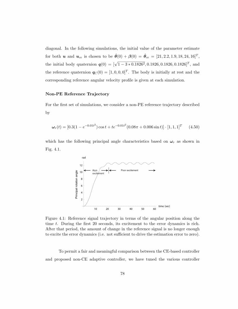
diagonal. In the following simulations, the initial value of the parameter estimate

for both u and uce is chosen to be θ(0) + β(0) = θce = [21, 2.2, 1.9, 18, 24, 16]T ,

the initial body quaternion q(0) = [√

1− 3 ∗ 0.18262, 0.1826, 0.1826, 0.1826]T , and

the reference quaternion qC(0) = [1, 0, 0, 0]T . The body is initially at rest and the

corresponding reference angular velocity profile is given at each simulation.

Non-PE Reference Trajectory

For the first set of simulations, we consider a non-PE reference trajectory described

by

ωr(t) = [0.3(1− e−0.01t2) cos t + te−0.01t2(0.08π + 0.006 sin t)] · [1, 1, 1]T (4.50)

which has the following principal angle characteristics based on ωr as shown in

Fig. 4.1.

10 20 30 40 50 60time (sec)

2

4

6

8

10

12

rad

Figure 4.1: Reference signal trajectory in terms of the angular position along thetime t. During the first 20 seconds, its excitement to the error dynamics is rich.After that period, the amount of change in the reference signal is no longer enoughto excite the error dynamics (i.e. not sufficient to drive the estimation error to zero).

To permit a fair and meaningful comparison between the CE-based controller

and proposed non-CE adaptive controller, we have tuned the various controller

78

parameters to obtain similar error convergence rates as shown in Fig. 4.2 assuming

that the inertia matrix J is known (ideal case performance).

The corresponding control gains are determined as follows: αce = diag10, 10, 10,

K = diag10, 10, 10, Γ = diag0.1, 0.1, 0.1, 0.1, 0.1, 0.1 for the CE-based method;

and kv = 0.5, kp = 0.5, γ = 100 for the proposed method. The wriggle seen in

Fig. 4.2 for the proposed method is from the fact that the deterministic/ideal case

error dynamics (described by Eq. (4.26) with Wfz = 0) correspond to a second-order

system whereas the ideal case closed-loop dynamics under the CE-based method re-

sult in a stable first-order system in terms of the composite error signal r (for further

details, refer [38]).

Next, we assume the inertia matrix J to be unknown and simulate both

the CE and non-CE adaptive controllers. The resulting closed-loop simulations are

documented in Fig. 4.3. Initial filter state values for the proposed method are cho-

sen as follows: Wf (0) = 0 and ωf (0) = (δω(0) + kpδqv(0))/kp, thereby satisfying

η(t) = 0 for all t ≥ 0. The learning rate Γ of the CE-based adaptive control

method in Eq. (4.49) and its counterpart γ for the proposed adaptive controller

are systematically tuned to achieve performance that is as close as possible as the

ideal case performance obtained for both methods in Fig. 4.2. The attitude and

angular rate errors converge to zero with both adaptive controllers. However, as

seen in Fig. 4.3(a) and Fig. 4.3(b), the closed-loop performance from the proposed

method remains more or less the same when compared to the corresponding ideal

case performance in Fig. 4.2. This is clearly not the case with the CE-based con-

troller because the attitude and angular rate errors exhibit a very slow convergence

trend in Fig. 4.3. The norms of the control torques commanded by the CE-based

controller and the non-CE controller are both plotted in Fig. 4.3(c) where it can

be clearly seen that the torque demands due to the CE-based adaptive controller

are severe during the initial transient. Given that we are simulating a trajectory

79

0 10 20 30 40 50 60

1. ´ 10-12

1. ´ 10-9

1. ´ 10-6

0.001

1

C.E.

Proposed

(a) quaternion error δqv

0 10 20 30 40 50 60

1. ´ 10-10

1. ´ 10-7

0.0001

0.1C.E.

Proposed

(b) angular velocity error δω

Figure 4.2: Ideal case closed-loop performance obtained with the CE-based and theproposed non-CE controller assuming the inertia matrix J to be known

80

0 10 20 30 40 50 60

1. ´ 10-12

1. ´ 10-9

1. ´ 10-6

0.001

1 C.E.

Proposed


0 10 20 30 40 50 60

1. ´ 10-12

1. ´ 10-9

1. ´ 10-6

0.001

1 C.E.

Proposed


81

0.00001 0.001 0.1 10

0

5

10

15

20

25

30

35

C.E.

Proposed

(c) initial transient of control norm highlighting the difference between CE-based and theproposed adaptive control methods

0 10 20 30 40 50 60

0.75

1

1.25

1.5

1.75

2

2.25

C.E.

Proposed

(d) parameter estimation error norm

Figure 4.3: Adaptive attitude tracking closed-loop performance comparison betweenthe classical CE-based controller and the proposed non-CE controller for a non-PEreference trajectory

82

tracking problem, the steady state torques obviously remain time-varying to ensure

tracking along the prescribed reference trajectory. The parameter estimation er-

ror norms are compared in Fig. 4.3(d). We recognize that parameter estimation

error fails to converge to zero for both methods due to the non-PE nature of the

underlying reference trajectory.

The role played by the parameter γ in the proposed adaptive controller is

studied next. It is clear from Eq. (4.27) that whenever η(0) = 0, the attractiveness of

manifold S can be accelerated by increasing the value of γ parameter. This implies

the ideal case (no uncertainty) closed-loop performance can be closely recovered

with increasing γ values. We consider two different γ values: γ = 10 and γ = 100

and report the simulation results in Fig. 4.4. For the larger γ case, the attitude

tracking performance is improved as seen from the faster attitude and angular rate

error convergence in Fig. 4.4(a) and Fig. 4.4(b). Parameter estimation error with

large γ also converges faster than one with small γ in Fig. 4.4(d) since the manifold

attractivity of Eq. (6.27) is increased. In Fig. 4.4(c), we recognize that the peak

control norm is mostly unchanged in spite of the increased γ value since the reduction

in the parameter estimation error due to the larger γ value contributes to a decrease

in the control norm during the transient part of the simulation.

83

0 10 20 30 40 50 60

1. ´ 10-9

1. ´ 10-6

0.001

1

1000

Γ=10

Γ=100


0 10 20 30 40 50 60

1. ´ 10-9

1. ´ 10-6

0.001

1

1000

Γ=10

Γ=100


84

0 10 20 30 40 50 60

2

4

6

8

10

12

14

16

Γ=10

Γ=100

(c) Control norm

0 10 20 30 40 50 600.75

1

1.25

1.5

1.75

2

2.25

Γ=10

Γ=100


Figure 4.4: Performance study of the proposed non-CE adaptive attitude trackingcontroller for two different different γ values

85

PE Reference Trajectory

We now consider the case wherein the reference trajectory is persistently exciting so

that parameter estimates from the CE-based controller and the proposed non-CE

controller may converge to their corresponding true values. The reference angu-

lar velocity for this simulation is taken to be ωrp(t) = [cos t + 2, 5 cos t, sin t + 2]T .

Before comparing the closed-loop performance of each method, we first tune the de-

terministic (ideal case non-adaptive) control performance as done before in Fig. 4.5,

which leads to αce = 8 (the rest of control gains are same as before). The inertia

matrix is once again assumed unknown and the adaptive control simulations for the

PE reference trajectory case are shown in Fig. 4.6. First, we note that the attitude

and angular rate error convergence remains slow with the CE-based method. Since

the reference trajectory is persistently exciting, the parameter estimates converge

to their true values and this convergence rate is significantly faster for the proposed

method compared to the CE-based approach as seen in Fig. 4.6(d).

86

0 10 20 30 40 50 60 701. ´ 10-13

1. ´ 10-10

1. ´ 10-7

0.0001

0.1

C.E.

Proposed

(a) quaternion tracking error δqv

0 10 20 30 40 50 60 701. ´ 10-13

1. ´ 10-10

1. ´ 10-7

0.0001

0.1

C.E.

Proposed


Figure 4.5: Ideal case closed-loop performance for the PE reference trajectory ob-tained with the CE-based and the proposed non-CE controller assuming the inertiamatrix J to be known

87

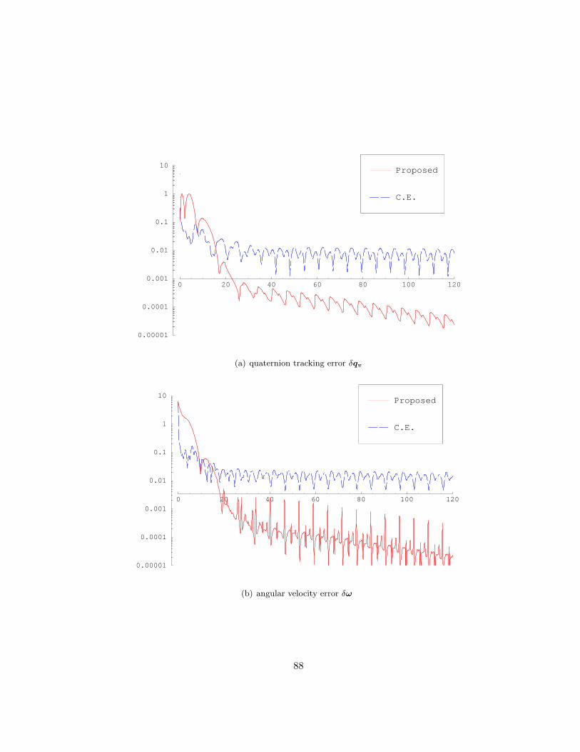
0 20 40 60 80 100 120

0.00001

0.0001

0.001

0.01

0.1

1

10

C.E.

Proposed

(a) quaternion tracking error δqv

0 20 40 60 80 100 120

0.00001

0.0001

0.001

0.01

0.1

1

10

C.E.

Proposed


88

0.00001 0.001 0.1 10

0

250

500

750

1000

1250

1500

C.E.

Proposed

(c) control norm

0 20 40 60 80 100 120

0.5

1

1.5

2

2.5

C.E.

Proposed


Figure 4.6: Adaptive attitude tracking closed-loop performance comparison betweenthe classical CE-based controller and the proposed non-CE controller for a PE ref-erence trajectory

89

4.5.2 Proposed Control with Projection Mechanism

In the following simulation where the proposed control scheme is combined with the

projection algorithm, system response trajectories are compared with those of the

foregoing adaptive controller. γ is set to 20 during the simulation and the reference

attitude trajectory is generated by ωr(t) in the previous section. In addition, system

parameters of Eq. (4.47) are used. The performance of the proposed controller with

projection is better than that of the proposed controller only. Although the transient

response of both control methods are comparable during first 20 seconds, we notice

in Fig. 4.7 that the proposed controller with projection shows a smaller error-norm

trajectory in the long run. One thing needs to be mentioned here is that this

simulation is performed with a relatively small γ value. If we increase γ value,

then the trajectories of both closed-loop systems converge to the ideal trajectory

(deterministic case of the proposed controller) shown in Fig. 4.2. Differences are

highlighted in Fig. 4.8. The estimation trajectories of the proposed control method

with projection do not leave known parameter bounds (denoted by brown lines)

while some of the proposed control method without projection cross the parameter

bound line. Lastly, we see that parameter estimates of both methods fail to identify

true parameter values because of the non-persistence excitation of the reference

signal ωr.

90

0 20 40 60 80 100t

0.001

0.01

0.1

þ ∆qv þ

Projection Γ=20

Filter Γ=20

(a) Quaternion error norm trajectory

0 20 40 60 80 100t

1. ´ 10-6

0.00001

0.0001

0.001

0.01

0.1

1

þ ∆Ωþ

Projection Γ=20

Filter Γ=20

(b) Angular velocity error norm trajectory

Figure 4.7: Error norm trajectory comparison between the proposed method andthe proposed method with a projection

91

20 40 60 80 100t

17.5

20

22.5

25

27.5

30

32.5

35

Upper & Lower

True

Projection Γ=20

Filter Γ=20


20 40 60 80 100t

0

2

4

6

Upper & Lower

True

Projection Γ=20

Filter Γ=20

(b) Parameter estimate trajectory for θ∗2

20 40 60 80 100t

0

2

4

6

Upper & Lower

True

Projection Γ=20

Filter Γ=20

(c) Parameter estimate trajectory for θ∗3

92

20 40 60 80 100t

16

18

20

22

24

26

28

30

Upper & Lower

True

Projection Γ=20

Filter Γ=20

(d) Parameter estimate trajectory for θ∗1

20 40 60 80 100t

0

2

4

6

Upper & Lower

True

Projection Γ=20

Filter Γ=20

(e) Parameter estimate trajectory for θ∗2

20 40 60 80 100t

12.5

15

17.5

20

22.5

25

27.5

Upper & Lower

True

Projection Γ=20

Filter Γ=20

(f) Parameter estimate trajectory for θ∗3

Figure 4.8: Parameter estimates trajectory comparison according to the existenceof a projection mechanism

93

Chapter 5

Attitude Estimator with Known

Angular Velocity

This chapter includes an overview of the attitude estimation problem and presents

an novel approach to it by designing an attracting manifold. The designed attracting

manifold through an adaptive estimation update preserves the orthogonal structure

of attitude matrices on all n-dimensional spaces. In Chapter 6, the developed atti-

tude estimator is combined with the proposed adaptive attitude tracking controller

to be implemented in real systems.

5.1 Introduction

Attitude estimation problems arising in numerous aerospace and robotics applica-

tions are about how to find a 3-dimensional attitude matrix from an input-output

relationship. The attitude matrix is represented by a proper orthogonal matrix

in SO(3) topologically. Thus, the actual unknown element number is 6 although

the total number of elements in the attitude matrix is 9. Based on this property,

numerous attitude estimation/determination algorithms are available in the liter-

94

ature presented by both control and estimation communities. The important fact

is that conventional estimation methods rely on linear over-parameterization of 6

elements[44] although 6 elements are nonlinear parameterization of fewer number of

coordinates[42, 45]. In addition to grouping conventional estimation methods based

on attitude parameterization, depending on how the underlying attitude estimation

algorithm is implemented, we may also categorize them broadly into two classes:

batch type and sequential type estimators.

Batch type estimators utilize more than two observations at each observa-

tion instant to determine the attitude matrix, thereby necessitating the use of two

or more independent sensors. QUEST[46] and FOAM[47] belong to the class of

batch type estimators. Estimates of attitude matrix are computed by minimizing a

quadratic cost function originally proposed by Wahba[48] in a statistical way. An-

other variant of batch estimator in use is TRIAD[49], which requires at most n − 1

linearly independent observation vectors for n-dimensional attitude matrices to solve

a matrix equation deterministically[50].

Sequential type estimators, in contrast with batch type estimators, need only

one observation at each observation instant. An extended Kalman filter[51] is one

of most commonly used sequential type estimators. Instead of fusing measurements

from multiple sensors at each instant, sequential type estimators utilize an analytic

model of the system to forward propagate the observation data. Attitude estimates

are then generated by comparing predicted observations with actual measurements

while updating the underlying analytic model through minimization of a suitable

optimality criterion. The standardly adopted optimality criterion for Kalman fil-

tering is the minimization of variances between estimates from sensor measurement

and predicted values derived from the system analytic model. Applications of ex-

tended Kalman filter type sequential estimators are documented for missions such

as the Earth Radiation Budget Satellite (ERBS)[52, 53] and the Solar Anomalous

95

Magnetospheric Particle Explorer (SAMPEX)[54, 55].

Both batch and sequential type estimators have successfully found their ap-

plication in a wide array of spacecraft missions. However, they usually have a crucial

limitation due to the over-parameterization and resulting non-orthogonal attitude

estimates. In order to eliminate problems associated with over-parameterization,

recently, an adaptive algorithm for orthogonal matrix estimation was developed by

Kinsey and Whitcomb[56]. The convergence proof for their algorithm utilizes a

matrix logarithmic map defined over the attitude estimation in the 3-dimensional

space, which means the extension to n-dimensional space requires a n-dimensional

matrix logarithmic map. Further, the matrix logarithmic map is not injective for

certain class of orthogonal matrices. Precisely stated, SO(3) group, where attitude

matrices belong, does not include the orthogonal matrix whose trace is −1 (the

corresponding Euler principal rotation angle φ = ±π).

In this chapter, we present new classes of adaptive estimation algorithms for

uncertain n×n proper orthogonal matrices. The proposed estimation methodology

introduces an attracting manifold about the “true” but “unknown” attitude ma-

trix where estimate and true attitude matrices become identical under a standard

observation condition. Simultaneously, the attracting manifold helps enforcing the

attitude matrix estimate to be proper and orthogonal at every time step. Design

of the attracting manifold results in significant reduction of computational burden

associated with: (a) being able to fully utilize the available prior information on

orthogonality of the unknown attitude and thereby avoiding over-parameterization;

and (b) not having to perform the re-orthogonalization process at each time step.

The standard observation assumption refer to the availability of persistence in ex-

citation (PE) and we are able to show that the attitude estimate is guaranteed to

converge to the corresponding true value with PE condition. Convergence proof for

the proposed estimation algorithm is accomplished in such a way that not only are

96

the restrictions associated with the logarithmic map of Kinsey and Whitcomb[56]

are completely eliminated but our results also generalize nicely for attitude matrices

on all n-dimensional spaces.

This chapter is organized as follows. In the following section, adaptive atti-

tude estimation problems are formulated under standard assumptions such as known

reference signal, bounded noise, and persistent excitation. Then, we present main

results that establish a new orthogonality preserving attitude matrix estimation

algorithm valid for the general n-dimensional case. In section 5.3.2, robustness

analysis for the proposed estimation algorithm subject to the measurement noise

is presented. Implications of the developed estimation algorithm for 2-dimensions

followed by 3 dimensions are discussed in section 5.4 and 5.5 respectively. Numer-

ical simulation results are presented in section 5.6 to demonstrate and validate the

proposed algorithm.


As mentioned before, adaptive attitude estimation method depends on the contin-

uous time input-output attitude equation represented as follows

y(t) = C(t)r(t) (5.1)

where C(t) is an unknown time-varying proper orthogonal matrix; i.e., a time-

varying direction cosine matrix satisfying C(t)CT (t) = CT (t)C(t) = In×n and

det(C(t)) = 1 for all t. Unit vectors r(t) ∈ Rn and y(t) ∈ Rn respectively cor-

respond to the input and output signals, both of which are assumed accessible for

all time t. In addition, r(t) is assumed to be a differentiable function of time with

a bounded derivative. The measurement model Eq. (5.1) is from a model of mea-

surement sensors such as star trackers, sun sensors and magnetometers[57]. More

97

specific examples of star sensor modeling in attitude determination problems can be

found in [58, 59]. For the magnetometer and its modeling, refer to [60]. In general, a

few sensors are equipped together to achieve high accurate attitude information[61].

C(t) evolves along the time t by the following Poisson differential equation

C(t) = −S(ω(t))C(t) (5.2)

where ω(t) ∈ Rm is any prescribed/measured bounded signal for m = n(n − 1)/2,

and S(·) : Rm → Rn×n is a skew-symmetric matrix function such that ST = −S.

The fact is that if C(0) is a proper orthogonal matrix, then C(t) is always a proper

and orthogonal matrix for all t whenever it evolves along Eq. (5.2)[62]. The esti-

mation objective is to find an adaptive algorithm computing the proper orthogonal

matrix C(t) ∈ Rn×n as an estimate for the “true” but unknown matrix C(t) at each

instant t. Since C(t) is orthogonal, the estimator structure is the same as Eq. (5.1)

and represented as

y(t) = C(t)r(t). (5.3)

Analogous discrete-time estimator structure with different update laws for C(t) can

be found in the spacecraft attitude determination problems. In such cases, r(t)

and y(t) are respectively interpreted as the star catalog values (inertial) and the

corresponding star tracker measurements. Spacecraft rendezvous and proximity op-

erations computing relative navigation solutions are other examples for the proposed

adaptive attitude estimation framework. To quantify the error between the true at-

titude matrix and its estimate, the attitude estimation error matrix C(t) is defined

by matrix subtraction as follows

C(t) = C(t)− C(t) (5.4)

98

Obvious from the definitions in Eq. (5.1) and Eq. (5.3) is the fact that the at-

titude error convergence, limt→∞ C(t) = 0, implies the output estimation error,

e(t) .= y(t) − y(t) → 0 as t → ∞. In the following developments, unless consid-

ered necessary, the time argument t is omitted from various signals for the sake of

notational simplicity.

5.3 Adaptive Attitude Estimation with Attracting Man-

ifold

In this section, we present an adaptive estimate update law for C(t), its robustness

analysis subject to bounded measurement noise, and comparison with certainty

equivalence principle.

5.3.1 Main Result

Theorem 6. If the attitude estimate C(t) is generated by

˙C(t) = −

[S(ω)− γ(yyT − yyT )

]C(t);

any real γ > 0, any proper orthogonal C(0) ∈ Rn×n (5.5)

then, C(t) remains a proper orthogonal matrix for all t > 0 implying that attitude

matrix estimation error C(t) and the output estimation error e(t) remain bounded

for all t ≥ 0. In addition, the estimation process for C(t) is driven along an “at-

tracting manifold” according to the following convergence condition

limt→∞

(In×n − CT CCT C

)r(t) = 0. (5.6)

Proof. Like the Poisson differential equation Eq. (5.2) preserving orthogonality of

C(t) for all t, Eq. (5.5) enforces orthogonality of C(t) for all t. This is simply because

99

(yyT − yyT ) is also a skew-symmetric matrix. Thus, C(t) and C(t) remain bounded

for all t, which means e(t) is also bounded for all t. The convergence property along

the attracting manifold of Eq. (5.6) is proved by considering the following Lyapunov

candidate function

V (t) =12tr(CT (t)C(t)) (5.7)

where tr(·) is the matrix trace operator. Taking the time derivative of V (t) in

Eq. (5.7) along the update dynamics Eq. (5.5) leads to the following equality

V (t) = tr(−CT S(ω)C + γCT (yyT − yyT )C

)= γtr

(CT (yyT − yyT )C

)= γtr

((CT − CT )(CrrT − CrrT CT C)

)= γtr

(−rrT + CT CCT CrrT

)= −γrT (In×n − CT CCT C)r

= −γ

2rT (In×n − CT CCT C − CT CCT C + In×n)r

= −γ

2rT (In×n − CT CCT C − CT CCT C + (CT CCT C)T (CT CCT C))r

= −γ

2rT (In×n − CT CCT C)T (In×n − CT CCT C)r

= −γ

2‖(In×n − CT CCT C)r‖2 (5.8)

Since V (t) ≥ 0 from Eq. (5.7) and V (t) ≤ 0 from Eq. (5.8), we have existence of

V∞.= limt→∞ V (t). Moreover, from the fact that V (t) is bounded (seen by differen-

tiating both sides of Eq. (5.8)), using Barbalat’s lemma, we conclude limt→∞(In×n−

CT CCT C)r(t) = 0.

Remark 5. From the definition of C(t) in Eq. (5.4), we see that the convergence of

C(t) to C(t) leads to limt→∞ C(t) = 0, which is equivalent to CT (t)C(t) → In×n

as t → ∞ by the matrix orthogonality property. This means the satisfaction of

100

the convergence condition of Theorem 6 in Eq. (5.6). However, the inverse of the

pervious statement is not true. In general, the satisfaction of Eq. (5.6) does not

guarantee the convergence of C(t) to C(t) without certain persistence of excitation

(PE) conditions for r(t). These PE conditions will be further elaborated upon in

the later sections.

5.3.2 Robustness Analysis

In order to account for the effect of measurement noise, the input-output attitude

equation is modified as follows

y(t) = C(t)r(t) + v(t) (5.9)

where measurement noise v(t) is assumed to be bounded and its bound is vmax.=

supt‖v(t)‖. In addition, from a practical standpoint, we may assume that vmax 1

without loss of generality though this assumption is not required for our analysis.

With the same estimation update rule for C(t) as in Eq. (5.5), consider the following

Lyapunov candidate function

Vr(t) =12tr[CT C

]. (5.10)

Because of the same estimation update law for C(t), proper orthogonality of C(t) is

preserved regardless of measurement noise v(t). Thus, Vr(t) is uniformly bounded.

Further, the time derivative of Vr(t) is obtained using Eq. (5.3), Eq. (5.5), and

101

Eq. (5.9) as follows

Vr(t) = tr(C

˙C)

= γtr(CT (yyT − yyT )C

)= −γrT

(I − CT CCT C

)r − γvT C

(I − CT CCT C

)r

6 −γ

2‖(In×n − CT CCT C)r‖

[‖(In×n − CT CCT C)r‖ − 2vmax

]. (5.11)

By the presence of measurement noise v(t), the sign indefinite term γvT C(I − CT CCT C

)r

is introduced; thus, the convergence property of Eq. (5.6) is no longer valid. How-

ever, we may conclude that the residual set of Vr(t) is governed by vmax based on

the fact that Vr(t) ≤ 0 in Eq. (5.11) whenever ‖(In×n − CT CCT C)r‖ − 2vmax ≥ 0.

The foregoing robustness analysis of the proposed estimation algorithm confirms

that while all the signals remain bounded, accuracy of estimated attitude values is

deteriorated by measurement noise.

5.3.3 Comparison with Certainty Equivalence Framework

In this section, the proposed adaptive estimation algorithm in Theorem 6 and the

conventional adaptive estimation algorithm based on certainty equivalence principle

(CE)[39] are compared to explore the difference between them. In order to be con-

sistent with the standard assumptions of the CE methodology, C(t) is restricted to

be a constant C∗ (i.e., ω(t) = 0 in Eq. (5.2)). Benefits of the proposed estimation

algorithm is originated from the fact that it preserves the proper and orthogonal

structure of estimate C(t) along time t, while the conventional adaptive estima-

tion schemes cannot. The reason for the foregoing fundamental difference is how

to parameterize the unknown C∗. Utilizing the orthogonal structure of C∗ as prior

information results in the nonlinear parameterization of C∗ in Eq. (5.1), which is

not readily amenable to most existing CE-based formulations. On the other hand,

102

if we do not use an a priori information about C∗, then C∗ is linearly parameterized

and CE methods become feasible. However, the simplification due to the linear pa-

rameterization in CE methodologies requires over-parameterization and permitting

estimates to be non-orthogonal matrices (6∈ SO(3)) while C∗ ∈ SO(3), which means

the poor estimation performance. For the case when C(t) = C∗, a simple CE-based

formulation based on standard methods[39] may be obtained as given by

˙C(t) = −γerT ; any real γ > 0, any C(0) ∈ Rn×n (5.12)

where just as before, the output estimation error e(t) is defined by e(t) = y(t)−y(t).

Consider the following Lyapunov candidate function

V ce(t) =12tr(CT C

)(5.13)

where C(t) is defined in Eq. (5.4). The time derivative of V ce(t) along solutions of

Eq. (5.12) is derived as follows

V ce(t) = tr(CT ˙C

)= −γtr

(CTerT

)= −γtr

(CT CrrT

)= −γrT CT Cr

= −γ‖Cr‖2 = −γ‖e‖2 ≤ 0 (5.14)

Since V ce(t) ≥ 0 and V ce(t) ≤ 0, V ce(t) is uniformly bounded and V ce∞

.= limt→∞ V ce(t)

exists and is finite. Thus, C(t) and e(t) are also bounded from the boundedness of

V ce(t). Further, based on e = ˙Cr+ Cr whose terms are bounded, we have e ∈ L∞.

Thus, by using Barbalat’s lemma, it is guaranteed that e(t) → 0 as t →∞.

Remark 6. The demonstrated CE-based method is applicable only to the case when

unknown attitude matrix is a constant matrix as described in the foregoing analysis.

In the proposed adaptive estimation method by Theorem 6, no such restriction

103

exists.

Remark 7. CE-based adaptive estimation methods have no mechanism to enforce

orthogonality to attitude estimates at each time instant. Thus, even when one

selects the initial guess C(0) as a proper orthogonal matrix, there is no guarantee

that C(t) is orthogonal for all t > 0. Different from CE-based adaptive estimation

methods, the proposed method guarantees that C(t) is orthogonal for all t ≥ 0 by

ensuring Poisson differential equation for C(t) update.

Remark 8. In the following sections, we show that the persistent excitation condition

for the reference input of the proposed estimation method is less restrictive than

that of CE-based estimation methods.

5.4 2-D Attitude Estimation

The simplified result of Theorem 6 specialized to a 2-dimensional attitude estimation

problem is presented in this section. During the synthesis of adaptive estimator, we

may define a precise condition for the persistency of reference signals in order for

the estimation error C to converge to zero.

For the 2-dimensional attitude matrix, it is possible to represent the attitude

matrix C(t) as a matrix parameterized by single scalar variable θ(t) and the corre-

sponding estimate C(t) of an unknown attitude matrix is parameterized by θ(t) as

follows

C(t) = eJθ(t) =

cos θ − sin θ

sin θ cos θ

, C(t) = eJθ(t) =

cos θ − sin θ

sin θ cos θ

(5.15)

where J is the 2× 2 matrix generalization of√−1 and is given by

J =

0 −1

1 0

(5.16)

104

Corollary 1. For the input-output system described by Eq. (5.1), with n = 2, if the

initial value of the attitude estimate C(0) = eJθ(0) is such that θ(0) ∈ Θs where

Θs = φ ∈ R : φ− θ(0) 6= (2k + 1)π , k = 0,±1,±2, . . .

then the attitude estimate matrix C(t) generated through Eq. (5.5) exponentially

converges to the unknown true value C(t) for all non-zero (unit-vector) reference

inputs r(t) ∈ R2.

Proof. In addition to the boundedness of V (t) in Eq. (5.7), we may characterize it

further through the parameterization using θ(t) and θ(t) of Eq. (5.15) as follows

VF (t) =12tr(CT (t)C(t)) =

12tr[(C − C)T (C − C)

]=

12tr[2I2×2 − (CT C + CT C)

]=

12tr[2I2×2 − e−J(θ−θ) − eJ(θ−θ)

]= 2

[1− cos(θ − θ)

]= 4 sin2

(θ − θ

2

). (5.17)

From the last step of Eq. (5.17), we see that 0 ≤ VF (t) ≤ 4 for all t ≥ 0 and

VF (t) = 4 at θ(t)− θ(t) = (2k + 1)π for all integer k (simultaneously, VF (t) = 0 at

θ(t)− θ(t) = 2kπ for all integer k). Moreover, from the differentiation of VF (t) with

respect to τ.= θ(t)− θ(t) given by

∂

∂τVF =

∂

∂τ4 sin2

(τ

2

)= 4 sin

(τ

2

)cos(τ

2

)= 0 at τ = 2kπ, (2k + 1)π for all integer k (5.18)

it is clear that τ = 2kπ, (2k +1)π are equilibria for VF . Stability of those equilibria

is obtained by the time derivative of VF (t). Since CT CCT C = eJ(2θ−2θ) based on

105

our notation, VF (t) (= ddtVF (t)) is simplified as follows

VF (t) = −γrT[I2×2 − eJ(2θ−2θ)

]r

= −γrT

1− cos(2θ − 2θ) − sin(2θ − 2θ)

sin(2θ − 2θ) 1− cos(2θ − 2θ)

r= −γ

[1− cos(2θ − 2θ)

]‖r‖2

= −8γ sin2

(θ − θ

2

)cos2

(θ − θ

2

)‖r‖2

= −γ

2VF (4− VF )‖r‖2 ≤ 0 (5.19)

Since ‖r‖ is unit from the reference signal definition, VF (t) < 0 except for equilibria

and VF (t) is always monotonically decreasing. Therefore, we may conclude that

VF (t) → 0 as t → ∞ as long as VF (0) 6= 4 as a direct result of Theorem 6. The

foregoing analysis enables us to categorize two sets of equilibria based on their

stability. One is the set of unstable equilibria defined by the condition VF = 4

which corresponds to θ(t)−θ(t) = (2k+1)π for integer values of variable k. Thus, if

VF (0) = 4, then VF (t) = 4 for all t. The other is the set of stable equilibria defined

by the condition VF = 0 which corresponds to θ(t)− θ(t) = 2kπ. If θ(0) ∈ Θs, then

θ(t) converges to one of stable equilibria asymptotically. Properties of VF and its

equilibria discussed so far are depicted in Fig. 5.1. Furthermore, from Eq. (5.19)

with ‖r‖ = 1, we have

VF (t) = −γ

2VF (t) [4− VF (t)] (5.20)

whose solutions are obtained analytically as follows

VF (t) =4ce−2γt

1 + ce−2γtfor all t ≥ 0, where c =

VF (0)4− VF (0)

(5.21)

Therefore, it is guaranteed that any initial condition θ(0) ∈ Θs implying VF (0) < 4

106

1

2

3

4

VF

^

Figure 5.1: Plot showing variation of the bounded Lyapunov candidate function for flatlandcase VF (t) with respect to the estimated variable θ(t).

leads to exponential convergence of VF (t) to zero. This means that if θ(0) ∈ Θs,

then θ(t) − θ(t) → 2kπ where integer k is determined by θ(0), which is equivalent

to that limt→∞ C(t) = 0 as claimed in Corollary 1.

Remark 9. In 2-dimensional attitude problems, we eliminate an over-parameterization

by updating θ(t) instead of 2 × 2 matrix C(t). More specifically, instead of using

Eq. (5.5), C(t) can be generated by using the identity C(t) = eJθ(t) given from

Eq. (5.15) as follows

˙θ(t) = ω(t) + γ [y2(t)y1(t)− y1(t)y2(t)] (5.22)

where the scalar ω(t) is from the definition ω(t) = ω(t)ek in Eq. (5.2), and ek is a

unit vector normal to the plane defined by 2-dimensional basis vectors.

Remark 10. Corollary 1 states that C(t) converges exponentially to zero as long

as θ(0) ∈ Θs. Thus C(t) need not be a constant matrix and even r(t) need not be

persistently exciting (i.e., r(t) = r∗ where r∗ is any non-zero constant vector), which

is impossible from the convention CE-based adaptive attitude estimation framework.

107

Remark 11. If the initial guess θ(0) is one of unstable equilibria, then the proposed

estimation method cannot make θ(t) converge to θ(t) for all t. On the other hand,

the perturbation from unstable equilibria ensures the exponential convergence of

θ(t) to θ(t) for all t > t∗ after some t∗ no matter how small the applied perturbation

is.

Remark 12. The robustness to the bounded measurement noise v(t) is obtained by

considering the specialized version of the n-dimensional case in Eq. (5.11) given by

Vr(t) = −2γ sin2(θ − θ)‖r‖2 − γ[cos θ − cos(2θ − θ)

]vTr

≤ −2γ sin2(θ − θ)‖r‖2 + 2γ sin(θ − θ)vTr (5.23)

Since ‖r(t)‖ = 1 as mentioned before, the last inequality is simplified further as

Vr(t) ≤ −2γ |sin(θ − θ) |[|sin(θ − θ) | −vmax

](5.24)

We see that Vr(t) ≤ 0 whenever | sin(θ − θ) | −vmax ≥ 0, which may provide an

approximate upper bound on the estimation error for relatively low measurement

noise (i.e.,vmax is small enough to satisfy sin(vmax) ≈ vmax). If vmax = 0, then the

proposed estimator recovers the exponential convergence immediately.

5.5 3-D Attitude Estimation

Before we proceed to the 3-dimensional attitude estimation problem, one thing

should be mentioned here. So far, we consider the case that a single sensor generates

measurements for the attitude estimator in Eq. (5.5) instead of multiple sensors. In

a practical point-of-view, we may have more than one sensor for the system to

increase the performance of the attitude estimator. The following analysis shows

how to interpret the presence of multiple sensors within the proposed estimation

108

framework as an extension of Theorem 6. Suppose we have M number of sensors

generating output measurements for the attitude estimator

yk(t) = C(t)rk(t), k = 1, 2, . . . ,M (5.25)

Then, Eq. (5.5) needs to be modified as follows

˙C(t) = −

[S(ω)− γ

m∑k=1

(ykyTk − yky

Tk )

]C(t); (5.26)

any real γ > 0, any proper orthogonal C(0) ∈ Rn×n

where yk denotes the kth estimated output computed by

yk(t) = C(t)rk(t), k = 1, 2, . . . ,M (5.27)

From the definition of Lyapunov candidate Eq. (5.7) with a subscript M , we can

derive the following time derivative of VM (t):

VM (t) = tr

(−CT S(ω)C + γ

M∑k=1

CT (ykyTk − yky

Tk )C

)

= γtr

(M∑

k=1

(−rkrTk + CT CCT Crkr

Tk )

)

= −γM∑

k=1

(rT

k (In×n − CT CCT C)rk

)= −γ

2

M∑k=1

‖(In×n − CT CCT C)rk‖2 (5.28)

which recovers Eq. (5.8) when M = 1. Stability proof remains the same as Theo-

rem 6 except for summation. One thing should be noted in Eq. (5.28) is that we can

obtain the same effect from a single measurement device by tuning γ of Eq. (5.5)

109

instead of adopting M measurement devices. Given that all technical details remain

unaltered with single or multiple measurements, to keep the notation simple, we re-

tain the single measurement model while discussing all further implications of our

proposed attitude estimation algorithm for 3-dimensions.

The unit-norm constrained quaternion is adopted to parameterize the atti-

tude matrix without singularity in 3-dimensional form of Theorem 6. Thus, the true

attitude matrix C(t) is represented by the quaternion vector q(t) = [qo(t), qv(t)]T

where the subscripts ‘o’ and ‘v’ respectively designate the scalar and vector parts of

the quaternion representation. To obtain C(t) from q(t), the following relationship

is used

C(t) = I3×3 − 2qo(t)S(qv(t)) + 2S2(qv(t)) (5.29)

where the 3 × 3 skew-symmetric matrix operator S(·) designates the vector cross

product operation such that S(a)b = a × b for all three-dimensional vectors a

and b. Corresponding C(t) is represented through the quaternion parameterization

q(t) = [qo(t), qv(t)]T so that we have

C(t) = I3×3 − 2qo(t)S(qv(t)) + 2S2(qv(t)) (5.30)

In a similar way, the quaternion z = [zo(t),zv(t)]T parameterize the attitude matrix

error defined by CT (t)C(t) which is a proper orthogonal matrix in the following

manner

CT (t)C(t) = I3×3 − 2zo(t)S(zv(t)) + 2S2(zv(t)) (5.31)

where, by using the quaternion multiplication[34], the following identity holds

zo(t) = qT (t)q(t). (5.32)

In other words, if vectors q and q are aligned in the same direction (i.e., if q = ±q

110

or in other words, C = C), we have zo = ±1 which from the unit vector constraint

on the quaternion implies that ‖zv‖ = 0. Recalling the definition of the attitude

estimation error matrix C(t) in Eq. (5.4), it is obvious that C = C(CT C−I3×3), and

accordingly, we have C(t) = 0 whenever CT (t)C(t) = I3×3 (i.e., z is a multiplicative

matrix error definition, while C is an additive matrix error definition). Thus, the

vector z(t) has a relationship with C(t) such that zo(t) = ±1 ⇐⇒ zv(t) = 0 if

and only if matrix CT (t)C(t) = I3×3 ⇐⇒ C(t) = 0. Note that the quaternion

parameterization of CT (t)C(t)CT (t)C(t) in Theorem 6 in terms of z is obtained

by quaternion multiplication z ⊗ z where ⊗ denotes the quaternion multiplicative

operator, and it is given by

CT (t)C(t)CT (t)C(t) = I3×3 − 2(2z2o(t)− 1)S(2zozv) + 2S2(2zozv) (5.33)

Based on the derived parameterization, the following 3-dimensional result

and its stability proof are stated in quaternion space.

Corollary 2. For the input-output attitude measurement system of Eq. (5.1) in the

3-dimensional case, suppose the true/unknown attitude matrix C(t) evolving accord-

ing to Eq. (5.2) is parameterized by the quaternion vector q(t) through Eq. (5.29).

If the attitude estimate matrix C(t) is parameterized by the unit quaternion q(t) ac-

cording to Eq. (5.30) and is updated according to Eq. (5.5) subject to the condition

that q(0) /∈ Ψu where

Ψu =η ∈ R4 : ‖η‖ = 1;ηTq(0) = 0

then for all non-zero (unit-vector) reference inputs r(t) ∈ R3 the following conver-

gence condition holds asymptotically

limt→∞

‖r(t)× zv(t)‖ = 0 (5.34)

111

where z(t) = [zo(t),zv(t)]T is a quaternion representation for the cascaded proper

orthogonal matrix CT (t)C(t).

Proof. The following Lyapunov candidate function for the 3-dimensional case de-

rived from Eq. (2.21) is used for the stability proof

Vo(t) =12tr(CT C

)=

12tr(2I3×3 − (CT C + CT C)

)(5.35)

In terms of the quaternion parameterization z(t) (corresponding to the multiplica-

tive attitude error matrix CT (t)C(t)) defined by Eq. (5.31), Vo(t) is written as

follows

Vo(t) =12tr[−2S2(zv)− 2S2(zv)

]= −2tr

[S2(zv)

]

= −2tr

−z2

3 − z22 z1z2 z1z3

z1z2 −z21 − z2

3 z2z3

z1z3 z2z3 −z22 − z2

1

= 4(z21 + z2

2 + z23) = 4zT

v zv

= 4(1− z20) (5.36)

where zv = [z1, z2, z3]T . In the same way as in the 2-dimensional case, Vo(t) is

uniformly bounded for all t ≥ 0 between 0 and 4. Based on Eq. (5.32), we may

interpret the extrema of Vo(t) in a geometric sense. If q is on the hyperplane normal

to q (i.e., z0 = qT q = 0), then Vo = 4, its maximum value. On the other hand, if q

is aligned along q (i.e., z0 = 1 or − 1), then Vo = 0, its minimum value. Physically,

zo = 0 corresponds to an error in the Euler principal rotation angle (for the matrix

CT C) given by ±π and therefore, the properties of Vo(t) in the 3-dimensional case

are very much analogous to the function VF (t) of the 2-dimensional case.

The time-derivative of Lyapunov candidate function Vo(t) is derived following

112

each steps of Eq. (5.8). Using Eq. (5.33), the following simplified result is obtained

Vo(t) = −γ

2‖(I3×3 − CT CCT C)r‖2

= −γrT[(1− 2z2

0)(2z0)S(zv)− 8z20S

2(zv)]r

= −8γz20r

T ST (zv)S(zv)r

= −8γz20‖zv × r‖2 ≤ 0 (5.37)

It is clear from the last inequality of Eq. (5.37) that Ψu is a set of equilibrium

points for Vo(t) at t = 0 (i.e., zo(0) = 0); thus, if Vo(0) = 4, then Vo(t) = 0 and

Vo(t) = 4 for all t ≥ 0. The stability of Ψu is characterized by the argument

that if zo(0) .= δ 6= 0, with δ being arbitrarily small, then due to Vo(t) ≤ 0 from

Eq. (5.37), we are guaranteed that | zo(t) |≥| δ | for all t > 0 and accordingly, there

is no way for convergence zo(t) → 0 to happen as t → ∞. Therefore, Ψu is a set

of unstable equilibrium points for Vo(t) at t = 0. Foregoing analysis is depicted in

Fig. 5.2. On the other hand, by assuming q(0) /∈ Ψu, we may preclude the case

Unstable equilibrium manifold

4-D unit hypersphere

Figure 5.2: Illustration of the error quaternion vector z = [zo,zv]T representing the properorthogonal matrix CT C. The hyperplane zo = 0 represents an unstable equilibrium mani-fold.

that limt→∞ zo(t) = 0. Thus, Vo(t) ≤ 0 and its combination with V (t) ≥ 0 leads to

113

the fact that limt→∞ V (t) exists and is finite, which means limt→∞∫ t0 Vo(σ)dσ also

exists and is finite. Further, we see that Vo(t) is bounded by differentiating Vo(t) and

thus, Vo(t) is uniformly continuous. By virtue of Barbalat’s lemma, it is obtained

that limt→∞ Vo(t) = 0. Sine we ruled out limt→∞ zo(t) = 0 by the assumption

in Theorem 6, limt→∞ Vo(t) = 0 is identical to limt→∞ ‖r(t) × zv(t)‖ = 0. This

completes the proof.

Remark 13. A direct consequence from Corollary 2 is the fact that whenever q(0) /∈

Ψu, not only are we assured of convergence limt→∞ ‖r(t) × zv(t)‖ = 0 but in fact,

the output estimation error e(t) also converges to zero as t → ∞. This result

can be easily established as follows: first, from Eq. (5.31) we note that zv × r =

S(zv)r = 0 implies CT Cr = r; subsequently, starting with the definition of the

output estimation error e(t), in the limit t →∞, we obtain

e(t) = y(t)− y(t) = C(t)r(t) = C(t)[CT (t)C(t)− I3×3]r(t) = 0

which proves the stated assertion.

Remark 14. In the 2-dimensional attitude estimation case, we observe that there is

an update law for a single parameter instead of the 2× 2 matrix update law. This

simplicity remains true for the 3-dimensional case by using a quaternion update law

for q(t) satisfying Eq. (5.30). First, it need to be recognized that 3-dimensional

vectors y(t) and y(t), the skew-symmetric matrix yyT − yyT listed in Eq. (5.2) can

be expressed in terms of the vector cross-product as follows

γ(yyT − yyT ) = −S(γy × y) (5.38)

Accordingly, an update law for the unit-quaternion q(t) = [qo(t), qv(t)]T may be

114

expressed by

˙qo(t) = −12qT

v (ω + γy × y); ˙qv(t) =12[qoI3×3 + S(qv)](ω + γy × y) (5.39)

Remark 15. The dynamics of quaternion error z in Eq. (5.31) is expressed as

zo(t) = −12zT

v CT (t)(γy × y); zv(t) =12[zoI3×3 + S(zv)]CT (t)(γy × y) (5.40)

This can be further simplified by using the rotational invariance property of cross

product

CT (t)(γy × y) = γCT (t)y × CT (t)y = γr × CT (t)C(t)r

as follows

zo(t) = −γ

2zT

v [r×CT (t)C(t)r]; zv(t) =γ

2[zoI3×3+S(zv)][r×CT (t)C(t)r] (5.41)

Remark 16. Starting from Corollary 2, it is possible to show that when q(0) /∈ Ψu

together with r(t) 6= 0 (i.e., the reference input not a constant vector), then the

attitude estimation error C(t) asymptotically converges to zero. In Corollary 2

we proved that limt→∞[zv(t) × r(t)] = 0. This result can be applied in Eq. (5.31)

to infer that CT (t)C(t)r(t) = r(t) as t → ∞ which may further be substituted

in Eq. (5.41) leading us to limt→∞ zv(t) = 0. Further, from uniform continuity of

zv(t)× r(t), we have

limt→∞

[zv(t)× r(t)] = 0 =⇒ limt→∞

ddt

[zv(t)× r(t)] = 0

which implies that limt→∞[zv(t)×r(t)+zv(t)×r(t)] = 0 or limt→∞[zv(t)×r(t)] = 0.

This means that as t →∞, zv(t)×r(t) → 0 and zv(t)×r(t) → 0, i.e., the vector zv(t)

is simultaneously parallel to both r(t) and r(t). It’s possible only if zv(t) = 0 since

115

every unit vector r(t) satisfies rT (t)r(t) = 0, and therefore vectors r(t) and r(t)

remain normal to one other for all t. Now that we have limt→∞ zv(t) = 0, from

Eq. (5.31), it is possible to conclude that CT (t)C(t) → I3×3 as t →∞ and accord-

ingly, the asymptotic convergence result limt→∞ C(t) = 0 for the attitude estimation

error matrix.

Remark 17. As a specialized case, we may consider the convergence properties of

the attitude estimation algorithm for constant reference input, i.e., r(t) =∗ for all

t ≥ 0. To analyze the evolving attitude error trajectory in terms of z, the projection

of zv(t) along r∗ is derived as follows

rT∗ zv(t) =

γ

2rT∗ [zoI3×3 + S(zv)]CT (t)(y × y)

= γrT∗ [zoI3×3 + S(zv)]

[zo(zv × r∗)× r∗ − (rT

∗ zv)(zv × r∗)]

= γ(rT∗ zv)‖zv × r∗‖2 (5.42)

From the last equation in Eq. (5.42), two properties should be noted here. The first

is that when the zv(t) is orthogonal to r∗, then zv(t) will evolve restricted on the

plane whose normal vector is aligned with r∗. This implies that zv(t) → 0 as t →∞

on the plane defined by the r∗ vector whenever q(0) /∈ Ψu, i.e., zo(0) 6= 0 due to

the fact that limt→∞[zv(t) × r∗] = 0 as provided by Corollary 2. The other result

of Eq. (5.42) is that any non-zero component of zv(t) along r∗ has the same sign

as that of the component of zv(t) along r∗. Thus, the absolute value of rT∗ zv(t)

increases monotonically toward 1 so that zv(t) never converges to zero. We may

visualize the foregoing analysis using an unit sphere in 3-dimensions. Then, zv(t)

evolves on or inside the unit sphere whose poles are intersection between r∗ and the

unit sphere. Note that the equatorial plane is normal to r∗. Depending on zv(0)

and corresponding zo(0), we have the following convergence conditions:

(a) If zv(0) is on the equator (i.e., zo(0) = 0), and zv(0)Tr∗ = 0, then zv(t) will

116

remain on the equator.

(b) If zv(0) is on the equatorial plane but not on the equator (i.e., zo(0) 6= 0),

and zv(0)Tr∗ = 0, zv(t) asymptotically converges to zero (the center of the

sphere). Accordingly, the attitude estimation matrix C(t) also converges to

zero.

(c) If zv(0) is inside the sphere but not on the equatorial plane, then zv(t) will

converge to a point on the axis towards the closest pole.

(d) If zv(0) is on the surface of sphere but not on the equator, then zv(t) will

converge to one of closet poles. More precisely, if zv(0) is in the Northern

hemisphere, then zv(t) converges to the North pole. Likewise for zv(0) in the

Southern hemisphere, zv(t) converges to the South pole.


This section supports the theoretical results developed so far by presenting numerical

simulation results of the proposed attitude estimation algorithm. We focus on the

3-dimensional example from the simplified problem of estimating the attitude of a

satellite stationed in a geosynchronous orbit. The reference input signal r(t), and

angular velocity of the satellite ω expressed in body frame are taken as follows

r(t) = [sin t, cos t, 0]T , ω = [0, 0, 1]T . (5.43)

For our simulations, the true/unknown attitude matrix C(0) is fixed and parame-

terized by the quaternion q(0) = [0.5, 0.5, 0.5, 0.5]T based on Eq. (5.29).

Three cases are considered for simulations. For the first case, q(0) parame-

117

terizing the initial estimate of the attitude matrix C(0) is selected to be

q(0) = [√

0.9,√

0.1/3,√

0.1/3,√

0.1/3]T (5.44)

It is clear that q(0) /∈ Ψu and therefore, zo(0) 6= 0. Given that the reference

input r(t) satisfies r(t) 6= 0 and by the consequence of Corollary 2, we know that

the attitude estimation error C(t) asymptotically converges to zero. This is shown

in Fig. 5.3 where limt→∞ zv(t) = limt→∞[z1(t), z2(t), z3(t)] = 0 as expected.

A second case we consider is that the initial estimate q(0) starts from q(0) =

[0.5√

2, 0,−0.5√

2, 0]T ∈ Ψu. Since zo(0) = qT (0)q(0) = 0, we expect zo(t) = 0, ‖zv(t)‖ = 1

for all t > 0 according to Corollary 2. However, from the fact that zo = 0 is an

unstable equilibrium manifold, we see in Fig. 5.4 that zv(t) converges to zero after

about 40 seconds of simulation time.

Finally, the robustness of the proposed attitude estimator to the measure-

ment noise is considered. The measurement noise is modeled as a uniformly dis-

tributed random variable v(t) ∈ [−0.5, 0.5] at each time t. In this simulation, q(0)

is taken from Eq. (5.44). Simulation results are shown Fig. 5.5. As discussed before,

zv(t) no longer converges to zero because of the introduced measurement error v(t).

However, we may recognize that each component of zv(t) remains bounded so that

the magnitude of ‖zv(t)‖ is dictated by the magnitude of the measurement noise.

118

0 5 10 15 200.7

0.75

0.8

0.85

0.9

0.95

1

time

z 0

(a) The trajectory of zo(t).

0 5 10 15 20−0.4

−0.35

−0.3

−0.25

−0.2

−0.15

−0.1

−0.05

0

0.05

time

z 1

(b) The trajectory of z1(t).

0 5 10 15 20−0.45

−0.4

−0.35

−0.3

−0.25

−0.2

−0.15

−0.1

−0.05

0

0.05

time

z 2

(c) The trajectory of z2(t).

0 5 10 15 20−0.4

−0.35

−0.3

−0.25

−0.2

−0.15

−0.1

−0.05

0

0.05

time

z 3

(d) The trajectory of z3(t).

Figure 5.3: The trajectory of the error quaternion z(t) as a function of time t. The initialcondition q(0) /∈ Ψu so that zo(0) 6= 0.

119

0 10 20 30 40 50 60−0.2

0

0.2

0.4

0.6

0.8

1

1.2

time

z 0


0 10 20 30 40 50 60−0.8

−0.6

−0.4

−0.2

0

0.2

0.4

0.6

0.8

1

time

z 1


0 10 20 30 40 50 60−0.8

−0.6

−0.4

−0.2

0

0.2

0.4

0.6

0.8

1

time

z 2


0 10 20 30 40 50 60−0.1

0

0.1

0.2

0.3

0.4

0.5

0.6

0.7

0.8

time

z 3


Figure 5.4: The trajectory of the error quaternion z(t) as a function of time t. The initialcondition q(0) ∈ Ψu (the unstable equilibrium manifold) so that zo(0) = 0. Accumulationof numerical round-off errors ultimately results in regulation of the attitude estimation errorto zero.

120

0 5 10 15 200.94

0.95

0.96

0.97

0.98

0.99

1

time

z 0


0 5 10 15 20−0.05

0

0.05

0.1

0.15

0.2

0.25

0.3

time

z 1


0 5 10 15 20−0.1

−0.05

0

0.05

0.1

0.15

0.2

0.25

time

z 2


0 5 10 15 20−0.05

0

0.05

0.1

0.15

0.2

time

z 3


Figure 5.5: The trajectory of the error quaternion z(t) as a function of time t. Theinitial condition q(0) /∈ Ψu Measurement noise is introduced as a signal having an uniformdistribution between -0.05 and 0.05.

121

Chapter 6

Separation Property for the

Rigid-Body Attitude Tracking

Control Problem

Through the preceding chapters, we present a new control method and its appli-

cations including conventional robot-arm and attitude control systems. For the

attitude control application, we develop a new attitude estimator based on the at-

tracting manifold principle. In order for the proposed attitude control method to

be implemented in real world, the stability of observer-based controller should be

proved rigorously because it is inevitable to estimate current attitude information

from sensor measurements. Although the separation principle provides the neces-

sary foundation for linear observer-based control systems, there is no such principle

for nonlinear systems due to the asymptotic convergence of estimates (generated by

observer) to the true states. In this chapter, we propose the separation-like property

for the proposed control scheme together with the state observer specialized to the

attitude control problems.

122

6.1 Introduction

Proportional-derivative (PD) type attitude control systems for rigid spacecraft,

i.e., rigid body rotational dynamics modeled by Euler’s equations together with

a suitable attitude parameterization, have been extensively studied during the past

decades[32, 35–38, 40, 63–65]. More specifically, if the spacecraft is endowed with

three independent torque actuators, then a complete (global) solution is available for

both set-point and trajectory tracking control problems assuming availability of the

full state vector comprising of the body angular rates and the globally valid (non-

singular) quaternion vector. It is a well documented fact that the set of special group

of rotation matrices that describe body orientation in three dimensions SO(3) is not

a contractable space and hence quaternion based formulations do not permit glob-

ally continuous stabilizing controllers[32, 33]. In this sense, we adopt the standard

terminology/notion of (almost) global stability for this problem to imply stability

over an open and dense set in SO(3) as is usually seen in literature dealing with

this problem[40].

When it comes to implementation of the PD type controllers, virtually all ex-

isting attitude control designs assume direct availability of the attitude (quaternion)

vector for feedback implementations. However, the practical reality is that there ex-

ists no physical sensor that permits direct and exact measurement of the quaternion

vector or any other representation of the body attitude. Motivated by this important

practical consideration, there indeed exists a separate thread of research that bears

several rich results addressing the development of attitude estimators (observers)

formulated in terms of various attitude parameterizations[42]. These estimators are

driven by measurements from rate-gyros, sun sensors, star sensors, earth sensors,

magnetometers, and a host of other sensor candidates – essentially depending upon

the particular application[44, 46, 47, 51, 66, 67], and their convergence proofs pro-

vide at best asymptotic (non-exponential) convergence to the true (actual) body

123

attitude.

Given that the governing dynamics are nonlinear and time-varying, any

closed-loop stability result obtained from the PD type controller assuming exact

measurement of the quaternion vector needs to be re-established all over again once

the estimated quaternion is adopted. Therefore, a question of great theoretical and

practical importance arises as to what can be said about closed-loop stability when

the PD control implementation is modified so that the feedback uses attitude esti-

mates generated by observers instead of the actual (true) attitude variables. Since

the separation property[68] doesn’t hold in general for nonlinear systems, this re-

mains an open problem to our best knowledge for which no satisfactory solution cur-

rently exists. A key technical difficulty on this front is the fact that the closed-loop

stability for the control problem is established through energy-type Lyapunov-like

functions that aren’t strict[32], i.e., their derivatives are only negative semi-definite

involving only angular rate related terms. In such a setting, technical arguments

involving LaSalle invariance (for stabilization or set-point regulation) and/or Bar-

balat’s lemma (for trajectory tracking) are the common recourse for completing the

closed-loop stability analysis. Not surprisingly, due to the non-strict nature of the

Lyapunov-like functions in the full-state feedback control analysis, one encounters

the formidable uniform detectibility obstacle[69] whenever PD based control designs

are sought to be combined with attitude (quaternion) estimators.

In this chapter, we propose a novel methodology for design of a strict Lyapunov-

like function in terms of the quaternion parameterization of the attitude such that

the PD-type feedback controller ensures almost global closed-loop stability. Fur-

ther, by making use of the proposed strict Lyapunov-like function construction, and

thereby avoiding the detectability obstacle, we present a rigorous stability analysis

for the PD based controller when it is combined with a suitable attitude quaternion

observer (estimator).

124

The fundamental contribution is that if the reference signal for the attitude

estimator possesses an easily verifiable persistence of excitation condition and the

initial condition of the quaternion estimator q(0) doesn’t lie inside a hyperplane

normal to the initial condition of the actual/true attitude quaternion q(0), i.e.,

qT (0)q(0) 6= 0, then we prove global stability and asymptotic convergence for the

attitude tracking error with respect to any commanded attitude reference trajec-

tory. Our results essentially imply that separate designs of the full-state feedback

controller and the attitude estimator may be readily combined to ensure overall

closed-loop stability. To our best knowledge, this is the first ever demonstration

of separation property in the setting of the rigid-body attitude tracking control

problem.

This chapter is organized as follows. In the following section, we develop a

new full-state feedback controller derived through a strict Lyapunov function can-

didate and then prove the asymptotic stability of the closed-loop error dynamics.

In section 6.3, we develop a new attitude observer since the true attitude values are

assumed unavailable to the controller. The estimation error dynamics are derived

based on the quaternion observer states. Section 4 presents the main results of this

chapter for the combined estimator-controller closed-loop attitude tracking system.

In section 5, numerical simulations are presented to describe the performance of the

proposed theoretical results. We complete the chapter in section 6 with appropriate

concluding statements.

6.2 Full-state Feedback Control with True Attitude Val-

ues

First, we develop a full-state feedback controller for the attitude tracking control

system based on the true attitude values. The proposed control method provides

125

a strict Lyapunov candidate function in terms of the filtered angular velocity and

the attitude values explicitly for all initial values (singularity[38] depending on the

initial condition is removed). The introduced angular velocity filter is a simple low-

pass filter and used only for the stability analysis, i.e., the implementation of the

proposed control scheme does not depend on the angular velocity filter states. It

will be clear in the later part of this section. To represent the attitude of the system,

quaternion is adopted for nonsingular representation through all possible rotation

angles[42]. To be consistent with Chapter 4, we denote the true attitude of the

system as q. Each quaternion vector obviously has four parameters where the first

element, the scalar part of the quaternion, is represented by the subscript ‘o’ and

the rest of them make up the vector part of the quaternion which is represented by

the subscript ‘v’ with a bold face character, i.e., q = [qo, qv]T . We also specify qr to

denote the reference attitude trajectory in terms of the quaternion parameterization.

The direction cosine matrix C(·) is considered as a mapping from the unit

quaternion space, R4, to the proper orthogonal matrix space, SO(3) as before (i.e.,

CT C = CCT = I3×3, and det[C(·)] = 1). In the following development, three frames

(FN , FB, and FR) are used to denote the relative attitude representation associated

with C(·) as given in Eq. (4.13). Corresponding error quaternion between the body

fixed frame FB and the reference frame FR is written again for the convenience as

follows

C(δq) = C(q)CT (qr) (6.1)

which is the same definition of multiplicative quaternion attitude error δq as Eq. (4.7).

In the sequel, for the sake of notational simplicity, the time argument ‘t’ is

left out except at places where it is noted for emphasis. Each following definition is

already given and can be found in Chapter 4. We write them here for the reference

only.

126

The kinematic evolution equation for quaternion q is expressed as

q =12E(q)ω (6.2)

where ω is the angular velocity with respect to the body fixed frame B and the

quaternion operator E(·) : R4 → R4×3 is defined by

E(q) =

−qTv

qoI3×3 + S(qv)

(6.3)

Here, the matrix operator S(·) denotes the skew-symmetric matrix that is equivalent

to the vector cross product operation as follows [34]

S(a)b = a× b ∀a, b ∈ R3. (6.4)

The time evolution of the body angular velocity is described by the well known

Euler differential equation for rotational motion and is given by

Jω = −S(ω)Jω + u (6.5)

where J is the 3× 3 symmetric positive definite inertia matrix and u is the control

torque vector.

In terms of the direction cosine matrix C(·), the analogous matrix version of

Eq. (6.2) can be derived as follows[34]

d

dtC(q) = −S(ω)C(q) (6.6)

which of course is the well known Poisson differential equation. The true angular

127

velocity error δω is defined through

δω = ω − C(δq)ωr (6.7)

where ωr(t) represents the bounded reference angular velocity with bounded time

derivatives and is prescribed with respect to the reference frame R.

In order to derive the governing dynamics for the attitude error C(δq), the

following steps are taken starting from Eq. (6.1)

d

dtC(δq) = −S(ω)C(q)CT (qr) + C(q)CT (qr)S(ωr)

= −S(ω)C(δq) + C(δq)S(ωr)

= −S(ω)C(δq) + S(C(δq)ωr)C(δq)

= −S(ω − C(δq)ωr)C(δq)

= −S(δω)C(δq) (6.8)

Detailed derivation of the preceding relationship is given in Eq. (4.9) The attitude

matrix version of the tracking error kinematics are represented by Eq. (6.8). Dif-

ferentiating Eq. (6.7) along Eq. (6.8) and Eq. (6.5) provides the the angular rate

tracking error dynamics for the rigid-body rotational motion. Consequently the

overall attitude tracking error dynamics and kinematics (expressed in terms of the

quaternion attitude tracking error δq) are as follows[34]

δq =12E(δq)δω (6.9)

Jδω = −S(ω)Jω + u+ J η (6.10)

wherein the quantity η is defined for notational convenience to represent the follow-

ing

η = S(δω)C(δq)ωr − C(δq)ωr (6.11)

128

We note here that regulation of limt→∞[δqv(t), δω(t)] = 0 obviously also goes on to

achieve our desired attitude tracking control objective.

We now present the following proposition.

Proposition 1 (Full-state Feedback). For the attitude tracking system given by

Eq. (6.9), Eq. (6.10), and Eq. (6.11), consider the control torque u to be computed

as follows

u = −kvJδω + S(ω)Jω − J η − kpJ

[αδqv +

12

(δqoI3×3 + S(δqv)) δω

](6.12)

where kp > 0, kv > 0, α = kp + kv. Then, all closed-loop signals remain bounded

and the attitude tracking control objective, limt→∞[δqv(t), δω(t)] = 0, is achieved

globally (for all possible initial conditions) and asymptotically.

Proof. For the sake of analysis, we introduce an angular velocity filter state ωf

governed through the stable linear differential equation

ωf = −αωf + δω, any ωf (0) ∈ R3 (6.13)

Differentiating both sides of the filter dynamics in Eq. (6.13) followed by substitution

of the angular velocity error dynamics Eq. (6.10) along with Eq. (6.12), we have

d

dt[ωf + kvωf + kpδqv] = −α [ωf + kvωf + kpδqv] (6.14)

which obviously has the following analytical solution

ωf = −kvωf − kpδqv + εe−αt (6.15)

where the exponentially decaying term w(t) .= εe−αt on the right hand side of the

129

preceding equation is characterized by

w = −αw; w(0) = ε = ωf (0) + kvωf (0) + kpδqv(0) (6.16)

Next, consider the following lower bounded Lyapunov-like candidate function Vt

given by

Vt =12ωT

f ωf + [(δqo − 1)2 + δqTv δqv] +

λ

2wTw; λ > max

(1k2

p

,1k2

v

)(6.17)

By taking the time derivative of Vt along trajectories generated by Eq. (6.9), Eq. (6.15),

and Eq. (6.16), we have the following

Vt = ωTf (−kvωf − kpδqv + w) + δqT

v δω − λαwTw

= −kv‖ωf‖2 − kpωTf δqv + ωT

f w + δqTv (ωf + αωf )− λαwTw

= −kv‖ωf‖2 − kpωTf δqv + ωT

f w + δqTv (−kvωf − kpδqv + w + αωf )− λαwTw

= −kv‖ωf‖2 − kp‖δqv‖2 − λα‖w‖2 + ωTf w + δqT

v w

≤ −kv

2‖ωf‖2 −

kp

2‖δqv‖2 −

λα

2‖w‖2 − kv

2‖ωf −

1kv

w‖2 − kp

2‖δqv −

1kp

w‖2

≤ −kv

2‖ωf‖2 −

kp

2‖δqv‖2 −

λα

2‖w‖2 ≤ 0 (6.18)

which is negative semidefinite and thus, the Lyapunov candidate function Vt is

strict[69] due to presence of non-positive terms of ωf and δqv in Vt. Moreover, since

Vt is lower bounded and monotonic, the integral∫∞0 Vt(s)ds exists and is finite,

which implies ωf , δqv ∈ L2∩L∞. This also implies boundedness of ωf , ωf , and δqv

from Eq. (6.9) and Eq. (6.15). Therefore, using Barbalat’s lemma, we can guarantee

limt→∞[ωf (t), δqv(t)] = 0. Finally, from the stable linear filter Eq. (6.13), it follows

that limt→∞ δω(t) = 0 thereby completing the proof.

It needs to be emphasized that the filter dynamics from Eq. (6.13) are re-

130

quired only for analysis as part of the stability proof. This observation is highlighted

by the fact that the control law given in Eq. (6.12) is independent of the filter vari-

ables ωf which therefore need not be computed in the actual controller implemen-

tation. Additionally, it is also always possible to introduce the filter states such that

w(t) = 0 for all t ≥ 0 by letting w(0) = 0 based on the proper choice of initial filter

states such that ωf (0) = (δω(0) + kpδqv(0))/kp as can be seen in Eq. (6.16). Even

otherwise, if the filter initial conditions are such that w(0) 6= 0, it is obvious from

our demonstration thus far that the exponentially decaying signal w(t) present in

Eq. (6.15) can be neglected without any loss because it plays no role whatsoever

on the stability analysis[10, 11]. Accordingly, the exponentially decaying term w(t)

is eliminated hereon from filtered angular velocity error dynamics in Eq. (6.15) to

provide

ωf = −kvωf − kpδqv. (6.19)

and analogously, the term wTw/2 from the Lyapunov-like candidate function in

Eq. (6.17) may be dropped to simplify the stability analysis with no impact what-

soever on the overall asymptotic convergence results assured by the proposed con-

troller.

In contrast to most conventional PD-type quaternion based formulations for

rigid-body attitude control wherein Lyapunov candidate functions are at best nega-

tive semi-definite involving only the angular rate error terms, the proposed control

method succeeds in introducing an additional negative definite term −kp‖δqv‖2 in

Eq. (6.18) which makes Vt a strict Lyapunov function[69]. The importance of the

extra negative definite term consisting of the quaternion tracking error is discussed

in the sequel.

131

6.3 Attitude Observer Design

In many practical applications, full-state feedback attitude control is not readily

applicable due to the fact that the true attitude quaternion measurement is typically

not available to the controller for feedback purposes. Thus, feedback control signals

are sought to be based on the estimated attitude quaternion values that are obtained

from the observer (attitude estimator) which in turn is driven by the measured

(output) signals. In this section, first we provide a brief presentation of a very

recent stability and convergence proof for an attitude estimator[67] and subsequently

introduce certain new Lyapunov-like function constructions in the context of the

attitude observer convergence analysis that ultimately enable establishment of the

nonlinear separation property.

We assume the measurement model and its estimator to be specified in the

following fashion

y(t) = C(q(t))x(t) (6.20)

y(t) = C(q(t))x(t) (6.21)

where the output signal y indicating the true attitude measurements and the es-

timated measurements y in the body fixed frame. The reference signal x is the

unit vector governing the inertial direction of the observation and x is assumed to

be bounded with time. We replace r(t) with x(t) to avoid the confusion between

the attitude reference trajectory and the observation reference signal in Chapter 5.

From a practical standpoint, in three-dimensions, the measurement model Eq. (6.20)

is typical for single input-output type unit vector measurement sensors such as

star trackers, sun sensors and magnetometers[70]. More specific examples of sensor

modeling in attitude determination problems can be found in the literatures[58–61].

Discrete-time analogues of the attitude estimation problem routinely arise within

132

the field of spacecraft attitude determination. In such cases, Eq. (6.20) can be in-

terpreted as that x is the star catalog value with respect to the inertial frame and

y is the corresponding star tracker measurement. Vector quantities y and q are the

interpreted to be estimates of y and q respectively. Obviously, both y and y are

unit vectors in this model.

In the following proposition, we briefly review the convergence result of an

adaptive attitude estimator recently introduced in Akella, et al[67].

Proposition 2 (Attitude Observer). If the attitude quaternion estimate q(t) is

updated through

˙q =12E(q)(ω + γy × y); γ > 0 (6.22)

subject to the condition that q(0) ∈ Ψs where

Ψs =η ∈ R4 : ‖η‖ = 1;ηTq(0) 6= 0

(6.23)

then, for all unit-vector reference signals x(t) ∈ R3 that are not constant with time

with bounded derivatives, the following asymptotic convergence condition holds

limt→∞

C(q(t))− C(q(t)) = 0 (6.24)

which essentially accomplishes the attitude estimation objective.

Proof. We define a new quaternion error z(t) = [zo(t),zv(t)]T to parameterize

C(z(t)) .= CT (q(t))C(q(t)) which has the following identity[34]

CT (q(t))C(q(t)) = I3×3 − 2zo(t)S(zv(t)) + 2S2(zv(t)), (6.25)

It is obvious from Eq. (6.25) that zv → 0 (zo → ±1) implies C(q) → C(q). Now,

we derive dynamics of zv by following similar steps described in Eq. (6.8). Differ-

entiating CT (q)C(q) with respect to time along with Eq. (6.6) and Eq. (6.22) leads

133

to[67]d

dtC(z) = −S

(γCT (q)(y × y)

)C(z) (6.26)

Thus, we have the corresponding quaternion dynamics for z given by

z =γ

2E(z)CT (q)(y × y) (6.27)

Further, from Eq. (6.20), Eq. (6.21) and Eq. (6.25) the following algebraic identity

may be established

y × y = C(q)[2zo(zv × x)× x− 2(xTzv)(zv × x)

](6.28)

and thus, we can express Eq. (6.27) as follows

zo = γzo‖zv × x‖2; zv = γ[z2o(zv × x)× x− (xTz)S(zv)(zv × x)

](6.29)

Next, consider the following bounded (from above and below) Lyapunov-like candi-

date function

Ve =12zT

v zv =12(1− z2

o) (6.30)

By taking the time derivative of Ve along the trajectory of zv in Eq. (6.29), we

obtain the following result

Ve(t) = zTv zv

= −γzTv

[z2o(zv × x)× x− (xTz)S(zv)(zv × x)

]= −γz2

ozTv [(zv × x)× x]

= −γz2o‖zv × x‖2 ≤ 0. (6.31)

From Ve ≥ 0 and Ve ≤ 0, limt→∞ Ve(t) = Ve∞ exists and is finite which leads to

the fact that∫∞0 Ve(t)dt also exists and is finite. Further, from boundedness of

134

Ve(t) (shown by differentiating Eq. (6.31)), Ve(t) is uniformly continuous. As a

consequence, we have limt→∞ Ve(t) = 0. From Eq. (6.29) and Eq. (6.31), we notice

that zo = 0 defines one of equilibrium manifolds (i.e., zo(0) = 0 =⇒ zo(t) = 0

for all t ≥ 0). Since zo(t) = qT (t)q(t) for all t ≥ 0 from Eq. (6.25)[34], zo(0) = 0

is implied from q(0) /∈ Ψs. In other words, if q(0) ∈ Ψs, then zo(0) 6= 0 and from

Eq. (6.29), it is immediately obvious that zo(t) 6= 0 for all t ≥ 0. In this case,

limt→∞ Ve(t) = 0 implies limt→∞[zv(t)× x(t)] = 0. Again from Eq. (6.29), it means

limt→∞ zv(t) = 0. Moreover, from uniform continuity of [zv(t)× x(t)], we have

limt→∞

[zv(t)× x(t)] = 0 =⇒ limt→∞

ddt

[zv(t)× x(t)] = 0 (6.32)

which implies that limt→∞[zv(t)×x(t)+zv(t)× x(t)] = 0 or limt→∞[zv(t)× x(t)] =

0. Thus, it is shown that zv(t) × x(t) → 0 and zv(t) × x(t) → 0 as t → ∞

simultaneously. This can be possible only if zv(t) = 0 since every unit vector x(t)

satisfies xT (t)x(t) = 0 (i.e., vectors x(t) and x(t) remain normal to one other for

all t). This completes the proof with the fact that limt→∞ zv(t) = 0 is equivalent to

limt→∞CT (q(t))C(q(t)) = I3×3 from Eq. (6.25).

In addition, the following important observations are in order.

1. The equilibrium manifold zo = 0 that results whenever qT (0)q(0) = 0 happens

can actually be shown to be unstable. From Eq. (6.30), Ve belongs to the closed

interval [0, 1/2] with Ve = 0 whenever zo = ±1 and Ve = 1/2 whenever zo = 0.

If zo(0) .= ξ 6= 0 (i.e., Ve(0) < 1/2) with arbitrary small ξ, then |zo(t)| ≥ |ξ|

for all t > 0 from Eq. (6.29) and thereby, it is impossible that zo(t) → 0 as

t →∞. Consequently, equilibrium zo = 0 defines an unstable manifold.

2. The convergence result of Proposition 2 can also be established by the following

135

new Lyapunov-like candidate function Vo defined as follows

Vo =zT

v zv

2γz2o

; γ > 0 (6.33)

which is well defined and a bounded function whenever q(0) ∈ Ψs or in other

words, zo(t) 6= 0 for all t ≥ 0. By differentiating Vo with respect to time along

Eq. (6.29), we can show that

Vo =1

γz4o

(z2oz

Tv zv − zozoz

Tv zv

)= −|zv × x‖2 −

‖zv × x‖2

z2o

zTv zv

6 −‖zv × x‖2. (6.34)

We can follow the same steps described in the proof of Proposition 2 and thus,

the asymptotic convergence C(q) → C(q) is again guaranteed.

3. The modification from Ve to Vo is a crucial development in the context of the

results being sought in this chapter because this new construction for candidate

function Vo helps in the production of the term ‖zv×x‖2 in Vo(t) as seen from

Eq. (6.34) which is independent of zo. Detailed derivations in to be presented

in the sequel will further illustrate how this modification can help compensate

for the closed-loop attitude tracking and estimation errors when the attitude

estimator of Eq. (6.22) is adopted as part of a feedback control algorithm.

4. From Proposition 2, the group of initial conditions q(0) corresponding to the

condition q(0)Tq(0) = 0 are categorized as an unstable initial condition (be-

longing to unstable manifold zo(t) = 0 for all t ≥ 0) for the attitude estimator.

The effects of initializing the attitude estimator while satisfying the condition

q(0)Tq(0) = 0 will be demonstrated in numerical simulations section.

136

5. Having the unit-vector reference signal x(t) that drives the observer to be

not constant with time is shown to be sufficient for ensuring that the atti-

tude estimate matrix C(q) converges to the actual attitude matrix C(q), of

course whenever q(0) ∈ Ψs. In effect, this condition ensures satisfaction of

“persistence of excitation” so far as the attitude observer design is concerned.

More importantly, verifying whether this condition holds or not is as simple a

matter as determining if the reference signal x is constant with time or not.

6.4 Separation Property of Observer-based Attitude Con-

trol

Analogous to the separation principle of linear control theory, we develop here a

closed-loop stability result for the nonlinear rigid-body attitude tracking control

system by carefully combining two separately designed control components: (a) the

full-state feedback part (as if the true quaternion exactly determined); and (b) the

attitude observer that estimates the quaternion using measured signals. In the

following, we first derive the attitude tracking error dynamics based on the estimated

attitude information q from the attitude observer Eq. (6.22).

We start by defining the observer-based attitude tracking error δq through

the following implicit relationship

C(δq) = C(q)CT (qr), (6.35)

Next, we introduce the estimated body frame FE in association with the estimated

quaternion q which satisfies the following relationships:

FNq−−−−→ FE

=⇒ e = C(q)n

FRδq−−−−→ FE

=⇒ e = C(δq)r

137

where e represents the unit vector triad in the estimated body frame FE . By

following the same steps taken in deriving Eq. (6.8), the time derivative of Eq. (6.35)

is obtained byd

dtC(δq) = −S(δω + γy × y)C(δq) (6.36)

where δω is defined by

δω = ω − C(δq)ωr (6.37)

The quaternion realization of Eq. (6.36) is represented as[34]

δ ˙q =12E(δq) (δω + γy × y) . (6.38)

Similarly, by taking the time derivative of Eq. (6.37), and using the Euler differential

equation from Eq. (6.5), we derive the following observer-based angular velocity error

dynamics

Jδ ˙ω = −S(ω)Jω + u+ Jη (6.39)

wherein η is defined by

η = S(δω + γy × y)C(δq)ωr − C(δq)ωr (6.40)

It is possible to interpret the overall tracking error dynamics as given by Eq. (6.38)

and Eq. (6.39), so that our control objective for the attitude tracking problem is to

specify the control signal u(t) in such a way to achieve limt→∞[δqv(t), δω(t)] = 0

along with limt→∞[C(q(t))− C(q(t))] = 0.

We now present the main contribution of this chapter, a separation property

of the rigid-body attitude tracking control problems based on the new observer-based

attitude tracking control method.

Theorem 7. For the attitude tracking error dynamics described through Eq. (6.38)

138

and Eq. (6.39), suppose the control input u(t) is computed by

u = −kvJδω + S(ω)Jω − Jη − kpJ

[αδqv +

12

(δqoI3×3 + S(δqv)) (δω + γy × y)]

(6.41)

where kp > 0, kv > 0, α = kp + kv. Further, suppose the attitude estimate q(t)

is computed from Eq. (6.22) under the assumptions of Proposition 2 governing the

reference signal x (i.e., unit vector x(t) is not a constant with respect and has

bounded time derivatives). If q(0) satisfies q(0)Tq(0) 6= 0, then the attitude tracking

control objective, limt→∞[δqv(t), δω(t)] = 0, is guaranteed (almost) globally and

asymptotically. On the other hand, if the attitude estimator is initiated such that the

initial value of the estimated quaternion q(0) satisfies q(0)Tq(0) = 0, then all closed-

loop signals remain bounded with no further assurance of asymptotic convergence of

the tracking errors.

Proof. Suppose qT (0)q(0) 6= 0 and accordingly, zo(t) 6= 0 for all t ≥ 0. We consider

a composite Lyapunov-like candidate function that is motivated from the results

and discussion presented under Proposition 1 and 2 and is defined as follows

V = Vc + Vo =12ωT

f ωf + [(δqo − 1)2 + δqTv δqv]︸︷︷︸

Vc (controller part)

+λzT

v zv

2z2o︸︷︷︸

Vo (observer part)

(6.42)

where λ = 16γ2/kp. The construction Vc is motivated by Eq. (6.17) and involves a

new filter state ωf driven by the angular velocity error δω in Eq. (6.37) as follows

˙ωf = −αωf + δω (6.43)

Differentiating both sides of Eq. (6.43) with respect to time and making a substitu-

139

tion from Eq. (6.39) and Eq. (6.41), filtered error dynamics can be seen to satisfy

˙ωf = −kvωf − kpδω (6.44)

wherein we have already neglected an exponentially decaying term which can be

justified though arguments identical to those presented earlier that led to establish-

ment of Eq. (6.19). The time derivative of the Lyapunov-like candidate function V

taken along Eq. (6.27), Eq. (6.38), and Eq. (6.44) yields the following

V = Vc+Vo = −kv‖ωf‖2−kp‖δqv‖2+γδqTv (y×y)−λ‖zv×x‖2−λ

‖zv × x‖2

z2o

(6.45)

we can further simplify V from Eq. (6.45) to obtain

V =− kv‖ωf‖2 − kp‖δqv‖2 + γδqTv C(q)

[2zo(zv × x)× x− 2(xTzv)(zv × x)

]− λ‖zv × x‖2 − λ

‖zv × x‖2

z2o

6− kv‖ωf‖2 − kp‖δqv‖2 + 4γ‖δqv‖‖zv × x‖ − λ‖zv × x‖2

6− kv‖ωf‖2 −kp

2‖δqv‖2 −

λ

2‖zv × x‖2

− kp

2

[‖δqv‖2 −

8γ

kp‖δqv‖‖zv × x‖+

λ

kp‖zv × x‖2

]6− kv‖ωf‖2 −

kp

2‖δqv‖2 −

λ

2‖zv × x‖2 (6.46)

wherein the last inequality follows from the choice of λ = 16γ2/kp. Following essen-

tially same steps as on the proof of Proposition 2, we now can conclude boundedness

of all the all closed-loop signals. Further, it also follows that ˙ωf , ˙δqv, and zv are L∞.

In addition, integrating both sides of Eq. (6.46), we readily establish ‖ωf‖, ‖δqv‖,

and ‖zv ×x‖ are L2 ∩L∞. Thus, by Barbalat’s lemma, [‖ωf (t)‖, ‖δqv(t)‖, ‖zv(t)×

x(t)‖] → 0 as t →∞ which is equivalent to [δω(t), δqv(t),zv(t)] → 0 as t →∞ given

the filter definition Eq. (6.43) and the fact that the unit-vector reference signal x is

140

not constant with time. Consequently, we guarantee that limt→∞[δω(t), δqv(t)] = 0

along with limt→∞[C(q(t))− C(q(t))] = 0.

Next, for the case qT (0)q(0) = 0, (i.e., zo(0) = 0 ), we consider the following

lower bounded Lyapunov-like candidate function

Vu = Vc + Ve =12ωT

f ωf + [(δqo − 1)2 + δqTv δqv]︸︷︷︸

Vc

+zT

v zv

2︸︷︷︸Ve

(6.47)

Then, the time derivative of Vu is given as follows

Vu(t) = −kv‖ωf‖2 − kp‖δqv‖2 + γδqTv (y × y)− γz2

o‖zv × x‖2 (6.48)

Since zo(t) = 0 for all t ≥ 0 as long as zo(0) = 0 from Eq. (6.29), we can simplify

Eq. (6.48) further as follows

Vu(t) = −kv‖ωf‖2 − kp‖δqv‖2 + γδqTv (y × y)

≤ −kv‖ωf‖2 + c1; c1.= sup

t≥0

kp‖δqv‖2 + γ‖δqT

v (y × y)‖

(6.49)

where c1 is the well defined finite positive constant consisting of norms of the

bounded quaternion element δqv and the quantity y × y (vector cross product

between unit vectors). Similarly, from Eq. (6.47), we can represent upper bounding

function for Vu as follows

Vu ≤12‖ωf‖2 + c2; c2

.= supt≥0

[(δqo − 1)2 + δqT

v δqv] +zT

v zv

2

≤ 5

2(6.50)

Based on Eq. (6.49) and Eq. (6.50), Vu is bounded from above by

Vu ≤ −2kvVu + c3; c3 = 2kvc2 + c1 (6.51)

141

which shows that Vu is bounded and in turn, ωf is bounded from Eq. (6.47). Since

ωf is bounded, δω is also bounded from the definition of filter dynamics in Eq. (6.43)

because the rest of closed-loop signals are already bounded quaternion elements (δq

and z). Further, ω is bounded from Eq. (6.37). Therefore, every closed-loop signal is

bounded and likewise, the control torque is bounded from Eq. (6.41). This completes

the proof for all stated assertions.


To demonstrate the performance of the attitude estimator (observer) combined with

the proposed controller, we perform simulations. The reference signal x(t) for the

attitude observer is taken to be x(t) = [cos t, sin t, 0]T . The commanded attitude

reference trajectory taken from the literature [38] is given as ωr = ωr(t)× [1, 1, 1]T

where ωr(t) = 0.3 cos t(1 − e−0.01t2) + (0.08π + 0.006 sin t)te−0.01t2 . We assume

initial conditions q(0) = [2√

23 , 1

3√

3, 1

3√

3, 1

3√

3]T , q(0) = [

√3

2 , 12√

3, 1

2√

3, 1

2√

3]T , qr(0) =

[1, 0, 0, 0]T , and ω(0) = [0, 0, 0] (i.e., the body is initially at rest). The inertia

matrix J is chosen as

J =

20 1.2 0.9

1.2 17 1.4

0.9 1.4 15

(6.52)

and control gains γ, kp and kv are all set to unity.

In Fig. 6.1, we show results from two sets of simulations wherein in one case,

the controller is given by Eq. (6.41) by using the attitude estimator, and the second

case corresponds to the controller from Eq. (6.12) that assumes instantaneous avail-

ability of the actual true quaternion q(t). It is clear from Fig. 6.1(a) and Fig. 6.1(b)

that the overall performance (speed of tracking error convergence) for the controller

that assumes availability of the true attitude quaternion is slightly faster compared

142

5 10 15 20 25 30time, t

0

0.1

0.2

0.3

0.4

0.5

0.6

0.7

Attitude

Error

Nom

Known Attitude ∆qv

Using Attitude Estimation ∆q`v

(a) Quaternion attitude error

5 10 15 20 25 30time, t

0

0.1

0.2

0.3

0.4

0.5

0.6

0.7

Angular

Velocity

Error

Norm

Known Attitude ∆Ω

Using Attitude Estimation ∆Ω`

(b) Angular velocity error

143

0 5 10 15 20 25 30time, t

0

0.05

0.1

0.15

0.2þ∆q`-∆qþ

(c) Attitude estimator performance

5 10 15 20 25 30time, t

2.5

5

7.5

10

12.5

15

17.5

°u´

Known Attitude

Using Attitude Estimation

(d) Control torque

Figure 6.1: Closed-loop simulation results comparing performance of the controllerfrom Eq. (6.41) (adopting the attitude estimator) with controller from Eq. (6.12)that assumes direct availability of attitude variables (no estimation required).

144

to the controller that needs to perform the additional task of attitude estimation

while attending to the underlying tracking objective. Of course, this is quite reason-

able and bound to happen because the controller based on the attitude estimator

needs to apply additional effort toward compensating the difference between the

estimated attitude value and the true attitude value as shown in Fig. 6.1(c) (note

that origin in this plot is slightly off-set to the “first quadrant” in order to help

better visualization) and Fig. 6.1(d). Once the attitude estimates converge to the

true attitude values, the control norms of either controller become virtually identical

and they remain essentially non-zero to ensure the body maintains the prescribed

attitude tracking motion. This happens after about 10 seconds into the simulation

and is shown in Fig. 6.1(d).

Next, we simulate the case where the initial condition for the attitude esti-

mator q(0) is deliberately chosen such that the condition zo(0) = 0 is identically

satisfied. In Fig. 6.2, we show the simulation results that compare the closed-loop

performance of the controllers from Eq. (6.41) and Eq. (6.12). It is evident from

these results that the attitude estimation error converges to zero after about 60

seconds which is much slower compared to the convergence rates documented in

Fig. 6.1. Correspondingly, control efforts commanded by the controller to enable

attitude tracking are also greater as seen in Fig. 6.2(c). Since the initial condition

for the estimator in these simulations corresponds to an unstable manifold [67],

the attitude estimator expectedly converges to the actual attitude state within our

simulations after going through an initial transient.

It needs to be emphasized that there is no special significance to the time

instant t ∼ 50 seconds except for the fact that in the case of this particular simu-

lation, it took about 50 seconds for the numerical integration errors to sufficiently

build up and drive the attitude estimator away from the unstable equilibrium man-

ifold corresponding to zo = 0. It is perhaps more important to note that during

145

the time the attitude estimator is stuck within the unstable equilibrium manifold

(for t ≤ 50 seconds), the control torque and all other closed-loop trajectories remain

bounded just as it is assured by our theoretical results.

146

10 20 30 40 50 60 70time, t

0

0.2

0.4

0.6

0.8

1

Attitude

Error

Nom

Known Attitude ∆qv

Using Attitude Estimation ∆q`v

(a) Quaternion attitude error

10 20 30 40 50 60 70time, t

0

0.25

0.5

0.75

1

1.25

1.5

Angular

Velocity

Error

Norm

Known Attitude ∆Ω

Using Attitude Estimation ∆Ω`

(b) Angular velocity error

10 20 30 40 50 60 70time, t

0

5

10

15

20

25

30

35

°u´

Known Attitude

Using Attitude Estimation

(c) Control torque

Figure 6.2: Closed-loop simulation results comparing performance of the controllerfrom Eq. (6.41) (adopting the attitude estimator) with controller from Eq. (6.12)that assumes direct availability of attitude variables (no estimation required). Theattitude estimator is initialized in such a way that q(0) exactly satisfies conditionq(0)Tq(0) = 0.

147

Chapter 7

Conclusions

This research brings together the fields of nonlinear system analysis, system identifi-

cation, adaptive control techniques, and observation algorithms. More specifically, a

novel adaptive control method is developed and applied to actual systems, which is

enabled by designing an attracting manifold for adaptation. The proposed adaptive

control method improves the closed-loop system response and it is implemented on

both robot and spacecraft control systems. Especially in the attitude estimation

and control field, the developed adaptive control scheme is applied to a spacecraft

attitude control problem and attitude estimation algorithm is also developed and

combined with the proposed adaptive control method to demonstrate the possibility

of independent designs for an observer-based nonlinear control system.

7.1 Contributions

Detailed contributions of the presented work are in the following order:

1. A novel adaptive control method for nonlinear systems is developed on the

basis of a non-certainty equivalence principle. The proposed control method

utilizes an attracting manifold in adaptation, which is enabled by introducing

148

an regressor filter. This regressor filter technique succeeds in eliminating an

integrability obstacle that is addressed as a constraint in [6]. Further, the

presented adaptive control method generalizes the result in [9]. By virtue

of an attracting manifold, a closed-loop system performance is significantly

improved without demanding increased control efforts compared with conven-

tional certainty equivalence framework (MRAC). As a result of an attracting

manifold, two properties are introduced to the closed-loop dynamics. First,

parameter estimates stay locked at true parameter values after they hit true

parameter values. For example, if initial estimates are equal to true values

incidentally, then the proposed adaptive control method act as a deterministic

controller while the MRAC method makes estimates deviate from true values.

Second, the closed-loop error dynamics always mimic the dynamics of deter-

ministic control system (i.e., control system without uncertain parameters),

which is independent of estimation errors.

2. Application to actual systems shows the improvement on the system perfor-

mance. Especially, in the spacecraft attitude tracking application, the restric-

tion on an initial quaternion error in [38] is removed.

3. An attitude estimator/observer is developed and applied to a spacecraft

attitude control problem jointly with the proposed adaptive control method.

The developed attitude estimator enforces the orthogonal structure to esti-

mated attitude matrices using Poission update law, while other attitude es-

timation algorithm can not generate orthogonal attitude matrices; thus, the

attitude estimator fully utilizes the a priori information of the system struc-

ture and thereby no longer requires an overparameterization. Since the non-

overparameterizing algorithm is validated in n-dimensional space, the attitude

estimation algorithm in 3-dimensional space (i.e., subspace of n-dimensional

space) is implemented through a quaternion update law but a matrix update

149

law.

4. A separation property for nonlinear attitude control problems is

established and demonstrated using numerical simulation. The presented sep-

aration property is proved based on the fact that the deterministic version of

the proposed control method provides a strict Lyapunov function, which is

not possible when the conventional proportional-derivative type controller is

implemented. Consequently, an observer and a controller can be designed in-

dependently and combined later for the observer-based attitude control system

as it is done in the linear systems.

7.2 Recommendations for Future Research

In this dissertation, we do not mention certain possibilities that the proposed control

methods may provide on the basis of the following aspects:

1. In order to implement the proposed adaptive control method, we assume that

full-state feedback is available. It is worth investigating the use of the proposed

controller to the observer-based output feedback control systems, which may

leads to the performance improvement of overall system dynamics.

2. Although the attracting manifold serves as a sink for uncertain parameter ef-

fects in the closed-loop dynamics, it does not guarantee the convergence of

each estimate to a true parameter value and still requires a persistence excita-

tion condition for the reference input. If we can explicitly include a reference

in the attracting manifold dynamics, then it will guarantee the convergence of

estimates to the true parameter values.

3. In the attitude observer design, the angular velocity is assumed to be exactly

measured, which is not true in practical sense. Thus, there exits some solutions

150

that relieve this assumption and introduce a constant gyro bias. However,

present results are not applicable to n-dimensional problems. Therefore, it

should be studied to extend the proposed result to n-dimensional attitude

estimation problems with a bias in the angular velocity (or angular-velocity-

like quantity).

151

Bibliography

[1] K. J. Astrom. Adaptive control around 1960. IEEE Control Systems Magazine,

16(3):44–49, 1996.

[2] B. Wittenmark. A survey of adaptive control applications. In Dynamic Model-

ing Control Applications for Industry Workshop, pages 32–36, Vancouver, BC,

Canada, 1997. IEEE Industry Applications Socity.

[3] D. E. Seborg, T. F. Edgar, and S. L. Shah. Adaptive control strategies for

process control:a survey. AlChE, 32:881–913, 1986.

[4] Brian D. O. Anderson. Failures of adaptive control theory and their resolution.

Communications in Information and Systems, 5:1–20, 2005.

[5] G. Tao. Adaptive Control Design and Analysis, chapter 1. Wiley, 2003.

[6] A. Astolfi and R. Ortega. Immersion and invariance: A new tool for stabiliza-

tion and adaptive control of nonlinear systems. IEEE. Trans. on Automatic

Control, 48:590–606, 2003.

[7] A. Astolfi, H. Liu, M. S. Netto, and R. Ortega. Two solutions to the adaptive

visual servoing problem. IEEE Trans. on Robotics and Automation, 18:387–392,

2002.

152

[8] D. Karagiannis, A. Astolfi, and R. Ortega. Two results for adaptive output

feedback stabilization of nonlinear systems. Automatica, 39:857–866, 2003.

[9] R. Ortega, L. Hsu, and A. Astolfi. Immersion and invariance adaptive control

of linear multivariable systems. Systems & Control Letters, 49(1):37–47, 2003.

[10] P. Ioannou and J. Sun. Robust Adaptive Control, pages 200–201. Prentice Hall,

1996.

[11] R. Ortega, L. Hsu, and A. Astolfi. Immersion and Invariance Adaptive Control

of Linear Multivariable Systems. Systems and Control Letters, 49(1), 2003.

[12] A. Astolfi. A remark on an example by teel-hespanha with applications to

cascaded systems. IEEE Trans. on Automatic Control, 54:289–293, 2007.

[13] P. Ioannou and J. Sun. Robust Adaptive Control. Prentice-Hall, Englewood

Cliffs, NJ, 1996.

[14] J. T. Spooner, M. Maggiore, R. Ordo nez, and K. M. Passino. Stable Adaptive

Control and Estimation for Nonlinear Systems. Wiely, New York, 2002.

[15] M. Krstic, I. Kanellakopoulos, and P. Kokotivic. Nonlinear and Adaptive Con-

trol Design. Wiley, New York, 1995.

[16] S. Sastry and M. Bodson. Adaptive Control: Stability, Convergence, and Ro-

bustness. Prentice-Hall, Englewood Cliffs, NJ, 1989.

[17] J. B. Pomet and L. Praly. Adaptive nonlinear regulation: Estimation from

lyapunov equation. IEEE Trans. on Automatic Control, 37:729–740, 1992.

[18] Z. Cai, M. S. de Queiroz, and D. M. Dawson. A sufficiently smooth projection

operator. IEEE Trans. on Automatic Control, 51:135–139, 2006.

153

[19] M. R. Akella. Adaptive control-a departure from the certainty-equivalence

paradigm. J. Astronautical Sciences, 52:75–91, 2004.

[20] M. Spong and M. Vidyasagar. ROBOT DYNAMICS AND CONTROL. John

Wiley, New York, NY, 1989.

[21] S. Lin. Dynamics of the manipulator with closed chains. IEEE Trans. on

Robotics and Automation, 6:496–501, 1990.

[22] H. Takeuchi, K. Kosuge, and K. Furuta. Motion control of a robot arm using

joint torque sensors. IEEE Trans. on Robotics and Automation, 6:258–263,

1990.

[23] J. Craig, J. Hsu, Pl, and S. Sastry. Adaptive control of mechanical manipula-

tors. San Francisco, CA, Mar. 1986. IEEE Int. Conf. on Robotics and Automa-

tion.

[24] M. W. Spong and R. Ortega. On adaptive inverse dynamics control of rigid

robots. IEEE Trans. on Automatic Control, 35:92–95, 1990.

[25] M. Amestegui, R. Ortega, and J. M. Ibarra. Adaptive linearizing-decoupling

robot control: A comparative study of different parameterizations. In Proc.

5th Yale Workshop on Applications of Adaptive Systems Theory, New Haven,

Conn, 1987.

[26] R. H. Middleton and G. C. Goodwin. Adaptive computed torque for rigid link

manipulators. Systems & Control Letters, 10:9–16, 1988.

[27] J. J. Slotine and W. Lie. On the adaptive control of robot manipulators. In

ASME Winter Annual Meeting, Anaheim, CA, 1986.

[28] N. Sadegh and R. Horowitz. Stability analysis of an adaptive controller for

154

robotic manipulators. In IEEE Int. Conf. on Robotics and Automation, Raleigh,

NC, 1987.

[29] R. Kelly, R. Ortega, and R. Carelli. Adaptive motion control design of robot

manipulators: An input-ouput approach. In IEEE Int. Conf. on Robotics and

Automation, Philadelphia, 1988.

[30] R. Ortega and M. W. Spong. Adaptive motion control of rigid robots: A

tutorial. Austin, TX, Dec. 1988. IEEE Proc. Conf. on Decision and Control.

[31] P. R. Pagilla and M. Tomizuka. An adaptive output feedback controller for

robot arms:stability and experiments. Automatica, 37:983–995, 2001.

[32] J. T. Wen and K. Kreutz-Delgado. The attitude control problem. IEEE Trans.

on Automatic Control, 36(10):1148–1162, 1991.

[33] S. P. Bhat and D. S. Bernstein. A topological obstruction to continuous global

stabilization of rotational motion and the unwinding phenomenon. Systems &

Control Letters, 39:63–70, 2000.

[34] H. Schaub and J. L. Junkins. Analytical Mechanics of Space Systems, chapter 3.

AIAA Education Series, 2003.

[35] M. Krstic and P. Tsiotras. Inverse optimal stabilization of a rigid spacecraft.

IEEE Trans. on Automatic Control, 44:1042–1049, 1999.

[36] J. L. Junkins, M. R. Akella, and R. D. Robinett. Nonlinear adaptive control of

spacecraft maneuvers. J. Guicance, Control, and Dynamics, 20(6):1104–1110,

1997.

[37] H. Schaub, M. R. Akella, and J. L. Junkins. Adaptive control of nonlinear

attitude motions realizing linear closed-loop dynamics. J. Guidance, Control,

and Dynamics, 24:95–100, 1999.

155

[38] B. T. Costic, D. M. Dawson, M. S. de Queiroz, and V. Kapila. Quaternion-

based adaptive attitude tracking controller without velocity measurements. J.

Guidance, Control, and Dynamics, 24(6):1214–1222, 2001.

[39] S. Sastry and M. Bodson. Adaptive Control: Stability, Convergense, and Ro-

bustness, chapter 3. Prentice Hall, 1989.

[40] P. Tsiotras. Further passivity results for the attitude control problem. IEEE

Trans. on Automatic Control, 43:1597–1600, 1998.

[41] S. R. Marandi and V. J. Modi. A preferred coordinate system and the associated

orientation representation in attitude dynamics. Acta Astronaut, 15(11):833–

843, 1987.

[42] M. D. Shuster. A survey of attitude representations. J. Astronautical Sciences,

41(4):439–517, 1993.

[43] H. Schaub and J. L. Junkins. Stereographic orietation parameters for atti-

tude dynamics: a generalization of the rodrigues parameters. J. Astronautical

Sciences, 44(1):1–19, 1996.

[44] Y. Li, M. Murata, and B. Sun. New approach to attitude determination using

global positioning system carrier phase measurements. J. Guidance, Control,

and Dynamics, 25:130–136, 2002.

[45] A. Cayley. On the motion of rotation of a solid body. Cambridge Mathematics

J., 3:224–232, 1843.

[46] M.D. Shuster and S.D. Oh. Attitude determination from vector observations.

J. Guidance, Control, and Dynamics, 4(1):70–77, 1981.

[47] F.L. Markley. Attitude determination from vector observations: A fast optimal

matrix algorithm. J. Astronautical Sciences, 41(2):261–280, 1993.

156

[48] G. Wahba. A least-squares estimate of satellite attitude. SIAM Review,

7(3):409, 1965.

[49] G.M. Lerner. Three-axis attitude determination. In J.R. Wertz, editor, Space-

craft Attitude Determination and Control, pages 420–428. D. Reidel Publishing

Co., Dordrecht, The Netherlands, 1978.

[50] M. D. Shuster. Attitude determination in higher dimensions. J. Guidance,

Control, and Dynamics, 16(2):393–395, 1993.

[51] J.L. Farrell. Attitude determination by kalman filter. Automatica, 6(5):419–430,

1970.

[52] D. Chu and E. Harvie. Accuracy of the erbs definitive attitude determina-

tion system in the presence of propagation noise. In Proc. Flight Mechan-

ics/Estimation Theory Symposium, pages 97–114, Greenbelt, MD, 1990. NASA-

Goddard Space Flight Center.

[53] I.Y. Bar-Itzhack and J.K. Deutschmann. Extended kalman filter for attitude

estimation of the earth radiation budget satellite. In Proc. AAS Astrodynamics

Conference, AAS Paper #90-2964, pages 786–796, Portland, OR, 1990.

[54] M.S. Challa, G.A. Natanson, D.E. Baker, and J.K. Deutschmann. Advantages

of estimating rate corrections during dynamic propagation of spacecraft rates-

applications to real-time attitude determination of sampex. In Proc. Flight Me-

chanics/Estimation Theory Symposium, pages 481–495, Greenbelt, MD, 1994.

NASA-Goddard Space Flight Center.

[55] M.S. Challa. Solar, anomalous, and magnetospheric particle explorer (sampex)

real-time sequential filter (rtsf). Technical report, NASA-Goddard Space Flight

Center, Greenbelt, MD, April 1993.

157

[56] J.C. Kinsey and L.L. Whitcomb. Adaptive identification on the group of special

orthogonal matrices. Technical report, The Johns Hopkins University, 2005.

[57] J. R. Wertz. Spacecraft attitude determination and control, chapter 6,7.

Springer, 1978.

[58] J. L. Crassidis. Angular velocity determination directly from star tracker mea-

surements. J. Guidance, Control, and Dynamics, 25:1165–1168, 2002.

[59] P. Singla, J. L. Crassidis, and J. L. Junkins. Spacecraft angular rate estimation

algorithms for a star tracker mission. In Paper AAS 03-191, Ponce, Puerto-

Rico, Feb. 2003. AAS/AIAA Space Flight Mechanics Meeting.

[60] M. L. Psiaki. Global magnetometer-based spacecraft attitude and rate estima-

tion. J. Guidance, Control, and Dynamics, 27:240–250, 2004.

[61] M. L. Psiaki, E. M. Klatt, P. M. Kintner Jr., and S. P. Powell. Attitude

estimation for a flexible spacecraft in an unstable spin. J. Guidance, Control,

and Dynamics, 25:88–95, 2002.

[62] H. Schaub, P. Tsiotras, and J. L. Junkins. Principal rotation representations

of proper nxn orthogonal matrices. Int. J. Engineering Science, 33:2277–2295,

1995.

[63] F. Lizarralde and J. Wen. Attitude control without angular velocity measure-

ment: a passivity approach. IEEE Trans. on Automatic Control, 41(3):468–472,

1996.

[64] F. Caccavale and L. Villani. Output feedback control for attitude tracking.

Systems & Control Letters, 38:91–98, 1999.

[65] M. R. Akella. Rigid body attitude tracking without angular velocity feedback.

Systems & Control Letters, 42(4):321–326, 2001.

158

[66] J. Tsinias. Observer design for nonlinear control systems. Systems & Control

Letters, 13(2):135–142, 1989.

[67] M. R. Akella, D. Seo, and R. Zanetti. Attracting manifolds for attitude esti-

mation in flatland and otherlands. J. Astronautical Sciences, 2007.

[68] W. J. Rugh. LINEAR SYSTEM THEORY, chapter 6,15. Prentice Hall, 1996.

[69] E. Panteley, R. Ortega, and P. Moya. Overcoming the detectability obstacle in

certainty equivalence adaptive control. Automatica, 38(7):1125–1132, 2002.

[70] J. R. Wertz. Spacecraft Attitude Determination and Control, chapter 6,7.

Springer, 1978.

159

Vita

Dong Eun Seo was born on Ausgust 3, 1973 in Jinju, Korea to Young Soon Han and

Pan Jung Seo. He received Bachelor of Engineering degree in mechanical engineer-

ing from Korea Advanced Institute of Science and Technology (KAIST), Korea in

February 1997, and Master of Science degree in mechanical engineering from Korea

Advanced Institute of Science and Technology (KAIST), Korea in February 1999.

He worked for Dasol Inc. in Seoul, Korea as a chief research engineer from 1999 to

2001. He enrolled in graduate school at The University of Texas at Austin in Fall

2001. While his education in Aerospace Engineering and Engineering Mechanics,

Dong Eun worked as both teaching assistant and graduate research assistant.

Permanent Address: Daechang Sen city Apt. #102 - 702

Bulgwang-2 dong, Eunpyung-gu, 122-042

Seoul, Korea

This dissertation was typeset with LATEX2ε1 by the author.

1LATEX2ε is an extension of LATEX. LATEX is a collection of macros for TEX. TEX is a trademark ofthe American Mathematical Society. The macros used in formatting this dissertation were writtenby Dinesh Das, Department of Computer Sciences, The University of Texas at Austin, and extendedby Bert Kay, James A. Bednar, and Ayman El-Khashab.

160

Copyright by Dong Eun Seo 2007

Documents

Transcript of Copyright by Dong Eun Seo 2007