
Copyright by Changan Liu May, 2017 · Changan Liu May 2017 iv. Abstract External stimuli shape the...
109
Copyright by Changan Liu May, 2017
-
Upload
truongquynh -
Category
Documents
-
view
216 -
download
0
Transcript of Copyright by Changan Liu May, 2017 · Changan Liu May 2017 iv. Abstract External stimuli shape the...

©Copyright by
Changan Liu
May, 2017
THE IMPACT OF STDP AND CORRELATED
ACTIVITY ON NETWORK STRUCTURE
A Dissertation
Presented to
the Faculty of the Department of Mathematics
University of Houston
In Partial Fulfillment
of the Requirements for the Degree
Doctor of Philosophy
By
Changan Liu
May 2017
THE IMPACT OF STDP AND CORRELATED
ACTIVITY ON NETWORK STRUCTURE
Changan Liu
APPROVED:
Dr. Kresimir Josic,ChairmanDepartment of Mathematics, University of Houston
Dr. Zachary P. Kilpatrick,Department of Mathematics, University of Houston
Dr. Demetrio Labate,Department of Mathematics, University of Houston
Dr. Harel Z. Shouval,Department of Neurobiology and Anatomy,University of Texas Health Science Centerat Houston
Dean, College of Natural Sciences and Mathematics
ii

Acknowledgements
Firstly, I hope to express my sincerest gratitude to my Ph.D. advisor, Dr. Kresimir
Josic, for his consistent guidance, inspiration, patience and encouragement. It is an
honor to have him as my Ph.D. advisor. This work could never have been done
without his help. What’s more, I want to thank him for his financial support during
my research period.
I am also grateful to my committee members Dr. Kresimir Josic, Dr. Zachary P.
Kilpatrick, Dr. Demetrio Labate, and Dr. Harel Z. Shouval for spending their times
to read my thesis carefully, and for their valuable comments and suggestions.
I would like to thank my advisor’s former Ph.D. Students James Trousdale, Jose
Manuel Lopez Rodrıguez and my advisor’s colleague’s Ph.D. Student Gabriel Koch
Ocker. They helped me generously with the coding materials. I also would like to
thank my advisor’s colleagues Dr. Eric Shea-Brown and Dr. Brent Doiron, for their
valuable suggestions and discussions on my work.
I would like to thank all the academic and administrative members in the Math
Dept of the University of Houston. In particular, to Dr. Shanyu Ji, Dr. Ilya
Timofeyev, and Ms. Neha Valji.
I thank my fellow graduate students, both those who already left and those still
here.
Lastly, I want to dedicate the thesis to my parents. Even Though they are not
here with me, I could not have done it without them.
iii

THE IMPACT OF STDP AND CORRELATED
ACTIVITY ON NETWORK STRUCTURE
An Abstract of a Dissertation
Presented to
the Faculty of the Department of Mathematics
University of Houston
In Partial Fulfillment
of the Requirements for the Degree
Doctor of Philosophy
By
Changan Liu
May 2017
iv
Abstract
External stimuli shape the network structures of our nervous system. The synap-
tic connections between neurons are plastic and molded both by spontaneous activity
and information they receive from the outside. This is the basis of memory formation
and learning. In this dissertation, we study the effects of interactions between neu-
ronal properties and learning rules on neuron network structures. In Chapter 2, we
choose EIF (exponential integrate-and-fire) neurons as our neuron model, and show
how to use linear response theory to approximate a fundamental descriptor of the
interactions between neurons - their spike train cross-covariances. In Chapter 3, we
investigate how these cross-covariances along with particular learning rules determine
the evolution of synaptic weights in simple two-cell networks, from unidirectionally
connected to bidirectionally connected examples. We propose a theoretical way to
approximate the evolution of synaptic weights between neurons, and verify that the
approximations hold using simulations. We next extend these ideas and approaches
to large networks in Chapter 4. The insights we obtained using two-cell networks can
help us interpret how synaptic weights evolve in larger networks. We also present a
theoretical way to predict the final network structure which is the result of a partic-
ular learning rule, and depends on the level of drive and background noise of each
neuron in the network.
v

Contents
1 Introduction 1
1.1 A brief history of synaptic plasticity . . . . . . . . . . . . . . . . . . . 2
1.2 Mathematical models of plasticity . . . . . . . . . . . . . . . . . . . . 4
1.3 Motivation of this dissertation . . . . . . . . . . . . . . . . . . . . . . 8
2 Methods 12
2.1 The EIF model . . . . . . . . . . . . . . . . . . . . . . . . . . . . . . 13
2.2 The Hebbian STDP rule . . . . . . . . . . . . . . . . . . . . . . . . . 17
2.3 Weight change dynamics . . . . . . . . . . . . . . . . . . . . . . . . . 18
2.4 Approximating cross-covariances using linear response theory . . . . . 21
3 Results for simple circuits 24
3.1 Cross-covariances and learning for two-cell networks . . . . . . . . . . 25
3.1.1 Two EIF neurons with one directed connection . . . . . . . . 25
3.1.2 Two EIF neurons with recurrent connections . . . . . . . . . . 30
3.1.3 Two EIF neurons with recurrent connections and common input 38
vi
CONTENTS
3.2 The effects of cross-covariances and learning rules . . . . . . . . . . . 43
3.2.1 Symmetric learning rules . . . . . . . . . . . . . . . . . . . . . 53
3.2.2 Asymmetric learning rules . . . . . . . . . . . . . . . . . . . . 54
4 Results for larger networks 62
4.1 Different µ-σ settings have different weightchange speeds . . . . . . . . . . . . . . . . . . . . . . . . . . . . . . . 63
4.2 Weight dynamics depend on individualneuron properties . . . . . . . . . . . . . . . . . . . . . . . . . . . . . 67
4.2.1 Balanced Hebbian STDP case . . . . . . . . . . . . . . . . . . 67
4.2.2 Balanced Anti-Hebbian STDP case . . . . . . . . . . . . . . . 75
4.3 Internal cell properties can lead to differences in synaptic weight evo-lution . . . . . . . . . . . . . . . . . . . . . . . . . . . . . . . . . . . 80
4.4 Predict the steady state under balanced Hebbian STDP rule . . . . . 90
5 Discussion and conclusions 92
Bibliography 95
vii

CHAPTER 1
Introduction
Our nervous system underlies our thoughts and actions through the electrochemical
activity of its constituent neurons. These networks of cells detect, classify, and re-
spond to external stimuli. However, these external stimuli also shape our nervous
systems. As our experiences differ, our living environment thus makes each one of
us unique. Since the dawn of neuroscience as a modern discipline, one if its main
goals has been understanding the physiological basis, and physical mechanisms that
underlie learning and memory.
1

1.1. A BRIEF HISTORY OF SYNAPTIC PLASTICITY
1.1 A brief history of synaptic plasticity
In the early 20th century, the Italian physiologist Ernesto Lugaro introduced the
term “plasticity” to describe short- or long-lasting changes in synaptic or cellular
physiology caused by a stimulus [24]. The term is now widely used to describe stim-
ulus and activity driven changes in the wiring of neuronal networks. The following
is a brief overview of the nearly hundred years of neural plasticity studies. Ralf
Gerard used electrical recording in 1930 to find long-lasting depolarization in frog
nerves after receiving high-frequency stimuli. This was the first evidence supporting
long-lasting electrophysiological changes in response to stimulation. The desire to
understand the relationship between neuronal activity and mental function has in-
spired many early neuroscientists, such as Rafael Lorente de No and Karl Lashley. de
No proved that synaptic transmission only occurs if several synapses are activated,
and only then if it “complies with a set of most rigid and exacting conditions” [15].
Lashley suggested that mental function depends on the general, dynamic, adaptive
organization of the entire cerebral cortex [36]. In 1949, Karl Lashley’s student, Don-
ald Hebb, presented a theoretical mechanism of memory formation in his landmark
book “ The Organization of Behavior” [16]:
“When an axon of cell A is near enough to excite a cell B and repeatedly
or persistently takes part in firing it, some growth process or metabolic
change takes place in one or both cells such that A’s efficacy, as one of
the cells firing B, is increased.”
2
1.1. A BRIEF HISTORY OF SYNAPTIC PLASTICITY
This idea is sometimes paraphrased as “Neurons that fire together wire together”,
and is now known as Hebb’s rule. Hebb’s ideas have strongly influenced the theories
of plasticity up to the present.
In 1960’s, the most forceful evidence for synaptic plasticity as a mechanism for
behavioral learning was provided by Eric Kandel and Ladislav Tauc through an
electrophysiological model developed by themselves [22, 23]. They applied stimulus-
pairing sequences based on classical behavioral conditioning paradigms to the isolated
abdominal ganglion of sea slug Aplysia depilans. Their results demonstrated that
in certain cells the amplitude of the post-synaptic potential produced by a weak
stimulus to one pathway is capable of being facilitated for a prolonged period of
time as a result of the repeated and concomitant pairing with a more effective stim-
ulus to another pathway. Later on, Terje Lømo and Timothy V.P. Bliss found that
high-frequency stimulation of the perforant path from entorhinal cortex to the den-
tate gyrus caused long-term potentiation (LTP) of post-synaptic potentials [64, 67],
which was also confirmed by Robert M. Douglas and Graham V. Goddard [56]. Be-
sides LTP, Lynch, Dunwiddie and Gribkoff discovered long-term depression (LTD)
in response to low-frequency stimulation in the hippocampus at the end of 1970’s
[28, 63].
Levy and Steward highlighted the importance of the relative timing of pre-
and post-synaptic activity [71]. In the late 1990’s, Henry Markram and his co-
workers demonstrated such spike timing-dependent plasticity (STDP) experimental-
ly by showing that iterative pairs of pre- and post-synaptic spikes can result in either
potentiation or depression depending on their relative timing [29]. Later, Bi and Poo
3

1.2. MATHEMATICAL MODELS OF PLASTICITY
provided a more detailed analysis of the timing dependence [27]. Such experimental
studies underlined how the precise timing between pairs of pre- and post-synaptic
spikes can govern plasticity, which subserving learning and memory.
1.2 Mathematical models of plasticity
In parallel with this experimental work, the development of the mathematical theory
of synaptic plasticity and associated computational approaches have played an im-
portant role in our growing understanding of how our nervous system is shaped [30].
Mathematical models have been developed to match experimental observations. In
turn theoretical approaches have been used to explain experimentally observed phe-
nomena, and drive computational approaches to simulate the experiments. These
models have been tested, validated, and improved by comparing the simulated and
experimental data.
Many rate-based plasticity rules were created before the discovery of STDP. A-
mong them, three classic models by Bienenstock, Cooper & Munro (BCM) [21], Oja
[19] and Linsker [54], illustrate attempts to capture how synaptic plasticity shapes
networks so they can perform computations. The BCM rule predicts that synaptic
depression is due to the joint activity between the pre- and post-synaptic neurons,
not the competition among synapses. It works well in both the visual cortex and the
hippocampus, and it can be shown to correspond to certain abstract learning algo-
rithms [8]. Oja’s rule builds on the connection between theories of Hebbian learning
4

1.2. MATHEMATICAL MODELS OF PLASTICITY
and neural-inspired computations. Both the BCM and Oja’s rule can be used to
model networks that can perform principal component analysis, and can lead to the
emergence of self organizing maps in a layer-by-layer unsupervised learning scheme,
such as as those used in models of binocular vision [20]. Linsker’ rule explains the
emergence of stimulus-selectivity in sensory areas, which is similar to the BCM rule.
However, it focuses on orientation selectivity, not ocular dominance. All these rules
rely on average firing rates and exclude the discussion of how spiking activity on
neuronal timescales affects plasticity.
Different mechanistic models of synaptic plasticity have also been proposed.
Calcium-based models have been remarkably influential, and come in two major
types: those based on the calcium control hypothesis [61], and those on the assump-
tion of multiple sensors for post-synaptic calcium [31]. The first type is motivated
by the experiments illustrating that different post-synaptic calcium levels lead to
different plasticity outcomes [61]. The behavior of some of these models depends
sensitively on calcium concentration thresholds. The synapse depresses if calcium
levels are intermediate while it potentiates if calcium levels are above a threshold.
The second type can determine whether synaptic efficiency increases, decreases, or
does not change according to a biophysically plausible calcium detection system.
Both of these types of model can reproduce STDP that has been observed experi-
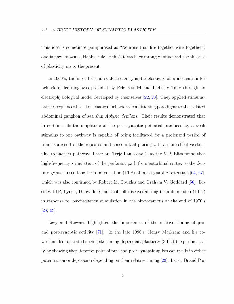
mentally. Figure 1.1 shows a comparison between experiments and the second type
of model.
5
1.2. MATHEMATICAL MODELS OF PLASTICITY
Figure 1.1: The STDP curve generated by the second type of Calcium-based modelwhich can determine the synaptic weights evolution efficiency. From Rubin et al.,2005[57]. Experimental data points from Bi and Poo,1998 [27].
Donald Hebb postulated in 1949 that a synaptic connection between two neurons
is potentiated when a pre-synaptic neuron is repeatedly implicated in the firing of
a post-synaptic cell, or, more generally, when a pre- and post-synaptic neuron are
active simultaneously. Terrence Sejnowski suggested spike-time correlations as a
requirement for synaptic plasticity in 1977 [66]. In 1993, Wulfram Gerstner and
colleagues proved that, for a recurrent network to learn spatio-temporal patterns,
instead of firing rates, plasticity needs to be based on spike times [70], and, a few years
later, proposed spike-timing plasticity models for sound localization [69]. The STDP
learning rule have been shown to feed forward artificial neural networks capable of
pattern recognition, and have been used to recognize traffic, sound or movement
using Dynamic Vision Sensor cameras [9, 65, 49]. Such learning rules can be mapped
to equivalent rate-based rules under the assumption of stationary Poisson statistics
for the firing times of pre- and postsynaptic neurons [52]. We can also relate STDP to
a nonlinear rate model where the weight change depends linearly on the presynaptic
rate, but nonlinearly on the postsynaptic rate [21]. There are two ways to achieve
6
1.2. MATHEMATICAL MODELS OF PLASTICITY
this. One way is to is to implement standard STDP with nearest-neighbor instead of
all-to all coupling. This gives a nonlinearity consistent with the BCM rule [32]. The
other way is using a triplet STDP rule instead of the standard pair-based rule. The
triplet STDP rule can become identical to the BCM rule under certain cases [21].
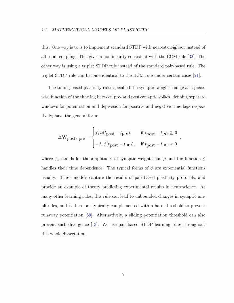
The timing-based plasticity rules specified the synaptic weight change as a piece-
wise function of the time lag between pre- and post-synaptic spikes, defining separate
windows for potentiation and depression for positive and negative time lags respec-
tively, have the general form:
∆Wpost←pre =
f+φ(tpost − tpre), if tpost − tpre ≥ 0
−f−φ(tpost − tpre), if tpost − tpre < 0
,
where f± stands for the amplitudes of synaptic weight change and the function φ
handles their time dependence. The typical forms of φ are exponential functions
usually. These models capture the results of pair-based plasticity protocols, and
provide an example of theory predicting experimental results in neuroscience. As
many other learning rules, this rule can lead to unbounded changes in synaptic am-
plitudes, and is therefore typically complemented with a hard threshold to prevent
runaway potentiation [59]. Alternatively, a sliding potentiation threshold can also
prevent such divergence [13]. We use pair-based STDP learning rules throughout
this whole dissertation.
7

1.3. MOTIVATION OF THIS DISSERTATION
1.3 Motivation of this dissertation
Many studies have explored how STDP shapes the distribution of synaptic weights
of a group of synaptic connection to a a single neuron [58, 47, 53, 51, 3]. Here, we
consider the more challenging problem of understanding how STDP shapes the glob-
al structure of a recurrent network of spiking neurons. Related questions have been
addressed before in a number of studies [59, 17, 1, 18, 39, 40, 41, 42, 43, 44, 33, 11].
The generally antisymmetric shape of the STDP window, in which reversing the or-
dering of pre- and postsynaptic spikes reverses the direction of synaptic change, led
to the proposal that this synaptic modification rule should eliminate strong recur-
rent connections between neurons [59, 37]. This idea has been expanded by Kozloski
and Cecchi [33] to larger polysynaptic loops in the case of balanced STDP which
the magnitudes of potentiation and depression are equal. The case of enhancing
recurrent connections through pair-based STDP was also proposed by Song and Ab-
bott [59] and was explored by Clopath and colleagues [11] later in a more complex
model. Clopath and her colleagues proposed a STDP model in which the synaptic
changes depend on presynaptic spike arrival and the postsynaptic membrane poten-
tial, filtered with two different time constants. They use this model to explain the
connectivity patterns in cortex with a few strong bidirectional connections. Their
plasticity rule lead not only to development of localized receptive fields but also to
connectivity patterns that reflect the neural code. An excessively active group of
neurons has been shown to decouple from the rest of the network through STDP [1],
and in presence of axonal delays, STDP enhances recurrent connections when the
neurons fire in a tonic irregular mode [18].
8
1.3. MOTIVATION OF THIS DISSERTATION
Babadi and Abbott have shown that large network properties can be explained by
the effect of STDP on pairwise interactions of Poisson neurons based on the baseline
firing rates [4]. They begin with analyzing the vector fields of the synaptic weights
for two-cell recurrent symmetric (2 cells with the same baseline firing rate), and
asymmetric (with different rates) networks under the influence of balanced and un-
balanced (potentiation dominated and depression dominated) Hebbian STDP rules.
Based on this analysis, they were able to make predictions about the dynamics of
weights in large networks, and found that potentiation dominated STDP rules will
generate loops while depression dominated rules will eliminate loops. Moreover, they
showed that rightward shifted STDP can generate recurrent connections, and STDP
with leftward shift generates loops at higher firing rates but eliminates loops at low-
er rates. This work provided a clear picture of how local learning rules can shape
network dynamics from simple neuron circuits.
Gilson and his colleagues used a theoretical framework based on the assumption
that spike trains can be described as Poisson processes, and used this framework
to analytically describe the network dynamics and the evolution of the synaptic
weights in a series of five papers [39, 40, 41, 42, 43]. They apply STDP to some of the
synaptic connections in a network driven by two pools of input spike trains that have
homogeneous within-pool firing rates and spike-time correlations. In the first paper,
they found that the weights from the more correlated inputs are potentiated. In the
second paper, they showed that the presence of fixed excitatory recurrent connections
between neurons makes neurons tend to select the same input pool. They showed
that, in the absence of external inputs, STDP can nevertheless generate structure
9

1.3. MOTIVATION OF THIS DISSERTATION
in the network through autocorrelation effects in the third paper. In the fourth
paper, they illustrated that, for a network receiving fixed input weights which are
stimulated by external spike trains, STDP can lead to both a stabilization of all the
neuron firing rates and a robust weight specialization. In the last paper, they showed
that a recurrently connected network stimulated by external pools can divide into
two groups of neurons under the effect of STDP.
Most of these previous studies were based on the Poisson neuron model. However,
while the assumption of a Poisson neuron leads to tractable models, it also does not
fully reflect a number of properties of actual neurons. One of the main issues is
the noise in neuronal firing. While a Poisson model captures such noise indirectly
through the probabilistic nature of the firing of spikes, it does not capture explicitly
the internally generated and synaptic noise. Thus it does not provide a mechanistic
explanation of neuronal response variability. Spike generation, by itself, is highly
reliable and deterministic. However, noise in neural responses is believed to result
in part from the fact that synapses are very unreliable [10]. Noise is therefore due
to unreliable synapses, or inherited from the input from the rest of the network, and
is not due to spike generation. In the integrate-and-fire neuron model, the output is
a filtered, thresholded and deterministic function of the input. Thus, the integrate-
and-fire model captures many of the qualitative features, and is often used as a
starting point for conceptualizing the biophysical behavior of single neurons [62].
There is evidence showing that some cells respond as integrate-and-fire neurons
[55]. This implies such model is more close to the real neurons. Here we consider
networks built of this general type of neurons - EIF (exponential integrate-and-fire)
10

1.3. MOTIVATION OF THIS DISSERTATION
neurons [25], which have been shown to match spiking dynamics well in certain
cortical areas [7]. We find some new properties for the networks even if the baseline
firing rates of the neurons are all the same, which can not be captured by networks
of Poisson neurons.
11

CHAPTER 2
Methods
We consider networks of EIF neurons with the same baseline firing rate but where
each cell receives different levels of background noise, which is driven by noise with
mean µ and standard deviation σ. The properties of background noise are common
to many neurons, so they provide a natural starting point. For fixed baseline firing
rate, based on the values of µ and σ, there are two main regimes for EIF neurons:
noise driven (higher σ value and lower µ value) and stimulus driven (lower σ value
and higher µ value). The spikes of EIF neurons are mainly driven by the noise (σ) in
the former regime while the stimulus (µ) is dominant in the latter regime. A neuron
is said to be excitable when the direct input, µ results in membrane voltage that is
12
2.1. THE EIF MODEL
close to threshold. In this case small fluctuations in membrane voltage, whether due
to input or noise internal to the cell, can cause the neuron to fire.
Our goal is to study the impact of STDP rules on the evolution of weights in a
network. To do so, we start with networks of two cells. We use linear response theo-
ry to determine the cross-covariance function between the cells in the network. It is
essential that we require the weights change slowly compared to network dynamics,
which provides a separation of time scales (2.3). In turn, this allows us to determine
how the weights evolve. Moreover, this also allows us to generalize the approach
described in [34] to networks in which the weights are changing by analyzing their
cross-covariance functions or phase planes (vector fields), and use these to predict
the behavior of large networks. We test our predictions in large networks using both
our theoretical framework, and direct numerical simulations.
2.1 The EIF model
All of the the networks we considered are composed of EIF (exponential integrate-
and-fire) neurons. The membrane potentials Vi is thus modeled by
CmdVidt
= gL(VL − Vi) + gLψ(Vi) + Ii(t) + fi(t) . (2.1)
13
2.1. THE EIF MODEL
Here Cm is the membrane capacitance, VL is the leak reversal potential, and gL is
the membrane conductance.
ψ(Vi) = ∆T exp
[Vi − VT
∆T
]
is the exponential term. Here VT is the soft threshold. ∆T shapes the spiking
dynamics of the membrane potential. Ii(t) = µi + gLσiD(√
(1− c)ξi(t) +√cξc(t)) is
the input term. D =√
2CmgL
, ξi(t) models background white noise with mean µi and
standard deviation σi, ξc(t) is the external common white noise input, and c ∈ [0, 1]
is the scaling parameter. When c = 0 the neurons in the network receive independent
background white noise input. When c = 1 this background noise is identical in all
cells. Here we choose to use the EIF neuron model because it accurately predicts the
statistical features of spike trains for a large class of pyramidal neurons [35].
A post–synaptic input current is generated whenever a presynaptic cell spikes.
We assume the synaptic kernels are exponential, and thus have the form:
Jij(t) = WijH(t− τD)exp
[− t− τD
τS
].
Here H is the heaviside step function, τD is the synaptic delay, τS is the synaptic
time constant. The matrix W defines the synaptic weights, and the entry Wij de-
notes the weight of the directed connection from neuron j to neuron i. Therefore,
yj(t) = Σkδ(t − tj,k) is the output spike train of cell j, then the synaptic current in
cell i generated by the spiking of cell j is given by fi(t) = Σj(Jij ∗ yj)(t).
14

2.1. THE EIF MODEL
A Poisson neuron is completely described by its firing rate [60]. However, the
dynamics and response of the EIF neuron are governed by parameters that capture
the physiological properties of the cell. Here we will concentrate on two parameters,
the mean µ and standard deviation σ of the input. These two parameters both affect
the firing rate, and the variability of the neuron’s output [38]. The same firing rate
can be achieved for different µ and σ values (Figure 2.1). The variability in the
output is not the same however. The statistics of the spike trains can be different
according to the µ and σ values (Figure 2.2). Moreover, CV (coefficient of variation,
the ratio of the standard deviation σ to the mean µ, σµ) can vary even if the firing rate
stays the same. As we will see below, this makes STDP in such networks more subtle.
(a)
06
50
rate
s (H
z)
4 200
7 (mV)
100
150
<2 (mV 2 )
2 10050
(b)
7.52
15 22.5
30.1 37.6
45.1 52.6
60.167.6
75.282.7
90.297.7
105113
50 100 150 200
<2 (mV 2)
1
2
3
4
5
6
7 (
mV
)
Figure 2.1: Different µ-σ values can attain the same baseline firing rate.(A) Changes of baseline firing rate according to µ and σ values. (B) Bottom of (A),illustrating that different µ and σ values can attain the same baseline firing rate.
15

2.1. THE EIF MODEL
(a) (b) (c)
Figure 2.2: Neurons with the same baseline firing rate can have differentfiring statistics. (A) Different µ and σ values can attain the same baseline firingrate 7.6 Hz. (B) EIF neurons with the same baseline firing rate 7.6 Hz and higher µwill generate more regular spike train. (C) Neurons with lower µ will generate lessregular spike train.
In Table 2.1, we choose 5 different µ-σ pairs that lead to the same baseline firing
rate 7.6(Hz) as an example. Besides µ and σ, other parameters can also affect the
rates, such as the spiking dynamics shaping parameter ∆T in the exponential term
ψ(Vi). Higher ∆T causes more rapid spike onset, and leads to higher firing rates.
However, the impact of these other parameters is expected to be small compared to
µ and σ, the parameters that are the focus of our study.
Pair index µ (mV) σ2 (mV2) Fano factor Baseline firing rate (Hz)1 1.37 49 0.772 1.19 64 0.813 1 81 0.84 7.64 0.81 100 0.885 0.61 121 0.91
Table 2.1: 5 different µ-σ pairs that attain the same baseline firing rate 7.6(Hz). Redrow is our baseline setting for the neuron model.
16
2.2. THE HEBBIAN STDP RULE
We take the red pair as our baseline setting. Table 2.1 thus shows that to obtain
the same baseline firing rate when we increase σ, we need to lower µ.
2.2 The Hebbian STDP rule
To study how plasticity shapes the structure of the network, we use a well-known
model of STDP [69], which has been supported by experimental evidence starting
with that of Bi and Poo in 1998 [27], and followed by other studies [72, 2, 68]. If we
denote by s the time difference between the pre- and post-synaptic spikes
s = tpost − tpre = tj − ti ,
then we can define a Hebbian STDP rule by
∆Wji(s) =
W0
jiH(Wmax −Wji)L(s) , if s ≥ 0
W0jiH(Wji)L(s) , if s < 0
, (2.2)
where
L(s) =
f+e
− |s|τ+ , if s ≥ 0
−f−e− |s|τ− , if s < 0
.
Here H(x) is the Heaviside function, f+ > 0 and f− > 0 are the amplitudes of
17

2.3. WEIGHT CHANGE DYNAMICS
potentiation and depression respectively, τ+ and τ− are the time constants, Wmax is
the upper bound of the synaptic weights and W0 is the binary adjacency matrix of
the network, enforcing that STDP rule can only modify connections that exist in the
network structure.
We also consider an Anti-Hebbian STDP rule, which is similar to the Hebbian
STDP rule and the only difference is the potentiation and depression sides are re-
versed. We use these rules in a number of examples we describe below, although our
approach is applicable to any other pairwise STDP rules.
2.3 Weight change dynamics
We can denote the spiking output of a neuron i by
yi(t) =
ni∑i=1
δ(t− ti) . (2.3)
According to [52, 37, 44, 3], we can build the bridge from the joint statistics of yi(t)
and yj(t) to the evolution of synaptic weights. The learning rule given in Eq.(2.2)
governs the changes of the synaptic weight Wji (from neuron i to neuron j). Let
∆TWji be the total change in the related synaptic weight during a time interval of
length T . This weight change is calculated by summing the contributions of input
18
2.3. WEIGHT CHANGE DYNAMICS
(i) and output (j) spikes occurring in the time interval [t, t+ T ]. We have
∆TWji =
ˆ t+T
t
ˆ t+T
t
∆Wji(t2 − t1)yj(t2)yi(t1)dt2dt1 .
Let s = t2−t1, 〈·〉 denote the trial average, then the trial-averaged rate of synaptic
weight change is
〈∆TWji〉T
=1
T
ˆ t+T
t
ˆ t+T−t1
t−t1∆Wji(s)〈yj(t1 + s)yi(t1)〉dsdt1 . (2.4)
The trial-averaged spike train cross-covariance Cji(s) is
Cji(s) =1
T
ˆ t+T
t
〈yj(t1 + s)yi(t1)〉dt1 − rirj ,
where rj and ri are the stationary firing rates for neuron j and i respectively. Using
this term in Eq.(2.4), we get
〈∆TWji〉T
=
ˆ t+T−t1
t−t1∆Wji(s)(Cji(s) + rjri)ds . (2.5)
We define the widthW of the learning rule ∆Wji(s) and let T �W . Then most
of the contributions to the weights evolution of the learning rule should be inside
the interval [−W ,W ]. Thus, we can extend the integration over s in Eq.(2.5) to run
from −∞ to +∞. We require the amplitude of individual changes in the synaptic
weights to be small (f± � Wmax). So the value of Wji do not change much in the
time interval of length T . Thus T separates the time scale W from the time scale of
19
2.3. WEIGHT CHANGE DYNAMICS
the learning dynamics, which allows us to approximate the left-hand side of Eq.(2.5)
by the rate of changedWji
dt:
dWji
dt=
ˆ +∞
−∞∆Wji(s)(Cji(s) + rjri)ds
=
ˆ +∞
−∞∆Wji(s)Cji(s)ds︸ ︷︷ ︸
1
+ rjri
ˆ +∞
−∞∆Wji(s)ds︸ ︷︷ ︸2
. (2.6)
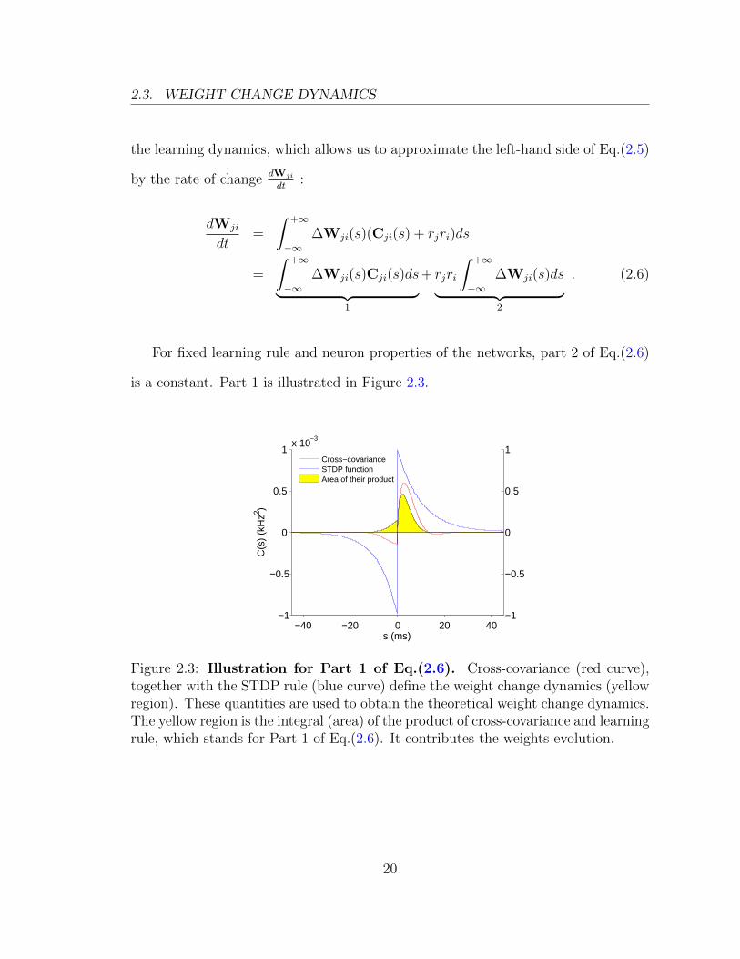
For fixed learning rule and neuron properties of the networks, part 2 of Eq.(2.6)
is a constant. Part 1 is illustrated in Figure 2.3.
−40 −20 0 20 40−1
−0.5
0
0.5
1x 10
−3
C(s
) (k
Hz2 )
s (ms)
Cross−covarianceSTDP functionArea of their product
−1
−0.5
0
0.5
1
Figure 2.3: Illustration for Part 1 of Eq.(2.6). Cross-covariance (red curve),together with the STDP rule (blue curve) define the weight change dynamics (yellowregion). These quantities are used to obtain the theoretical weight change dynamics.The yellow region is the integral (area) of the product of cross-covariance and learningrule, which stands for Part 1 of Eq.(2.6). It contributes the weights evolution.
20

2.4. APPROXIMATING CROSS-COVARIANCES USING LINEAR RESPONSETHEORY
2.4 Approximating cross-covariances using linear
response theory
We will briefly introduce an approximation method to estimate the pairwise spike
train cross-covariances Cij(s) using a synaptic weight matrix W [5, 6, 34, 48]. We
consider the Fourier transform of a spike train (Eq.(2.3)),
yi(ω) =
ˆ ∞−∞
yi(t)e−2πiωtdt ,
where ω is frequency. Assuming the synaptic weights, Wij are weak, we can approx-
imate the spike response from neuron i (Eq.(2.1)) as:
yi(ω) ≈ y0i (ω) + Ai(ω)
( N∑j=1
Jij(ω)yj(ω)
). (2.7)
Here Ai(ω) is Fourier transform of the linear response [12] of the post-synaptic neu-
ron i, measuring how strongly modulations in synaptic currents at frequency ω are
transferred into modulations of instantaneous firing rate about a background state
y0i (ω). The function Jij(ω) is the Fourier transform of a synaptic filter. Eq.(2.7) is
a linear approximation for how a neuron integrates and transforms a realization of
synaptic input into a spike train.
Following [5, 6, 34], we use this linear approximation to estimate the Fourier
transform of Cij(s), written as Cij(ω) =< yi(ω)y∗j(ω) >. Here y∗ denotes the
21
2.4. APPROXIMATING CROSS-COVARIANCES USING LINEAR RESPONSETHEORY
conjugate transpose. This yields the following matrix equation:
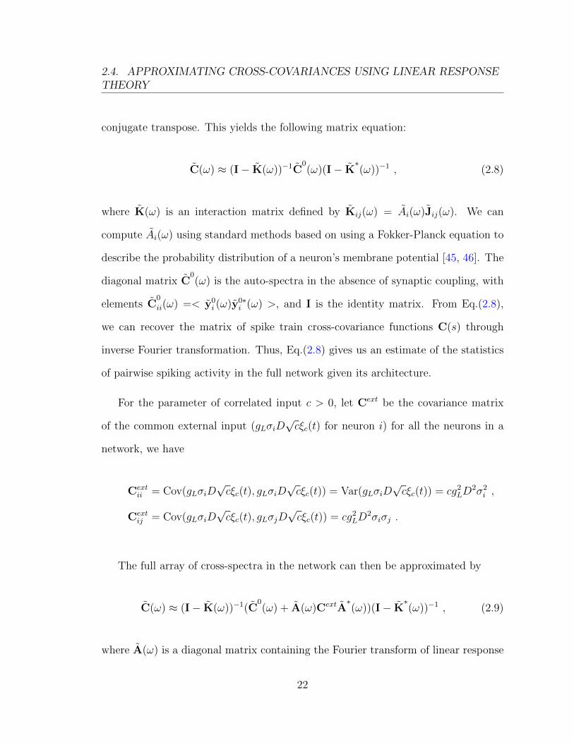
C(ω) ≈ (I− K(ω))−1C0(ω)(I− K
∗(ω))−1 , (2.8)
where K(ω) is an interaction matrix defined by Kij(ω) = Ai(ω)Jij(ω). We can
compute Ai(ω) using standard methods based on using a Fokker-Planck equation to
describe the probability distribution of a neuron’s membrane potential [45, 46]. The
diagonal matrix C0(ω) is the auto-spectra in the absence of synaptic coupling, with
elements C0
ii(ω) =< y0i (ω)y0∗
i (ω) >, and I is the identity matrix. From Eq.(2.8),
we can recover the matrix of spike train cross-covariance functions C(s) through
inverse Fourier transformation. Thus, Eq.(2.8) gives us an estimate of the statistics
of pairwise spiking activity in the full network given its architecture.
For the parameter of correlated input c > 0, let Cext be the covariance matrix
of the common external input (gLσiD√cξc(t) for neuron i) for all the neurons in a
network, we have
Cextii = Cov(gLσiD
√cξc(t), gLσiD
√cξc(t)) = Var(gLσiD
√cξc(t)) = cg2LD
2σ2i ,
Cextij = Cov(gLσiD
√cξc(t), gLσjD
√cξc(t)) = cg2LD
2σiσj .
The full array of cross-spectra in the network can then be approximated by
C(ω) ≈ (I− K(ω))−1(C0(ω) + A(ω)CextA
∗(ω))(I− K
∗(ω))−1 , (2.9)
where A(ω) is a diagonal matrix containing the Fourier transform of linear response
22

2.4. APPROXIMATING CROSS-COVARIANCES USING LINEAR RESPONSETHEORY
functions of each neuron (Ai(ω)s).
Examples comparing theoretical and simulated cross-covariances of simple cir-
cuits with two neurons are in Sections 3.1.1 and 3.1.2.
23

CHAPTER 3
Results for simple circuits
In this chapter we first study the evolution of synaptic weights in a system of two mu-
tually coupled neurons. We apply the theoretical approach described in the previous
section, and confirm the results numerically. Insights gained from the simple system
of two neurons allow us to understand how features of the linear response function
together with the shape of the STDP function together determine the evolution of
synaptic weights.
24
3.1. CROSS-COVARIANCES AND LEARNING FOR TWO-CELL NETWORKS
3.1 Cross-covariances and learning for two-cell net-
works
We first study the cross-covariances and evolution of synaptic weights in particular
two-cell networks. We then generalize the approach to larger networks in the follow-
ing chapter.
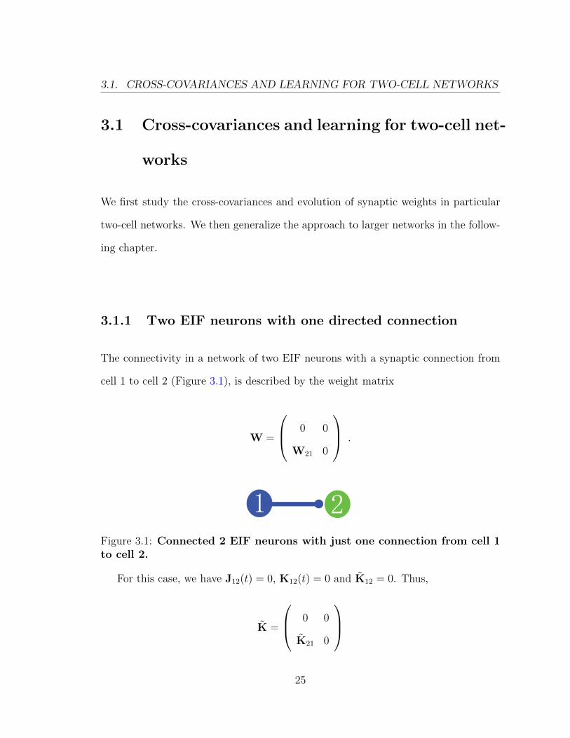
3.1.1 Two EIF neurons with one directed connection
The connectivity in a network of two EIF neurons with a synaptic connection from
cell 1 to cell 2 (Figure 3.1), is described by the weight matrix
W =
0 0
W21 0
.
1 2Figure 3.1: Connected 2 EIF neurons with just one connection from cell 1to cell 2.
For this case, we have J12(t) = 0, K12(t) = 0 and K12 = 0. Thus,
K =
0 0
K21 0
25
3.1. CROSS-COVARIANCES AND LEARNING FOR TWO-CELL NETWORKS
with K21 = A2J21. We therefore have, (I−K)−1 = (I+K), and similarly, (I−K∗)−1 =
(I + K∗).
The cross-spectrum matrix of the two processes is therefore given by Eq.(2.8),
C11 C12
C21 C22
≈ (I + K)
C0
11 0
0 C0
22
(I + K∗)
=
1 0
K21 1
C
0
11 0
0 C0
22
1 K
∗21
0 1
=
C0
11 K∗21C
0
11
K21C0
11 |K21|2C0
11 + C0
22
.
Thus, C21 ≈ K21C0
11 = A2J21C0
11, and C12 ≈ (A2J21)∗C
0
11. We can therefore use
inverse Fourier transforms to recover the cross-covariances, C12(t) ≈ F−1(C12)(t)
and C21(t) ≈ F−1(C21)(t).
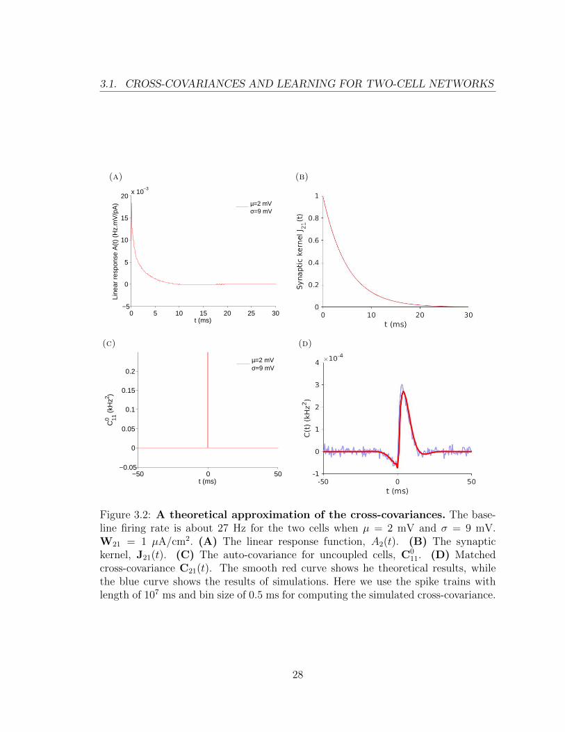
These equations show that the cross-covariances are determined by the linear
response function, Ai(t), the synaptic kernel Jij(t), as well as the uncoupled auto-
covariance C011. This is shown in Figure 3.2. This dependence can be presented
schematically as:
Linear response + Synaptic kernel + Uncoupled auto-covariance
→ Cross-covariances . (3.1)
26

3.1. CROSS-COVARIANCES AND LEARNING FOR TWO-CELL NETWORKS
In Figure 3.2, we show the linear response function, A2(t), the synaptic kernel,
J21(t), the uncoupled auto-covariance, C011, and the matched cross-covariance, C21(t).
As we have shown, the first three functions (panels A–C) can be combined to obtain
an approximation of the fourth (panel D). In Figure 3.2D, the red curve represents
this theoretical result obtained using Eq.(2.8), while the blue curve is obtained using
direct simulations of the stochastic differential equation Eq.(2.1). We use the same
color assignments to distinguish theoretical and simulation results below.
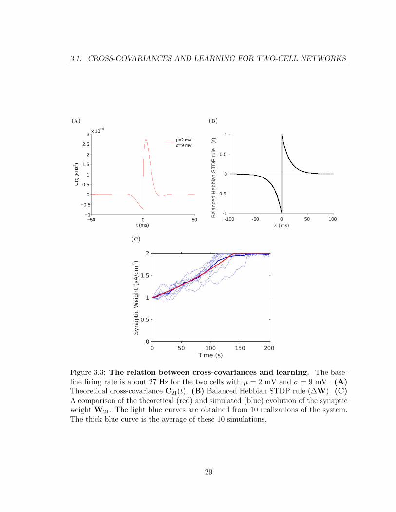
The dynamics of synaptic weights given by Eq.(2.6) is determined by the cross-
covariances, and the learning rule. This is illustrated in Figure 3.3. Note that a
change in synaptic weights affects the firing rate. In turn, this can affect the cross-
correlation, and the further evolution of the weights. We therefore need to recompute
the rates and linear responses for each update of synaptic weights. Thus this is a
closed loop - unlike in the Poisson neuron case.
In sum, we can complement the heuristic rule expressed in Eq.(3.1) by
Cross-covariance + Learning rule → Synaptic weight changes .
Figure 3.3A shows the theoretical cross-covariance, C21(t). Figure 3.3B shows
the balanced Hebbian STDP rule (f+ = f− and τ+ = τ− in Eq.(2.2)). The peak of
the cross-covariance is in the positive time domain. This is the potentiation side of
the balanced Hebbian STDP rule (See Figure 2.3). Due to the shape of the cross-
covariance and the learning rule, the synaptic weight W21 will be potentiated (Figure
3.3C).
27
3.1. CROSS-COVARIANCES AND LEARNING FOR TWO-CELL NETWORKS
(a)
0 5 10 15 20 25 30−5
0
5
10
15
20x 10
−3
t (ms)
Line
ar r
espo
nse
A(t
) (H
z.m
V/p
A)
µ=2 mVσ=9 mV
(b)
(c)
−50 0 50−0.05
0
0.05
0.1
0.15
0.2
t (ms)
C110
(kH
z2 )
µ=2 mVσ=9 mV
(d)
Figure 3.2: A theoretical approximation of the cross-covariances. The base-line firing rate is about 27 Hz for the two cells when µ = 2 mV and σ = 9 mV.W21 = 1 µA/cm2. (A) The linear response function, A2(t). (B) The synaptickernel, J21(t). (C) The auto-covariance for uncoupled cells, C0
11. (D) Matchedcross-covariance C21(t). The smooth red curve shows he theoretical results, whilethe blue curve shows the results of simulations. Here we use the spike trains withlength of 107 ms and bin size of 0.5 ms for computing the simulated cross-covariance.
28
3.1. CROSS-COVARIANCES AND LEARNING FOR TWO-CELL NETWORKS
(a)
−50 0 50−1
−0.5
0
0.5
1
1.5
2
2.5
3x 10
−4
t (ms)
C(t
) (k
Hz2 )
µ=2 mVσ=9 mV
(b)
-100 -50 0 50 100s (ms)
-1
-0.5
0
0.5
1
Bal
ance
d H
ebbi
an S
TD
P r
ule
L(s)
(c)
Figure 3.3: The relation between cross-covariances and learning. The base-line firing rate is about 27 Hz for the two cells with µ = 2 mV and σ = 9 mV. (A)Theoretical cross-covariance C21(t). (B) Balanced Hebbian STDP rule (∆W). (C)A comparison of the theoretical (red) and simulated (blue) evolution of the synapticweight W21. The light blue curves are obtained from 10 realizations of the system.The thick blue curve is the average of these 10 simulations.
29

3.1. CROSS-COVARIANCES AND LEARNING FOR TWO-CELL NETWORKS
3.1.2 Two EIF neurons with recurrent connections
For the network formed by two EIF neurons with recurrent connections shown in
Figure 3.4, we have the synaptic weight matrix
W =
0 W12
W21 0
.
1 2
Figure 3.4: Two EIF neurons with recurrent connections.
In this case,
K =
0 K12
K21 0
with K21 = A2J21 and K12 = A1J12.
Similarly,
(I− K)−1 =1
1− K12K21
(I + K) , and (I− K∗)−1 =
1
1− K∗12K
∗21
(I + K∗) ,
30
3.1. CROSS-COVARIANCES AND LEARNING FOR TWO-CELL NETWORKS
and so,
C11 C12
C21 C22
≈ 1
(1− K12K21)(1− K∗12K
∗21)
(I + K)
C0
11 0
0 C0
22
(I + K∗)
=1
|1− K12K21|2
1 K12
K21 1
C
0
11 0
0 C0
22
1 K
∗21
K∗12 1
=
1
|1− K12K21|2
C0
11 + |K12|2C0
22 K∗21C
0
11 + K12C0
22
K21C0
11 + K∗12C
0
22 |K21|2C0
11 + C0
22
.
This implies
C12 ≈K∗21C
0
11 + K12C0
22
|1− K12K21|2=
(A2J21)∗C
0
11 + A1J12C0
22
|1− A1J12A2J21|2
and
C21 ≈K21C
0
11 + K∗12C
0
22
|1− K12K21|2=A2J21C
0
11 + (A1J12)∗C
0
22
|1− A1J12A2J21|2.
We can rewrite these expressions as geometric series,
1
1− K12K21
=∞∑k=0
(K12K21)k ,
1
1− K∗12K
∗21
=∞∑l=0
(K∗12K
∗21)
l ,
31
3.1. CROSS-COVARIANCES AND LEARNING FOR TWO-CELL NETWORKS
to obtain
1
|1− K12K21|2=
1
(1− K12K21)(1− K∗12K
∗21)
=
( ∞∑k=0
(K12K21)k
)( ∞∑l=0
(K∗12K
∗21)
l
)=
∞∑k,l=0
(K12K21)k(K
∗12K
∗21)
l .
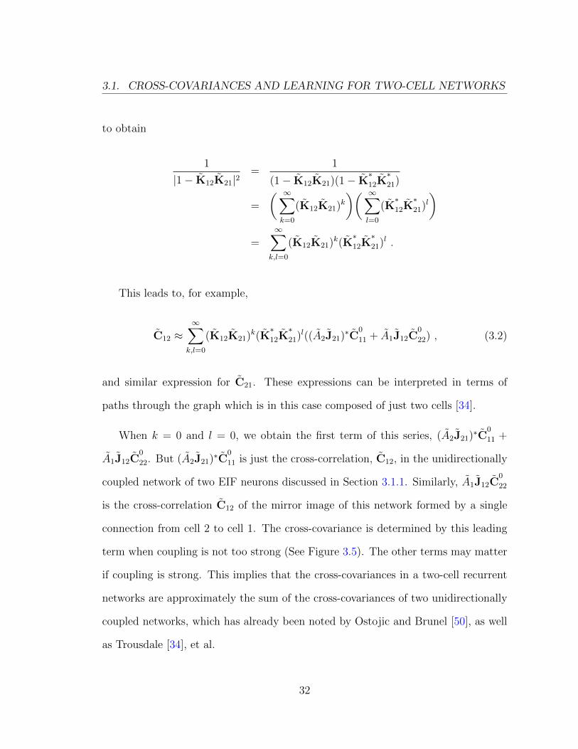
This leads to, for example,
C12 ≈∞∑
k,l=0
(K12K21)k(K
∗12K
∗21)
l((A2J21)∗C
0
11 + A1J12C0
22) , (3.2)
and similar expression for C21. These expressions can be interpreted in terms of
paths through the graph which is in this case composed of just two cells [34].
When k = 0 and l = 0, we obtain the first term of this series, (A2J21)∗C
0
11 +
A1J12C0
22. But (A2J21)∗C
0
11 is just the cross-correlation, C12, in the unidirectionally
coupled network of two EIF neurons discussed in Section 3.1.1. Similarly, A1J12C0
22
is the cross-correlation C12 of the mirror image of this network formed by a single
connection from cell 2 to cell 1. The cross-covariance is determined by this leading
term when coupling is not too strong (See Figure 3.5). The other terms may matter
if coupling is strong. This implies that the cross-covariances in a two-cell recurrent
networks are approximately the sum of the cross-covariances of two unidirectionally
coupled networks, which has already been noted by Ostojic and Brunel [50], as well
as Trousdale [34], et al.
32
3.1. CROSS-COVARIANCES AND LEARNING FOR TWO-CELL NETWORKS
(a)
1 2
(b)
1 2(c)
1 2
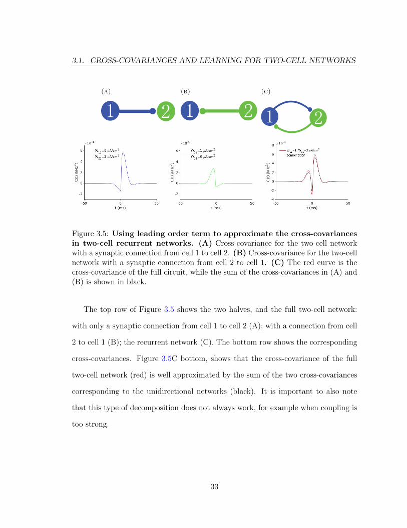
Figure 3.5: Using leading order term to approximate the cross-covariancesin two-cell recurrent networks. (A) Cross-covariance for the two-cell networkwith a synaptic connection from cell 1 to cell 2. (B) Cross-covariance for the two-cellnetwork with a synaptic connection from cell 2 to cell 1. (C) The red curve is thecross-covariance of the full circuit, while the sum of the cross-covariances in (A) and(B) is shown in black.
The top row of Figure 3.5 shows the two halves, and the full two-cell network:
with only a synaptic connection from cell 1 to cell 2 (A); with a connection from cell
2 to cell 1 (B); the recurrent network (C). The bottom row shows the corresponding
cross-covariances. Figure 3.5C bottom, shows that the cross-covariance of the full
two-cell network (red) is well approximated by the sum of the two cross-covariances
corresponding to the unidirectional networks (black). It is important to also note
that this type of decomposition does not always work, for example when coupling is
too strong.
33
3.1. CROSS-COVARIANCES AND LEARNING FOR TWO-CELL NETWORKS
(a)
0 5 10 15 20 25 30−5
0
5
10
15
20x 10
−3
t (ms)
Line
ar r
espo
nse
Ai(t
) (H
z.m
V/p
A)
A1(t) for cell 1
A2(t) for cell 2
(b) (c)
−50 0 50−0.05
0
0.05
0.1
0.15
0.2
t (ms)
Cii0 (
kHz2 )
C011
(t)
C022
(t)
(d) (e)
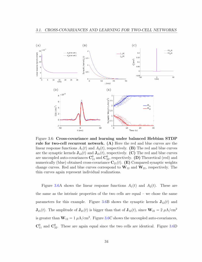
Figure 3.6: Cross-covariance and learning under balanced Hebbian STDPrule for two-cell recurrent network. (A) Here the red and blue curves are thelinear response functions A1(t) and A2(t), respectively. (B) The red and blue curvesare the synaptic kernels J12(t) and J21(t), respectively. (C) The red and blue curvesare uncoupled auto-covariances C0
11 and C022, respectively. (D) Theoretical (red) and
numerically (blue) obtained cross-covariance C21(t). (E) Compared synaptic weightschange curves. Red and blue curves correspond to W12 and W21, respectively. Thethin curves again represent individual realizations.
Figure 3.6A shows the linear response functions A1(t) and A2(t). These are
the same as the intrinsic properties of the two cells are equal – we chose the same
parameters for this example. Figure 3.6B shows the synaptic kernels J12(t) and
J21(t). The amplitude of J21(t) is bigger than that of J12(t), since W21 = 2 µA/cm2
is greater than W12 = 1 µA/cm2. Figure 3.6C shows the uncoupled auto-covariances,
C011 and C0
22. These are again equal since the two cells are identical. Figure 3.6D
34
3.1. CROSS-COVARIANCES AND LEARNING FOR TWO-CELL NETWORKS
compares the cross-covariance C21(t) obtained from simulations (blue) and theory
(red). The peak with the higher amplitude is in the positive time domain, which is
on the potentiation side of our Hebbian STDP rule (Figure 3.3B). With a symmetric
learning rule this implies that potentiation of W21 is dominant, which will lead to
an increase in W21, while W12 will decrease in time. Figure 3.6E shows W12 and
W21 obtained using theory and simulations with a symmetric Hebbian STDP rule.
The asymmetry of the cross-covariances seen in Figure 3.5 and 3.6 is due to
the different initial weights of the two synaptic connections. Asymmetric cross-
covariances can also occur when the connection weights and firing rates are equal,
but the intrinsic properties, as determined by the parameters µ and σ, differ between
the cells. This is illustrated in Figure 3.7.
Here we fixed the baseline firing rate of both cells at 27 Hz. This occurs both
when µ = 2 mV and σ = 9 mV, and when µ = 2.37 mV and σ = 5 mV (note that
firing rates can be equal for different µ and σ values, as shown in Figure 2.1 and
Table 2.1). We also set both synaptic weights to 2 µA/cm2. We consider two cases:
two cells with the same and two cells with different setting of the parameters µ and
σ. When we use µ = 2 mV and σ = 9 mV for both cells we have symmetric cross-
covariances (Figure 3.7B). With µ = 2 mV and σ = 9 mV for cell 1 and µ = 2.37 mV
and σ = 5 mV for cell 2 we see that the amplitude of the linear response function
for cell 2 (A2(t) (blue)) is larger than that for cell 1 (Figure 3.7D). This means that,
even when the baseline firing rates are equal, the cell with lower σ (or higher µ value)
will have a linear response function of bigger amplitude. That is, lower noise makes
a cell more sensitive to its inputs, and hence a larger peak in the linear response.
35

3.1. CROSS-COVARIANCES AND LEARNING FOR TWO-CELL NETWORKS
(a)
0 5 10 15 20 25 30−0.005
0
0.005
0.01
0.015
0.02
0.025
t (ms)
Line
ar r
espo
nse
Ai(t
) (H
z.m
V/p
A)
A1(t) for cell 1: σ = 9 mV
A2(t) for cell 2: σ = 9 mV
(b)
-50 0 50t (ms)
-6
-4
-2
0
2
4
6
8
C(t
) (k
Hz
2)
#10 -4
(c)
τ
f
10 11 12 13 14 15 16 17 18 19 20
0.01
0.02
0.03
0.04
0.05
0.06
0.07
0.08
0.09
0.10.2
0.4
0.6
0.8
1
1.2
1.4
1.6
1.8
x 10−4
(d)
0 5 10 15 20 25 30−0.005
0
0.005
0.01
0.015
0.02
0.025
0.03
t (ms)
Line
ar r
espo
nse
Ai(t
) (H
z.m
V/p
A)
A1(t) for cell 1: σ = 9 mV
A2(t) for cell 2: σ = 5 mV
(e)
-50 0 50t (ms)
-1
-0.5
0
0.5
1
1.5
C(t
) (k
Hz
2)
#10 -3
(f)
τ
f
10 11 12 13 14 15 16 17 18 19 20
0.01
0.02
0.03
0.04
0.05
0.06
0.07
0.08
0.09
0.10.2
0.4
0.6
0.8
1
1.2
1.4
1.6
1.8
x 10−4
Figure 3.7: Different intrinsic properties of neurons lead to asymmetriccross-covariances, and, in turn, affect the evolution of synaptic weights.(A,D) Linear response functions for the two cells with the same setting and differentsetting respectively. (B,E) cross-covariance C21(t) for the two cells with the samesetting and different setting respectively. (C,F) Integrals of the product of cross-covariances C21(t) and different learning rules for the two cells with the same settingand different setting respectively.
This difference in linear responses breaks the symmetry of the cross-covariances.
With equal synaptic weights, A2(t) governs the peak of C21(t) (spike times of cell
1 as reference) in the positive time domain while A1(t) controls the peak in the
negative time domain. The amplitude of A2(t) is bigger than that of A1(t) implying
the amplitude of the peak in the positive time domain will be bigger than that in the
negative time domain. This leads to the asymmetry of the cross-covariances which
is apparent in Figure 3.7E.
36

3.1. CROSS-COVARIANCES AND LEARNING FOR TWO-CELL NETWORKS
The shape of the cross-covariances affects the evolution of the synaptic weights. In
the right column of Figure 3.7, we show the integrals of the product of corresponding
cross-covariances and different learning rules. Here we used a balanced leaning rule
with f = f+ = f−, τ = τ+ = τ−, and varied f and τ . For symmetric cross-covariance,
the integral is always 0. However, for asymmetric cross-covariances, it changes with
f and τ . We can see that the integral increases with f and τ (Figure 3.7F). This
implies that the learning rule with bigger amplitude (f) and broader shape (τ) will
make the synaptic weight changes more sensitive to the cross-covariance.
In this case, under fixed baseline firing rate, the differences in the properties of
the individual cells result in an asymmetric cross-covariance, and thus impact the
evolution of their coupling weights according to the applied learning rule. Cross-
covariances and learning rules shape the network structure together, and both are
important here. However, the Poisson neuron model does not exhibit this behavior,
as the properties of this neuron are determined by the baseline firing rate only.
37

3.1. CROSS-COVARIANCES AND LEARNING FOR TWO-CELL NETWORKS
3.1.3 Two EIF neurons with recurrent connections and com-
mon input
In a recurrent two-cell network with common input to the two cells, Eq.(2.9), gives
the uncoupled auto-spectrum as:
C0
+ ACextA∗
=
C0
11 0
0 C0
22
+ cg2LD2
A1 0
0 A2
σ2
1 σ1σ2
σ2σ1 σ22
A∗1 0
0 A∗2
=
C0
11 + cg2LD2σ2
1|A1|2 cg2LD2σ1σ2A1A
∗2
cg2LD2σ1σ2A2A
∗1 C
0
22 + cg2LD2σ2
2|A2|2
.
Therefore,
C11 C12
C21 C22
≈ 1
|1− K12K21|2 1 K12
K21 1
C
0
11 + cg2LD2σ2
1|A1|2 cg2LD2σ1σ2A1A
∗2
cg2LD2σ1σ2A2A
∗1 C
0
22 + cg2LD2σ2
2|A2|2
1 K
∗21
K∗12 1
=
1
|1− K12K21|2
C0
11 + |K12|2C0
22 + cg2LD2P1 K
∗21C
0
11 + K12C0
22 + cg2LD2P2
K21C0
11 + K∗12C
0
22 + cg2LD2P3 |K21|2C
0
11 + C0
22 + cg2LD2P4
,
38
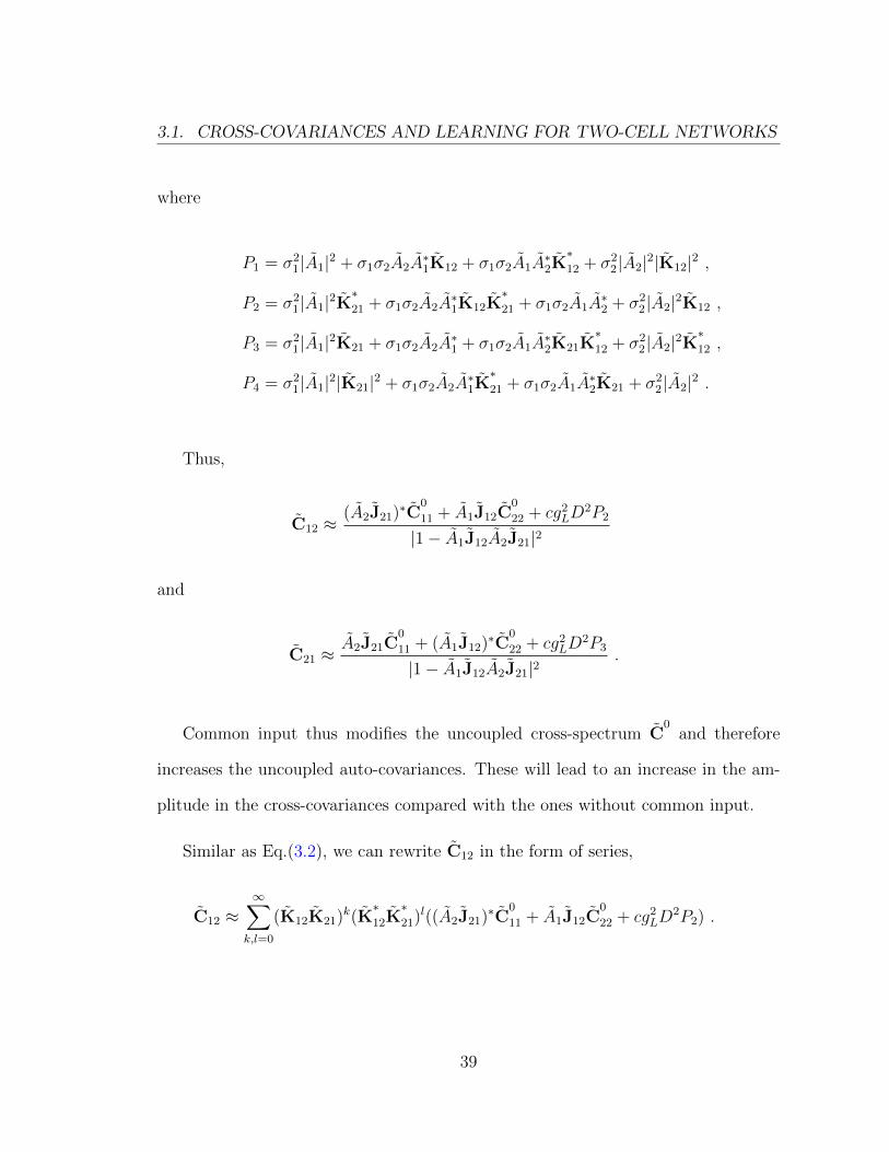
3.1. CROSS-COVARIANCES AND LEARNING FOR TWO-CELL NETWORKS
where
P1 = σ21|A1|2 + σ1σ2A2A
∗1K12 + σ1σ2A1A
∗2K∗12 + σ2
2|A2|2|K12|2 ,
P2 = σ21|A1|2K
∗21 + σ1σ2A2A
∗1K12K
∗21 + σ1σ2A1A
∗2 + σ2
2|A2|2K12 ,
P3 = σ21|A1|2K21 + σ1σ2A2A
∗1 + σ1σ2A1A
∗2K21K
∗12 + σ2
2|A2|2K∗12 ,
P4 = σ21|A1|2|K21|2 + σ1σ2A2A
∗1K∗21 + σ1σ2A1A
∗2K21 + σ2
2|A2|2 .
Thus,
C12 ≈(A2J21)
∗C0
11 + A1J12C0
22 + cg2LD2P2
|1− A1J12A2J21|2
and
C21 ≈A2J21C
0
11 + (A1J12)∗C
0
22 + cg2LD2P3
|1− A1J12A2J21|2.
Common input thus modifies the uncoupled cross-spectrum C0
and therefore
increases the uncoupled auto-covariances. These will lead to an increase in the am-
plitude in the cross-covariances compared with the ones without common input.
Similar as Eq.(3.2), we can rewrite C12 in the form of series,
C12 ≈∞∑
k,l=0
(K12K21)k(K
∗12K
∗21)
l((A2J21)∗C
0
11 + A1J12C0
22 + cg2LD2P2) .
39
3.1. CROSS-COVARIANCES AND LEARNING FOR TWO-CELL NETWORKS
The leading term in this series is (A2J21)∗C
0
11 + A1J12C0
22 + cg2LD2P2. In this
leading term, the summand (A2J21)∗C
0
11 is just the cross-covariance C12 of the net-
work formed by two EIF neurons with a synaptic connection from cell 1 to cell 2, but
without common input. A1J12C0
22 is C12 of the network for reversed case (connection
from cell 2 to cell 1 without common input). The last summand, cg2LD2P2, contains
the term cg2LD2σ1σ2A1A
∗2, which is the cross-covariance C12 between cell 1 and cell
2 with common input in the absence of synaptic connections between the cells.
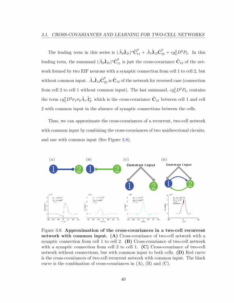
Thus, we can approximate the cross-covariances of a recurrent, two-cell network
with common input by combining the cross-covariances of two unidirectional circuits,
and one with common input (See Figure 3.8).
(a)
1 2
(b)
1 2
(c)
1 2
Common Input(d)
1 2
Common Input
Figure 3.8: Approximation of the cross-covariances in a two-cell recurrentnetwork with common input. (A) Cross-covariance of two-cell network with asynaptic connection from cell 1 to cell 2. (B) Cross-covariance of two-cell networkwith a synaptic connection from cell 2 to cell 1. (C) Cross-covariance of two-cellnetwork without connections, but with common input to both cells. (D) Red curveis the cross-covariances of two-cell recurrent network with common input. The blackcurve is the combination of cross-covariances in (A), (B) and (C).
40

3.1. CROSS-COVARIANCES AND LEARNING FOR TWO-CELL NETWORKS
Figure 3.8 is similar to the Figure 3.5 in the previous section. The figure illus-
trates that in a two-cell recurrent network with common input, we can also use the
cross-covariances of simpler, uni-directional circuits, along with the cross-covariance
generated by the common input to approximate the full cross-covariance.
(a) (b)
(c) (d) (e)
Figure 3.9: Cross-covariances and synaptic weight dynamics under bal-anced Hebbian STDP in a two-cell, recurrently coupled network withcommon input. (A) Cross-covariances between the cells with (red) and without(blue) common input. (B) Comparison of cross-covariance with common input (redcurve in (A)) obtained analytically and numerically. (C) Theoretical weight changesfor two-cell recurrent network with (solid lines) and without (dash lines) commoninput. (D) Matched weight changes for two-cell recurrent network with commoninput (solid lines in (C)). (E) The first iteration of dW
dtfor two-cell recurrent network
according to c value.
41

3.1. CROSS-COVARIANCES AND LEARNING FOR TWO-CELL NETWORKS
Figure 3.9A shows the cross-covariances for two-cell recurrent network with (red)
and without (blue) common input. Here we set c = 0.05. We can see that the
cross-covariance of the case with common input has bigger amplitude. And this
change in cross-covariance will affect the learning according to the learning rule. For
the same learning rule, cross-covariance with bigger amplitude will lead to faster
learning. Figure 3.9B shows that the cross-covariance obtained using Eq.(2.9) is a
good approximation to those obtained from direct simulations. Figure 3.9C shows
the theoretical weight changes for two-cell recurrent network with (solid lines) and
without (dash lines) common input under the same potentiation dominated Hebbian
STDP rule (here we set f+ = 0.005, f− = 0.004 and τ+ = τ−). We can see that the
solid lines reach the boundaries (maximal synaptic weights) faster. This implies the
learning speed of networks with common input is faster than that without common
input under the same learning rule. Figure 3.9D is the weight changes for two-cell
recurrent network with common input (solid lines in bottom left) got by Eq.(2.6)
and direct simulations. In Figure 3.9E, we plot the first iteration of dWdt
according
to change of c by fixing the initial network structure and learning rule. We can see
that both dW12
dtand dW21
dtincrease with c. This implies that increase common input
will make changes in the weights faster.
42

3.2. THE EFFECTS OF CROSS-COVARIANCES AND LEARNING RULES
3.2 The effects of cross-covariances and learning
rules
We have shown that the cross-covariances determine the evolution of weights in net-
works. Eq.(2.6) shows that to approximate weight change dynamics requires com-
puting the cross-covariances, and using them in conjunction with the learning rules.
We next illustrate the effects of these two components separately.
We consider a two-cell recurrent network with identical cells, equal weights (W12 =
W21 = 2 (µA/cm2)) and baseline firing rates (about 27 Hz). We choose 6 different
µ−σ pairs which result in the same baseline firing rate with σ ranging from 3 mV to
8 mV. The corresponding linear response functions and cross-covariances are shown
in Figure 3.10. The linear response functions of network with pair for lower σ value
(or higher µ value) have more oscillation, which is reflected in the corresponding
cross-covariances. What’s more, the cross-covariances with lower σ value (or higher
µ value) have bigger amplitude. This is again due to the higher sensitivity of less
noisy cells to input.
43

3.2. THE EFFECTS OF CROSS-COVARIANCES AND LEARNING RULES
(a) (b) (c)
(d) (e) (f)
Figure 3.10: The linear response functions and cross-covariances for two-cell recurrent networks with same baseline firing rate but different µ − σsettings. (A-F) Linear response functions (top) and cross-covariances (bottom)for two-cell recurrent networks with σ varying from 3 mV to 8 mV. For the cross-covariances, blue lines show the results of simulation, while the red lines show thetheoretical predictions.
44

3.2. THE EFFECTS OF CROSS-COVARIANCES AND LEARNING RULES
We use a balanced Hebbian STDP rule for the networks (see Figure 3.11).
(a) (b) (c)
Figure 3.11: Weights changes in two-cell recurrent networks with differentσ value but same baseline firing rate. The fixed baseline firing rate is about27 Hz. We set W12 = 1 (µA/cm2) and W21 = 2 (µA/cm2) initially. (A) Theoreticalweight changes for two-cell recurrent networks with σ = 4 (solid lines) and 9 mV(dash lines) respectively. (B) Comparison of numerically and theoretically obtainedweight change dynamics for σ = 4 mV (solid lines in (A)). (C) Comparison ofnumerically and theoretically obtained weight change dynamics for σ = 9 mV (dashlines in (A)).
Figure 3.11A shows the evolution of the weights predicted by Eq.(2.6). Figure
3.11B shows the synaptic weight changes for σ = 4 mV while Figure 3.11C is for
σ = 9 mV. Weight changes are faster in the network with lower σ value (or higher
µ value), even thought the rates in both cases are equal. As we have discussed
above, this is due to the higher amplitude of their cross-covariances when direct
input dominates. A more obvious example is shown in Figure 3.12.
45

3.2. THE EFFECTS OF CROSS-COVARIANCES AND LEARNING RULES
(a) (b)
(c) (d)
Figure 3.12: Another example for weights changes in two-cell recurrent net-works with different σ value but same baseline firing rate. Here the fixedbaseline firing rate is about 7.6 Hz. (A) Comparison of numerically and theoreticallyobtained cross-covariance for σ = 11 mV. (B) Comparison of numerically and the-oretically obtained cross-covariance for σ = 3 mV. (C) Comparison of numericallyand theoretically obtained weight change dynamics for σ = 11 mV. (D) Comparisonof numerically and theoretically obtained weight change dynamics for σ = 3 mV.
To illustrate the effects of different learning rules we compare a balanced (sym-
metric), and asymmetric Hebbian STDP rules in a network with σ = 9 mV. The
results are shown in Figure 3.13, while the corresponding phase planes (vector fields)
are shown in Figure 3.14. We chose the same initial weights in these simulations.
Under a symmetric learning rule, one of the weights is potentiated, while the other
46
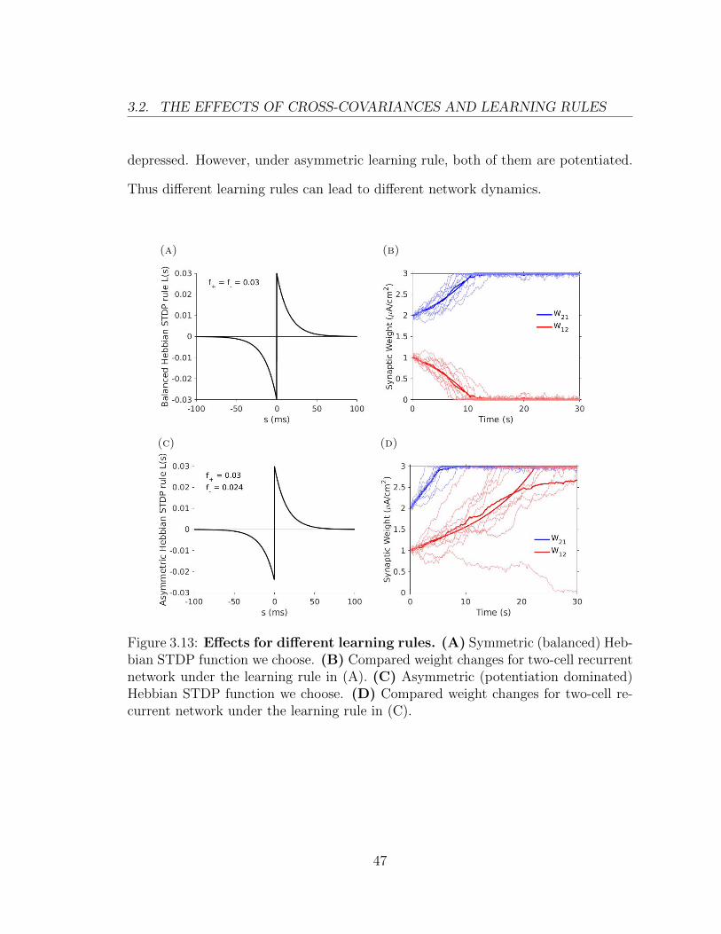
3.2. THE EFFECTS OF CROSS-COVARIANCES AND LEARNING RULES
depressed. However, under asymmetric learning rule, both of them are potentiated.
Thus different learning rules can lead to different network dynamics.
(a) (b)
(c) (d)
Figure 3.13: Effects for different learning rules. (A) Symmetric (balanced) Heb-bian STDP function we choose. (B) Compared weight changes for two-cell recurrentnetwork under the learning rule in (A). (C) Asymmetric (potentiation dominated)Hebbian STDP function we choose. (D) Compared weight changes for two-cell re-current network under the learning rule in (C).
47

3.2. THE EFFECTS OF CROSS-COVARIANCES AND LEARNING RULES
For a two-cell recurrent network, according to Eq.(2.6), the following system of
equations governs the evolution of the weights,
dW12
dt=´ +∞−∞ ∆W12(s)(C12(s) + r1r2)ds
dW21
dt=´ +∞−∞ ∆W21(s)(C21(s) + r2r1)ds
.
The phase planes for two-cell recurrent networks (like Figure 3.14) are obtained
using these equations. For an initial value of the weights (W12,W21), the related
phase plane shows what values will (W12,W21) attain under certain learning rule.
Here we follow the idea of Babadi and Abbott [4] in analyzing the phase planes.
(a) (b)
Figure 3.14: Phase planes for Figure 3.13. (A) Phase plane under balanced(symmetric) Hebbian STDP rule (Figure 3.13A). There are two stable fixed points,(3,0) and (0,3). (B) Phase plane under asymmetric Hebbian STDP rule (Figure3.13C). There are three stable fixed points, (3,0), (0,3) and (3,3).
48
3.2. THE EFFECTS OF CROSS-COVARIANCES AND LEARNING RULES
Here we set the upper bound of the synaptic weights at 3 (µA/cm2). Figure
3.14A shows the phase plane in the case of a balanced (symmetric) Hebbian STDP
rule while Figure 3.14B is for asymmetric learning rule. In the balanced case, there
are two stable fixed points (3,0) and (0,3), while the unstable fixed points are on the
diagonal line. Almost all initial weight values result in trajectories that are driven
to these two fixed points. In the asymmetric case, a new stable fixed point at (3,3)
emerges. For the parameters we chose, most initial weights will result in trajectories
that converge to this point. This explains the different dynamics of the weights un-
der these two leaning rule. Initially we set the weights (W12,W21) = (1, 2), under
symmetric learning rule, they will go to fixed point (0,3) (Figure 3.13B). However,
under asymmetric learning rule, they go to fixed point (3,3) (Figure 3.13D). This
implies that the asymmetric learning rule leads to a asymmetric final state, while
the symmetric learning rule leads to a symmetric final state.
We next illustrate the effects of the shapes of cross-covariances. We begin with the
case of unequal baseline firing rates for different networks. Here we apply asymmetric
Hebbian STDP rule on the two-cell recurrent networks. The cells from the two
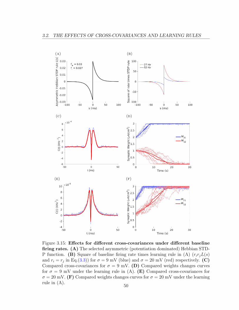
networks have the same µ value (µ=2 mV) but different levels of noise (σ=9 and 20
mV respectively). In this case, cells with σ=9 mV have baseline firing rate about 27
Hz, while cells with σ=20 mV have baseline firing rate about 52 Hz. The results are
shown in Figure 3.15 while the corresponding phase planes are in Figure 3.16.
49
3.2. THE EFFECTS OF CROSS-COVARIANCES AND LEARNING RULES
(a) (b)
(c)
-50 0 50t (ms)
-6
-4
-2
0
2
4
6
8
C(t
) (k
Hz
2)
#10 -4
(d)
(e) (f)
Figure 3.15: Effects for different cross-covariances under different baselinefiring rates. (A) The selected asymmetric (potentiation dominated) Hebbian STD-P function. (B) Square of baseline firing rate times learning rule in (A) (rirjL(s)and ri = rj in Eq.(3.3)) for σ = 9 mV (blue) and σ = 20 mV (red) respectively. (C)Compared cross-covariances for σ = 9 mV. (D) Compared weights changes curvesfor σ = 9 mV under the learning rule in (A). (E) Compared cross-covariances forσ = 20 mV. (F) Compared weights changes curves for σ = 20 mV under the learningrule in (A).
50

3.2. THE EFFECTS OF CROSS-COVARIANCES AND LEARNING RULES
Figure 3.15B shows that square of baseline firing rate times learning rule (rirjL(s)
and ri = rj in Eq.(3.3)) for σ = 9 mV (blue) and σ = 20 mV (red) respectively.
When the difference of the baseline firing rates is large, the difference of these prod-
ucts (rirjL(s)) is also large, as is the difference of the integrals of the products.
These difference will be reflected in the evolution of the synaptic weights. Figure
3.15C illustrates the case σ = 9 mV while Figure 3.15E shows the case σ = 20 mV.
Here we can see that the shape of the cross-covariance with higher sigma value is
broader under fixing µ value. Figure 3.15D and F are for the corresponding weights
changes curves. For the same learning rule, we have different dynamics for these
two networks: one weight is potentiated while another is depressed for lower σ value;
both of the weights are potentiated for higher σ value. Here the difference of network
dynamics is mainly due to the different baseline firing rates. We will show that we
can also get different network dynamics under same learning rule and fixed baseline
firing rate (Figure 3.20).
(a) (b) (c)
Figure 3.16: Phase planes related to Figure 3.15. (A) Phase plane for σ = 9mV under the learning rule in Figure 3.15A. (B) Phase plane for σ = 20 mV underthe learning rule in Figure 3.15A. (C) Phase plane for σ = 9 mV and µ = 3 mVunder the learning rule in Figure 3.15A.
51

3.2. THE EFFECTS OF CROSS-COVARIANCES AND LEARNING RULES
Figure 3.16A shows the phase plane when noise is smaller, that is σ = 9 mV,
while Figure 3.16B is for higher σ (σ = 20 mV) under the same asymmetric learning
rule. We can see that these two phase planes have the same stable fixed points (3,0),
(0,3) and (3,3). However, the region of initial weights which converge to the fixed
point (3,3) for bigger σ is much larger than that for smaller σ. Thus, under this same
asymmetric learning rule, the initial weights (W12,W21) = (1, 2) will go to the fixed
point (0,3) in the low σ case (Figure 3.15C), and to the fixed point (3,3) for higher
σ (Figure 3.15E). The main reason is the baseline firing rates. For µ = 2 mV and
σ = 9 mV, the baseline firing rate is about 27 Hz. It becomes to about 52 Hz for
µ = 2 mV and σ = 20 mV. In Figure 3.16C, we fix σ = 9 mV and increase µ from 2
mV to 3 mV. In this case, the baseline firing rate is about 52 Hz. We obtain a similar
phase plane as in Figure 3.16B. Increasing the baseline firing rate will increase the
basin of attraction for the fixed point (3,3).
We next use an analytical approach to understand these observations. Accord-
ing to Section 2.2, for simplification, we can rewrite the Hebbian STDP learning
(Eq.(2.2)) rule as
L(s) =
W0
ijH(Wmax −Wij)f+e− |s|τ+ , if s ≥ 0
W0ijH(Wij)(−f−)e
− |s|τ− , if s < 0
.
For the recurrent connected two cells i and j (i ↔ j), the two weights Wij and
52

3.2. THE EFFECTS OF CROSS-COVARIANCES AND LEARNING RULES
Wji always exist initially. So we have W0ij = W0
ji = 1. Then
L(s) =
H(Wmax −Wij)f+e
− sτ+ , if s ≥ 0
−H(Wij)f−esτ− , if s < 0
.
The theoretical weight changes due to the learning rule is
dWij
dt=
ˆ +∞
−∞L(s)(Cij(s) + rirj)ds (3.3)
=
ˆ +∞
−∞L(s)Cij(s)ds+ rirj
ˆ +∞
−∞L(s)ds
= f+
ˆ +∞
0
H(Wmax −Wij)e− sτ+ Cij(s)ds︸ ︷︷ ︸
A
− f−ˆ 0
−∞H(Wij)e
sτ−Cij(s)ds︸ ︷︷ ︸
B
+ rirj
ˆ +∞
−∞L(s)ds︸ ︷︷ ︸
C
= A−B + C .
3.2.1 Symmetric learning rules
For the symmetric (balanced) Hebbian STDP learning rule, that is when f+ = f−
and τ+ = τ− in Eq.(2.2), we have´ +∞−∞ L(s)ds = 0 and C = 0 in Eq.(3.3). In this
case, if Wij = Wji initially, we have Cij(s) = Cji(s) and both of them are sym-
metric with respect to the zero time axis (s = 0). Therefore, A = B anddWij
dt= 0
in Eq.(3.3), which implies that both synaptic weights will not change (See Figure
53
3.2. THE EFFECTS OF CROSS-COVARIANCES AND LEARNING RULES
3.14A where the diagonal consists of unstable fixed points). However, if the initial
synaptic weights are not equal, e.g. Wij > Wji, the amplitude of the peak of Cij(s)
in the positive time domain (potentiation side of the learning rule) will be larger
than that in the negative time domain (depression side of the learning rule). We
therefore obtain an asymmetric cross-covariance which drives the change in synaptic
weight for this case. In this case, A > B,dWij
dt> 0 in Eq.(3.3) and Wij increases
while Wji decreases (note Cji(s) = Cij(−s)). Therefore, larger initial weights are
potentiated and smaller initial weights depressed.
3.2.2 Asymmetric learning rules
We next consider one type of asymmetric learning rules, the potentiation dominat-
ed Hebbian STDP learning rules. The key difference between such rules and the
symmetric rules is that´ +∞−∞ L(s)ds > 0 and thus C > 0 in Eq.(3.3).
We can compute the term C explicitly.
C = rirj
[f+
ˆ +∞
0
H(Wmax −Wij)e− sτ+ ds− f−
ˆ 0
−∞H(Wij)e
sτ− ds
].
The learning rules modify the weights when 0 < Wij < Wmax, i.e. when
H(Wmax −Wij) = H(Wij) = 1. In this case,
C = rirj
(f+
ˆ +∞
0
e− sτ+ ds− f−
ˆ 0
−∞esτ− ds
)= rirj(f+τ+ − f−τ−) .
54
3.2. THE EFFECTS OF CROSS-COVARIANCES AND LEARNING RULES
Note that the magnitudes of cross-covariances we considered are around 10−4 ∼
10−3 (kHz2), while the baseline firing rates (ri, rj) are around 10 ∼ 20 (Hz). For the
learning rules such that
f+τ+ − f−τ− 6= 0 ,
we have
|C| � |A| and |C| � |B| .
If we choose a potentiation dominated Hebbian STDP learning rule by setting
f+ > f− and τ+ = τ− = τ in Eq.(2.2), for fixed baseline firing rates of all the neurons
(ri = rj = r) in the networks, we have
C = r2τ(f+ − f−) > 0 ,
and thus contribution from C in Eq.(3.3) is positive for all such networks.
When Wij = Wji, A > B for f+ > f−, even if both of Cij(s) and Cji(s) are
symmetric with respect to the zero time axis (s = 0). In addition, C > 0,dWij
dt> 0
and both of Wij and Wji will be potentiated. This implies that (Wmax,Wmax) is a
fixed point (Figure 3.14B).
When the two weights are not equal, the larger will be potentiated. The smaller
one, if the difference between it and the bigger one is not large (the cross-covariances
does not change much compared to the case of equal synaptic weights), we may
55
3.2. THE EFFECTS OF CROSS-COVARIANCES AND LEARNING RULES
have A − B + C > 0 for f+ > f− and C > 0. In this case, the weaker synaptic
weight also gets potentiated. With fixed neuron properties (σ and µ), the basin of
attraction of the stable fixed point (Wmax,Wmax) in the phase plane is determined
by the difference between f+ and f−. The larger this difference, the larger the basin
of attraction.
If we fix the potentiation dominated learning rule and increase the baseline firing
rates of both cells (ri and rj) by increasing σ or µ, part C can increase dramatically,
and make a larger contribution, or even dominate in Eq.(3.3). Both of the initial
weights will be potentiated due to the high positive C value. This leads to the
increase of the basin of attraction for the stable fixed point (Wmax,Wmax) in the
phase plane (Figure 3.16).
We can also build the potentiation dominated Hebbian STDP learning rules by
setting f+ = f− = f and τ+ > τ− in Eq.(2.2). In this case, for fixed baseline firing
rate (r) of all the neurons in the networks, we have
C = r2f(τ+ − τ−) > 0
is also a positive constant.
With a fixed baseline firing rate, the cross-covariances between neurons will not
change much when varying µ and σ (for fixed weights between neurons). The changes
in cross-covariances will change the values of A and B a bit. However, comparing
with the high positive constant C, such changes are very small and affect the phase
planes of the weights only a little. This means the basin of attraction in the phase
56

3.2. THE EFFECTS OF CROSS-COVARIANCES AND LEARNING RULES
planes are mainly determined by the C value for such potentiation dominated learn-
ing rules (Figure 3.17).
Figure 3.17: Phase planes for small differences between τ+ and τ−.
The different rows of Figure 3.17 show that phase planes change little when
we vary µ and σ (change the cross-covariances). The small differences are in the
boundaries of different basins of attraction.
57
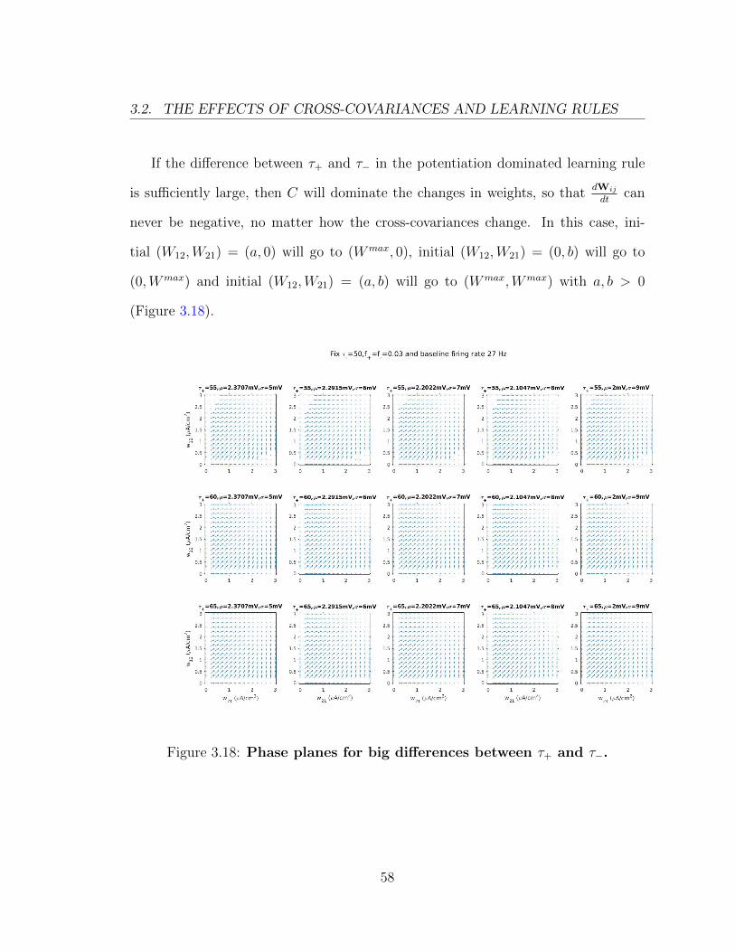
3.2. THE EFFECTS OF CROSS-COVARIANCES AND LEARNING RULES
If the difference between τ+ and τ− in the potentiation dominated learning rule
is sufficiently large, then C will dominate the changes in weights, so thatdWij
dtcan
never be negative, no matter how the cross-covariances change. In this case, ini-
tial (W12,W21) = (a, 0) will go to (Wmax, 0), initial (W12,W21) = (0, b) will go to
(0,Wmax) and initial (W12,W21) = (a, b) will go to (Wmax,Wmax) with a, b > 0
(Figure 3.18).
Figure 3.18: Phase planes for big differences between τ+ and τ−.
58
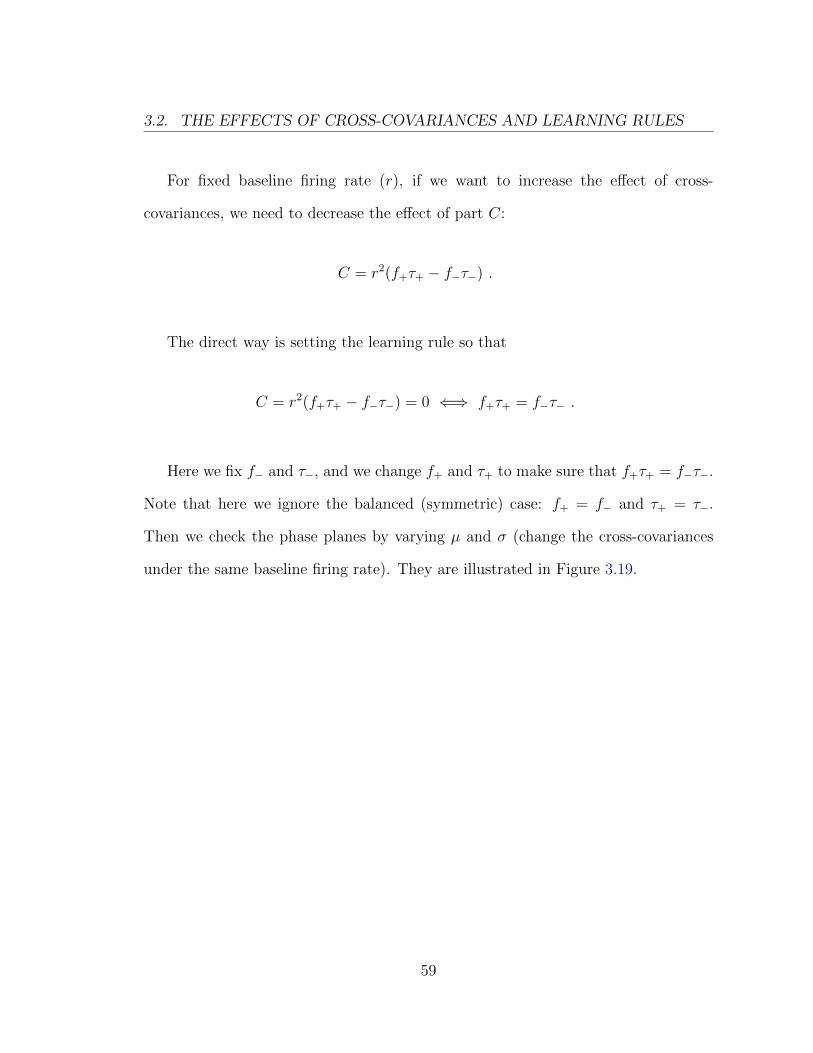
3.2. THE EFFECTS OF CROSS-COVARIANCES AND LEARNING RULES
For fixed baseline firing rate (r), if we want to increase the effect of cross-
covariances, we need to decrease the effect of part C:
C = r2(f+τ+ − f−τ−) .
The direct way is setting the learning rule so that
C = r2(f+τ+ − f−τ−) = 0 ⇐⇒ f+τ+ = f−τ− .
Here we fix f− and τ−, and we change f+ and τ+ to make sure that f+τ+ = f−τ−.
Note that here we ignore the balanced (symmetric) case: f+ = f− and τ+ = τ−.
Then we check the phase planes by varying µ and σ (change the cross-covariances
under the same baseline firing rate). They are illustrated in Figure 3.19.
59

3.2. THE EFFECTS OF CROSS-COVARIANCES AND LEARNING RULES
Figure 3.19: Phase planes for setting the integral of learning rule to be 0.
From the middle and bottom rows of Figure 3.19, the changes in the phase planes
are much more obvious. This implies the effect of cross-covariances is larger. Here
we use the the parameters of bottom row left one and right one of Figure 3.19 as an
example (Figure 3.20), which shows that cross-covariances can change the network
dynamics for fixed baseline firing rate under such learning rules. We can see that
the properties of the cells (µ and σ) can affect the cross-covariances, and therefor
can affect the dynamics of the weights in the network. However, this only happens
when the term C is not big compared with A and B in Eq.(3.3).
60

3.2. THE EFFECTS OF CROSS-COVARIANCES AND LEARNING RULES
(a) (b)
(c) (d)
Figure 3.20: Cross-covariances can affect network dynamics for the samebaseline firing rate. (A) Selected learning rule with the parameter in Figure 3.19.(B) Theoretical weights changes for σ = 5 mV and σ = 9 mV under the learning rulein (A) respectively. (C) Compared weights changes for σ = 5 mV. (D) Comparedweights changes for σ = 9 mV.
61

CHAPTER 4
Results for larger networks
In the previous section, we studied how STDP together with the properties of spike
train cross-covariances determine the evolution of synaptic weights in networks of
two neurons. In this chapter we will generalize these ideas, and examine the evolu-
tion of weights in larger networks. For demonstration we simulate networks of put
to 100 EIF neurons, although our conclusions and approach hold more generally.
62

4.1. DIFFERENT µ-σ SETTINGS HAVE DIFFERENT WEIGHTCHANGE SPEEDS
4.1 Different µ-σ settings have different weight
change speeds
In Section 3.2, we showed that, with a fixed baseline firing rate and with a balanced
STDP learning rule, for two coupled neurons with different levels of drive (µ) and
background noise (σ), the synaptic weights can change at different rates. Similar
results hold in larger networks, and we have consequences for their global connectivity
structure.
The different intrinsic properties of the cells (µ-σ settings) affect the cross-
covariances between the spike trains of synaptically connected pairs of cells in the net-
work (See Figure 3.10). This in turn leads to distinct dynamics of synaptic weights,
as governed by the learning rule. Here we choose µ-σ settings shown in Table 2.1.
The cross-covariances of two-cell recurrent networks for these 5 different parameter
values are shown in the following Figure 4.1A. We also show the balanced Hebbian
STDP learning rule we use in the simulations (Figure 4.1B; By “balanced” we again
mean that f+ = f− and τ+ = τ− in Eq.(2.2)). Note that the baseline firing rates in
Figure 3.10 (about 27 Hz) and 4.1A (about 7.6 Hz) are different. We can see that
there are more oscillations for higher baseline firing rates case.
63
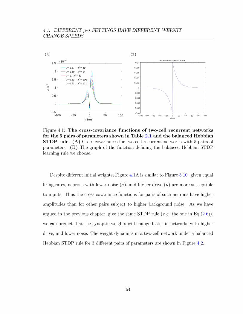
4.1. DIFFERENT µ-σ SETTINGS HAVE DIFFERENT WEIGHTCHANGE SPEEDS
(a)
-100 -50 0 50 100= (ms)
-0.5
0
0.5
1
1.5
2
2.5
kHz
2
#10 -4
7= 1.37, <2= 49
7= 1.19, <2= 64
7= 1, <2= 81
7= 0.81, <2= 100
7= 0.61, <2= 121
(b)
−100 −80 −60 −40 −20 0 20 40 60 80 100−0.01
−0.008
−0.006
−0.004
−0.002
0
0.002
0.004
0.006
0.008
0.01
τ (ms)
Balanced Hebbian STDP rule
Figure 4.1: The cross-covariance functions of two-cell recurrent networksfor the 5 pairs of parameters shown in Table 2.1 and the balanced HebbianSTDP rule. (A) Cross-covariances for two-cell recurrent networks with 5 pairs ofparameters. (B) The graph of the function defining the balanced Hebbian STDPlearning rule we choose.
Despite different initial weights, Figure 4.1A is similar to Figure 3.10: given equal
firing rates, neurons with lower noise (σ), and higher drive (µ) are more susceptible
to inputs. Thus the cross-covariance functions for pairs of such neurons have higher
amplitudes than for other pairs subject to higher background noise. As we have
argued in the previous chapter, give the same STDP rule (e.g. the one in Eq.(2.6)),
we can predict that the synaptic weights will change faster in networks with higher
drive, and lower noise. The weight dynamics in a two-cell network under a balanced
Hebbian STDP rule for 3 different pairs of parameters are shown in Figure 4.2.
64

4.1. DIFFERENT µ-σ SETTINGS HAVE DIFFERENT WEIGHTCHANGE SPEEDS
Figure 4.2: The evolution of synaptic weights for three different pairs ofparameter values specifying intrinsic properties of cells. Results are obtainedusing the theory developed in Section 2.3.
As in Figure 3.11A, we can see that the synaptic weights in the less noisy networks
(with lower σ) reach the boundaries faster (See Figure 4.2).
We next built a network of ten all–to–all connected cells. We again used the
five different parameter sets described above, and let the synaptic weights in the
network evolve according to the same balanced Hebbian STDP rule describe above.
We used the same initial synaptic weight matrix for all these networks (Figure 4.3A),
and obtained the same steady state (Figure 4.3B) after a transient period. Here the
initial synaptic weight matrix is generated randomly. The dynamics of synaptic
weights for 3 parameter sets are shown in Figure 4.4.
65

4.1. DIFFERENT µ-σ SETTINGS HAVE DIFFERENT WEIGHTCHANGE SPEEDS
(a)
Initial synaptic weight matrix
2 4 6 8 10
1
2
3
4
5
6
7
8
9
100
0.1
0.2
0.3
0.4
0.5
(b)
Theoretical final state
2 4 6 8 10
1
2
3
4
5
6
7
8
9
100
0.1
0.2
0.3
0.4
0.5
Figure 4.3: The initial synaptic weight matrix and the theoretical steadystate for all the 5 µ-σ pairs. (A) The initial synaptic weight matrix. (B) Thetheoretical steady state of the weight matrix after learning. This final state is thesame for each of the five parameter settings we used.
(a) (b) (c)
Figure 4.4: The evolution of synaptic weights for three different parametersettings. (A) The dynamics of the synaptic weights obtained using the theorydeveloped in Section 2.3. (B) The dynamics of the synaptic weights for the sameparameter values as in (A) obtained by direct simulation of the network and averagingover 10 realizations. (C) The comparison between the dynamics of the synapticweights obtained by theory ((A)) and simulation ((B)). The thick curves are from(A) while the thin curves are from (B).
66
4.2. WEIGHT DYNAMICS DEPEND ON INDIVIDUALNEURON PROPERTIES
In this example the main effect of the different parameter settings is the speed at
which the final state is reached. Networks with less background noise (lower σ) reach
the final state faster than those with higher levels of noise, but the same baseline
firing rate. This verifies our prediction and generalizes our results in Section 3.2.
4.2 Weight dynamics depend on individual
neuron properties
As discussed in Section 3.1.2 (Figure 3.7), we know that, for the same baseline firing
rate, different properties of individual cells, i.e different values of the parameters µ
and σ, in a two-cell recurrent network affect spike train cross-covariances. In Sec-
tion 3.2, we can show that learning rules can magnify the effect of cross-covariances
on weight change dynamics. Here we will examine how these two factors affect the
dynamics of synaptic weight changes in larger networks.
4.2.1 Balanced Hebbian STDP case
As in the previous section we examine weight changes under a balanced Hebbian
STDP rule. As we have shown in Section 3.2 this implies that the cross-covariances
dominate the evolution of synaptic weights. We begin by analyzing the phase planes
(vector fields) of two-cell, recurrent networks with each neuron with different parame-
ter settings. We will then use the properties found in two-cell networks to understand
67
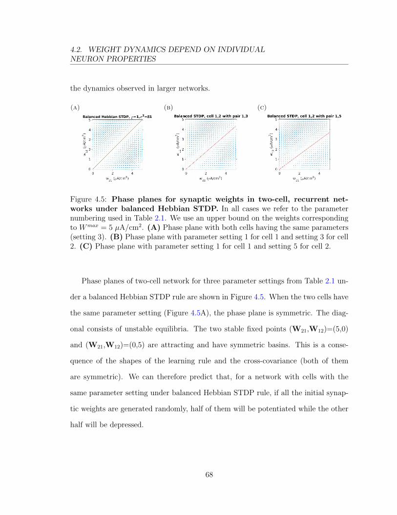
4.2. WEIGHT DYNAMICS DEPEND ON INDIVIDUALNEURON PROPERTIES
the dynamics observed in larger networks.
(a) (b) (c)
Figure 4.5: Phase planes for synaptic weights in two-cell, recurrent net-works under balanced Hebbian STDP. In all cases we refer to the parameternumbering used in Table 2.1. We use an upper bound on the weights correspondingto Wmax = 5 µA/cm2. (A) Phase plane with both cells having the same parameters(setting 3). (B) Phase plane with parameter setting 1 for cell 1 and setting 3 for cell2. (C) Phase plane with parameter setting 1 for cell 1 and setting 5 for cell 2.
Phase planes of two-cell network for three parameter settings from Table 2.1 un-
der a balanced Hebbian STDP rule are shown in Figure 4.5. When the two cells have
the same parameter setting (Figure 4.5A), the phase plane is symmetric. The diag-
onal consists of unstable equilibria. The two stable fixed points (W21,W12)=(5,0)
and (W21,W12)=(0,5) are attracting and have symmetric basins. This is a conse-
quence of the shapes of the learning rule and the cross-covariance (both of them
are symmetric). We can therefore predict that, for a network with cells with the
same parameter setting under balanced Hebbian STDP rule, if all the initial synap-
tic weights are generated randomly, half of them will be potentiated while the other
half will be depressed.
68

4.2. WEIGHT DYNAMICS DEPEND ON INDIVIDUALNEURON PROPERTIES
When we consider a network of two cells with different parameter settings (Figure
4.5B and C) this symmetry is broken. The line of unstable fixed points is tilted toward
the axis corresponding to the weight of the connection from the cell with higher drive
(µ) to the cell with higher noise (σ). This implies that the basin of attraction of the
fixed point (W21,W12)=(0,5) is larger than the basin of (W21,W12)=(5,0). The
outgoing synapses of the neuron with higher noise values (parameter settings 3 and
5 in Table 2.1) are more likely to be potentiated, while the incoming synapses are
likely to weaken. Conversely, outgoing synapses from the neuron with higher drive
value (setting 1 in Table 2.1) are more likely to weaken and its incoming synapses
are more likely to be potentiated.
We therefore predict that for a network consisting of different groups of cells
sharing the same initial baseline firing rate, but with different individual properties,
under balanced Hebbian STDP rule, the synaptic weights of the connections from
cells with lower drive (lower µ) and higher noise (higher σ) to cells with higher drive
and lower noise will be potentiated. The synaptic weights of the connections from
cells with higher drive to those with lower drive will weaken. These synapses can
eventually be pruned if the lower bound is set to 0.
We next examine the dynamics of synaptic weights in a network of 100 cells with
all–to–all connectivity. We again use a balanced Hebbian STDP rule. The network
consists of two groups composed of cells with indices 1-50 (Group 1), and 51-100
(Group 2), respectively. Cells in the two groups have the same baseline firing rates,
and share the same intrinsic properties with those within the group, but not with
those in the different group. That is the values of the parameters µ and σ differ
69

4.2. WEIGHT DYNAMICS DEPEND ON INDIVIDUALNEURON PROPERTIES
between the two groups. As a result we can split the synaptic weight matrix into
four quarters corresponding to connections within and between these two groups.
We will use two examples to illustrate how our phase plan analysis can be used to
predict weight dynamics in a larger network.
Example 4.2.1. We use parameter set 3 for cells in the Group 1 (indices 1-50),
and set 1 for cells in Group 2 (indices 51-100). The initial synaptic weight matrix is
generated randomly, and it is shown in Figure 4.6.
Initial synaptic weight matrix
20 40 60 80 100
10
20
30
40
50
60
70
80
90
100 0
0.005
0.01
0.015
0.02
0.025
0.03
0.035
0.04
0.045
0.05
Figure 4.6: The initial synaptic weight matrix of 100-cell dense network.
The final state of the synaptic weights in the network is shown in Figure 4.7
obtained both using our theoretical approach, and direct simulations of the network
of EIF neurons. The two approaches give quantitatively similar results. As predicted
by our simulation of the two cell recurrent network, the bottom-left quarter (the
weights corresponding to connections from higher noise neurons (parameter set 3)
to lower noise neurons (parameter set 1)), is lighter than the top-right quarter after
training. This indicates that these weights are bigger. We quantify this effect further
below. The comparison of weight dynamics is in Figure 4.8.
70
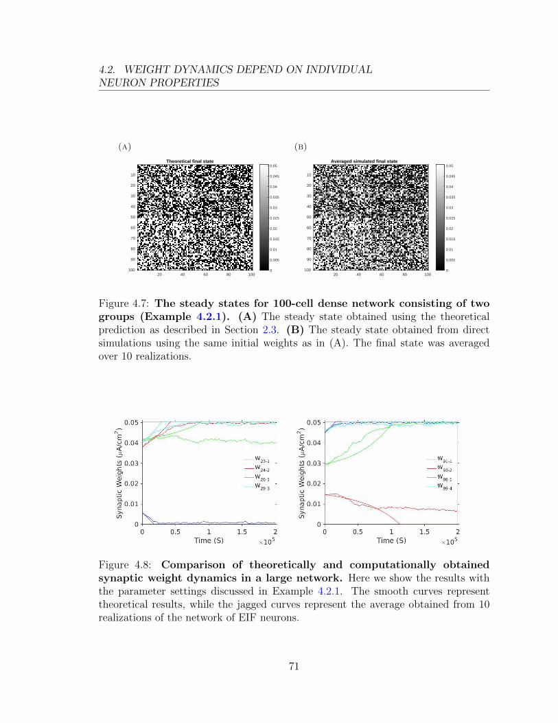
4.2. WEIGHT DYNAMICS DEPEND ON INDIVIDUALNEURON PROPERTIES
(a)
Theoretical final state
20 40 60 80 100
10
20
30
40
50
60
70
80
90
100 0
0.005
0.01
0.015
0.02
0.025
0.03
0.035
0.04
0.045
0.05
(b)
Averaged simulated final state
20 40 60 80 100
10
20
30
40
50
60
70
80
90
100 0
0.005
0.01
0.015
0.02
0.025
0.03
0.035
0.04
0.045
0.05
Figure 4.7: The steady states for 100-cell dense network consisting of twogroups (Example 4.2.1). (A) The steady state obtained using the theoreticalprediction as described in Section 2.3. (B) The steady state obtained from directsimulations using the same initial weights as in (A). The final state was averagedover 10 realizations.
Figure 4.8: Comparison of theoretically and computationally obtainedsynaptic weight dynamics in a large network. Here we show the results withthe parameter settings discussed in Example 4.2.1. The smooth curves representtheoretical results, while the jagged curves represent the average obtained from 10realizations of the network of EIF neurons.
71

4.2. WEIGHT DYNAMICS DEPEND ON INDIVIDUALNEURON PROPERTIES
To quantify this difference we compute the mean synaptic weight for each of the
four types of connections between and within the groups in the final state of the
network. These are shown in Table 4.1 with the standard error of the averaged sim-
ulated final states obtain using bootstrap statistics (boot() function in R with 1000
replicates).
group 1: pair 3(strong noise) mean weights(µA/cm2)standard error
group 2: pair 1(weak noise) theory simulationstrong-strong(top-left) 0.025 0.025 0.00039weak-strong(top-right) 0.020 0.020 0.00040
strong-weak(bottom-left) 0.030 0.030 0.00039weak-weak(bottom-right) 0.025 0.025 0.00040
Table 4.1: The mean weights in each of the four quarters of the synaptic weightsmatrix for Example 4.2.1.
We again observe that the mean synaptic weight for the strong-weak (noise level)
connections (bottom-left quarter of the synaptic weight matrix) is higher than that
for weak-strong connections (top-right quarter) for both theoretical and simulated
final states. The mean weights for strong-strong (top-left quarter) connections and
weak-weak connections(bottom-right quarter) are very close. Moreover, the theory
and simulation results agree closely.
72
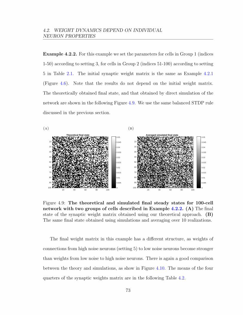
4.2. WEIGHT DYNAMICS DEPEND ON INDIVIDUALNEURON PROPERTIES
Example 4.2.2. For this example we set the parameters for cells in Group 1 (indices
1-50) according to setting 3, for cells in Group 2 (indices 51-100) according to setting
5 in Table 2.1. The initial synaptic weight matrix is the same as Example 4.2.1
(Figure 4.6). Note that the results do not depend on the initial weight matrix.
The theoretically obtained final state, and that obtained by direct simulation of the
network are shown in the following Figure 4.9. We use the same balanced STDP rule
discussed in the previous section.
(a)
Theoretical final state
20 40 60 80 100
10
20
30
40
50
60
70
80
90
100 0
0.005
0.01
0.015
0.02
0.025
0.03
0.035
0.04
0.045
0.05
(b)
Averaged simulated final state
20 40 60 80 100
10
20
30
40
50
60
70
80
90
100 0
0.005
0.01
0.015
0.02
0.025
0.03
0.035
0.04
0.045
0.05
Figure 4.9: The theoretical and simulated final steady states for 100-cellnetwork with two groups of cells described in Example 4.2.2. (A) The finalstate of the synaptic weight matrix obtained using our theoretical approach. (B)The same final state obtained using simulations and averaging over 10 realizations.
The final weight matrix in this example has a different structure, as weights of
connections from high noise neurons (setting 5) to low noise neurons become stronger
than weights from low noise to high noise neurons. There is again a good comparison
between the theory and simulations, as show in Figure 4.10. The means of the four
quarters of the synaptic weights matrix are in the following Table 4.2.
73

4.2. WEIGHT DYNAMICS DEPEND ON INDIVIDUALNEURON PROPERTIES
Figure 4.10: The comparison of the evolution of selected weights in a 100-cell network of all–to–all coupled cells with parameter setting as discussedin Example 4.2.2. Smooth curves are theoretical results, while jagged curvesrepresent the average over 10 realizations.
group 1: pair 3(weak noise) mean weights(µA/cm2)standard error
group 2: pair 5(strong noise) theory simulationweak-weak(top-left) 0.025 0.025 0.00041
strong-weak(top-right) 0.030 0.030 0.00040weak-strong(bottom-left) 0.020 0.020 0.00039
strong-strong(bottom-right) 0.025 0.025 0.00041
Table 4.2: The mean weights in each of the four quarters of the synaptic weightsmatrix for Example 4.2.2.
Here we show that the mean weight of connections from neurons with strong
background noise to those with weak niose (strong-weak, top-right quarter) is higher
than that of weak-strong connections (bottom-left quarter), both in the case of the
final state obtained theoretically and by simulations. The mean weights of weak-weak
connections (top-left quarter) and strong-strong connections (bottom-right quarter)
74

4.2. WEIGHT DYNAMICS DEPEND ON INDIVIDUALNEURON PROPERTIES
are in the same level. Moreover, all the theoretical mean weights are close to their
related simulated ones.
These two examples agree with the conclusions of our two-cell, recurrent network
in the beginning of this section : the synaptic weights of the connections from cells
with lower drive (lower µ) and higher internal noise (higher σ) to those with high-
er drive (higher µ) and lower lower internal noise( lower σ) are potentiated, while
weights in the opposite direction are typically weakened under a balanced Hebbian
STDP rule. This is due to the difference in the size of basins of attraction of the
fixed points for the two different types of cells.
4.2.2 Balanced Anti-Hebbian STDP case
Here we ask what is the effect of a balanced Anti-Hebbian STDP rule mentioned
in Section 2.2 on the evolution of synaptic weights in larger networks. This rule is
defined by the following weight change function:
∆Wji(s) =
W0
jiH(Wji)L(s) , if s ≥ 0
W0jiH(Wmax −Wji)L(s) , if s < 0
,
where
L(s) =
−f−e
− |s|τ+ , if s ≥ 0
f+e− |s|τ− , if s < 0
.
75

4.2. WEIGHT DYNAMICS DEPEND ON INDIVIDUALNEURON PROPERTIES
The rule is similar to the Hebbian STDP rule defined in Eq.(2.2), but it reverses
the windows of potentiation and depression. As with the the balanced Hebbian
STDP rule, this rule also leads to a cancellation of part C in Eq.(3.3) so that the
cross-covariances control the weight evolution.
Similar as the balanced Hebbian case, fixing the learning rule as balanced Anti-
Hebbian STDP rule, we study the phase planes for two-cell recurrent networks with
each neuron in different parameter (µ-σ) settings firstly.
Phase planes of two-cell network for three parameter settings from Table 2.1 un-
der a balanced Anti-Hebbian STDP rule are shown in Figure 4.11.
(a) (b) (c)
Figure 4.11: Phase planes for synaptic weights in two-cell, recurrent net-work under balanced Anti-Hebbian STDP rule. In all cases we refer to theparameter numbering used in Table 2.1. We use an upper bound on the weightscorresponding to Wmax = 5 µA/cm2. (A) Phase plane with both cells having thesame parameters (setting 3). (B) Phase plane with parameter setting 1 for cell 1and setting 3 for cell 2. (C) Phase plane with parameter setting 1 for cell 1 andsetting 5 for cell 2.
76
4.2. WEIGHT DYNAMICS DEPEND ON INDIVIDUALNEURON PROPERTIES
Since the Anti-Hebbian STDP rule differs from the Hebbian STDP rule in the
that potentiation side and depression side are reversed, we obtain the same phase
planes as Figure 4.5, but with reversed time flow. This means that all arrows are
now reversed (see Figure 4.11), and therefore all initial conditions converge to the
line of fixed points.
For the two cells with the same parameter (µ-σ) setting (Figure 4.11A), the phase
plane is also symmetric. We can make a prediction that, for a network with cells
of the same parameter setting, under balanced Anti-Hebbian STDP rule, if all the
initial weights are generated randomly, they will attain the same value or similar
values finally.
Additionally, for the two cells with different parameter settings (Figure 4.11B and
C), the line of equilibrium (stable fixed points) is tilted toward the axis corresponding
to the weight of the connection from the cell with higher drive (µ) to the cell with
higher noise (σ). This implies that the outgoing synapses of the neuron with higher
noise (parameter settings 3 and 5 in Table 2.1) are more likely to weaken, while its
incoming synapses are likely to be potentiated. Conversely, outgoing synapses from
the neuron with higher drive (setting 1 in Table 2.1) are more likely to be potentiated
and its incoming synapses are more likely to weaken.
As in the previous section we can use these observations to examine the evolution
of synaptic weights in networks composed of different groups of cells with the same
baseline firing rates, but different levels of drive and noise. Under a balanced Anti-
Hebbian STDP rule, the weights of synaptic connections from cells with higher noise
to those with lower noise will weaken. The weights going of synapses in the opposite
77

4.2. WEIGHT DYNAMICS DEPEND ON INDIVIDUALNEURON PROPERTIES
direction will be potentiated. We verify this prediction in the following example.
Example 4.2.3. For this example we set the parameters for cells in Group 1 (indices
1-50) according to setting 1, for cells in Group 2 (indices 51-100) according to setting 5
in Table 2.1. The initial synaptic weight matrix is the same as previous two examples
(Figure 4.6). Under balanced Anti-Hebbian STDP rule, the theoretically obtained
final state, and that obtained by direct simulation of the network are shown in the
following Figure 4.12.
(a)
Theoretical final state
20 40 60 80 100
10
20
30
40
50
60
70
80
90
100 0
0.005
0.01
0.015
0.02
0.025
0.03
0.035
0.04
0.045
0.05
(b)
Averaged simulated final state
20 40 60 80 100
10
20
30
40
50
60
70
80
90
100 0
0.005
0.01
0.015
0.02
0.025
0.03
0.035
0.04
0.045
0.05
Figure 4.12: The theoretical and simulated final steady states for 100-cellnetwork with two groups of cells described in Example 4.2.3. (A) The finalstate of the synaptic weight matrix obtained using our theoretical approach. (B)The same final state obtained using simulations and averaging over 10 realizations.
We can see that, the final weight matrix in this example has a different structure,
as weights of connections from lower noise neurons to higher noise neurons (bottom-
left quarter) become stronger than weights from higher noise to lower noise neurons
(top-right quarter). The results look similar as Example 4.2.1, but with reversed
78

4.2. WEIGHT DYNAMICS DEPEND ON INDIVIDUALNEURON PROPERTIES
parameter (µ-σ) settings according to the reversed sides of potentiation and depres-
sion in the learning rules. There is again a good comparison between the theory and
simulations, as show in Figure 4.13. The means of the four quarters of the synaptic
weights matrix are in the following Table 4.3.
Figure 4.13: The comparison of the evolution of selected weights in a 100-cell network of all–to–all coupled cells with parameter setting as discussedin Example 4.2.3. Smooth curves are theoretical results, while jagged curvesrepresent the average over 10 realizations.
group 1: pair 1(weak noise) mean weights(µA/cm2)standard error
group 2: pair 5(strong noise) theory simulationweak-weak(top-left) 0.025 0.025 0.00022
strong-weak(top-right) 0.020 0.020 0.00019weak-strong(bottom-left) 0.028 0.028 0.00023
strong-strong(bottom-right) 0.025 0.025 0.00022
Table 4.3: The mean weights in each of the four quarters of the synaptic weightsmatrix for Example 4.2.3.
Here we show that the mean weight of connections from neurons with strong
background noise to those with weak niose (strong-weak, top-right quarter) is lower
79
4.3. INTERNAL CELL PROPERTIES CAN LEAD TO DIFFERENCES INSYNAPTIC WEIGHT EVOLUTION
than that of weak-strong connections (bottom-left quarter), both in the case of the
final state obtained theoretically and by simulations. The mean weights of weak-weak
connections (top-left quarter) and strong-strong connections (bottom-right quarter)
are in the same level. Moreover, all the theoretical mean weights are close to their
related simulated ones.
This example demonstrates that, under balanced Anti-Hebbian STDP rules,
weights of connection from cells with higher internal noise (σ) to those with lower
noise will weaken, while weights of connections in the opposite direction are poten-
tiated. This agrees with our predictions.
4.3 Internal cell properties can lead to differences
in synaptic weight evolution
We next consider a network of neurons with the same parameter setting µ-σ, and
therefore the same baseline firing rates. We then compare the dynamics of synaptic
weights for different parameter settings, but same baseline firing rates. We use the
potentiation dominated Hebbian STDP rule and set f+ = A · f− and τ+ = τ− with
A > 1. Again, our network initially has all–to–all connectivity. In this case, the
term denoted by C in Eq.(3.3) is bigger than 0, and hence firing rates will affect the
weight change in addition to the effect of cross-covariances. We will show that, the
cross-covariances can still affect the evolution of the synaptic weights in this case.
80

4.3. INTERNAL CELL PROPERTIES CAN LEAD TO DIFFERENCES INSYNAPTIC WEIGHT EVOLUTION
As in the previous sections, we start by analyzing the phase planes for two-cell
networks first. These are shown for parameter settings 1 and 5, under potentiation
dominated Hebbian STDP with A = 1.5 in Figure 4.14.
(a) (b)
Figure 4.14: The phase planes of synaptic weights in a two-cell, recurrentnetwork under a potentiation dominated STDP rule. (A) Phase plane forthe parameter setting 1. (B) Phase plane for the parameter setting 5.
The phase planes show that, in this case there are three fixed points: (W21,W12)=(5,0),
(0,5) and (5,5). All thee fixed points are stable. However, the basin of attraction of
the stable fixed point corresponding to equal final weights, (W21,W12) = (5, 5) is
larger for parameter setting 5 than for setting 1. Thus, we can predict that networks
of identical cells with higher noise (σ) under potentiation dominated Hebbian STDP
rule will exhibit more recurrent connections – and more connections overall – after
in the final state. We illustrate that this conclusion holds in the following examples.
81

4.3. INTERNAL CELL PROPERTIES CAN LEAD TO DIFFERENCES INSYNAPTIC WEIGHT EVOLUTION
Example 4.3.1. We use the potentiation dominated Hebbian STDP rule (f+ =
1.05 · f− and τ+ = τ−), and we begin with a small network of 10 all–to–all connected
cells for direct observation. We will show the results hold for large networks (networks
of 100 all–to–all connected cells, Example 4.3.3). We want to examine networks of
cells with different internal properties (parameter settings). The initial synaptic
weight matrix is fixed for all networks here, which is shown in Figure 4.3A. For the
networks of neurons with parameter setting 1 and 5, the theoretically obtained final
states, and those obtained by direct simulation are shown in the following Figure
4.15
Figure 4.15 shows that, after training, there are more white blocks in the synaptic
weight matrices of the second row. This means, there are more potentiated weights
in the network of neurons with parameter setting 5 than those for parameter setting
1. Therefore the network of cells with higher noise (parameter setting 5) get more
recurrently connected cells. There is also a good comparison between the theory and
simulations, as show in Figure 4.16.
82
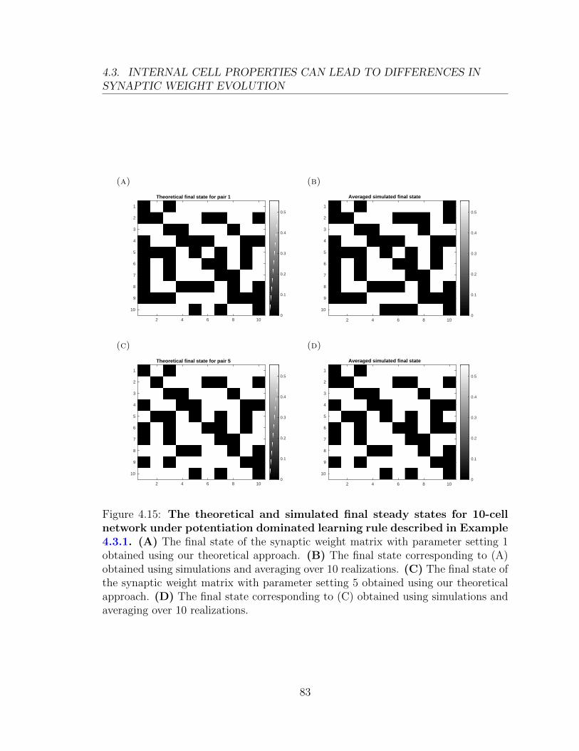
4.3. INTERNAL CELL PROPERTIES CAN LEAD TO DIFFERENCES INSYNAPTIC WEIGHT EVOLUTION
(a)
Theoretical final state for pair 1
2 4 6 8 10
1
2
3
4
5
6
7
8
9
100
0.1
0.2
0.3
0.4
0.5
(b)
Averaged simulated final state
2 4 6 8 10
1
2
3
4
5
6
7
8
9
100
0.1
0.2
0.3
0.4
0.5
(c)
Theoretical final state for pair 5
2 4 6 8 10
1
2
3
4
5
6
7
8
9
100
0.1
0.2
0.3
0.4
0.5
(d)
Averaged simulated final state
2 4 6 8 10
1
2
3
4
5
6
7
8
9
100
0.1
0.2
0.3
0.4
0.5
Figure 4.15: The theoretical and simulated final steady states for 10-cellnetwork under potentiation dominated learning rule described in Example4.3.1. (A) The final state of the synaptic weight matrix with parameter setting 1obtained using our theoretical approach. (B) The final state corresponding to (A)obtained using simulations and averaging over 10 realizations. (C) The final state ofthe synaptic weight matrix with parameter setting 5 obtained using our theoreticalapproach. (D) The final state corresponding to (C) obtained using simulations andaveraging over 10 realizations.
83

4.3. INTERNAL CELL PROPERTIES CAN LEAD TO DIFFERENCES INSYNAPTIC WEIGHT EVOLUTION
(a)
Time (S) #10 4
0 5 10 15
Syn
aptic
Wei
ghts
(m
V)
0
0.1
0.2
0.3
0.4
0.5
Match figure 4
W96
W910
W104
W109
(b)
Time (S) #10 4
0 5 10 15
Syn
aptic
Wei
ghts
(m
V)
0
0.1
0.2
0.3
0.4
0.5
Match figure 3
W67
W74
W79
W82
Figure 4.16: The comparison of the evolution of selected weights in a 10-cellnetwork of all–to–all coupled cells with parameter setting as discussed inExample 4.3.1. Smooth curves are theoretical results, while jagged curves representthe average over 10 realizations. (A) For network of identical cells with parametersetting 1. (B) For network of identical cells with parameter setting 5.
Example 4.3.2. Here we use the potentiation dominated Hebbian STDP rule by
setting f+ = 1.05 · f−, and again, τ+ = τ−. Then we apply the rule on the same
network of 10 all–to–all connected cells as Example 4.3.1. For the networks of neurons
with parameter setting 1 and 5, the theoretically obtained final states, and those
obtained by direct simulation are shown in the following Figure 4.17 and Figure 4.18
respectively, together with comparison of the evolution of selected weights between
the theory and simulations.
84
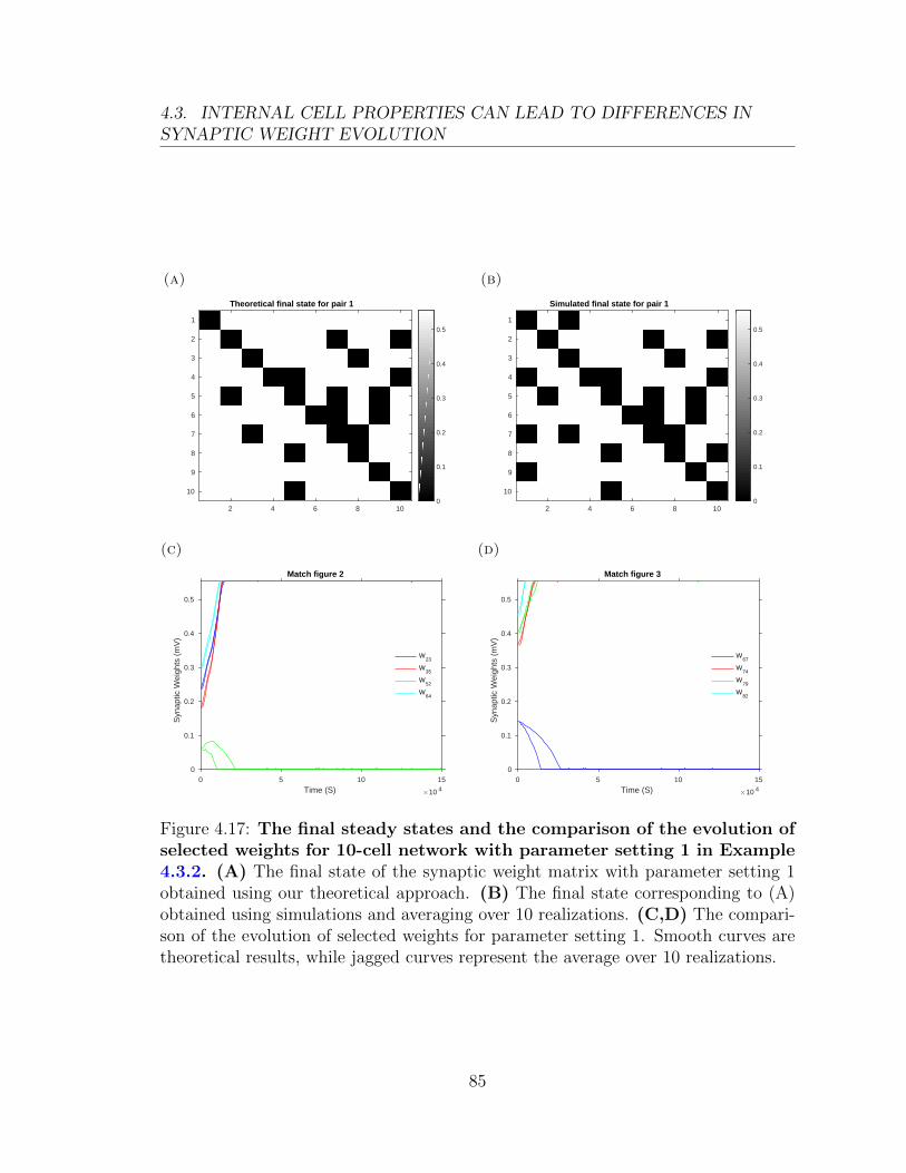
4.3. INTERNAL CELL PROPERTIES CAN LEAD TO DIFFERENCES INSYNAPTIC WEIGHT EVOLUTION
(a)
Theoretical final state for pair 1
2 4 6 8 10
1
2
3
4
5
6
7
8
9
100
0.1
0.2
0.3
0.4
0.5
(b)
Simulated final state for pair 1
2 4 6 8 10
1
2
3
4
5
6
7
8
9
100
0.1
0.2
0.3
0.4
0.5
(c)
Time (S) #10 4
0 5 10 15
Syn
aptic
Wei
ghts
(m
V)
0
0.1
0.2
0.3
0.4
0.5
Match figure 2
W23
W35
W52
W64
(d)
Time (S) #10 4
0 5 10 15
Syn
aptic
Wei
ghts
(m
V)
0
0.1
0.2
0.3
0.4
0.5
Match figure 3
W67
W74
W79
W82
Figure 4.17: The final steady states and the comparison of the evolution ofselected weights for 10-cell network with parameter setting 1 in Example4.3.2. (A) The final state of the synaptic weight matrix with parameter setting 1obtained using our theoretical approach. (B) The final state corresponding to (A)obtained using simulations and averaging over 10 realizations. (C,D) The compari-son of the evolution of selected weights for parameter setting 1. Smooth curves aretheoretical results, while jagged curves represent the average over 10 realizations.
85

4.3. INTERNAL CELL PROPERTIES CAN LEAD TO DIFFERENCES INSYNAPTIC WEIGHT EVOLUTION
(a)
Theoretical final state for pair 5
2 4 6 8 10
1
2
3
4
5
6
7
8
9
100
0.1
0.2
0.3
0.4
0.5
(b)
Simulated final state for pair 5
2 4 6 8 10
1
2
3
4
5
6
7
8
9
100
0.1
0.2
0.3
0.4
0.5
(c) (d)
Figure 4.18: The final steady states and the comparison of the evolution ofselected weights for 10-cell network with parameter setting 5 in Example4.3.2. (A) The final state of the synaptic weight matrix with parameter setting 5obtained using our theoretical approach. (B) The final state corresponding to (A)obtained using simulations and averaging over 10 realizations. (C,D) The compari-son of the evolution of selected weights for parameter setting 5. Smooth curves aretheoretical results, while jagged curves represent the average over 10 realizations.
86
4.3. INTERNAL CELL PROPERTIES CAN LEAD TO DIFFERENCES INSYNAPTIC WEIGHT EVOLUTION
By comparing the first row of Figure 4.17 and that of Figure 4.18, we can get
the same conclusion as Example 4.3.1. Additionally, we observe that there are more
potentiated weights for higher A value (which controls the tendency of potentiation)
of the potentiation dominated Hebbian STDP rule through comparing Example 4.3.1
and Example 4.3.2.
Example 4.3.3. Here we consider two networks of 100 cells with all–to–all connec-
tivity and with parameter setting 1 and 5 respectively. Their initial synaptic weight
matrices are the same as Figure 4.6. We then apply the potentiation dominated
STDP rule (f+ = 1.005 · f−) on them. The theoretically obtained final states, and
those obtained by direct simulation are shown in the Figure 4.19.
Although this is not obvious from inspection, there are more white dots, i.e.
synaptic connections that have strengthened, in the final states of the network when
we use parameter setting 5 (Figure 4.19C and D) than when we use parameter setting
1 (Figure 4.19A and B). This implies the former one have more potentiated weights.
The comparison between the theory and simulations is shown in Figure 4.20. The
means of the synaptic weights matrices are in the following Table 4.4.
87
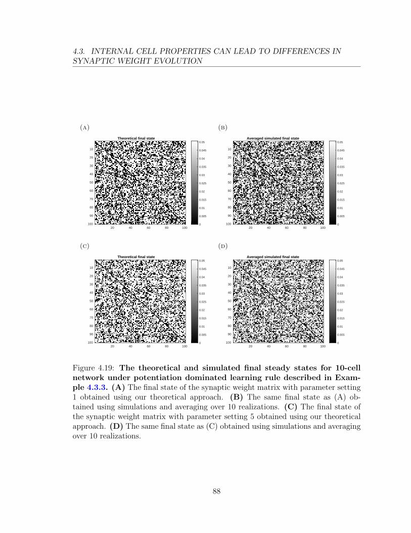
4.3. INTERNAL CELL PROPERTIES CAN LEAD TO DIFFERENCES INSYNAPTIC WEIGHT EVOLUTION
(a)
Theoretical final state
20 40 60 80 100
10
20
30
40
50
60
70
80
90
100 0
0.005
0.01
0.015
0.02
0.025
0.03
0.035
0.04
0.045
0.05
(b)
Averaged simulated final state
20 40 60 80 100
10
20
30
40
50
60
70
80
90
100 0
0.005
0.01
0.015
0.02
0.025
0.03
0.035
0.04
0.045
0.05
(c)
Theoretical final state
20 40 60 80 100
10
20
30
40
50
60
70
80
90
100 0
0.005
0.01
0.015
0.02
0.025
0.03
0.035
0.04
0.045
0.05
(d)
Averaged simulated final state
20 40 60 80 100
10
20
30
40
50
60
70
80
90
100 0
0.005
0.01
0.015
0.02
0.025
0.03
0.035
0.04
0.045
0.05
Figure 4.19: The theoretical and simulated final steady states for 10-cellnetwork under potentiation dominated learning rule described in Exam-ple 4.3.3. (A) The final state of the synaptic weight matrix with parameter setting1 obtained using our theoretical approach. (B) The same final state as (A) ob-tained using simulations and averaging over 10 realizations. (C) The final state ofthe synaptic weight matrix with parameter setting 5 obtained using our theoreticalapproach. (D) The same final state as (C) obtained using simulations and averagingover 10 realizations.
88
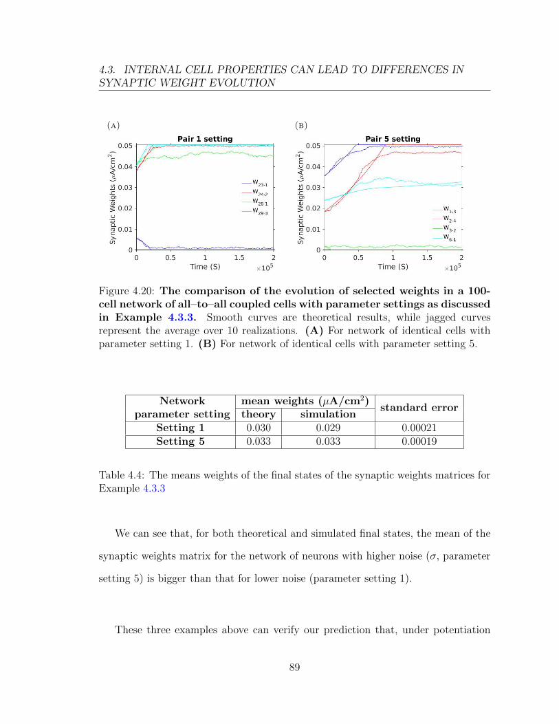
4.3. INTERNAL CELL PROPERTIES CAN LEAD TO DIFFERENCES INSYNAPTIC WEIGHT EVOLUTION
(a) (b)
Figure 4.20: The comparison of the evolution of selected weights in a 100-cell network of all–to–all coupled cells with parameter settings as discussedin Example 4.3.3. Smooth curves are theoretical results, while jagged curvesrepresent the average over 10 realizations. (A) For network of identical cells withparameter setting 1. (B) For network of identical cells with parameter setting 5.
Network mean weights (µA/cm2)standard error
parameter setting theory simulationSetting 1 0.030 0.029 0.00021Setting 5 0.033 0.033 0.00019
Table 4.4: The means weights of the final states of the synaptic weights matrices forExample 4.3.3
We can see that, for both theoretical and simulated final states, the mean of the
synaptic weights matrix for the network of neurons with higher noise (σ, parameter
setting 5) is bigger than that for lower noise (parameter setting 1).
These three examples above can verify our prediction that, under potentiation
89

4.4. PREDICT THE STEADY STATE UNDER BALANCED HEBBIAN STDPRULE
dominated Hebbian STDP rule, the synaptic weights of the networks of the neurons
with higher noise (σ, or lower drive µ) are more likely to strengthen than those of
the reversed case, even though all the neurons of all the different networks have the
same baseline firing rate.
4.4 Predict the steady state under balanced Heb-
bian STDP rule
Here we consider an ideal case: for some particular learning rules, we can predict
the steady state of a network after training just by giving its initial synaptic weight
matrix.
We apply balanced Hebbian STDP rule on 10-cell (with all-to-all connections)
networks of all the neurons with the same parameter setting in one network. The
initial synaptic weight matrices are the same for all networks and it is shown in
Figure 4.3A.
According to Eq.(2.6), we compute the matrices ofdWji
dtat the beginning of the
training (the first iteration for updating the weights under balanced Hebbian STDP
rule) for the networks of neurons with different parameter settings. We then define
a transformation of the matrices ofdWji
dtby replacing positive
dWji
dtvalue with 1 and
negativedWji
dtvalue with 0.
We find that, through the transformation we defined, the matrices ofdWji
dtare
90

4.4. PREDICT THE STEADY STATE UNDER BALANCED HEBBIAN STDPRULE
identical for all the 5 networks of neurons with the 5 parameter settings (µ-σ in Table
2.1, same setting for the neurons in the same network). We show it in Figure 4.21,
compared with the theoretical steady states of the synaptic weight matrices for the
5 networks after training (they are also identical).
(a)
matrix ofdWij
dtfor the beginning
2 4 6 8 10
1
2
3
4
5
6
7
8
9
100
0.1
0.2
0.3
0.4
0.5
0.6
0.7
0.8
0.9
1
(b)
Theoretical final state
2 4 6 8 10
1
2
3
4
5
6
7
8
9
100
0.1
0.2
0.3
0.4
0.5
Figure 4.21: The matrices ofdWji
dtafter transformation, and the theoretical
steady states of the weight matrices for all the 5 networks. (A) The ma-
trices ofdWji
dtafter transformation for all the 5 networks. They are identical. (B)
The theoretical steady states of weight matrices for the 5 networks. They are alsoidentical.
We can see that the above two matrices correspond with each other exactly. This
means that, under balanced Hebbian STDP rule, synaptic weight Wji will be po-
tentiated if its correspondingdWji
dtis positive at the beginning of the training, while
it will be depressed if the correspondingdWji
dtis negative. Thus, we can predict the
steady states of the networks under balanced Hebbian STDP rule just by computing
the matrix ofdWji
dtat the beginning of the training.
91

CHAPTER 5
Discussion and conclusions
In this dissertation, I examined the role of synaptic plasticity and the properties
of neuronal responses in shaping the architecture of recurrent networks. First, I
investigated synaptic weight dynamics in two-cell networks. Insights gained from
these networks allowed me to understand the evolution of the structure of larger
recurrent networks.
In Chapter 2, I introduced the the EIF neuron model which was used in the
remainder of the thesis. The EIF neuron has several properties that make it a more
faithful representation of an actual neuron than the Poisson model used in previous
studies. The EIF neuron model exhibits the same baseline firing rate but distinct
92
firing statistics at different parameter settings, unlike a Poisson neuron. Next, I
discussed the synaptic plasticity rule I used to model weight dynamics, the STDP
learning rule. Finally, I illustrated how to use linear response theory to approxi-
mated the cross-covariances for recurrent networks, a crucial step in the theoretical
approximation of synaptic weight evolution under STDP.
In Chapter 3, I used STDP, and the theoretical tools developed in Chapter 2
to both uni-and bi-directionally connected two-cell networks. I used networks with
fixed baseline firing rates for neurons in the same network, but different noise level
(σ value). With the same STDP learning rule, lower noise and higher common
input lead to faster weight evolution. Moreover, the shape of the cross-covariances
contributes more to the weight evolution in the case of f+τ+ = f−τ− in Eq.(3.3),
while the shape of the STDP governs weight evolution in other cases (f+τ+ 6= f−τ−).
In Chapter 4, I generalized the results for Chapter 3 to large networks (from
10-cell to 100-cell recurrent networks). if the same baseline firing rate for all neurons
in the network is the same, lower noise leads to faster weight evolution, as it did in
networks of two cells. Moreover, I studied the weight dynamics for large networks
with groups of neurons with different noise levels (µ − σ settings). With the same
baseline firing rate, the weights from neurons with higher noise (σ) to those with
lower noise are more likely to strengthen under a balanced Hebbian STDP rule.
However, with an Anti-Hebbian STDP rule, the opposite result holds: the weights
from neurons with lower noise to those with higher noise are more likely to strengthen.
I also considered asymmetric Hebbian STDP rules, in particular the potentiation
dominated case. In this case weights are potentiated in network of neurons with
93
higher noise. Last but not the least, for the symmetric Hebbian STDP rule, the
steady state of given network can be predicted from the the values of the derivatives
(positive or negative) of the synaptic weights at the beginning of weight evolution.
There are several interesting extensions of this work. For example, I have not
examined the effect of common input to the weight evolution of larger networks.
As shown in Chapter 2, a similar theoretical approach can be applied to this case.
Moreover, in this thesis, I just consider the EIF neuron model and Hebbian STDP
learning rules. However, many more detailed and physiologically realistic neuron
models and plasticity rule have been described in the literature. For example, the
Connor-Stevens neuron model [14] (which is considered to be more realistic than
EIF neuron model) and triplet STDP learning rule [26] are interesting examples
that could be studied using similar approaches. These neuron models and plasticity
rules could lead to different insights about the role of neuronal properties in shaping
network structure, but I leave them for future research.
94
Bibliography
[1] Morrison A, Aertsen A, and Diesmann M. Spike-timing-dependent plasticity inbalanced random networks. Neural Computation, 19:1437–1467, 2007.
[2] Cara B Allen, Tansu Celikel, and Daniel E Feldman. Long-term depressioninduced by sensory deprivation during cortical map plasticity in vivo. Natureneuroscience, 6(3):291–299, 2003.
[3] Babadi B and Abbott LF. Intrinsic stability of temporally shifted spike-timing dependent plasticity. PLoS Computational Biology, 6:e1000961.doi:10.1371/journal.pcbi.1000961., 2010.
[4] Babadi B and Abbott LF. Pairwise analysis can account for network struc-tures arising from spike-timing dependent plasticity. PLoS Comput Biol,9(2):e1002906. doi: 10.1371/journal.pcbi.1002906, 2013.
[5] Doiron B, Lindner B, Longtin A, Maler L, and Bastian J. Oscillatory activityin electrosensory neurons increases with the spatial correlation of the stochasticinput stimulus. Phys Rev Let, 93, 2004.
[6] Lindner B, Doiron B, and Longtin A. Theory of oscillatory firing induced byspatially correlated noise and delayed inhibitory feedback. Phys Rev E, 72, 2005.
[7] Laurent Badel, Sandrine Lefort, Thomas K Berger, Carl CH Petersen, WulframGerstner, and Magnus JE Richardson. Extracting non-linear integrate-and-fire
95

BIBLIOGRAPHY
models from experimental data using dynamic i–v curves. Biological cybernetics,99(4-5):361–370, 2008.
[8] Dorit Baras and Ron Meir. Reinforcement learning, spike-time-dependent plas-ticity, and the BCM rule. Neural Computation, 19(8):2245–2279, 2007.
[9] Olivier Bichler, Damien Querlioz, Simon J Thorpe, Jean-Philippe Bourgoin, andChristian Gamrat. Extraction of temporally correlated features from dynamicvision sensors with spike-timing-dependent plasticity. Neural Networks, 32:339–348, 2012.
[10] Allen C and Stevens C F. An evaluation of causes for unreliability of synaptictransmission. Proc. Natl. Acad. Sci., 91:10380–10383, 1994.
[11] Clopath C, Busing L, Vasilaki E, and Gerstner W. Connectivity reflects coding:a model of voltage-based STDP with homeostasis. Nature Neuroscience, 13:344–352, 2010.
[12] Gardiner C. Stochastic Methods: A Handbook for the Natural and Social Sci-ences. Springer, Berlin Heidelberg, 2009.
[13] Claudia Clopath and Wulfram Gerstner. Voltage and spike timing interact inSTDP–a unified model. Spike-timing dependent plasticity, page 294, 2010.
[14] JA Connor and CF Stevens. Prediction of repetitive firing behaviour fromvoltage clamp data on an isolated neurone soma. The Journal of Physiology,213(1):31, 1971.
[15] Lorente de No R. Transmission of impulses through cranial motor nuclei. JNeurophysiol, 2:402–64, 1939.
[16] Hebb DO. The organization of behavior: a neuropsychological theory. L. Erl-baum Associates, Mahwah, N.J., 1949.
[17] Izhikevich E, Gally J, and Edelman G. Spike-timing dynamics of neuronalgroups. Cerebral Cortex, 14:933–944, 2004.
[18] Lubenov E and Siapas A. Decoupling through synchrony in neuronal circuitswith propagation delays. Neuron, 58:118–131, 2008.
[19] Oja E. Simplified neuron model as a principal component analyzer. Journal ofMathematical Biology, 15:267–273, 1982.
96

BIBLIOGRAPHY
[20] Shimon Edelman and Nathan Intrator. Unsupervised statistical learning invision: computational principles, biological evidence. Miscellaneous Papers,Available from kybele. psych. cornell. edu, 23, 2004.
[21] Bienenstock EL, Cooper LN, and Munro PW. Theory for the development ofneuron selectivity: orientation specificity and binocular interaction in visualcortex. The Journal of Neuroscience, 2:32–48, 1982.
[22] Kandel ER and Tauc L. Mechanism of prolonged heterosynaptic facilitation.Nature, 202:145–147, 1964.
[23] Kandel ER and Tauc L. Heterosynaptic facilitation in neurones of the abdominalganglion of aplysia depilans. The Journal of Physiology, 181:1–27, 1965.
[24] Lugaro Ernesto. Modern Problems in Psychiatry. The University Press, Manch-ester, 1909.
[25] Nicolas Fourcaud-Trocme, David Hansel, Carl Van Vreeswijk, and NicolasBrunel. How spike generation mechanisms determine the neuronal responseto fluctuating inputs. The Journal of neuroscience, 23(37):11628–11640, 2003.
[26] Julijana Gjorgjieva, Claudia Clopath, Juliette Audet, and Jean-Pascal Pfister.A triplet spike-timing–dependent plasticity model generalizes the bienenstock–cooper–munro rule to higher-order spatiotemporal correlations. Proceedings ofthe National Academy of Sciences, 108(48):19383–19388, 2011.
[27] Bi GQ and Poo MM. Synaptic modifications in cultured hippocampal neuron-s: dependence on spike timing, synaptic strength, and postsynaptic cell type.Journal of Neuroscience, 18:10464–10472, 1998.
[28] Lynch GS, Dunwiddie T, and Gribkoff V. Heterosynaptic depression: a postsy-naptic correlate of long-term potentiation. Nature, 266:737–739, 1977.
[29] Markram H, Lubke J, Frotscher M, and Sakmann B. Regulation of synapticefficacy by coincidence of postsynaptic aps and epsps. Science, 275:213, 1997.
[30] Markram H, Gerstner W, and Sjostrom PJ. A history of spike-timing-dependentplasticity. Frontiers in Synaptic Neuroscience, 3:4, 2011.
[31] Abarbanel HDI, Gibb L, Huerta R, and Rabinovich MI. Biophysical model ofsynaptic plasticity dynamics. Biological Cybernetics, 89:214–226, 2003.
[32] Eugene M Izhikevich and Niraj S Desai. Relating stdp to bcm. Neural compu-tation, 15(7):1511–1523, 2003.
97
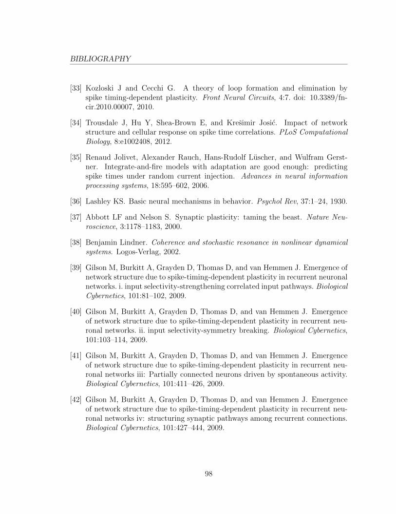
BIBLIOGRAPHY
[33] Kozloski J and Cecchi G. A theory of loop formation and elimination byspike timing-dependent plasticity. Front Neural Circuits, 4:7. doi: 10.3389/fn-cir.2010.00007, 2010.
[34] Trousdale J, Hu Y, Shea-Brown E, and Kresimir Josic. Impact of networkstructure and cellular response on spike time correlations. PLoS ComputationalBiology, 8:e1002408, 2012.
[35] Renaud Jolivet, Alexander Rauch, Hans-Rudolf Luscher, and Wulfram Gerst-ner. Integrate-and-fire models with adaptation are good enough: predictingspike times under random current injection. Advances in neural informationprocessing systems, 18:595–602, 2006.
[36] Lashley KS. Basic neural mechanisms in behavior. Psychol Rev, 37:1–24, 1930.
[37] Abbott LF and Nelson S. Synaptic plasticity: taming the beast. Nature Neu-roscience, 3:1178–1183, 2000.
[38] Benjamin Lindner. Coherence and stochastic resonance in nonlinear dynamicalsystems. Logos-Verlag, 2002.
[39] Gilson M, Burkitt A, Grayden D, Thomas D, and van Hemmen J. Emergence ofnetwork structure due to spike-timing-dependent plasticity in recurrent neuronalnetworks. i. input selectivity-strengthening correlated input pathways. BiologicalCybernetics, 101:81–102, 2009.
[40] Gilson M, Burkitt A, Grayden D, Thomas D, and van Hemmen J. Emergenceof network structure due to spike-timing-dependent plasticity in recurrent neu-ronal networks. ii. input selectivity-symmetry breaking. Biological Cybernetics,101:103–114, 2009.
[41] Gilson M, Burkitt A, Grayden D, Thomas D, and van Hemmen J. Emergenceof network structure due to spike-timing-dependent plasticity in recurrent neu-ronal networks iii: Partially connected neurons driven by spontaneous activity.Biological Cybernetics, 101:411–426, 2009.
[42] Gilson M, Burkitt A, Grayden D, Thomas D, and van Hemmen J. Emergenceof network structure due to spike-timing-dependent plasticity in recurrent neu-ronal networks iv: structuring synaptic pathways among recurrent connections.Biological Cybernetics, 101:427–444, 2009.
98

BIBLIOGRAPHY
[43] Gilson M, Burkitt A, Grayden D, Thomas D, and van Hemmen J. Emergenceof network structure due to spike-timing-dependent plasticity in recurrent neu-ronal networks v: self-organization schemes and weight dependence. BiologicalCybernetics, 103:1–22, 2010.
[44] Gilson M, Burkitt A, and van Hemmen J. STDP in recurrent neuronal networks.Frontiers in Computational Neuroscience, 4:23. doi: 10.3389/fncom.2010.00023,2010.
[45] Richardson M. Firing-rate response of linear and nonlinear integrate-and-fireneurons to modulated current-based and conductance-based synaptic drive.Physical Review E, 76:021919, 2007.
[46] Richardson M. Spike-train spectra and network response functions for non-linearintegrate-and-fire neurons. Biol Cybern, 99:381–392, 2008.
[47] Van Rossum M, Bi G, and Turrigiano G. Stable hebbian learning from spiketiming-dependent plasticity. Journal of neuroscience, 20:8812–21, 2000.
[48] Gabriel Koch Ocker, Ashok Litwin-Kumar, and Brent Doiron. Self-organizationof microcircuits in networks of spiking neurons with plastic synapses. PLoSComput Biol, 11(8):e1004458, 2015.
[49] Peter O’Connor, Daniel Neil, Shih-Chii Liu, Tobi Delbruck, and Michael Pfeiffer.Real-time classification and sensor fusion with a spiking deep belief network.Neuromorphic Engineering Systems and Applications, page 61, 2015.
[50] Srdjan Ostojic, Nicolas Brunel, and Vincent Hakim. How connectivity, back-ground activity, and synaptic properties shape the cross-correlation betweenspike trains. Journal of Neuroscience, 29(33):10234–10253, 2009.
[51] Gutig R, Aharonov R, Rotter S, and Sompolinsky H. Learning input correla-tions through nonlinear temporally asymmetric hebbian plasticity. Journal ofNeuroscience, 23:3697–3714, 2003.
[52] Kempter R, Gerstner W, and Van Hemmen JL. Hebbian learning and spikingneurons. Physical Review E, 59:4498, 1999.
[53] Kempter R, Gerstner W, and van Hemmen J. Intrinsic stabilization of outputrates by spike-based hebbian learning. Neural Computation, 13:2709–2741, 2001.
[54] Linsker R. From basic network principles to neural architecture: emergenceof spatial-opponent cells. Proceedings of the National Academy of Sciences,83:7508–7512, 1986.
99
BIBLIOGRAPHY
[55] Alexander Rauch, Giancarlo La Camera, Hans-Rudolf Luscher, Walter Senn,and Stefano Fusi. Neocortical pyramidal cells respond as integrate-and-fire neu-rons to in vivo–like input currents. Journal of neurophysiology, 90(3):1598–1612,2003.
[56] Douglas RM and Goddard GV. Long-term potentiation of the perforant path-granule cell synapse in the rat hippocampus. Brain Research, 86:205–215, 1975.
[57] Jonathan E Rubin, Richard C Gerkin, Guo-Qiang Bi, and Carson C Chow.Calcium time course as a signal for spike-timing–dependent plasticity. Journalof neurophysiology, 93(5):2600–2613, 2005.
[58] Song S, Miller K, and Abbott LF. Competitive hebbian learning through spike-timing-dependent synaptic plasticity. Nature Neuroscience, 3:919–26, 2000.
[59] Song S and Abbott LF. Cortical development and remapping through spiketiming-dependent plasticity. Neuron, 32:339–350, 2001.
[60] Michael N Shadlen and William T Newsome. The variable discharge of corticalneurons: implications for connectivity, computation, and information coding.Journal of neuroscience, 18(10):3870–3896, 1998.
[61] Yang SN, Tang YG, and Zucker RS. Selective induction of ltp and ltd bypostsynaptic [Ca2+]i elevation. Journal of Neurophysiology, 81:781–787, 1999.
[62] Charles F Stevens and A Zador. When is an integrate-and-fire neuron like apoisson neuron? Advances in neural information processing systems, pages103–109, 1996.
[63] Dunwiddie T and Lynch G. Long-term potentiation and depression of synapticresponses in the rat hippocampus: localization and frequency dependency. TheJournal of Physiology, 276:353–367, 1978.
[64] Lømo T. Frequency potentiation of excitatory synaptic activity in the dentatearea of the hippocampal formation. Acta Physiol Scand, 68, 1966.
[65] Simon J Thorpe. Spike-based image processing: can we reproduce biologicalvision in hardware? In European Conference on Computer Vision, pages 516–521. Springer, 2012.
[66] Sejnowski TJ. Storing covariance with nonlinearly interacting neurons. Journalof Mathematical Biology, 4:303–321, 1977.
100

BIBLIOGRAPHY
[67] Bliss TVP and Lømo T. Long-lasting potentiation of synaptic transmissionin the dentate area of the anaesthetized rabbit following stimulation of theperforant path. The Journal of Physiology, 232:331–356, 1973.
[68] Jacob V, Brasier DJ, Erchova I, Feldman D, and Shulz DE. Spike timing-dependent synaptic depression in the in vivo barrel cortex of the rat. TheJournal of neuroscience: the official journal of the Society for Neuroscience,27:1271–1284, 2007.
[69] Gerstner W, Kempter R, van Hemmen JL, and Wagner H. A neuronal learningrule for sub-millisecond temporal coding. Nature, 383:76–78, 1996.
[70] Gerstner W, Ritz R, and van Hemmen JL. Why spikes? hebbian learning andretrieval of time-resolved excitation patterns. Biological Cybernetics, 69:503–515, 1993.
[71] Levy WB and Steward O. Temporal contiguity requirements for long-termassociative potentiation/depression in the hippocampus. Neuroscience, 8:791–797, 1983.
[72] Li I Zhang, Huizhong W Tao, Christine E Holt, William A Harris, and Mu-ming Poo. A critical window for cooperation and competition among developingretinotectal synapses. Nature, 395(6697):37–44, 1998.
101