Copyright by Benjamin Jarrett Ebersole 2016
108
Copyright by Benjamin Jarrett Ebersole 2016
Transcript of Copyright by Benjamin Jarrett Ebersole 2016

Copyright
by
Benjamin Jarrett Ebersole
2016

The Thesis Committee for Benjamin Jarrett Ebersole
Certifies that this is the approved version of the following thesis:
Skid-Steer Kinematics for Dual-Arm Mobile Manipulator System with
Dynamic Center of Gravity
APPROVED BY
SUPERVISING COMMITTEE:
Sheldon Landsberger
Mitchell Pryor
Supervisor:
Co-Supervisor:
Skid-Steer Kinematics for Dual-Arm Mobile Manipulator System with
Dynamic Center of Gravity
by
Benjamin Jarrett Ebersole, B.S.
Thesis
Presented to the Faculty of the Graduate School of
The University of Texas at Austin
in Partial Fulfillment
of the Requirements
for the Degree of
Master of Science in Engineering
The University of Texas at Austin
December 2016

iv
Acknowledgements
I would like to thank my family, for their unconditional love and support over all
the years. I’d also like to thank my roommate and colleague Adam for being a patient and
wise sounding board for a never-ending stream of thoughts, questions, and word and
template formatting issues. And to my partner-in-crime on the VaultBot system, Andrew,
for helping to wrestle through all the amusing and frustrating quirks and oddities a robotic
system of that magnitude has to offer.
I am exceptionally grateful for my advisor Mitch Pryor’s support, guidance, and
technical advice throughout my time in the program. Sincere thanks also goes out to
Sheldon Landsberger for his fervent support of our program over the years. Thanks to Los
Alamos National Laboratories and the MET-2 division for their staunch financial and
organizational support for our program, and the excellent career opportunities they provide.
Finally, to all the members of the Nuclear and Applied Robotics Group for creating such a
fun and fascinating lab environment with a wealth of intellectual resources.

v
Abstract
Skid-Steer Kinematics for Dual-Arm Mobile Manipulator System with
Dynamic Center of Gravity
Benjamin Jarrett Ebersole, M.S.E
The University of Texas at Austin, 2016
Supervisor: Sheldon Landsberger
Co-Supervisor: Mitchell Pryor
Skid-steer mobile vehicles bridge an important operational gap in robotics between indoor-
only and outdoor-only platforms. Traditionally, skid-steer vehicles have been treated and
operated as differential-drive vehicles, which is an adequate approximation with a static
center of gravity (CG) coincident with the wheelbase center. With a dual-arm mobile
manipulator, such as the Nuclear and Applied Robotics Group's VaultBot platform, the
center of gravity's location is dynamic and the differential-drive model is no longer valid.
This can result in large errors between desired and actual trajectories over even short
periods of time. In this work, the degree to which the platform's behavior changes with a
dynamic CG and the intuition behind these effects are discussed. Several different
approaches leading to the development of a heuristic model built to improve performance,
and the evaluation results of said model, are also discussed.

vi
Table of Contents
Chapter 1: Introduction ............................................................................................1
1.1. Application ...............................................................................................1
1.2. Robotic System ........................................................................................2
1.3. Navigation Fundamentals ........................................................................4
1.3.1. Differential Steering.....................................................................4
1.3.2. Skid-Steering................................................................................6
1.4. Software Configuration ............................................................................7
1.4.1. ROS ..............................................................................................7
1.4.2. Default Controller ........................................................................9
1.5. Dynamic Center-of-Gravity ...................................................................11
1.6. Error Visualization/Verification ............................................................11
1.6.1. Setup ..........................................................................................11
1.6.2. Preliminary Results ....................................................................14
1.7. Motivation & Report Organization ........................................................14
Chapter 2: Literature Review .................................................................................16
2.1. Robotics in the Nuclear Domain ............................................................16
2.2. Mobile Manipulators ..............................................................................18
2.3. Skid Steer ...............................................................................................20
Chapter 3: Analytical Solution...............................................................................21
3.1. Full Kinematics ......................................................................................22
3.2. Force Analysis .......................................................................................25
3.3. Closed Form Solution ............................................................................28
3.4. Numerical Solvers ..................................................................................28
3.5. Summary ................................................................................................29
Chapter 4: Empirical Solutions ..............................................................................30
4.1. Neural Network ......................................................................................30
4.1.1. Vicon Motion Tracking..............................................................30
4.1.2. Implementation ..........................................................................32

vii
4.1.3. Results ........................................................................................32
4.2. Heuristic Model .....................................................................................33
4.2.1. Experimental Setup ....................................................................33
4.2.1.1. Hector SLAM.................................................................34
4.2.1.2. Center-of-Gravity Solver ...............................................35
4.2.1.3. Center-of-Rotation .........................................................37
4.2.2. Model Setup ...............................................................................38
4.2.3. Results ........................................................................................39
4.3. Conclusions & Implementation .............................................................55
Chapter 5: Demonstration ......................................................................................58
5.1. Setup ......................................................................................................58
5.2. Results ....................................................................................................60
Chapter 6: Conclusions and Future Work ..............................................................69
6.1. Research Summary ................................................................................69
6.2. Future Work ...........................................................................................71
6.3. Concluding Remarks ..............................................................................72
Appendix A: MATLAB Numerical Solver............................................................73
Appendix B: Result Trajectories ............................................................................75
References ..............................................................................................................93

viii
List of Tables
Table 4-1: Average Rotational Velocity Ratio to Cmd. Velocity ..........................43
Table 4-2: Center-of-Rotation x-position for given Center-of-Gravity .................45
Table 4-3: Center-of-Rotation y-position for given Center-of-Gravity .................47
Table 4-4: Multivariate Regression of CoR y-position for given CG, part 1 ........49
Table 4-5: Multivariate Regression of CoR y-position for given CG, part 2 ........50
Table 4-6: Multivariate Regression of CoR y-position for given CG, part 3 ........50
Table 4-7: Equation Coefficients for Linear Regression of Figure 4-10 data .......51
Table 5-1: Qualitative Evaluation of Skid-Steer Controller in 42 configurations .64
Table 5-2: Quantitative Evaluation of Skid-Steer Controller in 42 configurations66

ix
List of Figures
Figure 1-1: L – Rescue Robot “Quince” [5], M – Lancaster U. Decommissioning
Robot [8], R – Wall Decontamination Robot MANOLA [9] .............2
Figure 1-2: UT NRG’s “VaultBot” Mobile Manipulator ........................................3
Figure 1-3: Clearpath Husky ....................................................................................6
Figure 1-4: VaultBot ROS node layout example .....................................................8
Figure 1-5: Open Loop Trajectories with Varying CG [14]: (A) Legend mapping arm
configuration to color code. (B) “S-curve” trajectory. (C) “Arc”
trajectory. (D) In-place rotation. .......................................................13
Figure 3-1: Kinematic Analysis of a Skid-Steer Mobile Manipulator ...................22
Figure 4-1: VaultBot with Vicon Retroreflective Markers ....................................31
Figure 4-2: In-Place Rotation Position Tracking, COM-y position @ 0.02 ..........40
Figure 4-3: In-Place Rotation Smoothed Angular Velocities, COM-y position @ -0.03
...........................................................................................................42
Figure 4-4: Average Rotational Velocity Error Ratios vs. CG position ................44
Figure 4-5: Average Rotational Velocity Error Ratios vs. CG x-position .............44
Figure 4-6: Center-of-Rotation x-position vs. Center-of-Gravity position ............46
Figure 4-7: Center-of-Rotation x-position vs. Center-of-Gravity x-position ........46
Figure 4-8: Center-of-Rotation y-coordinate vs. Center-of-Gravity location ........48
Figure 4-9: Center-of-Rotation y-coordinate vs. Center-of-Gravity x-coordinate 48
Figure 4-10: Center-of-Rotation y-position vs. Center-of-Gravity y-position ......49
Figure 4-11: Multivariate Regression of CoR y-position for given CG; Results ..50
Figure 4-12: Slopes of Linear Regressions from Figure 4-10 vs. CG x-position ..52
Figure 4-13: Intercepts of Linear Regressions from Figure 4-10 vs. CG x-position52

x
Figure 4-14: Predicted vs. Measured CoR y-position with Full Model .................53
Figure 4-15: Predicted vs. Measured CoR y-position with Symmetric Model......54
Figure 5-1: Centers of Gravity for Controller Tests ..............................................58
Figure 5-2: Controller Odometry in Scurve Front Left Configuration ..................60
Figure 5-3: Controller Odometry in Arc #2 Back Right Configuration ................61
Figure 5-4: Controller Odometry in Rotate Ready Configuration .........................62
Figure 5-5: Controller Odometry in Arc #4 Ready Back Configuration ...............63
Figure 5-6: Controller Odometry in Arc #1 Ready Back Configuration ...............67
Figure 5-7: Controller Odometry in Arc #2 Front Right Configuration ................68
Figure 6-1: Open Loop Trajectories with Varying CG [14]: (A) Legend mapping arm
configuration to color code. (B) “S-curve” trajectory. (C) “Arc”
trajectory. (D) In-place rotation. .......................................................70
Figure B-1: Controller Odometry in Arc #1 Back Left Configuration ..................75
Figure B-2: Controller Odometry in Arc #1 Back Right Configuration ................75
Figure B-3: Controller Odometry in Arc #1 Front Left Configuration .................75
Figure B-4: Controller Odometry in Arc #1 Front Right Configuration ...............76
Figure B-5: Controller Odometry in Arc #1 Ready Configuration ........................76
Figure B-6: Controller Odometry in Arc #1 Ready Back Configuration ..............76
Figure B-7: Controller Odometry in Arc #1 Stow Back Configuration ................77
Figure B-8: Controller Odometry in Arc #2 Back Left Configuration ..................77
Figure B-9: Controller Odometry in Arc #2 Back Right Configuration ................77
Figure B-10: Controller Odometry in Arc #2 Front Left Configuration ...............78
Figure B-11: Controller Odometry in Arc #2 Front Right Configuration .............78
Figure B-12: Controller Odometry in Arc #2 Ready Configuration......................78
Figure B-13: Controller Odometry in Arc #2 Ready Back Configuration ............79

xi
Figure B-14: Controller Odometry in Arc #2 Stow Back Configuration ..............79
Figure B-15: Controller Odometry in Arc #3 Back Left Configuration ................80
Figure B-16: Controller Odometry in Arc #3 Back Right Configuration ..............80
Figure B-17: Controller Odometry in Arc #3 Front Left Configuration ...............81
Figure B-18: Controller Odometry in Arc #3 Front Right Configuration .............81
Figure B-19: Controller Odometry in Arc #3 Ready Configuration......................82
Figure B-20: Controller Odometry in Arc #3 Ready Back Configuration ............82
Figure B-21: Controller Odometry in Arc #3 Stow Back Configuration ..............83
Figure B-22: Controller Odometry in Arc #4 Back Left Configuration ................83
Figure B-23: Controller Odometry in Arc #4 Back Right Configuration ..............84
Figure B-24: Controller Odometry in Arc #4 Front Left Configuration ...............84
Figure B-25: Controller Odometry in Arc #4 Front Right Configuration .............84
Figure B-26: Controller Odometry in Arc #4 Ready Configuration......................85
Figure B-27: Controller Odometry in Arc #4 Ready Back Configuration ............85
Figure B-28: Controller Odometry in Arc #4 Stow Back Configuration ..............85
Figure B-29: Controller Odometry in Rotate Back Left Configuration ................86
Figure B-30: Controller Odometry in Rotate Back Right Configuration ..............86
Figure B-31: Controller Odometry in Rotate Front Left Configuration ................87
Figure B-32: Controller Odometry in Rotate Front Right Configuration ..............87
Figure B-33: Controller Odometry in Rotate Ready Configuration ......................88
Figure B-34: Controller Odometry in Rotate Ready Back Configuration .............88
Figure B-35: Controller Odometry in Rotate Stow Back Configuration ...............89
Figure B-36: Controller Odometry in S-curve Back Left Configuration ..............89
Figure B-37: Controller Odometry in S-curve Back Right Configuration ............90
Figure B-38: Controller Odometry in S-curve Front Left Configuration ..............90

xii
Figure B-39: Controller Odometry in S-curve Front Right Configuration ............91
Figure B-40: Controller Odometry in S-curve Ready Configuration ....................91
Figure B-41: Controller Odometry in S-curve Ready Back Configuration ...........92
Figure B-42: Controller Odometry in S-curve Stow Back Configuration .............92

1
Chapter 1: Introduction
1.1. APPLICATION
While the capabilities of artificial intelligence agents as portrayed in pop culture
and science fiction have long exceeded reality, the field of robotics may finally be catching
up to expectations. Previously dominated by specialized single task machines, such as
industrial workstations or dedicated vacuum cleaners, and carefully optimized laboratory
experiments and demonstrations, the field is now quickly growing to include increasingly
innovative and diverse applications in real-world scenarios. From headline-grabbing
efforts in self-driving passenger vehicles by major corporations such as Google and Tesla,
to lower profile yet still important advances in medical robotics, autonomous machines are
seeing increased development and usage across many different fields and disciplines.
One such area in which robots have seen increased demand for deployment is in
hazardous environments, particularly those found in the nuclear industry. The development
of autonomous devices to assist or even replace human workers in environments that would
be dangerous to those workers is a worthwhile endeavor. For example, recent events such
as the Fukushima Daiichi accident in 2011 [1] and the Waste Isolation Pilot Plant incident
in 2014 [2] have demonstrated the need for remote agents to enter and perform critical
tasks in high radioactivity zones, and many of these agents have been designed and
deployed, with varying levels of success [3][4]. Regardless of their design or primary tasks,
it is highly desirable that these agents be robust enough to successfully navigate uncertain,
cluttered, and sometimes dangerous terrain such that they can return safely upon
completion of the task. Some agents may also be required to complete high-effort tasks
such as opening doors or moving debris, whether as their primary mission or as a necessary
subtask to reach their primary mission. These agents must then be able to support and/or

2
manipulate significant payloads, and have sufficiently large operational workspaces for
successful manipulation.
1.2. ROBOTIC SYSTEM
Numerous mobile platforms and mobile manipulators have been developed for
nuclear and other hazardous environments [5][6][7]. These systems in recent years have
developed capabilities to move beyond simple teleoperation and execute tasks more
autonomously [8][9].
Figure 1-1: L – Rescue Robot “Quince” [5], M – Lancaster U. Decommissioning Robot
[8], R – Wall Decontamination Robot MANOLA [9]
One such system is the VaultBot, a mobile manipulator research platform in the
Nuclear and Applied Robotics Group at the University of Texas at Austin. The VaultBot
primarily consists of a 4-wheeled skid-steer Clearpath Husky mobile base platform with
two 6-DOF Universal Robotics “UR5” manipulators mounted above on a custom bulkhead.

3
Figure 1-2: UT NRG’s “VaultBot” Mobile Manipulator
The Husky base provides a wide, stable footprint which is sturdy enough to support
both arms, their controllers, and their payloads without any tipping, oscillation, or other
forms of movement in the base. Also, the 4 driven wheels provide additional traction and
redundant points of contact which help in navigation over loose soil and/or debris and
minimize chances of the robot getting stuck. These wheels are driven using a differential
steering system to minimize mechanical complexity and maximize durability and load
capability. However, unlike traditional differentially steered vehicles, the Husky’s
redundant, fixed wheels classify it as a “skid-steer” vehicle.
Much like tracked systems such as tanks or some construction equipment, wheeled
skid-steer vehicles rely on differing left and right side wheel velocity directions for
rotation. But unlike tracked systems, the smaller contact surface area for wheeled vehicles

4
typically produces less wear on themselves and the environment. These rotations depend
on lateral slip from the wheels, which introduces complex wheel-to-ground dynamic
interactions that are difficult to model. These then produce a mathematically complex,
nonlinear behavior for the vehicle as a whole, often depending on factors outside of the
vehicle itself such as terrain composition or slope. Due to these external factors, an exact
kinematic mapping of wheel input speeds to vehicle output motion cannot be precisely
determined. However, approximations can be made that approach the true behavior [10].
Because the control interfaces are at first quite similar (two motors, each controlling one
side of the robot), the differences between differentially steered and skid-steered vehicles
can at times be overlooked or over-simplified (see Clearpath’s controller implementation
in Section 1.4). In reality, however, the differences are significant and thus a major focus
of this work.
1.3. NAVIGATION FUNDAMENTALS
1.3.1. Differential Steering
An effective and commonly used design in mobile robotics, differential
steering consists of two independently driven, parallel wheels on the same fixed axis, with
another one or more passive wheels to stabilize the base. The design is effective because it
allows for a reasonable degree of maneuverability with almost zero slip; the robot can
rotate in place, travel forwards or backwards, or combine the two maneuvers for an arc-
like trajectory while the wheels maintain nearly pure rolling motion. The resulting
kinematic equations of motion for the vehicle translational and rotational velocities are:

5
𝑣𝑥 = 𝑟 (𝜔𝑙 + 𝜔𝑟
2 ) (1.1)
𝑣𝑦 = 0 (1.2)
�̇� = 𝑟 (𝜔𝑙 − 𝜔𝑟
𝐿) (1.3)
where ωl and ωr are the rotational velocities of the left and right wheels, r is the radius of
the wheels, and L is the distance between the wheels along the common axle, or the wheel
base. Note that vy is always 0; this reflects that at no instant in time may the vehicle move
directly sideways. However, differentially steered robots are frequently designed to be
close to if not fully rotationally symmetric, so that in-place turns are simple and of little
consequence from a collision perspective. Therefore, a differentially steered robot that
needs to make a lateral translation can deconstruct the move into three motions: a rotation
towards the goal, forwards motion to the goal location, and a final rotation to the desired
orientation. On smooth, planar, controlled surfaces, the differential steering design is
efficient, simple, and effective. On rougher terrain, however, having only 2 driven wheels
can quickly become a liability, leading to less stability, less traction, and a higher potential
for getting stuck.

6
1.3.2. Skid-Steering
Figure 1-3: Clearpath Husky
Skid-steer differential systems such as the Clearpath Husky (Figure 1-3) are similar
to standard differential systems in that they take 2 inputs, left and right wheel speed.
However, with 4 driven wheels and thus 4 points of contact, there is much more stability
for rough terrain. The Husky’s two left wheels are connected by a single drivetrain, and
likewise for the right side. At a glance, the kinematics are exactly the same: the husky may
move directly forwards or backwards by rotating the left and right wheels in the same
direction at the same speed, turn in place by rotating them in opposite directions at the same
speed, or any combination of the rotational and translational motions by varying the speeds
and directions. In reality, however, Equations 1.1-1.3 if implemented directly would
significantly overestimate the actual motion. Due to the redundant points of contact, there
is significant slip in any turning motion performed by the Husky, hence the term “skid-
steer”. Rotation of the vehicle about any point in space will cause at least two of the wheels
to have translation with components orthogonal to their plane of rotation. Preliminary
analysis has demonstrated that for any given in-place rotation, the resulting change in

7
orientation will be less than 50% of that which is predicted by the standard no-slip,
differential steering model.
1.4. SOFTWARE CONFIGURATION
1.4.1. ROS
The primary control structure of the system depends on ROS [11], an open-source
development framework that is becoming one of the ubiquitous software tools in robotics.
As it pertains to the VaultBot, a simple overview of ROS is as follows: A collection of
“nodes” act as drivers, to control and communicate with the various actuators, sensors, and
other hardware devices, or as processors, to react to and control the drivers as necessary.
These nodes primarily communicate by “publishing” data to “topics” that other nodes can
“subscribe” to for receiving data, or vice versa. As many as 21 of these nodes automatically
run on startup of the VaultBot, controlling and interfacing with systems such as the onboard
IMU, a joystick controller for teleoperation, and the SICK LIDAR LMS511 rangefinder,
and performing tasks such as diagnostic management and data filtration.
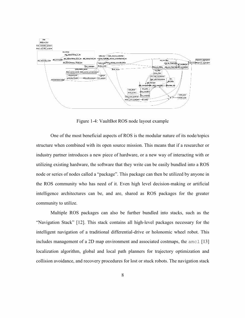
8
Figure 1-4: VaultBot ROS node layout example
One of the most beneficial aspects of ROS is the modular nature of its node/topics
structure when combined with its open source mission. This means that if a researcher or
industry partner introduces a new piece of hardware, or a new way of interacting with or
utilizing existing hardware, the software that they write can be easily bundled into a ROS
node or series of nodes called a “package”. This package can then be utilized by anyone in
the ROS community who has need of it. Even high level decision-making or artificial
intelligence architectures can be, and are, shared as ROS packages for the greater
community to utilize.
Multiple ROS packages can also be further bundled into stacks, such as the
“Navigation Stack” [12]. This stack contains all high-level packages necessary for the
intelligent navigation of a traditional differential-drive or holonomic wheel robot. This
includes management of a 2D map environment and associated costmaps, the amcl [13]
localization algorithm, global and local path planners for trajectory optimization and
collision avoidance, and recovery procedures for lost or stuck robots. The navigation stack

9
is utilized on the Husky platform, but as the VaultBot is not holonomic or truly differential-
drive there are significant performance issues. The localization package amcl, in
particular, diverges from the truth rapidly and is insufficient for safe autonomous operation
in its current state. One approach to solve this issue would be to rework amcl, or to attempt
to create or implement an entirely different localization algorithm, but this work chooses
to address the underlying faulty kinematic assumptions which cause the issue in the first
place.
1.4.2. Default Controller
For the Clearpath Husky mobile platform, the drivers which communicate with the
motors are in husky_node, which continuously subscribes to an assortment of topics.
One of these topics is cmd_vel, which accepts a translational velocity and a rotational
velocity vector. When data is published to the cmd_vel topic, husky_node pulls that
data, extracts the x velocity 𝑣𝑥 and z angular velocity θ, and feeds these into
diff_drive_controller to calculate the necessary right and left wheel velocities.
While not a node of its own, it is a generic controller used for differentially steered devices,
and handles both body velocity to wheel speed conversions and dead-reckoning odometry
calculations, using the following equations:
�̇�𝑙 =1
𝑤𝑟𝑟(�̇� −
𝑑𝑚𝑤𝑠�̇�
2) (1.4)
�̇�𝑟 =
1
𝑤𝑟𝑟(�̇� +
𝑑𝑚𝑤𝑠�̇�
2) (1.5)
�̇� =
𝑤𝑟𝑟(�̇�𝑙 + �̇�𝑟)
2 (1.6)
�̇� = 0 (1.7)
�̇� =
1
𝑑𝑚𝑤𝑠
[𝑤𝑟𝑟(�̇�𝑟 − �̇�𝑙)] (1.8)

10
where 𝑤𝑟 is the “wheel_radius_multiplier”; r is the wheel radius; 𝑤𝑠 is the
“wheel_separation_multiplier”; �̇�, �̇�, and �̇� are the vehicle linear and angular
velocities; 𝑑𝑚 is the wheel base of the vehicle; and �̇�𝑙 and �̇�𝑟 are the left and right wheel
speeds. With the exception of the multiplier terms, these are the same basic differential
steering equations as Equations 1.1-1.3. The multipliers are typically set to 1.0 and are used
as slight tuning parameters, but in the case of the VaultBot are slightly different. Due to
the unique power requirements of carrying two industrial manipulators, their controllers,
and their payloads, the Husky base was outfitted with a unique gear train. This resulted in
a modification of the motor to wheel relationship, and is most easily accounted for in 𝑤𝑟.
Clearpath recommended setting this parameter to a general value of 0.5, but
experimentation (comparison of raw encoder output to observation of a set number of
wheel rotations) revealed a more accurate value of 0.527. This is a constant parameter, so
future references to control equations will assume this value to be folded into 𝑟 itself for
simplicity. The second multiplier, 𝑤𝑠, is the primary heuristic used to approximately
account for the slip inherent to the Husky’s skid steer configuration. Set to a value of 1.875,
the value appears to be a fair correction under default operating conditions. However, as
will be discussed in future sections, the dynamic nature of the robot’s manipulators results
in operating conditions that are often far from the default.
Once the desired wheel speeds have been calculated, husky_node then uses a
speed control feedback loop, in conjunction with wheel encoders, to set and maintain the
wheels at those speeds until a new value is given.

11
1.5. DYNAMIC CENTER-OF-GRAVITY
In addition to the standard challenges offered by a skid-steer vehicle, observations
of in-place rotations during testing operations have indicated that the VaultBot tends to
rotate about its center-of-gravity (CG). This is significant because the VaultBot has the
challenging additional characteristic of a highly variable CG due to its manipulators and
potentially varying (and substantial) payloads. Therefore, at any given time the mobile base
could behave differently depending on the positions of the mobile manipulators and/or their
payloads.
As mentioned previously, the default controller for the Husky platform is a
differential-steer controller with a heuristic constant multiplier to account for the slip.
While this is a roughly valid approximation for the base’s behavior in the VaultBot’s
default configuration (with the arms stowed close to the base), it is far from ideal and
diverges from the truth rapidly when in non-default configurations.
1.6. ERROR VISUALIZATION/VERIFICATION
In order to evaluate the existence and severity of potential errors introduced by an
odometry model which does not account for a dynamic CG, an experiment was setup to
compare various open-loop maneuvers with changing arm configurations.
1.6.1. Setup
In order to test the effects of a changing CG, the VaultBot was given open-loop
commands for three separate behaviors while in three different arm configurations,
resulting in 9 trajectories. A camera was positioned on a tripod on a balcony overlooking
the test area, and video was taken of each experiment. Note that for each group of

12
configurations for a given behavior, the robot’s base started at the same position and
orientation.
For these preliminary experiments, all arm positions were longitudinally
symmetric. Therefore, the CG was assumed to be located on the x-axis for all tests. As
shown in Figure 1-5a, the first arm configuration was the standard “back stow” position,
with the arms tucked closely into the body and the elbows towards the rear of the vehicle.
Due to the mounting configuration of the arms, this results in the CG being closest to the
center of the wheel base of the 3 configurations. The second configuration was “front
stow”, again with the arms tucked closely to the body but with the elbows in front of the
vehicle, thus moving the CG forwards. The third configuration was “ready”, with the arms
deployed forwards as if ready to manipulate an object in front of the vehicle, moving the
CG even farther along the x-axis.
The first open loop behavior was the “Arc” behavior, with constant forward and
rotational velocities:
𝑣𝑥 = 0.5 𝑚/𝑠
�̇� = −0.2 𝑟𝑎𝑑/𝑠} 𝑓𝑜𝑟 0 < 𝑡 < 6.0𝑠 (1.9)
The second behavior was the “S-curve” trajectory, with a constant forward velocity
and a sinusoidal rotational velocity:
𝑣𝑥 = 0.8 𝑚/𝑠
�̇� = −0.6 ∗ sin (2𝜋𝑡
9.0) 𝑟𝑎𝑑/𝑠
} 𝑓𝑜𝑟 0 < 𝑡 < 9.0𝑠 (1.10)
The final behavior was a simple in-place rotation:

13
𝑣𝑥 = 0 𝑚/𝑠
�̇� = −0.5 𝑟𝑎𝑑/𝑠} 𝑓𝑜𝑟 0 < 𝑡 < 3.0𝑠 (1.11)
Finally, in order to verify the repeatability of the tests, the “back stow”
configuration and “S-curve” trajectory combination was repeated 3 times. Under these
controlled conditions with the same arm configurations and open loop commands, the
difference in final positions was negligible.
Figure 1-5: Open Loop Trajectories with Varying CG [14]: (A) Legend mapping arm
configuration to color code. (B) “S-curve” trajectory. (C) “Arc” trajectory.
(D) In-place rotation.
14
1.6.2. Preliminary Results
Once the tests were completed, the starting and ending position shots for each test
were extracted from the video. They were then digitally overlaid on top of each other, for
comparison in Figure 1-5b - Figure 1-5d. For clearest comparison, the 3 arm configurations
were given a color code, and then a rectangular portion of the VaultBot’s mounting bracket
was traced in each configuration’s respective color. The starting position was represented
by a white rectangle. For the “Arc” and “S-curve” behaviors, rough approximations of the
trajectory were sketched as well. As can be seen from the photos, a clear difference can be
seen when the center-of-gravity changes. Over a relatively short distance in the “S-curve”
behavior, the VaultBot in the “ready” configuration ends up at a significantly different
location from when in the “back stow” arrangement. In all 3 behaviors, the CG’s distance
forwards along the x-axis appears to correspond to more rotation for a given command;
this is particularly evident with the in-place rotation behavior.
The primary purpose of these experiments was to experimentally validate the
hypothesis that the error was significant. In the three configurations, the CG was estimated
to move by up to 0.25 meters which was determined from video analysis of the in-place
rotation behaviors, which also showed a rotation difference of as much as 55 degrees. And
in the translational trajectories, the difference in the target locations was estimated to be up
to 0.85 meters. This verifies that the error is significant, and validates the efforts to address
it.
1.7. MOTIVATION & REPORT ORGANIZATION
For open-loop navigation procedures such as teleoperation, the benefits of
improving the kinematic model are readily apparent; a robot which behaves as expected

15
improves user experience and performance. Autonomous behavior, however, typically
relies on closed loop navigation processes which, if utilizing sufficiently powerful sensors
and computational power, can often “wash over” modeling errors. Nevertheless, the
probabilistic closed loop models widely used in robotics today still utilize an open-loop
model of the system for the “prediction” step, and a significantly inaccurate model adds
unnecessary computational effort to the system and increases the likelihood of divergent
behavior. Therefore, efforts to improve the underlying kinematic model should bear fruit
in multiple capacities.
The objectives of this work are as follows: Commonly available motion planners
and previous skid-steer kinematic modeling efforts will be reviewed in Chapter Two to see
if they address the issue of a variable CG, and then their effectiveness will be evaluated.
Then a review of various attempts made at deriving an analytic solution to a more accurate
kinematic model will be covered in Chapter Three. Next, a discussion of attempted empiric
solutions, including the final heuristic solution and lessons learned from its derivation, will
be presented in Chapter Four. Chapter Five will contain a comparison of the solution
against the default controller and an evaluation of the success of the model. Finally,
concluding thoughts and a discussion of future work will comprise Chapter Six.

16
Chapter 2: Literature Review
2.1. ROBOTICS IN THE NUCLEAR DOMAIN
The need for robotic solutions in the nuclear domain is not a recently realized
concept. Raymond C. Goertz was one of the earliest adopters, utilizing telerobotics at
Argonne National Laboratory in 1949 to handle radioactive material [15]. In 1985, Moore
[16] published an extensive review of robotics in the nuclear power industry, discussing
robots by companies such as Westinghouse involved in inspection and maintenance
processes, as well as DOE-supplied robots to assist with cleanup of the Three Mile Island
incident. Briones et al. [17] in 1994 introduced prototypes for a wall-climbing robot
designed for inspection in boiling water reactor (BWR) plants, using suction cups and
flexible components to navigate up and across vertical surfaces. Ishikawa and Suzuki [18]
proposed a collaborative, semi-autonomous approach to controlling a rudimentary mobile
robot for use in nuclear power plants in 1997. Finally, Iwano et al. [19] in 2004 presented
a conceptual design of swarm rescue robots, to safely recover injured or incapacitated
humans from the scene of a nuclear plant accident such as the criticality accident at Japan’s
Tokai Factory of Nuclear Fuel Conversion Plant in 1999. Nevertheless, the pace at which
these technologies were developed and introduced pales in comparison to the innovations
spurred by recent events.
Modern nuclear incidents, such as the crisis at the Fukushima Daiichi Nuclear
Power Station in March 2011 and the spill at the Waste Isolation Pilot Plant in New Mexico
in February 2014, spurred many robotic companies and researchers around the world into
action. For example, Nagatani et al. [5] represented a collaborative effort amongst
researchers from 3 Japanese universities to retrofit a mobile rescue robot named Quince
for survey, exploration, and measurement missions in the damaged nuclear complex. Later,

17
Nagatani et al. published an update [1] on their successes and failures, and discussed plans
for continued operation with improved iterations of the Quince robot. Other efforts arose
not in direct response to the events at Fukushima, but as a result of the political
repercussions. Notheis et al. [9] presented designs for a decommissioning robot system
named MANOLA in response to Germany’s mandate to shut down all nuclear power plants
by 2022, which in turn was in direct response to the Fukushima incident. A complex design,
MANOLA is a wall-climbing robot equipped with tools for laser ablation of surfaces, and
with an accompanying mobile transport system to deliver MANOLA to the correct walls.
Other decommissioning efforts include work by Besset and Taylor [8] of Lancaster
University in the UK; RICA, a mobile sampling robot by Ducros et al. [20] of the CEA
(French Atomic Energy Commission); and AVEXIS, a series of underwater robotic
vehicles by Griffiths et al. [4] for use in storage ponds as part of the decommissioning of
the Sellafield nuclear facilities in Cumbria, U.K.
One of the more exotic applications is presented by Jiang et al. [21] in response to
the WIPP spill. In order to inspect and swab the surface of the exhaust shaft, which was
subject to radioactive smoke due to the incident, Jiang et al. propose a semi-autonomous
flying drone: the Dextrous Hexrotor. In the paper they discuss initial designs, solution
prototypes, and testing inside a grain solo.
Even without the motivation of a specific event, development for robotics
applications in hazardous environments continues. Huang et al. [7] propose a mobile
robotic solution for CBRN sampling; that is, flexible for applications in Chemical,
Biological, Radiological, and Nuclear incident response. RIANA is a mobile robot solution
presented by Kanaan et al. [22] of the French nuclear energy company AREVA, “dedicated

18
for investigations and assessments of nuclear Areas”, while Li et al. [6] propose a mobile
robot for “environment monitoring”.
While many significant efforts have clearly been made in nuclear robotics, a
majority of these efforts have been single-track; that is, they were specially engineered and
utilized for specific tasks and end-users. While this specialization is a valid approach in
some aspects, it limits the potential for shared knowledge and increases the occurrence of
separate research teams repeating the same mistakes. A university focused research effort,
such as the Nuclear and Applied Robotics Group at UT Austin, allows for broader efforts
utilizing open-source software and the academic community to design systems accessible
to multiple applications and user bases.
2.2. MOBILE MANIPULATORS
While plenty of robotic solutions consist solely of one or several fixed
manipulators, or of a mobile sensing robot with cameras and other sensors but no additional
actuators, much greater mission flexibility can be achieved with the marriage of these two
concepts: a mobile manipulator. While it can also be equipped with sensing and
environment monitoring devices, the primary design intent of a mobile manipulator is
typically to interact with the environment in some way, whether it be retrieving material,
opening doors, or even rescuing people in harm’s way. Some previously discussed efforts
which fit into the mobile manipulator classification include: Quince by Nagatani et al. [1],
[5]; the unnamed robotic solutions proposed by Besset and Taylor [8] and Huang et al. [7],
RIANA by Kanaan et al. [22], and RICA by Ducros et al. [20]. Unfortunately, there is little
discussion within these papers on the navigation or operation of the mobile base. Also,
with the exception of RIANA, all of these solutions have tracked wheel systems. RIANA

19
on the other hand is a 4-wheeled skid steer system with a 3 DOF manipulator arm, and is
perhaps the closest modern solution in the nuclear domain to the VaultBot. Navigation is
only briefly discussed, however, and “the precision of the navigation… depends on the
environment and the used sensors”, indicating complete reliance on closed-loop sensing.
Outside of the nuclear domain, mobile manipulators take on a much broader
spectrum of designs and approaches. Trulls et al. [23] discuss the navigation aspects of
Segway-based service robots in urban scenarios, while Stentz et al. [24] introduce CHIMP,
a highly complex, humanoid system developed by Carnegie Mellon University for the
DARPA Robotics Challenge. CHIMP is designed to drive on two tracked legs, or lower
onto its arms as well for 4-tracked mobility. Even non-wheeled solutions are being
developed, such as RoboSimian by Hebert et al. [25], “a statically stable quadrupedal
robot” which uses multi-jointed limbs as traversal implements as well as manipulation
tools. Ben-Tzvi [26] of George Washington University presents a small, geometrically
symmetrical tracked platform with a closely integrated 2-DOF arm that assists in mobility
when not performing manipulation tasks, which is claimed to result in a much higher
payload capacity than is typical for mobile manipulators.
While most of these works concern themselves with the design and implementation
of their novel robot concept as a whole, some works take a more theoretical approach and
more closely analyze the relationship between a robot’s mobility given the presence of a
manipulator, or conversely manipulation capabilities and procedures given the additional
platform mobility. Addressing the former, He [27] proposes a “tip-over avoidance
algorithm” for mobile manipulators, moving the manipulator as necessary to manage
multiple dynamic scenarios such as non-level surfaces and high turning speeds. Ide et al.
20
[28] present an example of the latter, using model predictive control to unify control and
trajectory planning of a manipulator and a differentially steered mobile base.
The most relevant work to this thesis is likely that presented by Liu and Liu [29] of
Ryerson University in Toronto. In their work, Liu and Liu create a thorough kinetic and
kinematic model of a proposed mobile manipulator with a tracked base and a single
manipulator arm. Importantly, this model makes the simplifying assumption that the
tracked system behaves as a six-wheeled skid-steer base, and the kinetic model takes into
account the forces induced by the manipulator position and motion, as well as any external
forces on the end-effector (such as payloads). However, their model is solved and utilized
in simulation, rather than real time. A closer analysis of their approach and lessons learned
are discussed in Chapter 3.
2.3. SKID STEER
The specific configuration of the VaultBot’s mobile base, wheeled skid-steer, has
also been the subject of plentiful research. Several groups have investigated better closed-
loop control of skid-steer vehicles, such as Caracciolo et al.[30], the extending work of
Kowzlowski et al. [31], and Pentzer et al. [32] of Pennsylvania State University. These
implementations, while thorough and effective, all depend on a measurement input of the
robot’s state independent of odometry during operation, typically GPS. Mandow et al. [33]
discuss methods for experimental development of a better kinematic model, which is then
utilized real-time for improved performance. However, although they discuss the potential
effects of different center-of-gravity locations, it is not implemented into the model and the
CG is assumed to be constant.

21
Chapter 3: Analytical Solution
Based on dynamic models found in the literature and related efforts to solve this or
similar problems, several approaches were attempted in finding a solution to the presented
problem. These included:
A closed form analytical model
A numerical solution to the analytical model
Neural network training
A heuristic model
This chapter discusses approaches using the comprehensive full kinematic and
dynamic models in order to find an analytical solution. If possible, it would then be possible
to much more accurately control and track the motion of the robot as desired based on
wheel speeds and arm configurations. This approach proved untenable due to significant
complexities introduced by the nonlinearities defining the tire/ground interactions.
However, the approach is documented here to assist with any future efforts that consider
this approach. Furthermore, it may be possible to simplify or validate the presented models
in future efforts by utilizing the following empirical results. For the eventual solution
employed in this paper, see Section 5.2.

22
3.1. FULL KINEMATICS
Figure 3-1: Kinematic Analysis of a Skid-Steer Mobile Manipulator
Based on the work of Liu and Liu [29], an attempt was made to model and solve
the full kinematic model of the mobile manipulator, including the nonlinear slip
interactions at the four wheels. Though Liu and Liu worked with a tracked vehicle, their
treatment of the vehicle as a six-wheeled skid-steer platform allows for a natural extension
to the VaultBot’s four-wheeled setup. Also, the presence of an additional manipulator arm
on the VaultBot should only add tedium to the calculations, but not additional complexity,
particularly if the two are represented by a single composite center-of-gravity. The primary

23
coordinate frames are as follows: 𝑂𝑚 − 𝑋𝑚𝑌𝑚𝑍𝑚 is a fixed local frame, where the
coordinate plane 𝑋𝑚𝑂𝑚𝑌𝑚 is parallel to the ground and passes through all wheel axes, so
it has a positive z offset equal to the wheel radius. 𝑂𝑚𝑋𝑚 points directly forwards to the
front of the vehicle, and therefore the positive direction of 𝑂𝑚𝑌𝑚 is to the left. The location
of the vehicle’s CG is represented as the dynamic coordinate frame 𝑂𝐺 − 𝑋𝐺𝑌𝐺𝑍𝐺 , which
maintains the same orientation as frame 𝑂𝑚 − 𝑋𝑚𝑌𝑚𝑍𝑚 but is subject to dynamic
translations, represented by 𝑥𝐺𝑚, 𝑦𝐺
𝑚, 𝑧𝐺𝑚, and their time derivatives. Liu and Liu also present
an inertial base frame 𝑂𝐵 − 𝑋𝐵𝑌𝐵𝑍𝐵, resulting in the following dynamic equations:
�̇�𝑚 =
[𝑟(�̇�𝑙 + �̇�𝑟) + (�̇�𝑙𝑥 + �̇�𝑟𝑥)]𝑐𝑜𝑠𝜙𝑚
2
+𝑑0[𝑟(�̇�𝑟 − �̇�𝑙) + (�̇�𝑟𝑥 − �̇�𝑙𝑥)]𝑠𝑖𝑛𝜙𝑚
𝑑𝑚
(3.1)
�̇�𝑚 =
[𝑟(�̇�𝑙 + �̇�𝑟) + (�̇�𝑙𝑥 + �̇�𝑟𝑥)]𝑠𝑖𝑛𝜙𝑚
2
−𝑑0[𝑟(�̇�𝑟 − �̇�𝑙) + (�̇�𝑟𝑥 − �̇�𝑙𝑥)]𝑐𝑜𝑠𝜙𝑚
𝑑𝑚
(3.2)
�̇�𝑚 =
1
𝑑𝑚
[𝑟(�̇�𝑟 − �̇�𝑙) + (�̇�𝑟𝑥 − �̇�𝑙𝑥)] (3.3)
where �̇�𝑚, �̇�𝑚, 𝜙𝑚 represent the linear velocities and heading of the mobile platform
relative to the base frame, 𝑟 is the wheel radius, �̇�𝑙 , �̇�𝑟 are the left and right wheel speeds,
�̇�𝑙𝑥, �̇�𝑟𝑥 are the longitudinal slip values of the left and right wheel sets, 𝑑𝑚 is the width of
the vehicle track, and 𝑑0 is the offset along 𝑂𝑚𝑋𝑚 of the instantaneous Center-of-Rotation
(CoR). However, as this effort is only concerned with the local movement and velocities
of the VaultBot, frames 𝑂𝑚 − 𝑋𝑚𝑌𝑚𝑍𝑚 and 𝑂𝐵 − 𝑋𝐵𝑌𝐵𝑍𝐵 are assumed to be always
coincident at any given time, with the exception of the z offset which is a constant.
Therefore:
24
𝑥𝑚 = 𝑦𝑚 = 𝜙𝑚 = 0, 𝑧𝑚 = 𝑟
which allows the ‘m’ subscript to be dropped and results in the simplified equations:
�̇� =[𝑟(�̇�𝑙 + �̇�𝑟) + (�̇�𝑙𝑥 + �̇�𝑟𝑥)]
2 (3.4)
�̇� = −𝑑0[𝑟(�̇�𝑟 − �̇�𝑙) + (�̇�𝑟𝑥 − �̇�𝑙𝑥)]
𝑑𝑚= −𝑑0�̇� (3.5)
�̇� =1
𝑑𝑚
[𝑟(�̇�𝑟 − �̇�𝑙) + (�̇�𝑟𝑥 − �̇�𝑙𝑥)] (3.6)
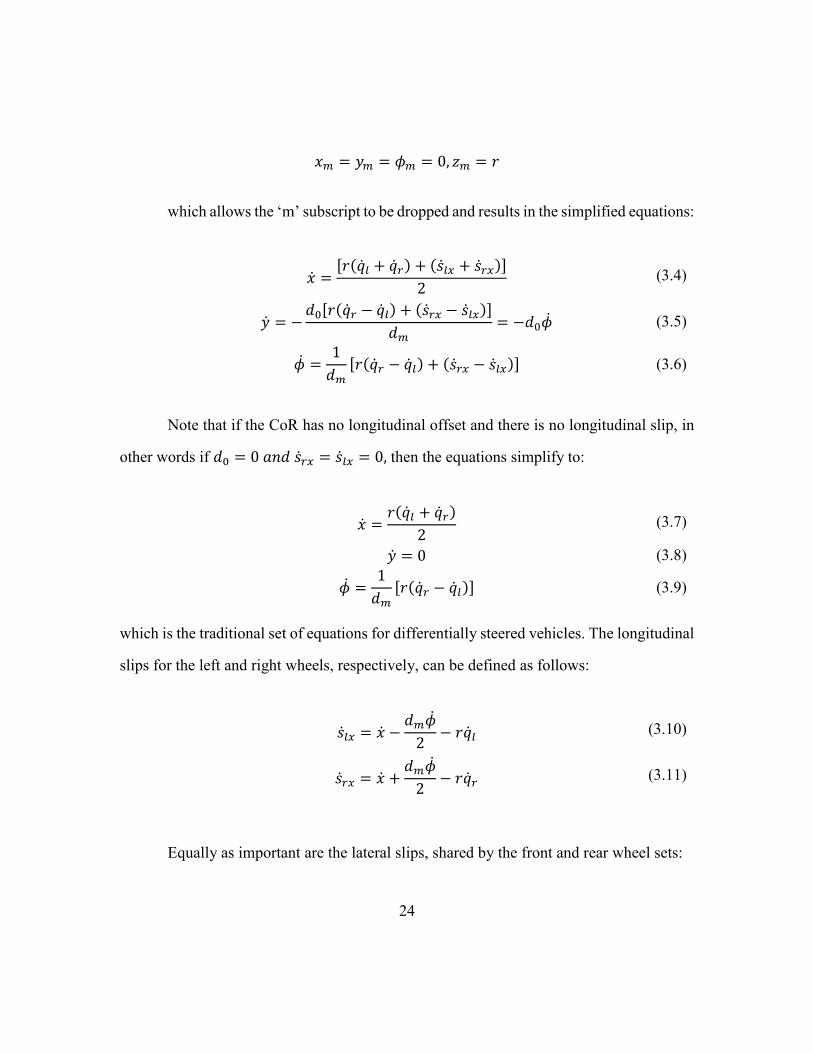
Note that if the CoR has no longitudinal offset and there is no longitudinal slip, in
other words if 𝑑0 = 0 𝑎𝑛𝑑 �̇�𝑟𝑥 = �̇�𝑙𝑥 = 0, then the equations simplify to:
�̇� =𝑟(�̇�𝑙 + �̇�𝑟)
2 (3.7)
�̇� = 0 (3.8)
�̇� =1
𝑑𝑚
[𝑟(�̇�𝑟 − �̇�𝑙)] (3.9)
which is the traditional set of equations for differentially steered vehicles. The longitudinal
slips for the left and right wheels, respectively, can be defined as follows:
�̇�𝑙𝑥 = �̇� −𝑑𝑚�̇�
2− 𝑟�̇�𝑙 (3.10)
�̇�𝑟𝑥 = �̇� +𝑑𝑚�̇�
2− 𝑟�̇�𝑟 (3.11)
Equally as important are the lateral slips, shared by the front and rear wheel sets:

25
�̇�𝑓𝑦 = �̇� + 𝑙𝑓�̇� (3.12)
�̇�𝑏𝑦 = �̇� + 𝑙𝑏�̇� (3.13)
𝑙𝑓 = −𝑙𝑏 =𝑊𝑏
2 (3.14)
where 𝑊𝑏 is the VaultBot wheel base. These slips occur at the four wheel contact points:
𝑃𝑓𝑙, 𝑃𝑓𝑟 , 𝑃𝑏𝑙, 𝑃𝑏𝑟 where the subscripts ‘fl’, ‘fr’, ‘bl’, and ‘br’ correspond to ‘front left’, ‘front
right’, ‘back left’, and ‘back right’ respectively.
3.2. FORCE ANALYSIS
The friction and resistance forces at the wheels then are modeled the same as in the
work of Liu and Liu:
𝐹⋆◊
𝑥 = −𝜇𝑥𝑁⋆◊ [1 − exp (−𝐾|�̇�◊𝑥|
max(|�̇�◊𝑥 + 𝑟�̇�◊|, |𝑟�̇�◊|))]
�̇�◊𝑥
√�̇�◊𝑥2 + �̇�⋆𝑦
2
(3.15)
𝐹⋆◊
𝑦= −𝜇𝑦𝑁⋆◊[1 − exp(−𝐾)]
�̇�⋆𝑦
√�̇�◊𝑥2 + �̇�⋆𝑦
2
(3.16)
𝑅⋆◊ = 𝑓𝑟𝑁⋆◊ (3.17)
where ‘⋆’ represents ‘f’ or ‘b’; ‘◊’ represents ‘l’ or ‘r’; 𝜇𝑥, 𝜇𝑦 are the friction coefficients
between the tire material and the ground, 𝐾 is a constant “determined by pull slip test”, 𝑁
represents the normal force at the contact point, and 𝑓𝑟 is the coefficient of motion
resistance, also experimentally determined. The inertial accelerations of the CG are also
the same, with the addition of the 𝜙𝑚 = 0 simplification:
�̈�𝐺𝐵 = �̈�𝑚
𝐵 + �̈�𝐺𝑚 − 𝑦𝐺
𝑚�̈� − 2�̇�𝐺𝑚�̇� − 𝑥𝐺
𝑚�̇�2 (3.18)
�̈�𝐺𝐵 = �̈�𝑚
𝐵 + �̈�𝐺𝑚 + 𝑥𝐺
𝑚�̈� + 2�̇�𝐺𝑚�̇� − 𝑦𝐺
𝑚�̇�2 (3.19)
26
�̈�𝐺𝐵 = �̈�𝐺
𝑚 (3.20)
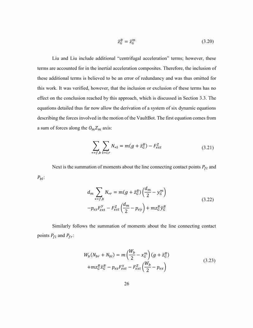
Liu and Liu include additional “centrifugal acceleration” terms; however, these
terms are accounted for in the inertial acceleration composites. Therefore, the inclusion of
these additional terms is believed to be an error of redundancy and was thus omitted for
this work. It was verified, however, that the inclusion or exclusion of these terms has no
effect on the conclusion reached by this approach, which is discussed in Section 3.3. The
equations detailed thus far now allow the derivation of a system of six dynamic equations
describing the forces involved in the motion of the VaultBot. The first equation comes from
a sum of forces along the 𝑂𝑚𝑍𝑚 axis:
∑ ∑ 𝑁⋆◊
◊=𝑙,𝑟⋆=𝑓,𝑏
= 𝑚(𝑔 + �̈�𝐺𝐵) − 𝐹𝑒𝑥𝑡
𝑍 (3.21)
Next is the summation of moments about the line connecting contact points 𝑃𝑓𝑙 and
𝑃𝑏𝑙:
𝑑𝑚 ∑ 𝑁⋆𝑟
⋆=𝑓,𝑏
= 𝑚(𝑔 + �̈�𝐺𝐵) (
𝑑𝑚
2− 𝑦𝐺
𝑚)
−𝑝𝑒𝑧𝐹𝑒𝑥𝑡𝑦
− 𝐹𝑒𝑥𝑡𝑍 (
𝑑𝑚
2− 𝑝𝑒𝑦) + 𝑚𝑧𝐺
𝐵�̈�𝐺𝐵
(3.22)
Similarly follows the summation of moments about the line connecting contact
points 𝑃𝑓𝑙 and 𝑃𝑓𝑟:
𝑊𝑏(𝑁𝑏𝑟 + 𝑁𝑏𝑙) = 𝑚 (
𝑊𝑏
2− 𝑥𝐺
𝑚) (𝑔 + �̈�𝐺𝐵)
+𝑚𝑧𝐺𝐵�̈�𝐺
𝐵 − 𝑝𝑒𝑧𝐹𝑒𝑥𝑡𝑥 − 𝐹𝑒𝑥𝑡
𝑍 (𝑊𝑏
2− 𝑝𝑒𝑥)
(3.23)

27
Next is the summation of forces along the 𝑂𝑚𝑋𝑚 axis:
∑ ∑ 𝐹⋆◊
𝑥
◊=𝑙,𝑟⋆=𝑓,𝑏
= 𝑚�̈�𝐺𝐵 + ∑ ∑ 𝑅⋆◊
◊=𝑙,𝑟⋆=𝑓,𝑏
− 𝐹𝑒𝑥𝑡𝑥
= 𝑚�̈�𝐺𝐵 + 𝑓𝑟[𝑚(𝑔 + �̈�𝐺
𝐵) − 𝐹𝑒𝑥𝑡𝑍 ] − 𝐹𝑒𝑥𝑡
𝑥
(3.24)
Similarly the summation of forces along the 𝑂𝑚𝑌𝑚 axis:
∑ ∑ 𝐹⋆◊𝑦
◊=𝑙,𝑟⋆=𝑓,𝑏
= −𝑚�̈�𝐺𝐵 + 𝐹𝑒𝑥𝑡
𝑦 (3.25)
Finally, the moments about the vertical axis through the CG, i.e. the 𝑂𝐺𝑍𝑔 axis, are
summed:
∑ {𝐹𝑓◊𝑦
(𝑊𝑏
2− 𝑥𝐺
𝑚) − 𝐹𝑏◊𝑦
(𝑊𝑏
2+ 𝑥𝐺
𝑚)}
◊=𝑙,𝑟
+ ∑ {(𝐹⋆𝑟𝑥 − 𝑅⋆𝑟) (
𝑑𝑚
2+ 𝑦𝐺
𝑚)
⋆=𝑓,𝑏
− (𝐹⋆𝑙𝑥 − 𝑅⋆𝑙) (
𝑑𝑚
2− 𝑦𝐺
𝑚)} + 𝐹𝑒𝑥𝑡𝑦 (𝑝𝑒𝑥 − 𝑥𝐺
𝑚)
− 𝐹𝑒𝑥𝑡𝑥 (𝑝𝑒𝑦 − 𝑦𝐺
𝑚) = 𝐼�̈�𝑚
(3.26)
These last six equations, with the proper substitutions using Equations 3.4-3.20
including desired velocity terms �̇�, �̇�, 𝑎𝑛𝑑 �̇�, create a system of 6 nonlinear equations and
6 unknowns (𝑁𝑓𝑙 , 𝑁𝑓𝑟 , 𝑁𝑏𝑙, 𝑁𝑏𝑟 , �̇�𝑙, �̇�𝑟), which can potentially be solved to determine the
resultant wheel speeds. The equations in MATLAB-ready format are included in Appendix
A for reference.

28
3.3. CLOSED FORM SOLUTION
Multiple solving techniques and software solutions were explored in an attempt to
find a closed-form solution to the general system derived above. Attempts utilized
programs such as MATLAB and Wolfram Alpha, which are ill-suited for a nonlinear
system of this size and Mathematica, which after running for 8 continuous days was
eventually terminated without a solution. To better understand the scope of the required
task, the system was simplified to 4 equations and 4 unknowns, using Equations 3.21-3.24
and solving for only the normal forces. While this did give a result after a few minutes, the
equations contained over 140 lines of output and could not be intuitively interpreted. This
result further indicated that the exponential increase possibly induced by introducing two
more equations and unknowns might be insoluble. The likely culprits are the nonlinearities
in the friction equations, a common thorn in the side of any researcher who must account
for friction in a non-negligible way.
3.4. NUMERICAL SOLVERS
The method employed by Liu and Liu was to utilize numerical solutions to process
their system of equations, although the details of such implementation were not provided.
The model was then used in a series of simulations in order to validate their approach.
While a valid approach for simulation when time constraints are not an issue, real-time
implementation is another matter. Initial tests with numerical solvers on the VaultBot
system of equations, using MATLAB’s fsolve tool, resulted in a ~70 second solve time.
While this number could undoubtedly be improved with careful optimization, it is much
less certain that it could be improved by 3 orders of magnitude, which would be necessary
for real-time implementation. Therefore, no further consideration was taken on this
approach.

29
3.5. SUMMARY
By developing a thorough, analytical model, the goal was to obtain a sound
theoretical basis explaining and correcting for the unique behavior exhibited by the
VaultBot. Unfortunately, the non-linear friction behavior proved to be a significant driving
factor in the platform’s behavior, which resulted in an untenable closed-form solution.
Numerical solvers also struggled with the model, with the attempted implementations
being much too slow for real-time usage. However, it should be noted that very little
optimization was performed and a closer look at better solver implementation may be a
good candidate for future work.

30
Chapter 4: Empirical Solutions
With solution of the full analytic model proving impractical, another general
approach is experimentation and data analysis. This chapter will discuss two approaches,
one of which utilized a Vicon motion capture system to obtain data for a neural network,
and the other of which repurposed odometry-less SLAM techniques to track relative
motion and generate data for a heuristic model. The former ultimately proved unsuccessful,
while the latter provided promising results. Note that the data measurement techniques and
analysis techniques are not coupled to each other out of necessity, but rather as a result of
lessons learned and improvements made.
4.1. NEURAL NETWORK
The first empiric approach was to collect sufficient amounts of experimental data
to be able to map the VaultBot’s actual behavior to desired velocity inputs and CG location
using a neural network. This required accurate location tracking of the mobile system’s
position over time, using a method not dependent on the flawed odometry model of the
VaultBot, which suggested use of an external motion tracking system.
4.1.1. Vicon Motion Tracking
Courtesy of Dr. Ufuk Topcu and Timothy Lowery of the University of Texas
Aerospace department, the VaultBot was able to run a series of experiments in the Vicon
lab at the W.R. Woolrich labs building on UT’s main campus. Primarily used for tracking
the motion of small, fast agents such as quadcopters, the Vicon system [34] utilizes several
small retroreflective markers and a large, redundant array of infrared sensors to track the
location of an object over time with great accuracy. Four of these markers were placed on

31
the VaultBot in strategic locations as to not be obscured by the manipulator arms, and to
create a coordinate frame with an origin approximately coincident with the geometric
center of the wheel base, at floor level.
Figure 4-1: VaultBot with Vicon Retroreflective Markers
This accurate location tracking provided by the Vicon system would create a “truth”
model for any maneuvers, and provide a set of output behaviors for the neural network to
map to the input commands of desired linear and angular velocities and input parameters
of CG location.

32
4.1.2. Implementation
The plan was to command the VaultBot through a series of open-loop trajectories:
an in-place rotation maneuver, a straight line maneuver, two separate “arc” maneuvers with
different combinations of constant linear and angular motion, and two “s-curve” maneuvers
with varying combinations of constant linear and dynamic angular motion. These
trajectories would be tested with 7 different arm configurations, and thus 7 different CG
locations, to compare the effects of a dynamic CG on the vehicle’s behavior. Unfortunately,
the room in which the Vicon system was installed, being primarily designed for quadcopter
tracking, had a floor of low-pile carpet. While the hope was that this would not affect the
VaultBot’s motion greatly, the added friction complicated issues significantly. Several
combinations of arm locations and trajectories, such as in-place rotations with the arms
anywhere close to the body, were unfeasible because the VaultBot would begin bouncing
back and forth on its tires rather than sliding smoothly along the floor. Nevertheless,
approximately 75 tests were performed and the data obtained from those tests was analyzed
and post-processed.
4.1.3. Results
To build a neural network, nftool [35] in MATLAB was utilized. The data from
the tests was accumulated and the network was setup to build a connection between 5 inputs
and 2 outputs. The 5 inputs were the x and y coordinates of the CG, and the three velocity
components �̇�, �̇�, �̇� as measured by the Vicon system. The outputs were the wheel speeds
as measured by the encoders. However, despite several attempts the resultant models were
all quite poor. They showed no flexibility to inputs other than the training data itself, and
in that case they generally performed poorly as well. In hindsight, despite all the tests which
were performed the input data was still likely much too small to form a decent model. Also,

33
even if the network had been successful it would have been a “black box” solution, with
no ability to draw meaningful connections and understanding from the result. This would
prevent any further expansion of the model to accommodate additional parameters, such
as floor surface, without simply re-training the model with untenable amounts of further
experimentation. Due to the prospect of excessive wear and tear on the vehicle from a high
and yet unknown number of necessary experiments, this method was not further pursued.
4.2. HEURISTIC MODEL
A closed-form or numerical solution of the full kinematic model proved infeasible
due to its complexity, and the neural network intractable due to its “black box” effect and
need for excessively high experimentation volume. Thus, a third approach was devised as
a hybrid of the previous two efforts. Development of a heuristic model based on analyses
of trajectories allowed for insights into the physical behavior of the system, while providing
feasible implementation and control over a flexible experimentation volume. The goal of
the model is to find the actual center-of-rotation’s location relative to the geometric center
of the mobile system for any given CG location, model the CoR as having traditional
differential behavior, and then solve for the motion of the geometric center given the CoR’s
actual location. Also, the model will adjust for increased or decreased turning speed due to
the CG location.
4.2.1. Experimental Setup
The tests were performed in the Nuclear and Applied Robotics Group lab facilities
at JJ Pickle Research Campus, on a smooth concrete floor typical of warehouses and other
industrial settings. In order to provide a baseline for the model, the VaultBot was asked to
repeat a single open-loop trajectory, specifically an in-place counter-clockwise rotation at
34
0.3 rad/s for 5 seconds, with a different center-of-gravity location for each iteration.
Previous testing indicated that the farther the CG was from the geometric center of the
vehicle, the faster the robot would actually rotate given a fixed desired rotation speed.
Therefore, the desired speed of 0.3 rad/s was chosen so that the increased speeds at the
extremes would not interfere with the tracking system. Also of note is that the VaultBot
consistently performed worse when asked to execute an equivalent clockwise in-place
rotation, often resulting in rocking and bouncing back and forth on the tires rather than
sliding cleanly in the xy-plane. The cause for this has yet to be determined. Assuming the
CG lies on the x-axis (as it does in the performed experiments), the performance should be
identical regardless of the direction of rotation. One possible reason for this is the
asymmetry in the tire treads; however this is simply conjecture and further study is
warranted. For the purposes of developing the heuristic model, however, the assumption is
made that in the ideal case counter-clockwise and clockwise rotations behave
symmetrically and that a reasonable model can be extracted from tests of a single rotational
direction.
4.2.1.1. Hector SLAM
In order to track the truth trajectory of the VaultBot in the absence of a Vicon or
other similar motion-tracking system, a package called Hector SLAM [36] was utilized.
Leveraging the high resolution and reliability of industrial LIDAR systems, Hector SLAM
ignores any odometry input and provides an accurate map and system localization using
only the laser scans. Since Hector SLAM is independent of the VaultBot’s flawed
odometry, it is an ideal solution for system localization with a previously unknown map,
and is the algorithm of choice for such behaviors. By restarting Hector SLAM before each

35
test, the system was able to create a local map and accurately track its rotation behavior
with relatively little noise and no drift errors.
Given its exceptional performance in the SLAM scenario, the question then arises:
why not utilize Hector SLAM for general navigation purposes? Unlike probabilistic,
particle filter navigation models such as AMCL which populate a “cloud” of guesses,
Hector SLAM maintains a single estimate of the robot’s location at any given time. This
works in the SLAM case because, since a new map is being built, it is known with absolute
certainty that the initial location is 100% correct. Also, SLAM processes are usually not
fully autonomous, but rather driven by a human tele-operator who can ensure that motions
are continuous, steady, and sufficiently slow. If this behavior is violated, the single estimate
model can be prone to sudden, discrete jumps which invalidate the data. This model is also
generally helpless in the “kidnapped robot case”, where the agent is suddenly moved to a
different location while being unable to track the transition (for example, if the LIDAR
data is interrupted for any significant length of time). Hector SLAM in its current
implementation also cannot localize within a known map, nor does it handle dynamic
obstacles well as it will add them into the map if seen for a sufficient length of time. It is
possible that principles from Hector SLAM could be leveraged into developing a new,
improved navigation model, and is worth of future study, but it is not the focus of this
effort.
4.2.1.2. Center-of-Gravity Solver
In order to observe the effects of a changing center-of-gravity on the VaultBot’s
behavior, a grid of CG locations was created and the same open-loop rotation was
performed for each location. The x-coordinate for the CG was from -0.06m to 0.12m with
a resolution of 0.02m, and the y-coordinate was from -0.03m to 0.03m with a resolution of
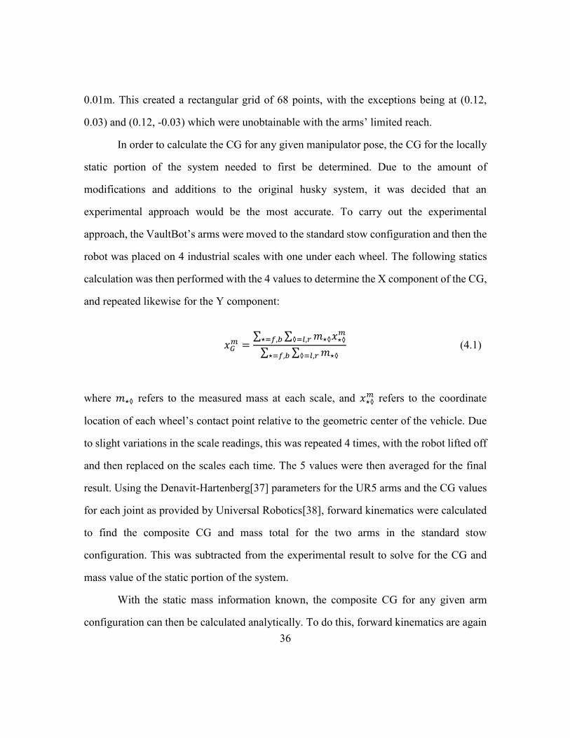
36
0.01m. This created a rectangular grid of 68 points, with the exceptions being at (0.12,
0.03) and (0.12, -0.03) which were unobtainable with the arms’ limited reach.
In order to calculate the CG for any given manipulator pose, the CG for the locally
static portion of the system needed to first be determined. Due to the amount of
modifications and additions to the original husky system, it was decided that an
experimental approach would be the most accurate. To carry out the experimental
approach, the VaultBot’s arms were moved to the standard stow configuration and then the
robot was placed on 4 industrial scales with one under each wheel. The following statics
calculation was then performed with the 4 values to determine the X component of the CG,
and repeated likewise for the Y component:
𝑥𝐺𝑚 =
∑ ∑ 𝑚⋆◊𝑥⋆◊𝑚
◊=𝑙,𝑟⋆=𝑓,𝑏
∑ ∑ 𝑚⋆◊◊=𝑙,𝑟⋆=𝑓,𝑏 (4.1)
where 𝑚⋆◊ refers to the measured mass at each scale, and 𝑥⋆◊𝑚 refers to the coordinate
location of each wheel’s contact point relative to the geometric center of the vehicle. Due
to slight variations in the scale readings, this was repeated 4 times, with the robot lifted off
and then replaced on the scales each time. The 5 values were then averaged for the final
result. Using the Denavit-Hartenberg[37] parameters for the UR5 arms and the CG values
for each joint as provided by Universal Robotics[38], forward kinematics were calculated
to find the composite CG and mass total for the two arms in the standard stow
configuration. This was subtracted from the experimental result to solve for the CG and
mass value of the static portion of the system.
With the static mass information known, the composite CG for any given arm
configuration can then be calculated analytically. To do this, forward kinematics are again

37
utilized to find the CG and mass values of the dynamic components which are then added
to the static values. Obtaining a configuration which resulted in the desired CG location
for each test was then simply a matter of manually moving the arms, updating the CG
calculation, and repeating until sufficiently close. The large discrepancy in degrees of
freedom between the dynamic elements (12, in the two mobile manipulators) and the
desired output (3, CG position) results in a near-infinite number of solutions for any desired
CG position, which encouraged the manual approach.
4.2.1.3. Center-of-Rotation
To find the CoR given an arc trajectory, the start and final points of the trajectory
are mapped with a rotation matrix based on the change in heading:
[𝑥𝑓 − 𝑐𝑥
𝑦𝑓 − 𝑐𝑦] = [
𝑐Δ𝜃 −𝑠Δ𝜃𝑠Δ𝜃 𝑐Δ𝜃
] [𝑥𝑠 − 𝑐𝑥
𝑦𝑠 − 𝑐𝑦] (4.2)
𝛥𝜃 = 𝜃𝑓 − 𝜃𝑠, 𝜃𝑠 = 0, ∴ 𝛥𝜃 = 𝜃𝑓 = 𝜃 (4.3)
where the position and heading data for the start point is represented as (𝑥𝑠, 𝑦𝑠, 𝜃𝑠)., and
the data for the final point is given as (𝑥𝑓 , 𝑦𝑓 , 𝜃𝑓). Then solving for the CoR coordinates
(𝑐𝑥, 𝑐𝑦) gives:
𝑥𝑓 − 𝑐𝑥 = 𝑐𝜃(𝑥𝑠 − 𝑐𝑥) − 𝑠𝜃(𝑦𝑠 − 𝑐𝑦), 𝑦𝑓 − 𝑐𝑦 = 𝑠𝜃(𝑥𝑠 − 𝑐𝑥) + 𝑠𝜃(𝑦𝑠 − 𝑐𝑦)
𝑐𝑥 = −𝑥𝑓 + 𝑥𝑠 − 𝑥𝑓𝑐𝜃 − 𝑥𝑠𝑐𝜃 − 𝑦𝑓𝑠𝜃 + 𝑦𝑠𝑠𝜃
2(𝑐𝜃 − 1) (4.4)
𝑐𝑦 = −𝑦𝑓 + 𝑦𝑠 − 𝑦𝑓𝑐𝜃 − 𝑦𝑠𝑐𝜃 + 𝑥𝑓𝑠𝜃 − 𝑥𝑠𝑠𝜃
2(𝑐𝜃 − 1) (4.5)
38
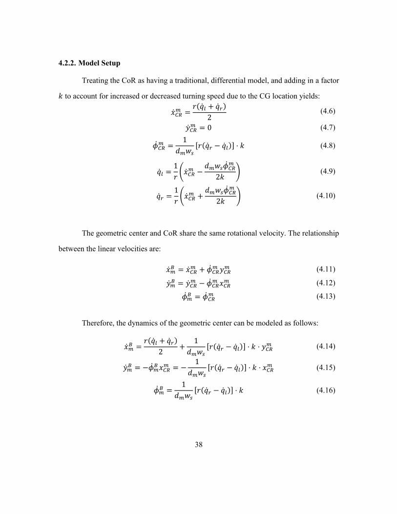
4.2.2. Model Setup
Treating the CoR as having a traditional, differential model, and adding in a factor
𝑘 to account for increased or decreased turning speed due to the CG location yields:
�̇�𝐶𝑅𝑚 =
𝑟(�̇�𝑙 + �̇�𝑟)
2 (4.6)
�̇�𝐶𝑅𝑚 = 0 (4.7)
�̇�𝐶𝑅𝑚 =
1
𝑑𝑚𝑤𝑠
[𝑟(�̇�𝑟 − �̇�𝑙)] ⋅ 𝑘 (4.8)
�̇�𝑙 =1
𝑟(�̇�𝐶𝑅
𝑚 −𝑑𝑚𝑤𝑠�̇�𝐶𝑅
𝑚
2𝑘) (4.9)
�̇�𝑟 =1
𝑟(�̇�𝐶𝑅
𝑚 +𝑑𝑚𝑤𝑠�̇�𝐶𝑅
𝑚
2𝑘) (4.10)
The geometric center and CoR share the same rotational velocity. The relationship
between the linear velocities are:
�̇�𝑚𝐵 = �̇�𝐶𝑅
𝑚 + �̇�𝐶𝑅𝑚 𝑦𝐶𝑅
𝑚 (4.11)
�̇�𝑚𝐵 = �̇�𝐶𝑅
𝑚 − �̇�𝐶𝑅𝑚 𝑥𝐶𝑅
𝑚 (4.12)
�̇�𝑚𝐵 = �̇�𝐶𝑅
𝑚 (4.13)
Therefore, the dynamics of the geometric center can be modeled as follows:
�̇�𝑚𝐵 =
𝑟(�̇�𝑙 + �̇�𝑟)
2+
1
𝑑𝑚𝑤𝑠
[𝑟(�̇�𝑟 − �̇�𝑙)] ⋅ 𝑘 ⋅ 𝑦𝐶𝑅𝑚 (4.14)
�̇�𝑚𝐵 = −�̇�𝑚
𝐵 𝑥𝐶𝑅𝑚 = −
1
𝑑𝑚𝑤𝑠
[𝑟(�̇�𝑟 − �̇�𝑙)] ⋅ 𝑘 ⋅ 𝑥𝐶𝑅𝑚 (4.15)
�̇�𝑚𝐵 =
1
𝑑𝑚𝑤𝑠
[𝑟(�̇�𝑟 − �̇�𝑙)] ⋅ 𝑘 (4.16)

39
Note that since �̇�𝑚𝐵 is non-zero, the system is now overdetermined. To solve for the
wheel speeds therefore, only equations 4.14 and 4.16 are utilized:
�̇�𝑙 =1
𝑟(�̇�𝑚
𝐵 − �̇�𝑚𝐵 𝑦𝐶𝑅
𝑚 −�̇�𝑚
𝐵 𝑑𝑚𝑤𝑠
2𝑘) (4.17)
�̇�𝑟 =1
𝑟(�̇�𝑚
𝐵 − �̇�𝑚𝐵 𝑦𝐶𝑅
𝑚 +�̇�𝑚
𝐵 𝑑𝑚𝑤𝑠
2𝑘) (4.18)
Given the circumstances, this is the most logical solution to the overdetermined
system. Out of the three possible control inputs only two can be utilized, and �̇�𝑚𝐵 and �̇�𝑚
𝐵
are the two most intuitive control inputs from an operator’s perspective. However, this also
reveals the inherent challenge with controlling the VaultBot platform. As long as 𝑥𝐶𝑅𝑚 is
non-zero �̇�𝑚𝐵 is also non-zero, and if �̇�𝑚
𝐵 is non-zero then the system is not fully controllable.
Therefore, while steps such those described in this section can be made to improve the
model, perfect open-loop trajectory tracking is unattainable.
4.2.3. Results
As the tests were performed, all relevant data was logged using the rosbag utility
and then post-processed, analyzed, and plotted using python. The in-place rotation tests

40
immediately demonstrated significant variance in the VaultBot’s behavior dependent on
the position of its CG.
Figure 4-2: In-Place Rotation Position Tracking, COM-y position @ 0.02
Figure 4-2 shows a sample of 10 of the 68 tested CG locations, in this case with the
Y-coordinate held constant at 0.02m, and the X-coordinate varied from -0.06m to 0.12m.
41
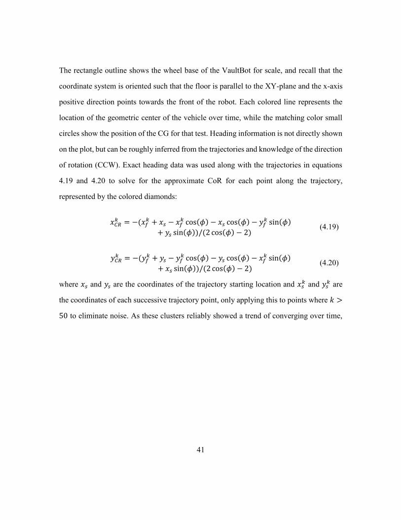
The rectangle outline shows the wheel base of the VaultBot for scale, and recall that the
coordinate system is oriented such that the floor is parallel to the XY-plane and the x-axis
positive direction points towards the front of the robot. Each colored line represents the
location of the geometric center of the vehicle over time, while the matching color small
circles show the position of the CG for that test. Heading information is not directly shown
on the plot, but can be roughly inferred from the trajectories and knowledge of the direction
of rotation (CCW). Exact heading data was used along with the trajectories in equations
4.19 and 4.20 to solve for the approximate CoR for each point along the trajectory,
represented by the colored diamonds:
𝑥𝐶𝑅
𝑘 = −(𝑥𝑓𝑘 + 𝑥𝑠 − 𝑥𝑓
𝑘 cos(𝜙) − 𝑥𝑠 cos(𝜙) − 𝑦𝑓𝑘 sin(𝜙)
+ 𝑦𝑠 sin(𝜙))/(2 cos(𝜙) − 2) (4.19)
𝑦𝐶𝑅
𝑘 = −(𝑦𝑓𝑘 + 𝑦𝑠 − 𝑦𝑓
𝑘 cos(𝜙) − 𝑦𝑠 cos(𝜙) − 𝑥𝑓𝑘 sin(𝜙)
+ 𝑥𝑠 sin(𝜙))/(2 cos(𝜙) − 2) (4.20)
where 𝑥𝑠 and 𝑦𝑠 are the coordinates of the trajectory starting location and 𝑥𝑠𝑘 and 𝑦𝑠
𝑘 are
the coordinates of each successive trajectory point, only applying this to points where 𝑘 >
50 to eliminate noise. As these clusters reliably showed a trend of converging over time,

42
the final point was selected as the CoR for the whole trajectory, and was highlighted using
a larger circle of the appropriate color.
Figure 4-3: In-Place Rotation Smoothed Angular Velocities, COM-y position @ -0.03
The rotational velocity for each test was also calculated by dividing the change in
heading data by the sample time for each interval, and then smoothing the result with a

43
moving average. Figure 4-3 shows the results for the set of tests with a constant Y-
coordinate value of -0.03m. This shows that, after an initial acceleration, each trajectory
maintains a fairly consistent velocity over time. The values from these plateaus were then
averaged to find an approximation for the whole trajectory’s average rotational velocity.
Table 4-1: Average Rotational Velocity Ratio to Cmd. Velocity
The average rotational velocity values were then divided by the command velocity
of 0.3 rad/s to obtain an error ratio and then tabulated, as seen in Table 4-1.
0.3 CG_x -0.06 -0.04 -0.02 0 0.02 0.04 0.06 0.08 0.1 0.12
CG_y Avg Std. Dev.
0.03 1.120 1.023 0.963 0.947 0.960 1.017 1.087 1.247 1.443 1.090 0.163
0.02 1.107 1.020 0.977 0.963 0.977 1.013 1.090 1.283 1.500 1.603 1.153 0.231
0.01 1.120 1.027 0.980 0.967 0.983 1.037 1.117 1.273 1.480 1.607 1.159 0.224
0 1.120 1.027 0.987 0.973 0.983 1.033 1.113 1.290 1.480 1.597 1.160 0.222
-0.01 1.120 1.037 0.987 0.970 0.980 1.013 1.097 1.280 1.533 1.620 1.164 0.237
-0.02 1.117 1.017 0.970 0.960 0.977 1.013 1.103 1.267 1.503 1.607 1.153 0.232
-0.03 1.107 1.013 0.970 0.960 0.970 0.993 1.097 1.273 1.500 1.098 0.181
Avg 1.116 1.023 0.976 0.963 0.976 1.017 1.100 1.273 1.491 1.607
Std. Dev. 0.006 0.008 0.009 0.009 0.008 0.014 0.011 0.014 0.028 0.008
Avg
. Rot
. Vel
ocit
y R
atio
to
Cm
d.

44
Figure 4-4: Average Rotational Velocity Error Ratios vs. CG position
Figure 4-5: Average Rotational Velocity Error Ratios vs. CG x-position
The error ratios were then plotted against their CG position in Figure 4-4. This
indicates a strong dependence on the x-coordinate and independence with the y-coordinate
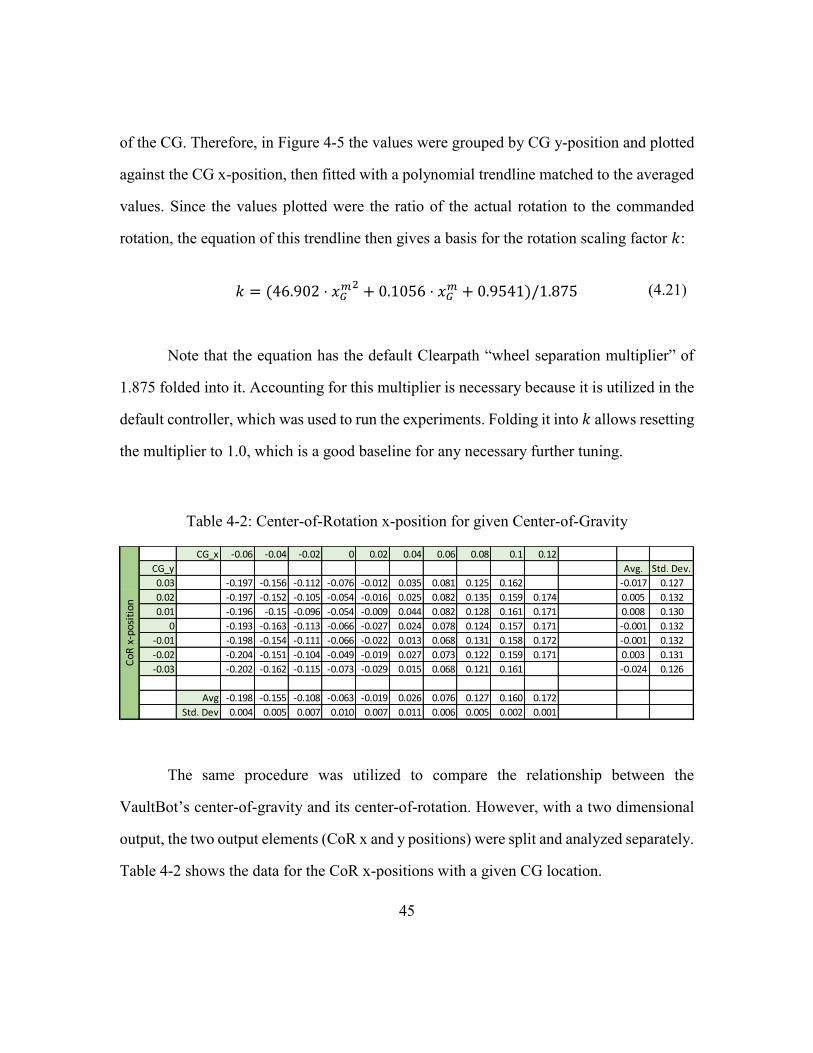
45
of the CG. Therefore, in Figure 4-5 the values were grouped by CG y-position and plotted
against the CG x-position, then fitted with a polynomial trendline matched to the averaged
values. Since the values plotted were the ratio of the actual rotation to the commanded
rotation, the equation of this trendline then gives a basis for the rotation scaling factor 𝑘:
𝑘 = (46.902 ⋅ 𝑥𝐺𝑚2
+ 0.1056 ⋅ 𝑥𝐺𝑚 + 0.9541)/1.875 (4.21)
Note that the equation has the default Clearpath “wheel separation multiplier” of
1.875 folded into it. Accounting for this multiplier is necessary because it is utilized in the
default controller, which was used to run the experiments. Folding it into 𝑘 allows resetting
the multiplier to 1.0, which is a good baseline for any necessary further tuning.
Table 4-2: Center-of-Rotation x-position for given Center-of-Gravity
The same procedure was utilized to compare the relationship between the
VaultBot’s center-of-gravity and its center-of-rotation. However, with a two dimensional
output, the two output elements (CoR x and y positions) were split and analyzed separately.
Table 4-2 shows the data for the CoR x-positions with a given CG location.
CG_x -0.06 -0.04 -0.02 0 0.02 0.04 0.06 0.08 0.1 0.12
CG_y Avg. Std. Dev.
0.03 -0.197 -0.156 -0.112 -0.076 -0.012 0.035 0.081 0.125 0.162 -0.017 0.127
0.02 -0.197 -0.152 -0.105 -0.054 -0.016 0.025 0.082 0.135 0.159 0.174 0.005 0.132
0.01 -0.196 -0.15 -0.096 -0.054 -0.009 0.044 0.082 0.128 0.161 0.171 0.008 0.130
0 -0.193 -0.163 -0.113 -0.066 -0.027 0.024 0.078 0.124 0.157 0.171 -0.001 0.132
-0.01 -0.198 -0.154 -0.111 -0.066 -0.022 0.013 0.068 0.131 0.158 0.172 -0.001 0.132
-0.02 -0.204 -0.151 -0.104 -0.049 -0.019 0.027 0.073 0.122 0.159 0.171 0.003 0.131
-0.03 -0.202 -0.162 -0.115 -0.073 -0.029 0.015 0.068 0.121 0.161 -0.024 0.126
Avg -0.198 -0.155 -0.108 -0.063 -0.019 0.026 0.076 0.127 0.160 0.172
Std. Dev 0.004 0.005 0.007 0.010 0.007 0.011 0.006 0.005 0.002 0.001
CoR
x-p
osit
ion

46
Figure 4-6: Center-of-Rotation x-position vs. Center-of-Gravity position
Figure 4-7: Center-of-Rotation x-position vs. Center-of-Gravity x-position
y = 2.1722x - 0.0635R² = 0.9931
-0.25
-0.2
-0.15
-0.1
-0.05
0
0.05
0.1
0.15
0.2
0.25
-0.08 -0.06 -0.04 -0.02 0 0.02 0.04 0.06 0.08 0.1 0.12 0.14
CoR x-position vs. CG x-position (m)
0.03 0.02 0.01 0 -0.01 -0.02 -0.03 Average

47
Similarly to the rotational velocity analysis, the 3D chart given in Figure 4-6 shows
a strong dependence of the CoR’s x-coordinate with the CG x-position, and a strong
independence from the CG y-position. Therefore, a simple heuristic equation can be
extracted from the trendline in Figure 4-7 to solve for the x-coordinate of the CoR:
𝑥𝐶𝑅𝑚 = 2.1722 ⋅ 𝑥𝐺
𝑚 − 0.0635 (4.22)
Table 4-3: Center-of-Rotation y-position for given Center-of-Gravity
CG_x -0.06 -0.04 -0.02 0 0.02 0.04 0.06 0.08 0.1 0.12
CG_y Avg. Std. Dev.
0.03 -0.021 -0.04 -0.056 -0.05 -0.049 -0.05 -0.046 -0.043 -0.032 -0.043 0.011
0.02 -0.015 -0.022 -0.032 -0.032 -0.04 -0.045 -0.053 -0.039 -0.022 -0.01 -0.031 0.014
0.01 0.009 -0.007 -0.014 -0.012 -0.029 -0.038 -0.039 -0.039 -0.014 -0.007 -0.019 0.016
0 0.01 0.009 0.008 0.001 -0.006 -0.015 -0.017 -0.023 -0.022 -0.01 -0.007 0.013
-0.01 0.027 0.021 0.017 0.015 0.012 0.006 0.007 -0.001 -0.008 -0.004 0.009 0.011
-0.02 0.051 0.034 0.037 0.03 0.026 0.026 0.013 0.004 -0.01 -0.005 0.021 0.020
-0.03 0.048 0.053 0.046 0.047 0.044 0.039 0.02 0.012 -0.003 0.034 0.020
Avg 0.016 0.007 0.001 0.000 -0.006 -0.011 -0.016 -0.018 -0.016 -0.007
Std. Dev 0.028 0.032 0.037 0.034 0.035 0.036 0.030 0.023 0.010 0.003
CoR
y-p
osit
ion

48
Figure 4-8: Center-of-Rotation y-coordinate vs. Center-of-Gravity location
Figure 4-9: Center-of-Rotation y-coordinate vs. Center-of-Gravity x-coordinate

49
Figure 4-10: Center-of-Rotation y-position vs. Center-of-Gravity y-position
As can been seen in Table 4-3 and Figure 4-8 - Figure 4-10, the relationship
between the CoR y-coordinate and the CG location is not as simple as previously examined
correlations. At this point, due to the apparent dependence on two variables rather than just
one, several approaches were taken. The first approach was to utilize the built-in
multivariate regression analysis from Microsoft Excel [39].
Table 4-4: Multivariate Regression of CoR y-position for given CG, part 1
Regression Statistics
Multiple R 0.92588449
R Square 0.857262088
Adjusted R Square 0.852870153
Standard Error 0.011301514
Observations 68

50
Table 4-5: Multivariate Regression of CoR y-position for given CG, part 2
Table 4-6: Multivariate Regression of CoR y-position for given CG, part 3
Figure 4-11: Multivariate Regression of CoR y-position for given CG; Results
At first glance, a very low significance F value (Table 4-5) and decent R values
(Table 4-4) indicate that the multivariate regression is a good fit for the data. The
coefficients in Table 4-6 then result in the following equation solving for the y-coordinate
of the CoR:
𝑦𝐶𝑅𝑚 = −0.166 ⋅ 𝑥𝐺
𝑚 − 1.295 ⋅ 𝑦𝐺𝑚 − 0.0006 (4.23)
ANOVA
df SS MS F Significance F
Regression 2 0.049860985 0.02493 195.190034 3.33065E-28
Residual 65 0.008302074 0.000128
Total 67 0.058163059
Coefficients Standard Error t Stat P-value Lower 95% Upper 95% Lower 95.0% Upper 95.0%
Intercept -0.000571511 0.001524523 -0.37488 0.70897122 -0.003616194 0.002473172 -0.003616194 0.002473172
CG_x -0.166202827 0.024411906 -6.80827 3.7791E-09 -0.214956769 -0.117448885 -0.214956769 -0.117448885
CG_y -1.295038168 0.069820984 -18.548 1.1692E-27 -1.434480302 -1.155596034 -1.434480302 -1.155596034

51
However, when observing Figure 4-11 it becomes clear that the regression does a
poor job of modeling the convergence of the CoR y-coordinate to zero when the CG x-
coordinate increases to 0.12. The orange markers indicate the predicted CoR y-values given
the fixed inputs using the regression model, while the blue markers show the
experimentally measured positions.
A second approach was a two-step method leveraging the apparent linearity of the
data sets in Figure 4-10. As is shown, each data set was fit with a linear trendline.
Table 4-7: Equation Coefficients for Linear Regression of Figure 4-10 data
The coefficients of the linear trendlines were then tabulated based on the CG x-
position, which was the feature that differentiated the data sets in Figure 4-10. These
coefficients were then plotted separately against the CG x-position and fit with polynomial
trendlines of their own:
CG-x -0.06 -0.04 -0.02 0 0.02 0.04 0.06 0.08 0.1 0.12
Slope -1.275 -1.4964 -1.6964 -1.5786 -1.6143 -1.6179 -1.3429 -1.0321 -0.4179 -0.13
Intercept 0.0156 0.0069 0.0009 -0.0001 -0.006 -0.011 -0.0164 -0.0184 -0.0159 -0.0072
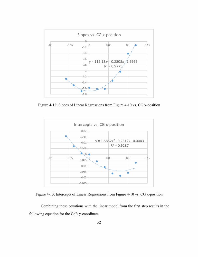
52
Figure 4-12: Slopes of Linear Regressions from Figure 4-10 vs. CG x-position
Figure 4-13: Intercepts of Linear Regressions from Figure 4-10 vs. CG x-position
Combining these equations with the linear model from the first step results in the
following equation for the CoR y-coordinate:

53
𝑦𝐶𝑅
𝑚 = (115.18 ⋅ 𝑥𝐺𝑚2
− 0.2808 ⋅ 𝑥𝐺𝑚 − 1.6955) ⋅ 𝑦𝐺
𝑚
+ (1.5852 ⋅ 𝑥𝐺𝑚2
− 0.2512 ⋅ 𝑥𝐺𝑚 − 0.0043)
(4.24)
This model results in a significantly better mapping to the observed data, as can be
seen in Figure 4-14.
Figure 4-14: Predicted vs. Measured CoR y-position with Full Model
However, the model also reveals a bias to one side which is due to either the
direction of rotation, or un-modeled asymmetry in the VaultBot’s behavior, perhaps due to
the arrangement of the tire treads. In the interest of a more general solution, and since clean
measurements of the other direction of rotation are unfeasible as previously discussed,
another model was developed to remove the asymmetry.
𝑦𝐶𝑅𝑚 = (115.18 ⋅ 𝑥𝐺
𝑚2− 0.2808 ⋅ 𝑥𝐺
𝑚 − 1.6955) ⋅ 𝑦𝐺𝑚 (4.25)
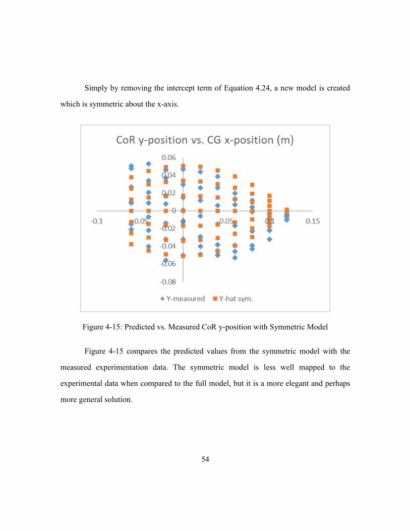
54
Simply by removing the intercept term of Equation 4.24, a new model is created
which is symmetric about the x-axis.
Figure 4-15: Predicted vs. Measured CoR y-position with Symmetric Model
Figure 4-15 compares the predicted values from the symmetric model with the
measured experimentation data. The symmetric model is less well mapped to the
experimental data when compared to the full model, but it is a more elegant and perhaps
more general solution.

55
4.3. CONCLUSIONS & IMPLEMENTATION
From simple observation of the VaultBot’s behavior, it seems intuitive that the
vehicle rotates about the location of its CG when attempting an in-place rotation. However,
analysis of the experimental data reveals this is not the case. Equation 4.22 shows that the
x-coordinate of the CoR scales linearly with the CG x-coordinate, along with having a
constant offset. The scaling factor reflects the complex slip interactions resulting from the
shifting normal forces, and its sign concurs with logical intuition; if the CG were to
coincide with either the front or rear axis, the VaultBot would be expected to behave like
a differentially steered vehicle at that axis, with the other axis having very little effect on
the motion. This would also suggest that the linear model would break down as the CG
approaches these extremes, and close analysis of Figure 4-7 shows that this may be the
case, with all points at 𝑥𝐺𝑚 = 0.012 beginning to tail off below the trendline. Within the
operational reach of the manipulators however, the linear model holds strong. The constant
offset likely reflects the rotational inertia of the mobile manipulator. Due to the forward
positioning of the arm mount locations, a configuration which results in a forward shift of
the CG tends to have a higher rotational inertia than a configuration resulting in an
equivalent backwards shift. Further study to better understand the rotational inertia’s effect
on the system’s behavior is warranted.
Figure 4-5 also shows that as the CG shifts forward or backwards towards the
extremes, the angular velocity of the VaultBot increases. The reason for this is intuitive.
As the mass becomes unbalanced towards one end of the vehicle, the slips in the wheels at
that end decrease until they are theoretically zero, when the mass is directly centered over
the axis and the dynamic model matches that of a differentially steered platform.
Conversely, the decrease in normal forces at the opposing end leads to a significant increase

56
in slip and decrease in lateral friction, until the extreme case when there is theoretically no
lateral friction at all to oppose the rotational motion imposed by the primary wheel axis.
Somewhat counterintuitively, the y-coordinate of the center-of-rotation scales
inversely with the y-coordinate of the center-of-gravity. Once again consideration of the
extreme case, here with the CG directly aligned with either the left or right wheels, clarifies
the behavior.
Figure 4-16: CoR behavior with varying CG y-coordinate
Alignment with the left wheels is the situation considered in Figure 4-16, part A.
In this ideal case, the normal forces on the opposite wheels would be zero and the vehicle

57
would travel straight, only having driving contribution from the left set of wheels. Thus,
the CoR would exist at ±∞, and the system would behave much like a bicycle with a fixed
steering column. However, since the CoR can exist at either positive or negative infinity,
this does not clarify the relationship between it and the CG. For that, we consider the case
in Figure 4-16, part B. Here we have moved the CG ever so slightly to the right, to the
inside of the left wheels. This introduces very small normal force interactions at the right
wheels which we treat as negligible as to continue the bicycle analogy. A bicycle with a
fixed steering column and a slightly offset center of gravity will gradually turn to that side,
so we can identify the CoR’s location to be at some large, positive value that is less than
infinity. Therefore, it appears that the CG and CoR trend in opposite directions and come
to their logical conclusion in part C, the most basic case where they are coincident and the
vehicle exhibits ideal in-place rotation. Nevertheless, within the operating range of the
manipulators the differential behavior resulting from a forward or backward shift in the CG
is the dominating factor. The effect of the y-coordinate of the CG is greatly diminished
when the x-coordinate is largely positive or negative.
To implement these heuristic equations, a new ros_control package was
created named skid_steer_controller, closely derived from
diff_drive_controller. The controller was expanded to allow for y-velocity
tracking in the odometry, and Equations 4.14-4.18 were utilized to replace the primary
odometry and wheel speed calculations. Equations 4.21-4.22 were implemented to solve
for new parameters 𝑘 and 𝑥𝐶𝑅𝑚 , respectively, while Equations 4.23-4.25 were utilized to
solve for 𝑦𝐶𝑅𝑚 subject to an adjustable selection parameter, with the default set to Equation
4.25 which is most consistent with the symmetry assumption discussed in Section 5.2.1.

58
Chapter 5: Demonstration
5.1. SETUP
In order to experimentally validate the new controller, a rigorous set of experiments
with varying CG positions and varying command trajectories was devised. 7 different arm
configurations and 6 different open-loop trajectories were combined for a total of 42
experiments, with the goal of obtaining a sufficiently representative spread of CG positions
and dynamic scenarios. This set of experiments was also run twice, once with the default
diff_drive_controller, and once with the new skid_steer_controller for
a grand total of 84 experiments.
Figure 5-1: Centers of Gravity for Controller Tests

59
The resultant centers of gravity from the 7 arm configurations are shown in Figure
5-1, while the trajectories consisted of a simple in-place rotation:
“Rotate” 𝑣𝑥 = 0 𝑚/𝑠
�̇� = 0.3 𝑟𝑎𝑑/𝑠} 𝑓𝑜𝑟 0 < 𝑡 < 5.0𝑠 (5.1)
an “S-curve” trajectory, with a constant forward velocity and a sinusoidal rotational
velocity:
“S-curve”
𝑣𝑥 = 0.4 𝑚/𝑠
�̇� = 0.5 ∗ sin (2𝜋𝑡
9.0) 𝑟𝑎𝑑/𝑠
} 𝑓𝑜𝑟 0 < 𝑡 < 10.0𝑠 (5.2)
And 4 distinct “Arc” behaviors, with constant linear and rotational velocities:
“Arc #1” 𝑣𝑥 = 0.5 𝑚/𝑠
�̇� = 0.1 𝑟𝑎𝑑/𝑠} 𝑓𝑜𝑟 0 < 𝑡 < 6.0𝑠 (5.3)
“Arc #2” 𝑣𝑥 = 0.5 𝑚/𝑠
�̇� = −0.1 𝑟𝑎𝑑/𝑠} 𝑓𝑜𝑟 0 < 𝑡 < 6.0𝑠 (5.4)
“Arc #3” 𝑣𝑥 = 0.5 𝑚/𝑠
�̇� = 0.5 𝑟𝑎𝑑/𝑠} 𝑓𝑜𝑟 0 < 𝑡 < 3.0𝑠 (5.5)
“Arc #4” 𝑣𝑥 = −0.5 𝑚/𝑠
�̇� = 0.1 𝑟𝑎𝑑/𝑠} 𝑓𝑜𝑟 0 < 𝑡 < 6.0𝑠 (5.6)
These tests were again performed on the same smooth concrete floor as the data
collection tests, in the Nuclear and Applied Robotics Group lab facilities at JJ Pickle
Research Campus. Also, Hector SLAM was again used to track the VaultBot’s actual
location over time (see Section 4.2.1.1), and data was collected and processed in ROS
bagfiles.

60
5.2. RESULTS
In order to qualitatively compare the two controllers, each of the 42 CG-position
and trajectory combinations was given its own graph, plotting the true trajectories against
the calculated trajectories for each controller as well as the intended open-loop command
trajectory. The latter was derived by leveraging a pre-existing “updateOpenLoop” method
in the diff_drive_controller, which simply integrates an input of linear and
angular velocities (Equations 5.1-5.6) with the timestep to update a trajectory.
Figure 5-2: Controller Odometry in Scurve Front Left Configuration

61
Figure 5-2 is a clearly interpreted example, showing the case with the arms (and
thus the CG) in the front left position and traversing the s-curve trajectory. The rectangle
in the bottom left of the figure represents the wheelbase of the VaultBot in its starting
configuration. The dark teal circle represents the CG location, while the faded teal diamond
shows the approximate CoR in an in-place rotation case, as derived in Section 4.2. The
gray line is the intended open-loop command, while the solid orange and teal lines are the
actual paths traveled under the diff_drive_controller and the
skid_steer_controller, respectively. The odometry output from each controller is
shown by the dotted lines. Figure 5-3 -Figure 5-5 show more examples in varying CG-
trajectory combinations.
Figure 5-3: Controller Odometry in Arc #2 Back Right Configuration

62
Figure 5-4: Controller Odometry in Rotate Ready Configuration

63
Figure 5-5: Controller Odometry in Arc #4 Ready Back Configuration
From these four examples alone, it is clear that there is significant variation in the
controller performance. Therefore, in order to properly evaluate the performance, it was
necessary to benchmark each configuration against a set of criteria. Particularly in the case
of skid-steer or other insufficiently modeled mobile bases, there are two significant areas
of open-loop error that closed-loop methods must overcome. The first is when the
autonomous agent thinks, via odometry, that it is somewhere it is not. This is represented
in the figures above by the difference between the solid and dotted lines. The greater this
error, the more correction that is necessary from any closed-loop localization methods such
as laser scan based particle filtering or landmark detection. The second area is when the
autonomous agent goes somewhere other than where it was commanded to go. This is
represented by the error between the colored solid lines and the solid gray line. The greater
this error, the more correction that is necessary from closed-loop navigation controllers,
continuously fighting the actual behavior of the robot to try and keep it on course.
Therefore, each configuration was qualitatively analyzed to evaluate whether the
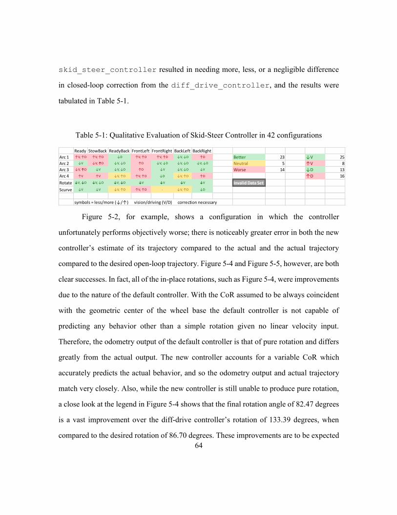
64
skid_steer_controller resulted in needing more, less, or a negligible difference
in closed-loop correction from the diff_drive_controller, and the results were
tabulated in Table 5-1.
Table 5-1: Qualitative Evaluation of Skid-Steer Controller in 42 configurations
Figure 5-2, for example, shows a configuration in which the controller
unfortunately performs objectively worse; there is noticeably greater error in both the new
controller’s estimate of its trajectory compared to the actual and the actual trajectory
compared to the desired open-loop trajectory. Figure 5-4 and Figure 5-5, however, are both
clear successes. In fact, all of the in-place rotations, such as Figure 5-4, were improvements
due to the nature of the default controller. With the CoR assumed to be always coincident
with the geometric center of the wheel base the default controller is not capable of
predicting any behavior other than a simple rotation given no linear velocity input.
Therefore, the odometry output of the default controller is that of pure rotation and differs
greatly from the actual output. The new controller accounts for a variable CoR which
accurately predicts the actual behavior, and so the odometry output and actual trajectory
match very closely. Also, while the new controller is still unable to produce pure rotation,
a close look at the legend in Figure 5-4 shows that the final rotation angle of 82.47 degrees
is a vast improvement over the diff-drive controller’s rotation of 133.39 degrees, when
compared to the desired rotation of 86.70 degrees. These improvements are to be expected
Ready StowBack ReadyBack FrontLeft FrontRight BackLeft BackRight
Arc 1 ↑V, ↑D ↑V, ↑D ↓D ↑V, ↑D ↑V, ↑D ↓V, ↓D ↑D Better 23 ↓V 25
Arc 2 ↓V ↓V, ↑D ↓V, ↓D ↑D ↓V, ↓D ↓V, ↓D ↓V, ↓D Neutral 5 ↑V 8
Arc 3 ↓V, ↑D ↓V ↓V, ↓D ↑D ↓V ↓V, ↓D ↓V Worse 14 ↓D 13
Arc 4 ↑V ↑V ↓V, ↑D ↑V, ↑D ↓D ↓V, ↑D ↑D ↑D 16
Rotate ↓V, ↓D ↓V, ↓D ↓V, ↓D ↓V ↓V ↓V ↓V Invalid Data Set
Scurve ↓V ↓V ↓V, ↑D ↑V, ↑D - ↓V, ↑D ↓D
symbols = less/more (↓/↑) vision/driving (V/D) correction necessary

65
however, as the in-place rotation trajectory was the basis for the skid-steer controller
derivations. In 23 of the 42 configurations, the skid-steer controller was a noticeable
improvement over the default controller. In 5 configurations it had a neutral impact and
either showed a negligible difference or offset between the two criteria. However, in the
other 14 cases the new controller performed noticeably worse. Also of note is that when
the controller showed an improvement, it tended to decrease the vision correction
necessary; i.e. the VaultBot was more accurate in its approximation of where it was
throughout the trajectory. Conversely, it performed worse more often in the area of driving
correction and would deviate further from the desired open-loop trajectory that the skid-
steer controller.
In order to validate the qualitative analysis, a quantitative approach was taken as
well. For the driving comparisons, that is the actual robot path versus the desired open loop
trajectory, two approaches were utilized. First was a direct comparison of the trajectories,
which was done by resampling the trajectories into an equal number of points, calculating
the Euclidean distance between each pair of points, and averaging the result. The lower the
average “drive error”, the better the result. However, this by itself would only tell part of
the story; one could conceivably have a controller with a widely varying trajectory that
ends up very close to the desired end goal, or one that very slightly but consistently deviates
from the desired trajectory to end up far from the goal. Therefore, a second metric was
included to evaluate the end positions. Rather than a simple Euclidean distance, however,
the metric was the requisite time for position correction. This was to account for the fact
that deviation in the x-direction is much easier to correct than deviation in the y-direction
due to the platform’s non-holonomic nature and aversion to in-place rotations. “Correction
time” was calculated with 3 phases: turning towards the goal, driving linearly to the goal,

66
and then rotating again to the correct orientation. The requisite angles of rotation were
divided by the appropriate average rotational velocities for each arm configuration, which
were determined using the known CGs, Equation 4.21, and the in-place rotation control
velocity of 0.3 rad/s. The linear translation was divided by the standard linear velocity of
0.5 m/s. For odometry comparisons, that is the actual robot path versus the calculated robot
path with odometry, only the trajectory comparison technique was utilized. Since the
correcting measures for this error typically rely on continuous correction from closed-loop
vision systems, the trajectory evaluation result was referred to as “vision error”. Also for
this reason the end position correction technique was deemed to not provide additional
insight and was omitted. The quantitative results are presented in Table 5-2 below.
Table 5-2: Quantitative Evaluation of Skid-Steer Controller in 42 configurations
Skid Diff Skid Diff Skid Diff Skid Diff Skid Diff Skid Diff Skid Diff
Drive Error (m) 0.122 0.026 0.034 0.015 0.027 0.047 0.049 0.02 0.052 0.019 0.027 0.046 0.023 0.02
Correction Time(s) 4.03 1.628 3.105 1.277 4.638 3.19 2.154 0.554 3.108 1.119 1.525 3.033 1.595 0.939
Vision Error (m) 0.073 0.031 0.024 0.016 0.073 0.057 0.034 0.015 0.029 0.021 0.019 0.053 0.011 0.021
Drive Error (m) 0.069 0.046 0.038 0.027 0.011 0.065 0.045 0.015 0.031 0.015 0.026 0.036 0.025 0.049
Correction Time(s) 3 3.235 3.287 2.835 0.831 4.534 3.99 2.096 1.084 1.901 1.658 2.743 1.959 3.478
Vision Error (m) 0.038 0.047 0.021 0.036 0.056 0.069 0.025 0.016 0.019 0.018 0.022 0.039 0.013 0.055
Drive Error (m) 0.108 0.055 0.027 0.028 0.055 0.1 0.058 0.034 0.044 0.041 0.032 0.051 0.039 0.033
Correction Time(s) 2.726 2.381 3.12 3.316 2.522 3.495 3.585 3.299 2.989 2.889 3.266 3.179 2.963 3.008
Vision Error (m) 0.017 0.056 0.014 0.035 0.031 0.101 0.029 0.034 0.017 0.038 0.023 0.055 0.025 0.042
Drive Error (m) 0.072 0.061 0.018 0.026 0.066 0.042 0.052 0.012 0.024 0.045 0.05 0.051 0.046 0.027
Correction Time(s) 2.634 3.491 1.318 0.698 3.129 1.039 2.211 0.969 1.081 2.539 2.29 1.577 1.784 0.708
Vision Error (m) 0.127 0.064 0.02 0.02 0.031 0.037 0.057 0.01 0.03 0.052 0.018 0.05 0.014 0.024
Drive Error (m) 0.088 0.17 0.059 0.062 0.127 0.162 0.069 0.085 0.031 0.074 0.075 0.089 0.091 0.117
Correction Time(s) 0.158 1.69 0.09 0.35 0.044 0.713 0.815 0.46 0.747 0.289 0.406 0.396 0.391 0.003
Vision Error (m) 0.042 0.17 0.017 0.062 0.041 0.162 0.046 0.085 0.02 0.074 0.031 0.089 0.031 0.117
Drive Error (m) 0.304 0.229 0.276 0.33 0.208 0.202 0.517 0.41 0.335 0.322 0.344 0.325 0.236 0.312
Correction Time(s) 8.226 4.207 11.92 12.83 10.79 7.545 14.39 11.77 10.46 10.24 13.13 11.45 11.34 12.41
Vision Error (m) 0.174 0.316 0.041 0.09 0.081 0.244 0.23 0.188 0.204 0.108 0.099 0.121 0.133 0.076
BackRightBackLeftFrontRightFrontLeftReadyBackStowBackReady
Scurve
Rotate
Arc 4
Arc 3
Arc 2
Arc 1
Quantitative Results

67
For each evaluation metric, the controller with the higher score was highlighted
unless the values were too close to call. If the skid-steer controller proved better it was
highlighted in green, while the diff-drive controller was highlighted in red if had better
performance. In most cases the “drive error” and “correction time” were in agreement, but
if they directly opposed then the net result was deemed to be neutral. A close comparison
of these results with the qualitative analysis showed almost agreement across the board,
with two notable exceptions.
Figure 5-6: Controller Odometry in Arc #1 Ready Back Configuration
Qualitative analysis of the Arc 1 trajectory with the “ready back” arm configuration,
see Figure 5-6, determined that the skid_steer_controller had less drive error,
and that both controllers had similar vision error. However, the quantitative results revealed
that while the skid_steer_controller had a better trajectory, it would have an
increased correction time due to the increased requisite rotation angles. Also, quantitative
analysis revealed that the vision error was worse for the skid_steer_controller in
this case.
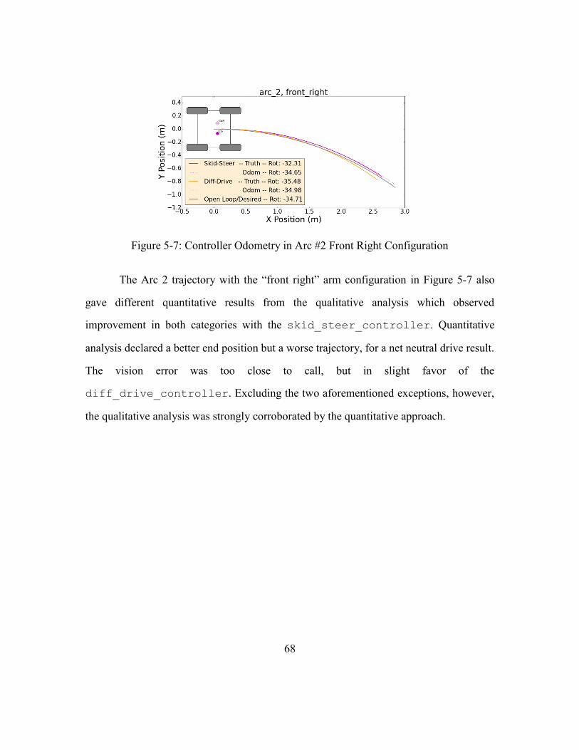
68
Figure 5-7: Controller Odometry in Arc #2 Front Right Configuration
The Arc 2 trajectory with the “front right” arm configuration in Figure 5-7 also
gave different quantitative results from the qualitative analysis which observed
improvement in both categories with the skid_steer_controller. Quantitative
analysis declared a better end position but a worse trajectory, for a net neutral drive result.
The vision error was too close to call, but in slight favor of the
diff_drive_controller. Excluding the two aforementioned exceptions, however,
the qualitative analysis was strongly corroborated by the quantitative approach.

69
Chapter 6: Conclusions and Future Work
The objective of this thesis was to improve the performance of a unique skid-steer
robotic platform with a dynamic center of gravity. To this end, the
skid_steer_controller was developed out of a heuristic model, as an improvement
upon the traditional diff_drive_controller.
6.1. RESEARCH SUMMARY
The VaultBot is a skid-steer mobile manipulator research platform developed by
the NRG for use in hazardous nuclear applications. A relatively large array of actuators
and sensors is linked together using the Robot Operating System (ROS) networking
software from the Open Source Robotics Foundation, and a variety of packages developed
within that framework to support the individual systems. With two output actuators, one
motor for each side of the robot, the mobile base is configured similarly to a traditional
differential-drive system and thus by default utilizes the ROS navigation stack which is
optimized for use with such systems. In practice, however, there are fundamental
differences between differential steering and skid-steering, primarily as a result of the slip
interactions at the wheels. Additionally, these differences are exacerbated and extended by
the VaultBot’s dynamic center-of-gravity (CG) which is a consequence of the onboard
industrial manipulators. A brief series of experiments, the results of which are shown in
Figure 6-1, illuminated the degree to which output behavior varies given the same input
commands but different CG locations.

70
Figure 6-1: Open Loop Trajectories with Varying CG [14]: (A) Legend mapping arm
configuration to color code. (B) “S-curve” trajectory. (C) “Arc” trajectory.
(D) In-place rotation.
In order to develop a better control model based on the CG location, a full kinematic
model of the system was developed. However, this resulted in a system of 6 highly
nonlinear equations with 6 unknowns, to which no closed-form solution could be found. A
cursory look at numeric solvers also did not yield promising results for real-time
implementation, as solutions took an average of 70 seconds. This led to a heuristic
approach in which a grid of 68 different center-of-gravity locations were tested with the
same open loop command, and the resultant trajectories were analyzed for a relationship
between the CG and the apparent center-of-rotation (CoR). This relationship was then
utilized to modify the ROS-based diff_drive_controller package into the

71
skid_steer_controller package. An array of 49 different arm position and open-
loop trajectory configurations were tested with both the new and old controllers in order to
compare results and test for improvement. The results were analyzed both qualitatively and
quantitatively, and both methods came to very similar conclusions.
While the skid_steer_controller was not as drastic of an improvement
as hoped, it did show a net benefit over the diff_drive_controller, particularly in
the in-place rotation behaviors, as well as with the “ready back” and “back left” arm
configurations. Curiously, the diff_drive_controller had consistently better
results with the “front left” arm configuration, for reasons currently unknown. While the
skid_steer_controller is a step in the right direction, there still remains work to
be done.
6.2. FUTURE WORK
In order to further refine the heuristic model, more thorough experimentation could
be performed, with multiple iterations for each CG location and trajectory combination
rather than just one. Also, the model relied on a single in-place rotation trajectory for
development of the CG to CoR relationship; a more robust approach would be to include
multiple trajectory methods. Note that expansion of the experimentation volume is limited
to some extent by physical wear and tear on the robot.
Other approaches also leave room for further work. Working to find a closed-form
solution of the kinematic model could provide a more exact model which could also be
adapted to accommodate additional parameters such as friction coefficients for different
surfaces. This work’s efforts to do so did not yield results after 8 days of computation,
however, so this avenue is not particularly promising. Properly optimized numerical
solvers, on the other hand, may provide an adequate solution. While initial attempts had

72
solve-times well above acceptable limits for real-time implementation, there are a number
of potential approaches to reduce the solve times by one or more orders of magnitude that
have not been fully explored. Whether the reduction is sufficient for real-time operation
remains to be seen.
Finally, while this work focuses on improving the open-loop, odometry side of
skid-steer navigation, there is a large space open for further research into closed-loop
solutions. While the default ROS localization package amcl diverges rapidly in the skid-
steer case, packages such as hector_slam provide highly accurate location tracking in
unknown environments for short periods. Leveraging hector_slam’s accurate laser
scan matching methods into an improved version of amcl could lead to sufficient location
tracking for the VaultBot despite odometry modeling errors, and could be combined with
the methods presented in this work for even better results.
6.3. CONCLUDING REMARKS
The non-linear nature of the slip and friction events inherent to skid-steer
navigation introduces complex behaviors that can be difficult to model. In addition, the
presence of a dynamic center-of-gravity has a significant effect on these behaviors. This
work has clearly shown that the status-quo of ignoring these effects and simply utilizing
the traditional differential steering model is insufficient. While this work has not introduced
a perfect solution which covers all operational cases, it has made significant progress
towards improving the odometry model. This has the potential to not only improve
autonomous navigation performance but also to provide better interaction with a
teleoperator by providing consistent behavior regardless of arm configuration and CG
location.

73
Appendix A: MATLAB Numerical Solver
params.mu_x = 0.9; params.mu_y = 0.9; %Liu et al. values params.K = 13.333; params.f_r = 0.0263; %Liu et al. values params.I = 1/12*118.8437*(0.43^3+0.27^2); params.m = 118.8437; params.r = 0.328/2;
params.d_m = 0.56; params.W_b = 0.52;% VB rough approx. params.g = 9.81; %constant
inputs.F_ext_x = 0; inputs.F_ext_y = 0; inputs.F_ext_z = 0; % external forces (on EEF)
inputs.pe_x = 0; inputs.pe_y = 0; inputs.pe_z = 0; % EEF positions
inputs.x_ddot_M_B = 0; inputs.y_ddot_M_B = 0; % base acceleration
inputs.x_ddot_G_M = 0; inputs.y_ddot_G_M = 0; % COM acceleration
inputs.x_dot_M_B = 0; inputs.y_dot_M_B = 0; %inputs - base velocity
inputs.x_dot_G_M = 0; inputs.y_dot_G_M = 0; %inputs - COM velocity
inputs.x_G_M = 0; inputs.y_G_M = 0; %inputs - COM position
inputs.z_ddot_G_B = 0; %input - COM Z acceleration
inputs.z_G_B = 0.35; %input - COM Z position (VB rough approx.)
inputs.theta_ddot_M = 0; %input - base rot. acceleration
inputs.theta_dot_M = 0; %input - base rot. velocity
function F = Thesis_fsolve(x,params,inputs)
N_fl = x(1);
N_fr = x(2);
N_bl = x(3);
N_br = x(4);
q_dot_l = x(5);
q_dot_r = x(6);
...
parameter/input variable re-assignments
...
%Slip velocities
s_dot_lx = x_dot_M_B - d_m*theta_dot_M/2 - r*q_dot_l;
s_dot_rx = x_dot_M_B + d_m*theta_dot_M/2 - r*q_dot_r;
s_dot_fy = y_dot_M_B + W_b/2*theta_dot_M;
s_dot_by = y_dot_M_B - W_b/2*theta_dot_M;
%Tire friction forces - x
F_x_fl = -mu_x*N_fl*(1-exp(-
K*abs(s_dot_lx)/(1/2*(abs(s_dot_lx+r*q_dot_l)+abs(r*q_dot_l)+abs(abs(s_dot_lx+r*q_dot
_l)-abs(r*q_dot_l))))))*s_dot_lx/sqrt(s_dot_lx^2+s_dot_fy^2);
F_x_fr = -mu_x*N_fr*(1-exp(-
K*abs(s_dot_rx)/(1/2*(abs(s_dot_rx+r*q_dot_r)+abs(r*q_dot_r)+abs(abs(s_dot_rx+r*q_dot
_r)-abs(r*q_dot_r))))))*s_dot_rx/sqrt(s_dot_rx^2+s_dot_fy^2);
F_x_bl = -mu_x*N_bl*(1-exp(-
K*abs(s_dot_lx)/(1/2*(abs(s_dot_lx+r*q_dot_l)+abs(r*q_dot_l)+abs(abs(s_dot_lx+r*q_dot
_l)-abs(r*q_dot_l))))))*s_dot_lx/sqrt(s_dot_lx^2+s_dot_by^2);
F_x_br = -mu_x*N_br*(1-exp(-
K*abs(s_dot_rx)/(1/2*(abs(s_dot_rx+r*q_dot_r)+abs(r*q_dot_r)+abs(abs(s_dot_rx+r*q_dot
_r)-abs(r*q_dot_r))))))*s_dot_rx/sqrt(s_dot_rx^2+s_dot_by^2);
%Tire friction forces - y
F_y_fl = -mu_y*N_fl*(1-exp(-K))*s_dot_fy/sqrt(s_dot_lx^2+s_dot_fy^2);
F_y_fr = -mu_y*N_fr*(1-exp(-K))*s_dot_fy/sqrt(s_dot_rx^2+s_dot_fy^2);
F_y_bl = -mu_y*N_bl*(1-exp(-K))*s_dot_by/sqrt(s_dot_lx^2+s_dot_by^2);

74
F_y_br = -mu_y*N_br*(1-exp(-K))*s_dot_by/sqrt(s_dot_rx^2+s_dot_by^2);
%Rolling resistance
R_fl = f_r*N_fl;
R_fr = f_r*N_fr;
R_bl = f_r*N_bl;
R_br = f_r*N_br;
%CG accelerations
x_ddot_G_B = x_ddot_M_B + x_ddot_G_M - y_G_M*theta_ddot_M-2*y_dot_G_M*theta_dot_M-
x_G_M*theta_dot_M^2;
y_ddot_G_B = y_ddot_M_B + y_ddot_G_M - x_G_M*theta_ddot_M-2*x_dot_G_M*theta_dot_M-
y_G_M*theta_dot_M^2;
% 6 Equations, 6 Unknowns (N_fl,N_fr,N_bl,N_br,q_dot_l,q_dot_r)
F(1) = N_fl + N_fr + N_bl + N_br - m*(g + z_ddot_G_B) + F_ext_z;
F(2) = m*(g + z_ddot_G_B)*(d_m/2 - y_G_M) - pe_z*F_ext_y-F_ext_z*(d_m/2-
pe_y)+m*z_G_B*y_ddot_G_B - d_m*(N_fr + N_br);
F(3) = m*(W_b/2 - x_G_M)*(g + z_ddot_G_B)+m*z_G_B*(x_ddot_G_B) - pe_z*F_ext_x -
F_ext_z*(W_b/2 - pe_x) - W_b*(N_br+N_bl);
F(4) = F_x_fl+F_x_fr+F_x_bl+F_x_br - m*(x_ddot_G_B) - f_r*(m*(g+z_ddot_G_B)-F_ext_z) +
F_ext_x;
F(5) = F_y_fl+F_y_fr+F_y_bl+F_y_br + m*y_ddot_G_B - F_ext_y;
F(6) = (F_y_fl+F_y_fr)*(W_b/2 - x_G_M) - (F_y_bl+F_y_br)*(W_b/2 + x_G_M) + (F_x_fr+F_x_br-
R_fr-R_br)*(d_m/2 + y_G_M)-(F_x_fl+F_x_bl-R_bl-R_fl)*(d_m/2-y_G_M) + F_ext_y*(pe_x -
x_G_M) - F_ext_x*(pe_y - y_G_M) - I*theta_ddot_M;
inputs_gen
params_gen
inputs.x_dot_M_B = 0.3;
inputs.theta_dot_M = 0.1;
fun = @(x) Thesis_fsolve(x,params,inputs);
N_guess = params.m*params.g/4;
q_l_guess = (2*inputs.x_dot_M_B-params.r*inputs.theta_dot_M)/(2*params.r);
q_r_guess = (2*inputs.x_dot_M_B+params.r*inputs.theta_dot_M)/(2*params.r);
x0 = [N_guess,N_guess,N_guess,N_guess,q_l_guess,q_r_guess]
tic
fsolve(fun,x0)
toc

75
Appendix B: Result Trajectories
Figure B-1: Controller Odometry in Arc #1 Back Left Configuration
Figure B-2: Controller Odometry in Arc #1 Back Right Configuration
Figure B-3: Controller Odometry in Arc #1 Front Left Configuration

76
Figure B-4: Controller Odometry in Arc #1 Front Right Configuration
Figure B-5: Controller Odometry in Arc #1 Ready Configuration
Figure B-6: Controller Odometry in Arc #1 Ready Back Configuration

77
Figure B-7: Controller Odometry in Arc #1 Stow Back Configuration
Figure B-8: Controller Odometry in Arc #2 Back Left Configuration
Figure B-9: Controller Odometry in Arc #2 Back Right Configuration

78
Figure B-10: Controller Odometry in Arc #2 Front Left Configuration
Figure B-11: Controller Odometry in Arc #2 Front Right Configuration
Figure B-12: Controller Odometry in Arc #2 Ready Configuration
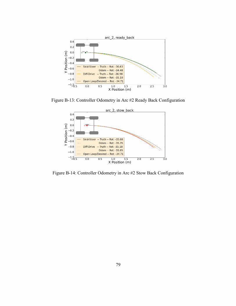
79
Figure B-13: Controller Odometry in Arc #2 Ready Back Configuration
Figure B-14: Controller Odometry in Arc #2 Stow Back Configuration

80
Figure B-15: Controller Odometry in Arc #3 Back Left Configuration
Figure B-16: Controller Odometry in Arc #3 Back Right Configuration

81
Figure B-17: Controller Odometry in Arc #3 Front Left Configuration
Figure B-18: Controller Odometry in Arc #3 Front Right Configuration

82
Figure B-19: Controller Odometry in Arc #3 Ready Configuration
Figure B-20: Controller Odometry in Arc #3 Ready Back Configuration
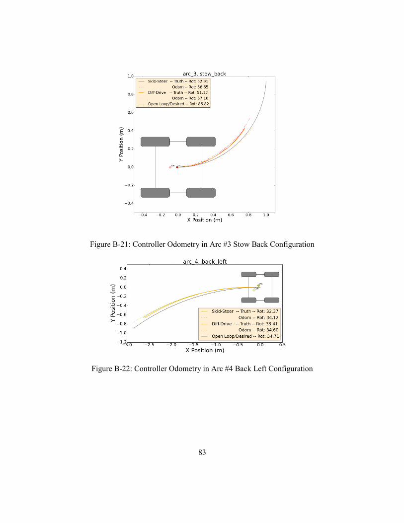
83
Figure B-21: Controller Odometry in Arc #3 Stow Back Configuration
Figure B-22: Controller Odometry in Arc #4 Back Left Configuration

84
Figure B-23: Controller Odometry in Arc #4 Back Right Configuration
Figure B-24: Controller Odometry in Arc #4 Front Left Configuration
Figure B-25: Controller Odometry in Arc #4 Front Right Configuration
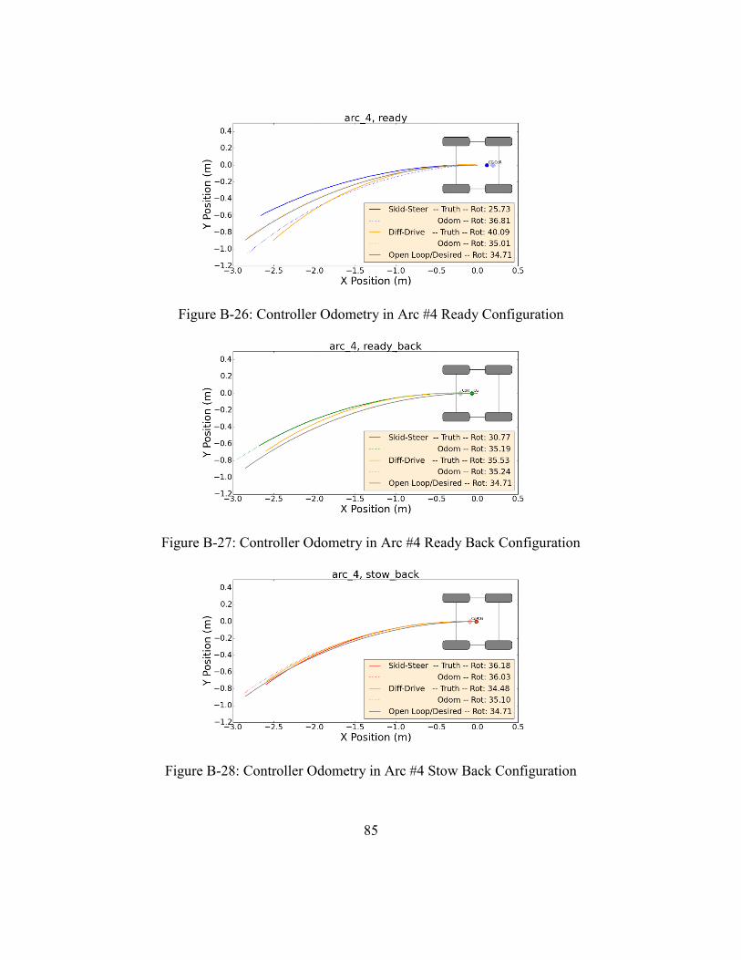
85
Figure B-26: Controller Odometry in Arc #4 Ready Configuration
Figure B-27: Controller Odometry in Arc #4 Ready Back Configuration
Figure B-28: Controller Odometry in Arc #4 Stow Back Configuration
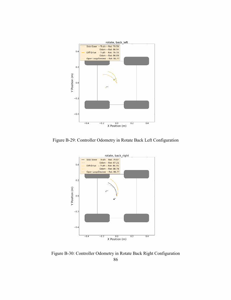
86
Figure B-29: Controller Odometry in Rotate Back Left Configuration
Figure B-30: Controller Odometry in Rotate Back Right Configuration

87
Figure B-31: Controller Odometry in Rotate Front Left Configuration
Figure B-32: Controller Odometry in Rotate Front Right Configuration

88
Figure B-33: Controller Odometry in Rotate Ready Configuration
Figure B-34: Controller Odometry in Rotate Ready Back Configuration

89
Figure B-35: Controller Odometry in Rotate Stow Back Configuration
Figure B-36: Controller Odometry in S-curve Back Left Configuration

90
Figure B-37: Controller Odometry in S-curve Back Right Configuration
Figure B-38: Controller Odometry in S-curve Front Left Configuration

91
Figure B-39: Controller Odometry in S-curve Front Right Configuration
Figure B-40: Controller Odometry in S-curve Ready Configuration
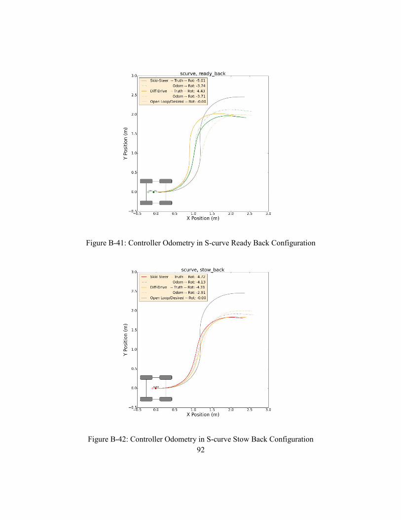
92
Figure B-41: Controller Odometry in S-curve Ready Back Configuration
Figure B-42: Controller Odometry in S-curve Stow Back Configuration

93
References
[1] K. Nagatani, S. Kiribayashi, Y. Okada, K. Otake, K. Yoshida, S. Tadokoro, T.
Nishimura, T. Yoshida, E. Koyanagi, M. Fukushima, and S. Kawatsuma,
“Emergency Response to the Nuclear Accident at the Fukushima Daiichi Nuclear
Power Plants using Mobile Rescue Robots,” J. F. Robot., vol. 30, no. 1, pp. 44–63,
2013.
[2] J. Franco and T. Reynolds, “Carlsbad Town Hall Meeting, April 17, 2014,” US
Department of Energy; Waste Isolation Pilot Plant, 2014.
[3] R. Bogue, “Robots in the nuclear industry: a review of technologies and
applications,” Ind. Robot An Int. J., vol. 38, no. 2, pp. 113–118, Mar. 2011.
[4] A. Griffiths, A. Dikarev, P. R. Green, B. Lennox, X. Poteau, and S. Watson,
“AVEXIS—Aqua Vehicle Explorer for In-Situ Sensing,” IEEE Robot. Autom.
Lett., vol. 1, no. 1, 2016.
[5] K. Nagatani, S. Kiribayashi, Y. Okada, S. Tadokoro, T. Nishimura, T. Yoshida, E.
Koyanagi, and Y. Hada, “Redesign of rescue mobile robot Quince,” in Safety,
Security, and Rescue Robotics (SSRR), 2011 IEEE International Symposium on,
2011, pp. 13–18.
[6] H. Li, B. Li, and W. Xu, “Development of a remote-controlled mobile robot with
binocular vision for environment monitoring,” in 2015 IEEE International
Conference on Information and Automation, 2015, pp. 737–742.
[7] Y. Huang, W. Wang, and D. Wu, “Development and Optimum Design of a Mobile
Manipulator for CBRN Sampling,” in Proceedings of the 11th World Congress on
Intelliegent Control and Automation, 2014, pp. 525–530.
[8] P. Besset, “Inverse kinematics for a redundant hydraulic robotic manipulator used
for nuclear decommissioning,” in 2014 UKACC International Conference on
Control, 2013, no. September.
[9] S. Notheis, P. Kern, M. Mende, B. Hein, H. Wörn, and S. Gentes, “Towards an
Autonomous Manipulator System for Decontamination and Release
Measurement,” pp. 263–268, 2012.
[10] T. Wang, Y. Wu, J. Liang, C. Han, J. Chen, and Q. Zhao, “Analysis and
experimental kinematics of a skid-steering wheeled robot based on a laser scanner
sensor.,” Sensors (Basel)., vol. 15, no. 5, pp. 9681–702, 2015.
[11] M. Quigley, K. Conley, B. Gerkey, J. FAust, T. Foote, J. Leibs, E. Berger, R.
Wheeler, and A. Mg, “ROS: an open-source Robot Operating System,” Icra, vol.
3, no. Figure 1, p. 5, 2009.
[12] B. Gerkey, “AMCL.” [Online]. Available: http://wiki.ros.org/amcl. [Accessed: 13-

94
Nov-2016].
[13] E. Marder-Eppstein, “navigation.” [Online]. Available:
http://wiki.ros.org/navigation. [Accessed: 13-Nov-2016].
[14] B. Ebersole and M. Pryor, “Intelligent navigation of a skid steer dual-arm
manipulator with dynamic center of gravity,” in D&RS 2016 (Decommissioning
and Remote Systems), 2016, pp. 179–184.
[15] R. C. Goertz, “Master-slave Manipulator,” Argonne National Laboratory, 1949.
[16] T. Moore, “Robots for nuclear power plants,” pp. 31–38, 1985.
[17] L. Briones, P. Bustamante, and M. a. Serna, “Wall-climbing robot for inspection in
nuclear power plants,” in Proceedings of the 1994 IEEE International Conference
on Robotics and Automation, 1994, pp. 1409–1414.
[18] N. Ishikawa and K. Suzuki, “Development of a human and robot collaborative
system for inspecting patrol of nuclear power plants,” in Robot and Human
Communication, 1997. RO-MAN ’97. Proceedings., 6th IEEE International
Workshop on, 1997, pp. 118–123.
[19] Y. Iwano, K. Osuka, and H. Amano, “Proposal of a rescue robot system in nuclear-
power plants-rescue activity via small vehicle robots,” in Proceedings - 2004 IEEE
International Conference on Robotics and Biomimetics, IEEE ROBIO 2004, 2004,
pp. 227–232.
[20] C. Ducros, G. Hauser, N. Mahjoubi, P. Girones, L. Boisset, A. Sorin, E. Jonquet, J.
M. Falciola, and A. Benhamou, “RICA: A Tracked Robot for Sampling and
Radiological Characterization in the Nuclear Field,” J. F. Robot., May 2016.
[21] G. Jiang, R. Voyles, K. Sebesta, and H. Greiner, “Mock-up of the exhaust shaft
inspection by dexterous hexrotor at the DOE WIPP site,” in 2015 IEEE
International Symposium on Safety, Security, and Rescue Robotics (SSRR), 2015,
pp. 1–2.
[22] D. Kanaan, S. Dogny, and T. Varet, “Robot for investigations and assessments of
nuclear areas,” in 2015 4th International Conference on Advancements in Nuclear
Instrumentation Measurement Methods and their Applications (ANIMMA), 2015,
pp. 1–4.
[23] E. Trulls, A. Corominas Murtra, J. Pérez-Ibarz, G. Ferrer, D. Vasquez, J. M.
Mirats-Tur, and A. Sanfeliu, “Autonomous navigation for mobile service robots in
urban pedestrian environments,” J. F. Robot., vol. 28, no. 3, pp. 329–354, May
2011.
[24] A. Stentz, H. Herman, A. Kelly, E. Meyhofer, G. C. Haynes, D. Stager, B. Zajac,
J. A. Bagnell, J. Brindza, C. Dellin, M. George, J. Gonzalez-Mora, S. Hyde, M.
Jones, M. Laverne, M. Likhachev, L. Lister, M. Powers, O. Ramos, J. Ray, D.

95
Rice, J. Scheifflee, R. Sidki, S. Srinivasa, K. Strabala, J.-P. Tardif, J.-S. Valois, J.
M. Vande Weghe, M. Wagner, and C. Wellington, “CHIMP, the CMU Highly
Intelligent Mobile Platform,” J. F. Robot., vol. 32, no. 2, pp. 209–228, Mar. 2015.
[25] P. Hebert, M. Bajracharya, J. Ma, N. Hudson, A. Aydemir, J. Reid, C. Bergh, J.
Borders, M. Frost, M. Hagman, J. Leichty, P. Backes, B. Kennedy, P. Karplus, B.
Satzinger, K. Byl, K. Shankar, and J. Burdick, “Mobile Manipulation and Mobility
as Manipulation-Design and Algorithms of RoboSimian,” J. F. Robot., vol. 32, no.
2, pp. 255–274, Mar. 2015.
[26] P. Ben-Tzvi, “Experimental validation and field performance metrics of a hybrid
mobile robot mechanism,” J. F. Robot., vol. 27, no. 3, p. n/a-n/a, 2010.
[27] L. He, “Tip-over Avoidance Algorithm for Modular Mobile Manipulator *,” in
First International Conference on Innovative Engineering Systems, 2012, pp. 115–
120.
[28] S. Ide, T. Takubo, K. Ohara, Y. Mae, and T. Arai, “Real-time trajectory planning
for mobile manipulator using model predictive control with constraints,” in 2011
8th International Conference on Ubiquitous Robots and Ambient Intelligence
(URAI), 2011, pp. 244–249.
[29] Y. Liu and G. Liu, “Modeling of tracked mobile manipulators with consideration
of track-terrain and vehicle-manipulator interactions,” Rob. Auton. Syst., vol. 57,
no. 11, pp. 1065–1074, 2009.
[30] L. Caracciolo, A. de Luca, and S. Iannitti, “Trajectory tracking control of a four-
wheel differentially driven mobile robot,” in Proceedings 1999 IEEE International
Conference on Robotics and Automation (Cat. No.99CH36288C), 1999, vol. 4, no.
May, pp. 2632–2638.
[31] K. Kozlowski and D. Pazderski, “Modeling and control of a 4-wheel skid-steering
mobile robot,” Int. J. Appl. Math. Comput. Sci., vol. 14, no. 4, pp. 477–496, 2004.
[32] J. Pentzer, S. Brennan, and K. Reichard, “Model-based Prediction of Skid-steer
Robot Kinematics Using Online Estimation of Track Instantaneous Centers of
Rotation,” J. F. Robot., vol. 31, no. 3, pp. 455–476, May 2014.
[33] A. Mandow, J. L. Martínez, J. Morales, J. L. Blanco, A. García-Cerezo, and J.
González, “Experimental kinematics for wheeled skid-steer mobile robots,” in
IEEE International Conference on Intelligent Robots and Systems, 2007, pp.
1222–1227.
[34] “Motion Capture Systems | VICON.” [Online]. Available:
https://www.vicon.com/. [Accessed: 09-Nov-2016].
[35] “Fit Data with a Neural Network.” [Online]. Available:
http://www.mathworks.com/help/nnet/gs/fit-data-with-a-neural-network.html.

96
[Accessed: 09-Nov-2016].
[36] S. Kohlbrecher, O. Von Stryk, J. Meyer, and U. Klingauf, “A Flexible and
Scalable SLAM System with Full 3D Motion Estimation,” IEEE Int. Symp. Safety,
Secur. Rescue Robot., 2011.
[37] P. Corke, “Denavit-Hartenberg notation for common robots,” 2014. [Online].
Available: http://petercorke.com/doc/rtb_dh.pdf. [Accessed: 09-Nov-2016].
[38] “Actual center of mass for robot.” [Online]. Available: http://www.universal-
robots.com/how-tos-and-faqs/faq/ur-faq/actual-center-of-mass-for-robot-17264/.
[Accessed: 09-Nov-2016].
[39] A. C. Cameron, “Excel 2007: Multiple Regression,” 2009. [Online]. Available:
http://cameron.econ.ucdavis.edu/excel/ex61multipleregression.html. [Accessed:
09-Nov-2016].