Copyright Agrawal, 2007 ELEC6270 Fall 07, Lecture 8 1 ELEC 5270/6270 Fall 2007 Low-Power Design of...

Copyright Agrawal, 2007Copyright Agrawal, 2007 ELEC6270 Fall 07, Lecture 8ELEC6270 Fall 07, Lecture 8 11

ELEC 5270/6270 Fall 2007ELEC 5270/6270 Fall 2007Low-Power Design of Electronic CircuitsLow-Power Design of Electronic Circuits

Linear Programming – A Mathematical Linear Programming – A Mathematical Optimization TechniqueOptimization Technique

Vishwani D. AgrawalVishwani D. AgrawalJames J. Danaher ProfessorJames J. Danaher Professor

Dept. of Electrical and Computer EngineeringDept. of Electrical and Computer EngineeringAuburn University, Auburn, AL 36849Auburn University, Auburn, AL 36849

[email protected]://www.eng.auburn.edu/~vagrawal/COURSE/E6270_Fall07/course.html


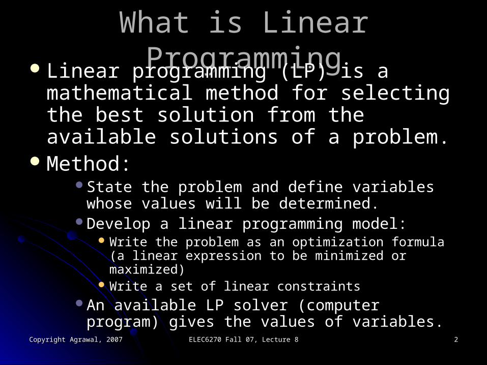
What is Linear ProgrammingWhat is Linear ProgrammingLinear programming (LP) is a Linear programming (LP) is a

mathematical method for selecting the mathematical method for selecting the best solution from the available solutions best solution from the available solutions of a problem.of a problem.

Method:Method:State the problem and define variables whose State the problem and define variables whose

values will be determined.values will be determined.Develop a linear programming model:Develop a linear programming model:

Write the problem as an optimization formula (a linear Write the problem as an optimization formula (a linear expression to be minimized or maximized)expression to be minimized or maximized)

Write a set of linear constraintsWrite a set of linear constraintsAn available LP solver (computer program) gives An available LP solver (computer program) gives

the values of variables.the values of variables.


Types of LPsTypes of LPs

LP – all variables are real.LP – all variables are real. ILP – all variables are integers.ILP – all variables are integers.MILP – some variables are integers, MILP – some variables are integers,

others are real.others are real.A reference:A reference:

S. I. Gass, An Illustrated Guide to Linear S. I. Gass, An Illustrated Guide to Linear Programming, New York: Dover, 1990.Programming, New York: Dover, 1990.


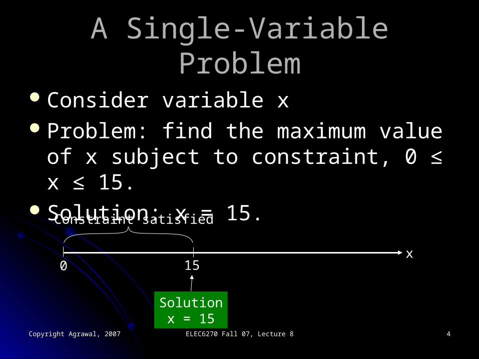
A Single-Variable ProblemA Single-Variable Problem

Consider variable xConsider variable xProblem: find the maximum value of x Problem: find the maximum value of x

subject to constraint, 0 ≤ x ≤ 15.subject to constraint, 0 ≤ x ≤ 15.Solution: x = 15.Solution: x = 15.

0 15

Constraint satisfied

x

Solution x = 15


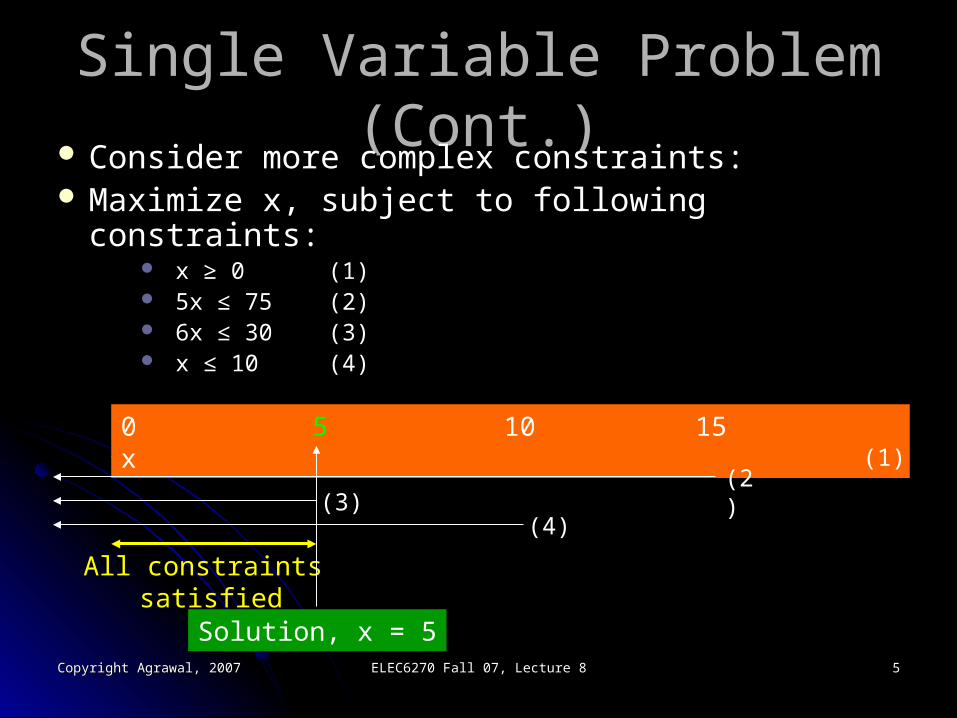
Single Variable Problem (Cont.)Single Variable Problem (Cont.) Consider more complex constraints:Consider more complex constraints: Maximize x, subject to following constraints:Maximize x, subject to following constraints:

x ≥ 0x ≥ 0 (1)(1) 5x ≤ 755x ≤ 75 (2)(2) 6x ≤ 306x ≤ 30 (3)(3) x ≤ 10x ≤ 10 (4)(4)

0 5 10 15x (1)

(2)(3)

(4)

All constraints satisfied

Solution, x = 5


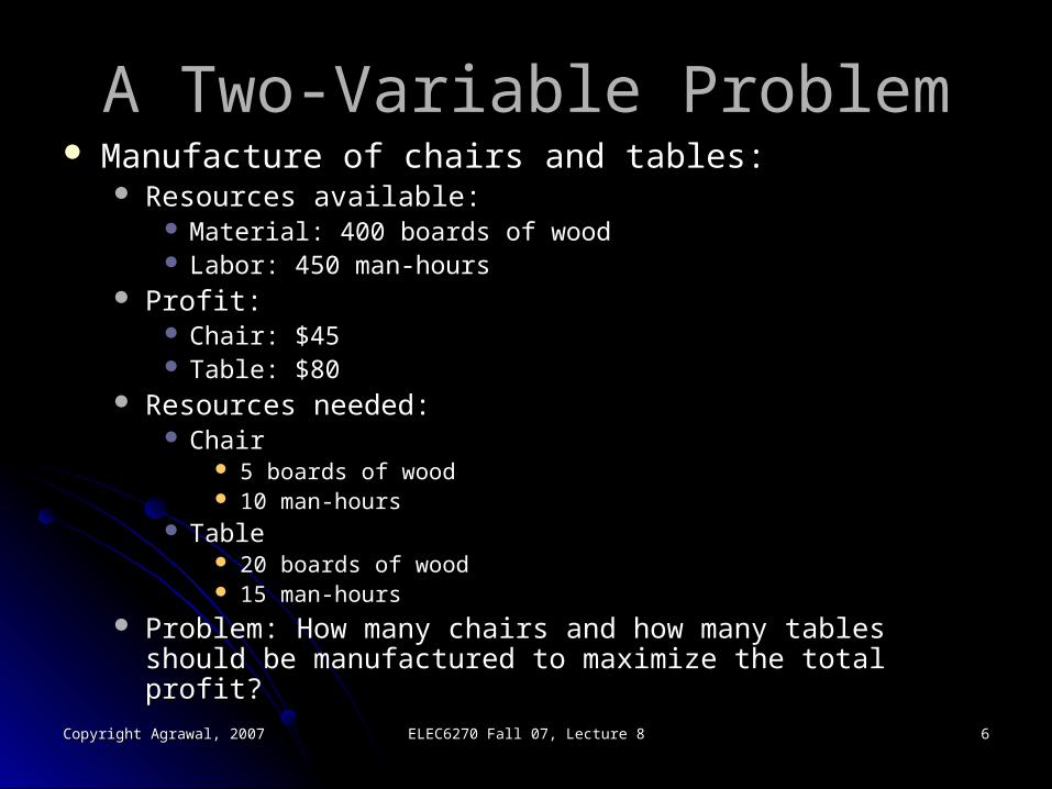
A Two-Variable ProblemA Two-Variable Problem Manufacture of chairs and tables:Manufacture of chairs and tables:

Resources available:Resources available: Material: 400 boards of woodMaterial: 400 boards of wood Labor: 450 man-hoursLabor: 450 man-hours

Profit:Profit: Chair: $45Chair: $45 Table: $80Table: $80

Resources needed:Resources needed: ChairChair

5 boards of wood5 boards of wood 10 man-hours10 man-hours

TableTable 20 boards of wood20 boards of wood 15 man-hours15 man-hours

Problem: How many chairs and how many tables should be Problem: How many chairs and how many tables should be manufactured to maximize the total profit?manufactured to maximize the total profit?


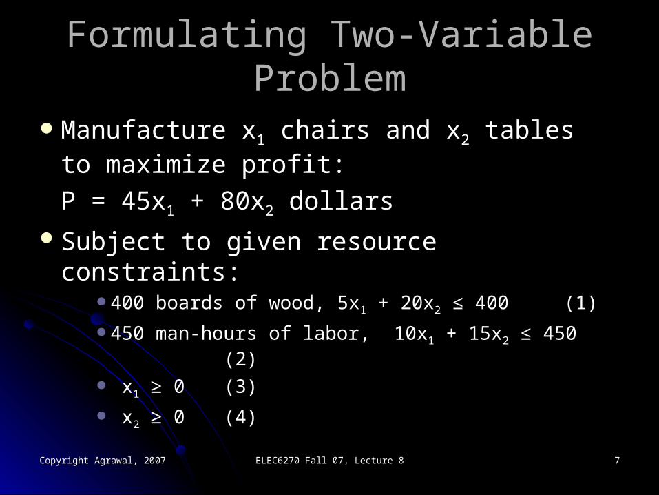
Formulating Two-Variable ProblemFormulating Two-Variable Problem

Manufacture xManufacture x11 chairs and x chairs and x22 tables to tables to

maximize profit:maximize profit:

P = 45xP = 45x11 + 80x + 80x22 dollars dollarsSubject to given resource constraints:Subject to given resource constraints:

400 boards of wood,400 boards of wood, 5x5x11 + 20x + 20x22 ≤ 400 ≤ 400 (1)(1)

450 man-hours of labor,450 man-hours of labor, 10x10x11 + 15x + 15x22 ≤ 450 ≤ 450 (2)(2)

xx11 ≥ 0 ≥ 0 (3)(3)

xx22 ≥ 0 ≥ 0 (4)(4)


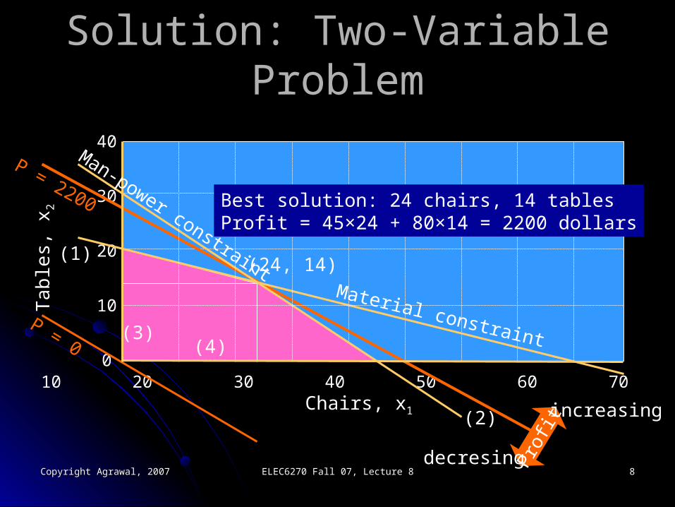
Solution: Two-Variable ProblemSolution: Two-Variable Problem

Chairs, x1

Tab

les,

x2

(1)

(2)

0 10 20 30 40 50 60 70 80 90

40

30

20

10

0

(24, 14)

Profi

t increasing

decresing

P = 2200

P = 0

Best solution: 24 chairs, 14 tablesProfit = 45×24 + 80×14 = 2200 dollars

(3)(4)

Material constraint

Man-power constraint


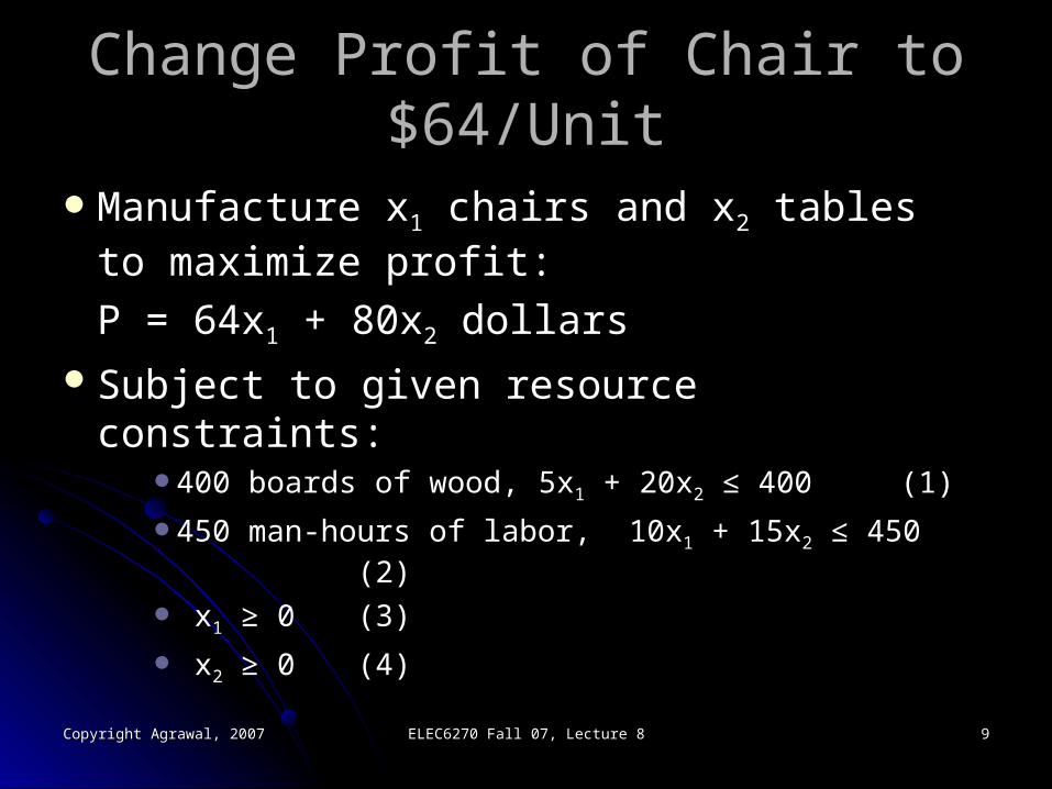
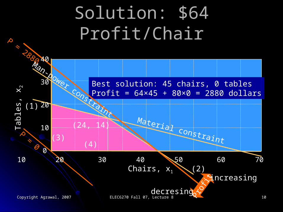
Change Profit of Chair to $64/UnitChange Profit of Chair to $64/Unit

Manufacture xManufacture x11 chairs and x chairs and x22 tables to tables to

maximize profit:maximize profit:

P = 64xP = 64x11 + 80x + 80x22 dollars dollarsSubject to given resource constraints:Subject to given resource constraints:

400 boards of wood,400 boards of wood, 5x5x11 + 20x + 20x22 ≤ 400 ≤ 400 (1)(1)

450 man-hours of labor,450 man-hours of labor, 10x10x11 + 15x + 15x22 ≤ 450 ≤ 450 (2)(2)

xx11 ≥ 0 ≥ 0 (3)(3)

xx22 ≥ 0 ≥ 0 (4)(4)


Solution: $64 Profit/ChairSolution: $64 Profit/Chair

Chairs, x1

Tab

les,

x2

(1)

(2)

Profi

t increasing

decresing

P = 2880

P = 0

Best solution: 45 chairs, 0 tablesProfit = 64×45 + 80×0 = 2880 dollars

0 10 20 30 40 50 60 70 80 90

(24, 14)

40

30

20

10

0

(3)(4)

Material constraint

Man-power constraint


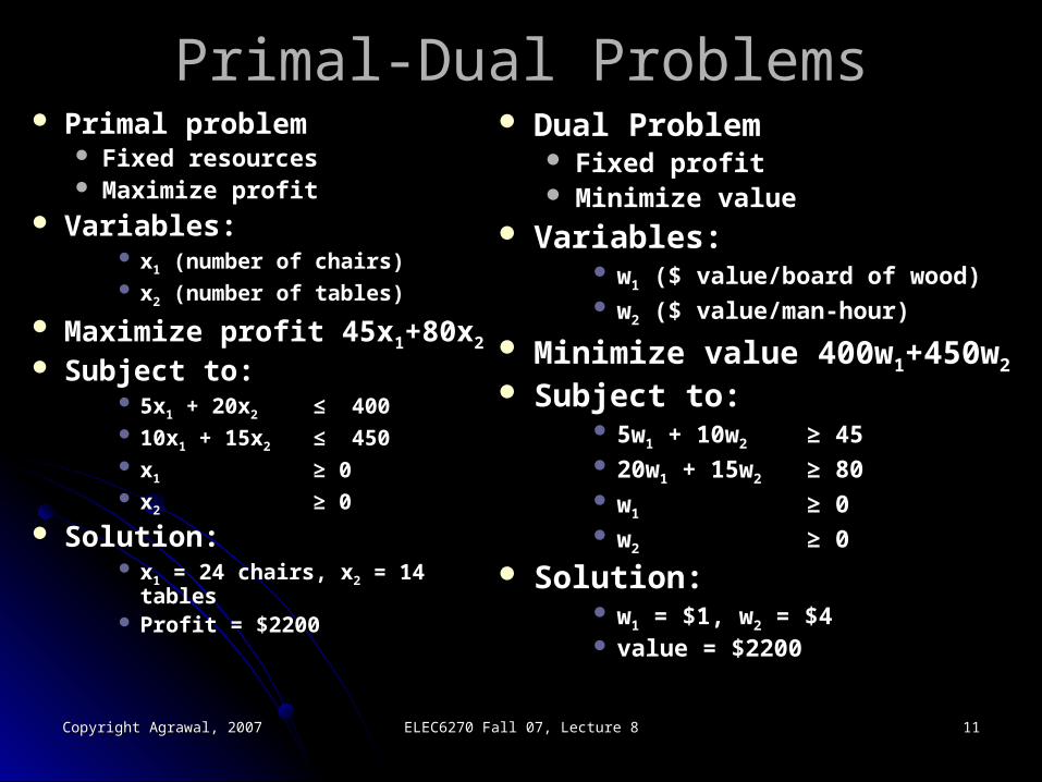
Primal-Dual ProblemsPrimal-Dual Problems Primal problemPrimal problem

Fixed resourcesFixed resources Maximize profitMaximize profit

Variables:Variables: xx11 (number of chairs) (number of chairs) xx22 (number of tables) (number of tables)

Maximize profit 45xMaximize profit 45x11+80x+80x22

Subject to:Subject to: 5x5x11 + 20x + 20x22 ≤ 400≤ 400 10x10x11 + 15x + 15x22 ≤≤ 450 450 xx11 ≥ 0≥ 0 xx22 ≥ 0≥ 0

Solution:Solution: xx11 = 24 chairs, x = 24 chairs, x22 = 14 tables = 14 tables Profit = $2200Profit = $2200

Dual ProblemDual Problem Fixed profitFixed profit Minimize valueMinimize value

Variables:Variables: ww11 ($ value/board of wood) ($ value/board of wood) ww22 ($ value/man-hour) ($ value/man-hour)

Minimize value 400wMinimize value 400w11+450w+450w22

Subject to:Subject to: 5w5w11 + 10w + 10w22 ≥ 45≥ 45 20w20w11 + 15w + 15w2 2 ≥ 80≥ 80 ww11 ≥ 0≥ 0 ww22 ≥ 0≥ 0

Solution:Solution: ww11 = $1, w = $1, w22 = $4 = $4 value = $2200value = $2200


The Duality TheoremThe Duality Theorem

If the primal has a finite optimal solution, If the primal has a finite optimal solution, so does the dual, and the optimum values so does the dual, and the optimum values of the objective functions are equal.of the objective functions are equal.


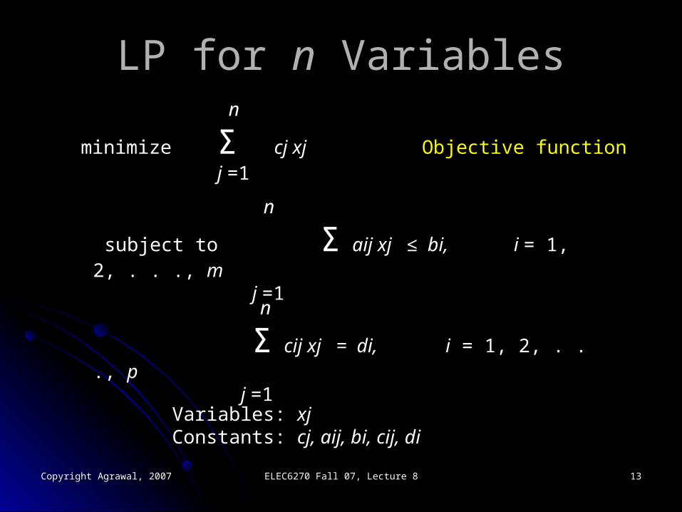
LP for LP for nn Variables Variables n

minimize Σ cj xj Objective functionj =1

n

subject to Σ aij xj ≤ bi, i = 1, 2, . . ., m j =1

n

Σ cij xj = di, i = 1, 2, . . ., p j =1

Variables: xjConstants: cj, aij, bi, cij, di


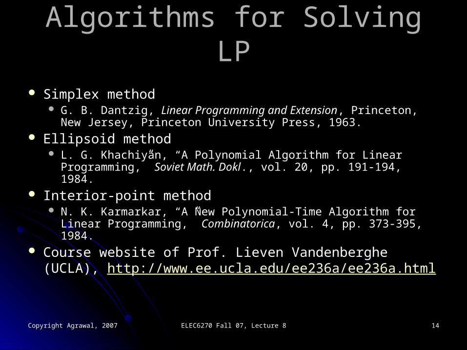
Algorithms for Solving LPAlgorithms for Solving LP

Simplex methodSimplex method G. B. Dantzig, G. B. Dantzig, Linear Programming and ExtensionLinear Programming and Extension, Princeton, , Princeton,

New Jersey, Princeton University Press, 1963.New Jersey, Princeton University Press, 1963. Ellipsoid methodEllipsoid method

L. G. Khachiyan, “A Polynomial Algorithm for Linear L. G. Khachiyan, “A Polynomial Algorithm for Linear Programming,” Programming,” Soviet Math. DoklSoviet Math. Dokl., vol. 20, pp. 191-194, 1984.., vol. 20, pp. 191-194, 1984.

Interior-point methodInterior-point method N. K. Karmarkar, “A New Polynomial-Time Algorithm for Linear N. K. Karmarkar, “A New Polynomial-Time Algorithm for Linear

Programming,” Programming,” CombinatoricaCombinatorica, vol. 4, pp. 373-395, 1984., vol. 4, pp. 373-395, 1984. Course website of Prof. Lieven Vandenberghe (UCLA), Course website of Prof. Lieven Vandenberghe (UCLA),

http://www.ee.ucla.edu/ee236a/ee236a.htmlhttp://www.ee.ucla.edu/ee236a/ee236a.html


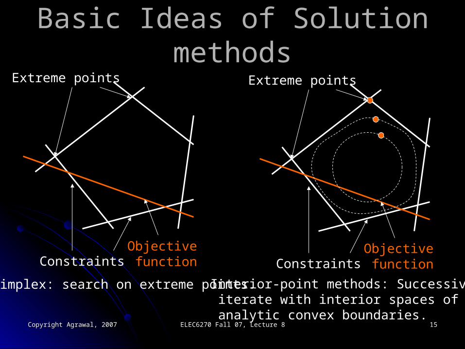
Basic Ideas of Solution methodsBasic Ideas of Solution methods

Constraints

Extreme points

Objective function Constraints

Extreme points

Objective function

Simplex: search on extreme points.Interior-point methods: Successively iterate with interior spaces of analytic convex boundaries.


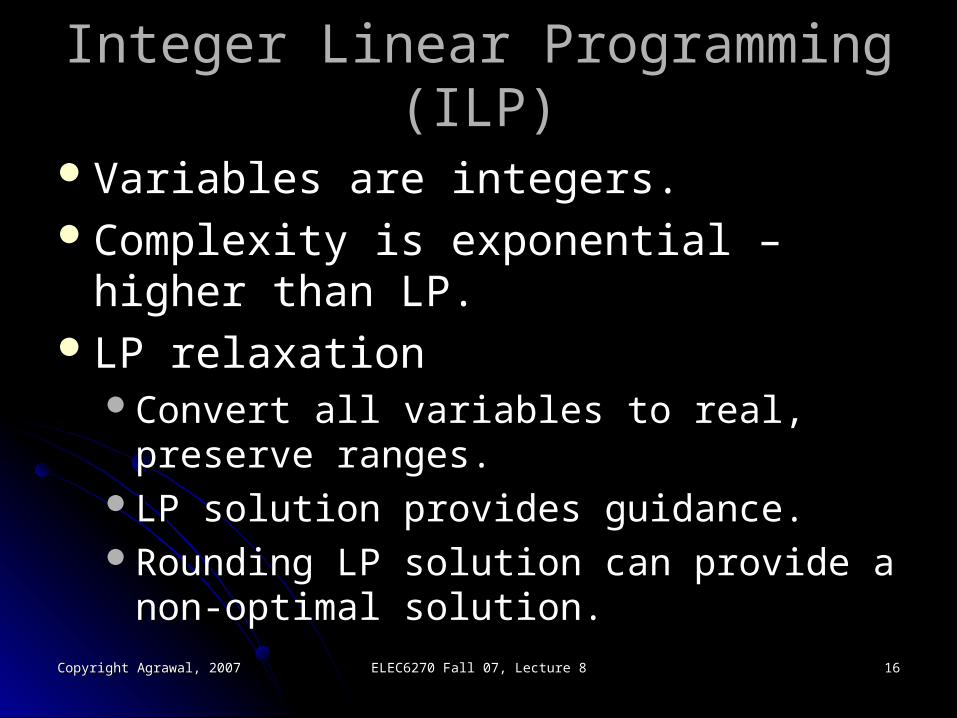
Integer Linear Programming (ILP)Integer Linear Programming (ILP)

Variables are integers.Variables are integers.Complexity is exponential – higher than LP.Complexity is exponential – higher than LP.LP relaxationLP relaxation

Convert all variables to real, preserve ranges.Convert all variables to real, preserve ranges.LP solution provides guidance.LP solution provides guidance.Rounding LP solution can provide a non-Rounding LP solution can provide a non-

optimal solution.optimal solution.


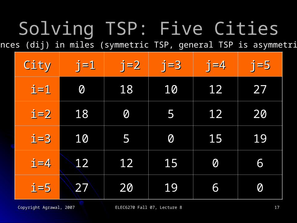
Solving TSP: Five CitiesSolving TSP: Five CitiesDistances (dij) in miles (symmetric TSP, general TSP is asymmetric)

CityCity j=1j=1 j=2j=2 j=3j=3 j=4j=4 j=5j=5

i=1i=1 00 1818 1010 1212 2727

i=2i=2 1818 00 55 1212 2020

i=3i=3 1010 55 00 1515 1919

i=4i=4 1212 1212 1515 00 66

i=5i=5 2727 2020 1919 66 00


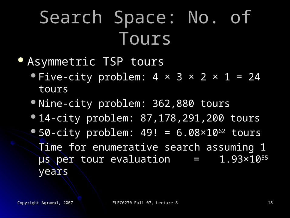
Search Space: No. of ToursSearch Space: No. of Tours

Asymmetric TSP toursAsymmetric TSP toursFive-city problem: 4 Five-city problem: 4 × 3 × 2 × 1 = 24 tours× 3 × 2 × 1 = 24 toursNine-city problem: 362,880 toursNine-city problem: 362,880 tours14-city problem: 87,178,291,200 tours14-city problem: 87,178,291,200 tours50-city problem: 49! = 6.08×1050-city problem: 49! = 6.08×1062 tours tours

Time for enumerative search assuming 1 Time for enumerative search assuming 1 μμs s per tour evaluationper tour evaluation == 1.93×101.93×1055 years years


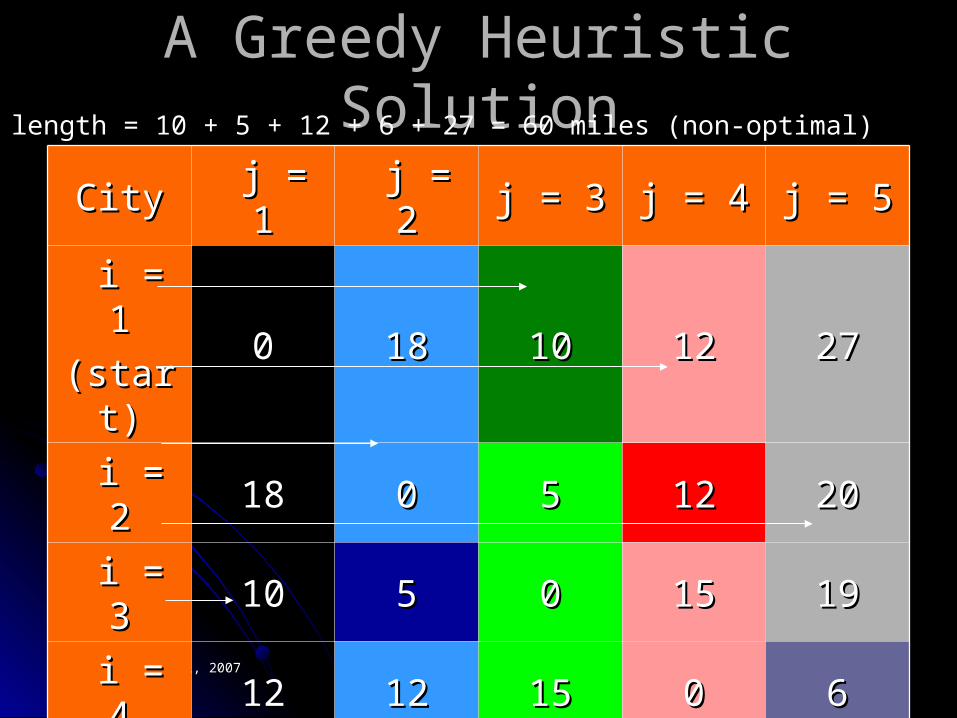
A Greedy Heuristic SolutionA Greedy Heuristic Solution

CityCity j = 1j = 1 j = 2j = 2 j = 3j = 3 j = 4j = 4 j = 5j = 5

i = 1i = 1

(start)(start)00 1818 1010 1212 2727

i = 2i = 2 1818 00 55 1212 2020

i = 3i = 3 1010 55 00 1515 1919

i = 4i = 4 1212 1212 1515 00 66

i = 5i = 5 2727 2020 1919 66 00

Tour length = 10 + 5 + 12 + 6 + 27 = 60 miles (non-optimal)


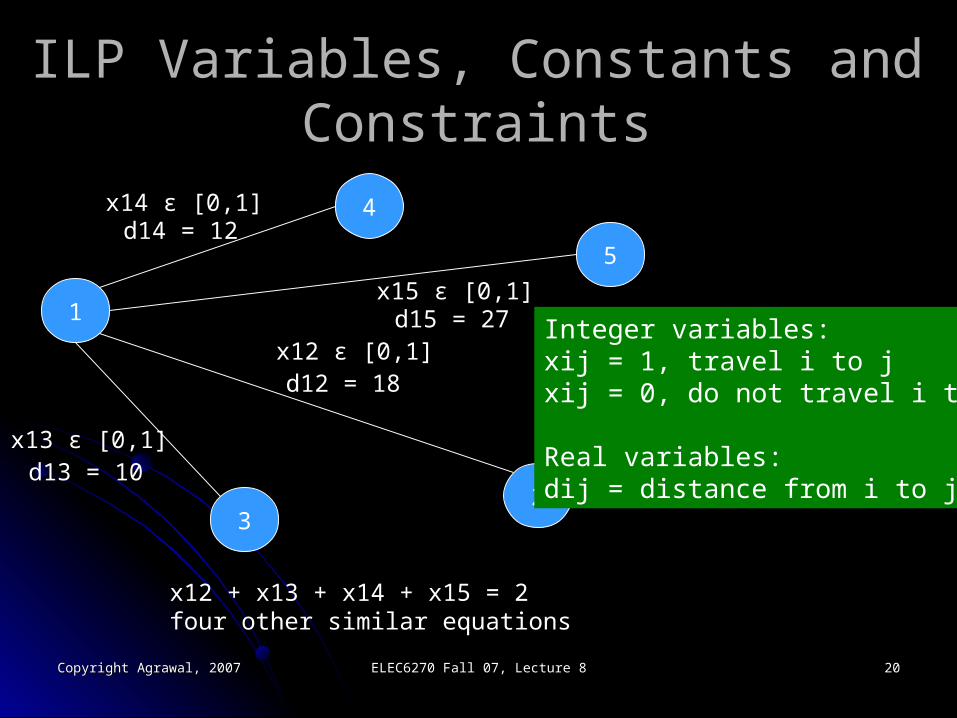
ILP Variables, Constants and ILP Variables, Constants and ConstraintsConstraints

1

32

5

4 d14 = 12

d15 = 27

d12 = 18

d13 = 10

x14 ε [0,1]

x15 ε [0,1]

x12 ε [0,1]

x13 ε [0,1]

x12 + x13 + x14 + x15 = 2 four other similar equations

Integer variables:xij = 1, travel i to jxij = 0, do not travel i to j

Real variables:dij = distance from i to j


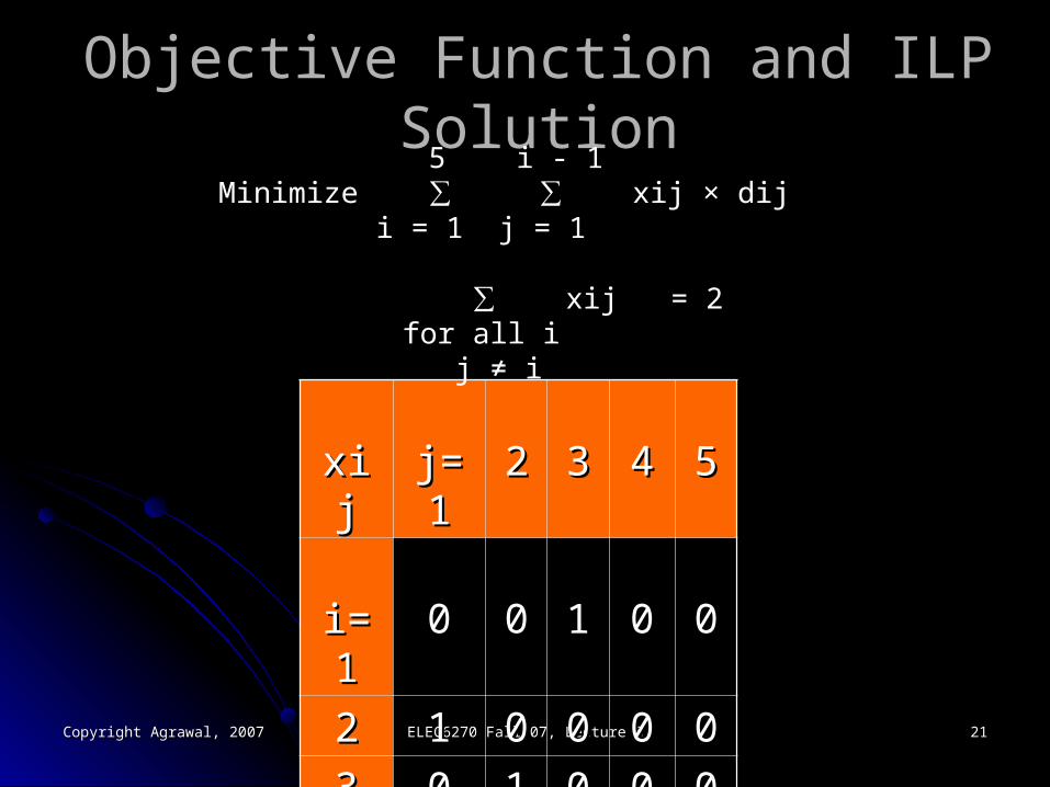
Objective Function and ILP SolutionObjective Function and ILP Solution 5 i - 1

Minimize ∑ ∑ xij × dij i = 1 j = 1

xijxij j=1j=1 22 33 44 55

i=1i=1 00 00 11 00 00

22 11 00 00 00 00

33 00 11 00 00 00

44 00 00 00 00 11

55 00 00 00 11 00

∑ xij = 2 for all i j ≠ i


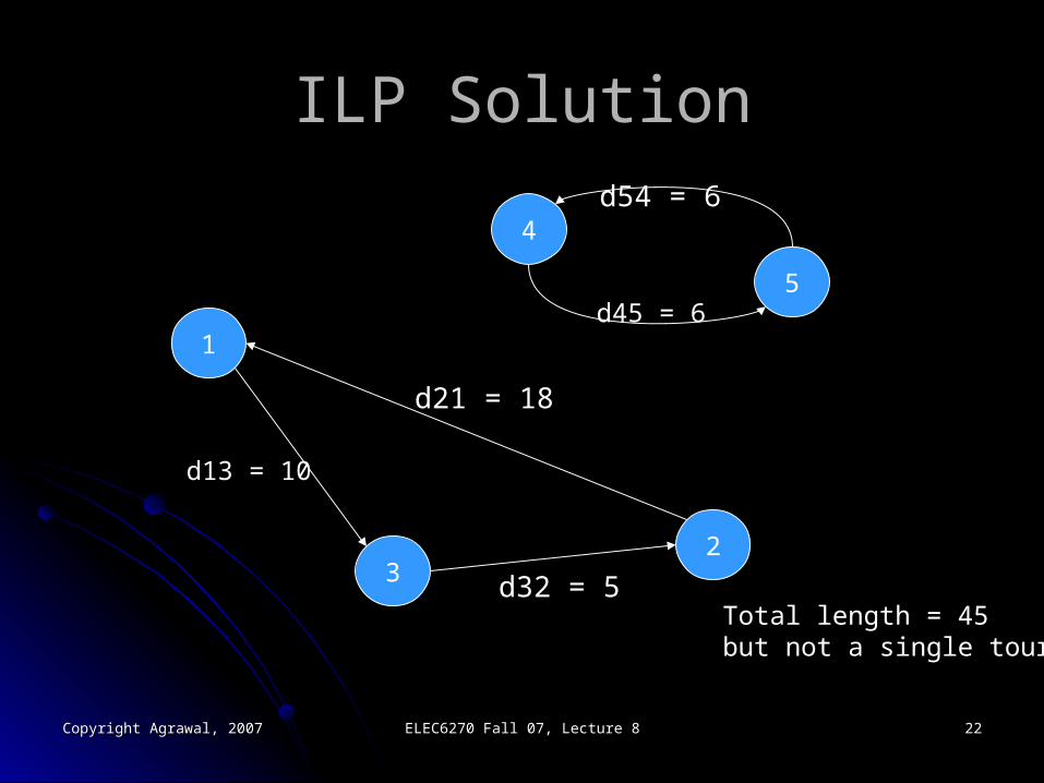
ILP SolutionILP Solution

1

32

5

4

d13 = 10

d45 = 6

Total length = 45 but not a single tour

d54 = 6

d21 = 18

d32 = 5


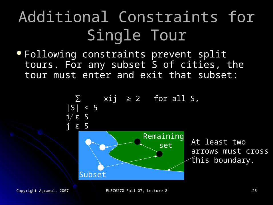
Additional Constraints for Single TourAdditional Constraints for Single Tour

Following constraints prevent split tours. Following constraints prevent split tours. For any subset S of cities, the tour must For any subset S of cities, the tour must enter and exit that subset:enter and exit that subset:

∑ xij ≥ 2 for all S, |S| < 5i ε S j ε S

Subset

Remaining set At least two

arrows must crossthis boundary.


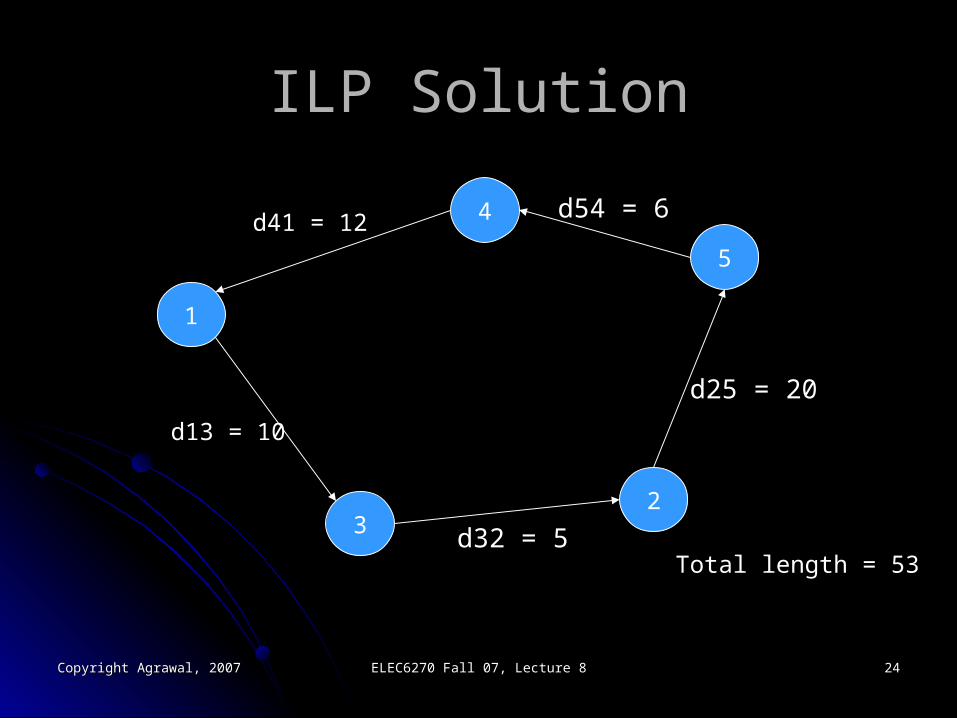
ILP SolutionILP Solution

1

32

5

4

d13 = 10

d41 = 12

Total length = 53

d54 = 6

d25 = 20

d32 = 5


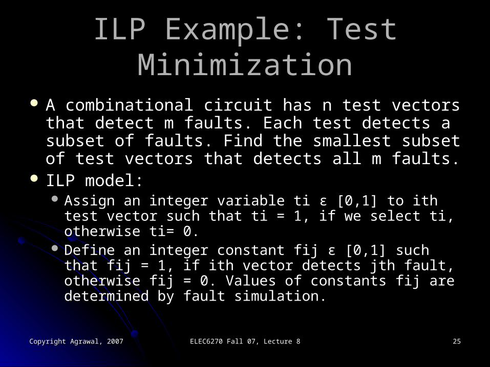
ILP Example: Test MinimizationILP Example: Test Minimization

A combinational circuit has n test vectors that A combinational circuit has n test vectors that detect m faults. Each test detects a subset of detect m faults. Each test detects a subset of faults. Find the smallest subset of test vectors faults. Find the smallest subset of test vectors that detects all m faults.that detects all m faults.

ILP model:ILP model: Assign an integer variable ti Assign an integer variable ti εε [0,1] to ith test vector [0,1] to ith test vector

such that ti = 1, if we select ti, otherwise ti= 0.such that ti = 1, if we select ti, otherwise ti= 0. Define an integer constant fij Define an integer constant fij εε [0,1] such that fij = 1, if [0,1] such that fij = 1, if

ith vector detects jth fault, otherwise fij = 0. Values of ith vector detects jth fault, otherwise fij = 0. Values of constants fij are determined by fault simulation. constants fij are determined by fault simulation.


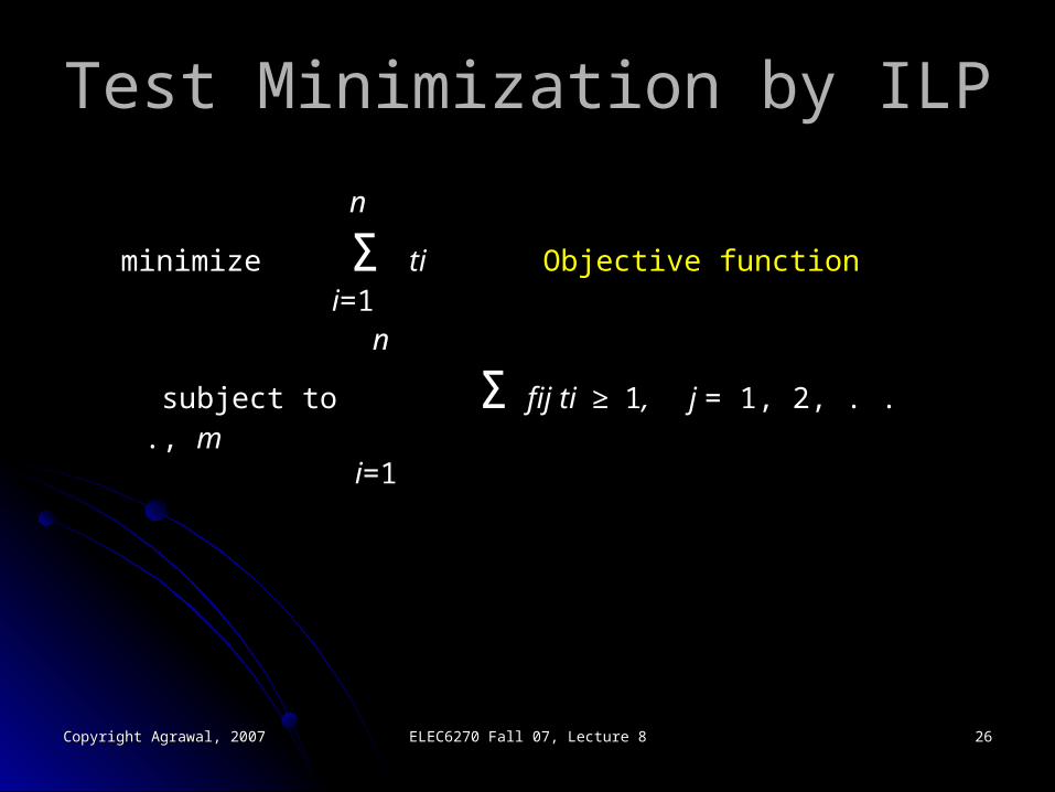
Test Minimization by ILPTest Minimization by ILP

n

minimize Σ ti Objective function i=1 n

subject to Σ fij ti ≥ 1, j = 1, 2, . . ., mi=1


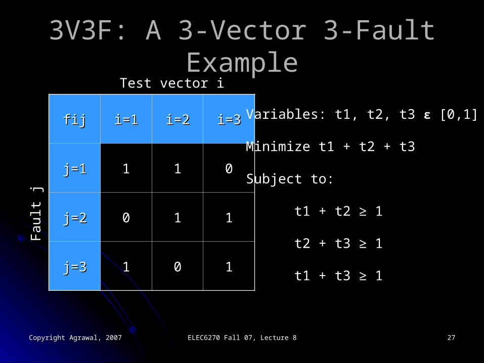
3V3F: A 3-Vector 3-Fault Example3V3F: A 3-Vector 3-Fault Example

fijfij i=1i=1 i=2i=2 i=3i=3

j=1j=1 11 11 00

j=2j=2 00 11 11

j=3j=3 11 00 11

Test vector i

Fau

lt j

Variables: t1, t2, t3 εε [0,1]

Minimize t1 + t2 + t3

Subject to:

t1 + t2 ≥ 1

t2 + t3 ≥ 1

t1 + t3 ≥ 1


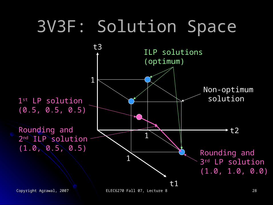
3V3F: Solution Space3V3F: Solution Space

Non-optimum solution

t1

t2

t3

1

1

1

1st LP solution(0.5, 0.5, 0.5)

ILP solutions(optimum)

Rounding and2nd ILP solution(1.0, 0.5, 0.5)

Rounding and3rd LP solution(1.0, 1.0, 0.0)


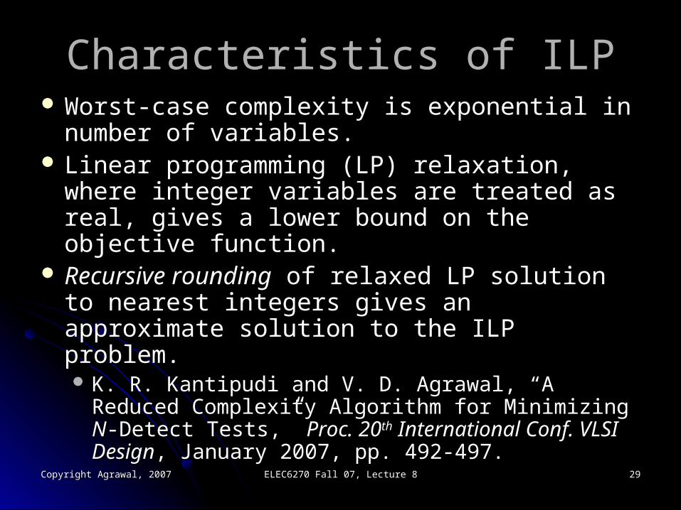
Characteristics of ILPCharacteristics of ILP Worst-case complexity is exponential in number Worst-case complexity is exponential in number

of variables.of variables. Linear programming (LP) relaxation, where Linear programming (LP) relaxation, where

integer variables are treated as real, gives a integer variables are treated as real, gives a lower bound on the objective function.lower bound on the objective function.

Recursive roundingRecursive rounding of relaxed LP solution to of relaxed LP solution to nearest integers gives an approximate solution nearest integers gives an approximate solution to the ILP problem.to the ILP problem. K. R. Kantipudi and V. D. Agrawal, “A Reduced K. R. Kantipudi and V. D. Agrawal, “A Reduced

Complexity Algorithm for Minimizing Complexity Algorithm for Minimizing NN-Detect Tests,” -Detect Tests,” Proc. 20Proc. 20thth International Conf. VLSI Design International Conf. VLSI Design, January , January 2007, pp. 492-497.2007, pp. 492-497.


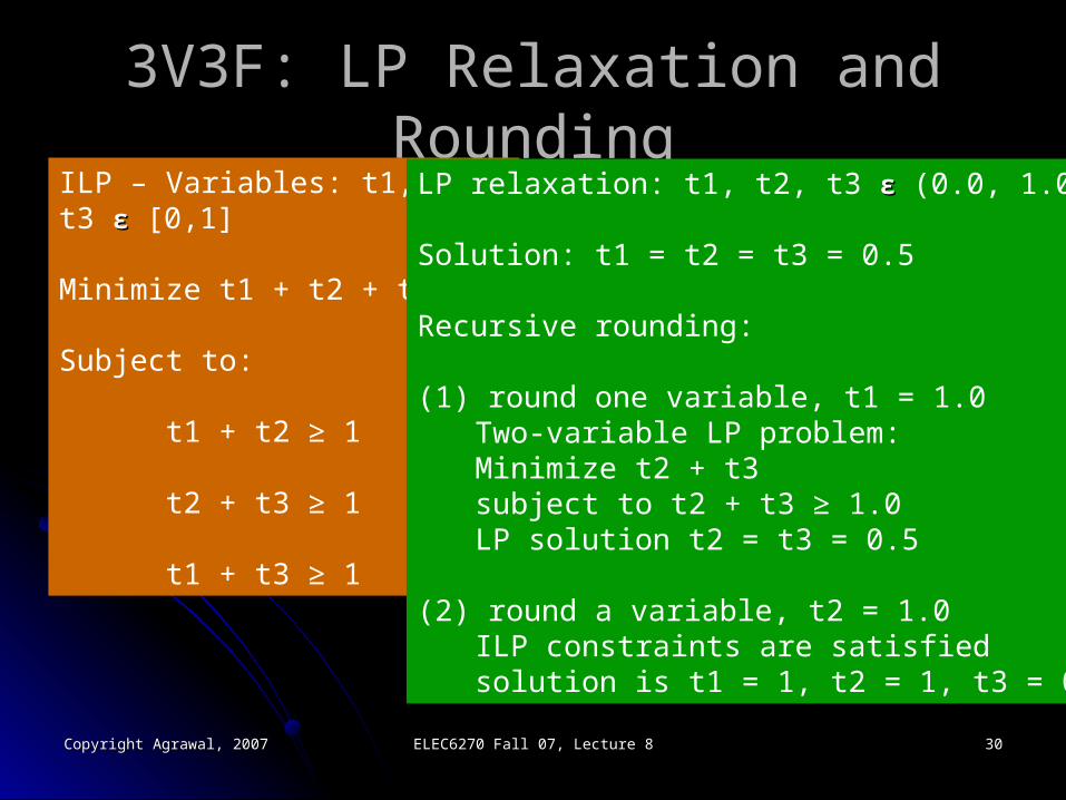
3V3F: LP Relaxation and Rounding3V3F: LP Relaxation and RoundingILP – Variables: t1, t2, t3 εε [0,1]

Minimize t1 + t2 + t3

Subject to:

t1 + t2 ≥ 1

t2 + t3 ≥ 1

t1 + t3 ≥ 1

LP relaxation: t1, t2, t3 εε (0.0, 1.0)

Solution: t1 = t2 = t3 = 0.5

Recursive rounding:

(1) round one variable, t1 = 1.0 Two-variable LP problem: Minimize t2 + t3 subject to t2 + t3 ≥ 1.0 LP solution t2 = t3 = 0.5

(2) round a variable, t2 = 1.0 ILP constraints are satisfied solution is t1 = 1, t2 = 1, t3 = 0


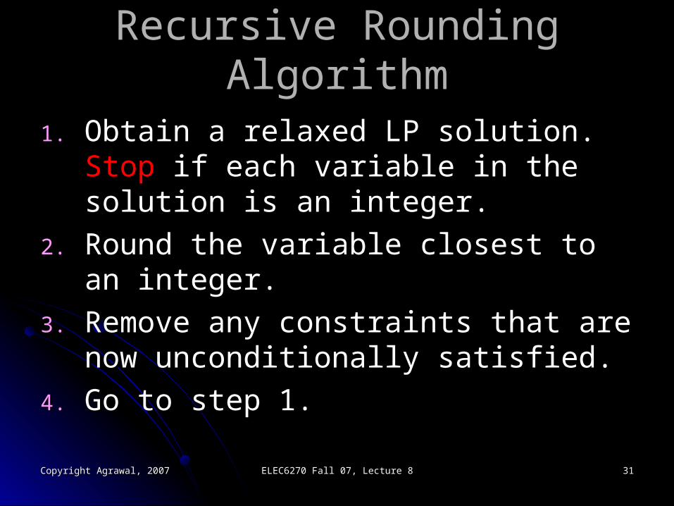
Recursive Rounding AlgorithmRecursive Rounding Algorithm

1.1. Obtain a relaxed LP solution. Obtain a relaxed LP solution. Stop if if each variable in the solution is an each variable in the solution is an integer.integer.

2.2. Round the variable closest to an integer.Round the variable closest to an integer.

3.3. Remove any constraints that are now Remove any constraints that are now unconditionally satisfied.unconditionally satisfied.

4.4. Go to step 1.Go to step 1.


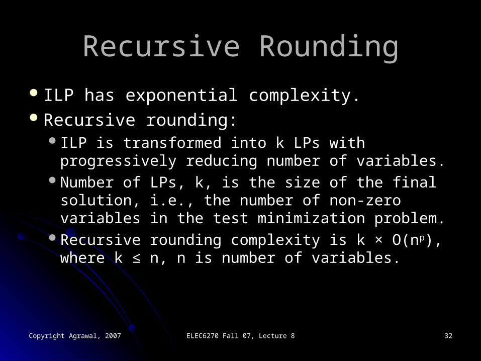
Recursive RoundingRecursive Rounding

ILP has exponential complexity.ILP has exponential complexity.Recursive rounding:Recursive rounding:

ILP is transformed into k LPs with ILP is transformed into k LPs with progressively reducing number of variables.progressively reducing number of variables.

Number of LPs, k, is the size of the final Number of LPs, k, is the size of the final solution, i.e., the number of non-zero solution, i.e., the number of non-zero variables in the test minimization problem.variables in the test minimization problem.

Recursive rounding complexity is k × O(nRecursive rounding complexity is k × O(npp), ), where k ≤ n, n is number of variables.where k ≤ n, n is number of variables.


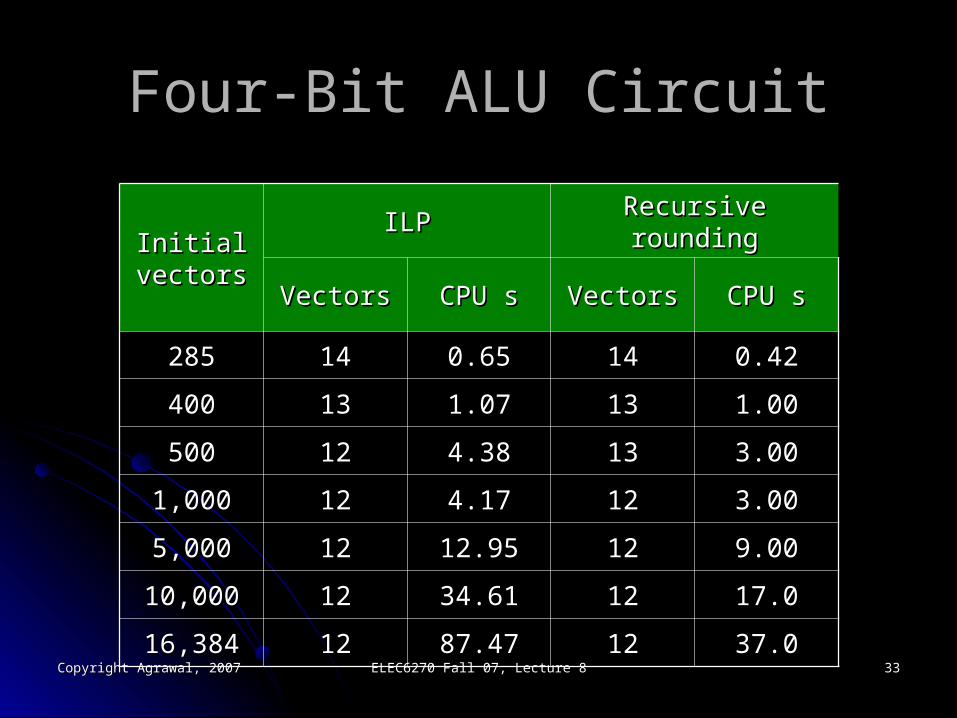
Four-Bit ALU CircuitFour-Bit ALU Circuit

Initial Initial vectorsvectors

ILPILP Recursive roundingRecursive rounding

VectorsVectors CPU sCPU s VectorsVectors CPU sCPU s

285285 1414 0.650.65 1414 0.420.42

400400 1313 1.071.07 1313 1.001.00

500500 1212 4.384.38 1313 3.003.00

1,0001,000 1212 4.174.17 1212 3.003.00

5,0005,000 1212 12.9512.95 1212 9.009.00

10,00010,000 1212 34.6134.61 1212 17.017.0

16,38416,384 1212 87.4787.47 1212 37.037.0


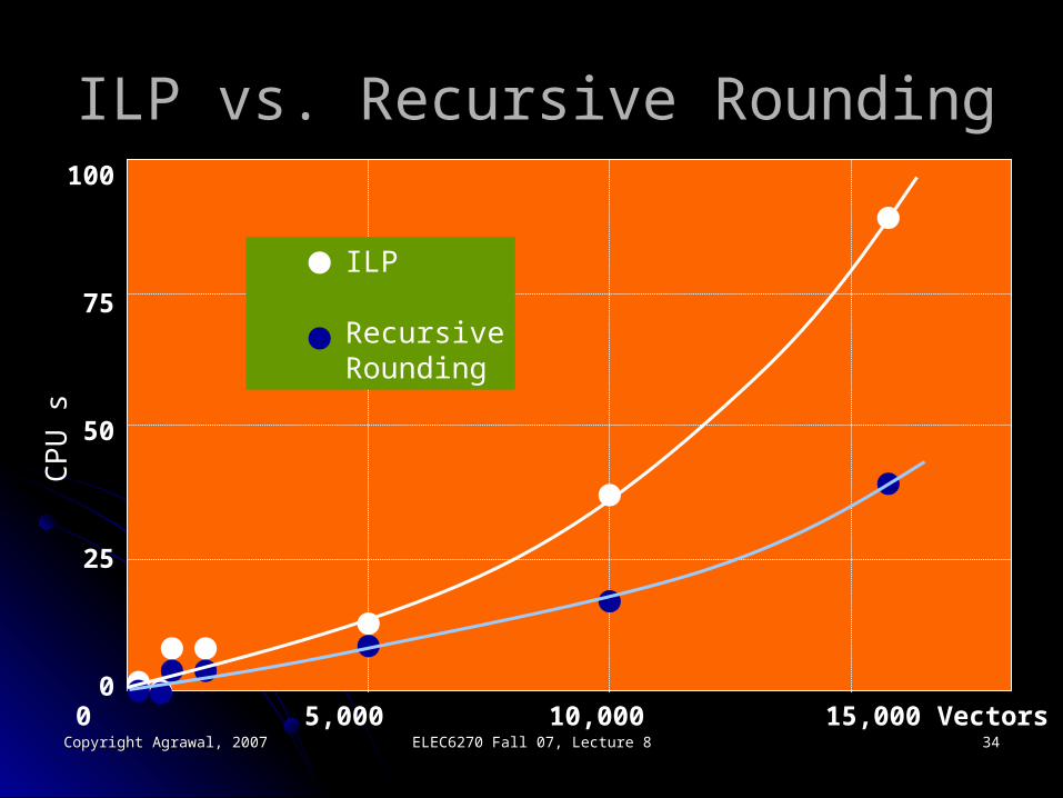
ILP vs. Recursive RoundingILP vs. Recursive Rounding

0 5,000 10,000 15,000 Vectors

100

75

50

25

0

ILP

Recursive Rounding

CPU

s


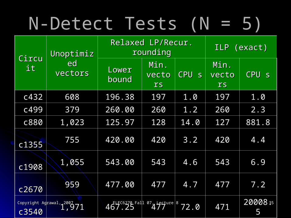
N-Detect Tests (N = 5)N-Detect Tests (N = 5)

CircuitCircuit Unoptimized Unoptimized vectorsvectors

Relaxed LP/Recur. Relaxed LP/Recur. roundingrounding ILP (exact)ILP (exact)

Lower Lower boundbound

Min. Min. vectorsvectors CPU sCPU s Min. Min.

vectorsvectors CPU sCPU s

c432c432 608608 196.38196.38 197197 1.01.0 197197 1.01.0

c499c499 379379 260.00260.00 260260 1.21.2 260260 2.32.3

c880c880 1,0231,023 125.97125.97 128128 14.014.0 127127 881.8881.8

c1355c1355 755755 420.00420.00 420420 3.23.2 420420 4.44.4

c1908c1908 1,0551,055 543.00543.00 543543 4.64.6 543543 6.96.9

c2670c2670 959959 477.00477.00 477477 4.74.7 477477 7.27.2

c3540c3540 1,9711,971 467.25467.25 477477 72.072.0 471471 20008.520008.5

c5315c5315 1,0791,079 374.33374.33 377377 18.018.0 376376 40.740.7

c6288c6288 243243 52.5252.52 5757 39.039.0 5757 34740.034740.0

c7552c7552 2,1652,165 841.00841.00 841841 52.052.0 841841 114.3114.3


Finding LP/ILP SolversFinding LP/ILP Solvers

R. Fourer, D. M. Gay and B. W. Kernighan, R. Fourer, D. M. Gay and B. W. Kernighan, AMPL: A AMPL: A Modeling Language for Mathematical ProgrammingModeling Language for Mathematical Programming, , South San Francisco, California: Scientific Press, 1993. South San Francisco, California: Scientific Press, 1993. Several of programs described in this book are available Several of programs described in this book are available to Auburn users.to Auburn users.

B. R. Hunt, R. L. Lipsman, J. M. Rosenberg, K. R. B. R. Hunt, R. L. Lipsman, J. M. Rosenberg, K. R. Coombes, J. E. Osborn and G. J. Stuck, Coombes, J. E. Osborn and G. J. Stuck, A Guide to A Guide to MATLAB for Beginners and Experienced UsersMATLAB for Beginners and Experienced Users, , Cambridge University Press, 2006.Cambridge University Press, 2006.

Search the web. Many programs with small number of Search the web. Many programs with small number of variables can be downloaded free.variables can be downloaded free.

Copyright Agrawal, 2007 ELEC6270 Fall 07, Lecture 8 1 ELEC 5270/6270 Fall 2007 Low-Power Design of...

Documents

Transcript of Copyright Agrawal, 2007 ELEC6270 Fall 07, Lecture 8 1 ELEC 5270/6270 Fall 2007 Low-Power Design of...