©Copyright 2012 Steven Leo Zafonte
155
©Copyright 2012 Steven Leo Zafonte
Transcript of ©Copyright 2012 Steven Leo Zafonte

©Copyright 2012
Steven Leo Zafonte
A Determination of the Mass of the Deuteron
Steven Leo Zafonte
A dissertation
submitted in partial fulfillment of the
requirements for the degree of
Doctor of Philosophy
University of Washington
2012
Robert S. Van Dyck, Jr., Chair
Gerald Miller
Paul Boynton
Program Authorized to Offer Degree:
Physics

University of Washington
Abstract
A Determination of the Mass of the Deuteron
Steven Leo Zafonte
Chair of the Supervisory Committee:
Prof. Robert S. Van Dyck, Jr.
Physics
We have measured the atomic mass of the deuteron relative to the calibration 6
12C and
4
12C ions and arrived at a value of 2 014 101 778 052 (40) pu for the mass of deuterium and
2 013 553 212 744 (40) pu for the mass of the deuteron. The spectroscopy was performed in
the new University of Washington Penning Trap Mass Spectrometer (UW-PTMS). The
measurement was made by using the experiment to make a very accurate determination of
the cyclotron frequency of a deuteron isolated in a Penning trap, followed by the cyclotron
frequency of a carbon calibration ion, isolated at the same place in that same trap. The ratio
of the cyclotron frequencies is inversely proportional to the ratio of the two ion’s mass-to-
charge ratio after systematic corrections are made. The deuteron mass along with the proton
mass, which also has its best measurement at the UW-PTMS, can be used with the deuteron
binding energy[20] to refine the neutron mass to 1 008 664 916 018 (435) pu.nm
In addition to discussing the physics of our penning trap spectrometer and the
systematic corrections necessary to obtain a mass ratio, improvements to the spectrometer
will be described that were used in the deuteron measurement as well as improvements that
were made later for future measurements.

i
TABLE OF CONTENTS
Page
List of Figures………………………………………………………………………….. iii
List of Tables…………………………………………………………………………… v
Chapter I: Introduction..................................................................................................... 1
History……………………………………………………………………. 1
The Instrumentation………...……………………………………………. 3
What the Data and Analysis Look Like………………………………….. 4
Chapter II: First Order Physics…………………………………………………………. 8
The Normal Modes of a Particle in a Penning Trap…………………........ 8
Magnetic Field Stability: Magnet Cryostat Design…………………….… 13
Other Passive and Active Magnetic Field Stabilization Systems…..…..... 17
Chapter III: Derivatives of First Order Physics………………………………………… 24
Particle Damping and Driving…………………………………………… 24
Detection System, Lock Loop, Signal Chain Electronics…………..……. 30
Front End Noise…………………………………………………..………. 37
Note on Amplifier and Particle Noise………………………….………… 43
Front End Electronics, Old and New…………………………..…………. 46
Chapter IV: Higher Order Physics and Implications…………………………………… 51
Coupling to the Cyclotron Mode…………………………………..……... 51
Relativistic Pulling, the Cyclotron Resonance, and the Range Effect…..... 56
Ion Centering and Magnetron Frequency Measurement………………..... 59
Perturbations from Residual Mode Energy and Axial Systematic…….… 65
Image Charge Effect………………………………………………….…... 66
Ion-Ion Interactions, Ion Loading, and Ion Cleaning……………….……. 68
Chapter V: Data, Analysis, and Results…………………………………………….….. 83
Data Analysis and How the Systematics Were Applied…………….…… 83
Run Analysis……………………………………………………….…….. 88
Analysis Summary and Conclusions…………………………….……….. 100
Chapter VI: Experimental Improvements and Assorted Subsystems……………..……. 102
Full Experiment Topology and Frequency Synthesis…………….……… 102
Standard Cell Ring Voltage Source and RC Stabilization System.……… 105
Helium Pressure and Level system…………………………….………… 113
New Field Trim Coil………………………………………….………….. 119
Helical Resonator Coil Trimming Circuit………………….…………….. 120
High Voltage Current Limiter……………………………………………. 122
100 kHz Multiband Amplifier……………………………………………. 123

ii
TABLE OF CONTENTS
Page
Bibliography……………….…………………………………………………………... 126
Appendix A: Experimental Parameters…………………………………..……………. 127
Appendix B: Computer Code………………………………………………………….. 130

iii
LIST OF FIGURES
Figure Number Page
1.1 Penning Trap………………………………………………………………. 2
1.2 Experiment Layout………………………………………………………… 4
1.3 Cyclotron Sweeps…………………………………………………………. 5
1.4 Representative Cyclotron Data Residuals…………………………………. 6
2.1 Normal Modes in a Penning Trap………………………………………… 9
2.2 Cryostat……………………………………………………………………. 15
2.3 Trolley Magnetic Field……………………………………………………. 18
2.4 Flux Gate Magnetometer Probe…………………………………………… 20
3.1 Axial Resonance…………………………………………………………… 28
3.1 Simplified Lock Loop Topology………………………………………….. 31
3.2 Base Band Loop Dynamics……………………………………………….. 34
3.3 Loop Transfer Function…………………………………………………… 35
3.4 Helical Resonator…………………………………………………………. 38
3.5 Simplified Front End……………………………………………………… 39
3.6 Feedback Noise……………………………………………………………. 41
3.7 FET Modules……………………………………………………………… 47
4.1 Field Trim Coils…………………………………………………………... 54
4.2 Current Source……………………………………………………………. 55
4.3 Downsweep Resonance…………………………………………………… 57
4.4 Upsweep Resonance………………………………………………………. 57
4.5 Range Effect………………………………………………………………. 58
4.6 Magnetron Cooling Resonance……………………………………………. 61
4.7 Cyclotron Coupling Resonance……………………………………………. 63
4.8 Image Charge Effect……………………………………………………… 67
4.9 Ion Loading……………………………………………………………….. 74
4.10 Slow Drop Circuit………………………………………………………… 78
4.11 Fast Drop Circuit………………………………………………………….. 79
5.1 Axial Systematic………………………………………………………….. 84
5.2 Histogram of Sweep Supervisor Error Bars………………………………. 87
5.3 Summary of Runs…………………………………………………………. 89
5.4 Run #1 Residuals………………………………………………………….. 90
5.5 Run #2 Residuals………………………………………………………….. 91
5.6 Run #6 Residuals………………………………………………………….. 92
5.7 Run #8 Residuals………………………………………………………….. 93

iv
LIST OF FIGURES
Figure Number Page
5.8 Run #9 Residuals………………………………………………………….. 94
5.9 Run #10 Residuals………………………………………………………… 95
5.10 Run #11 Residuals…………………………………………………………. 96
5.11 Run #12 Residuals…………………………………………………………. 97
5.12 Run #13 Residuals………………………………………………………… 98
5.13 Run #14 Residuals………………………………………………………… 99
6.1 Full Experiment Topology………………………………………………… 103
6.2 Improved Experiment Topology………………………………………….. 104
6.3 Battery Distribution System………………………………………………. 107
6.4 RC System Noise Transfer Function……………………………………… 111
6.5 RC Ring Stabilization System…………………………………………….. 112
6.6 Cyclotron Frequency vs. Barometric Pressure……………………………. 114
6.7 Helium Level Control System…………………………………………….. 115
6.8 Helium Level Sensor Oscillator Driver…………………………………… 117
6.9 Helium Boil-Off Gas Handling System…………………………………… 118
6.10 Improved Magnetic Field Shimming Coils……………………………….. 119
6.11 Helical Resonator Trimming Circuit…..…………………………………. 121
6.12 High Voltage Current Limiter……………………………………………. 122
6.13 100 kHz Dual Band Amplifier……………………………………………. 124

v
LIST OF TABLES
Table Number Page
5.1 Run Results with Systematic Shifts……………………………………….. 88
A.1 Experimental Parameters…………………………………………………. 129

vi
ACKNOWLEDGEMENTS
It has been a privilege to work with Prof. R. S. Van Dyck and Prof. P. B. Schwinberg. They
lured me away from my planned career in solid state physics with a lab that had a habit of
turning difficult ideas into elegant experimental realities. I do not have higher praise and their
tutelage has contributed greatly to the versatility of my problem solving ability.
I would also like to acknowledge the help and patience of my family under what were very
unusual circumstances. Without them, I would not be here.

1
Chapter I: Introduction
Section I.1: History
A Penning trap makes a combination of magnetic and electric fields which is capable
of “trapping” a charged particle in a region of space for an extended period of time. In their
original form, they were used as a way of enhancing a gas discharge by F.M. Penning in
1936 [1]. They have progressed in crude forms to make gages and pumps important to
current vacuum technology. More carefully constructed penning trap experiments are used in
the fields of Chemistry, Physics, and Biology to do both metrological and analytical mass
spectroscopy on trapped charged particles. Highly refined versions of the Penning traps have
been used to measure the magnetic moment of the electron and the positron [2] [3]. This was
central in the work that led to the Physics Nobel Prize in 1989 by Hans Dehmelt at
University of Washington.
Penning trap experiments owe their genesis to the work of Prof. Dehmelt in the
1950’s when crude traps made of metal screen were used to capture clouds of electrons.
These were used to make electron g-2 measurements at the 1% level [4]. By making a trap
with solid electrodes and adding guards to shim out electrical anharmonicity, single particles
were resolved for the first time in 1976 with new, more harmonic traps [5].
The first penning trap ion mass spectroscopy, though not technically an ion mass
comparison, was done with the original quad-ring UW Penning Trap Mass Spectrometer to
find the proton/electron mass ratio in the 1986 [6]. This was a 20 ppb measurement. The first
true ion mass with carbon as a reference, without the complications of dealing with an
electron, was done in 1988, on the proton with an accuracy of 3 ppb [7]. This measurement
was refined in 1993 to the 1 ppb accuracy level [8]. Next, the Penning trap mass
spectrometry technique was leveled at calculating the 3 3H He mass difference. This can
be used to calculate the mass of the electron neutrino if done with sufficient accuracy and
combined with the 3H beta-decay endpoint energy [9] [10]. In 1995, with a new Penning
trap technique based on electric anharmonicity instead of a magnetic bottle, the
proton/electron mass ratio was measured again, this time with an accuracy of 2.2 ppb [11].
Several ions have had precision mass spectroscopy performed on them in the past years
2
leading up to our measurements on deuterium and 3He . Currently, the best metrological
spectroscopy experiments are the UW-PTMS experiment, now moved to Mainz, Germany
[12] [13] [14], and the MIT machine [15] [16], now at Florida State University [17] [18]
[19]. These newest machines turn out numbers 3 orders of magnitude better than the first
measurements.
In this monograph we present the measurement of the atomic mass of the deuteron.
This is listed among the fundamental constants by NIST and it can be used to determine the
neutron mass, another fundamental constant. The deuteron mass is also used as a yardstick by
other groups to make other measurements [20]. In this example the group of interest is using
our preliminary number from the current measurement.
3
Section I.2 The Instrumentation
In the following two sections I will give a quick overview of the experiment. A
hyperbolic Penning trap is a device which confines a charged particle in a combination of a
strong axial magnetic field and an electric field whose potential approximates an electric
quadrupole. In our case, the electric field is created by electrodes shaped as hyperboloids of
revolution, the equipotential surfaces of that electric quadrupole. As long as you occasionally
apply a centering drive called a “cooling” drive (radial confinement is metastable though
long-lived) a charged particle can be stored for as long as the experimenter has patience. The
guard electrodes are split in two half rings to allow this, and all other drives to be applied
across the trap.
The UW-PTMS is a system with a Penning trap at its center and capable of making
comparisons of the free space cyclotron frequencies of light ions to a few parts in 1110 . It
consists of a single compensated hyperbolic Penning trap kept in a vacuum. At the center of
this Penning trap (figure 1.1) is the ion of interest. Image currents of the ion’s motion are
detected at the signal endcap of the Penning trap and its motion is driven from RF (radio
frequency) voltages applied to the opposite endcap, the drive endcap, at a motional sideband
of particle’s natural axial frequency opened up by a ring electrode modulation RF voltage.
The particle is put into the Penning trap during the ion loading process. This consists
of pulling an electron beam from the tungsten field emission point via a voltage difference
relative to the near skimmer. The beam crosses the trap and is folded back by the reflector
electrode. This provides enough high energy electrons to scrub atoms adsorbed on the
skimmers off into the trap and sequentially ionize them to make the charge state desired.
The trap is encased in a beryllium copper vacuum envelope. It, along with the
preamplifier, and associated electronics are submerged in liquid helium in the center of a
custom designed ultra-stable superconducting solenoid and cryostat system [21] generating a
nearly uniform 5.9T field and supplying a passive magnetic noise shielding system giving
about a factor of 200 isolation from external magnetic field disturbances. The cryostat is
placed within an active magnetic field stabilization system which reduces external magnetic
noise by another factor of about 50. This in turn is placed in an aluminum shield room to give
high frequency RF electromagnetic shielding. This shield room is placed in a pit which

4
thermally and vibrationally isolates it as much as is practical from the building environment.
The control electronics that do not need temperature stabilization reside in racks outside the
shield room and roughly 2 m over and 2 m up from the magnet center. From here, the
experimenter operates the apparatus (figure 1.2).
Section I.3 What the Data and Analysis Look Like
The free space cyclotron frequency of a charged particle in a magnetic field is given
by the following equation:
.c
qB
m (1.1)
5
This is a rough approximation of the real trapped case where the magnetic field is
modified by the trapping electric field giving a modified cyclotron frequency from which the
free space number can be derived if the two other normal mode frequencies (see section II.1)
are known. By comparing the free space cyclotron frequency of two species of ion, in this
case, the deuteron with 6
12C or 4
12C , one can find their mass ratio from the CFR (Cyclotron
Frequency Ratio) as follows:
,
,
.c D D C
c C C D
q mCFR
q m
(1.2)
Most of the time, the experiment is taking successive cyclotron excitation RF drive
sweeps up then down in frequency looking for the cyclotron resonance. By these sweeps the
position of cyclotron resonance is bracketed. The measurement of the trap cyclotron
frequency is taken to be half way between the start corner of the respective up and down
excitations. An example of a pair of sweeps is shown in Fig. 1.3. A run usually consists of a
few hundred pairs of sweeps of2D , followed by a few hundred pairs, taken at almost exactly
the same

6
field, for the calibration ion, either a 6
12C or a 4
12C . An example of the residuals for one of our
runs is shown in figure 1.4. Note that the scatter for carbon is much smaller than that of
deuterium. This is because the carbon has a higher charge state and is easier to detect.
Note: 12C is used because the atomic mass unit (amu) is defined such that it has a mass of
exactly 12 amu. The experiment’s magnetic field is not truly constant, but because we have
taken great pains to stabilize it, it executes a near linear drift with a slight quadratic at a few
tenths of a ppt/h which can be fitted out. After each cyclotron sweep, centering drives are
applied to prepare an unexcited initial state of the ion at the center of the trap with cyclotron
energy below 30 meV. This residual energy contributes only +/- 5ppt to the uncertainty of the
measurement from the extra relativistic mass it contributes to the deuterium or carbon ion.
From the measured CFR (cyclotron frequency ratio) and by adding the mass of the electrons
necessary to bring the ion back to neutral, along with the total relativistic mass of the binding
energy, the mass of deuterium can be arrived at by the following equations:
6
2
2
4
2
2
12 6
6
12 4
,4
C
bindDC ebind
D e
C
bindDC ebind
D e
Em m
Ecm mCFR c
Em m
Ecm mCFR c
(1.3)

7
where the first equation is for a comparison between the deuteron and 6
12C and the second is
for a comparison between the deuteron and 4
12C .
In addition to the deuteron mass, which is listed among the NIST fundamental
constants, the results presented here can be used to determine the neutron mass. If one
examines the following reaction:
2 1D E H n
(1.4)
which represents the gamma ray dissociation of the deuterium nucleus, it is easy to see that
you can arrive at a neutron mass:
2
.n D H
Em m m
c
(1.5)
We have now measured both the deuteron and the proton [11] mass. The gamma ray binding
energy of the deuteron has been measured by Kessler [22], thus completing the equation.
The measurement of the deuteron mass presented in this work improves upon the next
best measurement in the past by a factor of 15 [23].
8
Chapter II: First Order Physics
Section II.1: The Normal Modes of a Particle in a Penning Trap
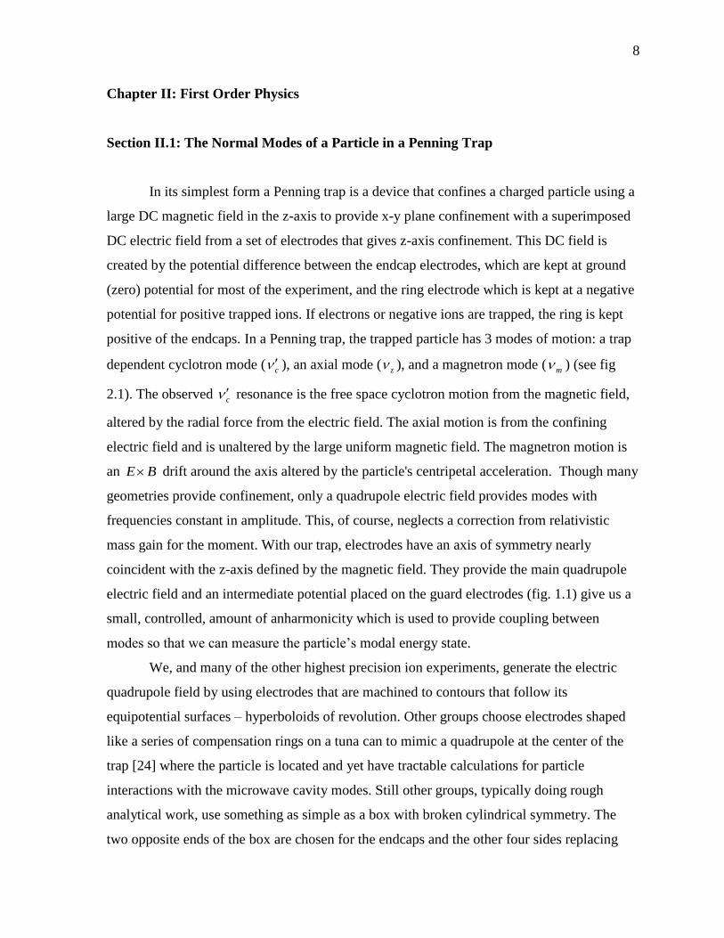
In its simplest form a Penning trap is a device that confines a charged particle using a
large DC magnetic field in the z-axis to provide x-y plane confinement with a superimposed
DC electric field from a set of electrodes that gives z-axis confinement. This DC field is
created by the potential difference between the endcap electrodes, which are kept at ground
(zero) potential for most of the experiment, and the ring electrode which is kept at a negative
potential for positive trapped ions. If electrons or negative ions are trapped, the ring is kept
positive of the endcaps. In a Penning trap, the trapped particle has 3 modes of motion: a trap
dependent cyclotron mode ( c ), an axial mode ( z ), and a magnetron mode ( m ) (see fig
2.1). The observed c resonance is the free space cyclotron motion from the magnetic field,
altered by the radial force from the electric field. The axial motion is from the confining
electric field and is unaltered by the large uniform magnetic field. The magnetron motion is
an E B drift around the axis altered by the particle's centripetal acceleration. Though many
geometries provide confinement, only a quadrupole electric field provides modes with
frequencies constant in amplitude. This, of course, neglects a correction from relativistic
mass gain for the moment. With our trap, electrodes have an axis of symmetry nearly
coincident with the z-axis defined by the magnetic field. They provide the main quadrupole
electric field and an intermediate potential placed on the guard electrodes (fig. 1.1) give us a
small, controlled, amount of anharmonicity which is used to provide coupling between
modes so that we can measure the particle’s modal energy state.
We, and many of the other highest precision ion experiments, generate the electric
quadrupole field by using electrodes that are machined to contours that follow its
equipotential surfaces – hyperboloids of revolution. Other groups choose electrodes shaped
like a series of compensation rings on a tuna can to mimic a quadrupole at the center of the
trap [24] where the particle is located and yet have tractable calculations for particle
interactions with the microwave cavity modes. Still other groups, typically doing rough
analytical work, use something as simple as a box with broken cylindrical symmetry. The
two opposite ends of the box are chosen for the endcaps and the other four sides replacing

9

10
our ring electrode. Frequently in these traps the excitation and detection of the cyclotron
motion are done on alternate faces of the cube where our ring electrode would be.
For the general trap with cylindrical symmetry and a zero potential at the center of the
trap, the electric potential can be expressed:
0
0
cos .2
l
l l
l
V rV C P
d
(2.1)
If the trap is properly engineered, it is symmetric about the z=0 plane and all lC where l are
odd disappear. The most important terms at the center of the trap are lC where 2,4l . For
the case of a perfect quadrupole trap, only 2C is non-zero. I will deal with small,
intentionally introduced 4C terms later as they are critical for the operation of the
experiment.
Let me examine the non-relativistic dynamics of this case more carefully. First, the
potential is:
2 2
202 22 2
cos 3cos 1 .2
Vr rC P
d d (2.2)
In cylindrical coordinates it becomes:
2 2
0
2
2
2 2
V z
d
(2.3)
where
2
2 00
12.11
22d z mm
(2.4)
for our trap. 0z equals half the distance between the endcaps and is 2.28 mm. 0 equals the
inner radius of the ring electrode and is 2.74 mm.
The axial magnetic field is 0ˆ5.9B zT . Clearly the motion in the z direction
decouples from the magnetic field and we get the familiar harmonic potential:
2
0
22
V zV z
d
(2.5)
and sinusoidal motion with a frequency:

11
2 0
2z
V q
md (2.6)
where q/m is the charge-to-mass ratio for the ion.
Next I will solve for the motion in the x-y (or , ) plane in a cylindrical coordinate
system rotating at frequency . [Please forgive the non-standard approach; however it will
be useful later. ( qB m is the free space cyclotron frequency c )]
Ignoring the ̂ motion, the force and composite motion on and of the particle are:
2
00 02
ˆ ˆˆ2 2
zc
VF q E v B z q B m m
d
(2.7)
2
2 2 ˆ ˆ2 .2
zcma F
(2.8)
For a single stable mode 0 and set 0 to solve for an where the particle rotates at
the same rate as the coordinate system:
2 222
20 .
2 2
c c zzc
(2.9)
We shall call c , the modified cyclotron frequency, and we shall call m , the
magnetron frequency. First, note that as the square root term becomes imaginary for
2 ,z c (2.10)
there are no longer stable particle orbits (where 0 ) where this inequality holds. This puts
limits on how large a mass of atom can be sequentially ionized at a given ring potential (i.e.
one needs2 2
0
2m B d
q V .) These limits are not very serious for our experiment; in fact they
may even prevent sputtered tungsten from entering our trap during the ion loading process
because the heavy singly ionized species would leave the trap before it could become more
ionized than the ion of interest and displace it. It would be a serious limit for Chemists and
Biologists who load proteins into Penning traps to do analytical spectroscopy on mixtures. In
practice, the hierarchy is maintained
12
with
.079 and .040
c z m
mz
c z
(2.11)
for this experiment.
Two further equations to note are:
c c m (2.12)
and
2 2 2 2 .c c z m (2.13)
The first equation is just approximately true, being exact only when the axis of symmetry of
the electric field is lined up with the z-axis determined by the B-field. Again, we take pains
on alignment, adjusting the two axes to less than one milliradian. The second equation (the
quadrature relation) is true in spite of misalignments [25] and certain electrode imperfections.
It is used for all the highest precision spectroscopy. By taking the differential of the
quadrature equation we get:
c mzc c z m
c c c
d d d d
(2.14)
and
2 2 2
.c c c m mz z
c c c c z c m
(2.15)
These equations are useful when a systematic causes a discrepancy of the true normal mode
frequency from the measured normal mode frequency. For example, though the magnetron
frequency is measured routinely only to a few mHz, its impact on the final measured
cyclotron frequency is negligible due to the scaling of the factor .003m
c
.
Here is a list of the normal mode frequencies in the deuteron experiment:

13
612 2
412
,
452
302
3.552
0.14 .2
C D
C
c
c
z
m
MHz
MHz
MHz
MHz
(2.16)
The magnetron motion is metastable because it is at the top of an electrical potential
hill at the center of the trap and the energy goes down as the magnetron radius increases.
Thankfully, in the normal course of the experiment the magnetron mode is not excited, and
the lifetime is long enough that we do not notice it unless the centering drive is accidentally
left off for a few days.
Section II.2 Magnetic Field Stability: Magnet Cryostat Design
Eq. 1.2, ,
,,D C
C C D
c D
c
q m
q m
presupposes that the magnetic field does not change during
the measurement. At some level this is, of course, untrue. A change in the magnetic field at
trap center that lowers it by one part in 1011
(or 0.59 G out of 59 KG) during the time that
the calibration ion is loaded lowers the measured mass of the ion of interest by one part in
1011
. Thankfully comparisons of one carbon ion to another carbon ion, even with a different
charge state, yield a fitted mass ratio of 1, and are consistent with no systematic shift during
the ion loading process. The magnetic field does change over the run as the cryogen levels in
the outer and inner storage tanks lower. This drift is fit to a linear and quadratic polynomial
with much of the uncertainty coming from our inability to distinguish between the two
models. Both, however, are smooth and analytic, and not really a source of magnetic field
uncertainty. Instability would manifest itself in magnetic field variations that are departures
from smooth curves. In this section I will describe the methods used to control the magnetic
field. The experiment was performed after the magnet has settled for a few years. At that

14
point the overall field drift has been observed on occasion to be less than 0.100 ppt/hr.
First and most important to magnetic field stability, is our custom designed 5.9T
superconducting magnet/cryostat and experiment design, a more thorough treatment can be
found here [21]. The field of any magnet will have inhomogeneities at its field center. This
one has a uniformity of 2 parts in810 over 1 cm as measured by a spherical NMR probe. Any
movement of the experiment relative to the magnet center will show up as a field shift.
Luckily, keeping this constant to the 5 microns necessary to achieve 1 part in 1011
accuracy
seems to be achievable, or at the very least, any variation is smooth with time and can be fit
out. Additionally, since the magnetic susceptibility of the G-10 epoxy/glass composite bore
tube is proportional to 1T , variations become large at low temperatures [26], and it becomes
important to keep all the high field parts of the experiment at a stable temperature.
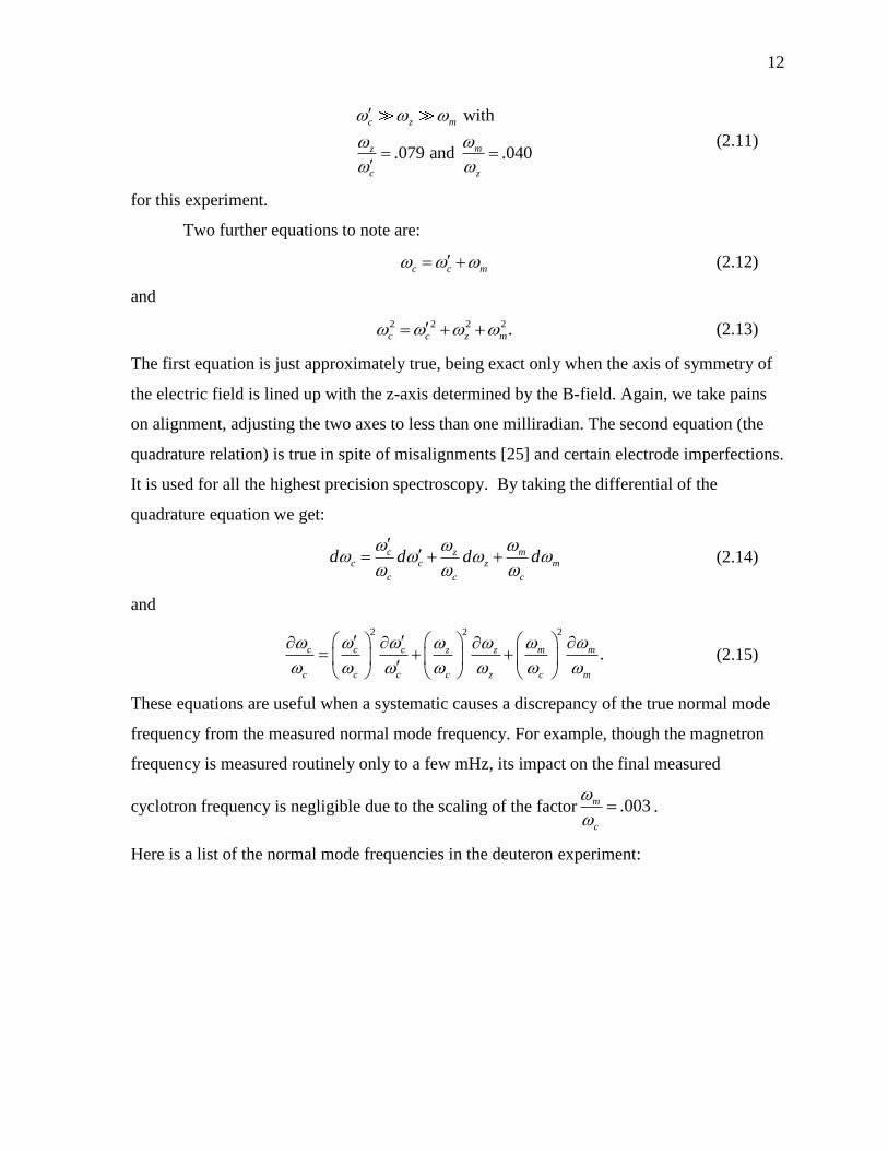
A magnet/experiment diagram is shown here in fig 2.2. The magnet is designed so
that both the magnet solenoid and the experiment are anchored at the same spot, the top of
the dewar's neck. From here, the bore tube of the magnet goes down and directly supports the
solenoid's bobbin. This is unlike standard superconducting magnet designs which have a
vacuum space between the bore tube and the bobbin to allow the bore to be thermally
isolated from the superconducting magnet. This standard design is used for room temperature
bores in magnets designed for nuclear magnetic resonance measurements (of which these
magnets are an offshoot). The lower part of the bore tube is kept at liquid helium
temperatures by the same cryogen that cools the experiment. In a room temperature bore
magnet, both an inner and outer bore tube would not easily get the necessary regulation since
they are not in thermal contact. We had an older magnet made by the same manufacturer
with the room temperature bore design and the new design is considerably (and with further
improvements, increasingly) better (and has become the world’s most stable magnet.)
In the present design, the entire column is temperature stabilized by keeping liquid
helium in it well above the high field region and then temperature controlling the top of the
column. The liquid helium level is measured using one of our own capacitive sensors and
placing it in a feedback loop to control it to better than 40 .m The pressure of the helium gas
column over the liquid is kept constant by locking it to the pressure in a
15

16
temperature controlled absolute pressure reference (APR) filled with a dry gas volume,
temperature controlled to about 1mK. Since the boiling point of helium is temperature
dependent, this stabilizes the temperature at the level of the gas/liquid interface.
All this provided a field that changed very little with environmental effects that
change the external pressure or temperature. However, recently we have further improved the
cryostat (after the Deuterium measurements). We noticed that the sign of the atmospheric
pressure coefficient changes when a 2”x3” aluminum bar is bolted to the experiment header
and the magnet cryostat’s 1.5” thick top plate. We therefore surmised that by connecting the
bar to the experiment with a “spring” of the appropriate stiffness, we would be able to null
out this dependence. In fact, by creating a jig with a very stiff “spring” made from the
appropriate thickness of stainless steel threaded rod of an adjustable length to fine tune the
spring constant, we were able to cancel out the atmospheric pressure effect to such a level
that we can no longer see any dependence in the data. It is entertaining to note that most of
the adjustments needed to be made during the late fall to early winter. This was because that
was the only time when storms would cause large, rapid pressure changes, and leaving the
other seasons for data taking. Roll out those lazy, hazy, crazy days of summer; those days of
soda, and pretzels, and mass comparisons.
Another source of magnetic field variability has shown up recently, well after the
Deuterium measurement. It seems to have started after we got a bad batch of liquid helium in
2004. Before this we would have on the order of three weeks of stable run time, after which
the drift rate of the field would increase by a factor of five. We assume this is when the liquid
helium level boils below the splices in the superconducting wire made when the magnet was
wound. After that, the stable time decreased, eventually to as little as 10 days. After
spending some time trying to find the cause of this, we hypothesized that the extra variability
was being caused by paramagnetic oxygen ice that was getting stirred up in the magnet. On
checking the helium stacks, it was indeed found that one did have a great deal of air ice in it,
and after melting it out with a hot (room temperature) aluminum rod, the magnet stability
greatly improved again. We now clear the stacks every time there is a liquid helium fill. It is
very likely that at the part in 1011
level and below, oxygen ice in the magnet will become an
increasingly important problem.

17
Section II.3 Other Passive and Active Magnetic Field Stabilization Systems
In addition to magnetic field changes from sources internal to the magnet, there are
also magnetic field changes that come from the surrounding environment. Local field
changes from sources such as the movement of steel furniture can be mitigated. During a run,
every metal chair has is place, lab cranes are parked, and my desk chair (which was close to
the magnet) was always made of wood. The effect of metal objects in the immediate vicinity
of the magnet falls off as “induced dipoles”. To first order, the magnet itself is a dipole
whose field falls off as 31 r , which induces a dipole in the ferromagnetic object that is
proportional to the original field and roughly proportional to the square of the characteristic
length of metal in the direction of the field lines. Note this only applies to rather soft steels.
Harder steel, for example, racing bicycle frame tubes, have much smaller characteristic
lengths since the lower permeability of their metal is unable to pull in enough field to deform
it out to a distance of the characteristic length. The dipole moment of the offending object
falls off again as 2 3l r leading to the overall 2 6l r magnetic disturbance back at the field
center. In the next zone, where the earth's magnetic field becomes larger than the field from
the magnet (greater than about 4 meters) the offending disturbance falls off as 2 3l r . Before
the magnet was installed, some time was spent measuring the effects of objects moving in
this far field with a sensitive magnetometer where the magnet center was soon to be placed.
They were found to be negligible for most common objects that would have been of concern.
A notable exception was when the neighboring lab decided to move the steel shelves they
had put against the wall about 4 meters from the magnet. Luckily the effects were very
evident in the flux gate magnetometer’s monitor signal and the event was not frequently
repeated.
In addition to disturbances in the physics building where the experiment is located,
there are much more important sources of magnetic noise - those generated by the world
external to the lab. In 1994 the UW-PTMS was moved from a building in the center of the
UW campus to the new Physics building near the edge of campus. There had been occasional
changes in the earth's magnetic field that impacted the old experiment. That field can vary by
several mG in the case of extremes of solar weather. But these storms are rare and one could
avoid taking data during them if one needed to. What was more important was that the
18
experiment had moved much closer to 15th
Ave./Pacific St. and the unbalanced currents from
the electric trolleys that ran on the street. At first the magnetic noise was in the 7 mG peak-
to-peak region which was over 20 times worse than at the old physics building in the center
of campus.
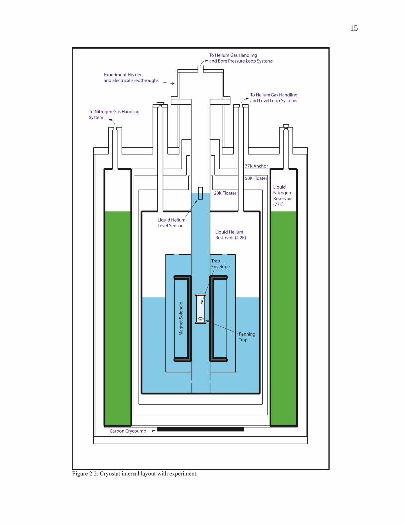
This was addressed in several ways. The first of which was to reduce the problem at
its source. When the outbound and return currents are on opposite sides of a field point, the
magnetic fields from the two currents add to make a larger magnetic field as shown on the
left in figure 3.2. In this case the field falls off as 1/r or worse because the return current is
actually flowing around (and through) the building. Instead when the outbound and return
currents are close together, as in a linear dipole, the fields cancel and the fall off as 1/r2. The
ground return currents had been shunted back haphazardly through the earth (and through our
building) at various points along the trolley line. This problem was solved with the
cooperation of the City of Seattle by making a simple modification to the lines so that the
current returns in the ground line only a meter from the outgoing line. This reduced the
magnetic noise at the physics building down to 1 mG peak-to-peak. Subsequently we have
had continued discussions with the city to keep the magnetic fields from a much larger transit
system which is now under construction to about the same levels so that precision

19
experiments all over campus can still be performed.
1 mG peak-to-peak is still about 15 ppb of noise, much larger than the 55 ppt scatter
that has been seen in the recent data, so much more is necessary to reduce the magnetic
noise. The next step is to create an active field compensation system. This work was started
in collaboration with Prof. Steven Lamreaux, though branched off when the probes became
good enough for our purposes.
The overall system is shown in figure 1.2. It consists of an octagonal Helmholtz coil
surrounding the magnet whose axis parallels the axis of the superconducting solenoid, a flux
gate magnetometer probe placed about 2.5 meters away in a field of 3 mG, and a controller
box which runs the system. Prof. Paul B. Schwinberg designed the system with its
electronics, and I designed the probe. The purpose of the coil is not to null out the earth's
field, since this requires much more power and would be prone to errors in angle between the
probe and the Helmholtz coil. We are only using the system to smooth out the variations in
the experiment's magnetic field from distant sources. By experimenting with the system
before the magnet was in place, we were able to get field variation cancellations better than
75-80. The probe placement 2.5 meters from field center gave a cancellation of better than
50, and was eventually chosen because its lower ambient field.
Since our home made fluxgate magnetometer compensation system decreased
magnetic noise by about a factor of 50, I will explain a little bit about how they work and the
design necessities for our application. A flux gate consists of a closed loop of ferromagnetic
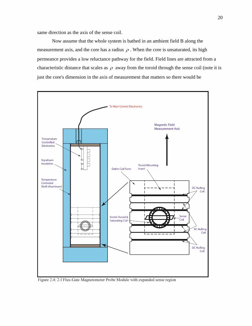
material (in our case a ferrite toroid core) with, in our case, 4 coils around it (see figure 2.4.)
The saturating coil is wrapped as a toroidal solenoid around the core. An alternating current
is put through this coil which is strong enough to magnetically saturate the core first one
way, then the other at a frequency 0f which in our case is about 500 Hz. The sense coil is
wrapped around the core in a loop whose axis points in the direction we want to measure the
field (there are actually 20 turns since totald
dt
is proportional to the number of loops) placed
in such a way that the flux change from the AC saturating field inside the toroid cancels to
zero. This is because the saturating field lines are contained in closed loops that are within
the toroid and hence cannot encircle any branch of the sense coil. The two nulling coils are
large coils (solenoid or Helmholtz-like) that produces a DC field over the whole toroid in the
20
same direction as the axis of the sense coil.
Now assume that the whole system is bathed in an ambient field B along the
measurement axis, and the core has a radius . When the core is unsaturated, its high
permeance provides a low reluctance pathway for the field. Field lines are attracted from a
characteristic distance that scales as away from the toroid through the sense coil (note it is
just the core's dimension in the axis of measurement that matters so there would be

21
advantages to having an oblong core). This increases the amount of flux going through the
sense loop. When the core is saturated, its permeance approaches that of the surrounding air.
The low reluctance path is switched off so the field in the region becomes uniform again and
the flux passing through the sense coil is reduced. For each cycle of the AC current run
through the saturating coil the core saturates first one way, then the opposite. This
component, as stated before causes no flux change in the sense coil as the current saturating
coil forms a loop thus canceling out by Ampere’s Law. When the core is unsaturated, the
extra ambient field, however, is guided through the toroid and sense loop twice each cycle
causing the flux to change with a characteristic frequency of 02 f . Thus, if there is an ambient
magnetic field, totald
dt
is non-zero and an EMF which is to first order proportional to B is
produced around the loop with a characteristic frequency 02 f or in our case about one kHz.
At this point we can servo the current going through the nulling coil to bring the 02 f
component of the signal to zero. This correction current is accurately proportional to ambient
field B.
The biggest advantage of our system over a range of copy-cat commercial units is that
the servo current going through the nulling coil can be mirrored and scaled to run through the
Helmholtz coil around the superconducting magnet. This way one does not get the extra time
delay between the ambient magnetic field changes and the system’s compensation which
comes from the pole of the magnetometer's output response, for which it is impossible to
adequately compensate (with a filter that obeys causality and doesn't do terrible things to the
noise floor). In fact, when we were initially testing the system, we found the overall
compensation factor improved significantly as we decreased the integrator time constant,
reducing filter averaging. This is a design choice that was not available with off the shelf
components since they used low pass filtering to improve the D.C. specs of the
magnetometer to the detriment of their use in a magnetic cancellation system.
There were several other important details in the system design and possible
improvements for a future system. First, the nulling coil was divided into two sections. The
first was for providing the main DC magnetic field to do most of the nulling at the probe. A
second was for providing the AC magnetic field changed that canceled out the time varying
noise. This allowed for much lower currents in the large compensating Helmholtz coil around
22
the magnet since it did not have to contain the scaled DC term. This consequently simplified
the electronics design. It also allowed for convenient, and independent control of the nulling
loop's loop gain by wrapping it with a different number of turns than the DC coil. Thus the
AC coil was not burdened with the design constraints that would be imposed had it been
required to null out the entire field. Additionally, it was important to temperature stabilize the
fluxgate probe. The dominant source of error here was the large thermal expansion
coefficient of the plastic probe housing, which was almost two orders of magnitude worse
than the fundamental limits in the electrical components used. There was also the second
order effect from the change in the core’s saturating current with temperature. Another point
to consider is that the probe housing must not be made of a continuous metal enclosure since
the eddy currents in this will low pass filter the magnetic field noise changes leading to poor
system cancellation (as in our prototype probe). And finally, the nulling coil should be much
larger than the sense toroid. This improves the linearity of the system.
Considering the ample signal our 1.25” toroid provided, a smaller core would have
been more than adequate and would have increased the frequency we could have run at for a
given power (power dissipation in the probe varies as it's volume, signal varies as 2 .)
Increasing the frequency would have improved the frequency response of the device and
compensated for the reduction of signal from decreasing . Additionally, unless the
frequency of the coil were increased by a great deal, no doubt a superior system could be
constructed with supermalloy tape wound cores. Though they are unusable past a kHz or two,
they would have a lower coercivity, less volume to saturate and a higher permeability. Also,
and more importantly, the current source that powered the DC nulling coil could have been
made at least an order of magnitude better. This will probably become necessary when mass
measurement accuracy gets in to the low part in1210 level. Note that a 2 axis magnetometer
can be made by wrapping a second pickup coil around the toroid at a 90 degree angle from
the first, and a second nulling coil on the new axis. One axis is all that was needed in this
case, and we have no indication that our magnetometer was in any way limiting us at this
level.
To give the reader some idea of what a homemade flux gate magnetometer system
can do let me speak about the magnetometer cancellation systems we made. During initial
testing, we achieved a factor of 75 cancellation of external fields. This was with a probe

23
placement about 1 meter from the magnet center. Unfortunately, the field at that point is high
enough that the long term stability of the electronics feeding the D.C. nulling coil would need
to be made an order of magnitude better. While this is possible with an LTZ1000a current
source, we decided to place the probe, instead, about 3 meters from the field center where we
got a factor of 50 cancellation. Note that it is unlikely that commercial magnetometer
systems are stable enough to be used even at the field point we used. Neither the temperature
stability of the probe, nor that of the current to voltage converter would be sufficient.
The last method that is used for reducing external magnetic noise is passive shielding.
There are two sources of passive shielding, one of which is much more important than the
other. The less important source is the shielding of the trap envelope. The conductivity of the
metallic trap envelope increases some, though not as much as a pure metal would, when it
goes down to liquid helium temperatures. By Lenz' law, the eddy currents in the envelope
resist magnetic field changes at high frequency; however, because of the good conductivity
of the metal at liquid helium temperatures, this shielding extends down reasonably low in
frequency. This is illustrated every time we lower the experiment down into the field and
when we take it back out. The process of putting in the experiment is relatively easy as the
envelope is warm. Pulling it back out of the field when it is cold, however, requires
considerable force and time (subjectively, maybe 10 lbs on a 4x block and tackle and a
couple of minutes to move 15 inches.) This high frequency shielding decreases the impact of
rapid signals that would be faster than the 2-f flux gate’s electronics.
The most important passive screening effect comes from the superconducting
solenoid itself and its inner compensation solenoid. A superconducting magnet will have a
natural shielding factor of about 5 due to the fact that flux does not pass through the
superconducting wire. To enhance this, the magnet has another superconducting solenoid of
the proper size wrapped around the central bore [27]. With the tolerances available in such
devices the shielding at its center is another factor of 35-40 better. These two effects extend
down to D.C. Note the active and passive compensation systems just eliminate external
noise, but they do not eliminate field wander from thermal effects in the bore. These must be
addressed by magnet stabilization techniques as described earlier in this section.

24
Chapter III: Derivatives of First Order Physics
In the last chapter I introduced the basic physics of the normal modes of Penning
traps in general and some aspects of the UW Penning trap in specific relating to it. The next
layer of explanation will cover the consequences of this physics while largely keeping in the
realm of the linear system. Up until now, there has been no discussion of how the frequencies
are measured. This will not be entirely answered yet since more physics needs to be
discussed first, but I will present how we interrogate the axial motion of the particle and the
noise seen on this measurement.
In principle, each of the normal modes in the trap can be measured in a non-
destructive way. The difficulty with this is that it does not allow a dissipative path to get
energy out of the particle once it is excited. In addition, such couplings would be so weak
that it would require prohibitively narrow bandwidths to overcome amplifier noise. However,
coupling the particle’s axial motion to a cryogenic thermal bath allows the particle’s motion
to be cooled and, in addition, it provides a convenient mechanism to make a measurement of
the coupled axial mode. From our measurement of the phase of this mode relative to a stable
drive frequency we can interrogate its state and infer the state of the other modes. The
measurement of the axial mode is central to the experiment and we have spent some time
refining the techniques with which we measure it. In addition to this I will discuss the
particle lock loop which keeps z exactly where we want it, and provides real time
monitoring of the experiment, along with many other desirable features.
Section III.1: Particle Damping and Driving
In this section I will discuss the driving and damping of the particle's axial motion in
the approximation that the axial motion of the particle is completely harmonic. The axial
motion of the particle is coupled to the outside world through its image currents in the trap’s
endcap electrodes. If the two endcaps were grounded conductors, the positive charge of the
ion would be attracted to the endcap it is nearest to by the negative charge it induces on the
endcaps. This slightly lessens the axial frequency of the particle, which will be discussed
later, but it does not remove any energy. However, when these image currents are run

25
through an electrical element connected between ground and one of the endcaps (called the
“signal endcap”) some of the energy in the particle’s motion is damped out.
The standard treatment is to say that a moving charge with velocity dzdt
induces a
current in the endcaps of
02
q dzK
z dt (3.1)
where K is on the order of 1 and reflects the departure of the geometry from infinite
capacitor plates. This current passes through an impedance Z which creates a voltage
02
q dzV ZI ZK
z dt (3.2)
on the endcap which in turn creates a self-interaction field at the center of the trap of
2
2
04
q dzE ZK
z dt (3.3)
and a force on the particle of
2 2
2 2
2 2
0 0
where .4 4
z z
q dz dz qf ZK m ZK
z dt dt mz
(3.4)
To be entirely correct Z is complex, and so is the damping constant. If Z is inductive
z goes down a little bit and if Z is capacitive z goes up a bit. This is a small and
irrelevant effect since it is a correction of less than a few parts in 1210 of the axial frequency,
which is a quantity that is further reduced by a factor of 2
2
z
c
in importance by the quadrature
equation 2.13. If Z has a real component, R, then this acts to damp the particle’s motion. To
quantify this, I will write down the driven equation of motion (using d
Ddt
)where I have
used the fact that E&M is linear to absorb the particle’s self-interaction into a viscous
damping term:
2 2
0
( )( ) ( ) .
2
drz z
qKV tm D D z t qE t
z (3.5)
where E(t) is the field from an applied rf drive at the center of the trap. The voltage to create
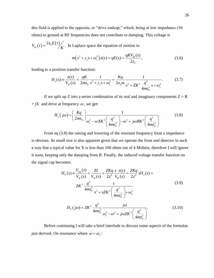
26
this field is applied to the opposite, or “drive endcap,” which, being at low impedance (50
ohms) to ground at RF frequencies does not contribute to damping. This voltage is
02dr
z E tV t
K . In Laplace space the equation of motion is:
2 2
0
( )( ) ( ) ,
2
drz z
qKV sm s s z s qE s
z (3.6)
leading to a position transfer function:
22 2
2 2 20 02
0
( ) 1 1( ) .
( ) 2 2
4
z
dr z zz
z s qK KqH s
qV s mz s s z ms ZK s
mz
(3.7)
If we split up Z into a series combination of its real and imaginary components Z = R
+ jX and drive at frequency , we get:
2 2
2 2 2 20
2 2
0 0
1.
2
4 4
z
z
KqH j
mz q qXK j RK
mz mz
(3.8)
From eq (3.8) the raising and lowering of the resonant frequency from a impedance
is obvious. Its small size is also apparent given that we operate the front end detector in such
a way that a typical value for X is less than 100 ohms out of 4 Mohms, therefore I will ignore
it soon, keeping only the damping from R. Finally, the induced voltage transfer function on
the signal cap becomes:
0 0
22
2 22 2 20
2
0
( ) ( )( ) ( )
( ) ( ) 2 ( ) 2
4
4
sig
V z
dr dr dr
z
V s ZI ZKq s z s ZKqH s sH s
V s V s z V s z
q sZK
mz qs sZK
mz
(3.9)
2
2
2 22 2 20
2
0
( ) .4
4
V
z
q jH j ZK
mz qj ZK
mz
(3.10)
Before continuing I will take a brief interlude to discuss some aspects of the formulas
just derived. On resonance where z :
27
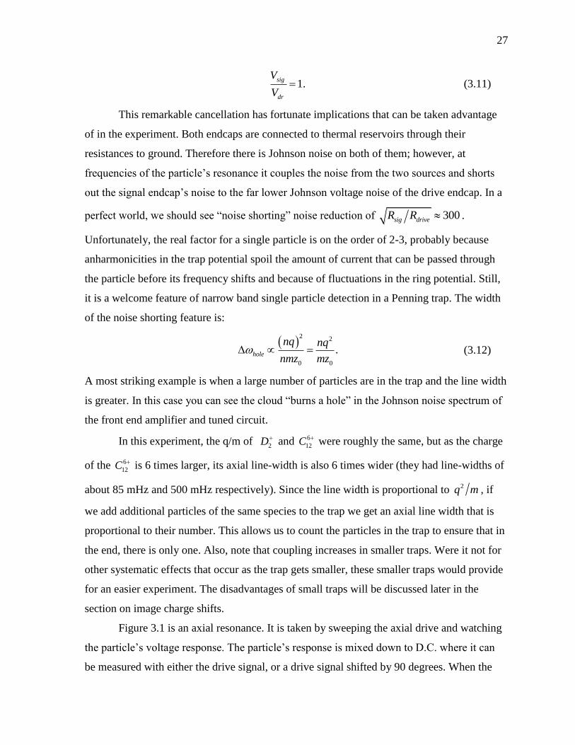
1.sig
dr
V
V (3.11)
This remarkable cancellation has fortunate implications that can be taken advantage
of in the experiment. Both endcaps are connected to thermal reservoirs through their
resistances to ground. Therefore there is Johnson noise on both of them; however, at
frequencies of the particle’s resonance it couples the noise from the two sources and shorts
out the signal endcap’s noise to the far lower Johnson voltage noise of the drive endcap. In a
perfect world, we should see “noise shorting” noise reduction of 300sig driveR R .
Unfortunately, the real factor for a single particle is on the order of 2-3, probably because
anharmonicities in the trap potential spoil the amount of current that can be passed through
the particle before its frequency shifts and because of fluctuations in the ring potential. Still,
it is a welcome feature of narrow band single particle detection in a Penning trap. The width
of the noise shorting feature is:
2 2
0 0
.hole
nq nq
nmz mz (3.12)
A most striking example is when a large number of particles are in the trap and the line width
is greater. In this case you can see the cloud “burns a hole” in the Johnson noise spectrum of
the front end amplifier and tuned circuit.
In this experiment, the q/m of 2D and 6
12C were roughly the same, but as the charge
of the 6
12C is 6 times larger, its axial line-width is also 6 times wider (they had line-widths of
about 85 mHz and 500 mHz respectively). Since the line width is proportional to 2q m , if
we add additional particles of the same species to the trap we get an axial line width that is
proportional to their number. This allows us to count the particles in the trap to ensure that in
the end, there is only one. Also, note that coupling increases in smaller traps. Were it not for
other systematic effects that occur as the trap gets smaller, these smaller traps would provide
for an easier experiment. The disadvantages of small traps will be discussed later in the
section on image charge shifts.
Figure 3.1 is an axial resonance. It is taken by sweeping the axial drive and watching
the particle’s voltage response. The particle’s response is mixed down to D.C. where it can
be measured with either the drive signal, or a drive signal shifted by 90 degrees. When the
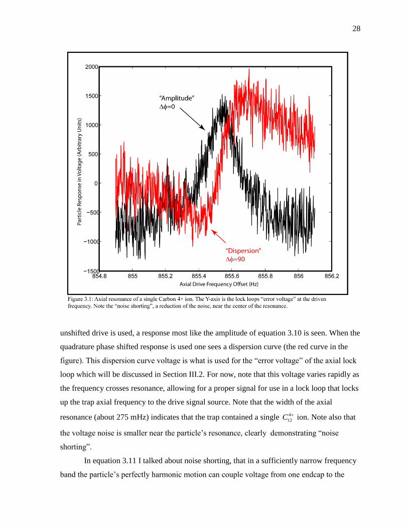
28
unshifted drive is used, a response most like the amplitude of equation 3.10 is seen. When the
quadrature phase shifted response is used one sees a dispersion curve (the red curve in the
figure). This dispersion curve voltage is what is used for the “error voltage” of the axial lock
loop which will be discussed in Section III.2. For now, note that this voltage varies rapidly as
the frequency crosses resonance, allowing for a proper signal for use in a lock loop that locks
up the trap axial frequency to the drive signal source. Note that the width of the axial
resonance (about 275 mHz) indicates that the trap contained a single 4
12C ion. Note also that
the voltage noise is smaller near the particle’s resonance, clearly demonstrating “noise
shorting”.
In equation 3.11 I talked about noise shorting, that in a sufficiently narrow frequency
band the particle’s perfectly harmonic motion can couple voltage from one endcap to the

29
other. It could be argued that this is a rather circuitous way to get the voltage across the trap.
What about the much simpler and broader band direct capacitive coupling? Why wouldn’t
this swamp out, the signal of the particle’s motion? In fact, at one point in the past this was a
major concern and a system was devised to cancel out the drive feed through with a tuned
transformer. Soon, however, a much more elegant solution was devised.
By modulating the potential on the ring electrode, in this case at 100 kHz, a sideband
parametric excitation is opened for the particle’s axial motion 100 kHz above and below the
normal mode frequency of the particle. Except for an overall increase in the amount of RF
drive required to excite the motion to a given amplitude, there is no difference between
driving on the sideband and driving directly on the resonance. With the advantage being that
this moves the feed-through signal far off the sensitivity band of the front end amplifier. For
a more complete discussion of this see the references [25]. Noting the increased axial drive
necessary, in the remainder of this work I will, therefore, ignore the ring modulation and
endcap-to-endcap capacitive feed-through entirely.
As stated earlier in this section, the particle’s motion induces a current in the signal
endcap proportional to its velocity. A design goal of the spectrometer is to detect this 3.55
MHz current with as little added noise as possible. Current multiplier devices like bipolar
transistors tend to have front end current shot noise that would compete with particle’s
signal. Several active circuits can be used to generate resistive power absorption with noise
below that of a resistor, but only at reasonably low input impedances – they are much more
suited to impedance matching of transmission lines. Therefore high input impedance voltage
input FET devices are a good choice for the front end preamplifier.
Having a Z which is pure capacitance or inductance would be an ideal situation since
they have no Johnson noise. However, since there is at least 12 pF to ground of stray parallel
capacitance to the signal endcap, the magnitude of the impedance is too low to generate
much voltage for a signal. In addition, there would not be anything to get energy out of the
particle’s motion. The best solution is to cancel the stray capacitance at the input frequency
with an inductor to form a “tank” circuit. To first order a tank circuit can be characterized by
its center frequency and its “Q” or quality factor which is the reciprocal of the fractional
energy lost per cycle. The resistance on resonance is the Q times the reactance of either the
capacitance or the inductor. The lower the parasitic losses in the reactive elements are, the

30
lower the conductance at resonance and the higher the parallel resistance.
The Johnson current noise of a resistor is:
2 24 n
kTi amp
R (3.13)
where is the observation bandwidth. In order to have the highest signal to noise ratio we
need to get ni as low as possible. In order to do this we need to lower the temperature (we
use 4.2K liquid helium) and raise the resistance. Our cryogenic tank circuit is a helical
resonator which is a self-shielding heavily loaded quarter wave resonator. This along with the
stray 12 pF of capacitance makes a parallel tuned circuit with a Q of 1300 at cryogenic
temperatures. On resonance this behaves like a resistor of about 3.5 M for an
8noise
fAi
Hz .
Now I will proceed with the derivations. Next we will look at the phase of the
detected signal relative to the drive. This can be derived easily from its signal transfer
function. Since we usually operate on the resonance of the tank circuit (it is much wider than
the particle resonance), I will treat tankZ as a pure resistance and R and z as real.
2 2
1
2 2tan z
V
z z z
jArg H j Arg
j
(3.14)
when Taylor expanded with z this becomes:
1 2
tanz
(3.15)
or, for small phi, the phase is equal to twice the negative of the fraction of full line widths
from resonance. Thus the phase of the signal relative to the drive is a measure of the error
from the potential well’s natural frequency. This becomes important because if we are
detecting the particle by mixing in the wrong phase, the true axial frequency is different from
the number that is dialed up on the RF frequency synthesizer. Our ability to measure this
phase accurately is the current limiting systematic on the accuracy of the spectrometer.
Section III.2: Detection System, Lock Loop, Signal Chain Electronics
As stated earlier, we detect the particle’s axial motion. We use this information in a

31
feedback system to stabilize the voltage of the Penning trap’s ring electrode. In turn, the
parameters of this lock loop tell us things about the state of the particle. This section includes
the implementation of the feedback system and the loop equations governing it. Since this
section is dealing with the signal chain, at least that section of the electronics will be
discussed here.
Figure 3.2 is a simplified diagram that emphasizes the frequency lock loop and the
ring voltage system – among other things the ring modulation has been left out, two of the
intermediate frequencies (IF) and most of the frequency mixes/synthesis have been
simplified, but the components needed for computation remain. The endcaps are kept at DC
ground and, as discussed last chapter, the particle oscillates at a frequency determined by the
voltage difference between the endcaps and potential placed on the ring electrode.
32
The image charge currents of the particle’s motion induce a voltage on the tank
circuit. This voltage is detected by a pair of cryogenic GaAs FETs in a cascode configuration
which multiply the particle’s motional currents by about510 . Ignoring cable tuning which
gives another factor of a few, this composite first stage coming out the cryogenic
environment gives about 45 dB of power gain – a comfortable margin above the roughly
20dB needed to lift the signal out of the relatively larger Johnson noise of the room
temperature electronics.
In the experiment, gain is spread out over four frequencies including D.C. with the
local oscillator (LO) for each mix stage synthesized in a way to carefully preserve the phase
of the particle in the face of inevitable phase wander of the frequency sources; this will be
covered in more detail in chapter 6. In the simplified model, all of this gain is at 3.5 MHz and
the AC signal is down-converted to DC by mixing with the drive signal phase shifted by 90
degrees. This is the frequency lock loop’s frequency “error signal,” or the error in phase from
the drive times the axial drive amplitude. It is then passed through a loop filter, in this case,
an integrator, to form the “correction signal”. The correction signal is divided down and
added to the negative voltage on the ring by bootstrapping the positive end of the reference
batteries. Thus the voltage on the ring is stabilized and brought up to the value needed to
make the trapped particle’s axial resonant frequency the same as the drive frequency.
The energy in the particle’s driven motion is on the order of 5 times the thermal
energy at 4.2K; this comes out to about 223 10 J or 2 meV. This energy is extracted at the
rate of the particle’s line width for a total received power of around 100 yoctowatts or -190
dBm. This must be amplified to the milliwatt range so that it can be dealt with comfortably
by digitizing electronics. If all this gain were at broad band, the final signal would have a
power of several kilowatts. This broadcasting station would unnecessarily complicate the
experimental design and put ridiculous requirements on the linearity of the analog to digital
converter in the inevitable computer, not to mention using needless digital signal processor
time. In the spirit of not preserving irrelevant information (remember that no information
comes out of the particle faster than the rate determined by its axial line-width – 500 mHz for
6
12C and 85 mHz for 2D ) we limit the bandwidth of the electronics as much as is practical.
We also place as much gain as possible at “high” frequencies which are away from the 1/f
noise limitations of easily available electronics and D.C. wanders which would show up as

33
phase inaccuracy in the phase systematic.
One of the chief purposes of the loop is to bandwidth limit the signal coming from the
front end. As such, it is useful to look at the loop transfer functions. As seen in figure 3.2, the
band-pass nature of the particle’s line-width and the detection bandwidth of the system can
be turned into a low-pass filter response when the signal is mixed down to D.C. The voltage
on the ring becomes a voltage to frequency converter for the particle. An integrator is used to
complete the loop filter and insures that the D.C. phase error of the loop is zero. Please note
that this is a “frequency-lock loop” and not a “phase-lock loop”. In a phase lock loop the
particle’s phase error could integrate off to infinity if there were an error in frequency. Here,
a constant frequency error is turned into a constant phase error, the phase between the
particle’s natural motion and the signal that drives it which can vary from to .2 2
As
there is no natural integration of the particle’s phase, the loop is of the frequency-lock type.
As the phase difference, which is proportional to the frequency difference for small angles, is
measured, the technique is called “phase sensitive detection”.
Figure 3.2 shows a base-band model for the feedback loop. A frequency change that
arises from a change in the environment of the particle is amplified and integrated, then fed
back on to the ring voltage line to correct the voltage on the trap so that the natural frequency
of the particle comes back to the drive frequency. The transfer function for the correction
signal takes the following form:
2
1 2
3 2 2
1 2 1 2
.
22
Drive cf zcorrection
cf z
cr z Drive cf z
A A A BVs
fs s s A A A BC C
(3.16)
Here, the crystal filter’s width is 52
cfHz
, the particle’s line-width is
2
z
, and the other
constants defined as shown in figure 3.2. Because the crystal filter is considerably faster than
the rest of the loop dynamics, its transfer function can be approximated as 1 (insertion loss is
being absorbed elsewhere) to give an approximate transfer function of:
2
2 2
.
2
correction z
zz
V ABs
fs s ABC
(3.17)

34
Here the A’s and C’s have been contracted as 1 2 DriveA A A A and 1 2C C C .
The C coefficients are easily calculated, but the exact size of the A coefficients are
dependent on a very small drive voltage at the drive endcap, the strength and frequency of
the ring modulation, and exact gains and insertion losses of the various amplifiers. Rather
than estimate these, it is better to measure them. This can be done by breaking the loop at the
“error signal” (see figure 3.3). Next you put in an input ramp that is slow enough to not
engage the low pass response of the particle at the “correction voltage” port, then watch the
“error signal”. Because the D.C. transfer function of the error signal is:
1 2 1 2 1 2 1 2
0
2 2 20
1 12 2
error Drive Drive
correction z z
z
z cfs
V A A A C C A A A C C AC
V s s
(3.18)
the slope of the resultant line, along with the calculated C’s and measured z give a value for
35
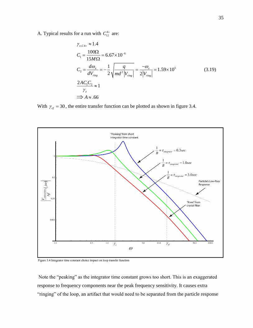
A. Typical results for a run with 4
12C are:
, 4
6
1
5
2 2
1 2
1.4
1006.67 10
15
11.59 10
2 2
21
.66
z C
z z
ring ring ring
z
CM
d qC
dV md V V
AC C
A
(3.19)
With 30cf , the entire transfer function can be plotted as shown in figure 3.4.
Note the “peaking” as the integrator time constant grows too short. This is an exaggerated
response to frequency components near the peak frequency sensitivity. It causes extra
“ringing” of the loop, an artifact that would need to be separated from the particle response

36
(the upsweep of which has a “ringing” of its own which is not an artifact). This comes from
trying to push the loop time constant faster than the axial line-width of the particle. To a
limited extent, this peaking can be compensated for, but since no information is coming out
of the particle at this rate, this accentuates electronic noise.
A great deal more freedom exists than one might expect as long as the integrator time
constant is long enough. There really is not much that is fast for the loop to respond to except
for electronics noise. For this reason the sweep fits are often more reliable with longer
integrator time constants. It can also be seen in the figure that the crystal filter’s impact on
the dynamics falls far outside the stop-band for the loop. This is not to imply that it is
irrelevant to the experiment. Noise that goes through its pass band makes a real impact on the
experiment and the gain “A” can be turned up with a narrower filter. The crystal filter is
designed to have as narrow a band-width as possible. In fact, after the deuterium work was
completed, a newer filter with half the bandwidth was designed and fabricated for the 3He
work.
Long integrator time constants do have some cost, however. By looking at the
response of equation 3.17 to a ramp input (noting that 2
1L t u t
s for those unfamiliar
with Laplace transforms), then taking the two lowest frequency terms (we are going to take
the long time limit):
2
low freq
, 22 32 2
1 1.
1
22
zcor ramp
zz
z
ABV s
sCs ss s ABC
AB
(3.20)
Next take the inverse Laplace transform of this to get the time response and take the limit as t
gets large:
2 t large1
2 3
1 1 1 1 11 .
1 2 2
2
zABC
z z
z
L e t tC ABC C ABC
Cs sAB
(3.21)
This is clearly the D.C. loop gain, 1
C, times a ramp function delayed by a time
1
2 zABCor
the effective first order loop time constant which, in our case of 4
12C , equals 1.6 seconds. This

37
is important because our up and down sweeps have ramp responses in them. For a 5 minute
sweep over 50 mHz, this is about 0.27 mHz shift (~6 ppt). Since the up sweep and down
sweep have the same time lag in different frequency directions, the two shifts average to 0.
This will be illustrated and discussed further in chapter 4 in the section on sweep response.
Section III.3: Front End Noise
I will start this section by describing the front end electronics of the tuned
circuit/preamplifier and use this to launch a discussion of the noise that the front end of the
experiment sees. This noise has different sources, all of which do not impact the experiment
in the same way. Some considerable effort goes into making the front end tuned circuit and
amplifier in various Penning trap experiments. This subject is not often part of the
preparation of a typical experimental physicist. The conditions found in these types of
experiments are significantly different from the usual ones found in typical electrical
engineering problems, though they are more thoroughly discussed in that context, and,
ironically, they share some of the same concerns of those multi-gigahertz circuits. Since I had
spent some time bringing myself up to speed on the subject and have seen other groups with
questions on the topic, I will discuss it in a little more depth.
The front end tuned circuit creates a high impedance point at the signal endcap. This
high impedance point changes the extremely high impedance current source of the particle
into a voltage signal that can be detected by a parametric amplifier (a field effect transistor,
or FET, is a type of parametric amplifier as you are varying a parameter of the amplifier, its
gate voltage, to modulate its channel current). It is hopeless to attempt to match the particle’s
impedance to the high impedance point because that is far too high given the 710 “Q” of the
particle’s motion. We have used a self-shielding tank circuit called a “helical resonator” to
generate an RF impedance of almost 4 megaohms. A diagram of the resonator is shown in
figure 3.5. The self-shielding and compact nature of the resonator prevents it from becoming
microphonic as initial attempts at resonator design were. The resonator is also immersed in
liquid helium to limit Johnson noise currents that would warm up the particle’s motion and
provide extra detector noise.
To continue on a lighter note, as anyone who has tried to construct an amplifier for

38
this type of experiment knows, in spite of great efforts to eliminate it, feedback is
unavoidable and as the old Murphy’s Law adage goes, “amplifiers oscillate, oscillators
don’t.” If you have done your work carefully enough usually the circuit won’t oscillate at the
resonant frequency of tank circuit. This is a very good thing, because any oscillation at that
frequency strongly couples to the particle’s resonant axial motion and often throws it out of
the trap. To see a way (and certainly not the only way) this could happen, look at the
simplified front ends in fig. 3.6, which illustrate what can happen if insufficient care is taken
in assembling the trap and preamplifier assemblies.
Note that stray inductance between the source of the FET and ground will couple to
some extent with the very high impedance of the helical resonator. This can create a circuit

39
that looks suspiciously like a common drain transformer coupled oscillator. And, if the pre-
amp output cable couples to the helical resonator, a common source transformer coupled
oscillator is formed. The standard criterion for oscillation is for the energy coupled back into
the tank circuit (helical resonator) from the amplifier to exceed the losses in the tank. The
cryogenic helical resonator has a “Q” of 1200-1500 and thus provides very little loss for the
amplifier and coupling to overcome. At these frequencies and at cryogenic temperatures, the
amplifier FET provides on the order of 50 dB of power gain so a small amount of coupling
can easily be enough for an oscillation to start. The frequency of this oscillation would be
near the peak frequency of the tank which is also chosen to be the natural frequency of the
particle. Pumping the particle with a volt or larger size signal near its resonance is more than
40
enough to throw the particle into the endcaps where it is lost. Note that the back-to-back
diodes shown in figure 3.4 limit oscillation size to some extent, but are insufficient to stop a
determined oscillator from kicking the particle of interest out of the trap.
There are amplifier problems other than tuned circuit coupling. Usually, the designer
buys a device and expects it to behave as its specifications indicate in the application. The
physicist, however, has anything but typical problems. When cooling a GaAs device to 4.2K,
as hinted at in the last paragraph, its transconductance goes up an unpredictable amount as
phonon-carrier scattering drops away and defect-carrier scattering takes over (in HEMTs,
usually the channel is a layer doped neutrally so dopant-carrier scattering is also suppressed,
exacerbating the problem.) This frequently causes the device itself to form an oscillator and
an overvoltage condition which can degrade or destroy the device. With the process
transition frequencies 300Tf GHz at room temperatures possibly going up past 1THz at
4.2K, there is little one can do to stabilize such a device save designing the circuit board
defensively and starving the current to limit the available gain.
The one advantage we have is that the high frequency parasitic resonators have
components that have characteristic impedances near the vacuum impedance of 377 ohms
modified by the dialectric constant of GaAs or circuit board materials. Therefore they can be
snubbed with small resistors placed judiciously near the FET. Since voltage noise of a 33
ohm resistor is much less than the front-end detector’s impedance this can be done without a
significant degradation of the circuit’s noise figure. A note: maximal damping would be with
resistors in the 50-100 ohm vicinity since this would individually terminate each of the wires
coming from the FET.
Though it can cause oscillation, feedback is not all bad. In practice, a small
amount of feedback is often injected back in the circuit in order to change the front end
impedance (traditionally called regeneration or degeneration depending on the sign, but also
found in the physics literature as electronic heating/cooling because it changes the effective
temperature of the tank). To see its effects on gain, look at figure 3.7.
; .1
in eff m
RZ R A G R
A
(3.22)
The onset of oscillation, and something to be avoided, is evident as A approaches 1. Note
here that Gm is not the transconductance of the FET, but the transconductance of the

41
feedback by whatever path it chooses. Raising or lowering of the front end impedance this
way is very useful since it changes the particle’s damping and axial line-width, but it does
not come without a cost. If we add basic noise sources:
2 2
, , 2 2 2
, , , ,
v v 1v v v v .
1 1 1
n front n amp
n total n total n front n amp
A A
A A A
(3.23)
(The approximation in the second equation comes from the assumption that the front end
noise and the amplifier voltage noise are uncorrelated. It is well known that this is not true,
see Van Der Ziel [28], but in this case it matters little and we can ignore it anyway.) We use
only moderate feedback since high levels of it can cause the phase delay in the amplifier
chain to vary more [by a factor 1/(1-A)] with FET aging and bias conditions. This makes the
amplifier contribution to the noise power (proportional to 2v ) small compared to the other
noises in the system since:
2 2
2 2
,
,
4 2(v 4 ) (v ) ; 3.
3n front TC TC FET
m FET
volt kT voltkT R
Hz g Hz
(3.24)
Under this approximation, an effective temperature of the front end can be defined from the
amount of noise seen on the tuned circuit and its effective resistance:
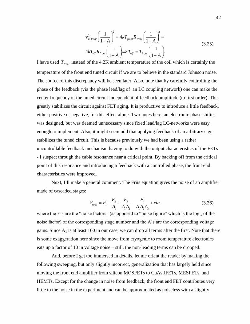
42
2 2
2
,
1 1v 4
1 1
1 14 .
1 1
n front front front
eff front eff front
kT RA A
kT R T TA A
(3.25)
I have used frontT instead of the 4.2K ambient temperature of the coil which is certainly the
temperature of the front end tuned circuit if we are to believe in the standard Johnson noise.
The source of this discrepancy will be seen later. Also, note that by carefully controlling the
phase of the feedback (via the phase lead/lag of an LC coupling network) one can make the
center frequency of the tuned circuit independent of feedback amplitude (to first order). This
greatly stabilizes the circuit against FET aging. It is productive to introduce a little feedback,
either positive or negative, for this effect alone. Two notes here, an electronic phase shifter
was designed, but was deemed unnecessary since fixed lead/lag LC-networks were easy
enough to implement. Also, it might seem odd that applying feedback of an arbitrary sign
stabilizes the tuned circuit. This is because previously we had been using a rather
uncontrollable feedback mechanism having to do with the output characteristics of the FETs
- I suspect through the cable resonance near a critical point. By backing off from the critical
point of this resonance and introducing a feedback with a controlled phase, the front end
characteristics were improved.
Next, I’ll make a general comment. The Friis equation gives the noise of an amplifier
made of cascaded stages:
32 4total 1
1 1 2 1 2 3
F .FF F
F etcA A A A A A
(3.26)
where the F’s are the “noise factors” (as opposed to “noise figure” which is the log10 of the
noise factor) of the corresponding stage number and the A’s are the corresponding voltage
gains. Since A1 is at least 100 in our case, we can drop all terms after the first. Note that there
is some exaggeration here since the move from cryogenic to room temperature electronics
eats up a factor of 10 in voltage noise – still, the non-leading terms can be dropped.
And, before I get too immersed in details, let me orient the reader by making the
following sweeping, but only slightly incorrect, generalization that has largely held since
moving the front end amplifier from silicon MOSFETs to GaAs JFETs, MESFETs, and
HEMTs. Except for the change in noise from feedback, the front end FET contributes very
little to the noise in the experiment and can be approximated as noiseless with a slightly
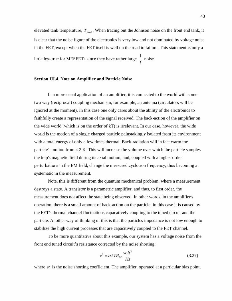
43
elevated tank temperature, frontT . When tracing out the Johnson noise on the front end tank, it
is clear that the noise figure of the electronics is very low and not dominated by voltage noise
in the FET, except when the FET itself is well on the road to failure. This statement is only a
little less true for MESFETs since they have rather large 1
f noise.
Section III.4. Note on Amplifier and Particle Noise
In a more usual application of an amplifier, it is connected to the world with some
two way (reciprocal) coupling mechanism, for example, an antenna (circulators will be
ignored at the moment). In this case one only cares about the ability of the electronics to
faithfully create a representation of the signal received. The back-action of the amplifier on
the wide world (which is on the order of kT) is irrelevant. In our case, however, the wide
world is the motion of a single charged particle painstakingly isolated from its environment
with a total energy of only a few times thermal. Back-radiation will in fact warm the
particle's motion from 4.2 K. This will increase the volume over which the particle samples
the trap's magnetic field during its axial motion, and, coupled with a higher order
perturbations in the EM field, change the measured cyclotron frequency, thus becoming a
systematic in the measurement.
Note, this is different from the quantum mechanical problem, where a measurement
destroys a state. A transistor is a parametric amplifier, and thus, to first order, the
measurement does not affect the state being observed. In other words, in the amplifier's
operation, there is a small amount of back-action on the particle; in this case it is caused by
the FET's thermal channel fluctuations capacatively coupling to the tuned circuit and the
particle. Another way of thinking of this is that the particles impedance is not low enough to
stabilize the high current processes that are capacitively coupled to the FET channel.
To be more quantitative about this example, our system has a voltage noise from the
front end tuned circuit’s resistance corrected by the noise shorting:
2
2v TC
voltkTR
Hz (3.27)
where is the noise shorting coefficient. The amplifier, operated at a particular bias point,
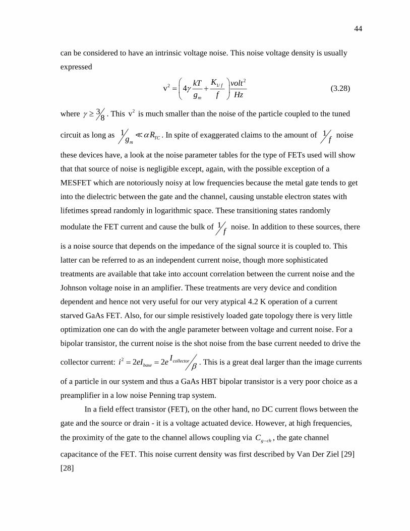
44
can be considered to have an intrinsic voltage noise. This noise voltage density is usually
expressed
2
1/2v 4f
m
KkT volt
g f Hz
(3.28)
where 38
. This 2v is much smaller than the noise of the particle coupled to the tuned
circuit as long as 1TC
m
Rg
. In spite of exaggerated claims to the amount of 1f
noise
these devices have, a look at the noise parameter tables for the type of FETs used will show
that that source of noise is negligible except, again, with the possible exception of a
MESFET which are notoriously noisy at low frequencies because the metal gate tends to get
into the dielectric between the gate and the channel, causing unstable electron states with
lifetimes spread randomly in logarithmic space. These transitioning states randomly
modulate the FET current and cause the bulk of 1f
noise. In addition to these sources, there
is a noise source that depends on the impedance of the signal source it is coupled to. This
latter can be referred to as an independent current noise, though more sophisticated
treatments are available that take into account correlation between the current noise and the
Johnson voltage noise in an amplifier. These treatments are very device and condition
dependent and hence not very useful for our very atypical 4.2 K operation of a current
starved GaAs FET. Also, for our simple resistively loaded gate topology there is very little
optimization one can do with the angle parameter between voltage and current noise. For a
bipolar transistor, the current noise is the shot noise from the base current needed to drive the
collector current: 2 2 2 collector
base
Ii eI e
. This is a great deal larger than the image currents
of a particle in our system and thus a GaAs HBT bipolar transistor is a very poor choice as a
preamplifier in a low noise Penning trap system.
In a field effect transistor (FET), on the other hand, no DC current flows between the
gate and the source or drain - it is a voltage actuated device. However, at high frequencies,
the proximity of the gate to the channel allows coupling via g chC , the gate channel
capacitance of the FET. This noise current density was first described by Van Der Ziel [29]
[28]
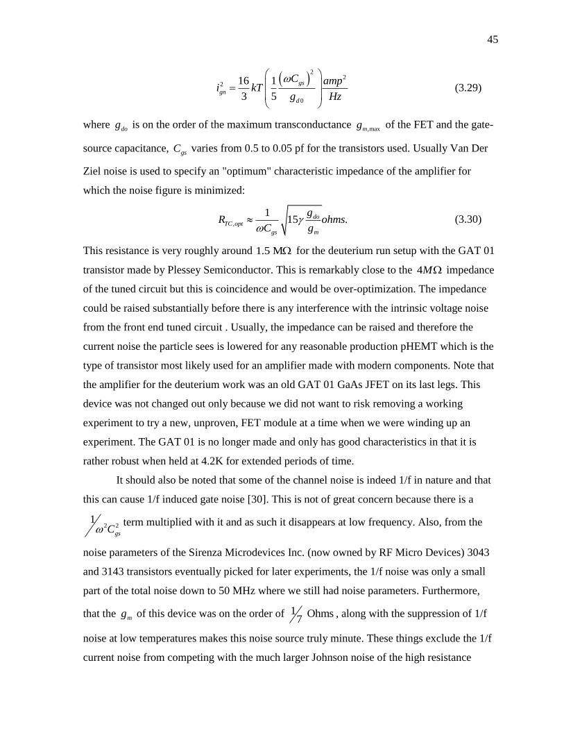
45
22
2
0
16 1
3 5
gs
gn
d
C ampi kT
g Hz
(3.29)
where dog is on the order of the maximum transconductance ,maxmg of the FET and the gate-
source capacitance, gsC varies from 0.5 to 0.05 pf for the transistors used. Usually Van Der
Ziel noise is used to specify an "optimum" characteristic impedance of the amplifier for
which the noise figure is minimized:
,
115 .do
TC opt
gs m
gR ohms
C g
(3.30)
This resistance is very roughly around 1.5 M for the deuterium run setup with the GAT 01
transistor made by Plessey Semiconductor. This is remarkably close to the 4M impedance
of the tuned circuit but this is coincidence and would be over-optimization. The impedance
could be raised substantially before there is any interference with the intrinsic voltage noise
from the front end tuned circuit . Usually, the impedance can be raised and therefore the
current noise the particle sees is lowered for any reasonable production pHEMT which is the
type of transistor most likely used for an amplifier made with modern components. Note that
the amplifier for the deuterium work was an old GAT 01 GaAs JFET on its last legs. This
device was not changed out only because we did not want to risk removing a working
experiment to try a new, unproven, FET module at a time when we were winding up an
experiment. The GAT 01 is no longer made and only has good characteristics in that it is
rather robust when held at 4.2K for extended periods of time.
It should also be noted that some of the channel noise is indeed 1/f in nature and that
this can cause 1/f induced gate noise [30]. This is not of great concern because there is a
2 21
gsCterm multiplied with it and as such it disappears at low frequency. Also, from the
noise parameters of the Sirenza Microdevices Inc. (now owned by RF Micro Devices) 3043
and 3143 transistors eventually picked for later experiments, the 1/f noise was only a small
part of the total noise down to 50 MHz where we still had noise parameters. Furthermore,
that the mg of this device was on the order of 1 Ohms7
, along with the suppression of 1/f
noise at low temperatures makes this noise source truly minute. These things exclude the 1/f
current noise from competing with the much larger Johnson noise of the high resistance
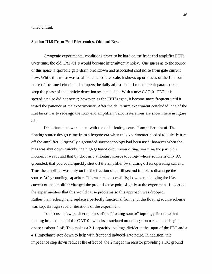
46
tuned circuit.
Section III.5 Front End Electronics, Old and New
Cryogenic experimental conditions prove to be hard on the front end amplifier FETs.
Over time, the old GAT-01’s would become intermittently noisy. One guess as to the source
of this noise is sporadic gate-drain breakdown and associated shot noise from gate current
flow. While this noise was small on an absolute scale, it shows up on traces of the Johnson
noise of the tuned circuit and hampers the daily adjustment of tuned circuit parameters to
keep the phase of the particle detection system stable. With a new GAT-01 FET, this
sporadic noise did not occur; however, as the FET’s aged, it became more frequent until it
tested the patience of the experimenter. After the deuterium experiment concluded, one of the
first tasks was to redesign the front end amplifier. Various iterations are shown here in figure
3.8.
Deuterium data were taken with the old “floating source” amplifier circuit. The
floating source design came from a bygone era when the experimenter needed to quickly turn
off the amplifier. Originally a grounded source topology had been used; however when the
bias was shut down quickly, the high Q tuned circuit would ring, warming the particle’s
motion. It was found that by choosing a floating source topology whose source is only AC
grounded, that you could quickly shut off the amplifier by shutting off its operating current.
Thus the amplifier was only on for the fraction of a millisecond it took to discharge the
source AC-grounding capacitor. This worked successfully; however, changing the bias
current of the amplifier changed the ground sense point slightly at the experiment. It worried
the experimenters that this would cause problems so this approach was dropped.
Rather than redesign and replace a perfectly functional front end, the floating source scheme
was kept through several iterations of the experiment.
To discuss a few pertinent points of the “floating source” topology first note that
looking into the gate of the GAT-01 with its associated mounting structure and packaging,
one sees about 3 pF. This makes a 2:1 capacitive voltage divider at the input of the FET and a
4:1 impedance step down to help with front end induced-gate noise. In addition, this
impedance step down reduces the effect of the 2 megaohm resistor providing a DC ground
47
48
for the gate which would otherwise limit the Q of the front end. Also note that the 1 uF
source bypass capacitor is not simply a capacitor at all frequencies. In fact, it is impossible to
produce an unadulterated 1 uF at the highest frequencies at which the FET has gain (perhaps
50 GHz at cryogenic temperatures for this old FET.) As mentioned before, stray inductuance
in the lead to this device not only degenerated the device (this part is beneficial), but provides
coupling to other parts of the circuit (not beneficial). Since the lead length is longer, this
topology is more prone to oscillation by the aforementioned parasitic elements. Due to lack
of drawing space, the transient suppression elements on the gate of the lower FET and the
drain of the grounded gate FET have been left out. These were placed as close to the GAT-01
components as was reasonable. Note however, that because these were leaded devices placed
in sockets, this distance was no closer than 1/3 inch from the device itself. This extra space is
particularly egregious at the highest frequencies the FET has gain.
After the deuterium work we had the opportunity to rebuild the front end so we could
change over from the Plessey GAT-01 transistors (nearly the first mass-market GaAs JFET
used at the advent of cable TV) and the floating source topology to a grounded source circuit
with modern pHEMTs. (A pHEMT, or MODFET, is a FET that takes advantage of the
junction between dissimilar semiconductors to produce a channel.) The first iteration of the
design is shown in the top right in figure 3.8. We got rid of the capacitive step down as this
was much less reliable with the new surface mounted devices which had input capacitances
on the order of .1 pF – this is shown in the choice of a 17 pF AC coupling capacitor. Also,
since surface mounted modules were now used, parasitic snubbing components could be
placed within 1 mm of the device itself (a factor of ten closer). In the lower, or G0 for gate
number 0, FET of this design a 2 pF capacitor was placed from source to drain in order to
decrease high frequency gain of the device. At 100 GHz, this was a 1 ohm shunt between the
two ports, but at 3.55 MHz it was 20 K which was shorted out by the source of the next FET
in the cascode chain (the G1 FET, which is upper in the figure, but below a second cascode
transistor in the room temperature electronics). The source of the FET was degenerated by a
3 ohm resistor to limit its transconductance to 1/3 mhos when the devices gain climbs at 4.2
K. Also, a 15 ohm snubber was placed at the gate – this time butted up against the device so
that there was no room to make a 4 resonant section here.

49
The common gate FET of the cascode was AC-grounded off the module in the same
way as the old floating source design with a transient suppression resistor on its drain. Note
that the voltage at the gate of the G1 FET could be changed in the old design which would
affect the source-drain in the G0 FET. This would change the drain-gate miller capacitance
in the G0 FET and change the Q of the tuned circuit by altering the feedback mechanism.
This new design with the modern FETs was much less prone to this flaw (or feature,
depending on your perspective, as it provided electronic cooling of the tuned circuit). Also to
be noted was the choice of different FETs in the G0 and G1 positions. This was because the
Sirenza 3043 had adequate 1/f noise and a lower gate to source capacitance (at the cost of
lower gain) than that of the 3143 device. As gain increases at 4.2 K, gain was never a
problem, but the reduced induced-gate noise of the device with the narrower channel (3043)
was beneficial. It should be noted for future designs that the use of a very fast device with a
narrower channel width would probably have adequate 1/f noise and yet have reduced
induced-gate noise to act back on the particle. The risk of this choice is that these devices
would be harder to stabilize with transient snubbing resistors and capacitors because of the
higher frequencies involved.
Once the grounded source design was working, we made two improved FET module
configurations that are shown at the bottom of figure 3.8. Configuration A improved upon the
standard grounded source circuit by attaching a second cascode FET butted up next to the
front end amplifier FET with the gate grounded to the case. This eliminated any stray
inductance between the two gates of the cascode and was the most stable of the variants.
Because we did not maintain a good ground plane to the gate of the second FET there is still
some chance of configuration based high impedance points (a 4
section of conductor that is
shorted at one end becomes a transmission line high impedance at the other end), but the
chances are greatly reduced. This comes at the expense of circuit linearity since there is not
much “head room” for the bottom FET to act. This is not a problem with our experiment,
however, since the signal we are detecting is on the order of 5 times thermal and there is very
little voltage gain in the preamplifier, only power gain from changing the impedance from 4
megaohms to 7 ohms. Note that feeding a 50 ohm line with a transconductor with a
1 siemens
7mg does give some voltage gain. This configuration also had on the module an
50
AC ground to the case lead in FET G1. If you are wondering why the capacitor values are as
small as they are for AC grounding purposes, it was because, at the time, larger values of
surface mount capacitor were unavailable. The standard ferroelectric dielectrics that produce
commonplace capacitors at room temperature go below their ferroelectric transition
temperature when put in liquid helium. This requires the use of multi-layer or plastic film
capacitors for all cryogenic applications. Plastic film surface mount capacitors were not
available at the beginning of this exercise.
The final FET module improvement was Configuration B. This used the same
configuration as A for the bottom FET, but has another gain stage in FET G1 for an extra 30
dB of low noise, cryogenic gain. Again, this is at the expense of linearity, but since the
signals we are detecting are very small, this does not become a problem. This was all done
with roughly the same voltage overhead and therefore the same cryogenic power dissipation.
This configuration was operated with 2V and 0.5 mA of current for a power dissipation of 1
mW and provided almost excessive gain – allowing us to turn down the room temperature IF
amplifier gain stage to near minimum. It should be noted that, as might be expected from the
high impedence G1 FET gate, this configuration was a bit more squirrelly in operation, but
still better than the original floating source circuit.

51
Chapter IV: Higher Order Physics and Implications
This Chapter discusses the non-linear physics of the experiment plus ion interactions
and ion loading.
Section 4.1: Coupling to the Cyclotron Mode
Up until this point I have only discussed how the axial mode is measured. In order to
measure the free space cyclotron frequency all the modes need to be measured per the
quadrature relation, equation 2.13. In fact, the axial mode is not even the most important one
for this measurement as can be seen in equations 2.14 and 2.15. Next I will discuss how the
trap cyclotron mode radius can be monitored continuously in a non-destructive manner.
Since the axial motion is the only mode we can directly monitor in our Penning trap,
it is necessary to couple the cyclotron mode to the axial mode in order to measure it. There
are two types of anharmonicity which can be introduced to accomplish this. The first to be
used historically was magnetic coupling, the so called “magnetic bottle,” or 2 ,B term. It is
the one that is most useful on light ions like deuterium (or electrons for a spin measurement
since it couples to the magnetic moment of the ion, intrinsic or otherwise.) It’s cost is larger
perturbations to the magnetic trap modes through the average residual energies left in each
mode by the centering process. The second coupling is electrical, the so called 4C term. This
is most useful for ions with wider line-widths like 6
12C . It is conveniently variable without
changing the magnetic field, but its cost is increased noise seen in the detection system.
The magnetic bottle term comes from a magnetic field susceptibility of the trap metal
superimposed upon the main z-axis magnetic field. In cylindrical coordinates, the term looks
like this:
2
2
2ˆˆ .
2B B z z z
(4.1)
The effect of this can be expressed by its interaction with the particle’s magnetic moment:
2
2 2
2 .2 2 2
c
q qU B v B B z
(4.2)

52
This extra harmonic confinement couples with the main, harmonic confinement of the
particle to make the axial part of the dynamics determined by the z-dependent part of the
potential:
2 20 2
2.
2 2
cV BU z q
d
(4.3)
Thus we see an effectively harmonic potential whose frequency of oscillation is dependent
on . Its frequency deviation from the unperturbed case is proportional to 2 . Recalling
from the last chapter that any deviation is corrected for by the lock loop, we get a change in
the correction voltage that is proportional to 2 - this is now something we can detect
experimentally.
The electrical perturbation which couples the radial and axial modes came in to use
after the magnetic bottle, largely because most of the original Penning trap work in this group
was centered around measuring the intrinsic magnetic moment of the electron or positron.
However, for detecting the cyclotron motion of an ion in the trap another perturbation is
useful:
4
04 4
4
4 2 2 404
cos2
1 33 .
2 8
V rV C P
d
VV C z z
d
(4.4)
This entirely electric “ 4C ” perturbation combines with the harmonic 2C potential to form a
potential whose z dependent part is:
2 2 2042 2
11 3 .
2
VU z q C z
d d
(4.5)
This potential has two z-dependent features. The first feature is 2 dependent just like
the action of the magnetic bottle. A correction voltage change in the lock loop adjusts for this
perturbation allowing us to detect the cyclotron excitation via electrical means as well as
magnetic (in fact, for some runs both were used at the same time). The second feature is an
amplitude dependent variation of the axial frequency. As the axial drive does not change in
amplitude while we are taking a resonance, to first order, this just adds a constant term to the
baseline of the data and is unimportant. It does however make the particle’s axial line a little

53
anharmonic, and the more anharmonic the line is, the noisier it becomes. This is especially
noticeable with particles which have a narrow line since the anharmonic line-width is a larger
fraction of the particle’s natural, damped line-width. Thus deuterium with its 0.085 Hz line
shows more anharmonic noise than carbon does with its 0.500 Hz line for a given 4C . This is
why the later runs were done with only magnetic bottle coupling for deuterium and both
bottle and electrical coupling for carbon. Note this comes at a cost because the magnetic field
changes over the path of the ion’s trajectory in the trap. It is the mean value that the
experiment detects. The correction for this will be discussed in a later section.
The trap itself has a 20.569(65) Gcm
intrinsic bottle term at trap center from the
magnetism of the nickel flash on electrical feed-throughs located on the pin base 2 cm or so
below the trap. This was the background 2B for all the runs and, by good fortune, it generated
a cyclotron/axial coupling of the same sign as the negative 4C term used during the
experiment so that the two terms enhanced each other. Had the bottle term been of the other
sign, it would simply have required using a positive 4C and flipping the cyclotron resonance
shape over as the axial correction loop would correct by slewing the voltage in a negative
direction instead of a positive one. For the last two runs we deliberately enhanced the 2B
term by putting a current in Coil #2 of the magnetic field trim coil shown in figure 4.1. This
was in addition to tuning out the 1B linear term with coils #1 and #3. The linear term, again
caused by the nickel flash on the feed-throughs, was tuned out by a factor of 1000 because,
though there should be no large difference in trap centers for the two ions, at some level there
probably was one because of the slight difference in axial well depth and patch effects on the
electrodes. This would be especially evident on the run with 4
12C since deuterium and carbon
would have significantly different trap well depths. This difference in position would couple
to the linear field term to cause each ion to be in a slightly different magnetic field. Ions were
purposefully moved around in the trap and cyclotron resonances were taken to ensure that
there was no significant linear magnetic term after the nulling process.
Introducing a magnetic bottle by passing a current through coil #2 also introduces a
uniform magnetic perturbation. This needed to be kept stable during the mass comparison
because a change in magnetic field would, again, show up as a change in cyclotron frequency

54
ratio between the two ions. The additional 21.133 Gcm
of magnetic bottle (making the total
22 1.702(107)GBcm
) introduced through the current flowing in coil #2 caused a uniform
shift of 2488 Hz out of 45 MHz. Because I had to work with the system provided, I
developed an extremely stable current
source for this purpose, the circuit for which is shown in figure 4.2. This device had a 0.1
ppm stability over the course of a mass comparison, contributing +/-5 ppt to the mass
uncertainty for the last two runs. A better way of doing this with relaxed current requirements
was developed for future experiments and will be presented in chapter VI, but was not
available for the deuterium measurement. This current source is on the edge of what can be
done with solid state technology (another factor of 2 is possible at the cost of greatly
increased complexity). Anyone repeating this has a great many engineering concerns to keep
in mind; for example, the temperature coefficient of resistivity of the copper interconnects
was a significant design criterion.

55

56
Section IV.2 Relativistic Pulling, the Cyclotron Resonance, and the Range Effect
Special relativity has an important effect on this experiment even though the
particle’s excitation is on the order of a few electron volts out of a rest mass of 2 or 12 billion
electron volts. First, a cyclotron excitation drive voltage is applied to the split guard electrode
with each guard half 180 degrees out of phase (see figure 1.1 for guard placement in the
trap). As the cyclotron mode absorbs energy the relativistic mass of the particle increases. As
its mass increases its cyclotron frequency goes down. To first order this is:
2 2
' ' : .c c c
c
E Emm
c m mc
(4.6)
Note that the approximation is not that of relativity, but that under the constraint of axial
lock, the axial frequency also changes by the same fraction. The lock loop responds to this
and makes a small correction to c . In this case the axial lock constraint is small, but this is
not always so.
The coupling between the cyclotron and the axial mode is much less due to relativity
than it is from either 2B or 4.C But relativity does make the shape of the up and down
frequency cyclotron excitation sweeps different. A sketch of a down sweep resonance is
shown in figure 4.3. The particle absorbs little energy until it reaches resonance. Then it
starts absorbing and its frequency goes down. This process drags the resonance with the drive
and so the particle keeps absorbing energy as the sweep continues down as long as the sweep
is not too rapid. This makes a linear “relativistic pulling” section of the down-sweep. We fit
the corner between the baseline noise and the pulling region to be the relevant down-sweep
resonance point. Note that the actual control loop response lags the true particle response
when the control loop is responding to a ramp input. This time is approximately equal to the
first order time constant of the type I loop.
The up-sweep resonance shape is sketched in figure 4.4. Again, the loop correction
signal does not have a response until the drive goes through resonance. At this point the orbit
radius starts increasing, the mass also increases, and the frequency of the cyclotron mode
again shifts down. The resonance is then relativistically pulled through the drive frequency
after which it beats with the off resonant drive. Just like in the down-sweep, the relevant
corner is taken to be where the fitted upslope meets the fitted baseline. Also like the down-

57

58
sweep, to first order there is time lag equal to the loop time constant. By taking the average
of the two fit corners, this lag is taken out.
The up-sweep and down-sweep processes are asymmetric. Though this asymmetry
cancels out to first order, it is not surprising that there is a higher order bias. This has been
experimentally studied in different ions and even with different sweep rates in mHz/sec (ions
with different charge states are, to the spectrometer, effectively different ions). The result is a
correction that only depends on the sweep range and has the mathematical form:
0.0291(9) .sweepcHzv
Hz
(4.7)
Note that the parenthetical “9” is the uncertainty in the coefficient. A plot of the
measurements that went into measuring this effect are shown in figure 4.5 [31]. No doubt this
can be verified by careful simulation taking into account the resonance process and loop
dynamics. There is another effect that the range effect compensates for. This is a tendency

59
for the up sweep fitting program to miss low on a sweep where the fitting program does not
converge fast enough. As a reanalysis with a more sophisticated algorithm is not practical,
we rely on measuring its effect.
Section IV.3 Ion Centering and Magnetron Frequency Measurement
To some extent, the magnetic field varies over the volume of the trap. This will
change the cyclotron frequency if the ions trajectory inhabited a different volume. And even
if it did not, the relativistic mass of an excited cyclotron orbit alters its resonance frequency
after each cyclotron excitation if some form of centering were not applied. The axial mode is
“centered” by its damping and its contact with the cryogenic thermal bath. The radial modes
have little natural damping and so are very long-lived. To get a picture of this, first look at
the Larmor lifetimes of the radial modes.
612
612
12 2
modemode 3
0
6
41
4 3
19
2 10 .
C
cyc
C
mag
q
mc
years
years
(4.8)
The time constants for deuterium are 6 times longer still. It is easy to see from this that each
of the modes is effectively metastable so any energy left in them becomes a problem. (Note
that significant magnetron excitation is detectable in the experiment noise after one week if
nothing is done to center the motion. There is probably excitation by some other means. Even
so, a time constant of a week is effectively stable.)
In order to center the particle after loading and to make many mass comparisons over
a week of time, the magnetron motion needs to be centered. This was the first centering
problem to be faced historically as it is the one most relevant to electron g-2 experiments.
With a cyclotron frequency of 164 GHz, the cyclotron damping time was on the order of 0.07
sec. This number was modified by coupling to the microwave cavity to be as long as 1 sec. in
some cases [32], but was still short enough to self-damp in a practical amount of time. The
long lived magnetron, however, is at the top of a potential hill so any dissipative force or
inadvertent drive will cause the particle to become less and less centered and eventually leave
the trap by crashing into the ring electrode. As stated earlier, detrimental effects appear long
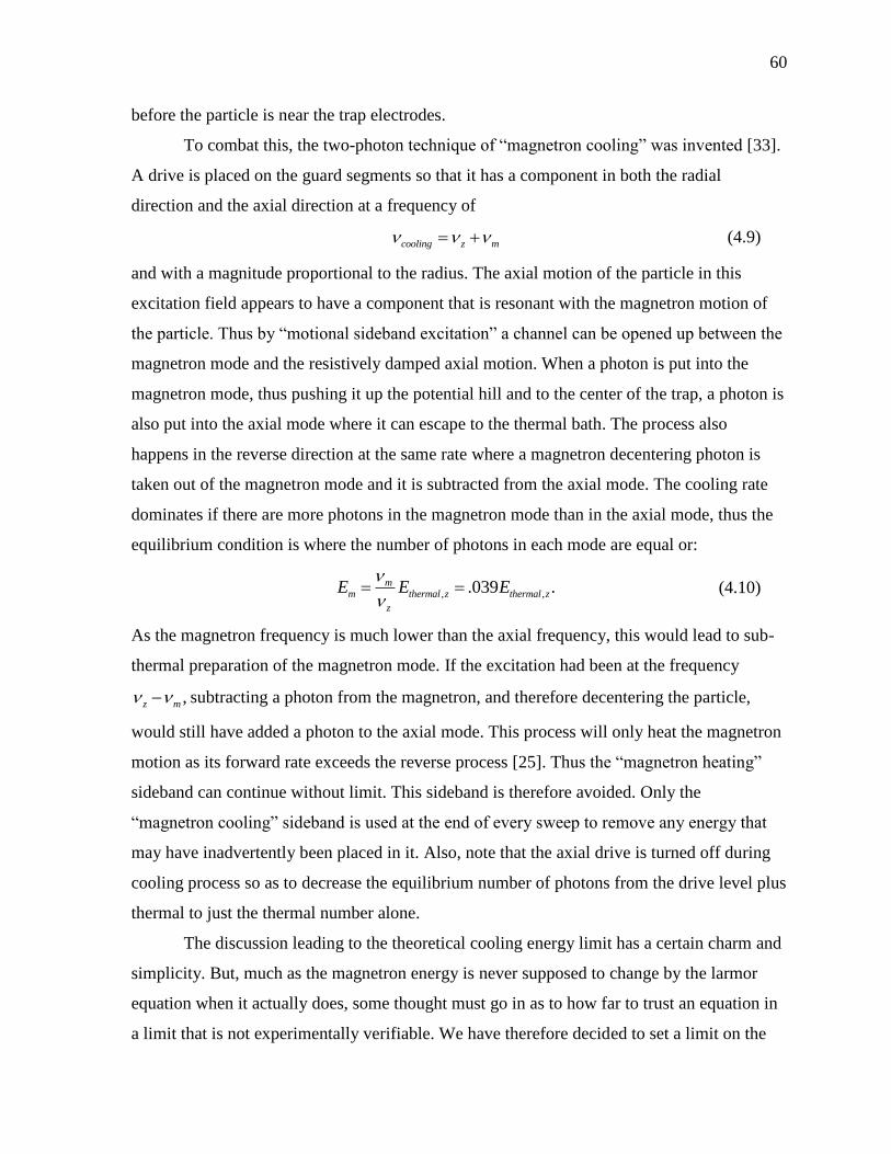
60
before the particle is near the trap electrodes.
To combat this, the two-photon technique of “magnetron cooling” was invented [33].
A drive is placed on the guard segments so that it has a component in both the radial
direction and the axial direction at a frequency of
cooling z m (4.9)
and with a magnitude proportional to the radius. The axial motion of the particle in this
excitation field appears to have a component that is resonant with the magnetron motion of
the particle. Thus by “motional sideband excitation” a channel can be opened up between the
magnetron mode and the resistively damped axial motion. When a photon is put into the
magnetron mode, thus pushing it up the potential hill and to the center of the trap, a photon is
also put into the axial mode where it can escape to the thermal bath. The process also
happens in the reverse direction at the same rate where a magnetron decentering photon is
taken out of the magnetron mode and it is subtracted from the axial mode. The cooling rate
dominates if there are more photons in the magnetron mode than in the axial mode, thus the
equilibrium condition is where the number of photons in each mode are equal or:
, ,.039 .mm thermal z thermal z
z
E E E
(4.10)
As the magnetron frequency is much lower than the axial frequency, this would lead to sub-
thermal preparation of the magnetron mode. If the excitation had been at the frequency
,z m subtracting a photon from the magnetron, and therefore decentering the particle,
would still have added a photon to the axial mode. This process will only heat the magnetron
motion as its forward rate exceeds the reverse process [25]. Thus the “magnetron heating”
sideband can continue without limit. This sideband is therefore avoided. Only the
“magnetron cooling” sideband is used at the end of every sweep to remove any energy that
may have inadvertently been placed in it. Also, note that the axial drive is turned off during
cooling process so as to decrease the equilibrium number of photons from the drive level plus
thermal to just the thermal number alone.
The discussion leading to the theoretical cooling energy limit has a certain charm and
simplicity. But, much as the magnetron energy is never supposed to change by the larmor
equation when it actually does, some thought must go in as to how far to trust an equation in
a limit that is not experimentally verifiable. We have therefore decided to set a limit on the

61
magnetron energy which is traced to the following experiment:
First, we must measure the magnetron frequency. This is done by sweeping around
the cooling frequency z m on the split guards while observing the response in the lock
loop. When frequency goes through z m the observed axial drive drops away because of
the additional motional sideband axial signal and the control loop becomes unstable,
integrating off. The cooling resonance is swept both up and down and the frequency at which
the loop starts to integrate from both directions is recorded. Half way between these two
points is considered to be exactly z m . Then, since the axial frequency is known exactly
due to the lock loop, the magnetron frequency has been determined. This process usually
determines the magnetron frequency to within 3 mHz. For the free space cyclotron
measurement through the quadrature equation 2.13, this leads to an uncertainty of 0.2 ppt, an
insignificant amount.
An example of the response of the axial lock loop correction voltage one sees when

62
one sweeps the cooling resonance is shown in figure 4.6. As the resonance is approached on
either an upsweep or a downsweep, there is no response in the axial lock loop. Once the
resonance is reached, the magnetron motion in the applied excitation field causes the particle
to see an additional axial drive. This axial drive causes the lock loop to wander off in the so
labeled “drift” region. Once the excitation has gone well beyond the resonance point, the
drive seen from the particle’s magnetron motion is off the main axial drive frequency so a
“beating” response is seen. As a magnetron resonance like this is taken with the axial drive
on, it is not as effective at centering the particle as a normal magnetron resonance sweep. The
number of photons left in the magnetron mode would reflect the driven level of the axial
motion. Sharper magnetron resonances can be taken by using slower sweeps, these allow
more precise location of the magnetron frequency which is taken as the average of the
upsweep and downsweep corner frequencies minus the axial drive frequency.
Once the magnetron frequency can be determined, it can be used with the results from
first order perturbation theory under axial lock conditions presented in Dean Farnham’s
thesis [34]. The part which depends on 4C is:
4 4
0 0
6 6.
2 2AxialLock
m c z zm m
m c m
C E C EE E
qV qV
(4.11)
So, by measuring the magnetron frequency shifts at various opposite 4 ' ,C s then
extrapolating to zero drive, one can arrive at the effective thermal magnetron energies. A
quiescent magnetron energy of
, 0.06(2) m meanE meV (4.12)
is used in our analysis.
For ion work where the cyclotron mode is repeatedly excited and larmor radiation
proceeds to center at a prohibitively slow rate, cyclotron centering is also required. This was
first presented when the3 3 H He mass difference was being measured [9] [35]. Before
this, in the proton measurement, the centering was done by resistors separating sections of a
quartered ring electrode. As the desire for better measurements came about more careful state
preparation was needed. Cyclotron centering is accomplished by a method analogous to
magnetron cooling called “cyclotron coupling.” Since the cyclotron energy increases with
increased excitation, we no longer have the negative well as with the magnetron case. The

63
coupling resonance is scanned around
.coupling c z (4.13)
Like the magnetron case, a channel is opened up to damped axial oscillation and a coupling
limit of
,lim , ,12.7 .coup z thermal z thermalc
z
E E E
(4.14)
This is no longer a sub-thermal limit, but is the best that can be hoped for.
An example of the response of the axial lock loop to a sweep of the cyclotron
coupling resonance is show here in figure 4.7. Note the similarity to the magnetron cooling
resonance. Again, the particle does not respond to the excitation until it reaches resonance, at
which point, the extra effective axial drive causes the axial lock loop to drift off. Then, after
going through the resonance, the real drive and the drive from coupling excitation mixed by

64
the cyclotron motion beat with each other. The centering process, like in the magnetron
cooling case, is not as effective when the axial drive is on. However when the process is done
in the dark (as is the case for both the cooling and coupling process during the state
preparation between cyclotron sweeps) we cannot observe the process.
Again, just like for the magnetron case, we are not content to rely on just a theoretical
energy limit for the coupling process. A measurement of the residual cyclotron energy can be
arrived at with the following experiment. Again, by first order perturbation theory, shifts in
the cyclotron frequency can be calculated by again looking at the 4C dependent part of the
shifts calculated in [34]
2 2
4
0
4
0
'
'
3
2
3 1 1 .
2 148 148
AxialLock
c z zzc
c c c m c c m
zc
CE E
qV
CE E
qV
(4.15)
Again, by measuring the cyclotron frequency shifts at opposite values of the electrical
anharmonicity 4 ,C and by taking the measurement at various axial drives and extrapolating to
0 drive, and finally by taking into account the previous magnetron measurement, the
following baseline energies can be arrived at:
,
,'
0.91(55)
30(20) .
mean
mean
z
c
E meV
E meV
(4.16)
Again, this does not really rule out a completely 4.2K system with energies determined by
the Einstein coefficients which would be:
'
14
0.36
4.6
m
z
c
E eV
E meV
E meV
(4.17)
as some groups have assumed, but we feel more comfortable with the experimentally derived
numbers.

65
Section IV.4 Perturbations from Residual Mode Energy and Axial Systematic
Now that we have established how well our centering technique works, it is time to
determine how much the residual mode energies impact the measurement. These
perturbations are calculated in ref [25], but these calculations do not take into account the
fact that a lock loop is operating. As stated before, since this is calculated in Dean Farnham’s
thesis [34], I will divide them up into 3 parts as the expression is rather large. The magnetic
bottle terms are:
6 8
, 22
, 2,
'
'
24 8
0.079.
c quad
c quad zB lock
z mc
z
c
BE E E
m B
where
(4.18)
Next comes the relativistic perturbations:
2 2 4
, 2
2
, ,
'
1 11 .
2 2 8 4
c quad
c quad relativity lock
z mcE E Emc
(4.19)
And lastly come the perturbations from electrical anharmonicity:
4
4 8 2 4 4 8, 4
, 0,
'
3.
2 4 2 2 2 4
c quad
c quad C lock
z mc
CE E E
qV
(4.20)
These are summed for a total:
4
, , , ,
, , , ,, 2, , ,
.c quad c quad c quad c quad
c quad c quad c quad c quadtotal lock B lock relativity lock C lock
(4.21)
For each run these are summed up and a correction is arrived at that varies from -8 to +8 ppt.
Exactly what those corrections are for each run will be dealt with in chapter V.
The perturbations discussed so far in this section result from the thermal energy left
in the modes. In order to lock the particle reliably, it must be driven to a level higher than
this. A level of about 10 times thermal is commonly used in practice. This also creates
perturbations through the anharmonic terms which are given in Farnham [34] as:
2 2 2 42 4
2 2
0 '
31 1 5 1 11 .
2 8 2 4zaxial lock
cz
c
B CE
m B mc qV
(4.22)
These perturbations need not be calculated since they can be determined very accurately by
66
measuring the trap cyclotron frequency of the particle at several different axial drive powers
(in our case, we vary the ring modulation strength which is effectively the same) and
extrapolating back to zero drive. Typical corrections are on the order of -5 mHz for
deuterium and -1 mHz for carbon out of approximately 45 MHz. Note that because the
carbon has more charge and a greater mass, its motion can be detected more reliably with a
much smaller axial excursion – this is why the carbon axial systematic is smaller than the
deuterium axial systematic. Regardless, several days at the beginning and on the end of each
mass comparison are devoted to measuring these shifts.
Section IV.5 Image Charge Effect
In order to do the experiment, we must load an ion into the trap. At first glance, it
would seem that loading a large cloud of ions of the species of interest would be desirable.
Because of the increased charge, the coupling to the tuned circuit would be larger and thus so
would the signal. It should be noted that as the line-width is now a multiple of the single
particle line-width and therefore the phase uncertainty gives a larger systematic.
Compensating for this, partly, would be that with the increased signal to noise, the phase of
the particle relative to the stable synthesizer can be measured more accurately. When
convenient, the phase of the particle is better measured on multiple ions. The real issue with
multiple ions in the trap is the image charge systematic associated with it.
A charged particle placed near a conducting surface interacts with that surface so it
should not be surprising that there is a measurable effect when placing a charged particle in
an instrument as sensitive as a Penning trap mass spectrometer with our resolution. Figure
4.6 shows an approximation where the hyperbolic trap is replaced by a box trap (rectangular
prism). The infinite array of image traps and image charges is represented here. Noting this
approximation’s similarity to the case of an ionic crystal, the interaction can be seen to be
attractive (note the hard core repulsion of the Pauli exclusion principle is replaced by the
electric and magnetic confinement of the Penning trap). This strengthens the radial electric
field which weakens the effective magnetic field seen by the particle and therefore reduces
the trap cyclotron frequency. It provides an extra attraction to the endcaps which weakens
axial confinement and lowers the axial frequency. This in turn is corrected by the lock loop

67
to no net effect except for lock loop’s influence on the magnetron and cyclotron mode
frequencies. It also provides an extra radial E field that increases the E in the E B motion to
increase the EB
velocity and thus the magnetron frequency.
Various degrees of sophistication can be applied to calculating the image charge
effect. Our group uses the spherical image charge approach on an averaged radius to arrive at
the frequency shift [36]. P.B. Schwinberg has done relaxation calculations internally on trap
geometries expressed in coordinate systems where the trap electrodes are simple. Another
68
author uses a Legendre polynomial expansion of the trap and electrode imperfections to
calculate the image charge shift [37]. All find a 31
rdependence of the shift on scaled trap
size. We have chosen to measure the shift by loading various numbers of the same ion into
the trap, counting them, then measuring the cyclotron shift. Using this method, we have
arrived at an image charge shift of [31]
2.23(9) mHze (4.23)
in our trap that must be added to the cyclotron frequency and subtracted from the magnetron
frequency in order to get to the empty trap frequencies. It may be noted that reference [36]
predicts that the sum of the trap frequencies, c mv is invariant regardless of the number of
ions in the trap. The invariance of this sum has been verified experimentally.
Section IV.6 Ion-Ion Interactions, Ion Loading, and Ion Cleaning
We have established the need for limiting the number of particles in the center of the
trap to one. Though the ion loading process is somewhat selective, many other ions are
produced. These form a cloud in the trap around the ion of interest. The effect of space
charge has been widely studied [38] [39]. The cloud quickly forms an ellipsoid of uniform
density which produces an additional radial force on the particle. Wineland gives the formula
for the cyclotron frequency perturbation as:
2 2 162
3
2
c c z
c
q a
m
(4.24)
where ‘a’ is the radial size of the cloud of particles of charge density . This can be
rearranged, Taylor expanded given the rough approximation 2 2 2
c z c , and rewritten:
,
2
8
3
c I
c
c
c
a
B
(4.25)
where B is the magnetic field of 5.9 T and defining the mean cyclotron frequency of the
cloud ion to be ,c I . For a representative load of 1450 N ions in a 2 mm radius ball (i.e. near
0 ), this would yield a fractional frequency deviation of 32 10 . It should also be noted that

69
this is most applicable to the cyclotron frequency of a small cloud of particles. However, if
the ion of interest is at the center of a spherical shell of charge in a region without charge,
there is no radial force to generate the perturbation – some of the charge must reside inside
the magnetron orbit of the particle for there to be an effect. Thus, this mostly explains the
difficulty taking a cyclotron resonance on a dirty cloud of ions early in the ion cleaning
process.
Let us discuss the effect of like ions that are far enough from the trap center so that
they are not found on the tuned circuit. This has no space charge effect because the
interfering ion is not “inside” the magnetron orbit of the ion of interest. As discussed in
chapter 3, the number of particles of like charge to mass ratio in the center of the trap can be
counted because the axial line-width of the particle is proportional to the number of particles
coupling to the tuned circuit. This is measured by turning off the lock loop and scanning the
axial frequency on the drive synthesizer through the standard attenuators. If you watch the
output of the properly phase adjusted lock-in detector you will see a dispersion shape. The
distance between the minimum and maximum of the dispersion curve is the axial line-width
of the particles in the trap and a multiple of the single particle line-width. Fitting this curve to
its ideal shape is also a measure of how far the phase is off from ideal. This allows the phase
of the lock-in detector to be calibrated. In later runs, this was specified to within 2 degrees,
but in earlier runs, less care was taken.
If a second particle is in the trap, but off center, it will have a different axial
frequency because of the rapidly increasing potential from the 6C and higher order Legendre
polynomials that come from the axial hole in the electrodes, the guard electrodes, and any
electrode imperfections. This was seen experimentally when positrons were loaded off axis
during the positron/electron experiments in the 1970’s and 1980’s. Particles loaded 1/3 of the
way out from the center had axial frequencies that differed by over 1 part in 100 from the
central tuned circuit frequency. This required the adjustment of the trap potential to cool their
axial motion and the sweeping of the voltage as the particles were centered by pushing them
up the magnetron energy hill with magnetron cooling. (Note that in a perfect Penning trap,
with no holes and infinite electrodes, there is only 2C , the quadrupole term.) The higher
order terms become more prevalent off trap center and at higher axial drive levels. It should
also be noted that even at low drive levels, terms beyond 4C probably form a small bottom

70
limit for the baseline harmonicity of the trap - limiting the noise shorting. Regardless, if a
particle is loaded far off center, it will most likely not be seen on the tuned circuit, and so it is
undetectable in this way.
In spite of this, the off axis particle does produce an effect on the experiment. This is
a real effect and can be seen when our techniques used to isolate a single particle are not
employed. There are two effects that generate this pulling of frequency, the first is a resonant
coupling between the ion of interest and another ion with the same charge to mass ratio (to be
discussed with equations 4.34 through 4.42). The second is from when a particle of a
different charge to mass ratio (and therefore off the tuned circuit) is relatively close to the ion
of interest. At this point the coulomb force from the particle rotating around at a different
magnetron frequency rf-modulates the cyclotron EM force, causing a slight depression of the
cyclotron frequency by a process similar to the rf-trapping effect of the ring modulation. This
can be seen in the following derivation.
First, let us derive a few basic relations between the fundamental frequencies of the
trap. From equation 2.9, it is easy to see that:
2 2
.2 2
z zc m m
c
(4.26)
Also note that from equation 2.9:
.c c m (4.27)
Now taking the differential form of the second half of equation 4.26 and combining with
4.27, we get:
2 2 2
.m c mz z z
m z c z c z
(4.28)
And from the previous two equations and the invariance of c , the free space cyclotron
frequency, we get
2 2
.c mz zc m m
z c z c
dd d
(4.29)
Now that the preliminaries are finished, let us examine the case where a charged
particle is swinging around the particle of interest at a different magnetron frequency than the
particle of interest. The interaction is coulomb and only dependent on the distance between
the two particles. As long as the spacing between the ions is large compared with radius of

71
the cyclotron mode, lateral distance is unimportant and the equations of motion can be
written:
2
2
cos 0
1 cos 0.
m
c m
c
mx k t x
x t xm
(4.30)
This is the equation of a harmonic oscillator where there is an extra modulation that is fast
compared to the frequency of interrogation (the scan of the resonance), yet slow compared to
c . This is analogous to the case of our ring modulation, a treatment of which can be found
on page 253 of [25]. Following that example, write 4.30 as:
2 2 20 where 1 cosc mx x t t (4.31)
since both and m
c
are small. The frequency deviation is given as:
2 2
2 4.
16 16
c
c cm
(4.32)
The base spring constant deviation is arrived at by expanding the Coulomb force in a
Taylor series:
0 0
2
2 3
0 0
1 2.
4 4
dFF F x F x
dx
d q q q
dx x x
(4.33)
This is valid as long as the cyclotron orbit is much smaller than the particle spacing. For a
perturber located 0.1 mm from the ion of interest, this leads to a perturbation of about
7pptc
c
for a charge 6 species (such as 6
16O ) influencing the 6
12C cyclotron frequency.
This is an effect that takes place regardless of the species perturbing the particle and falls off
rapidly, decreasing as 2
6
n
r where n is the number of charges on the perturbing species.
Next, let us examine a larger effect – that of resonant coupling between two ions of
like species. We will consider the case where the two ions are far enough away from each
other that they are no longer on the same tuned circuit and therefore cannot be counted as
two ions in the axial resonance. The equations of motion of the two particles can be written
72
as two periodically coupled harmonic oscillators frequencies with slightly different resonant
frequencies:
2
2 2 2
2
( ) cos 0
cos 0
( ) cos 0
( )cos 0
m
m
c m
c m
kx x x x t
m m
k kx x x x t
m m
x x x x t
x x x x t
(4.34)
where 2
c
k
m , 2 2 c c
k
m
, 2
m
with the same definitions of coupling
constants as the last example. Assuming oscillatory motion, this system can be written as the
matrix equation:
2 2 2 2
2 2 2 2 2
2 2 2 2
2 2 2 2 2
cos cos0
cos cos
cos cos0.
cos cos
mi t
c m
m c m
c m m
m c m
D t te
t D t
t t
t t
(4.35)
Note, here I have assumed at this point that is constant, though later I will use the time
average of its variation. This is a type of perturbation solution, and as only an approximate
solution is necessary it is sufficient to state the quantity is small. The system only has
non-trivial solutions if the determinant of the matrix is equal to 0, leading to the following
equation.
2 2 2 2 2 2 2 4 2
2 4
2 2 2 4 2
cos cos cos 0
cos cos .2 4
c m c m m
c m m
t t t
t t
(4.36)
The – branch of this equation is the adjusted frequency of the particle of interest and the +
branch is the frequency of the perturbing particle. So taking the branch of the particle that is
on the tuned circuit we get the following
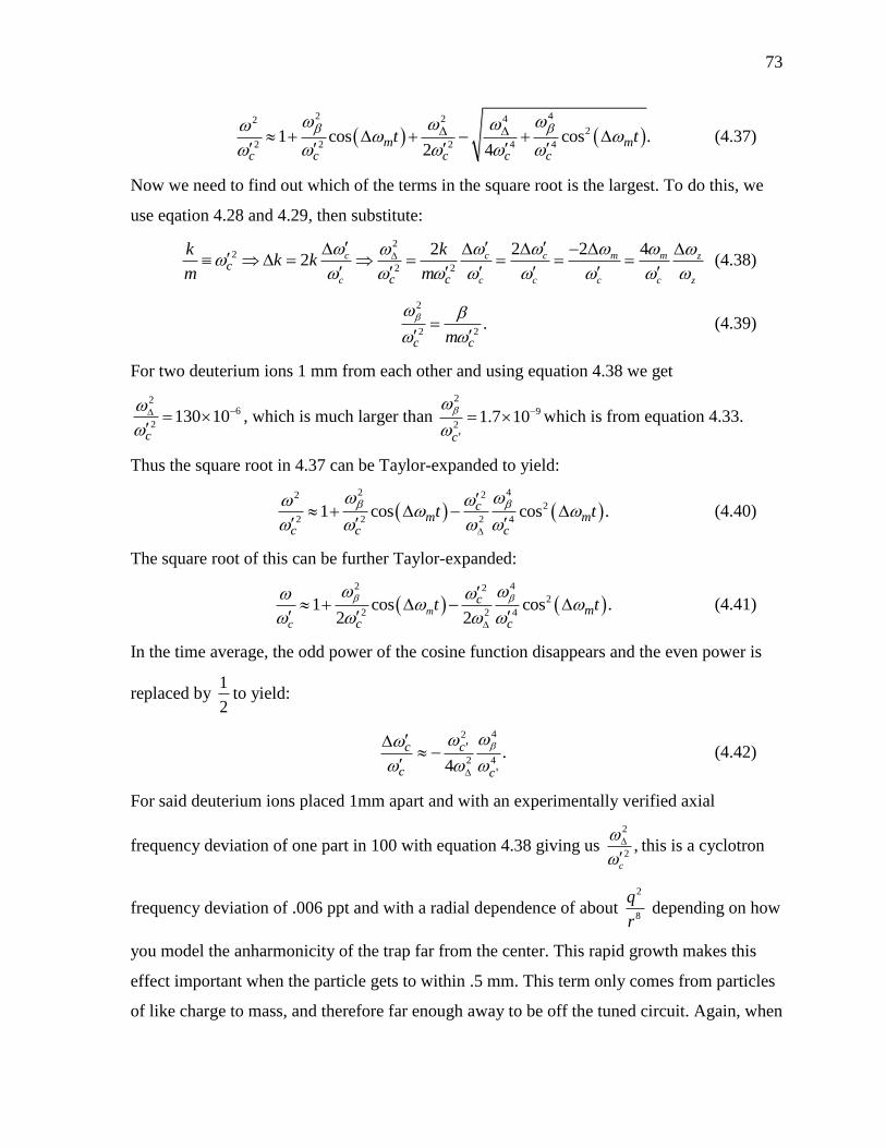
73
2 42 42
2
2 2 2 4 41 cos cos .
2 4m m
c c c c c
t t
(4.37)
Now we need to find out which of the terms in the square root is the largest. To do this, we
use eqation 4.28 and 4.29, then substitute:
2
2
2 2
2 2 422 c c c m m z
c c c c c z
cc c
k kk k
m m
(4.38)
2
2 2.
c cm
(4.39)
For two deuterium ions 1 mm from each other and using equation 4.38 we get
26
2130 10
c
, which is much larger than
2
9
2
'
1.7 10c
which is from equation 4.33.
Thus the square root in 4.37 can be Taylor-expanded to yield:
2 422
2
2 2 2 41 cos cos .c
m mc c c
t t
(4.40)
The square root of this can be further Taylor-expanded:
2 42
2
2 2 41 cos cos .
2 2m
c
cm
c c
t t
(4.41)
In the time average, the odd power of the cosine function disappears and the even power is
replaced by 1
2to yield:
42
2 4
'
'
.4
c c
c c
(4.42)
For said deuterium ions placed 1mm apart and with an experimentally verified axial
frequency deviation of one part in 100 with equation 4.38 giving us 2
2,
c
this is a cyclotron
frequency deviation of .006 ppt and with a radial dependence of about 2
8
q
r depending on how
you model the anharmonicity of the trap far from the center. This rapid growth makes this
effect important when the particle gets to within .5 mm. This term only comes from particles
of like charge to mass, and therefore far enough away to be off the tuned circuit. Again, when
74
they are on the tuned circuit, they will be centered and detected. There is some worry,
however, that over time, the magnetron cooling may act weakly on these particles (remember
magnetron cooling requires the action of a tuned circuit to be effective and therefore the off
resonant particles are only very weakly cooled) and pull them toward the center where they
can affect the measurement. When the particle eventually becomes centered and the coulomb
coupling between the particles is strong, the experiment is only sensitive to the center of
mass of the particles so the image charge effect is the best way to characterize the
perturbation.
The effect of the first two of these three perturbations is exacerbated by the fact that
once the trap was used to measure the3 3 H He mass difference. During this experiment a
small cloud of3 H, a radio-active isotope, was released into the trap. It proceeded to adsorb
on the inner trap surfaces where it continued to beta-decay, sending high energy electrons
across the trap. These hit the trap surfaces and cause the spontaneous loading of random ions
from adsorbed gasses. The trap surfaces were gently scrubbed – reducing the trap activity by
a factor of 410 (this was measured by noting the reduction of the self-loading rate of

75
electrons in the trap when the ring was biased with a positive voltage), but some activity
remained nonetheless.
This, alone, justifies the need for ion cleaning techniques. However there is an even
more important reason they are needed. The loading process produces a vast array of
impurity ions in the trap, and there is no experiment without loading an ion. Refer to Fig. 4.9
for pertinent aspects of the following loading process.
To load deuterium, first, a source was produced by heating a titanium wafer in a
deuterium atmosphere, allowing it to diffuse into the metal matrix. This was then placed in
the vacuum envelope with wires connected to it so that it could be warmed electrically.
During the warming process deuterium diffuses out of the wafer and forms a short-lived
neutral cloud in the Penning trap. The cloud is soon cryo-pumped away by the cold 4.2 K
surfaces of the trap, but as a similar process was used to produce tritium in the past, it is easy
to see how the trap became contaminated with tritium. While the cloud is evolving, a field
emission point (FEP) is biased so that electrons form a beam by tunneling from the region of
high field gradient at its point. This beam is confined to a thin rod shaped volume by the
ambient magnetic field and is reflected by the “reflector” electrode on the other side of the
trap. This folded electron beam reaches a brightness that is almost 610 times that of the
unfolded beam and allows ion production at typical electron currents of 10-20 nanoamps.
Because electrons build up over time between the FEP and the skimmer which choke out the
electron production process, the skimmer is modulated by a high voltage 60 Hz potential
which dumps the electron beam at each cycle. For deuterium production, the electron beam
energy is kept below 100 volts as it crosses the trap so that high charge states of other ions
aren’t produced. These high charge states seek the center of the trap and are difficult to expel.
In the example figure, the beam energy at trap center is 68 volts and the beam energy at the
endcap electrodes is 80 volts.
During the loading process, the trap potential is kept so that protons, the most
prolifically produced ion in this process, are on the tuned circuit, and any proton produced
gets its axial energy damped out to form a small, cold cloud in the center of the trap. The
deuterons produced collide with the ions in this cloud and are cooled in a process analogous
to buffer gas cooling. At the same time, other ions are produced. These are also cooled by the
cloud of protons; however, because of the low electron beam voltage in the trap, the range of

76
ions produced is not large. Soon after deuterium is produced, the wafer heater is turned off
and the trap is allowed to cool back to the ambient 4.2 K. Though metal thermal
conductivities are high at low temperature, insulating trap parts are not, and it is usually a day
after the load before we consider the trap properly cooled for precision work.
6
12C and 4
12C are produced in a similar way, except the process does not inject heat
into the system and a cloud of cold protons is not used to center the ions. Instead, an electron
beam is produced without heating the wafer with an energy around 550 volts at the endcap
electrodes. This beam scrubs neutral carbon off the skimmer electrode, which is left over
from the chemical cleaning process, and ionizes it. This ionized carbon wanders across the
center of the trap where the beam energy is high (note that with a new FEP, the beam energy
at the skimmer is limited to around 200-300 volts so that excessive electron currents are not
produced. With time, the FEP tip blunts from use and the voltage needed to produce the
required current increases to what is shown in the figure). In the center of the trap, the carbon
is successively ionized until it reaches the desired state. This time, the trap voltage is kept so
that the carbon ion of the chosen charge state will be damped on the tuned circuit. When an
ion of the right charge state is produced, frequently a noise spike can be seen on the tuned
circuit as its motion rings down. It takes on the order of a minute for the electron beam to
fully strip a small cloud of carbon. Though several hundred or more ions are easily produced
this way, the best load is where the currents and time are limited so that only a few ions of
interest are produced. This is because the shorter loads also produce fewer unwanted ions to
be culled from the trap.
Now that the ions are produced, the process of cleaning out unwanted ions proceeds.
Initially in the process this is done in two main ways. The first is by applying a swept
“broom” excitation to the drive endcap around the axial frequency of the particle to be kicked
out of the trap. These ions are not on the tuned circuit, so when they are excited, their
oscillations increase in amplitude until they hit the trap electrodes. The “broom” is swept
because the axial frequency changes as the energy increases and we do not want the particles
to fall off resonance. The second technique is used with species which are near the tuned
circuit. With these, direct drive would be dangerous so we excite them with 2 z . This causes
their axial motion to become unstable and, again, hit the trap electrodes. If too many ions of
interests are produced, there will be too much “buffer gas” cooling and we will not be able to

77
properly clean out the trap. Therefore, clouds of much larger than several 100 ions of interest
are not desirable. After the trap is cleaned up somewhat, a magnetron cooling drive can be
applied to center the cloud. At this point, it can be counted either roughly, by looking at the
noise shorting feature width on the tuned circuit, or more precisely, by taking a driven axial
resonance and seeing how wide it is.
To some extent, this process runs through a list of all the ions that could be produced
by the beam, but there are ways of telling which ions are in the trap – at least initially before
their axial energy cools. This is done by sweeping the trap voltage and looking at the rms
noise on the tuned circuit. When we pass the trap over the axial frequency of an “ion of dis-
interest” we will see a spike in the detector noise. The voltage sweeper is heavily RC filtered
so that the noise can be seen – the quieter the voltage source, the sharper and smaller the
clouds of ions that can be seen. The ions show up as peaks on the sweep, but if you perch the
voltage on a particular ion, as expected, you will see that cloud of ions cool and the peak go
away. We can find the peak again by running the broom excitation briefly over the ions to
warm up their axial motion.
I have dealt so far with axial ion throw-out, but not how we reduce a large cloud to a
more manageable size. This is done by “well drops”, of which there are two types. One fast,
and the other slow. They each have different effects and also aid in unwanted ion throw-out.
The first to be developed was the “slow drop.” In this process, the ring well depth is dropped
adiabatically to about -6 volts. Now, nothing is on the tuned circuit so no drives should be
applied. The endcap voltage is slowly brought down from ground to near -6 volts
adiabatically and the most energetic particles are allowed to leave the trap by impact into the
endcaps. Because the magnetron motion is now less defined, particle’s tend to wander out of
the center of the trap. This is another way in which particles could be expelled from the trap,
this time into the ring electrode. Then the endcap voltage is brought back to ground and the
well depth is deepened back to the near -46 or -70 volts needed to have the ions of interest
back on the tuned circuit. Magnetron cooling follows the drop to re-center the particles in the
trap. This technique works especially well if an axial drive broom is applied prior to the
process to excite the unwanted ions – these axially excited ions leave the trap, again, via
collisions with the endcap. Originally slow drops were done by hand by disconnecting lines
and hooking them up to different supplies and making sure that these supplies were not

78
changed during the process so that transient voltage spikes did not accidently clear the trap.
Figure 4.8 shows a circuit I developed to automate the process.
The CA3080A OTA (Operational Transconductance Amplifier) acting into the output
capacitor serves as a combination of follower and ramp generator, bringing down the -6 volt
well in about 2 seconds. It could be argued that the lack of an output buffer is either a
deficiency, or an elegant solution to the risk of sending in high frequency spikes from the
buffer rails. This was the first circuit I designed for the experiment so some latitude is
begged. It could be replaced by an amplified and heavily filtered Arbitrary Waveform
Generator at the cost of reliability, money, and time. As we are familiar with rapid
electronics prototyping techniques, we chose not to go this route.
The fast well drop is used to clear particles from the trap that are not within 140 m
of the center. To understand how it works, one must also understand the endcap termination
networks. These are shown along with the “fast drop” circuit in figure 4.9. The endcap
terminations allow several things to happen. First, for diagnostic purposes, it is necessary to
offset the particle in the trap by putting a positive voltage on one endcap and an negative
voltage on the other. This allows us to take cyclotron measurements, and therefore measure

79
the magnetic field, in different parts of the trap. We can tune out any linear magnetic field
gradient that exists along the axis of the trap. This is desirable because, at some level, the two
ions must be positioned differently in the trap and we wish this to not affect the mass
measurement. Our success in this regard is verified by what we frequently call “control runs”
where the same ion is loaded successively. In all control runs, the mass of the second ion has
proved to be the same as the first to within experimental accuracy. In the termination network
80
for each endcap, there is a 100k resistor to ground at DC. This allows the endcap to be biased
so that the particle can be offset from the center of the trap.
Note the asymmetry of the endcap networks shown in the figure. The signal cap
network is heavily RC filtered at the axial frequency of 3.55 MHz. This prevents any noise
on this line from showing up on the very sensitive cryogenic tuned circuit and preamplifier.
Also, note that external signals are injected at the base of the tuned circuit which is
effectively an AC ground. The same cannot be done for the drive endcap because it must be
able to pass the 3.45 MHz drive sideband to the trap and particle. A frequency selective
network that passes 3.45 MHz, but not 3.55 MHz would be an impractical complication to
the experiment since its Q would have to be well over 100. This could be done but since the
drive endcap is ~4 mm from the signal endcap, the capacitive coupling is minor (~0.1 pf).
Also note that there is about 25 dB of attenuation in this network at signal frequencies. This
attenuation is cryogenic and insures that the particle is only seeing low noise electronics
where it is sensitive.
The asymmetry of the drive and the signal networks is what allows the “fast drop” to
work. First, the ring voltage well depth is again reduced to the same -6 volts used in the
“slow drop” procedure. Next the drive endcap skimmer electrode (figure 1.1) is biased to
+10.5 volts. At this point, the potentials on signal and the drive endcap lines are brought
down quickly to -7.2 volts. Because of the RC time constants on the signal endcap network,
the signal cap drops less than 0.5 volts before the potential is brought back up. The drive
endcap, comes fully down to -7.2 volts because its time constants are far shorter. Thus there
is a strong linear electric field placed across the trap which slams the particles into the drive
endcaps. The exception is the particle at the center of the trap. This particle goes into the 0.3
mm diameter skimmer hole and is reflected back by the positive potential on the skimmer –
essentially trapped in a much smaller asymmetric Penning trap. Theoretically, this would be
a stable configuration for at least several RC time constants of the signal cap network (a few
milliseconds,) however we have found experimentally, that the reliable storage time is less
than 25 microseconds. This is probably because the skimmer gets charged during ion loading
and causes strong lateral fields in the skimmer hole. These cause E B drift in the hole which
cause the particle to impact the electrode, an effect also seen in earlier e+/e- double-trap
transfers. A fast drop with 10 microseconds spent at -7.2 volts and 10 microsecond edge

81
speeds is slow enough that the drive endcap is well equilibrated and yet the particle does not
have time to wander out. The particle of interest has never been lost on a fast drop when it
was well centered before the process. Fast drops were usually performed as daily
maintenance to keep off-axis particles from staying in the trap. They could also be used to
pare down a large cloud shortly after an ion load. They were done after a slow drop because
the slow drop has the tendency to decenter unwanted particles in the trap as well as the
desired particle. A fast drop would therefore expel any particle that was further out than
about 0.15 mm from the center of the trap. Such a particle would already be on the tuned
circuit and therefore be countable. The axial frequency deviation of such a particle can be
estimated by the following formula:
2
0.01 1 .0.90
z z
rkHz
mm
(4.43)
This conservative estimate is within the 1.4 kHz tuned circuit half-width.
The fast drop circuit, like the slow drop circuit, uses an OTA to generate a ramp to
prevent a fast edge from ringing the tuned circuit. The edge speed is dialed in by the Digi-
Pot. The 6 nF capacitor on the OTA output was chosen so that the edge speed would be
approximately 3.75 plus half the reading on the digipot in microseconds. The two FETs
configured as an inverter produce a simple level changer, allowing the voltage of the well
drop to be adjusted. A level-changer or pin driver chip could have been used instead. The
bias current in the output driver can be adjusted by changing the values of the 66 ohm
resistors. We were running at 8 milliamps, but this is probably excessive. A value of 50 ohms
would be sufficient here. We had no adverse effects on the life of the box, regardless of the
output section overdrive. Originally, we figured a much slower drop would be sufficient, but
this ejected the particles from the trap by the aforementioned mechanism.
There is one more type of frequency broom that was used in the deuteron experiment
– that was a cyclotron broom. Species like 2H , the hydrogen molecule with a charge
stripped off, were extremely hard to eliminate with standard methods because its normal
mode frequencies were so close to the species of interest. A swept broom excitation was used
on the intruding ion’s cyclotron mode to blow up its cyclotron orbit to where it could be
eliminated by the fast well drop technique. This technique tended to improve the scatter in
the cyclotron frequency data.

82
To summarize, the loading process involved firing up the FEP, followed by the
application of strong axial ion throw-out brooms to get rid of low charged states of unwanted
ions. Next the trap contents were scanned by looking in the axial noise over scanned ring
voltages and selective ion throw-outs were used on the remaining unwanted species. The
large cloud was then pared down by slow drops, followed by magnetron cooling, then a fast
drop to get rid of particles that had been decentered during the slow drop. At this point, the
process can be repeated until the cloud size as measured in the axial resonance was reduced
to one ion in a slow drop. At any point during this process, 2 z axial throw-outs can be used
on ions particularly close to the tuned circuit. This process generally takes 4-8 hours to
complete. In addition, during the data taking process, frequently the brooms, both axial and
cyclotron were applied during the state preparation intervals after a sweep.
If at any point two particles of interest were left in the trap, this produced a special
problem. The tuned circuit could damp out the center of mass motion, but leave the mode
with the ions swinging with odd symmetry around the trap center (the so called breathing
mode). Then, on a slow drop, the particles of interest would frequently both leave the trap as
there was still an excited axial mode. This chance could be reduced by putting 0
4
V volts on
the trap for a time to bring the excited mode onto the tuned circuit where it could be cooled.
The efficacy of this technique could be verified by exciting the particle of interest directly at
2 z and seeing the response in the axial lock loop through the 4C term. Then, after putting
0V on the trap, the axial lock loop correction signal would return to its previous level. This
procedure was not necessary for numbers of ions greater than two, presumably because ion-
ion scattering proved sufficient to pump the main axial mode where energy could be taken
out of the particle with the tuned circuit operating on the center of mass.
83
Chapter V: Data, Analysis, and Results
This chapter includes the results of the measurement of the deuterium to carbon
cyclotron frequency ratios, it discusses how the systematics are incorporated, and it provides
the final deuteron, deuterium and neutron masses.
Section V.1: Data Analysis and How the Systematics Were Applied
We have already discussed the major systematics in chapters III and IV: axial power,
image charge, range effect, axial phase shift, and residual mode energy. These systematics
modify the three normal mode frequencies as follows:
, ,
,
, ,
, ,
,
0.0291 9 0.00223 9
1tan
2
quad measured axialpower range image
measured axialpower sweep charge
quad synthesizer linewidth
mag quad mag measured image
cooling synt
c c
c
z z
z
N Hz
0.00223 9 .hesizer chargeN Hz
(5.1)
These frequencies are used in the quadrature equation (equation 2.13) to get the free space
cyclotron frequency at each point in time. The time chosen for this data point is the average
of the up-sweep and down-sweep corner times and the frequency for the data point is the
average of the up and down sweep corner frequencies. The magnetron frequency is measured
at either or both of the beginning or end of the run for each ion. The phase for the electronics
is usually measured at the beginning of each deuterium run, and at the end of each carbon
run.
The axial power systematic is measured for each ion, for every run. For deuterium,
this is done at the beginning of the run, and for carbon, at the end of the run. To accomplish
this, cyclotron frequency data points are taken at different axial drive powers. Usually, the
axial power is changed once per day. It is common to use the lowest axial drive that produces
good signal to noise as this reduces the uncertainty in this systematic and tends to produce
the data with the lowest scatter. To measure the axial systematic the raw trap cyclotron

84
frequency data is fit to the following function:
2
, , ,
i
c meas c true ax dr ax i
m
V c t (5.2)
where m is taken out to some convenient power of the time to get rid of baseline frequency
wander. With ax thus determined, the residual axial systematic is calculated by multiplying
with the drive voltage used in the run squared. This number is subtracted from the cyclotron
data to get the true cyclotron frequency. Sometimes, several axial powers were used in a run;

85
in those cases, the proper axial systematic was subtracted from the corresponding data points.
The parameters were obtained from the data using a standard Ordinary Least Squares (OLS)
fit that can either be derived, or looked up in any standard statistics reference [40]. A sample
of the data from a deuterium axial systematic determination is shown here in figure 5.1. The
axial drive in mV is labeled by the data it corresponds to. The scatter for carbon axial
systematic data is smaller than that of deuterium data so the carbon axial systematic is
determined with more accuracy. Note that less effort is required to clean up the particle and
make the data free of systematics since it is less critical at this juncture.
After the axial systematic on deuterium is taken, the main run begins. After some
number of hours taking cyclotron data on deuterium, a carbon atom is loaded and cyclotron
data is taken on that species. The trap cyclotron data is changed to the free space cyclotron
frequency, then fit to the following functions:
2
1 1 2 3 3 4 4
1 1 2 3 3
1 1
1 1
1 for 0.
1 for 0
Q
L
model c c t c t c t or
model c c t c t
tt
t
(5.3)
The i scale parameters are constants to make the components of the hessian of the objective
function roughly the same order of magnitude for numerical efficiency. Extra fit parameters
in the second bracket such as lab temperature and pressure were added in on a trial basis;
however no consistent coefficients were observed so these fits were dropped.
The error bars on the individual observations were determined in two different ways.
The first is with a variant of “Feasible Weighted Least Squares” (FWLS) where I found the
error bar that makes the reduced chi-squared statistic, 2 , equal to one for the data of a
given ion. This was an iterative procedure that converged well within 2-3 trials. This gives a
smaller error bar for the carbon data than the deuterium data. The second method is to use the
error from the corner determinations from the supervisor program of the sweep interpreter.
This weights the points in a way that varies from point to point. In general this error is also
less for carbon than for deuterium and is smaller when the sweep interpreter fits the up-
sweep and down-sweep models better. This second method gives error bars that are
significantly smaller than the scatter, but weighted towards the better points. Any bias from

86
this method of weighting points was measured in the determination of the “range effect.” The
error bars must be scaled in the end to make the reduced chi squared statistic, 2 , to be one.
I did fits with model functions that included both linear and quadratic magnetic field time
dependence (see equations 5.3) then took a weighted average of the results to get the final
run result. This result was corrected by the amount necessary to account for the mean
residual energy left in the three modes through equations 4.18, 4.19, and 4.20. The
corrections in ppt are shown in table 5.1.
The MATLAB code for fitting the model function is included in Appendix B. Since
the model functions are non-linear, it uses an iterative approach. Instead of a more
conservative method such as the Levenberg-Marquardt method, the quality of our data allows
for the more aggressive approach of a generalization of Newton’s Method which can be
found in a reference such as [41]. The iterative procedure is given by:
1
2
2
1.
N N N
k j N N j N
data
N i i
i i
x x p
S x p S x
S x model data
(5.4)
This would converge to within machine precision in well under a second of machine time
with standard initial conditions even with the plotting of the residuals at each step.
The final cyclotron frequency ratio is arrived at by the following formula:
2
2
1
1
cCFR
c
(5.5)
from the fit results. The errors on the fit parameters are taken from the diagonal terms of the
traditional estimated covariance matrix as follows:
2
1
,m j k m mc S x
(5.6)
where 2
is the scaling factor necessary to make the reduced chi squared statistic, 2 , equal
to one. For the first method of determining the error bars, this was approximately equal to
one, for the second method, it was on the order of 15-20. Note that the traditional covariance
matrix is inverted from a hessian with one term while the hessian of the objective function S,
strictly speaking, has two terms, one of which is zero when the parameters are properly fit.
Both estimates of the covariance matrix were calculated and the results were the same for the
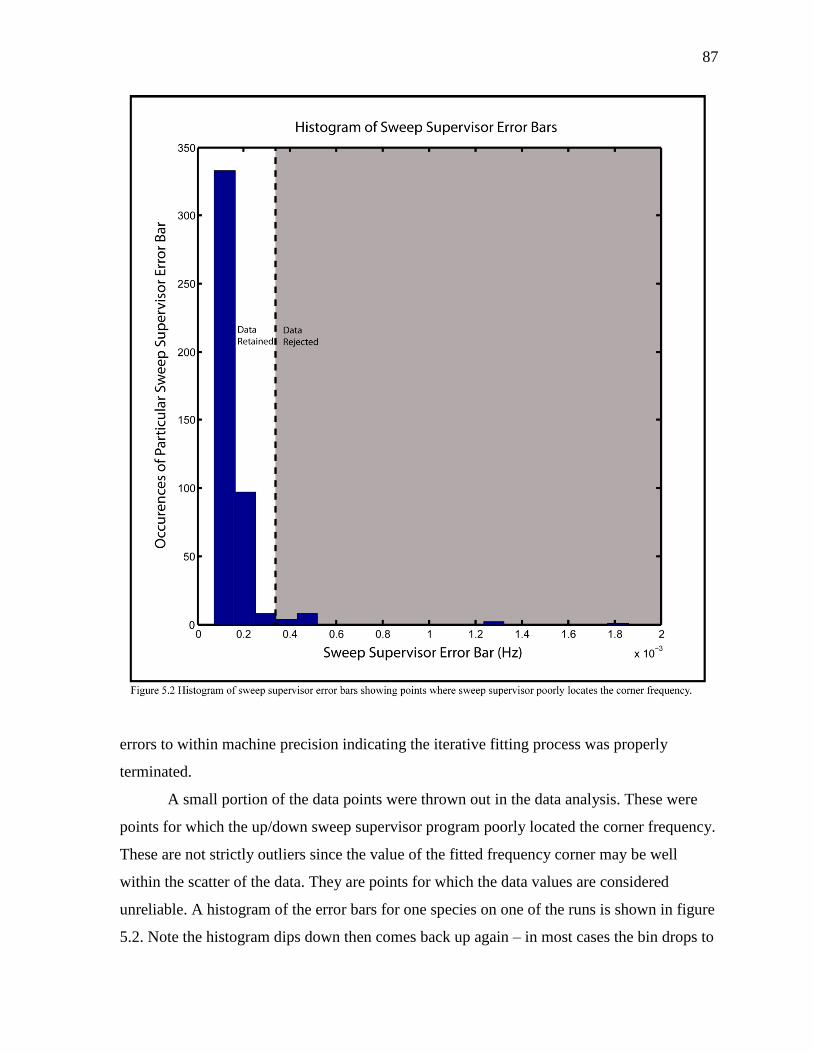
87
errors to within machine precision indicating the iterative fitting process was properly
terminated.
A small portion of the data points were thrown out in the data analysis. These were
points for which the up/down sweep supervisor program poorly located the corner frequency.
These are not strictly outliers since the value of the fitted frequency corner may be well
within the scatter of the data. They are points for which the data values are considered
unreliable. A histogram of the error bars for one species on one of the runs is shown in figure
5.2. Note the histogram dips down then comes back up again – in most cases the bin drops to
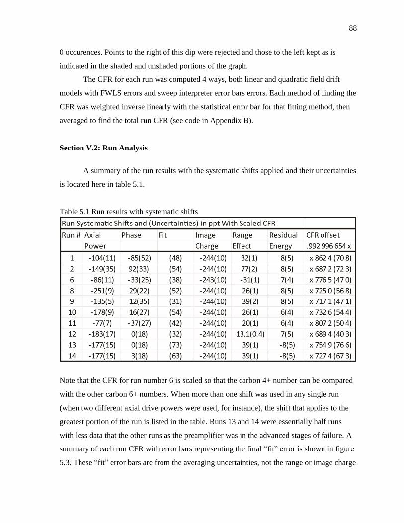
88
0 occurences. Points to the right of this dip were rejected and those to the left kept as is
indicated in the shaded and unshaded portions of the graph.
The CFR for each run was computed 4 ways, both linear and quadratic field drift
models with FWLS errors and sweep interpreter error bars errors. Each method of finding the
CFR was weighted inverse linearly with the statistical error bar for that fitting method, then
averaged to find the total run CFR (see code in Appendix B).
Section V.2: Run Analysis
A summary of the run results with the systematic shifts applied and their uncertainties
is located here in table 5.1.
Table 5.1 Run results with systematic shifts
Note that the CFR for run number 6 is scaled so that the carbon 4+ number can be compared
with the other carbon 6+ numbers. When more than one shift was used in any single run
(when two different axial drive powers were used, for instance), the shift that applies to the
greatest portion of the run is listed in the table. Runs 13 and 14 were essentially half runs
with less data that the other runs as the preamplifier was in the advanced stages of failure. A
summary of each run CFR with error bars representing the final “fit” error is shown in figure
5.3. These “fit” error bars are from the averaging uncertainties, not the range or image charge

89
effects.
The run trap-cyclotron-frequency residuals of the quadratic field drift, fitted with
bootstrapped errors, is presented here in figures 5.4 through figure 5.13 with a normal plot of
the scaled residuals for each run. A normal plot is a way of looking at the normality of the
residuals of the data and fit. First, the residuals are sorted. The X-axis is the residual and the
Y-axis is the probability of the data ordered by the residual and scaled in such a way that a
Gaussian normal distribution creates a straight line. The line in the plot is determined from
the first and third quartile of the data. To plot both ion’s data on the normal plot, the residuals
are scaled by the ratio of the bootstrapped error bars.
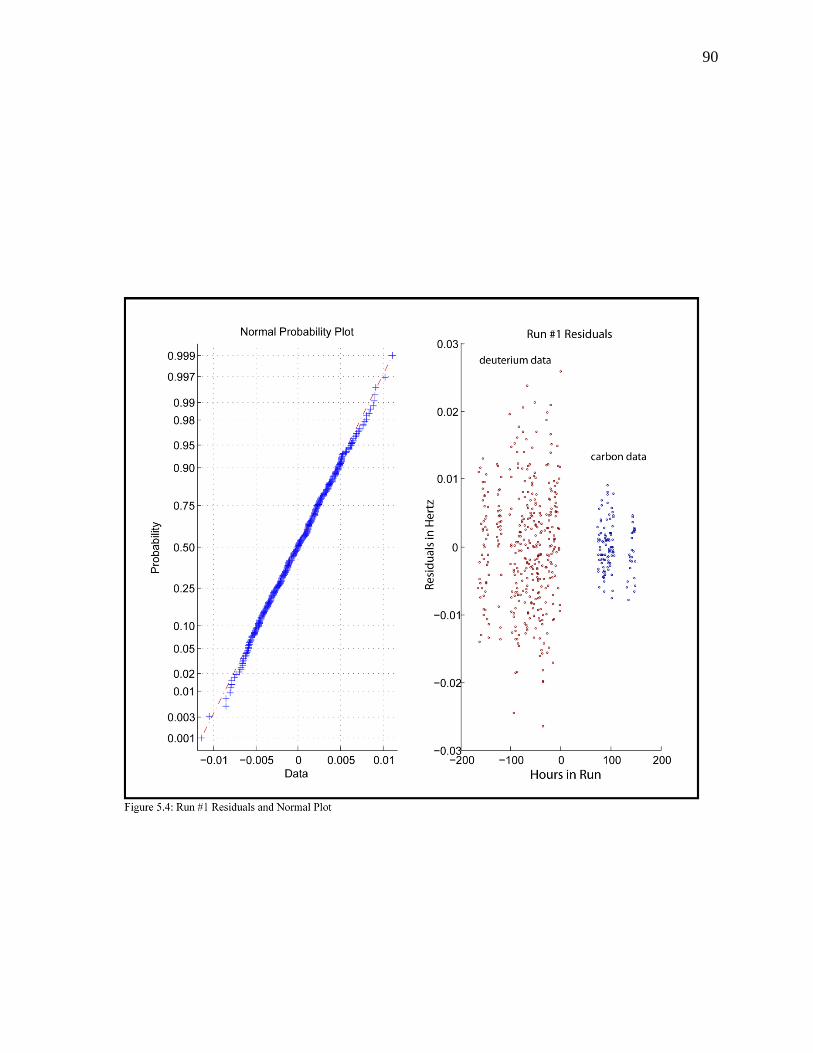
90

91

92
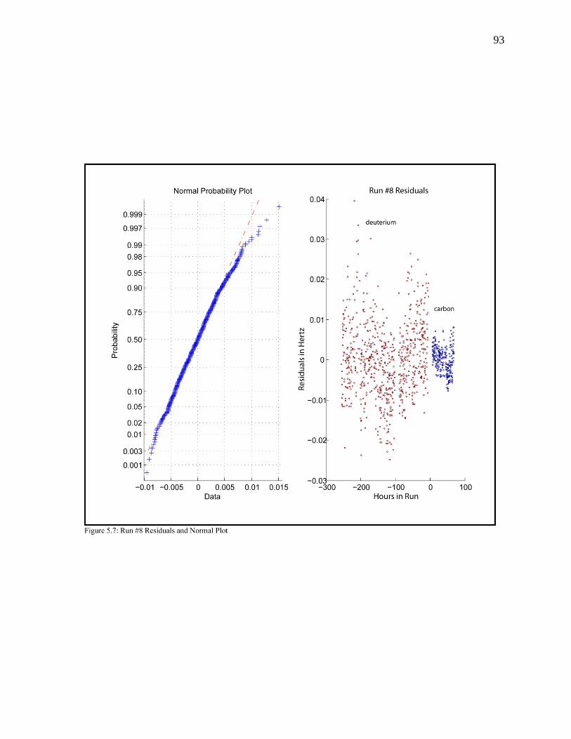
93
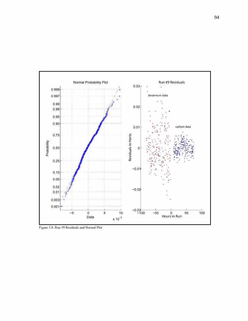
94

95
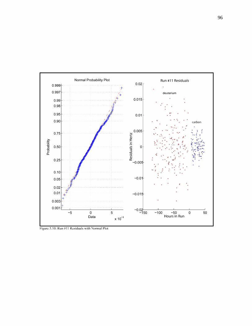
96

97

98
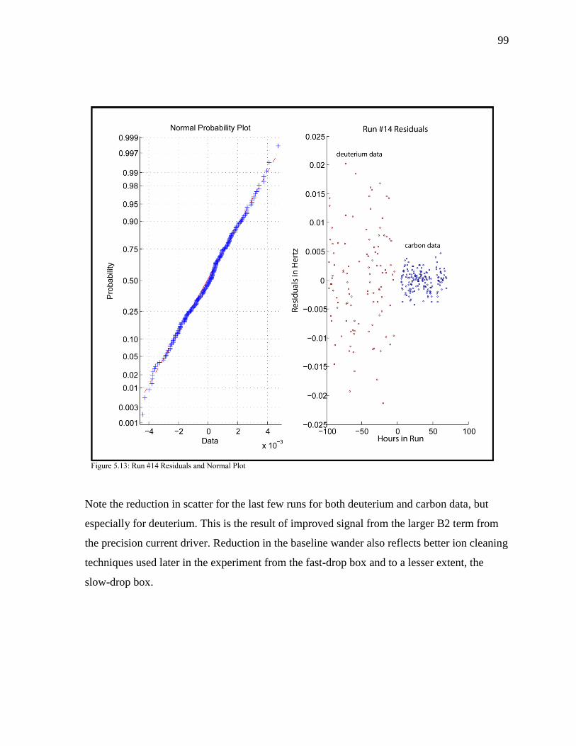
99
Note the reduction in scatter for the last few runs for both deuterium and carbon data, but
especially for deuterium. This is the result of improved signal from the larger B2 term from
the precision current driver. Reduction in the baseline wander also reflects better ion cleaning
techniques used later in the experiment from the fast-drop box and to a lesser extent, the
slow-drop box.
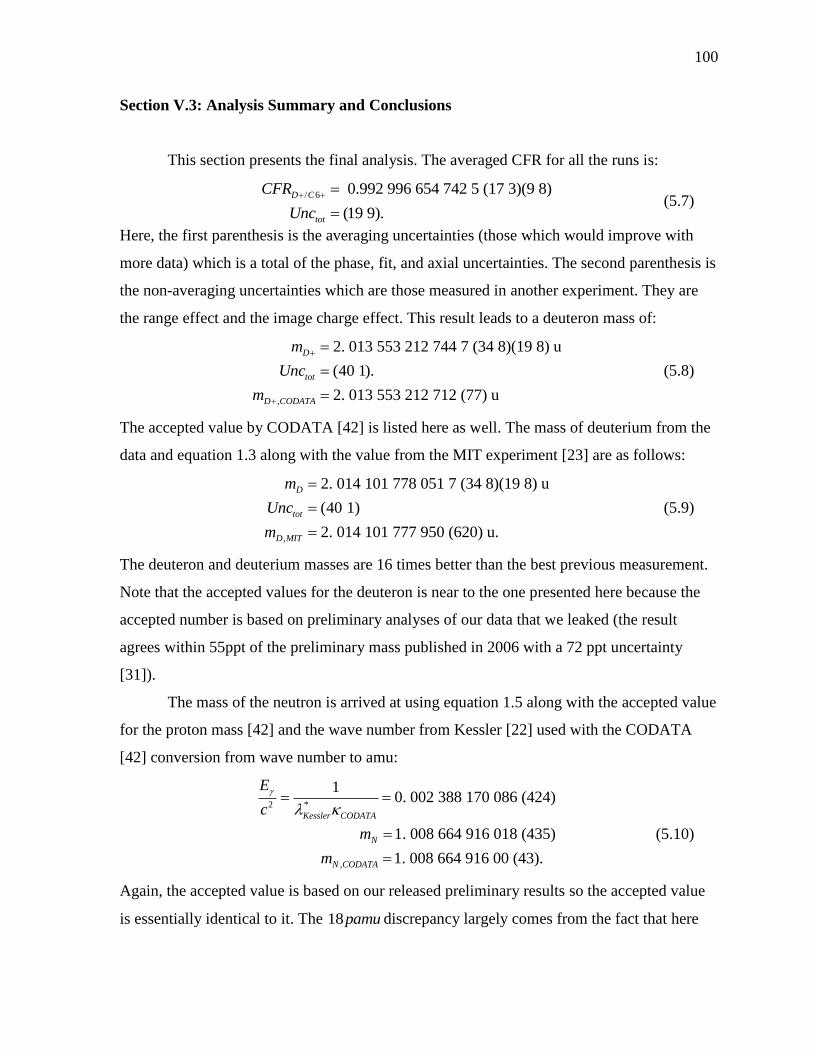
100
Section V.3: Analysis Summary and Conclusions
This section presents the final analysis. The averaged CFR for all the runs is:
/ 6 0.992 996 654 742 5 (17 3)(9 8)
(19 9).
D C
tot
CFR
Unc
(5.7)
Here, the first parenthesis is the averaging uncertainties (those which would improve with
more data) which is a total of the phase, fit, and axial uncertainties. The second parenthesis is
the non-averaging uncertainties which are those measured in another experiment. They are
the range effect and the image charge effect. This result leads to a deuteron mass of:
,
2. 013 553 212 744 7 (34 8)(19 8) u
(40 1).
2. 013 553 212 712 (77) u
D
tot
D CODATA
m
Unc
m
(5.8)
The accepted value by CODATA [42] is listed here as well. The mass of deuterium from the
data and equation 1.3 along with the value from the MIT experiment [23] are as follows:
,
2. 014 101 778 051 7 (34 8)(19 8) u
(40 1)
2. 014 101 777 950 (620) u.
D
tot
D MIT
m
Unc
m
(5.9)
The deuteron and deuterium masses are 16 times better than the best previous measurement.
Note that the accepted values for the deuteron is near to the one presented here because the
accepted number is based on preliminary analyses of our data that we leaked (the result
agrees within 55ppt of the preliminary mass published in 2006 with a 72 ppt uncertainty
[31]).
The mass of the neutron is arrived at using equation 1.5 along with the accepted value
for the proton mass [42] and the wave number from Kessler [22] used with the CODATA
[42] conversion from wave number to amu:
2 *
,
10. 002 388 170 086 (424)
1. 008 664 916 018 (435)
1. 008 664 916 00 (43).
Kessler CODATA
N
N CODATA
E
c
m
m
(5.10)
Again, the accepted value is based on our released preliminary results so the accepted value
is essentially identical to it. The 18pamu discrepancy largely comes from the fact that here

101
we have used the more recent conversion from wave number to amu, whereas the accepted
value seems to use the outdated one from the 1999 Kessler paper. If we were to look at a
neutron mass computed from the next best deuteron measurement [23], the uncertainty would
be 74 u . Our number is only a 40% improvement over this since the bulk of the uncertainty
is now the gamma ray binding energy measurement, not the proton or deuteron masses.
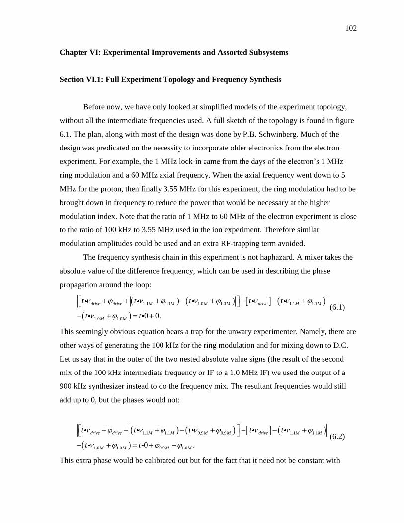
102
Chapter VI: Experimental Improvements and Assorted Subsystems
Section VI.1: Full Experiment Topology and Frequency Synthesis
Before now, we have only looked at simplified models of the experiment topology,
without all the intermediate frequencies used. A full sketch of the topology is found in figure
6.1. The plan, along with most of the design was done by P.B. Schwinberg. Much of the
design was predicated on the necessity to incorporate older electronics from the electron
experiment. For example, the 1 MHz lock-in came from the days of the electron’s 1 MHz
ring modulation and a 60 MHz axial frequency. When the axial frequency went down to 5
MHz for the proton, then finally 3.55 MHz for this experiment, the ring modulation had to be
brought down in frequency to reduce the power that would be necessary at the higher
modulation index. Note that the ratio of 1 MHz to 60 MHz of the electron experiment is close
to the ratio of 100 kHz to 3.55 MHz used in the ion experiment. Therefore similar
modulation amplitudes could be used and an extra RF-trapping term avoided.
The frequency synthesis chain in this experiment is not haphazard. A mixer takes the
absolute value of the difference frequency, which can be used in describing the phase
propagation around the loop:
1.1 1.1 1.0 1.0 1.1 1.1
1.0 1.0 0 0.
drive drive M M M M drive M M
M M
t t t t t
t t
(6.1)
This seemingly obvious equation bears a trap for the unwary experimenter. Namely, there are
other ways of generating the 100 kHz for the ring modulation and for mixing down to D.C.
Let us say that in the outer of the two nested absolute value signs (the result of the second
mix of the 100 kHz intermediate frequency or IF to a 1.0 MHz IF) we used the output of a
900 kHz synthesizer instead to do the frequency mix. The resultant frequencies would still
add up to 0, but the phases would not:
1.1 1.1 0.9 0.9 1.1 1.1
1.0 1.0 0.9 1.00 .
drive drive M M M M drive M M
M M M M
t t t t t
t t
(6.2)
This extra phase would be calibrated out but for the fact that it need not be constant with

103

104
time, whereas 0 remains 0, even with time. This would lead to a time varying phase
systematic and a shift of the cyclotron frequency. In extreme cases, it would even present a
difficulty in the operation of the loop. For instance, if it were to vary by 180 degrees the loop
would have the sign for positive rather than negative feedback. The loop dynamics would
cease to function long before this occurred. The same problem would be present if two
different synthesizers were used to generate the separate 1.0 MHz signals used in the first
frequency plan.
This is not to say that our current frequency plan is optimum. As stated earlier, even
the topology has been determined by the need to use legacy electronics from the higher
frequency electron experiment. Figure 6.2 shows an alternate topology that would be better
than the one we used. Here the ring modulation is done at 250 kHz instead of 100 kHz. This
further separates the drive side band from the particle’s signal frequency. Also, the first

105
intermediate frequency (IF) is on the high side. This prevents any feed-through from the ring
modulation as the first mix is in the same box that receives the signal from the cold side of
the experiment (the worry is that in our present scheme, the stray 100 kHz will change the
phase of the 100 kHz signal a small amount). Also, at 0.25 MHz and with modern analog
switches, it is possible to design a better lock in amplifier with less D.C. wander. This would
help in determining the phase of the particle with more accuracy. Currently, the offset needs
to remain fixed over a 20+ minute trace. This is not a serious limitation during the frequency
sweeps, but is critical in the axial phase sweep. Also, separating the 0.25 MHz IF from the
front end generally practices better “defensive electronics” in an experiment where small
phase shifts can cause frequency shifts. Lifting the IF from the low frequency of 100 kHz
also allows the use of less inconveniently large iron power inductors. Note that ferrite cores
cannot be used because amplifier tuned circuits made with them would not have sufficient
temperature phase stability. The drawback of this topology is that the final 250 kHz IF does
not quite allow as narrow a crystal filter, though it would doubtless be less than 2.5 times as
wide as the 100 kHz filter because the Q of the crystal would be somewhat higher. The
design of narrow crystal filters will be discussed in a later section. I should note here,
however, that for attaining the next order of magnitude in precision, temperature controlling
the crystal filters may be necessary.
Section VI.2: Standard Cell Ring Voltage Source and RC Stabilization System
Because it is so important in to our experiment, I think it necessary to discuss our ring
voltage system. The ring voltage system used in the deuterium experiment was designed by
P.B. Schwinberg and enables our experiment to operate at the level of sensitivity that it does.
To put this in perspective, the signal measured by our experiment is the correction signal on a
control loop stabilizing the natural frequency of the particle to an external synthesizer. The
frequency of the axial synthesizer can be stabilized to practically an almost arbitrary degree
in terms of this experiment by the use of a good frequency standard. Voltages cannot be
made nearly as stable. A voltage change on the ring supply would cause the control loop to
correct it. This change in loop correction voltage is indistinguishable from a change in the
correction voltage from a frequency change of the particle’s natural frequency from the

106
excitation of the particle’s cyclotron orbit. So the better our ring voltage system, the smaller
the particle perturbations we can detect.
With the deuterium experiment system, we had the stability to see voltage changes as
small as 9
010 10 V which is a frequency change of 95 10 z . The system is shown in
figure 6.3. The heart of the system is a stack of 66 Weston unsaturated standard cells. It is
likely that one could attain nearly the noise performance with a stack of averaged LTZ1000a
reference diodes, but it would be a very tricky circuit to make and have perform up to the
theoretical capabilities of the diodes. I have sketched out such circuits, but will not include
them here. We have concluded for the performance available, the rather finicky standard cell
circuit is easier to implement. The standard cell stack is kept in a box which is temperature
controlled to within 1 mK and the laboratory itself is environmentally stable to 1 degree
Celcius. BNC switching is used to switch out various numbers of cells. A number of the main
6.112V stacks are connected to a vernior set of individual cells generating approximately 1 V
steps. Current draw from a standard cell causes it to rapidly age and become noisy, possibly
through bubble formation in the solution around the mercury amalgam. Thus a very low bias
current buffer amp is used to power the voltage dividers which generate the guard voltage
and the “bootstrap” at the base of the battery chain. The “bootstrap” allows us fine control of
the ring voltage. When the experiment is put on the “rho” buffer instead of directly on the
batteries, the characteristic 400 nV noise of the op-amp is seen in the correction signal. Since
the guard electrodes are screened from the trap center voltage, only a small fraction (~1%) of
the voltage noise on the guards shows up on the particle. At this level it is not a significant
limitation. The ground sense is the local trap ground so thermocouple voltages are cancelled
from the voltage on the trap. The 9 volt lithium batteries bootstrapping the voltage rails for
the op-amp are designed to have at least a 10 year life in the circuit, though in practice, they
are changed out every 5 years or so.
The biggest failing of this circuit is that when there is a power outage, some current is
drawn from the batteries. We have constructed battery backups for the rails of the buffer amp
to protect against this. It is likely that in a modern version, a precision photovoltaic relay
would isolate the buffer amp from the batteries on power down. In the case of a controlled
power down, it is easy to disconnect the positive side of the batteries so that they are
protected.

107
Even though the standard cell battery stack used to provide the ring voltage is
extremely stable, it does have noise at the 10 ppb level peak-to-peak. This noise impacts the
experiment in two ways. First, as described earlier, ring voltage noise is corrected for by the
lock loop, and we must pull the cyclotron resonance signature out of the effects of the battery
noise. The less noise we have, the more easily we can distinguish the resonance. Second, the
cyclotron resonance line width is primarily determined by the electrical noise on the ring
(here I am not dealing with the symmetric power broadening which may be ignored). This

108
counter-intuitive situation occurs because the measured quantity is the modified cyclotron
frequency ' .c c m Though magnetic noise determines scatter through c the magnetic
field changes at the experiment center are exceedingly small because of the pains we have
taken to eliminate them (see Chapter 2). Since m is from E B motion and
,mm
z m
E E
B E
(6.3)
the roughly, 10 ppb noise on the electric field causes 1.4 mHz of magnetron, and
consequently 1.4 mHz (31 ppt) of observed cyclotron noise by equation 4.27. The real noise
is probably larger than this because the 10 ppb is after lock loop time constant filtering. The
up sweep is more susceptible to this noise since the resonance going this way “triggers,” and
the particle’s resonant frequency is pulled through the drive as it gains relativistic mass from
the energy absorption allowing less time for the noise to be averaged. In the down sweep
only the average position of the resonance is important as it is averaged over the long
relativistic pull. In this section I will describe a stabilization system we have developed after
the Deuterium runs were completed to improve on what has been done in the past. Note that
for deuterium in the intrinsic magnetic bottle there is an additional source of cyclotron noise
from the thermal motion of the particle in the bottle. This is about half the size of the
aforementioned mechanism (but insignificant for carbon). This effect determines a floor for
deuterium below which the cryogenic loop cannot narrow the cyclotron line. For 3 2 He
measurments in an even larger enhanced bottle, this is the leading term that smears the
cyclotron line. Note this linewidth is not mathematically the same as the line width that
would occur if there was some sort of damping on the cyclotron motion since in this case it
averages out over the excitation time of the resonance whereas a damped linewidth does not.
The concept behind this system is to add a cryogenic low pass filter to the experiment
with an exceedingly low cutoff frequency. The most straight forward solution was the one
chosen, a single pole RC filter with a time constant of about 4.2 hours. The noise of a simple
RC filter is equal to
2 2
,vn rms
kTvolt
C (6.4)
so given that our resistor is at 4.2 K and our capacitor was 10 F , this comes out to about 10
ppb peak-to-peak (including the factor of about 7 to go from rms -> peak-to-peak) - no real

109
advantage in this case. The trick here is that the noise we see on the experiment is primarily
in the stop band of the filter. In our case, using a 1.5 G resistor, the cyclotron resonance
measurement takes place in 15 minutes and the stop band time constant is 17 times longer
than this. Thus the experiment is done before the noise starts to affect it. Since the transfer
function of an RC filter is:
1
1RC
H jj
(6.5)
this scales the 10 ppb noise down by about a factor of 17, leading to 600 ppt peak-to-peak
voltage noise – a definite improvement. Noise on batteries can indeed be filtered usefully by
the RC.
This is not the only improvement a long time constant RC filter brings. There is an
even larger improvement in the cyclotron line width. Again, it is a question of relevant band
width. As proved in Chapter III, the lock loop filters out low frequency noise from the ring.
For the simplified loop, the loop error can be shown to be shown to be approximately:
.loop
jE j
j
(6.6)
Let us choose a typical, illustrative, loop frequency of 1 2.67 sec. E j multiplies with the
filter transfer function to get a total transfer function that is both low and high pass filtered,
the low pass from the RC filter and the high pass from the particle lock loop and the accuracy
of the frequency synthesizer:
2.
1
total
RC loop loop
RC RC
jH j
j
(6.7)
A plot of the amplitude, totalH j for the illustrative values is shown in figure 6.4.
It is evident that its amplitude has a maximum at the geometric mean of RC and loop or
about 11 sec200
with an attenuation of the noise by approximately 5500 or -75 dB. This
would nearly eliminate the cyclotron noise from electrical sources and allow a truer up sweep
resonance.
110
One could argue that we should make the RC time constant as long as possible to
improve the performance. In fact, I could take this to the ludicrous extreme and not even
hook up the voltage source – giving me an R of, maybe, 2010 ohms and a time constant that
takes us back to the extinction of the dinosaurs. There is a more practical upper limit to the
resistance that can be used since any capacitor has a leakage resistor in parallel with it. This
resistor forms a voltage divider with the resistor in the filter to cause the voltage to sag when
the filter is applied. The leakage resistance from the ring is measured (by seeing how much
voltage is necessary to stop this sag) to be on the order of 1410 ohms Great care and an
apparatus submerged in liquid helium was required to get resistances of this magnitude.
Maybe the resistance could feasibly be increased by another order of magnitude, but it is
unlikely the extra experimental complications would be worthwhile. This is plenty to
motivate the system, now to the design.
An RC time constant of 4.2 hours on the ring line would test the patience of even the
most determined experimenter. At one point, a room temperature compensation circuit was
used to charge the capacitor more quickly. This required the matching of poorly measured
and excruciatingly long time constants to implement; it is also sensitive to circuit 1/f noise as
the low frequency gain of the circuit is extremely high. In the end, this was scrapped for
another approach. If we could make an RC filter that could be switched on and off by
bypassing the “R” this would allow us to charge the ring voltage at a fast rate, then switch in
the RC filter to get rid of the noise. This had to be done in such a way to preserve the high
resistance ring node and not provide any mechanical movement of the trap. This meant that
the switching had to be done electrically and that the circuitry had to remain in the
cryogenics. I had originally proposed doing the switching with GaAs enhancement mode
HEMTs protected by GaAs anti-parallel diodes. However, I found a better, more rugged
solution, though it required some compromises.
The problem with switching electronics in liquid helium is that only a hand full of the
common silicon circuit components still work at that temperature (since silicon has an
indirect band gap it's carriers freeze out at low temperatures). Anything in GaAs works, as do
silicon MOSFETs, but silicon bipolar transistors and JFETs do not. Therefore we lifted the
switch to the 40K point in the bore column. Here the resistance of the ring node can still be
kept high, and a solid state relay which has extremely low thermocouple voltages can be used
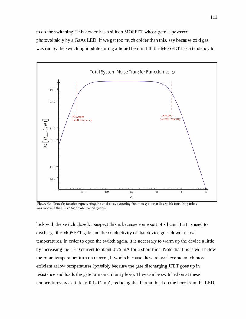
111
to do the switching. This device has a silicon MOSFET whose gate is powered
photovoltaicly by a GaAs LED. If we get too much colder than this, say because cold gas
was run by the switching module during a liquid helium fill, the MOSFET has a tendency to
lock with the switch closed. I suspect this is because some sort of silicon JFET is used to
discharge the MOSFET gate and the conductivity of that device goes down at low
temperatures. In order to open the switch again, it is necessary to warm up the device a little
by increasing the LED current to about 0.75 mA for a short time. Note that this is well below
the room temperature turn on current, it works because these relays become much more
efficient at low temperatures (possibly because the gate discharging JFET goes up in
resistance and loads the gate turn on circuitry less). They can be switched on at these
temperatures by as little as 0.1-0.2 mA, reducing the thermal load on the bore from the LED

112
and any thermocouple effects induced on the MOSFET switch.
The circuit for the stabilization system is included here in figure 6.5. Naively shutting
off the MOSFET switch is an inconvenient way of running the experiment. This causes a 4.2
hour relaxation to the voltage determined by the aforementioned voltage divider between the
1.5 G resistor in parallel with the switch and the 1410 parasitic resistance across the
capacitor. This sag causes a linear drift in the ring voltage and hence the correction signal. At
the very least the resonance fitting software does not like this; a more serious limitation is
that over several hours, the lock loop would run out of compliance range. This problem can
be solved by simply increasing the voltage on the other side of the opened switch. With some
experimentation, the correct number of “battery units” of the bootstrap voltage vernier can be
found so that the voltage ramp is negligible.
Some things needed to be rearranged when we changed over to the RC system. First,
the ring modulation now needs to be injected at the base of the capacitor which is connected
113
to the 100 ohm sense resistor so that it is not filtered out itself. A series resonant “trap” is
placed here as generally noise is attenuated by the 15 mega-ohm resistor in the feedback
circuit. As this is not present for the modulation now, the RF trap attenuates any noise not at
the ring modulation frequency while still passing the required low RF.
The experiment with the cryogenic RC system in place showed a correction voltage
noise that corresponded to a 5 ppb ring voltage noise. This is a factor of 2 improvement over
the unstabilized system. The fact that we do not see a greater improvement indicates that
there are noise sources other than ring supply noise affecting the system. This includes the
Johnson noise of the front end tuned circuit and preamplifier.
Section VI.3: Helium Pressure and Level system
When the single data-point precision of the experiment reached a few parts in 1010
the helium level and pressure systems needed rethinking. In figure 6.6 there is a plot of the
magnetic field change (observed through the cyclotron resonance) as a weather system
passed through Seattle. By this time, liquid helium level locking and bore pressure control
systems had been in place for several years – just not in their final forms. Before these
systems were in place, the magnetic field would change by parts per million as weather
changed. After the first crude attempts at locking up these two quantities, there were still 3
ppb diurnal field changes. The variation in figure 6.6 came from a simple leak in the pressure
reference. The final system, when in place, showed no magnetic field drift with pressure
changes. This system was instrumental in making 3 week measurements of the quality
presented here. The problem was that as the pressure over the liquid helium varied, so did the
temperature of the boiling point of the liquid in the magnet bore tube. The bore tube’s G-10
epoxy-glass composite has a magnetic permittivity that changes as 1
T so at 4.2K its
temperature coefficient becomes rather large. And as the magnetic permittivity of the bore
material changes, so does the field in the bore. This system, designed by P.B. Schwinberg, is
critical to obtaining high accuracy, so I thought it would be good to give a short description
of it.
First, there are two things that need to be controlled, the helium level, and the
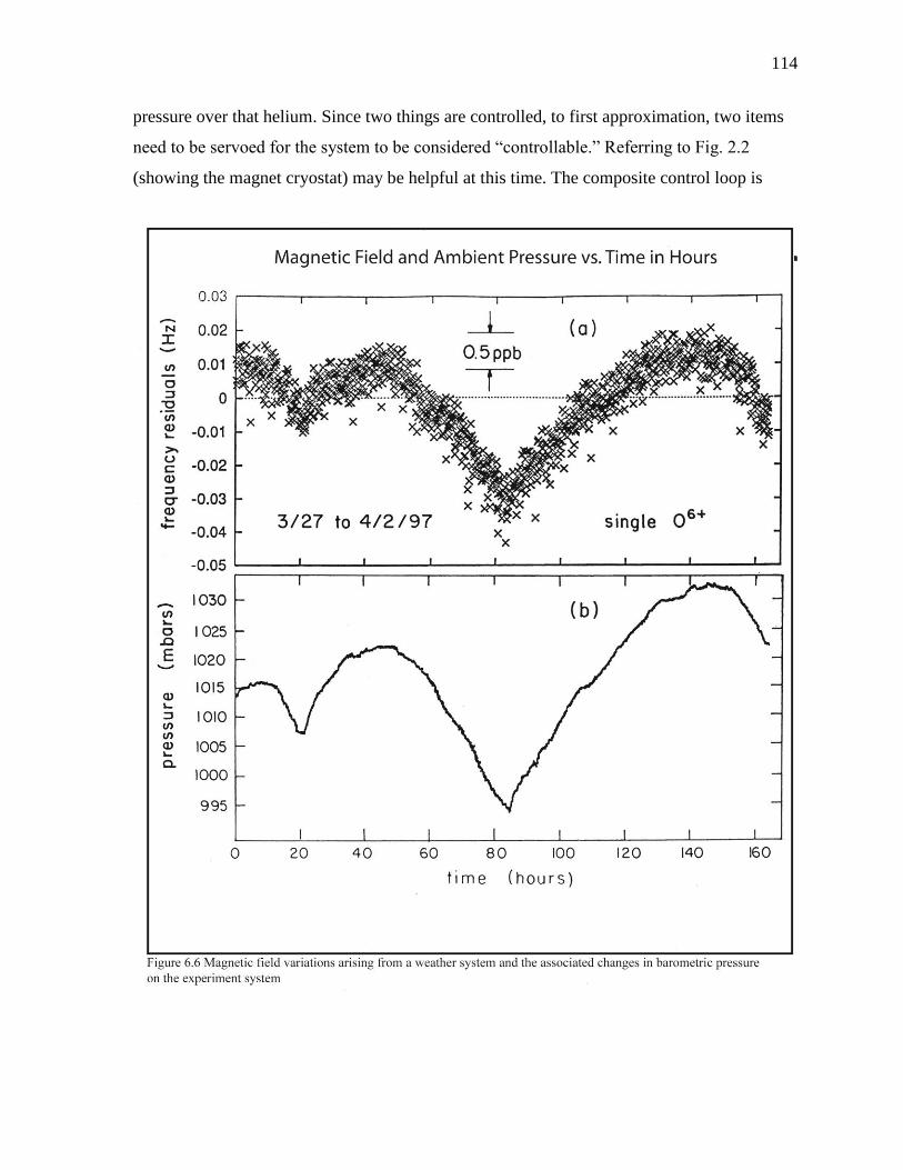
114
pressure over that helium. Since two things are controlled, to first approximation, two items
need to be servoed for the system to be considered “controllable.” Referring to Fig. 2.2
(showing the magnet cryostat) may be helpful at this time. The composite control loop is
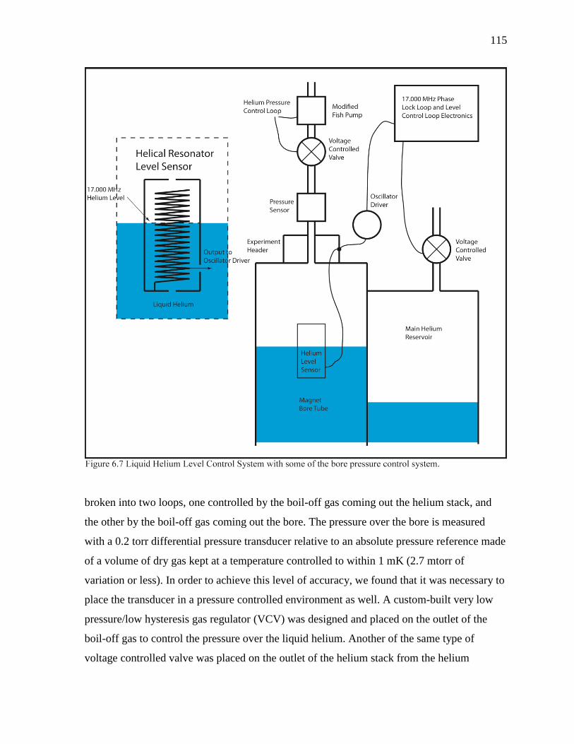
115
broken into two loops, one controlled by the boil-off gas coming out the helium stack, and
the other by the boil-off gas coming out the bore. The pressure over the bore is measured
with a 0.2 torr differential pressure transducer relative to an absolute pressure reference made
of a volume of dry gas kept at a temperature controlled to within 1 mK (2.7 mtorr of
variation or less). In order to achieve this level of accuracy, we found that it was necessary to
place the transducer in a pressure controlled environment as well. A custom-built very low
pressure/low hysteresis gas regulator (VCV) was designed and placed on the outlet of the
boil-off gas to control the pressure over the liquid helium. Another of the same type of
voltage controlled valve was placed on the outlet of the helium stack from the helium

116
reservoir. To keep the two loops from becoming degenerate and strongly coupled, the loop
time constants were kept at least a factor of 10 different.
Though the voltage controlled valve design and use are somewhat novel, this loop is
simply an off the shelf sensor and transducer connected up in a PI (proportional, integrator)
loop with a widely variable gain and time constant. Note the PI design was largely chosen
over the popular PID (proportional, integrator, differentiator) design because it is more easily
controlled with a few knobs (just gain and time constant). For a given number of control loop
parameters to be varied, it provided the most versatility. It is the level sensor and level loop
that I find to be most intriguing, and therefore I will describe it in a little more detail. A
sketch of the main features of the helium liquid level loop is shown in figure 6.7.
When the need for level control first came about, the standard for liquid helium level
sensing was the superconducting sensor. A superconducting sensor is a length of
superconducting wire sent down the liquid helium column. The wire that was under the
helium level went superconducting and the part above the liquid stayed normal. A current
was passed through the wire, and the voltage across the wire is crudely proportional to the
distance above the liquid helium. This sensor method requires, comparatively, a great deal of
power and since liquid helium is relatively expensive, it is not to be wasted (additionally, this
would limit the magnet hold time between fills and therefore experimental run duration.)
Capacitative sensors formed by making an RC-relaxation oscillator out of a pair of parallel
plates submerged in liquid nitrogen are commonplace. These burned far less heat in the
liquid, but the dielectric constant of liquid helium is much less than that of liquid nitrogen so
these capacitive sensors are not very accurate for helium cryogens.
Early in the incorporation of helical resonators in the experiment, it was discovered
that their frequency varied as the liquid level went over them. For example, our 3 inch long
helical resonator at 17 MHz varied by 300 kHz with liquid helium covering its length. P.B.
Schwinberg realized that he could make this into an LC oscillator-detector which can be
more stable than its low frequency RC cousin and would allow capacitive level sensing. This
also increased the detection bandwidth and decreased thermal coupling of the sensing process
to the liquid level, allowing for better control.
The oscillator driver circuit is shown in figure 6.8. It essentially makes a hybrid
Colpitts oscillator with the low impedance node exported out to the helical resonator in the

117
magnet bore with coaxial cable. The active component (dual-gate MOSFET) is not kept in
the bore because it burns roughly 75 times the amount of power as the cryogenic part of the
experiment and so would cause a significant increase in helium boil-off, as well as thermal
instability at the liquid/gas interface. The cable distance is kept well under 8
so that cable
effects are small. The transconductance of the MOSFET is varied by changing the voltage on
the cascode transistor gate so that the circuit is on the verge of oscillating at room
temperature. This is done because marginal oscillators are the most stable. As the
temperature of the resonator goes down, the conductivity of its copper goes up and both its Q
and impedance go up:
_ .TC TC turns ratio
LR Q
C (6.8)
As the losses in the resonator node go down, the circuit starts oscillating. The turns ratio is
kept low (lower impedance) for two reasons. First, impedances in helical resonators are high
compared to the resonator in the driver electronics. And second, if the impedance is very
high, you would be looking more at the unterminated line than the resonator. A target turns
ratio for the transformer would produce a cryogenic impedance of several hundred ohms.
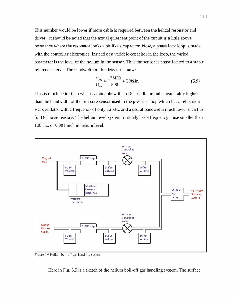
118
This number would be lower if more cable is required between the helical resonator and
driver. It should be noted that the actual quiescent point of the circuit is a little above
resonance where the resonator looks a bit like a capacitor. Now, a phase lock loop is made
with the controller electronics. Instead of a variable capacitor in the loop, the varied
parameter is the level of the helium in the sensor. Thus the sensor is phase locked to a stable
reference signal. The bandwidth of the detector is now:
17
30 .500
res
res
MHzkHz
Q
(6.9)
This is much better than what is attainable with an RC oscillator and considerably higher
than the bandwidth of the pressure sensor used in the pressure loop which has a relaxation
RC-oscillator with a frequency of only 12 kHz and a useful bandwidth much lower than this
for DC noise reasons. The helium level system routinely has a frequency noise smaller than
100 Hz, or 0.001 inch in helium level.
Here in Fig. 6.9 is a sketch of the helium boil-off gas handling system. The surface
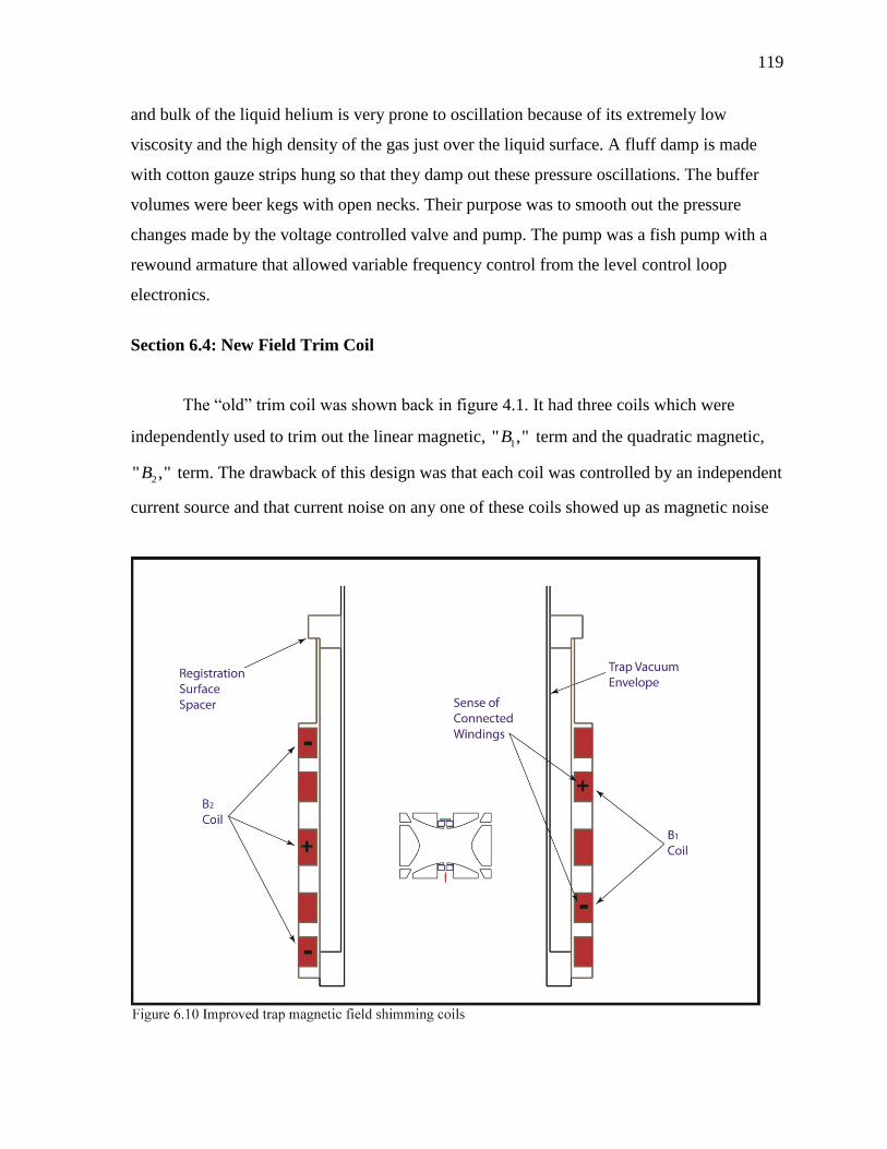
119
and bulk of the liquid helium is very prone to oscillation because of its extremely low
viscosity and the high density of the gas just over the liquid surface. A fluff damp is made
with cotton gauze strips hung so that they damp out these pressure oscillations. The buffer
volumes were beer kegs with open necks. Their purpose was to smooth out the pressure
changes made by the voltage controlled valve and pump. The pump was a fish pump with a
rewound armature that allowed variable frequency control from the level control loop
electronics.
Section 6.4: New Field Trim Coil
The “old” trim coil was shown back in figure 4.1. It had three coils which were
independently used to trim out the linear magnetic, 1" ,"B term and the quadratic magnetic,
2" ,"B term. The drawback of this design was that each coil was controlled by an independent
current source and that current noise on any one of these coils showed up as magnetic noise

120
seen by the particle. This was simple and provided the uniform magnetic field changes
needed for the original “variable bottle” [43] experiments. The old design was used for all the
data taken at UW. An improved design was constructed for the new double trap experiment
which is now in Germany.
The improved design is shown in figure 6.10. It groups 5 coils into two orthogonal
coils, each with a nulled uniform magnetic “ 0 ,B ” term. Each group is connected together
with the winding senses as shown in the figure. A 1B coil produces a linear gradient to shim
away the effect of any residual linear magnetic gradient caused by trap parts. This term
would interact with the experiment by changing any difference in particle position to a field
difference, and therefore a cyclotron frequency difference that is not related to a mass
change. A 2B coil introduces an anharmonic term to couple the particle’s orbit radius to its
axial frequency. By switching to an orthogonal coil system, to the degree that the 0B term is
nulled out for each coil, the effect of current noise on the field that the particle sees is
reduced. This greatly relaxes the current driver stability criterion. Since we no longer do
experiments with the “variable bottle” [43], a 0B coil is now redundant, though it could have
been incorporated into the design. The new design is not without cost. In order to fit around
the new, larger, trap envelope and to be removable for a high temperature bake-out, the
radius of the coils needed to be larger. The 1B term has a 2
1
r strength dependence and the the
2B term has a 3
1
r strength dependence, requiring four and eight times as many turns to
produce the same gradients. Since copper’s resistance largely drops away at liquid helium
temperatures, the extra copper only provided an additional spatial constraint.
Section 6.5: Helical Resonator Coil Trimming Circuit
In the concluding sections, I will present several circuits that proved useful in the
experiments done after the deuterium data was taken. I am selecting ones that include an
unusual technique that someone trying to repeat this experiment might like to know.

121
The first circuit is shown in figure 6.11. It is used with the helical resonator to tune it over a
narrow range. This is useful because the tuned circuit characteristics change slightly with
time, especially as the front end FETs age. The particle must be kept close to the peak of the
tuned circuit so an extra phase is not picked up here. The GaAs varactors have Q’s in excess
of 5000 at 50 MHz at room temperature. It is likely they are better at cryogenic
temperatures, however, this is not necessarily so as their carrier mobility goes up and
therefore their operating point changes considerably. At the very least, their operating range
decreases. Since we only want a narrow tuning range, they are tapped down on the resonator
to a point where the effective capacitance is large. Note that large resistors are necessary in
the feed network to both isolate the tuned circuit from noise from external electronics and to
isolate the resonator from the 50 ohm line feeding the varactor. The capacitors are of the NP0
(Negative, Positive, Zero) type for reasons of both high Q and stability of the dielectric at
low temperatures. Note also that the amplifier’s optimal tap point may not be at the top of the

122
resonator where the particle is coupled to it. This is to reduce the effect of current noise from
the preamplifier. The back-to-back limiting diodes are not included in this figure for clarity.
Section 6.6: High Voltage Current Limiter
Fig. 6.12 is a 12 nanoamp limiting circuit for the ion loading electron source. This is
useful for two reasons. The first is that field emission points (FEPs) are fragile. If one
accidently puts on too much voltage, they will pass more current than is best. While they are
repelling the electrons flowing from their tip, they are attracting positive ions which impact
and destroy them. As the background gas pressure is extremely low, the damage is not as bad
as it could be; however, the tips do age from this effect. Keeping the tips at low current
prevents the need to remove the tip to re-etch it to a sharp point. The second reason is to limit
the current in case of high-voltage breakdown of the cable in the liquid helium. If unchecked,
this arc can put down a conductive trace of carbon which renders the FEP line useless.
Limiting the current to nanoamps makes it so that there is not enough power in the break-
down arc to ionize the cable insulation.

123
This circuit replaced gigaohm resistors placed in series with the line at the experiment
header. While these reduced the chance of pulling too much current from the FEP, they did
not do so very effectively and they did not prevent an over-voltage arc from forming as that
would bypass the limiting resistor. The main trick to this circuit is to use a high voltage IGBT
or MOSFET to extend the voltage range of a JFET current source. The JFET circuit alone
works well, but cannot exceed 40 volts before it breaks down. By placing a high voltage
device in series with it, and using a 9 volt battery to bias its gate, the voltage range was
extended beyond 1200 V. At that point the leakage current from the drain to the gate started
pulling extra current through the device, though it still performed well as a limiter. High
voltage destructive testing was never performed, though it was tested safely to 1500 volts.
Less than 3 volts were dropped in the device when it was not limiting, allowing precision
control of the FEP current. The high voltage diode is included to protect the circuit from
being hooked up in reverse. In general, however, it does not provide nanoampere protection
in reverse bias because of the limitations of high voltage diodes.
Section 6.7: 100 kHz Multiband Amplifier
Figure 6.13 shows the schematic for a dual bandwidth 100 kHz amplifier used on the
100 kHz IF. It provides two output levels with an adjustable gain in two bandwidths. The
narrow band is used for general experiment running. The wide band circuit is used to
measure the front end tuned circuit profile with an RMS noise detector (direct excitation of
the tuned circuit is not allowed with a particle in the trap as this would directly drive the
particle’s axial motion and possibly expel the particle from the trap).
The main reason to show this circuit is to familiarize the reader with crystal filter
circuit design. The crystal is a 100 kHz series tuned quartz crystal made by International
Crystal Manufacturing. The tuned transformer input and output couple energy more
efficiently into and out of the device. The higher the impedance, the wider the crystal filter is.
Usually, we want the narrowest filter possible; however, below a certain point the crystal is
limited by its intrinsic Q and the only result of going lower in impedance is to increase the
filters insertion loss. The 18 pF capacitor at the opposite polarity of the transformer cancels
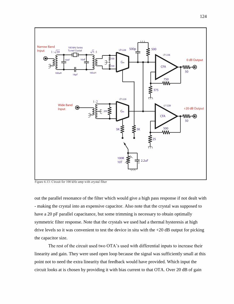
124
out the parallel resonance of the filter which would give a high pass response if not dealt with
- making the crystal into an expensive capacitor. Also note that the crystal was supposed to
have a 20 pF parallel capacitance, but some trimming is necessary to obtain optimally
symmetric filter response. Note that the crystals we used had a thermal hysteresis at high
drive levels so it was convenient to test the device in situ with the +20 dB output for picking
the capacitor size.
The rest of the circuit used two OTA’s used with differential inputs to increase their
linearity and gain. They were used open loop because the signal was sufficiently small at this
point not to need the extra linearity that feedback would have provided. Which input the
circuit looks at is chosen by providing it with bias current to that OTA. Over 20 dB of gain
125
adjustment was available by varying this bias current. Since there was an additional CFA
already in the two packages used, I wired it up to produce an alternate output level. Both
CFA’s are mirroring the same signal. The 50 ohm resistor on the output is for transmission
line termination; it is also beneficial if the next stage is transformer coupled. Under
circumstances where these things are not a concern, the resistor could be omitted. I rolled off
the gain of the device at 600 kHz so that they did not pass unnecessary frequencies. Note that
this 500 pF capacitor should be of the NP0 or plastic film type so that the phase of the
amplifier does not change with temperature. Note also that a more elaborate network could
have been used here, including a LC tank with a limiting resistor, but was deemed
unnecessary.

126
Bibliography
[1] F. M. Penning, "Die Glimmentlaudung Bei Niedrigen Druck Zwischen Koaxialen
Zylindern in einem Axialen Magnetfeld," Physica, vol. III, no. 9, pp. 873-894.
[2] R. S. Van Dyck Jr., P. Schwinberg and H. Dehmelt, "Precise Measurements of Axial,
Magnetron, Cyclotron, and Spin-Cyclotron-Beat Frequencies on an isolated 1-meV
Electron," Physical Review Letters, vol. 38, no. 7, pp. 310-314, 1977.
[3] P. B. Schwinberg, R. S. Van Dyck Jr. and H. G. Dehmelt, "New Comparison of the
Positron and Electron g Factors," Physical Review Letters, vol. 47, no. 24, pp. 1679-
1682, 1981.
[4] H. G. Dehmelt, "Spin resonance of Free Electrons Polarized by Exchange Collisions,"
Physical Review, vol. 2, pp. 381-385, 1958.
[5] R. S. V. D. Jr., D. J. Wineland, P. A. Ekstrom and H. G. Dehmelt, "High Mass
Resolution with a New Variable Anharmonicity Penning Trap," Applied Physics Letters,
vol. 28, no. 8, pp. 446-448, 1976.
[6] R. S. Van Dyck Jr., F. Moore, D. Farnham and P. Schwinberg, Bull. Am. Phys. Soc, vol.
31, p. 244, 1986.
[7] R. S. V. D. Jr., F. L. Moore, D. L. Farnham and P. B. Schwinberg, "Mass Ratio
Spectroscopy and the Proton's Atomic Mass," in Frequency Standards and Metrology,
Heidleberg, 1989.
[8] R. S. Van Dyck Jr., D. Farnham and P. Schwinberg, Physica Scripta, vol. T59, p. 134,
1995.
[9] R. S. Van Dyck Jr., D. Farnham and P. Schwinberg, "A compensated Penning Trap
Mass Spectrometer and the H(3)-He(3) Mass Difference," Jounrnal of Modern Optics,
vol. 39, no. 2, pp. 243-255, 1992.
[10] R. S. Van Dyck Jr., D. Farnham and P. Schwinberg, "High Precision Penning Trap Mass
Spectroscopy of the Light Ions," in 9th Int. Conf. on Atomic Masses and Fundamental
Constants, Bernkastel-Kues, 1992.
[11] D. L. Farnham, R. S. J. Van Dyck and P. B. Schwinberg, "Determination of the
Electron's Atomic Mass and the Proton/Electron Mass Ratio via Penning Trap Mass
Spectroscopy," Physical Review Letters, vol. 75, no. 20, pp. 3598-3601, 1995.
[12] D. B. Pinegar, K. Blaum, T. P. Biesiadzinski, S. L. Zafonte and R. S. Van Dyck Jr.,
"Stable Voltage Source for Penning Trap Experiments," Review of Scientific
Instruments, vol. 80, pp. 064701/1-8, 2009.
[13] K. Blaum, Y. N. Novikov and G. Werth, "Penning Traps as a Versatile Tool for Precise
Experiments in Fundamental Physics," Contemporary Physics, vol. 51, no. 2, pp. 149-
175, 2010.
[14] C. Diehl, K. Blaum, M. Hocker, J. Ketter, D. B. Pinegar, S. Streubel and R. S. Van Dyck
Jr., "Progress with the MPIK/UW-PTMS in Heidelberg," Hyperfine Interactions, vol.
199, pp. 291-300, 2011.
[15] J. K. Thompson, S. Rainville and D. E. Pritchard, "Cyclotron Frequency Shifts Arising
from Polarization Forces," Nature, vol. 430, pp. 58-61, 2004.
[16] S. Rainville, J. Thompson, E. Meyers, B. J.M., M. Dewey, E. Kessler, R. Deslattes, H.

127
Borner, M. Jentsche and D. Pritchard, "A Direct Test of E=mc^2," Nature, vol. 438, no.
22/29, pp. 1096-1097, 2005.
[17] B. J. Mount, M. Redshaw and E. Myers, "Atomic Masses of (6)Li, (23)Na, (39.41)K,
(85,87)Rb, and (133)Cs," Physical Review A, vol. 82, no. 4, pp. 042513/1-5, 2010.
[18] B. J. Mount, M. Redshaw and E. Meyers, "Q Value of (115)In->(115)Sn(3/2+): The
Lowest Known Energy Beta-Decay," Physical Review Letters, vol. 103, no. 12, pp.
122502/1-4, 2009.
[19] M. Redshaw, B. Mount, E. Meyers and F. I. Avignone, "Masses of (130)Te and (130)Xe
and Double-Beta-Decay Q Value of (130)Te," Physical Review Letters, vol. 102, no. 21,
pp. 212502/1-4, 2009.
[20] A. Solders, I. Bergstrom, S. Nagy, M. Suhowen and R. Schuch, "Determination of the
Proton Mass From a Measurement of the Cyclotron Frequencies of D+ and H2+ in a
Penning Trap," Physical Review A, vol. 78, no. 1, pp. 012514/1-6, 2008.
[21] R. S. Van Dyck Jr., D. Farnham, S. Zafonte and P. Schwinberg, "Ultrastable
Superconducting Magnet System for a Penning Trap Mass Spectrometer," Review of
Scientific Instruments, vol. 70, no. 3, pp. 1665-1671, 1999.
[22] E. G. Kessler Jr., M. Dewey, R. Deslattes, A. Henins, H. Borner, M. Jentschel, C. Doll
and H. Lehmann, "The Deuteron Binding Energy and the Neutron Mass," Phs. Lett. A,
vol. 255, pp. 221-229, 1999.
[23] V. Natarajan, K. R. Boyce, F. DiFilippo and D. E. Pritchard, "Precisiion Penning Trap
Comparison of Non-doublets: Atomic Masses of H, D, and the Neutron," Physical
Review Letters, vol. 71, no. 3, pp. 1998-2001, 1993.
[24] B. Odom, D. Nanneke, B. D'Urso and G. Gabrielse, "New Measurement of the Electron
Magnetic Moment Using a One-Electron Quantum Cyclotron," Physical Review Letters,
vol. 97, pp. 030801/1-4, 2006.
[25] G. G. Lowell S. Brown, "Geonium Theory: Physics of a Single Electron or Ion in a
Penning Trap," Reviews of Modern Physics, vol. 58, no. 1, pp. 233-312, 1986.
[26] J. M. Lockhart, R. L. Fagaly, L. W. Lombardo and B. Muhlfelder, "Magnetic
Susceptibility of Instrument Materials Below 10K," Physica B, vol. 165 & 166, pp. 147-
148, 1990.
[27] G. Gabrielse and J. Tan, "Self Shielding Superconducting Solenoid Systems," Journal of
Applied Physics, vol. 63, no. 10, pp. 5143-5148, 1988.
[28] A. van der Ziel, "Gate noise in field effect transistors at moderately high freuency,"
Proceedings of IEEE, vol. 51, no. 3, pp. 952-953, June 1963.
[29] E. W. Kirk, A. van der Ziel, E. Chenette and C. Kim, "Induced gate noise in
MOSFETs," Solid State Electronics, vol. 14, no. 10, pp. 945-948, 1971.
[30] A. Pawlikiewicz and A. van der Ziel, "Induced Gate 1/f Noise in MODFETs in the Low
GHz Range," Solid State Electronics, vol. 29, no. 3, pp. 379-380, 1986.
[31] R. S. Van Dyck Jr., D. P. Pinegar, S. Van Liew and S. L. Zafonte, "The UW-PTMS,
Systematic Studies, Measurement Progress, and Future Improvements," International
Journal of Mass Spectroscopy, vol. 251, pp. 231-242, 2006.
[32] R. S. Van Dyck Jr., F. Moore, D. Farnham, P. Schwinberg and H. Dehmelt,
"Microwave-cavity Modes Directly Observed in a Penning Trap," Physical Review A,

128
vol. 36, no. 7, pp. 3455-3456, 1 October 1987.
[33] R. S. Van Dyck Jr., P. B. Schwinberg and H. G. Dehmelt, "Electron Magnetic Moment
from Geonium Spectra," in New Frontiers in High-Energy PHysics, Coral Gables,
Florida, 1978.
[34] D. Farnham, "A Determination of the Electron/Proton Mass Ratio and the Electron's
Atomic Mass via Penning Trap Mass Spectroscopy: A Thesis," University of
Washington, Seattle, Washington, 1995.
[35] R. S. Van Dyck Jr., D. Farnham and P. Schwinberg, "Progress on the H(3)-He(3) Mass
Difference Using the Compensated Penning Trap Spectrometer," Physica Scripta, vol.
46, pp. 257-263, 1992.
[36] R. S. Van Dyck Jr., F. Moore, D. Farnham and P. Schwinberg, "Number Dependency in
the Compensated Penning Trap," Physical Review A, vol. 40, no. 11, pp. 6308-6313,
1989.
[37] J. Porto, "Series Solution for the Image Charge Fields in Arbitrary Cylindrical Penning
Traps," Physical Review A, vol. 64, no. 2, pp. 023403/1-7, 2001.
[38] J. B. Jeffries, S. Barlow and G. Dunn, "Theory of Space-Charge Shift of Ion Cyclotron
Resonance Frequencies," International Journal of Mass Spectrometry and Ion
Processes, vol. 54, pp. 169-187, 1983.
[39] D. J. Wineland, W. M. Itano and R. Van Dyck Jr., "High-Resolution Spectroscopy of
Stored Ions," Advances in Atomic and Molecular PHysics, vol. 19, pp. 135-186, 1983.
[40] W. H. Greene, Econometric Analysis, New York: Macmillan Publishing Company,
1993.
[41] P. E. Gill and W. Murray, "Algorithms for the Solution of the Non-Linear Least Squares
Problem," SIAM Journal on Numerical Analysis, vol. 15, no. 5, pp. 977-992, 1978.
[42] CODATA and NIST, "CODATA Recommended Values of the Fundamental Physical
Constants: 2010," NIST, 2011.
[43] R. S. Van Dyck Jr., F. Moore, D. Farnham and P. Schwinberg, "Variable Magnetic
Bottle for Precision Geonium Experiments," Review of Scientific Instruments, vol. 57,
no. 4, pp. 593-597, 1986.
[44] R. S. Van Dyck Jr., D. Farnham and P. Schwinberg, "Proton-Electron Mass Ratio and
the Electron's "Atomic Mass"," IEEE Transactions on Instrumentation and Measuremt,
vol. 44, no. 2, 1995.
[45] R. S. Van Dyck Jr., D. Farnham, S. Zafonte and P. Schwinberg, "High Precision
Penning Trap Mass Spectroscopy and a New Measurement of the Proton's "Atomic
Mass"," in Trapped Charged Particles and Fundamental Physics, Monterey, 1999.
[46] G. Audi, A. H. Wapstra and C. Thibault, "The Ame2003 Atomic Mass Evaluation (II),"
Nuclear Physics, vol. A729, pp. 337-676, 2003.

129
Appendix A: Experimental Parameters
Table A.1 Experimental Parameters
Description Symbol Value
Trap Frequencies
Cyclotron, Deuteron (MHz) ,c D 44.974
Cyclotron, Carbon 6+ (MHz) , 6c C 45.293
Cyclotron, Carbon 4+ (MHz) , 4c C 30.075
Axial, typ. (MHz) z 3.56
Magnetron, Deuteron (MHz) ,m D
0.141
Magnetron, Carbon 6+ (MHz) , 6m C
0.140
Magnetron, Carbon 4+ (MHz) , 4m C
0.211
Axial Linewidth, Deuteron (mHz) ,z D 85
Axial Linewidth, Carbon 6+ (mHz) , 6z C 510
Axial Linewidth, Carbon 4+ (mHz) , 4z C 215
Trap Parameters
Minimum Ring Electrode Inner Radius (mm) 0 2.74
Minimum Endcap Spacing to Trap Center (mm) 0z 2.28
Trap Characteristic Dimension (mm) d 2.11
Ring Voltage, Deuteron (V) ,ring DV
-46.93
Ring Voltage, Carbon 6+ (V) , 6ring CV
-46.62
Ring Voltage, Carbon 4+ (V) , 4ring CV
-69.93
Magnetic Bottle, Run #1 to Run #12 ( 2G cm ) 2B 0.569(65)
Magnetic Bottle, Run #13 and Run #14 ( 2G cm ) 2B 1.702(107)
Minimum 4C - 610 4,minC 2.8
Residual Energies
Residual Magnetron Energy (meV) ,m resE 0.06(2)
Residual Axial Energy (meV) ,z resE 0.91(55)
Residual Cyclotron Energy (meV) ,c resE 30(20)

130
Appendix B: Data Analysis Code
The code in this appendix will not win any beauty contests, but it is provided so that the
results in this dissertation can be more easily repeated. The first program is the data fit
supervisor for the model quadratic in time called “fit_data”:
%% fit_data %% Comment Section % ############################################################## % This is the super-routine that is called to fit the data. % Other scripts are called inside it % Variables Used: % numpoints_ion1 % numpoints_ion2 % data_count % typ_sigma_ion_1 % typ_sigma_ion_2 % ############################################################## %% Set problem scale factors clear all; scale_factor=3.3e7; lsc=.01; qsc=.0001; %% Load and prepare data based on the data written in write_run_params prepare_runs; %% Provide the fitting routine with the initial guess q_initial_guess; %% Data fit loop cont='y'; % Full speed ahead iter=1; step_size(iter)=10^10; % Set a step so big it can't be worse while cont=='y' q_hess_jacob; % Compute hessian and jacobian of
objective fnx del_beta=hess\jaco; % Get delta to new guess guess=guess-del_beta; % Get new guess iter=iter+1; step_size(iter)=norm(del_beta,2); % Check to see if we are
improving if step_size(iter-1)<step_size(iter) % If not improving, pause and
plot subplot(1,2,2); plot_residuals; % Plot residuals, model, fit
quality cont=input('Another iteration (y/n)? -->','s'); % Ask to proceed end end % Loop on continue %% Run final hessian %qmodel_hess_jacob; q_hess_jacob; %% Compute Standard Errors Inv_Hess=inv(hess); % Compute covariance matrix chi_squ=0;
131
for i=1:data_count; param_sum=0; k=1; while k<=param_measd param_sum=param_sum+guess(4+k)*data(i,2+k); k=k+1; end if data(i,1)<0 model_i=scale_factor*guess(1)*(1-guess(2))...
*(1+data(i,1)*(guess(3)*lsc+data(i,1)*guess(4)*qsc)+param_sum); else model_i=scale_factor*guess(1)*(1+guess(2))...
*(1+data(i,1)*(guess(3)*lsc+data(i,1)*guess(4)*qsc)+param_sum); end chi_squ=chi_squ+(data(i,2)-model_i)^2/(data_sigma(i)^2); end chi_squ=chi_squ/(data_count-4-param_measd); chi=sqrt(chi_squ); Sigma=zeros(param_measd+4,1); for j=1:(param_measd+4) Sigma(j)=sqrt(Inv_Hess(j,j)); end %% Compute Final Point per Point Sigmas countA=0; countB=0; chiA=0; chiB=0; for i=1:data_count; param_sum=0; k=1; while k<=param_measd param_sum=param_sum+guess(4+k)*data(i,2+k); k=k+1; end if data(i,1)<0 countA=countA+1; model_i=scale_factor*guess(1)*(1-guess(2))*(1+data(i,1)... *(guess(3)*lsc+data(i,1)*guess(4)*qsc)+param_sum); resA(countA)=(data(i,2)-model_i); chiA=chiA+resA(countA)^2; else countB=countB+1; model_i=scale_factor*guess(1)*(1+guess(2))*(1+data(i,1)... *(guess(3)*lsc+data(i,1)*guess(4)*qsc)+param_sum); resB(countB)=(data(i,2)-model_i); chiB=chiB+resB(countB)^2; end end chiA=chiA/(countA-4-param_measd); sigA=quantile(abs(resA),.683); chiB=chiB/(countB-4-param_measd); sigB=quantile(abs(resB),.683); %% Plot Final Data plot_residuals; ion1_scale=typ_sigma_2/typ_sigma_1;

132
Scaled_residuals=Residuals; for i=1:numpoints_ion1 % scale deuterium data for normplot Scaled_residuals(i)=Scaled_residuals(i)*ion1_scale; end subplot(1,2,1); normplot(Scaled_residuals); %% Print parameters about final data fit fprintf('Overal Multiplier = %.12e\tsigma = %e\n',guess(1),Sigma(1)*chi); fprintf('Step Multiplier = %.12e\tsigma = %e\n',guess(2),Sigma(2)*chi); fprintf('Linear Coef = %.10e\tsigma = %e\n',guess(3),Sigma(3)*chi); fprintf('Quadratic Coef = %.10e\tsigma = %e\n',guess(4),Sigma(4)*chi); for j=5:(param_measd+4) fprintf('Param(%u)=%.12e\tsigma(%u)=%e\n',j-4,guess(j),j-
4,Sigma(j)*chi); end cfr=(1-guess(2))/(1+guess(2)); cfr_sigma=cfr*Sigma(2)*(1/(1-guess(2))+1/(1+guess(2))); if chg_2==6 fprintf('CFR = 992 996 654 %.3f\t+/- %.3f ppt\n',... 10^12*(cfr-.992996654),10^12*cfr_sigma*chi); else fprintf('CFR = 1 489 631 086 %.3f\t+/- %.3f ppt\n',... 10^12*(cfr-1.489631086),10^12*cfr_sigma*chi); end fprintf('Reduced sqrt(Chi Squared) =%f\n',chi); fprintf('Scatter for ion A %e\n',sigA); % Print out point2point
scatters fprintf('Scatter for ion B %e\n',sigB); %% Calculate and print traditional covariance matrix quantities qmodel_hess_cov; fprintf('Traditional error %.3f ppt\n',... 1e12*chi*sqrt(cov_mat(2,2))*cfr*(1/(1-guess(2))+1/(1+guess(2)))); %% End of script
The second code excerpt is a script called by the supervisor: “prepare_runs”
%% Intro Comments % prepare_runs % ##################################################################### % This script concatenates two data runs to one data set % 1)The hours are changed so that hour 0 is at the beginning % of run #2. % 2)The fcp offset is changed to fcp, then to the free space % number, fc. % 3)The sigma is replaced by the maximum of the f-file sigma % and the chosen minimum sigma from run_params file. % 4)Only the parameters to be used are kept and their number % is counted. % 5)The number of data points are counted % Variables used: % Variables created available for future: % param_count % param_measd % numpoints_ion1 % numpoints_ion2

133
% data_count % data_cache_1 % data_cache_2 % data % data_sigma % Variables imported: % a bunch % ##################################################################### %% Declare Constants params=zeros(5,1); imagech_cor=0.00223; % Image charge shift per charge on
ion range_cor=0.0291; % Range effect cor in Hz/Hz %% Choose and Load run_params file to specify data to use
[run_params_file,data_dir]=uigetfile('run_params_*','Find Run
Configuration File'); fid_params=fopen(fullfile(data_dir,run_params_file));
% Ion 1 parameters data_dir=fscanf(fid_params,'%s ',1); % Read data directory data_file1=fscanf(fid_params,'%s ',1); % Read name of data file 1 ion1_begin=fscanf(fid_params,'%f',1); % Read first hour of ion 1 run ion1_end=fscanf(fid_params,'%f',1); % Read last hour of ion 1 run
offset_fcp1=fscanf(fid_params,'%f',1); % Read fcp offset for ion 1 fz_1=fscanf(fid_params,'%f',1); % Read fz for ion 1 fm_1=fscanf(fid_params,'%f',1); % Read fm for ion 1 typ_sigma_1=fscanf(fid_params,'%f',1); % Read typical sigma for ion 1 max_sigma_1=fscanf(fid_params,'%f',1); % Read maximum allowed sigma for
ion 1 offset_fzpwr1=fscanf(fid_params,'%f',1);% Read axial power offset for ion
1 lnwdth_1=fscanf(fid_params,'%f',1); % Read axial linewidth of ion 1 phase_1=fscanf(fid_params,'%f',1); % Read set phase lead of ion 1 phase_1=phase_1*(2*pi/360); % Change phase to radians chg_1=fscanf(fid_params,'%u',1); % Read Charge of ion 1 rng_1=fscanf(fid_params,'%f',1); % Read sweep range of ion 1
% Ion 2 parameters data_dir=fscanf(fid_params,'%s ',1); % Read data directory data_file2=fscanf(fid_params,'%s ',1); % Read name of data file 2 ion2_begin=fscanf(fid_params,'%f',1); % Read first hour of ion 2 run ion2_end=fscanf(fid_params,'%f',1); % Read last hour of ion 2 run
offset_fcp2=fscanf(fid_params,'%f',1); % Read fcp offset for ion 2 fz_2=fscanf(fid_params,'%f',1); % Read fz for ion 2 fm_2=fscanf(fid_params,'%f',1); % Read fm for ion 2 typ_sigma_2=fscanf(fid_params,'%f',1); % Read typical sigma for ion 2 max_sigma_2=fscanf(fid_params,'%f',1); % Read maximum allowed sigma for
ion 2 offset_fzpwr2=fscanf(fid_params,'%f',1);% Read axial power offset for ion
2 lnwdth_2=fscanf(fid_params,'%f',1); % Read axial linewidth of ion 2 phase_2=fscanf(fid_params,'%f',1); % Read set phase lead of ion 2 phase_2=phase_2*(2*pi/360); % Change phase to radians

134
chg_2=fscanf(fid_params,'%u',1); % Read Charge of ion 2 rng_2=fscanf(fid_params,'%f',1); % Read sweep range of ion 2
% Run parameters zero_hour=fscanf(fid_params,'%f',1); % Read zero hour params=fscanf(fid_params,'%i',5); % Read vector of parameters to use
in fit params_fixed=fscanf(fid_params,'%i',5); % Read vector of parameters to
fix in fit c_fixed=zeros(5,1); for i=1:5 if params_fixed(i)==1 c_fixed(i)=fscanf(fid_params,'%f',1); % Read the i-1th fixed
coefficient end end fclose(fid_params); % Close run params file
%% Read ion 1&2 data files into program, preen and adjust data fid_ion1=fopen(fullfile(data_dir,data_file1)); % Open data file 1 fid_ion2=fopen(fullfile(data_dir,data_file2)); % Open data file 2 data_ion1_raw=textscan(fid_ion1,'%n%n%n%n%n%n%n%n%n','delimiter',',',... 'commentStyle','#','CollectOutput',true); % read data_ion2_raw=textscan(fid_ion2,'%n%n%n%n%n%n%n%n%n','delimiter',',',... 'commentStyle','#','CollectOutput',true); % read fclose(fid_ion1); % Close ion 1 data file fclose(fid_ion2); % Close ion 2 data file data_ion1=data_ion1_raw{1,1}; data_ion2=data_ion2_raw{1,1}; %% Change fcp column to fc data_ion1(:,2)=data_ion1(:,2)+offset_fzpwr1; % Add f_c axial power
offset to ion 1 data_ion2(:,2)=data_ion2(:,2)+offset_fzpwr2; % Add f_c axial power
offset to ion 2 data_ion1(:,2)=data_ion1(:,2)+offset_fcp1; % Add f_c offset to ion 1 data_ion2(:,2)=data_ion2(:,2)+offset_fcp2; % Add f_c offset to ion 2 cp1=data_ion1(1,2); % typical cyclotron for
ion1 cp2=data_ion2(1,2); % typical cyclotron for
ion2 cpcor_1=imagech_cor*chg_1+range_cor*rng_1; % cyc primed corrections cpcor_2=imagech_cor*chg_2+range_cor*rng_2; axcor_1=0.5*lnwdth_1*tan(phase_1); % axial frequency
corrections axcor_2=0.5*lnwdth_2*tan(phase_2); magcor_1=-imagech_cor*chg_1; magcor_2=-imagech_cor*chg_2; data_ion1(:,2)=sqrt((data_ion1(:,2)+cpcor_1).^2 + (fz_1+axcor_1)^2 +
(fm_1+magcor_1)^2); data_ion2(:,2)=sqrt((data_ion2(:,2)+cpcor_2).^2 + (fz_2+axcor_2)^2 +
(fm_2+magcor_2)^2); cyc1=data_ion1(1,2); cyc2=data_ion2(1,2); %% Print corrections out ph_cyc_1=axcor_1*fz_1/offset_fcp1;

135
ph_cyc_2=axcor_2*fz_2/offset_fcp2; ph_run=axcor_1*fz_1/cyc1^2-axcor_2*fz_2/cyc2^2; fprintf('Phase correction for ion #1 is ==> %f mHz\n',1000*ph_cyc_1); fprintf('Phase correction for ion #2 is ==> %f mHz\n',1000*ph_cyc_2); fprintf('Phase correction for RUN is ==> %.2f ppt\n',ph_run*10^12); ran_run=cp1*range_cor*rng_1/cyc1^2-cp2*range_cor*rng_2/cyc2^2; fprintf('Range correction for ion #1 is ==> %f
mHz\n',1000*range_cor*rng_1); fprintf('Range correction for ion #2 is ==> %f
mHz\n',1000*range_cor*rng_2); fprintf('Range correction for RUN is ==> %.2f ppt\n',10^12*ran_run); im_run=cp1*imagech_cor*chg_1/cyc1^2-cp2*imagech_cor*chg_2/cyc2^2; fprintf('Image charge correction for ion #1 is ==> %f mHz\n',... 1000*imagech_cor*chg_1); fprintf('Image charge correction for ion #2 is ==> %f mHz\n',... 1000*imagech_cor*chg_2); fprintf('Image charge correction for RUN is ==> %.2f ppt\n',10^12*im_run); ax_run=cp1*offset_fzpwr1/cyc1^2-cp2*offset_fzpwr2/cyc2^2; fprintf('Axial power correction for ion #1 is ==> %f
mHz\n',1000*offset_fzpwr1); fprintf('Axial power correction for ion #2 is ==> %f
mHz\n',1000*offset_fzpwr2); fprintf('Axial power correction for RUN is ==> %.2f ppt\n',ax_run*10^12); totalcor_1=1000*ph_cyc_1+1000*range_cor*rng_1+... 1000*imagech_cor*chg_1+1000*offset_fzpwr1; totalcor_2=1000*ph_cyc_2+1000*range_cor*rng_2+... 1000*imagech_cor*chg_2+1000*offset_fzpwr2; fprintf('Total correction for ion #1 is ==> %f mHz\n',totalcor_1); fprintf('Total correction for ion #2 is ==> %f mHz\n',totalcor_2); %% Scale data set (frequencies) by scale factor to better condition
hessian matrix %data_ion1(:,2)=data_ion1(:,2)*scale_factor; %data_ion2(:,2)=data_ion2(:,2)*scale_factor; %% Adjust data by sigmas: Throw out bad % Adjust data sigma to min_sigma_1 if less than min allowable for ion #1 numpoints_ion1=size(data_ion1,1); % Throw out data with greater than max allowable sigma, Ion #1 j=1; i=1; for i=numpoints_ion1:-1:1 if data_ion1(i,3) > max_sigma_1 data_ion1(i,:)=[]; end end
numpoints_ion2=size(data_ion2,1); for i=numpoints_ion2:-1:1 if data_ion2(i,3)>max_sigma_2 data_ion2(i,:)=[]; end end %% Adjust data by sigmas: adopt typical sigma of ion for other points data_ion1(:,3)=typ_sigma_1; data_cache_1=data_ion1; data_ion2(:,3)=typ_sigma_2; data_cache_2=data_ion2; % Recount points

136
numpoints_ion1=size(data_cache_1,1); numpoints_ion2=size(data_cache_2,1); %% Determine beginning and end points in run % Ion 1 for i=1:numpoints_ion1 % keep data after start if ion1_begin<data_cache_1(i,1) break end end start_point_1=i; for i=numpoints_ion1:-1:1 % keep data before end if data_cache_1(i,1)<ion1_end break end end end_point_1=i; % Ion 2 % Only keep ion 2 data between begin
and end for i=1:numpoints_ion2 % keep data after start if ion2_begin<data_cache_2(i,1) break end end start_point_2=i; for i=numpoints_ion2:-1:1 % keep data before end if data_cache_2(i,1)<ion2_end break end end end_point_2=i; %% Offset ion 1 data back by zero_hour hours and count only used data data_cache_1(:,1)=data_cache_1(:,1)-zero_hour; numpoints_ion1=end_point_1-start_point_1+1; numpoints_ion2=end_point_2-start_point_2+1; data_count=numpoints_ion1+numpoints_ion2; %% Concatenate the data sets data=zeros(data_count,9); for i=1:numpoints_ion1 cur_ind=i+start_point_1-1; data(i,:)=data_cache_1(cur_ind,:); end for i=1:numpoints_ion2 cur_ind=i+start_point_2-1; data(i+numpoints_ion1,:)=data_cache_2(cur_ind,:); end %% Scale data set (frequencies) by scale_factor to condition matrix %data(:,2)=data(:,2)*scale_factor; %% Save parameters in data_parameters then preen data columns not fit data(:,4)=[]; % Delete resonance width column from data data_sigma=zeros(data_count,1); data_sigma(:)=data(:,3); % separate out sigma column to own
variable data(:,3)=[]; % delete sigma column in data data_parameters=zeros(data_count,7); data_parameters=data; data_parameters(:,1:2)=[]; % delete first two columns for
parameters data...

137
param_measd=5; for i=5:-1:1 if params(i)==0 % If column is unused... data(:,2+i)=[]; % delete unfit columns in data param_measd=param_measd-1; % Count number of parameters used in
analysis end end param_count=4+param_measd; % Pick number of fit parameters for Quadratic
model % fo,A,L,Q,P1..Pn data_width=3+param_measd; % calc. the width of the data record %% End of Script
The third code excerpt is a script used to compute the Jacobian and Hessian of the objective
function. It is called “q_hess_jacob”:
% q_hess_jacob %% Comment Section % ################################################################# % This script computes the weighted Hessian and the Jacobian % of a fit step. % It uses the following variables: % the data = data(t,f,p1..pn) % the current guess = guess(i=fo,A,L,Q,C1..Cn) % the data sigmas = data_sigma(i) % the number of parameters used in the fit = param_count % the number of measured variables used in fit = param_measd % the number of points = data_count % the coefficients for the fixed parameters used in fit =
c_fixed(i=1..5) % the full measured parameters data = data_parameters % The quadratic model is: % fc=fo*[1+ A*theta(t)]*[1 + L*t + Q*t^2 + C1P1(t)+..CnPn(t)] % The variables generated are: % hess(i,j) = hessian with weighted points % ness_nwt = hessian without sigma weights % jaco(i) i=1..3+param_measd = jacobian with weighted points % jaco_nwt = jacobian without sigma weights % Option have a linear and quadratic in T version of this routine % ################################################################# %% Make Hessian and Jacobian
jaco=zeros(param_measd+4,1); hess=zeros(param_measd+4,param_measd+4); for i=1:data_count ti=data(i,1); % get Ti for local computation ti2=ti*ti; rel_wt=1/(data_sigma(i)*data_sigma(i)); % Compute relative weight of
point %rel_wt=1; % Un-weight the points in the
fit sum_param=0; % Add on fitted parameters

138
j=1; while j<=param_measd sum_param=sum_param+guess(4+j)*data(i,2+j); j=j+1; end theta_i=-1; % Compute step portion of
model at Ti if ti>0 theta_i=1; end mod_step=1+theta_i*guess(2); % Compute step portion for
local use mod_step_2=mod_step*mod_step; % Compute step squared % Compute field portion of model at Ti mod_fld=1+ti*(guess(3)*lsc+ti*guess(4)*qsc)+sum_param; mod_fld_2=mod_fld*mod_fld; % Compute field portion
squared guess_1=guess(1); % Compute overall scale for
local use guess_1_2=guess_1*guess_1; % Compute overall scale
squared model_i=scale_factor*guess_1*mod_step*mod_fld; % Compute model value
at Ti %residual=model_i-data(i,2)+fixed_param; % Compute residuals at
Ti residual=model_i-data(i,2); % Compute residuals at
Ti % Compute Jacobian jaco(1)=jaco(1)+rel_wt*scale_factor*residual*mod_step*mod_fld; jaco(2)=jaco(2)+rel_wt*scale_factor*residual*guess_1*theta_i*mod_fld; jaco(3)=jaco(3)+rel_wt*scale_factor*residual*guess_1*mod_step*ti*lsc; jaco(4)=jaco(4)+rel_wt*scale_factor*residual*guess_1*mod_step*ti2*qsc; j=1; while j<=param_measd % guess(4+j)->data(2+j) jaco(4+j)=jaco(4+j)... +rel_wt*scale_factor*residual*guess_1*mod_step*data(i,2+j); j=j+1; end % Compute Hessian hess(1,1)=hess(1,1)+rel_wt*scale_factor^2*mod_step_2*mod_fld_2; hess(2,2)=hess(2,2)+rel_wt*scale_factor^2*guess_1_2*mod_fld_2;
hess(3,3)=hess(3,3)+rel_wt*scale_factor^2*guess_1_2*mod_step_2*ti2*lsc^2;
hess(4,4)=hess(4,4)+rel_wt*scale_factor^2*guess_1_2*mod_step_2*ti2*ti2*qsc
^2; j=1; while j<=param_measd hess(4+j,4+j)=hess(4+j,4+j)...
+rel_wt*scale_factor^2*guess_1_2*mod_step_2*data(i,2+j)*data(i,2+j); j=j+1; end hess(1,2)=hess(1,2)+rel_wt*(residual*scale_factor*theta_i*mod_fld... +guess_1*scale_factor^2*theta_i*mod_step*mod_fld_2); hess(1,3)=hess(1,3)+rel_wt*lsc*(residual*ti*mod_step*scale_factor...

139
+guess_1*ti*mod_step_2*mod_fld*scale_factor^2); hess(1,4)=hess(1,4)+rel_wt*qsc*(residual*ti2*mod_step*scale_factor... +scale_factor^2*guess_1*ti2*mod_step_2*mod_fld); j=1; while j<=param_measd % Hessian 1,4+j
hess(1,4+j)=hess(1,4+j)+rel_wt*(scale_factor*residual*mod_step*data(i,2+j)
... +scale_factor^2*guess_1*data(i,2+j)*mod_step_2*mod_fld); j=j+1; end
hess(2,3)=hess(2,3)+rel_wt*lsc*(scale_factor*residual*guess_1*ti*theta_i..
. +scale_factor^2*guess_1_2*ti*theta_i*mod_step*mod_fld);
hess(2,4)=hess(2,4)+rel_wt*qsc*(scale_factor*residual*guess_1*ti2*theta_i.
.. +scale_factor^2*guess_1_2*ti2*theta_i*mod_step*mod_fld); j=1; while j<=param_measd % Hessian 2,4+j
hess(2,4+j)=hess(2,4+j)+rel_wt*(scale_factor*residual*guess_1*theta_i*data
(i,2+j)...
+scale_factor^2*guess_1_2*theta_i*data(i,2+j)*mod_step*mod_fld); j=j+1; end
hess(3,4)=hess(3,4)+rel_wt*lsc*qsc*(scale_factor^2*guess_1_2*mod_step_2*ti
2*ti); j=1; while j<=param_measd % Hessian 2,4+j hess(3,4+j)=hess(3,4+j)+...
rel_wt*lsc*(scale_factor^2*guess_1_2*mod_step_2*ti*data(i,2+j)); j=j+1; end j=1; while j<=param_measd % Hessian 2,4+j hess(4,4+j)=hess(4,4+j)+...
rel_wt*qsc*(scale_factor^2*guess_1_2*mod_step_2*ti2*data(i,2+j)); j=j+1; end k=1; while k<=param_measd j=k+1; while j<=param_measd % Hessian 2,4+j hess(4+k,4+j)=hess(4+k,4+j)+...
rel_wt*(scale_factor^2*guess_1_2*mod_step_2*data(i,2+k)*data(i,2+j)); j=j+1; end k=k+1; end end

140
% Fill out symetric parts of hessian for j=1:(3+param_measd) for k=(j+1):(4+param_measd) hess(k,j)=hess(j,k); end end %% End of Script
A final code excerpt is included called “errors_fix.” This reads the run configuration file,
inputs the various uncertainties from the user, inputs the CFR computed in each of the 4
different ways, then comes up with the final CFR and the error contributions from the various
sources.
% errors_fix %% ################################################################ % This script inputs ion parameters and outputs the CFR % uncertainties. It also outputs various frequency % ratios that can be used to interpret uncertainties. % Inputs: % Ion #1 % fc' % fz % fm % charge % range % axial sytematic uncertainty % phase uncertainty % Ion #2 % Same % Outputs: % fz/fc #1 % fc'/fc #1 % range uncertainty in CFR % axial systematic uncertainty in CFR % phase uncertainty in CFR % image charge uncertainty in CFR % ################################################################# %% Constants these are uncertainties, not the overall systematics rng_sys=.0009; img_sys=.00009; cfr_offset=.992996654; %% Open run config file for bulk of inputs [run_params_file,data_dir]=uigetfile('run_params_*','Find Run
Configuration File'); fid=fopen(fullfile(data_dir,run_params_file)); %% Parse Run Config File % Read Deuterium parameters dummystr=fscanf(fid,'%s ',1); % Read data directory dummystr=fscanf(fid,'%s ',1); % Read name of data file 1 dummy=fscanf(fid,'%f',1); % Read first hour of ion 1 run dummy=fscanf(fid,'%f',1); % Read last hour of ion 1 run fcp_deut=fscanf(fid,'%f',1); % Read fcp offset for ion 1 fz_deut=fscanf(fid,'%f',1); % Read fz for ion 1 fm_deut=fscanf(fid,'%f',1); % Read fm for ion 1 dummy=fscanf(fid,'%f',1); % Read typical sigma for ion 1 dummy=fscanf(fid,'%f',1); % Read maximum allowed sigma for ion 1

141
dummy=fscanf(fid,'%f',1);% Read axial power offset for ion 1 lnwdth_deut=fscanf(fid,'%f',1); % Read axial linewidth of ion 1 phase_deut=fscanf(fid,'%f',1); % Read set phase lead of ion 1 phase_deut=phase_deut*(2*pi/360); % Change phase to radians chg_deut=fscanf(fid,'%u',1); % Read Charge of ion 1 rng_deut=fscanf(fid,'%f',1); % Read sweep range of ion 1 % Read Carbon parameters dummystr=fscanf(fid,'%s ',1); % Read data directory dummystr=fscanf(fid,'%s ',1); % Read name of data file 2 dummy=fscanf(fid,'%f',1); % Read first hour of ion 2 run dummy=fscanf(fid,'%f',1); % Read last hour of ion 2 run fcp_carb=fscanf(fid,'%f',1); % Read fcp offset for ion 2 fz_carb=fscanf(fid,'%f',1); % Read fz for ion 2 fm_carb=fscanf(fid,'%f',1); % Read fm for ion 2 dummy=fscanf(fid,'%f',1); % Read typical sigma for ion 2 dummy=fscanf(fid,'%f',1); % Read maximum allowed sigma for ion 2 dummy=fscanf(fid,'%f',1);% Read axial power offset for ion 2 lnwdth_carb=fscanf(fid,'%f',1); % Read axial linewidth of ion 2 phase_carb=fscanf(fid,'%f',1); % Read set phase lead of ion 2 phase_carb=phase_carb*(2*pi/360); % Change phase to radians chg_carb=fscanf(fid,'%u',1); % Read Charge of ion 2 rng_carb=fscanf(fid,'%f',1); % Read sweep range of ion 2 % Read Run Params zero_hour=fscanf(fid,'%f',1); % Read zero hour fclose(fid); %% Input additional parameters phunc_deut=input('Uncertainty in Deuterium phase --> '); phunc_carb=input('Uncertainty in Carbon phase --> '); phunc_deut=phunc_deut*(2*pi/360); % Change to radians phunc_carb=phunc_carb*(2*pi/360); % Change to radians axunc_deut=input('Uncertainty in Deuterium Axial Systematic --> '); axunc_carb=input('Uncertainty in Carbon Axial Systematic --> '); % Input Fit CFR's with uncertainties both in ppt Quad=input( 'Quadratic fit results 992 996 654 xxx. xxx \nFormat:
[ppt uncertainty_ppt] --> '); fit(1,1)=Quad(1); fit(1,2)=Quad(2); Lin=input( 'Linear fit results 992 996 654 xxx. xxx \nFormat:
[ppt uncertainty_ppt] --> '); fit(2,1)=Lin(1); fit(2,2)=Lin(2); QuadD=input( 'Quadratic Dean fit results 992 996 654 xxx. xxx \nFormat:
[ppt uncertainty_ppt] --> '); fit(3,1)=QuadD(1); fit(3,2)=QuadD(2); LinD=input( 'Linear Dean fit results 992 996 654 xxx. xxx \nFormat:
[ppt uncertainty_ppt] --> '); fit(4,1)=LinD(1); fit(4,2)=LinD(2); %% Compute derived quantities fc_deut=sqrt(fcp_deut^2+fz_deut^2+fm_deut^2); % Compute approximate
deuterium fc fc_carb=sqrt(fcp_carb^2+fz_carb^2+fm_carb^2); % Compute approximate
carbon fc alf_deut=fz_deut/fc_deut; % this is a non-standard
alpha

142
alf_carb=fz_carb/fc_carb; % this is a non-standard
alpha fcpfc_deut=fcp_deut/fc_deut; fcpfc_carb=fcp_carb/fc_carb; %% Fit quantities and uncertainties aveer=0; for i=1:4; aveer=aveer+1/fit(i,2); end aveer=1/aveer; % Compute a normalization factor fit_cfr=0; for i=1:4; % Compute the CFR linearly weighted fit_cfr=fit_cfr+fit(i,1)*aveer/(fit(i,2)); end er=0; for i=1:4; % Compute model error from scatter er=er+((4*aveer/fit(i,2))^2)*(fit(i,1)-fit_cfr)^2; end mod_sig=sqrt(er/3); % Sigma of sample fit_sig=sqrt(mod_sig^2+(4*aveer)^2); fit_sig=fit_sig*10^-12; fit_cfr=fit_cfr*10^-12; mod_sig=mod_sig*10^-12; cfr=cfr_offset+fit_cfr; %% Compute CFR uncertainties range_cfrunc=((rng_deut/fc_deut-rng_carb/fc_carb)*rng_sys)*cfr;
ax_cfrunc=sqrt((fcpfc_deut*axunc_deut/fc_deut)^2+(fcpfc_carb*axunc_carb/fc
_carb)^2)*cfr;
a=0.5*phunc_deut*lnwdth_deut*alf_deut/fc_deut; b=0.5*phunc_carb*lnwdth_carb*alf_carb/fc_carb; ph_cfrunc=cfr*(a+b);
im_cfrunc=cfr*(chg_carb*fcpfc_carb/fc_carb-
chg_deut*fcpfc_deut/fc_deut)*img_sys;
avg_cfrunc=sqrt(ph_cfrunc^2+ax_cfrunc^2); totavg_cfrunc=sqrt(avg_cfrunc^2+fit_sig^2); const_cfrunc=sqrt(range_cfrunc^2+im_cfrunc^2); %% Print results a=fit_cfr*(10^12); fprintf('CFR 992 996 65x : %.3f \n',a); a=im_cfrunc*(10^12); fprintf('Image charge uncertainty ppt: %.3f \n',a); a=range_cfrunc*(10^12); fprintf('Range uncertainty ppt: %.3f \n',a); a=ax_cfrunc*(10^12); fprintf('Axial Power uncertainty ppt: %.3f \n',a); a=ph_cfrunc*(10^12); fprintf('Phase uncertainty ppt: %.3f \n',a); a=fit_sig*(10^12); fprintf('Fit uncertainty ppt: %.3f \n',a); a=mod_sig*(10^12); fprintf('Model uncertainty ppt: %.3f \n',a); a=avg_cfrunc*10^12;
143
fprintf('Phase + Power uncertainty ppt: %.3f \n',a); a=totavg_cfrunc*10^12; fprintf('Phase + Power + Fit uncertainty ppt: %.3f \n',a); a=const_cfrunc*10^12; fprintf('Total Non-Averaging ppt: %.3f \n',a); %% End
The plotting routines for the residuals are not included. Also, the scripts for the linear model
is not included as it is very similar to the quadratic one supplied here with one less parameter.

144
CURRICULUM VITAE
STEVEN LEO ZAFONTE OFFICE C121 Physics/Astronomy Building B351560 Seattle, WA 98195 206.427.0536 [email protected]
HOME 1126 Colina Court
Davis, CA 95618 206.427.0536
RESEARCH EXPERIENCE RESEARCH ASSISTANT 2010
PROFESSOR M. HOCHBERG, NANOPHOTONICS LABORATORY
Electrical Engineering Department, University of Washington
• Lab’s analog circuit designer for photonic applications
• Developed CAD tutorials for engineers/physicists without circuit backgrounds
RESEARCH ASSISTANT 2006-2009
PROFESSOR BRIAN OTIS, WIRELESS SENSING LABORATORY
Electrical Engineering Department, University of Washington
• Patent "Auto-Tuning Amplifier", U.S. Serial No. 12/020,805.
Inventors: Steven Zafonte and Brian Otis, University of Washington.
• Developed and taped out new wide-tuning, narrowband LNA with
300% tuning range
• Developed and taped out new self-optimizing 5.5 GHz band Class-C VCO
• Developed, taped out, and tested new type of 60 GHz VCO
• Work on Class-C self-optimizing VCO with 250% tuning range
• Work on low noise reference for wireless systems research
• Worked with, trained, and managed undergraduate/graduate research assistants
RESEARCH ASSISTANT 1993-2012
PROFESSOR R. S. VAN DYCK, UW-PTMS LABORATORY
Physics Department, University of Washington, Seattle • Trained and managed seven lab assistants in RF metrology lab
• Designed instrumentation for and worked with precision, high stability, RF, wave
(discrete), and cryogenic systems and electronics.
• Systems designed include low noise amplifiers, current references, voltage references,
feedback systems, and quartz crystal circuits.
• Made world’s highest accuracy mass measurements of 16O, 4He, 3He, 1H, and D
• Developed extremely stable, active magnetic noise cancellation system for
Nuclear Magnetic Resonance Spectroscopy magnet
• Designed and implemented ultra-high vacuum systems

145
RELATED SKILLS • Able to convey technical concepts to a variety of audiences
• Liaison between University, Engineering Firm, and Consultants regarding EMI
remediation in the multi-billion dollar King County Sound Transit Project (Seattle, WA) –
found engineering solutions satisfying University, King County Metro, and Consultants
• RF IC Design, PLL Design, Control Theory, Wave Electronics, Linear System
Theory, Electricity & Magnetism from both Engineering and Physics perspectives
• Organized and produced sports tournament, overseeing 25 people for 400 attendees
• Hobbyist metal working and welding 1991 to present
SOFTWARE SKILLS
• IC design/layout CAD tools: Cadence, SPECTRE RF, Virtuoso
• EM solver software: ADS Momentum
• Mathematical software: MATLAB, Mathematica
• Administer Red Hat 6 Linux and Windows systems
• Some C and Assembly language experience
TEACHING EXPERIENCE
TEACHING ASSISTANT 1993-1994, 2008-2009
Physics Department, University of Washington, Seattle
• Taught in seven Physics courses
• Taught Physics laboratory sections from Freshman to Senior level
• Assisted in teaching theoretical classes at sophomore level on data analysis
EDUCATION
PH.D., PHYSICS March 2012
A DETERMINATION OF THE MASS OF THE DEUTERON
University of Washington at Seattle, Washington
M.S., PHYSICS, 1998
University of Washington at Seattle, Washington
B.S., PHYSICS, 1993
University of California at Irvine, California
AWARDS
ARCS FELLOWSHIP, University of Washington
NATIONAL MERIT SCHOLARSHIP

146
PUBLICATIONS
“High Precision Penning Trap Mass Spectroscopy and a New Measurement of the Proton’s Atomic Mass,” R. S. Van Dyck, Jr., D. L. Farnham, S. L. Zafonte, P. B. Schwinberg, International Conference on Atomic Physics, Abstracts of Contributed Papers, 16 294-295 (1998).
“Ultrastable Superconducting Magnet System for a Penning Trap Mass Spectrometer,” R. S. Van Dyck, Jr., D. L. Farnham, S. L. Zafonte, P. B. Schwinberg, Review of Scientific Instruments 70, 1665-1671 (1999)
“Ultra-Precise Mass Measurements using the UW-PTMS,” R. S. Van Dyck, Jr., S. L. Zafonte, P. B. Schwinberg, Hyperfine Interactions 132, 163-175 (2001)
“Ultraprecise Atomic Mass Measurement of the -particle and He4,” R. S. Van Dyck, Jr., S.
L. Zafonte, S. Van Liew, P. B. Schwinberg, Physical Review Letters 92, 220802 (2004)
“A more precise atomic mass of He4: Ongoing reduction of uncertainties for the UW-
PTMS,” D. Pinegar, S. L. Zafonte, S. Van Liew, R. S. Van Dyck, Jr., American Physical Society DAMOP meeting, May 2004
“An improved, externally loaded PTMS for a new H3 to He
3 mass difference,” D. Pinegar,
S. Zafonte, S. Van Liew, R. Van Dyck, Jr., Abstract J1.087, American Physical Society DAMOP meeting, May 2004
“The UW-PTMS: Systematic Studies, Measurement Progress, and Future Improvements,” R. S. Van Dyck, Jr., David B. Pinegar, Seth Van Liew, and Steven L. Zafonte, International Journal of Mass Spectrometry 251 231-242 (2006); to honor H.-Jürgen Kluge (Elsevier Science)
“Extending the Capabilities of the UW-PTMS” (Abstract P-14) and “Progress with the UW Penning Trap Mass Spectrometer (PTMS)” (Book of Abstracts, p 556), D. B. Pinegar, S. L. Zafonte, and R. S. Van Dyck, Jr., ICAP 2006 Insbruck, Austria, July 2006.
“The UW-PTMS: Recent Measurements and Technological Progress,” D. B. Pinegar, S. L. Zafonte, and R. S. Van Dyck, Jr., and “The UW-PTMS Deuteron Experiment,” Steven L. Zafonte, David B. Pinegar, and Robert S. Van Dyck, Jr. in the Book of Abstracts to the Trapped Charged Particles and Fundamental Interactions Conference in Vancouver, BC, Canada, September 2006.
“The UW-PTMS: Recent Measurements and Technological Progress,” D. B. Pinegar, S. L. Zafonte, and R. S. Van Dyck, Jr. Hyperfine Interactions 174, 47-53 (2007)
“Precise Measurements of the H-3 to He-3 Mass Difference,” D. B. Pinegar, T. P. Biesiadzinski, C. M. Hotchkiss, R. Weh, S. L. Zafonte, and R. S. Van Dyck, Jr., in the proceedings for the Summer Workshop on Exotic Atoms in World Scientific Publishing Co. (accepted).