Copyright © 2012 Pearson Addison-Wesley. All rights reserved. Chapter 3 Income and Interest Rates:...
38
Copyright © 2012 Pearson Addison-Wesley. All rights reserved. Chapter 3 Income and Interest Rates: The Keynesian Cross Model and the IS Curve
-
Upload
bathsheba-lane -
Category
Documents
-
view
215 -
download
0
Transcript of Copyright © 2012 Pearson Addison-Wesley. All rights reserved. Chapter 3 Income and Interest Rates:...
Copyright © 2012 Pearson Addison-Wesley. All rights reserved.
Chapter 3
Income and Interest Rates:The Keynesian Cross Modeland the IS Curve
Copyright © 2012 Pearson Addison-Wesley. All rights reserved. 3-2
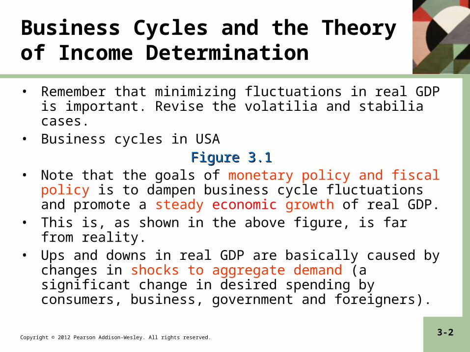
Business Cycles and the Theory of Income Determination
• Remember that minimizing fluctuations in real GDP is important. Revise the volatilia and stabilia cases.
• Business cycles in USA Figure 3.1Figure 3.1
• Note that the goals of monetary policy and fiscal policy is to dampen business cycle fluctuations and promote a steady economic growth of real GDP.
• This is, as shown in the above figure, is far from reality.• Ups and downs in real GDP are basically caused by changes in
shocks to aggregate demand (a significant change in desired spending by consumers, business, government and foreigners).
Copyright © 2012 Pearson Addison-Wesley. All rights reserved. 3-3
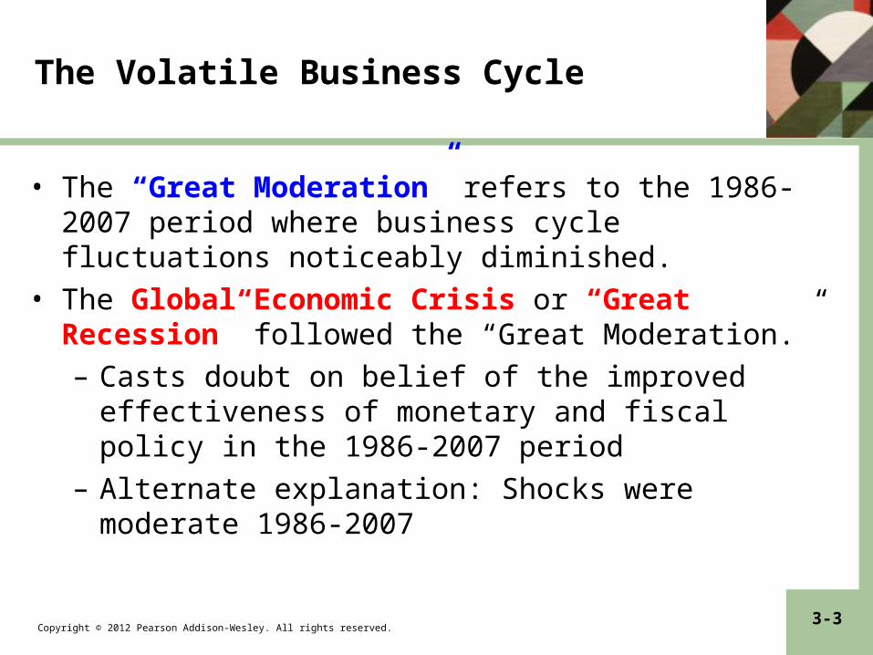
The Volatile Business Cycle
• The “Great Moderation” refers to the 1986-2007 period where business cycle fluctuations noticeably diminished.
• The Global Economic Crisis or “Great Recession” followed the “Great Moderation.”
– Casts doubt on belief of the improved effectiveness of monetary and fiscal policy in the 1986-2007 period
– Alternate explanation: Shocks were moderate 1986-2007
Copyright © 2012 Pearson Addison-Wesley. All rights reserved. 3-4
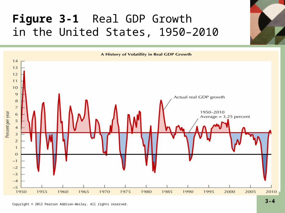
Figure 3-1 Real GDP Growth in the United States, 1950–2010
Copyright © 2012 Pearson Addison-Wesley. All rights reserved. 3-5
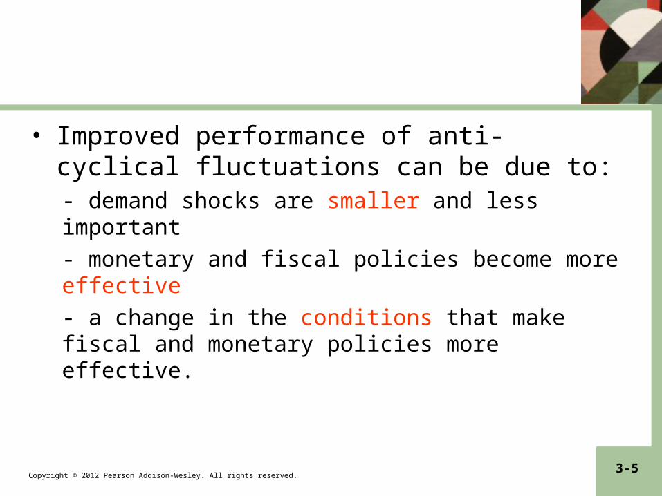
• Improved performance of anti-cyclical fluctuations can be due to:- demand shocks are smaller and less important
- monetary and fiscal policies become more effective
- a change in the conditions that make fiscal and monetary policies more effective.
Copyright © 2012 Pearson Addison-Wesley. All rights reserved. 3-6
The Volatile Business Cycle
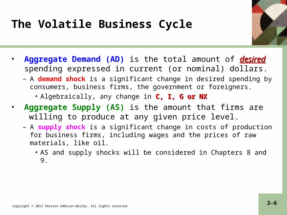
• Aggregate Demand (AD) is the total amount of desireddesired spending expressed in current (or nominal) dollars.– A demand shock is a significant change in desired spending by
consumers, business firms, the government or foreigners.
• Algebraically, any change in C, I, G or NXC, I, G or NX
• Aggregate Supply (AS) is the amount that firms are willing to produce at any given price level.– A supply shock is a significant change in costs of production for business
firms, including wages and the prices of raw materials, like oil.
• AS and supply shocks will be considered in Chapters 8 and 9.

Copyright © 2012 Pearson Addison-Wesley. All rights reserved. 3-7
Income determination and the price level
• Simplifying assumption:– The price level (P) is fixed in the short run.
• Implication: All changes in AD automatically cause changes in real GDP by the same amount and in the same direction.
Change in y = change in AD/p(fixed price)Change in y = change in AD/p(fixed price)
• Is there any evidence to support the assumption that prices are fixed in the short run?
1. Price labels are printed and expensive to reprint
2. Prices of mail order catalogues are set for the entire season
3. Wages and salaries usually change every year and perhaps in more than that.
• Therefore, changes in AD are directly translated into changes in real GDP.
Copyright © 2012 Pearson Addison-Wesley. All rights reserved. 3-8
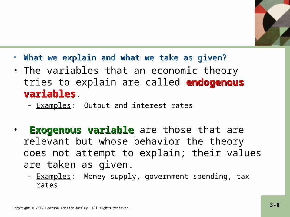
• What we explain and what we take as given?What we explain and what we take as given?
• The variables that an economic theory tries to explain are called endogenous variablesendogenous variables.– Examples: Output and interest rates
• Exogenous variableExogenous variable are those that are relevant but whose behavior the theory does not attempt to explain; their values are taken as given.– Examples: Money supply, government spending, tax rates

Copyright © 2012 Pearson Addison-Wesley. All rights reserved. 3-9
Consumption and Savings
• The consumption function is any relationship that describes the determinants of consumption spending.
• General linear form: C = Cα + c(Y – T) where…
• Cα = Autonomous consumption
• c = marginal propensity to consume
• c(Y – T) = induced consumptionC = 500 + .75 (Y-T)C = 500 + .75 (Y-T)
Copyright © 2012 Pearson Addison-Wesley. All rights reserved. 3-10
Consumption and Savings
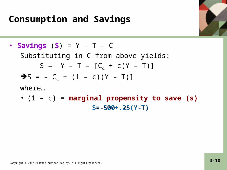
• Savings (S) = Y – T – C
Substituting in C from above yields:
S = Y – T – [Cα + c(Y – T)]
S = – Cα + (1 – c)(Y – T)]
where…
• (1 – c) = marginal propensity to save (s)S=-500+.25(Y-T)S=-500+.25(Y-T)
Copyright © 2012 Pearson Addison-Wesley. All rights reserved. 3-11
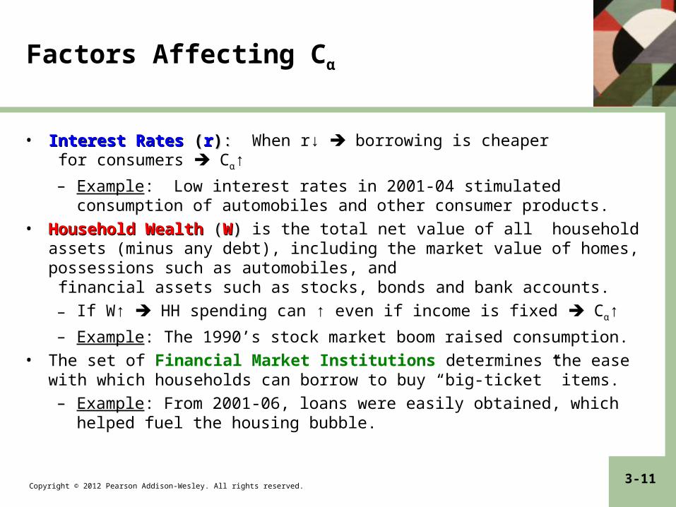
Factors Affecting Cα
• Interest RatesInterest Rates ( (rr)): : When r↓ borrowing is cheaper for consumers Cα↑
– Example: Low interest rates in 2001-04 stimulated consumption of automobiles and other consumer products.
• Household WealthHousehold Wealth ( (WW) ) is the total net value of all household assets (minus any debt), including the market value of homes, possessions such as automobiles, and financial assets such as stocks, bonds and bank accounts.
– If W↑ HH spending can ↑ even if income is fixed Cα↑
– Example: The 1990’s stock market boom raised consumption.
• The set of Financial Market Institutions determines the ease with which households can borrow to buy “big-ticket” items.
– Example: From 2001-06, loans were easily obtained, which helped fuel the housing bubble.
Copyright © 2012 Pearson Addison-Wesley. All rights reserved. 3-12
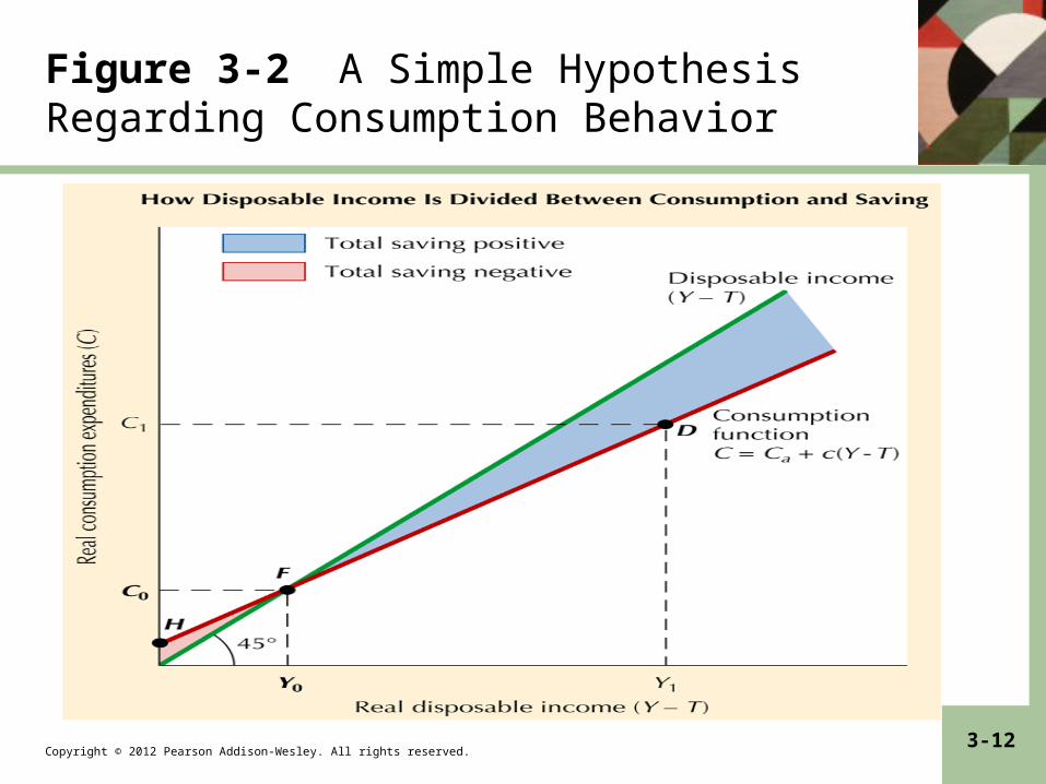
Figure 3-2 A Simple Hypothesis Regarding Consumption Behavior

Copyright © 2012 Pearson Addison-Wesley. All rights reserved. 3-13
Copyright © 2012 Pearson Addison-Wesley. All rights reserved. 3-14
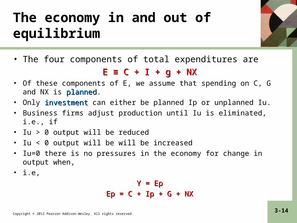
The economy in and out of equilibrium
• The four components of total expenditures are
E ≡ C + I + g + NXE ≡ C + I + g + NX• Of these components of E, we assume that spending on C, G and NX is
plannedplanned.
• Only investmentinvestment can either be planned Ip or unplanned Iu.
• Business firms adjust production until Iu is eliminated, i.e., if
• Iu > 0 output will be reduced
• Iu < 0 output will be will be increased
• Iu=0 there is no pressures in the economy for change in output when,
• i.e,
Y = EpY = Ep
Ep = C + Ip + G + NXEp = C + Ip + G + NX

Copyright © 2012 Pearson Addison-Wesley. All rights reserved. 3-15
• Planned expenditures equals
Ep = Ca + c(Y-T) + Ip + G + NXEp = Ca + c(Y-T) + Ip + G + NX• Note that consumption is composed of autonomous and induced.
• Autonomous planned spending
• Autonomous planned spending (Ap) is the spending that does not depend on total income (Y); i.e.,
AApp = E – cY = C = E – cY = Caa – cT – cTaa + I + Ipp + G + NX + G + NX
(cY induced consumption)• -cTa is the effect of autonomous taxes in reducing C (note that we
assume that taxes as autonomous).
Copyright © 2012 Pearson Addison-Wesley. All rights reserved. 3-16
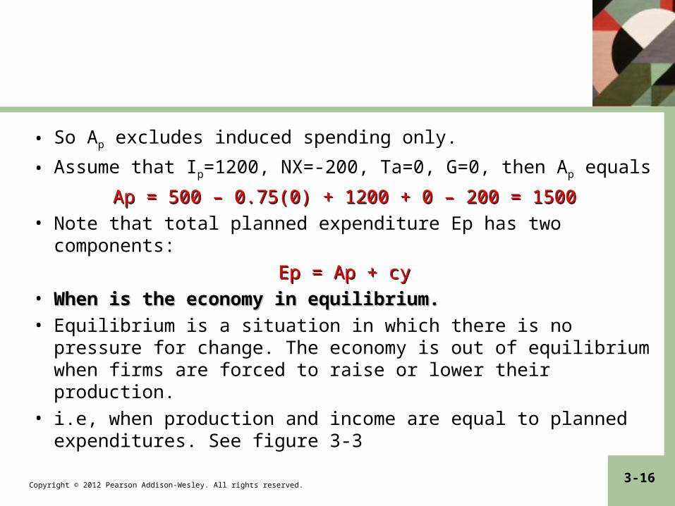
• So Ap excludes induced spending only.
• Assume that Ip=1200, NX=-200, Ta=0, G=0, then Ap equals
Ap = 500 – 0.75(0) + 1200 + 0 – 200 = 1500Ap = 500 – 0.75(0) + 1200 + 0 – 200 = 1500
• Note that total planned expenditure Ep has two components:
Ep = Ap + cyEp = Ap + cy
• When is the economy in equilibrium. When is the economy in equilibrium.
• Equilibrium is a situation in which there is no pressure for change. The economy is out of equilibrium when firms are forced to raise or lower their production.
• i.e, when production and income are equal to planned expenditures. See figure 3-3
Copyright © 2012 Pearson Addison-Wesley. All rights reserved. 3-17
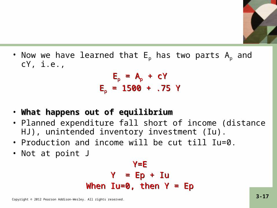
• Now we have learned that Ep has two parts Ap and cY, i.e.,
EEpp = A = App + cY + cY
EEpp = 1500 + .75 Y = 1500 + .75 Y
• What happens out of equilibriumWhat happens out of equilibrium• Planned expenditure fall short of income (distance HJ),
unintended inventory investment (Iu). • Production and income will be cut till Iu=0. • Not at point J
Y=EY=EY = Ep + IuY = Ep + Iu
When Iu=0, then Y = EpWhen Iu=0, then Y = Ep

Copyright © 2012 Pearson Addison-Wesley. All rights reserved. 3-18
Figure 3-3 the Keynesian Cross Model of Income Determination.

Copyright © 2012 Pearson Addison-Wesley. All rights reserved. 3-19
Figure 3-3 the Keynesian Cross Model of Income Determination.

Copyright © 2012 Pearson Addison-Wesley. All rights reserved. 3-20
Table 3-1 Comparison of the Economy’s “Always True” and Equilibrium Situations
Copyright © 2012 Pearson Addison-Wesley. All rights reserved. 3-21
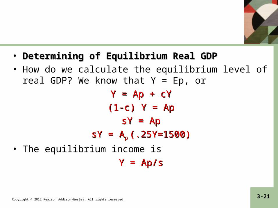
• Determining of Equilibrium Real GDPDetermining of Equilibrium Real GDP
• How do we calculate the equilibrium level of real GDP? We know that Y = Ep, or
Y = Ap + cYY = Ap + cY
(1-c) Y = Ap(1-c) Y = Ap
sY = ApsY = Ap
sY = AsY = App (.25Y=1500)(.25Y=1500)
• The equilibrium income is
Y = Ap/sY = Ap/s

Copyright © 2012 Pearson Addison-Wesley. All rights reserved. 3-22
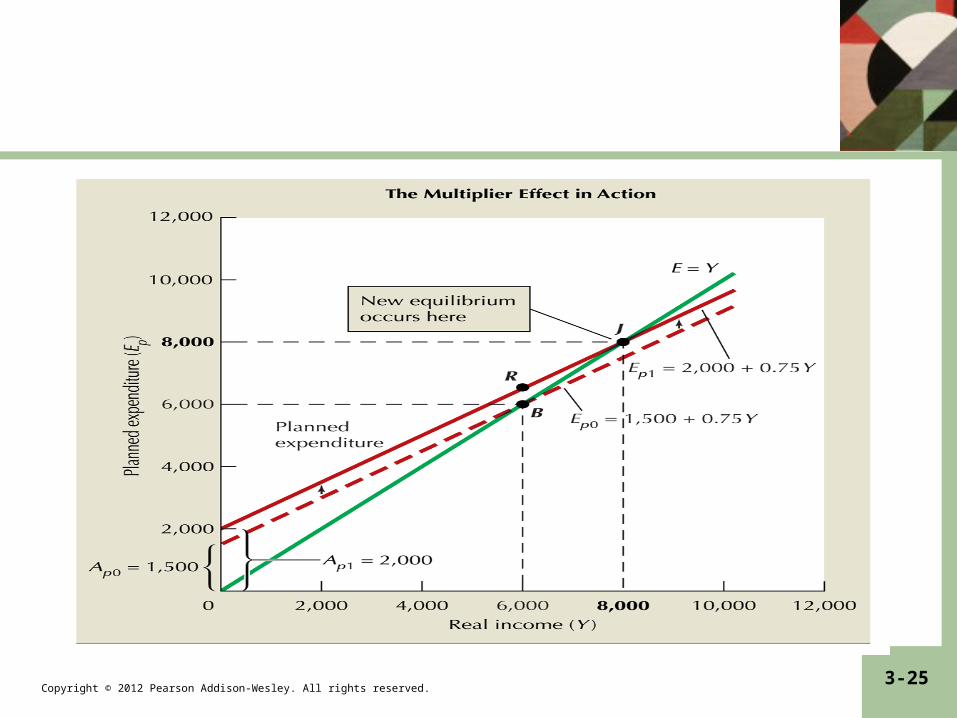
The Multiplier Effect
• Any change in Ap will cause a change in equilibrium income.
• Suppose that businesses raise their investment by 500, i.e., Ap increases from 1500 (Ap0) to 2000 (Ap1). The effect of a change in Ap can be illustrated.
• Calculating the Multiplier Calculating the Multiplier
• To calculate the equilibrium level of income in the new and old situations. Note – New equilibrium New equilibrium Y1 = AY1 = Ap1p1/s = 2000/.25 = 8000/s = 2000/.25 = 8000– Subtract from old Subtract from old Y0 = AY0 = Ap0p0/s = 1500/.25 = 6000/s = 1500/.25 = 6000– Equals change in income Equals change in income ∆Y = ∆A∆Y = ∆App/s = 500/.25 = 2000/s = 500/.25 = 2000
Copyright © 2012 Pearson Addison-Wesley. All rights reserved. 3-23
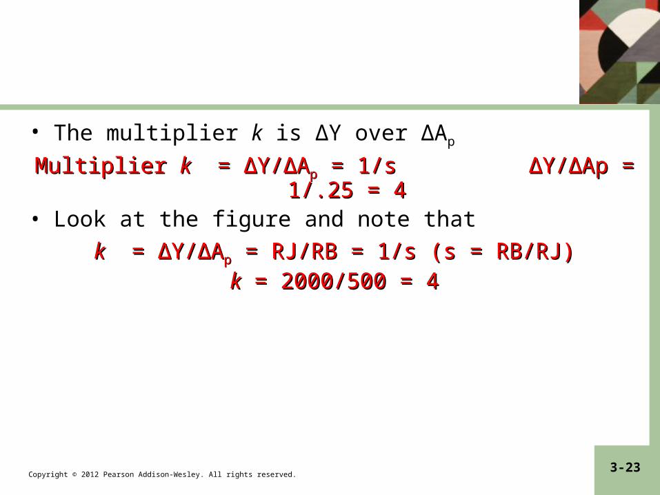
• The multiplier k is ∆Y over ∆Ap
Multiplier Multiplier kk = ∆Y/∆A = ∆Y/∆App = 1/s ∆Y/∆Ap = 1/.25 = 4 = 1/s ∆Y/∆Ap = 1/.25 = 4• Look at the figure and note that
kk = ∆Y/∆A = ∆Y/∆App = RJ/RB = 1/s (s = RB/RJ) = RJ/RB = 1/s (s = RB/RJ)
kk = 2000/500 = 4 = 2000/500 = 4

Copyright © 2012 Pearson Addison-Wesley. All rights reserved. 3-24
Figure 3-4 The Change in Equilibrium Income Caused by a $500 Billion Increase in Autonomous Planned Spending
Copyright © 2012 Pearson Addison-Wesley. All rights reserved. 3-25
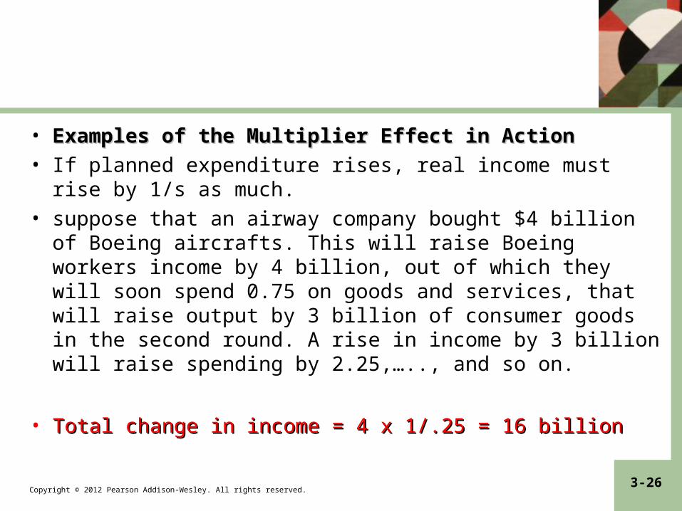
Copyright © 2012 Pearson Addison-Wesley. All rights reserved. 3-26
• Examples of the Multiplier Effect in ActionExamples of the Multiplier Effect in Action
• If planned expenditure rises, real income must rise by 1/s as much.
• suppose that an airway company bought $4 billion of Boeing aircrafts. This will raise Boeing workers income by 4 billion, out of which they will soon spend 0.75 on goods and services, that will raise output by 3 billion of consumer goods in the second round. A rise in income by 3 billion will raise spending by 2.25,….., and so on.
• Total change in income = 4 x 1/.25 = 16 billion Total change in income = 4 x 1/.25 = 16 billion
Copyright © 2012 Pearson Addison-Wesley. All rights reserved. 3-27
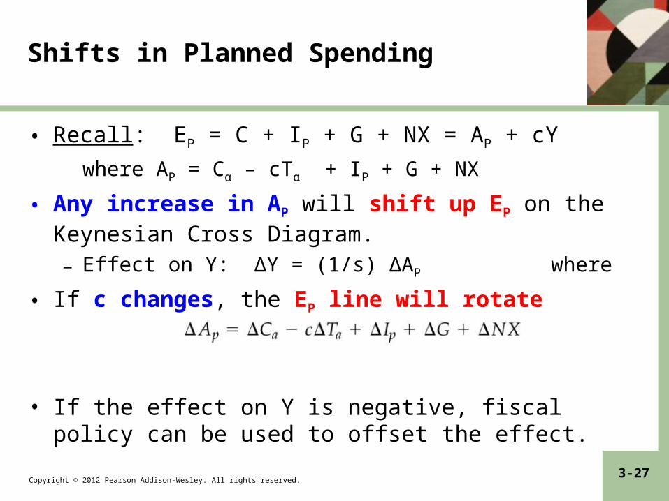
Shifts in Planned Spending
• Recall: EP = C + IP + G + NX = AP + cY
where AP = Cα – cTα + IP + G + NX
• Any increase in AP will shift up EP on the Keynesian Cross Diagram.– Effect on Y: ∆Y = (1/s) ∆AP where
• If c changes, the EP line will rotate
• If the effect on Y is negative, fiscal policy can be used to offset the effect.
Copyright © 2012 Pearson Addison-Wesley. All rights reserved. 3-28
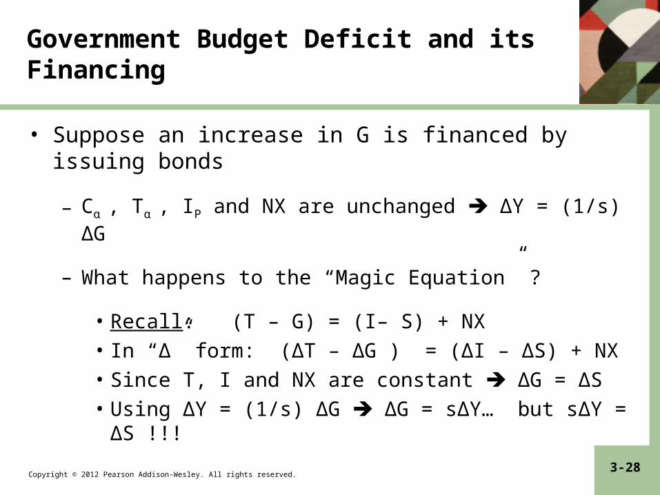
Government Budget Deficit and its Financing
• Suppose an increase in G is financed by issuing bonds
– Cα , Tα , IP and NX are unchanged ∆Y = (1/s) ∆G
– What happens to the “Magic Equation” ?
• Recall: (T – G) = (I– S) + NX
• In “∆” form: (∆T – ∆G ) = (∆I – ∆S) + NX
• Since T, I and NX are constant ∆G = ∆S
• Using ∆Y = (1/s) ∆G ∆G = s∆Y… but s∆Y = ∆S !!!
Copyright © 2012 Pearson Addison-Wesley. All rights reserved. 3-29
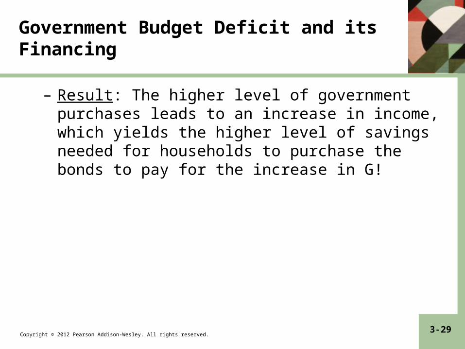
Government Budget Deficit and its Financing
– Result: The higher level of government purchases leads to an increase in income, which yields the higher level of savings needed for households to purchase the bonds to pay for the increase in G!

Copyright © 2012 Pearson Addison-Wesley. All rights reserved. 3-30
Government Budget Deficit and its Financing
– The Tax Multiplier
• The tax multiplier
• As an alternative to using G by 500, the government can reduce taxes by 667 ((2000/0.75)*0.25) to have the same impact. Thus;
∆Y = -(.75)(-667)/.25 = 500/.25 = 2000
• The multiplier is –c/s:
∆Y/∆Ta = -c/s
Copyright © 2012 Pearson Addison-Wesley. All rights reserved. 3-31
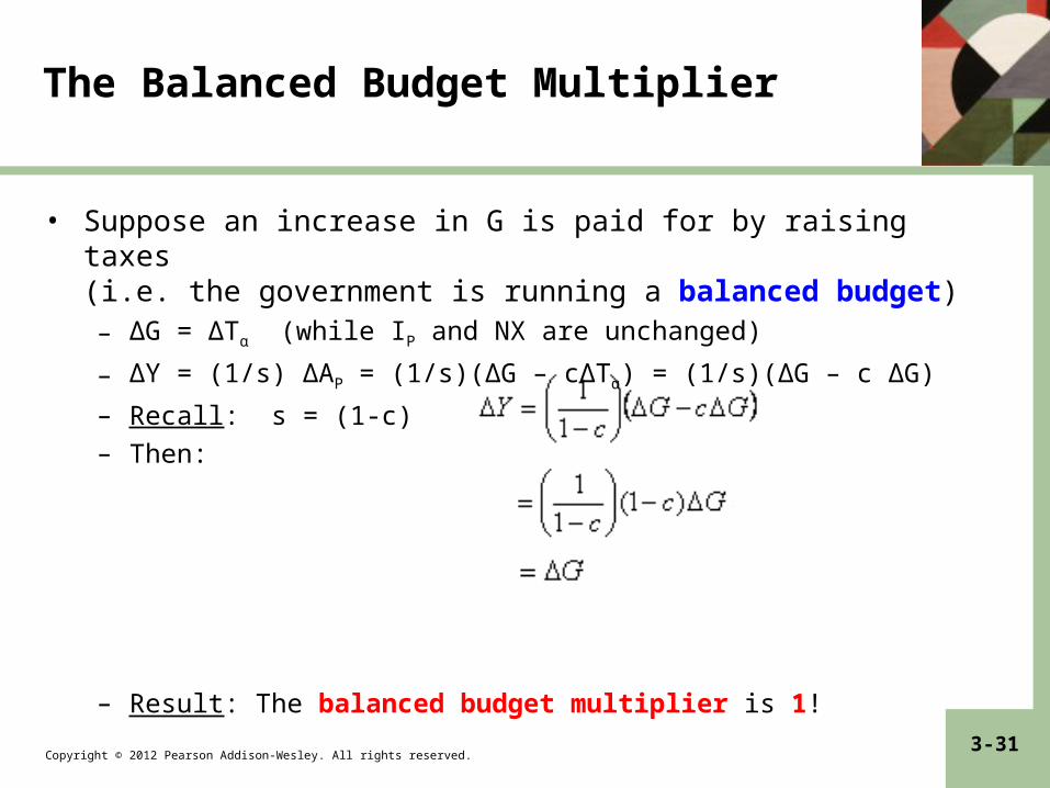
The Balanced Budget Multiplier
• Suppose an increase in G is paid for by raising taxes(i.e. the government is running a balanced budget)– ∆G = ∆Tα (while IP and NX are unchanged)
– ∆Y = (1/s) ∆AP = (1/s)(∆G – c∆Tα) = (1/s)(∆G – c ∆G)
– Recall: s = (1-c)
– Then:
– Result: The balanced budget multiplier is 1!
Copyright © 2012 Pearson Addison-Wesley. All rights reserved. 3-32
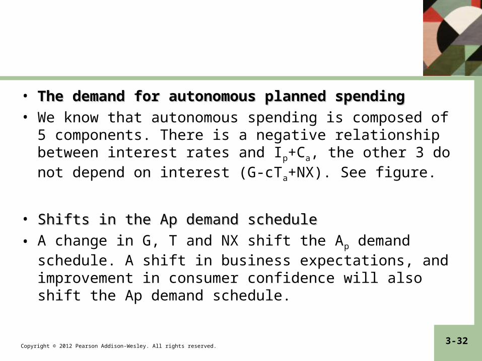
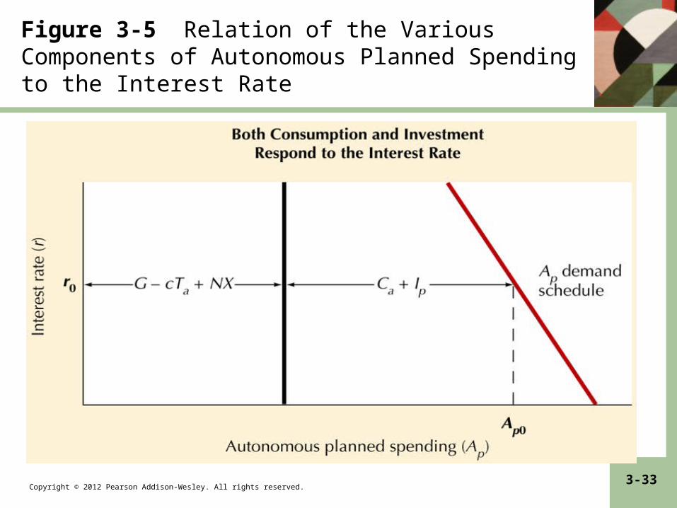
• The demand for autonomous planned spendingThe demand for autonomous planned spending
• We know that autonomous spending is composed of 5 components. There is a negative relationship between interest rates and Ip+Ca, the other 3 do not depend on interest (G-cTa+NX). See figure.
• Shifts in the Ap demand schedule Shifts in the Ap demand schedule
• A change in G, T and NX shift the Ap demand schedule. A shift in business expectations, and improvement in consumer confidence will also shift the Ap demand schedule.
Copyright © 2012 Pearson Addison-Wesley. All rights reserved. 3-33
Figure 3-5 Relation of the Various Components of Autonomous Planned Spending to the Interest Rate
Copyright © 2012 Pearson Addison-Wesley. All rights reserved. 3-34
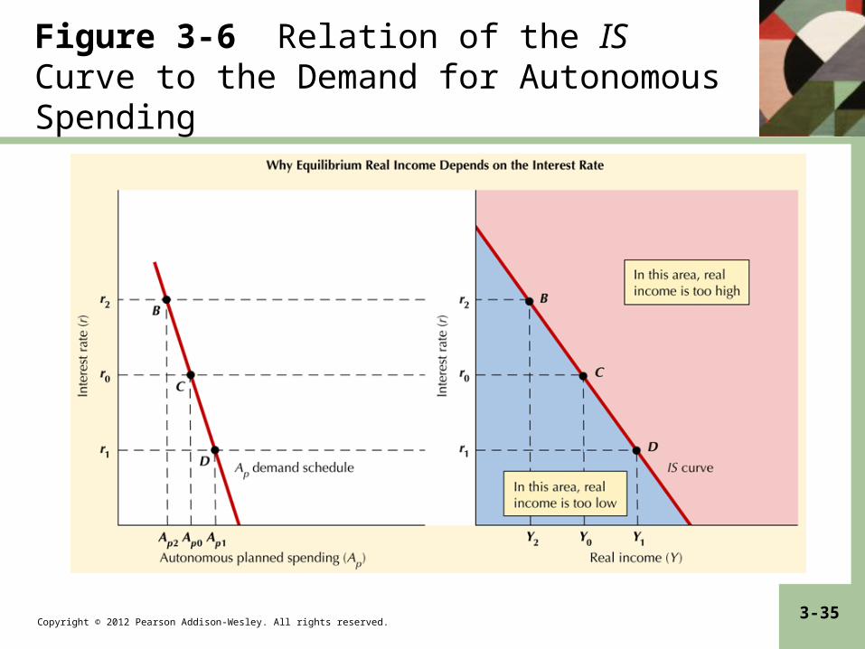
• The IS curve The IS curve
• Ap depends on interest rate. Real GDP and real income depend on Ap, therefore, real GDP and real income depend on interest rate. The IS curve shows the different combinations of interest rate and real income that are compatible with equilibrium.
• How to derive the IS curve. How to derive the IS curve.
• the LHS OF figure 3-9 shows the demand for Ap at different levels of interest rates. Assume that there are no G, T, and NX, so that Ap consists of Ip + Ca, both is negatively related to interest rate. Given a multiplier of 4, at different points of Ap, real income is determined.
Copyright © 2012 Pearson Addison-Wesley. All rights reserved. 3-35
Figure 3-6 Relation of the IS Curve to the Demand for Autonomous Spending
Copyright © 2012 Pearson Addison-Wesley. All rights reserved. 3-36
• What the IS curve showsWhat the IS curve shows
• The IS shows different combinations of interest rate (r) and income (y), at which the market is in equilibrium when y = Ap. At any point out of the IS the economy is out of equilibrium.
Copyright © 2012 Pearson Addison-Wesley. All rights reserved. 3-37
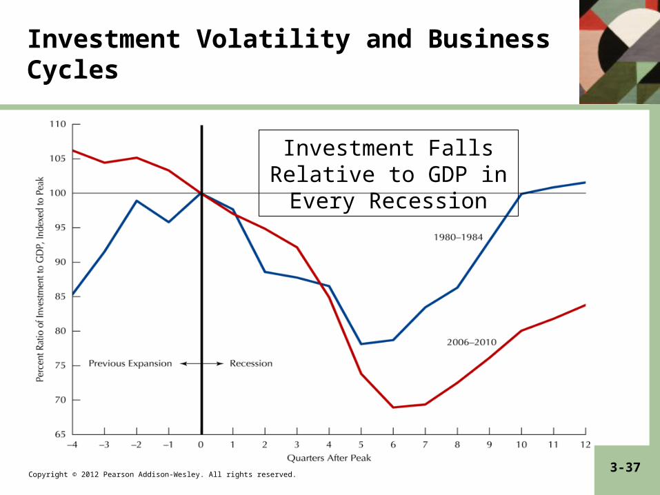
Investment Volatility and Business Cycles
Investment Falls Relative to GDP in Every Recession

Copyright © 2012 Pearson Addison-Wesley. All rights reserved. 3-38