
Copyright 2010, Lin Cong
90
Joint Solution of Urban Structure Detection from Hyperion Hyperspectral Images by Lin Cong, B.S. A THESIS IN ELECTRICAL ENGINEERING Submitted to the Graduate Faculty of Texas Tech University in Partial Fulfillment of the Requirements for the Degree of MASTER OF SCIENCE IN ELECTRICAL ENGINEERING Approved Dr. Brian Nutter Chair of Committee Dr. Daan Liang Dr. Sunanda Mitra Peggy Gordon Miller Dean of the Graduate School December, 2010
Transcript of Copyright 2010, Lin Cong

Joint Solution of Urban Structure Detection from Hyperion Hyperspectral Images
by
Lin Cong, B.S.
A THESIS
IN
ELECTRICAL ENGINEERING
Submitted to the Graduate Faculty of Texas Tech University in
Partial Fulfillment of the Requirements for
the Degree of
MASTER OF SCIENCE IN
ELECTRICAL ENGINEERING
Approved
Dr. Brian Nutter Chair of Committee
Dr. Daan Liang
Dr. Sunanda Mitra
Peggy Gordon Miller Dean of the Graduate School
December, 2010

Copyright 2010, Lin Cong

Texas Tech University, Lin Cong, December 2010
ii
ACKNOWLEDGMENTS I would like to express my sincere gratitude to my advisors Dr. Brian Nutter
and Dr. Daan Liang for giving me an opportunity to work in the field of hyperspectral
satellite imaging. This thesis wouldn’t be possible without their continuous support
during my entire Masters program at Texas Tech University. Dr. Nutter was always
available to guide me to the correct method for digital signal/image processing, and
Dr. Liang provided me with the necessary hurricane damage information and study
tools. I sincerely thank them for patiently revising my thesis and other publications
and providing many valuable suggestions. Also, I want to thank my committee
member Dr. Sunanda Mitra for coming to my defense and providing valuable
suggestions.
I would also like to thank my fellow students Enrique Corona, Dr. Zheng Liu
and Jingqi Ao. Enrique provided me with Jump code for model order estimation and
Dr. Liu also helped me in the image processing. Those guys are valuable resources in
the lab whenever I have problems.
Last but not least, I would like to thank my parents back in China and all my
friends for their support and encouragement.
Texas Tech University, Lin Cong, December 2010
iii
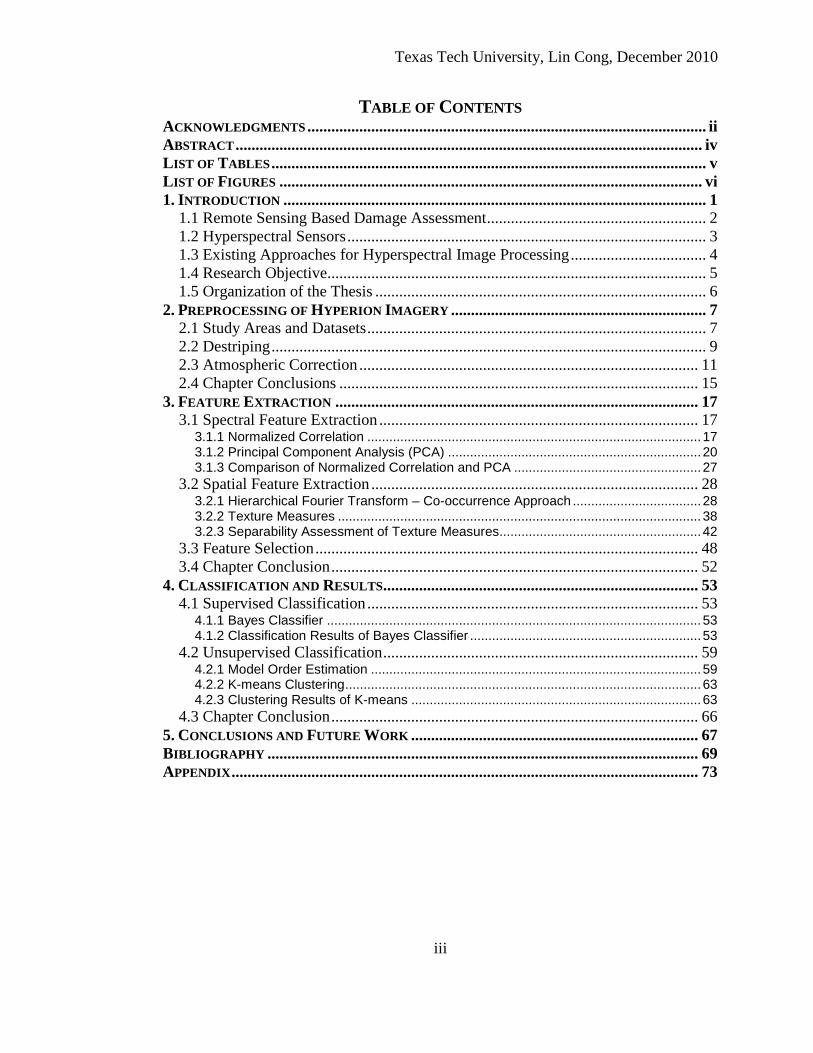
TABLE OF CONTENTS ACKNOWLEDGMENTS .................................................................................................... ii ABSTRACT ..................................................................................................................... iv LIST OF TABLES ............................................................................................................. v LIST OF FIGURES .......................................................................................................... vi 1. INTRODUCTION .......................................................................................................... 1
1.1 Remote Sensing Based Damage Assessment ....................................................... 2 1.2 Hyperspectral Sensors .......................................................................................... 3 1.3 Existing Approaches for Hyperspectral Image Processing .................................. 4 1.4 Research Objective............................................................................................... 5 1.5 Organization of the Thesis ................................................................................... 6
2. PREPROCESSING OF HYPERION IMAGERY ................................................................ 7 2.1 Study Areas and Datasets ..................................................................................... 7 2.2 Destriping ............................................................................................................. 9 2.3 Atmospheric Correction ..................................................................................... 11 2.4 Chapter Conclusions .......................................................................................... 15
3. FEATURE EXTRACTION ........................................................................................... 17 3.1 Spectral Feature Extraction ................................................................................ 17
3.1.1 Normalized Correlation ........................................................................................... 17 3.1.2 Principal Component Analysis (PCA) ..................................................................... 20 3.1.3 Comparison of Normalized Correlation and PCA ................................................... 27
3.2 Spatial Feature Extraction .................................................................................. 28 3.2.1 Hierarchical Fourier Transform – Co-occurrence Approach ................................... 28 3.2.2 Texture Measures ................................................................................................... 38 3.2.3 Separability Assessment of Texture Measures....................................................... 42
3.3 Feature Selection ................................................................................................ 48 3.4 Chapter Conclusion ............................................................................................ 52
4. CLASSIFICATION AND RESULTS ............................................................................... 53 4.1 Supervised Classification ................................................................................... 53
4.1.1 Bayes Classifier ...................................................................................................... 53 4.1.2 Classification Results of Bayes Classifier ............................................................... 53
4.2 Unsupervised Classification ............................................................................... 59 4.2.1 Model Order Estimation .......................................................................................... 59 4.2.2 K-means Clustering ................................................................................................. 63 4.2.3 Clustering Results of K-means ............................................................................... 63
4.3 Chapter Conclusion ............................................................................................ 66 5. CONCLUSIONS AND FUTURE WORK ........................................................................ 67 BIBLIOGRAPHY ............................................................................................................ 69 APPENDIX ..................................................................................................................... 73
Texas Tech University, Lin Cong, December 2010
iv
ABSTRACT Hyperspectral remote sensing has shown great potential for disaster analysis.
In post-disaster urban damage assessment, residential areas and buildings must be
accurately identified in the images before and after the disaster. However, the
traditional spectral-only or spatial-only solutions prove ineffective for residence
detection from low resolution hyperspectral images, such as Hyperion data. To solve
this problem, a joint solution of residential area classification, based on both spectral
signature and spatial texture, is proposed in this thesis. Correlations between every
pixel spectrum and the selected endmembers’ spectra and the most significant PCA
(Principle Component Analysis) components of the spectral data provide spectral
features of every pixel. A hierarchical Fourier Transform – Co-occurrence Matrix
approach is designed to help capture spatial textures. Eight second order texture
measures are calculated based on the co-occurrence matrix, and K-fold cross
validation is performed on the training data to select the best combination of features
for the proposed algorithm.
Compared with most existing methods that focus exclusively on spectral or
spatial information and rely on high spatial resolution hyperspectral images that are
usually taken by airborne sensors, our solution makes use of both spectral signature
and macroscopic grid patterns of the residential areas and hence works well for low
resolution Hyperion imagery.
Texas Tech University, Lin Cong, December 2010
v
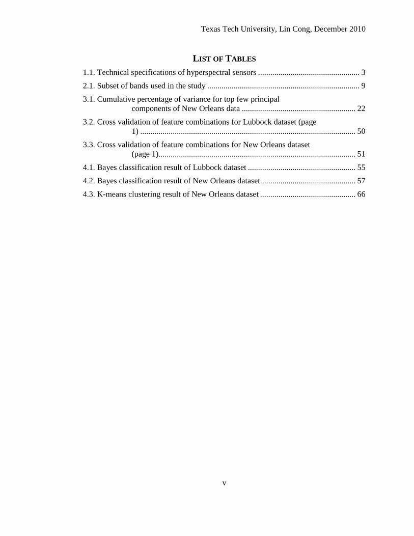
LIST OF TABLES 1.1. Technical specifications of hyperspectral sensors .................................................. 3
2.1. Subset of bands used in the study ........................................................................... 9
3.1. Cumulative percentage of variance for top few principal components of New Orleans data ........................................................ 22
3.2. Cross validation of feature combinations for Lubbock dataset (page 1) .......................................................................................................... 50
3.3. Cross validation of feature combinations for New Orleans dataset (page 1)................................................................................................. 51
4.1. Bayes classification result of Lubbock dataset ..................................................... 55
4.2. Bayes classification result of New Orleans dataset............................................... 57
4.3. K-means clustering result of New Orleans dataset ............................................... 66
Texas Tech University, Lin Cong, December 2010
vi
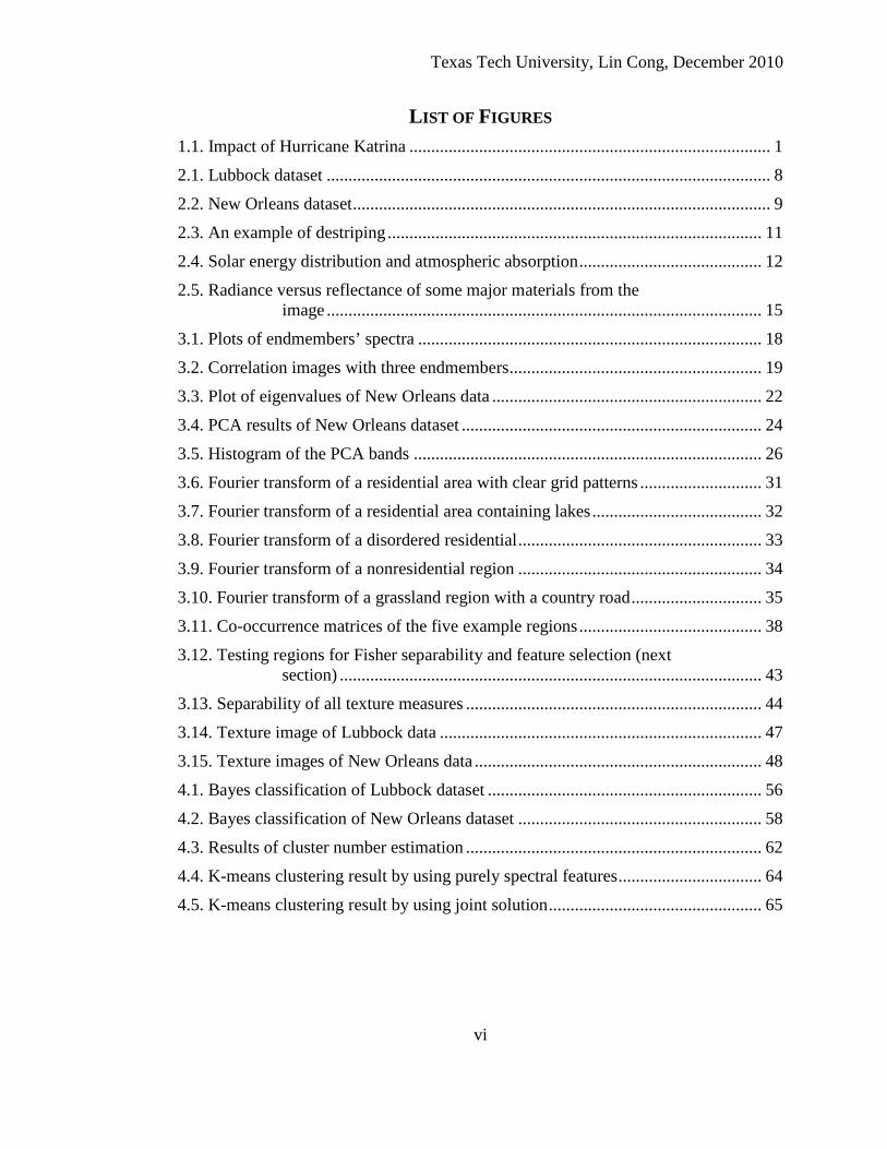
LIST OF FIGURES 1.1. Impact of Hurricane Katrina ................................................................................... 1
2.1. Lubbock dataset ...................................................................................................... 8
2.2. New Orleans dataset ................................................................................................ 9
2.3. An example of destriping ...................................................................................... 11
2.4. Solar energy distribution and atmospheric absorption .......................................... 12
2.5. Radiance versus reflectance of some major materials from the image .................................................................................................... 15
3.1. Plots of endmembers’ spectra ............................................................................... 18
3.2. Correlation images with three endmembers .......................................................... 19
3.3. Plot of eigenvalues of New Orleans data .............................................................. 22
3.4. PCA results of New Orleans dataset ..................................................................... 24
3.5. Histogram of the PCA bands ................................................................................ 26
3.6. Fourier transform of a residential area with clear grid patterns ............................ 31
3.7. Fourier transform of a residential area containing lakes ....................................... 32
3.8. Fourier transform of a disordered residential ........................................................ 33
3.9. Fourier transform of a nonresidential region ........................................................ 34
3.10. Fourier transform of a grassland region with a country road .............................. 35
3.11. Co-occurrence matrices of the five example regions .......................................... 38
3.12. Testing regions for Fisher separability and feature selection (next section) ................................................................................................. 43
3.13. Separability of all texture measures .................................................................... 44
3.14. Texture image of Lubbock data .......................................................................... 47
3.15. Texture images of New Orleans data .................................................................. 48
4.1. Bayes classification of Lubbock dataset ............................................................... 56
4.2. Bayes classification of New Orleans dataset ........................................................ 58
4.3. Results of cluster number estimation .................................................................... 62
4.4. K-means clustering result by using purely spectral features ................................. 64
4.5. K-means clustering result by using joint solution ................................................. 65

Texas Tech University, Lin Cong, December 2010
1
CHAPTER I
INTRODUCTION Hurricanes cause an extraordinary level of property losses and human
suffering, with an estimated annualized cost of $6.3 billion in the United States [1].
Recent experiences with Hurricane Katrina and Rita of 2005 once again underscore
this nation’s increasing vulnerability to hurricane disasters in spite of significant
progress made in weather forecasting and hazard preparation. According to [2], 1577
people were killed in the state of Louisiana, and almost 900,000 people in the state lost
power as a result of the Hurricane Katrina. More and more attention has been paid to
the implementation of advanced technologies to produce information that will help
reduce future hurricane losses. Remote sensing technology can be the keystone of an
integrated support system for disaster response, recovery and mitigation.
(a) (b)
Figure 1.1. Impact of Hurricane Katrina (a): Flooded I-10/I-610/West End Blvd interchange and surrounding area of northwest New Orleans and Metairie, Louisiana [3]; (b): Damage to Long Beach, Mississippi, following Hurricane Katrina [4].
Texas Tech University, Lin Cong, December 2010
2
1.1 Remote Sensing Based Damage Assessment Remote sensing and Geographical Information System (GIS) data have
become an increasingly important resource for the disaster management community.
Although hurricane disasters are inevitable, it is possible to minimize the potential risk
by developing disaster early warning strategies, to prepare and implement
developmental plans that provide resilience to such disasters, and to help in
rehabilitation and post-disaster reduction [5]. Remote sensing and GIS play a major
role in efficient mitigation and management of hazards.
A variety of satellites carrying different sensors have been launched in past
decades. Although none of the sensors has been designed solely for the purpose of
observing natural disasters, the variety of spectral bands in VIS (visible), NIR (near
infrared), SWIR (short wave infrared), TIR (thermal infrared) and SAR (synthetic
aperture radar) covers adequate electromagnetic spectrum and provides different
information about properties of the surface. For instance, measurements of the
reflected solar radiation give information on albedo (fraction of light that is reflected
by a body or surface), thermal sensors measure surface temperature, and microwave
sensors measure the dielectric properties, and hence the moisture content, of surface
soil or snow [6]. Compared with VIS, thermal and SAR sensors, multispectral sensors
that usually have 5 to 10 spectral bands from VIS to SWIR (or even TIR) are more
widely used for general disaster management, including hurricane assessment.
The crude spectral categorization of the reflected and emitted energy from the
earth is a limiting factor of multispectral sensor systems [7]. Over the past decades,
advances in sensor technology have overcome this limitation with the development of
hyperspectral sensor technologies. Hyperspectral sensors collect spectral information
as a set of “images”. Each image represents a narrow range of the electromagnetic
spectrum known as a spectral band. These images are combined to form a three
dimensional hyperspectral cube for the surface of the Earth. One significant feature
separating a hyperspectral imager from other optical sensors such as a multispectral
imager is that a hyperspectral spectrometer measures radiation in a series of narrow
and contiguous wavelength bands, usually from the ultraviolet to infrared. A

Texas Tech University, Lin Cong, December 2010
3
multispectral spectrometer, on the other hand, measures radiation at a few widely
separated wavelength bands [8]. Due to the sufficiency of spectral information,
hyperspectral imagery provides an opportunity for more comprehensive and detailed
representation of surface material.
1.2 Hyperspectral Sensors A number of private companies, academic institutions, and government
agencies have capabilities to acquire hyperspectral imagery, including the European
Space Agency (ESA) and the National Aeronautics and Space Administration
(NASA). Table 1.1 lists some of the currently active hyperspectral imagers along with
their technical specifications. Based on the EO – 1 satellite, Hyperion has a preferable
availability immediately after a hurricane and it is completely free to public access.
With the consideration of availability and access, this study focuses on images from
the Hyperion sensor.
Table 1.1. Technical specifications of hyperspectral sensors Sensor Operator Spectral
Resolution
Spatial
Resolution
Swath
Width
Platform
AVIRIS NASA/JPL 224 bands (400
– 2500 nm)
20 m (h. alt.)
4 m (l. alt.)
11 km
1.9 km
ER – 2
aircraft
Hyperion NASA/USGS 242 bands (356
– 2577 nm)
30 m 7.7 km EO – 1
CHRIS ESA 200 bands (415
– 1050 nm)
20 m 14 km Proba
HyMap Integrated
Spectronics
(Australia)
128 bands (450
– 2480 nm)
5 m (2km alt.) 2.3 km
(2km alt.)
Cessna
aircraft
CASI ITRES (Canada) 288 bands (380
– 1050 nm)
1.5 m 2.25 km aircraft
HYDICE Hughes Danbury
Optical Systems
210 bands (400
– 2500 nm)
1 – 4 m 270 m
(lowest.)
CV – 580
aircraft

Texas Tech University, Lin Cong, December 2010
4
1.3 Existing Approaches for Hyperspectral Image Processing Many new image processing techniques have been developed for hyperspectral
imagery since the 1990s, most of which can be categorized into one of the two general
categories, pixel level classification and sub-pixel level classification. Among pixel
level methods, Spectral Angle Mapper (SAM) computes a spectral angle between each
pixel spectrum and each endmember spectrum [9] [10]. Endmembers represent
spectral signatures considered macroscopically pure. The smaller the spectral angle,
the more similar the pixel and the endmember are. One of many advantages of SAM is
that it is not sensitive to illumination conditions, because only the directions of
spectral vectors are considered, not the magnitude. Another widely used pixel level
classification method is by matching absorption features at specific positions in the
spectra [11] - [14]. This method is implemented in the ENVI© software application as
Spectral Feature Fitting [15].
Among several sub-pixel classification approaches, the “Spectral Hourglass”
was assessed first to extract endmembers from hyperspectral images and then to use
endmembers to linearly unmix every pixel [16]. This method was successfully applied
to detect minerals at mining sites. However, finding all the endmembers for complex
environments, such as urban areas, is difficult, because most land cover objects in
urban regions are smaller than the spatial resolution of many hyperspectral sensors.
Also, the very large number of endmembers in an urban region usually makes linear
spectral unmixing difficult to implement. In order to simplify heterogeneous urban
surfaces, Ridd proposed the Vegetation – Impervious surface – Soil (VIS) model, by
which every pixel in an urban environment can be explained through proportions of
vegetation, impervious surface and soil [17-18]. As a combination and extension of
both [16] and [17], [19] and [20] developed the Multiple Endmember Spectral Mixture
Analysis (MESMA) technique, which models spectra as a linear sum of spectrally
pure endmembers that vary on a per-pixel basis, rather than using the same set of
endmembers to unmix every pixel. Thus, the full set of endmembers is divided into
three subsets, i.e. vegetation, impervious surface and soil, and every model used to
unmix pixels contains three endmembers, one from each subset.

Texas Tech University, Lin Cong, December 2010
5
Generally, the spectral analysis methods listed above achieved great success in
geology applications but were not as successful in urban remote sensing. It was
reported that even the sophisticated MESMA technique had signature confusion
problems between dry exposed soil and bright impervious surface [21] and that a
spatial resolution of at least 5 m is required in order to adequately capture urban
structures [20] [22].
In addition to spectral processing, spatial analysis is also widely used in remote
sensing. Algorithms based on Fourier transform [23], wavelet transform [24] - [26],
co-occurrence matrices [27] - [29], Gauss-Markov models [30] etc. have been
developed to capture the land cover textures. Microscopic textures have been
successfully utilized in agricultural classification, iceberg detection and urban
structure detection with (very) high resolution remote sensors (usually not
hyperspectral imagers). However, less work has been done for macroscopic urban
textures in low resolution data.
1.4 Research Objective One of the key premises for post-disaster remote sensing-based damage
assessment is the separation of built environment from the natural environment.
However, the traditional spectral-only or spatial-only approaches prove ineffective for
residence detection from low resolution hyperspectral images. Therefore, a joint
solution of residential area classification, based on both spectral signature and spatial
texture, is proposed in this thesis. Correlations between every pixel spectrum and the
selected endmembers’ spectra and the most significant PCA (Principle Component
Analysis) components of the spectral data provide spectral features of every pixel. A
hierarchical Fourier Transform – Co-occurrence Matrix approach is designed to help
capture spatial textures. Eight second order texture measures are calculated based on
the co-occurrence matrix, and K-fold cross validation is performed on the training data
to select the best combination of features for the proposed algorithm.
Compared with existing methods that rely on hyperspectral images in high
spatial resolution, the proposed joint solution makes use of both spectral signature and

Texas Tech University, Lin Cong, December 2010
6
macroscopic grid patterns of the residential areas and works well for low resolution
Hyperion imagery.
1.5 Organization of the Thesis In this chapter, the background of remote sensing-based disaster assessment
and many spectral and spatial analysis techniques of hyperspectral image processing
are reviewed. The objectives of this thesis are also explained. In Chapter II, the data
used in the research is first introduced. Preprocessing to remove the vertical stripe
noise from sensor errors and convert the radiance captured by sensors to the surface
reflectance is then explained. The spectral and spatial feature extractions for the joint
solution are explained in Chapter III. In Chapter IV, the results of both supervised and
unsupervised classification are presented and discussed. Conclusions are made, and
possible future work is previewed in Chapter V.

Texas Tech University, Lin Cong, December 2010
7
CHAPTER II
PREPROCESSING OF HYPERION IMAGERY In this chapter, the image quality of the original Hyperion data is enhanced by
performing histogram normalization for each band. Also, the on-sensor radiance is
converted to surface reflectance by the Fast Line-of-sight Atmospheric Analysis of
Spectral Hypercubes (FLAASH) module in the ENVI© software application.
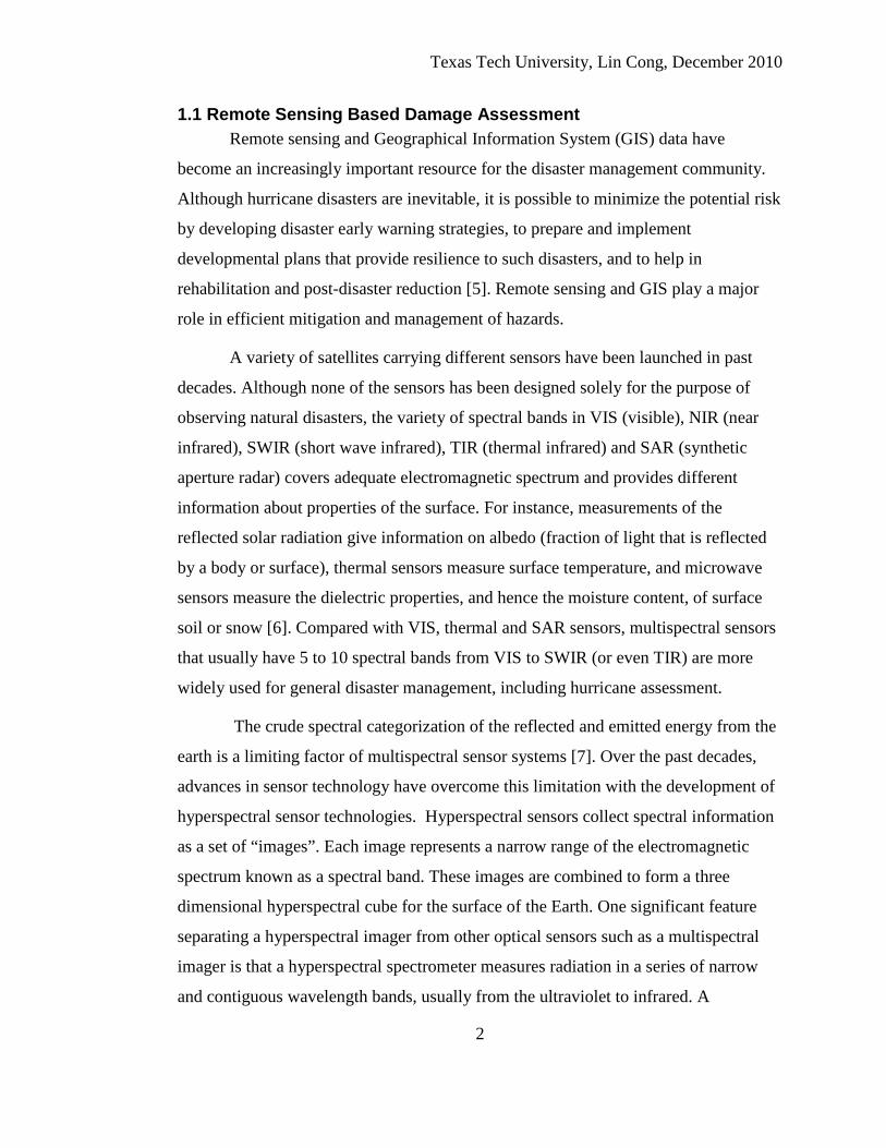
2.1 Study Areas and Datasets This work selected two study areas. The first area is within the City of
Lubbock, TX, centered around 33°34.5’N, 101°53’W, with a population about
210,000. One important and relevant attribute of Lubbock is that most roads in the city
are built from asphalt or concrete, with only a few exceptions built from bricks. An
EO1 Hyperion scene acquired on January 5th, 2003, was used. A 150 km2 region
centered on Lubbock was subset from Hyperion L1R data (not georegistered format)
as shown in Fig. 2.1a. The second study area is within the City of New Orleans, LA,
centered around 29°58.5’N, 90°12.7’W. An EO1 Hyperion scene was acquired on
April 24th, 2005, about four months before the Hurricane Katrina. A 125 km2 region
centered on New Orleans was subset from Hyperion L1R data as shown in Fig. 2.2a.
Both hyperspectral images have a 30 m spatial resolution.
To approximate ground truth, two images (Fig. 2.1b and Fig. 2.2b) were
delineated based on visual observation and additional sources (e.g. Google Earth). The
residential and natural training datasets used for supervised classifications in Chapter
IV are overlaid in Fig. 2.1c and Fig. 2.2c.
Texas Tech University, Lin Cong, December 2010
8
(a) (b) (c)
Figure 2.1. Lubbock dataset (a) Original Lubbock data shown in true color (R: 640.5 nm; G: 548.92 nm; B: 457.34 nm); (b) Manually made ground truth (white: residential areas; black: natural areas); (c) Original data with training ROI overlaid (red: residential training area; green: natural training area).

Texas Tech University, Lin Cong, December 2010
9
(a) (b) (c)
Figure 2.2. New Orleans dataset (a) Original New Orleans data shown in true color (R: 640.5 nm; G: 548.92 nm; B: 457.34 nm); (b) Manually made ground truth (white: residential areas; gray: construction areas with saturated reflectance and without strong spatial texture; black: natural areas); (c) Original data with training ROI overlaid (red: residential training area; green: natural training area; blue: river training data).
The Hyperion hyperspectral sensor has 242 bands, from 356 nm to 2577 nm,
with a spectral resolution of about 10 nm. Of these, 158 bands have acceptable signal
to noise ratios and calibration.
Table 2.1. Subset of bands used in the study Band index Wavelength
1 – 91 426 – 1336 nm 92 – 123 1477 – 1790 nm 124 - 158 1981 – 2355 nm
2.2 Destriping As a pushbroom spectrometer, the onboard Hyperion imager is comprised of
256 individual sensors arranged in a line perpendicular to the flight direction of the

Texas Tech University, Lin Cong, December 2010
10
spacecraft [31]. Different areas of the surface are imaged as the spacecraft flies
forward. While the advantage of pushbroom design is longer exposure time, image
quality of Hyperion data is vulnerable to varying sensitivity of individual sensors. As a
result of different sensitivity, obvious vertical stripes exist in certain bands that have a
lower signal to noise ratio.
In order to remove the stripes, histogram normalization is applied to each
vertical column of each color band, based on the assumption that the image
background is homogeneous overall. In other words, all vertical samples are
normalized to the same variation and offset to the same mean value within a single
band. For each spectral band, the global mean and standard deviation are calculated as
reference values. Then, local mean and standard deviation for every column and every
color are calculated. By comparing the global and local statistics, a scale factor α and
an offset β are calculated and applied to the original data.
Let mik and σik denote local mean and standard deviation of sample k in band i.
Also, let im and iσ denote global mean and standard deviation, respectively, of band
i. The algorithm can be expressed as finding a scale factor αik and an offset βik so that
the measurement at the position of sample k, line j in band i (xijk) can be normalized to
x*ijk, as equations 2.1 - 2.3 interpret. As shown in Fig. 2.3, artificial stripes are visually
removed by using histogram normalization.
*ijk ik ijk ikx xα β= + (2.1)
iik
ik
σασ
= (2.2)
ik i ik ikm mβ α= − (2.3)
Texas Tech University, Lin Cong, December 2010
11
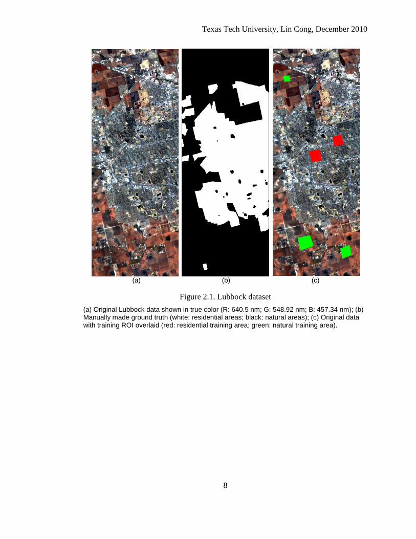
(a) (b)
Figure 2.3. An example of destriping (a) Band 119 (1336.15 nm) before vertical destriping; (b) Band 119 after vertical destriping.
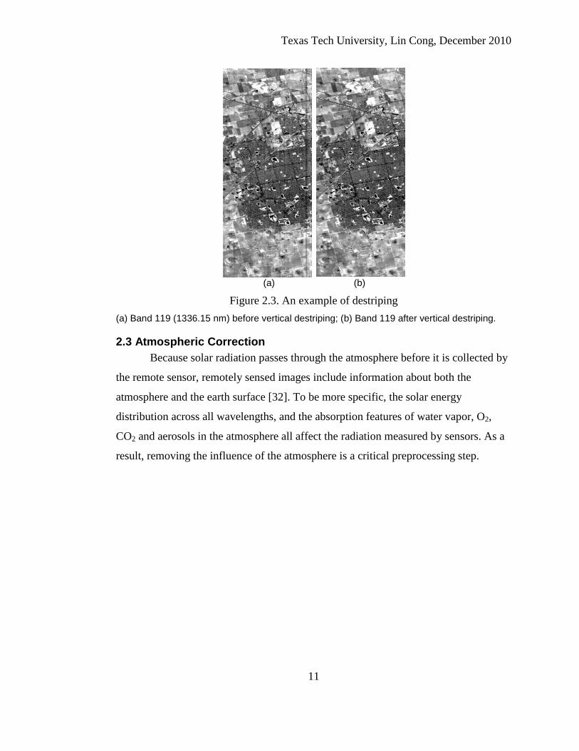
2.3 Atmospheric Correction Because solar radiation passes through the atmosphere before it is collected by
the remote sensor, remotely sensed images include information about both the
atmosphere and the earth surface [32]. To be more specific, the solar energy
distribution across all wavelengths, and the absorption features of water vapor, O2,
CO2 and aerosols in the atmosphere all affect the radiation measured by sensors. As a
result, removing the influence of the atmosphere is a critical preprocessing step.
Texas Tech University, Lin Cong, December 2010
12
(a)
(b)
Figure 2.4. Solar energy distribution and atmospheric absorption (a) Solar spectrum, image courtesy of [33]; (b) Atmosphere transmittance, image courtesy of [34].
The FLAASH module developed by Spectral Sciences, Inc., in collaboration
with the U.S. Air Force Research Laboratory (AFRL) and Spectral Information
Technology Application Center (SITAC) was applied in this project to compensate for
atmosphere effects.
Texas Tech University, Lin Cong, December 2010
13
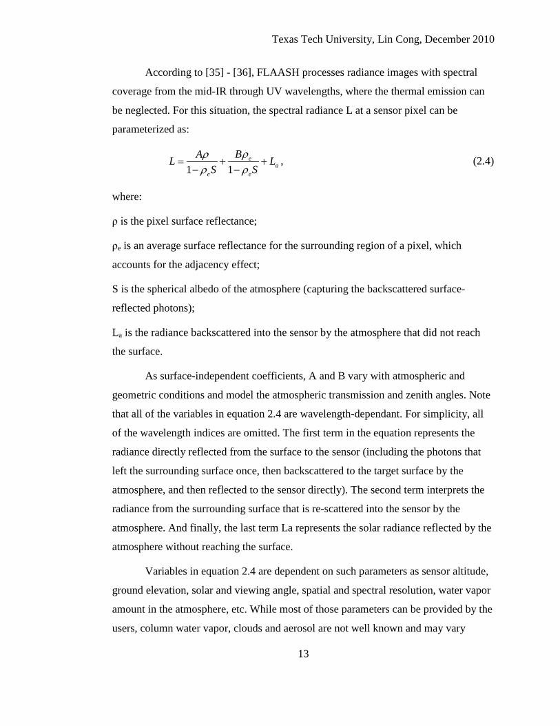
According to [35] - [36], FLAASH processes radiance images with spectral
coverage from the mid-IR through UV wavelengths, where the thermal emission can
be neglected. For this situation, the spectral radiance L at a sensor pixel can be
parameterized as:
1 1
ea
e e
BAL LS S
ρρρ ρ
= + +− −
, (2.4)
where:
ρ is the pixel surface reflectance;
ρe is an average surface reflectance for the surrounding region of a pixel, which
accounts for the adjacency effect;
S is the spherical albedo of the atmosphere (capturing the backscattered surface-
reflected photons);
La is the radiance backscattered into the sensor by the atmosphere that did not reach
the surface.
As surface-independent coefficients, A and B vary with atmospheric and
geometric conditions and model the atmospheric transmission and zenith angles. Note
that all of the variables in equation 2.4 are wavelength-dependant. For simplicity, all
of the wavelength indices are omitted. The first term in the equation represents the
radiance directly reflected from the surface to the sensor (including the photons that
left the surrounding surface once, then backscattered to the target surface by the
atmosphere, and then reflected to the sensor directly). The second term interprets the
radiance from the surrounding surface that is re-scattered into the sensor by the
atmosphere. And finally, the last term La represents the solar radiance reflected by the
atmosphere without reaching the surface.
Variables in equation 2.4 are dependent on such parameters as sensor altitude,
ground elevation, solar and viewing angle, spatial and spectral resolution, water vapor
amount in the atmosphere, etc. While most of those parameters can be provided by the
users, column water vapor, clouds and aerosol are not well known and may vary
Texas Tech University, Lin Cong, December 2010
14
across the scene. FLAASH first retrieves preliminary column water vapor on a pixel-
by-pixel basis. For simplicity, the adjacency effect is ignored in this step, so that ρe
and ρ are taken as equal in equation 2.4. The basis of the retrieval algorithm is the
strong correlation of column water vapor and the ratio of reference radiance (the
shoulders of the water absorption band) to absorption radiance (center of the same
water absorption band) [31]. MODTRAN4 radiation transfer code incorporated within
FLAASH generates values of A+B, S and La for different column water vapor at
reference and absorption wavelengths. Then, a set of reference and absorption
radiances L are simulated for a series of reflectances (0, 0.01, 0.02, … 0.99, 1). The
results are transformed into a 2-dimensional Look-Up Table (LUT), for which the
reference radiance and ratio are the two independent variables, and the water vapor is
the dependent variable. This 2-dimensional LUT is then searched to retrieve the
column water vapor for each pixel.
Cirrus or other kinds of high altitude clouds are identified by using radiance
around the 1.38 um water absorption band [31]. Under clear sky conditions, this band
is very dark, because most of its photons are absorbed by water vapor when they
traverse the atmosphere. However, when high altitude clouds are present, photons do
not complete the full path through the atmosphere. Instead, they are reflected to the
sensor by the clouds before they can be absorbed. As a result, the radiances around
1.38 um are used in FLAASH to detect cirrus, and the cloud pixels are removed when
the adjacency effect is analyzed in the next step.
FLAASH convolves the data cube with a point spread function to describe the
photons reflected from adjacent pixels and scattered to the sensor by atmosphere.
Currently, FLAASH assumes that the point spread function is a modified radial
exponential function, independent of wavelength. The result is a new data cube of
spatially convolved spectral radiance Le. Then, ρe can be approximately solved by
equation 2.5.
( )1
ee a
e
A BL LSρ
ρ+
= +−
(2.5)

Texas Tech University, Lin Cong, December 2010
15
After the column water vapor retrieval, variables such as A, B, S and La are
generated from the MODTRAN radiation simulation. Then, average surface
reflectance ρe can be solved from equation 2.5 using the above variables and Le from
the spatially convolved radiance image. Finally, reflectance ρ can be solved for each
band of each pixel by equation 2.4. Because the FLAASH module is built in the
ENVI© software package, it can be implemented easily given that all the parameters
required by the software are provided correctly. For more detailed information of the
FLAASH algorithm, please refer to [35] - [39].
(a) (b)
(c) (d)
Figure 2.5. Radiance versus reflectance of some major materials from the image (a) Relatively pure soil; (b) Relatively pure vegetation; (c) Relatively pure road; (d) A mixture of vegetation, construction material and soil from a residential neighborhood. Yellow: radiance; White: reflectance.
2.4 Chapter Conclusions The preprocessing of the Hyperion hyperspectral data was explained in this
chapter. In the first step, histogram normalization was implemented to remove the

Texas Tech University, Lin Cong, December 2010
16
visual stripes caused by different sensitivity of specific pushbroom sensors. In the
second step, the FLAASH algorithm was applied to compensate for the atmospheric
absorption effect and convert the measured radiance to the reflectance that is
necessary for the material recognition in the following procedures. After the two steps
of preprocessing, the resulting data was ready for spectral-spatial feature extraction in
Chapter III.

Texas Tech University, Lin Cong, December 2010
17
CHAPTER III
FEATURE EXTRACTION In this chapter, a method of spectral – spatial feature extraction from low
resolution Hyperion data is explained. In general, the spectral feature elements will
derive from the spectral similarity of each pixel with man-made material endmembers
or spectrum of each pixel in a reduced dimensional space. A hierarchical Fourier
transform – co-occurrence matrix method is designed and implemented within the
sliding window centered at each pixel. Eight second order texture measures are
calculated based on the co-occurrence matrix, and K-fold cross validation is
performed on the training data to select the best combination of features for the
proposed joint solution.
3.1 Spectral Feature Extraction
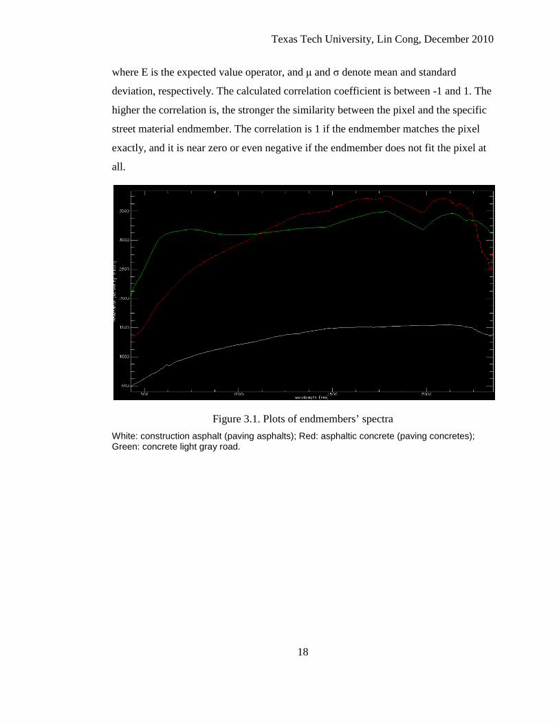
3.1.1 Normalized Correlation Based on the prior knowledge that most roads in Lubbock are built from
asphalt or concrete with only a few exceptions built from bricks, the normalized
correlation of a pixel’s spectrum against asphalt and/or concrete spectra is used as the
measurement of spectral similarity of the pixel to manmade materials. Because streets
are less than one pixel wide in the low resolution Hyperion data, extraction of pure
construction material from the data is extremely difficult. Instead, three different
asphalt and concrete spectra are selected from the USGS digital spectral library
(speclib06a [40]) as endmembers. Spectral plots of these three endmembers are shown
in Fig. 3.1.
Let xij denote spectrum at position (i, j) and yk denote spectrum of endmember
k. The normalized correlation coefficient at position (i, j) against endmember k is
defined as:
,
,
,, ,
[( )( )]i j k
i j k
i j x k yi j k
x y
E x yc
µ µ
σ σ
− −= , (3.1)
Texas Tech University, Lin Cong, December 2010
18
where E is the expected value operator, and μ and σ denote mean and standard
deviation, respectively. The calculated correlation coefficient is between -1 and 1. The
higher the correlation is, the stronger the similarity between the pixel and the specific
street material endmember. The correlation is 1 if the endmember matches the pixel
exactly, and it is near zero or even negative if the endmember does not fit the pixel at
all.
Figure 3.1. Plots of endmembers’ spectra White: construction asphalt (paving asphalts); Red: asphaltic concrete (paving concretes); Green: concrete light gray road.
Texas Tech University, Lin Cong, December 2010
19
(a) (b) (c)
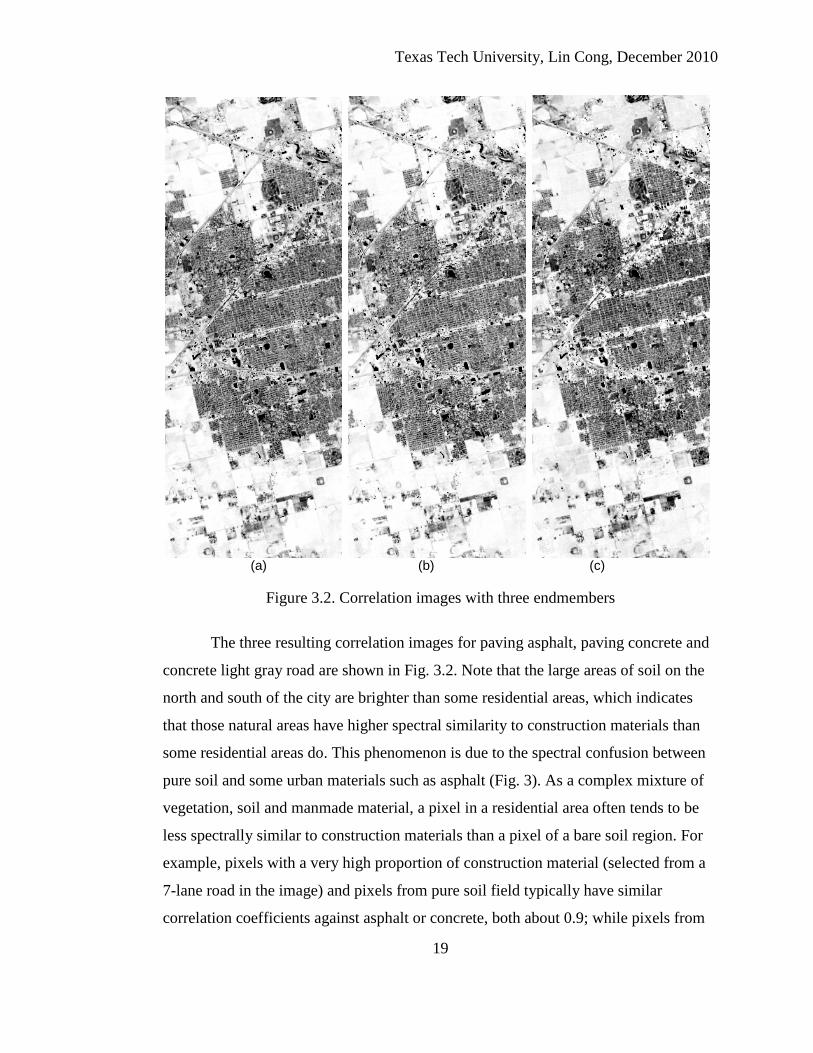
Figure 3.2. Correlation images with three endmembers
The three resulting correlation images for paving asphalt, paving concrete and
concrete light gray road are shown in Fig. 3.2. Note that the large areas of soil on the
north and south of the city are brighter than some residential areas, which indicates
that those natural areas have higher spectral similarity to construction materials than
some residential areas do. This phenomenon is due to the spectral confusion between
pure soil and some urban materials such as asphalt (Fig. 3). As a complex mixture of
vegetation, soil and manmade material, a pixel in a residential area often tends to be
less spectrally similar to construction materials than a pixel of a bare soil region. For
example, pixels with a very high proportion of construction material (selected from a
7-lane road in the image) and pixels from pure soil field typically have similar
correlation coefficients against asphalt or concrete, both about 0.9; while pixels from

Texas Tech University, Lin Cong, December 2010
20
neighborhood blocks, which contain relatively high percentage of vegetation, usually
just have a correlation value between 0.3 and 0.7 against those construction materials.
Thus, a single pixel is difficult to classify by only using spectrum, especially in pixel
level classification. However, if many spectrally similar pixels are identified in a line
or even in a grid pattern, the likelihood of streets becomes high. Thus, macroscopic
spatial texture is desired for accurate residential area classification, especially for low
resolution hyperspectral images.
3.1.2 Principal Component Analysis (PCA) PCA is a mathematical procedure that transforms a number of possibly
correlated variables into a smaller number of uncorrelated variables called principal
components. The first principal component accounts for as much of the variability in
the data as possible, and each succeeding component accounts for as much of the
remaining variability as possible [41]. The most significant components are selected to
serve as spectral features.
The first step of PCA is to calculate the covariance matrix as follows:
1
1cov ( ) ( )N
ti i
ix u x u
N =
= − × −∑ , (3.2)
where ix denotes any spectrum vector and u denotes the mean value vector of all
spectra. The covariance matrix is the average of outer product matrices of spectral
samples. In the second step, eigenvalues of the covariance matrix are calculated and
sorted in descending order. The transform matrix (T) is formed by concatenating
transposed eigenvectors ( tie ) row by row in the same order as the eigenvalues. Finally,
all the spectra are transformed into PCA space by left-multiplying the transform
matrix as in equation 3.3.
1
* 2
...
t
t
i i i
tl
ee
x T x x
e
= ⋅ = ⋅
(3.3)

Texas Tech University, Lin Cong, December 2010
21
Subscript l in equation 3.3 represents the dimensionality of new data, which depends
on the number of eigenvectors used to build the transform matrix. Generally, PCA is
used to reduce the dimensionality of spectral data, while, at the same time, keeping as
much information as possible.
Because the New Orleans dataset contains large areas of river and the spectral
difference between water and other materials are more dramatic than the difference
between construction and natural materials, the first few principle components tend to
be dominated by the large spectral variance between water and other materials. In
order to make the PCA transform more sensitive to the spectral variance between
construction and natural materials, water pixels are detected and labeled as “water”,
then the remaining pixels are PCA transformed. After classification, the “water”
segmentation is merged back into the “natural” class.
Based on the distinct spectral signature of water, such as the reflectance peak
at about 548 nm (green band) and the near-zero reflectance at about 1205 nm, which is
very different from most other materials, an algorithm similar to Normalized
Difference Vegetation Index (NDVI) is designed to assess whether the target is (or
contains) liquid water or not. The water index is defined in equation 3.4. By definition,
the water index is a scalar between -1 and 1, unless the NIR band around 1205 nm is
very noisy and the reflectance is negative, which does happen in a rare case. Generally
the higher the index value is, the higher the possibility that the target has liquid water.
In practice, 0.5 has been found as a reliable threshold between water and non-water.
The water mask built for the New Orleans dataset is shown in Fig. 3.4a.
GREEN NIRwater indexGREEN NIR
−=
+ (3.4)

Texas Tech University, Lin Cong, December 2010
22
Figure 3.3. Plot of eigenvalues of New Orleans data
Table 3.1. Cumulative percentage of variance for top few principal components of New Orleans data
Principal Component
Index
Ordinary PCA Water-removed PCA
1 72.56% 59.79% 2 96.82% 94.34% 3 98.63% 97.54% 4 99.08% 98.36% 5 99.26% 98.70%
In Fig. 3.3, for both PCA transforms, each of the first two principal bands has
at least 10 times stronger variance than all the other components. As shown in Table
3.1, the cumulative percentage of variance of the first two components is around 95%,
which means that the combination of the first two principal components is a good
representation of the complete dataset. By comparing Fig. 3.4b and 3.4c, one can
observe that the first component image of the water-removed PCA transform has a
higher visual contrast between residential areas and natural areas than the first
component image of the traditional PCA transform. Furthermore, as shown in the
histograms of the first bands of the ordinary PCA and the water-removed PCA
0 20 40 60 80 100 120 140 1607
8
9
10
11
12
13
14
principle component index
log1
0 of
eig
enva
lues
water removed PCAordinary PCA
Texas Tech University, Lin Cong, December 2010
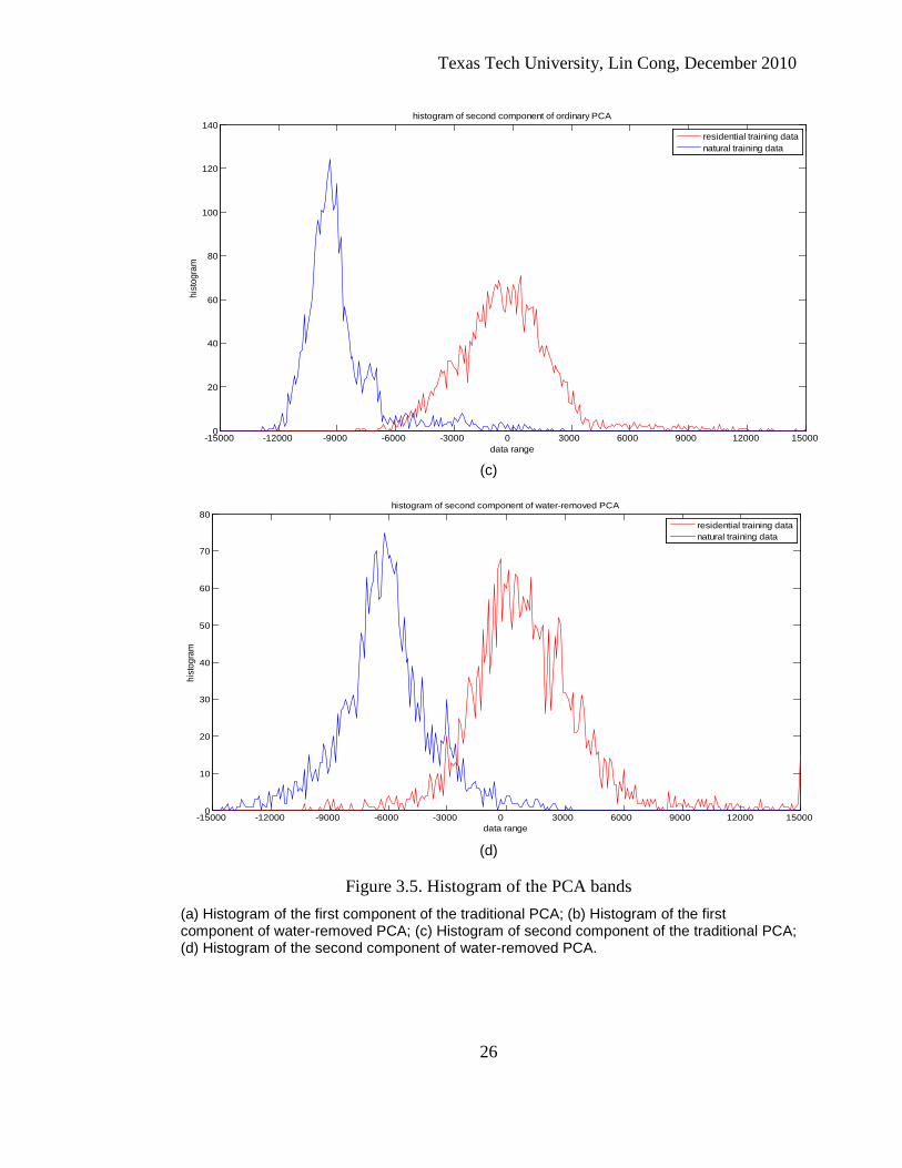
23
transform (Fig. 3.5a and 3.5b), the peak of the residential training data and the peak of
the natural training data coincide for the ordinary PCA transform, but well separate for
the water-removed PCA transform. The second bands of both PCA transforms have
similar separability as shown in Fig. 3.5c and 3.5d. According to the comparison
between the histograms, the conclusion that water-removed PCA transform generates
preferable spectral features to the traditional PCA transform can be made.
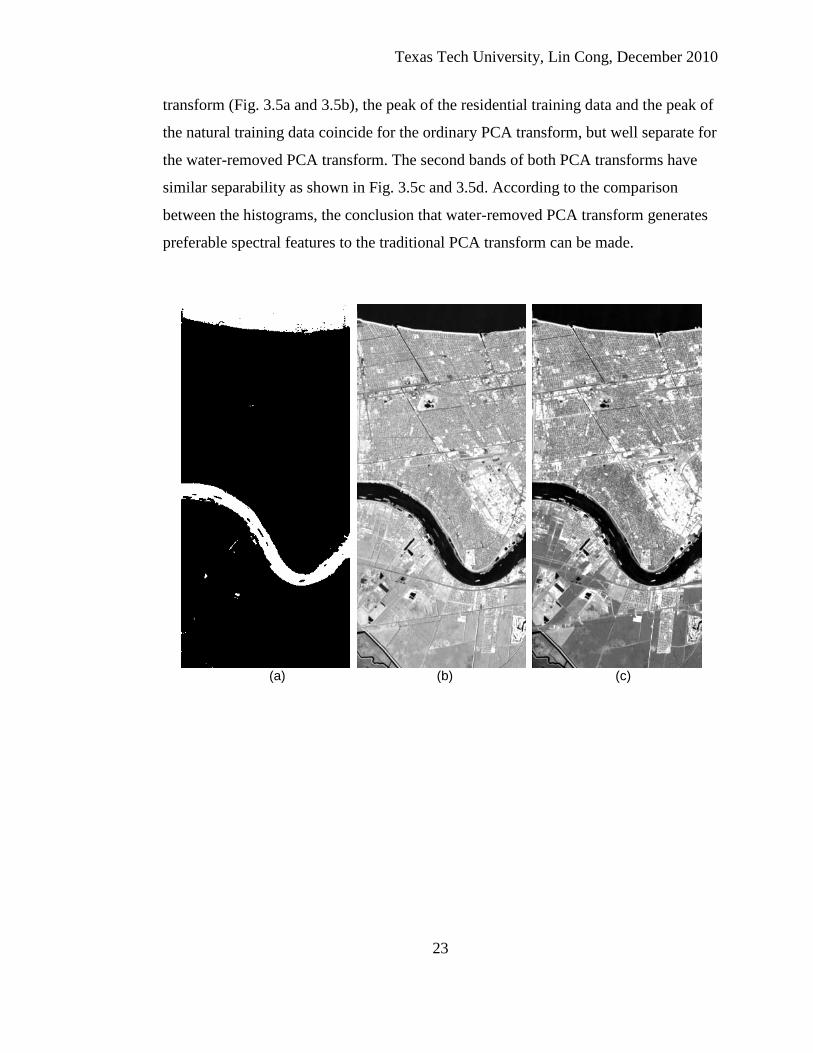
(a) (b) (c)

Texas Tech University, Lin Cong, December 2010
24
(d) (e)
Figure 3.4. PCA results of New Orleans dataset (a) Water mask; (b) The first band of the traditional PCA transform; (c) The first band of water-removed PCA transform; (d) The second band of the traditional PCA transform; (e) The second band of water-removed PCA transform.

Texas Tech University, Lin Cong, December 2010
25
(a)
(b)
-15000 -12000 -9000 -6000 -3000 0 3000 6000 9000 12000 15000 0
10
20
30
40
50
60
70
80
90histogram of first component of ordinary PCA
data range
hist
ogra
m
residential training datanatural training data
-15000 -12000 -9000 -6000 -3000 0 3000 6000 9000 12000 15000 0
20
40
60
80
100
120
140
160
180
200
data range
hist
ogra
m
histogram of first component of water-removed PCA
residential training datanatural training data
Texas Tech University, Lin Cong, December 2010
26
(c)
(d)
Figure 3.5. Histogram of the PCA bands (a) Histogram of the first component of the traditional PCA; (b) Histogram of the first component of water-removed PCA; (c) Histogram of second component of the traditional PCA; (d) Histogram of the second component of water-removed PCA.
-15000 -12000 -9000 -6000 -3000 0 3000 6000 9000 12000 15000 0
20
40
60
80
100
120
140
data range
hist
ogra
m
histogram of second component of ordinary PCA
residential training datanatural training data
-15000 -12000 -9000 -6000 -3000 0 3000 6000 9000 12000 15000 0
10
20
30
40
50
60
70
80
data range
hist
ogra
m
histogram of second component of water-removed PCA
residential training datanatural training data

Texas Tech University, Lin Cong, December 2010
27
3.1.3 Comparison of Normalized Correlation and PCA Two alternative spectral feature extraction methods used in this study were
introduced in the previous two sections. Generally, both methods have pros and cons.
In this section, a detailed comparison between the two methods is presented.
The advantage of the correlation method is that as a measurement of spectral
similarity, the value of normalized correlation coefficient is proportional to the degree
to which the pixel is spectrally similar to the endmember. In theory, the residential
areas have higher spectral similarity to construction materials than natural areas do,
and as a result, the correlation value should be larger in residential areas than in
natural areas. To this extent, the correlation coefficient has a clearer physical meaning
as a spectral feature than PCA components do. However, the correlation method
requires prior knowledge about the prevailing man-made materials in the study site,
which is sometimes not easily available. Furthermore, considering the coarse spatial
resolution, the physical meaning of correlation coefficient may be undermined by the
spectral confusion between soil and neighborhood mixture, as explained in section
3.1.1.
On the other hand, the PCA method does not require prior knowledge of road
materials and is able to efficiently reduce the volume of the dataset based on the
inherent structure of the data. However, the PCA transform is not discrimination-
oriented. Sometimes, just having the largest variance does not mean that the particular
direction is the best suited to classify different clusters. It is possible that the directions
discarded by PCA might be exactly the directions that are required to distinguish
between classes. One of these awkward cases is described in [42]. PCA might
discover, for example, the gross features that characterize (uppercase letters) Os and
Qs, but might ignore the tail that distinguishes an O from a Q. Similarly, in presence
of large areas of water pixels or reflectance-saturated pixels, the huge spectral
difference between water (or saturated) pixels and the other pixels is characterized as
the gross features by the traditional PCA transform, and the difference between
residential and natural pixels is characterized as less important features. By removing

Texas Tech University, Lin Cong, December 2010
28
the water pixels before calculating the covariance matrix, the performance of PCA
transform can be improved to some extent.
In this thesis, correlation coefficients and PCA components are both used to
extract spectral information from the Lubbock dataset and the New Orleans dataset.
3.2 Spatial Feature Extraction The selected datasets represent two different styles of city arrangement. The
city of Lubbock is built on clear grid patterns and is relatively easy to distinguish from
the surrounding rural areas. The city of New Orleans is less structured: the streets and
avenues are not orthogonal to each other, and the direction of roads varies from
neighborhood to neighborhood. The complexity of urban arrangement in New Orleans
makes the classification quite challenging but not impossible. To capture the periodic
textures oriented in different directions in different neighborhoods, a hierarchical
Fourier Transform – Co-occurrence Matrix approach is developed. The Fourier
transform is first implemented to detect the angle of local periodic texture, and the co-
occurrence matrix is calculated with the dominant angle detected from the Fourier
transform. Finally, spatial features are extracted from a series of second order texture
measures calculated from co-occurrence matrices. Both the Fourier transform and the
co-occurrence matrix are calculated on a sliding window basis, and the extracted
spatial features are assigned to the center pixel of the window.
3.2.1 Hierarchical Fourier Transform – Co-occurrence Approach 1. Two-dimensional Fourier Transform
The two-dimensional Fourier transform (FT) is defined as equation 3.5 and
3.6:
1 1 2 ( )
0 0
1[ , ] [ , ]mk nlN M jM N
n mF k l f m n e
MNπ− − − +
= =
= ×∑∑ , and (3.5)
1 1 2 ( )
0 0
1[ , ] [ , ]mk nlN M jM N
l kf m n F k l e
MNπ− − +
= =
= ×∑∑ , (3.6)

Texas Tech University, Lin Cong, December 2010
29
where f denotes the original image and F denotes the Fourier image. M and N are the
dimensions of original and transformed images. Every component in the Fourier
domain, i.e. F[k,l], represents the magnitude and phase of the 2D harmonic wave, with
frequency of k in one dimension and frequency of l in the other dimension. For our
study images and typical road spacing, a tile of 31-by-31 to 51-by-51 is found
appropriate for reliable detection in the Fourier analysis. If the tile is too large, it tends
to cover both residential and nonresidential areas; if the tile is too small, the Fourier
components associated with grid patterns tend to be close to DC and are vulnerable to
misclassification as low frequency components. In practice, a 41-by-41 tile is used for
all applications.
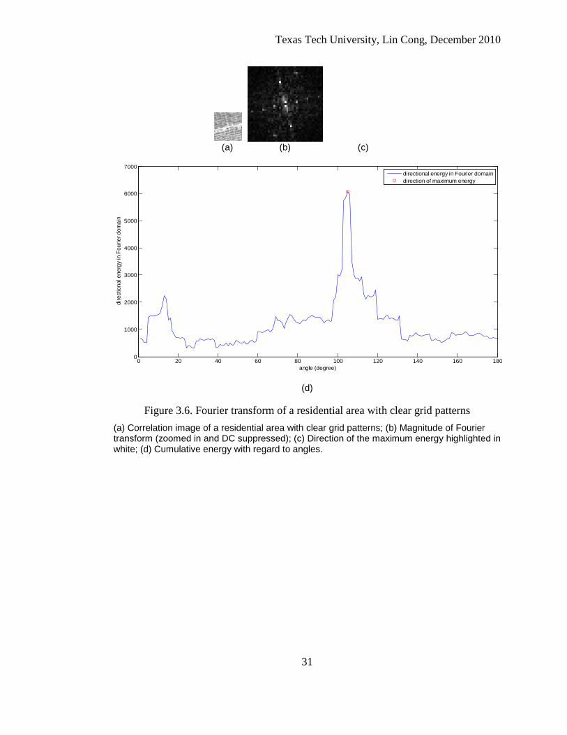
Figs. 3.6 - 3.10 demonstrate the Fourier transforms of three out of many types
of residential regions and two out of many types of natural regions in both Lubbock
and New Orleans datasets. For a clear grid pattern (Fig. 3.6), the FT components
associated with the periodic street patterns have large magnitudes, shown as very
bright pixels in Fig. 3.6b. The relationship between a spatial pattern and its Fourier
components is that all the associated components are aligned orthogonal to the spatial
pattern. If the gray level changes following an approximate sinusoidal pattern, most of
the energy will be concentrated into a few single components, and the distance from
those strong components to the origin indicates the number of periods that the spatial
pattern has within the tile. On the other hand, because no periodic pattern exists in the
natural region, the peak Fourier components are very close to the origin, as shown in
Fig. 3.9b and Fig. 3.10b. Based on the difference in the Fourier domain, the position of
peak FT components was initially designed as the spatial feature of the center pixel of
the tile.
However, for the residential region shown in Fig. 3.7, where the existence of
lakes interrupts the periodic spatial pattern, many low frequency components are
stronger than or at least comparable to the actual components associated with the street
spacing (Fig. 3.7b). For the residential areas, where more than one kind of street
pattern exists in the tile, as shown in Fig. 3.8, it is almost impossible to use a pair of
Fourier components to represent the spatial pattern, or in other words to use the

Texas Tech University, Lin Cong, December 2010
30
position of a single peak component as an effective spatial feature for the center pixel
of the tile. Even if a single peak Fourier component is not always trustworthy, the
direction of the strongest cumulative energy in Fourier domain is usually consistent
with the direction of the street pattern (subimage c and d of Fig. 3.6 – 3.10). Because
the strongest direction is more noise tolerant than strongest component, a more
complex algorithm combining the detected direction and co-occurrence matrix has
been designed.
Texas Tech University, Lin Cong, December 2010
31
(a) (b) (c)
(d)
Figure 3.6. Fourier transform of a residential area with clear grid patterns (a) Correlation image of a residential area with clear grid patterns; (b) Magnitude of Fourier transform (zoomed in and DC suppressed); (c) Direction of the maximum energy highlighted in white; (d) Cumulative energy with regard to angles.
0 20 40 60 80 100 120 140 160 1800
1000
2000
3000
4000
5000
6000
7000
angle (degree)
dire
ctio
nal e
nerg
y in
Fou
rier d
omai
n
directional energy in Fourier domaindirection of maximum energy

Texas Tech University, Lin Cong, December 2010
32
(a) (b) (c)
(d)
Figure 3.7. Fourier transform of a residential area containing lakes (a) Correlation image of a residential area containing lakes; (b) Magnitude of Fourier transform (zoomed in and DC suppressed); (c) Direction of the maximum energy highlighted in white; (d) Cumulative energy with regard to angles.
0 20 40 60 80 100 120 140 160 1800
2000
4000
6000
8000
10000
12000
angle (degree)
ener
gy
directional energy spectrumdirection of the maximum engergy

Texas Tech University, Lin Cong, December 2010
33
(a) (b) (c)
(d)
Figure 3.8. Fourier transform of a disordered residential (a) PCA image (1st band) of a disordered residential area in the city of New Orleans; (b) Magnitude of Fourier transform (zoomed in and DC suppressed); (c) Direction of the maximum energy highlighted in white; (d) Cumulative energy with regard to angles.
0 20 40 60 80 100 120 140 160 1800
0.2
0.4
0.6
0.8
1
1.2
1.4
1.6
1.8
2
2.2x 10
12
angle (degree)
ener
gy
directional energy spectrumdirection of the maximum energy

Texas Tech University, Lin Cong, December 2010
34
(a) (b) (c)
(d)
Figure 3.9. Fourier transform of a nonresidential region (a) PCA image (1st band) of a nonresidential region; (b) Magnitude of Fourier transform (zoomed in and DC suppressed); (c) Direction of the maximum energy highlighted in white; (d) Cumulative energy with regard to angles.
0 20 40 60 80 100 120 140 160 1800.2
0.4
0.6
0.8
1
1.2
1.4
1.6
1.8
2x 10
11
angle (degree)
dire
ctio
nal e
nerg
y in
Fou
rier d
omai
n
directional energy in Fourier domaindirection of the maximu energy

Texas Tech University, Lin Cong, December 2010
35
(a) (b) (c)
(d)
Figure 3.10. Fourier transform of a grassland region with a country road (a) PCA image (1st band) of a grassland region with a country road; (b) Magnitude of Fourier transform (zoomed in and DC suppressed); (c) Direction of the maximum energy highlighted in white; (d) Cumulative energy with regard to angles.
0 20 40 60 80 100 120 140 160 1800
1
2
3
4
5
6
7x 10
11
angle (degree)
ener
gy
directional engergy spectrumdirection of the maximum energy

Texas Tech University, Lin Cong, December 2010
36
2. Co-occurrence matrix
A co-occurrence matrix is a matrix that is defined over an image to be the
distribution of co-occurring gray levels at a given offset between the reference and the
neighboring pixels. First proposed by Haralick et al. in 1970s [43], the co-occurrence
matrix (aka gray-level co-occurrence matrix) is defined as equation 3.7 and 3.8:
,1 1
1, ( , ) & ( , )( , ) ( , ) & ( , )
0,
n m
x yp q
if I p q i I p x q y j orC i j if I p q j I p x q y i
otherwise∆ ∆
= =
= + ∆ + ∆ == = + ∆ + ∆ =
∑∑ , and (3.7)
,,
,,
( , )( , )
( , )x y
x yx y
i j
C i jP i j
C i j∆ ∆
∆ ∆∆ ∆
=∑
, (3.8)
where i and j denote the quantized gray levels; I, C and P denote the original image
(matrix), the framework matrix and the co-occurrence matrix, respectively; x∆ and
y∆ denote the offset between the reference and the neighbor pixels. The difference
between the framework matrix and the co-occurrence matrix is that the entries of the
framework matrix are the counts of co-occurring gray levels, while the entries of the
final co-occurrence matrix are normalized to the probabilities. By definition, co-
occurrence matrices are always symmetric square matrices, and the size is dependent
on the quantization levels.
In place of offset ( x∆ , y∆ ), a displacement and angle are often used to
describe the relationship between the reference and the neighbor pixels. In order to
achieve rotational invariance, four co-occurrence matrices were usually calculated
based on the same displacement in four orthogonal angles (i.e. 0o, 45o, 90o and 135o to
the horizontal right) [27], then the texture measures derived from different co-
occurrence matrices are averaged. The approach of calculating four co-occurrence
matrices in four orthogonal angles was called the omnidirectional method. Rather than
using the omnidirectional method, the angle in our study is determined by the prior
Fourier analysis, and the displacement is set as 1 for all applications, based on the
street spacing. Compared with the omnidirectional method, the angle of maximum
Texas Tech University, Lin Cong, December 2010
37
energy in the Fourier domain is more desirable, because that angle should be
orthogonal to the periodic street patterns, and the neighboring pixels in that angle
should have the largest contrast, and, at the same time, the angle from Fourier analysis
is also rotationally invariant. The omnidirectional method, on the other hand, includes
both correct and incorrect directions and the spatial features extracted, as an average
of four, is not as sharp as those extracted by using angles from Fourier analysis.
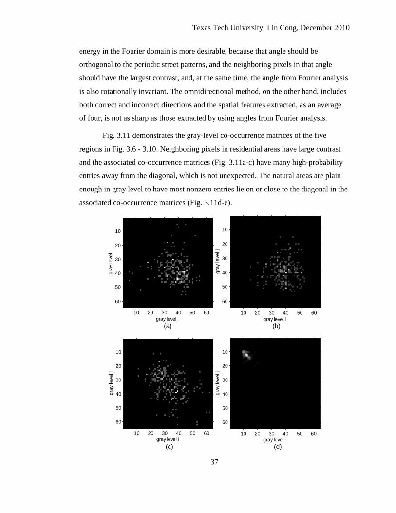
Fig. 3.11 demonstrates the gray-level co-occurrence matrices of the five
regions in Fig. 3.6 - 3.10. Neighboring pixels in residential areas have large contrast
and the associated co-occurrence matrices (Fig. 3.11a-c) have many high-probability
entries away from the diagonal, which is not unexpected. The natural areas are plain
enough in gray level to have most nonzero entries lie on or close to the diagonal in the
associated co-occurrence matrices (Fig. 3.11d-e).
(a) (b)
(c) (d)
gray level i
gray
leve
l j
10 20 30 40 50 60
10
20
30
40
50
60
gray level i
gray
leve
l j
10 20 30 40 50 60
10
20
30
40
50
60
gray level i
gray
leve
l j
10 20 30 40 50 60
10
20
30
40
50
60
gray level i
gray
leve
l j
10 20 30 40 50 60
10
20
30
40
50
60

Texas Tech University, Lin Cong, December 2010
38
(e)
Figure 3.11. Co-occurrence matrices of the five example regions (a) Co-occurrence matrix of the residential area with clear grid patterns; (b) Co-occurrence matrix of the residential area containing lakes; (c) Co-occurrence matrix of the disordered residential area with more than one street structure; (d) Co-occurrence matrix of the nonresidential area; (e) Co-occurrence matrix of the grassland region with a country road.
3.2.2 Texture Measures The co-occurrence matrix is used for a series of second order texture
calculations. The difference between first order and second order texture measures is
that the first order measures are statistics calculated from the original image, such as
mean and variance, and do not consider pixel neighborhood relationships, while the
second order measures consider the relationship between groups of two pixels in the
original image and are usually calculated from a co-occurrence matrix [44]. According
to the purpose, texture measures can be divided into three general groups: contrast
group, orderliness group and statistics group.
Generally, the texture measures are weighted averages of cell contents of a co-
occurrence matrix. The contrast group focuses on the contrast between neighboring
pixels in the original image and creates weights for each entry of the co-occurrence
matrix so that the resulting measures are larger (or smaller in some measures) where a
stronger contrast exists. Because entries on the diagonal in a co-occurrence matrix
represent no contrast, and contrast increases away from the diagonal, measures in this
group create an increasing (or decreasing in some measures) weight as the distance
from the diagonal increases. The orderliness group measures how regular (orderly) the
gray level i
gray
leve
l j
10 20 30 40 50 60
10
20
30
40
50
60

Texas Tech University, Lin Cong, December 2010
39
pixel values are within the sliding window. Generally an orderly image has most of the
probability concentrated in a few entries in the co-occurrence matrix, while a
disorderly image has the probability almost evenly distributed across a number of
entries. Thus, measures in this group create a weight increasing (or decreasing in some
measures) with the commonness of the gray level co-occurring combination. The
statistics group calculates the mean, variance, correlation etc. of the co-occurrence
matrix [44].
(1) Contrast (CON)
2,
, 1( )
N
i ji j
CON P i j=
= −∑ (3.10)
The weights are second norm of the gray level difference between two
neighboring pixels. The higher the contrast measure is, the higher contrast the image
has. A simple image window will have a contrast measure approaching 0.
(2) Dissimilarity (DIS)
,, 1
N
i ji j
DIS P i j=
= −∑ (3.11)
The weights are the first norm of the gray level difference between
neighboring pixels. A simple image window will have a contrast measure approaching
0.
(3) Homogeneity (HOM)
,2
, 11 ( )
Ni j
i j
PHOM
i j=
=+ −∑ (3.12)
The weights are inverse second norm of the gray level difference between two
neighboring pixels. The value of homogeneity is between 0 and 1, with 1 for a
perfectly plain window and close to 0 for a sharply contrasted window.
(4) Similarity (SIM)
Texas Tech University, Lin Cong, December 2010
40
,
, 11
Ni j
i j
PSIM
i j=
=+ −∑ (3.13)
The weights are inverse first norm of the gray level difference between two
neighboring pixels. The value of homogeneity is between 0 and 1, with 1 for a
perfectly plain window and close to 0 for a sharply contrasted window.
(5) Angular Second Moment (ASM)
2,
, 1
N
i ji j
ASM P=
= ∑ (3.14)
The weight of an entry’s content (probability) is the probability itself. The
value of ASM is between 0 and 1, and high values occur when the window is orderly.
The reason why a higher value of ASM indicates a more orderly image is simply (but
not strictly) interpreted as follows:
Assume that there are N quantized gray levels and hence N2 entries in the co-
occurrence matrix. The summation of probabilities is always 1:
, ,1 1
1, 0N N
i j i ji j
P where P= =
= ≥∑∑ . (3.15)
If both sides of (3.15) are squared, (3.16) can be found:
2 2, , , ,
1 1 1 1 , 1 , 1( ) 1 1 2
N N N N N N
i j i j i j m ni j i j i j m n
m i orn j
P P P P= = = = = =
≠≠
= ⇔ = −∑∑ ∑∑ ∑ ∑ . (3.16)
The following inequality is always true based on the Cauchy-Schwarz theorem:
2 2, , , , , ,2 , 0, 0.i j m n i j m n i j m nP P P P where P P≤ + ≥ ≥ (3.17)
The equality in (3.17) occurs if and only if:
, , , 1 ( , ) ,1 ( , ) ,i j m nP P i j N m n N m i or n j= ∀ ≤ ≤ ≤ ≤ ≠ ≠ .
Through some simple mathematical calculations, the following inequality can be
found from equation 3.16:

Texas Tech University, Lin Cong, December 2010
41
2 2 2, ,
1 1 1 11 1 ( 1)
N N N N
i j i ji j i j
P N P= = = =
≥ ≥ − − ⇔∑∑ ∑∑
2, 2
1 1
11N N
i ji j
PN= =
≥ ≥∑∑ , (3.18)
where the maximum of ASM will be found if and only if exactly one entry of the co-
occurrence matrix is 1 and all the other entries are 0; the minimum of ASM will be
found if and only if all the entries contain the same probability 2
1N
.
With repetitive spatial patterns, an orderly image tends to have most of the
probability concentrated in only a few entries of the co-occurrence matrix while
leaving all the other entries approaching 0, and the ASM is close to 1 as a result. On
the other hand, with different spatial patterns here and there, a disorderly image tends
to have the probability almost evenly distributed across a number of entries, which
results in a relatively small value of ASM.
(6) Maximum Probability (MAX)
,max( )i jMAX P= (3.19)
Having most of the probability concentrated in only a few entries of co-
occurrence matrix, an orderly image will have a relatively large value of MAX. A
disorderly image, on the other hand, having the probability almost evenly distributed
across many entries, will have a relatively small value of MAX.
(7) Entropy (ENT)
, 2 ,, 1
logN
i j i ji j
ENT P P=
= −∑ (3.20)
Here, we must assume that 20 log 0 0× = . As the name suggests, entropy is a
measure of disorder. It is 0 if the window is perfectly orderly and is larger for a more
disorderly window.
(8) Co-occurrence matrix Correlation (COR)
Texas Tech University, Lin Cong, December 2010
42
,
, 1
,, 1
( )
( )
N
i i ji j
N
j i ji j
i P
j P
µ
µ
=
=
=
=
∑
∑ (3.21)
2 2,
, 1
2 2,
, 1
( )
( )
N
i i j ii j
N
j i j ji j
P i
P j
σ µ
σ µ
=
=
= −
= −
∑
∑ (3.22)
,, 1
( )( )Ni j
i ji j i j
i jCOR P
µ µσ σ=
− −= ∑ (3.23)
COR measures the linear dependency of gray levels between neighboring
pixels. Intuitively, 0 means uncorrelated and 1 means perfectly correlated.
3.2.3 Separability Assessment of Texture Measures In order to further analyze the separability of all the eight texture measures,
two classes of testing data are selected from each dataset, as shown in Fig. 3.12. Note
that some imperfect testing data is deliberately selected, i.e. residential areas with
weak periodic patterns and natural areas with low uniformity because of country roads
or small houses. Fisher’s discriminant ratio is calculated, for each texture, as a
measurement of separability between residential and natural areas. As shown in
equation 3.26, the separability is defined as the ratio of between-class variance over
within-class variance. In the equations, 21 1 1, ,p µ σ and 2
2 2 2, ,p µ σ are probability, mean
and variance of the two classes, respectively. The testing result of each texture
measure is shown in Fig. 3.13.
2 2 2 21 1 2 2 1 2 1 2( ) ( ) ( )b p p p pσ µ µ µ µ µ µ= − + − = − (3.24)
2 2 21 1 2 2w p pσ σ σ= + (3.25)
1 2
2 2 2are constants1 2 1 2 1 2
2 2 2 2 21 1 2 2 1 1 2 2
( ) ( )p pb
w
p pseparabilityp p p p
σ µ µ µ µσ σ σ σ σ
− −= = →
+ + (3.26)

Texas Tech University, Lin Cong, December 2010
43
(a) (b)
Figure 3.12. Testing regions for Fisher separability and feature selection (next section) (a) Original Lubbock data overlaid with testing region; (b) Original New Orleans data overlaid with testing region.

Texas Tech University, Lin Cong, December 2010
44
Figure 3.13. Separability of all texture measures
From Fig. 3.13, three general conclusions can be made:
(1) Homogeneity and Similarity have better separability than the other texture features
in both datasets.
(2) Although the first four measures have similar definitions, Homogeneity and
Similarity generally provide better separability than Contrast and Dissimilarity, which
is not the initial expectation but is not unreasonable. A comparison between
Dissimilarity and Similarity is illustrated in equations 3.27 and 3.28. Note that the
current quantization level N is 64.
,
, 1
, , ,63 62 1
( )
63 62 ... 0
N
i ji j
i j i j i ji j i j i j i j
DIS P i j
P P P=
− = − = − = =
= −
= + + + +
∑
∑ ∑ ∑ ∑ (3.27)
CON DIS HOM SIM ASM MAX ENT COR0
1
2
3
4
5
6
7
8
Texture Measures
Sep
arab
ility
Lubbock dataNew Orleans data
Texas Tech University, Lin Cong, December 2010
45
,
, 1
, , ,,
1 62 63
1
...2 63 64
Ni j
i j
i j i j i ji j
i j i j i j i j
PSIM
i jP P P
P
=
= − = − = − =
=+ −
= + + + +
∑
∑ ∑ ∑ ∑ (3.28)
In both equations, terms are arranged in an order of decreasing effect. Dissimilarity
and Contrast are dependent on the presence of large gray-level difference (i-j) between
neighboring pixels. Even if the associated probabilities are relatively small, terms of
large gray-level difference tend to dominate these two texture measures. Similarity
and Homogeneity are dependent on the occurring probabilities of pixel pairs in low
contrast. In other words, the first two measures are sensitive to whether there are some
pixel pairs with VERY HIGH contrast in the window, while the second two measures
are sensitive to whether MOST of the pixel pairs in the window have low contrast. An
example to illustrate the performance difference of the four measures is the rightmost
natural ROI in Fig 3.12b, where the grassland is partitioned by a country road.
Because of the high contrast between the country road pixels and the surrounding
grassland pixels, Contrast and Dissimilarity provide as large values for the grassland
region as for the major residential areas, (Fig. 3.15a and 3.15b). Better than Contrast
and Dissimilarity, Homogeneity and Similarity provide reasonable values for that
grassland region (Fig. 3.15c and 3.15d), because although high contrast exists within
the window, the plain texture still prevails. Based on the separability test, linear
measures are always better than quadratic ones.
(3) The performance of the contrast group is generally better than that of the
orderliness group. Based on our observation, the inferior performance of orderliness
group is because of the fact that neither residential nor natural areas are actually
orderly. Because of the presence of noise in PCA or correlation bands, both types of
area have the probability widely distributed across many entries of co-occurrence
matrix under our current 64 quantization levels, although the residential area has a
visually repetitive pattern, and the natural area has a visually plain pattern.
Experiments have proved that a lower quantization level, such as 32 or 24, will

Texas Tech University, Lin Cong, December 2010
46
increase the degree of orderliness for both kinds of areas, which however still does no
good to the separability between the two kinds of areas.

Texas Tech University, Lin Cong, December 2010
47
(a) (b) (c) (d)
(e) (f) (g) (h)
Figure 3.14. Texture image of Lubbock data (a) CON; (b) DIS; (c) HOM; (d) SIM; (e)ASM; (f) MAX; (g) ENT; (h) COR.

Texas Tech University, Lin Cong, December 2010
48
(a) (b) (c) (d)
(e) (f) (g) (h)
Figure 3.15. Texture images of New Orleans data (a) CON; (b) DIS; (c) HOM; (d) SIM; (e) ASM; (f) MAX; (g) ENT; (h) COR.
3.3 Feature Selection Among all the 11 features (2 PCA bands, 1 correlation band and 8 texture
measures) extracted, some are highly related to each other and some may be not
contributive for discrimination between residential and natural areas. In order to find
the best combination of the features, K-fold cross validation is performed for the

Texas Tech University, Lin Cong, December 2010
49
training dataset (Fig. 3.12) for each combination of the features. The top ranked
combinations of Lubbock and New Orleans datasets are demonstrated in Table 3.1 and
3.2. The full tables are listed in the appendix. Note that the cross validation of each
combination is repeated 100 times to minimize the randomness caused by the K-fold
partition. Also, as Co-occurrence COR does not display visual coherence for
residential and natural areas (Fig. 3.14h and 3.15h), it is removed from the pool of
joint features to lessen the computation load. In Table 3.1 and 3.2, features are
arranged in the order: PCA1, PCA2, spectral correlation, CON, DIS, HOM, SIM,
ASM, MAX and ENT. A bit is associated with each feature, and it is set to one if the
feature is selected and zero if it is not. For example, the bit pattern “1000000000”
means that only PCA1 is selected in the combination.
From the tables, rather than one specific combination performing much better
than all the others, many combinations have similar best-level performance, which is
not unexpected. For the Lubbock dataset (Table 3.1): the two PCA bands, at least one
of CON and DIS, and at least one of HOM and SIM are almost always in the top 30
combinations; ASM and MAX are never selected in the top combinations; spectral
correlation and ENT do not show high significance in the top combinations. For the
New Orleans dataset (Table 3.2): the three spectral bands, at least one of HOM and
SIM, and ENT are almost always in the top 30 combinations; ASM and MAX are
never selected in the top combinations; CON and DIS are not significant.
Following the general trend described above, PCA1, PCA2, DIS, HOM, SIM
and ENT are combined as the best feature group for Lubbock dataset; PCA1, PCA2,
spectral correlation, SIM and ENT are combined as the best feature group for the New
Orleans dataset. Note that different training dataset may produce slightly different
ranks.
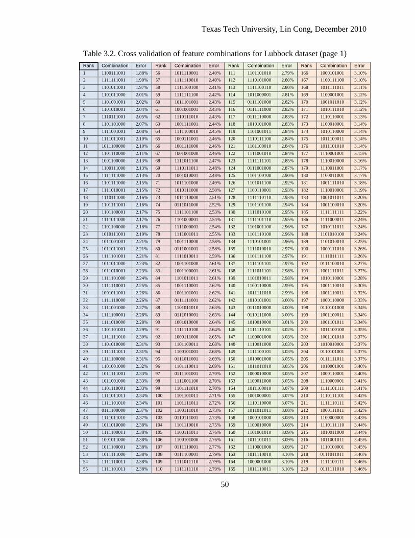
Texas Tech University, Lin Cong, December 2010
50
Table 3.2. Cross validation of feature combinations for Lubbock dataset (page 1) Rank Combination Error Rank Combination Error Rank Combination Error Rank Combination Error 1 1100111001 1.88% 56 1011110001 2.40% 111 1101101010 2.79% 166 1000101001 3.10% 2 1111111001 1.90% 57 1111110010 2.40% 112 1110101000 2.80% 167 1100111100 3.10% 3 1101011001 1.97% 58 1111100100 2.41% 113 1111100110 2.80% 168 1011111011 3.11% 4 1101011000 2.01% 59 1111111100 2.42% 114 1011000001 2.81% 169 1100001001 3.12% 5 1101001001 2.02% 60 1011101001 2.43% 115 0111101000 2.82% 170 1001011010 3.12% 6 1101010001 2.04% 61 1001001001 2.43% 116 0111111000 2.82% 171 1010111010 3.12% 7 1110111001 2.05% 62 1110111010 2.43% 117 0111110000 2.83% 172 1110110001 3.13% 8 1101101000 2.07% 63 1001111001 2.44% 118 1010101000 2.83% 173 1100010001 3.14% 9 1111001001 2.08% 64 1111100010 2.45% 119 1101001011 2.84% 174 1010110000 3.14% 10 1111011001 2.10% 65 1000111001 2.46% 120 1110111100 2.84% 175 1011100011 3.14% 11 1011100000 2.10% 66 1001111000 2.46% 121 1101100010 2.84% 176 1011101010 3.14% 12 1101110000 2.11% 67 1001001000 2.46% 122 1111001010 2.84% 177 1110001001 3.15% 13 1001100000 2.13% 68 1111011100 2.47% 123 1111111101 2.85% 178 1110010000 3.16% 14 1100111000 2.13% 69 1110111011 2.48% 124 0111001000 2.87% 179 1110011001 3.17% 15 1111111000 2.13% 70 1001010001 2.48% 125 1101100100 2.90% 180 1100011001 3.17% 16 1101111000 2.15% 71 1011101000 2.49% 126 1101011100 2.92% 181 1001111010 3.18% 17 1111010001 2.15% 72 1010111000 2.50% 127 1100110001 2.93% 182 1110010001 3.19% 18 1110111000 2.16% 73 1011110000 2.51% 128 1111110110 2.93% 183 1001011011 3.20% 19 1101111001 2.16% 74 0111011000 2.52% 129 1101101100 2.94% 184 1001100010 3.20% 20 1101100001 2.17% 75 1111101100 2.53% 130 1111010100 2.95% 185 1111111111 3.22% 21 1111011000 2.17% 76 1101000001 2.54% 131 1111101110 2.95% 186 1111000011 3.24% 22 1101100000 2.18% 77 1111000001 2.54% 132 1101001100 2.96% 187 1010111011 3.24% 23 1010111001 2.19% 78 1111001011 2.55% 133 1101110100 2.96% 188 1101010100 3.24% 24 1011001001 2.21% 79 1001110000 2.58% 134 1110101001 2.96% 189 1101010010 3.25% 25 1011011001 2.21% 80 0111001001 2.58% 135 1111010010 2.97% 190 1000111010 3.26% 26 1111101001 2.21% 81 1111010011 2.59% 136 1101111100 2.97% 191 1111011111 3.26% 27 1011011000 2.23% 82 1001101000 2.61% 137 1111101101 2.97% 192 0111100010 3.27% 28 1011010001 2.23% 83 1001100001 2.61% 138 1111011101 2.98% 193 1001111011 3.27% 29 1111101000 2.24% 84 1101011011 2.61% 139 1101010011 2.98% 194 1010110001 3.28% 30 1111110001 2.25% 85 1001110001 2.62% 140 1100110000 2.99% 195 1001110010 3.30% 31 1001011001 2.26% 86 1001101001 2.62% 141 1011111010 2.99% 196 1001110011 3.32% 32 1111110000 2.26% 87 0111111001 2.62% 142 1010101001 3.00% 197 1000110000 3.33% 33 1111001000 2.27% 88 1101011010 2.63% 143 0111010000 3.00% 198 0110101000 3.34% 34 1111100001 2.28% 89 0111010001 2.63% 144 0110111000 3.00% 199 1001100011 3.34% 35 1111010000 2.28% 90 1001010000 2.64% 145 1010010000 3.01% 200 1001101011 3.34% 36 1101101001 2.29% 91 1111110100 2.64% 146 1111110101 3.02% 201 1011100100 3.35% 37 1111111010 2.30% 92 1000111000 2.65% 147 1100001000 3.03% 202 1001101010 3.37% 38 1101010000 2.31% 93 1101100011 2.68% 148 1110011000 3.03% 203 1010010001 3.37% 39 1111111011 2.31% 94 1100101001 2.68% 149 1111100101 3.03% 204 0110101001 3.37% 40 1111100000 2.31% 95 0111011001 2.69% 150 1010001000 3.05% 205 0111111011 3.37% 41 1101001000 2.32% 96 1101110011 2.69% 151 1011011010 3.05% 206 1010001001 3.40% 42 1011111001 2.33% 97 0111101001 2.70% 152 1000010000 3.05% 207 1000110001 3.40% 43 1011001000 2.33% 98 1111001100 2.70% 153 1100011000 3.05% 208 1110000001 3.41% 44 1101110001 2.33% 99 1101111010 2.70% 154 1011100010 3.07% 209 1111101111 3.41% 45 1111011011 2.34% 100 1101101011 2.71% 155 1001000001 3.07% 210 1110111101 3.42% 46 1111101010 2.34% 101 1101111011 2.72% 156 1110110000 3.07% 211 1111110111 3.42% 47 0111100000 2.37% 102 1100111010 2.73% 157 1011011011 3.08% 212 1000111011 3.42% 48 1111011010 2.37% 103 0110111001 2.73% 158 1000101000 3.08% 213 1100000001 3.43% 49 1011010000 2.38% 104 1101110010 2.75% 159 1100010000 3.08% 214 1110111110 3.44% 50 1111100011 2.38% 105 1100111011 2.76% 160 1101001010 3.09% 215 1010011000 3.44% 51 1001011000 2.38% 106 1100101000 2.76% 161 1011101011 3.09% 216 1011001011 3.45% 52 1011100001 2.38% 107 0111110001 2.77% 162 1110001000 3.09% 217 1110100001 3.45% 53 1011111000 2.38% 108 0111100001 2.79% 163 1011110010 3.10% 218 0111011011 3.46% 54 1111110011 2.38% 109 1111011110 2.79% 164 1000001000 3.10% 219 1111100111 3.46% 55 1111101011 2.38% 110 1111111110 2.79% 165 1011110011 3.10% 220 0111111010 3.46%

Texas Tech University, Lin Cong, December 2010
51
Table 3.3. Cross validation of feature combinations for New Orleans dataset (page 1) Rank Combination Error Rank Combination Error Rank Combination Error Rank Combination Error 1 1110001001 5.67% 56 1111011100 7.77% 111 0111011000 8.32% 166 1010111000 8.72% 2 1110011001 5.77% 57 1111111011 7.79% 112 1100111000 8.34% 167 0001001001 8.73% 3 1110111000 5.81% 58 0111111001 7.79% 113 0100010001 8.34% 168 1110010110 8.75% 4 1110001000 5.84% 59 0010001001 7.82% 114 1110111110 8.35% 169 1111101110 8.75% 5 1110010001 5.84% 60 1111001100 7.84% 115 1010011001 8.36% 170 1110110110 8.75% 6 1110101000 5.86% 61 0110101001 7.85% 116 0001011001 8.37% 171 1011001001 8.75% 7 1110011000 5.87% 62 1111001011 7.86% 117 0011001001 8.38% 172 1111010110 8.77% 8 1110010000 5.89% 63 1110110100 7.86% 118 0000101001 8.38% 173 0101101001 8.78% 9 1110110000 5.96% 64 1111011010 7.87% 119 0111111000 8.38% 174 0111010011 8.78% 10 1110101001 6.01% 65 1111111100 7.88% 120 1101111001 8.39% 175 0011100001 8.79% 11 1110110001 6.03% 66 1111010011 7.89% 121 1010010001 8.39% 176 1101111000 8.80% 12 1110111001 6.06% 67 0110110001 7.89% 122 0000110001 8.41% 177 0010011000 8.81% 13 1111011000 6.19% 68 0110111000 7.90% 123 0100011001 8.41% 178 0110011011 8.81% 14 1111001000 6.29% 69 0010111001 7.91% 124 0101111001 8.42% 179 1110001110 8.81% 15 1111001001 6.29% 70 1111101010 7.92% 125 1011111001 8.42% 180 1110101101 8.81% 16 1111011001 6.34% 71 1100111001 7.92% 126 0100101001 8.42% 181 0111101011 8.82% 17 1111010000 6.39% 72 0010011001 7.94% 127 1111100011 8.43% 182 1011101001 8.82% 18 1111111000 6.42% 73 1110100100 7.96% 128 1101001001 8.44% 183 0101110001 8.83% 19 1111010001 6.50% 74 1111010100 7.99% 129 0111001000 8.45% 184 1111011101 8.83% 20 1110100001 6.57% 75 0011011001 8.02% 130 1010101001 8.46% 185 0001010001 8.83% 21 1111111001 6.60% 76 0000001001 8.03% 131 0011010001 8.48% 186 0111011100 8.83% 22 1111101000 6.63% 77 0110101000 8.04% 132 1000001001 8.48% 187 0010101000 8.83% 23 1111110001 6.66% 78 0010010001 8.05% 133 1101010001 8.50% 188 1110100000 8.84% 24 1111101001 6.68% 79 0100111001 8.05% 134 1111011110 8.52% 189 0010111011 8.85% 25 1110000001 6.75% 80 0110011000 8.07% 135 1111000100 8.53% 190 0010001100 8.85% 26 1111100001 6.80% 81 1111110010 8.07% 136 0011101001 8.53% 191 0001110001 8.86% 27 1111110000 6.83% 82 0010101001 8.07% 137 0011110001 8.53% 192 1000101001 8.86% 28 1111100000 6.93% 83 1100001001 8.08% 138 0110101011 8.54% 193 1011110001 8.86% 29 1111000001 7.12% 84 1111101011 8.11% 139 0111111011 8.54% 194 0010101100 8.87% 30 1110011010 7.36% 85 0111001001 8.11% 140 1000010001 8.54% 195 1111110110 8.87% 31 1110101010 7.39% 86 1100011001 8.12% 141 1010110001 8.55% 196 0110101100 8.88% 32 0110111001 7.43% 87 1101011001 8.12% 142 1000111001 8.57% 197 0010110000 8.88% 33 1110110010 7.44% 88 0010110001 8.14% 143 1101101001 8.57% 198 1100111011 8.89% 34 1110001100 7.50% 89 0110110000 8.14% 144 0100110001 8.57% 199 1101100001 8.89% 35 1110111011 7.52% 90 1100101001 8.15% 145 1000011001 8.58% 200 0101010001 8.89% 36 1110101011 7.55% 91 1100010001 8.16% 146 0111011011 8.58% 201 0111001100 8.90% 37 1110111100 7.56% 92 1111101100 8.16% 147 0110010000 8.58% 202 1000110001 8.90% 38 0110011001 7.58% 93 1010111001 8.17% 148 0111100001 8.59% 203 0011011000 8.92% 39 1110111010 7.58% 94 0011111001 8.18% 149 1110101110 8.59% 204 0010111100 8.92% 40 0110001001 7.59% 95 1111110011 8.18% 150 1111111110 8.60% 205 0001101001 8.92% 41 1110011011 7.60% 96 1111100100 8.18% 151 1111100010 8.61% 206 1110110101 8.92% 42 1111001010 7.61% 97 1100110001 8.21% 152 1110111101 8.62% 207 1011010001 8.92% 43 1110010100 7.61% 98 0000010001 8.21% 153 1101110001 8.62% 208 0111110011 8.93% 44 1110010010 7.63% 99 0101011001 8.21% 154 0010111000 8.65% 209 0100111000 8.93% 45 1111010010 7.63% 100 1111110100 8.23% 155 1101011000 8.65% 210 0111101000 8.93% 46 1110010011 7.65% 101 1110000100 8.23% 156 0111010000 8.66% 211 1111010101 8.95% 47 1110001010 7.67% 102 0000011001 8.23% 157 1110100010 8.67% 212 1010111100 8.97% 48 1110011100 7.67% 103 0110111011 8.25% 158 0110110011 8.67% 213 0010010100 8.97% 49 1110001011 7.67% 104 0111010001 8.26% 159 0001111001 8.68% 214 0110010011 8.97% 50 1110110011 7.69% 105 0111101001 8.27% 160 0111001011 8.68% 215 1111001101 8.97% 51 1110101100 7.72% 106 1010001001 8.27% 161 0101001001 8.70% 216 0010101011 8.97% 52 0110010001 7.72% 107 0000111001 8.27% 162 0110111100 8.71% 217 1110100011 8.97% 53 1111111010 7.73% 108 0100001001 8.28% 163 1111001110 8.71% 218 0100111011 8.99% 54 0111011001 7.73% 109 1011011001 8.29% 164 1001011001 8.72% 219 1110011101 8.99% 55 1111011011 7.73% 110 0111110001 8.29% 165 1110011110 8.72% 220 1111111101 8.99%

Texas Tech University, Lin Cong, December 2010
52
3.4 Chapter Conclusion The spectral-spatial feature extraction is explained in this chapter. Normalized
correlation and PCA transform are calculated based on the hyperspectral dataset and
provide two independent sources of spectral features. A hierarchical Fourier transform
– co-occurrence matrix method is designed to help extract the macroscopic spatial
patterns from both residential and natural areas. The direction of spatial repetition is
determined by sweeping the Fourier space and searching the angle of maximum
energy. The distribution of co-occurring gray levels in the direction of spatial
repetition is then calculated. Eight different second order texture measures are
calculated from the co-occurrence matrix and compared. K-fold cross validation is
performed for all of the combinations of the features, and a best joint feature vector is
selected for each dataset.
The comparison of classification results between using the purely spectral
feature, using purely spatial feature, and using the joint feature vector is presented in
the next chapter.

Texas Tech University, Lin Cong, December 2010
53
CHAPTER IV
CLASSIFICATION AND RESULTS Both the Bayes classification and K-means clustering methods are used
separately to classify the joint feature vectors into residential and natural classes. The
results of classification and comparisons between the joint solution, the spectral-only
solution and the spatial-only solution are discussed in this chapter.
4.1 Supervised Classification
4.1.1 Bayes Classifier The Bayes classifier is based on Bayes decision theory. The likelihood
function of class iω with respect to the variable x , ( | )ip x ω , is assumed to follow
multivariate Gaussian distribution as shown by equation 4.1, where k stands for the
dimensionality of the variable and iµ and iΣ stand for the mean vector and the
covariance matrix of class iω , which can be estimated from the available training
vectors. As the objective function of each class, the posterior probability, ( | )ip xω ,
can be estimated using Bayes Rule as shown by equation 4.2 [45].
11/2/2
1 1( | ) exp[ ( ) ( )]2(2 )
ti i i ik
i
p x x xω µ µπ
−= − − Σ −Σ
(4.1)
( ) ( | )( | )( )
i ii
P p xP xp x
ω ωω = (4.2)
For two-class application, Bayes classification rule can be stated as
1 2 1
1 2 2
if ( | ) ( | ), is classified asif ( | ) ( | ), is classified as
P x P x xP x P x xω ω ωω ω ω
><
.
4.1.2 Classification Results of Bayes Classifier For the Lubbock dataset, the Bayes classification results that used purely
spectral features, purely spatial features and joint features are displayed in Fig. 4.1 and
Table 4.1. For spectral solution, many small-area misclassifications were found within
residential regions, where manmade structure has low concentration and hence the

Texas Tech University, Lin Cong, December 2010
54
spectral signature is more like that of natural objects; and pixels on and around
country roads were misclassified from the natural class to the residential class. For the
spatial solution, several large-area residential misclassifications were found near Slide
road and the south Loop, where the typical street patterns do not exist. Generally,
according to the error rate, the spectral solution has a better performance for
residential classification while the spatial solution has a better performance for
classifying natural areas.
The joint solution owns the complementary advantages from both the spectral-
only solution and the spatial-only solution: within the residential segmentation, there
is almost no large-area misclassification around the Slide and the south Loop because
of the lack of typical street patterns, and much less small-area misclassification due to
the low concentration of manmade structures; within the natural segmentation,
misclassification around country roads is also lessened.
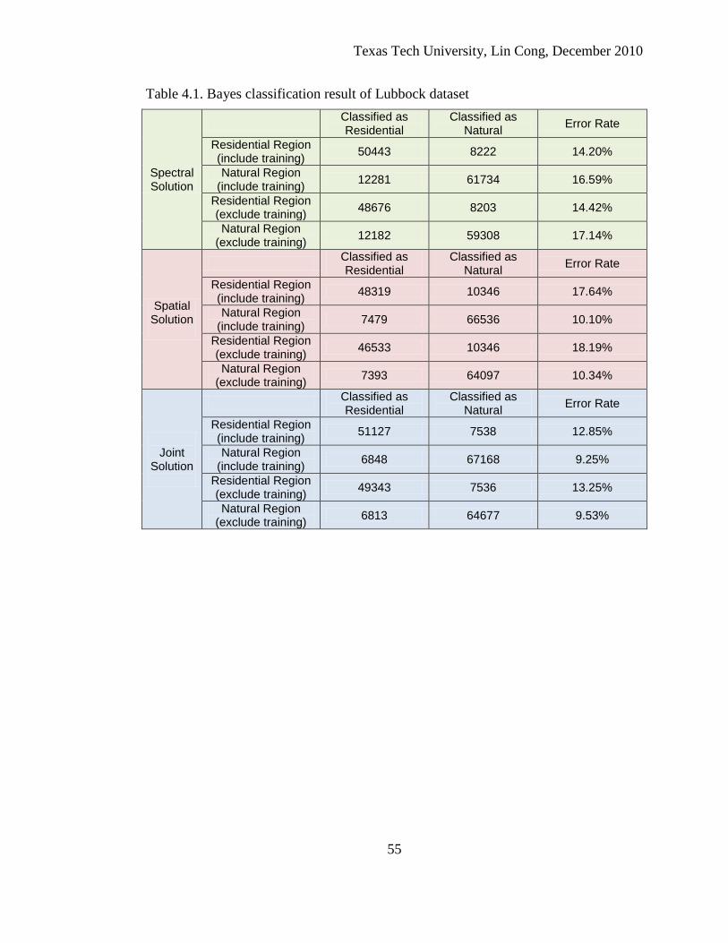
Texas Tech University, Lin Cong, December 2010
55
Table 4.1. Bayes classification result of Lubbock dataset
Spectral Solution
Classified as Residential
Classified as Natural Error Rate
Residential Region (include training) 50443 8222 14.20%
Natural Region (include training) 12281 61734 16.59%
Residential Region (exclude training) 48676 8203 14.42%
Natural Region (exclude training) 12182 59308 17.14%
Spatial Solution
Classified as Residential
Classified as Natural Error Rate
Residential Region (include training) 48319 10346 17.64%
Natural Region (include training) 7479 66536 10.10%
Residential Region (exclude training) 46533 10346 18.19%
Natural Region (exclude training) 7393 64097 10.34%
Joint
Solution
Classified as Residential
Classified as Natural Error Rate
Residential Region (include training) 51127 7538 12.85%
Natural Region (include training) 6848 67168 9.25%
Residential Region (exclude training) 49343 7536 13.25%
Natural Region (exclude training) 6813 64677 9.53%

Texas Tech University, Lin Cong, December 2010
56
(a) (b) (c)
Figure 4.1. Bayes classification of Lubbock dataset (a) Using purely spectral features; (b) Using purely spatial features; (c) Using joint features. Blue: Correct residential region; Green: Correct natural region; Red: Residential region classified as natural; Magenta: Natural region classified as residential.
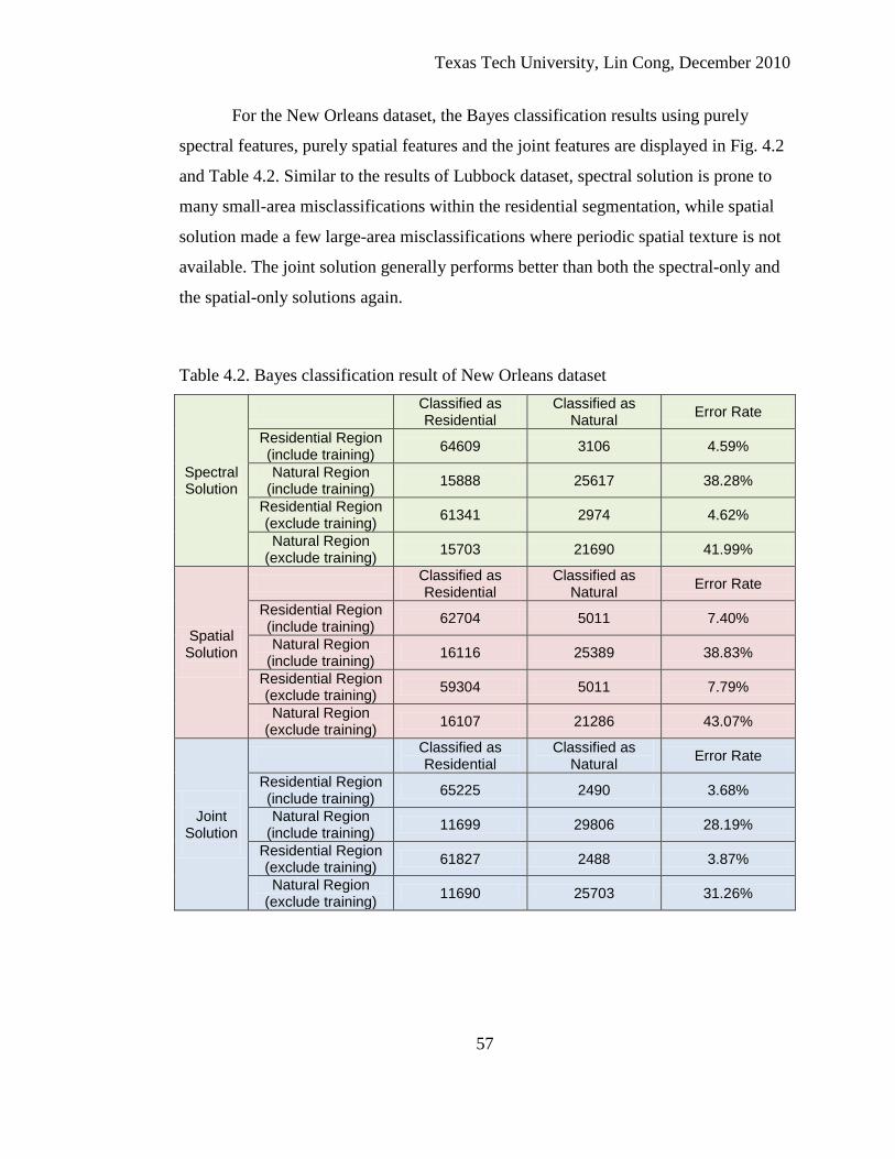
Texas Tech University, Lin Cong, December 2010
57
For the New Orleans dataset, the Bayes classification results using purely
spectral features, purely spatial features and the joint features are displayed in Fig. 4.2
and Table 4.2. Similar to the results of Lubbock dataset, spectral solution is prone to
many small-area misclassifications within the residential segmentation, while spatial
solution made a few large-area misclassifications where periodic spatial texture is not
available. The joint solution generally performs better than both the spectral-only and
the spatial-only solutions again.
Table 4.2. Bayes classification result of New Orleans dataset
Spectral Solution
Classified as Residential
Classified as Natural Error Rate
Residential Region (include training) 64609 3106 4.59%
Natural Region (include training) 15888 25617 38.28%
Residential Region (exclude training) 61341 2974 4.62%
Natural Region (exclude training) 15703 21690 41.99%
Spatial Solution
Classified as Residential
Classified as Natural Error Rate
Residential Region (include training) 62704 5011 7.40%
Natural Region (include training) 16116 25389 38.83%
Residential Region (exclude training) 59304 5011 7.79%
Natural Region (exclude training) 16107 21286 43.07%
Joint
Solution
Classified as Residential
Classified as Natural Error Rate
Residential Region (include training) 65225 2490 3.68%
Natural Region (include training) 11699 29806 28.19%
Residential Region (exclude training) 61827 2488 3.87%
Natural Region (exclude training) 11690 25703 31.26%

Texas Tech University, Lin Cong, December 2010
58
(a) (b) (c)
Figure 4.2. Bayes classification of New Orleans dataset (a) Using purely spectral features; (b) Using purely spatial features; (c) Using joint features. Blue: Correct residential area; Green: Correct natural and river area; Red: Residential area classified as natural or river; Magenta: Natural or river area classified as residential

Texas Tech University, Lin Cong, December 2010
59
4.2 Unsupervised Classification The K-means method is applied to cluster the joint feature vectors. A key to
the success of the K-means method is the initial estimation of the number of clusters
(K). Although it is reasonable to force the number as two (residential and natural
clusters), the complexity of data structures sometimes requires more than two clusters
in order to make each cluster compact. As a result, the “Jump method” of model order
estimation is first applied to estimate the number of clusters, and then K-means is
implemented to both joint feature vectors and purely spectral feature vectors by using
the estimated number as the initial value of K. Finally, several sub-clusters are
combined to form two general clusters, residential and natural region.
4.2.1 Model Order Estimation The “true” number of clusters in the dataset is estimated by “Jump method”
described in [46] - [47]. Below is a brief review of the “Jump method”.
The procedure is based on “distortion”, which is a measure of within-cluster
dispersion. Vector x denotes a p-dimensional variable with a mixture distribution of G
components, each with covariance ∑; let 1 2, ,..., Kc c c be a set of candidate cluster
centers, in which xc denotes the closest one to x . The minimum achievable distortion
associated with fitting K centers to the data is then
1
1
,...,
1 min [( ) ( )]K
tK x xc c
d E x c x cp
−= − Σ − , (4.3)
which is simply the average Mahalanobis distance between each sample and its
nearest center. Note that if the covariance matrix ∑ is the identity matrix, distortion is
simply mean squared error (Euclidian distance). In practice, one generally estimates
Kd using ˆKd , the minimum distortion obtained by applying the K-means clustering
algorithm to the observed data.
Although a natural and simple idea is to find the value of K associated with the
minimum of Kd , the concept is unsuccessful because the distortion function Kd is
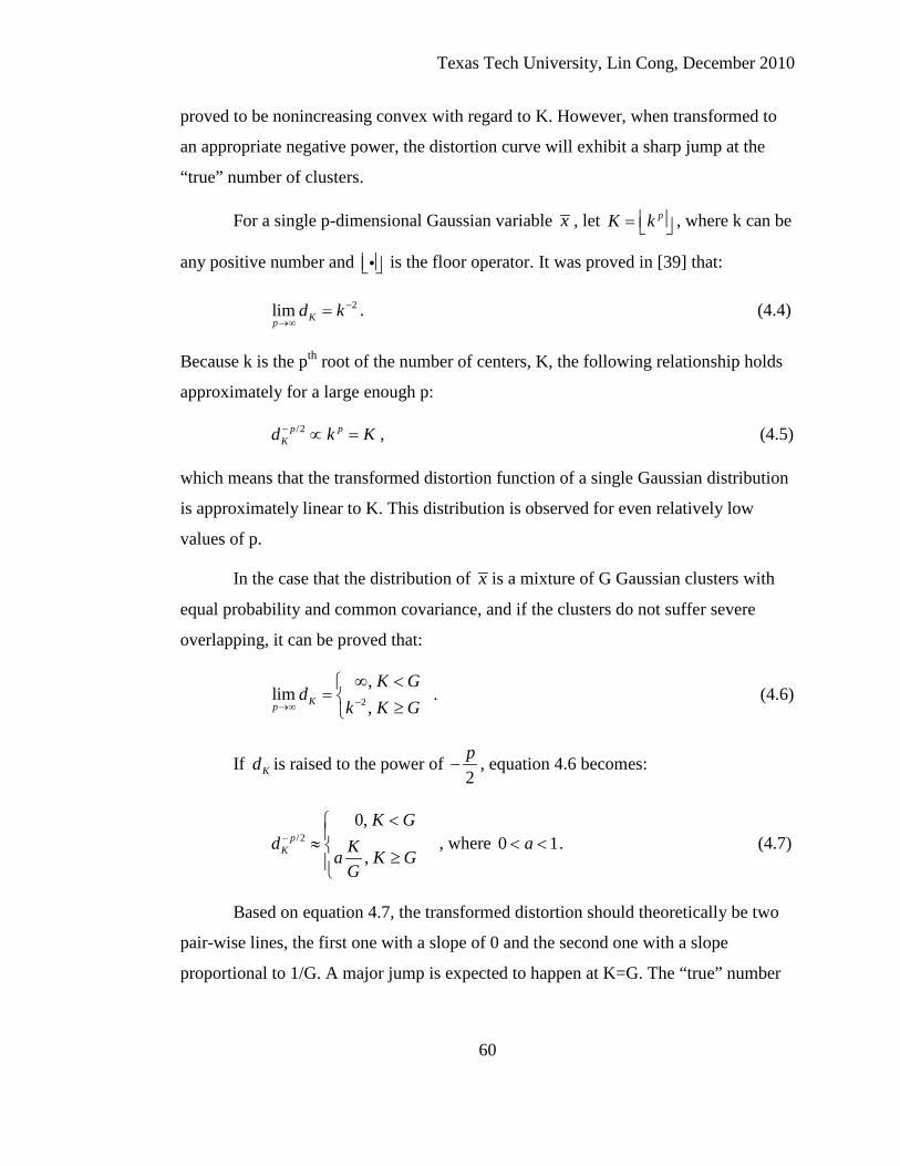
Texas Tech University, Lin Cong, December 2010
60
proved to be nonincreasing convex with regard to K. However, when transformed to
an appropriate negative power, the distortion curve will exhibit a sharp jump at the
“true” number of clusters.
For a single p-dimensional Gaussian variable x , let pK k = , where k can be
any positive number and is the floor operator. It was proved in [39] that:
2lim Kpd k −
→∞= . (4.4)
Because k is the pth root of the number of centers, K, the following relationship holds
approximately for a large enough p:
/2p pKd k K− ∝ = , (4.5)
which means that the transformed distortion function of a single Gaussian distribution
is approximately linear to K. This distribution is observed for even relatively low
values of p.
In the case that the distribution of x is a mixture of G Gaussian clusters with
equal probability and common covariance, and if the clusters do not suffer severe
overlapping, it can be proved that:
2
,lim
,Kp
K Gd
k K G−→∞
∞ <= ≥
. (4.6)
If Kd is raised to the power of 2p
− , equation 4.6 becomes:
/20,
,p
K
K Gd Ka K G
G
−<
≈ ≥
, where 0 1a< < . (4.7)
Based on equation 4.7, the transformed distortion should theoretically be two
pair-wise lines, the first one with a slope of 0 and the second one with a slope
proportional to 1/G. A major jump is expected to happen at K=G. The “true” number

Texas Tech University, Lin Cong, December 2010
61
of clusters can be located by the application of a first order forward difference
operator as in
/2 /21
ˆ ˆarg max[ ]p pK K
KG d d− −
−= − . (4.8)
For more details about the “jump method” and some modifications to improve the
accuracy and computing speed, the reader is referred to [46] – [48].
Texas Tech University, Lin Cong, December 2010
62
(a)
(b)
Figure 4.3. Results of cluster number estimation (a) Purely spectral features for New Orleans data. (b) Joint features for New Orleans data.
1 2 3 4 5 6 7 8 9 1030
40
50
60
70
80
90Estimated Number of Clusters (Kest = 3)
Number of Clusters Tested
JUM
P Va
lue
1 2 3 4 5 6 7 8 9 1015
20
25
30Estimated Number of Clusters (Kest = 4)
Number of Clusters Tested
JUM
P V
alue
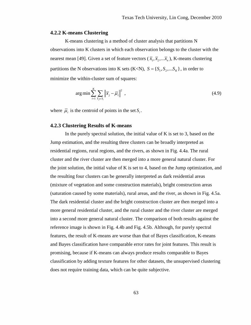
Texas Tech University, Lin Cong, December 2010
63
4.2.2 K-means Clustering K-means clustering is a method of cluster analysis that partitions N
observations into K clusters in which each observation belongs to the cluster with the
nearest mean [49]. Given a set of feature vectors ( 1 2, ,... nx x x ), K-means clustering
partitions the N observations into K sets (K<N), 1 2{ , ,... }KS S S S= , in order to
minimize the within-cluster sum of squares:
2
1arg min
j i
K
j ii x S
x µ= ∈
−∑ ∑ , (4.9)
where iµ is the centroid of points in the set iS .
4.2.3 Clustering Results of K-means In the purely spectral solution, the initial value of K is set to 3, based on the
Jump estimation, and the resulting three clusters can be broadly interpreted as
residential regions, rural regions, and the rivers, as shown in Fig. 4.4a. The rural
cluster and the river cluster are then merged into a more general natural cluster. For
the joint solution, the initial value of K is set to 4, based on the Jump optimization, and
the resulting four clusters can be generally interpreted as dark residential areas
(mixture of vegetation and some construction materials), bright construction areas
(saturation caused by some materials), rural areas, and the river, as shown in Fig. 4.5a.
The dark residential cluster and the bright construction cluster are then merged into a
more general residential cluster, and the rural cluster and the river cluster are merged
into a second more general natural cluster. The comparison of both results against the
reference image is shown in Fig. 4.4b and Fig. 4.5b. Although, for purely spectral
features, the result of K-means are worse than that of Bayes classification, K-means
and Bayes classification have comparable error rates for joint features. This result is
promising, because if K-means can always produce results comparable to Bayes
classification by adding texture features for other datasets, the unsupervised clustering
does not require training data, which can be quite subjective.

Texas Tech University, Lin Cong, December 2010
64
(a) (b)
Figure 4.4. K-means clustering result by using purely spectral features (a) The three clusters found by K-means. Blue: predominantly comprised of residential areas; Green: predominantly comprised of soil areas; Red: predominantly comprised of river. (b) Comparison with the reference after combining the soil and river into a general natural cluster. Blue: correct residential area; Green: correct natural area; Red: residential area classified as natural; Magenta: natural area classified as residential.
Texas Tech University, Lin Cong, December 2010
65
(a) (b)
Figure 4.5. K-means clustering result by using joint solution (a) The four clusters found by K-means. Blue: primarily comprised of residential areas; Green: primarily comprised of soil areas; Red: primarily comprised of saturated residential pixels; Magenta: primarily comprised of river. (b) Comparison with the reference after combining the soil and river into a general natural cluster, and residential and saturated residential pixels into a general residential cluster. Blue: correct residential area; Green: correct natural area; Red: residential area classified as natural; Magenta: natural area classified as residential.

Texas Tech University, Lin Cong, December 2010
66
Table 4.3. K-means clustering result of New Orleans dataset Spectral Solution Residential Area Natural Area
Classified as Residential 52718 8064
Classified as Natural 14997 33441
Error Rate 22.15% 19.43%
Joint Solution Residential Area Natural Area
Classified as Residential 62510 11476
Classified as Natural 5205 30029
Error Rate 7.69% 27.65%
4.3 Chapter Conclusion The comparison of classification results between using joint features, using
purely spectral features and using purely spatial features is presented in this chapter.
Both supervised classification (Bayes classifier) and unsupervised classification (K-
means clustering) are implemented. For Bayes classification, the joint solution
generally has preferable performance for classifying both residential and natural areas
to the purely spectral solutions. The K-means clustering result of the joint solution is
also better than that of purely spectral solutions and comparable to the performance of
supervised classification, which indicates that adding the texture features can improve
the separability between residential and natural data so that training before
classification can be avoided, at least for some datasets.

Texas Tech University, Lin Cong, December 2010
67
CHAPTER V
CONCLUSIONS AND FUTURE WORK In this thesis, a joint spectral-spatial feature extraction method is developed for
residential structure detection from low spatial-resolution Hyperion hyperspectral
datasets.
Chapter I reviewed the current hyperspectral image processing methods,
especially for purely spectral algorithms. In Chapter II, preprocessing including
destriping and atmospheric compensation is introduced. The design of joint features is
presented in Chapter III. Both normalized correlation and the most significant PCA
bands are used as spectral features (Section 3.1). The Hierarchical Fourier transform –
co-occurrence matrix method is developed in Section 3.2. The Fourier transform is
used to detect the direction of the dominant spatially repetitive pattern, and the co-
occurrence matrix is subsequently calculated by using the detected angle. Eight
different texture measures are extracted from the co-occurrence. All the combinations
of the joint features are evaluated by K-fold cross validation, and the best combination
of each dataset (containing PCA1, PCA2, DIS, HOM, SIM and ENT for Lubbock
dataset; containing PCA1, PCA2, spectral correlation, SIM and ENT for New Orleans
dataset) is selected. In Chapter IV, both Bayes classification and K-means clustering
are implemented on Lubbock and New Orleans datasets. The fact that the joint
solution generally performs better than the purely spectral and the purely spatial
solutions proves that merging spectral information with macroscopic texture
information is beneficial for the classification. More testing and verification on
additional datasets are required in the future.
Based on the results in Chapter IV, three conclusions can be received:
(1) Improved accuracy in classification between residential and natural areas was
achieved by using both spectral and macroscopic spatial information.
(2) Improved accuracy in unsupervised clustering can be also achieved by adding
spatial features.

Texas Tech University, Lin Cong, December 2010
68
The segmentations of residential and natural areas may have, but are not
limited to, the following two applications:
(1) Comparing the segmentations of residential areas before and after a hurricane in
the same position may be an effective method to analyze the disaster effect on the
urban region, as the street structures may be destroyed after a severe hurricane.
(2) The segmentations of residential and natural areas can be used for model choice in
spectral unmixing. For pixels within the segmentation of residential areas, models
containing construction materials will have higher likelihood to use for unmixing; for
pixels within the natural segmentation, models not containing construction materials
will have higher likelihood of use. The sub-pixel classification may be able to interpret
the hurricane effect on the city.
Texas Tech University, Lin Cong, December 2010
69
BIBLIOGRAPHY [1] American Association for Wind Engineering, "Wind Engineering Research and
Outreach Plan to Reduce Losses Due to Wind Hazards," Fort Collins, CO (Published in collaboration with ASCE), 2004
[2] Louisiana Department of Health and Hospitals (2006, Aug.), Reports of Missing and Deceased, Deceased Reports. [Online]. http://www.dhh.louisiana.gov/offices/page.asp?ID=192&Detail=5248
[3] AP Photo/U.S. Coast Guard, Petty Officer 2nd Class Kyle Niemi. (2005, Aug.) Wikipedia. [Online]. http://en.wikipedia.org/wiki/Hurricane_Katrina#cite_note-louisiana1-0
[4] Wikipedia. [Online]. http://en.wikipedia.org/wiki/File:Hurricane_katrina_damage_gulfport_mississippi.jpg
[5] S. Watt, "Using Remote sensing Technology," Damage Assessment Report, 2004. [6] Nirupama and S. P. Simonovic, "Role of Remote Sensing in Disaster Management,"
Institute for Catastrophic Loss Reduction, the University of Western Ontario, 2002. [7] M. Gevonder, K. Chetty, and H. Bulcock, "A review of hyperspectral remote sensing
and its application in vegetation and water resource studies," Water SA, vol. 33, no. 2, pp. 145-152, Apr. 2007.
[8] P. Shippert, "Introduction to Hyperspectral Image Analysis", Remote Sensing of Earth via Satellite, no. 3, 2003.
[9] F. A. Kruse, et al., "The Spectral Image Processing System (SIPS) - Interactive Visualization and Analysis of Imaging Spectrometer Data," Remote Sens. Environ, no. 44, pp. 145-163, 1993.
[10] SIPS User's Guide, The Spectral Image Processing System, v.1.1, Center for the Study of Earth from Space (CSES), University of Colorado at Boulder, CO, 1992.
[11] R. N. Clark, A. J. Gallagher, and G. A. Swayze, "Material absorption band depth mapping of imaging spectrometer data using the complete band shape least-squares algorithm simultaneously fit to multiple spectral features from multiple materials," in Proceedings of the Third Airborne Visible/Infrared Imaging Spectrometer (AVIRIS) Workshop, JPL Publication, vol. 54, 1990, pp. 176-186.
[12] R. N. Clark, G. A. Swayze, A. Gallagher, N. Gorelick, and F. A. Kruse, "Mapping with imaging spectrometer data using the complete band shape least-squares algorithm simultaneously fit to multiple spectral features from multiple materials," in Proceedings of Third Airborne Visible/Infrared Imaging Spectrometer (AVIRIS) workshop, JPL Publication, vol. 28, 1991, pp. 2-3.
[13] R. N. Clark, G. A. Swayze, and A. Gallagher, "Mapping the mineralogy and lithology of Canyonlands, Utah with imaging spectrometer data and the multiple spectral feature mapping algorithm," in Summaries of the Third Annual JPL Airborne Geoscience Workshop, JPL Publication, vol. I, 1992, pp. 11-13.
[14] R. N. Clark and G. A. Swayze, "Mapping minerals, amorphous materials, environmental materials, vegetation, water, ice, and snow, and other materials: The USGS Tricorder Algorithm," in Summaries of the Fifth Annual JPL Airborne Earth Science Workshop, JPL Publication, vol. I, 1995, pp. 39-40.
Texas Tech University, Lin Cong, December 2010
70
[15] ENVI Tutorial: Selected Hyperspectral Mapping Methods, ITT Visual Information Solution, Boulder, CO.
[16] J. W. Boardman and F. A. Kruse, "Automated spectral analysis: A geological example using AVIRIS data, northern Grapevine Mountains, Nevada," in Proceedings of Tenth Thematic Conference, Geologic Remote Sensing, vol. I, San Antonio, Texas, 1994, pp. 407-418.
[17] M. K. Ridd, "Exploring a V-I-S (vegetation - impervious surface - soil) model for urban ecosystem analysis through remote sensing: comparative anatomy for cities," International Journal of Remote Sensing, no. 16, pp. 2165-2185, 1995.
[18] T. Kardi, "Remote sensing of urban areas: linear spectral unmixing of Landsat Thematic Mapper images acquired over Tartu (Estonia)," in Proc. Estonian Acad. Sci. Biol. Ecol., 2007.
[19] R. L. Powell, D. A. Roberts, P. E. Dennison, and L. L. Hess, "Sub-pixel mapping of urban land cover using multiple endmember spectral mixture analysis: Manaus, Brazil," Remote Sensing of Environment, no. 106, pp. 253-267, 2007.
[20] J. Franke, D. A. Roberts, K. Halligan, and G. Menz, "Hierarchical Multiple Endmember Spectral Mixture Analysis (MESMA) of hyperspectral imagery for urban environments," Remote Sensing of Environment, no. 113, pp. 1712-1723, 2009.
[21] S. W. Myint and G. S. Okin, "Modeling Land-Cover Types Using Multiple Endmember Spectral Mixture Analysis in Desert City," GEODA center for Geospatial Analysis and computation, Arizona State University Working Paper Number 2010-06, 2010.
[22] C. Small, "High resolution spectral mixture analysis of urban reflectance," Remote Sensing of Environment, no. 88, pp. 170-186, 2003.
[23] L. Cong, B. Nutter, and D. Liang, "Grid Pattern Based Residential Area Detection from Hyperion Data," in Proceedings of IEEE Southwest Symposium on Image Analysis and Interpretation, Austin, TX, 2010, pp. 105-108.
[24] L. M. Bruce, H. Tamhankar, A. Mathur, and R. King, "Multiresolutional texture analysis of multispectral imagery for automated ground cover classification," in Geoscience and Remote Sensing Symposium, IEEE International, vol. I, 2002, pp. 312-314.
[25] M. Shi and G. Healey, "Using multiband correlation models for the invariant recognition of 3-D hyperspectral textures," IEEE Transactions on Geoscience and Remote Sensing, vol. 43, no. 5, pp. 1201-1209, 2005.
[26] M. Shi and G. Healey, "Hyperspectral texture recognition using a multiscale opponent representation," IEEE Transactions on Geoscience and Remote Sensing, vol. 41, no. 5, pp. 1090-1095, 2003.
[27] K. Lee, S. H. Jeon, and B. Doo-Kwon, "Urban Feature Characterization using High-Resolution Satellite Imagery: Texture Analysis Approach," in Map Asia Conference, 2004.

Texas Tech University, Lin Cong, December 2010
71
[28] Y. C. Huang, P. Li, L. Zhang, and Y. Zhong, "Urban Land Cover Mapping by Spatial-Spectral Feature Analysis of High Resolution Hyperspectral Data with Decision Directed Acyclic Graph SVM," in Urban Remote Sensing Event, IEEE conference, 2009, pp. 1-7.
[29] C. Song, F. Yang, and P. Li, "Rotation Invariant Texture Measured by Local Binary Pattern for Remote Sensing Image Classification," in Second International Workshop on Education Technology and Computer Science, 2010.
[30] G. Rellier, X. Descombes, J. Zerubia, and F. Falzon, "A Gauss-Markov Model for Hyperspectral Texture Analysis of Urban Areas," in Proceedings of IEEE International Conference on Pattern Recognition, vol. 1, 2002, pp. 692-695.
[31] R. Beck, "EO-1 User Guide, Version 2.3," Satellite Systems Branch, USGS Earth Resources Observation Systems Data Center (EDC), 2003.
[32] ENVI Tutorial: FLAASH Module Users' Guide, ITT Visual Information Solutions, Boulder, CO.
[33] Wikipedia. [Online]. http://upload.wikimedia.org/wikipedia/commons/4/4c/Solar_Spectrum.png
[34] Introduction to Hyperspectral Imaging, MicroImages Inc, Lincoln, NE, 2010. [Online]. http://www.microimages.com/documentation/Tutorials/hyprspec.pdf
[35] Y. J. Kaufman, et al., "The Modis 2.1 - m Channel - Correlation with Visible Reflectance for Use in Remote Sensing of Aerosol," IEEE Transactions on Geoscience and Remote Sensing, vol. 35, no. 5, 1997.
[36] E. F. Vermote, et al., "Atmospheric correction of visible to middle-infrared EOS-MODIS data over land surfaces: Background, operational algorithm and validation," Journal of Geophysical Research, vol. 102, no. 14, pp. 17131-17141, 1997.
[37] S. M. Adler-Golden, et al., "Atmospheric Correction for Short-wave Spectral Imagery Based on MODTRAN4," SPIE Proceeding, Imaging Spectrometry V, vol. 3753, 1999.
[38] A. Berk, et al., "MODTRAN Cloud and Multiple Scattering Upgrades with Application to AVIRIS," Remote Sensing Environment, vol. 65, pp. 367-375, 1998.
[39] T. Cooley, et al., "FLAASH, a MODTRAN4-based Atmospheric correction Algorithm, Its Application and Validation," in IEEE International Symposium on Geoscience and Remote Sensing, vol. 3, 2002, pp. 1414-1418.
[40] R. N. Clark, et al. (2007, Sep.) USGS Digital Spectral Library splib06a. [Online]. http://speclab.cr.usgs.gov/spectral.lib06/
[41] wikipedia. [Online]. http://en.wikipedia.org/wiki/Principle_components_analysis [42] R. O. Duda, P. E. Hart, and D. G. Stork, Pattern Classification, 2nd ed. Wiley. [43] R. M. Haralick, K. Shanmugam, and I. Dinstein, "Textural Features for Image
Classification," IEEE Transactions on Systems, Man, and Cybernetics, vol. 3, no. 6, 1973.
[44] M. Hall-Beyer. (2007, Feb.) The GLCM Tutorial Home Page (v 2.10). [Online]. http://www.fp.ucalgary.ca/mhallbey/tutorial.htm
[45] S. Theodoridis and K. Koutroumbas, Pattern Recognition, 2nd ed. Academic Press, 2003.

Texas Tech University, Lin Cong, December 2010
72
[46] C. A. Suger and G. M. James, "Finding the Number of Clusters in a Dataset: An
Information-Theoretic Approach," Journal of the American Statistical Association, vol. 98, no. 463, Sep. 2003.
[47] E. Corona, B. Nutter, and S. Mitra, "Non-parametric Estimation of Mixture Model Order," in 2008 IEEE Southwest Symposium on Image Analysis and Interpretation, Santa Fe, 2008.
[48] E. Corona, B. Nutter, and S. Mitra, "Optimized Data-Driven Order Selection Method for Gaussian Mixtures on," in 2010 IEEE Southwest Symposium on Image Analysis and Interpretation (SSIAI), Austin, TX, 2010.
[49] Wikipedia. [Online]. http://en.wikipedia.org/wiki/K-means_clustering

Texas Tech University, Lin Cong, December 2010
73
APPENDIX The full tables of the cross validation of feature combinations are listed in this
appendix.
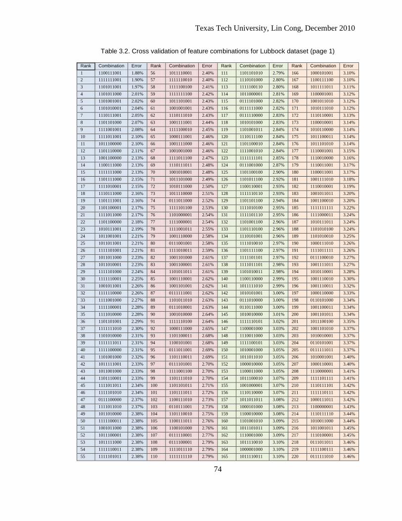
Texas Tech University, Lin Cong, December 2010
74
Table 3.2. Cross validation of feature combinations for Lubbock dataset (page 1)
Rank Combination Error Rank Combination Error Rank Combination Error Rank Combination Error 1 1100111001 1.88% 56 1011110001 2.40% 111 1101101010 2.79% 166 1000101001 3.10% 2 1111111001 1.90% 57 1111110010 2.40% 112 1110101000 2.80% 167 1100111100 3.10% 3 1101011001 1.97% 58 1111100100 2.41% 113 1111100110 2.80% 168 1011111011 3.11% 4 1101011000 2.01% 59 1111111100 2.42% 114 1011000001 2.81% 169 1100001001 3.12% 5 1101001001 2.02% 60 1011101001 2.43% 115 0111101000 2.82% 170 1001011010 3.12% 6 1101010001 2.04% 61 1001001001 2.43% 116 0111111000 2.82% 171 1010111010 3.12% 7 1110111001 2.05% 62 1110111010 2.43% 117 0111110000 2.83% 172 1110110001 3.13% 8 1101101000 2.07% 63 1001111001 2.44% 118 1010101000 2.83% 173 1100010001 3.14% 9 1111001001 2.08% 64 1111100010 2.45% 119 1101001011 2.84% 174 1010110000 3.14% 10 1111011001 2.10% 65 1000111001 2.46% 120 1110111100 2.84% 175 1011100011 3.14% 11 1011100000 2.10% 66 1001111000 2.46% 121 1101100010 2.84% 176 1011101010 3.14% 12 1101110000 2.11% 67 1001001000 2.46% 122 1111001010 2.84% 177 1110001001 3.15% 13 1001100000 2.13% 68 1111011100 2.47% 123 1111111101 2.85% 178 1110010000 3.16% 14 1100111000 2.13% 69 1110111011 2.48% 124 0111001000 2.87% 179 1110011001 3.17% 15 1111111000 2.13% 70 1001010001 2.48% 125 1101100100 2.90% 180 1100011001 3.17% 16 1101111000 2.15% 71 1011101000 2.49% 126 1101011100 2.92% 181 1001111010 3.18% 17 1111010001 2.15% 72 1010111000 2.50% 127 1100110001 2.93% 182 1110010001 3.19% 18 1110111000 2.16% 73 1011110000 2.51% 128 1111110110 2.93% 183 1001011011 3.20% 19 1101111001 2.16% 74 0111011000 2.52% 129 1101101100 2.94% 184 1001100010 3.20% 20 1101100001 2.17% 75 1111101100 2.53% 130 1111010100 2.95% 185 1111111111 3.22% 21 1111011000 2.17% 76 1101000001 2.54% 131 1111101110 2.95% 186 1111000011 3.24% 22 1101100000 2.18% 77 1111000001 2.54% 132 1101001100 2.96% 187 1010111011 3.24% 23 1010111001 2.19% 78 1111001011 2.55% 133 1101110100 2.96% 188 1101010100 3.24% 24 1011001001 2.21% 79 1001110000 2.58% 134 1110101001 2.96% 189 1101010010 3.25% 25 1011011001 2.21% 80 0111001001 2.58% 135 1111010010 2.97% 190 1000111010 3.26% 26 1111101001 2.21% 81 1111010011 2.59% 136 1101111100 2.97% 191 1111011111 3.26% 27 1011011000 2.23% 82 1001101000 2.61% 137 1111101101 2.97% 192 0111100010 3.27% 28 1011010001 2.23% 83 1001100001 2.61% 138 1111011101 2.98% 193 1001111011 3.27% 29 1111101000 2.24% 84 1101011011 2.61% 139 1101010011 2.98% 194 1010110001 3.28% 30 1111110001 2.25% 85 1001110001 2.62% 140 1100110000 2.99% 195 1001110010 3.30% 31 1001011001 2.26% 86 1001101001 2.62% 141 1011111010 2.99% 196 1001110011 3.32% 32 1111110000 2.26% 87 0111111001 2.62% 142 1010101001 3.00% 197 1000110000 3.33% 33 1111001000 2.27% 88 1101011010 2.63% 143 0111010000 3.00% 198 0110101000 3.34% 34 1111100001 2.28% 89 0111010001 2.63% 144 0110111000 3.00% 199 1001100011 3.34% 35 1111010000 2.28% 90 1001010000 2.64% 145 1010010000 3.01% 200 1001101011 3.34% 36 1101101001 2.29% 91 1111110100 2.64% 146 1111110101 3.02% 201 1011100100 3.35% 37 1111111010 2.30% 92 1000111000 2.65% 147 1100001000 3.03% 202 1001101010 3.37% 38 1101010000 2.31% 93 1101100011 2.68% 148 1110011000 3.03% 203 1010010001 3.37% 39 1111111011 2.31% 94 1100101001 2.68% 149 1111100101 3.03% 204 0110101001 3.37% 40 1111100000 2.31% 95 0111011001 2.69% 150 1010001000 3.05% 205 0111111011 3.37% 41 1101001000 2.32% 96 1101110011 2.69% 151 1011011010 3.05% 206 1010001001 3.40% 42 1011111001 2.33% 97 0111101001 2.70% 152 1000010000 3.05% 207 1000110001 3.40% 43 1011001000 2.33% 98 1111001100 2.70% 153 1100011000 3.05% 208 1110000001 3.41% 44 1101110001 2.33% 99 1101111010 2.70% 154 1011100010 3.07% 209 1111101111 3.41% 45 1111011011 2.34% 100 1101101011 2.71% 155 1001000001 3.07% 210 1110111101 3.42% 46 1111101010 2.34% 101 1101111011 2.72% 156 1110110000 3.07% 211 1111110111 3.42% 47 0111100000 2.37% 102 1100111010 2.73% 157 1011011011 3.08% 212 1000111011 3.42% 48 1111011010 2.37% 103 0110111001 2.73% 158 1000101000 3.08% 213 1100000001 3.43% 49 1011010000 2.38% 104 1101110010 2.75% 159 1100010000 3.08% 214 1110111110 3.44% 50 1111100011 2.38% 105 1100111011 2.76% 160 1101001010 3.09% 215 1010011000 3.44% 51 1001011000 2.38% 106 1100101000 2.76% 161 1011101011 3.09% 216 1011001011 3.45% 52 1011100001 2.38% 107 0111110001 2.77% 162 1110001000 3.09% 217 1110100001 3.45% 53 1011111000 2.38% 108 0111100001 2.79% 163 1011110010 3.10% 218 0111011011 3.46% 54 1111110011 2.38% 109 1111011110 2.79% 164 1000001000 3.10% 219 1111100111 3.46% 55 1111101011 2.38% 110 1111111110 2.79% 165 1011110011 3.10% 220 0111111010 3.46%

Texas Tech University, Lin Cong, December 2010
75
Table 3.2. (cont.) Cross validation of feature combinations for Lubbock dataset (page 2)
Rank Combination Error Rank Combination Error Rank Combination Error Rank Combination Error 221 0111101011 3.46% 276 1110110100 3.74% 331 1100111101 4.16% 386 0111011110 4.48% 222 1101100110 3.47% 277 1011110100 3.74% 332 1100110011 4.17% 387 1110110101 4.48% 223 1000011000 3.47% 278 1000111100 3.75% 333 1110111111 4.17% 388 0111111101 4.48% 224 1111000100 3.47% 279 1001010011 3.76% 334 0101111001 4.17% 389 0111010010 4.48% 225 1111000010 3.47% 280 1110001100 3.77% 335 1001000010 4.18% 390 1001011110 4.48% 226 1101000011 3.47% 281 0111010011 3.77% 336 0101011000 4.19% 391 1110101110 4.48% 227 0110110000 3.48% 282 1110001011 3.78% 337 0111001010 4.19% 392 1100000011 4.49% 228 1101011110 3.48% 283 1001111100 3.78% 338 1111001111 4.19% 393 1110001101 4.49% 229 1000001001 3.49% 284 1011010010 3.78% 339 1100010011 4.20% 394 0101100000 4.50% 230 1010011001 3.50% 285 1011101100 3.78% 340 1100001011 4.20% 395 1010101011 4.51% 231 1000010001 3.50% 286 1110110010 3.80% 341 1001010100 4.21% 396 1000101010 4.52% 232 1111001110 3.50% 287 1110010010 3.80% 342 1011111101 4.22% 397 1001011101 4.53% 233 1111001101 3.51% 288 1111010101 3.80% 343 1110011101 4.22% 398 0101001001 4.53% 234 1101111110 3.51% 289 1011001100 3.81% 344 1000100001 4.23% 399 1101101111 4.53% 235 1100100001 3.52% 290 0111101010 3.82% 345 1100100000 4.23% 400 1101110111 4.55% 236 0111100011 3.52% 291 0110111100 3.82% 346 1100111110 4.23% 401 1110110110 4.55% 237 1011011100 3.52% 292 1110100010 3.82% 347 1110011110 4.23% 402 1100000010 4.56% 238 0111110011 3.52% 293 1110010100 3.83% 348 1101001110 4.24% 403 1100100100 4.57% 239 1101000010 3.53% 294 0111100100 3.83% 349 0100111001 4.27% 404 1010100000 4.57% 240 1011001010 3.54% 295 0111101100 3.83% 350 1100101100 4.28% 405 1010010010 4.59% 241 0110001000 3.55% 296 1111010110 3.84% 351 1011011110 4.29% 406 0110101011 4.60% 242 0110111011 3.55% 297 1110010011 3.84% 352 1101111111 4.30% 407 0111101110 4.60% 243 1000011001 3.56% 298 0111011100 3.85% 353 1100011100 4.30% 408 1101000000 4.61% 244 1110011011 3.57% 299 1100011010 3.86% 354 1111000101 4.31% 409 1010110010 4.61% 245 1001001011 3.58% 300 0111110010 3.86% 355 1011011101 4.31% 410 0111110110 4.62% 246 1110011010 3.58% 301 1001010010 3.86% 356 1100001100 4.31% 411 1110010110 4.62% 247 1011111100 3.58% 302 1001001100 3.88% 357 1010101010 4.31% 412 1011101110 4.63% 248 0110010000 3.58% 303 0111001100 3.88% 358 0101101001 4.31% 413 0100111000 4.63% 249 1101111101 3.59% 304 0110011001 3.89% 359 1110101101 4.33% 414 0111000011 4.63% 250 1101101110 3.59% 305 0111110100 3.89% 360 1001111110 4.33% 415 0101111000 4.64% 251 1001100100 3.60% 306 0110010001 3.90% 361 1011000011 4.33% 416 1110000110 4.64% 252 0111001011 3.60% 307 1100101010 3.93% 362 0101110001 4.33% 417 1000101011 4.65% 253 1010000001 3.61% 308 1110100100 3.96% 363 1100100011 4.34% 418 1010011011 4.65% 254 0111111100 3.61% 309 1001101100 3.96% 364 1001111101 4.34% 419 1100000100 4.65% 255 0110110001 3.64% 310 1110100011 3.96% 365 0111111110 4.35% 420 1000011011 4.65% 256 1101100101 3.64% 311 0110111010 3.98% 366 0110000001 4.35% 421 1101100111 4.66% 257 1101110110 3.65% 312 1100101011 3.98% 367 1101011111 4.35% 422 1000100000 4.67% 258 1110101011 3.66% 313 0110001001 3.99% 368 1111010111 4.37% 423 1010001011 4.68% 259 1101101101 3.66% 314 1100100010 3.99% 369 1101001101 4.37% 424 0111011101 4.69% 260 1001011100 3.66% 315 1111000110 4.01% 370 1010011010 4.38% 425 1110100101 4.69% 261 1101110101 3.67% 316 1001110100 4.01% 371 1100110100 4.38% 426 1011101101 4.72% 262 1101011101 3.67% 317 1100001010 4.01% 372 1001000011 4.39% 427 1011110110 4.72% 263 1110101100 3.67% 318 1100011011 4.03% 373 1010001010 4.39% 428 1110010101 4.73% 264 1010111100 3.68% 319 1011010100 4.04% 374 0101100001 4.41% 429 1011100101 4.73% 265 0111011010 3.68% 320 1110000011 4.05% 375 1100010100 4.41% 430 1010110011 4.73% 266 1001001010 3.68% 321 1110000010 4.08% 376 0110100001 4.41% 431 0101110000 4.74% 267 1101000100 3.69% 322 1011111110 4.08% 377 1001000100 4.42% 432 0101101000 4.74% 268 1110011100 3.69% 323 1110000100 4.11% 378 1110100110 4.43% 433 1101010110 4.74% 269 1110101010 3.70% 324 1110100000 4.12% 379 1010100010 4.44% 434 1011110101 4.77% 270 1000000001 3.70% 325 1010100001 4.12% 380 1111000000 4.45% 435 1000110010 4.77% 271 1011010011 3.70% 326 0111010100 4.12% 381 0111100110 4.45% 436 1101010101 4.78% 272 1110001010 3.71% 327 1100110010 4.14% 382 1110001110 4.45% 437 1000010010 4.78% 273 1110110011 3.73% 328 1011000010 4.14% 383 1000011010 4.45% 438 0110001011 4.80% 274 0111000001 3.73% 329 1100010010 4.15% 384 1011100110 4.45% 439 1011000100 4.80% 275 0110011000 3.73% 330 0101011001 4.16% 385 1000001010 4.46% 440 1010111101 4.81%

Texas Tech University, Lin Cong, December 2010
76
Table 3.2. (cont.) Cross validation of feature combinations for Lubbock dataset (page 3)
Rank Combination Error Rank Combination Error Rank Combination Error Rank Combination Error 441 1001100110 4.84% 496 0100101000 5.21% 551 1100010110 5.67% 606 0011001000 6.20% 442 0101010001 4.84% 497 1000100100 5.21% 552 0010111001 5.68% 607 0000111000 6.21% 443 1110011111 4.84% 498 1110010111 5.21% 553 1100110110 5.71% 608 0100010000 6.22% 444 0110001010 4.85% 499 0111101111 5.22% 554 1110000000 5.72% 609 1010101101 6.23% 445 1000001011 4.86% 500 0111001101 5.22% 555 1110000111 5.72% 610 1000111111 6.24% 446 0110101010 4.86% 501 1010110100 5.23% 556 0101011011 5.72% 611 0100001000 6.24% 447 0111101101 4.87% 502 0110100000 5.24% 557 1100000110 5.74% 612 0101110100 6.28% 448 1000100010 4.87% 503 1100011101 5.24% 558 0100001001 5.76% 613 0110001101 6.29% 449 0110011011 4.87% 504 1010000011 5.25% 559 0100111011 5.77% 614 0110000010 6.30% 450 0110010011 4.88% 505 0111110111 5.26% 560 1100010101 5.78% 615 0110011101 6.30% 451 1010010011 4.88% 506 0110100011 5.26% 561 1101010111 5.80% 616 0001001000 6.31% 452 0111000100 4.89% 507 1110100111 5.26% 562 0101100010 5.82% 617 0110011110 6.31% 453 0110110011 4.89% 508 1011011111 5.29% 563 0011111001 5.82% 618 0110101101 6.32% 454 0110011010 4.90% 509 1000001100 5.29% 564 0110111111 5.83% 619 0001100000 6.33% 455 1000110011 4.90% 510 1011001101 5.30% 565 0101100011 5.85% 620 1010011101 6.33% 456 0111001110 4.90% 511 1010100100 5.30% 566 0100010001 5.85% 621 0110000110 6.33% 457 1111000111 4.91% 512 1011001110 5.30% 567 0001111000 5.85% 622 0001110000 6.35% 458 0111110101 4.92% 513 1010010100 5.31% 568 0101111100 5.86% 623 0100111100 6.35% 459 1000111101 4.95% 514 1001111111 5.31% 569 0010111000 5.88% 624 0101101010 6.35% 460 1001101110 4.96% 515 1011000000 5.31% 570 0101111010 5.88% 625 0111010111 6.35% 461 0101001000 4.96% 516 0100101001 5.32% 571 0101101011 5.89% 626 0011101001 6.39% 462 1101000110 4.96% 517 0111010110 5.32% 572 0100011001 5.90% 627 0110010110 6.39% 463 0110111110 4.97% 518 0110110100 5.34% 573 0100110001 5.90% 628 0110110110 6.39% 464 0110100010 4.98% 519 0111100111 5.34% 574 0001111001 5.90% 629 0010101000 6.41% 465 1110101111 4.98% 520 1000000100 5.35% 575 1011010110 5.91% 630 0011001001 6.42% 466 1010111110 4.99% 521 1000110100 5.37% 576 0101110011 5.94% 631 0101011010 6.43% 467 1010101100 5.00% 522 1101001111 5.37% 577 0100110000 5.95% 632 0110010101 6.44% 468 1010100011 5.00% 523 0110001100 5.42% 578 0111001111 5.96% 633 1010000000 6.45% 469 0111111111 5.01% 524 1100110101 5.44% 579 1011101111 5.96% 634 1000011101 6.45% 470 1110110111 5.02% 525 0110000011 5.44% 580 1001000000 5.97% 635 0111000101 6.45% 471 1001100101 5.03% 526 1100001101 5.45% 581 1100100101 5.97% 636 1010001101 6.46% 472 1001110110 5.03% 527 0101111011 5.45% 582 0100011000 5.99% 637 1100101111 6.46% 473 0110111101 5.04% 528 0011011000 5.47% 583 1011010101 5.99% 638 0001101001 6.47% 474 1000010011 5.05% 529 1100011110 5.48% 584 1011110111 6.00% 639 0101110010 6.47% 475 1001101101 5.05% 530 0011011001 5.48% 585 0011100000 6.01% 640 1000101101 6.49% 476 0111100101 5.05% 531 0001011000 5.48% 586 0101100100 6.01% 641 1000011110 6.52% 477 1001110101 5.06% 532 1100101110 5.49% 587 1100000000 6.02% 642 1100001111 6.53% 478 1110001111 5.06% 533 0110011100 5.50% 588 1011100111 6.04% 643 1010011110 6.53% 479 1000000010 5.08% 534 1000000011 5.50% 589 1010111111 6.04% 644 0110100110 6.54% 480 0111000010 5.09% 535 0110100100 5.51% 590 0011101000 6.05% 645 0001001001 6.54% 481 1000100011 5.09% 536 1000010100 5.52% 591 1001010110 6.10% 646 0110110101 6.55% 482 0110010010 5.09% 537 1100001110 5.52% 592 0000111001 6.10% 647 0101001100 6.56% 483 0111011111 5.10% 538 1010000100 5.53% 593 0111000000 6.10% 648 0101010011 6.59% 484 1010001100 5.11% 539 0001011001 5.53% 594 1100011111 6.12% 649 1010101110 6.59% 485 1010000010 5.11% 540 1001001101 5.54% 595 1001110111 6.13% 650 1010001110 6.61% 486 1010011100 5.11% 541 0111000110 5.54% 596 0110001110 6.13% 651 0011001000 6.62% 487 0110110010 5.14% 542 0110010100 5.56% 597 0101011100 6.15% 652 0000111000 6.63% 488 1000111110 5.15% 543 1001011111 5.56% 598 0101101100 6.15% 653 0100010000 6.64% 489 1011111111 5.15% 544 1101000101 5.57% 599 1001101111 6.15% 654 1010101101 6.64% 490 1000011100 5.16% 545 0011111000 5.57% 600 0101001011 6.16% 655 1000111111 6.64% 491 1000101100 5.18% 546 0101010000 5.58% 601 0110101110 6.17% 656 0100001000 6.69% 492 0110101100 5.18% 547 1001001110 5.59% 602 0001101000 6.17% 657 0101110100 6.70% 493 1100101101 5.18% 548 0110000100 5.62% 603 1001010101 6.18% 658 0110001101 6.70% 494 1110000101 5.19% 549 1100100110 5.64% 604 1001100111 6.18% 659 0110000010 6.71% 495 1100111111 5.21% 550 0111010101 5.64% 605 0011110000 6.19% 660 0110011101 6.77%

Texas Tech University, Lin Cong, December 2010
77
Table 3.2. (cont.) Cross validation of feature combinations for Lubbock dataset (page 4)
Rank Combination Error Rank Combination Error Rank Combination Error Rank Combination Error 661 1010110101 6.80% 716 1010011111 7.41% 771 1000101111 8.12% 826 0011001010 8.98% 662 1100110111 6.81% 717 0101101111 7.42% 772 0010010001 8.12% 827 0011111101 9.09% 663 0100111010 6.82% 718 0110100111 7.42% 773 0101010110 8.14% 828 0100000100 9.10% 664 1100000101 6.83% 719 0100001011 7.43% 774 0101001101 8.14% 829 0001111101 9.13% 665 1001000110 6.83% 720 0101110111 7.44% 775 0001101011 8.15% 830 0011111111 9.18% 666 1000001101 6.84% 721 0101101101 7.47% 776 0001100010 8.16% 831 0100101110 9.19% 667 1011000110 6.86% 722 0100101011 7.48% 777 0100101100 8.16% 832 0001101110 9.22% 668 0001110001 6.88% 723 1000011111 7.49% 778 0100000001 8.17% 833 0010101011 9.22% 669 0011110001 6.89% 724 0101110101 7.49% 779 1000001111 8.18% 834 0100100100 9.23% 670 1101000111 6.89% 725 0101100101 7.50% 780 0000111010 8.18% 835 0001111111 9.25% 671 1011001111 6.90% 726 1001010111 7.51% 781 0011110011 8.20% 836 0001001010 9.27% 672 0101111111 6.91% 727 0000110000 7.52% 782 0011101010 8.20% 837 0001001100 9.29% 673 1000101110 6.92% 728 0010111011 7.52% 783 0000010001 8.22% 838 0011001100 9.30% 674 0001100001 6.92% 729 1010000110 7.53% 784 1010110111 8.23% 839 0100100000 9.30% 675 1000001110 6.93% 730 0100111110 7.53% 785 1010010111 8.24% 840 0100101101 9.32% 676 1000100110 6.94% 731 0000011000 7.57% 786 0010111100 8.25% 841 0011101110 9.32% 677 0101111110 6.95% 732 1000000110 7.57% 787 0001110011 8.28% 842 0100100011 9.35% 678 0000101000 6.95% 733 0100100001 7.58% 788 0100010100 8.30% 843 1010000111 9.38% 679 1100010111 6.97% 734 1001000101 7.59% 789 0100010010 8.31% 844 0100100010 9.40% 680 1010100110 6.97% 735 0101010010 7.60% 790 0001001011 8.32% 845 0101000110 9.42% 681 1010010110 6.98% 736 0011011010 7.63% 791 0000111100 8.32% 846 1000000111 9.45% 682 1100100111 6.99% 737 0011111100 7.65% 792 0100011010 8.33% 847 0011010010 9.49% 683 0101010100 7.01% 738 0001111100 7.67% 793 1000110111 8.33% 848 0011011110 9.49% 684 1010110110 7.04% 739 1011000101 7.68% 794 0001100011 8.35% 849 0010001011 9.49% 685 0011010001 7.04% 740 0010010000 7.68% 795 0100011100 8.38% 850 0001011110 9.55% 686 0011100001 7.04% 741 0101001110 7.69% 796 0100110010 8.40% 851 0100000011 9.55% 687 1010010101 7.04% 742 1100000111 7.70% 797 0011100011 8.40% 852 0001110110 9.57% 688 0110011111 7.07% 743 0100111101 7.71% 798 0101000011 8.41% 853 0000001011 9.59% 689 1000110101 7.08% 744 0011011011 7.74% 799 0100110100 8.42% 854 0100110110 9.59% 690 0110101111 7.09% 745 0000001000 7.74% 800 1000010111 8.45% 855 0000101011 9.60% 691 0111000111 7.09% 746 0000001001 7.75% 801 0101001111 8.46% 856 0011110110 9.61% 692 0011010000 7.10% 747 0000010000 7.76% 802 0101000100 8.48% 857 0100001101 9.62% 693 0101011110 7.11% 748 0100010011 7.81% 803 0011110010 8.48% 858 0110000000 9.66% 694 0001010001 7.12% 749 0000011001 7.82% 804 1001000111 8.52% 859 0010111110 9.66% 695 0101111101 7.12% 750 0001011010 7.82% 805 0001101010 8.53% 860 0010010011 9.66% 696 1000110110 7.17% 751 1000000000 7.84% 806 0011010011 8.53% 861 0100001110 9.69% 697 0101011111 7.17% 752 0110000111 7.85% 807 0011011100 8.54% 862 0011011111 9.71% 698 1001001111 7.18% 753 0010111010 7.86% 808 0001011100 8.56% 863 0001100110 9.77% 699 0101011101 7.20% 754 0010001001 7.87% 809 0101010101 8.58% 864 0100101111 9.78% 700 0110100101 7.20% 755 1010001111 7.88% 810 1011000111 8.62% 865 0001010100 9.78% 701 0101000001 7.21% 756 0000111011 7.89% 811 0001110010 8.63% 866 0100110101 9.79% 702 0110110111 7.22% 757 1010101111 7.89% 812 1000100111 8.65% 867 0100011101 9.79% 703 0110001111 7.23% 758 0100001010 7.91% 813 1010000101 8.65% 868 0000111110 9.79% 704 0011111010 7.25% 759 0100110011 7.94% 814 0001101100 8.69% 869 0100011111 9.79% 705 0011111011 7.26% 760 0001011011 7.97% 815 1010100111 8.70% 870 0011101111 9.80% 706 1000010110 7.30% 761 0000110001 7.99% 816 0001100100 8.70% 871 0100010101 9.80% 707 0010101001 7.31% 762 0100111111 7.99% 817 1000000101 8.73% 872 0100010110 9.81% 708 1000010101 7.31% 763 0100011011 7.99% 818 0011111110 8.73% 873 0011010100 9.81% 709 0101100110 7.32% 764 0011100010 8.00% 819 0001111110 8.74% 874 0001011111 9.82% 710 0001010000 7.33% 765 0010011001 8.00% 820 0001010011 8.75% 875 0011011101 9.82% 711 0101001010 7.33% 766 0010110001 8.04% 821 0011101100 8.77% 876 0010110011 9.83% 712 0000101001 7.35% 767 0100101010 8.04% 822 0101010111 8.85% 877 0001010010 9.84% 713 0110000101 7.37% 768 0011101011 8.08% 823 0011100100 8.90% 878 0001101111 9.84% 714 0001111011 7.37% 769 0011001011 8.10% 824 0001110100 8.91% 879 0100001111 9.86% 715 0101101110 7.40% 770 0100001100 8.10% 825 0011110100 8.91% 880 0100011110 9.87%

Texas Tech University, Lin Cong, December 2010
78
Table 3.2. (cont.) Cross validation of feature combinations for Lubbock dataset (page 5)
Rank Combination Error Rank Combination Error Rank Combination Error Rank Combination Error 881 0010001010 9.87% 917 0001010110 10.5% 953 0010000001 11.5% 989 0000100100 12.1% 882 0010011011 9.87% 918 0000010010 10.6% 954 0001000100 11.5% 990 0010100100 12.2% 883 0011100110 9.88% 919 0100100111 10.6% 955 0010101111 11.7% 991 0000011101 12.2% 884 0011110111 9.88% 920 0100100101 10.6% 956 0010110110 11.7% 992 0000100011 12.2% 885 0000001010 9.90% 921 0011000001 10.6% 957 0010101101 11.7% 993 0010110101 12.2% 886 0000010011 9.92% 922 0011100101 10.6% 958 0000001111 11.8% 994 0000100010 12.2% 887 0010101010 9.93% 923 0001001101 10.6% 959 0011000110 11.8% 995 0000000100 12.2% 888 0001011101 9.94% 924 0011001111 10.6% 960 0000110110 11.8% 996 0010011101 12.2% 889 0001001110 9.94% 925 0001001111 10.6% 961 0010001111 11.8% 997 0011000101 12.3% 890 0001110111 9.95% 926 0001100101 10.7% 962 0010001110 11.8% 998 0010100010 12.3% 891 0101000111 9.96% 927 0000101100 10.7% 963 0000101111 11.8% 999 0001000101 12.3% 892 0100010111 9.99% 928 0100000111 10.7% 964 0000010110 11.8% 1000 0000110101 12.4% 893 0010011010 10.0% 929 0000001100 10.7% 965 0010010110 11.8% 1001 0010100111 12.4% 894 0100110111 10.0% 930 0100000101 10.7% 966 0000001110 11.8% 1002 0010100000 12.4% 895 0011001110 10.0% 931 0010101100 10.8% 967 0010011111 11.8% 1003 0000100111 12.5% 896 0010111101 10.0% 932 0010001100 10.8% 968 0000101101 11.9% 1004 0000100000 12.5% 897 0011101101 10.1% 933 0011010111 10.9% 969 0000011111 11.9% 1005 0010000110 12.7% 898 0001101101 10.1% 934 0001000001 10.9% 970 0010110111 11.9% 1006 0010000111 12.7% 899 0000111101 10.1% 935 0000110010 10.9% 971 0001000110 11.9% 1007 0000000111 12.7% 900 0101000101 10.1% 936 0000010100 10.9% 972 0011000111 11.9% 1008 0010100110 12.8% 901 0000110011 10.1% 937 0000100001 10.9% 973 0010010111 11.9% 1009 0000000110 12.8% 902 0000101010 10.1% 938 0101000010 11.0% 974 0000000001 11.9% 1010 0000100110 12.9% 903 0011100111 10.1% 939 0001010111 11.0% 975 0000110111 11.9% 1011 0010100101 13.0% 904 0000011011 10.1% 940 0000011100 11.0% 976 0010001101 11.9% 1012 0010000101 13.0% 905 0001100111 10.2% 941 0010010100 11.1% 977 0000010111 11.9% 1013 0000100101 13.1% 906 0011110101 10.2% 942 0010100001 11.1% 978 0010011110 12.0% 1014 0000000101 13.2% 907 0001110101 10.2% 943 0011010101 11.1% 979 0001000111 12.0% 1015 0011000010 13.2% 908 0010111111 10.3% 944 0010011100 11.1% 980 0010000011 12.0% 1016 0101000000 13.7% 909 0000111111 10.3% 945 0011000011 11.1% 981 0000001101 12.0% 1017 0001000010 14.7% 910 0100100110 10.4% 946 0001010101 11.1% 982 0100000010 12.0% 1018 0010000010 15.3% 911 0100000110 10.4% 947 0010110100 11.1% 983 0010000100 12.0% 1019 0000000010 15.8% 912 0000011010 10.4% 948 0000110100 11.1% 984 0010010101 12.1% 1020 0011000000 16.1% 913 0010010010 10.4% 949 0011000100 11.4% 985 0010100011 12.1% 1021 0001000000 19.4% 914 0010110010 10.4% 950 0001000011 11.4% 986 0000011110 12.1% 1022 0010000000 24.4% 915 0011010110 10.5% 951 0010101110 11.4% 987 0000000011 12.1% 1023 0100000000 27.2% 916 0011001101 10.5% 952 0000101110 11.4% 988 0000010101 12.1%

Texas Tech University, Lin Cong, December 2010
79
Table 3.3. Cross validation of feature combinations for New Orleans dataset (page 1)
Rank Combination Error Rank Combination Error Rank Combination Error Rank Combination Error 1 1110001001 5.67% 56 1111011100 7.77% 111 0111011000 8.32% 166 1010111000 8.72% 2 1110011001 5.77% 57 1111111011 7.79% 112 1100111000 8.34% 167 0001001001 8.73% 3 1110111000 5.81% 58 0111111001 7.79% 113 0100010001 8.34% 168 1110010110 8.75% 4 1110001000 5.84% 59 0010001001 7.82% 114 1110111110 8.35% 169 1111101110 8.75% 5 1110010001 5.84% 60 1111001100 7.84% 115 1010011001 8.36% 170 1110110110 8.75% 6 1110101000 5.86% 61 0110101001 7.85% 116 0001011001 8.37% 171 1011001001 8.75% 7 1110011000 5.87% 62 1111001011 7.86% 117 0011001001 8.38% 172 1111010110 8.77% 8 1110010000 5.89% 63 1110110100 7.86% 118 0000101001 8.38% 173 0101101001 8.78% 9 1110110000 5.96% 64 1111011010 7.87% 119 0111111000 8.38% 174 0111010011 8.78% 10 1110101001 6.01% 65 1111111100 7.88% 120 1101111001 8.39% 175 0011100001 8.79% 11 1110110001 6.03% 66 1111010011 7.89% 121 1010010001 8.39% 176 1101111000 8.80% 12 1110111001 6.06% 67 0110110001 7.89% 122 0000110001 8.41% 177 0010011000 8.81% 13 1111011000 6.19% 68 0110111000 7.90% 123 0100011001 8.41% 178 0110011011 8.81% 14 1111001000 6.29% 69 0010111001 7.91% 124 0101111001 8.42% 179 1110001110 8.81% 15 1111001001 6.29% 70 1111101010 7.92% 125 1011111001 8.42% 180 1110101101 8.81% 16 1111011001 6.34% 71 1100111001 7.92% 126 0100101001 8.42% 181 0111101011 8.82% 17 1111010000 6.39% 72 0010011001 7.94% 127 1111100011 8.43% 182 1011101001 8.82% 18 1111111000 6.42% 73 1110100100 7.96% 128 1101001001 8.44% 183 0101110001 8.83% 19 1111010001 6.50% 74 1111010100 7.99% 129 0111001000 8.45% 184 1111011101 8.83% 20 1110100001 6.57% 75 0011011001 8.02% 130 1010101001 8.46% 185 0001010001 8.83% 21 1111111001 6.60% 76 0000001001 8.03% 131 0011010001 8.48% 186 0111011100 8.83% 22 1111101000 6.63% 77 0110101000 8.04% 132 1000001001 8.48% 187 0010101000 8.83% 23 1111110001 6.66% 78 0010010001 8.05% 133 1101010001 8.50% 188 1110100000 8.84% 24 1111101001 6.68% 79 0100111001 8.05% 134 1111011110 8.52% 189 0010111011 8.85% 25 1110000001 6.75% 80 0110011000 8.07% 135 1111000100 8.53% 190 0010001100 8.85% 26 1111100001 6.80% 81 1111110010 8.07% 136 0011101001 8.53% 191 0001110001 8.86% 27 1111110000 6.83% 82 0010101001 8.07% 137 0011110001 8.53% 192 1000101001 8.86% 28 1111100000 6.93% 83 1100001001 8.08% 138 0110101011 8.54% 193 1011110001 8.86% 29 1111000001 7.12% 84 1111101011 8.11% 139 0111111011 8.54% 194 0010101100 8.87% 30 1110011010 7.36% 85 0111001001 8.11% 140 1000010001 8.54% 195 1111110110 8.87% 31 1110101010 7.39% 86 1100011001 8.12% 141 1010110001 8.55% 196 0110101100 8.88% 32 0110111001 7.43% 87 1101011001 8.12% 142 1000111001 8.57% 197 0010110000 8.88% 33 1110110010 7.44% 88 0010110001 8.14% 143 1101101001 8.57% 198 1100111011 8.89% 34 1110001100 7.50% 89 0110110000 8.14% 144 0100110001 8.57% 199 1101100001 8.89% 35 1110111011 7.52% 90 1100101001 8.15% 145 1000011001 8.58% 200 0101010001 8.89% 36 1110101011 7.55% 91 1100010001 8.16% 146 0111011011 8.58% 201 0111001100 8.90% 37 1110111100 7.56% 92 1111101100 8.16% 147 0110010000 8.58% 202 1000110001 8.90% 38 0110011001 7.58% 93 1010111001 8.17% 148 0111100001 8.59% 203 0011011000 8.92% 39 1110111010 7.58% 94 0011111001 8.18% 149 1110101110 8.59% 204 0010111100 8.92% 40 0110001001 7.59% 95 1111110011 8.18% 150 1111111110 8.60% 205 0001101001 8.92% 41 1110011011 7.60% 96 1111100100 8.18% 151 1111100010 8.61% 206 1110110101 8.92% 42 1111001010 7.61% 97 1100110001 8.21% 152 1110111101 8.62% 207 1011010001 8.92% 43 1110010100 7.61% 98 0000010001 8.21% 153 1101110001 8.62% 208 0111110011 8.93% 44 1110010010 7.63% 99 0101011001 8.21% 154 0010111000 8.65% 209 0100111000 8.93% 45 1111010010 7.63% 100 1111110100 8.23% 155 1101011000 8.65% 210 0111101000 8.93% 46 1110010011 7.65% 101 1110000100 8.23% 156 0111010000 8.66% 211 1111010101 8.95% 47 1110001010 7.67% 102 0000011001 8.23% 157 1110100010 8.67% 212 1010111100 8.97% 48 1110011100 7.67% 103 0110111011 8.25% 158 0110110011 8.67% 213 0010010100 8.97% 49 1110001011 7.67% 104 0111010001 8.26% 159 0001111001 8.68% 214 0110010011 8.97% 50 1110110011 7.69% 105 0111101001 8.27% 160 0111001011 8.68% 215 1111001101 8.97% 51 1110101100 7.72% 106 1010001001 8.27% 161 0101001001 8.70% 216 0010101011 8.97% 52 0110010001 7.72% 107 0000111001 8.27% 162 0110111100 8.71% 217 1110100011 8.97% 53 1111111010 7.73% 108 0100001001 8.28% 163 1111001110 8.71% 218 0100111011 8.99% 54 0111011001 7.73% 109 1011011001 8.29% 164 1001011001 8.72% 219 1110011101 8.99% 55 1111011011 7.73% 110 0111110001 8.29% 165 1110011110 8.72% 220 1111111101 8.99%
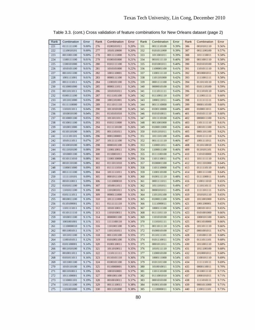
Texas Tech University, Lin Cong, December 2010
80
Table 3.3. (cont.) Cross validation of feature combinations for New Orleans dataset (page 2)
Rank Combination Error Rank Combination Error Rank Combination Error Rank Combination Error 221 0111111100 9.00% 276 0100101011 9.20% 331 0011110100 9.39% 386 0010101110 9.56% 222 1110010101 9.00% 277 1010110000 9.20% 332 0101011000 9.39% 387 0011100100 9.57% 223 0011001100 9.00% 278 0011111000 9.21% 333 1011001011 9.39% 388 1011110011 9.58% 224 1100111100 9.01% 279 0100101000 9.21% 334 0010111110 9.40% 389 0011001110 9.58% 225 1100101000 9.01% 280 0101111100 9.21% 335 0101001011 9.40% 390 0101010100 9.58% 226 1010101100 9.01% 281 1010101000 9.22% 336 1100001100 9.41% 391 1101011110 9.58% 227 0011011100 9.01% 282 1001110001 9.23% 337 1100111110 9.41% 392 0010001011 9.58% 228 1001111001 9.01% 283 0000111100 9.23% 338 1101101000 9.42% 393 1111001111 9.58% 229 0011111011 9.02% 284 1100101100 9.23% 339 0001111100 9.42% 394 0110110110 9.59% 230 0110001000 9.02% 285 0000111011 9.24% 340 0000010100 9.42% 395 0101110100 9.59% 231 0011011011 9.03% 286 1010101011 9.24% 341 1111011111 9.43% 396 0111010110 9.60% 232 0100111100 9.03% 287 0111101100 9.24% 342 0111001110 9.43% 397 1110011111 9.60% 233 1011011000 9.03% 288 1001101001 9.24% 343 1000111011 9.44% 398 1111111111 9.60% 234 0111110000 9.03% 289 0111011110 9.24% 344 0011110000 9.44% 399 0000110100 9.60% 235 1101011011 9.04% 290 1011010100 9.24% 345 0100110000 9.44% 400 0100011011 9.60% 236 1010010100 9.04% 291 0110101010 9.25% 346 0101010011 9.44% 401 0101011110 9.60% 237 0110001100 9.05% 292 1011011011 9.25% 347 1011110100 9.45% 402 0000011100 9.61% 238 0110011100 9.05% 293 0101111000 9.26% 348 0011001000 9.45% 403 1101111110 9.61% 239 1010011000 9.06% 294 0111110100 9.26% 349 0100011000 9.45% 404 1001011100 9.61% 240 0110110100 9.06% 295 0011101011 9.26% 350 0101101011 9.45% 405 0001101100 9.62% 241 1111101101 9.06% 296 0001100001 9.27% 351 1011101100 9.45% 406 0101111110 9.62% 242 1010111011 9.07% 297 1011111100 9.27% 352 0011111110 9.46% 407 1001111011 9.63% 243 0110010100 9.08% 298 0000101100 9.28% 353 1100011011 9.46% 408 0110110010 9.63% 244 0111010100 9.08% 299 1100110011 9.29% 354 1100011100 9.46% 409 0110101101 9.63% 245 1010001100 9.08% 300 0110001011 9.29% 355 0111100100 9.47% 410 1101010000 9.63% 246 0110111010 9.08% 301 1100110000 9.29% 356 1101110011 9.47% 411 1011111110 9.63% 247 0010110100 9.08% 302 0111011010 9.30% 357 0100001100 9.47% 412 1011101000 9.64% 248 1100011000 9.09% 303 0111111010 9.30% 358 1101110000 9.47% 413 0111110110 9.64% 249 0011111100 9.09% 304 1011111011 9.30% 359 1100110100 9.47% 414 1001111100 9.64% 250 1111110101 9.09% 305 0001011100 9.30% 360 0100111110 9.48% 415 0111100011 9.64% 251 0010110011 9.09% 306 1111000010 9.31% 361 0001111011 9.49% 416 1100111010 9.65% 252 0101011100 9.09% 307 1010011011 9.32% 362 1011101011 9.49% 417 1110110111 9.65% 253 1101011100 9.10% 308 1101001011 9.32% 363 0000101011 9.49% 418 1111101111 9.65% 254 0101111011 9.10% 309 0000111000 9.33% 364 1101101100 9.50% 419 1010101110 9.65% 255 0010011100 9.10% 310 1011111000 9.33% 365 0100011100 9.50% 420 1011001000 9.65% 256 0110100001 9.10% 311 0111111110 9.33% 366 1111000011 9.50% 421 1001100001 9.65% 257 1101111011 9.10% 312 1010110011 9.33% 367 1000111100 9.50% 422 1001011011 9.65% 258 0110111110 9.10% 313 1101010011 9.33% 368 0111101110 9.51% 423 0101001000 9.66% 259 1010011100 9.11% 314 0000001100 9.34% 369 1101010100 9.51% 424 1000101100 9.66% 260 1001001001 9.11% 315 1111100110 9.34% 370 1110101111 9.51% 425 0011010000 9.66% 261 1110000010 9.11% 316 1101001100 9.34% 371 0011011110 9.52% 426 1011011110 9.66% 262 0011001011 9.11% 317 1101101011 9.35% 372 0100010100 9.52% 427 0001001011 9.67% 263 1011011100 9.12% 318 0011101100 9.35% 373 0110111101 9.52% 428 1101001110 9.68% 264 1100101011 9.12% 319 0101001100 9.35% 374 0101110011 9.53% 429 0111011101 9.68% 265 0101100001 9.14% 320 0100110011 9.35% 375 0001011011 9.53% 430 1011001110 9.68% 266 0011010100 9.15% 321 1011010011 9.35% 376 1010111110 9.53% 431 1011100100 9.68% 267 0010011011 9.16% 322 1110111111 9.35% 377 1100010100 9.54% 432 1010001011 9.68% 268 0101011011 9.16% 323 0110101110 9.36% 378 1000111000 9.54% 433 1100101110 9.69% 269 1011001100 9.17% 324 0100101100 9.36% 379 0101101100 9.55% 434 1111110111 9.69% 270 1010110100 9.19% 325 0110000001 9.36% 380 1010010011 9.55% 435 0000110011 9.70% 271 0011010011 9.19% 326 1001010001 9.37% 381 1101110100 9.55% 436 0110011110 9.71% 272 1011100001 9.19% 327 0001001100 9.37% 382 0111001010 9.56% 437 1000101011 9.71% 273 1110001101 9.19% 328 0010010011 9.37% 383 0001010100 9.56% 438 1111010111 9.71% 274 1101111100 9.19% 329 0011110011 9.38% 384 0100110100 9.56% 439 0001011000 9.71% 275 1101001000 9.19% 330 0011101000 9.38% 385 1110000011 9.56% 440 1100111101 9.73%
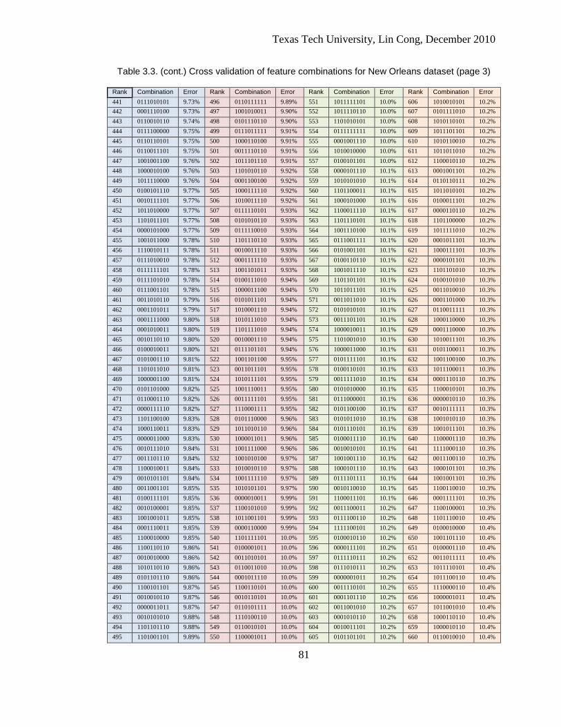
Texas Tech University, Lin Cong, December 2010
81
Table 3.3. (cont.) Cross validation of feature combinations for New Orleans dataset (page 3)
Rank Combination Error Rank Combination Error Rank Combination Error Rank Combination Error 441 0111010101 9.73% 496 0110111111 9.89% 551 1011111101 10.0% 606 1010010101 10.2% 442 0001110100 9.73% 497 1001010011 9.90% 552 1011110110 10.0% 607 0101111010 10.2% 443 0110010110 9.74% 498 0101110110 9.90% 553 1101010101 10.0% 608 1010110101 10.2% 444 0111100000 9.75% 499 0111011111 9.91% 554 0111111111 10.0% 609 1011101101 10.2% 445 0110110101 9.75% 500 1000110100 9.91% 555 0001001110 10.0% 610 1010110010 10.2% 446 0110011101 9.75% 501 0011110110 9.91% 556 1010010000 10.0% 611 1011011010 10.2% 447 1001001100 9.76% 502 1011101110 9.91% 557 0100101101 10.0% 612 1100010110 10.2% 448 1000010100 9.76% 503 1101010110 9.92% 558 0000101110 10.1% 613 0001001101 10.2% 449 1011110000 9.76% 504 0001100100 9.92% 559 1010101010 10.1% 614 0110110111 10.2% 450 0100101110 9.77% 505 1000111110 9.92% 560 1101100011 10.1% 615 1011010101 10.2% 451 0010111101 9.77% 506 1010011110 9.92% 561 1000101000 10.1% 616 0100011101 10.2% 452 1011010000 9.77% 507 0111110101 9.93% 562 1100011110 10.1% 617 0000110110 10.2% 453 1101011101 9.77% 508 0101010110 9.93% 563 1101110101 10.1% 618 1101100000 10.2% 454 0000101000 9.77% 509 0111110010 9.93% 564 1001110100 10.1% 619 1011111010 10.2% 455 1001011000 9.78% 510 1101110110 9.93% 565 0111001111 10.1% 620 0001011101 10.3% 456 1110010111 9.78% 511 0010011110 9.93% 566 0101001101 10.1% 621 1000111101 10.3% 457 0111010010 9.78% 512 0001111110 9.93% 567 0100110110 10.1% 622 0000101101 10.3% 458 0111111101 9.78% 513 1001101011 9.93% 568 1001011110 10.1% 623 1101101010 10.3% 459 0111101010 9.78% 514 0100111010 9.94% 569 1101101101 10.1% 624 0100101010 10.3% 460 0111001101 9.78% 515 1000011100 9.94% 570 1011011101 10.1% 625 0011010010 10.3% 461 0011010110 9.79% 516 0101011101 9.94% 571 0011011010 10.1% 626 0001101000 10.3% 462 0001101011 9.79% 517 1010001110 9.94% 572 0101010101 10.1% 627 0110011111 10.3% 463 0001111000 9.80% 518 1010111010 9.94% 573 0011101101 10.1% 628 1000110000 10.3% 464 0001010011 9.80% 519 1101111010 9.94% 574 1000010011 10.1% 629 0001110000 10.3% 465 0010110110 9.80% 520 0010001110 9.94% 575 1101001010 10.1% 630 1010011101 10.3% 466 0100010011 9.80% 521 0111101101 9.94% 576 1000011000 10.1% 631 0101100011 10.3% 467 0101001110 9.81% 522 1001101100 9.95% 577 0101111101 10.1% 632 1001100100 10.3% 468 1101011010 9.81% 523 0011011101 9.95% 578 0100110101 10.1% 633 1011100011 10.3% 469 1000001100 9.81% 524 1010111101 9.95% 579 0011111010 10.1% 634 0001110110 10.3% 470 0101101000 9.82% 525 1001110011 9.95% 580 0101010000 10.1% 635 1100010101 10.3% 471 0110001110 9.82% 526 0011111101 9.95% 581 0111000001 10.1% 636 0000010110 10.3% 472 0000111110 9.82% 527 1110001111 9.95% 582 0101100100 10.1% 637 0010111111 10.3% 473 1101100100 9.83% 528 0101110000 9.96% 583 0101011010 10.1% 638 1001010110 10.3% 474 1000110011 9.83% 529 1011010110 9.96% 584 0101110101 10.1% 639 1001011101 10.3% 475 0000011000 9.83% 530 1000011011 9.96% 585 0100011110 10.1% 640 1100001110 10.3% 476 0010111010 9.84% 531 1001111000 9.96% 586 0010010101 10.1% 641 1111000110 10.3% 477 0011101110 9.84% 532 1001010100 9.97% 587 1001001110 10.1% 642 0011100110 10.3% 478 1100010011 9.84% 533 1010010110 9.97% 588 1000101110 10.1% 643 1000101101 10.3% 479 0010101101 9.84% 534 1001111110 9.97% 589 0111101111 10.1% 644 1001001101 10.3% 480 0011001101 9.85% 535 1010101101 9.97% 590 0010110010 10.1% 645 1100110010 10.3% 481 0100111101 9.85% 536 0000010011 9.99% 591 1100011101 10.1% 646 0001111101 10.3% 482 0010100001 9.85% 537 1100101010 9.99% 592 0011100011 10.2% 647 1100100001 10.3% 483 1001001011 9.85% 538 1011001101 9.99% 593 0111100110 10.2% 648 1101110010 10.4% 484 0001110011 9.85% 539 0000110000 9.99% 594 1111100101 10.2% 649 0100010000 10.4% 485 1100010000 9.85% 540 1101111101 10.0% 595 0100010110 10.2% 650 1001101110 10.4% 486 1100110110 9.86% 541 0100001011 10.0% 596 0000111101 10.2% 651 0100001110 10.4% 487 0010010000 9.86% 542 0011010101 10.0% 597 0111110111 10.2% 652 0011011111 10.4% 488 1010110110 9.86% 543 0110011010 10.0% 598 0111010111 10.2% 653 1011110101 10.4% 489 0101101110 9.86% 544 0001011110 10.0% 599 0000001011 10.2% 654 1011100110 10.4% 490 1100101101 9.87% 545 1100110101 10.0% 600 0011110101 10.2% 655 1110000110 10.4% 491 0010010110 9.87% 546 0010110101 10.0% 601 0001101110 10.2% 656 1000001011 10.4% 492 0000011011 9.87% 547 0110101111 10.0% 602 0011001010 10.2% 657 1011001010 10.4% 493 0010101010 9.88% 548 1110100110 10.0% 603 0001010110 10.2% 658 1000110110 10.4% 494 1101101110 9.88% 549 0110010101 10.0% 604 0010011101 10.2% 659 1000010110 10.4% 495 1101001101 9.89% 550 1100001011 10.0% 605 0101101101 10.2% 660 0110010010 10.4%

Texas Tech University, Lin Cong, December 2010
82
Table 3.3. (cont.) Cross validation of feature combinations for New Orleans dataset (page 4)
Rank Combination Error Rank Combination Error Rank Combination Error Rank Combination Error 661 0001010101 10.4% 716 1000001110 10.6% 771 1001010000 10.9% 826 0011100010 11.3% 662 0000110101 10.4% 717 0100110010 10.6% 772 1000101010 10.9% 827 1001001010 11.3% 663 1001110110 10.4% 718 1011010111 10.6% 773 1010100100 10.9% 828 1000110010 11.3% 664 1010111111 10.4% 719 0100001000 10.6% 774 0010100100 10.9% 829 0000010010 11.3% 665 1011010010 10.4% 720 1001101101 10.6% 775 1100110111 10.9% 830 0110100011 11.3% 666 1101010010 10.4% 721 0011110111 10.6% 776 0001010000 10.9% 831 1100010111 11.3% 667 1100001000 10.4% 722 0101101010 10.6% 777 0010001010 10.9% 832 0100010111 11.3% 668 1010011010 10.4% 723 1111100111 10.6% 778 0001001111 10.9% 833 1000110111 11.3% 669 0011001111 10.4% 724 0000101010 10.6% 779 1001111111 10.9% 834 1011100101 11.3% 670 0100010101 10.4% 725 0101001111 10.6% 780 1001011010 10.9% 835 1101100101 11.3% 671 0101001010 10.4% 726 0110001010 10.6% 781 0001001010 10.9% 836 1110100101 11.3% 672 0010101111 10.4% 727 1011101010 10.6% 782 0000110010 10.9% 837 0000011010 11.4% 673 1101011111 10.4% 728 0010110111 10.6% 783 0111100101 10.9% 838 1011100000 11.4% 674 1010101111 10.5% 729 1001001000 10.7% 784 1010001010 10.9% 839 1001110010 11.4% 675 1001111101 10.5% 730 1000111010 10.7% 785 1001100011 10.9% 840 1101000001 11.4% 676 1100111111 10.5% 731 1010110111 10.7% 786 0110001111 10.9% 841 1000011010 11.4% 677 1010100001 10.5% 732 0010001101 10.7% 787 1001001111 10.9% 842 0000011111 11.4% 678 1101100110 10.5% 733 1100001101 10.7% 788 1100010010 11.0% 843 0011000100 11.5% 679 0011101010 10.5% 734 1011110010 10.7% 789 1001100110 11.0% 844 1011000001 11.5% 680 1001110000 10.5% 735 1011110111 10.7% 790 1101100010 11.0% 845 0100001010 11.5% 681 1010001000 10.5% 736 0100101111 10.7% 791 0101100000 11.0% 846 1001101010 11.5% 682 0000011110 10.5% 737 0010011111 10.7% 792 0000101111 11.0% 847 0101100101 11.5% 683 1011011111 10.5% 738 0101110111 10.7% 793 0001101111 11.0% 848 1001010010 11.5% 684 1001101000 10.5% 739 1100000001 10.7% 794 0001110111 11.0% 849 1000001000 11.5% 685 0011111111 10.5% 740 1010010010 10.7% 795 1001111010 11.0% 850 1000010010 11.5% 686 0001110101 10.5% 741 1101001111 10.7% 796 0110000100 11.0% 851 0011100111 11.5% 687 0110010111 10.5% 742 1110000000 10.7% 797 1100001010 11.0% 852 1000100001 11.5% 688 0010011010 10.5% 743 0101110010 10.7% 798 0100011010 11.0% 853 1000011111 11.5% 689 1001010101 10.5% 744 1100101111 10.7% 799 0100011111 11.1% 854 0000001010 11.5% 690 0001001000 10.5% 745 1010011111 10.7% 800 1010001111 11.1% 855 0101100010 11.5% 691 0010000001 10.5% 746 1101101111 10.7% 801 0011000001 11.1% 856 1011000100 11.6% 692 0000111010 10.5% 747 0111100010 10.7% 802 1000010000 11.1% 857 0000010111 11.6% 693 0101011111 10.5% 748 0001011010 10.7% 803 1000101111 11.1% 858 1100000100 11.6% 694 0000001110 10.5% 749 0100100001 10.7% 804 0000010000 11.1% 859 1100100100 11.6% 695 0011110010 10.5% 750 0000111111 10.7% 805 0000001101 11.1% 860 1011100010 11.6% 696 0000010101 10.5% 751 0101101111 10.8% 806 1001110111 11.1% 861 1011100111 11.6% 697 0010001000 10.5% 752 0001011111 10.8% 807 1000001101 11.1% 862 1010000100 11.6% 698 1010001101 10.5% 753 1000111111 10.8% 808 1001101111 11.1% 863 0000001000 11.6% 699 0110001101 10.5% 754 1101110111 10.8% 809 0001010010 11.1% 864 1000010111 11.7% 700 1011001111 10.5% 755 0100110111 10.8% 810 1010000001 11.1% 865 0110100110 11.7% 701 0010010010 10.6% 756 0101010010 10.8% 811 0011100101 11.1% 866 1111000101 11.7% 702 1011111111 10.6% 757 1100011010 10.8% 812 0011100000 11.1% 867 0111000011 11.7% 703 1000110101 10.6% 758 0000100001 10.8% 813 1100011111 11.1% 868 0110000011 11.7% 704 0001101101 10.6% 759 1000011101 10.8% 814 0100000001 11.1% 869 0001100101 11.7% 705 0100111111 10.6% 760 0001111111 10.8% 815 0001101010 11.1% 870 1100001111 11.7% 706 1000011110 10.6% 761 0001100011 10.8% 816 0111000100 11.1% 871 0000000001 11.8% 707 0011101111 10.6% 762 0001111010 10.8% 817 0001010111 11.2% 872 1000001010 11.8% 708 0011010111 10.6% 763 0110100100 10.8% 818 0100010010 11.2% 873 1010100011 11.8% 709 1001110101 10.6% 764 1010010111 10.8% 819 0111100111 11.2% 874 1010100110 11.8% 710 1101111111 10.6% 765 0101010111 10.8% 820 0010000100 11.2% 875 0101000001 11.8% 711 0000011101 10.6% 766 1101010111 10.9% 821 0010001111 11.2% 876 1001100101 11.8% 712 0101111111 10.6% 767 1001011111 10.9% 822 1111000000 11.2% 877 1110000101 11.8% 713 0101100110 10.6% 768 0100001101 10.9% 823 1001010111 11.2% 878 0010100011 11.8% 714 1000010101 10.6% 769 0001100110 10.9% 824 0000110111 11.2% 879 0100001111 11.8% 715 1011101111 10.6% 770 0010010111 10.9% 825 0001110010 11.3% 880 1110100111 11.8%
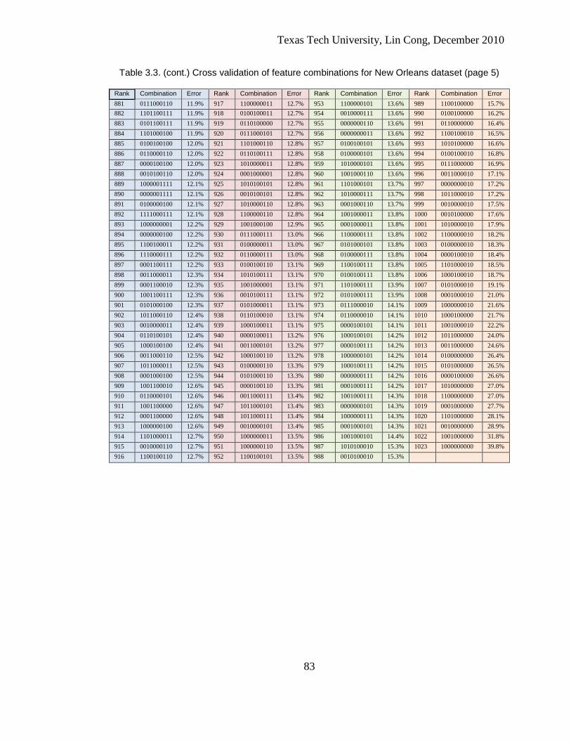
Texas Tech University, Lin Cong, December 2010
83
Table 3.3. (cont.) Cross validation of feature combinations for New Orleans dataset (page 5)
Rank Combination Error Rank Combination Error Rank Combination Error Rank Combination Error 881 0111000110 11.9% 917 1100000011 12.7% 953 1100000101 13.6% 989 1100100000 15.7% 882 1101100111 11.9% 918 0100100011 12.7% 954 0010000111 13.6% 990 0100100000 16.2% 883 0101100111 11.9% 919 0110100000 12.7% 955 0000000110 13.6% 991 0110000000 16.4% 884 1101000100 11.9% 920 0111000101 12.7% 956 0000000011 13.6% 992 1100100010 16.5% 885 0100100100 12.0% 921 1101000110 12.8% 957 0100100101 13.6% 993 1010100000 16.6% 886 0110000110 12.0% 922 0110100111 12.8% 958 0100000101 13.6% 994 0100100010 16.8% 887 0000100100 12.0% 923 1010000011 12.8% 959 1010000101 13.6% 995 0111000000 16.9% 888 0010100110 12.0% 924 0001000001 12.8% 960 1001000110 13.6% 996 0011000010 17.1% 889 1000001111 12.1% 925 1010100101 12.8% 961 1101000101 13.7% 997 0000000010 17.2% 890 0000001111 12.1% 926 0010100101 12.8% 962 1010000111 13.7% 998 1011000010 17.2% 891 0100000100 12.1% 927 1010000110 12.8% 963 0001000110 13.7% 999 0010000010 17.5% 892 1111000111 12.1% 928 1100000110 12.8% 964 1001000011 13.8% 1000 0010100000 17.6% 893 1000000001 12.2% 929 1001000100 12.9% 965 0001000011 13.8% 1001 1010000010 17.9% 894 0000000100 12.2% 930 0111000111 13.0% 966 1100000111 13.8% 1002 1100000010 18.2% 895 1100100011 12.2% 931 0100000011 13.0% 967 0101000101 13.8% 1003 0100000010 18.3% 896 1110000111 12.2% 932 0110000111 13.0% 968 0100000111 13.8% 1004 0000100010 18.4% 897 0001100111 12.2% 933 0100100110 13.1% 969 1100100111 13.8% 1005 1101000010 18.5% 898 0011000011 12.3% 934 1010100111 13.1% 970 0100100111 13.8% 1006 1000100010 18.7% 899 0001100010 12.3% 935 1001000001 13.1% 971 1101000111 13.9% 1007 0101000010 19.1% 900 1001100111 12.3% 936 0010100111 13.1% 972 0101000111 13.9% 1008 0001000010 21.0% 901 0101000100 12.3% 937 0101000011 13.1% 973 0111000010 14.1% 1009 1000000010 21.6% 902 1011000110 12.4% 938 0110100010 13.1% 974 0110000010 14.1% 1010 1000100000 21.7% 903 0010000011 12.4% 939 1000100011 13.1% 975 0000100101 14.1% 1011 1001000010 22.2% 904 0110100101 12.4% 940 0000100011 13.2% 976 1000100101 14.2% 1012 1011000000 24.0% 905 1000100100 12.4% 941 0011000101 13.2% 977 0000100111 14.2% 1013 0011000000 24.6% 906 0011000110 12.5% 942 1000100110 13.2% 978 1000000101 14.2% 1014 0100000000 26.4% 907 1011000011 12.5% 943 0100000110 13.3% 979 1000100111 14.2% 1015 0101000000 26.5% 908 0001000100 12.5% 944 0101000110 13.3% 980 0000000111 14.2% 1016 0000100000 26.6% 909 1001100010 12.6% 945 0000100110 13.3% 981 0001000111 14.2% 1017 1010000000 27.0% 910 0110000101 12.6% 946 0011000111 13.4% 982 1001000111 14.3% 1018 1100000000 27.0% 911 1001100000 12.6% 947 1011000101 13.4% 983 0000000101 14.3% 1019 0001000000 27.7% 912 0001100000 12.6% 948 1011000111 13.4% 984 1000000111 14.3% 1020 1101000000 28.1% 913 1000000100 12.6% 949 0010000101 13.4% 985 0001000101 14.3% 1021 0010000000 28.9% 914 1101000011 12.7% 950 1000000011 13.5% 986 1001000101 14.4% 1022 1001000000 31.8% 915 0010000110 12.7% 951 1000000110 13.5% 987 1010100010 15.3% 1023 1000000000 39.8% 916 1100100110 12.7% 952 1100100101 13.5% 988 0010100010 15.3%


![Web Performance Tuning Lin Wang, Ph.D. US Department of Education Copyright [Lin Wang] [2004]. This work is the intellectual property of the author. Permission.](https://static.fdocuments.in/doc/165x107/5518a32f550346b31f8b4960/web-performance-tuning-lin-wang-phd-us-department-of-education-copyright-lin-wang-2004-this-work-is-the-intellectual-property-of-the-author-permission.jpg)