Copyright © 2009 Pearson Education, Inc. Chapter 28 Analysis of Variance.

Copyright © 2009 Pearson Education, Inc.

Chapter 28

Analysis of Variance

3Copyright © 2009 Pearson Education, Inc.

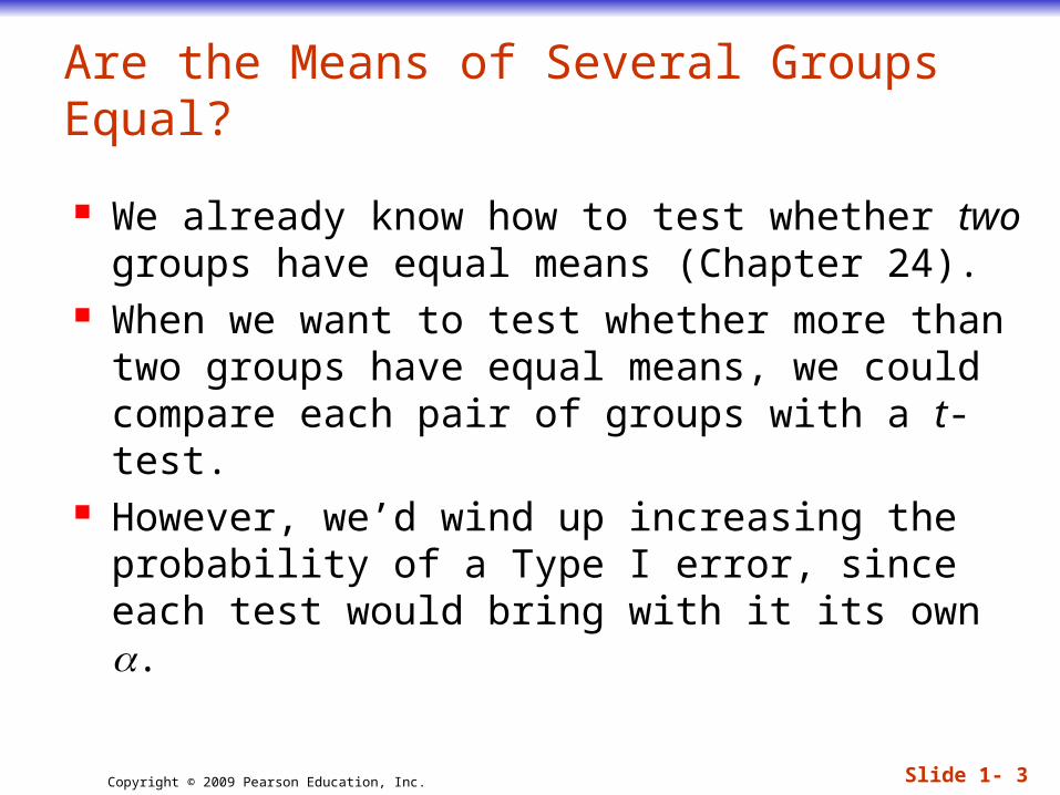
Are the Means of Several Groups Equal?

We already know how to test whether two groups have equal means (Chapter 24).

When we want to test whether more than two groups have equal means, we could compare each pair of groups with a t-test.

However, we’d wind up increasing the probability of a Type I error, since each test would bring with it its own .


Are the Means of Several Groups Equal? (cont.)

Fortunately, there is a test that generalizes the t-test to any number of treatment groups.

For comparing several means, there is yet another sampling distribution model, called the F-model.



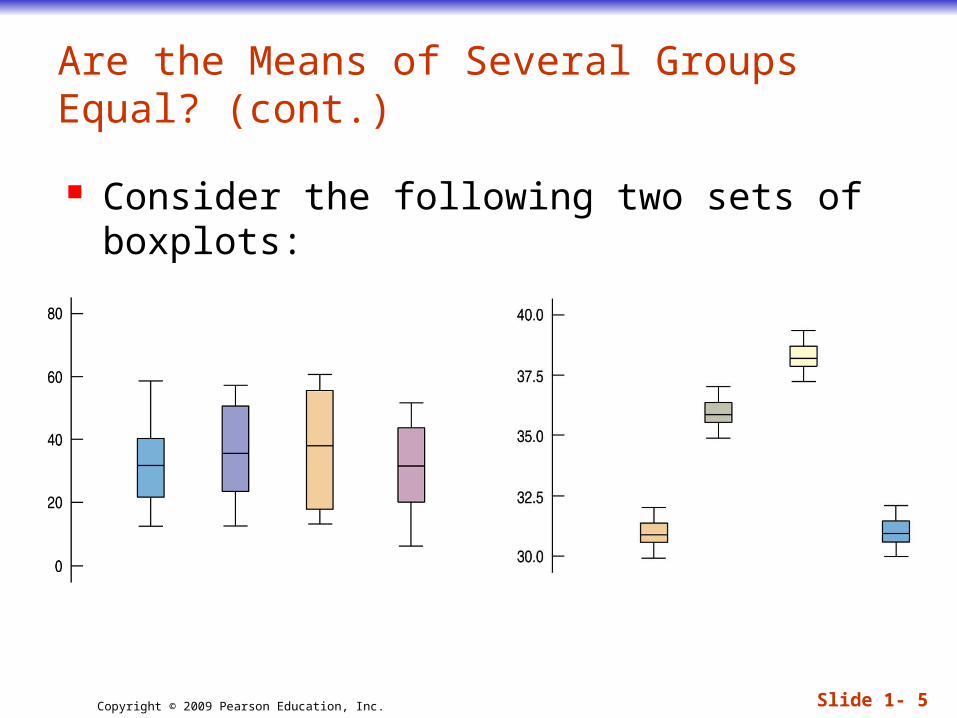
Consider the following two sets of boxplots:



It’s easy to see that the means in the second set differ. It’s hard to imagine that the means could be

that far apart just from natural sampling variability alone.

How about the first set? It looks like these observations could have occurred from treatments with the same means. This much variation among groups does seem

consistent with equal group means.



Believe it or not, the two sets of treatment means in both figures are the same. (They are 31, 36, 38, and 31, respectively.) Then why do the figures look so different?

In the second figure, the variation within each group is so small that the differences between the means stand out.

This is what we looked for when we compared boxplots by eye back in Chapter 5.



And it’s the central idea of the F-test. We compare the differences between the

means of the groups with the variation within the groups.

When the differences between means are large compared with the variation within the groups, we reject the null hypothesis and conclude that the means are (probably) not equal.

In the first figure, the differences among the means look as though they could have arisen just from natural sampling variability from groups with equal means, so there’s not enough evidence to reject H0.



How can we make this comparison more precise statistically?

All the tests we’ve seen have compared differences of some kind with a ruler based on an estimate of variation.

And we’ve always done that by looking at the ratio of the statistic to that variation estimate.

Here, the differences among the means will show up in the numerator, and the ruler we compare them with will be based on the underlying standard deviation—that is, on the variability within the treatment groups.


How Different Are They?

The key to our test will be thinking about the variation between groups.

If the null hypothesis is true, all the treatment means estimate the same underlying mean. The means we get for the groups would then

vary around the common mean only from natural sampling variation.

So, we could act as though the treatment means were just observations and find their variance.


How Different Are They? (cont.)

The more the means resemble each other, the smaller this variance will be; the more they differ, the larger this variance will be.

How much natural variation should we expect among the means if the null hypothesis is true?

If the null hypothesis were true, then each of the treatment means would estimate the same underlying mean.


How Different Are They? (cont.)

We can treat these estimated means as if they were observations and simply calculate their (sample) variance. This variance is the measure we’ll use to

assess how different the group means are from each other.

It’s the generalization of the difference between means for only two groups.

The more the group means resemble each other, the smaller this variance will be. The more they differ (perhaps because the treatments actually have an effect), the larger this variance will be.


The Ruler Within

We have an estimate from the variation within groups. That’s traditionally called the Error Mean Square (or sometimes Within Mean Square) and written MSE. It’s just the variance of the residuals. Because it’s a pooled variance, we write it .

We’ve got a separate estimate from the variation between the groups. We expect it to estimate 2 too, if we assume the null

hypothesis is true. We call this quantity the Treatment Mean Square (or sometimes Between Mean Square) denoted by MST.

sp2


The F-Statistic

When the null hypothesis is true and the treatment means are equal, both MSE and MST estimate 2, and their ratio should be close to 1.

We can use their ratio MST/MSE to test the null hypothesis: If the treatment means really are different, the

numerator will tend to be larger than the denominator, and the ratio will be bigger than 1.


The F-Statistic (cont.)

The sampling distribution model for this ratio, found by Sir Ronald Fisher, is called the F-distribution. We call the ratio MST/MSE the F-statistic.

By comparing the F-statistic to the appropriate F-distribution, we (or the computer) can get a P-value.



The test is one-tailed, because a larger difference in the treatments ultimately leads to a larger F-statistic. So the test is significant if the F-ratio is “big enough” (and the P-value “small enough”).

The entire analysis is called Analysis of Variance, commonly abbreviated ANOVA.



Just like Student’s t, the F-models are a family of distributions. However, since we have two variance estimates, we have two degrees of freedom parameters.

MST estimates the variance of the treatment means and has k – 1 degrees of freedom when there are k groups.

MSE is the pooled estimate of the variance within groups. If there are n observations in each of the k groups, MSE has k(n – 1) degrees of freedom.


The ANOVA Table

You’ll often see the Mean Squares and other information put into a table called the ANOVA table.

For the soap example in the book, the ANOVA table is:


The ANOVA Table (cont.)

The ANOVA table was originally designed to organize the calculations.

With advances in technology, we get all of this information, but we need only look at the F-ratio and the P-value.


The F-Table Usually, you’ll get the P-value for the F-statistic from

technology. Any software program performing an ANOVA will automatically “look up” the appropriate one-sided P-value for the F-statistic.

If you want to do it yourself, you’ll need an F-table. (There’s one at the end of the chapter called Table F.)

F-tables are usually printed only for a few values of a, often 0.05, 0.01, and 0.001.

They give the critical value of the F-statistic with the appropriate number of degrees of freedom determined by your data, for the -level that you select.


The F-Table (cont.)

If your F-statistic is greater than that value, you know that its P-value is less than that level.

So, you’ll be able to tell whether the P-value is greater or less than 0.05, 0.01, or 0.001, but to be more precise, you’ll need technology (or an interactive table like the one in ActivStats).


The F-Table (cont.)

Here’s an excerpt from an F-table for = 0.05:


The ANOVA Model

The text gives a detailed explanation of a model for understanding the ANOVA table. The student should study it carefully to fully understand the principles of the model and the table.


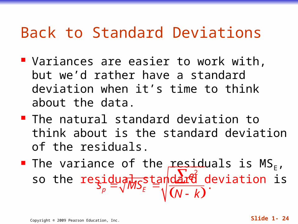
Back to Standard Deviations

Variances are easier to work with, but we’d rather have a standard deviation when it’s time to think about the data.

The natural standard deviation to think about is the standard deviation of the residuals.

The variance of the residuals is MSE, so the residual standard deviation is

sp MSE e2

N k .


Plot the Data…

First examine side-by-side boxplots of the data comparing the responses for all of the groups. Check for outliers within any of the groups (and

correct them if there are errors in the data). Get an idea of whether the groups have similar

spreads (as we’ll need). Get an idea of whether the centers seem to be

alike (as the null hypothesis claims) or different.

If the individual boxplots are all skewed in the same direction, consider re-expressing the response variable to make them more symmetric.


Assumptions and Conditions

As in regression, we must perform our checks of assumptions and conditions in order.

And, as in regression, displays of the residuals are often a good way to check the conditions for ANOVA.


Independence Assumptions The groups must be independent of each other.

No test can verify this assumption—you have to think about how the data were collected.

The data within each treatment group must be independent as well.

Check the Randomization Condition: Were the data collected with suitable randomization (a representative random sample or random assignment to treatment groups)?

Assumptions and Conditions (cont.)


Equal Variance Assumption ANOVA requires that the variances of the treatment

groups be equal. To check this assumption, we can check that the

groups have similar variances: Similar Variance Condition:

Look at side-by-side boxplots of the groups to see whether they have roughly the same spread.

Look at the original boxplots of the response values again—in general, do the spreads seem to change systematically with the centers? (This is more of a problem than random differences in spread among the groups and should not be ignored.)



Similar Variance Condition (cont): Look at the residuals plotted against the

predicted values. (Larger predicted values lead to larger magnitude residuals, indicating that the condition is violated.)



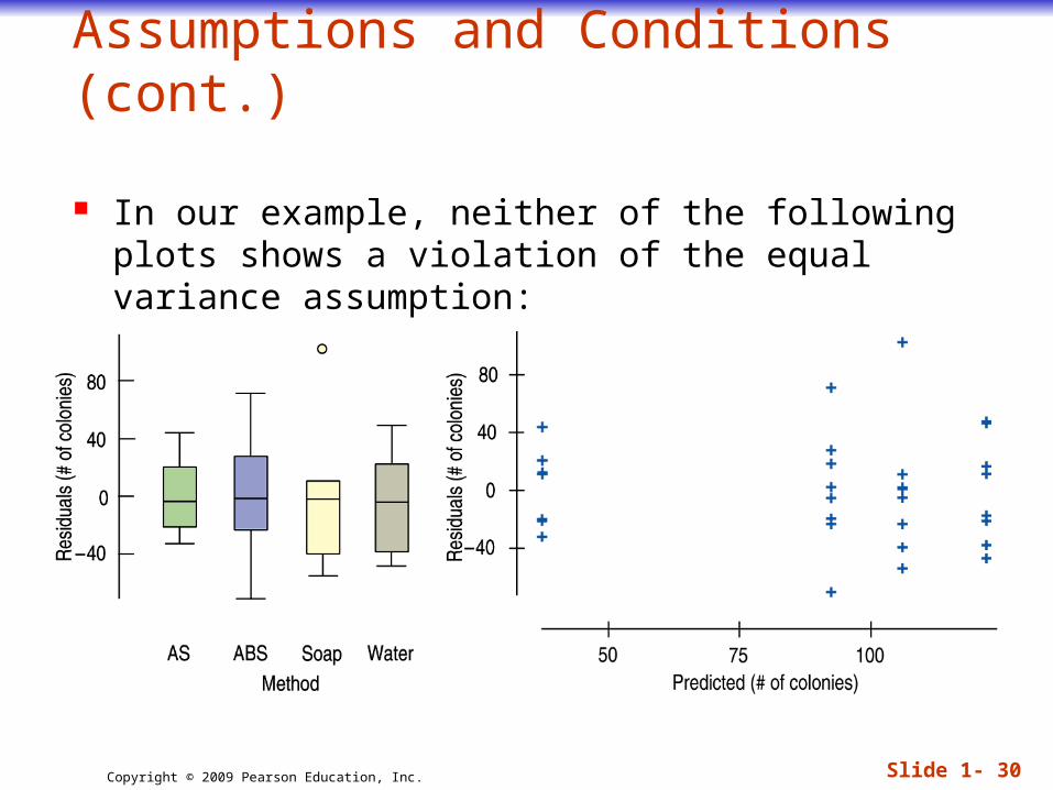
In our example, neither of the following plots shows a violation of the equal variance assumption:



Normal Population Assumption The F-test requires the underlying errors to follow a

Normal Model. We will check a corresponding Nearly Normal Condition:

examine a histogram of a Normal probability plot of all the residuals together.



Because we really care about the Normal model within each group, the Normal Population Assumption is violated if there are outliers in any of the groups. Check for outliers in the boxplots of the values

for each treatment group.



The Balancing Act

When we have an equal number of cases in each group, this is called balance.

Experiments that have equal numbers of experimental units in each treatment are said to be balanced or have balanced designs.

Balanced designs are a bit easier to analyze than unbalanced designs. But in the real world we often encounter unbalanced

data. Trust that technology will make the adjustments

necessary to analyze unbalanced designs.


Comparing Means

When we reject H0, it’s natural to ask which means are different. If we can’t reject the null, there’s nothing more

to do. If we’ve rejected the simple null hypothesis,

however, we can test whether any pairs or combinations of group means differ.

We could do a simple t-test about the difference between any pair of means. But, we could ask more complicated questions.


*Bonferroni Multiple Comparisons

We can’t just do multiple simple t-tests, since each test poses the risk of a Type I error. As we do more and more tests, the risk that we

might make a Type I error grows bigger than the level of each individual test.

If we do enough tests, we’re almost sure to reject one of the null hypotheses by mistake—and we’ll never know which one.


*Bonferroni Multiple Comparisons (cont.)

To defend against this problem, we will use a method for multiple comparisons. All multiple comparisons methods require that

we first reject the overall null hypothesis with the ANOVA’s F-test.

The margin of error that we have when testing any pair of means is called the least significant difference (LSD for short):

ME t sp1

n11

n2.


*Bonferroni Multiple Comparisons (cont.)

If two group means differ by more than this amount, then they are significantly different at level for each individual test.

We still have an issue with examining individual pairs. One way to combat this is with the Bonferroni method.

This method adjusts the LSD to allow for making many comparisons.

The result is a wider margin of error called the minimum significant difference (MSD).

The MSD is found by replacing t* with a t** that uses a confidence level of (1 - /J) instead of (1 - ) .


ANOVA on Observational Data When ANOVA is used to test equality of group means

from observational data, there’s no a priori reason to think the group variances might be equal at all. Even if the null hypothesis of equal means were

true, the groups might easily have different variances.

But if the side-by-side boxplots of responses for each group show roughly equal spreads and symmetric, outlier-free distributions, you can use ANOVA on observational data.

Be careful, though—if you have not assigned subjects to treatments randomly, you can’t draw causal conclusions even when the F-test is significant.


What Can Go Wrong?

Watch out for outliers. One outlier in a group can influence the entire

F-test and analysis. Watch out for changing variances.

If the conditions on the residuals are violated, it may be necessary to re-express the response variable to closer approximate the necessary conditions.


What Can Go Wrong? (cont.)

Be wary of drawing conclusions about causality from observational studies

Be wary of generalizing to situations other than the one at hand.

Watch out for multiple comparisons. Use a multiple comparisons method when you

want to test many pairs.


What have we learned?

We can compare the means of more than two independent groups based on samples drawn from those groups.

We’ve learned that under certain assumptions, the statistic used to test whether the means of groups are equal is distributed as an F-statistic with k – 1 and N – k degrees of freedom.

We’ve learned to check four conditions to verify the assumptions before we proceed.

We’ve learned that if an F-statistic is large enough, we reject the null hypothesis that all means are equal.

We’ve learned to create and interpret confidence intervals for the difference between each pair of group means.

Copyright © 2009 Pearson Education, Inc. Chapter 28 Analysis of Variance.

Documents

Transcript of Copyright © 2009 Pearson Education, Inc. Chapter 28 Analysis of Variance.