Copyright © 2009 Pearson Addison-Wesley. All rights reserved. Chapter 22 The Classical Foundations.
51
Copyright © 2009 Pearson Addison-Wesley. All rights reserved. Chapter 22 The Classical Foundations
-
Upload
myra-matthews -
Category
Documents
-
view
216 -
download
0
Transcript of Copyright © 2009 Pearson Addison-Wesley. All rights reserved. Chapter 22 The Classical Foundations.

Copyright © 2009 Pearson Addison-Wesley. All rights reserved.
Chapter 22
The Classical Foundations
Copyright © 2009 Pearson Addison-Wesley. All rights reserved. 22-2
Learning Objectives
• Define Say’s law and the classical understanding of aggregate supply
• Understand the supply of saving and demand for investment that leads to the equilibrium interest rate
• Explain the quantity theory of money and its implication for the aggregate demand curve
• Differentiate between nominal and real rate of interest
Copyright © 2009 Pearson Addison-Wesley. All rights reserved. 22-3
Introduction
• Origins of monetary theory lie in Classical Economics, starting with the works of Adam Smith (1723–1790)
• Two cornerstones of classical economics– Say’s Law—deals with interest rates, employment and
production
– Quantity Theory of Money—examines the role of money in the economy
• Focused on long-term view of the economy

Copyright © 2009 Pearson Addison-Wesley. All rights reserved. 22-4
Introduction (Cont.)
• Classical economics was attacked by John Maynard Keynes during the Great Depression
• Theory was resurrected and refined by modern monetarists and new classical macroeconomics beginning in the 1970s
• The starting point of classical theory is what determines gross domestic product (GDP)—total value of goods and services produced domestically

Copyright © 2009 Pearson Addison-Wesley. All rights reserved. 22-5
Classical Economics
• “Supply creates its own demand”
• The economy could never suffer from underemployment
• Total spending (demand) would always be sufficient to justify production at full employment (supply)
Copyright © 2009 Pearson Addison-Wesley. All rights reserved. 22-6
Classical Economics (Cont.)
• Potential output of an economy– Determined by the size of the labor force to work
with existing capital stock and level of technology (real factors in the economy)
– Production function defines the total supply of goods and services that can be produced
– Because of interplay of market forces (an invisible hand), production will always be at the full employment level
Copyright © 2009 Pearson Addison-Wesley. All rights reserved. 22-7
Classical Economics (Cont.)
• Potential output of an economy (Cont.)– Flexible wages and prices would assure that all markets
would clear—all goods sold and all people employed
– If the economy deviated from full employment, this flexibility would bring all markets back into equilibrium at the full employment level
– Laissez-faire—government intervention was not required
Copyright © 2009 Pearson Addison-Wesley. All rights reserved. 22-8
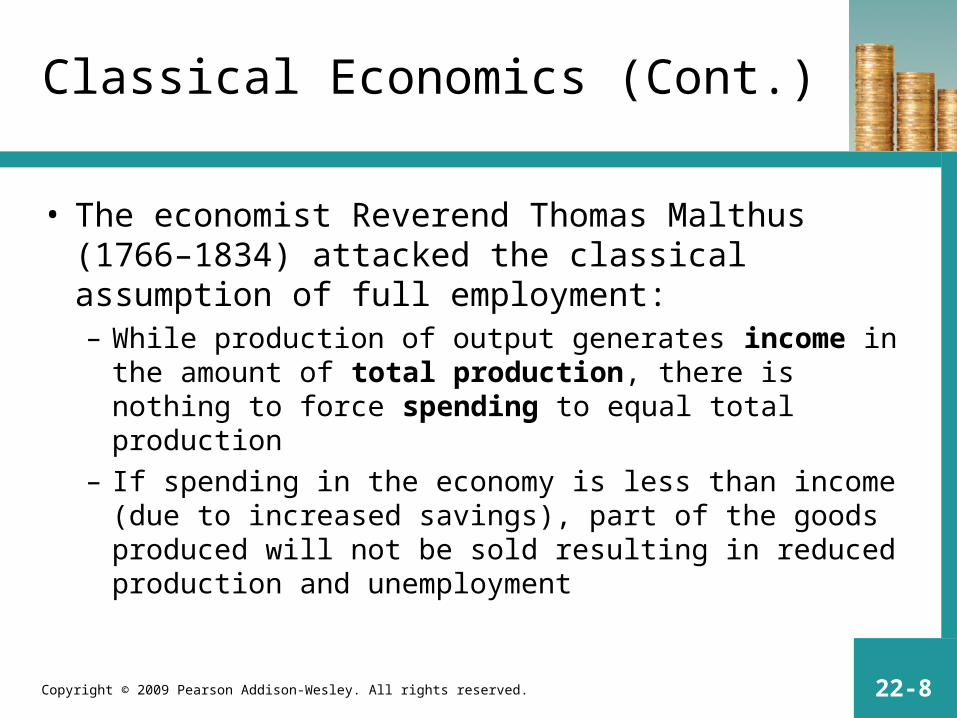
Classical Economics (Cont.)
• The economist Reverend Thomas Malthus (1766–1834) attacked the classical assumption of full employment:– While production of output generates income in the amount
of total production, there is nothing to force spending to equal total production
– If spending in the economy is less than income (due to increased savings), part of the goods produced will not be sold resulting in reduced production and unemployment

Copyright © 2009 Pearson Addison-Wesley. All rights reserved. 22-9
Classical Economics (Cont.)
• However, classical economists countered Malthus’s criticism:– Individuals save, but such funds do not disappear
– Savings are diverted from the spending stream, but flow to entrepreneurs to use for capital investment projects
– Savers receive interest on funds and borrowers are willing to pay as long as expected return on their investment exceeds the rate of interest
Copyright © 2009 Pearson Addison-Wesley. All rights reserved. 22-10
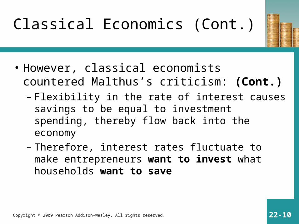
Classical Economics (Cont.)
• However, classical economists countered Malthus’s criticism: (Cont.)– Flexibility in the rate of interest causes savings to be
equal to investment spending, thereby flow back into the economy
– Therefore, interest rates fluctuate to make entrepreneurs want to invest what households want to save

Copyright © 2009 Pearson Addison-Wesley. All rights reserved. 22-11
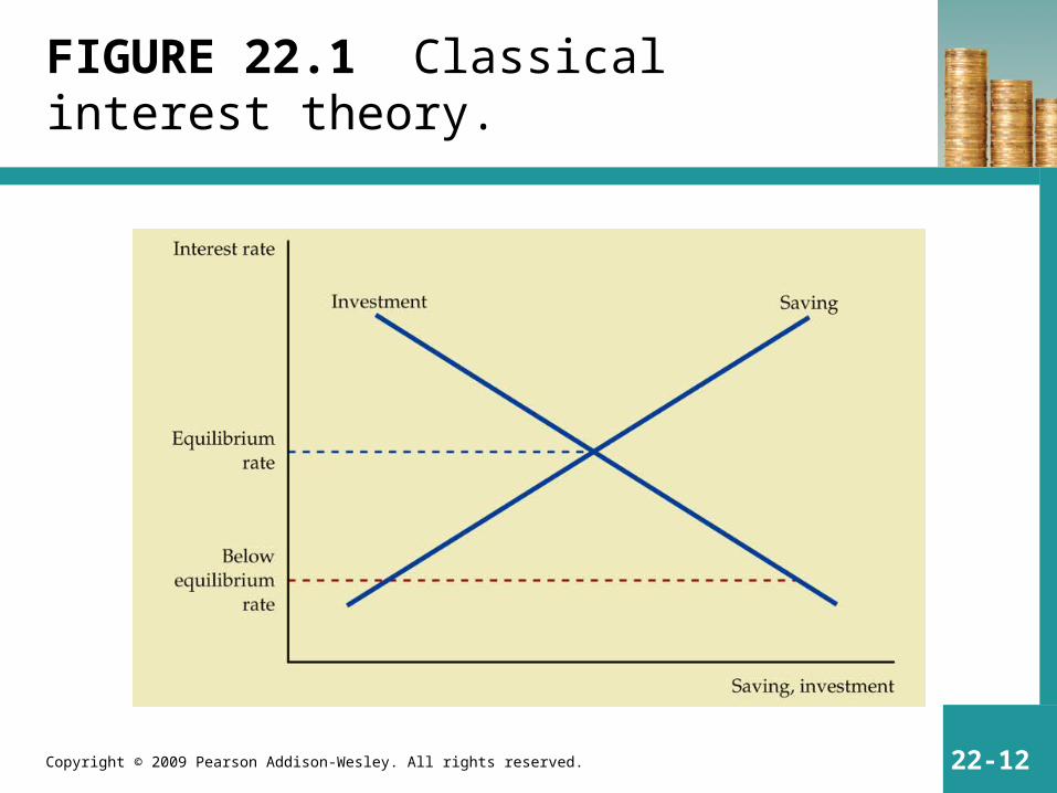
Classical Interest Theory
• Overall level of interest rates is determined by supply and demand for loanable funds (Figure 22.1)
• However, classical economics focused on savings and investment, the two factors that underlie the long-run supply and demand for loanable funds
Copyright © 2009 Pearson Addison-Wesley. All rights reserved. 22-12
FIGURE 22.1 Classical interest theory.
Copyright © 2009 Pearson Addison-Wesley. All rights reserved. 22-13
Classical Interest Theory (Cont.)
• Savings (Figure 22.1)– Function of interest rates—the higher the rate of
interest, the more will be saved (positive or direct relation)
– Interest earned on savings is a reward for delaying consumption in favor of future consumption
– At higher interest rates people will be more willing to forgo present consumption
Copyright © 2009 Pearson Addison-Wesley. All rights reserved. 22-14
Classical Interest Theory (Cont.)
• Investment (Figure 22.1)– Also a function of interest rates—the lower the rate of
interest, the more entrepreneurs will borrow and invest (negative or indirect relation)
– Investment in physical capital is undertaken because capital goods produce output in the future
– The firm will undertake the investment if the rate of return exceeds the cost of borrowing

Copyright © 2009 Pearson Addison-Wesley. All rights reserved. 22-15
Classical Interest Theory (Cont.)
• Investment (Figure 22.1)– The return on investments is subject to diminishing
returns, each successive project earns a lower return on investment
– Therefore, a lower rate of interest induces entrepreneurs to undertake more and more investments

Copyright © 2009 Pearson Addison-Wesley. All rights reserved. 22-16
Classical Interest Theory (Cont.)
• Equilibrium rate of interest (Figure 22.1)– Represented by the intersection of the supply/demand curve
for loanable funds
– Total savings is equal to total investment
– That portion of income that was diverted from spending to savings flows back into the spending stream in the form of investment
– As long as the supply or demand for loanable funds do not shift, this equilibrium rate of interest will not change

Copyright © 2009 Pearson Addison-Wesley. All rights reserved. 22-17
Classical Interest Theory (Cont.)
• Shifts in supply or demand (Figure 22.2)– Any shift in the supply or demand for loanable funds
will cause market forces to drive the rate of interest back into equilibrium at a different level
– This flexibility in the rate of interest will ensure that the amount of savings is always equal to investment and total income will always equal total spending

Copyright © 2009 Pearson Addison-Wesley. All rights reserved. 22-18
FIGURE 22.2 Increased saving calls forth increased investment.
Copyright © 2009 Pearson Addison-Wesley. All rights reserved. 22-19
Classical Interest Theory (Cont.)
• Role of money in determining interest rate – Rate of interest is influenced in the long run by the savings of
the public (personal preferences) and investment of entrepreneurs (productivity of capital)
– Money plays no role in determining real factors in the classical system
– Real factors are determined by the supply of capital, the labor force, and existing technology
– Interest rates are determined by the thriftiness of the public and the productivity of capital

Copyright © 2009 Pearson Addison-Wesley. All rights reserved. 22-20
Quantity Theory of Money
• In classical economics, money is strictly a veil—it affects the price level, but not the real factors in the economy
• Increase in money will lead only to increase in prices, but not output or employment

Copyright © 2009 Pearson Addison-Wesley. All rights reserved. 22-21
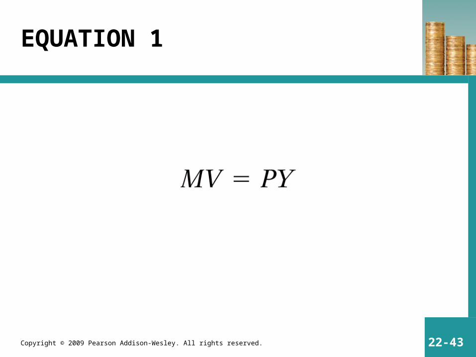
Quantity Theory of Money (Cont.)
• Equation of Exchange– M V = P Y
• Where: M = money supply
• V = Income velocity (rate of turnover)
• P = price level
• Y = real income (GDP)

Copyright © 2009 Pearson Addison-Wesley. All rights reserved. 22-22
Quantity Theory of Money (Cont.)
• Equation of Exchange (Cont.)– This expression is a truism—true by definition
– Generally, “Y” is referred to as real gross domestic product (GDP)
– The price level “P” is an index of the current prices of all goods (CPI)
– The product of “Y P” represents the nominal level of GDP
– This equation equates total spending (left hand) with total purchases (right hand)

Copyright © 2009 Pearson Addison-Wesley. All rights reserved. 22-23
Quantity Theory of Money (Cont.)
• Equation of Exchange (Cont.)– Originally this equation was expressed in terms of
“T”, the total level of transactions– Includes both real and financial assets– In this expression, “V” is called the transactions
velocity– The remainder of this discussion will be in terms of
the income velocity
Copyright © 2009 Pearson Addison-Wesley. All rights reserved. 22-24
Quantity Theory of Money (Cont.)
• The Cambridge Approach– Restates equation of exchange to focus on fraction of total
expenditure people hold as money
– Manipulation of the equation of exchange results in the Cambridge cash-balance approach or the demand-for-money equation
• M = kPY– Where: k = fraction of spending that people have command over in the
form of money balances
– Since “k” = 1/V, both the equation of exchange and the cash-balance approach are identical

Copyright © 2009 Pearson Addison-Wesley. All rights reserved. 22-25
Quantity Theory of Money (Cont.)
• Quantity Theory of Money– Re-interprets equation of exchange as a behavioral
relationship—an increase in quantity of money (M) causes what changes in other variables
– According to the quantity theory of money, a change in the money supply leads to a proportionate change in the price level (cause-and-effect conclusion)

Copyright © 2009 Pearson Addison-Wesley. All rights reserved. 22-26
Quantity Theory of Money (Cont.)
• Quantity Theory of Money (Cont.)– The above is based on two propositions:
• “Y” is assumed fixed at full employment levels• “V” is assumed fixed by payment habits of the population
– The transmission mechanism of an increase in the money supply is as follows:
• Money supply increases• Individuals now hold larger cash balances• Reduce cash balances by spending on goods/services• Since output (Y) [real GDP] is fixed, the increased demand drives up
prices with no increase in real output
Copyright © 2009 Pearson Addison-Wesley. All rights reserved. 22-27
Quantity Theory of Money (Cont.)
• Quantity Theory of Money (Cont.)– Therefore, a change in the money supply leaves the
real amount of goods and services produced (real GDP) unchanged, but increases the dollar value of GDP (nominal GDP)
– Money is a veil in the economy and has no effect on real output or employment levels
Copyright © 2009 Pearson Addison-Wesley. All rights reserved. 22-28
Money Demand and the Quantity Theory
• When explaining transmission mechanism, cash-balance version (M = kPY) is superior
• The fraction of nominal GDP (PY) people want to hold in the form of money, k, is determined by many forces– It is essentially a transactions demand for money
– Since money is a medium of exchange, the value of k is influenced by the frequency of receipts and expenditures

Copyright © 2009 Pearson Addison-Wesley. All rights reserved. 22-29
Money Demand and the Quantity Theory (Cont.)
• Fraction of nominal GDP held as cash (Cont.)– The ease you can buy on credit also influences k by
permitting people to reduce the average balances in their checking accounts
– Money is used as a temporary abode of purchasing power—waiting until an individual wants to spend on real goods or services
– Although the value of k may vary by individuals, for the population as a whole it appears to be rather stable

Copyright © 2009 Pearson Addison-Wesley. All rights reserved. 22-30
Money Demand and the Quantity Theory (Cont.)
• If the money supply increases:– Individuals hold larger cash balances and spend it on real
goods and services
– Spending will stop when nominal balances have increased proportionately through price increases
– Therefore, the real value of money (M/P) held is the same in both the initial and final position
– The increase in money must result in an equal percentage in prices for the real value of money to be in equilibrium

Copyright © 2009 Pearson Addison-Wesley. All rights reserved. 22-31
Aggregate Demand and Supply: A Summary
• Figure 22.3– Price (index of all prices) is measured on the vertical and
quantity (real aggregate output) is on the horizontal
– Since output and income are identical in the classical theory, the terms income and output are interchangeable
– Aggregate supply curve• Perfectly vertical at the full employment level of output
• Does not vary with the price level

Copyright © 2009 Pearson Addison-Wesley. All rights reserved. 22-32
FIGURE 22.3 The equilibrium price level.
Copyright © 2009 Pearson Addison-Wesley. All rights reserved. 22-33
Aggregate Demand and Supply: A Summary (Cont.)
• Figure 22.3 (Cont.)– Aggregate demand curve
• Downward sloping
• Drawn for a given level of the money supply (M)
• Hence, a lower price level means that the amount of goods and services demanded is greater
– Intersection of the supply and demand curve• Indicates the equilibrium price level
• Flexibility of prices means that a change in aggregate demand will result in only a change of price at a constant level of output

Copyright © 2009 Pearson Addison-Wesley. All rights reserved. 22-34
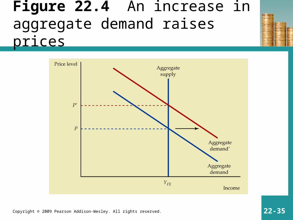
Aggregate Demand and Supply: A Summary (Cont.)
• Figure 22.4– This shows the effect of shifting the demand curve to
the right by an increase in the money supply– Before the increase of M, individuals held the right
amount of real cash balances at price P– However, when the money supply increases, people
now hold too large real cash balances– They spend until the price increases to P’ and
equilibrium of real cash balances has been restored
Copyright © 2009 Pearson Addison-Wesley. All rights reserved. 22-35
Figure 22.4 An increase in aggregate demand raises prices
Copyright © 2009 Pearson Addison-Wesley. All rights reserved. 22-36
Aggregate Demand and Supply: A Summary (Cont.)
• Figure 22.4 (Cont.)– Continued expansion of the money supply results in
increasing prices (inflation), but not in increased real output
– Therefore, in classic economic theory, inflation is a monetary phenomenon and only supported by ever increasing money supply

Copyright © 2009 Pearson Addison-Wesley. All rights reserved. 22-37
Real Versus Nominal Rates of Interest
• With the possibility of inflation, it is necessary to make a distinction between the real rate of interest and the nominal rate
• Inflation erodes the real purchasing power of income earned at a given nominal rate of interest
• Real interest = nominal interest – anticipated inflation
Copyright © 2009 Pearson Addison-Wesley. All rights reserved. 22-38
Real Versus Nominal Rates of Interest (Cont.)
• Savers and investors will factor inflation when considering whether to save/invest at a given level of nominal interest
• Increasing expectations of inflation will drive the nominal interest rate up until the real interest rate is at the level determined by savings and investment
• Therefore, inflation will not cause the real rate of interest to change

Copyright © 2009 Pearson Addison-Wesley. All rights reserved. 22-39
Modern Modifications: Monetarists and New Classicists
• Modifications to the classical economic theory were developed at the University of Chicago starting in the late 1940s
• Monetarists– Adhere to virtually all tenets of classical economics– However, they have made some modifications– They focus on the relationship between M and PY
rather than just M and P
Copyright © 2009 Pearson Addison-Wesley. All rights reserved. 22-40
Modern Modifications: Monetarists and New Classicists (Cont.)
• Monetarists (Cont.)– Recognizes the fact that real output may deviate temporarily
from full employment, however, eventually the economy will tend toward the full employment level of output
– In the 1950s, Milton Friedman replaced the idea of the stability of velocity with a less restrictive notion that it varies in a predictable manner
– Money demand may not be a fixed fraction of total spending, but is related to PY in a close and predictable way

Copyright © 2009 Pearson Addison-Wesley. All rights reserved. 22-41
Modern Modifications: Monetarists and New Classicists (Cont.)
• Monetarists (Cont.)– Therefore, in the short run an increase in M might lead to
temporary higher real output, but eventually is reflected just in higher prices
– Since the monetarists upheld the classical tradition of inherent stability of the economy at full employment, they rejected governmental attempts to fine-tune the economy
– Governmental intervention is unnecessary to regulate the economy and may be potentially damaging
Copyright © 2009 Pearson Addison-Wesley. All rights reserved. 22-42
Modern Modifications: Monetarists and New Classicists (Cont.)
• New Classical Macroeconomists– Added another reason for futility of government efforts at
fine-tuning the economy
– Rational Expectations• People formulate expectations based on all available information and
recognize that the economy will always tend toward full employment
• Therefore, attempts to reduce unemployment by increasing the money supply will not be successful since people will immediately drive up prices
• No real effect on economy, just higher prices
Copyright © 2009 Pearson Addison-Wesley. All rights reserved. 22-43
EQUATION 1

Copyright © 2009 Pearson Addison-Wesley. All rights reserved. 22-44
EQUATION 2

Copyright © 2009 Pearson Addison-Wesley. All rights reserved. 22-45
EQUATION 3
Copyright © 2009 Pearson Addison-Wesley. All rights reserved.
Appendix
GDP DEFINITIONS AND RELATIONSHIPS
Copyright © 2009 Pearson Addison-Wesley. All rights reserved. 22-47
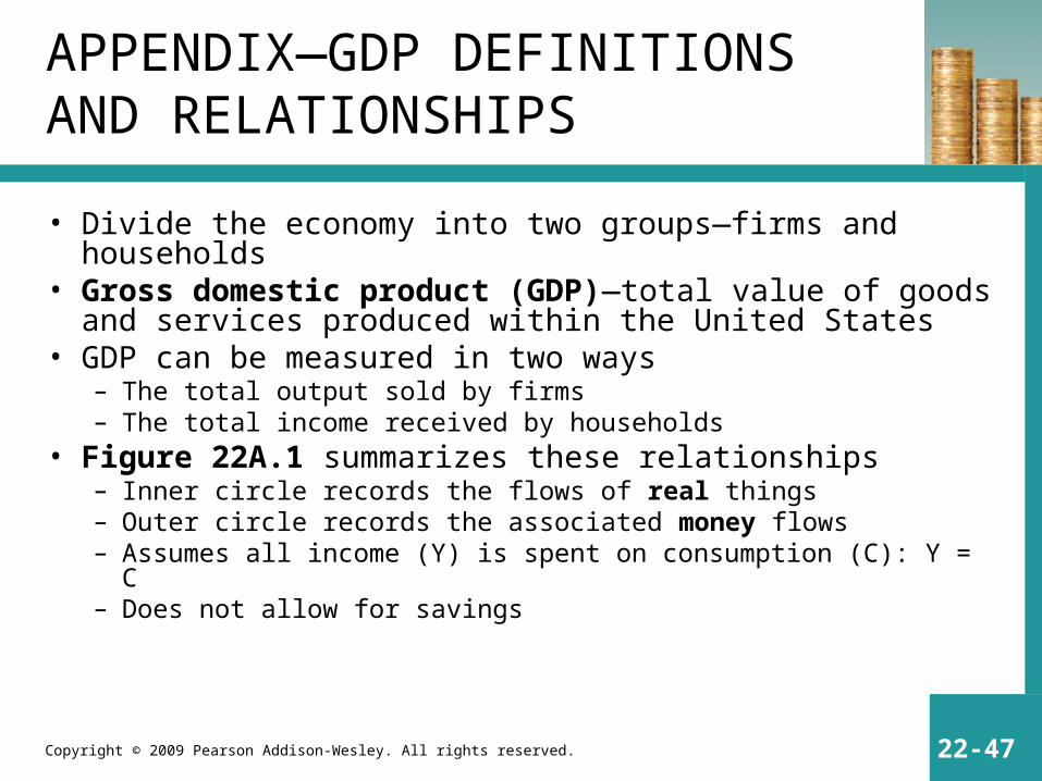
APPENDIX—GDP DEFINITIONS AND RELATIONSHIPS
• Divide the economy into two groups—firms and households• Gross domestic product (GDP)—total value of goods and
services produced within the United States• GDP can be measured in two ways
– The total output sold by firms– The total income received by households
• Figure 22A.1 summarizes these relationships– Inner circle records the flows of real things – Outer circle records the associated money flows – Assumes all income (Y) is spent on consumption (C): Y = C– Does not allow for savings
Copyright © 2009 Pearson Addison-Wesley. All rights reserved. 22-48
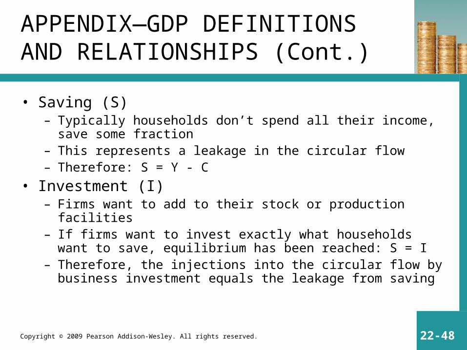
APPENDIX—GDP DEFINITIONS AND RELATIONSHIPS (Cont.)
• Saving (S)– Typically households don’t spend all their income, save some fraction– This represents a leakage in the circular flow– Therefore: S = Y - C
• Investment (I)– Firms want to add to their stock or production facilities – If firms want to invest exactly what households want to save, equilibrium
has been reached: S = I– Therefore, the injections into the circular flow by business investment
equals the leakage from saving
Copyright © 2009 Pearson Addison-Wesley. All rights reserved. 22-49
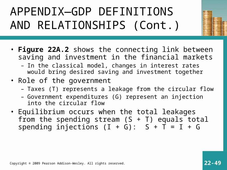
APPENDIX—GDP DEFINITIONS AND RELATIONSHIPS (Cont.)
• Figure 22A.2 shows the connecting link between saving and investment in the financial markets– In the classical model, changes in interest rates would bring desired
saving and investment together
• Role of the government– Taxes (T) represents a leakage from the circular flow– Government expenditures (G) represent an injection into the circular flow
• Equilibrium occurs when the total leakages from the spending stream (S + T) equals total spending injections (I + G): S + T = I + G

Copyright © 2009 Pearson Addison-Wesley. All rights reserved. 22-50
FIGURE 22A.1 The circular flow of spending, income, and output.

Copyright © 2009 Pearson Addison-Wesley. All rights reserved. 22-51
FIGURE 22A.2 The circular flow including saving and investment.


![INTERACTION PARADIGMS Based on: S. Heim, The Resonant Interface HCI Foundations for Interaction Design [Chapter 1] Addison-Wesley, 2007 [slides from S.](https://static.fdocuments.in/doc/165x107/56649cd85503460f949a1d02/interaction-paradigms-based-on-s-heim-the-resonant-interface-hci-foundations.jpg)


![INTERACTION STYLES References S. Heim, The Resonant Interface HCI Foundations for Interaction Design [Chapter 2] Addison-Wesley, 2007 J. Preece, Y. Rogers,](https://static.fdocuments.in/doc/165x107/5697bf731a28abf838c7f4d8/interaction-styles-references-s-heim-the-resonant-interface-hci-foundations.jpg)