Copyright © 2005 Brooks/Cole, a division of Thomson Learning, Inc. 8.1 Chapter 8 Continuous...
30
8.1 Copyright © 2005 Brooks/Cole, a division of Thomson Learning, Inc. Chapter 8 Continuous Probability Distributions
-
Upload
austin-lawson -
Category
Documents
-
view
264 -
download
2
Transcript of Copyright © 2005 Brooks/Cole, a division of Thomson Learning, Inc. 8.1 Chapter 8 Continuous...

8.1Copyright © 2005 Brooks/Cole, a division of Thomson Learning, Inc.
Chapter 8
Continuous Probability Distributions
8.2Copyright © 2005 Brooks/Cole, a division of Thomson Learning, Inc.
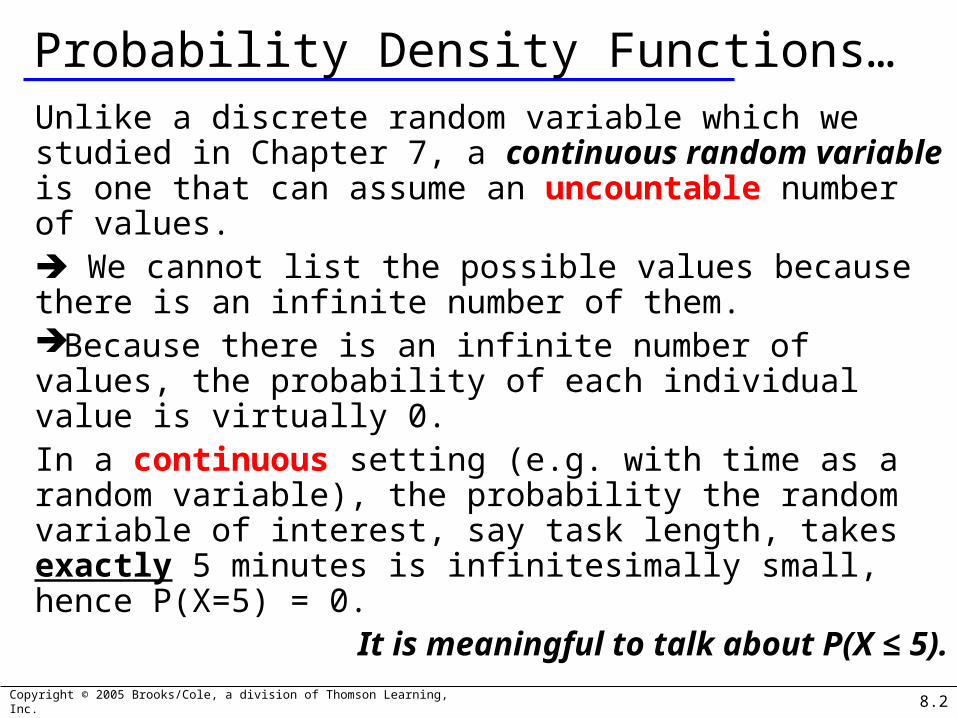
Probability Density Functions…Unlike a discrete random variable which we studied in Chapter 7, a continuous random variable is one that can assume an uncountable number of values. We cannot list the possible values because there is an infinite number of them.Because there is an infinite number of values, the probability of each individual value is virtually 0.In a continuous setting (e.g. with time as a random variable), the probability the random variable of interest, say task length, takes exactly 5 minutes is infinitesimally small, hence P(X=5) = 0.
It is meaningful to talk about P(X ≤ 5).
8.3Copyright © 2005 Brooks/Cole, a division of Thomson Learning, Inc.
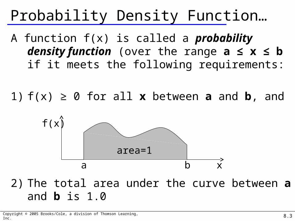
Probability Density Function…
A function f(x) is called a probability density function (over the range a ≤ x ≤ b if it meets the following requirements:
1) f(x) ≥ 0 for all x between a and b, and
2) The total area under the curve between a and b is 1.0
f(x)
xba
area=1

8.4Copyright © 2005 Brooks/Cole, a division of Thomson Learning, Inc.
The Normal Distribution…
The normal distribution is the most important of all probability distributions. The probability density function of a normal random variable is given by:
It looks like this:
Bell shaped,
Symmetrical around the mean …

8.5Copyright © 2005 Brooks/Cole, a division of Thomson Learning, Inc.
The Normal Distribution…
Important things to note:
The normal distribution is fully defined by two parameters:its standard deviation and mean
Normal distributions range from minus infinity to plus infinity
The normal distribution is bell shaped andsymmetrical about the mean

8.6Copyright © 2005 Brooks/Cole, a division of Thomson Learning, Inc.
Standard Normal Distribution…
A normal distribution whose mean is zero and standard deviation is one is called the standard normal distribution.
As we shall see shortly, any normal distribution can be converted to a standard normal distribution with simple algebra. This makes calculations much easier.
0
1
1
8.7Copyright © 2005 Brooks/Cole, a division of Thomson Learning, Inc.
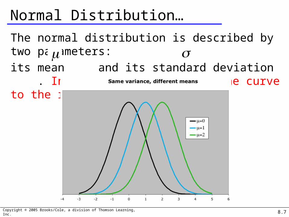
Normal Distribution…
The normal distribution is described by two parameters:
its mean and its standard deviation . Increasing the mean shifts the curve to the right…
8.8Copyright © 2005 Brooks/Cole, a division of Thomson Learning, Inc.
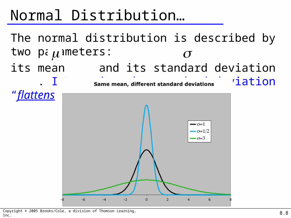
Normal Distribution…
The normal distribution is described by two parameters:
its mean and its standard deviation . Increasing the standard deviation “flattens” the curve…

8.9Copyright © 2005 Brooks/Cole, a division of Thomson Learning, Inc.
Calculating Normal Probabilities…
We can use the following function to convert any normal random variable to a standard normal random variable…
Some advice: always draw a
picture!
0

8.10Copyright © 2005 Brooks/Cole, a division of Thomson Learning, Inc.
Calculating Normal Probabilities…
Example: The time required to build a computer is normally distributed with a mean of 50 minutes and a standard deviation of 10 minutes:
What is the probability that a computer is assembled in a time between 45 and 60 minutes?
Algebraically speaking, what is P(45 < X < 60) ?
0

8.11Copyright © 2005 Brooks/Cole, a division of Thomson Learning, Inc.
Calculating Normal Probabilities…
P(45 < X < 60) ?
0
…mean of 50 minutes and astandard deviation of 10 minutes…
8.12Copyright © 2005 Brooks/Cole, a division of Thomson Learning, Inc.
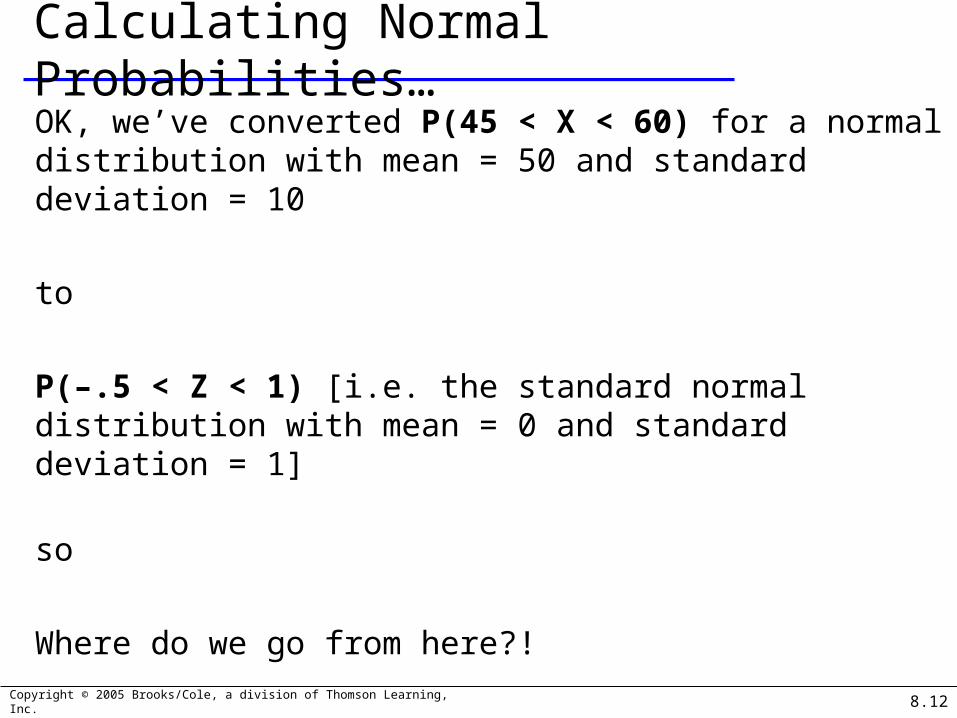
Calculating Normal Probabilities…
OK, we’ve converted P(45 < X < 60) for a normal distribution with mean = 50 and standard deviation = 10
to
P(–.5 < Z < 1) [i.e. the standard normal distribution with mean = 0 and standard deviation = 1]
so
Where do we go from here?!

8.13Copyright © 2005 Brooks/Cole, a division of Thomson Learning, Inc.
Calculating Normal Probabilities…
P(–.5 < Z < 1) looks like this:
The probability is the area
under the curve…
We will add up the
two sections:
P(–.5 < Z < 0) and
P(0 < Z < 1)
We can use Table 3 in Appendix B to look-up probabilities P(Z < z)
0
–.5 … 1

8.14Copyright © 2005 Brooks/Cole, a division of Thomson Learning, Inc.
Calculating Normal Probabilities…
Recap: The time required to build a computer is normally distributed with a mean of 50 minutes and a standard deviation of 10 minutesWhat is the probability that a computer is assembled in a time between 45 and 60 minutes?
P(45 < X < 60) = P(–.5 < Z < 1) = .5328
“Just over half the time, 53% or so, a computer will have an assembly time between 45 minutes and 1 hour”
8.15Copyright © 2005 Brooks/Cole, a division of Thomson Learning, Inc.
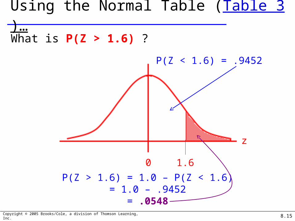
Using the Normal Table (Table 3)…
What is P(Z > 1.6) ?
0 1.6
P(Z < 1.6) = .9452
P(Z > 1.6) = 1.0 – P(Z < 1.6)= 1.0 – .9452
= .0548
z

8.16Copyright © 2005 Brooks/Cole, a division of Thomson Learning, Inc.
Using the Normal Table (Table 3)…
What is P(0.9 < Z < 1.9) ?
0 0.9
P(Z < 0.9)
P(0.9 < Z < 1.9) = P(Z < 1.9) – P(Z < 0.9)=.9713 – .8159
= .1554
z
1.9
P(Z < 1.9)
8.17Copyright © 2005 Brooks/Cole, a division of Thomson Learning, Inc.
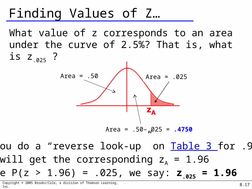
Finding Values of Z…
What value of z corresponds to an area under the curve of 2.5%? That is, what is z.025 ?
Area = .50 Area = .025
Area = .50–.025 = .4750
If you do a “reverse look-up” on Table 3 for .9750,you will get the corresponding zA = 1.96Since P(z > 1.96) = .025, we say: z.025 = 1.96

8.18Copyright © 2005 Brooks/Cole, a division of Thomson Learning, Inc.
Finding Values of Z…
Other Z values are
Z.05 = 1.645
Z.01 = 2.33

8.19Copyright © 2005 Brooks/Cole, a division of Thomson Learning, Inc.
Using the values of Z
Because z.025 = 1.96 and - z.025= -1.96, it follows that we can state
P(-1.96 < Z < 1.96) = .95
Recall that the empirical rule stated that approximately 95% would be within + 2 standard deviations. From now on we use 1.96 instead of 2.
Similarly
P(-1.645 < Z < 1.645) = .90

8.20Copyright © 2005 Brooks/Cole, a division of Thomson Learning, Inc.
Other Continuous Distributions…
Three other important continuous distributions which will be used extensively in later sections are introduced here:
Student t Distribution, [will use in this class]
Chi-Squared Distribution,
F Distribution, [will use in this class]
Exponential.

8.21Copyright © 2005 Brooks/Cole, a division of Thomson Learning, Inc.
Student t Distribution…
Much like the standard normal distribution, the Student t distribution is “mound” shaped and symmetrical about its mean of zero: Looks like the normal distribution after an elephant sat on it [flattened out/spread out more than a normal]
8.22Copyright © 2005 Brooks/Cole, a division of Thomson Learning, Inc.
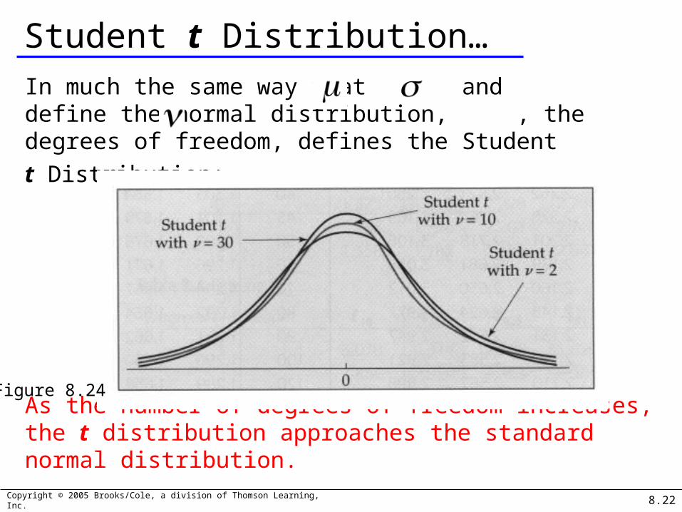
Student t Distribution…
In much the same way that and define the normal distribution, , the degrees of freedom, defines the Student
t Distribution:
As the number of degrees of freedom increases, the t distribution approaches the standard normal distribution.
Figure 8.24
8.23Copyright © 2005 Brooks/Cole, a division of Thomson Learning, Inc.
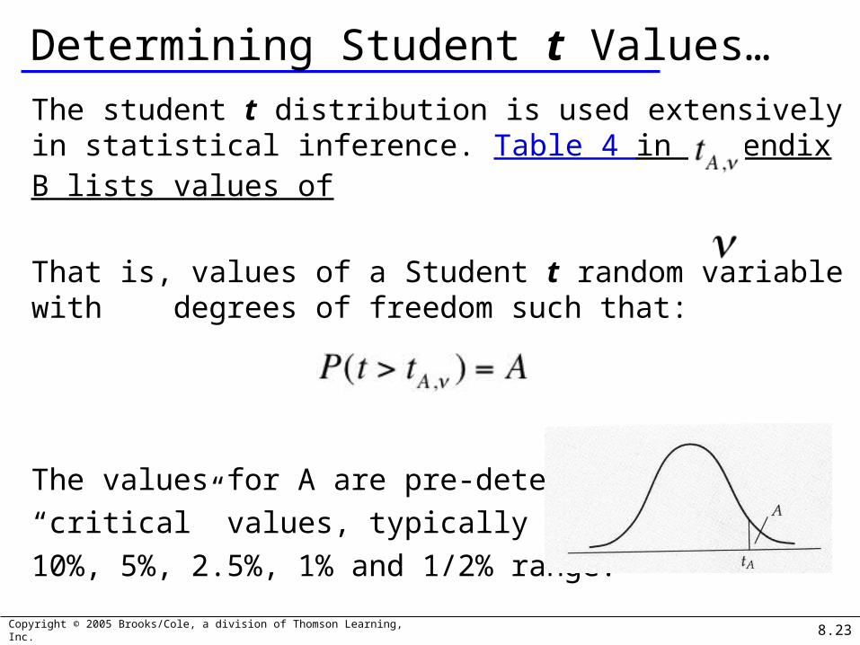
Determining Student t Values…
The student t distribution is used extensively in statistical inference. Table 4 in Appendix B lists values of
That is, values of a Student t random variable with degrees of freedom such that:
The values for A are pre-determined
“critical” values, typically in the
10%, 5%, 2.5%, 1% and 1/2% range.
8.24Copyright © 2005 Brooks/Cole, a division of Thomson Learning, Inc.
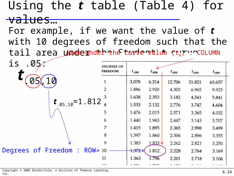
Using the t table (Table 4) for values…For example, if we want the value of t with 10 degrees of freedom such that the tail area under the Student t curve is .05: Area under the curve value (tA) : COLUMN
Degrees of Freedom : ROW
t.05,10
t.05,10=1.812
8.25Copyright © 2005 Brooks/Cole, a division of Thomson Learning, Inc.
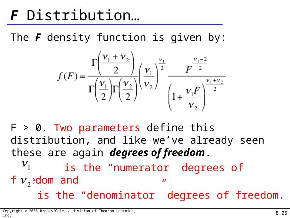
F Distribution…
The F density function is given by:
F > 0. Two parameters define this distribution, and like we’ve already seen these are again degrees of freedom.
is the “numerator” degrees of freedom and
is the “denominator” degrees of freedom.
8.26Copyright © 2005 Brooks/Cole, a division of Thomson Learning, Inc.
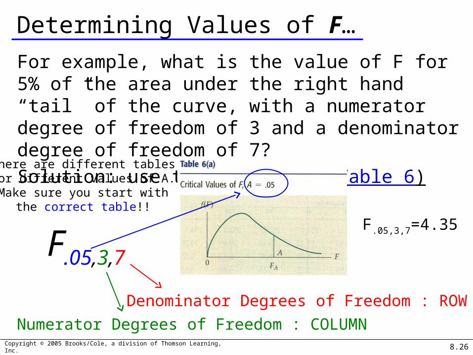
Determining Values of F…
For example, what is the value of F for 5% of the area under the right hand “tail” of the curve, with a numerator degree of freedom of 3 and a denominator degree of freedom of 7?
Solution: use the F look-up (Table 6)
Numerator Degrees of Freedom : COLUMN
Denominator Degrees of Freedom : ROW
F.05,3,7
There are different tablesfor different values of A.Make sure you start with
the correct table!!
F.05,3,7=4.35

8.27Copyright © 2005 Brooks/Cole, a division of Thomson Learning, Inc.
Problem: Normal Distribution
If the random variable Z has a standard normal distribution, calculate the following probabilities.
P(Z > 1.7) =
P(Z < 1.7) =
P(Z > -1.7) =
P(Z < -1.7) =
P(-1.7 < Z < 1.7)

8.28Copyright © 2005 Brooks/Cole, a division of Thomson Learning, Inc.
Problem: Normal
If the random variable X has a normal distribution with
mean 40 and std. dev. 5, calculate the following
probabilities.P(X > 43) =
P(X < 38) =
P(X = 40) =
P(X > 23) =

8.29Copyright © 2005 Brooks/Cole, a division of Thomson Learning, Inc.
Problem: Normal
The time (Y) it takes your professor to drive home each
night is normally distributed with mean 15 minutes and
standard deviation 2 minutes. Find the following
probabilities. Draw a picture of the normal distribution and
show (shade) the area that represents the probability you are
calculating.P(Y > 25) =
P( 11 < Y < 19) =
P (Y < 18) =
8.30Copyright © 2005 Brooks/Cole, a division of Thomson Learning, Inc.
Problem: Normal – Targeting Mean
The manufacturing process used to make “heart pills” is
known to have a standard deviation of 0.1 mg. of active ingredient.
Doctors tell us that a patient who takes a pill with over 6 mg. of
active ingredient may experience kidney problems. Since you want to
protect against this (and most likely lawyers), you are asked to
determine the “target” for the mean amount of active ingredient in each
pill such that the probability of a pill containing over 6 mg. is 0.0035 (
0.35% ). You may assume that the amount of active ingredient in a pill
is normally distributed.*Solve for the target value for the mean.
*Draw a picture of the normal distribution you came up with and show the 3 sigma limits.