Copyleft c 2001 by TravisScottMetcalfe - White...
119
Copyleft c 2001 by Travis Scott Metcalfe This information is free; you can redistribute it under the terms of the GNU General Public License as published by the Free Software Foundation.
Transcript of Copyleft c 2001 by TravisScottMetcalfe - White...
Copyleft c©2001
by
Travis Scott Metcalfe
This information is free; you can redistribute it
under the terms of the GNU General Public License
as published by the Free Software Foundation.

The Dissertation Committee for Travis Scott Metcalfe
Certifies that this is the approved version of the following dissertation:
COMPUTATIONAL ASTEROSEISMOLOGY
COMMITTEE:
R. Edward Nather, Co-Supervisor
Donald E. Winget, Co-Supervisor
Paul Charbonneau
Kepler Oliveira
J. Craig Wheeler

COMPUTATIONAL ASTEROSEISMOLOGY
by
TRAVIS SCOTT METCALFE, B.S., M.A.
DISSERTATION
Presented to the Faculty of the Graduate School of
The University of Texas at Austin
in Partial Fulfillment
of the Requirements
for the Degree of
DOCTOR OF PHILOSOPHY
THE UNIVERSITY OF TEXAS AT AUSTIN
August 2001


We are the stars which sing,
we sing with our light;
we are the birds of fire,
we fly over the sky.
—Dead Can DanceSong of the Stars

Acknowledgements
When I was looking for the right graduate program in astronomy during the
spring of 1996, I only visited three places. Texas was the last of the three, and
my visit was only a few days before the universal deadline for making a decision
on where to go. I formed my first impression of Ed Nather and Don Winget
while we ate lunch and talked in the WET lab during my visit. By the end of
our discussion, I knew I would come to Texas and work with them.
Thanks to the unwavering support of my advisers, I am the first of my class
to finish. Only four of my ten original classmates are still working toward their
Ph.D.; If not for Ed and Don, I might not have continued in the program myself.
I feel a great sense of privilege for having learned to be an astronomer from them.
The world needs more scientists like Ed Nather and Don Winget.
In addition to our experiences in the lab, I had the pleasure of helping Ed in
the classroom during his last three years of teaching. If I ever find myself in a
position to teach, I will certainly aspire to be as good as Ed. By my second year
as a teaching assistant for him, Ed said that I didn’t need to attend the lectures
anymore, but I continued going because I was getting as much out of them as the
students. Besides, it allowed me to get out of our prison-like building at least a
few times a week. Some of the best conversations I’ve had with Ed took place
during our walks over to the Welch Hall classroom.
While developing the metacomputer described in this dissertation I sought
advice and help from Mark Cornell, Bill Spiesman, and Gary Hansen—who also
arranged for the donation of 32 computer processors from AMD. The software
development owes thanks to Mike Montgomery, Paul Bradley, Matt Wood, Steve
Kawaler, Peter Diener, Peter Hoeflich, and especially Paul Charbonneau and
Barry Knapp for providing me with an unreleased improved version the PIKAIA
ix
genetic algorithm. I thank S.O. Kepler, Craig Wheeler, Atsuko Nitta and Scott
Kleinman for helpful discussions, and Maurizio Salaris for providing me with data
files of white dwarf internal chemical profiles.
There are many other people who influenced me in earlier stages of my career,
and my dissertation project owes a debt to all of them. I’d like to thank Terry
Bressi and Andrew Tubbiolo for getting me started with Linux in 1994. Brad
Castalia was the first to suggest PVM to me for parallel computing, and Joe Lazio
introduced me to genetic algorithms. I thank Ray White, Rob Jedicke, Dave
Latham, Jim Cordes, Don McCarthy, Andrea Ghez, Todd Henry, Ted Bowen
and Patrick McGuire for their part in helping me to become a good scientist.
My interest in astronomy was inspired by Darla Casey and Bonnie Osbourne,
and was nurtured by Brian Montgomery, Rick Letherer, and Ed Fitzpatrick. I
also owe thanks to my parents and the rest of my family in Oregon, who always
believed in me and never questioned my sometimes impractical decisions. Finally,
I’d like to thank Cherie Goff for helping me to maintain my sanity when times
were tough, and for being the ideal companion the rest of the time.
I am grateful to the High Altitude Observatory Visiting Scientist Program for
fostering this project in a very productive environment for two months during
the summer of 2000. This work was supported by grant NAG5-9321 from the
Applied Information Systems Research Program of the National Aeronautics &
Space Administration, and in part by grants AST 98-76730 and AST 93-15461
from the National Science Foundation.
June 2001
x
COMPUTATIONAL ASTEROSEISMOLOGY
Publication No.
Travis Scott Metcalfe, Ph.D.
The University of Texas at Austin, 2001
Co-Supervisors: R. Edward Nather and Donald E. Winget
White dwarf asteroseismology offers the opportunity to probe the structure
and composition of stellar objects governed by relatively simple physical princi-
ples. The observational requirements of asteroseismology have been addressed by
the development of the Whole Earth Telescope, but the analysis procedures still
need to be refined before this technique can yield the complete physical insight
that the data can provide. We have applied an optimization method utilizing a
genetic algorithm to the problem of fitting white dwarf pulsation models to the
observed frequencies of the most thoroughly characterized helium-atmosphere
pulsator, GD 358. The free parameters in this initial study included the stellar
mass, the effective temperature, the surface helium layer mass, the core compo-
sition, and the internal chemical profile.
For many years, astronomers have promised that the study of pulsating white
dwarfs would ultimately lead to useful information about the physics of matter
under extreme conditions of temperature and pressure. The optimization ap-
proach developed in this dissertation has allowed us to finally make good on that
promise by exploiting the sensitivity of our models to the core composition. We
empirically determine that the central oxygen abundance in GD 358 is 84 ± 3
percent. We use this value to place a preliminary constraint on the 12C(α, γ)16O
nuclear reaction cross-section of S300 = 295± 15 keV barns.
We find a thick helium-layer solution for GD 358 that provides a better match
to the data than previous fits, and helps to resolve a problem with the evolution-
ary connection between PG 1159 stars and DBVs. We show that the pulsation
xi

modes of our best-fit model probe down to the inner few percent of the stellar
mass. We demonstrate the feasibility of reconstructing the internal chemical pro-
files of white dwarfs from asteroseismological data, and we find an oxygen profile
for GD 358 that is qualitatively similar to recent theoretical calculations. This
method promises to serve as a powerful diagnostic that will eventually allow us
to test theories of convective overshooting and stellar crystallization.
xii
Contents
Acknowledgements ix
Abstract xi
List of Tables xvii
List of Figures xix
1 Context 1
1.1 Introduction . . . . . . . . . . . . . . . . . . . . . . . . . . . . . . 1
1.2 What Good is Astronomy? . . . . . . . . . . . . . . . . . . . . . . 2
1.3 The Nature of Knowledge . . . . . . . . . . . . . . . . . . . . . . 3
1.4 The Essence of my Dissertation Project . . . . . . . . . . . . . . . 4
1.4.1 Genetic Algorithms . . . . . . . . . . . . . . . . . . . . . . 5
1.4.2 White Dwarf Stars . . . . . . . . . . . . . . . . . . . . . . 5
1.4.3 Linux Metacomputer . . . . . . . . . . . . . . . . . . . . . 8
1.4.4 The Big Picture . . . . . . . . . . . . . . . . . . . . . . . . 10
1.5 Organization of this Dissertation . . . . . . . . . . . . . . . . . . 10
2 Linux Metacomputer 13
2.1 Introduction . . . . . . . . . . . . . . . . . . . . . . . . . . . . . . 13
2.2 Motivation . . . . . . . . . . . . . . . . . . . . . . . . . . . . . . . 14
2.3 Hardware . . . . . . . . . . . . . . . . . . . . . . . . . . . . . . . 14
2.3.1 Master Computer . . . . . . . . . . . . . . . . . . . . . . . 16
2.3.2 Slave Nodes . . . . . . . . . . . . . . . . . . . . . . . . . . 17
2.4 Software . . . . . . . . . . . . . . . . . . . . . . . . . . . . . . . . 18
xiii
2.4.1 Linux . . . . . . . . . . . . . . . . . . . . . . . . . . . . . 18
2.4.2 YARD . . . . . . . . . . . . . . . . . . . . . . . . . . . . . 20
2.4.3 NETBOOT . . . . . . . . . . . . . . . . . . . . . . . . . . 20
2.4.4 PVM . . . . . . . . . . . . . . . . . . . . . . . . . . . . . . 20
2.5 How it works . . . . . . . . . . . . . . . . . . . . . . . . . . . . . 21
2.6 Benchmarks . . . . . . . . . . . . . . . . . . . . . . . . . . . . . . 21
2.7 Stumbling Blocks . . . . . . . . . . . . . . . . . . . . . . . . . . . 22
3 Parallel Genetic Algorithm 23
3.1 Background . . . . . . . . . . . . . . . . . . . . . . . . . . . . . . 23
3.2 Genetic Algorithms . . . . . . . . . . . . . . . . . . . . . . . . . . 24
3.3 Parallelizing PIKAIA . . . . . . . . . . . . . . . . . . . . . . . . . 26
3.3.1 Parallel Virtual Machine . . . . . . . . . . . . . . . . . . . 27
3.3.2 The PIKAIA Subroutine . . . . . . . . . . . . . . . . . . . 28
3.4 Master Program . . . . . . . . . . . . . . . . . . . . . . . . . . . . 29
3.5 Slave Program . . . . . . . . . . . . . . . . . . . . . . . . . . . . . 31
4 Forward Modeling 33
4.1 Introduction . . . . . . . . . . . . . . . . . . . . . . . . . . . . . . 33
4.2 The DBV White Dwarf GD 358 . . . . . . . . . . . . . . . . . . . 34
4.3 DBV White Dwarf Models . . . . . . . . . . . . . . . . . . . . . 34
4.3.1 Defining the Parameter-Space . . . . . . . . . . . . . . . . 34
4.3.2 Theoretical Models . . . . . . . . . . . . . . . . . . . . . . 36
4.4 Model Fitting . . . . . . . . . . . . . . . . . . . . . . . . . . . . . 38
4.4.1 Application to Noiseless Simulated Data . . . . . . . . . . 38
4.4.2 The Effect of Gaussian Noise . . . . . . . . . . . . . . . . 40
4.4.3 Application to GD 358 . . . . . . . . . . . . . . . . . . . . 42
4.5 Initial Results . . . . . . . . . . . . . . . . . . . . . . . . . . . . . 43
4.6 Internal Composition & Structure . . . . . . . . . . . . . . . . . 47
4.7 Constraints on Nuclear Physics . . . . . . . . . . . . . . . . . . . 50
5 Reverse Approach 53
5.1 Introduction . . . . . . . . . . . . . . . . . . . . . . . . . . . . . . 53
5.2 Model Perturbations . . . . . . . . . . . . . . . . . . . . . . . . . 55
xiv
5.2.1 Proof of Concept . . . . . . . . . . . . . . . . . . . . . . . 55
5.2.2 Application to GD 358 . . . . . . . . . . . . . . . . . . . . 57
5.3 Results . . . . . . . . . . . . . . . . . . . . . . . . . . . . . . . . . 58
5.4 Chemical Profiles . . . . . . . . . . . . . . . . . . . . . . . . . . . 60
6 Conclusions 63
6.1 Discussion of Results . . . . . . . . . . . . . . . . . . . . . . . . . 63
6.2 The Future . . . . . . . . . . . . . . . . . . . . . . . . . . . . . . 67
6.2.1 Next Generation Metacomputers . . . . . . . . . . . . . . 67
6.2.2 Code Adaptations . . . . . . . . . . . . . . . . . . . . . . . 68
6.2.3 More Forward Modeling . . . . . . . . . . . . . . . . . . . 69
6.2.4 Ultimate Limits of Asteroseismology . . . . . . . . . . . . 70
6.3 Overview . . . . . . . . . . . . . . . . . . . . . . . . . . . . . . . . 70
A Observations for the WET 73
A.1 What is the WET? . . . . . . . . . . . . . . . . . . . . . . . . . . 74
A.2 XCOV 15: DQ Herculis . . . . . . . . . . . . . . . . . . . . . . . 75
A.3 XCOV 17: BPM 37093 . . . . . . . . . . . . . . . . . . . . . . . . 75
A.4 XCOV 18: HL Tau 76 . . . . . . . . . . . . . . . . . . . . . . . . 75
A.5 XCOV 19: GD 358 . . . . . . . . . . . . . . . . . . . . . . . . . . 75
B Interactive Simulations 77
B.1 Pulsation Visualizations . . . . . . . . . . . . . . . . . . . . . . . 78
B.2 The Effect of Viewing Angle . . . . . . . . . . . . . . . . . . . . . 78
C Computer Codes 79
C.1 EVOLVE.F . . . . . . . . . . . . . . . . . . . . . . . . . . . . . . 81
C.2 PULSATE.F . . . . . . . . . . . . . . . . . . . . . . . . . . . . . . 81
C.3 PVM FITNESS.F . . . . . . . . . . . . . . . . . . . . . . . . . . . 82
C.4 FF SLAVE.F . . . . . . . . . . . . . . . . . . . . . . . . . . . . . 89
C.5 Documentation . . . . . . . . . . . . . . . . . . . . . . . . . . . . 91
Bibliography 93
Vita 99
xv

xvi
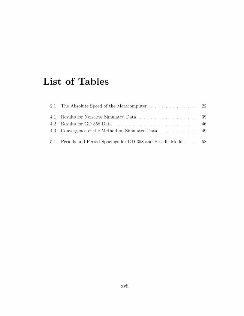
List of Tables
2.1 The Absolute Speed of the Metacomputer . . . . . . . . . . . . . 22
4.1 Results for Noiseless Simulated Data . . . . . . . . . . . . . . . . 39
4.2 Results for GD 358 Data . . . . . . . . . . . . . . . . . . . . . . . 46
4.3 Convergence of the Method on Simulated Data . . . . . . . . . . . 49
5.1 Periods and Period Spacings for GD 358 and Best-fit Models . . 58
xvii

xviii
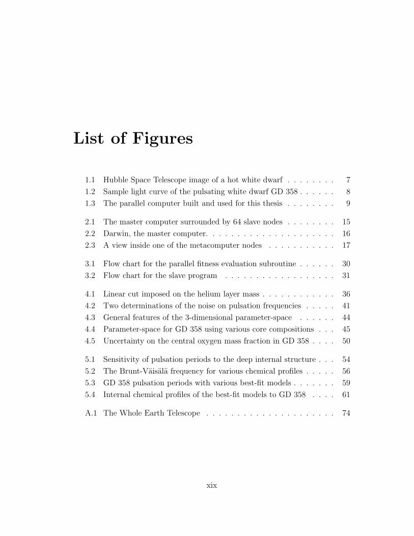
List of Figures
1.1 Hubble Space Telescope image of a hot white dwarf . . . . . . . . 7
1.2 Sample light curve of the pulsating white dwarf GD 358 . . . . . . 8
1.3 The parallel computer built and used for this thesis . . . . . . . . 9
2.1 The master computer surrounded by 64 slave nodes . . . . . . . . 15
2.2 Darwin, the master computer. . . . . . . . . . . . . . . . . . . . . 16
2.3 A view inside one of the metacomputer nodes . . . . . . . . . . . 17
3.1 Flow chart for the parallel fitness evaluation subroutine . . . . . . 30
3.2 Flow chart for the slave program . . . . . . . . . . . . . . . . . . 31
4.1 Linear cut imposed on the helium layer mass . . . . . . . . . . . . 36
4.2 Two determinations of the noise on pulsation frequencies . . . . . 41
4.3 General features of the 3-dimensional parameter-space . . . . . . 44
4.4 Parameter-space for GD 358 using various core compositions . . . 45
4.5 Uncertainty on the central oxygen mass fraction in GD 358 . . . . 50
5.1 Sensitivity of pulsation periods to the deep internal structure . . . 54
5.2 The Brunt-Vaisala frequency for various chemical profiles . . . . . 56
5.3 GD 358 pulsation periods with various best-fit models . . . . . . . 59
5.4 Internal chemical profiles of the best-fit models to GD 358 . . . . 61
A.1 The Whole Earth Telescope . . . . . . . . . . . . . . . . . . . . . 74
xix

xx
Chapter 1
Context
“In learning any subject of a technical nature where mathematics
plays a role...it is easy to confuse the proof itself with the relationship
it establishes. Clearly, the important thing to learn and to remember
is the relationship, not the proof.”
—Richard Feynman
1.1 Introduction
There isn’t much point in writing a dissertation if only a few people in the world
understand it, much less care enough about the subject to read every word. It
takes a long time to be educated as an astronomer, and by the time it’s over
most students have internalized the basic concepts. It’s easy to forget the mental
hurdles that challenged us along the way.
I began formal study in astronomy about ten years ago, and at every step
along the way my education has been subsidized by taxpayers. It seems only fair
that I should try to give something in return. I’ve decided to use the first chapter
of my dissertation to place my research project into a larger social context. I will
do my best to ensure that this chapter is comprehensible to the people who so
graciously and unknowingly helped me along the way. It’s the least I can do, and
maybe it will convince some of them that their investment was worthwhile.
1
2 CHAPTER 1. CONTEXT
1.2 What Good is Astronomy?
How can astronomers justify the support they receive from taxpayers? What
benefit does society derive from astronomical research? What is the rate of
return on their investment? These questions are difficult, but not impossible, to
answer. The economic benefits of basic scientific research are often realized over
the long-term, and it’s hard to anticipate what spin-offs may develop as a result
of any specific research program.
A purist might refuse even to respond to these questions. What justifica-
tion does basic research need other than the pursuit of knowledge? What higher
achievement can civilization hope to accomplish than the luxury of seeking an-
swers to some of the oldest questions: where did we come from, and what is our
place in the universe?
The proper response is probably somewhere in between. Over the years, ad-
vances in scientific knowledge made possible through basic research have had a
definite impact on the average citizen, but the magnitude of this impact is dif-
ficult to predict at the time the research is proposed. As a result, much of the
basic research funded by the public often sounds ridiculous to many taxpayers.
Gradually, this has led to a growing reluctance by the public to fund basic re-
search, and the annual budgets of government funding agencies have stagnated
as a consequence. Public education is an essential component of any strategy to
treat this problem effectively.
I contend that the money taxpayers contribute to scientific research in some
sense obligates the researchers to make their work accessible to the public. Some
combination of teaching and public outreach by researchers should provide an
adequate return on the investment. If this doesn’t seem reasonable, put it in
perspective by looking at exactly how much it costs U.S. taxpayers to fund as-
tronomical research:
• In the year 2000, the total federal budget amounted to $1.88 trillion1
• Revenue from personal income taxes amounted to $900 billion1
1http://w3.access.gpo.gov/usbudget/fy2000/table2 1.gif
1.3. THE NATURE OF KNOWLEDGE 3
• The “non-defense discretionary” portion of the budget totaled $330 billion2
• The National Science Foundation (NSF) budget was $3.95 billion3
• The NSF allocation to the Directorate for Mathematics & Physical Sciences
(MPS) amounted to $754 million4
• The MPS allocation to Astronomical Sciences amounted to $122 million4
So, even if you assume that the revenue for “non-defense discretionary” comes
entirely from personal income taxes, funding astronomy is cheap. Out of every
$1000 in revenue from personal income taxes, $365 goes into the non-defense dis-
cretionary fund. About $4.35 ends up in the hands of the National Science Foun-
dation. Of this, 83 cents goes to fund all of Mathematics & Physical Sciences.
In the end, for every $1000 in taxes only 13 cents ends up funding Astronomical
Sciences.
1.3 The Nature of Knowledge
Science is chiefly concerned with accumulating knowledge. What does this mean?
The Greek philosopher Plato defined knowledge as “justified true belief”. Belief
by itself is what we commonly call faith. There’s nothing wrong with faith, but
it doesn’t constitute knowledge under Plato’s definition. A belief that is justified
but false is simply a misconception. Based on incomplete information I may
be justified in believing that the Earth is flat, but I cannot know this to be so
because it turns out not to be true. Likewise, I may believe something that turns
out to be true even though I had no justification for believing it. For example, I
cannot know that a fair coin toss will turn up heads even if it does in fact turn
up heads, because I can have no defensible justification for this belief.
In science, our justification for believing something is usually based on ob-
servations of the world around us. The observations can occur either before or
2http://w3.access.gpo.gov/usbudget/fy2000/table2 2.gif3http://www.nsf.gov/bfa/bud/fy2000/overview.htm4http://www.nsf.gov/bfa/bud/fy2000/DirFund/mps.htm
4 CHAPTER 1. CONTEXT
after we have formulated a belief, corresponding to two broad methods of rea-
soning. In deductive reasoning, we begin by formulating a theory and deriving
specific hypothetical consequences that can be tested. We gather observations
to test the hypotheses and help to either confirm or refute the theory. In most
cases the match between observations and theory is imperfect, and we refine the
theory to try to account for the differences. Einstein’s theory of relativity is a
good example of this type of reasoning. Based on some reasonable fundamental
assumptions, Einstein developed a theory of the geometry of the universe. He
predicted some observational consequences of this theory and people tested these
predictions experimentally.
For inductive reasoning, we begin by looking for patterns in existing observa-
tions. We come up with some tentative hypotheses to explain the patterns, and
ultimately develop a general theory to explain the observed phenomena. Kepler’s
laws of planetary motion are good examples of inductive reasoning. Based on the
precise observations of the positions of planets in the night sky made by Tycho
Brahe, Kepler noticed some regular patterns. He developed several empirical
laws that helped us to understand the complex motions of the planets, which
ultimately inspired Newton to develop a general theory of gravity.
Armed with these methods of developing and justifying our beliefs, we slowly
converge on the truth. However, it’s important to realize that we may never
actually arrive at our goal. We may only be able to find better approximations
to the truth. In astronomy we do not have the luxury of designing the experiments
or manipulating the individual components, so knowledge in the strict sense is
even more difficult to obtain. Fortunately, the universe contains such a vast and
diverse array of phenomena that we have plenty to keep us occupied.
1.4 The Essence of my Dissertation Project
When I originally conceived of my dissertation project three years ago, the title
of my proposal was Genetic-Algorithm-based Optimization of White Dwarf Pul-
sation Models using an Intel/Linux Metacomputer. That’s quite a mouthful. It’s
actually much less intimidating than it sounds at first. Let me explain what this
project is really about, one piece at a time.
1.4. THE ESSENCE OF MY DISSERTATION PROJECT 5
1.4.1 Genetic Algorithms
Given the nature of knowledge, astronomers generally need to do two things to
learn anything useful about the universe. First, we need to gather quantitative
observations of something in the sky, usually with a telescope and some sophis-
ticated electronic detection equipment. Second, we need to interpret the obser-
vations by trying to match them with a mathematical model, using a computer.
The computer models have many different parameters—sort of like knobs and
switches that can be adjusted—and each represents some aspect of the physical
laws that govern the behavior of the model.
When we find a model that seems to match the observations fairly well, we
assume that the values of the parameters tell us something about the true nature
of the object we observed. The problem is: how do we know that some other
combination of parameters won’t do just as well, or even better, than the com-
bination we found? Or what if the model is simply inadequate to describe the
true nature of the object?
The process of adjusting the parameters to find a “best-fit” model to the
observations is essentially an optimization problem. There are many well estab-
lished mathematical tools (algorithms) for doing this—each with strengths and
weaknesses. I am using a relatively new approach that uses a process analogous
to Charles Darwin’s idea of evolution through natural selection. This so-called
genetic algorithm explores the many possible combinations of parameters, and
finds the best combination based on objective criteria.
1.4.2 White Dwarf Stars
What is a white dwarf star? To astronomers, dwarf is a general term for smaller
stars. The color of a star is an indication of the temperature at its surface. Very
hot objects emit more blue-white light, while cooler objects emit more red light.
Our Sun is termed a yellow dwarf and there are many stars cooler than the Sun
called red dwarfs. So a white dwarf is a relatively small star with a very hot
surface.
In 1844, an astronomer named Friedrich Bessel noticed that Sirius, the bright-
est star in the sky, appeared to wobble slightly as it moved through space. He
6 CHAPTER 1. CONTEXT
inferred that there must be something in orbit around it. Sure enough, in 1862
the faint companion was observed visually by Alvan Clark (a telescope maker)
and was given the name “Sirius B”. By the 1920’s, the companion had completed
one full orbit of Sirius and its mass was calculated, using Newton’s laws, to be
roughly the same as the Sun. When astronomers measured its spectrum, they
found that it emitted much more blue light than red, implying that it was very
hot on the surface even though it didn’t appear very bright in the sky. These
observations implied that it had to be a million times smaller than a regular star
with the same mass as the Sun—the first white dwarf!
The exact process of a star becoming a white dwarf depends on the mass of
the star, but all stars less massive than about 8 times the mass of the Sun (99% of
all stars) will eventually become white dwarfs. Normal stars fuse hydrogen into
helium until the hydrogen deep in the center begins to run out. For very massive
stars this may take only 1 million years—but for stars like the Sun the hydrogen
lasts for 10,000 million years. When enough helium collects in the middle of the
star, it becomes a significant source of extra heat. This messes up the internal
balance of the star, which then begins to bloat into a so-called red giant.
If the star is massive enough, it may eventually get hot enough in the center
to fuse the helium into carbon and oxygen. The star then enjoys another rel-
atively stable period, though much shorter this time. The carbon and oxygen,
in their turn, collect in the middle. If the star isn’t massive enough to reach
the temperature needed to fuse carbon and oxygen into heavier elements, then
these elements will simply continue to collect in the center until the helium fuel
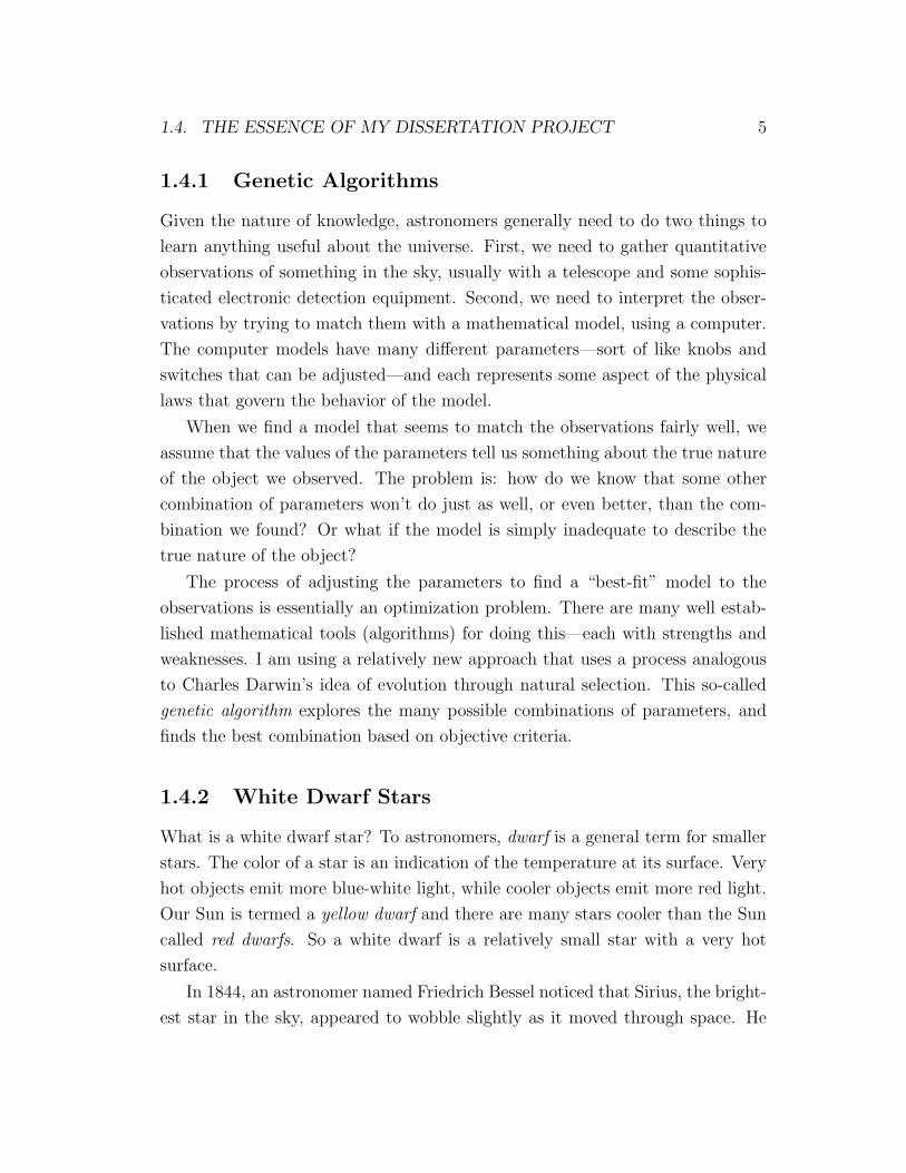
runs out. In the end, you have a carbon/oxygen white dwarf surrounded by the
remains of the original star (see Figure 1.1).
In normal stars like the Sun, the inward pull of gravity is balanced by the
outward push of the high-temperature material in the center, fusing hydrogen
into helium and releasing energy in the process. There is no nuclear fusion in a
white dwarf. Instead, the force that opposes gravity is called “electron degeneracy
pressure”.
When electrons are squeezed very close together, the energy-states that they
would normally be able to occupy become indistinguishable from the energy-
states of neighboring electrons. The rules of quantum mechanics tell us that
1.4. THE ESSENCE OF MY DISSERTATION PROJECT 7
Figure 1.1: A hot white dwarf at the center of the planetary nebula NGC 2440.This image was obtained with the Hubble Space Telescope by H. Bond (STScI)and R. Ciardullo (PSU).
no two electrons can occupy exactly the same energy-state, and as the average
distance between electrons gets smaller the average momentum must get larger.
So, the electrons are forced into higher energy-states (pushed to higher speeds)
just because of the density of the matter.
This quantum pressure can oppose gravity as long as the density doesn’t
get too high. If a white dwarf has more than about 1.4 times the mass of the
Sun squeezing the material, there will be too few energy-states available to the
electrons (since they cannot travel faster than the speed of light) and the star
will collapse—causing a supernova explosion.
Pulsating White Dwarfs
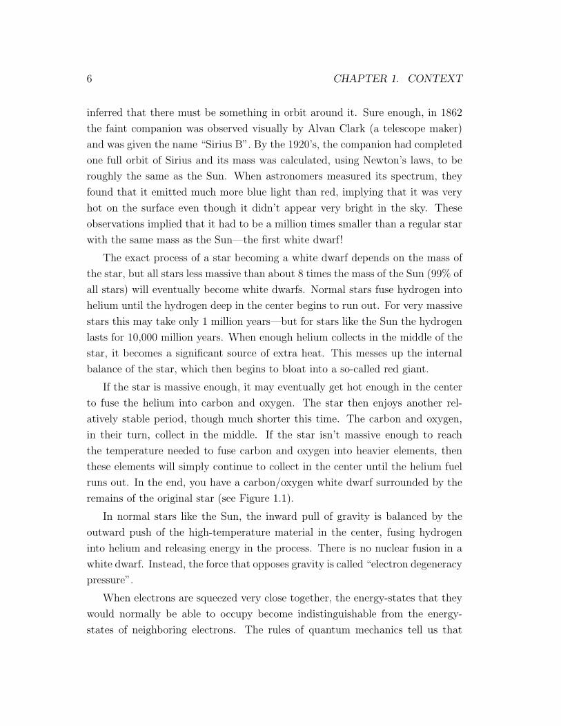
Some white dwarfs show very regular variations in the amount of light reaching
our telescopes (see Figure 1.2). The pattern of this variation suggests that these
white dwarfs are pulsating—as if there are continuous star-quakes going on. By
studying the patterns of light variation, astronomers can learn about the interior
structure of white dwarfs—in much the same way as seismologists can learn about
the inside of the Earth by studying earthquakes. For this reason, the study of
8 CHAPTER 1. CONTEXT
Figure 1.2: Non-radial pulsations in some white dwarf stars cause periodicchanges in their brightness over time. This sample light curve of GD 358 showsmany pulsation periods excited simultaneously, causing beating and a total vari-ation of about 10 percent on timescales shorter than an hour.
these pulsating white dwarfs is called asteroseismology.
Since 1988, very useful observations of pulsating white dwarfs have been ob-
tained with the Whole Earth Telescope—a collaboration of astronomers around
the globe who cooperate to monitor these stars for weeks at a time. I have helped
to make some of these observations, but I have also worked on interpreting them
using our computer models. I have approached the models in two ways:
• I assume the models are accurate representations of the real white dwarf
stars, and I try to find the combination of model parameters that do the
best job of matching the observations.
• I assume the models are incomplete representations of the real white dwarf
stars, and I try to find changes to the internal structure of the models that
yield an improved match to the observations.
1.4.3 Linux Metacomputer
The dictionary definition of the prefix meta- is: “Beyond; More comprehensive;
More highly developed.” So a meta-computer goes beyond the boundaries of a
1.4. THE ESSENCE OF MY DISSERTATION PROJECT 9
traditional computer as we are accustomed to thinking of it. Essentially, a meta-
computer is a collection of many individual computers, connected by a network
(the Internet for example), which can cooperate on solving a problem. In general,
this allows the problem to be solved much more quickly than would be possible
using a single computer.
Supercomputers are much faster than a single desktop computer too, but
they usually cost millions of dollars, and everyone has to compete for time to
work on their problem. Recently, personal computers have become very fast and
relatively inexpensive. At the same time, the idea of free software (like the Linux
operating system) has started to catch on. These developments have made it
feasible to build a specialized metacomputer with as much computing power as
a 5-year-old supercomputer, but for only about 1% of the cost!
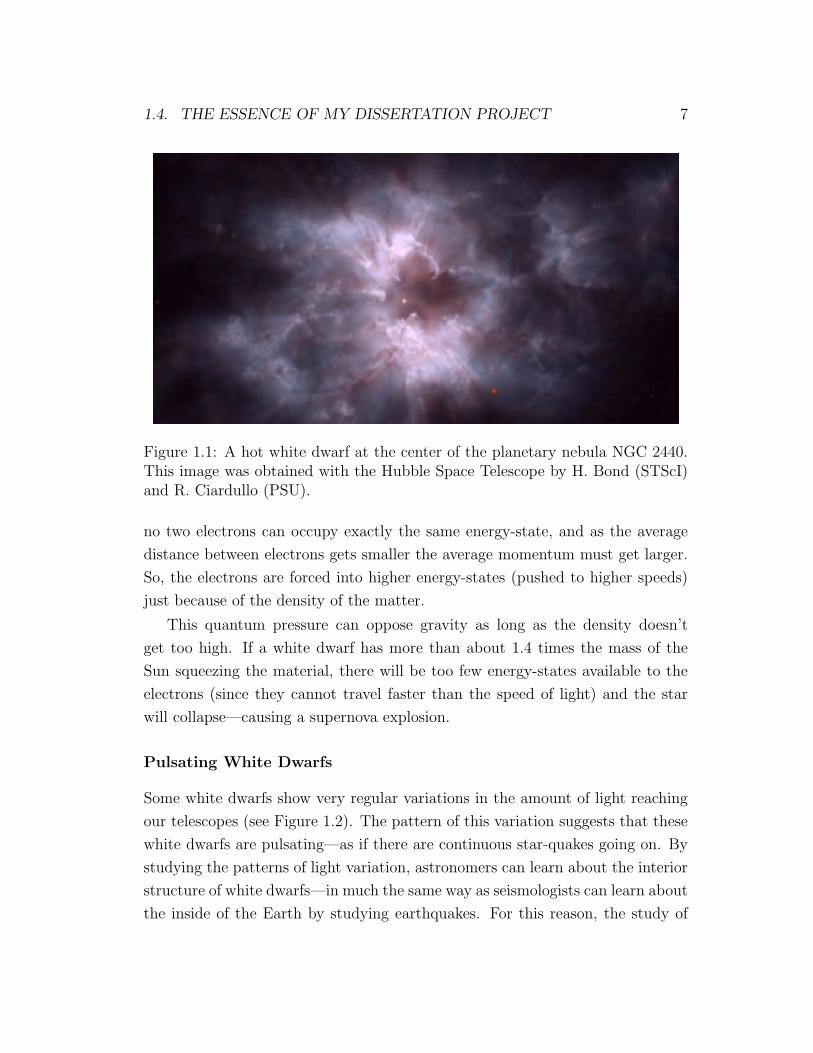
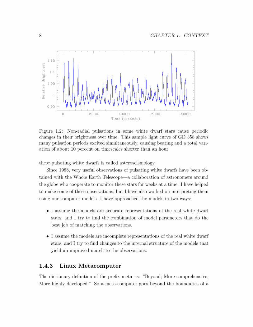
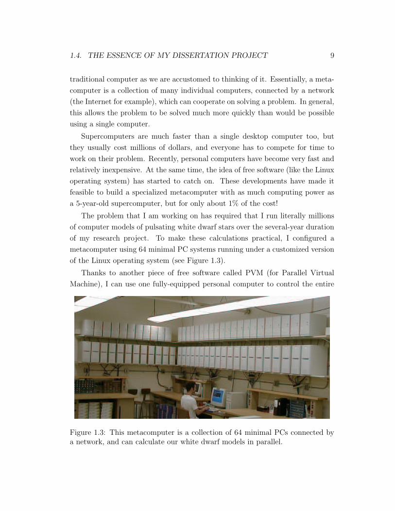
The problem that I am working on has required that I run literally millions
of computer models of pulsating white dwarf stars over the several-year duration
of my research project. To make these calculations practical, I configured a
metacomputer using 64 minimal PC systems running under a customized version
of the Linux operating system (see Figure 1.3).
Thanks to another piece of free software called PVM (for Parallel Virtual
Machine), I can use one fully-equipped personal computer to control the entire
Figure 1.3: This metacomputer is a collection of 64 minimal PCs connected bya network, and can calculate our white dwarf models in parallel.
10 CHAPTER 1. CONTEXT
system. This central computer is responsible for distributing work to each of
the 64 processors, and collecting the results. There is a small amount of work
required just to keep track of everything, so the metacomputer actually runs
about 60 (rather than 64) times as fast as a single system. Not bad!
1.4.4 The Big Picture
So I’m using a relatively new optimization method to find the best set of pa-
rameters to match the observations with our computer models of pulsating white
dwarf stars; and there are so many models to run that I need a lot of computing
power, so I linked a bunch of PC systems together to do the job. But what do I
hope to learn?
Well, the source of energy for regular stars like the Sun is nuclear fusion. This
is the kind of nuclear energy that doesn’t produce any dangerous radioactive
waste. Astronomers have a good idea of how fusion energy works to power stars,
but the process requires extremely high temperatures and pressures, which must
be sustained for a long time; these conditions are difficult to reproduce (in a
controlled way) in laboratories on Earth. Physicists have been working on it for
several decades, but sustained nuclear fusion has still never been achieved. This
leads us to believe that we may not understand all of the physics that we need to
make fusion work. If scientists could learn to achieve controlled nuclear fusion,
it would provide an essentially inexhaustible source of clean, sustainable energy.
To help ensure that we properly understand how stars work, it is useful to look
at the “ashes” of the nuclear fusion. Those ashes are locked in the white dwarf
stars, and asteroseismology allows us to peer down inside and probe around. But
our understanding can only be as good as our models, so it is important both
to make sure that we find the absolute “best” match, and to figure out what
limitations are imposed simply by using the models we use. It’s only one piece
of the puzzle, but it’s a place to start.
1.5 Organization of this Dissertation
Most of the work presented in this dissertation has already been published. Each
chapter should be able to stand by itself, and together they tell the story of how
1.5. ORGANIZATION OF THIS DISSERTATION 11
I’ve spent the last three years of my professional life.
Chapter 2 describes the development of the Linux metacomputer and provides
a detailed account of its inner workings. The text is derived from articles pub-
lished in the Linux Journal, Baltic Astronomy, and a Metacomputer mini-howto
posted on the world-wide web.
Chapter 3 includes a more detailed background on genetic algorithms. I out-
line the steps I took to create a parallel version of a general-purpose genetic
algorithm in the public domain, and its implementation on the Linux metacom-
puter.
Chapter 4 is derived primarily from a paper published in the Astrophysical
Journal in December 2000. It describes the first application of the genetic algo-
rithm approach to model pulsations in the white dwarf GD 358, and an extension
of the method to determine its internal composition and structure.
Chapter 5 comes from a paper published in the Astrophysical Journal in Au-
gust 2001. It describes a method of “reverse engineering” the internal structure
of a pulsating white dwarf by using the genetic algorithm and the models in a
slightly different way.
Chapter 6 sums up the major conclusions of this work and outlines future
directions. The appendices contain an archive of my observations for the Whole
Earth Telescope, some interactive simulations of pulsating white dwarfs, and an
archive of the computer codes used for this dissertation.

12 CHAPTER 1. CONTEXT
Chapter 2
Linux Metacomputer
“There’s certainly a strong case for people disliking Microsoft because
their operating systems... suck.”
—Linus Torvalds
2.1 Introduction
The adjustable parameters in our computer models of white dwarfs presently
include the total mass, the temperature, hydrogen and helium layer masses,
core composition, convective efficiency, and internal chemical profiles. Finding
a proper set of these to provide a close fit to the observed data is difficult.
The traditional procedure is a guess-and-check process guided by intuition and
experience, and is far more subjective than we would like. Objective proce-
dures for determining the best-fit model are essential if asteroseismology is to
become a widely-accepted and reliable astronomical technique. We must be able
to demonstrate that for a given model, within the range of different values the
model parameters can assume, we have found the only solution, or the best one
if more than one is possible. To address this problem, we have applied a search-
and-fit technique employing a genetic algorithm (GA), which can explore the
myriad parameter combinations possible and select for us the best one, or ones
(cf. Goldberg, 1989; Charbonneau, 1995; Metcalfe, 1999).
13
14 CHAPTER 2. LINUX METACOMPUTER
2.2 Motivation
Although genetic algorithms are often more efficient than other global techniques,
they are still quite demanding computationally. On a reasonably fast computer,
it takes about a minute to calculate the pulsation periods of a single white dwarf
model. However, finding the best-fit with the GA method requires the evaluation
of hundreds of thousands of such models. On a single computer, it would take
more than two months to find an answer. To develop this method on a reasonable
timescale, we realized that we would need our own parallel computer.
It was January 1998, and the idea of parallel computing using inexpensive
personal computer (PC) hardware and the free Linux operating system started
getting a lot of attention. The basic idea was to connect a bunch of PCs together
on a network, and then to split up the computing workload and use the machines
collectively to solve the problem more quickly. Such a machine is known to
computer scientists as a metacomputer. This differs from a supercomputer, which
is much more expensive since all of the computing power is integrated into a
single unified piece of hardware.
There are several advantages to using a metacomputer rather than a more
traditional supercomputer. The primary advantage is price: a metacomputer
that is just as fast as a 5-year-old supercomputer can be built for only about
1 percent of the cost—about $10,000 rather than $1 million! Another major
advantage is access: the owner and administrator of a parallel computer doesn’t
need to compete with other researchers for time or resources, and the hardware
and software configuration can be optimized for a specific problem. Finally if
something breaks, replacement parts are standard off-the-shelf components that
are widely available, and while they are on order the computer is still functional
at a slightly reduced capacity.
2.3 Hardware
The first Linux metacomputer, known as the Beowulf cluster5 (Becker et al.,
1995), has now become the prototype for many general-purpose Linux clusters.
5http://www.beowulf.org/
2.3. HARDWARE 15
Our machine is similar to Beowulf in the sense that it consists of many indepen-
dent PCs, or nodes; but our goal was to design a special-purpose computational
tool with the best performance possible per dollar, so our machine differs from
Beowulf in several important ways.
We wanted to use each node of the metacomputer to run identical tasks (white
dwarf pulsation models) with small, independent sets of data (the parameters for
each model). The results of the calculations performed by the nodes consisted
of just a few numbers (the root-mean-square differences between the observed
and calculated pulsation periods) which only needed to be communicated to
the master process (the genetic algorithm), never to another node. Essentially,
network bandwidth was not an issue because the computation to communication
ratio of our application was extremely high, and hard disks were not needed on
the nodes because our problem did not require any significant amount of data
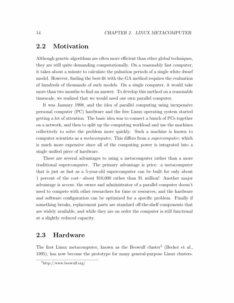
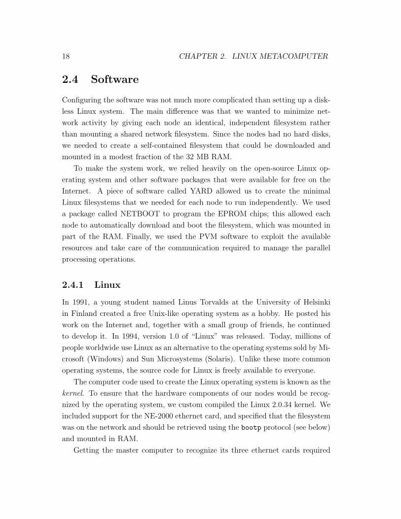
storage. We settled on a design including one master computer and 64 minimal
nodes connected by a simple coaxial network (see Figure 2.1).
We developed the metacomputer in four phases. To demonstrate that we
could make the system work, we started with the master computer and only two
nodes. When the first phase was operational, we expanded it to a dozen nodes to
Figure 2.1: The 64 minimal nodes of the metacomputer on shelves surroundingthe master computer.
16 CHAPTER 2. LINUX METACOMPUTER
demonstrate that the performance would scale. In the third phase, we occupied
the entire bottom shelf with a total of 32 nodes. Months later, we were given
the opportunity to expand the system by an additional 32 nodes with processors
donated by AMD and we filled the top shelf, yielding a total of 64 nodes.
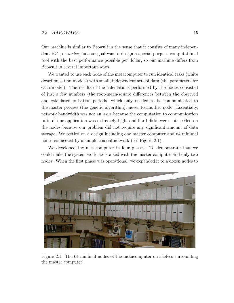
2.3.1 Master Computer
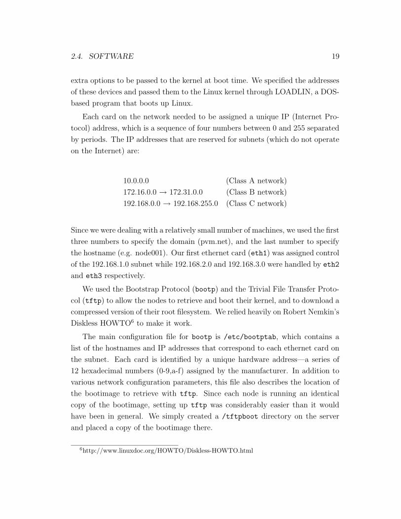
Our master computer, which we call Darwin, is a Pentium-II 333 MHz system
with 128 MB RAM and two 8.4 GB hard disks (see Figure 2.2). It has three NE-
2000 compatible network cards, each of which drives 1/3 of the nodes on a subnet.
No more than 30 devices (e.g. ethernet cards in the nodes) can be included on a
single subnet without using a repeater to boost the signal. Additional ethernet
cards for the master computer were significantly less expensive than a repeater.
Figure 2.2: Darwin, the master computer controlling all 64 nodes.
2.3. HARDWARE 17
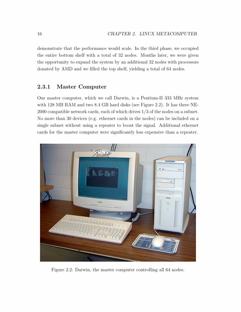
2.3.2 Slave Nodes
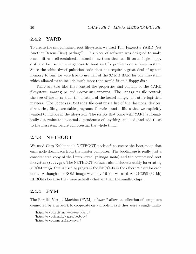
We assembled the nodes from components obtained at a local discount computer
outlet. Each node includes only an ATX tower case and power supply with a
motherboard, a processor and fan, a single 32 MB RAM chip, and an NE-2000
compatible network card (see Figure 2.3). Half of the nodes contain Pentium-II
300 MHz processors, while the other half are AMD K6-II 450 MHz chips. We
added inexpensive Am27C256 32 kb EPROMs (erasable programmable read-only
memory) to the bootrom sockets of each network card. The nodes are connected
in series with 3-ft ethernet coaxial cables, and the subnets have 50 Ω terminators
on each end. The total cost of the system was around $25,000 but it could be
built for considerably less today, and less still tomorrow.
Figure 2.3: A view inside one of the metacomputer nodes.
18 CHAPTER 2. LINUX METACOMPUTER
2.4 Software
Configuring the software was not much more complicated than setting up a disk-
less Linux system. The main difference was that we wanted to minimize net-
work activity by giving each node an identical, independent filesystem rather
than mounting a shared network filesystem. Since the nodes had no hard disks,
we needed to create a self-contained filesystem that could be downloaded and
mounted in a modest fraction of the 32 MB RAM.
To make the system work, we relied heavily on the open-source Linux op-
erating system and other software packages that were available for free on the
Internet. A piece of software called YARD allowed us to create the minimal
Linux filesystems that we needed for each node to run independently. We used
a package called NETBOOT to program the EPROM chips; this allowed each
node to automatically download and boot the filesystem, which was mounted in
part of the RAM. Finally, we used the PVM software to exploit the available
resources and take care of the communication required to manage the parallel
processing operations.
2.4.1 Linux
In 1991, a young student named Linus Torvalds at the University of Helsinki
in Finland created a free Unix-like operating system as a hobby. He posted his
work on the Internet and, together with a small group of friends, he continued
to develop it. In 1994, version 1.0 of “Linux” was released. Today, millions of
people worldwide use Linux as an alternative to the operating systems sold by Mi-
crosoft (Windows) and Sun Microsystems (Solaris). Unlike these more common
operating systems, the source code for Linux is freely available to everyone.
The computer code used to create the Linux operating system is known as the
kernel. To ensure that the hardware components of our nodes would be recog-
nized by the operating system, we custom compiled the Linux 2.0.34 kernel. We
included support for the NE-2000 ethernet card, and specified that the filesystem
was on the network and should be retrieved using the bootp protocol (see below)
and mounted in RAM.
Getting the master computer to recognize its three ethernet cards required
2.4. SOFTWARE 19
extra options to be passed to the kernel at boot time. We specified the addresses
of these devices and passed them to the Linux kernel through LOADLIN, a DOS-
based program that boots up Linux.
Each card on the network needed to be assigned a unique IP (Internet Pro-
tocol) address, which is a sequence of four numbers between 0 and 255 separated
by periods. The IP addresses that are reserved for subnets (which do not operate
on the Internet) are:
10.0.0.0 (Class A network)
172.16.0.0 → 172.31.0.0 (Class B network)
192.168.0.0 → 192.168.255.0 (Class C network)
Since we were dealing with a relatively small number of machines, we used the first
three numbers to specify the domain (pvm.net), and the last number to specify
the hostname (e.g. node001). Our first ethernet card (eth1) was assigned control
of the 192.168.1.0 subnet while 192.168.2.0 and 192.168.3.0 were handled by eth2
and eth3 respectively.
We used the Bootstrap Protocol (bootp) and the Trivial File Transfer Proto-
col (tftp) to allow the nodes to retrieve and boot their kernel, and to download a
compressed version of their root filesystem. We relied heavily on Robert Nemkin’s
Diskless HOWTO6 to make it work.
The main configuration file for bootp is /etc/bootptab, which contains a
list of the hostnames and IP addresses that correspond to each ethernet card on
the subnet. Each card is identified by a unique hardware address—a series of
12 hexadecimal numbers (0-9,a-f) assigned by the manufacturer. In addition to
various network configuration parameters, this file also describes the location of
the bootimage to retrieve with tftp. Since each node is running an identical
copy of the bootimage, setting up tftp was considerably easier than it would
have been in general. We simply created a /tftpboot directory on the server
and placed a copy of the bootimage there.
6http://www.linuxdoc.org/HOWTO/Diskless-HOWTO.html
20 CHAPTER 2. LINUX METACOMPUTER
2.4.2 YARD
To create the self-contained root filesystem, we used Tom Fawcett’s YARD (Yet
Another Rescue Disk) package7. This piece of software was designed to make
rescue disks—self-contained minimal filesystems that can fit on a single floppy
disk and be used in emergencies to boot and fix problems on a Linux system.
Since the white dwarf pulsation code does not require a great deal of system
memory to run, we were free to use half of the 32 MB RAM for our filesystem,
which allowed us to include much more than would fit on a floppy disk.
There are two files that control the properties and content of the YARD
filesystem: Config.pl and Bootdisk Contents. The Config.pl file controls
the size of the filesystem, the location of the kernel image, and other logistical
matters. The Bootdisk Contents file contains a list of the daemons, devices,
directories, files, executable programs, libraries, and utilities that we explicitly
wanted to include in the filesystem. The scripts that come with YARD automat-
ically determine the external dependences of anything included, and add those
to the filesystem before compressing the whole thing.
2.4.3 NETBOOT
We used Gero Kuhlmann’s NETBOOT package8 to create the bootimage that
each node downloads from the master computer. The bootimage is really just a
concatenated copy of the Linux kernel (zImage.node) and the compressed root
filesystem (root.gz). The NETBOOT software also includes a utility for creating
a ROM image that is used to program the EPROMs in the ethernet card for each
node. Although our ROM image was only 16 kb, we used Am27C256 (32 kb)
EPROMs because they were actually cheaper than the smaller chips.
2.4.4 PVM
The Parallel Virtual Machine (PVM) software9 allows a collection of computers
connected by a network to cooperate on a problem as if they were a single multi-
7http://www.croftj.net/∼fawcett/yard/8http://www.han.de/∼gero/netboot/9http://www.epm.ornl.gov/pvm/
2.5. HOW IT WORKS 21
processor parallel machine. It was developed in the 1990’s at Oak Ridge National
Laboratory (Geist et al., 1994). The software consists of a daemon running
on each host in the virtual machine, and a library of routines that need to be
incorporated into a computer program so that it can utilize all of the available
computing power.
2.5 How it works
With the master computer up and running, we turn on one node at a time
(to prevent the server from being overwhelmed by many simultaneous bootp
requests). By default, the node tries to boot from the network first. It finds the
bootrom on the ethernet card, and executes the ROM program. This program
initializes the ethernet card and broadcasts a bootp request over the network.
When the server receives the request, it identifies the unique hardware ad-
dress, assigns the corresponding IP address from the /etc/bootptab file, and
allows the requesting node to download the bootimage. The node loads the
Linux kernel image into memory, creates a 16 MB initial ramdisk, mounts the
root filesystem, and starts all essential services and daemons.
Once all of the nodes are up, we start the PVM daemons on each node from
the master computer. Any computer program that incorporates the PVM library
routines and has been included in the root filesystem can then be run in parallel.
2.6 Benchmarks
Measuring the absolute performance of the metacomputer is difficult because
the result strongly depends on the fraction of Floating-point Division operations
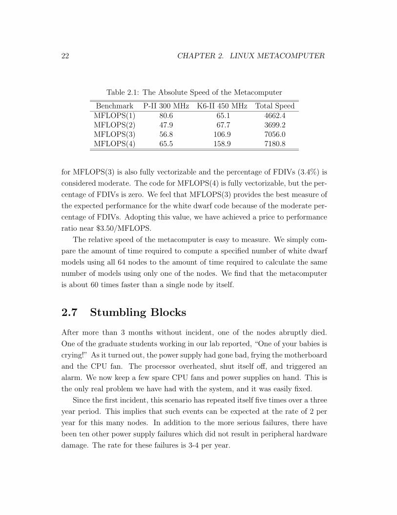
(FDIVs) used in the benchmark code. Table 2.1 lists four different measures of the
absolute speed in Millions of FLoating-point Operations Per Second (MFLOPS).
The code for MFLOPS(1) is essentially scalar, which means that it cannot
exploit any advantages that are intrinsic to processor instruction sets; the per-
centage of FDIVs (9.6%) is considered somewhat high. The code for MFLOPS(2)
is fully vectorizable, which means that it can exploit advantages intrinsic to each
processor, but the percentage of FDIVs (9.2%) is still on the high side. The code
22 CHAPTER 2. LINUX METACOMPUTER
Table 2.1: The Absolute Speed of the Metacomputer
Benchmark P-II 300 MHz K6-II 450 MHz Total SpeedMFLOPS(1) 80.6 65.1 4662.4MFLOPS(2) 47.9 67.7 3699.2MFLOPS(3) 56.8 106.9 7056.0MFLOPS(4) 65.5 158.9 7180.8
for MFLOPS(3) is also fully vectorizable and the percentage of FDIVs (3.4%) is
considered moderate. The code for MFLOPS(4) is fully vectorizable, but the per-
centage of FDIVs is zero. We feel that MFLOPS(3) provides the best measure of
the expected performance for the white dwarf code because of the moderate per-
centage of FDIVs. Adopting this value, we have achieved a price to performance
ratio near $3.50/MFLOPS.
The relative speed of the metacomputer is easy to measure. We simply com-
pare the amount of time required to compute a specified number of white dwarf
models using all 64 nodes to the amount of time required to calculate the same
number of models using only one of the nodes. We find that the metacomputer
is about 60 times faster than a single node by itself.
2.7 Stumbling Blocks
After more than 3 months without incident, one of the nodes abruptly died.
One of the graduate students working in our lab reported, “One of your babies is
crying!” As it turned out, the power supply had gone bad, frying the motherboard
and the CPU fan. The processor overheated, shut itself off, and triggered an
alarm. We now keep a few spare CPU fans and power supplies on hand. This is
the only real problem we have had with the system, and it was easily fixed.
Since the first incident, this scenario has repeated itself five times over a three
year period. This implies that such events can be expected at the rate of 2 per
year for this many nodes. In addition to the more serious failures, there have
been ten other power supply failures which did not result in peripheral hardware
damage. The rate for these failures is 3-4 per year.
Chapter 3
Parallel Genetic Algorithm
“Evolution is cleverer than you are.”
—Francis Crick
3.1 Background
The problem of extracting useful information from a set of observational data
often reduces to finding the set of parameters for some theoretical model which
results in the closest match to the observations. If the physical basis of the
model is both accurate and complete, then the values of the parameters for the
best-fit model can yield important insights into the nature of the object under
investigation.
When searching for the best-fit set of parameters, the most fundamental con-
sideration is: where to begin? Models of all but the simplest physical systems are
typically non-linear, so finding the least-squares fit to the data requires an initial
guess for each parameter. Generally, some iterative procedure is used to im-
prove upon this first guess in order to find the model with the absolute minimum
residuals in the multi-dimensional parameter-space.
There are at least two potential problems with this standard approach to
model fitting. The initial set of parameters is typically determined by drawing
upon the past experience of the person who is fitting the model. This subjective
method is particularly disturbing when combined with a local approach to iter-
23
24 CHAPTER 3. PARALLEL GENETIC ALGORITHM
ative improvement. Many optimization schemes, such as differential corrections
(Proctor & Linnell, 1972) or the simplex method (Kallrath & Linnell, 1987),
yield final results which depend to some extent on the initial guesses. The con-
sequences of this sort of behavior are not serious if the parameter-space is well
behaved—that is, if it contains a single, well defined minimum. If the parameter-
space contains many local minima, then it can be more difficult for the traditional
approach to find the global minimum.
3.2 Genetic Algorithms
An optimization scheme based on a genetic algorithm (GA) can avoid the prob-
lems inherent in more traditional approaches. Restrictions on the range of the
parameter-space are imposed only by observations and by the physics of the
model. Although the parameter-space so-defined is often quite large, the GA
provides a relatively efficient means of searching globally for the best-fit model.
While it is difficult for GAs to find precise values for the set of best-fit parame-
ters, they are well suited to search for the region of parameter-space that contains
the global minimum. In this sense, the GA is an objective means of obtaining a
good first guess for a more traditional method which can narrow in on the precise
values and uncertainties of the best-fit.
The underlying ideas for genetic algorithms were inspired by Charles Darwin’s
(1859) notion of biological evolution through natural selection. The basic idea
is to solve an optimization problem by evolving the best solution from an initial
set of completely random guesses. The theoretical model provides the framework
within which the evolution takes place, and the individual parameters control-
ling it serve as the genetic building blocks. Observations provide the selection
pressure. A comprehensive description of how to incorporate these ideas in a
computational setting was written by Goldberg (1989).
Initially, the parameter-space is filled uniformly with trials consisting of ran-
domly chosen values for each parameter, within a range based on the physics
that the parameter is supposed to describe. The model is evaluated for each
trial, and the result is compared to the observed data and assigned a fitness
based on the relative quality of the match. A new generation of trials is then
3.2. GENETIC ALGORITHMS 25
created by selecting from this population at random, weighted by the fitness.
To apply genetic operations to the new generation of trials, their characteris-
tics must be encoded in some manner. The most straightforward way of encoding
them is to convert the numerical values of the parameters into a long string of
numbers. This string is analogous to a chromosome, and each number represents
a gene. For example, a two parameter trial with numerical values x1 = 1.234 and
y1 = 5.678 would be encoded into a single string of numbers ‘12345678’.
Next, the encoded trials are paired up and modified in order to explore new
regions of parameter-space. Without this step, the final solution could ultimately
be no better than the single best trial contained in the initial population. The two
basic operations are crossover which emulates sexual reproduction, and mutation
which emulates happenstance and cosmic rays.
As an example, suppose that the encoded trial above is paired up with another
trial having x2 = 2.468 and y2 = 3.579, which encodes to the string ‘24683579’.
The crossover procedure chooses a random position between two numbers along
the string, and swaps the two strings from that position to the end. So if the
third position is chosen, the strings become
123|45678→ 123|83579
246|83579→ 246|45678
Although there is a high probability of crossover, this operation is not applied to
all of the pairs. This helps to keep favorable characteristics from being eliminated
or corrupted too hastily. To this same end, the rate of mutation is assigned a
relatively low probability. This operation allows for the spontaneous transforma-
tion of any particular position on the string into a new randomly chosen value.
So if the mutation operation were applied to the sixth position of the second
trial, the result might be
24645|6|78→ 24645|0|78
After these operations have been applied, the strings are decoded back into
sets of numerical values for the parameters. In this example, the new first
string ‘12383579’ becomes x1 = 1.238 and y1 = 3.579 and the new second string
‘24645078’ becomes x2 = 2.464 and y2 = 5.078. This new generation replaces
26 CHAPTER 3. PARALLEL GENETIC ALGORITHM
the old one, and the process begins again. The evolution continues until one
region of parameter-space remains populated while other regions become essen-
tially empty. The robustness of the solution can be established by running the
GA several times with different random initialization.
Genetic algorithms have been used a great deal for optimization problems in
other fields, but until recently they have not attracted much attention in astron-
omy. The application of GAs to problems of astronomical interest was promoted
by Charbonneau (1995), who demonstrated the technique by fitting the rotation
curves of galaxies, a multiply-periodic signal, and a magneto-hydrodynamic wind
model. Many other applications of GAs to astronomical problems have appeared
in the recent literature. Hakala (1995) optimized the accretion stream map of
an eclipsing polar. Lang (1995) developed an optimum set of image selection
criteria for detecting high-energy gamma rays. Kennelly et al. (1995) used radial
velocity observations to identify the oscillation modes of a δ Scuti star. Lazio
(1997) searched pulsar timing signals for the signatures of planetary companions.
Charbonneau et al. (1998) performed a helioseismic inversion to constrain solar
core rotation. Wahde (1998) determined the orbital parameters of interacting
galaxies. Metcalfe (1999) used a GA to fit the light curves of an eclipsing binary
star. The applicability of GAs to such a wide range of astronomical problems is
a testament to their versatility.
3.3 Parallelizing PIKAIA
There are only two ways to make a computer program run faster—either make
the code more efficient, or run it on a faster machine. We made a few design
improvements to the original white dwarf code, but they decreased the runtime
by only ∼10%. We decided that we really needed access to a faster machine. We
looked into the supercomputing facilities available through the university, but
the idea of using a supercomputer didn’t appeal to us very much; the process
seemed to involve a great deal of red tape, and we weren’t certain that we could
justify time on a supercomputer in any case. To be practical, the GA-based fit-
ting technique required a dedicated instrument to perform the calculations. We
designed and configured such an instrument—an isolated network of 64 minimal
3.3. PARALLELIZING PIKAIA 27
PCs running Linux (Metcalfe & Nather, 1999, 2000). To allow the white dwarf
code to be run on this metacomputer, we incorporated the message passing rou-
tines of the Parallel Virtual Machine (PVM) software into the public-domain
genetic algorithm PIKAIA.
3.3.1 Parallel Virtual Machine
The PVM software (Geist et al., 1994) allows a collection of networked comput-
ers to cooperate on a problem as if they were a single multi-processor parallel
machine. All of the software and documentation was free. We had no trouble
installing it, and the sample programs that came with the distribution made it
easy to learn how to use. The trickiest part of the whole procedure was figuring
out how to split up the workload among the various computers.
The GA-based fitting procedure for the white dwarf code quite naturally
divided into two basic functions: evolving and pulsating white dwarf models,
and manipulating the results from each generation of trials. When we profiled
the distribution of execution time for each part of the code, this division became
even more obvious. The majority of the computing time was spent evolving the
starter model to a specific temperature. The GA is concerned only with collecting
and organizing the results of many of these models, so it seemed reasonable to
allocate many slave computers to carry out the model calculations while a master
computer took care of the GA-related tasks.
In addition to decomposing the function of the code, a further division based
on the data was also possible. Since there were many trials in each generation,
the data required by the GA could easily be split into small, computationally
manageable units. One model could be sent to each available slave computer,
so the number of machines available would control the number of models which
could be calculated at the same time.
One minor caveat to the decomposition of the data into separate models to be
calculated by different computers is the fact that half of the machines are slightly
faster than the other half. Much of the potential increase in efficiency from this
parallelizing scheme could be lost if fast machines are not sent more models to
compute than slow ones. This may seem trivial, but there is no mechanism
28 CHAPTER 3. PARALLEL GENETIC ALGORITHM
built in to the current version of the PVM software to handle this procedure
automatically.
It is also potentially problematic to send out new jobs only after receiving the
results of previous jobs because the computers sometimes hang or crash. Again,
this may seem obvious—but unless specifically asked to check, PVM cannot tell
the difference between a crashed computer and one that simply takes a long time
to compute a model. At the end of a generation of trials, if the master process
has not received the results from one of the slave jobs, it would normally just
continue to wait for the response indefinitely.
3.3.2 The PIKAIA Subroutine
PIKAIA is a self-contained, genetic-algorithm-based optimization subroutine de-
veloped by Paul Charbonneau and Barry Knapp at the High Altitude Obser-
vatory in Boulder, Colorado. Most optimization techniques work to minimize
a quantity—like the root-mean-square (r.m.s.) residuals; but it is more natural
for a genetic algorithm to maximize a quantity—natural selection works through
survival of the fittest. So PIKAIA maximizes a specified FORTRAN function
through a call in the body of the main program.
Unlike many GA packages available commercially or in the public domain,
PIKAIA uses decimal (rather than binary) encoding. Binary operations are
usually carried out through platform-dependent functions in FORTRAN, which
makes it more difficult to port the code between the Intel and Sun platforms.
PIKAIA incorporates only the two basic genetic operators: uniform one-point
crossover, and uniform one-point mutation. The mutation rate can be dynami-
cally adjusted during the evolution, using either the linear distance in parameter-
space or the difference in fitness between the best and median solutions in the
population. The practice of keeping the best solution from each generation is
called elitism, and is a default option in PIKAIA. Selection is based on ranking
rather than absolute fitness, and makes use of the Roulette Wheel algorithm.
There are three different reproduction plans available in PIKAIA: Steady-State-
Delete-Random, Steady-State-Delete-Worst, and Full Generational Replacement.
Only the last of these is easily parallelizable.
3.4. MASTER PROGRAM 29
3.4 Master Program
Starting with an improved unreleased version of PIKAIA, we incorporated themessage passing routines of PVM into a parallel fitness evaluation subroutine.The original code evaluated the fitnesses of the population of trials one at a timein a DO loop. We replaced this procedure with a single call to a new subroutinethat evaluates the fitnesses in parallel on all available processors.
c initialize (random) phenotypes
do ip=1,np
do k=1,n
oldph(k,ip)=urand()
enddo
c calculate fitesses
c fitns(ip) = ff(n,oldph(1,ip))
enddo
c calculate fitnesses in parallel
call pvm_fitness(’ff_slave’, np, n, oldph, fitns)
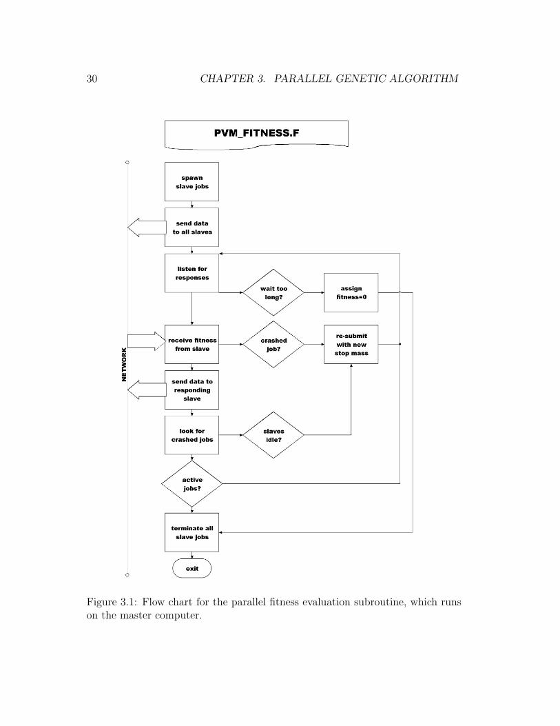
The parallel version of PIKAIA constitutes the master program which runs on
Darwin, the central computer in the network. A full listing of the parallel fitness
evaluation subroutine (PVM FITNESS.F) is included in Appendix C. A flow
chart for this code is shown in Figure 3.1.
After starting the slave program on every available processor (64 for our
metacomputer), PVM FITNESS.F sends an array containing the values of the
parameters to each slave job over the network. In the first generation of the
GA, these values are completely random; in subsequent generations, they are the
result of the selection and mutation of the previous generation, performed by the
non-parallel portions of PIKAIA.
Next, the subroutine listens for responses from the network and sends a new
set of parameters to each slave job as it finishes the previous calculation. When
all sets of parameters have been sent out, the subroutine begins looking for jobs
that seem to have crashed and re-submits them to slaves that have finished and
would otherwise sit idle. If a few jobs do not return a fitness after about five
times the average runtime required to compute a model, the subroutine assigns
them a fitness of zero. When every set of parameters in the generation have been
assigned a fitness value, the subroutine returns to the main program to perform
the genetic operations resulting in a new generation of models to calculate. The
30 CHAPTER 3. PARALLEL GENETIC ALGORITHM
Figure 3.1: Flow chart for the parallel fitness evaluation subroutine, which runson the master computer.
3.5. SLAVE PROGRAM 31
process continues for a fixed number of generations, chosen to maximize the
efficiency of the search. The optimal number of generations is determined by
applying the method to a test problem with a known solution.
3.5 Slave Program
The original white dwarf code came in three pieces: (1) the evolution code,
which evolves a starter model to a specific temperature, (2) the prep code, which
converts the output of the evolution code into a different format, and (3) the
pulsation code, which uses the output of the prep code to determine the pulsation
periods of the model.
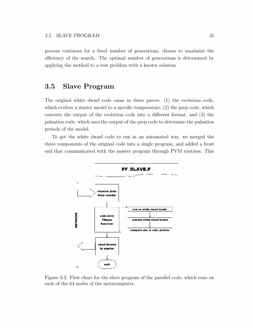
To get the white dwarf code to run in an automated way, we merged the
three components of the original code into a single program, and added a front
end that communicated with the master program through PVM routines. This
Figure 3.2: Flow chart for the slave program of the parallel code, which runs oneach of the 64 nodes of the metacomputer.
32 CHAPTER 3. PARALLEL GENETIC ALGORITHM
code (FF SLAVE.F) constitutes the slave program, and is run on each node of
the metacomputer. A full listing of this code is included in Appendix C, and a
flow chart is shown in Figure 3.2.
The operation of the slave program is relatively simple. Once it is started
by the master program, it receives a set of parameters from the network. It
then calls the fitness function (the white dwarf code) with these parameters as
arguments. The fitness function evolves a white dwarf model with characteristics
specified by the parameters, determines the pulsation periods of this model, and
then compares the calculated periods to the observed periods of a real white
dwarf. A fitness based on how well the two sets of periods match is returned
to the main program, which sends it to the master program over the network.
The node is then ready to run the slave program again and receive a new set of
parameters from the master program.
Chapter 4
Forward Modeling
“Why do we always find a lost screwdriver in the last place we look?”
—Joe Wampler
4.1 Introduction
Having developed the hardware and software for the genetic-algorithm-based
approach to model fitting, we were finally ready to learn something about white
dwarf stars. There are presently three known classes of pulsating white dwarfs.
The hottest class are the planetary nebula nucleus variables (PNNVs), which
have atmospheres of ionized helium and are also called DOVs. These objects
require detailed calculations that evolve a main sequence stellar model to the
pre-white dwarf phase to yield accurate pulsation periods. The two cooler classes
are the helium-atmosphere variable (DBV) and hydrogen-atmosphere variable
(DAV) white dwarfs. The pulsation periods of these objects can be calculated
accurately by evolving simpler, less detailed models called polytropes. The DAV
stars are generally modeled as a core of carbon and oxygen with an overlying
blanket of helium covered by a thin layer of hydrogen on the surface. The DBV
stars are the simplest of all, with no detectable hydrogen—only a helium layer
surrounding the carbon/oxygen core. In the spirit of solving the easier problem
first, we decided to apply the GA method to the DBV star GD 358.
33
34 CHAPTER 4. FORWARD MODELING
4.2 The DBV White Dwarf GD 358
During a survey of eighty-six suspected white dwarf stars in the Lowell GD lists,
Greenstein (1969) classified GD 358 as a helium atmosphere (DB) white dwarf
based on its spectrum. Photometric UBV and ubvy colors were later determined
by Bern & Wramdemark (1973) and Wegner (1979) respectively. Time-series
photometry by Winget, Robinson, Nather & Fontaine (1982) revealed the star to
be a pulsating variable—the first confirmation of a new class of variable (DBV)
white dwarfs predicted by Winget (1981).
In May 1990, GD 358 was the target of a coordinated observing run with
the Whole Earth Telescope (WET; Nather et al., 1990). The results of these
observations were reported by Winget et al. (1994), and the theoretical inter-
pretation was given in a companion paper by Bradley & Winget (1994b). They
found a series of nearly equally-spaced periods in the power spectrum which they
interpreted as non-radial g-mode pulsations of consecutive radial overtone. They
attempted to match the observed periods and the period spacing for these modes
using earlier versions of the same theoretical models we have used in this analysis
(see §4.3). Their optimization method involved computing a grid of models near
a first guess determined from general scaling arguments and analytical relations
developed by Kawaler (1990), Kawaler & Weiss (1990), Brassard et al. (1992),
and Bradley, Winget & Wood (1993).
4.3 DBV White Dwarf Models
4.3.1 Defining the Parameter-Space
The most important parameters affecting the pulsation properties of DBV white
dwarf models are the total stellar mass (M∗), the effective temperature (Teff),
and the mass of the atmospheric helium layer (MHe). We wanted to be careful
to avoid introducing any subjective bias into the best-fit determination simply
by defining the range of the search too narrowly. For this reason, we specified
the range for each parameter based only on the physics of the model, and on
observational constraints.
4.3. DBV WHITE DWARF MODELS 35
The distribution of masses for isolated white dwarf stars, generally inferred
from measurements of log g, is strongly peaked near 0.6 M¯ with a full width at
half maximum (FWHM) of about 0.1 M¯ (Napiwotzki, Green & Saffer, 1999).
Isolated main sequence stars with masses near the limit for helium ignition pro-
duce C/O cores more massive than about 0.45 M¯, so white dwarfs with masses
below this limit must have helium cores (Sweigart, Greggio & Renzini, 1990;
Napiwotzki, Green & Saffer, 1999). However, the universe is not presently old
enough to produce helium core white dwarfs through single star evolution. We
confine our search to masses between 0.45 M¯ and 0.95 M¯. Although some
white dwarfs are known to be more massive than the upper limit of our search,
these represent a very small fraction of the total population and, for reasonable
assumptions about the mass-radius relation, all known DBVs appear to have
masses within the range of our search (Beauchamp et al., 1999).
The span of temperatures within which DB white dwarfs are pulsationally
unstable is known as the DB instability strip. The precise location of this strip
is the subject of some debate, primarily because of difficulties in matching the
temperature scales from ultraviolet and optical spectroscopy and the possibility
of hiding trace amounts of hydrogen in the envelope (Beauchamp et al., 1999).
The most recent temperature determinations for the 8 known DBV stars were
done by Beauchamp et al. (1999). These measurements, depending on various
assumptions, place the red edge as low as 21,800 K, and the blue edge as high as
27,800 K. Our search includes all temperatures between 20,000 K and 30,000 K.
The mass of the atmospheric helium layer must not be greater than about
10−2 M∗ or the pressure of the overlying material would theoretically initiate
helium burning at the base of the envelope. At the other extreme, none of our
models pulsate for helium layer masses less than about 10−8 M∗ over the entire
temperature range we are considering (Bradley & Winget, 1994a). The practical
limit is actually slightly larger than this theoretical limit, and is a function of
mass. For the most massive white dwarfs we consider, our models run smoothly
with a helium layer as thin as 5× 10⁻⁸ M∗, while for the least massive the limit
is 4× 10⁻⁷ M∗ (see Figure 4.1).
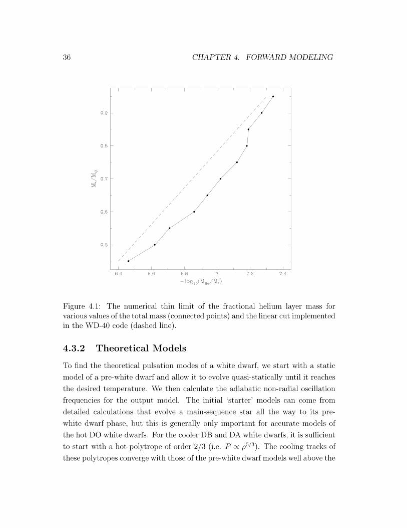
36 CHAPTER 4. FORWARD MODELING
Figure 4.1: The numerical thin limit of the fractional helium layer mass forvarious values of the total mass (connected points) and the linear cut implementedin the WD-40 code (dashed line).
4.3.2 Theoretical Models
To find the theoretical pulsation modes of a white dwarf, we start with a static
model of a pre-white dwarf and allow it to evolve quasi-statically until it reaches
the desired temperature. We then calculate the adiabatic non-radial oscillation
frequencies for the output model. The initial ‘starter’ models can come from
detailed calculations that evolve a main-sequence star all the way to its pre-
white dwarf phase, but this is generally only important for accurate models of
the hot DO white dwarfs. For the cooler DB and DA white dwarfs, it is sufficient
to start with a hot polytrope of order 2/3 (i.e. P ∝ ρ5/3). The cooling tracks of
these polytropes converge with those of the pre-white dwarf models well above the
4.3. DBV WHITE DWARF MODELS 37
temperatures at which DB and DA white dwarfs are observed to be pulsationally
unstable (Wood, 1990).
To allow fitting for the total mass, we generated a grid of 100 starter models
with masses between 0.45 and 0.95M¯. The entire grid originated from a 0.6M¯
carbon-core polytrope starter model. We performed a homology transform on
this model to generate three new masses: 0.65, 0.75, and 0.85 M¯. We relaxed
each of these three, and then used all four to generate the grid. All models
with masses below 0.6 M¯ were generated by a direct homology transform of
the original 0.6 M¯ polytrope. For masses between 0.605→ 0.745 M¯ and from
0.755 → 0.895 M¯, we used homology transforms of the relaxed 0.65 M¯ and
0.75 M¯ models respectively. The models with masses greater than 0.9 M¯ were
homology transforms of the relaxed 0.85 M¯ model.
To evolve a starter model to a specific temperature, we used the White Dwarf
Evolution Code (WDEC) described in detail by Lamb & Van Horn (1975) and
by Wood (1990). This code was originally written by Martin Schwarzschild,
and has subsequently been updated and modified by many others including:
Kutter & Savedoff (1969), Lamb & Van Horn (1975), Winget (1981), Kawaler
(1986), Wood (1990), Bradley (1993), and Montgomery (1998). The equation
of state (EOS) for the cores of our models come from Lamb (1974), and from
Fontaine, Graboske & Van Horn (1977) for the envelopes. We use the updated
OPAL opacity tables from Iglesias & Rogers (1993), neutrino rates from Itoh et
al. (1996), and the ML3 mixing-length prescription of Bohm & Cassinelli (1971).
The evolution calculations for the core are fully self-consistent, but the envelope is
treated separately. The core and envelope are stitched together and the envelope
is adjusted to match the boundary conditions at the interface. Adjusting the
helium layer mass involves stitching an envelope with the desired thickness onto
the core before starting the evolution. Because this is done while the model
is still very hot, there is plenty of time to reach equilibrium before the model
approaches the final temperature.
We determined the pulsation frequencies of the output models using the adia-
batic non-radial oscillation (ANRO) code described by Kawaler (1986), originally
written by Carl Hansen, which solves the pulsation equations using the Runge-
Kutta-Fehlberg method.
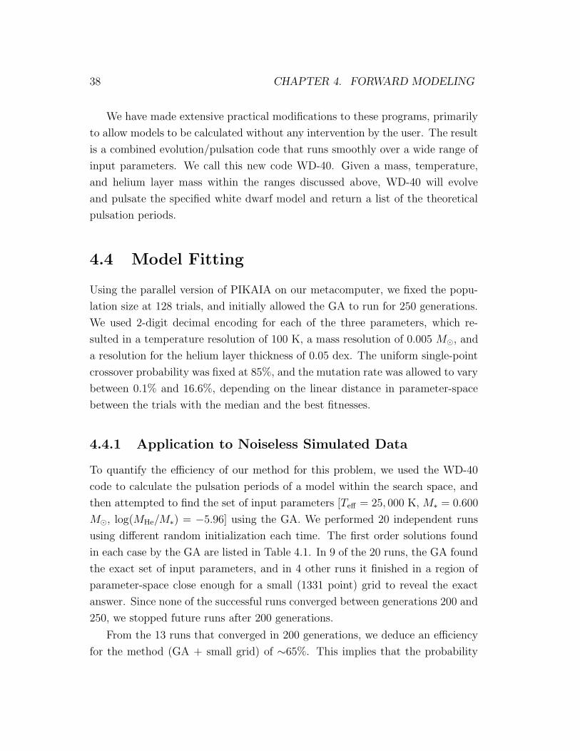
38 CHAPTER 4. FORWARD MODELING
We have made extensive practical modifications to these programs, primarily
to allow models to be calculated without any intervention by the user. The result
is a combined evolution/pulsation code that runs smoothly over a wide range of
input parameters. We call this new code WD-40. Given a mass, temperature,
and helium layer mass within the ranges discussed above, WD-40 will evolve
and pulsate the specified white dwarf model and return a list of the theoretical
pulsation periods.
4.4 Model Fitting
Using the parallel version of PIKAIA on our metacomputer, we fixed the popu-
lation size at 128 trials, and initially allowed the GA to run for 250 generations.
We used 2-digit decimal encoding for each of the three parameters, which re-
sulted in a temperature resolution of 100 K, a mass resolution of 0.005 M¯, and
a resolution for the helium layer thickness of 0.05 dex. The uniform single-point
crossover probability was fixed at 85%, and the mutation rate was allowed to vary
between 0.1% and 16.6%, depending on the linear distance in parameter-space
between the trials with the median and the best fitnesses.
4.4.1 Application to Noiseless Simulated Data
To quantify the efficiency of our method for this problem, we used the WD-40
code to calculate the pulsation periods of a model within the search space, and
then attempted to find the set of input parameters [Teff = 25, 000 K, M∗ = 0.600
M¯, log(MHe/M∗) = −5.96] using the GA. We performed 20 independent runs
using different random initialization each time. The first order solutions found
in each case by the GA are listed in Table 4.1. In 9 of the 20 runs, the GA found
the exact set of input parameters, and in 4 other runs it finished in a region of
parameter-space close enough for a small (1331 point) grid to reveal the exact
answer. Since none of the successful runs converged between generations 200 and
250, we stopped future runs after 200 generations.
From the 13 runs that converged in 200 generations, we deduce an efficiency
for the method (GA + small grid) of ∼65%. This implies that the probability
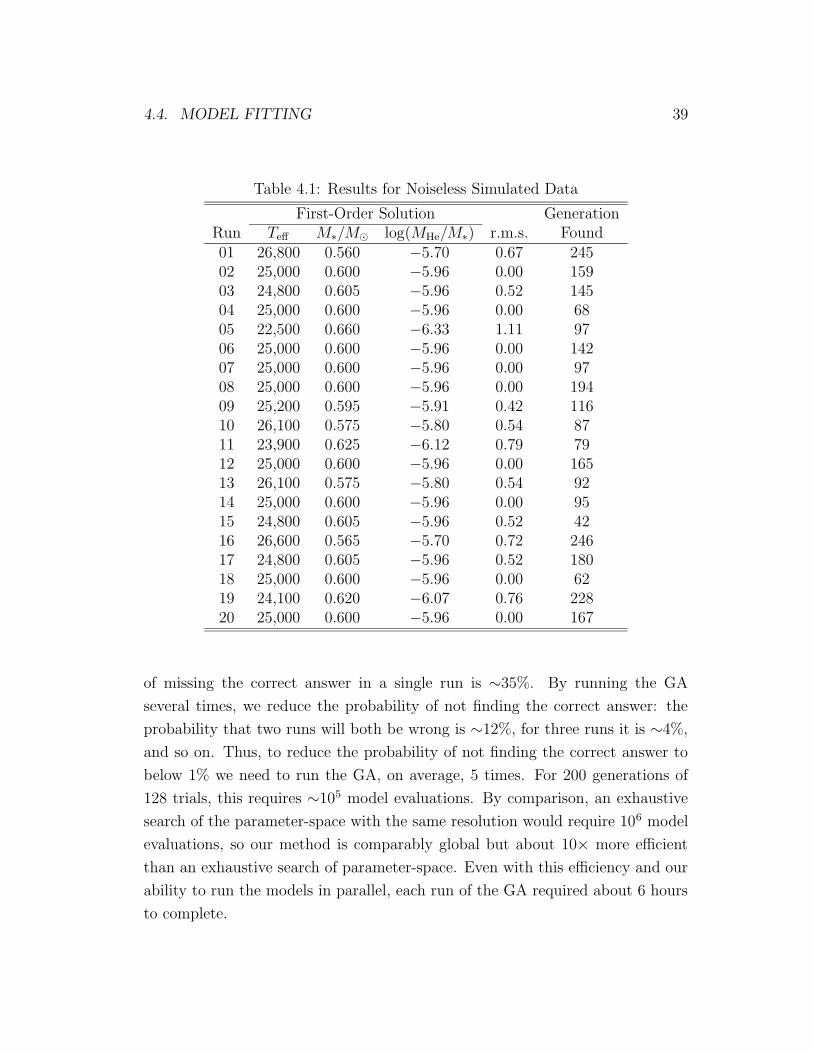
4.4. MODEL FITTING 39
Table 4.1: Results for Noiseless Simulated Data
First-Order Solution GenerationRun Teff M∗/M¯ log(MHe/M∗) r.m.s. Found01 26,800 0.560 −5.70 0.67 24502 25,000 0.600 −5.96 0.00 15903 24,800 0.605 −5.96 0.52 14504 25,000 0.600 −5.96 0.00 6805 22,500 0.660 −6.33 1.11 9706 25,000 0.600 −5.96 0.00 14207 25,000 0.600 −5.96 0.00 9708 25,000 0.600 −5.96 0.00 19409 25,200 0.595 −5.91 0.42 11610 26,100 0.575 −5.80 0.54 8711 23,900 0.625 −6.12 0.79 7912 25,000 0.600 −5.96 0.00 16513 26,100 0.575 −5.80 0.54 9214 25,000 0.600 −5.96 0.00 9515 24,800 0.605 −5.96 0.52 4216 26,600 0.565 −5.70 0.72 24617 24,800 0.605 −5.96 0.52 18018 25,000 0.600 −5.96 0.00 6219 24,100 0.620 −6.07 0.76 22820 25,000 0.600 −5.96 0.00 167
of missing the correct answer in a single run is ∼35%. By running the GA
several times, we reduce the probability of not finding the correct answer: the
probability that two runs will both be wrong is ∼12%, for three runs it is ∼4%,
and so on. Thus, to reduce the probability of not finding the correct answer to
below 1% we need to run the GA, on average, 5 times. For 200 generations of
128 trials, this requires ∼105 model evaluations. By comparison, an exhaustive
search of the parameter-space with the same resolution would require 106 model
evaluations, so our method is comparably global but about 10× more efficient
than an exhaustive search of parameter-space. Even with this efficiency and our
ability to run the models in parallel, each run of the GA required about 6 hours
to complete.
40 CHAPTER 4. FORWARD MODELING
4.4.2 The Effect of Gaussian Noise
Having established that the GA could find the correct answer for noiseless data,
we wanted to see how noise on the frequencies might affect it. Before adding noise
to the input frequencies, we attempted to characterize the actual noise present
on frequencies determined from a WET campaign. We approached this problem
in two different ways.
First, we tried to characterize the noise empirically by looking at the differ-
ences between the observed and predicted linear combination frequencies. When
we take the Fourier Transform of the long light curves from WET observations,
we are effectively decomposing the signal into perfect sinusoidal components of
various frequencies. The actual light variations arising from a single pulsation
mode are generally not perfect sinusoids, and the amplitude often varies on rela-
tively short timescales. This leads to significant power in the Fourier Transform
at integer multiples and fractions of the real pulsation frequency. These so-called
harmonics and sub-harmonics are examples of linear combination frequencies,
but they are not nearly as prevalent as the combinations that arise from the
interaction of different pulsation modes in the observed light curves.
When two pulsation modes with different frequencies f1 and f2 are present,
the resulting light curve shows oscillations at the sum of the two frequencies
f1 + f2. As the frequencies go into and out of phase or “beat” with each other,
the amplitude of the light variation grows and shrinks in a periodic manner at a
frequency equal to the difference of the two components f1−f2. If the amplitude
of the beating is smaller than expected due to some non-linear effect, then the
Fourier Transform will reveal power not only at the real pulsation frequencies, but
also at these combination frequencies. If we can properly identify the pulsation
modes that produce a specific linear combination, it allows us to estimate the
uncertainty on our frequency measurements because the combination should show
up at a precise sum or difference.
We used the mode identifications of Vuille et al. (2000) from the 1994 WET
run on GD 358. There were a total of 63 combinations identified: 20 sum and
11 difference frequencies of 2-mode combinations, 30 sum and difference 3-mode
combinations, and 2 combinations involving 4 modes. We used the measured fre-
quencies of the parent modes to predict the frequency of each linear combination,
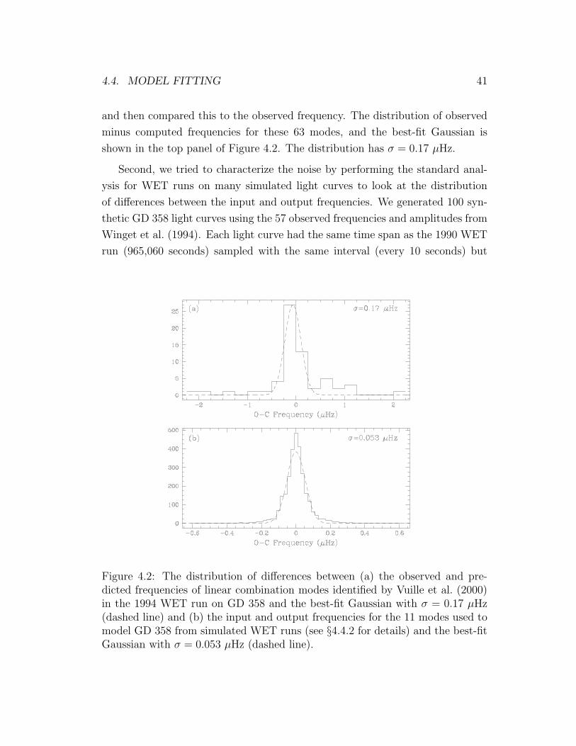
4.4. MODEL FITTING 41
and then compared this to the observed frequency. The distribution of observed
minus computed frequencies for these 63 modes, and the best-fit Gaussian is
shown in the top panel of Figure 4.2. The distribution has σ = 0.17 µHz.
Second, we tried to characterize the noise by performing the standard anal-
ysis for WET runs on many simulated light curves to look at the distribution
of differences between the input and output frequencies. We generated 100 syn-
thetic GD 358 light curves using the 57 observed frequencies and amplitudes from
Winget et al. (1994). Each light curve had the same time span as the 1990 WET
run (965,060 seconds) sampled with the same interval (every 10 seconds) but
Figure 4.2: The distribution of differences between (a) the observed and pre-dicted frequencies of linear combination modes identified by Vuille et al. (2000)in the 1994 WET run on GD 358 and the best-fit Gaussian with σ = 0.17 µHz(dashed line) and (b) the input and output frequencies for the 11 modes used tomodel GD 358 from simulated WET runs (see §4.4.2 for details) and the best-fitGaussian with σ = 0.053 µHz (dashed line).
42 CHAPTER 4. FORWARD MODELING
without any gaps in coverage. Although the noise in the observed light curves
was clearly time-correlated, we found that the distribution around the mean light
level for the comparison star after the standard reduction procedure was well rep-
resented by a Gaussian. So we added Gaussian noise to the simulated light curves
to yield a signal-to-noise ratio S/N ≈ 2, which is typical of the observed data.
We took the discrete Fourier Transform of each light curve, and identified peaks
in the same way as is done for real WET runs. We calculated the differences
between the input frequencies and those determined from the simulation for the
11 modes used in the seismological analysis by Bradley & Winget (1994b). The
distribution of these differences is shown in the bottom panel of Figure 4.2, along
with the best-fit Gaussian which has σ = 0.053 µHz. Because the noise measure-
ment from linear combination frequencies suffered from low-number statistics, we
adopted the noise estimate from the synthetic light curves for our studies of the
effect of noise on the GA method.
Using the same input model as in §4.4.1, we added random offsets drawn
from a Gaussian distribution with σ = 0.053 µHz to each of the frequencies. We
produced 10 sets of target frequencies from 10 unique realizations of the noise,
and then applied the GA method to each set. In all cases the best of 5 runs of the
GA found the exact set of parameters from the original input model, or a region
close enough to reveal the exact solution after calculating the small grid around
the first guess. To reassure ourselves that the success of the GA did not depend
strongly on the amount of noise added to the frequencies, we also performed fits
for several realizations of the larger noise estimate from the analysis of linear
combination frequencies. The method always succeeded in finding the original
input model.
4.4.3 Application to GD 358
Having thoroughly characterized the GA method, we finally applied it to real
data. We used the same 11 periods used by Bradley & Winget (1994b). As in
their analysis, we assumed that the periods were consecutive radial overtones and
that they were all ` = 1 modes (Winget et al., 1994, give detailed arguments to
support this assumption). Anticipating that the GA might have more difficulty
with non-synthetic data, we decided to perform a total of 10 GA runs for each
4.5. INITIAL RESULTS 43
core composition. This should reduce the chances of not finding the best answer
to less than about 3 in 10,000.
To facilitate comparison with previous results, we obtained fits for six different
combinations of core composition and internal chemical profiles: pure C, pure O,
and both “steep” and “shallow” internal chemical profiles for 50:50 and 20:80
C/O cores (see Bradley, Winget & Wood, 1993; Bradley & Winget, 1994b).
We also ran the GA with an alternate fitness criterion for the 50:50 C/O
“steep” case, which contains the best-fit model of Bradley & Winget (1994b).
Normally, the GA only attempts to match the pulsation periods. We repro-
grammed it to match both the periods and the period spacing, which was the
fitness criterion used by Bradley & Winget. Within the range of parameters they
considered, using this alternate fitness criterion, the GA found best-fit model
parameters consistent with Bradley & Winget’s solution.
4.5 Initial Results
The general features of the 3-dimensional parameter-space for GD 358 are illus-
trated in Figure 4.3. All combinations of parameters found by the GA for a 50:50
C/O steep core having r.m.s. period differences smaller than 3 seconds are shown
as square points in this plot. The two panels are orthogonal projections of the
search space, so each point in the left panel corresponds one-to-one with a point
in the right panel. Essentially, Figure 4.3 shows which combinations of model
parameters yield reasonably good matches to the periods observed in GD 358 for
this core composition.
The most obvious feature of the parameter-space is the presence of more
than one region that yields a good match to the observations. Generally, the
good fits seem to cluster in two families corresponding to thick and thin helium
layers. This is the first exciting result of applying the GA method. The best-fit
solution of Bradley & Winget (1994b) falls in the family with thin helium layers.
This solution was problematic at the time because the earlier asteroseismological
investigation of the hot white dwarf PG 1159-035 (Winget et al., 1991) implied
that it had a relatively thick helium layer. If there is an evolutionary connection
between PG 1159 stars and the DBVs, it was more difficult to understand if the
helium layers were significantly different. If a better solution for GD 358 exists
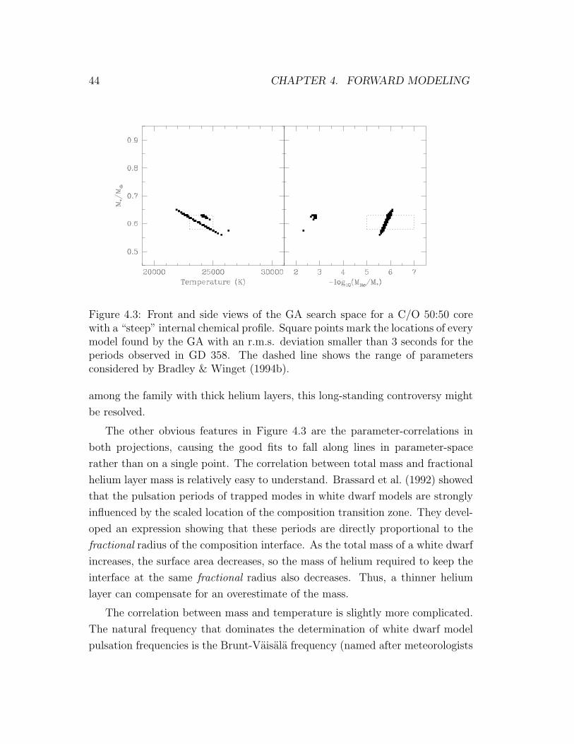
44 CHAPTER 4. FORWARD MODELING
Figure 4.3: Front and side views of the GA search space for a C/O 50:50 corewith a “steep” internal chemical profile. Square points mark the locations of everymodel found by the GA with an r.m.s. deviation smaller than 3 seconds for theperiods observed in GD 358. The dashed line shows the range of parametersconsidered by Bradley & Winget (1994b).
among the family with thick helium layers, this long-standing controversy might
be resolved.
The other obvious features in Figure 4.3 are the parameter-correlations in
both projections, causing the good fits to fall along lines in parameter-space
rather than on a single point. The correlation between total mass and fractional
helium layer mass is relatively easy to understand. Brassard et al. (1992) showed
that the pulsation periods of trapped modes in white dwarf models are strongly
influenced by the scaled location of the composition transition zone. They devel-
oped an expression showing that these periods are directly proportional to the
fractional radius of the composition interface. As the total mass of a white dwarf
increases, the surface area decreases, so the mass of helium required to keep the
interface at the same fractional radius also decreases. Thus, a thinner helium
layer can compensate for an overestimate of the mass.
The correlation between mass and temperature is slightly more complicated.
The natural frequency that dominates the determination of white dwarf model
pulsation frequencies is the Brunt-Vaisala frequency (named after meteorologists
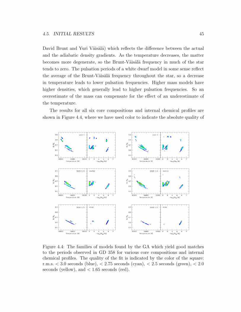
4.5. INITIAL RESULTS 45
David Brunt and Yuri Vaisala) which reflects the difference between the actual
and the adiabatic density gradients. As the temperature decreases, the matter
becomes more degenerate, so the Brunt-Vaisala frequency in much of the star
tends to zero. The pulsation periods of a white dwarf model in some sense reflect
the average of the Brunt-Vaisala frequency throughout the star, so a decrease
in temperature leads to lower pulsation frequencies. Higher mass models have
higher densities, which generally lead to higher pulsation frequencies. So an
overestimate of the mass can compensate for the effect of an underestimate of
the temperature.
The results for all six core compositions and internal chemical profiles are
shown in Figure 4.4, where we have used color to indicate the absolute quality of
Figure 4.4: The families of models found by the GA which yield good matchesto the periods observed in GD 358 for various core compositions and internalchemical profiles. The quality of the fit is indicated by the color of the square:r.m.s. < 3.0 seconds (blue), < 2.75 seconds (cyan), < 2.5 seconds (green), < 2.0seconds (yellow), and < 1.65 seconds (red).
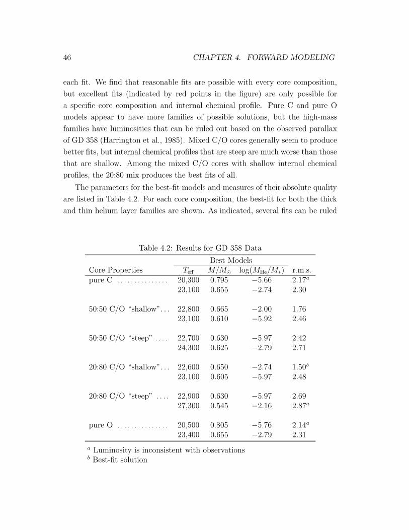
46 CHAPTER 4. FORWARD MODELING
each fit. We find that reasonable fits are possible with every core composition,
but excellent fits (indicated by red points in the figure) are only possible for
a specific core composition and internal chemical profile. Pure C and pure O
models appear to have more families of possible solutions, but the high-mass
families have luminosities that can be ruled out based on the observed parallax
of GD 358 (Harrington et al., 1985). Mixed C/O cores generally seem to produce
better fits, but internal chemical profiles that are steep are much worse than those
that are shallow. Among the mixed C/O cores with shallow internal chemical
profiles, the 20:80 mix produces the best fits of all.
The parameters for the best-fit models and measures of their absolute quality
are listed in Table 4.2. For each core composition, the best-fit for both the thick
and thin helium layer families are shown. As indicated, several fits can be ruled
Table 4.2: Results for GD 358 Data
Best ModelsCore Properties Teff M/M¯ log(MHe/M∗) r.m.s.pure C . . . . . . . . . . . . . . . 20,300 0.795 −5.66 2.17a
23,100 0.655 −2.74 2.30
50:50 C/O “shallow”. . . 22,800 0.665 −2.00 1.7623,100 0.610 −5.92 2.46
50:50 C/O “steep” . . . . 22,700 0.630 −5.97 2.4224,300 0.625 −2.79 2.71
20:80 C/O “shallow”. . . 22,600 0.650 −2.74 1.50b
23,100 0.605 −5.97 2.48
20:80 C/O “steep” . . . . 22,900 0.630 −5.97 2.6927,300 0.545 −2.16 2.87a
pure O . . . . . . . . . . . . . . . 20,500 0.805 −5.76 2.14a
23,400 0.655 −2.79 2.31
a Luminosity is inconsistent with observationsb Best-fit solution
4.6. INTERNAL COMPOSITION & STRUCTURE 47
out based on their luminosities. Our new best-fit model for GD 358 has a mass
and temperature marginally consistent with those inferred from spectroscopy.
4.6 Internal Composition & Structure
The initial 3-parameter fits to GD 358 make it clear that both the central oxygen
abundance and the shape of the internal chemical profile should be treated as
free parameters. We modified our code to allow any central oxygen mass fraction
(XO) between 0.00 and 1.00 with a resolution of 1 percent. To explore different
chemical profiles we fixed XO to its central value out to a fractional mass pa-
rameter (q) which varied between 0.10 and 0.85 with a resolution of 0.75 percent.
From this point, we forced XO to decrease linearly in mass to zero oxygen at the
95 percent mass point.
This parameterization is a generalized form of the “steep” and “shallow”
profiles. We used these profiles so that our results could be easily compared to
earlier work by Wood (1990) and Bradley, Winget & Wood (1993). The latter
authors define both profiles in their Figure 1. The “shallow” profile corresponds
approximately to q = 0.5, and “steep” corresponds roughly to q = 0.8. However,
in our generalized parameterization we have moved the point where the oxygen
abundance goes to zero from a fractional mass of 0.9 out to a fractional mass of
0.95. This coincides with the boundary in our models between the self-consistent
core and the envelope, where we describe the He/C transition using a diffusion
equilibrium profile from the method of Arcoragi & Fontaine (1980) with diffusion
exponents of ±3. We do not presently include oxygen in the envelopes, so the
mass fraction of oxygen must drop to zero by this point.
We calculated the magnitude of deviations from the mean period spacing for
models using our profiles compared to those due to smooth profiles from recent
theoretical calculations by Salaris et al. (1997). The smooth theoretical profiles
caused significantly larger deviations, so we conclude that the abrupt changes in
the oxygen abundance resulting from our parameterization do not have an un-
usually large effect on the period spacing. Although the actual chemical profiles
will almost certainly differ from the profiles resulting from our simple parameter-
ization, we should still be able to probe the gross features of the interior structure
48 CHAPTER 4. FORWARD MODELING
by matching one or another linear region of the presumably more complicated
physical profiles.
We used the same ranges and resolution for M∗, Teff , and MHe as in the initial
study, so the search space for this 5-parameter problem is 10,000 times larger
than for the 3-parameter case. Initially we tried to vary all 5 parameters simul-
taneously, but this proved to be impractical because of the parameter-correlation
between M∗ and q. The pulsation properties of the models depend on the radial
location in the chemical profile where the oxygen mass fraction begins to change.
If the GA finds a combination of M∗ and q that yields a reasonably good fit
to the data, most changes to either one of them by itself will not improve the
fit. As a consequence, simultaneous changes to both parameters are required to
find a better fit, and since this is not very probable the GA must run for a very
long time. Tests on synthetic data for the full 5-parameter problem yielded only
a 10 percent probability of finding the input model even when we ran for 2000
generations—ten times longer than for the 3-parameter case. By contrast, when
we used a fixed value of q and repeated the test with only 4 free parameters, the
GA found the input model in only 400 generations for 8 out of 10 runs. Even
better, by fixing the mass and allowing q to vary, it took only 250 generations
to find the input model in 7 out of 10 runs. This suggests that it might be more
efficient to alternate between these two subsets of 4 parameters, fixing the fifth
parameter each time to its best-fit value from the previous iteration, until the
results of both fits are identical.
Since we do not know a priori the precise mass of the white dwarf, we need
to ensure that this iterative 4-parameter approach will work even when the mass
is initially fixed at an incorrect value. To test this, we calculated the pulsation
periods of the best-fit 0.65 M¯ model for GD 358 from Table 4.2 and then itera-
tively applied the two 4-parameter fitting routines, starting with the mass fixed
at 0.60 M¯—an offset comparable to the discrepancy between the mass found in
Table 4.2 and the value found by Bradley & Winget (1994b). The series of fits
leading to the input model are shown in Table 4.3. This method required only
3 iterations, and for each iteration we performed 10 runs with different random
initialization to yield a probability of finding the best-fit much greater than 99.9
percent. In the end, the method required a total of 2.5× 10⁶ model evaluations
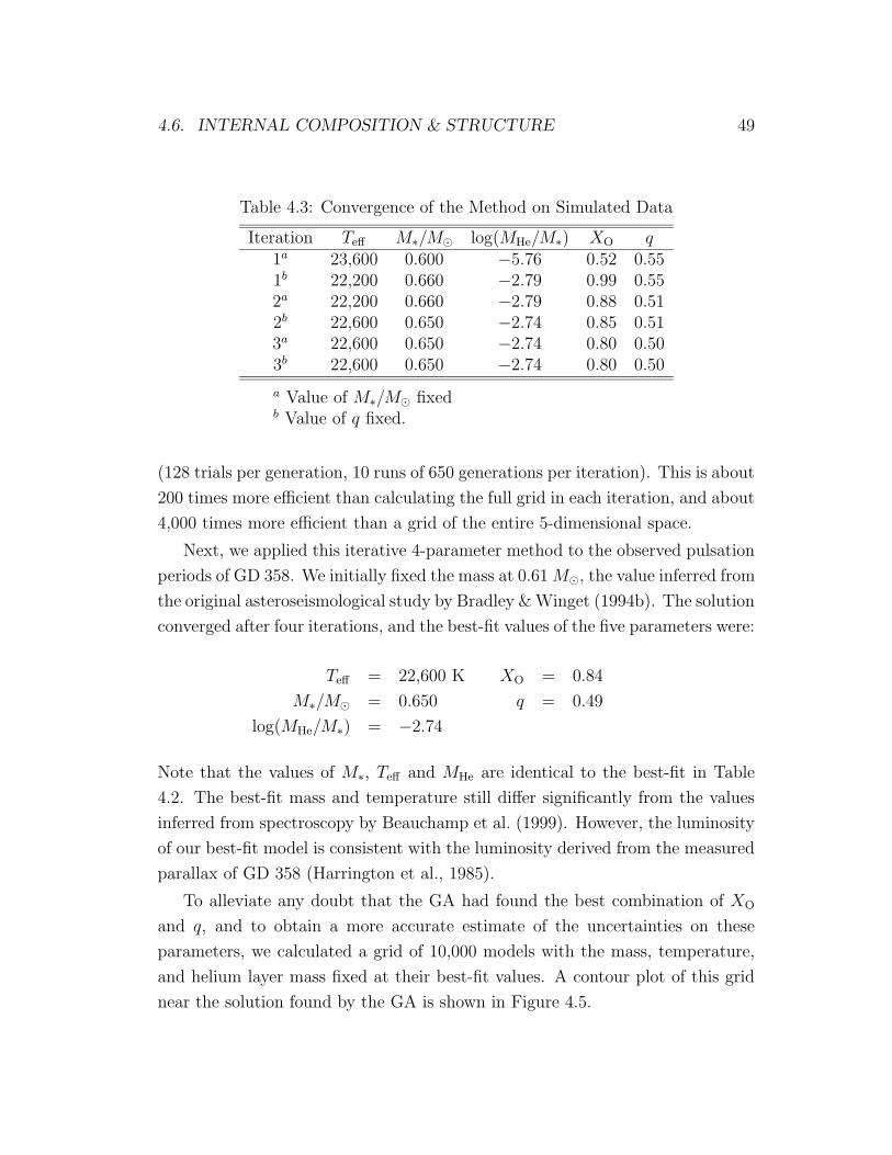
4.6. INTERNAL COMPOSITION & STRUCTURE 49
Table 4.3: Convergence of the Method on Simulated Data
Iteration Teff M∗/M¯ log(MHe/M∗) XO q1a 23,600 0.600 −5.76 0.52 0.551b 22,200 0.660 −2.79 0.99 0.552a 22,200 0.660 −2.79 0.88 0.512b 22,600 0.650 −2.74 0.85 0.513a 22,600 0.650 −2.74 0.80 0.503b 22,600 0.650 −2.74 0.80 0.50
a Value of M∗/M¯ fixedb Value of q fixed.
(128 trials per generation, 10 runs of 650 generations per iteration). This is about
200 times more efficient than calculating the full grid in each iteration, and about
4,000 times more efficient than a grid of the entire 5-dimensional space.
Next, we applied this iterative 4-parameter method to the observed pulsation
periods of GD 358. We initially fixed the mass at 0.61M¯, the value inferred from
the original asteroseismological study by Bradley &Winget (1994b). The solution
converged after four iterations, and the best-fit values of the five parameters were:
Teff = 22,600 K XO = 0.84
M∗/M¯ = 0.650 q = 0.49
log(MHe/M∗) = −2.74
Note that the values of M∗, Teff and MHe are identical to the best-fit in Table
4.2. The best-fit mass and temperature still differ significantly from the values
inferred from spectroscopy by Beauchamp et al. (1999). However, the luminosity
of our best-fit model is consistent with the luminosity derived from the measured
parallax of GD 358 (Harrington et al., 1985).
To alleviate any doubt that the GA had found the best combination of XO
and q, and to obtain a more accurate estimate of the uncertainties on these
parameters, we calculated a grid of 10,000 models with the mass, temperature,
and helium layer mass fixed at their best-fit values. A contour plot of this grid
near the solution found by the GA is shown in Figure 4.5.
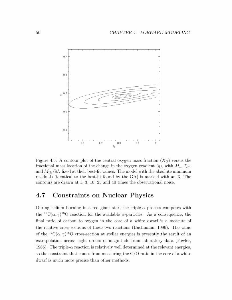
50 CHAPTER 4. FORWARD MODELING
Figure 4.5: A contour plot of the central oxygen mass fraction (XO) versus thefractional mass location of the change in the oxygen gradient (q), with M∗, Teff ,andMHe/M∗ fixed at their best-fit values. The model with the absolute minimumresiduals (identical to the best-fit found by the GA) is marked with an X. Thecontours are drawn at 1, 3, 10, 25 and 40 times the observational noise.
4.7 Constraints on Nuclear Physics
During helium burning in a red giant star, the triple-α process competes with
the 12C(α, γ)16O reaction for the available α-particles. As a consequence, the
final ratio of carbon to oxygen in the core of a white dwarf is a measure of
the relative cross-sections of these two reactions (Buchmann, 1996). The value
of the 12C(α, γ)16O cross-section at stellar energies is presently the result of an
extrapolation across eight orders of magnitude from laboratory data (Fowler,
1986). The triple-α reaction is relatively well determined at the relevant energies,
so the constraint that comes from measuring the C/O ratio in the core of a white
dwarf is much more precise than other methods.
4.7. CONSTRAINTS ON NUCLEAR PHYSICS 51
Adopting the central oxygen mass fraction from the 5-parameter best-fit for-
ward modeling (XO = 84 ± 3 percent) we can place preliminary constraints on
the 12C(α, γ)16O cross-section. Salaris et al. (1997) made detailed evolution-
ary calculations for main-sequence stellar models with masses between 1 and 7
M¯ to provide internal chemical profiles for the resulting white dwarfs. For the
bulk of the calculations they adopted the rate of Caughlan et al. (1985) for the12C(α, γ)16O reaction (S300 = 240 keV barns), but they also computed an evo-
lutionary sequence using the lower cross-section inferred by Woosley, Timmes &
Weaver (1993) from solar abundances (S300 = 170 keV barns). The chemical
profiles from both rates had the same general shape, but the oxygen abundances
were uniformly smaller for the lower rate. In both cases the C/O ratio was con-
stant out to the 50 percent mass point, a region easily probed by white dwarf
pulsations.
The central oxygen mass fraction is lower in higher mass white dwarf models.
The rate of the triple-α reaction (a three-body process) increases faster at higher
densities than does the 12C(α, γ)16O reaction. As a consequence, more helium is
used up in the production of carbon, and relatively less is available to produce
oxygen in higher mass models. Interpolating between the models of Salaris et
al. (1997) which used the higher value of the cross-section, we expect a central
oxygen mass fraction for a M∗ = 0.65 M¯ model of XhighO = 0.75. Using ad-
ditional calculations for the low rate (M. Salaris 2001, private communication),
the expected value is X lowO = 0.62. Extrapolating to the value inferred from our
5-parameter forward modeling, we estimate that the astrophysical S-factor at 300
keV for the 12C(α, γ)16O cross-section is in the range S300 = 290± 15 keV barns
(internal uncertainty only).

52 CHAPTER 4. FORWARD MODELING
Chapter 5
Reverse Approach
“The only real voyage of discovery consists not in seeking new land-
scapes but in having new eyes.”
—Marcel Proust
5.1 Introduction
The results of forward modeling with one adjustable point in the chemical profile
make it clear that information about the internal structure is contained in the
data, and we just need to learn how to extract it. If we want to test more compli-
cated adjustable profiles, forward modeling quickly becomes too computationally
expensive as the dimensionality of the search space increases. We need to devise
a more efficient approach to explore the myriad possibilities.
The natural frequency that dominates the determination of pulsation periods
in white dwarf models is the Brunt-Vaisala (BV) frequency, which we calculate
using the Modified Ledoux treatment described in Tassoul, Fontaine & Winget
(1990). To get a sense of how the pulsation periods depend on the BV frequency
in various regions of the model interior, we added a smooth perturbation to
the best-fit model of GD 358 from Table 4.2, moving it one shell at a time
from the center to the surface. The perturbation artificially decreased the BV
frequency across seven shells, with a maximum amplitude of 10 percent. We
monitored the effect on each of the pulsation periods as the perturbation moved
53
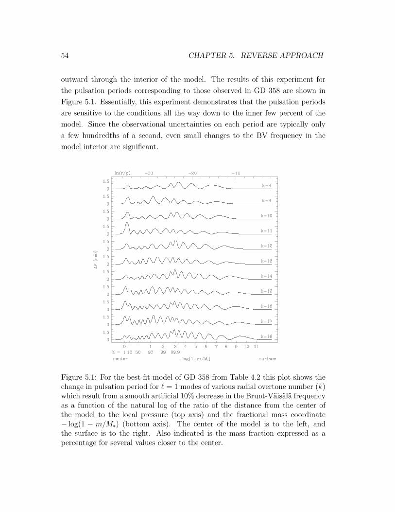
54 CHAPTER 5. REVERSE APPROACH
outward through the interior of the model. The results of this experiment for
the pulsation periods corresponding to those observed in GD 358 are shown in
Figure 5.1. Essentially, this experiment demonstrates that the pulsation periods
are sensitive to the conditions all the way down to the inner few percent of the
model. Since the observational uncertainties on each period are typically only
a few hundredths of a second, even small changes to the BV frequency in the
model interior are significant.
Figure 5.1: For the best-fit model of GD 358 from Table 4.2 this plot shows thechange in pulsation period for ` = 1 modes of various radial overtone number (k)which result from a smooth artificial 10% decrease in the Brunt-Vaisala frequencyas a function of the natural log of the ratio of the distance from the center ofthe model to the local pressure (top axis) and the fractional mass coordinate− log(1 − m/M∗) (bottom axis). The center of the model is to the left, andthe surface is to the right. Also indicated is the mass fraction expressed as apercentage for several values closer to the center.
5.2. MODEL PERTURBATIONS 55
5.2 Model Perturbations
The root-mean-square (r.m.s.) residuals between the observed pulsation periods
in GD 358 and those calculated for the best-fit from forward modeling are still
much larger than the observational noise. This suggests that either we have
left something important out of our model, or we have neglected to optimize
one or more of the parameters that could in principle yield a closer match to
the observations. To investigate the latter possibility, we introduced ad hoc
perturbations to the BV frequency of the best-fit model to see if the match
could be improved. Initially, we concentrated on the region of the Brunt-Vaisala
curve that corresponds to the internal chemical profile.
If we look at the BV frequency for models with the same mass, temperature,
helium layer mass, and central oxygen mass fraction but different internal chem-
ical profiles (see Figure 5.2) it becomes clear that the differences are localized.
In general, we find that changes in the composition gradient cause shifts in the
BV frequency. Moving across an interface where the gradient becomes steeper,
the BV frequency shifts higher; at an interface where the gradient becomes more
shallow, the BV frequency shifts lower. The greater the change in the gradient,
the larger the shift in the BV frequency.
5.2.1 Proof of Concept
We began by generating a model with the same mass, temperature, helium layer
mass, and internal composition as the best-fit from Table 4.2, but using a uniform
internal chemical profile with constant 20:80 C/O out to the 95 percent mass
point. We identified a sequence of 100 shells in this model spanning a range
of fractional mass from 0.20 to 0.97 and perturbed the BV frequency to try to
produce a better match to the observations. We parameterized the perturbation
as a linearly varying multiplicative factor applied to the BV frequency over a
range of shells, described by four parameters: (1) the innermost shell to perturb,
(2) the magnitude of the perturbation at the innermost shell, (3) the number of
shells in the perturbation range, and (4) the magnitude of the perturbation at
the outermost shell. These 4 parameters are sufficient to describe a profile with
two abrupt changes in the composition gradient.
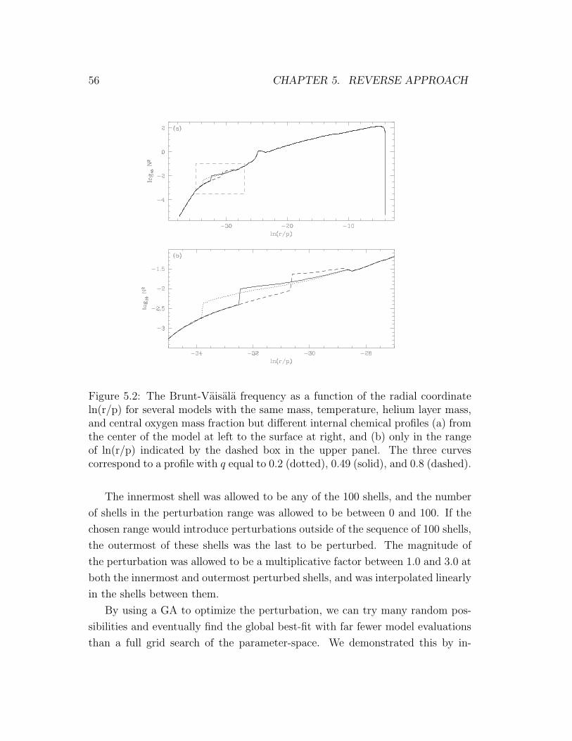
56 CHAPTER 5. REVERSE APPROACH
Figure 5.2: The Brunt-Vaisala frequency as a function of the radial coordinateln(r/p) for several models with the same mass, temperature, helium layer mass,and central oxygen mass fraction but different internal chemical profiles (a) fromthe center of the model at left to the surface at right, and (b) only in the rangeof ln(r/p) indicated by the dashed box in the upper panel. The three curvescorrespond to a profile with q equal to 0.2 (dotted), 0.49 (solid), and 0.8 (dashed).
The innermost shell was allowed to be any of the 100 shells, and the number
of shells in the perturbation range was allowed to be between 0 and 100. If the
chosen range would introduce perturbations outside of the sequence of 100 shells,
the outermost of these shells was the last to be perturbed. The magnitude of
the perturbation was allowed to be a multiplicative factor between 1.0 and 3.0 at
both the innermost and outermost perturbed shells, and was interpolated linearly
in the shells between them.
By using a GA to optimize the perturbation, we can try many random pos-
sibilities and eventually find the global best-fit with far fewer model evaluations
than a full grid search of the parameter-space. We demonstrated this by in-
5.2. MODEL PERTURBATIONS 57
troducing a particular perturbation to the model and determining the pulsation
periods. Using the same unperturbed model, we then attempted to find the pa-
rameters of the perturbation by matching the periods using the GA. In 9 out of
10 runs (500 generations of 64 trials), the GA found a first-order solution within
two grid points of the input perturbation. Thus, the GA combined with a small
(625 point) grid search yields a 90 percent probability of success for an individual
run. By repeating the process several times, the probability of finding the correct
answer quickly exceeds 99.9 percent, even while the number of model evaluations
required remains hundreds of times lower than a full grid of the parameter-space.
5.2.2 Application to GD 358
Having demonstrated that the method works on calculated model periods, we
applied it to the observed pulsation periods of GD 358. We began with a
model similar to the 5-parameter best-fit determined from forward modeling,
but again using a uniform internal chemical profile (constant 16:84 C/O out to
0.95 m/M∗). After the GA had found the best-fit perturbation for GD 358, we
reverse-engineered the corresponding chemical profile.
To accomplish this, we first looked in the unperturbed model for the fractional
mass corresponding to the innermost and outermost shells in the perturbation
range. We fixed the oxygen abundance to that of the unperturbed model from the
center out to the fractional mass of the innermost perturbed shell. The size of the
shift in the BV frequency is determined by how much the composition gradient
changes at this point, so we adjusted the oxygen abundance at the fractional
mass of the outermost perturbed shell until the change in the gradient produced
the required shift. Finally, we fixed the oxygen abundance to that value from
the outermost perturbed shell out to a fractional mass of 0.95, where it abruptly
goes to zero.
After we found the C/O profile of the best-fit perturbation in this way, we
fixed this reverse-engineered profile in the models and performed a new fit from
forward modeling with the GA to re-optimize the mass, temperature, helium layer
mass, and central oxygen mass fraction. The BV curve of the final model differs
slightly, of course, from that of the original uniform composition model with the
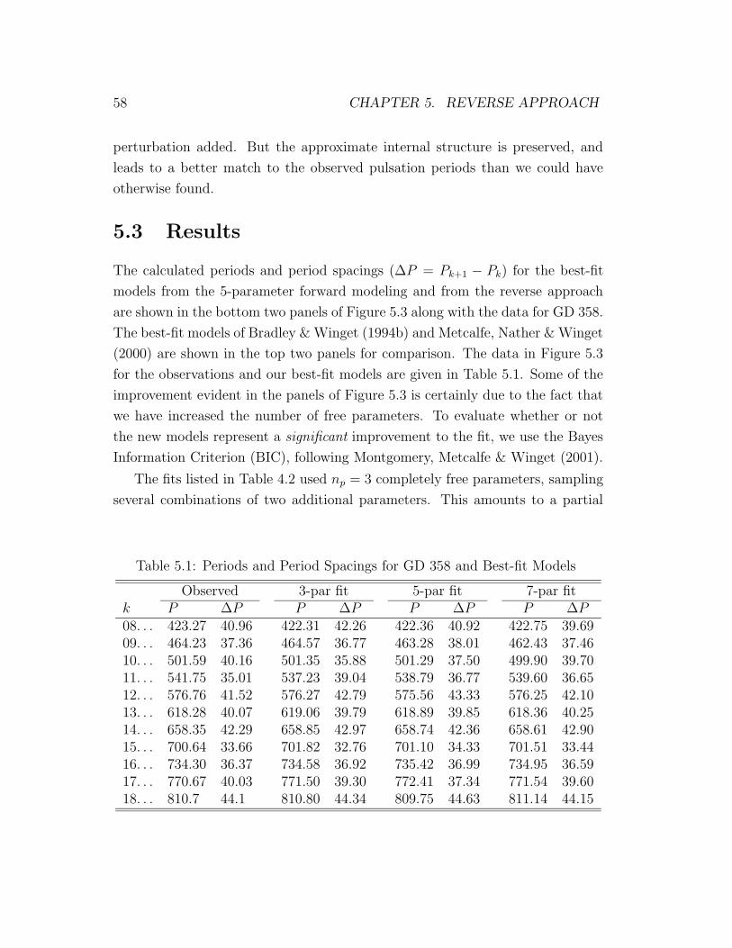
58 CHAPTER 5. REVERSE APPROACH
perturbation added. But the approximate internal structure is preserved, and
leads to a better match to the observed pulsation periods than we could have
otherwise found.
5.3 Results
The calculated periods and period spacings (∆P = Pk+1 − Pk) for the best-fit
models from the 5-parameter forward modeling and from the reverse approach
are shown in the bottom two panels of Figure 5.3 along with the data for GD 358.
The best-fit models of Bradley & Winget (1994b) and Metcalfe, Nather & Winget
(2000) are shown in the top two panels for comparison. The data in Figure 5.3
for the observations and our best-fit models are given in Table 5.1. Some of the
improvement evident in the panels of Figure 5.3 is certainly due to the fact that
we have increased the number of free parameters. To evaluate whether or not
the new models represent a significant improvement to the fit, we use the Bayes
Information Criterion (BIC), following Montgomery, Metcalfe & Winget (2001).
The fits listed in Table 4.2 used np = 3 completely free parameters, sampling
several combinations of two additional parameters. This amounts to a partial
Table 5.1: Periods and Period Spacings for GD 358 and Best-fit Models
Observed 3-par fit 5-par fit 7-par fitk P ∆P P ∆P P ∆P P ∆P08. . . 423.27 40.96 422.31 42.26 422.36 40.92 422.75 39.6909. . . 464.23 37.36 464.57 36.77 463.28 38.01 462.43 37.4610. . . 501.59 40.16 501.35 35.88 501.29 37.50 499.90 39.7011. . . 541.75 35.01 537.23 39.04 538.79 36.77 539.60 36.6512. . . 576.76 41.52 576.27 42.79 575.56 43.33 576.25 42.1013. . . 618.28 40.07 619.06 39.79 618.89 39.85 618.36 40.2514. . . 658.35 42.29 658.85 42.97 658.74 42.36 658.61 42.9015. . . 700.64 33.66 701.82 32.76 701.10 34.33 701.51 33.4416. . . 734.30 36.37 734.58 36.92 735.42 36.99 734.95 36.5917. . . 770.67 40.03 771.50 39.30 772.41 37.34 771.54 39.6018. . . 810.7 44.1 810.80 44.34 809.75 44.63 811.14 44.15
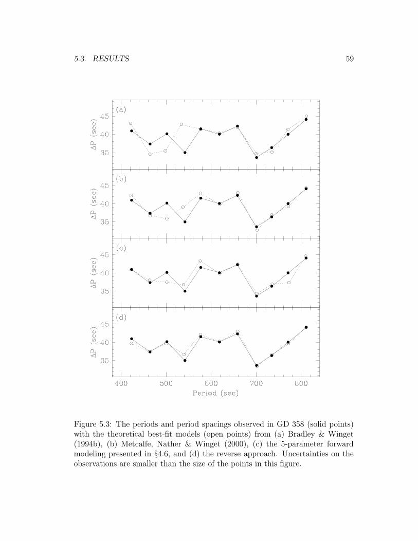
5.3. RESULTS 59
Figure 5.3: The periods and period spacings observed in GD 358 (solid points)with the theoretical best-fit models (open points) from (a) Bradley & Winget(1994b), (b) Metcalfe, Nather & Winget (2000), (c) the 5-parameter forwardmodeling presented in §4.6, and (d) the reverse approach. Uncertainties on theobservations are smaller than the size of the points in this figure.
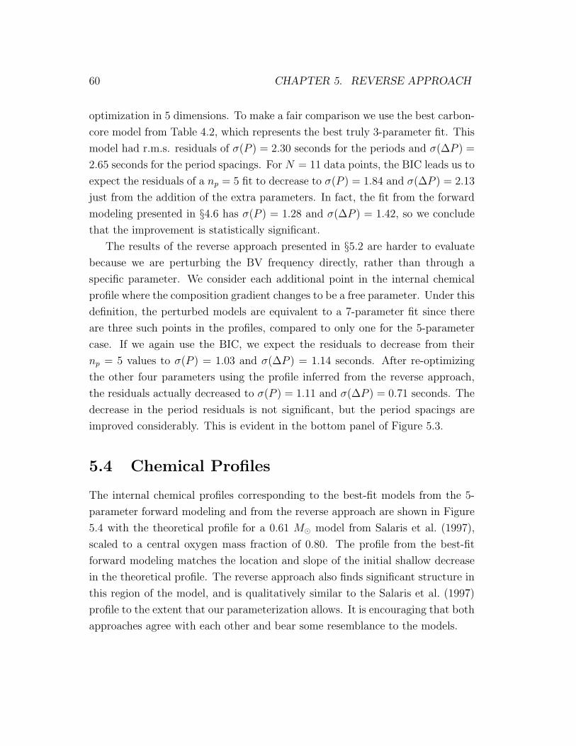
60 CHAPTER 5. REVERSE APPROACH
optimization in 5 dimensions. To make a fair comparison we use the best carbon-
core model from Table 4.2, which represents the best truly 3-parameter fit. This
model had r.m.s. residuals of σ(P ) = 2.30 seconds for the periods and σ(∆P ) =
2.65 seconds for the period spacings. For N = 11 data points, the BIC leads us to
expect the residuals of a np = 5 fit to decrease to σ(P ) = 1.84 and σ(∆P ) = 2.13
just from the addition of the extra parameters. In fact, the fit from the forward
modeling presented in §4.6 has σ(P ) = 1.28 and σ(∆P ) = 1.42, so we conclude
that the improvement is statistically significant.
The results of the reverse approach presented in §5.2 are harder to evaluate
because we are perturbing the BV frequency directly, rather than through a
specific parameter. We consider each additional point in the internal chemical
profile where the composition gradient changes to be a free parameter. Under this
definition, the perturbed models are equivalent to a 7-parameter fit since there
are three such points in the profiles, compared to only one for the 5-parameter
case. If we again use the BIC, we expect the residuals to decrease from their
np = 5 values to σ(P ) = 1.03 and σ(∆P ) = 1.14 seconds. After re-optimizing
the other four parameters using the profile inferred from the reverse approach,
the residuals actually decreased to σ(P ) = 1.11 and σ(∆P ) = 0.71 seconds. The
decrease in the period residuals is not significant, but the period spacings are
improved considerably. This is evident in the bottom panel of Figure 5.3.
5.4 Chemical Profiles
The internal chemical profiles corresponding to the best-fit models from the 5-
parameter forward modeling and from the reverse approach are shown in Figure
5.4 with the theoretical profile for a 0.61 M¯ model from Salaris et al. (1997),
scaled to a central oxygen mass fraction of 0.80. The profile from the best-fit
forward modeling matches the location and slope of the initial shallow decrease
in the theoretical profile. The reverse approach also finds significant structure in
this region of the model, and is qualitatively similar to the Salaris et al. (1997)
profile to the extent that our parameterization allows. It is encouraging that both
approaches agree with each other and bear some resemblance to the models.
5.4. CHEMICAL PROFILES 61
Figure 5.4: The internal oxygen profiles (top) and the corresponding region of theBrunt-Vaisala curves (bottom) for the best-fit forward model from §4.6 (dotted),the result of the best-fit reverse approach from §5.2 (dashed), and the scaledtheoretical calculations of Salaris et al. (1997) for comparison (solid).

62 CHAPTER 5. REVERSE APPROACH
Chapter 6
Conclusions
“The reasonable man adapts himself to the world; the unreasonable
one persists in trying to adapt the world to himself. Therefore all
progress depends on the unreasonable man.”
—George Bernard Shaw
6.1 Discussion of Results
The application of genetic-algorithm-based optimization to white dwarf pulsa-
tion models has turned out to be very fruitful. We are now confident that we can
rely on this approach to perform global searches and to provide not only objec-
tive, global best-fit models for the observed pulsation frequencies of DBV white
dwarfs, but also fairly detailed maps of the parameter-space as a natural byprod-
uct. This approach can easily be extended to treat the DAV stars and, with a
grid of more detailed starter models, eventually the DOVs. Ongoing all-sky sur-
veys promise to yield many new pulsating white dwarfs of all classes which will
require follow-up with the Whole Earth Telescope to obtain seismological data.
With the observation and analysis procedures in place, we will quickly be able
to understand the statistical properties of these ubiquitous and relatively simple
stellar objects. Our initial 3-parameter application of the method provided new
evidence that the pulsation frequencies of white dwarfs really are global oscilla-
tions. We refined our knowledge of the sensitivity of the models to the structure
63
64 CHAPTER 6. CONCLUSIONS
of the envelope, and we demonstrated that they are sensitive to the conditions
deep in the interior of the star, as suggested by previous work on crystallization
by Montgomery & Winget (1999).
The extension of the genetic-algorithm-based approach to optimize the in-
ternal composition and structure of our models of GD 358 yielded more ex-
citing results. The values of the 3 parameters considered in the initial study
(M∗, Teff ,MHe) were unchanged in the full 5-parameter fit, so we feel confident
that they are the most important for matching the gross period structure. The
efficiency of the GA relative to a grid search was much higher for this larger
parameter-space, and the ability of the method to find the global best-fit was
undiminished. The significant improvement to the fit made possible by includ-
ing XO and q as free parameters confirms that the observed pulsations really do
contain information about the hidden interiors of these stars.
Our best-fit solution has a thick helium layer, which should help to resolve the
controversy surrounding the evolutionary connection between the PG 1159 stars
and the DBVs. The helium layer mass for PG 1159-035 from the asteroseismolog-
ical investigation of Winget et al. (1991) was relatively thick, at ∼ 3× 10⁻³ M¯.
Kleinman et al. (1998) found good agreement with the observed pulsations in
the DAV star G29–38 using a similar helium layer mass. If the standard pic-
ture of white dwarf evolution is correct, with a slow cooling process connecting
all three classes of pulsators, then we would expect a similar structure for the
DBVs. The original best-fit model for GD 358 by Bradley & Winget (1994b)
had a relatively thin helium layer, at ∼ 1.2×10⁻⁶ M¯. This posed a problem for
the standard picture. Dehner & Kawaler (1995) treated this problem by includ-
ing time-dependent diffusive processes in their calculations, but admitted that it
still could not explain the presence of the DB gap, which is still an unresolved
problem. Our thick envelope solution also fits more comfortably within the evo-
lutionary scenario of a hot DB star becoming a carbon (DQ) white dwarf without
developing an anomalously high photospheric carbon abundance (Provencal et
al., 2000).
We have finally measured the central oxygen abundance in GD 358 and used
it to provide a preliminary constraint on the 12C(α, γ)16O nuclear reaction cross-
section. This reaction is one of the most important for understanding the late
6.1. DISCUSSION OF RESULTS 65
stages of stellar evolution and supernovae. Our preliminary value for the astro-
physical S-factor at 300 keV (S300 = 290± 15 keV barns) is high relative to most
published values. However, recent work on type Ia supernovae also favors a high
value to produce model light curves with a sufficiently slow rise to maximum
light (Hoeflich, Wheeler, & Thielemann, 1998). Fortunately, there are other ob-
servational consequences of the higher rate in the spectra of type Ia supernovae
models, so independent evidence should soon be possible.
More precise constraints on 12C(α, γ)16O from asteroseismology will require
additional detailed simulations like those of Salaris et al. (1997). By determining
the range of values for the cross-section that produce a central oxygen abundance
within the measurement uncertainties of XO, we should be able to surpass the
precision of the extrapolation from laboratory measurements by nearly an order
of magnitude. The quoted uncertainty on our preliminary measurement of the12C(α, γ)16O cross-section does not include systematic effects. There will cer-
tainly be some error associated with using our white dwarf models; we already
know that they aren’t perfect. There will also be some contribution to the un-
certainty from the assumptions built in to the chemical profiles of Salaris et al.
(1997), particularly from the description of convection.
We have demonstrated that the pulsation periods in our white dwarf models
are sensitive to the shape of the internal chemical profiles. We can use this shape
as a powerful diagnostic of other physical processes relevant to white dwarf model
interiors, such as convective overshooting and crystallization.
While they are still embedded in the cores of red giant models, the internal
chemical profiles of white dwarf models show a relatively constant C/O ratio near
the center, with a size determined by the extent of the helium-burning convective
region. The degree of mixing at the edge of this region is unknown, so a convective
overshooting parameter is used to investigate the effect of different assumptions
about mixing. With no convective overshooting, the final C/O ratio is constant
out to the 50% mass point; with the convective overshooting parameter fixed
at an empirically derived value, the central oxygen mass fraction is unchanged
a the level of a few percent, but the region with a constant C/O ratio extends
out to the 65% mass point. Further out in both cases the oxygen mass fraction
decreases as a result of the helium-burning shell moving toward the surface of
66 CHAPTER 6. CONCLUSIONS
the red giant model while gravitational contraction causes the temperature and
density to rise. This increases the efficiency of the triple-α reaction, producing
more carbon relative to oxygen.
Our parameterization of the internal chemical profile is not yet detailed enough
to probe all of the physical information contained in the actual profiles. Our re-
sults suggest that convective overshooting is not required to explain the internal
chemical profile of GD 358, to the extent that we can measure it at this time.
Additional fitting with more detailed evolutionary profiles will provide a definite
statement about convective overshooting, and will also provide constraints on
the 12C(α, γ)16O reaction over the range of temperatures and densities sampled
during the helium shell-burning phase.
Measurements of the internal chemical profiles will also provide a test of
phase separation and crystallization in more massive or cooler pulsating white
dwarf stars. The distribution of oxygen in the interior of a crystallizing white
dwarf model is significantly different from the chemical profile during the liquid
phase. The central oxygen mass fraction is higher, and the structure in the profile
virtually disappears (Salaris et al., 1997).
Our constraints presently come from measurements of a single white dwarf
star. Application of the GA fitting method to additional pulsating white dwarfs
will provide independent determinations of the central C/O ratio and internal
chemical profiles. These measurements should lead to the same nuclear physics,
or something is seriously wrong. Either way, we will learn something useful. It
would be best to apply this technique to another DBV star before applying it
to another class of pulsators, since it is still not certain that all of them are
produced in the same way. If we were to find a significantly different C/O ratio
for another kind of pulsator, it could be telling us something about differences in
the formation mechanisms.
The reverse approach to model-fitting has opened the door to exploring more
complicated chemical profiles, and the initial results show qualitative agreement
with recent theoretical calculations. We were originally motivated to develop this
approach because the variance of our best-fit model from the forward method
was still far larger than the observational uncertainty. This initial application
has demonstrated the clear potential of the approach to yield better fits to the
6.2. THE FUTURE 67
data, but the improvement to the residuals was only marginally significant. We
should continue to develop this technique, but we must simultaneously work to
improve the input physics of our models. In particular, we should really include
oxygen in our envelopes and eventually calculate fully self-consistent models out
to the surface.
6.2 The Future
6.2.1 Next Generation Metacomputers
In the short time since we finished building the specialized parallel computer
that made the genetic algorithm approach feasible, processor and bus speeds
have both quadrupled. At the same time, multiple-processor main boards have
become significantly less expensive and operating systems have enhanced their
shared memory multi-processing capabilities. These developments imply that a
new metacomputer with only 16 processors on as few as 4 boards could now yield
an equivalent computing power in a smaller space at a reduced price. There’s no
shame in this, it’s just the nature of computer technology.
A famous empirical relation known as Moore’s Law notes that computing
speed doubles every 18 months. This has been true since the 1960’s. A group at
Steward Observatory recently used this relation to determine the largest calcula-
tion that should be attempted at any given time (Gottbrath et al., 1999). Their
premise was that since computing power is always growing, it is sometimes more
efficient to wait for technology to improve before beginning a calculation, rather
than using the current technology. They found that any computation requiring
longer than 26 months should not be attempted using presently available tech-
nology. We are happy to report that our calculations fell below this threshold,
so we are better off today than we would have been if we had spent a year at the
beach before building the metacomputer to do this project.
The guiding principle we used three years ago attempted to maximize the
computing power of the machine per dollar. We now believe there are additional
factors that should be considered. First, the marginal cost of buying presently
available technology that will allow for easy upgrades in the future (especially
68 CHAPTER 6. CONCLUSIONS
faster processors) is small relative to the replacement cost of outdated parts. For
a few hundred dollars extra, we could have bought 100 MHz motherboards that
would have allowed us to nearly triple the speed of the machine today for only
the cost of the processors.
Second, the marginal cost of buying quality hardware (especially power sup-
plies and memory) rather than the absolute cheapest hardware available is small
relative to the cost of time spent replacing the cheap hardware. We actually
learned this lesson before buying the hardware for the top row of 32 nodes. We
have never had to replace a power supply in one of the top 32, but the bottom
32 still have power supply failures at the rate of one every two months or so.
Finally, because some hardware problems are inevitable, it pays to keep the
number of nodes as small as possible. The marginal cost of slightly faster pro-
cessors may be small compared to the time spent fixing problems on a larger
number of nodes. True, when one of many nodes runs into a problem it has a
smaller effect on the total computing power available, but the frequency of such
problems is also higher. If we were to build another metacomputer today, we
would estimate not only our budget in dollars, but also our budget in time.
6.2.2 Code Adaptations
Initially, we did not believe it would be possible to run the parallel genetic al-
gorithm on supercomputers because, in its current form, the code dynamically
spawns new tasks throughout the run. On local supercomputers at the University
of Texas, software restrictions in the Cray implementation of PVM allow only a
fixed number of slave tasks to be spawned, and only at the beginning of a run.
This feature is intended to prevent any single job from dominating the resources.
Since the metacomputer provided a more cost effective solution to our com-
puting requirements at the time, we never revisited the problem. We now believe
that relatively minor modifications to the code would allow the slave jobs to re-
main active on a fixed number of processing elements and retain their essential
function. This could allow us to solve much larger problems in a shorter time if
we have access to supercomputers in the future.
Eventually, we hope to develop a more advanced version of the PIKAIA ge-
6.2. THE FUTURE 69
netic algorithm. In particular, we’d like to incorporate a hybrid routine that
would use a local hill-climbing scheme to speed up the convergence after the
initial success of the genetic operators.
6.2.3 More Forward Modeling
In addition to the immediate application of forward modeling to more DBV white
dwarfs, there are several possible extensions of the method to other types of white
dwarf stars.
To use white dwarfs effectively as independent chronometers for stellar pop-
ulations, we need to calibrate evolution models with observations of the internal
structure of the coolest white dwarfs. The hydrogen-atmosphere variable (DAV)
white dwarfs are the coolest class of known pulsators, so they can provide the
most stringent constraints on the models.
Previous attempts to understand these objects have been hampered by their
relatively sparse pulsation spectra. Kleinman et al. (1998) made repeated ob-
servations of the star G29–38 over many years and found a stable underlying
frequency structure, even though only a subset of the full spectrum of modes
were visible in each data set. Preliminary attempts to match the complete set
of frequencies have focused on calculating grids of DAV models, but the huge
range of possible parameters makes this task very computationally intensive. We
hope to use the genetic-algorithm-based approach to explore the problem more
efficiently.
Montgomery et al. (1999) showed that phase separation in crystallizing white
dwarfs could add as much as 1.5 Gyr to age estimates. With the discovery of
the massive pulsator BPM 37093 by Kanaan et al. (1992), we now have the
opportunity to test the theory of crystallization directly and calibrate this major
uncertainty.
Like most other hydrogen-atmosphere white dwarfs, BPM 37093 exhibits a
limited number of excited pulsation modes, but Nitta et al. (2000) secured reliable
identifications of the spherical degree of these modes using the Hubble Space Tele-
scope during a ground-based WET campaign. Preliminary attempts by Kanaan
et al. (2000) to match the frequency structure revealed a parameter-correlation
70 CHAPTER 6. CONCLUSIONS
between the crystallized mass fraction and the thickness of the hydrogen layer.
The genetic algorithm is well equipped to deal with parameter-correlations.
The initial application to GD 358 revealed correlations between several parame-
ters and helped us to understand them in terms of the basic physical properties
of the model. Despite the correlations, the genetic algorithm consistently found
the global solution in every test using synthetic data, so we are confident that we
will be able to use this method to separate unambiguously the effects of stellar
crystallization from other model parameters.
6.2.4 Ultimate Limits of Asteroseismology
In our initial application of the reverse approach, we concentrated on only one
region of the Brunt-Vaisala curve and we parameterized the perturbation to
explore different possible internal chemical profiles efficiently. The technique is
clearly useful, and we hope to use it to investigate a broad range of characteristics
in our models that would be impractical to approach through forward modeling.
In particular, we hope to quantify the ultimate limits of asteroseismology—to
determine what we can learn from the data, and what we can never learn.
By using perturbations with various parameterizations, we may be able to
probe weaknesses in the models themselves. We can address the question of
what limitations we are imposing on our understanding simply by using the
models we use. We may find that a whole range of models are pulsationally
indistinguishable, or perhaps that our knowledge of certain regions of the model
interior are limited only by the particular pulsation modes that we observe in the
stars. It will be an entirely new way of looking at the problem, and it will give
us the opportunity to learn even more from our data.
6.3 Overview
At the beginning of this project, we set out to learn something about nuclear
fusion using pulsating white dwarf stars as a laboratory. What we’ve learned
is unlikely to allow humanity to manufacture clean sustainable energy anytime
soon; but the project has demonstrated that white dwarf asteroseismology has a
6.3. OVERVIEW 71
clear potential to improve our knowledge of some fundamental nuclear physics.
This is definitely a step in the right direction.
Along the way, we’ve developed some tools that hold great promise for the
future of white dwarf asteroseismology and other computationally intensive mod-
eling applications. We have developed a minimal-hardware design for a scalable
parallel computer based on inexpensive off-the-shelf components. We have docu-
mented the server-side software configuration required to operate such a machine,
and we have developed a generalized parallel genetic algorithm which can exploit
the full potential of the hardware. We have modified well-established white dwarf
evolution and pulsation codes to interface with the parallel GA and to provide
stable operation over a broad range of interesting physical parameters.
We have laid the groundwork for new analyses that promise to unlock the
secrets of the white dwarf stars. The fun has only started.

72 CHAPTER 6. CONCLUSIONS
Appendix A
Observations for the WET
73
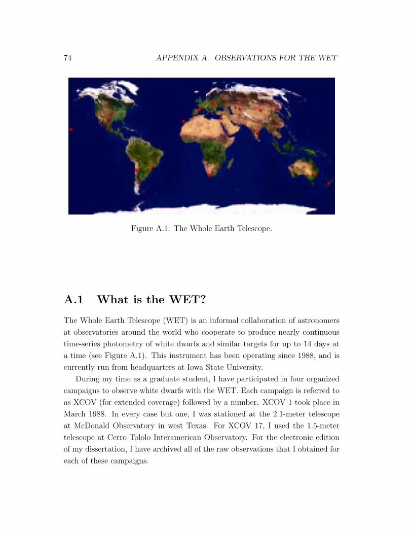
74 APPENDIX A. OBSERVATIONS FOR THE WET
Figure A.1: The Whole Earth Telescope.
A.1 What is the WET?
The Whole Earth Telescope (WET) is an informal collaboration of astronomers
at observatories around the world who cooperate to produce nearly continuous
time-series photometry of white dwarfs and similar targets for up to 14 days at
a time (see Figure A.1). This instrument has been operating since 1988, and is
currently run from headquarters at Iowa State University.
During my time as a graduate student, I have participated in four organized
campaigns to observe white dwarfs with the WET. Each campaign is referred to
as XCOV (for extended coverage) followed by a number. XCOV 1 took place in
March 1988. In every case but one, I was stationed at the 2.1-meter telescope
at McDonald Observatory in west Texas. For XCOV 17, I used the 1.5-meter
telescope at Cerro Tololo Interamerican Observatory. For the electronic edition
of my dissertation, I have archived all of the raw observations that I obtained for
each of these campaigns.
A.2. XCOV 15: DQ HERCULIS 75
A.2 XCOV 15: DQ Herculis
archive in digital dissertation:[tsm-0023 → tsm-0032]
A.3 XCOV 17: BPM 37093
archive in digital dissertation:[tsm-0033 → tsm-0048]
A.4 XCOV 18: HL Tau 76
archive in digital dissertation:[tsm-0049 → tsm-0072]
A.5 XCOV 19: GD 358
archive in digital dissertation:[tsm-0074 → tsm-0085]

76 APPENDIX A. OBSERVATIONS FOR THE WET
Appendix B
Interactive Simulations
77
78 APPENDIX B. INTERACTIVE SIMULATIONS
B.1 Pulsation Visualizations
In digital dissertation: Spherical harmonic visualizations.
B.2 The Effect of Viewing Angle
In digital dissertation: Interactive demonstration of the effect of viewing angle
on the amplitude of the observed brightness variations.
Appendix C
Computer Codes
79
80 APPENDIX C. COMPUTER CODES
This appendix contains an archive of the source code for the software that I have
used for the calculations presented in this dissertation.
EVOLVE.F is a streamlined version of the White Dwarf Evolution Code
(WDEC) described in §4.3.2 with references to its origins and to the sources
of data for the input physics. WDEC takes as input a hot starter model with a
specific mass, which can come from detailed evolutionary calculations in the case
of DOV stars, or from a simple polytropic approximation in the case of DBV and
DAV stars. Using this starter model and other parameters specified in the header,
WDEC adds an envelope with the specified composition and fractional mass and
evolves the model quasi-statically until it reaches the specified temperature.
PULSATE.F uses the final output model produced by WDEC and calculates
the m = 0 adiabatic non-radial oscillation periods of a specified spherical degree
(`) within a specified period range. The periods resulting from the adiabatic
approximation typically differ from the non-adiabatic results by only a few thou-
sandths of a second, which is well below the present level of observational noise.
PVM FITNESS.F is the code that uses the message-passing routines of the
Parallel Virtual Machine (PVM) software to allow the public-domain genetic al-
gorithm PIKAIA to evaluate the fitnesses of trials in parallel rather than sequen-
tially. This code automatically determines the number of processors available for
the calculation, balances the load when machines with differing speeds are used,
and works around crashed jobs in a sensible way.
FF SLAVE.F is an interface between the parallel genetic algorithm and the
streamlined version of WDEC. This code runs on each machine that is used to
calculate white dwarf models. It uses the message-passing routines of PVM to re-
ceive sets of parameters from the master process, evaluates the white dwarf model
specified by those parameters, compares the model periods to the observations,
and returns a measure of fitness to PIKAIA.
The practical aspects of running the evolution and pulsation codes are ad-
dressed in the documentation archive at the end of this appendix.
C.1. EVOLVE.F 81
C.1 EVOLVE.F
In digital dissertation: Hypertext version of evolution code.
C.2 PULSATE.F
In digital dissertation: Hypertext version of pulsation code.
82 APPENDIX C. COMPUTER CODES
C.3 PVM FITNESS.F
subroutine pvm_fitness (slave, num_jobs, npar, oldph, fitness)
c ---------------------------------------------
c parallel fitness evaluation using PVM
c ---------------------------------------------
implicit none
c
include ’../include/fpvm3.h’
c
integer job, info, nhost, msgtype, iwhich, i
integer mytid, dtid, tids(0:128), flag, ntask
integer ttids(64), ptids(64), htids(64), flags(64)
integer speed, narch, numt, npar, nspawn, last, wait
integer num_jobs, ndone, length, par, trial, listen
integer finished(1024),resubmitted(1024)
c
double precision result, data(64)
real fitness(1024), oldph(64,1024)
c
character*40 hostname
character*18 host
character*8 slave, arch
character*8 aout(64)
c ---------------------------------------------
c initialize book-keeping variables
c ---------------------------------------------
listen = 0
wait = 0
ndone = 0
do job=1,num_jobs
finished(job) = 0
resubmitted(job) = 0
enddo
C.3. PVM FITNESS.F 83
c ---------------------------------------------
c enroll this program in PVM
c ---------------------------------------------
call pvmfmytid( mytid )
call pvmfconfig( nhost, narch, dtid, host, arch, speed, info )
c ---------------------------------------------
c run jobs on slave nodes only
c ---------------------------------------------
arch = ’.’
flag = PvmTaskHost+PvmHostCompl
nspawn = nhost-1
call pvmfspawn( slave, flag, arch, nspawn, tids, numt )
c ---------------------------------------------
c check for problems spawning slaves
c ---------------------------------------------
if( numt .lt. nspawn ) then
write(*,*) ’trouble spawning ’,slave
write(*,*) ’ Check tids for error code’
call shutdown( numt, tids )
endif
c
write(*,*)
c ---------------------------------------------
c send an initial job to each node
c ---------------------------------------------
do job=0,nspawn-1
c
trial = job + 1
do par=1,npar
data(par) = INT((100*oldph(par,trial))+0.5)/100.
enddo
c
call pvmfinitsend( PVMDEFAULT, info )
call pvmfpack( INTEGER4, trial, 1, 1, info )
call pvmfpack( INTEGER4, npar, 1, 1, info )
84 APPENDIX C. COMPUTER CODES
call pvmfpack( REAL8, data, npar, 1, info )
msgtype = 1
call pvmfsend( tids(job), msgtype, info )
c
11 format("job ",i3,3(2x,f4.2))
write(*,11) trial,data(1),data(2),data(3)
c
enddo
c
write(*,*)
c
do job=1,num_jobs
c ---------------------------------------------
c listen for responses
c ---------------------------------------------
25 msgtype = 2
call pvmfnrecv( -1, msgtype, info )
listen = listen + 1
c
if (info .GT. 0) then
write(*,*) "<-- job ",job
listen = 0
wait = 0
c ---------------------------------------------
c get data from responding node
c ---------------------------------------------
call pvmfunpack( INTEGER4, trial, 1, 1, info )
call pvmfunpack( REAL8, result, 1, 1, info )
call pvmfunpack( INTEGER4, length, 1, 1, info )
call pvmfunpack( STRING, hostname, length, 1, info )
c ---------------------------------------------
c re-send jobs that return crash signal
c ---------------------------------------------
if ((result .eq. 0.0).and.(resubmitted(trial).ne.1)) then
write(*,*) "detected fitness=0 job: trial ",trial
C.3. PVM FITNESS.F 85
call sendjob
& (trial,hostname,’ffrslave’,npar,resubmitted,oldph)
goto 25
endif
c
fitness(trial) = result
finished(trial) = 1
ndone = ndone + 1
c
33 format(i4,2x,i4,2x,a8,2x,3(f4.2,2x),f12.8)
write(*,33) ndone,trial,hostname,oldph(1,trial),
& oldph(2,trial),oldph(3,trial),result
c ---------------------------------------------
c send new job to responding node
c ---------------------------------------------
140 if (ndone .LE. (num_jobs-nspawn)) then
trial = job + nspawn
call sendjob
& (trial,hostname,slave,npar,resubmitted,oldph)
endif
goto 100
endif
c ---------------------------------------------
c re-submit crashed jobs to free nodes
c ---------------------------------------------
if (ndone .GT.(num_jobs-nspawn)) then
last = ndone-nspawn
if (ndone .GE.(num_jobs-5)) last=ndone
do trial=1,last
if ((finished(trial).NE.1).AND.
& (resubmitted(trial).NE.1).AND.(wait.NE.1)) then
write(*,*) "detected crashed job: trial ",trial
call sendjob
& (trial,hostname,’ffrslave’,npar,resubmitted,oldph)
wait = 1
86 APPENDIX C. COMPUTER CODES
goto 25
endif
enddo
endif
c ---------------------------------------------
c return to listen again or move on
c ---------------------------------------------
if ((info .EQ. 0).AND.(listen .LT. 10000000)) goto 25
c
write(*,*) "detected unstable jobs: setting fitness=0"
do trial=1,num_jobs
if ((finished(trial) .NE. 1).AND.
& (resubmitted(trial) .EQ. 1)) then
fitness(trial) = 0.0
finished(trial) = 1
ndone = ndone + 1
write(*,33) ndone,trial,hostname,oldph(1,trial),
& oldph(2,trial),oldph(3,trial),fitness(trial)
endif
enddo
goto 199
100 continue
enddo
c ---------------------------------------------
c kill any remaining jobs
c ---------------------------------------------
199 iwhich = PVMDEFAULT
call pvmftasks( iwhich, ntask, ttids(1), ptids(1),
& htids(1), flags(1), aout(1), info )
do i=2,ntask
call pvmftasks( iwhich, ntask, ttids(i), ptids(i),
& htids(i), flags(i), aout(i), info )
if ((aout(i) .EQ. ’ff_slave’).OR.
& (aout(i) .EQ. ’ffrslave’)) then
call pvmfkill (ttids(i), info)
C.3. PVM FITNESS.F 87
endif
enddo
c
call pvmfexit(info)
c
return
end
c**********************************************************************
subroutine sendjob(trial,hostname,slave,npar,resubmitted,oldph)
c
implicit none
c
include ’../include/fpvm3.h’
c
integer tids(0:128), numt, msgtype, par, npar, trial, info, flag
integer resubmitted(1024)
c
double precision data(64)
real oldph(64,1024)
c
character*40 hostname
character*8 slave
c
call pvmfspawn( slave, 1, hostname, 1, tids, numt )
c
if ( numt .lt. 1 ) then
write(*,*) ’trouble spawning’,slave
write(*,*) ’ Check tids for error code’
call shutdown( numt, tids )
endif
c
do par=1,npar
data(par) = INT((100*oldph(par,trial))+0.5)/100.
enddo
c
88 APPENDIX C. COMPUTER CODES
call pvmfinitsend( PVMDEFAULT, info )
call pvmfpack( INTEGER4, trial, 1, 1, info )
call pvmfpack( INTEGER4, npar, 1, 1, info )
call pvmfpack( REAL8, data, npar, 1, info )
msgtype = 1
call pvmfsend( tids(0), msgtype, info )
c
55 format("job --> ",a8,3(2x,f4.2))
write(*,55) hostname,data(1),data(2),data(3)
c
if (slave .EQ. ’ffrslave’) resubmitted(trial) = 1
c
return
end
c**********************************************************************
subroutine shutdown( nproc, tids )
c
implicit none
c
integer nproc, i, info, tids(*)
c
do i=0, nproc
call pvmfkill( tids(i), info )
enddo
c
call pvmfexit( info )
c
return
end
c**********************************************************************
C.4. FF SLAVE.F 89
C.4 FF SLAVE.F
program ff_slave
c ---------------------------------------------
c fitness function slave program
c ---------------------------------------------
implicit none
c
include ’../include/fpvm3.h’
c
integer info, mytid, mtid, msgtype, speed, length, i
integer n, nhost, narch, dtid, hostid, trial
c
double precision ff, data(32), result
c
character*40 hostname,machine,arch
c ---------------------------------------------
c enroll this program in PVM
c ---------------------------------------------
call pvmfmytid( mytid )
c ---------------------------------------------
c get the master’s task id
c ---------------------------------------------
call pvmfparent( mtid )
c ---------------------------------------------
c receive data from master host
c ---------------------------------------------
msgtype = 1
call pvmfrecv( mtid, msgtype, info )
call pvmfunpack( INTEGER4, trial, 1, 1, info )
call pvmfunpack( INTEGER4, n, 1, 1, info )
call pvmfunpack( REAL8, data, n, 1, info )
c ---------------------------------------------
c perform calculations with data
c ---------------------------------------------
90 APPENDIX C. COMPUTER CODES
result = ff( n, data )
c ---------------------------------------------
c send result to master host
c ---------------------------------------------
call pvmftidtohost( mytid, hostid )
100 call pvmfconfig( nhost, narch, dtid, hostname, arch, speed, info )
if (dtid .ne. hostid) goto 100
length = len(hostname)
machine = hostname(1:length)
c
call pvmfinitsend( PVMDEFAULT, info )
call pvmfpack( INTEGER4, trial, 1, 1, info )
call pvmfpack( REAL8, result, 1, 1, info )
call pvmfpack( INTEGER4, length, 1, 1, info )
call pvmfpack( STRING, machine, length, 1, info )
msgtype = 2
call pvmfsend( mtid, msgtype, info )
c ---------------------------------------------
c leave PVM before exiting
c ---------------------------------------------
call pvmfexit(info)
c
stop
end
c*********************************************************************
C.5. DOCUMENTATION 91
C.5 Documentation
In digital dissertation: Documentation archive.
• evolution code: (PS/PDF)
• prep code: (PS/PDF)
• pulsation code: (PS/PDF)

92 APPENDIX C. COMPUTER CODES
Bibliography
Arcoragi, J. & Fontaine, G. 1980, ApJ, 242, 1208
Beauchamp, A., Wesemael, F., Bergeron, P., Fontaine, G., Saffer, R. A., Liebert,
J. & Brassard, P. 1999, ApJ, 516, 887
Becker, D., Sterling, T., Savarese, D., Dorband, J., Ranawak, U., & Packer, C.
1995, in Proceedings of the International Conference on Parallel Processing
(New York: Institute of Electrical and Electronics Engineers).
Bern, K. & Wramdemark, S. 1973, Lowell Obs. Bull., No. 161
Bohm, K. H. & Cassinelli, J. 1971, A&A, 12, 21
Bradley, P. A. 1993, Ph.D. thesis, University of Texas-Austin
Bradley, P. A. & Winget, D. E. 1994a, ApJ, 421, 236
Bradley, P. A. & Winget, D. E. 1994b, ApJ, 430, 850
Bradley, P. A., Winget, D. E. & Wood, M. A. 1993, ApJ, 406, 661
Brassard, P., Fontaine, G., Wesemael, F. & Hansen, C. J. 1992, ApJS, 80, 369
Buchmann, L. 1996, ApJ, 468, L127
Caughlan, G. R., Fowler, W. A., Harris, M. J., & Zimmerman, B. A. 1985,
Atomic Data and Nuclear Data Tables, 32, 197
Charbonneau, P. 1995, ApJS, 101, 309
Charbonneau, P., Tomczyk, S., Schou, J., Thompson, M.J. 1998, ApJ, 496, 1015
93
94 BIBLIOGRAPHY
Crick, F. 1984, quoted by Daniel C. Dennett in Elbow Room: the varieties of
free will worth wanting (Cambridge, MA: MIT Press)
Darwin, C. 1859, The Origin of Species (New York: Penguin Books)
Dehner, B. T. & Kawaler, S. D. 1995, ApJ, 445, L141
Feynman, R. P., Leighton, R. B. & Sands, M. 1963, The Feynman Lectures on
Physics, Vol. 1 (Reading, MA: Addison-Wesley)
Fontaine, G., Graboske, H. C., Jr., & Van Horn, H. M. 1977, ApJS, 35, 293
Fowler, W. A. 1986, in Highlights of Modern Physics, ed. S. L. Shapiro & S. A.
Teukolsky (New York: John Wiley & Sons), 3
Geist, A., Beguelin, A., Dongarra, J., Jiang, W., Manchek, R., & Sunderam,
V. 1994, PVM: Parallel Virtual Machine, A Users’ Guide and Tutorial for
Networked Parallel Computing, (Cambridge: MIT Press)
Goldberg, D. 1989, Genetic Algorithms in Search, Optimization, and Machine
Learning, (Reading, MA: Addison-Wesley).
Gottbrath, C. et al. 1999, http://arxiv.org/abs/astro-ph/9912202
Greenstein, J. L. 1969, ApJ, 158, 281
Hakala, P. 1995, A&A, 296, 164
Harrington, R. S., Kallarakal, V. V., Christy, J. W., Dahn, C. C., Riepe, B. Y.,
Guetter, H. H., Ables, H. D., Hewitt, A. V., Vrba, F. J., & Walker, R. L. 1985,
AJ, 90, 123
Hoeflich, P., Wheeler, J. C., & Thielemann, F. K. 1998, ApJ, 495, 617
Iglesias, C. A., & Rogers, F. J. 1993, ApJ, 412, 752
Itoh, N., Hayashi, H., Nishikawa, A., & Kohyama, Y. 1996, ApJS, 102, 411
Kallrath, J. & Linnell, A. P. 1987, ApJ, 313, 346
BIBLIOGRAPHY 95
Kanaan, A., Kepler, S. O., Giovannini, O., & Diaz, M. 1992, ApJ, 390, L89
Kanaan, A., Nitta-Kleinman, A., Winget, D. E., Kepler, S. O., Montgomery, M.,
& WET team 2000, Baltic Astronomy, 9, 87
Kawaler, S. 1986, Ph.D. thesis, University of Texas-Austin
Kawaler, S. D. 1990, ASP Conf. Ser. 11: Confrontation Between Stellar Pulsation
and Evolution, 494
Kawaler, S. &Weiss, P. 1990, in Proc. Oji International Seminar, Progress of Seis-
mology of the Sun and Stars, ed. Y. Osaki & H. Shibahashi (Berlin: Springer),
431
Kennelly, E. J., Walker, G. A. H., Catala, C., Foing, B. H., Huang, L., Jiang,
S., Hao, J., Zhai, D., Zhao, F., Neff, J. E., Houdebine, E. R., Ghosh, K. K.,
Charbonneau, P. 1996, A&A, 313, 571.
Kleinman, S. J., Nather, R. E., Winget, D. E., Clemens, J. C., Bradley, P. A.,
Kanaan, A., Provencal, J. L., Claver, C. F., Watson, T. K., Yanagida, K.,
Nitta, A., Dixson, J. S., Wood, M. A., Grauer, A. D., Hine, B. P., Fontaine,
G., Liebert, J., Sullivan, D. J., Wickramasinghe, D. T., Achilleos, N., Marar,
T. M. K., Seetha, S., Ashoka, B. N., Meistas, E., Leibowitz, E. M., Moskalik,
P., Krzesinski, J., Solheim, J. -., Bruvold, A., O’Donoghue, D., Kurtz, D. W.,
Warner, B., Martinez, P., Vauclair, G., Dolez, N., Chevreton, M., Barstow, M.
A., Kepler, S. O., Giovannini, O., Augusteijn, T., Hansen, C. J., & Kawaler,
S. D. 1998, ApJ, 495, 424
Kutter, G. S. & Savedoff, M. P. 1969, ApJ, 156, 1021
Lamb, D. Q. 1974, Ph.D. thesis, University of Rochester
Lamb, D. Q. & Van Horn, H. M. 1975, ApJ, 200, 306
Lang, M. 1995, Ir. Astron. J., 22, 167
Lazio, T. 1997, PASP, 109, 1068
Metcalfe, T. S. 1999, AJ, 117, 2503
96 BIBLIOGRAPHY
Metcalfe, T. S., & Nather, R. E. 1999, Linux Journal, 65, 58
Metcalfe, T. S., & Nather, R. E. 2000, Baltic Astronomy, 9, 479
Metcalfe, T. S., Nather, R. E. & Winget, D. E. 2000, ApJ, 545, 974
Montgomery, M. H. 1998, Ph.D. thesis, University of Texas-Austin
Montgomery, M. H., Klumpe, E. W., Winget, D. E., & Wood, M. A. 1999, ApJ,
525, 482
Montgomery, M. H., Metcalfe, T. S. & Winget, D. E. 2001, ApJ, 548, L53
Montgomery, M. H. & Winget, D. E. 1999, ApJ, 526, 976
Napiwotzki, R., Green, P. J. & Saffer, R. A. 1999, ApJ, 517, 399
Nather, R. E., Winget, D. E., Clemens, J. C., Hansen, C. J. & Hine, B. P. 1990,
ApJ, 361, 309
Nitta, A., Kanaan, A., Kepler, S. O., Koester, D., Montgomery, M. H., & Winget,
D. E. 2000, Baltic Astronomy, 9, 97
Proctor, D. D. & Linnell, A. P. 1972, ApJS, 24, 449
Proust, M. 1981, in Readers Digest, 24 February (Pleasantville, NY: The Reader’s
Digest Association, Inc.)
Provencal, J. L., Shipman, H. L., Thejll, P., & Vennes, S. 2000, ApJ, 542, 1041
Salaris, M., Dominguez, I., Garcia-Berro, E., Hernanz, M., Isern, J. &
Mochkovitch, R. 1997, ApJ, 486, 413
Shaw, G. B. 1903, Man and Superman; a comedy and a philosophy (Westminster:
A. Constable)
Sweigart, A., Greggio, L. & Renzini, A. 1990, ApJ, 364, 527
Tassoul, M., Fontaine, G., & Winget, D. E. 1990, ApJS, 72, 335
BIBLIOGRAPHY 97
Torvalds, L. 1999, interview on CNN & Fortune, 24 February
(http://digistar.com/luclist/1999-02/0032.html)
Vuille, F., O’Donoghue, D., Buckley, D. A. H., Massacand, C. -., Solheim, J. E.,
Bard, S., Vauclair, G., Giovannini, O., Kepler, S. O., Kanaan, A., Provencal, J.
L., Wood, M. A., Clemens, J. C., Kleinman, S. J., O’Brien, M. S., Nather, R.
E., Winget, D. E., Nitta, A., Klumpe, E. W., Montgomery, M. H., Watson, T.
K., Bradley, P. A., Sullivan, D. J., Wu, K., Marar, T. M. K., Seetha, S., Ashoka,
B. N., Mahra, H. S., Bhat, B. C., Babu, V. C., Leibowitz, E. M., Hemar, S.,
Ibbetson, P., Mashals, E., Meistas, E., Moskalik, P., ZoÃla, S., Krzesinski, J., &
Pajdosz, G. 2000, MNRAS, 314, 689
Wahde, M. 1998, A&AS, 132, 417
Wampler, J. 1973, quoted by Ed Nather in 1995, Baltic Astronomy, 4, 124
Wegner, G. 1979, in IAU Colloquium 53, White Dwarfs and Variable Degenerate
Stars (Rochester, New York: University of Rochester), 250
Winget, D. E. 1981, Ph.D. thesis, University of Rochester
Winget, D. E., Robinson, E. L., Nather, R. D. & Fontaine, G. 1982, ApJ, 262,
L11
Winget, D. E., Nather, R. E., Clemens, J. C., Provencal, J. L., Kleinman, S. J.,
Bradley, P. A., Claver, C. F., Dixson, J. S., Montgomery, M. H., Hansen, C.
J., Hine, B. P., Birch, P., Candy, M., Marar, T. M. K., Seetha, S., Ashoka, B.
N., Leibowitz, E. M., O’Donoghue, D., Warner, B., Buckley, D. A. H., Tripe,
P., Vauclair, G., Dolez, N., Chevreton, M., Serre, T., Garrido, R., Kepler, S.
O., Kanaan, A., Augusteijn, T., Wood, M. A., Bergeron, P., & Grauer, A. D.
1994, ApJ, 430, 839
Winget, D. E., Nather, R. E., Clemens, J. C., Provencal, J., Kleinman, S. J.,
Bradley, P. A., Wood, M. A., Claver, C. F., Frueh, M. L., Grauer, A. D.,
Hine, B. P., Hansen, C. J., Fontaine, G., Achilleos, N., Wickramasinghe, D.
T., Marar, T. M. K., Seetha, S., Ashoka, B. N., O’Donoghue, D., Warner, B.,
Kurtz, D. W., Buckley, D. A., Brickhill, J., Vauclair, G., Dolez, N., Chevreton,
98 BIBLIOGRAPHY
M., Barstow, M. A., Solheim, J. E., Kanaan, A., Kepler, S. O., Henry, G. W.,
& Kawaler, S. D. 1991, ApJ, 378, 326
Wood, M. 1990, Ph.D. thesis, University of Texas-Austin
Woosley, S. E., Timmes, F. X. & Weaver, T. A. 1993, in Nuclei in the Cosmos,
Vol. 2, ed. F. Kappeler & K. Wisshak (Philadelphia: IOP), 531
Vita
Travis Scott Metcalfe was born in Seaside, Oregon on 12 October 1973. He lived
on the central Oregon coast with his parents Jerry and Karen until graduating
from Newport High School in 1991. In August of that year, he moved to Tucson,
Arizona to study Astronomy and Physics at the University of Arizona, where he
received a Bachelor of Science degree in May 1996. He came to Austin, Texas in
August 1996 to begin graduate studies in the Department of Astronomy at the
University of Texas where he received a Master of Arts degree two years later.
Permanent Address: 3013 Harris Park Avenue, Austin, Texas 78705
This dissertation was typeset by the author.
99