Copula functions

Advanced Methods of Risk Management

Umberto Cherubini

Copula functions

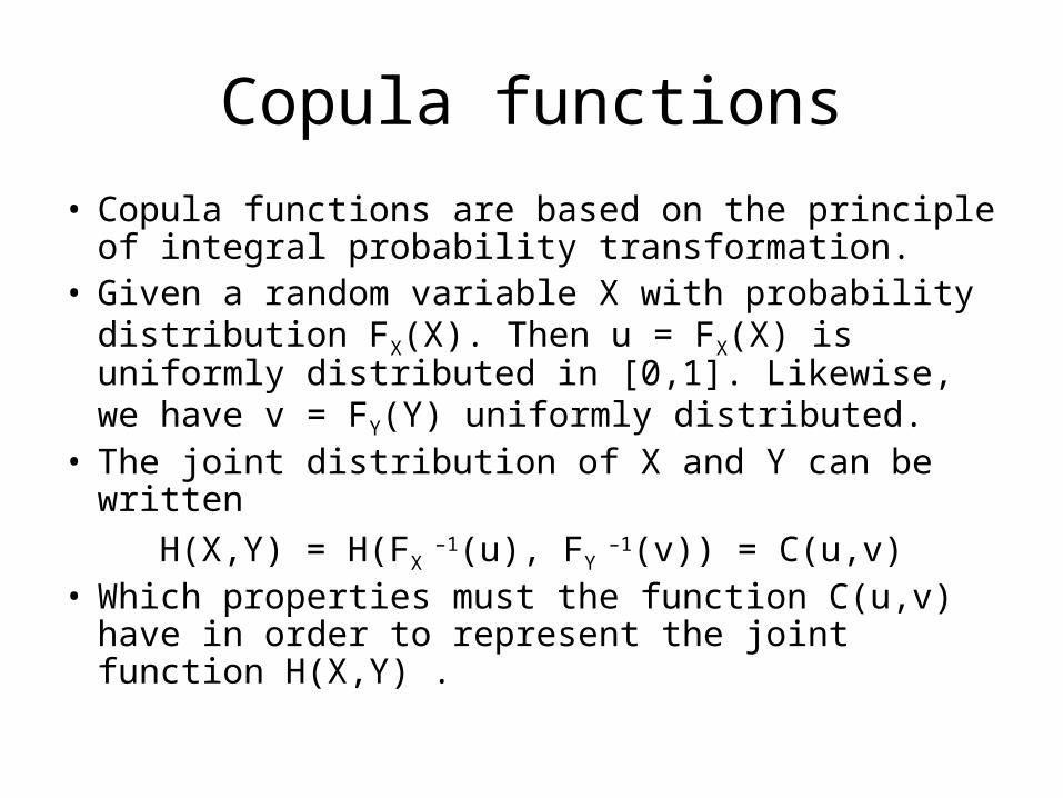
• Copula functions are based on the principle of integral probability transformation.

• Given a random variable X with probability distribution FX(X). Then u = FX(X) is uniformly distributed in [0,1]. Likewise, we have v = FY(Y) uniformly distributed.

• The joint distribution of X and Y can be written

H(X,Y) = H(FX –1(u), FY

–1(v)) = C(u,v)• Which properties must the function C(u,v) have

in order to represent the joint function H(X,Y) .

Copula function Mathematics

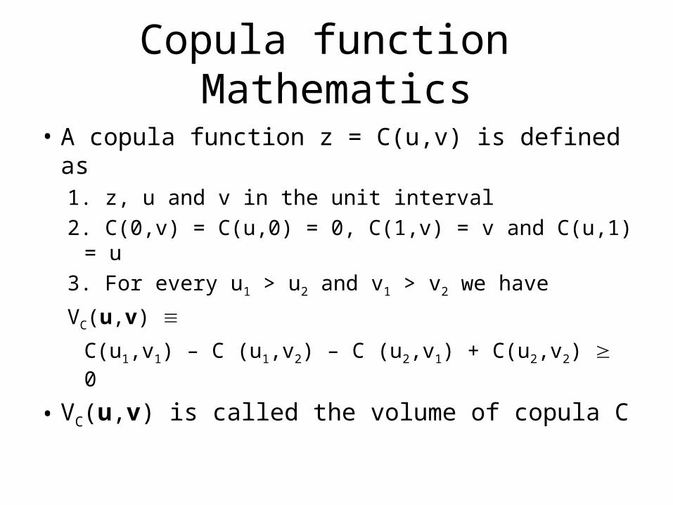
• A copula function z = C(u,v) is defined as1. z, u and v in the unit interval

2. C(0,v) = C(u,0) = 0, C(1,v) = v and C(u,1) = u

3. For every u1 > u2 and v1 > v2 we have

VC(u,v)

C(u1,v1) – C (u1,v2) – C (u2,v1) + C(u2,v2) 0

• VC(u,v) is called the volume of copula C

Copula functions: Statistics

• Sklar theorem: each joint distribution H(X,Y) can be written as a copula function C(FX,FY) taking the marginal distributions as arguments, and vice versa, every copula function taking univariate distributions as arguments yields a joint distribution.

Copula function and dependence structure

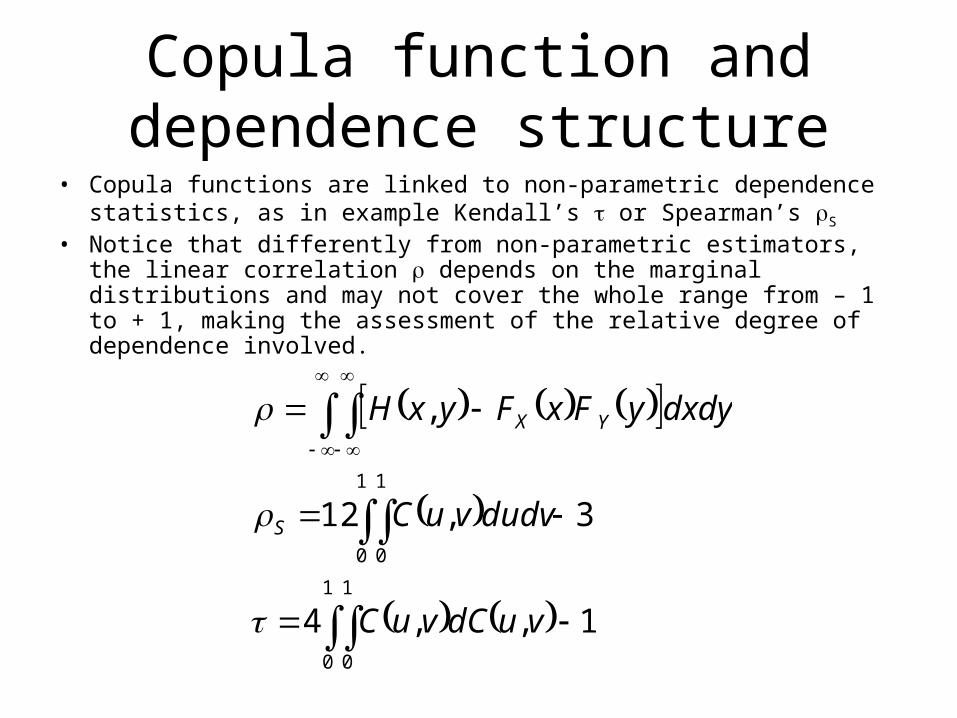
• Copula functions are linked to non-parametric dependence statistics, as in example Kendall’s or Spearman’s S

• Notice that differently from non-parametric estimators, the linear correlation depends on the marginal distributions and may not cover the whole range from – 1 to + 1, making the assessment of the relative degree of dependence involved.

1,,4

3,12

,

1

0

1

0

1

0

1

0

vudCvuC

dudvvuC

dxdyyFxFyxH

S

YX

Dualities among copulas

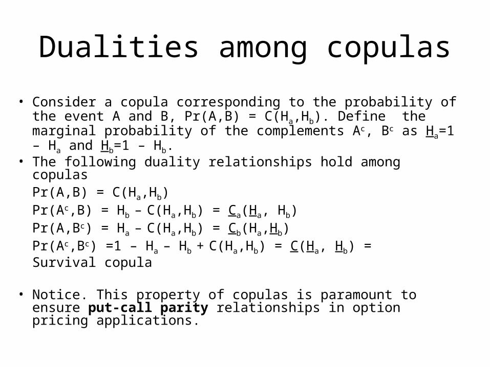
• Consider a copula corresponding to the probability of the event A and B, Pr(A,B) = C(Ha,Hb). Define the marginal probability of the complements Ac, Bc as Ha=1 – Ha and Hb=1 – Hb.

• The following duality relationships hold among copulasPr(A,B) = C(Ha,Hb)Pr(Ac,B) = Hb – C(Ha,Hb) = Ca(Ha, Hb)Pr(A,Bc) = Ha – C(Ha,Hb) = Cb(Ha,Hb)Pr(Ac,Bc) =1 – Ha – Hb + C(Ha,Hb) = C(Ha, Hb) =

Survival copula

• Notice. This property of copulas is paramount to ensure put-call parity relationships in option pricing applications.

Radial symmetry

• Take a copula function C(u,v) and its survival version

C(1 – u, 1 – v) = 1 – v – u + C( u, v)

• A copula is said to be endowed with the radial symmetry (reflection symmetry) property if

C(u,v) = C(u, v)

AND/OR operators

• Copula theory also features more tools, which are seldom mentioned in financial applications.

• Example: Co-copula = 1 – C(u,v)

Dual of a Copula = u + v – C(u,v)• Meaning: while copula functions represent

the AND operator, the functions above correspond to the OR operator.

Conditional probability I

• The dualities above may be used to recover the conditional probability of the events.

v

vuC

vH

vHuHvHuH

b

baba

,

Pr

,PrPr

Conditional probability II

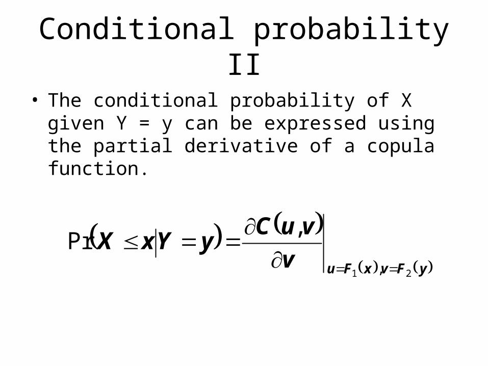
• The conditional probability of X given Y = y can be expressed using the partial derivative of a copula function.

yFvxFuv

vuCyYxX

21 ,

,Pr

Tail dependence in crashes…

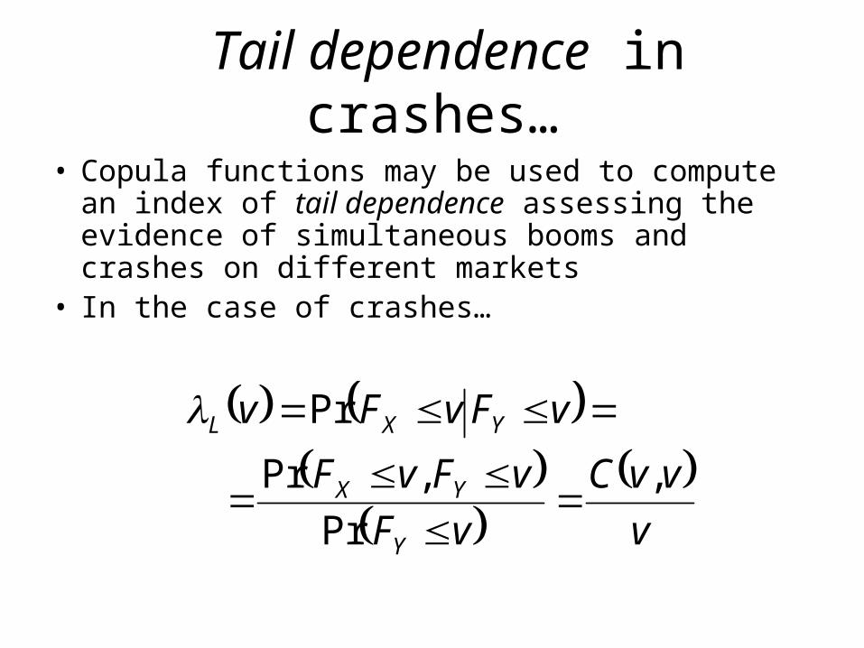
• Copula functions may be used to compute an index of tail dependence assessing the evidence of simultaneous booms and crashes on different markets

• In the case of crashes…

v

vvC

vF

vFvF

vFvFv

Y

YX

YXL

,

Pr

,Pr

Pr

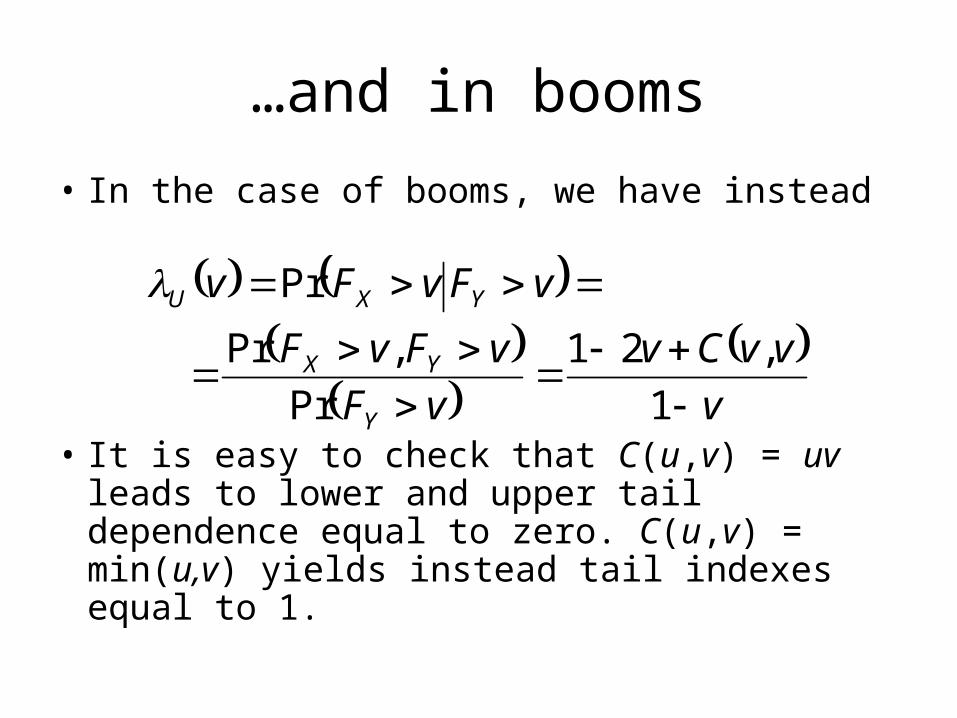
…and in booms

• In the case of booms, we have instead

• It is easy to check that C(u,v) = uv leads to lower and upper tail dependence equal to zero. C(u,v) = min(u,v) yields instead tail indexes equal to 1.

v

vvCv

vF

vFvF

vFvFv

Y

YX

YXU

1

,21

Pr

,Pr

Pr

The Fréchet family

• C(x,y) =Cmin +(1 – – )Cind + Cmax , , [0,1] Cmin= max (x + y – 1,0), Cind= xy, Cmax= min(x,y)

• The parameters ,are linked to non-parametric dependence measures by particularly simple analytical formulas. For example

S = • Mixture copulas (Li, 2000) are a particular case in

which copula is a linear combination of Cmax and Cind for positive dependent risks (>0, Cmin and Cind for the negative dependent (>0,

Elliptical copulas• Ellictal multivariate distributions, such as multivariate

normal or Student t, can be used as copula functions.• Normal copulas are obtained

C(u1,… un ) =

= N(N – 1 (u1 ), N – 1 (u2 ), …, N – 1 (uN ); ) and extreme events are indipendent.

• For Student t copula functions with v degrees of freedom C (u1,… un ) =

= T(T – 1 (u1 ), T – 1 (u2 ), …, T – 1 (uN ); , v) extreme events are dependent, and the tail dependence index is a function of v.

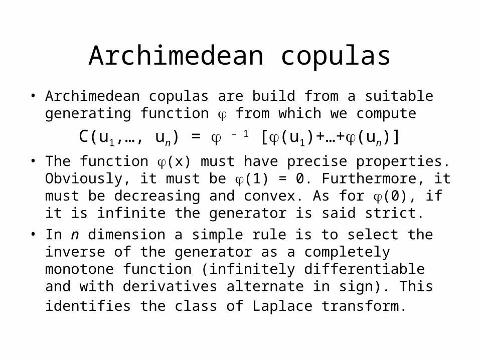
Archimedean copulas• Archimedean copulas are build from a suitable

generating function from which we compute

C(u1,…, un) = – 1 [(u1)+…+(un)]• The function (x) must have precise properties.

Obviously, it must be (1) = 0. Furthermore, it must be decreasing and convex. As for (0), if it is infinite the generator is said strict.

• In n dimension a simple rule is to select the inverse of the generator as a completely monotone function (infinitely differentiable and with derivatives alternate in sign). This identifies the class of Laplace transform.

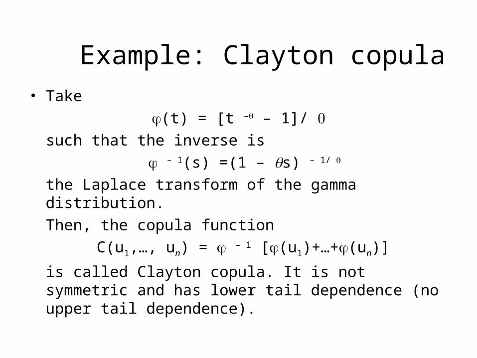
Example: Clayton copula• Take

(t) = [t – – 1]/ such that the inverse is

– 1(s) =(1 – s) – 1/

the Laplace transform of the gamma distribution.

Then, the copula function

C(u1,…, un) = – 1 [(u1)+…+(un)]

is called Clayton copula. It is not symmetric and has lower tail dependence (no upper tail dependence).

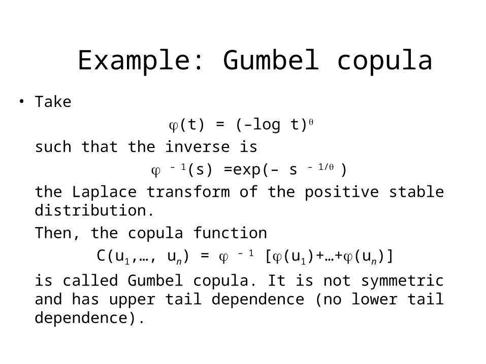
Example: Gumbel copula• Take

(t) = (–log t)

such that the inverse is

– 1(s) =exp(– s – 1/ )

the Laplace transform of the positive stable distribution.

Then, the copula function

C(u1,…, un) = – 1 [(u1)+…+(un)]

is called Gumbel copula. It is not symmetric and has upper tail dependence (no lower tail dependence).

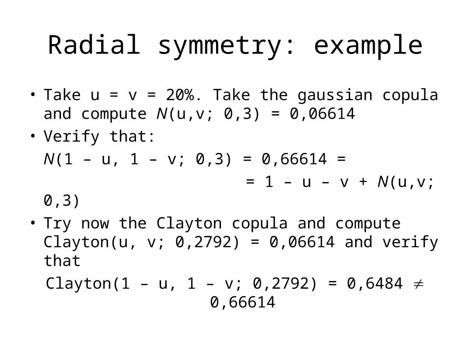
Radial symmetry: example

• Take u = v = 20%. Take the gaussian copula and compute N(u,v; 0,3) = 0,06614

• Verify that:

N(1 – u, 1 – v; 0,3) = 0,66614 =

= 1 – u – v + N(u,v; 0,3)• Try now the Clayton copula and compute

Clayton(u, v; 0,2792) = 0,06614 and verify that

Clayton(1 – u, 1 – v; 0,2792) = 0,6484 0,66614

Kendall function

• For the class of Archimedean copulas, there is a multivariate version of the probability integral transfomation theorem.

• The probability t = C(u,v) is distributed according to the distribution

KC (t) = t – (t)/ ’(t)where ’(t) is the derivative of the generating function. There exist extensions of the Kendall function to n dimensions.

• Constructing the empirical version of the Kendall function enables to test the goodness of fit of a copula function (Genest and McKay, 1986).

Kendall function: Clayton copula

0

0,2

0,4

0,6

0,8

1

1,2

0 0,1 0,2 0,3 0,4 0,5 0,6 0,7 0,8 0,9 1

Copula product

• The product of a copula has been defined (Darsow, Nguyen and Olsen, 1992) as

A*B(u,v)

and it may be proved that it is also a copula.

1

0

,,dt

t

vtB

t

tuA

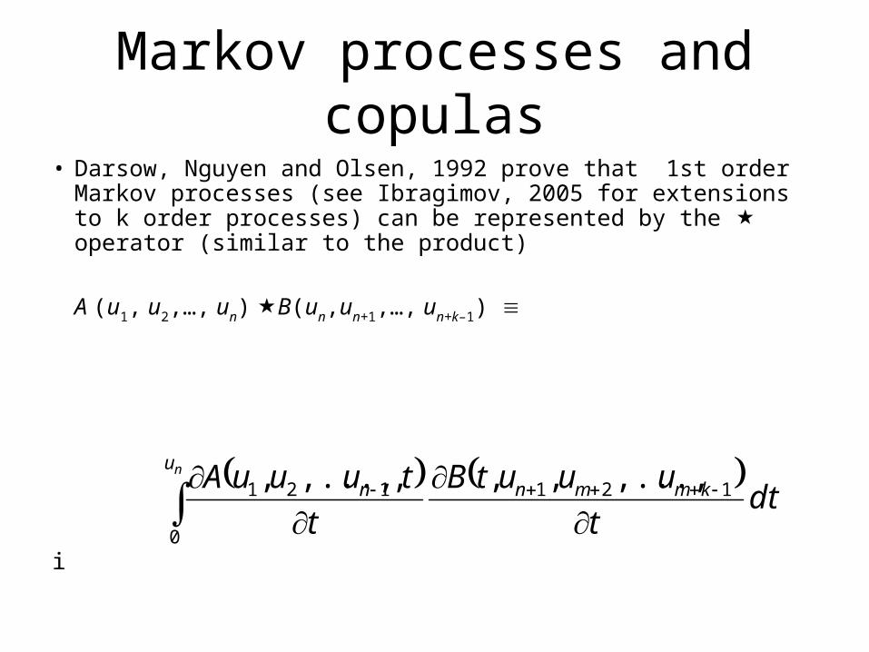
Markov processes and copulas

• Darsow, Nguyen and Olsen, 1992 prove that 1st order Markov processes (see Ibragimov, 2005 for extensions to k order processes) can be represented by the operator (similar to the product)

A (u1, u2,…, un) B(un,un+1,…, un+k–1)

i

nu

kmmnn dtt

uuutB

t

tuuuA

0

121121 ,...,,,,,...,,

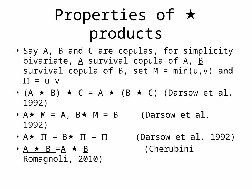
Properties of products

• Say A, B and C are copulas, for simplicity bivariate, A survival copula of A, B survival copula of B, set M = min(u,v) and = u v

• (A B) C = A (B C) (Darsow et al. 1992)• A M = A, B M = B (Darsow et al. 1992)• A = B = (Darsow et al.

1992)• A B =A B (Cherubini Romagnoli,

2010)

Symmetric Markov processes

• Definition. A Markov process is symmetric if

1. Marginal distributions are symmetric

2. The product

T1,2(u1, u2) T2,3(u2,u3)… Tj – 1,j(uj –1 , uj)

is radially symmetric • Theorem. A B is radially simmetric if either i)

A and B are radially symmetric, or ii) A B = A A with A exchangeable and A survival copula of A.

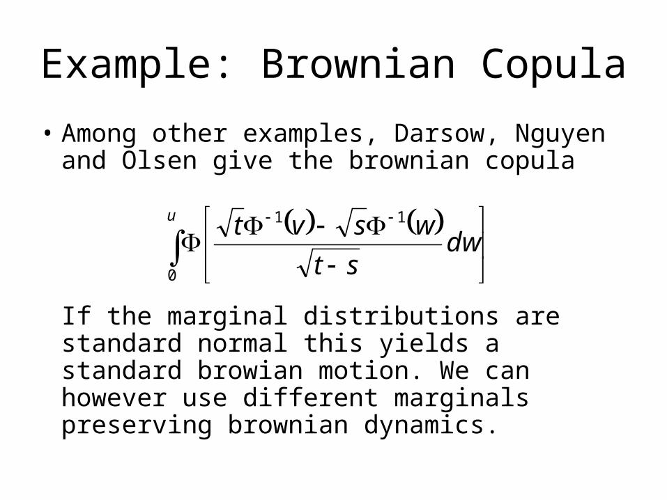
Example: Brownian Copula

• Among other examples, Darsow, Nguyen and Olsen give the brownian copula

If the marginal distributions are standard normal this yields a standard browian motion. We can however use different marginals preserving brownian dynamics.

u

dwst

wsvt

0

11

Basic credit risk applications

• Guarantee: assume a client has default probability 20% and he asks for guarantee from a guarantor with default probability of 1%. What is the default probability of the loan?

• First to default: you buy protection on a first to default on a basket of “names”. What is the price? Are you long or short correlation?

• Last to default: you buy protection on the last default in a basket of “names”. What is the price? Are you long or short correlation?

An example: guarantee on credit

• Assume a credit exposure with probability of default of Ha = 20% in a year.

• Say the credit exposure is guaranteed by another party with default probability equal to Ha = 1% .

• The probability of default on the exposure is now the joint probability

DP = C(Ha , Hb)

• The worst case is perfect dependence between default of the two counterparties leading to

DP = min(Ha , Hb )

“First-to-default” derivatives• Consider a credit derivative, that is a contract

providing “protection” the first time that an element in the basket of obligsations defaults. Assume the protection is extended up to time T.

• The value of the derivative is FTD = LGD v(t,T)(1 – Q(0))

• Q(0) is the survival probability of all the names in the basket:

Q(0) Q(1 > T, 2 > T…)