Copula-basierte räumliche Interpolation - BOKU · Copula-basierte r aumliche Interpolation ......
53
Copula-basierte r ¨ aumliche Interpolation J¨ urgen Pilz 1 und Hannes Kazianka 1 1 Alpen-Adria-University Klagenfurt, Department of Statistics, Austria Herbsttagung “R in Ausbildung, Forschung und Anwendung 1.10. – 3.10.2009, Bad Doberan
Transcript of Copula-basierte räumliche Interpolation - BOKU · Copula-basierte r aumliche Interpolation ......

Copula-basierte raumlicheInterpolation
Jurgen Pilz1 und Hannes Kazianka1
1Alpen-Adria-University Klagenfurt, Department of Statistics, Austria
Herbsttagung “R in Ausbildung, Forschung und Anwendung1.10. – 3.10.2009, Bad Doberan

Preliminary remarks Kriging Matern Prediction Bayesian Extension I Extension II: Spatial Modelling Using Copulas Applications R-Software
Outline
1 Preliminary remarks
2 Spatial linear model/Kriging
3 Matern class of covariance functions
4 Prediction using likelihood methods
5 Bayesian approach
6 Extension I: Bayesian trans-GaussianPrediction
7 Extension II: Spatial Modelling Using CopulasParameter Estimation
8 Applications
9 R-Software

Preliminary remarks Kriging Matern Prediction Bayesian Extension I Extension II: Spatial Modelling Using Copulas Applications R-Software
Preliminary Remarks
Geostatistics
(much more than Kriging methodology!) has spread from traditional areas ofapplication (mining and oil exploration) to nearly all branches of bio, earth andenvironmental sciences, medicine and technology
Recent Areas of Application:
Public Health + Epidemiology
Precision Farming
Image Analysis (Gibbs/Markov-RF)
Statistical Process Control (Semiconductor industry)
Telecommunication network design
Partial Convergence with Machine Learning methodology

Preliminary remarks Kriging Matern Prediction Bayesian Extension I Extension II: Spatial Modelling Using Copulas Applications R-Software
Geostatistics
= Statistical analysis of random phenomena distributed in space (and time)using the theory of Random Functions (Random Fields)
Milestone-Books
during the last 15 years:
1993: N. Cressie: Statistics for Spatial Data. Rev. ed., Wiley
1997: P. Goovaerts: Geostatistics for Natural Resources Evaluation.Oxford Univ. Press
1999: M.L. Stein: Interpolation of Spatial Data. Some Theory forKriging. Springer

Preliminary remarks Kriging Matern Prediction Bayesian Extension I Extension II: Spatial Modelling Using Copulas Applications R-Software
1999: J.-P. Chiles & P. Delfiner: Geostatistics: Modeling SpatialUncertainty. Wiley
1999: R. Olea: Geostatistics for Engineers and Earth Scientists. Springer
2003: H. Wackernagel: Multivariate Geostatistics. 3rd ed., Springer
2003: S. Banerjee, B.P. Carlin & A. Gelfand: Hierarchical Modeling andAnalysis for Spatial Data. CRC Chapman & Hall
2007: R. Webster & M. A. Oliver: Geostatistics for EnvironmentalScientists. 2nd ed., Wiley
2007: P.J. Diggle & P.J. Ribeiro, P.J.: Model-based Geostatistics.Springer

Preliminary remarks Kriging Matern Prediction Bayesian Extension I Extension II: Spatial Modelling Using Copulas Applications R-Software
Most recent books:
R. Bivand, E. Pebesma and V. Gomez-Rubio: Applied Spatial DataAnalysis with R. Springer 2008
J. Pilz (Ed.): Interfacing Geostatistics and GIS. Springer 2009
Current research issues:
Non-Gaussianity
Non-stationarity (Direct modeling via kernels, Grid deformation)
Spatio-temporal extensions (Space-time covariance functions)
Spatio-temporal monitoring network design/design of computerexperiments

Preliminary remarks Kriging Matern Prediction Bayesian Extension I Extension II: Spatial Modelling Using Copulas Applications R-Software
Spatial linear model/Kriging
Z(x) = m(x) + ε(x); x ∈ D ⊂ Rd , d > 1Data = Trend + Error
Linear trend model:
(1)m(x) = E{Z(x)|β, θ} = f (x)Tβ↙ ↘
Trend parameter covariance parameter
e.g. polynomials: m(x1, x2) = β0 + β1x1 + β2x2
(2)Cov{(Z(x1),Z(x2))|β, θ} = Cθ(x1 − x2)
covariance stationarity
(1) + (2) = universal kriging setup

Preliminary remarks Kriging Matern Prediction Bayesian Extension I Extension II: Spatial Modelling Using Copulas Applications R-Software
Given:
observations at points x1, . . . , xn ∈ D
Z = (Z(x1), . . . ,Z(xn))T observation vector
Goal:
Prediction of Z(x0) at x0 ∈ D,i.e. choose Z(x0) such that
E{Z(x0)− Z(x0)}2 −→ MinZ
Spatial BLUP
ZUK (x) = λT Ztakes the formZUK (x0) = f (x0)T β + c(x0)TK−1 (Z− F β)| {z }
↓ ↓GLS of β residual vector

Preliminary remarks Kriging Matern Prediction Bayesian Extension I Extension II: Spatial Modelling Using Copulas Applications R-Software
where
F = (f (x1), . . . , f (xn))T = design matrix
c(x0) = (Cov(Z(x0),Z(xi )))i=1,...,n
K = (Cov(Z(xi ),Z(xj)))i,j=1,...,n
= covariance matrix of Z
Usually,
further assumptions likeisotropy: Cθ(x1 − x2) = Cθ(||x1 − x2||)sparse parametrization: θ = (θ1, θ2, θ3)
= (nugget, sill, range)

Preliminary remarks Kriging Matern Prediction Bayesian Extension I Extension II: Spatial Modelling Using Copulas Applications R-Software
statistical / numerical problem:
non-linearity in θ (esp. in range)
Weak point
of kriging: BLUP-optimality rests on exact knowledge of covariance function.In practice however: plug-in-kriging using empirical moment estimator of thecov. function, which is then fitted to some (conditionally) pos. semidefinitefunction
For sensible
predictions: further assumptions about the law of the R.F. are required. Localbehaviour of the R.F. is critical

Preliminary remarks Kriging Matern Prediction Bayesian Extension I Extension II: Spatial Modelling Using Copulas Applications R-Software
Essential Property:
Mean square differentiability(defined as an L2-limit)
Result:
Z is m-times m.s.d. iff |C (2m)(0)| <∞; (m = 1, 2, . . .)Local behaviour of W.R.F.’s is best studied using spectral methods
Bochner’s Theorem:
C(·) is cov. function for a w.m.s.c. R.F. on Rd ←→
C(x) =
ZRd
exp(iωT x) F (dω)
↓positive finite measure= spectral measure
⇒ Spectral density & Covariance function form a Fourier pair

Preliminary remarks Kriging Matern Prediction Bayesian Extension I Extension II: Spatial Modelling Using Copulas Applications R-Software
Matern class of covariance functions
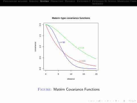
Matern class
of covariance functions widely popular over the last 10 years:
Cθ(h) = c ∗ (α|h|)νKν(α|h|)
Kν = modified Bessel function of order νθ = (c, α, ν) = (sill, scale, smoothness) ∈ (0,∞)3
Spectral density: fM(ω) = c(α2 + ω2)−ν−d/2
valid for isotropic R.F.s in any dimension d!
Fitting procedures in: geoR, geoRglm (Diggle& Ribeiro, 2007)
Preliminary remarks Kriging Matern Prediction Bayesian Extension I Extension II: Spatial Modelling Using Copulas Applications R-Software
0 5 10 15 20
0.0
0.5
1.0
1.5
2.0
Matern−type covariance functions
distance
cova
rianc
e ν = 50
ν = 0.5
ν = 1.5
Figure: Matern Covariance Functions
Preliminary remarks Kriging Matern Prediction Bayesian Extension I Extension II: Spatial Modelling Using Copulas Applications R-Software
Prediction using likelihood methods
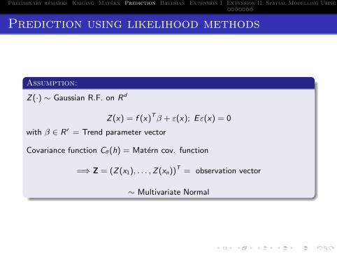
Assumption:
Z(·) ∼ Gaussian R.F. on Rd
Z(x) = f (x)Tβ + ε(x); Eε(x) = 0
with β ∈ R r = Trend parameter vector
Covariance function Cθ(h) = Matern cov. function
=⇒ Z = (Z(x1), . . . ,Z(xn))T = observation vector
∼ Multivariate Normal

Preliminary remarks Kriging Matern Prediction Bayesian Extension I Extension II: Spatial Modelling Using Copulas Applications R-Software
Log-Likelihood-Function
l(β, θ) = − n2
log(2π)− 12
log detK(θ)
− 12(Z− Fβ)TK(θ)−1(Z− Fβ)
For any given θ, l(·, θ) is maximized by
β(θ) = [FTK(θ)−1F ]−1FTK(θ)−1Z
↙ ↘ ↙design matrix covariance matrix
Problem:
Maximize l(β(θ), θ) w.r. to θ||
profile log-likelihood for θ

Preliminary remarks Kriging Matern Prediction Bayesian Extension I Extension II: Spatial Modelling Using Copulas Applications R-Software
Disadvantage:
MLE of θ tends to underestimate the variation
Adjustments for the bias not available
Extension:
non-Gaussian R.F.sNeed models / computational methods for calculating likelihood functionsDiggle, Tawn & Moyeed (1998): MCMC methods
Key:
Model-based Geostatistics⇒ serious computational issues!

Preliminary remarks Kriging Matern Prediction Bayesian Extension I Extension II: Spatial Modelling Using Copulas Applications R-Software
Bayesian approach
Advantage:
provides a general methodology for taking into account the uncertainty aboutparameters on subsequent predictions.Especially important for the Matern class:Large uncertainty about ν, it is impossible to obtain defensible MSE’s from thedata without incorporating prior information about ν!
First versions of Bayesian Kriging:Kitanidis (1986), Omre (1987)

Preliminary remarks Kriging Matern Prediction Bayesian Extension I Extension II: Spatial Modelling Using Copulas Applications R-Software
Bayesian solution:
For making inferences about Z(x0) =: Z0, use the predictive density p(Z0|Z)given the data Z = (Z(x1), . . . ,Z(xn))T ,
p(Z0|Z) =
ZΘ
ZB
p(Z0|β, θ,Z)p(β, θ|Z)dβdθ
↓ ↓trend parameter covariance par.
(1st order par.) (2nd order par.)
where p(β, θ|Z) = posterior density
=p(Z|β, θ)p(β, θ)R
Θ
RB
p(Z|β, θ)p(β, θ)dβdθ
∝ likelihood f. ∗ prior d.

Preliminary remarks Kriging Matern Prediction Bayesian Extension I Extension II: Spatial Modelling Using Copulas Applications R-Software
Proposal:
conditional simulation
p(β, θ|Z) ∝ p(Z|θ, β)| {z }likelihood f.
∗p(β) ∗ p(θ|Z)| {z }simulation
Empirical Bayes approach, see Pilz & Spock, SERRA (2008)
Alternative way:
Objective Bayesian analysis:determine non-informative priorsBerger, Sanso, DeOliveira 2001

Preliminary remarks Kriging Matern Prediction Bayesian Extension I Extension II: Spatial Modelling Using Copulas Applications R-Software
Extension I: Bayesian trans-GaussianPrediction
The transformed Gaussian Model
Observations from random field {Z(x), x ∈ X ⊂ Rm}.Box-Cox family of power transformations (Box and Cox, 1964)
gλ(z) =
zλ−1λ
: λ 6= 0log(z) : λ = 0
transforms the random field Z(x) for some unknown parameter λ to aGaussian one with unknown trend and unknown covariance functionCθ(x1, x2).
Definition of prior:
Θ = (λ, θ)
p(β,Θ) = p(β, λ, θ)

Preliminary remarks Kriging Matern Prediction Bayesian Extension I Extension II: Spatial Modelling Using Copulas Applications R-Software
Likelihood:
p(Z0,Zdat|β,Θ) =
p(gλ(Z0,Zdat)|β, λ, θ, σ2)| {z }normal
∗ Jλ(Z0,Zdat)| {z }Jacobian
Generalization:
arbitrary monotone transformations g(z), e.g. g(z) = log(− log(1− z))
Posterior Predictive Distribution:
p(Z0|Zdat) =
ZΘ
p(Z0|Zdat,Θ)| {z }Gaussian
p(Θ|Zdat)| {z }?
dΘ,
Solution
Instead of specifying the prior we specify the posterior p(Θ|Zdat) bymeans of a parametric bootstrap of some estimator of Θ.

Preliminary remarks Kriging Matern Prediction Bayesian Extension I Extension II: Spatial Modelling Using Copulas Applications R-Software
0 5 10 15 20 25 30 350
5
10
15
20
25
30
35
40Histogram of Gomel data
Figure: Histogram of Gomel data

Preliminary remarks Kriging Matern Prediction Bayesian Extension I Extension II: Spatial Modelling Using Copulas Applications R-Software
−2.5 −2 −1.5 −1 −0.5 0 0.5 1 1.5 2 2.5
−2
−1.5
−1
−0.5
0
0.5
1
1.5
2
posterior of anisotropy axes
Figure: Bootstrapped anisotropy axes

Preliminary remarks Kriging Matern Prediction Bayesian Extension I Extension II: Spatial Modelling Using Copulas Applications R-Software
Advantages
Complete probability distribution (not only kriged values + variances)
We have median, quantiles a.s.o.
−→ threshold values, confidence intervals a.s.o.
“Automatic” Bayes procedure

Preliminary remarks Kriging Matern Prediction Bayesian Extension I Extension II: Spatial Modelling Using Copulas Applications R-Software
0 10 20 30 40 50 60 70 80 90 1000
0.005
0.01
0.015
0.02
0.025
0.03
0.035
0.04(x,y)=(134.7458,27.9661)
Figure: Posterior predictive distribution at (x,y)=(134.7,27.9)

Preliminary remarks Kriging Matern Prediction Bayesian Extension I Extension II: Spatial Modelling Using Copulas Applications R-Software
q0.95
−100 −50 0 50 100
−100
−80
−60
−40
−20
0
20
40
60
80
100
5
10
15
20
25
30
35
40
45
50
Figure: 95% posterior predictive quantile

Preliminary remarks Kriging Matern Prediction Bayesian Extension I Extension II: Spatial Modelling Using Copulas Applications R-Software
mean
−100 −50 0 50 100
−100
−80
−60
−40
−20
0
20
40
60
80
100
0
5
10
15
20
25
Figure: posterior predictive mean

Preliminary remarks Kriging Matern Prediction Bayesian Extension I Extension II: Spatial Modelling Using Copulas Applications R-Software
standard deviation
−100 −50 0 50 100
−100
−80
−60
−40
−20
0
20
40
60
80
100
2
4
6
8
10
12
14
Figure: posterior predictive standard deviation

Preliminary remarks Kriging Matern Prediction Bayesian Extension I Extension II: Spatial Modelling Using Copulas Applications R-Software
treshold 8
−100 −50 0 50 100
−100
−80
−60
−40
−20
0
20
40
60
80
100
0
0.1
0.2
0.3
0.4
0.5
0.6
0.7
0.8
Figure: probability to be above threshold 8.0

Preliminary remarks Kriging Matern Prediction Bayesian Extension I Extension II: Spatial Modelling Using Copulas Applications R-Software
0 10 20 30 40 50 60 70 80 900
10
20
30
40
50
60
70
80
90(cross)validation
percent actual data above threshold
expe
cted
per
cent
dat
a ab
ove
thre
shol
d
Figure: predicted percentage versus actual percentage of data abovethreshold

Preliminary remarks Kriging Matern Prediction Bayesian Extension I Extension II: Spatial Modelling Using Copulas Applications R-Software
Extension II: Spatial Modelling Using Copulas
Problem:
What can we do if data are extreme, highly skewed?
Answer:
Copula-based spatial modeling
Copulas
are distribution functions on the unit cube [0, 1]n
Sklar’s TheoremLet H be an n-dimensional distribution function with margins F1, . . . ,Fn. Thenthere exists an n-dimensional copula C such that for all x = (x1, . . . , xn) ∈ Rn
H (x1, . . . , xn) = C (F1 (x1) , . . . ,Fn (xn))
If F1, . . . ,Fn are all continuous, then C is unique. Conversely, it holds:
C (u1, . . . , un) = H“F−1
1 (u1) , . . . ,F−1n (un)
”.

Preliminary remarks Kriging Matern Prediction Bayesian Extension I Extension II: Spatial Modelling Using Copulas Applications R-Software
Properties of Copulas
Copulas describe the dependence between the quantiles of randomvariables. They describe dependence without information about marginaldistributions.
Copulas are invariant under strictly increasing transformations of therandom variables. Frequently applied data transformations do not changethe copula.
Random variables X1, . . . ,Xn are stochastically independent if and only iftheir copula is the product copula Πn (u) =
Qni=1 ui .
Bivariate copulas are directly related to the Spearman-ρ correlationcoefficient:
ρ(X1,X2) = 12
1Z0
1Z0
C(u1, u2)du1du2 − 3

Preliminary remarks Kriging Matern Prediction Bayesian Extension I Extension II: Spatial Modelling Using Copulas Applications R-Software
Copulas in Geostatistics
How to incorporate copulas into the geostatistical framework?The copula becomes a function of the separating vector h and does not dependon the location (due to the stationarity). The dependence of any two locationsseparated by the vector h is described by
P (Z (x) ≤ z1,Z (x + h) ≤ z2) = Ch (FZ (z1) ,FZ (z2)) ,
where FZ is the univariate distribution of the random process and is assumed tobe the same for each location x. (Bardossy, 2006)
It is advantageous to work with copulas constructed from elliptical distributionssince the correlation matrix explicitly appears in their analytical expression andcan be parameterized by a correlation function model.

Preliminary remarks Kriging Matern Prediction Bayesian Extension I Extension II: Spatial Modelling Using Copulas Applications R-Software
Examples
Gaussian Copula: C (u1, . . . , un) = Φ0,Σ
`Φ−1 (u1) , . . . ,Φ−1 (un)
´.
χ2-copula (Bardossy)
Preliminary remarks Kriging Matern Prediction Bayesian Extension I Extension II: Spatial Modelling Using Copulas Applications R-Software
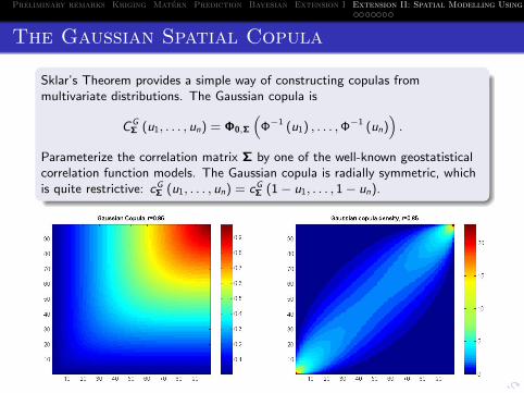
The Gaussian Spatial Copula
Sklar’s Theorem provides a simple way of constructing copulas frommultivariate distributions. The Gaussian copula is
CGΣ (u1, . . . , un) = Φ0,Σ
“Φ−1 (u1) , . . . ,Φ−1 (un)
”.
Parameterize the correlation matrix Σ by one of the well-known geostatisticalcorrelation function models. The Gaussian copula is radially symmetric, whichis quite restrictive: cG
Σ (u1, . . . , un) = cGΣ (1− u1, . . . , 1− un).
Preliminary remarks Kriging Matern Prediction Bayesian Extension I Extension II: Spatial Modelling Using Copulas Applications R-Software
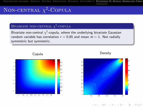
Non-central χ2-Copula
Bivariate non-central χ2-copula
Bivariate non-central χ2-copula, where the underlying bivariate Gaussianrandom variable has correlation r = 0.85 and mean m = 1. Not radiallysymmetric but symmetric.
Copula Density

Preliminary remarks Kriging Matern Prediction Bayesian Extension I Extension II: Spatial Modelling Using Copulas Applications R-Software
Parameter Estimation for Cont. Marginals
Maximum Likelihood
Let Θ = (θ,λ) be the parameter vector, where θ are the correlation function(and anisotropy) parameters and λ are the parameters of the known family ofunivariate distributions F .
l (Θ; Z (x1) , . . . ,Z (xn)) =
cθ (Fλ (Z (x1)) , . . . ,Fλ (Z (xn)))nY
i=1
fλ (Z (xi ))

Preliminary remarks Kriging Matern Prediction Bayesian Extension I Extension II: Spatial Modelling Using Copulas Applications R-Software
Model-Based Approach
Plug-In Estimator
We use the predictive distribution in the rank space. Taking theML-estimations, Θ, as the true values we arrive at the plug-in estimator
z (x0) = E“z (x0) | z (x1) , . . . , z (xn) , Θ
”.
The estimator can therefore be obtained as
z (x0) =
Z 1
0
F−1λ (u (x0))| {z }Jacobian
cθ (u (x0) | u (x1) , . . . , u (xn))| {z }conditional copula
du (x0) .
Not difficult with Gaussian copula

Preliminary remarks Kriging Matern Prediction Bayesian Extension I Extension II: Spatial Modelling Using Copulas Applications R-Software
Equivalence
The trans-Gaussian kriging model using any strictly monotone transformation isequivalent to the Gaussian spatial copula model.
Proof follows from the invariance under strictly increasing transformations andthe radial-symmetry of the Gaussian distribution.

Preliminary remarks Kriging Matern Prediction Bayesian Extension I Extension II: Spatial Modelling Using Copulas Applications R-Software
Advantages of copula Kriging
Any other copula different from the Gaussian copula can be used whichleads to a generalization of trans-Gaussian kriging
Even if we stay within the Gaussian framework, it is simpler to specify afamily of marginal distributions than to determine a suitabletransformation function, especially for multi-modal and extreme-valuedata
Full predictive distribution is available and can be used to calculatepredictive quantiles, confidence regions and prediction variance
Easily extendable to a Bayesian approach
Shares properties with kriging such as being exact at known locations
Incorporating covariates is easy to do

Preliminary remarks Kriging Matern Prediction Bayesian Extension I Extension II: Spatial Modelling Using Copulas Applications R-Software
EC-STREP “INTAMAP” (Interoperability and AutomaticMapping)
Main objective of this project (IST, FP6): develop an interoperableframework for real time automatic mapping of critical environmentalvariables by extending spatial statistical methods and employing open,web-based, data exchange and visualisation tools.
Project includes partners from Austria, Germany, Netherlands, Italy, GreatBritain and Greece, for further information see
www.intamap.org
Main application:
System for automated mapping of radiation levels reported by 30 Europeancountries participating in
EURDEP = European Radiological Data Exchange Platform
Data availability in nearly real-time (more and more on an hourly basis)currently: > 4200 stations

Preliminary remarks Kriging Matern Prediction Bayesian Extension I Extension II: Spatial Modelling Using Copulas Applications R-Software
EURDEP Data Flow

Preliminary remarks Kriging Matern Prediction Bayesian Extension I Extension II: Spatial Modelling Using Copulas Applications R-Software
An overview
of the achievements of the INTAMAP-Project, including prototypedemonstration + specific workshops by the project partners, was given at
Int. StatGIS 2009 Conference,“Geoinformatics for Environmental Surveillance”Milos, Greece, June 17-19, 2009
Preliminary remarks Kriging Matern Prediction Bayesian Extension I Extension II: Spatial Modelling Using Copulas Applications R-Software
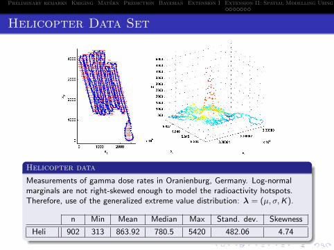
Helicopter Data Set
Helicopter data
Measurements of gamma dose rates in Oranienburg, Germany. Log-normalmarginals are not right-skewed enough to model the radioactivity hotspots.Therefore, use of the generalized extreme value distribution: λ = (µ, σ,K).
n Min Mean Median Max Stand. dev. Skewness
Heli 902 313 863.92 780.5 5420 482.06 4.74

Preliminary remarks Kriging Matern Prediction Bayesian Extension I Extension II: Spatial Modelling Using Copulas Applications R-Software
Analysis of Helicopter Data I
Analysis using the copula-based approach
The Gaussian spatial copula is used
Geometric anisotropy is considered
Correlation function model is chosen to be a Matern model including anugget effect: ϑ1, ϑ2, κ
Parameter point estimates are obtained using maximum likelihood

Preliminary remarks Kriging Matern Prediction Bayesian Extension I Extension II: Spatial Modelling Using Copulas Applications R-Software
Analysis of Helicopter Data II
Preliminary remarks Kriging Matern Prediction Bayesian Extension I Extension II: Spatial Modelling Using Copulas Applications R-Software
Analysis of Helicopter Data III
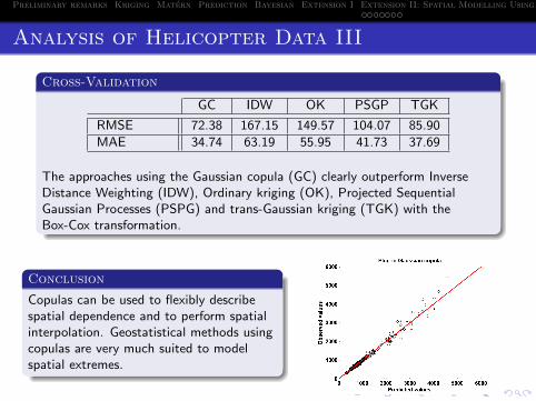
Cross-Validation
GC IDW OK PSGP TGK
RMSE 72.38 167.15 149.57 104.07 85.90
MAE 34.74 63.19 55.95 41.73 37.69
The approaches using the Gaussian copula (GC) clearly outperform InverseDistance Weighting (IDW), Ordinary kriging (OK), Projected SequentialGaussian Processes (PSPG) and trans-Gaussian kriging (TGK) with theBox-Cox transformation.
Conclusion
Copulas can be used to flexibly describespatial dependence and to perform spatialinterpolation. Geostatistical methods usingcopulas are very much suited to modelspatial extremes.

Preliminary remarks Kriging Matern Prediction Bayesian Extension I Extension II: Spatial Modelling Using Copulas Applications R-Software
Software I
Main properties of the R-Software
Code for estimation of parameters and prediction at unobserved locationsin the case of the Gaussian spatial copula model and the non-centralχ2-copula model with continuous marginals is part of the intamap
R-library. It is freely available fromhttps://sourceforge.net/projects/intamap.
Automatic choice of marginal distribution, correlation function model,anisotropy and starting values by using certain heuristics.
Additionally, the intamap library performs
Inverse Distance Weighting (library gstat),Ordinary Kriging (library gstat),Projected Sequential Gaussian Processes (library psgp),Trans-Gaussian Kriging (library gstat).
The intamap package will be also available from CRAN soon.

Preliminary remarks Kriging Matern Prediction Bayesian Extension I Extension II: Spatial Modelling Using Copulas Applications R-Software
Software II
Commands
There are two main functions, estimateParameters.copula andspatialPredict.copula, that perform parameter estimation and spatialprediction for an intamapObject of the class copula.
intamapObject<-createIntamapObject(observations=observations,
predictionLocations=predictionLocations,class="copula")
It is possible to work with trend surface models by setting the argumentformulaString of the intamapObject accordingly. The requested predictiontypes are defined by the argument outputWhat:
outputWhat = list(mean = TRUE, variance = FALSE, excProb = 10,
excprob = 20, quantile = 0.025, quantile = 0.975)
The user has the choice to specify the correlation function model, anisotropyand starting values of the optimization himself or to let the program choosethem.

Preliminary remarks Kriging Matern Prediction Bayesian Extension I Extension II: Spatial Modelling Using Copulas Applications R-Software
Software III
The interpolate-Function
The interpolate function of the intamap R-package is designed for automaticspatial modeling and interpolation. The function decides which of the followingthree interpolation methods to apply: automap (ordinary kriging asimplemented in the R-package automap), psgp and copula. If copula ischosen
1 the function estimateAnisotropy decides whether to include geometricanisotropy into the analysis or not,
2 autofitVariogram of the automap R-library is used to select a correlationmodel and starting parameters for the corresponding parameters,
3 the Gaussian, the log-Gaussian, the Student-t, the generalized extremevalue (GEV) and the logistic distribution are tested and the best fittingone is chosen,
4 the Gaussian copula is used.
Preliminary remarks Kriging Matern Prediction Bayesian Extension I Extension II: Spatial Modelling Using Copulas Applications R-Software
Software IV
Computation Time
Computation time is a major issue for the spatial copula algorithms. Thefollowing will influence the computational load:
The number of observations.
For the non-central χ2-copula model computation will take much longersince a composite-likelihood approach is used.
If the Matern model is chosen, the algorithm will be slower because thebesselk function needs to be evaluated and there is one additionalparameter.
If the GEV distribution is chosen, the algorithm will be slower becausethere are three parameters to optimize instead of only two.
Additionally accounting for covariates slows down the estimation process,since regression parameters are introduced and need to be optimized.
Prediction is slower when quantiles of the predictive distribution arerequested. This is because an integral equation is solved numerically.
“Good” initial values for the optimization reduce the computational loadsince fewer iterations are needed to reach convergence.

Preliminary remarks Kriging Matern Prediction Bayesian Extension I Extension II: Spatial Modelling Using Copulas Applications R-Software
H. Kazianka and J. Pilz.
Bayesian spatial modeling and interpolation using copulas.
In D. Hristopoulos, editor, StatGIS 2009, Chania, 2009. TechnicalUniversity of Crete.
H. Kazianka and J. Pilz.
Bayesian spatial modeling and interpolation using copulas.
Computers and Geosciences, Special issue on “GeoInformatics forenvironmental surveillance” (submitted), 2009.
H. Kazianka and J. Pilz.
Copula-based geostatistical modeling of continuous and discrete dataincluding covariates.
Stochastic Environmental Research and Risk Assessment, (in press), 2009.
H. Kazianka and J. Pilz.
Spatial interpolation using copula-based geostatistical models.
In P. Atkinson and C. Lloyd, editors, GeoENV VII - Geostatistics forEnvironmental Applications. Springer, Berlin, 2009.
H. Kazianka, G. Spock, and J. Pilz.
Modeling and interpolation of non-Gaussian spatial data: a comparativestudy.

Preliminary remarks Kriging Matern Prediction Bayesian Extension I Extension II: Spatial Modelling Using Copulas Applications R-Software
In D. Hristopoulos, editor, StatGIS 2009, Chania, 2009. TechnicalUniversity of Crete.
J. Pilz, H. Kazianka, and G. Spock.
Interoperability - Spatial interpolation and automated mapping.
In T. Tsiligiridis, editor, Proceedings of the 4th International Conferenceon Information and Communication Technologies in Bio and EarchSciences HAICTA 2008, pages 110–118, Athens, 2008. AgriculturalUniversity of Athens.
G. Spock, H. Kazianka, and J. Pilz.
Bayesian trans-Gaussian kriging with log-log transformed skew data.
In J. Pilz, editor, Interfacing Geostatistics and GIS, pages 29–44. Springer,Berlin, 2009.