
Coordination of distance and overcurrent relays using a ... Labrador.pdf · vii Abstract...
138
Center for Technology and Urbanism Department of Electrical Engineering Angel Labrador Coordination of distance and overcurrent relays using a mathematical optimization technique A dissertation submitted to the Electrical Engineering Graduate Program at the State University of Londrina in fulfillment of the requirements for the degree of MASTER OF SCIENCE in Electrical Engineering. Londrina 2018
Transcript of Coordination of distance and overcurrent relays using a ... Labrador.pdf · vii Abstract...

Center for Technology and Urbanism
Department of Electrical Engineering
Angel Labrador
Coordination of distance and overcurrentrelays using a mathematical optimization
technique
A dissertation submitted to the ElectricalEngineering Graduate Program at the StateUniversity of Londrina in fulfillment of therequirements for the degree of MASTER OFSCIENCE in Electrical Engineering.
Londrina
2018

i
Angel Labrador
Coordination of distance and overcurrent relays using amathematical optimization technique
A dissertation submitted to the ElectricalEngineering Graduate Program at the StateUniversity of Londrina in fulfillment of therequirements for the degree of MASTER OFSCIENCE in Electrical Engineering.Subjet area: Power Systems
Supervisor:Professor Ph.D. Luis Alfonso Gallego Pareja
Londrina
2018

Bibliography card
Labrador, AngelCoordination of distance and overcurrent relays using a mathematical optimization
technique. Londrina, 2018. 114 p.
Dissertation (Master) – State University of Londrina, PR, BR.Deparment of Electrical Engineering
1 Optimization techniques 2 Power system protection 3 Overcurrent relay coordi-nation 4 Distance relay coordination 5 Mixed protection scheme 6 Heuristic algorithm

iii
Angel Labrador
Coordination of distance and overcurrent relays using amathematical optimization technique
A dissertation submitted to the ElectricalEngineering Graduate Program at the StateUniversity of Londrina in fulfillment of therequirements for the degree of MASTER OFSCIENCE in Electrical Engineering.
Subjet area: Power Systems
Program of Study Committee
Professor Ph.D. Luis Alfonso Gallego ParejaDepartment of Electrical Engineering
Londrina State UniversitySupervisor
Professor Ph.D. Rubén Romero LázaroDepartment of Electrical Engineering
São Paulo State University - Ilha Solteira
Professor Ph.D. Silvio Aparecido de SouzaDepartment of Electrical Engineering
Federal University of Technology - Parana
March 1, 2018

iv
To God, my strength and consolation.
To my mother and grandmother, the light that guides my heart.
To my father, who supports me from Heaven.
To Angela, for her encouragement and companionship.

Acknowledgements
Thanks to the Universidade Estadual de Londrina for giving me the opportunityto obtain a Master’s Degrees in Electrical Engineering. This work would not have beenpossible without the financial support of PAEC OAS-GCUB Scholarship, Capes, andPROPPG/UEL.
As my teacher and mentor, Professor Ph.D. Luis Alfonso Gallego Pareja, thanksfor trusting me and always supporting me. To Professor Ph.D. Taufik Abrão for hiscollaboration, guidance, and contribution during the realization of this work.
Grateful to all those people who gave their spontaneous and disinterested collabo-ration in the realization of this work.
To my family, for their unconditional love. To my friends and colleagues, duringthis journey.
A special mention to Karina Yamashita, Camila Galo, Ricardo Kobayashi, andAugusto Kamizake.
Obrigado por tudo!.

vi
In the day when I cried out, You answered me,And made me bold with strength in my soul..
(Psalm 138:3 Holy Bible (NKJV))
vii
Abstract
Protection of power transmission has an important role in power systems. To improveprotection is common to combine different types of relays, which combination of over-current and distance relays is a well-known protection scheme. A slow operational speedof overcurrent relay forces application of distance relay as the main protection device.Overcurrent relays are used as backup protection to main distance protection system. Toachieve this aim, coordination between primary and backup protection systems should beperformed developing an objective function with both parameters. Speed, selectivity, andstability are constraints, which must be satisfied by performing coordination. The coordi-nation of directional overcurrent relays (DOCRs) problem is a nonlinear programmingproblem (NLP), usually solved with a linear programming technique (LP) only consideringthe time dial setting (TDS) as a decision variable, without dealing with the non-linearproblem of plug setting (PS), or solving the PS component using a heuristic technique.A metaheuristic algorithm method presented to solve the optimization problem is anant colony optimization (ACO) algorithm. The ACO used is an extension of the ACOalgorithm for continuous domain optimization problems implemented to mixed variableoptimization problems, condensed in two types of variables both continuous and categorical.In this work, both TDS and PS are decision variables, TDS is considered continuous andPS categorical. Normally, the initial solution is random generated, in addition, thoseresults are compared by using the same random PS values for solving a relaxation ofthe DOCRs problem with LP to obtain new TDS values. Including distance relays inthe formulation will add an additional variable continuous type, but with linear (barelyconstant) characteristics making no changes in DOCRs formulation for this NLP problem.For this methodology, five transmission systems (3, 6, 8, 9, and 15 Bus accordingly) wereevaluated to compare classical DOCR coordination, distance relays introduction and modelresponse to high-quality initial solutions within a hybrid method using LP.

viii
Resumo
A proteção da rede de transmissão tem um papel importante nos sistemas de energia. Paramelhorar a proteção é comum combinar diferentes tipos de relés; a combinação de relés desobrecorrente e distância é um esquema bem conhecido. A lenta velocidade operacional dorelé de sobrecorrente força a aplicação do relé de distância como o dispositivo de proteçãoprincipal. Os relés de sobrecorrente são usados como proteção de retaguarda tendo oesquema de distância como principal. Para atingir esse objetivo, a coordenação entre ossistemas de proteção primária e de retaguarda deve ser realizada desenvolvendo uma funçãoobjetivo com ambos parâmetros. Velocidade, seletividade e estabilidade são restrições,que devem ser satisfeitas através da coordenação. A coordenação do problema de relésdirecionais de sobrecorrente (DOCRs) é um problema de programação não linear (NLP),geralmente resolvido com uma técnica de programação linear (LP) apenas considerando aconfiguração de tempo de atraso (TDS) como uma variável de decisão, sem lidar com oproblema não-linear de configuração da corrente de partida (PS), ou com a resolução docomponente PS usando uma técnica heurística. Um método meta-heurístico apresentadopara resolver o problema de otimização é o algoritmo de otimização de colônias deformigas (ACO). O ACO empregado é uma extensão do algoritmo ACO para problemas deotimização de domínio contínuo implementados para problemas de otimização de variáveismistas, condensados em dois tipos de variáveis tanto contínuas como categóricas. Nestetrabalho, tanto o TDS como o PS são variáveis de decisão, o TDS é considerado contínuoe o PS categórico. Normalmente, a solução inicial é gerada aleatoriamente, além disso,esses resultados são comparados usando os mesmos valores aleatórios PS para resolverum relaxamento do problema DOCR com LP para obter novos valores TDS. A inclusãode relés de distância na formulação adicionará uma variável de tipo contínuo, mas comcaracterísticas lineares (constantes) que não alteram a formulação de DOCR para esteproblema de PNL. Para esta metodologia, cinco sistemas de transmissão (3, 6, 8, 9 e 15Barras) foram avaliados para comparar a coordenação DOCR clássica, a introdução dosrelés de distância e a resposta do modelo a soluções iniciais de alta qualidade junto a umametodologia hibrida utilizando LP.
Palavras Chaves: Técnicas de otimização, Proteção do sistema de energia, Coordenaçãode relés de sobrecorrente, Coordenação de relés de distância, Esquema de proteção misto,Algoritmos Heurísticos.
List of Figures
Figure 2.1 – Zones of Protection . . . . . . . . . . . . . . . . . . . . . . . . . . . . . 15Figure 2.2 – Unit protection system (current differential protection) . . . . . . . . . 15Figure 2.3 – Non-unit protection system (overcurrent protection) . . . . . . . . . . . 16Figure 2.4 – Overlapping zone of protection in a non-unit arrangement (overcurrent
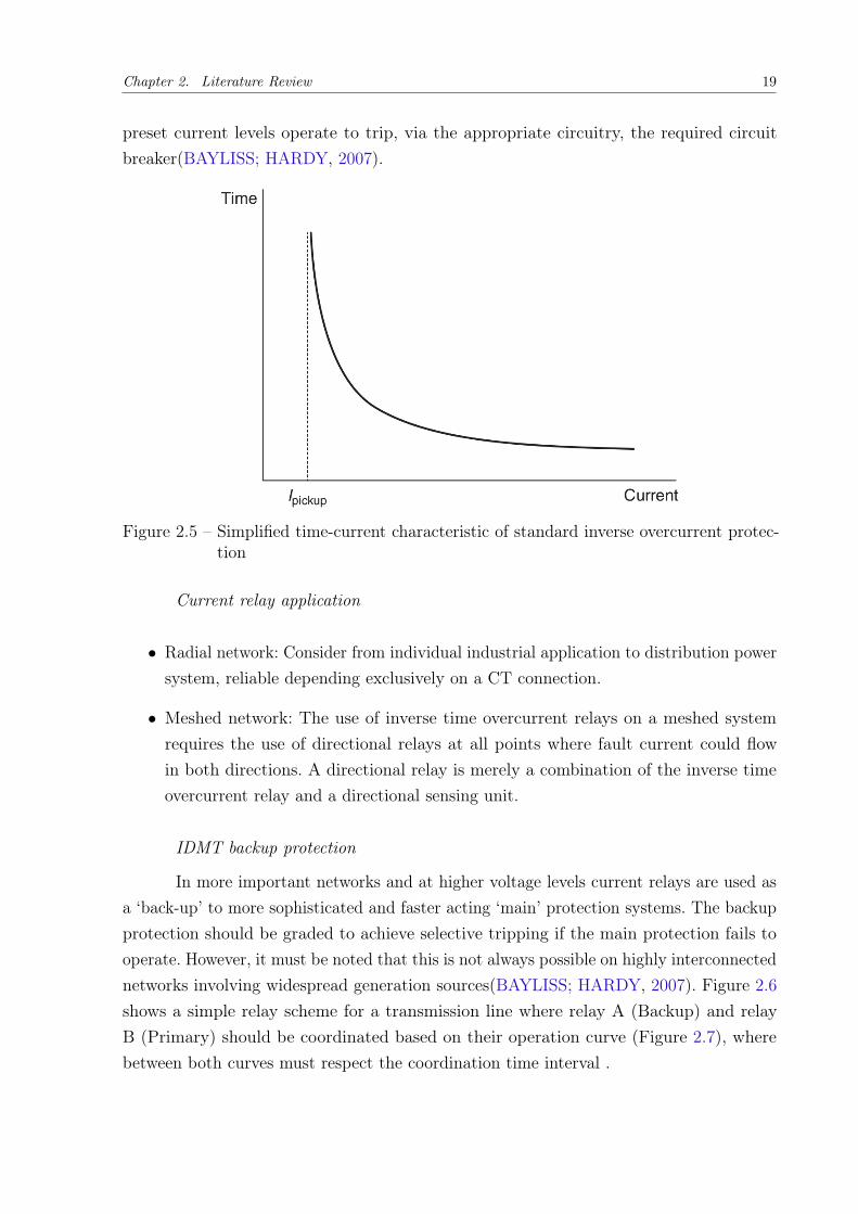
protection) . . . . . . . . . . . . . . . . . . . . . . . . . . . . . . . . . 17Figure 2.5 – Simplified time-current characteristic of standard inverse overcurrent
protection . . . . . . . . . . . . . . . . . . . . . . . . . . . . . . . . . . 19Figure 2.6 – Overcurrent protection for two serially connected feeders . . . . . . . . 20Figure 2.7 – Time-current characteristics with settings and fault currents for two
coordinated overcurrent relays . . . . . . . . . . . . . . . . . . . . . . . 20Figure 2.8 – Zones of protection of distance protection with indicative time delays
of operation for faults detected in each zone. . . . . . . . . . . . . . . . 21Figure 2.9 – Illustration of distance protection zone boundaries in the complex
impedance plane. . . . . . . . . . . . . . . . . . . . . . . . . . . . . . . 22Figure 3.1 – Critical fault locations for the coordination between overcurrent and
distance relays . . . . . . . . . . . . . . . . . . . . . . . . . . . . . . . 28Figure 3.2 – Feasible region for Primary-Backup Relay Considering TDS fixed. . . . 30Figure 3.3 – Feasible region for Primary-Backup Relay Considering PS fixed. . . . . 30Figure 3.4 – Overcurrent Relay 3D time plot considering TDS and PS Variation. . . 31Figure 4.1 – Ants build solutions, that is, paths from a source to a destination node. 32Figure 4.2 – Ants paths from the nest to the food. . . . . . . . . . . . . . . . . . . . 33Figure 4.3 – Structure of the solution archive used by ACOMV (SOLNON, 2007) In
this case, reduced to two variable types. . . . . . . . . . . . . . . . . . 35Figure 4.4 – Gaussian Kernel of the SA . . . . . . . . . . . . . . . . . . . . . . . . . 36Figure 4.5 – Flowchart for ACOMV . . . . . . . . . . . . . . . . . . . . . . . . . . . 38Figure 4.6 – F-RACE representation step by step until reach survivor. . . . . . . . . 43Figure 4.7 – Flowchart including high-quality initial solution built . . . . . . . . . . 44Figure 4.8 – Flowchart for Hybrid Scheme ACO-LP . . . . . . . . . . . . . . . . . . 46Figure 5.1 – Single-line diagram of the three-bus system. . . . . . . . . . . . . . . . 47Figure 5.2 – Single-line diagram of the six-bus system. . . . . . . . . . . . . . . . . 49Figure 5.3 – Single-line diagram of the eight-bus system. . . . . . . . . . . . . . . . 50Figure 5.4 – Single-line diagram of the nine-bus system. . . . . . . . . . . . . . . . . 52Figure 5.5 – Single-line diagram of the fifteen-bus system. . . . . . . . . . . . . . . . 54Figure 6.1 – OF Value for Single ACO, ACO NOT OPT, and ACO + IHQS for a
3-Bus System. . . . . . . . . . . . . . . . . . . . . . . . . . . . . . . . . 63Figure 6.2 – OF value Coordination with ACO-LP for a 3-Bus System . . . . . . . . 64
x
Figure 6.3 – Distance-DOCR Coordination with ACO-LP for a 3-Bus System . . . . 64Figure 6.4 – OF Value for Single ACO, ACO NOT OPT, and ACO + IHQS for a
6-Bus System. . . . . . . . . . . . . . . . . . . . . . . . . . . . . . . . . 68Figure 6.5 – OF value DOCR Coordination with ACO-LP for a 6-Bus System . . . 69Figure 6.6 – OF value Distance-DOCR Coordination with ACO-LP for a 6-Bus System 69Figure 6.7 – OF Value for Single ACO, ACO NOT OPT, and ACO + IHQS for a
8-Bus System. . . . . . . . . . . . . . . . . . . . . . . . . . . . . . . . . 75Figure 6.8 – Unfitness Value for Single ACO, ACO NOT OPT, and ACO + IHQS
for a 8-Bus System. . . . . . . . . . . . . . . . . . . . . . . . . . . . . . 76Figure 6.9 – OF Value for DOCR Coordination with ACO-LP for a 8-Bus System. . 76Figure 6.10–OF Value for Distance-DOCR Coordination with ACO-LP for a 8-Bus
System. . . . . . . . . . . . . . . . . . . . . . . . . . . . . . . . . . . . 77Figure 6.11–OF Value for Single ACO, ACO NOT OPT, and ACO + IHQS for a
9-Bus System. . . . . . . . . . . . . . . . . . . . . . . . . . . . . . . . . 80Figure 6.12–OF Value of DOCR Coordination with ACO-LP for a 9-Bus System. . 81Figure 6.13–Unfitness Value of DOCR Coordination with ACO-LP for a 9-Bus System. 81Figure 6.14–OF Value for Single ACO, ACO NOT OPT, and ACO + IHQS for a
15-Bus System. . . . . . . . . . . . . . . . . . . . . . . . . . . . . . . . 85Figure 6.15–OF Value for DOCR Coordination with ACO-LP for a 15-Bus System. 85

List of Tables
Table 3.1 – Overcurrent Relay Types . . . . . . . . . . . . . . . . . . . . . . . . . . 23Table 3.2 – IEEE Inverse Time Curve Constants . . . . . . . . . . . . . . . . . . . . 24Table 3.3 – IEC (BS) Inverse Time Curve Constants . . . . . . . . . . . . . . . . . . 24Table 3.4 – GE TYPE IAC Inverse Time Curve Constants . . . . . . . . . . . . . . 25Table 3.5 – Distance relays second zone configuration time interval . . . . . . . . . . 29Table 4.1 – The range of ACO parameters considered. . . . . . . . . . . . . . . . . . 44Table 5.1 – Short-circuit current values for normal and transient configuration for
a three-phase fault at the midpoint of the line, including CTR value /Three Bus Network . . . . . . . . . . . . . . . . . . . . . . . . . . . . . 48
Table 5.2 – Short-circuit current values for a fault at the near-end and far-end of theline / Three Bus Network . . . . . . . . . . . . . . . . . . . . . . . . . . 48
Table 5.3 – Short-circuit current values for a fault at the near-end and far-end of theline . . . . . . . . . . . . . . . . . . . . . . . . . . . . . . . . . . . . . . 49
Table 5.4 – Short-circuit current values for normal and transient configuration for afault at the midpoint of the line, including CTR value . . . . . . . . . . 51
Table 5.5 – Short-circuit current values for normal and transient configuration for afault at the midpoint of the line . . . . . . . . . . . . . . . . . . . . . . 53
Table 5.6 – Short-circuit current values for normal and transient configuration for afault at the midpoint of the line . . . . . . . . . . . . . . . . . . . . . . 55
Table 6.1 – Hundred Evaluation of DOCR Objective Function Value for 3-Bus System 57Table 6.2 – Hundred Evaluation of DOCR Algorithm Execution Time for 3-Bus System 57Table 6.3 – Tripping times for coordinated configuration - Mid-Point Fault for 3-bus
System . . . . . . . . . . . . . . . . . . . . . . . . . . . . . . . . . . . . 57Table 6.4 – Best solution found for 3-Bus System Mid-Point Fault of DOCR . . . . 58Table 6.5 – Top 10 feasible and optimal solutions from exhaustive LP solver for
three-bus system. . . . . . . . . . . . . . . . . . . . . . . . . . . . . . . 58Table 6.6 – Worst 5 feasible solutions from exhaustive LP solver for three-bus system. 58Table 6.7 – Hundred Evaluation of DOCR (Near-end and Far-end Fault) Objective
Function Value for 3-Bus System . . . . . . . . . . . . . . . . . . . . . . 58Table 6.8 – Hundred Evaluation of DOCR (Near-end and Far-end Fault) Algorithm
Execution Time for 3-Bus System . . . . . . . . . . . . . . . . . . . . . 59Table 6.9 – Tripping times for coordinated configuration - Near-end and Far-end
Fault for 3-bus System . . . . . . . . . . . . . . . . . . . . . . . . . . . 59Table 6.10–Tripping times for coordinated (Hybrid) configuration - Near-end and
Far-end Fault for 3-bus System . . . . . . . . . . . . . . . . . . . . . . 60
xii
Table 6.11–Best solution found for 3-Bus System (Near-end and Far-end Fault) ofDOCR . . . . . . . . . . . . . . . . . . . . . . . . . . . . . . . . . . . . 60
Table 6.12–Hundred Evaluation of Distance-DOCR Objective Function Value for3-Bus System . . . . . . . . . . . . . . . . . . . . . . . . . . . . . . . . . 60
Table 6.13–Hundred Evaluation of Distance-DOCR Algorithm Execution Time for3-Bus System . . . . . . . . . . . . . . . . . . . . . . . . . . . . . . . . . 61
Table 6.14–Tripping times for coordinated configuration - Distance / DOCR for3-bus System . . . . . . . . . . . . . . . . . . . . . . . . . . . . . . . . . 61
Table 6.15–Tripping times for coordinated (Hybrid) configuration - Distance / DOCRfor 3-bus System . . . . . . . . . . . . . . . . . . . . . . . . . . . . . . . 61
Table 6.16–Best solution found for 3-Bus System (Near-end and Far-end Fault) ofDistance-DOCR . . . . . . . . . . . . . . . . . . . . . . . . . . . . . . . 62
Table 6.17–Survivors of the F-RACE Algorithm for 3-Bus System . . . . . . . . . . 62Table 6.18–Comparing for Survivors of the F-RACE Algorithm for 3-Bus System . 63Table 6.19–Results Comparison for 3-Bus System Mid-Point Fault DOCR . . . . . 65Table 6.20–Results Comparison for 3-Bus System (Near-end and Far-end Fault) DOCR 65Table 6.21–Hundred Evaluation of DOCR (Near-end and Far-end Fault) Value for
6-Bus System . . . . . . . . . . . . . . . . . . . . . . . . . . . . . . . . . 66Table 6.22–Hundred Evaluation of DOCR Algorithm Execution Time for 6-Bus System 66Table 6.23–Best solution found for 6-Bus System (Near-end and Far-end Fault) of
DOCR . . . . . . . . . . . . . . . . . . . . . . . . . . . . . . . . . . . . 66Table 6.24–Hundred Evaluation of Distance-DOCR Coordination of Value for 6-Bus
System . . . . . . . . . . . . . . . . . . . . . . . . . . . . . . . . . . . . 67Table 6.25–Hundred Evaluation of Distance-DOCR Coordination Algorithm Execu-
tion Time for 6-Bus System . . . . . . . . . . . . . . . . . . . . . . . . . 67Table 6.26–Best solution found for 6-Bus System (Near-end and Far-end Fault) of
Distance-DOCR . . . . . . . . . . . . . . . . . . . . . . . . . . . . . . . 67Table 6.27–Survivors of the F-RACE Algorithm for 6-Bus System . . . . . . . . . . 67Table 6.28–Comparing for Survivors of the F-RACE Algorithm for 6-Bus System . 68Table 6.29–Results Comparison for 6-Bus System Mid-Point Fault DOCR . . . . . 70Table 6.30–Hundred Evaluation of DOCR Objective Function Value for 8-Bus System 70Table 6.31–Hundred Evaluation of DOCR Algorithm Execution Time for 8-Bus System 71Table 6.32–Best solution found for 8-Bus System (Near-end Fault) of DOCR . . . . 71Table 6.33–Top 10 feasible & optimal solutions from exhaustive from limited LP
solver for eight-bus system. . . . . . . . . . . . . . . . . . . . . . . . . . 72Table 6.34–Hundred Evaluation of Distance-DOCR Objective Function Value for
8-Bus System . . . . . . . . . . . . . . . . . . . . . . . . . . . . . . . . . 72Table 6.35–Hundred Evaluation of Distance-DOCR Algorithm Execution Time for
8-Bus System . . . . . . . . . . . . . . . . . . . . . . . . . . . . . . . . . 73

xiii
Table 6.36–Best solution found for 8-Bus System (Near-end) of Distance-DOCR . . 73Table 6.37–Survivors of the F-RACE Algorithm for 8-Bus System . . . . . . . . . . 74Table 6.38–Comparing for Survivors of the F-RACE Algorithm for 8-Bus System . 74Table 6.39–Results Comparison for 8-Bus System Fault DOCR . . . . . . . . . . . . 77Table 6.40–Hundred Evaluation of DOCR Objective Function Value for 9-Bus System 78Table 6.41–Hundred Evaluation of DOCR Algorithm Execution Time for 9-Bus System 78Table 6.42–Best TDS solution found for 9-Bus System (Near-end and Far-end Fault)
of DOCR . . . . . . . . . . . . . . . . . . . . . . . . . . . . . . . . . . . 78Table 6.43–Best PS solution found for 9-Bus System (Near-end and Far-end Fault)
of DOCR . . . . . . . . . . . . . . . . . . . . . . . . . . . . . . . . . . . 79Table 6.44–Survivors of the F-RACE Algorithm for 9-Bus System . . . . . . . . . . 79Table 6.45–Comparing for Survivors of the F-RACE Algorithm for 9-Bus System . 80Table 6.46–Results Comparison for 9-Bus System Fault DOCR . . . . . . . . . . . . 82Table 6.47–Hundred Evaluation of DOCR Objective Function Value for 15-Bus System 82Table 6.48–Hundred Evaluation of DOCR Algorithm Execution Time for 15-Bus
System . . . . . . . . . . . . . . . . . . . . . . . . . . . . . . . . . . . . 82Table 6.49–Best TDS solution found for 15-Bus System (Near-end and Far-end Fault)
of DOCR . . . . . . . . . . . . . . . . . . . . . . . . . . . . . . . . . . . 83Table 6.50–Best PS solution found for 15-Bus System (Near-end and Far-end Fault)
of DOCR . . . . . . . . . . . . . . . . . . . . . . . . . . . . . . . . . . . 83Table 6.51–Survivors of the F-RACE Algorithm for 15-Bus System . . . . . . . . . 84Table 6.52–Comparing for Survivors of the F-RACE Algorithm for 15-Bus System . 84Table 6.53–Results Comparison for 15-Bus System Mid-Point Fault DOCR . . . . . 86Table 6.54–Parameter influence for all tested system . . . . . . . . . . . . . . . . . 86Table A.1–Tripping times for coordinated configuration - 6 Bus System . . . . . . . 104Table A.2–Tripping times for coordinated (Hybrid) configuration - 6 Bus System . 105Table A.3–Tripping times for coordinated configuration - Distance / DOCR for
6-bus System - Part I . . . . . . . . . . . . . . . . . . . . . . . . . . . . 106Table A.4–Tripping times for coordinated configuration - Distance / DOCR for
6-bus System - Part II . . . . . . . . . . . . . . . . . . . . . . . . . . . . 106Table A.5–Tripping times for coordinated configuration (Hybrid) - Distance / DOCR
for 6-bus System - Part I . . . . . . . . . . . . . . . . . . . . . . . . . . 107Table A.6–Tripping times for coordinated configuration (Hybrid) - Distance / DOCR
for 6-bus System - Part II . . . . . . . . . . . . . . . . . . . . . . . . . . 108Table A.7–Tripping times for coordinated configuration - 8 Bus System . . . . . . . 108Table A.8–Tripping times for coordinated (Hybrid) configuration - 8 Bus System . 109Table A.9–Tripping times for coordinated configuration - Distance / DOCR for
8-bus System . . . . . . . . . . . . . . . . . . . . . . . . . . . . . . . . . 109

xiv
Table A.10–Tripping times for coordinated (Hybrid) configuration - Distance / DOCRfor 8-bus System . . . . . . . . . . . . . . . . . . . . . . . . . . . . . . . 110
Table A.11–Tripping times for coordinated configuration - 9 Bus System . . . . . . . 111Table A.12–Tripping times for coordinated (Hybrid) configuration - 9 Bus System . 112Table A.13–Tripping times for coordinated configuration - 15 Bus System . . . . . . 113Table A.14–Tripping times for coordinated (Hybrid) configuration - 15 Bus System . 114

List of Abbreviations and Acronyms
ABNT Associação Brasileira de Normas Técnicas
ACO ant colony optimization
ACOR ant colony optimization for continuous domain
BBO Biogeography Based Optimization
BR backup relay
CO combinatorial optimization
COPEL Companhia Paranaense de Energia
CSA Cuckoo Search Algorithm
CT current transformer
CTI coordination time interval
CTR current transformer rate
CV constraints violations
CVT capacitor voltage transformer
DG distributed generation
DOCR directional overcurrent relays
DT definite time
DZ-1 Zone 1 for a distance relay
GA genetic algorithm
GACB Genetic Algorithm Chu-Beasley
GE General Electric
HSOC high set overcurrent
I/F-Race Iterated F-Race Algorithm
IAC family of overcurrent relays from General Electric (GE)
IDMT inverse definite minimum time

xvi
IEC International Electrotechnical Commission
IEEE Institute of Electrical and Electronics Engineers
IHQS initial high-quality solution
ISO International Organization for Standardization
LP linear programming
MDE Modified Differential Evolution
MDE5 Modified Differential Evolution v5
MINLP mixed-integer nonlinear programming
MVOP mixed-variable optimization problem
NBA No Backup Available
NFE number of function evaluation
NLP nonlinear programming
OCDE Opposition Based Chaotic Differential Evolution
OF objective function
OSL OSL Solver
PR primary relay
PS plug setting
PSO Particle Swarm Optimization
RST Rhetorical Structure Theory
SA solution archive
SBB Standard Branch-and-Bound
SEF Sensitive earth fault
SLS stochastic local search
SOA Seeker Optimization Algorithm
SQP Sequential Quadratic Programming
TDS time dial setting

xvii
TSS Total Search Space
VSS Valid Search Space
VT voltage transformer

List of Symbols
Relays and Coordination
A, p, B Constant parameters for IEEE Relays.
K, E Constant parameters for IEC Relays.
A to E Constant parameters for IAC Relays.
I Input current.
Ipickup Pickup Current.
∆t Coordination Time Interval, also CTI.
tik Operating time of the relay i for a fault in k.
CTRi Current Transformer Ratio for relay i.
n Number of relays to coordinate.
TDSmini Minimum value of TDS of relay Ri.
TDSmaxi Maximum value of TDS of relay Ri.
PSmini Minimum value of PS of relay Ri.
PSmaxi Maximum value of PS of relay Ri.
tOCik Operating time of the primary DOCR i for a fault k.
tZ2i Time defined for the second zone of each distance relay.
tZ2i min Minimum value of tZ2
i of relay Ri.
tZ2i max Maximum value of tZ2
i of relay Ri.
Model for Mixed-variable Optimization Problems
R A model for Mixed-variable Optimization Problems
S Search space S
Ω Set of constraints among the variables.
o Ordinal variables.
c Categorical variables.
xix
d Discrete variables.
r Continuous variables.
ACO for Mixed-variable Optimization Problems
k Size of solutions in the SA.
Sj Individuals Solutions from SA
ns Number of new solutions (ants).
ωj Weight for a solution j in the SA.
q Parameter of the algorithm (qr Continuous qc Categorical)
h1 h2 Weighting factors for increasing or decreasing the influence of fitnessand unfitness function, respectively.
ε Tolerance for stop criteria.
ξ Parameter related to pheromone persistence or convergence.
uil Number of solutions that use PSi for the categorical variable i in theSA.
η Number of values from PS vector available ones that are not used bythe SA.
σQF Stagnation of the QF.
F-RACE
Θ Possibly infinite set of candidate configurations.
I Possibly infinite set of instances.
pI Probability measure over the set I.
t Computation time.
c Cost measure of a configuration.
pC Probability measure over the set C.
T Total amount of time available for experimenting with the given can-didate configurations on the available instances before delivering theselected configuration.
L Number of iterations.

xx
l Number of actual iteration.
d Number of parameters.
Bl Computational budget in iteration l.
Bused Total computational budget used until iteration l − 1.
Nmin Number of candidate configurations remain.
Nsurvive Number of candidates that withstand the race.
rz Rank of of the configuration z.
Contents
List of Figures . . . . . . . . . . . . . . . . . . . . . . . . . . . . . ix
List of Tables . . . . . . . . . . . . . . . . . . . . . . . . . . . . . xi
List of Abbreviations and Acronyms . . . . . . . . . . . . . . . xv
List of Symbols . . . . . . . . . . . . . . . . . . . . . . . . . . . . xviii
1 INTRODUCTION . . . . . . . . . . . . . . . . . . . . . . . . . . 11.1 General considerations . . . . . . . . . . . . . . . . . . . . . . . . . . 11.2 Statement of the problem . . . . . . . . . . . . . . . . . . . . . . . 31.3 Objectives . . . . . . . . . . . . . . . . . . . . . . . . . . . . . . . . 41.4 Methodology . . . . . . . . . . . . . . . . . . . . . . . . . . . . . . . 41.5 Outline of the dissertation . . . . . . . . . . . . . . . . . . . . . . 6
2 LITERATURE REVIEW . . . . . . . . . . . . . . . . . . . . . . 72.1 State of the Art . . . . . . . . . . . . . . . . . . . . . . . . . . . . . 72.2 Protective Relaying . . . . . . . . . . . . . . . . . . . . . . . . . . . 112.2.1 Power System Protection Components . . . . . . . . . . . . . . 122.2.2 Instrument Transformers . . . . . . . . . . . . . . . . . . . . . . . 122.2.3 Zones of Protection . . . . . . . . . . . . . . . . . . . . . . . . . . . 142.2.4 Protection system philosophies . . . . . . . . . . . . . . . . . . . 152.2.5 Primary and backup protection . . . . . . . . . . . . . . . . . . . 172.2.6 Protection techniques . . . . . . . . . . . . . . . . . . . . . . . . . 182.2.7 Modernization of the Protection System . . . . . . . . . . . . . 22
3 MATHEMATICAL FORMULATION . . . . . . . . . . . . . . 233.1 Mathematical Modeling DOCR . . . . . . . . . . . . . . . . . . . 233.1.1 IEEE Curves . . . . . . . . . . . . . . . . . . . . . . . . . . . . . . . 243.1.2 IEC Curves . . . . . . . . . . . . . . . . . . . . . . . . . . . . . . . . 243.1.3 IAC Curves . . . . . . . . . . . . . . . . . . . . . . . . . . . . . . . 253.1.4 I2t Curves . . . . . . . . . . . . . . . . . . . . . . . . . . . . . . . . 253.1.5 Objective Function . . . . . . . . . . . . . . . . . . . . . . . . . . . 253.1.6 Coordination Constraints . . . . . . . . . . . . . . . . . . . . . . . 263.2 Mathematical Modeling DOCR & Distance . . . . . . . . . . . 273.2.1 Objective Function . . . . . . . . . . . . . . . . . . . . . . . . . . . 283.2.2 Coordination Constraints . . . . . . . . . . . . . . . . . . . . . . . 28
xxii
3.3 Feasible Region and Problem Characterization . . . . . . . . . 30
4 IMPLEMENTATION . . . . . . . . . . . . . . . . . . . . . . . . 324.1 Ant Colony Optimization . . . . . . . . . . . . . . . . . . . . . . . 324.2 Model for Mixed-variable Optimization Problems . . . . . . . 334.3 ACO for Mixed-variable Optimization Problems . . . . . . . . 344.3.1 Codification . . . . . . . . . . . . . . . . . . . . . . . . . . . . . . . 344.4 Construction of a solution (an ant) . . . . . . . . . . . . . . . . . 354.4.1 ACOMV Parameters . . . . . . . . . . . . . . . . . . . . . . . . . . . 364.5 Restart Mechanism . . . . . . . . . . . . . . . . . . . . . . . . . . . 374.6 Algorithm and Flowchart . . . . . . . . . . . . . . . . . . . . . . . 374.7 Analysis of ACO parameters . . . . . . . . . . . . . . . . . . . . . 374.7.1 F-RACE approach . . . . . . . . . . . . . . . . . . . . . . . . . . . 384.7.2 Algorithm Configuration Problem . . . . . . . . . . . . . . . . . 404.7.3 Iterated F-Race Algorithm . . . . . . . . . . . . . . . . . . . . . . . 414.8 High-Quality Initial Solution . . . . . . . . . . . . . . . . . . . . . 444.9 Hybrid Technique ACO-LP . . . . . . . . . . . . . . . . . . . . . . 454.10 Solution Space Estimate - Linear Relaxation . . . . . . . . . . . 45
5 TESTING SYSTEMS . . . . . . . . . . . . . . . . . . . . . . . . 475.1 System I: Three Bus Network . . . . . . . . . . . . . . . . . . . . 475.2 System II: Six Bus Network . . . . . . . . . . . . . . . . . . . . . 485.3 System III: Eight Bus Network . . . . . . . . . . . . . . . . . . . 505.4 System IV: Nine Bus Network . . . . . . . . . . . . . . . . . . . . . 515.5 System V: Fifteen Bus Network . . . . . . . . . . . . . . . . . . . 53
6 RESULTS AND DISCUSSIONS . . . . . . . . . . . . . . . . . . 566.1 System I: Three Bus Network . . . . . . . . . . . . . . . . . . . . 566.1.1 DOCRs Only . . . . . . . . . . . . . . . . . . . . . . . . . . . . . . . 566.1.2 Distance and DOCRs (Near-end and Far-end Fault) . . . . . . 606.1.3 ACO Parameters Optimization with F-RACE . . . . . . . . . . 626.1.4 Validation . . . . . . . . . . . . . . . . . . . . . . . . . . . . . . . . . 636.2 System II: Six Bus Network . . . . . . . . . . . . . . . . . . . . . 656.2.1 DOCRs Only . . . . . . . . . . . . . . . . . . . . . . . . . . . . . . . 656.2.2 Distance and DOCRs . . . . . . . . . . . . . . . . . . . . . . . . . 666.2.3 ACO Parameters Optimization with F-RACE . . . . . . . . . . 676.2.4 Validation . . . . . . . . . . . . . . . . . . . . . . . . . . . . . . . . . 686.3 System III: Eight Bus Network . . . . . . . . . . . . . . . . . . . 706.3.1 DOCRs Only . . . . . . . . . . . . . . . . . . . . . . . . . . . . . . . 706.3.2 Distance and DOCRs . . . . . . . . . . . . . . . . . . . . . . . . . 72

xxiii
6.3.3 ACO Parameters Optimization with F-RACE . . . . . . . . . . 736.3.4 Validation . . . . . . . . . . . . . . . . . . . . . . . . . . . . . . . . . 746.4 System IV: Nine Bus Network . . . . . . . . . . . . . . . . . . . . 776.4.1 DOCRs Only . . . . . . . . . . . . . . . . . . . . . . . . . . . . . . . 786.4.2 ACO Parameters Optimization with F-RACE . . . . . . . . . . 796.4.3 Validation . . . . . . . . . . . . . . . . . . . . . . . . . . . . . . . . . 806.5 System V: Fifteen Bus Network . . . . . . . . . . . . . . . . . . . 826.5.1 DOCRs Only . . . . . . . . . . . . . . . . . . . . . . . . . . . . . . . 826.5.2 ACO Parameters Optimization with F-RACE . . . . . . . . . . 836.5.3 Validation . . . . . . . . . . . . . . . . . . . . . . . . . . . . . . . . . 846.6 Discussions and Final Considerations . . . . . . . . . . . . . . . 86
7 CONCLUSION . . . . . . . . . . . . . . . . . . . . . . . . . . . . 88
8 RECOMMENDATIONS FOR FUTURE WORK . . . . . . . . 89
BIBLIOGRAPHY . . . . . . . . . . . . . . . . . . . . . . . . . . 90
APPENDIX 103
APPENDIX A – COORDINATION TIMES RESULTS . . . 104A.1 System II: Six Bus Network . . . . . . . . . . . . . . . . . . . . . 104A.1.1 DOCRs Only . . . . . . . . . . . . . . . . . . . . . . . . . . . . . . . 104A.1.2 Distance and DOCRs . . . . . . . . . . . . . . . . . . . . . . . . . 105A.2 System III: Eight Bus Network . . . . . . . . . . . . . . . . . . . 108A.2.1 DOCRs Only . . . . . . . . . . . . . . . . . . . . . . . . . . . . . . . 108A.2.2 Distance and DOCRs . . . . . . . . . . . . . . . . . . . . . . . . . 109A.3 System IV: Nine Bus Network . . . . . . . . . . . . . . . . . . . . 110A.3.1 DOCRs Only . . . . . . . . . . . . . . . . . . . . . . . . . . . . . . . 110A.4 System V: Fifteen Bus Network . . . . . . . . . . . . . . . . . . . 113A.4.1 DOCRs Only . . . . . . . . . . . . . . . . . . . . . . . . . . . . . . . 113
1
1 Introduction
1.1 General considerations
In an electric power system design, system protection is an important consideration.Without system protection, the power system itself, which is intended to be of benefit tothe facility in question, would itself become a hazard.
Power systems are designed to be as fault-free as possible through careful design,proper equipment installation, and periodic equipment maintenance. However, even whenthese practices are followed, it is not practical to design a power system to completelyeliminate faults from occurring (STENANE, 2014).
System faults usually, but not always, provide significant changes in the systemquantities, which can be used to distinguish between tolerable and intolerable systemconditions. These changing quantities include overcurrent, over or under-voltage, power,power factor or phase angle, power or current direction, impedance, frequency, temperature,physical movements, pressure, and contamination of the insulating quantities. The mostcommon fault indicator is a sudden and generally significant increase in the current;consequently, overcurrent protection is widely used (BLACKBURN; DOMIN, 2006).
A detailed model of a protection system is complex and will usually consist ofthree major parts: instrument transformers, protective relays, and circuit breakers. Theinstrument transformers lower the power system voltages to safe working levels. Theprotective relays receive information about the operating conditions of the high-voltagepower system via the instrument transformers (MARTINEZ-VELASCO, 2015). TheInstitute of Electrical and Electronics Engineers (IEEE) defines a protective relay asa relay whose function is to detect defective lines or apparatus or other power systemconditions of an abnormal or dangerous nature and to initiate appropriate control circuitaction (IEEE, 2000).
According to (BLACKBURN; DOMIN, 2006), there are five basic facets of protectiverelay application:
1. Reliability: assurance that the protection will perform correctly.
2. Selectivity: maximum continuity of service with minimum system disconnection.
3. Speed of operation: minimum fault duration and consequent equipment damage andsystem instability.

Chapter 1. Introduction 2
4. Simplicity: minimum protective equipment and associated system to achieve theprotection objectives.
5. Economics: maximum protection at minimal total cost.
If all five basic objectives could be achieved to their maximum requirement levelit would be the ideal scenario but not a real-life situation. Thus, the protection engineermust evaluate these as restrictions for maximizing the protection of the system.
The process of choosing settings or time delay characteristics of protective devices,such that operation of the devices will occur in a specified order to minimize customerservice interruption and power system isolation due to a power system disturbance isknown as coordination of protection (IEEE, 2000).
Overcurrent and Distance relays are mostly used for transmission and sub-transmissionprotection systems.
For overcurrent relays, the coordination is performed using linear or non-linearprogramming techniques but to avoid the complexity of the non-linear programmingmethods, coordination problem for overcurrent relays is commonly formulated as a linearprogramming (KALAGE; GHAWGHAWE, 2016). The optimization techniques usingmethods as Simplex, Two-phase Simplex, and Dual Simplex present a disadvantage becausethey are based on an initial basic solution and may be trapped in the local minimumvalues. Intelligent optimization techniques such as genetic algorithm (GA) can adjust thesetting of the relays without the mentioned difficulties but requiring a modification of theobjective function and constraints (NOGHABI et al., 2009), trending heuristics techniquesto solve the problem.
The distance protection is one of the most common protection types since it givesby measuring voltage and current at one point already a very selective information aboutthe fault. However, high time coherence between current and voltage in the order of 1µs
is needed for correct results (BRAND; De Mesmaeker, 2013). Distance relays can beused as main or backup protection, to protect the transmission line or power transformer.Nowadays, numerical distance relays have been used widely replacing the electromechanicaland static distance relays (IDRIS et al., 2013).
In the cases that the distance relay is considered to be the main relay and theovercurrent one is the backup relay, it is necessary to find the critical fault locations. Theseare critical fault locations at which the time margin (∆t) between main distance relayand backup overcurrent relay is at a minimum. The coordination is made based on theconstraints derived from the values (∆t) for critical fault locations (SINGH et al., 2012).The object function is developed by adding a new term that is the constraint related tothe coordination of the distance and overcurrent relays when a fault occurs at the critical

Chapter 1. Introduction 3
location.
1.2 Statement of the problem
The overcurrent protection has an extended implementation in the electrical powersystem compare to directional overcurrent and distance protection, a simpler operationalprinciple leads to low-cost applications. In situations where a distributed generator ispresent, a radial scheme is no longer valid because power flow eventually will change,accordingly, modern transmission, sub-transmission, and distribution protection systemhave many similarities. Since overcurrent protection protects from faults in one direction, itcannot be implemented in these circumstances. In such, a situation directional overcurrentor distance protection would be the ideal protection. Directional overcurrent detects afault in forward and reverse directions and distance protection uses zones to protect thefeeder.
The coordination problem is widely solved using a linear programming implementa-tion as explained in Urdaneta et al. (1988). Many different techniques have been proposedand applied since then. But in this case, the coordination problem requires reformulatingthe objective function to combine overcurrent and distance settings. For overcurrent relaysfinding the time dial setting is based on the mathematical statement of the sensitivity,speed, security and selectivity conditions associated with the traditional relay coordinationproblem. Perez and Urdaneta (2001) proposes a procedure to include backup definite-timerelays in the process of computing the time dial setting (TDS) of directional overcurrent re-lays (DOCR) with inverse time curves. This is useful in transmission and sub-transmissionsystems which have a mixed scheme with directional overcurrent and distance relays. Forthe particular case of the coordination of directional overcurrent relays of distance relays,it was proposed to change constraints with the results of improvement of selectivity.
In linear programming techniques, it is not possible to select overcurrent relayscharacteristic besides relays’ time dial setting (TDS) to have the optimal coordination. Insome cases of overcurrent/distance relays coordination, it is necessary to find the criticalfault locations. A mixed protection scheme with distance relays formulated in Abyanehet al. (2008) has been modified in such a way that five different critical points as thefault position are taken into account and Chabanloo et al. (2011) adding some new termsfulfill optimal combined coordination of distance and overcurrent relays, using GA-basedHeuristic.
Sadeh et al. (2011) proposed to perform optimal coordination between distance andovercurrent relays for every second zone of distance relays; finding time multiplies settingand second zone time for each relay by linear programming, and computing of pickupcurrent by using particle swarm optimization. This hybrid particle swarm optimization

Chapter 1. Introduction 4
was successful in achieving a better coordination than linear programming. According tothis reference obtained results of particle swarm optimization and genetic algorithm for asample network, are equal, but particle swarm optimization performs coordination faster.For combined optimization of relays coordination, Singh et al. (2012) stands differentialevolutionary algorithm gives no-miscoordination and coordination time margin is notviolated as seen in the result obtained from GA.
1.3 Objectives
The main objective is to present a study of different methodologies for the coordina-tion of distance and/or overcurrent relays in electric power systems, using a mathematicaloptimization technique and a computational tool to determine the best settings for therelays been selective.
In order to reach the main objective, the above specific objectives are defined:
• Review of specialized methodologies used in the optimal coordination of distanceand overcurrent relays, both as individual and/or combined configuration.
• Formulate the problem of relay coordination like a mathematical optimizationproblem.
• Establish a procedure for the transformation of non-linear mathematical models intolinear models applied to the relay study case.
• Develop a metaheuristic algorithm to solve the coordination problem.
• Implement a tool able to improve results, according to the comparison with precededinvestigations.
• Analyze a tuning process for the heuristic applied in order to increase the performanceof the algorithm and maximize the protection facets.
• Compare and evaluate the results applying the proposed methodology to the literaturereviewed.
1.4 Methodology
This dissertation is based on the analysis of results obtained through an appliedmathematical modeling procedure to solve a combine relays coordination theory. In thiscase of study distance and overcurrent relays as individual and as a combine protectionsystem are evaluated in order to obtain potential configuration schemes into coordinationproblem.

Chapter 1. Introduction 5
In order to achieve a successful implementation, qualitative research is required togain an understanding and generate a new approach to combine relay coordination forlater quantitative research, based on measuring of the testing systems fault response.
Qualitative research involves investigating the subjects relate to power systemprotection and the mathematical techniques applied to relays coordination, with anemphasis on the formulation of an objective function and his constraints. In the literature,different methods are applied to solve the coordination problem but this work focuseson an ant colony optimization (ACO) presenting a significant contribution to this study.Computational modeling to run tests on actual power systems, changing the topology tocompare evaluation results with literature review as quantitative research.
The bibliographic review was performed constantly throughout the work, main-taining the trends in the research of protection systems, besides its importance of otheractivities.
In essence, the step of mathematical modeling deals with an extension of what is onthe literature review, being dedicated to the analysis, characterization, reproduction, andcomparison of existing models and how they may be improved. At this point, it is possibleto learn and implement different solutions to problems related to relay coordination, linkedto the latest advances, which allow the characterization and comparison of such solutionswith new solution techniques. In this way, it offers an in-depth understanding of thesolutions of problems present in the literature, highlighting its advantages, deficienciesand specific details of the procedure, opening the way for possible improvements.
It is also worth mentioning that the comparing of results is done through simulationsmade from routines built for/on Matlab, which constitutes a high-level language, facilitatingand accelerating this stage because it offers practicality in the construction of functionsand routines. In addition, in the comparative phase, different solutions of problems of thesame kind are analyzed and compared in a fair way among each other, being evaluatedtheir performance and complexity.
The main contribution of this work is made through the augmentations to themathematical model introducing distance relay seeking for coordination improvementconsidering an extra-level protection with existing devices, whether own protection zoneor corresponding backup zones. Another major contribution in the optimization area isthe algorithm parameters optimization describing a specific technique to find optimalparameters to get better output from the implemented algorithm. Also relevant would beexhaustive search process to validate metaheuristic results.
Results obtained, overcome some precedents values validating the new algorithmas novel coordination problem solution, besides introducing a new base to combinedistance and overcurrent relay coordination, with a feasible model to future works and/or

Chapter 1. Introduction 6
implementation.
1.5 Outline of the dissertation
The dissertation is organized as follows:
Chapter 1: Introduction.
This chapter provides the purpose, statement of the problem, objectives, andresearch methodology of the project.
Chapter 2: Literature Review.
This chapter gives a State-of-the-Art resume and summarizes protective relayingand the basics schemes required to understand relays as a protective device and theimportance of their coordination.
Chapter 3: Mathematical Formulation.
In Chapter 3, the development of a mathematical formulation for distance andovercurrent coordination with limitation for each topology and actual consideration forthis problem.
Chapter 4: Implementation.
This chapter presents an overview of methodologies applied to relay coordination,with an implementation of Ant Colony Optimization technique, for multi-variable problems,developing a tool for the analysis of ACO parameters and optimizing them, besides aHybrid technique based on ACO and Linear Programming.
Chapter 5: Testing Systems.
System types, configuration, and data to apply proposed methodology to generateresults to compare.
Chapter 6: Results and Discussions.
In this chapter, the results, and discussions of the applied methodologies. Presentingtables and figures to corroborate results obtained.
Chapter 7: Conclusions.
The conclusions based on research discussions.
Chapter 8: Recommendations for Future Work
Future research trend line to continuing this work.

7
2 Literature Review
2.1 State of the Art
The incremental quantity of protection technologies impact in faults cleared faster,improving safety with a better power system stability, and preserved equipment lifeas consequence. Above smart grids design, network topologies are changing-intensively,changes must be deemed for the protection devices in order to heighten their performance.Classical coordination model is still valid but only for single instances of the daily networkload profile. Trending brings fast solving techniques able to process dynamic data keepingsystem all-time coordinated (SHIH; ENRIQUEZ, 2014; SHIH et al., 2017; ENRÍQUEZ;MARTÍNEZ, 2007; PIESCIOROVSKY; SCHULZ, 2017).
Optimal coordination of DOCRs in interconnected power systems originally byUrdaneta et al. (1988) presented two types of tap settings namely plug setting (PS) andTDS to be calculated. Mixed Protection Scheme, composed of distance relays and DOCRsrequires considering both relays because separate relay computation would lead to loss ofselectivity. Perez and Urdaneta (2001) model considers the best setting for the second zonethat assures selectivity differs from used in distance schemes, mixed configurations normallyare misestimated due to complex topologies and system-inside considerations to formulatean exact model, this mixed scheme brought back by Chabanloo et al. (2011), Singh et al.(2012) in-light the advantage over low speed of overcurrent relay forcing the applicationof distance relay for protection transmission system, even when miscoordination existfor sub-transmission systems usually work under those approaches; Ahmadi et al. (2017)studies pickup current effect on reduction of discrimination times improving coordination.
A concept of robust coordination conferred by Costa et al. (2017), which analyzes aclassical coordination model but counting different scenarios where the data of the systemis continuously changing and the selectivity is no longer correct. Recently, Yazdaninejadiet al. (2017) shows a different kind of coordination for meshed distribution networks,previously developed by Zeineldin et al. (2015), where dual setting relays are provided withtwo inverse time-current characteristics whose parameters will rely on the fault direction,adding an extra level of protection.
In adaptive protection schemes, it is necessary to compute the DOCRs parametersat each topological change (SHIH et al., 2014; CHEN; LEE, 2014; CORRÊA et al., 2015;SHIH et al., 2015). A practical implementation of adaptive protection is also reported inPiesciorovsky and Schulz (2017). Modern power systems with the addition of distributedgeneration (DG) impact on protective relaying (GEORGE et al., 2013), especially in

Chapter 2. Literature Review 8
radial systems where coordination is performed with no-directional units (HUSSAIN et al.,2013; CHEN et al., 2013), accordingly request the implementation of a meshed networkformulation (YANG et al., 2013; SRIVASTAVA et al., 2016)
An introduction to heuristic techniques came to treat the non-linear variable PS,the new evolutionary algorithm applied in Mansour et al. (2007), Zeineldin et al. (2005)shows and advantage for implementation, derivate from simplicity and robustness ofGA principle. Also, hybrid methods rise for the benefit of reducing the major probleminto small search spaces LP compatible (SINGH et al., 2011). A specialized GeneticAlgorithm Chu-Beasley (GACB) that uses an efficient local search, finding solutions tothe coordination problem with very low computation times is presented in Kida (2016),this guarantees an applicability in smart grid systems.
The ant colony optimization (ACO) was introduced by Dorigo et al. (1996) a novelnature-inspired metaheuristic for the solution combinatorial optimization (CO) problems.The ACO is inspired by the foraging behavior of real ants. Ants food search beginsexploring the area surrounding their nest in a random manner. When an ant finds a foodsource, proceeds to evaluate quantity and quality taking some back to the nest. During thisprocess, ants deposit a tale of pheromones that create trails for others to follow; increasingthe probability of finding food sources.
ACO common implementation is extended to multiple CO problems. But for high-resolution problem CO approach is not convenient, Socha and Dorigo (2008) introducedan ACO expansion to continuous domains named ACOR this algorithm close to originalformulation affords a convenience with the possibility of tackling mixed discrete-continuousvariables as develops Solnon (2007) later. The advantage of this algorithm compared toGA is the role of global memory played by the pheromone matrix, which leads to betterand faster solution convergence (SHIH et al., 2015).
Initial solutions for ACO is commonly generated using a normal random processwithin feasible space for each variable (BLUM, 2005). Machine learning algorithms measureperformance based on function evaluations, but for big sizes problem with a high number ofpossible combinations, computational time could be compromised. Evolutionary algorithmslook for start evaluation closer to the global optimal and enhancing convergence and solutionquality (ZHANG et al., 2011).
The performance of heuristic algorithms is known to be sensitive to the valuesassigned to its parameters. Ordinarily, studies provide reasonable ranges in which toinitialize the parameters based on their long-term behaviors, such prior studies fail toquantify the empirical performance of parameter configurations across a wide varietyof benchmark queries. Harrison et al. (2017) is an example of empirical optimizationtechnique in this case for a Particle Swarm Optimization (PSO) algorithm.
Chapter 2. Literature Review 9
Parameters selection can be thought of as machine learning within the problem offinding the best model among a group of possibilities. Hoeffding Races (MARON, 1994)use for quickly discarding bad configurations, concentrating the computational effort atdifferentiating between the better ones, thereby reducing the number of cross validationqueries. Those process rest on regards must statistical (FRIEDMAN, 1937) information tovalidate parameters and guarantee a final quality solution.
Adenso-Díaz and Laguna (2006) developed CALIBRA, a procedure that usesTaguchi’s (BALLANTYNE et al., 2008) fractional factorial experimental designs coupledwith a local search procedure to obtain best values parameters even when they are notoptimal ones. But when ACO is considered F-RACE (BARTZ-BEIELSTEIN et al., 2010)approached is widely used (BALAPRAKASH et al., 2007) a racing algorithm that startsby considering a number of candidate parameter settings and eliminates inferior ones assoon as enough statistical evidence arises against them. Stochastic local search algorithmsdevelop their tune-up base on this method (BARTZ-BEIELSTEIN et al., 2010).
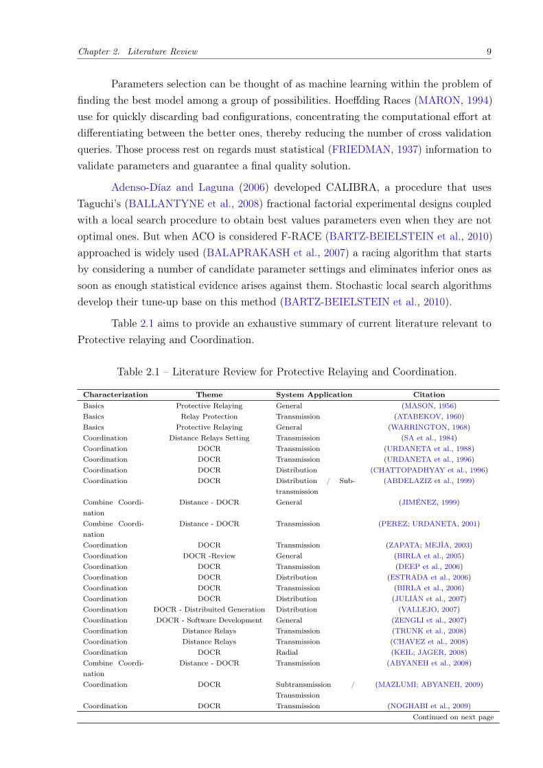
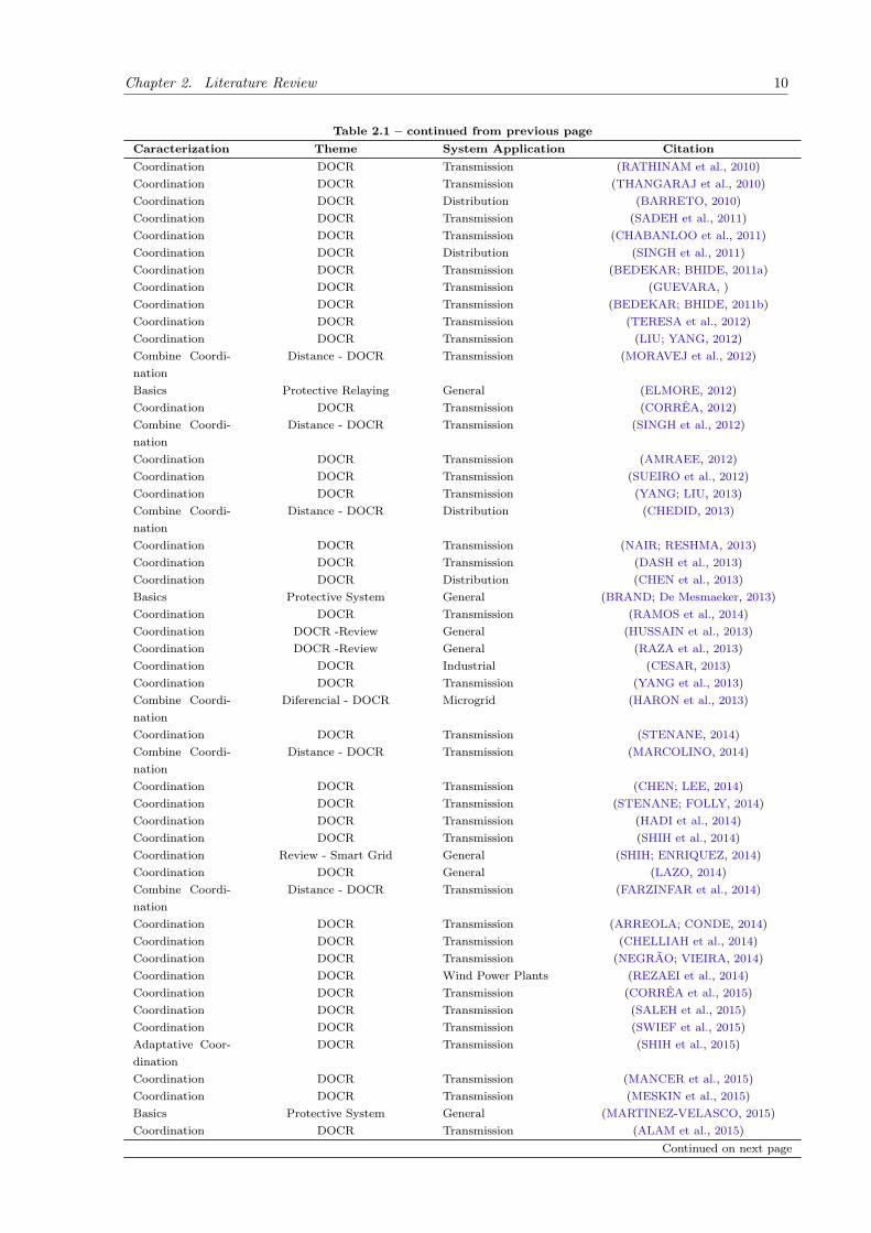
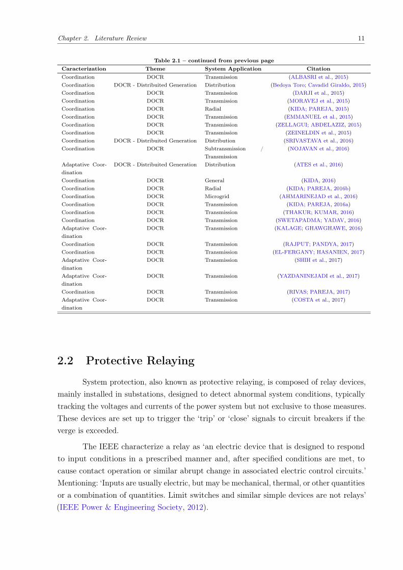
Table 2.1 aims to provide an exhaustive summary of current literature relevant toProtective relaying and Coordination.
Table 2.1 – Literature Review for Protective Relaying and Coordination.
Characterization Theme System Application CitationBasics Protective Relaying General (MASON, 1956)Basics Relay Protection Transmission (ATABEKOV, 1960)Basics Protective Relaying General (WARRINGTON, 1968)Coordination Distance Relays Setting Transmission (SA et al., 1984)Coordination DOCR Transmission (URDANETA et al., 1988)Coordination DOCR Transmission (URDANETA et al., 1996)Coordination DOCR Distribution (CHATTOPADHYAY et al., 1996)Coordination DOCR Distribution / Sub-
transmission(ABDELAZIZ et al., 1999)
Combine Coordi-nation
Distance - DOCR General (JIMÉNEZ, 1999)
Combine Coordi-nation
Distance - DOCR Transmission (PEREZ; URDANETA, 2001)
Coordination DOCR Transmission (ZAPATA; MEJÍA, 2003)Coordination DOCR -Review General (BIRLA et al., 2005)Coordination DOCR Transmission (DEEP et al., 2006)Coordination DOCR Distribution (ESTRADA et al., 2006)Coordination DOCR Transmission (BIRLA et al., 2006)Coordination DOCR Distribution (JULIÁN et al., 2007)Coordination DOCR - Distribuited Generation Distribution (VALLEJO, 2007)Coordination DOCR - Software Development General (ZENGLI et al., 2007)Coordination Distance Relays Transmission (TRUNK et al., 2008)Coordination Distance Relays Transmission (CHAVEZ et al., 2008)Coordination DOCR Radial (KEIL; JAGER, 2008)Combine Coordi-nation
Distance - DOCR Transmission (ABYANEH et al., 2008)
Coordination DOCR Subtransmission /Transmission
(MAZLUMI; ABYANEH, 2009)
Coordination DOCR Transmission (NOGHABI et al., 2009)Continued on next page
Chapter 2. Literature Review 10
Table 2.1 – continued from previous pageCaracterization Theme System Application CitationCoordination DOCR Transmission (RATHINAM et al., 2010)Coordination DOCR Transmission (THANGARAJ et al., 2010)Coordination DOCR Distribution (BARRETO, 2010)Coordination DOCR Transmission (SADEH et al., 2011)Coordination DOCR Transmission (CHABANLOO et al., 2011)Coordination DOCR Distribution (SINGH et al., 2011)Coordination DOCR Transmission (BEDEKAR; BHIDE, 2011a)Coordination DOCR Transmission (GUEVARA, )Coordination DOCR Transmission (BEDEKAR; BHIDE, 2011b)Coordination DOCR Transmission (TERESA et al., 2012)Coordination DOCR Transmission (LIU; YANG, 2012)Combine Coordi-nation
Distance - DOCR Transmission (MORAVEJ et al., 2012)
Basics Protective Relaying General (ELMORE, 2012)Coordination DOCR Transmission (CORRÊA, 2012)Combine Coordi-nation
Distance - DOCR Transmission (SINGH et al., 2012)
Coordination DOCR Transmission (AMRAEE, 2012)Coordination DOCR Transmission (SUEIRO et al., 2012)Coordination DOCR Transmission (YANG; LIU, 2013)Combine Coordi-nation
Distance - DOCR Distribution (CHEDID, 2013)
Coordination DOCR Transmission (NAIR; RESHMA, 2013)Coordination DOCR Transmission (DASH et al., 2013)Coordination DOCR Distribution (CHEN et al., 2013)Basics Protective System General (BRAND; De Mesmaeker, 2013)Coordination DOCR Transmission (RAMOS et al., 2014)Coordination DOCR -Review General (HUSSAIN et al., 2013)Coordination DOCR -Review General (RAZA et al., 2013)Coordination DOCR Industrial (CESAR, 2013)Coordination DOCR Transmission (YANG et al., 2013)Combine Coordi-nation
Diferencial - DOCR Microgrid (HARON et al., 2013)
Coordination DOCR Transmission (STENANE, 2014)Combine Coordi-nation
Distance - DOCR Transmission (MARCOLINO, 2014)
Coordination DOCR Transmission (CHEN; LEE, 2014)Coordination DOCR Transmission (STENANE; FOLLY, 2014)Coordination DOCR Transmission (HADI et al., 2014)Coordination DOCR Transmission (SHIH et al., 2014)Coordination Review - Smart Grid General (SHIH; ENRIQUEZ, 2014)Coordination DOCR General (LAZO, 2014)Combine Coordi-nation
Distance - DOCR Transmission (FARZINFAR et al., 2014)
Coordination DOCR Transmission (ARREOLA; CONDE, 2014)Coordination DOCR Transmission (CHELLIAH et al., 2014)Coordination DOCR Transmission (NEGRÃO; VIEIRA, 2014)Coordination DOCR Wind Power Plants (REZAEI et al., 2014)Coordination DOCR Transmission (CORRÊA et al., 2015)Coordination DOCR Transmission (SALEH et al., 2015)Coordination DOCR Transmission (SWIEF et al., 2015)Adaptative Coor-dination
DOCR Transmission (SHIH et al., 2015)
Coordination DOCR Transmission (MANCER et al., 2015)Coordination DOCR Transmission (MESKIN et al., 2015)Basics Protective System General (MARTINEZ-VELASCO, 2015)Coordination DOCR Transmission (ALAM et al., 2015)
Continued on next page
Chapter 2. Literature Review 11
Table 2.1 – continued from previous pageCaracterization Theme System Application CitationCoordination DOCR Transmission (ALBASRI et al., 2015)Coordination DOCR - Distribuited Generation Distribution (Bedoya Toro; Cavadid Giraldo, 2015)Coordination DOCR Transmission (DARJI et al., 2015)Coordination DOCR Transmission (MORAVEJ et al., 2015)Coordination DOCR Radial (KIDA; PAREJA, 2015)Coordination DOCR Transmission (EMMANUEL et al., 2015)Coordination DOCR Transmission (ZELLAGUI; ABDELAZIZ, 2015)Coordination DOCR Transmission (ZEINELDIN et al., 2015)Coordination DOCR - Distribuited Generation Distribution (SRIVASTAVA et al., 2016)Coordination DOCR Subtransmission /
Transmission(NOJAVAN et al., 2016)
Adaptative Coor-dination
DOCR - Distribuited Generation Distribution (ATES et al., 2016)
Coordination DOCR General (KIDA, 2016)Coordination DOCR Radial (KIDA; PAREJA, 2016b)Coordination DOCR Microgrid (AHMARINEJAD et al., 2016)Coordination DOCR Transmission (KIDA; PAREJA, 2016a)Coordination DOCR Transmission (THAKUR; KUMAR, 2016)Coordination DOCR Transmission (SWETAPADMA; YADAV, 2016)Adaptative Coor-dination
DOCR Transmission (KALAGE; GHAWGHAWE, 2016)
Coordination DOCR Transmission (RAJPUT; PANDYA, 2017)Coordination DOCR Transmission (EL-FERGANY; HASANIEN, 2017)Adaptative Coor-dination
DOCR Transmission (SHIH et al., 2017)
Adaptative Coor-dination
DOCR Transmission (YAZDANINEJADI et al., 2017)
Coordination DOCR Transmission (RIVAS; PAREJA, 2017)Adaptative Coor-dination
DOCR Transmission (COSTA et al., 2017)
2.2 Protective Relaying
System protection, also known as protective relaying, is composed of relay devices,mainly installed in substations, designed to detect abnormal system conditions, typicallytracking the voltages and currents of the power system but not exclusive to those measures.These devices are set up to trigger the ‘trip’ or ‘close’ signals to circuit breakers if theverge is exceeded.
The IEEE characterize a relay as ‘an electric device that is designed to respondto input conditions in a prescribed manner and, after specified conditions are met, tocause contact operation or similar abrupt change in associated electric control circuits.’Mentioning: ‘Inputs are usually electric, but may be mechanical, thermal, or other quantitiesor a combination of quantities. Limit switches and similar simple devices are not relays’(IEEE Power & Engineering Society, 2012).

Chapter 2. Literature Review 12
2.2.1 Power System Protection Components
Power line
Transmission line parameters are evenly distributed along the line length, and someof them are also functions of frequency. For steady-state studies, such as short-circuitcalculations, positive- and zero-sequence parameters calculated at the power frequencyfrom tables and simple handbook formulas may suffice (MARTINEZ-VELASCO, 2015).
Source and Generation
Source models used in protection studies are represented by means of detailedmachine models or as ideal sinusoidal sources behind subtransient reactances or theequivalent Thevenin impedances of the system. The choice of a specific model depends onsystem configuration, the location of the fault and the objectives of the study (MARTINEZ-VELASCO, 2015).
Power Transformer
Transformer modelling over a wide frequency range still presents substantial difficul-ties: the transformer inductances are nonlinear and frequency dependent, the distributedcapacitances between turns, between winding segments and between windings and groundproduce resonances that can affect the terminal and internal transformer voltages.
Circuit Breaker
Circuit breakers are usually represented as ideal switches; that is, the switch opensat a current zero and there is no representation of arc dynamics and losses. Custom-madecircuit breaker models can be employed for detailed arc modelling. The types of switchesthat are applicable for protection studies are presented below.
2.2.2 Instrument Transformers
The main tasks of instrument transformers are:
• To transform currents or voltages from usually a high value to a value easy to handlefor relays and instruments.
• To insulate the relays, metering, and instruments from the primary high-voltagesystem.
• To provide possibilities of standardizing the relays and instruments, etc. to a fewrated currents and voltages.
IEEE Std C57.13-2016 Requirements for Instrument Transformers, InternationalElectrotechnical Commission (IEC) 61869 2007-2016 Instrument transformers are most

Chapter 2. Literature Review 13
recent standards to newly manufactured instrument transformers with analog or digitaloutput for use with electrical measuring instruments or electrical protective devices.
Voltage transformers
There are basically, two types of voltage transformers used for protective equipment.
1. Electromagnetic type (commonly referred to as a voltage transformer (VT))
2. Capacitor type (referred to as a capacitor voltage transformer (CVT))
The electromagnetic type is a step-down transformer whose primary and secondarywindings are connected with a number of turns in a winding which is directly proportional tothe open-circuit voltage being measured or produced across it. This type of electromagnetictransformers is used in voltage circuits up to 110/132 kV. For still higher voltages, it iscommon to adopt the second type namely the CVT (HEWITSON et al., 2005).
Accuracy of voltage transformers
The voltage transformers shall be capable of producing secondary voltages, whichare proportionate to the primary voltages over the full range of input voltage expectedin a system. Voltage transformers for protection are required to maintain reasonablygood accuracy over a large range of voltage from 0 to 173% of normal. However, theclose accuracy is more relevant for metering purposes, while for protection purposes themargin of accuracy can be comparatively less (HEWITSON et al., 2005). Under transientconditions VTs and CVTs can be subjected to ferroresonance. This phenomenon leadsto overvoltages, which can lead to misoperation and (thermal and dielectric) failure(MARTINEZ-VELASCO, 2015). Permissible errors vary depending on the burden andpurpose of use and typical values as per IEC are as follows.
Current transformers
All current transformers used in protection are basically similar in construction tostandard transformers in that they consist of magnetically coupled primary and secondarywindings, wound on a common iron core, the primary winding being connected in serieswith the network, unlike voltage transformers (HEWITSON et al., 2005). They must,therefore, withstand the networks short-circuit current.
There are two types of current transformers:
1. Wound primary type
2. Bar primary type

Chapter 2. Literature Review 14
The wound primary is used for the smaller currents, but it can only be applied onlow fault level installations due to thermal limitations as well as structural requirementsdue to high magnetic forces. For currents greater than 100 A, the bar primary type is usedconsidering that if the secondary winding is evenly distributed around the complete ironcore, its leakage reactance is eliminated. Protection current transformers (CTs) are mostfrequently of the bar primary, toroidal core with evenly distributed secondary windingtype construction.
Performance of instrument transformers under transient conditions have shown thefollowing areas of concern (MARTINEZ-VELASCO, 2015):
• CT saturation reduces the magnitude of the secondary current. The consequence forelectromechanical relays is a reduction of the operating force or torque; a reducedtorque increases the operation time and reduces the reach of the relay.
• CT saturation affects the zero-crossings of the current wave, and hence will affectschemes that depend on the zero crossings, such as phase comparators.
• The relaxation current in the CT secondary is the current that flows when theprimary circuit is de-energized. This current is more pronounced in the case of CTswith an anti-remnant air gap.
• The relaxation current can delay the resetting of low-set overcurrent relays and alsocause the false operation of breaker failure relays.
2.2.3 Zones of Protection
Protective relaying should be a part and parcel of overall system planning, design,and operation. Circuit breakers are to be located at appropriate places. The componentsor equipment and parts of the system to be protected by the circuit breakers must beclearly identified (MURTY, 2017).
Fig. 2.1 illustrates such an identification and demarcation of zones. Overlappingof the zones may be observed. Each zone generally covers one or two of power systemelements. Location of current transformers determines the boundaries of the zones. This ispurely from the protection point of view only.
A correct zoning should take into account:
• No point in the electrical system should be unprotected.
• All types of short circuits within the zone, including the edge, must be viewed bythe appropriate detector elements (Reliability, Sensitivity, and Speed).

Chapter 2. Literature Review 15
Figure 2.1 – Zones of Protection
• Any type of short circuit outside a zone should be seen by its detector elements butnot activate tripping devices. (Selectivity)
The protection zone determines the selection of unitary or no unitary protectionschemes, which define an absolute selectivity and are constituted by the backup protections.
2.2.4 Protection system philosophies
There are two main protection philosophies to which all protection systems adhere.
Unit protection
The philosophy of unit protection defines that the protection system should onlydetect and react to primary system faults within the zone of protection while remaininginoperative for external faults. The protection scheme illustrated in Fig. 2.2 represents asimple unit protection scheme (BOOTH; BELL, 2013; DAVIES, 1998).
Figure 2.2 – Unit protection system (current differential protection)
Unit schemes typically involve protection relays that monitor the primary systemconditions at each end, or boundary, of the protected zone. The relays measure some

Chapter 2. Literature Review 16
parameter and perform a comparison with the parameter being measured by the otherrelay within the unit scheme. If some threshold criterion is violated, for example, themeasured currents are not equal or the vector summation of the measured currents is notequal to zero, then the protection relay initiate the process which will lead to isolation ofthe plant within the protected zone (SARKAR, 2015). Because of this requirement forcomparison of parameters from each ’end’ of the protected zone, almost all unit protectionschemes have a requirement for relay-to-relay communications facilities, which may beachieved using a number of methods. For the system above, the zone of protection is clearlydefined. To be exact, the zone of detection is between the measurement points, while thezone of protection is between the circuit breakers; normally, the CTs and circuit breakersare at almost identical locations. If, for example, each relay in the system form Fig 2.2 wascomparing the magnitude of its measured current with the other relay’s measured current,then for Fault 1, the currents will not be equal and the relays will trip. For the case of Fault2, while both measured currents will be far in excess of normal load current levels, theywill still be equal, and the protection relays should remain stable. Unit protection systemsoffer high levels of discrimination and stability, ensuring that the protection system onlyoperates for faults within the protected zone, while remaining are inoperative for ’external’faults. The main negative aspect associated with unit schemes is that they do not possessbackup protection capabilities, and there is a considerable expense associated with theuse of communications. Furthermore, reliance on communications for operation gives riseto concern over the reliability of the communications link, which is sometimes addressedthrough the use of multiple communications systems, further increasing costs. The lack ofbackup capabilities is usually addressed through the use of non-unit schemes in additionto the unit scheme.
Non-unit protection
The protection scheme arrangement presented in Fig. 2.3 represents a simple non-unit protection scheme. The main difference between unit and non-unit schemes is thatindividual non-unit schemes do not independently protect one clearly defined zone of thesystem (BOOTH; BELL, 2013).
Figure 2.3 – Non-unit protection system (overcurrent protection)
In Fig. 2.3, the zone of protection, certainly covers Fault 1, but in this case, the‘zone’ gradually ‘fades’ on the second line and, for Fault 2, it appears that the protection

Chapter 2. Literature Review 17
may provide coverage, but in the case above, this is not certain. The ‘reach’ of non-unitschemes can be varied by altering the settings on the relay, but non-unit schemes invariablyexhibit characteristics whereby the reaction of the protection system varies as the locationof the fault changes. In the example above, if the protection relay was an overcurrentrelay, then it will operate quickly for Fault 1, but with an increasing time delay as thefault location moved further along the system to the right, operating with a relativelylong time delay for Fault 2, and ceasing to operate as the fault moved further alongLine 2. Impedance, or distance protection, is also a non-unit scheme, but rather than acontinuously decreasing operation time, it exhibits a stepped characteristic, operating withfixed delays as the fault position moves from one zone to another in terms of its distancefrom the relay’s measurement point.
Figure 2.4 – Overlapping zone of protection in a non-unit arrangement (overcurrent pro-tection)
Adjacent non-unit protection schemes on an interconnected power system havean element of overlap with respect to their respective zones of protection as shown inFig. 2.4. This overlap is useful for providing backup protection in the event of failureof one element of the overall protection system. However, the criterion of selectivity, ordiscrimination, must still be satisfied and the non-unit scheme closest to the fault shouldalways trip before any other non-unit schemes, which must remain stable until the closestschemes have operated, only operating if the primary protection fails to operate. Non-unitschemes, when compared to unit schemes, do not offer such high levels of discriminationand stability, but, as already mentioned, provide valuable backup protection capabilities.
2.2.5 Primary and backup protection
Every zone identified for protection will have a suitable protection specified. If afault occurs in that zone, it is the duty of the relays in that zone to identify and isolate thefaulty element in that zone. The relay in that zone will be designated as the primary relay.If for what so ever reason this primary relay fails to operate, there should be a second lineof defense called backup protection. The relay in the backup protection is set to operateafter a predetermined delay time given to primary relay so that continued existence of thefault in the system may not cause serious trouble (BAYLISS; HARDY, 2007; MURTY,2017).

Chapter 2. Literature Review 18
It is understood from the above that when primary protection fails, the backup orsecondary protection operates and saves the system. But, then a large part of the systemmay get isolated in such an event. This cannot be avoided.
2.2.6 Protection techniques
Using measurement inputs from CTs and VTs, protection relays detect the presenceof a fault on the system using a number of techniques. Unit and non-unit are used, inparallel, at transmission levels to provide high levels of discrimination and stability fromthe unit schemes, with the backup being provided by non-unit schemes, although itis important to emphasize that non-unit schemes can also operate extremely quickly,depending on the settings employed. At distribution and consumer voltage levels, non-unitschemes are normally employed (BOOTH; BELL, 2013).
Current Relays
The following types of current relays are normally considered into actual transmis-sion power systems:
• Plain overcurrent and/or earth fault relay with an inverse definite minimum time(IDMT) interval or definite time (DT) delay characteristics.
• Overcurrent and/or earth fault relay as above but including directional elements.Note that a directional overcurrent relay requires a voltage connection and is nottherefore operated by current alone.
• Instantaneous overcurrent and/or earth fault relays. For example, a high set overcur-rent (HSOC) relay.
• Sensitive earth fault (SEF) relays.
As the name suggests, this method is based on measurement of current magnitudes,and a fault may be deemed to exist when the measured current exceeds a predeterminedthreshold level.
Historically this type of relay characteristic has been produced using electromagneticrelays, and many such units still exist in power systems. A metal disc is pivoted so as to befree to rotate between the poles of two electromagnets each energized by the current beingmonitored. The torque produced by the interaction of fluxes and eddy currents inducedin the disc is a function of the current. The disc speed is proportional to the torque. Asoperating time is inversely proportional to speed, operating time is inversely proportionalto a function of current (see Figure 2.5). The disc is free to rotate against the restrainingor resetting torque of a control spring. Contacts are attached to the disc spindle and under
Chapter 2. Literature Review 19
preset current levels operate to trip, via the appropriate circuitry, the required circuitbreaker(BAYLISS; HARDY, 2007).
Figure 2.5 – Simplified time-current characteristic of standard inverse overcurrent protec-tion
Current relay application
• Radial network: Consider from individual industrial application to distribution powersystem, reliable depending exclusively on a CT connection.
• Meshed network: The use of inverse time overcurrent relays on a meshed systemrequires the use of directional relays at all points where fault current could flowin both directions. A directional relay is merely a combination of the inverse timeovercurrent relay and a directional sensing unit.
IDMT backup protection
In more important networks and at higher voltage levels current relays are used asa ‘back-up’ to more sophisticated and faster acting ‘main’ protection systems. The backupprotection should be graded to achieve selective tripping if the main protection fails tooperate. However, it must be noted that this is not always possible on highly interconnectednetworks involving widespread generation sources(BAYLISS; HARDY, 2007). Figure 2.6shows a simple relay scheme for a transmission line where relay A (Backup) and relayB (Primary) should be coordinated based on their operation curve (Figure 2.7), wherebetween both curves must respect the coordination time interval .

Chapter 2. Literature Review 20
Figure 2.6 – Overcurrent protection for two serially connected feeders
Figure 2.7 – Time-current characteristics with settings and fault currents for two coordi-nated overcurrent relays
Instantaneous HSOC relays
The tripping times at high fault levels associated with the IDMT characteristicmay be shortened by the addition of instantaneous HSOC elements. These may be anintegral part, for optional use depending upon front panel settings, of a modern solid staterelay (BAYLISS; HARDY, 2007).
Distance relays
Designed to respond to current, voltage, and the phase angle between the currentand voltage. These quantities can be used to compute the impedance seen by the relay.which is proportional to the distance to the fault (ANDERSON, 1999).
Early applications of distance protection utilized relay operating times that were afunction of the impedance for the fault. The nearer the fault, the shorter the operatingtime. This has the same disadvantages as overcurrent protection, the grading settings maylead to tripping times that are too long to prevent damage and service interruption, andthat satisfactory grading for complex networks is quite difficult to attain (EL-HAWARY,1995).

Chapter 2. Literature Review 21
Present practice is to set the relay to operate simultaneously for faults that occurin the first 80 percent of the feeder length (known as the first zone). Faults beyond thispoint and up to a point midway along the next feeder are cleared by arranging for thezone setting of the relay to be extended from the first zone value to the second zone valueafter a time delay of about 0.5 to 1 second. The second zone for the first relay shouldnever be less than 20 percent of the first feeder length. The zone setting extension is doneby increasing the impedance in series with the relay voltage coil current. A third zone isprovided (using a starting relay) extending from the middle of the second feeder into thethird feeder up to 25 percent of the length with a further delay of 1 or 2 seconds. Thisprovides backup protection as well (EL-HAWARY, 1995; ANDERSON, 2009).
Fig. 2.8 presents a simple distance protection scheme in terms of its zones ofprotection and the time delays associated with operation of the relay for faults detected ineach zone. Time definition for each zone usually depends on individual coordination of dis-tance or manufacturer recommendations (EL-HAWARY, 1995; THOMPSON; HEIDFELD,2015).
Figure 2.8 – Zones of protection of distance protection with indicative time delays ofoperation for faults detected in each zone.
Fig. 2.9 below illustrates the zone boundaries for each of the three zones in thecomplex impedance plane. The reason that the zone boundaries are circular is historical.When electromechanical relays were used, they effectively compared only the magnitudes(and not the relative phases) of the measured currents and voltages, and thus could onlydetermine the magnitude of the impedance, which equates to a circle when plotted in theimpedance plane. This circular characteristic is also a useful feature, as resistive faults canalso be detected to a certain degree. For example, if a fault in the middle of Line 1 had aresistive element, then the locus of the measured impedance may lie in the vicinity of thecross indicated in the figure, and will still be detected (BOOTH; BELL, 2013).

Chapter 2. Literature Review 22
Figure 2.9 – Illustration of distance protection zone boundaries in the complex impedanceplane.
2.2.7 Modernization of the Protection System
The microprocessor or digital relays offer many advantages and benefits over elec-tromechanical relays such as reduced installation and maintenance costs, applicationflexibility besides increasingly developed control and monitoring functions. But the use ofelectromechanical relays has not been abandoned because they still meet the protectionrequirements of electrical power systems, finance is still an important factor against increas-ing sophistication and number of functions and facilities that digital relays have offered toProtection Engineers and event analysis energy companies and industry (MADRIGAL;ULUSKI, 2015; AGUERO et al., 2017).
One of the main advantages related to the modernization of the relays is the inherentflexibility of the digital technology and the possibility of producing adaptive characteristicsand multiple adjustments to the system. The author Rufato Junior (2006) showed thefeasibility and technical and economic benefits of using digital relays, considering highinterruption rates caused by a fail in selectivity of the protections in the distributionsystem. In Brazil, Ribeiro and Goes (2013) shows a modernization of protection systems,a control, and supervision integration project presented with Companhia Paranaense deEnergia (COPEL).
Making better use of existing and new technologies can reduce costs and facilitatethe siting of transmission circuits. An accurate control of the system delivers an aptitudeto increase capacity and availability (U.S. DOE, 2015).

23
3 Mathematical Formulation
In this chapter, the problem of coordination is formulated as a mathematicaloptimization problem, containing an objective function, which is responsible for minimizingthe times of relay performance and a set of constraints. Both Distance and Overcurrentrelays are considered into formulation, as individuals or together. Studying also the spaceof solution for this problem.
3.1 Mathematical Modeling DOCR
An IDMT, a compromise worldwide popular curve, introduced about 1920 havebeen a satisfied solution. Theoretically, their time ordinates should be proportional to thetime dial setting (contact travel) so that, if the times for a given current were divided bythe time dial setting, all the curves should be coinciding. Unfortunately, the inertia of thedisc makes was impracticable at low current values because it takes a short time for thedisc to accelerate from standstill to its steady speed (WARRINGTON, 1968).
A solution for limiting this obstacle was publishing a family of curves, the inversetime overcurrent most common curves are the IEEE, IEC, GE Type family of overcurrentrelays from GE (IAC), and I2t standard curve shapes within their types shows in Tab. 3.1.
Table 3.1 – Overcurrent Relay Types
IEEE IEC GE TYPE IAC OTHERIEEE Extremely Inv. IEC Curve A IAC Extremely Inv. I2tIEEE Very Inverse IEC Curve B IAC Very Inverse FlexCurvesIEEE Moderately Inv. IEC Curve C IAC Inverse Recloser Curves
IEC Short Inverse IAC Short Inverse Definite Time
Before considering the setting of these relays, the following definitions will behelpful.
Time Dial Setting or Time Multiplier Setting. A means of adjusting the mobilebackstop which controls the driving of the disc and thereby varies the time in which therelay will close its contacts for given values of fault current.
Plug Setting, Pickup Current, or Tap Block. A device providing a range of currentsettings at which the relay will start to operate.
IDMT characteristics are selectable from a choice of curves conforming to thefollowing formula (GE Industrial Systems, 2009).

Chapter 3. Mathematical Formulation 24
3.1.1 IEEE Curves
The IEEE time overcurrent curve shapes conform to industry standards and theIEEE C37.112-1996 curve classifications for extremely, very, and moderately inverse. TheIEEE curves are derived from the formula:
t = TDS
(A
( IIpickup
)p − 1+B
)(3.1)
where t is operating time (in seconds), TDS Time Dial Setting, I input current,Ipickup Pickup Current setting and A, p, B are constant parameters.
Table 3.2 – IEEE Inverse Time Curve Constants
IEEE CURVE SHAPE A B pIEEE Extremely Inverse 28.2 0.1217 2IEEE Very Inverse 19.61 0.491 2IEEE Moderately Inverse 0.0515 0.114 0.02
3.1.2 IEC Curves
For European applications, the relay offers three standard curves defined in IEC255-4 and British standard BS142. These are defined as IEC Curve A, IEC Curve B, andIEC Curve C. The formula for these curves is:
t = TDS
(K
( IIpickup
)E − 1
)(3.2)
where t is operating time (in seconds), TDS Time Dial Setting, I input current,Ipickup Pickup Current setting and K, E are constant parameters.
Table 3.3 – IEC (BS) Inverse Time Curve Constants
IEC (BS) CURVE SHAPE K EIEC Curve A (BS142) 0.14 0.02IEC Curve B (BS142) 13.5 1IEC Curve C (BS142) 80 2IEC Short Inverse 0.05 0.04
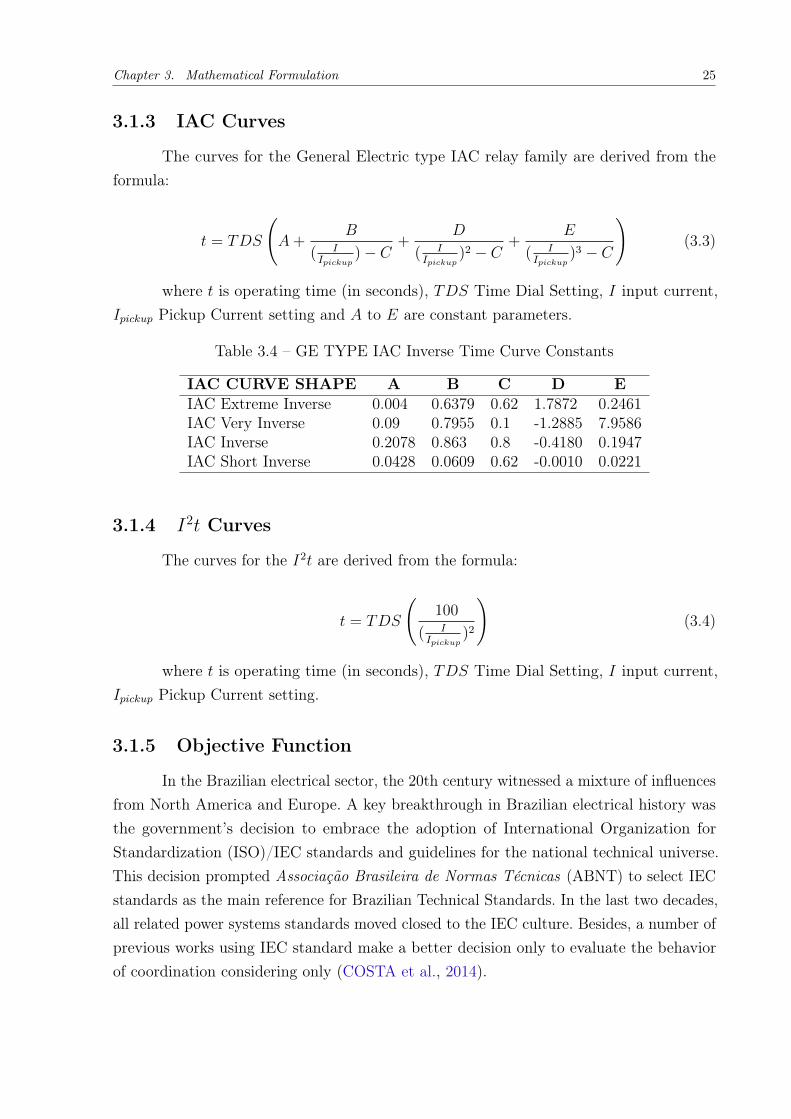
Chapter 3. Mathematical Formulation 25
3.1.3 IAC Curves
The curves for the General Electric type IAC relay family are derived from theformula:
t = TDS
(A+
B
( IIpickup
)− C+
D
( IIpickup
)2 − C+
E
( IIpickup
)3 − C
)(3.3)
where t is operating time (in seconds), TDS Time Dial Setting, I input current,Ipickup Pickup Current setting and A to E are constant parameters.
Table 3.4 – GE TYPE IAC Inverse Time Curve Constants
IAC CURVE SHAPE A B C D EIAC Extreme Inverse 0.004 0.6379 0.62 1.7872 0.2461IAC Very Inverse 0.09 0.7955 0.1 -1.2885 7.9586IAC Inverse 0.2078 0.863 0.8 -0.4180 0.1947IAC Short Inverse 0.0428 0.0609 0.62 -0.0010 0.0221
3.1.4 I2t Curves
The curves for the I2t are derived from the formula:
t = TDS
(100
( IIpickup
)2
)(3.4)
where t is operating time (in seconds), TDS Time Dial Setting, I input current,Ipickup Pickup Current setting.
3.1.5 Objective Function
In the Brazilian electrical sector, the 20th century witnessed a mixture of influencesfrom North America and Europe. A key breakthrough in Brazilian electrical history wasthe government’s decision to embrace the adoption of International Organization forStandardization (ISO)/IEC standards and guidelines for the national technical universe.This decision prompted Associação Brasileira de Normas Técnicas (ABNT) to select IECstandards as the main reference for Brazilian Technical Standards. In the last two decades,all related power systems standards moved closed to the IEC culture. Besides, a number ofprevious works using IEC standard make a better decision only to evaluate the behaviorof coordination considering only (COSTA et al., 2014).

Chapter 3. Mathematical Formulation 26
Eq. 3.5 is an extension of the Eq. 3.2 evaluating operating time of the DOCRs evenwhen they are use as main or backup protection.
tik = TDSi
(K
( IikIpickup
)E − 1
)(3.5)
where tik is the operating time of the relay i for a fault in k, TDSi Time DialSetting for the relay i, Iik input current from a fault k seen by relay i, Ipickup PickupCurrent setting and K, E are constant parameters.
The concept of relay pickup tap setting could be formulated by
PSi =IpickupCTRi
(3.6)
where Ipickup is the primary pickup current and CTRi stands for the CT ratio. Pickupcurrent should be above maximum load current ensuring that relay does not trip on normalload conditions, normally with values within a continuous range but when related to PSdepends on relay’s available settings (continuous or discrete).
DOCR coordination problem can be stated as a parametric optimization problem,where the objective function (OF) to be minimized is the sum of the operating times ofthe relays connected to the system, subject to the following constraints (URDANETA etal., 1988).
This problem can be formulated mathematically as
minn∑i=1
n∑k=1
tik (3.7)
where tik is the operating time of the primary relay i for a fault k
3.1.6 Coordination Constraints
Coordination criteria (Selectivity Constraint) A fault is sensed by both primaryas well as secondary relay together. To avert violation in operation, the backup relay(BR) should take over the tripping action only after primary relay (PR) flops to operate(MANSOUR et al., 2007). If Ri is the primary relay for defect at k, and Rj is backup relayfor the same fault, next the coordination constraint can be seated as:
tj,k − ti,k = 4t (3.8)

Chapter 3. Mathematical Formulation 27
Where ti,k is the operating time of the primary relay Ri , for fault at k; tj,k is theoperating time for the backup relay Rj , for the same fault at k, 4t is the coordinationtime interval (CTI)
Bounds on TDS of each relay
TDSmini ≤ TDSi ≤ TDSmaxi (3.9)
TDSmini and TDSmaxi are minimum and maximum value of TDS of relay Ri, andTDSi in continuous domain.
Bounds on pickup current Ipickup setting of each relay
Iminpickup ≤ Ipickup ≤ Imaxpickup (3.10)
Iminpickup and Imaxpickup are minimum and the maximum value of pickup current settingof each relay, and Ipickup in continuous domain but when convert to PS may be discrete orcontinuous.
The range for all parameters is defined by the network topologies, manufacturerrecommendations, and standards limits and are individually described for each problempropose in this work.
3.2 Mathematical Modeling DOCR & Distance
Transmission and sub-transmission systems normally have a mixed scheme withDOCR and distance relays. Considering a pair of this relays for each circuit breaker,distance zones definition have an important matter in coordination. Distance relay zone-1has an instantaneous trip, been faster than DOCR units considered in this formulation;fact defining DOCR as the backup for Zone 1 for a distance relay (DZ-1) relays in certainfault locations. This approach is normally not considered due to fault location dependenceto configure zones on distance relays. For example, last resolution would be valid fornear-end and half-end fault locations but dismissed for far-end faults, supposing zone-1 toan 80% of the line.
Examining zone-2 of distance relay requires fault location evaluation, as seen inFig. 3.1, with three faults location by line (near-end, midpoint, and far-end) and holdingDOCRs primary relays to all cases, the backup configuration has a different pondereddefinition.
Fig. 3.1 diagram shows how it should be guaranteed the selectivity for the relaysof overcurrent for all the faults, but how it changes for the relays of distance that has asa rear zone 2. At the beginning of the line, zone 2 of the distance relay located where

Chapter 3. Mathematical Formulation 28
Figure 3.1 – Critical fault locations for the coordination between overcurrent and distancerelays
you find the backup overcurrent relay. In the middle of the line, has no zone 2 of actingdistance relay (Normally configured between 80
3.2.1 Objective Function
Considering the primary actuation times of the overcurrent relays and the trippingtimes for zone 2 of the distance relays, the objective function for coordination combinedwith relays of distance is written as Eq 3.11.
minn∑i=1
(n∑k=1
tOCik + tZ2i
)(3.11)
where tOCik is the operating time of the primary DOCR i for a fault k and tZ2i is
the time defined for the second zone of each distance relay.
3.2.2 Coordination Constraints
Eq. 3.8, 3.9, and 3.10 are still valid for the mixed mathematical model. Constraintsconsidered in the scheme are increased by new conditions depending on fault location.
Near-end faults
Coming from the DOCR model where ROCi is the primary relay for a fault at k and
ROCj is the backup relay for the same fault, the second zone of the RD
j is priority backup

Chapter 3. Mathematical Formulation 29
relay. Meaning, three levels of protection, first, ROCi following RD
j and ROCj .
tZ2j − tOCi,k = 4t (3.12)
tOCj,k − tOCi,k = 4t (3.13)
Midpoint faults
There is a lack where the second zone for distance relays is not under the protectionscheme, according to 2.2.6 between 20% and 80% of the line only actual zone-1 andbackup from zone-3 of adjacent backup. Zone-3 is not considered in this work, that’s whyexclusively DOCR generates constraints in this case.
tOCj,k − tOCi,k = 4t (3.14)
Far-end faults
On the contrary for far-end fault location, the second zone of the RDi is priority
backup relay of the ROCi leaving ROC
j behind. Intending, three levels of protection asnear-end faults constraints.
tZ2i − tOCi,k = 4t (3.15)
tOCj,k − tOCi,k = 4t (3.16)
Bounds on TDS of each relay
tZ2i min ≤ tZ2
i ≤ tZ2i max (3.17)
tZ2i min and tZ2
i max are minimum and maximum value of tZ2i of relay Ri.
Zone-2 is set with an 18 (tZ2i min) to 36 (tZ2
i max) cycles delay to coordinate withremote relays (THOMPSON; HEIDFELD, 2015). The remote relays use that time to clearthe fault and give breaker failure functions time to operate.
Table 3.5 – Distance relays second zone configuration time interval
Frequency Zone-2 set time (s)min max
Cycles 18 3650 Hz 0.36 0.7260 Hz 0.3 0.6

Chapter 3. Mathematical Formulation 30
3.3 Feasible Region and Problem Characterization
The coordination problem is formulated as mixed-integer nonlinear programming(MINLP) when TDS or PS are analyzed as discrete variables. Even considering both ascontinuous the relaxation maintains the nonlinear component into the problem. In meshednetworks, feasible region tends to a highly restricted hyperspace which does not support aconvex set. Nonconvex MINLPs are especially challenging because they contain nonconvexfunctions in the objective or the constraints, as seen in Fig. 3.2, the feasible region fora relay pair considering TDS fixed has nonconvex characteristics (Between point A andB there are points not contained in the feasible set); within a relaxation as Fig. 3.3 thesolution space has convex and linear but only consider one problem variable obtaining alocal optimum but certainly not a response closer to the global solution. In Fig. 3.4 a 3Dsurface plotting individual relay time considering TDS and PS variables.
Figure 3.2 – Feasible region for Primary-Backup Relay Considering TDS fixed.
Figure 3.3 – Feasible region for Primary-Backup Relay Considering PS fixed.
Solving nonconvex MINLPs may be replacing the nonconvex functions with convexpiecewise linear approximations and solve the corresponding approximation by usingmixed-integer linear programming solvers. Also, components of methods for directlysolving nonconvex MINLPs, generic tactics for reaching convex relaxations nonconvexfunctions or spatial branching can be used with these relaxations to get a convergentalgorithm (BELOTTI et al., 2012).
Some real-world applications cannot be solved to global optimality by using theprior methods discussed, because the problems are too large, generate a huge search tree,or like coordination must be solved in real time. In these situations, it is more desirableto obtain a good solution quickly than to wait for an optimal solution. Heuristic search
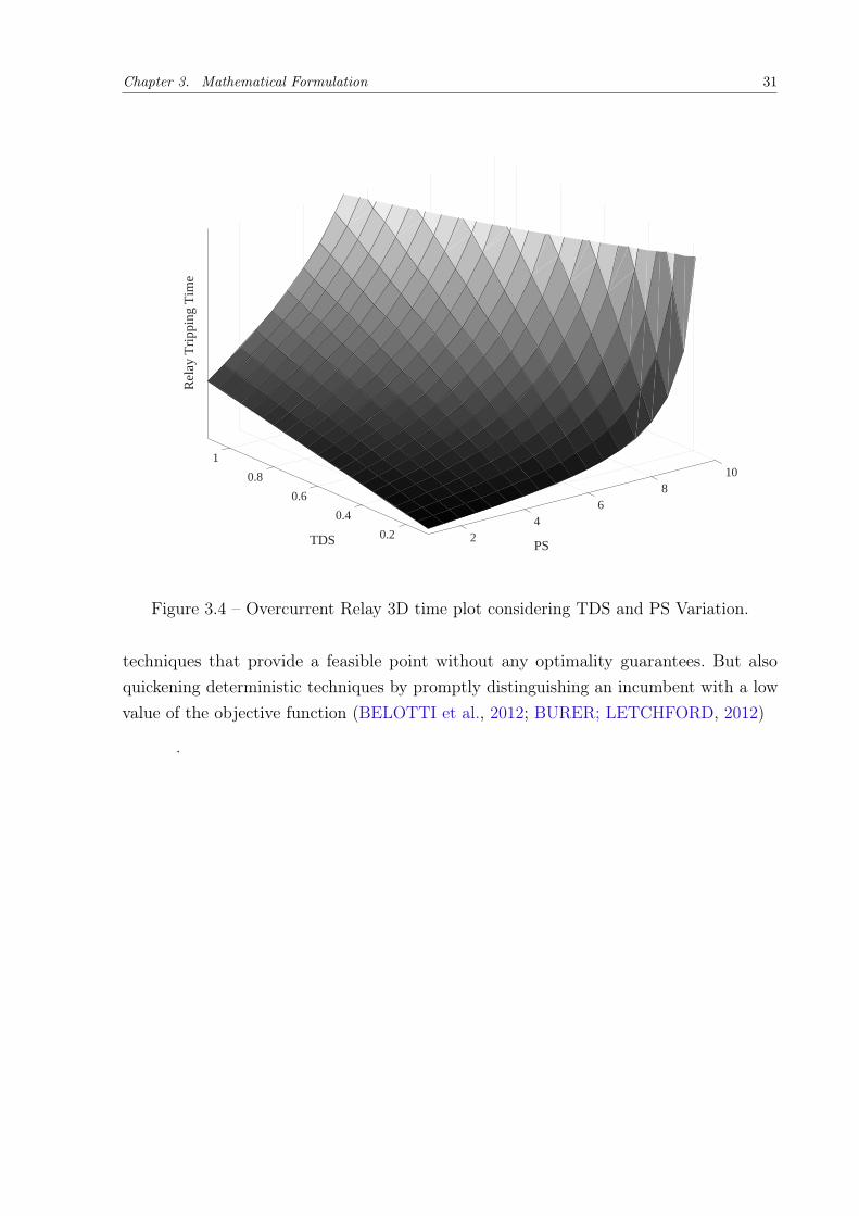
Chapter 3. Mathematical Formulation 31
1100.8
Rel
ay T
ripp
ing
Tim
e
8
TDS
0.6
PS
60.4 4
0.2 2
Figure 3.4 – Overcurrent Relay 3D time plot considering TDS and PS Variation.
techniques that provide a feasible point without any optimality guarantees. But alsoquickening deterministic techniques by promptly distinguishing an incumbent with a lowvalue of the objective function (BELOTTI et al., 2012; BURER; LETCHFORD, 2012)
.

32
4 Implementation
4.1 Ant Colony Optimization
The colonies of ants, and in general, insect societies, are distributed systems thatdespite the simplicity of their individuals have a highly structured social organization.The main idea is that these principles be exploited to coordinate populations of artificialagents that collaborate to solve computational problems. Ants coordinate their activitiesvia stigmergy, a form of indirect communication mediated by changes in the environment(DORIGO; STÜTZLE, 2004). The idea of ant algorithms is then to use a form of artificialstigma to coordinate societies of artificial agents.
Some considerations came from ants in the real world to inspire this technique.First, many ant species are almost blind, the communication between the ants is carriedout through a chemical called pheromone, and in some species, the pheromone is used tocreate paths (ant’s trails), see Fig. 4.1.
Figure 4.1 – Ants build solutions, that is, paths from a source to a destination node.
ACO algorithms for CO problems make use of a supposed pheromone model in orderto probabilistically construct solutions. A pheromone model consists of a set of numericalvalues, called pheromones, that is a function of the search experience of the algorithm(DORIGO; BLUM, 2005). The pheromone model is used to bias the solution constructiontoward regions of the search space enclosing high-quality solutions. An advantage formodel coordination problem using mixed ACO approach is a high probability of findingbetter solutions for actual systems.
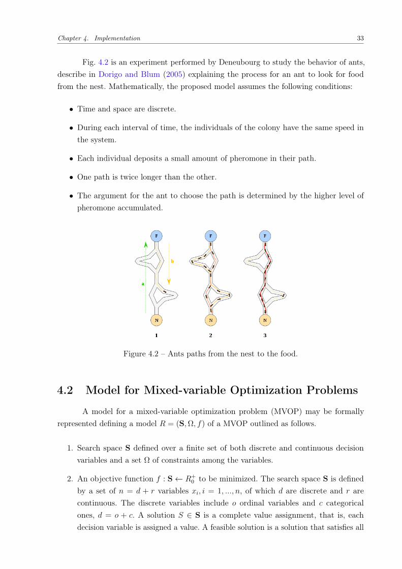
Chapter 4. Implementation 33
Fig. 4.2 is an experiment performed by Deneubourg to study the behavior of ants,describe in Dorigo and Blum (2005) explaining the process for an ant to look for foodfrom the nest. Mathematically, the proposed model assumes the following conditions:
• Time and space are discrete.
• During each interval of time, the individuals of the colony have the same speed inthe system.
• Each individual deposits a small amount of pheromone in their path.
• One path is twice longer than the other.
• The argument for the ant to choose the path is determined by the higher level ofpheromone accumulated.
Figure 4.2 – Ants paths from the nest to the food.
4.2 Model for Mixed-variable Optimization Problems
A model for a mixed-variable optimization problem (MVOP) may be formallyrepresented defining a model R = (S,Ω, f) of a MVOP outlined as follows.
1. Search space S defined over a finite set of both discrete and continuous decisionvariables and a set Ω of constraints among the variables.
2. An objective function f : S← R+0 to be minimized. The search space S is defined
by a set of n = d + r variables xi, i = 1, ..., n, of which d are discrete and r arecontinuous. The discrete variables include o ordinal variables and c categoricalones, d = o + c. A solution S ∈ S is a complete value assignment, that is, eachdecision variable is assigned a value. A feasible solution is a solution that satisfies all

Chapter 4. Implementation 34
constraints in the set Ω. A global optimum S∗ ∈ S is a feasible solution that satisfiesf(S∗) ≤ f(S) ∀S ∈ S. The set of all globally optimal solutions is denoted by S∗,S∗ ⊆ S . Solving an MVOP requires finding at least one S∗ ∈ S∗.
This method to tackle MVOPs combines a continuous relaxation and a categoricaloptimization approach. This strategy uses a categorical optimization approach to directlyhandle discrete variables without a continuous relaxation and continuous variables arehandled by a continuous optimization method, without the need to handle dependencybetween variables belonging to different distributions avoiding to find sub-optimal solutions(SOLNON, 2007).
4.3 ACO for Mixed-variable Optimization Problems
Initially, is described the structure of the multivariable algorithm (Fig. 4.3). Then,how the probabilistic solution construction for continuous variables, and categoricalvariables, is developed respectively. During the construction process, ordinal choose isdismissed due to similar construction compare to continuous variables, using categoricalprocedure guarantee independent convergence during function evaluation.
4.3.1 Codification
Derivate from the mathematical model, chosen variables are TDS and PS parametrizedas Continuous and Categorical, respectively. Codification bases in the next structure:
Based on an array of Fig. 4.3, solution archive (SA) form k solutions of n variableseach. In association with each solution Sj is a quality function f(Sj), which from best toworst, sorts the array and defines a weight ωj calculated using a Gaussian function withmean related to rank and standard deviation depending on the size k of the SA and a q asa parameter of the algorithm.
Quality Function = h1
n∑i=1
n∑k=1
tik + h2
nConst∑i=1
CV (4.1)
Where h1 and h2 are weighting factors for increasing or decreasing the influence offitness and unfitness function, respectively. Constraints violations (CV) is a time variablefor each violation.

Chapter 4. Implementation 35
Figure 4.3 – Structure of the solution archive used by ACOMV (SOLNON, 2007) In thiscase, reduced to two variable types.
4.4 Construction of a solution (an ant)
The process of building an alternative solution is basically a construction in whichelements are added gradually. The difference with classical heuristic methods lies in thefact that the added element is the product of learning, leaving behind the impact that theobjective function may have. Also, in order to generate a larger exploration of the solutionspace, the formation of feasible solutions is allowed.
In constructing an alternative solution by an ant algorithm it is essential to knowthe pheromone model, and whether the heuristic to guide the search for promising careerpaths based on information as possible. In addition, it is necessary to introduce an essentialcriterion for the construction of an alternative solution, which is neighborhood representedby a Gaussian Kernel as shows Fig. 4.4.
This type of construct algorithm is typically faster among approximate methods,the quality of the solutions they generate is often worst than the quality of the solutionsfound by local search algorithms.

Chapter 4. Implementation 36
Gaussian KernelIndividual Gaussian functions
Figure 4.4 – Gaussian Kernel of the SA
4.4.1 ACOMV Parameters
Construction for Continuous Variables
Continuous variables use the ant colony optimization for continuous domain (ACOR)algorithm (SOCHA; DORIGO, 2008) where an ant build probabilistically one solutionbased on the SA. Probability of designating a solution j is defined by his weight ωj in theSA (Figure 4.3) and ωl weight of all k solutions.
pj =ωj∑kl=1 ωl
(4.2)
After selection of jth solution, in order to attach a value to variable i, the antsamples the neighborhood over the value Ri
j of the chosen jth solution compare to all Ril
variables in the SA. The sampling is done using a normal probability density functionwith mean µ = Ri
j and standard deviation σ define by 4.3.
σ = ξk∑l=1
|Ril −Ri
j|k − 1
(4.3)
Parameter ξ has an important effect similar to pheromone persistence in the ACOfirst algorithm, with a particular impact on the convergence speed of the algorithm.
Construction for Categorical Variables
In this case, the PS variable could be treated as ordinal and use a relaxation ACOR
to solve it, but treating the PS variable as categorical is a guarantee for diversity, choosingfrom vector data.

Chapter 4. Implementation 37
Now, an ant choose between PS available values, probabilistically based on thenext equation:
pil =ωl∑PSi
j=1 ωj(4.4)
where ωl is the weight associated to each PS value, and calculated by:
ωl =
ωjl
uil+ q
ηif(η > 0, uil > 0)
ωjl
uilif(η = 0, uil > 0)
qη
if(η > 0, uil = 0)
(4.5)
Where ωjl is calculated according to 4.5. uil is the number of solutions that use PSifor the categorical variable i in the SA. η is the number of values from PS vector availableones that are not used by the SA. q has the same characteristics from the continuous part.
4.5 Restart Mechanism
The ACO algorithm is usually used with a restart strategy for struggling stagnationand avoiding local optimum. Always keeping the best-so-far solution in the SA. When anumber of successive iterations have a relative solution enhancement lower than certain εa restart is started (SOLNON, 2007). Normally, this strategy stands on generating a newSA only keeping the best-so-far, this work introduces a new restart technique using theparameter q increasing elitism of the algorithm.
4.6 Algorithm and Flowchart
A detailed Flowchart (see Fig. 4.5) for the algorithm implementation containingthe iterative process to find a solution.
The computational steps of ACO are given below based on (SOLNON, 2007):
4.7 Analysis of ACO parameters
Hard optimization problems often required algorithms which typically have severalparameters that need to be set or tuned such that some features of performance is optimized.Based on a statistical strategy for selecting the best configuration out of a set of candidateconfigurations under stochastic evaluations, F-Race is a racing algorithm for the taskof automatic algorithm configuration. This work uses an extension of the initial F-Race

Chapter 4. Implementation 38
Figure 4.5 – Flowchart for ACOMV
Algorithm 1 Outline of ACOMV
Initialize decision variablesInitialize and evaluate k solutionsSort solutions and store them in the archive SASA← Sort(S1Sk)while termination criterion is not satisfied doConstructAntSolutionfor 1 to m doProbabilistic Solution Construction for ACOR
Probabilistic Solution Construction for ACOMV C
Store and evaluate newly generated solutionsend forSort solutions and select the best k solutionsSA← Best(Sort(S1Sk))if σQF < ε thenApply Restart Strategy
end ifend while
algorithm, which leads to a family of algorithms called iterated F-Race implemented totuned up ACO algorithm.
4.7.1 F-RACE approach
Algorithms for tackling computationally complex problems have a number ofparameters that influence their search behavior. Many state-of-the-art algorithms cover
Chapter 4. Implementation 39
exact algorithms such as branch-and-bound algorithms, algorithm packages for integerprogramming, and relative algorithms such as stochastic local search (SLS) algorithms.The parameters can approximately be grouped into numerical and categorical parameters.
Examples of numerical parameters are the tabu tenure in tabu search algorithmsor the pheromone evaporation rate in ACO algorithms. Moreover, many algorithms can beseen as being composed of a set of specific components that are frequently interchangeable.Examples are diverse branching maneuverings in branch-and-bound algorithms, differenttypes of crossover operators in evolutionary algorithms, and different types of localsearch algorithms in iterated local search. These intervariable elements are frequentlywell expressed as categorical parameters of the underlying search method. Analysis hasdefinitely shown that the performance of parameterized algorithms depends strongly onthe particular values of the parameters, and the choice of a suitable setting of theseparameters is itself a challenging optimization problem (ADENSO-DÍAZ; LAGUNA, 2006;BIRATTARI, 2005; BIRATTARI et al., 2002).
Typically not only the setting of numerical parameters but also that of categoricalparameters needs to be settled, many state-of-the-art refers to an algorithm configurationproblem. An essential aspect of this problem is that it is typically a stochastic problem.Actually, there are two main sources of Ergodicity. The first is that often the algorithmitself is stochastic because it uses some randomized arrangements during the search. Infact, this stochasticity is typical for SLS algorithms (HOOS; STÜTZLE, 2005).
However, even if an algorithm is deterministic, its performance and search behaviordepend on the circumstantial instance to which it is applied. In fact, the particular instancebeing tackled can be seen as having been described according to some underlying, possiblyunknown probability distribution, adding in this way a second stochastic factor.
Hoeffding races (MARON; MOORE, 1993; MARON, 1994), an accelerating modelselection search for classification and function approximation, is an important racingalgorithm in machine learning which inspires methods like F-Race method convenientfor dealing with the stochastic characteristics of the ACO algorithm. The basic idea ofracing methods, in general, and this method in particular, is to evaluate a distributed setof candidate configurations iteratively on a succession of instances. As soon as enoughstatistical evidence is deduced against some candidate configurations, these are filteredand the race continues only with the surviving ones. In our case, this method uses aftereach evaluation round of the candidate arrangements the nonparametric Friedman test(FRIEDMAN, 1937) as a family-wise test: it checks whether there is confirmation that atleast one of the configurations is significantly different from others. If the null hypothesisof no differences is rejected, Friedman post-tests are applied to eliminate those candidateconfigurations that are significantly worse than the best one.

Chapter 4. Implementation 40
4.7.2 Algorithm Configuration Problem
F-Race is a pre-process to obtain an offline configuration of parameterized algo-rithms. In the training phase of offline tuning, an algorithm configuration is to be settledin a limited quantity of time that optimizes some pattern of algorithm performance. Thefinal algorithm configuration is then expanded in a production phase where the algorithmis used to solve earlier undiscovered instances. A significant aspect of this algorithmconfiguration problem is that it is a problem of generalization, as occurs in other disciplinessuch as machine learning. Based on a given set of training instances, the goal is to findhigh-performing algorithm configurations that perform well on (a probably infinite set of)unseen instances that are not available when deciding on the algorithm’s parameters. Hence,one conjecture that is tacitly done is that the set of training instances is representativeof the instances the algorithm faces once it is employed in the production phase. Theawareness of best performance or generalization is made explicit in the formal sense of thealgorithm configuration problem.
The problem of configuring a parameterized algorithm can be properly defined asa 7-tuple 〈Θ, I, pI , pC , t, C, T 〉 where:
• Θ is the possibly infinite set of candidate configurations.
• I is the possibly infinite set of instances.
• pI is a probability measure over the set I.
• t : I → < is a function associating to every instance the computation time that isallocated to it.
• c(θ, i, t, t(i)) is a random variable representing the cost measure of a configurationθ ∈ Θ on instance i ∈ I when run for computation time t(i).
• C ⊂ < is the range of c, that is, the possible values for the cost measure of theconfiguration θ ∈ Θ on an instance i ∈ I.
• pC is a probability measure over the set C: With the notation pC(c|θ, i) we indicatethe probability that c is the cost of running configuration θ on instance i.
• C(θ) = C(θ|Θ, I, pI , pC , t) is the criterion that needs to be optimized with respect toθ. In the most general case it measures in some sense the desirability of θ .
• T is the total amount of time available for experimenting with the given candidateconfigurations on the available instances before delivering the selected configuration.

Chapter 4. Implementation 41
On the basis of these concepts, solving the problem of configuring a parameterizedalgorithm is to find the configuration θ such that
θ = arg minθ∈Θ
C(θ) (4.6)
consider for C the expected value of the cost measure c
C(θ) = EI,C(c) =
∫∫c dpC(c|θ, i)dpI(i) (4.7)
where the expectation is considered with respect to both pI and pC , and theintegration is taken as defined by Bartz-Beielstein et al. (2010).
4.7.3 Iterated F-Race Algorithm
This implementation is based on the previous published by Balaprakash et al.(2007) and Bartz-Beielstein et al. (2010). However, it changes in some parameter choicesand extends the earlier version by defining a way to handle categorical parameters.
The number of iterations. Denoted by L the number of iterations of Iterated F-RaceAlgorithm (I/F-Race), and increase L with d, the number of parameters, using a set ofL = 2 + round(log2d).
Computational budget at each iteration. The computational budget is distributedas equally as possible across the iterations. Bl, the computational budget in iteration l,where l = 1, ..., L, is set to Bl = Bused/(L− l + 1); Bused denotes the total computationalbudget used until iteration l − 1.
The number of candidate configurations. Introducing a parameter µl, and set thenumber of candidate configurations sampled at iteration l to be Nl = bBl/µlc. Letting µlincrease with the number of iterations, using a set of µl = 5 + l. Under this conditions µlallows more evaluation steps to identify the winners when the configurations are deemedto become more similar.
The terminus of F-Race at each iteration. In appreciation to the usual terminationcriteria of F-Race, we stop it if at most Nmin = 2 + round(log2d) candidate configurationsremain.
Creation of candidate configurations. In the first iteration, all candidate configura-tions are randomly sampled uniformly. Once F-Race terminates, the best Ns candidateconfigurations are selected for the update of the probability model.
We use Ns = min(Nsurvive, Nmin), where Nsurvive expresses the number of candi-dates that withstand the race. These Ns elite configurations are then weighted according

Chapter 4. Implementation 42
to their ranks, where the weight of an elite configuration with rank rz(z = 1, ..., Ns) isgiven by
wz =Ns − rz + 1
Ns(Ns + 1)/2(4.8)
Particularly, the weight of an elite configuration is inversely proportional to itsrank. Because the instances for configuration are sampled randomly from the trainingset, the Ns elite configurations of the lth iteration will be re-evaluated in the (l + 1)stiteration, synchronically with the Nl+1−Ns candidate configurations to be sampled a new.(Alternatively, it is possible to evaluate the arrangements on determined instances, so thatthe results of the elite configurations from the last iteration could be reused, not entirelyapplicable to this version of ACO algorithm due to instance related to computationalcapabilities.). The Nl+1−Ns new candidate configurations are iteratively sampled aroundone of the elite configurations. Toward, for sampling each new candidate configuration,first, one elite solution Ez(z ∈ 1, ..., Ns) is chosen with a probability proportional to itsweight wz and next a value is sampled for each parameter. The sampling distribution ofeach parameter depends on whether it is a numerical one (the set of such parametersbeing denoted by Xnum) or a categorical one (the set of such parameters being denotedby Xcat). We have that the parameter space X = Xnum ∪Xcat.
First suppose that Xi is a numerical parameter, i.e. Xi ∈ Xnum, with boundaryXi ∈ [Xi, Xi]. Denote by vi = Xi − Xi the range of the parameter Xi. The samplingdistribution of Xi follows a normal distribution N (xzi , σ
li), with xz being the mean and σli
being the standard deviation of Xi in the lth iteration. The standard deviation is reducedin a geometric fashion from iteration to iteration using a setting of
pl+1(fj) = pl(fj)
(1− l
L
)+ Ij = f zi
1
Lfor l = 1, ..., L− 1 and j = 1, ..., ni
(4.9)
In other words, the standard deviation of the normal distribution is reduced by a
factor of(
1Nl+1
) ld as the iteration counter increments. Hence, the more parameters, the
smaller the update factor becomes, resulting in a stronger bias of the elite configuration onthe sampling. Moreover, the larger the number of candidate arrangements to be sampled,the stronger the bias of the sampling distribution. Now, suppose that Xi ∈ Xcat with nilevels Fi = f1, ..., fni
. Then we use a discrete probability distribution pl(Fi) with iterationl = 1, ..., L, and initialize p1 to be uniformly distributed over Fi. Suppose further thatafter the lth iteration (l ≥ 1), the ith parameter of the selected elite configuration Ez
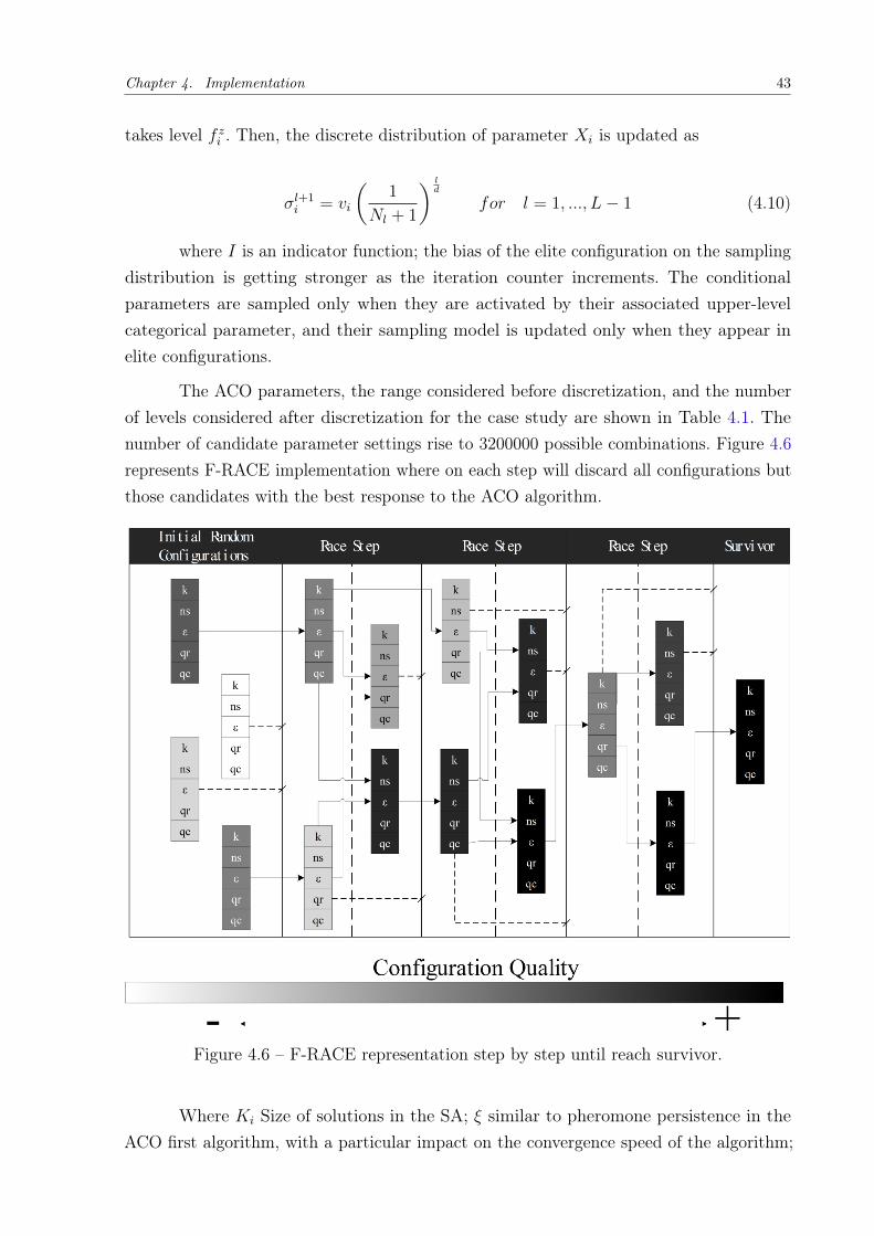
Chapter 4. Implementation 43
takes level f zi . Then, the discrete distribution of parameter Xi is updated as
σl+1i = vi
(1
Nl + 1
) ld
for l = 1, ..., L− 1 (4.10)
where I is an indicator function; the bias of the elite configuration on the samplingdistribution is getting stronger as the iteration counter increments. The conditionalparameters are sampled only when they are activated by their associated upper-levelcategorical parameter, and their sampling model is updated only when they appear inelite configurations.
The ACO parameters, the range considered before discretization, and the numberof levels considered after discretization for the case study are shown in Table 4.1. Thenumber of candidate parameter settings rise to 3200000 possible combinations. Figure 4.6represents F-RACE implementation where on each step will discard all configurations butthose candidates with the best response to the ACO algorithm.
Figure 4.6 – F-RACE representation step by step until reach survivor.
Where Ki Size of solutions in the SA; ξ similar to pheromone persistence in theACO first algorithm, with a particular impact on the convergence speed of the algorithm;

Chapter 4. Implementation 44
Table 4.1 – The range of ACO parameters considered.
Parameters Range No. of levelsKi [ 10 - 800 ]
20ξ [ 0.1 - 1.2 ]ns [ 1 - 80]qR [ 0.0001 - 0.1 ]qC
ns Number of new solutions (ants); q Parameter to increase elitism of the algorithm (qrContinuous qc Categorical).
4.8 High-Quality Initial Solution
Ordinarily, SA initiates by a random sampling of the feasible space gives byconstraints 3.9 and 3.10. Formally, ACO uses a normal random generation for the initialsolution, limiting such procedure to constraints feasible values improve the quality of theSA (GOTTLIEB et al., 2003; BLUM, 2005).
Normally, improving initial solution leads to better solutions quality (ZHANG etal., 2011). For the coordination of DOCRs as nonlinear programming (NLP) problem,relaxation introduced by (URDANETA et al., 1988) gives an opportunity to create a newhigh-quality SA based on it. Creating k PS vectors part of the ACO, remembering k isthe size of initial population for de ACO algorithm and consequently, the size of ACO.k will be, also, the number of linear programming (LP) problems to solve, and the TDSobtain will replace TDS random generated as shown in Fig. 4.7.
Figure 4.7 – Flowchart including high-quality initial solution built
Notice, the possibility of finding unfeasible LP problems derivate that TDS initialrandom values must stay in memory until LP Process is completed because a PS vector

Chapter 4. Implementation 45
could create a non-feasible LP problem. It is expected a minimum of unfeasible LP problemsfrom the last step, required for diversity in the ACO building solution process.
In general, the flowchart on Fig. 4.7, stand on the next premises, starts with theselection of the system (3 and 8 Bus for this work), loading data for such system. Randomgeneration for relay PS/TDS to build the ACO. A decision box plants if is required tobuild an improved initial solution, if Yes is chosen, trigger a LP problem solver for eachPS initial solution vector, if solution found is feasible it re-writes TDS values randomgenerated. At this point, also if the choice NO is selected, the ACO is passed to the ACOMulti-variable algorithm to solve the entire Coordination Problem.
4.9 Hybrid Technique ACO-LP
Many hybrid methods are an important mechanism in integer programming, asthey combine the best features of different methods in a complementary manner. Withan effort to reduce computation times and relax this non-linear problem next framework(see Fig. 4.8) is presented with the idea to solve the categorical variable using a classicalapproach of ACO Algorithm, as showed in Section 4.4.1, and solving continuous variablethrough a relaxation of the problem using linear programming.
The flowchart on Fig. 4.8 follows with the selection of the system, loading suchdata. Random generation for relay PS/TDS (and tZ2 according case of study) to buildthe LP problem to solve the relaxed problem, and re-writing TDS and tZ2 to only feasibleconfigurations. Initiating ACO predefined process based on ranking and quality functionto build new PSs is needed. At this point, stop criteria is evaluated to is passed or to theACO algorithm or to the end with the optimal solution.
4.10 Solution Space Estimate - Linear Relaxation
As Noghabi et al. (2009) is valid to count the number of possible combinations ofPS (Only for discrete characteristics) for estimation. Once all available PS combinationsare estimated, the optimal solution to the problem may be found. Because, for eachcombination of PS, the optimal TDS can be calculated using LP. Thus, the estimation ofthe solution space (LPmax) based on LP can be calculated by
LPmax =n∏i
NPSi (4.11)
where NPSi is the number of PS adjustments available for n relays.
For a small number of relays is possible to do an exhaustive analysis to compareheuristics performance. Getting to the global optimal solution of the problem.

Chapter 4. Implementation 46
Figure 4.8 – Flowchart for Hybrid Scheme ACO-LP

47
5 Testing Systems
The proposed methods are applied to five transmission systems (3, 6, 8, 9, and15 Bus accordingly) IEEE bus systems. Numerical results designate the advantages andvalidation of this work.
5.1 System I: Three Bus Network
In the System I, the proposed algorithm is applied to the three-bus system presentedin Fig. 5.1. It has three buses, three lines, three generators and six DOCRs. Detailed dataof this system are presented by author Amraee (2012). The coordination is done for three-phase faults in the midpoint of each line. Moreover, there are six selectivity constraints forthe steady and transient configuration of the system, totalizing 12 constraints. Steady andtransient configuration where normally considered for analog relays within former powersystems. The PS is considered as discrete, and it varies from 1.5 to 5.0 A, in uniformsteps of 0.5 A. Thus, this system has discrete PS and continuous TDS. The maximum andminimum TDS are 1.1 and 0.1, respectively. The adopted value of CTI is 0.2 s.
Figure 5.1 – Single-line diagram of the three-bus system.
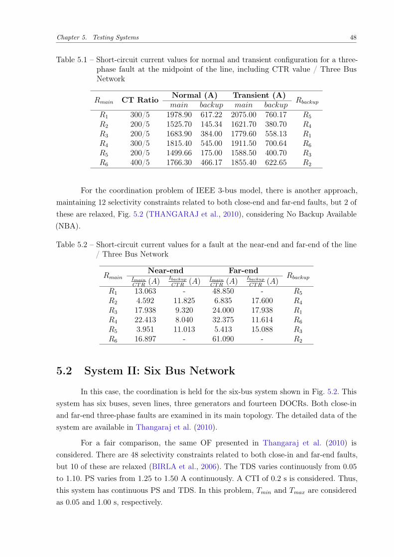
Chapter 5. Testing Systems 48
Table 5.1 – Short-circuit current values for normal and transient configuration for a three-phase fault at the midpoint of the line, including CTR value / Three BusNetwork
Rmain CT Ratio Normal (A) Transient (A)Rbackupmain backup main backup
R1 300/5 1978.90 617.22 2075.00 760.17 R5
R2 200/5 1525.70 145.34 1621.70 380.70 R4
R3 200/5 1683.90 384.00 1779.60 558.13 R1
R4 300/5 1815.40 545.00 1911.50 700.64 R6
R5 200/5 1499.66 175.00 1588.50 400.70 R3
R6 400/5 1766.30 466.17 1855.40 622.65 R2
For the coordination problem of IEEE 3-bus model, there is another approach,maintaining 12 selectivity constraints related to both close-end and far-end faults, but 2 ofthese are relaxed, Fig. 5.2 (THANGARAJ et al., 2010), considering No Backup Available(NBA).
Table 5.2 – Short-circuit current values for a fault at the near-end and far-end of the line/ Three Bus Network
RmainNear-end Far-end
RbackupImain
CTR(A)
IbackupCTR
(A) Imain
CTR(A)
IbackupCTR
(A)R1 13.063 - 48.850 - R5
R2 4.592 11.825 6.835 17.600 R4
R3 17.938 9.320 24.000 17.938 R1
R4 22.413 8.040 32.375 11.614 R6
R5 3.951 11.013 5.413 15.088 R3
R6 16.897 - 61.090 - R2
5.2 System II: Six Bus Network
In this case, the coordination is held for the six-bus system shown in Fig. 5.2. Thissystem has six buses, seven lines, three generators and fourteen DOCRs. Both close-inand far-end three-phase faults are examined in its main topology. The detailed data of thesystem are available in Thangaraj et al. (2010).
For a fair comparison, the same OF presented in Thangaraj et al. (2010) isconsidered. There are 48 selectivity constraints related to both close-in and far-end faults,but 10 of these are relaxed (BIRLA et al., 2006). The TDS varies continuously from 0.05
to 1.10. PS varies from 1.25 to 1.50 A continuously. A CTI of 0.2 s is considered. Thus,this system has continuous PS and TDS. In this problem, Tmin and Tmax are consideredas 0.05 and 1.00 s, respectively.
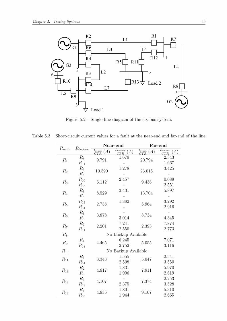
Chapter 5. Testing Systems 49
Figure 5.2 – Single-line diagram of the six-bus system.
Table 5.3 – Short-circuit current values for a fault at the near-end and far-end of the line
Rmain RbackupNear-end Far-end
Imain
CTR(A)
IbackupCTR
(A) Imain
CTR(A)
IbackupCTR
(A)
R1R8 9.791 1.679 20.794 2.343R11 - 1.667
R2R3 10.590 1.278 23.015 3.425R5 - -
R3R10 6.112 2.457 9.438 0.089R13 - 2.551
R4R1 8.529 3.431 13.704 5.897R5 - -
R5R12 2.738 1.882 5.964 3.292R14 - 2.916
R6R1 3.878 - 8.734 -R3 3.014 4.345
R7R2 2.201 7.241 2.393 7.874R11 2.550 2.773
R8 No Backup Available
R9R4 4.465 6.245 5.055 7.071R13 2.752 3.116
R10 No Backup Available
R11R6 3.343 1.555 5.047 2.541R14 2.508 3.550
R12R2 4.917 1.831 7.911 5.970R8 1.906 2.619
R13R6 4.107 - 7.374 2.253R12 2.375 3.528
R14R4 4.935 1.801 9.107 5.310R10 1.944 2.665

Chapter 5. Testing Systems 50
5.3 System III: Eight Bus Network
The next system is shown in Fig. 5.3. This network has eight buses, seven lines,two generators and fourteen DOCRs. EG is an external grid modeled with a short-circuitcapacity of 400 MVA. Detailed data of this system are presented in Amraee (2012). Thereare 20 selectivity constraints related to near-end three-phase faults. The available PS are0.5, 0.6, 0.8, 1.0, 1.5, 2.0 and 2.5 A. The TDS is considered as continuous and it variesfrom 0.1 to 1.1. A CTI of 0.3 s is considered according to previous authors.
Figure 5.3 – Single-line diagram of the eight-bus system.

Chapter 5. Testing Systems 51
Table 5.4 – Short-circuit current values for normal and transient configuration for a faultat the midpoint of the line, including CTR value
Rmain CT Ratio Imain (A) Ibackup (A) Rbackup
R1 1200/5 3232 996 R6
R2 1200/5 5924 3556 R1
R7
R3 800/5 3556 2244 R2
R4 1200/5 3783 2401 R3
R5 1200/5 2401 1197 R4
R6 1200/5 6109 3232 R14
R5
R7 800/5 5223 1890 R13
R5
R8 1200/5 6093 2991 R9
R7
R9 800/5 2484 1165 R10
R10 1200/5 3883 2484 R11
R11 1200/5 3707 2344 R12
R12 1200/5 5899 3707 R14
R13
R13 1200/5 2991 987 R8
R14 800/5 5199 1874 R1
R9
5.4 System IV: Nine Bus Network
The system IV presented, shown in Fig. 5.4. This network has nine buses, twelvelines, one generator and twenty-four DOCRs. Detailed data of the system are availablein Bedekar and Bhide (2011b). All current transformer rate (CTR) are considered as500/1. In this case, the minimum and maximum value of PS are computed with practicalconsiderations, as shown in (5.1) Bedekar and Bhide (2011b). The minimum and maximumvalues of TDS are 0.025 and 1.2, respectively. Both TDS and PS are considered ascontinuous variables. There are 44 selectivity constraints in this problem. A CTI of 0.2 sis adopted according to previous authors. The minimum operational time is 0.2 s. 1.25 isthe load factor apply in previous works.
1.25 · I iloadCTRi
≤ PSi ≤2 · Iccimin3 · CTRi
(5.1)
where I iload is the maximum load current through Ri, Iccimin is the minimum fault currentsensed by Ri.

Chapter 5. Testing Systems 52
Figure 5.4 – Single-line diagram of the nine-bus system.

Chapter 5. Testing Systems 53
Table 5.5 – Short-circuit current values for normal and transient configuration for a faultat the midpoint of the line
Rmain Imain (A) Iload (A) Ibackup (A) Rbackup
R1 4863.60 121.74 1293.90 R17
1168.30 R15
R2 1634.40 212.74 1044.20 R4
R3 2811.40 21.74 1361.60 R1
R4 2610.50 21.74 1226.00 R6
R5 1778.00 78.26 1124.40 R3
R6 4378.50 78.26 1345.50 R23
711.20 R8
R7 4378.50 78.26 1345.50 R23
711.20 R5
R8 1778.00 78.26 1124.40 R10
R9 2610.50 21.74 1226.00 R7
R10 2811.40 21.74 787.20 R12
R11 1634.40 121.74 1044.20 R9
R12 2811.40 121.74 1293.90 R21
1168.30 R14
R13 3684.50 30.44 1293.90 R21
653.60 R11
R14 4172.50 30.44 1264.10 R19
1031.70 R16
R15 4172.50 30.44 1264.10 R19
1031.70 R13
R16 3684.50 30.44 1293.90 R17
653.60 R2
R17 7611.20 441.30 1432.30 R24
R18 2271.70 441.30 1168.30 R15
653.60 R2
R19 7435.80 410.87 1432.30 R24
R20 2624.20 410.87 1031.70 R13
1031.70 R16
R21 7611.20 441.30 1432.30 R24
R22 2271.70 441.30 653.60 R11
1168.30 R14
R23 7914.70 506.52 1953.70 R22
R24 1665.50 506.52 711.20 R8
711.20 R5
5.5 System V: Fifteen Bus Network
The last case relates to the system presented in Fig. 5.5. This network has 15 buses,21 lines, 6 generators and 42 DOCRs. EG is an external grid molded with a short-circuitcapacity of 200 MVA. Complete data of this system are presented in Amraee (2012).This problem has 82 selectivity constraints associated to near-end three-phase faults.

Chapter 5. Testing Systems 54
The minimum and maximum values of PS are 0.5 and 2.5 A, in uniform steps of 0.5 A,respectively. The TDS are continuous variables that vary from 0.1 to 1.1. It is considereda CTI of 0.2 s.
Figure 5.5 – Single-line diagram of the fifteen-bus system.

Chapter 5. Testing Systems 55
Table 5.6 – Short-circuit current values for normal and transient configuration for a faultat the midpoint of the line
Rmain CTRatio
Imain(A)
Ibackup(A)
Rbackup Rmain CTRatio
Imain(A)
Ibackup(A)
Rbackup
R1 800/5 3621 853 R6 R20 1600/5 7662 1808 R30
R2 1200/5 4597 922 R4
R21 1600/5 8384 1326R19
R16 R17
R3 800/5 3984 1424 R1 R30
R16 R22 400/5 1950 642 R23
R4 1200/5 4382 1477R7 R34
R12 R23 1200/5 4910 979 R13
R20 R11
R5 800/5 3319 1397 R2 R24 600/5 2296 753 R21
R6 600/5 2647 1233 R10 R34
R8 R25 600/5 2289 903 R15
R7 600/5 2497 1111 R5 R18
R10 R26 600/5 2300 905 R28
R8 1200/5 4695 1548R3 R36
R12 R27 600/5 2011 1039 R25
R20 R36
R9 600/5 2943 1009 R5 R28 600/5 2525 1192 R29
R8 R32
R10 800/5 3568 1100 R14
R29 1600/5 8346 1828R19
R11 1200/5 4342 1475R7 R17
R3 R22
R20 R30 400/5 1736 681 R27
R12 1200/5 4195 1463 R13 R32
R24 R31 600/5 2867 809 R29
R13 800/5 3402 1503 R9 R27
R14 1200/5 4606 1175 R11 R32 600/5 2069 697 R33
R24 R42
R15 1200/5 4712 969 R1 R33 600/5 2305 1162 R23
R4 R21
R16 600/5 2225 743 R18 R34 400/5 1715 970 R31
R26 R42
R17 400/5 1875 599 R15 R35 600/5 2095 910 R25
R26 R28
R18 1600/5 8426 1320R19 R36 800/5 3283 1109 R38
R22 R37 800/5 3301 1434 R35
R30 R38 400/5 1403 882 R40
R19 800/5 3998 1372R7 R39 400/5 1434 896 R37
R3 R40 800/5 3140 1403 R41
R12 R41 400/5 1971 745 R33
R20 1600/5 7662 1808 R17 R31
R22 R42 800/5 3295 907 R39
56
6 Results and Discussions
This chapter refers to the results and discussions resulting from simulating themethodology proposed for the relay coordination in meshed transmission systems.
The method was validated using five transmission systems in the specializedliterature, the 3, 6, 8, 9 and 15 standard systems, the results are compared with thosereported in the literature under same conditions, when there is no available data for themodel propose, validation goes by feasible evaluation for the specific problem.
Simulations were performed on an Intel ®-based processor Core™i5-2430M 2.4GHzwith 8GB of RAM DDR3 running operating system Windows 10 64 bits and for parallelcomputing testing an Intel ®-based processor Xeon™E5-2430v2 2.2 Ghz with 24GB ofRAM DDR3 running operating system Windows 7 64 bits. Implemented in Matlab 2016a.
The objective function verifies the minimization of the time for the primary relays(DOCR and/or Distance), also evaluating how feasible is the solution and computing it asunfitness, getting a quality function to guide the algorithm.
6.1 System I: Three Bus Network
For System I, there are two possible configurations, first, Mid-Point Faults whichis only able to perform DOCRs Coordination, and Near-end and Far-end Faults to applya simple DOCRs Coordination and also a combined scheme with Distance Relays. ForMid-Point Fault besides comparing with other meta-heuristic techniques in the literatureis also an additional validation using an exhaustive search to get a deterministic solutionusing LP.
6.1.1 DOCRs Only
Mid-Point Fault for 3-bus System
The algorithm runs a hundred times with five different configurations evaluatingOF value (See Tab. 6.1) and Execution time (See Tab. 6.2). Those configurations areOptimized ACOMV for 5000 and 1000 Iterations, an additional 1000 iterations using aninitial high-quality solution (IHQS), ACOMV with not optimized parameters, and a Hybridconfiguration based on ACO − LP .
The best solution found occurs under ACO − LP (Hybrid) scenario and is shownon Tab. 6.4. Tripping times for coordinated configuration may be checked on Table 6.3 forbest implemented technique.
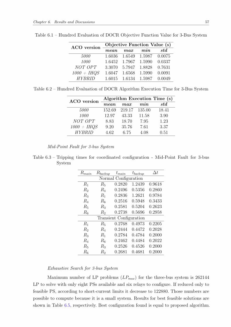
Chapter 6. Results and Discussions 57
Table 6.1 – Hundred Evaluation of DOCR Objective Function Value for 3-Bus System
ACO version Objective Function Value (s)mean max min std
5000 1.6036 1.6549 1.5987 0.00751000 1.6452 1.7967 1.5990 0.0337
NOT OPT 3.3070 5.7947 1.8828 0.76311000 + IHQS 1.6047 1.6568 1.5990 0.0091HYBRID 1.6015 1.6134 1.5987 0.0049
Table 6.2 – Hundred Evaluation of DOCR Algorithm Execution Time for 3-Bus System
ACO version Algorithm Execution Time (s)mean max min std
5000 152.69 219.17 135.00 18.411000 12.97 43.33 11.58 3.90
NOT OPT 8.83 18.70 7.95 1.231000 + IHQS 9.20 35.76 7.61 3.37HYBRID 4.62 6.75 4.08 0.51
Mid-Point Fault for 3-bus System
Table 6.3 – Tripping times for coordinated configuration - Mid-Point Fault for 3-busSystem
Rmain Rbackup tmain tbackup ∆tNormal Configuration
R1 R5 0.2820 1.2439 0.9618R2 R4 0.2496 0.5356 0.2860R3 R1 0.2836 1.2621 0.9784R4 R6 0.2516 0.5948 0.3433R5 R3 0.2581 0.5204 0.2623R6 R2 0.2738 0.5696 0.2958
Transient ConfigurationR1 R5 0.2768 0.4973 0.2205R2 R4 0.2444 0.4472 0.2028R3 R1 0.2784 0.4784 0.2000R4 R6 0.2462 0.4484 0.2022R5 R3 0.2526 0.4526 0.2000R6 R2 0.2681 0.4681 0.2000
Exhaustive Search for 3-bus System
Maximum number of LP problems (LPmax) for the three-bus system is 262144
LP to solve with only eight PSs available and six relays to configure. If reduced only tofeasible PS, according to short-current limits it decrease to 122880. Those numbers arepossible to compute because it is a small system. Results for best feasible solutions areshown in Table 6.5, respectively. Best configuration found is equal to proposed algorithm.
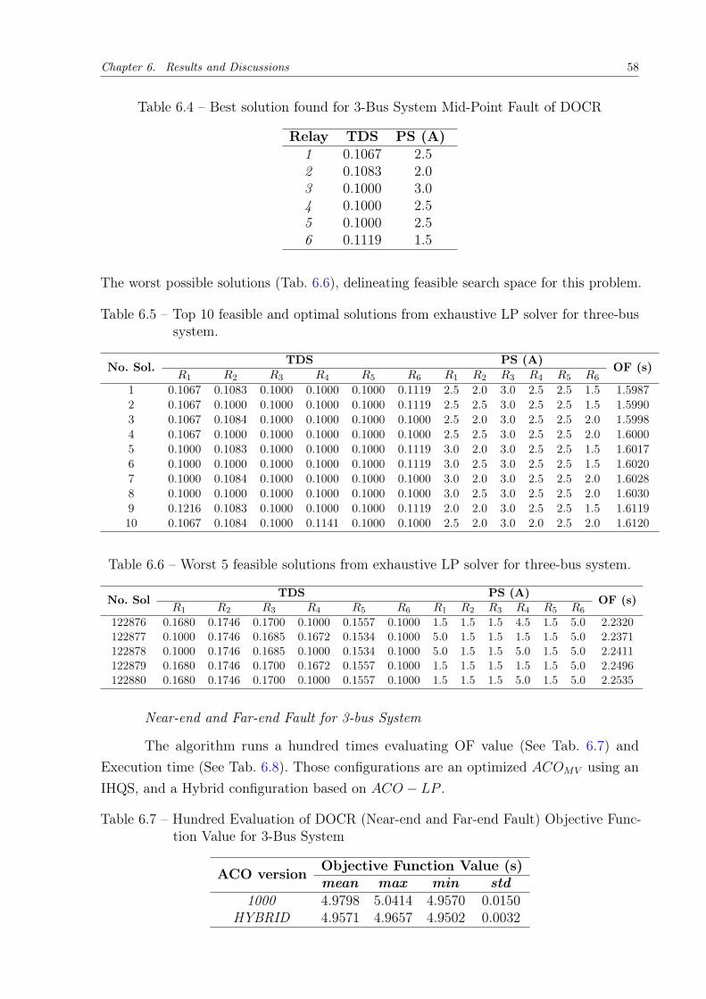
Chapter 6. Results and Discussions 58
Table 6.4 – Best solution found for 3-Bus System Mid-Point Fault of DOCR
Relay TDS PS (A)1 0.1067 2.52 0.1083 2.03 0.1000 3.04 0.1000 2.55 0.1000 2.56 0.1119 1.5
The worst possible solutions (Tab. 6.6), delineating feasible search space for this problem.
Table 6.5 – Top 10 feasible and optimal solutions from exhaustive LP solver for three-bussystem.
No. Sol. TDS PS (A) OF (s)R1 R2 R3 R4 R5 R6 R1 R2 R3 R4 R5 R6
1 0.1067 0.1083 0.1000 0.1000 0.1000 0.1119 2.5 2.0 3.0 2.5 2.5 1.5 1.59872 0.1067 0.1000 0.1000 0.1000 0.1000 0.1119 2.5 2.5 3.0 2.5 2.5 1.5 1.59903 0.1067 0.1084 0.1000 0.1000 0.1000 0.1000 2.5 2.0 3.0 2.5 2.5 2.0 1.59984 0.1067 0.1000 0.1000 0.1000 0.1000 0.1000 2.5 2.5 3.0 2.5 2.5 2.0 1.60005 0.1000 0.1083 0.1000 0.1000 0.1000 0.1119 3.0 2.0 3.0 2.5 2.5 1.5 1.60176 0.1000 0.1000 0.1000 0.1000 0.1000 0.1119 3.0 2.5 3.0 2.5 2.5 1.5 1.60207 0.1000 0.1084 0.1000 0.1000 0.1000 0.1000 3.0 2.0 3.0 2.5 2.5 2.0 1.60288 0.1000 0.1000 0.1000 0.1000 0.1000 0.1000 3.0 2.5 3.0 2.5 2.5 2.0 1.60309 0.1216 0.1083 0.1000 0.1000 0.1000 0.1119 2.0 2.0 3.0 2.5 2.5 1.5 1.611910 0.1067 0.1084 0.1000 0.1141 0.1000 0.1000 2.5 2.0 3.0 2.0 2.5 2.0 1.6120
Table 6.6 – Worst 5 feasible solutions from exhaustive LP solver for three-bus system.
No. Sol TDS PS (A) OF (s)R1 R2 R3 R4 R5 R6 R1 R2 R3 R4 R5 R6
122876 0.1680 0.1746 0.1700 0.1000 0.1557 0.1000 1.5 1.5 1.5 4.5 1.5 5.0 2.2320122877 0.1000 0.1746 0.1685 0.1672 0.1534 0.1000 5.0 1.5 1.5 1.5 1.5 5.0 2.2371122878 0.1000 0.1746 0.1685 0.1000 0.1534 0.1000 5.0 1.5 1.5 5.0 1.5 5.0 2.2411122879 0.1680 0.1746 0.1700 0.1672 0.1557 0.1000 1.5 1.5 1.5 1.5 1.5 5.0 2.2496122880 0.1680 0.1746 0.1700 0.1000 0.1557 0.1000 1.5 1.5 1.5 5.0 1.5 5.0 2.2535
Near-end and Far-end Fault for 3-bus System
The algorithm runs a hundred times evaluating OF value (See Tab. 6.7) andExecution time (See Tab. 6.8). Those configurations are an optimized ACOMV using anIHQS, and a Hybrid configuration based on ACO − LP .
Table 6.7 – Hundred Evaluation of DOCR (Near-end and Far-end Fault) Objective Func-tion Value for 3-Bus System
ACO version Objective Function Value (s)mean max min std
1000 4.9798 5.0414 4.9570 0.0150HYBRID 4.9571 4.9657 4.9502 0.0032

Chapter 6. Results and Discussions 59
Table 6.8 – Hundred Evaluation of DOCR (Near-end and Far-end Fault) Algorithm Exe-cution Time for 3-Bus System
ACO version Algorithm Execution Time (s)mean max min std
1000 121.10 175.36 115.57 6.02HYBRID 15.45 19.74 13.77 1.57
The best solution found is shown on Tab. 6.11 for both parameters, TDS and PS.Tripping times for coordinated configuration may be checked on Table 6.9 for best priorimplemented technique and Table 6.10 for the hybrid algorithm.
Table 6.9 – Tripping times for coordinated configuration - Near-end and Far-end Fault for3-bus System
Rmain Rbackup tmain tbackup ∆tNear-end
R1 R5 0.1457 0.3457 0.2000R2 R4 0.5911 0.7928 0.2016R3 R1 0.7170 NBA NBAR4 R6 0.4916 NBA NBAR5 R3 0.6607 0.9708 0.3101R6 R2 0.1310 0.3387 0.2077
Far-endR1 R5 0.0920 0.3010 0.2090R2 R4 0.4507 0.6507 0.2000R3 R1 0.6418 NBA NBAR4 R6 0.4319 NBA NBAR5 R3 0.5170 0.7170 0.2000R6 R2 0.0865 0.2865 0.2000

Chapter 6. Results and Discussions 60
Table 6.10 – Tripping times for coordinated (Hybrid) configuration - Near-end and Far-endFault for 3-bus System
Rmain Rbackup tmain tbackup ∆tNear-end
R1 R5 0.1457 0.3457 0.2000R2 R4 0.5909 0.7956 0.2048R3 R1 0.7170 NBA NBAR4 R6 0.4894 NBA NBAR5 R3 0.6606 0.9795 0.3189R6 R2 0.1309 0.3387 0.2077
Far-endR1 R5 0.0920 0.3011 0.2090R2 R4 0.4506 0.6505 0.2000R3 R1 0.6390 NBA NBAR4 R6 0.4306 NBA NBAR5 R3 0.5170 0.7170 0.2000R6 R2 0.0865 0.2865 0.2000
Table 6.11 – Best solution found for 3-Bus System (Near-end and Far-end Fault) of DOCR
Relay TDS PS (A)1 0.0500 1.2512 0.1110 1.25283 0.2613 1.48964 0.1945 1.49355 0.1098 1.25066 0.0500 1.2501
6.1.2 Distance and DOCRs (Near-end and Far-end Fault)
The algorithm runs a hundred times evaluating OF value (See Tab. 6.12) andExecution time (See Tab. 6.13). Those configurations are an optimized ACOMV using anIHQS, and a Hybrid configuration based on ACO − LP .
Table 6.12 – Hundred Evaluation of Distance-DOCR Objective Function Value for 3-BusSystem
ACO version Objective Function Value (s)mean max min std
1000 13.0659 13.1952 12.9951 0.0772HYBRID 11.5003 11.6378 11.3129 0.0699
The best solution found is shown on Tab. 6.16 for three parameters, TDS,PS, andtZ2. Tripping times for coordinated configuration may be checked on Table 6.14 for bestprior implemented technique and Table 6.15 for the hybrid algorithm.
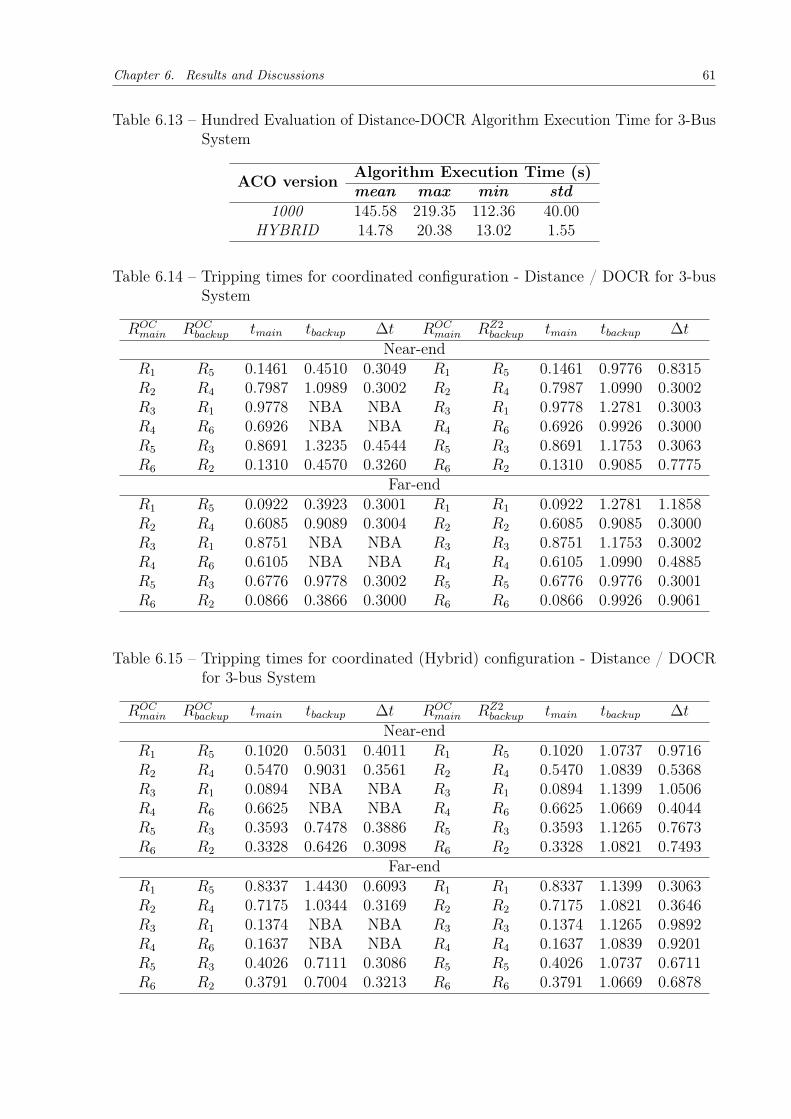
Chapter 6. Results and Discussions 61
Table 6.13 – Hundred Evaluation of Distance-DOCR Algorithm Execution Time for 3-BusSystem
ACO version Algorithm Execution Time (s)mean max min std
1000 145.58 219.35 112.36 40.00HYBRID 14.78 20.38 13.02 1.55
Table 6.14 – Tripping times for coordinated configuration - Distance / DOCR for 3-busSystem
ROCmain ROC
backup tmain tbackup ∆t ROCmain RZ2
backup tmain tbackup ∆t
Near-endR1 R5 0.1461 0.4510 0.3049 R1 R5 0.1461 0.9776 0.8315R2 R4 0.7987 1.0989 0.3002 R2 R4 0.7987 1.0990 0.3002R3 R1 0.9778 NBA NBA R3 R1 0.9778 1.2781 0.3003R4 R6 0.6926 NBA NBA R4 R6 0.6926 0.9926 0.3000R5 R3 0.8691 1.3235 0.4544 R5 R3 0.8691 1.1753 0.3063R6 R2 0.1310 0.4570 0.3260 R6 R2 0.1310 0.9085 0.7775
Far-endR1 R5 0.0922 0.3923 0.3001 R1 R1 0.0922 1.2781 1.1858R2 R4 0.6085 0.9089 0.3004 R2 R2 0.6085 0.9085 0.3000R3 R1 0.8751 NBA NBA R3 R3 0.8751 1.1753 0.3002R4 R6 0.6105 NBA NBA R4 R4 0.6105 1.0990 0.4885R5 R3 0.6776 0.9778 0.3002 R5 R5 0.6776 0.9776 0.3001R6 R2 0.0866 0.3866 0.3000 R6 R6 0.0866 0.9926 0.9061
Table 6.15 – Tripping times for coordinated (Hybrid) configuration - Distance / DOCRfor 3-bus System
ROCmain ROC
backup tmain tbackup ∆t ROCmain RZ2
backup tmain tbackup ∆t
Near-endR1 R5 0.1020 0.5031 0.4011 R1 R5 0.1020 1.0737 0.9716R2 R4 0.5470 0.9031 0.3561 R2 R4 0.5470 1.0839 0.5368R3 R1 0.0894 NBA NBA R3 R1 0.0894 1.1399 1.0506R4 R6 0.6625 NBA NBA R4 R6 0.6625 1.0669 0.4044R5 R3 0.3593 0.7478 0.3886 R5 R3 0.3593 1.1265 0.7673R6 R2 0.3328 0.6426 0.3098 R6 R2 0.3328 1.0821 0.7493
Far-endR1 R5 0.8337 1.4430 0.6093 R1 R1 0.8337 1.1399 0.3063R2 R4 0.7175 1.0344 0.3169 R2 R2 0.7175 1.0821 0.3646R3 R1 0.1374 NBA NBA R3 R3 0.1374 1.1265 0.9892R4 R6 0.1637 NBA NBA R4 R4 0.1637 1.0839 0.9201R5 R3 0.4026 0.7111 0.3086 R5 R5 0.4026 1.0737 0.6711R6 R2 0.3791 0.7004 0.3213 R6 R6 0.3791 1.0669 0.6878

Chapter 6. Results and Discussions 62
Table 6.16 – Best solution found for 3-Bus System (Near-end and Far-end Fault) ofDistance-DOCR
Relay TDS PS (A) tZ2 (s)1 0.0541 1.3605 1.13992 0.1348 1.2536 1.08203 0.1463 1.4978 1.12654 0.1515 1.4722 1.08385 0.1406 1.2517 1.07366 0.0500 1.4085 1.0669
6.1.3 ACO Parameters Optimization with F-RACE
Table 6.17 contains survivors from the racing optimization algorithm for System I,based on a quality function to get better configuration on each iteration. Time neededto this algorithm seizes that answer was over 3 hours for a single 4-core desktop and 36minutes for a 24-core cluster.
Table 6.17 – Survivors of the F-RACE Algorithm for 3-Bus System
k ξ nS qR qC210 0.815 55 0.0201 0.0201 1.601250 1.035 58 0.0151 0.0650 1.6030130 0.980 52 0.0201 0.0401 1.6044130 1.145 73 0.0201 0.0301 1.6049130 1.035 43 0.0151 0.0600 1.605850 1.200 43 0.0251 0.0900 1.6069170 0.815 55 0.0301 0.0451 1.6073210 0.815 58 0.0301 0.0451 1.6081210 0.760 58 0.0301 0.0201 1.6093130 1.090 49 0.0151 0.0850 1.6093250 0.815 46 0.0251 0.0251 1.6094170 0.870 52 0.0201 0.0501 1.6101130 0.815 73 0.0301 0.0600 1.6116170 0.870 52 0.0251 0.0650 1.6121170 1.090 67 0.0251 0.0401 1.6122170 1.090 67 0.0301 0.0600 1.6123130 1.035 43 0.0201 0.1000 1.6127130 0.980 49 0.0251 0.0900 1.6127250 0.980 43 0.0201 0.0700 1.6137210 0.925 37 0.0351 0.0650 1.6182170 0.650 34 0.0301 0.0251 1.620490 1.035 49 0.0151 0.0750 1.6209250 0.760 58 0.0301 0.0650 1.6214170 0.705 73 0.0251 0.0700 1.624350 0.980 40 0.0201 0.1000 1.6271
Within that result is measure statistical data (see Tab. 6.18) to select the parameters

Chapter 6. Results and Discussions 63
according to the race survivors, this data is also important to define which parameter hasmore influence on the algorithm performance.
Table 6.18 – Comparing for Survivors of the F-RACE Algorithm for 3-Bus System
k ξ nS qR qCmean 157 0.932 53 0.024 0.058max 250 1.200 73 0.035 0.100min 50 0.650 34 0.015 0.020std 57 0.143 11 0.006 0.024
Influence 13.18% 31.38% 23.37% 20.16% 11.90%
6.1.4 Validation
Fig. 6.1 represent three OF, according to ACO optimized, ACO optimized withthe introduction of an initial High-Quality Solution and an ACO without parametersoptimization. Except for ACO NOT OPT, both get optimal answers based on Table 6.1,in this occasion ACO + IHQS, obtain the best optimal solution as may be confirmed byTable 6.5, but is also evident how fast is the convergence of this method which for ansmall size system is optimal may not be guaranteed for larger systems. It is important tonotice how restart mechanism acts over OF (around iteration No 500) fighting stagnationand improving value closer to the optimal.
0 100 200 300 400 500 600 700 800 900 1000Iteration
0
1
2
3
4
5
6
7
8
9
OF
Val
ue
ACOACO + IHQSACO NOT OPTRESTART
Figure 6.1 – OF Value for Single ACO, ACO NOT OPT, and ACO + IHQS for a 3-BusSystem.
OF value from ACO-LP for a 3-Bus System shows in Fig. 6.2 fast convergence infew iterations into optimal value.

Chapter 6. Results and Discussions 64
1 2 3 4 5 6 7 8 9 10Iteration
1.5
2
2.5
3
3.5
4
OF
Val
ue -
Mid
poin
t
4.94
4.96
4.98
5
5.02
5.04
5.06
5.08
5.1
5.12
OF
Val
ue -
NE
/FE
MidpointNE/FE
Figure 6.2 – OF value Coordination with ACO-LP for a 3-Bus System
The output from Distance-DOCR Coordination with ACO-LP for a 3-Bus System(Fig. 6.3), shows an inverse convergence in the OF value until configuration enters into thefeasible region.
1 2 3 4 5 6 7 8 9 10Iteration
7.5
8
8.5
9
9.5
10
10.5
11
11.5
12
0
50
100
150
200
250
300
350OF ValueUnfitness Value
Figure 6.3 – Distance-DOCR Coordination with ACO-LP for a 3-Bus System
This work, for System I, obtained optimal for this problem (OF = 1.5987) in4.6154 s for ACO − LP and 12.5591 s for ACO −MV , better than PSO (MANSOUR etal., 2007), Biogeography Based Optimization (BBO) (ALBASRI et al., 2015), and SeekerOptimization Algorithm (SOA) (AMRAEE, 2012), and same as BBO-LP (ALBASRI etal., 2015) and GACB-LP (KIDA, 2016) but slower than both (Table 6.19).

Chapter 6. Results and Discussions 65
Table 6.19 – Results Comparison for 3-Bus System Mid-Point Fault DOCR
Tech Autor Exe Time (s) OF - Time (s)PSO (MANSOUR et al., 2007) 0.5129 1.9258BBO (ALBASRI et al., 2015) 16.2300 1.6837SOA (AMRAEE, 2012) 10.4500 1.5990
BBO-LP (ALBASRI et al., 2015) 2.9900 1.5987GACB-LP (KIDA, 2016) 0.2047 1.5987ACO-MV This Work 12.5591 1.5987ACO-LP This Work 4.6154 1.5987
For Near-end and Far-end Fault solution found is close to those from RhetoricalStructure Theory (RST) (DEEP et al., 2006) and Modified Differential Evolution v5(MDE5) (THANGARAJ et al., 2010) but with a number of function evaluation (NFE)consistently better than best answer available for both techniques applied.
Table 6.20 – Results Comparison for 3-Bus System (Near-end and Far-end Fault) DOCR
Tech Autor NFE OF - Time (s)ACO-MV This Work 1000 4.9570ACO-LP This Work 10 4.9502
RST (DEEP et al., 2006) N/A 4.8354MDE5 (THANGARAJ et al., 2010) 69270 4.7806
Distance-DOCR coordination based on Near-end and Far-end Fault was not possibleto validate with literature, in order to build this model must be assumed fault locations todistinguish Primary-Backup for this mixed scheme. Data from Table 6.12 shows violationof the upper limit according to Table 3.5 where maximum is mark by 0.6 s, but as showsin Perez and Urdaneta (2001) those limits are normally design by dealers under uniquedistance coordination.
6.2 System II: Six Bus Network
For System II, there is only one possible configuration Near-end and Far-end Faultsto apply a simple DOCRs Coordination and also a combined scheme with Distance Relays.
For this system comparing with other meta-heuristic techniques in the literature isalso offered.
6.2.1 DOCRs Only
The algorithm runs a hundred times with four different configurations evaluatingOF value (See Tab. 6.21) and Execution time (See Tab. 6.22). Those configurations areOptimized ACOMV for 2000 Iterations, an additional 2000 iterations using an IHQS, also

Chapter 6. Results and Discussions 66
is presented an ACOMV with not optimized parameters, and a Hybrid configuration basedon ACO − LP .
Table 6.21 – Hundred Evaluation of DOCR (Near-end and Far-end Fault) Value for 6-BusSystem
ACO version OFmean max min std
2000 10.4429 12.7379 10.1584 0.3247NOT OPT 14.9275 15.2051 14.2624 0.3392
2000 + IHQS 11.2525 12.5791 10.5670 0.4285HYBRID 11.3209 13.9236 10.0742 1.4761
Table 6.22 – Hundred Evaluation of DOCR Algorithm Execution Time for 6-Bus System
ACO version Execution Time (s)mean max min std
2000 100.07 159.53 90.25 13.63NOT OPT 33.23 38.62 28.95 3.72
2000 + IHQS 113.50 170.81 91.99 16.63HYBRID 8.85 13.33 4.48 3.03
The best solution found occurs under ACO − LP scenario and is shown on Tab.6.23.
The best solution found is shown on Tab. 6.23 for both parameters, TDS and PS.Tripping times for coordinated configuration may be checked on Appendix A.1 for bestprior implemented technique and Appendix A.2 for the hybrid algorithm.
Table 6.23 – Best solution found for 6-Bus System (Near-end and Far-end Fault) of DOCR
Relay - TDS Relay - PS (A)1 0.1099 8 0.0500 1 1.4981 8 1.25002 0.1863 9 0.0500 2 1.4999 9 1.25013 0.0500 10 0.0504 3 1.5000 10 1.50004 0.1181 11 0.0649 4 1.3974 11 1.49995 0.0500 12 0.0541 5 1.2501 12 1.41106 0.0500 13 0.0500 6 1.3807 13 1.43307 0.0500 14 0.0708 7 1.2500 14 1.4986
6.2.2 Distance and DOCRs
The algorithm runs a hundred times evaluating OF value (See Tab. 6.24) andExecution time (See Tab. 6.25). Those configurations are an optimized ACOMV using anIHQS, and a Hybrid configuration based on ACO − LP .
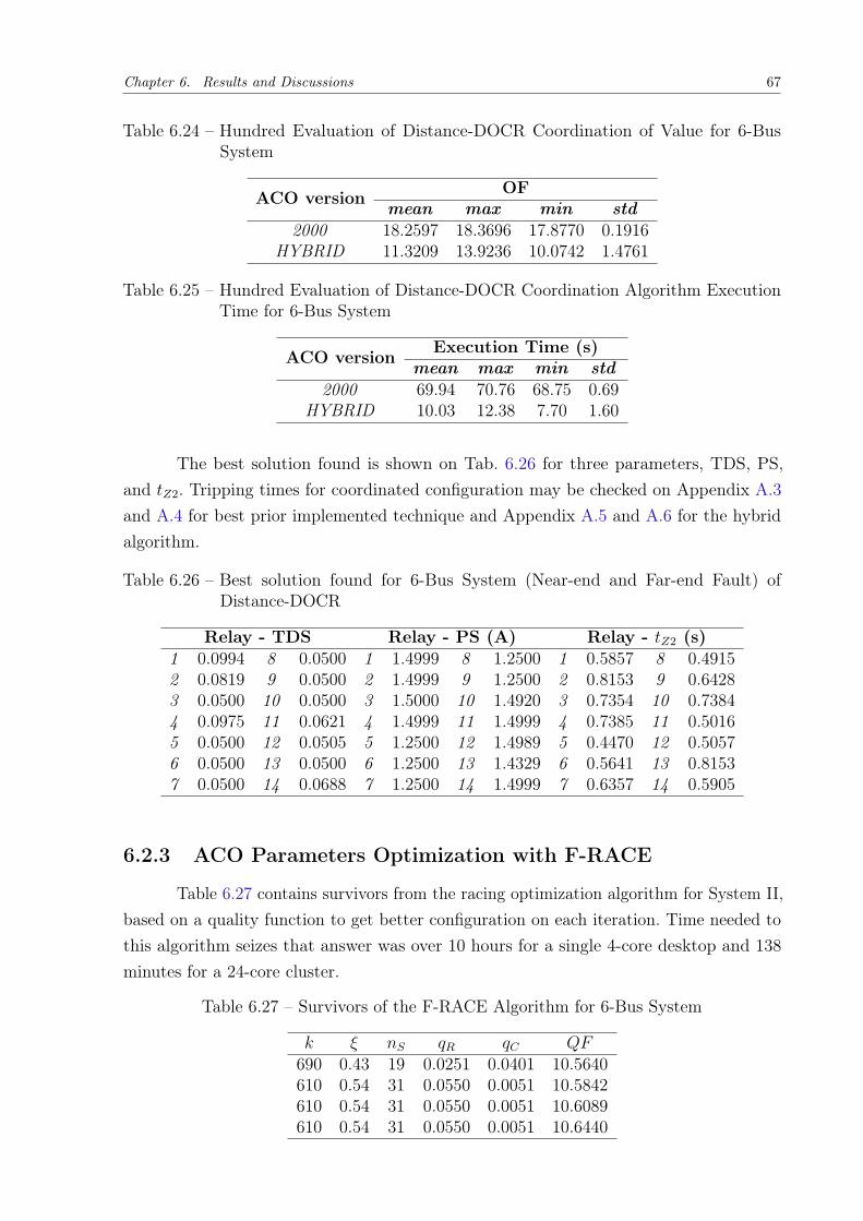
Chapter 6. Results and Discussions 67
Table 6.24 – Hundred Evaluation of Distance-DOCR Coordination of Value for 6-BusSystem
ACO version OFmean max min std
2000 18.2597 18.3696 17.8770 0.1916HYBRID 11.3209 13.9236 10.0742 1.4761
Table 6.25 – Hundred Evaluation of Distance-DOCR Coordination Algorithm ExecutionTime for 6-Bus System
ACO version Execution Time (s)mean max min std
2000 69.94 70.76 68.75 0.69HYBRID 10.03 12.38 7.70 1.60
The best solution found is shown on Tab. 6.26 for three parameters, TDS, PS,and tZ2. Tripping times for coordinated configuration may be checked on Appendix A.3and A.4 for best prior implemented technique and Appendix A.5 and A.6 for the hybridalgorithm.
Table 6.26 – Best solution found for 6-Bus System (Near-end and Far-end Fault) ofDistance-DOCR
Relay - TDS Relay - PS (A) Relay - tZ2 (s)1 0.0994 8 0.0500 1 1.4999 8 1.2500 1 0.5857 8 0.49152 0.0819 9 0.0500 2 1.4999 9 1.2500 2 0.8153 9 0.64283 0.0500 10 0.0500 3 1.5000 10 1.4920 3 0.7354 10 0.73844 0.0975 11 0.0621 4 1.4999 11 1.4999 4 0.7385 11 0.50165 0.0500 12 0.0505 5 1.2500 12 1.4989 5 0.4470 12 0.50576 0.0500 13 0.0500 6 1.2500 13 1.4329 6 0.5641 13 0.81537 0.0500 14 0.0688 7 1.2500 14 1.4999 7 0.6357 14 0.5905
6.2.3 ACO Parameters Optimization with F-RACE
Table 6.27 contains survivors from the racing optimization algorithm for System II,based on a quality function to get better configuration on each iteration. Time needed tothis algorithm seizes that answer was over 10 hours for a single 4-core desktop and 138minutes for a 24-core cluster.
Table 6.27 – Survivors of the F-RACE Algorithm for 6-Bus System
k ξ nS qR qC QF690 0.43 19 0.0251 0.0401 10.5640610 0.54 31 0.0550 0.0051 10.5842610 0.54 31 0.0550 0.0051 10.6089610 0.54 31 0.0550 0.0051 10.6440
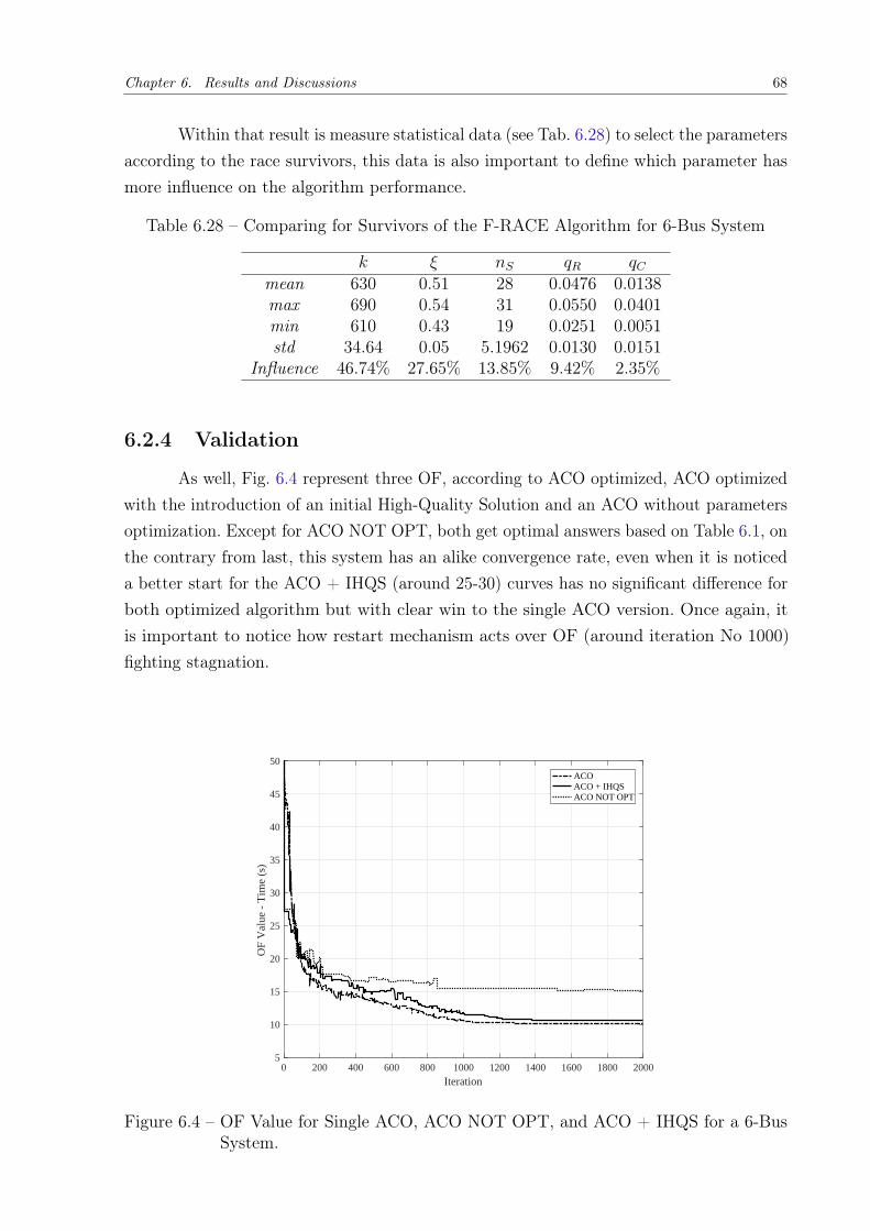
Chapter 6. Results and Discussions 68
Within that result is measure statistical data (see Tab. 6.28) to select the parametersaccording to the race survivors, this data is also important to define which parameter hasmore influence on the algorithm performance.
Table 6.28 – Comparing for Survivors of the F-RACE Algorithm for 6-Bus System
k ξ nS qR qCmean 630 0.51 28 0.0476 0.0138max 690 0.54 31 0.0550 0.0401min 610 0.43 19 0.0251 0.0051std 34.64 0.05 5.1962 0.0130 0.0151
Influence 46.74% 27.65% 13.85% 9.42% 2.35%
6.2.4 Validation
As well, Fig. 6.4 represent three OF, according to ACO optimized, ACO optimizedwith the introduction of an initial High-Quality Solution and an ACO without parametersoptimization. Except for ACO NOT OPT, both get optimal answers based on Table 6.1, onthe contrary from last, this system has an alike convergence rate, even when it is noticeda better start for the ACO + IHQS (around 25-30) curves has no significant difference forboth optimized algorithm but with clear win to the single ACO version. Once again, itis important to notice how restart mechanism acts over OF (around iteration No 1000)fighting stagnation.
0 200 400 600 800 1000 1200 1400 1600 1800 2000
Iteration
5
10
15
20
25
30
35
40
45
50
OF
Val
ue -
Tim
e (s
)
ACOACO + IHQSACO NOT OPT
Figure 6.4 – OF Value for Single ACO, ACO NOT OPT, and ACO + IHQS for a 6-BusSystem.

Chapter 6. Results and Discussions 69
OF value from ACO-LP for a 6-Bus System shows in Fig. 6.5 and Fig. 6.6 fastconvergence in few iterations into optimal value for both DOCRs Only and Distance-DOCRCoordination.
1 2 3 4 5 6 7 8 9 10
Iteration
10
20
30
40
50
60
70
80
90
OF
Val
ue -
Tim
e (s
)
ACO-LP
Figure 6.5 – OF value DOCR Coordination with ACO-LP for a 6-Bus System
1 2 3 4 5 6 7 8 9 10
Iteration
10
20
30
40
50
60
70
80
90
OF
Val
ue -
Tim
e (s
)
ACO-LP
Figure 6.6 – OF value Distance-DOCR Coordination with ACO-LP for a 6-Bus System
ACO-LP algorithm applied to System II obtained the best solution for this problem(OF = 10.0742) in 11.87 s compare to GA (SWIEF et al., 2015), Modified DifferentialEvolution (MDE) (CHELLIAH et al., 2014), MDE5 (THANGARAJ et al., 2010), andOpposition Based Chaotic Differential Evolution (OCDE) (CHELLIAH et al., 2014)GACB-LP (KIDA, 2016). A complete chart is shown in Table 6.29.

Chapter 6. Results and Discussions 70
Table 6.29 – Results Comparison for 6-Bus System Mid-Point Fault DOCR
Tech Autor Exe Time (s) OF - Time (s)GA (SWIEF et al., 2015) - 10.7345MDE (CHELLIAH et al., 2014) 129.80 10.6272MDE5 (THANGARAJ et al., 2010) - 10.3514OCDE (CHELLIAH et al., 2014) 10.14 10.3286
ACO-MV This Work 100.07 10.1584GACB-LP (KIDA, 2016) 89.09 10.1512ACO-LP This Work 11.87 10.0742
Distance-DOCR coordination based on Near-end and Far-end Fault was not possibleto validate with literature, in order to build this model must be assumed fault locationsto distinguish Primary-Backup for this mixed scheme. Data from Table 6.26 shows limitaccording to Table 3.5.
6.3 System III: Eight Bus Network
For System III, there is only one possible configuration Near-end Faults to apply asimple DOCRs Coordination and also a combined scheme with Distance Relays. For thissystem comparing with other meta-heuristic techniques in the literature is also offered.
6.3.1 DOCRs Only
The algorithm runs a hundred times with four different configurations evaluatingOF value (See Tab. 6.30) and Execution time (See Tab. 6.31). Those configurations areOptimized ACOMV for 10000 Iterations, an additional 10000 iterations using an IHQS, anACOMV with not optimized parameters, and a Hybrid configuration based on ACO−LP .
Table 6.30 – Hundred Evaluation of DOCR Objective Function Value for 8-Bus System
ACO version OFmean max min std
10000 10.1028 11.0182 9.2719 0.3657NOT OPT 16.7339 23.6919 11.8787 2.7388
10000 + IHQS 8.9794 9.0526 8.8609 0.0281HYBRID 8.4910 8.6423 8.4271 0.0588

Chapter 6. Results and Discussions 71
Table 6.31 – Hundred Evaluation of DOCR Algorithm Execution Time for 8-Bus System
ACO version Execution Time (s)mean max min std
10000 68.34 82.82 66.43 2.53NOT OPT 34.65 42.50 25.01 3.23
10000 + IHQS 0.40 1.28 0.23 0.17HYBRID 7.77 11.02 6.62 0.94
The best solution found occurs under ACO − LP scenario and is shown on Tab.6.32. Tripping times for coordinated configuration may be checked on Appendix A.7 forbest prior implemented technique and Appendix A.8 for the hybrid algorithm.
Table 6.32 – Best solution found for 8-Bus System (Near-end Fault) of DOCR
Relay - TDS Relay - PS (A)1 0.1131 8 0.1696 1 2 8 2.52 0.2602 9 0.1472 2 2.5 9 2.53 0.2251 10 0.1758 3 2.5 10 2.54 0.1602 11 0.1868 4 2.5 11 2.55 0.1 12 0.2663 5 2.5 12 2.56 0.1731 13 0.1138 6 2.5 13 27 0.2427 14 0.2458 7 2.5 14 2.5
Exhaustive Reduced Space Search for 8-bus System
Total Search Space (TSS) for eight-bus system is 6.78E+11 LP to solve with onlyseven PSs available and fourteen relays to configure. If reduced only to feasible PS between1.5 and 2.5 Valid Search Space (VSS) decrease to 4782969. Those numbers are possibleto compute for this kind of system, results for 10 best solutions are shown in Table 6.33,respectively. The best configuration found is equal to proposed algorithm.
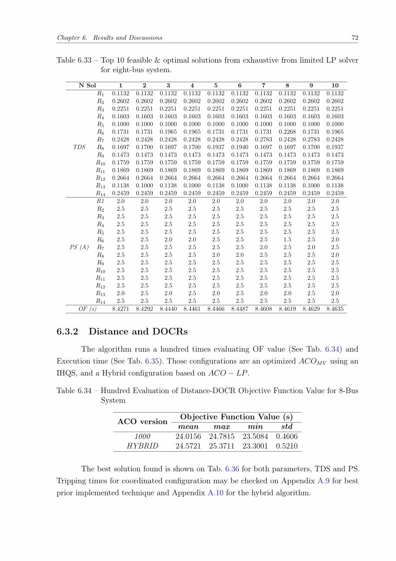
Chapter 6. Results and Discussions 72
Table 6.33 – Top 10 feasible & optimal solutions from exhaustive from limited LP solverfor eight-bus system.
N Sol 1 2 3 4 5 6 7 8 9 10R1 0.1132 0.1132 0.1132 0.1132 0.1132 0.1132 0.1132 0.1132 0.1132 0.1132
TDS
R2 0.2602 0.2602 0.2602 0.2602 0.2602 0.2602 0.2602 0.2602 0.2602 0.2602R3 0.2251 0.2251 0.2251 0.2251 0.2251 0.2251 0.2251 0.2251 0.2251 0.2251R4 0.1603 0.1603 0.1603 0.1603 0.1603 0.1603 0.1603 0.1603 0.1603 0.1603R5 0.1000 0.1000 0.1000 0.1000 0.1000 0.1000 0.1000 0.1000 0.1000 0.1000R6 0.1731 0.1731 0.1965 0.1965 0.1731 0.1731 0.1731 0.2268 0.1731 0.1965R7 0.2428 0.2428 0.2428 0.2428 0.2428 0.2428 0.2783 0.2428 0.2783 0.2428R8 0.1697 0.1700 0.1697 0.1700 0.1937 0.1940 0.1697 0.1697 0.1700 0.1937R9 0.1473 0.1473 0.1473 0.1473 0.1473 0.1473 0.1473 0.1473 0.1473 0.1473R10 0.1759 0.1759 0.1759 0.1759 0.1759 0.1759 0.1759 0.1759 0.1759 0.1759R11 0.1869 0.1869 0.1869 0.1869 0.1869 0.1869 0.1869 0.1869 0.1869 0.1869R12 0.2664 0.2664 0.2664 0.2664 0.2664 0.2664 0.2664 0.2664 0.2664 0.2664R13 0.1138 0.1000 0.1138 0.1000 0.1138 0.1000 0.1138 0.1138 0.1000 0.1138R14 0.2459 0.2459 0.2459 0.2459 0.2459 0.2459 0.2459 0.2459 0.2459 0.2459
PS (A)
R1 2.0 2.0 2.0 2.0 2.0 2.0 2.0 2.0 2.0 2.0R2 2.5 2.5 2.5 2.5 2.5 2.5 2.5 2.5 2.5 2.5R3 2.5 2.5 2.5 2.5 2.5 2.5 2.5 2.5 2.5 2.5R4 2.5 2.5 2.5 2.5 2.5 2.5 2.5 2.5 2.5 2.5R5 2.5 2.5 2.5 2.5 2.5 2.5 2.5 2.5 2.5 2.5R6 2.5 2.5 2.0 2.0 2.5 2.5 2.5 1.5 2.5 2.0R7 2.5 2.5 2.5 2.5 2.5 2.5 2.0 2.5 2.0 2.5R8 2.5 2.5 2.5 2.5 2.0 2.0 2.5 2.5 2.5 2.0R9 2.5 2.5 2.5 2.5 2.5 2.5 2.5 2.5 2.5 2.5R10 2.5 2.5 2.5 2.5 2.5 2.5 2.5 2.5 2.5 2.5R11 2.5 2.5 2.5 2.5 2.5 2.5 2.5 2.5 2.5 2.5R12 2.5 2.5 2.5 2.5 2.5 2.5 2.5 2.5 2.5 2.5R13 2.0 2.5 2.0 2.5 2.0 2.5 2.0 2.0 2.5 2.0R14 2.5 2.5 2.5 2.5 2.5 2.5 2.5 2.5 2.5 2.5
OF (s) 8.4271 8.4292 8.4440 8.4461 8.4466 8.4487 8.4608 8.4619 8.4629 8.4635
6.3.2 Distance and DOCRs
The algorithm runs a hundred times evaluating OF value (See Tab. 6.34) andExecution time (See Tab. 6.35). Those configurations are an optimized ACOMV using anIHQS, and a Hybrid configuration based on ACO − LP .
Table 6.34 – Hundred Evaluation of Distance-DOCR Objective Function Value for 8-BusSystem
ACO version Objective Function Value (s)mean max min std
1000 24.0156 24.7815 23.5084 0.4606HYBRID 24.5721 25.3711 23.3001 0.5210
The best solution found is shown on Tab. 6.36 for both parameters, TDS and PS.Tripping times for coordinated configuration may be checked on Appendix A.9 for bestprior implemented technique and Appendix A.10 for the hybrid algorithm.
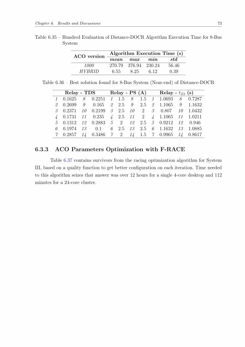
Chapter 6. Results and Discussions 73
Table 6.35 – Hundred Evaluation of Distance-DOCR Algorithm Execution Time for 8-BusSystem
ACO version Algorithm Execution Time (s)mean max min std
1000 270.79 376.94 230.24 56.46HYBRID 6.55 8.25 6.12 0.39
Table 6.36 – Best solution found for 8-Bus System (Near-end) of Distance-DOCR
Relay - TDS Relay - PS (A) Relay - tZ2 (s)1 0.1625 8 0.2251 1 1.5 8 1.5 1 1.0693 8 0.72872 0.2699 9 0.165 2 2.5 9 2.5 2 1.1065 9 1.16323 0.2371 10 0.2199 3 2.5 10 2 3 0.807 10 1.04324 0.1731 11 0.235 4 2.5 11 2 4 1.1065 11 1.02115 0.1312 12 0.2883 5 2 12 2.5 5 0.9212 12 0.9466 0.1974 13 0.1 6 2.5 13 2.5 6 1.1632 13 1.08857 0.2857 14 0.3486 7 2 14 1.5 7 0.9965 14 0.8617
6.3.3 ACO Parameters Optimization with F-RACE
Table 6.37 contains survivors from the racing optimization algorithm for SystemIII, based on a quality function to get better configuration on each iteration. Time neededto this algorithm seizes that answer was over 12 hours for a single 4-core desktop and 112minutes for a 24-core cluster.
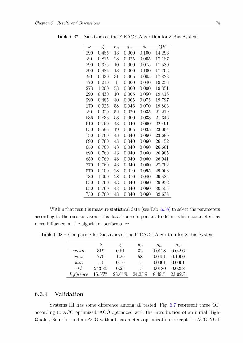
Chapter 6. Results and Discussions 74
Table 6.37 – Survivors of the F-RACE Algorithm for 8-Bus System
k ξ nS qR qC QF290 0.485 13 0.000 0.100 14.29650 0.815 28 0.025 0.005 17.187290 0.375 10 0.000 0.075 17.580290 0.485 13 0.000 0.100 17.70690 0.430 31 0.005 0.005 17.823170 0.210 1 0.000 0.040 19.258273 1.200 53 0.000 0.000 19.351290 0.430 10 0.005 0.050 19.416290 0.485 40 0.005 0.075 19.797170 0.925 58 0.045 0.070 19.80650 0.320 52 0.020 0.035 21.219536 0.833 53 0.000 0.033 21.346610 0.760 43 0.040 0.060 22.491650 0.595 19 0.005 0.035 23.004730 0.760 43 0.040 0.060 23.686690 0.760 43 0.040 0.060 26.452650 0.760 43 0.040 0.060 26.601690 0.760 43 0.040 0.060 26.905650 0.760 43 0.040 0.060 26.941770 0.760 43 0.040 0.060 27.702570 0.100 28 0.010 0.095 29.003130 1.090 28 0.010 0.040 29.585650 0.760 43 0.040 0.060 29.952650 0.760 43 0.040 0.060 30.555730 0.760 43 0.040 0.060 32.638
Within that result is measure statistical data (see Tab. 6.38) to select the parametersaccording to the race survivors, this data is also important to define which parameter hasmore influence on the algorithm performance.
Table 6.38 – Comparing for Survivors of the F-RACE Algorithm for 8-Bus System
k ξ nS qR qCmean 319 0.61 32 0.0128 0.0496max 770 1.20 58 0.0451 0.1000min 50 0.10 1 0.0001 0.0001std 243.85 0.25 15 0.0180 0.0258
Influence 15.65% 28.61% 24.23% 8.49% 23.02%
6.3.4 Validation
Systems III has some difference among all tested, Fig. 6.7 represent three OF,according to ACO optimized, ACO optimized with the introduction of an initial High-Quality Solution and an ACO without parameters optimization. Except for ACO NOT

Chapter 6. Results and Discussions 75
OPT which does not even shows a convergence characteristic, in this occasion ACO,obtain good quality solution as shown in Table 6.47, this system only shows an expectedconvergence rate for the ACO single version, it is noticed a better start for the ACO +IHQS but reduced after few iterations keeping trapped into a minimum better althoughother algorithm. For this System is also added Fig. 6.8 correspondent to Unfitness, showinghow important is parameter optimization for this case.
0 500 1000 1500 2000 2500 3000
Iteration
8
10
12
14
16
18
20
22
24
26
OF
Val
ue -
Tim
e (s
)
ACOACO + IHQSACO NOT OPT
Figure 6.7 – OF Value for Single ACO, ACO NOT OPT, and ACO + IHQS for a 8-BusSystem.

Chapter 6. Results and Discussions 76
0 500 1000 1500 2000 2500 3000
Iteration
-5
0
5
10
15
20
25
30
35
40
OF
Val
ue -
Tim
e (s
)
ACOACO + IHQSACO NOT OPT
Figure 6.8 – Unfitness Value for Single ACO, ACO NOT OPT, and ACO + IHQS for a8-Bus System.
OF value from ACO-LP for a 8-Bus System shows in Fig. 6.9 fast convergence infew iterations into optimal value for both DOCRs Only and Distance-DOCR Coordination.
1 2 3 4 5 6 7 8 9 10
Iteration
8
8.5
9
9.5
10
10.5
11
11.5
OF
Val
ue -
Tim
e (s
)
ACO-LP
Figure 6.9 – OF Value for DOCR Coordination with ACO-LP for a 8-Bus System.

Chapter 6. Results and Discussions 77
1 2 3 4 5 6 7 8 9 10
Iteration
23.2
23.4
23.6
23.8
24
24.2
24.4
24.6
24.8
OF
Val
ue -
Tim
e (s
)
ACO-LP
Figure 6.10 – OF Value for Distance-DOCR Coordination with ACO-LP for a 8-BusSystem.
ACO-MV algorithm applied to System III obtained a better solution for thisproblem (OF = 8.8609) in 0.23 s than GA, GA-NLP (NOGHABI et al., 2009), BBO(ALBASRI et al., 2015)„ OSL Solver (OSL) (ZEINELDIN et al., 2005) and worst thanGACB-LP (KIDA, 2016) or SOA (AMRAEE, 2012). ACO-LP algorithm applied to SystemIII obtained the best solution for this problem (OF = 8.4271) in 7.07 s. A complete chartis shown in Table 6.39.
Table 6.39 – Results Comparison for 8-Bus System Fault DOCR
Tech Autor Exe Time (s) OF - Time (s)OSL (ZEINELDIN et al., 2005) - 17.33GA (NOGHABI et al., 2009) 36000.00 11.001
GA-PL (NOGHABI et al., 2009) 300.00 10.949BBO (ALBASRI et al., 2015) 2065.02 10.5495
ACO-MV This Work 0.23 8.8609BBO-LP (ALBASRI et al., 2015) 6.79 8.7556SOA (AMRAEE, 2012) 50.45 8.4271
GACB-LP (KIDA, 2016) 0.20 8.4271ACO-LP This Work 7.07 8.4271
6.4 System IV: Nine Bus Network
For System IV, the configuration is given for a Mid-Point Faults to apply a simpleDOCRs Coordination. For this system validation with other meta-heuristic techniques inthe literature are considered.

Chapter 6. Results and Discussions 78
6.4.1 DOCRs Only
The algorithm runs a hundred times with four different configurations evaluatingOF value (See Tab. 6.40) and Execution time (See Tab. 6.41). Those configurations areOptimized ACOMV for 10000 Iterations, an additional 10000 iterations using an IHQS,also presented an ACOMV with not optimized parameters, and a Hybrid configurationbased on ACO − LP .
Table 6.40 – Hundred Evaluation of DOCR Objective Function Value for 9-Bus System
ACO version OFmean max min std
10000 5.3882 6.3056 4.9125 0.2935NOT OPT 19.4870 34.6103 13.3393 5.0521
10000 + IHQS 5.0536 5.4200 4.8017 0.1399HYBRID 6.3506 6.9108 5.8713 0.2102
Table 6.41 – Hundred Evaluation of DOCR Algorithm Execution Time for 9-Bus System
ACO version Execution Time (s)mean max min std
10000 127.78 1280.16 90.42 116.94NOT OPT 133.40 277.13 43.41 50.43
10000 + IHQS 41.99 67.56 39.97 2.72HYBRID 21.32 34.17 18.83 2.08
The best solution found occurs under 10000 iteration using an IHQS scenario andis shown on Tab. 6.42 and Tab. 6.43. Tripping times for coordinated configuration may bechecked on Appendix A.11 for best prior implemented technique and Appendix A.12 forthe hybrid algorithm.
Table 6.42 – Best TDS solution found for 9-Bus System (Near-end and Far-end Fault) ofDOCR
Relay - TDS1 0.0676 9 0.0445 17 0.06802 0.0402 10 0.0523 18 0.04033 0.0326 11 0.0407 19 0.07364 0.0341 12 0.0384 20 0.04645 0.0312 13 0.0586 21 0.06896 0.0621 14 0.0604 22 0.03987 0.0529 15 0.0733 23 0.07378 0.0340 16 0.0398 24 0.0279

Chapter 6. Results and Discussions 79
Table 6.43 – Best PS solution found for 9-Bus System (Near-end and Far-end Fault) ofDOCR
Relay - PS (A)1 0.9646 9 1.1280 17 1.48922 0.8170 10 0.9326 18 1.13113 1.8190 11 0.8037 19 1.20774 1.6054 12 1.4919 20 1.06255 1.2099 13 0.9893 21 1.44686 1.0420 14 1.0536 22 1.15447 1.4229 15 0.6847 23 1.27918 1.0990 16 1.8674 24 1.2665
6.4.2 ACO Parameters Optimization with F-RACE
Table 6.44 contains survivors from the racing optimization algorithm for System IV,based on a quality function to get a better configuration on each iteration. Time neededto this algorithm seizes that answer was over 72 hours for a single 4-core desktop and 11hours for a 24-core cluster.
Table 6.44 – Survivors of the F-RACE Algorithm for 9-Bus System
k ξ nS qR qC QF650 0.705 40 0.0950 0.0051 8.2579610 0.760 40 0.0900 0.0051 8.2643610 0.760 40 0.0900 0.0051 8.2645570 0.760 40 0.0950 0.0051 8.2646610 0.760 37 0.0850 0.0001 8.2656610 0.760 40 0.0850 0.0001 8.2659610 0.760 40 0.0850 0.0001 8.2696610 0.760 37 0.0950 0.0051 8.2874650 0.760 40 0.1000 0.0001 8.2964570 0.760 40 0.0900 0.0151 8.3029650 0.760 37 0.0950 0.0101 8.3169610 0.760 37 0.0950 0.0051 8.3850610 0.815 43 0.0850 0.0101 8.5485650 0.815 40 0.1000 0.0001 8.7108610 0.815 40 0.0950 0.0101 8.7178610 0.815 40 0.0900 0.0051 8.7479570 0.815 34 0.0950 0.0051 8.8072570 0.815 37 0.0900 0.0051 9.0201690 0.815 43 0.1000 0.0101 9.4548690 0.815 40 0.0950 0.0051 9.6279
Within that result is measure statistical data (see Tab. 6.45) to select the parametersaccording to the race survivors, this data is also important to define which parameter hasmore influence on the algorithm performance.

Chapter 6. Results and Discussions 80
Table 6.45 – Comparing for Survivors of the F-RACE Algorithm for 9-Bus System
k ξ nS qR qCmean 618 0.779 39 0.0925 0.0053max 690 0.815 43 0.1000 0.0151min 570 0.705 34 0.0850 0.0001std 34.87 0.031 2 0.0049 0.0040
Influence 21.73% 30.36% 22.98% 23.30% 1.63%
6.4.3 Validation
As well, Fig. 6.11 represent three OF, according to ACO optimized, ACO optimizedwith the introduction of an initial High-Quality Solution and an ACO without parametersoptimization. Except for ACO NOT OPT, in this occasion ACO, obtain good qualitysolution as shown in Table 6.40, compare to System I, this system has an alike initialconvergence rate, it is noticed a better start for the ACO + IHQS but after 3000 iterationsthere is no significant difference for both optimized algorithm but with clear win to theACO with IHQS. Once again, It is important to notice how restart mechanism acts over OF(around iteration No 1000 for ACO+IHQS and 2500 for single ACO) fighting stagnation.
0 1000 2000 3000 4000 5000 6000 7000 8000 9000 10000
Iteration
0
10
20
30
40
50
60
OF
Val
ue -
Tim
e (s
)
ACOACO + IHQSACO NOT OPT
Figure 6.11 – OF Value for Single ACO, ACO NOT OPT, and ACO + IHQS for a 9-BusSystem.
The output from Distance-DOCR Coordination with ACO-LP for a 9-Bus System(Fig. ??), shows an difference convergence rate in the OF value until configuration entersinto the feasible region.

Chapter 6. Results and Discussions 81
5 10 15 20 25 30
Iteration
4
5
6
7
8
9
10
11
12
13
OF
Val
ue -
Tim
e (s
)
ACO-LP
Figure 6.12 – OF Value of DOCR Coordination with ACO-LP for a 9-Bus System.
5 10 15 20 25 30
Iteration
-0.5
0
0.5
1
1.5
2
Unf
itnes
s -
Tim
e (s
)
ACO-LP
Figure 6.13 – Unfitness Value of DOCR Coordination with ACO-LP for a 9-Bus System.
ACO-MV and ACO-LP algorithm applied to System IV obtained better solutionsfor this problem (OF = 4.8017 and OF = 5.8713) in 40.19 s and 18.83 s, respectively,compare toGA, GA-NLP, Sequential Quadratic Programming (SQP) (BEDEKAR; BHIDE,2011a), and BBO (ALBASRI et al., 2015) and close but worst than GACB-LP (KIDA,2016) and BBO-LP (ALBASRI et al., 2015). A complete chart is shown in Table 6.46. OFwill be limited to 4.8 s due to Tmin constraint for relay minimum time 0.2 s.

Chapter 6. Results and Discussions 82
Table 6.46 – Results Comparison for 9-Bus System Fault DOCR
Tech Autor Exe Time (s) OF - Time (s)GA (BEDEKAR; BHIDE, 2011a) - 32.6058BBO (ALBASRI et al., 2015) - 28.8348SQP (BEDEKAR; BHIDE, 2011a) - 19.4041
GA-NLP (BEDEKAR; BHIDE, 2011a) - 6.1786ACO-LP This Work 18.83 5.8713ACO-MV This Work 40.19 4.8017BBO-LP (ALBASRI et al., 2015) - 4.8000GACB-LP (KIDA, 2016) 4.11 4.8000
6.5 System V: Fifteen Bus Network
For System V, the configuration is given for a Mid-Point Faults to apply a simpleDOCRs Coordination. For this system validation with other meta-heuristic techniques inthe literature are considered.
6.5.1 DOCRs Only
The algorithm runs a hundred times with four different configurations evaluatingOF value (See Tab. 6.47) and Execution time (See Tab. 6.48. Those configurations areOptimized ACOMV for 10000 Iterations, an additional 10000 iterations using an IHQS,within an ACOMV with not optimized parameters, and a Hybrid configuration based onACO − LP .
Table 6.47 – Hundred Evaluation of DOCR Objective Function Value for 15-Bus System
ACO version OFmean max min std
10000 15.5769 16.8223 14.5381 0.4862NOT OPT 64.3561 66.4206 59.9903 2.3812
10000 + IHQS 13.9052 13.9052 13.9052 0.0000HYBRID 12.9878 13.2660 12.7001 0.1232
Table 6.48 – Hundred Evaluation of DOCR Algorithm Execution Time for 15-Bus System
ACO version Execution Time (s)mean max min std
10000 472.14 506.49 464.46 13.83NOT OPT 597.51 757.83 491.31 94.22
10000 + IHQS 0.58 1.75 0.63 0.00HYBRID 13.20 28.62 11.22 2.57
The best solution found occurs under ACO−LP scenario and is shown on Tab. 6.49and Tab. 6.50. Tripping times for coordinated configuration may be checked on AppendixA.13 for best prior implemented technique and Appendix A.14 for the hybrid algorithm.

Chapter 6. Results and Discussions 83
Table 6.49 – Best TDS solution found for 15-Bus System (Near-end and Far-end Fault) ofDOCR
Relay - TDS1 0.1000 12 0.1315 23 0.1103 34 0.11112 0.1042 13 0.1000 24 0.1063 35 0.10003 0.1000 14 0.1128 25 0.1061 36 0.10004 0.1165 15 0.1055 26 0.1186 37 0.12225 0.1034 16 0.1022 27 0.1069 38 0.10626 0.1000 17 0.1000 28 0.1105 39 0.10397 0.1082 18 0.1000 29 0.1076 40 0.10438 0.10000 19 0.1000 30 0.1000 41 0.10419 0.1082 20 0.1000 31 0.1000 42 0.106710 0.1021 21 0.1116 32 0.100011 0.1000 22 0.1157 33 0.1016
Table 6.50 – Best PS solution found for 15-Bus System (Near-end and Far-end Fault) ofDOCR
Relay - PS (A)1 1.5 12 1.0 23 1.0 34 2.52 1.0 13 2.5 24 1.5 35 2.53 2.5 14 1.0 25 2.0 36 2.04 1.0 15 1.0 26 1.5 37 2.05 2.5 16 1.5 27 2.0 38 2.56 2.5 17 2.5 28 2.5 39 2.57 1.0 18 1.5 29 1.5 40 2.58 2.0 19 2.0 30 2.0 41 2.59 2.0 20 2.0 31 2.5 42 1.510 2.0 21 1.0 32 2.011 2.0 22 1.5 33 2.5
6.5.2 ACO Parameters Optimization with F-RACE
Table 6.51 contains survivors from the racing optimization algorithm for System V,based on a quality function to get better configuration on each iteration. Time needed tothis algorithm seizes that answer was over 120 hours for a single 4-core desktop and 21hours for a 24-core cluster.

Chapter 6. Results and Discussions 84
Table 6.51 – Survivors of the F-RACE Algorithm for 15-Bus System
k ξ nS qR qC QF250 0.650 19 0.0001 0.0750 23.3422410 0.595 19 0.0001 0.0800 27.9935330 0.650 19 0.0001 0.0850 30.3546170 0.375 31 0.0501 0.0001 57.0303170 0.375 28 0.0550 0.0301 67.8027170 0.375 28 0.0550 0.0301 67.8027450 0.210 37 0.0351 0.0001 67.8235450 0.210 37 0.0351 0.0001 67.8235210 0.925 49 0.0351 0.0051 82.9106210 0.925 49 0.0351 0.0051 82.9106
Within that result is measure statistical data (see Tab. 6.52) to select the parametersaccording to the race survivors, this data is also important to define which parameter hasmore influence on the algorithm performance.
Table 6.52 – Comparing for Survivors of the F-RACE Algorithm for 15-Bus System
k ξ nS qR qCmean 282 0.529 31.6 0.0301 0.0311max 450 0.925 49 0.0550 0.0850min 170 0.210 19 0.0001 0.0001std 111.43 0.249 10.8 0.0211 0.0339
Influence 25.51% 21.38% 29.49% 14.38% 9.25%
6.5.3 Validation
To keep in line with last Systems, Fig. 6.14 represent three OF, according to ACOoptimized, ACO optimized with the introduction of an initial High-Quality Solution and anACO without parameters optimization. Except for ACO NOT OPT which does not evenshows a convergence characteristic, in this occasion ACO, obtain good quality solution asshown in Table 6.47, this system only shows an expected convergence rate for the ACOsingle version, it is noticed a better start for the ACO + IHQS but reduced after fewiterations keeping trapped into a minimum better although other algorithm.
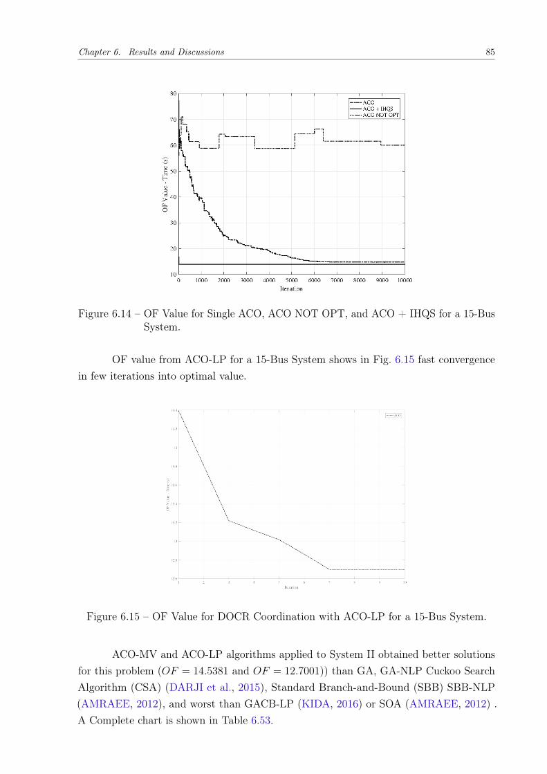
Chapter 6. Results and Discussions 85
Figure 6.14 – OF Value for Single ACO, ACO NOT OPT, and ACO + IHQS for a 15-BusSystem.
OF value from ACO-LP for a 15-Bus System shows in Fig. 6.15 fast convergencein few iterations into optimal value.
Figure 6.15 – OF Value for DOCR Coordination with ACO-LP for a 15-Bus System.
ACO-MV and ACO-LP algorithms applied to System II obtained better solutionsfor this problem (OF = 14.5381 and OF = 12.7001)) than GA, GA-NLP Cuckoo SearchAlgorithm (CSA) (DARJI et al., 2015), Standard Branch-and-Bound (SBB) SBB-NLP(AMRAEE, 2012), and worst than GACB-LP (KIDA, 2016) or SOA (AMRAEE, 2012) .A Complete chart is shown in Table 6.53.

Chapter 6. Results and Discussions 86
Table 6.53 – Results Comparison for 15-Bus System Mid-Point Fault DOCR
Tech Autor Exe Time (s) OF - Time (s)GA (DARJI et al., 2015) - 35.8812
GA-NLP (DARJI et al., 2015) - 19.5843CSA (DARJI et al., 2015) - 19.5521SBB (AMRAEE, 2012) - 15.3350
SBB-NLP (AMRAEE, 2012) 60.70 15.0020ACO-MV This Work 0.63 14.5381ACO-LP This Work 11.22 12.7001
SOA (AMRAEE, 2012) 406.30 12.2270GACB-LP (KIDA, 2016) 5.11 12.2149
6.6 Discussions and Final Considerations
The IHQS open a debate due to how fast locates good sub-optimal solutions, evenafter some ACO iterations there is no guarantee of finding better solutions but an initialfeasible space. In general would be possible using directly a technique based on LP to geta system coordinated in a fraction of the time required by a heuristic technique. Hybridapproach validate last statement improving almost every single value for all systemsapplications.
F-RACE algorithm has additional information to be considered for applicationwhere computing time for optimization is no longer available and a tunning must beperformed as fast as possible. Table 6.54 shows a percentage relation between the standarddeviation and the mean value per parameter for each system tested. Table 6.54 marksthe parameters influence under our solution, saying that there are two parameters with anotorious qualification, ξ the convergence parameter of the algorithm is most importantvalue to be configured, only follow by nS the number of ants working to build new solutions.Those parameters are important not only to find a high-quality solution but improve theperformance of the algorithm. On the contrary, qC is the parameter which no requires aspecific configuration.
Table 6.54 – Parameter influence for all tested system
System k ξ nS qR qC3-BUS 13.18% 31.38% 23.37% 20.16% 11.90%6-BUS 46.74% 27.65% 13.85% 9.42% 2.35%8-BUS 15.65% 28.61% 24.23% 8.49% 23.02%9-BUS 21.73% 30.36% 22.98% 23.30% 1.63%15-BUS 25.51% 21.38% 29.49% 14.38% 9.25%
Corroborate the advantage of parallel programming providing concurrency, per-forming simultaneously multiple actions at the same time, reducing execution time.
Besides, there are difference contingency scenarios where relay settings should (or

Chapter 6. Results and Discussions 87
could) not be reset (e.g. utility requirements or communication failure) and coordinationis made disabling constraints where those relays are present finding a new suboptimalanswer but feasible.
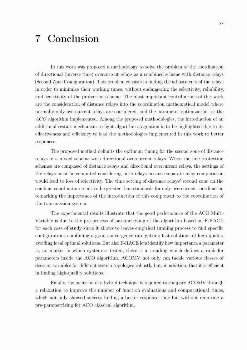
88
7 Conclusion
In this work was proposed a methodology to solve the problem of the coordinationof directional (inverse time) overcurrent relays as a combined scheme with distance relays(Second Zone Configuration). This problem consists in finding the adjustments of the relaysin order to minimize their working times, without endangering the selectivity, reliability,and sensitivity of the protection scheme. The most important contributions of this workare the consideration of distance relays into the coordination mathematical model wherenormally only overcurrent relays are considered, and the parameter optimization for theACO algorithm implemented. Among the proposed methodologies, the introduction of anadditional restart mechanism to fight algorithm stagnation is to be highlighted due to itseffectiveness and efficiency to lead the methodologies implemented in this work to betterresponses.
The proposed method delimits the optimum timing for the second zone of distancerelays in a mixed scheme with directional overcurrent relays. When the line protectionschemes are composed of distance relays and directional overcurrent relays, the settings ofthe relays must be computed considering both relays because separate relay computationwould lead to loss of selectivity. The time setting of distance relays’ second zone on thecombine coordination tends to be greater than standards for only overcurrent coordinationremarking the importance of the introduction of this component to the coordination ofthe transmission system.
The experimental results illustrate that the good performance of the ACO Multi-Variable is due to the pre-process of parametrizing of the algorithm based on F-RACEfor each case of study since it allows to leaves empirical tunning process to find specificconfigurations combining a good convergence rate getting fast solutions of high-qualityavoiding local optimal solutions. But also F-RACE lets identify how importance a parameteris, no matter in which system is tested, there is a trending which defines a rank forparameters inside the ACO algorithm. ACOMV not only can tackle various classes ofdecision variables for different system topologies robustly but, in addition, that it is efficientin finding high-quality solutions.
Finally, the inclusion of a hybrid technique is required to compare ACOMV througha relaxation to improve the number of function evaluations and computational times,which not only showed success finding a better response time but without requiring apre-parametrizing for ACO classical algorithm.

89
8 Recommendations for Future Work
• Application of local non-convex optimization based on piecewise linear approximation.
• Software integration for power flow calculations, short circuits and the parameteriza-tion of relays with optimization techniques.
• Analysis of various fault scenarios and different operating configurations, Plug andPlay considerations.
• Force solving with non-linear techniques for non-convex problem validating withheuristics results.

90
Bibliography
ABDELAZIZ, A. Y.; TALAAT, H. E. A.; NOSSEIR, A. I.; HAJJAR, A. A. Optimalcoordination of overcurrent relays by linear programming: an enhanced problem formulation.In: Proc. 3rd CIGRE Reg. Conf. Arab Ctries. [S.l.: s.n.], 1999. p. 14. Cited on page 9.
ABYANEH, H. A.; KAMANGAR, S. S. H.; RAZAVI, F.; CHABANLOO, R. M. A newgenetic algorithm method for optimal coordination of overcurrent relays in a mixedprotection scheme with distance relays. In: 2008 43rd Int. Univ. Power Eng. Conf. IEEE,2008. p. 1–5. ISBN 978-1-4244-3294-3. Available from Internet: <http://ieeexplore.ieee.org/document/4651442/>. Cited 2 times on page(s) 3 and 9.
ADENSO-DÍAZ, B.; LAGUNA, M. Fine-Tuning of Algorithms Using Fractional Exper-imental Designs and Local Search. Oper. Res., v. 54, n. 1, p. 99–114, feb 2006. ISSN0030-364X. Available from Internet: <http://pubsonline.informs.org/doi/abs/10.1287/opre.1050.0243>. Cited 2 times on page(s) 9 and 39.
AGUERO, J. R.; TAKAYESU, E.; NOVOSEL, D.; MASIELLO, R. Modernizing the Grid:Challenges and Opportunities for a Sustainable Future. IEEE Power Energy Mag., v. 15,n. 3, p. 74–83, may 2017. ISSN 15407977. Cited on page 22.
AHMADI, S.-A.; KARAMI, H.; GHAREHPETIAN, B. Comprehensive coordinationof combined directional overcurrent and distance relays considering miscoordinationreduction. Int. J. Electr. Power Energy Syst., Elsevier Ltd, v. 92, p. 42–52, nov 2017. ISSN01420615. Available from Internet: <http://dx.doi.org/10.1016/j.ijepes.2017.04.008http://linkinghub.elsevier.com/retrieve/pii/S0142061516323134>. Cited on page 7.
AHMARINEJAD, A.; HASANPOUR, S. M.; BABAEI, M.; TABRIZIAN, M. OptimalOvercurrent Relays Coordination in Microgrid Using Cuckoo Algorithm. Energy Procedia,Elsevier B.V., v. 100, n. September, p. 280–286, 2016. ISSN 18766102. Available fromInternet: <http://dx.doi.org/10.1016/j.egypro.2016.10.178>. Cited on page 11.
ALAM, M. N.; DAS, B.; PANT, V. A comparative study of metaheuristic optimizationapproaches for directional overcurrent relays coordination. Electr. Power Syst. Res., ElsevierB.V., v. 128, p. 39–52, nov 2015. ISSN 03787796. Available from Internet: <http://linkinghub.elsevier.com/retrieve/pii/S0378779615001947>. Cited on page 10.
ALBASRI, F. A.; ALROOMI, A. R.; TALAQ, J. H. Optimal Coordination of DirectionalOvercurrent Relays Using Biogeography-Based Optimization Algorithms. IEEE Trans.Power Deliv., v. 30, n. 4, p. 1810–1820, aug 2015. ISSN 0885-8977. Available from Internet:<http://ieeexplore.ieee.org/document/7047892/>. Cited 6 times on page(s) 11, 64, 65,77, 81, and 82.
AMRAEE, T. Coordination of directional overcurrent relays using seeker algorithm. IEEETrans. Power Deliv., v. 27, n. 3, p. 1415–1422, 2012. ISSN 08858977. Cited 9 times onpage(s) 10, 47, 50, 53, 64, 65, 77, 85, and 86.
ANDERSON, P. Protective Device Characteristics. In: Power Syst. Prot. IEEE, 1999.p. 43–96. Available from Internet: <http://ieeexplore.ieee.org/search/srchabstract.jsp?arnumber=5264157>. Cited on page 20.

Bibliography 91
ANDERSON, P. Analysis of Distance Protection. In: Power Syst. Prot. IEEE, 2009. p.379–417. Available from Internet: <http://ieeexplore.ieee.org/search/srchabstract.jsp?arnumber=5264134>. Cited on page 21.
ARREOLA, O.; CONDE, A. Coordinación de relevadores de sobrecorriente con curvas detiempo no convencionales en sistemas eléctricos industriales. 208 p. Dissertation (Master),2014. Cited on page 10.
ATABEKOV, G. The Relay Protection of High Voltage Networks. [S.l.]: Elsevier, 1960.564 p. Cited on page 9.
ATES, Y.; UZUNOGLU, M.; KARAKAS, A.; BOYNUEGRI, A. R.; NADAR, A.; DAG, B.Implementation of adaptive relay coordination in distribution systems including distributedgeneration. J. Clean. Prod., Elsevier Ltd, v. 112, p. 2697–2705, 2016. ISSN 09596526.Available from Internet: <http://dx.doi.org/10.1016/j.jclepro.2015.10.066>. Cited onpage 11.
BALAPRAKASH, P.; BIRATTARI, M.; STUETZLE, T. Hybrid Metaheuristics. Berlin,Heidelberg: Springer Berlin Heidelberg, 2007. v. 4771. 108–122 p. (Lecture Notes inComputer Science, May). ISSN 0302-9743. ISBN 978-3-540-75513-5. Available from Internet:<http://link.springer.com/10.1007/978-3-540-75514-2>. Cited 2 times on page(s) 9and 41.
BALLANTYNE, K.; OORSCHOT, R. van; MITCHELL, R. Reduce optimisation timeand effort: Taguchi experimental design methods. Forensic Sci. Int. Genet. Suppl. Ser.,v. 1, n. 1, p. 7–8, aug 2008. ISSN 18751768. Available from Internet: <http://linkinghub.elsevier.com/retrieve/pii/S1875176808000784>. Cited on page 9.
BARRETO, J. R. O. Coordinación de Protecciones Eléctricas en el sistema de distribucióna nivel de 34,5 kV y 13,8 kV del área pesado, Distrito Morichal, PDVSA. Dissertation(Master) — UNIVERSIDAD DE ORIENTE, 2010. Cited on page 10.
BARTZ-BEIELSTEIN, T.; CHIARANDINI, M.; PAQUETE, L.; PREUSS, M. Experi-mental methods for the analysis of optimization algorithms. Exp. Methods Anal. Optim.Algorithms, p. 1–457, 2010. Cited 2 times on page(s) 9 and 41.
BAYLISS, C.; HARDY, B. Relay Protection. In: Transm. Distrib. Electr. Eng. Elsevier,2007. p. 269–340. Available from Internet: <http://linkinghub.elsevier.com/retrieve/pii/B9780750666732500148>. Cited 3 times on page(s) 17, 19, and 20.
BEDEKAR, P. P.; BHIDE, S. R. Optimum Coordination of Directional Overcurrent RelaysUsing the Hybrid GA-NLP Approach. IEEE Trans. Power Deliv., v. 26, n. 1, p. 109–119,jan 2011. ISSN 0885-8977. Available from Internet: <http://ieeexplore.ieee.org/document/5613968/>. Cited 3 times on page(s) 10, 81, and 82.
BEDEKAR, P. P.; BHIDE, S. R. Optimum coordination of overcurrent relay timing usingcontinuous genetic algorithm. Expert Syst. Appl., Elsevier Ltd, v. 38, n. 9, p. 11286–11292,2011. ISSN 09574174. Available from Internet: <http://dx.doi.org/10.1016/j.eswa.2011.02.177>. Cited 2 times on page(s) 10 and 51.
Bedoya Toro, M.; Cavadid Giraldo, F. Coordinación de Relés de Sobrecorriente en Sis-temas de Distribución con Penetración de Generación Distribuida. 57 p. — UniversidadTecnologica de Pereira, 2015. Cited on page 11.
Bibliography 92
BELOTTI, P.; KIRCHES, C.; LEYFFER, S.; LINDEROTH, J.; LUEDTKE, J. Mixed-Integer Nonlinear Optimization. 2012. Cited 2 times on page(s) 30 and 31.
BIRATTARI, M. On the Estimation of the Expected Performance of a Metaheuristicon a Class of Instances How many instances, how many runs? IRIDIA - Tech. Rep. Ser.TR/IRIDIA/2004-001, n. April 2004, 2005. Cited on page 39.
BIRATTARI, M.; STÜTZLE, T.; PAQUETE, L.; VARRENTRAPP, K. A Racing Algo-rithm for Configuring Metaheuristics. GECCO 2002 Proc. Genet. Evol. Comput. Conf., p.11–18, 2002. Available from Internet: <http://citeseerx.ist.psu.edu/viewdoc/download?doi=10.1.1.70.2018&rep=rep1&ty>. Cited on page 39.
BIRLA, D.; MAHESHWARI, R.; GUPTA, H. A New Nonlinear Directional OvercurrentRelay Coordination Technique, and Banes and Boons of Near-End Faults Based Approach.IEEE Trans. Power Deliv., v. 21, n. 3, p. 1176–1182, jul 2006. ISSN 0885-8977. Availablefrom Internet: <http://ieeexplore.ieee.org/document/1645153/>. Cited 2 times on page(s)9 and 48.
BIRLA, D.; MAHESHWARI, R. P.; GUPTA, H. O. Time-Overcurrent Relay Coordination:A Review. Int. J. Emerg. Electr. Power Syst., v. 2, n. 2, jan 2005. ISSN 1553-779X.Available from Internet: <http://www.degruyter.com/view/j/ijeeps.2005.2.2/ijeeps.2005.2.2.1039/ijeeps.2005.2.2.1039.xml>. Cited on page 9.
BLACKBURN, J. L.; DOMIN, T. J. Protective Relaying. Third edit. CRC Press, 2006.v. 20061764. 664 p. (Power Engineering (Willis), v. 20061764). ISSN 0021-9584. ISBN978-1-57444-716-3. Available from Internet: <http://www.crcnetbase.com/doi/book/10.1201/9781420017847>. Cited on page 1.
BLUM, C. Ant colony optimization: Introduction and recent trends. Phys. Life Rev., v. 2,n. 4, p. 353–373, 2005. ISSN 15710645. Cited 2 times on page(s) 8 and 44.
BOOTH, C.; BELL, K. Protection of transmission and distribution (T&D) net-works. In: Electr. Transm. Distrib. Storage Syst. Elsevier, 2013. p. 75–107. ISBN978-1-84569-784-6. Available from Internet: <http://www.sciencedirect.com/science/article/pii/B9781845697846500032http://linkinghub.elsevier.com/retrieve/pii/B9781845697846500032>. Cited 4 times on page(s) 15, 16, 18, and 21.
BRAND, K.-P.; De Mesmaeker, I. Power System Protection. In: Handb. Electr. PowerSyst. Dyn. Hoboken, NJ, USA: John Wiley & Sons, Inc., 2013. p. 737–785. Available fromInternet: <http://doi.wiley.com/10.1002/9781118516072.ch12>. Cited 2 times on page(s)2 and 10.
BURER, S.; LETCHFORD, A. N. Non-convex mixed-integer nonlinear programming: Asurvey. Surv. Oper. Res. Manag. Sci., v. 17, n. 2, p. 97–106, 2012. ISSN 18767354. Citedon page 31.
CESAR, E. L. Sistemas inteligentes aplicados à coordenação da proteção de sistemaselétricos industriais com relés digitais. 182 p. Dissertation (Master) — Universidade doEstado do Rio de Janeiro, 2013. Cited on page 10.
CHABANLOO, R. M.; ABYANEH, H. A.; KAMANGAR, S. S. H.; RAZAVI, F. Optimalcombined overcurrent and distance relays coordination incorporating intelligent overcurrent
Bibliography 93
relays characteristic selection. IEEE Trans. Power Deliv., v. 26, n. 3, p. 1381–1391, 2011.ISSN 08858977. Cited 3 times on page(s) 3, 7, and 10.
CHATTOPADHYAY, B.; SACHDEV, M.; SIDHU, T. An on-line relay coordinationalgorithm for adaptive protection using linear programming technique. IEEE Trans. PowerDeliv., v. 11, n. 1, p. 165–173, 1996. ISSN 08858977. Cited on page 9.
CHAVEZ, A.; GUARDADO, J.; SEBASTIAN, D.; MELGOZA, E. Distance protectioncoordination using search methods. IEEE Lat. Am. Trans., v. 6, n. 1, p. 51–58, mar2008. ISSN 1548-0992. Available from Internet: <http://ieeexplore.ieee.org/lpdocs/epic03/wrapper.htm?arnumber=4461632>. Cited on page 9.
CHEDID, Y. P. Distance and overcurrent protection of feeders at distribution substation.52 p. Theses (Ph.D.), 2013. Cited on page 10.
CHELLIAH, T. R.; THANGARAJ, R.; ALLAMSETTY, S.; PANT, M. Coordination ofdirectional overcurrent relays using opposition based chaotic differential evolution algorithm.Int. J. Electr. Power Energy Syst., Elsevier Ltd, v. 55, p. 341–350, 2014. ISSN 01420615.Available from Internet: <http://dx.doi.org/10.1016/j.ijepes.2013.09.032>. Cited 3 timeson page(s) 10, 69, and 70.
CHEN, C. R.; LEE, C. H. Adaptive overcurrent relay coordination for off-peak loadingin interconnected power system. Int. J. Electr. Power Energy Syst., Elsevier Ltd, v. 63,p. 140–144, 2014. ISSN 01420615. Available from Internet: <http://dx.doi.org/10.1016/j.ijepes.2014.05.068>. Cited 2 times on page(s) 7 and 10.
CHEN, C.-R.; LEE, C.-H.; CHANG, C.-J. Optimal overcurrent relay coordination inpower distribution system using a new approach. Int. J. Electr. Power Energy Syst.,Elsevier Ltd, v. 45, n. 1, p. 217–222, feb 2013. ISSN 01420615. Available from In-ternet: <http://dx.doi.org/10.1016/j.ijepes.2012.08.057http://linkinghub.elsevier.com/retrieve/pii/S0142061512005078>. Cited 2 times on page(s) 8 and 10.
CORRÊA, R. Otimizacão da coordenação de relés de sobrecorrente direcionais em sistemaselétricos de potência utilizando a programação inteira binária. 92 p. Dissertation (Master)— UNIVERSIDADE FEDERAL DE SANTA MARIA, 2012. Cited on page 10.
CORRÊA, R.; CARDOSO, G.; ARAÚJO, O. C. de; MARIOTTO, L. Online coordinationof directional overcurrent relays using binary integer programming. Electr. Power Syst.Res., Elsevier B.V., v. 127, n. April, p. 118–125, oct 2015. ISSN 03787796. Available fromInternet: <http://linkinghub.elsevier.com/retrieve/pii/S0378779615001583>. Cited 2times on page(s) 7 and 10.
COSTA, L. F. D. O.; RANGEL, E.; FILHO, J. M. D. C.; BARROS, R. C. Differences andsimilarities between ANSI and IEC cultures for MV assemblies - The Brazilian experience.IEEE Trans. Ind. Appl., v. 50, n. 4, p. 2392–2402, 2014. ISSN 00939994. Cited on page25.
COSTA, M. H.; SALDANHA, R. R.; RAVETTI, M. G.; CARRANO, E. G. Robustcoordination of directional overcurrent relays using a matheuristic algorithm. IET Gener.Transm. Distrib., v. 11, n. 2, p. 464–474, 2017. ISSN 1751-8687. Available from Internet:<http://digital-library.theiet.org/content/journals/10.1049/iet-gtd.2016.1010>. Cited 2times on page(s) 7 and 11.

Bibliography 94
DARJI, G. U.; PATEL, M. J.; RAJPUT, V. N.; PANDYA, K. S. A tuned cuckoo searchalgorithm for optimal coordination of Directional Overcurrent Relays. Proc. 2015 IEEEInt. Conf. Power Adv. Control Eng. ICPACE 2015, n. 1, p. 162–167, 2015. Cited 3 timeson page(s) 11, 85, and 86.
DASH, S. S.; MOIRANGTHEM, J.; RAMASWAMI, R.; K.R., K. Adaptive differentialevolution algorithm for solving non-linear coordination problem of directional overcurrentrelays. IET Gener. Transm. Distrib., v. 7, n. 4, p. 329–336, apr 2013. ISSN 1751-8687. Avail-able from Internet: <http://digital-library.theiet.org/content/journals/10.1049/iet-gtd.2012.0110>. Cited on page 10.
DAVIES, T. Unit protection. In: Prot. Ind. Power Syst. Elsevier, 1998. p. 102–125. Avail-able from Internet: <http://linkinghub.elsevier.com/retrieve/pii/B9780750626620500079>.Cited on page 15.
DEEP, K.; BIRLA, D.; MAHESHWARI, R. P.; GUPTA, H. O.; THAKUR, M. A PopulationBased Heuristic Algorithm for Optimal Relay Operating Times. World J. Model. Simul.,v. 2, n. 3, p. 167–176, 2006. Cited 2 times on page(s) 9 and 65.
DORIGO, M.; BLUM, C. Ant colony optimization theory: A survey. Theor. Comput. Sci.,v. 344, n. 2-3, p. 243–278, 2005. ISSN 03043975. Cited 2 times on page(s) 32 and 33.
DORIGO, M.; MANIEZZO, V.; COLORNI, A. Ant system: optimization by a colony ofcooperating agents. IEEE Trans. Syst. Man Cybern. Part B, v. 26, n. 1, p. 29–41, 1996.ISSN 10834419. Available from Internet: <http://ieeexplore.ieee.org/document/484436/>.Cited on page 8.
DORIGO, M.; STÜTZLE, T. Ant Colony Optimization. [s.n.], 2004. 1–24 p. ISSN 0269-8889. ISBN 0262042193. Available from Internet: <http://link.springer.com/content/pdf/10.1007/978-0-387-30164-8\_22.> Cited on page 32.
EL-FERGANY, A. A.; HASANIEN, H. M. Optimized settings of directional overcurrentrelays in meshed power networks using stochastic fractal search algorithm. Int. Trans.Electr. Energy Syst., n. July 2016, p. 1–17, 2017. ISSN 20507038. Cited on page 11.
EL-HAWARY, M. System Protection. In: Electr. Power Syst. Anal. IEEE, 1995. p. 541 – 623.Available from Internet: <http://ieeexplore.ieee.org/search/srchabstract.jsp?arnumber=5311844>. Cited 2 times on page(s) 20 and 21.
ELMORE, W. Protective Relaying. In: Arc Flash Hazard Anal. Mitig. Hoboken, NJ, USA:John Wiley & Sons, Inc., 2012. p. 203–265. ISBN 978-0-8247-0972-3. Available from Inter-net: <http://dx.doi.org/10.1201/9780203912850http://www.crcnetbase.com/doi/book/10.1201/9780203912850http://doi.wiley.com/10.1002/9781118402498.ch7>. Cited on page10.
EMMANUEL, O.; OTHMAN, M. L.; HIZAM, H.; REZAEI, N.; OTHMAN, M. M. Time-current characteristic curve prediction for directional overcurrent relays in interconnectednetwork using artificial neural network. ARPN J. Eng. Appl. Sci., v. 10, n. 22, p. 10679–10685, 2015. ISSN 18196608. Cited on page 11.
ENRÍQUEZ, A. C.; MARTÍNEZ, E. V. Sensitivity improvement of time overcurrent relays.Electr. Power Syst. Res., v. 77, n. 2, p. 119–124, feb 2007. ISSN 03787796. Available from
Bibliography 95
Internet: <http://linkinghub.elsevier.com/retrieve/pii/S0378779606000289>. Cited onpage 7.
ESTRADA, N.; CARMONA, O.; RUIZ, A. Coordinación de relés de sobrecorriente usandoel método de optimización de puntos interiores. Sci. Tech., n. 32, p. 25–30, 2006. Availablefrom Internet: <http://revistas.utp.edu.co/index.php/revistaciencia/article/view/6211>.Cited on page 9.
FARZINFAR, M.; JAZAERI, M.; RAZAVI, F. A new approach for optimal coordination ofdistance and directional over-current relays using multiple embedded crossover PSO. Int. J.Electr. Power Energy Syst., Elsevier Ltd, v. 61, p. 620–628, 2014. ISSN 01420615. Availablefrom Internet: <http://linkinghub.elsevier.com/retrieve/pii/S0142061514001847>. Citedon page 10.
FRIEDMAN, M. The Use of Ranks to Avoid the Assumption of Normality Implicit in theAnalysis of Variance. J. Am. Stat. Assoc., v. 32, n. 200, p. 675, dec 1937. ISSN 01621459.Available from Internet: <http://www.jstor.org/stable/2279372?origin=crossref>. Cited2 times on page(s) 9 and 39.
GE Industrial Systems. D60 Line Distance Relay - UR Series Instruction Manual. 2009.Cited on page 23.
GEORGE, S. P.; ASHOK, S.; BANDYOPADHYAY, M. N. Impact of distributed generationon protective relays. In: 2013 Int. Conf. Renew. Energy Sustain. Energy. IEEE, 2013. p.157–161. ISBN 978-1-4799-2075-4. Available from Internet: <http://ieeexplore.ieee.org/document/6927806/>. Cited on page 7.
GOTTLIEB, J.; PUCHTA, M.; SOLNON, C. A Study of Greedy , Local Search , and AntColony Optimization Approaches for Car Sequencing Problems. In: Appl. Evol. Comput.[S.l.: s.n.], 2003. p. 246–257. ISBN 3-540-00976-0. ISSN 03029743. Cited on page 44.
GUEVARA, N. Dissertation (Master). Cited on page 10.
HADI, S.; MOTLAGH, M.; MAZLUMI, K. Optimal Overcurrent Relay CoordinationUsing Optimized Objective Function. ISRN Power Eng., v. 2014, p. 10, 2014. Cited onpage 10.
HARON, A. R.; MOHAMED, A.; SHAREEF, H. Coordination of Overcurrent, Directionaland Differential Relays for the Protection of Microgrid System. Procedia Technol., ElsevierB.V., v. 11, n. Iceei, p. 366–373, 2013. ISSN 22120173. Available from Internet: <http://linkinghub.elsevier.com/retrieve/pii/S2212017313003587>. Cited on page 10.
HARRISON, K. R.; OMBUKI-BERMAN, B. M.; ENGELBRECHT, A. P. Optimalparameter regions for particle swarm optimization algorithms. In: 2017 IEEE Congr.Evol. Comput. IEEE, 2017. p. 349–356. ISBN 978-1-5090-4601-0. Available from Internet:<http://ieeexplore.ieee.org/document/7969333/>. Cited on page 8.
HEWITSON, L.; BROWN, M.; BALAKRISHNAN, R. Instrument transformers. In: Pract.Power Syst. Prot. Elsevier, 2005. p. 45–69. Available from Internet: <http://linkinghub.elsevier.com/retrieve/pii/B9780750663977500068>. Cited on page 13.
HOOS, H. H.; STÜTZLE, T. SLS METHODS. In: Stoch. Local Search. Elsevier,2005. p. 61–112. Available from Internet: <http://linkinghub.elsevier.com/retrieve/pii/B9781558608726500196>. Cited on page 39.

Bibliography 96
HUSSAIN, M.; RAHIM, S.; MUSIRIN, I. Optimal Overcurrent Relay Coordination: AReview. Procedia Eng., Elsevier B.V., v. 53, p. 332–336, 2013. ISSN 18777058. Availablefrom Internet: <http://dx.doi.org/10.1016/j.proeng.2013.02.043http://linkinghub.elsevier.com/retrieve/pii/S1877705813001628>. Cited 2 times on page(s) 8 and 10.
IDRIS, M. H.; HARDI, S.; HASAN, M. Z. Teaching distance relay using Matlab/Simulinkgraphical user interface. Procedia Eng., Elsevier B.V., v. 53, p. 264–270, 2013. ISSN18777058. Available from Internet: <http://dx.doi.org/10.1016/j.proeng.2013.02.035>.Cited on page 2.
IEEE. IEEE 100-2000 The Authoritative Dictionary of IEEE Standards Terms. [S.l.: s.n.],2000. 1–1363 p. ISBN 0738126012. Cited 2 times on page(s) 1 and 2.
IEEE Power & Engineering Society. C37.90-2005 - IEEE Standard for Relays and RelaySystems Associated with Electric Power Apparatus. 2012. Cited on page 11.
JIMÉNEZ, L. G. P. Planteamiento Formal y Solución del Problema de Coordinación deProtecciones en Sistemas Eléctricos de Potencia. 57 p. Theses (Ph.D.), 1999. Cited onpage 9.
JULIÁN, N.; CARDONA, E.; CARMONA, O. G. Coordinacion de relés de sobrecorrienteusando programación lineal. Rev. Energía y Comput., v. 15, n. 1, p. 29–36, 2007. Citedon page 9.
KALAGE, A. A.; GHAWGHAWE, N. D. Optimum Coordination of Directional OvercurrentRelays Using Modified Adaptive Teaching Learning Based Optimization Algorithm. Intell.Ind. Syst., Springer Singapore, v. 2, n. 1, p. 55–71, mar 2016. ISSN 2363-6912. Availablefrom Internet: <http://link.springer.com/10.1007/s40903-016-0038-9>. Cited 2 times onpage(s) 2 and 11.
KEIL, T.; JAGER, J. Advanced Coordination Method for Overcurrent Protection RelaysUsing Nonstandard Tripping Characteristics. IEEE Trans. Power Deliv., v. 23, n. 1, p.52–57, jan 2008. ISSN 0885-8977. Available from Internet: <http://ieeexplore.ieee.org/lpdocs/epic03/wrapper.htm?arnumber=4359249>. Cited on page 9.
KIDA, A. A. Metodologias para a Coordenaçao de Relés de Sobrecorrente UtilizandoTécnicas de Otimizaçao Matemática. 192 p. Dissertation (Master) — Universidade Estadualde Londrina, 2016. Cited 11 times on page(s) 8, 11, 64, 65, 69, 70, 77, 81, 82, 85, and 86.
KIDA, A. A.; PAREJA, L. A. G. Programação Linear Inteira Mista Aplicada À Coor-denação Ótima De Relés De Sobrecorrente. XLVII Simpósio Bras. Pesqui. Operacional,v. 980, n. Pr 445, p. 782–793, 2015. Cited on page 11.
KIDA, A. A.; PAREJA, L. A. G. Algoritmo híbrido especializado aplicado a coordenaçãoótima de reles de sobrecorrente direcionais. XXI Congr. Bras. Automática, 2016. Citedon page 11.
KIDA, A. A.; PAREJA, L. A. G. Optimal Coordination of Overcurrent Relays UsingMixed Integer Linear Programming. IEEE Lat. Am. Trans., v. 14, n. 3, p. 1289–1295, mar2016. ISSN 1548-0992. Available from Internet: <http://ieeexplore.ieee.org/document/7459611/>. Cited on page 11.

Bibliography 97
LAZO, E. S. A. Estudio de Coordinacion de Protecciones en Alta y Media Tension en laSubestación Machala Propiedad de la Corporación Nacional de Electricidad S.A. RegionalEl Oro. 352 p. Dissertation (Master) — UNIVERSIDAD POLITECNICA SALESIANASEDE, 2014. Cited on page 10.
LIU, A.; YANG, M.-T. A New Hybrid Nelder-Mead Particle Swarm Optimization forCoordination Optimization of Directional Overcurrent Relays. Math. Probl. Eng., v. 2012,p. 1–18, 2012. ISSN 1024-123X. Available from Internet: <http://www.hindawi.com/journals/mpe/2012/456047/>. Cited on page 10.
MADRIGAL, M.; ULUSKI, R. Practical Guidance for Defining a Smart Grid ModernizationStrategy: The Case of Distribution. The World Bank, 2015. ISSN 13640321. ISBN 978-1-4648-0410-6. Available from Internet: <http://elibrary.worldbank.org/doi/book/10.1596/978-1-4648-0410-6>. Cited on page 22.
MANCER, N.; MAHDAD, B.; SRAIRI, K.; HAMED, M.; HADJI, B. Optimal Coordinationof Directional Overcurrent Relays Using PSO-TVAC. Energy Procedia, v. 74, p. 1239–1247,2015. ISSN 18766102. Cited on page 10.
MANSOUR, M. M.; MEKHAMER, S. F.; EL-KHARBAWE, N. E. S. A modified particleswarm optimizer for the coordination of directional overcurrent relays. IEEE Trans. PowerDeliv., v. 22, n. 3, p. 1400–1410, 2007. ISSN 08858977. Cited 4 times on page(s) 8, 26, 64,and 65.
MARCOLINO, M. H. Coordenação de relés de sobrecorrente e distância para sistemas detransmissão. 106 p. Dissertation (Master) — UNESP, 2014. Cited on page 10.
MARON, O. Hoeffding Races : Model Selection for MRI Classification Oded Maron ModelSelection for MRI Classification. Theses (Ph.D.) — Massachusetts Institute of Technology,1994. Cited 2 times on page(s) 9 and 39.
MARON, O.; MOORE, A. Hoeffding Races: Accelerating Model Selection Search forClassification and Function Approximation. Adv. Neural Inf. Process. Syst., p. 59–66, 1993.Cited on page 39.
MARTINEZ-VELASCO, J. A. Protection Systems. In: Transient Anal. Power Syst. Solut.Tech. Tools Appl. [S.l.: s.n.], 2015. p. 398–476. Cited 5 times on page(s) 1, 10, 12, 13,and 14.
MASON, C. R. The art and science of protective relaying. [s.n.], 1956. 410 p.ISBN 0471575526. Available from Internet: <https://books.google.com/books?id=jedSAAAAMAAJ&pgi>. Cited on page 9.
MAZLUMI, K.; ABYANEH, H. A. Relay coordination and protection failure effects onreliability indices in an interconnected sub-transmission system. Electr. Power Syst. Res.,v. 79, n. 7, p. 1011–1017, 2009. ISSN 03787796. Cited on page 9.
MESKIN, M.; DOMIJAN, A.; GRINBERG, I. Optimal co-ordination of overcur-rent relays in the interconnected power systems using break points. Electr. PowerSyst. Res., Elsevier B.V., v. 127, p. 53–63, oct 2015. ISSN 03787796. Available fromInternet: <http://dx.doi.org/10.1016/j.epsr.2015.05.007http://linkinghub.elsevier.com/retrieve/pii/S0378779615001480>. Cited on page 10.

Bibliography 98
MORAVEJ, Z.; ADELNIA, F.; ABBASI, F. Optimal coordination of directional overcurrentrelays using NSGA-II. Electr. Power Syst. Res., Elsevier B.V., v. 119, n. 4, p. 228–236, feb2015. ISSN 03787796. Available from Internet: <http://linkinghub.elsevier.com/retrieve/pii/S0378779614003319>. Cited on page 11.
MORAVEJ, Z.; JAZAERI, M.; GHOLAMZADEH, M. Optimal coordination of distanceand over-current relays in series compensated systems based on MAPSO. Energy Convers.Manag., Elsevier Ltd, v. 56, p. 140–151, 2012. ISSN 01968904. Available from Internet:<http://dx.doi.org/10.1016/j.enconman.2011.11.024>. Cited on page 10.
MURTY, P. Relaying and Protection. In: Electr. Power Syst. Elsevier, 2017. p. 417–477.ISBN 9780081011249. Available from Internet: <http://linkinghub.elsevier.com/retrieve/pii/B9780081011249000176>. Cited 2 times on page(s) 14 and 17.
NAIR, D. S.; RESHMA, S. Optimal coordination of protective relays. Proc. 2013 Int.Conf. Power, Energy Control. ICPEC 2013, p. 239–244, 2013. Cited on page 10.
NEGRÃO, D.; VIEIRA, J. C. Metodologia para a coordenação de relés direcionais desobrecorrente através do melhor ajuste local. An. do XX Congr. Bras. Automática, n. 1997,p. 2664–2671, 2014. Cited on page 10.
NOGHABI, A. S.; SADEH, J.; MASHHADI, H. R. Considering different network topologiesin optimal overcurrent relay coordination using a hybrid GA. IEEE Trans. Power Deliv.,v. 24, n. 4, p. 1857–1863, 2009. ISSN 08858977. Cited 4 times on page(s) 2, 9, 45, and 77.
NOJAVAN, M.; SEYEDI, H.; MEHDINEJAD, M. A novel scheme for current-only direc-tional overcurrent relay. Int. J. Electr. Power Energy Syst., Elsevier Ltd, v. 82, p. 252–263,2016. ISSN 01420615. Available from Internet: <http://dx.doi.org/10.1016/j.ijepes.2016.03.021>. Cited on page 11.
PEREZ, L. G.; URDANETA, A. J. Optimal computation of distance relays second zonetiming in a mixed protection scheme with directional overcurrent relays. IEEE Trans.Power Deliv., v. 16, n. 3, p. 385–388, 2001. ISSN 08858977. Cited 4 times on page(s) 3, 7,9, and 65.
PIESCIOROVSKY, E. C.; SCHULZ, N. N. Fuse relay adaptive overcurrent protectionscheme for microgrid with distributed generators. IET Gener. Transm. Distrib., v. 11, n. 2,p. 540–549, jan 2017. ISSN 1751-8687. Available from Internet: <http://digital-library.theiet.org/content/journals/10.1049/iet-gtd.2016.1144>. Cited on page 7.
RAJPUT, V. N.; PANDYA, K. S. Coordination of directional overcurrent relays in theinterconnected power systems using effective tuning of harmony search algorithm. Sustain.Comput. Informatics Syst., Elsevier Inc., v. 15, p. 1–15, sep 2017. ISSN 22105379. Availablefrom Internet: <http://dx.doi.org/10.1016/j.suscom.2017.05.002http://linkinghub.elsevier.com/retrieve/pii/S221053791530010X>. Cited on page 11.
RAMOS, M.; ASADA, E.; BOTTURA, F.; BERNARDES, W.; SOUZA, S. de;OLESKOVICZ, M. Coordination of directional overcurrent relays in meshed power systemsusing hybrid genetic algorithm optimization. In: 12th IET Int. Conf. Dev. Power Syst.Prot. (DPSP 2014). Institution of Engineering and Technology, 2014. p. 12.73–12.73. ISBN978-1-84919-834-9. Available from Internet: <http://digital-library.theiet.org/content/conferences/10.1049/cp.2014.0146>. Cited on page 10.

Bibliography 99
RATHINAM, A.; SATTIANADAN, D.; VIJAYAKUMAR, K. Optimal Coordination ofDirectional Overcurrent Relays using Particle Swarm Optimization Technique. Int. J.Comput. Appl., v. 10, n. 2, p. 40–43, nov 2010. ISSN 09758887. Available from Internet:<http://www.ijcaonline.org/volume10/number2/pxc3871762.pdf>. Cited on page 10.
RAZA, S. A.; MAHMOOD, T.; Ali Bukhari, S. B.; Kashif Nawaz, M. Application ofoptimization techniques in overcurrent relay coordination-a review. World Appl. Sci. J.,v. 28, n. 2, p. 259–265, 2013. ISSN 18184952. Cited on page 10.
REZAEI, N.; OTHMAN, M. L.; WAHAB, N. I. A.; HIZAM, H. Coordination of overcurrentrelays protection systems for wind power plants. In: 2014 IEEE Int. Conf. Power Energy.IEEE, 2014. v. 2, n. 8, p. 394–399. ISBN 978-1-4799-7297-5. Available from Internet:<http://ieeexplore.ieee.org/document/7062477/>. Cited on page 10.
RIBEIRO, A.; GOES, G. Modernização da proteção de sistemas elétricos de potência —Universidade Federal do Rio de Janeiro, 2013. Cited on page 22.
RIVAS, A. E. L.; PAREJA, L. A. G. Coordination of directional overcurrent relays thatuses an ant colony optimization algorithm for mixed-variable optimization problems. In:2017 IEEE Int. Conf. Environ. Electr. Eng. 2017 IEEE Ind. Commer. Power Syst. Eur.(EEEIC / I&CPS Eur. Milan: IEEE, 2017. p. 1–6. ISBN 978-1-5386-3917-7. Available fromInternet: <http://ieeexplore.ieee.org/document/7977750/>. Cited on page 11.
Rufato Junior, E. Viabilidade técnica e econômica da modernização do sistema de proteçãoda distribuição. 203 p. Dissertation (Master) — Universidade de São Paulo, São Paulo,sep 2006. Available from Internet: <http://www.teses.usp.br/teses/disponiveis/3/3143/tde-11122006-143845/>. Cited on page 22.
SA, J. Pinto de; AFONSO, J.; RODRIGUES, R. A probabilistic approach to settingdistance relays in transmission networks. In: Proc. 1996 Transm. Distrib. Conf. Expo.IEEE, 1984. p. 465–470. ISBN 0-7803-3522-8. Available from Internet: <http://ieeexplore.ieee.org/lpdocs/epic03/wrapper.htm?arnumber=547556>. Cited on page 9.
SADEH, J.; AMINTOJJAR, V.; BASHIR, M. Coordination of overcurrent and distancerelays using hybrid particle swarm optimization. APAP 2011 - Proc. 2011 Int. Conf. Adv.Power Syst. Autom. Prot., v. 2, p. 1130–1134, 2011. Cited 2 times on page(s) 3 and 10.
SALEH, K. A.; ZEINELDIN, H. H.; AL-HINAI, A.; EL-SAADANY, E. F. Optimal Coordi-nation of Directional Overcurrent Relays Using a New Time-Current-Voltage Characteristic.IEEE Trans. Power Deliv., v. 30, n. 2, p. 537–544, apr 2015. ISSN 0885-8977. Available fromInternet: <http://ieeexplore.ieee.org/lpdocs/epic03/wrapper.htm?arnumber=6876231http://ieeexplore.ieee.org/document/6876231/>. Cited on page 10.
SARKAR, D. K. Interlock and Protection. In: Therm. Power Plant. Elsevier, 2015. p.387–405. ISBN 9780128015759. Available from Internet: <http://linkinghub.elsevier.com/retrieve/pii/B9780128015759000111>. Cited on page 16.
SHIH, M.; Castillo Salazar, C.; Conde Enríquez, A. Adaptive directional overcurrent relaycoordination using ant colony optimisation. IET Gener. Transm. Distrib., v. 9, n. 14, p.2040–2049, 2015. ISSN 17518687. Cited 3 times on page(s) 7, 8, and 10.

Bibliography 100
SHIH, M. Y.; CONDE, A.; LEONOWICZ, Z.; MARTIRANO, L. An Adaptive OvercurrentCoordination Scheme to Improve Relay Sensitivity and Overcome Drawbacks due toDistributed Generation in Smart Grids. IEEE Trans. Ind. Appl., v. 9994, n. c, p. 1–1,2017. ISSN 0093-9994. Available from Internet: <http://ieeexplore.ieee.org/document/7954715/>. Cited 2 times on page(s) 7 and 11.
SHIH, M. Y.; Conde Enríquez, A.; Torres Treviño, L. M. On-line coordination of directionalovercurrent relays: Performance evaluation among optimization algorithms. Electr. PowerSyst. Res., v. 110, p. 122–132, 2014. ISSN 03787796. Cited 2 times on page(s) 7 and 10.
SHIH, M. Y.; ENRIQUEZ, A. C. Alternative coordination approaches for implementationin Smart Grid. In: 2014 North Am. Power Symp. IEEE, 2014. p. 1–7. ISBN 978-1-4799-5904-4. Available from Internet: <http://ieeexplore.ieee.org/document/6965368/>. Cited2 times on page(s) 7 and 10.
SINGH, M.; PANIGRAHI, B. K.; ABHYANKAR, A. R. Optimal overcurrent relay coor-dination in distribution system. In: 2011 Int. Conf. Energy, Autom. Signal. IEEE, 2011.p. 1–6. ISBN 978-1-4673-0136-7. Available from Internet: <http://ieeexplore.ieee.org/lpdocs/epic03/wrapper.htm?arnumber=6147214>. Cited 2 times on page(s) 8 and 10.
SINGH, M.; PANIGRAHI, B. K.; ABHYANKAR, A. R. Combined optimal distance toovercurrent relay coordination. PEDES 2012 - IEEE Int. Conf. Power Electron. DrivesEnergy Syst., 2012. Cited 4 times on page(s) 2, 4, 7, and 10.
SOCHA, K.; DORIGO, M. Ant colony optimization for continuous domains. Eur. J. Oper.Res., v. 185, n. 3, p. 1155–1173, 2008. ISSN 03772217. Cited 2 times on page(s) 8 and 36.
SOLNON, C. Ant colony optimization for multi-objective optimization problems. Ictai,v. 18, n. 4, p. 450–457, 2007. ISSN 1082-3409. Cited 5 times on page(s) ix, 8, 34, 35,and 37.
SRIVASTAVA, A.; TRIPATHI, J. M.; MOHANTY, S. R.; PANDA, B. Optimal Over-current Relay Coordination with Distributed Generation Using Hybrid Particle SwarmOptimization-Gravitational Search Algorithm. Electr. Power Components Syst., v. 44, n. 5,p. 506–517, mar 2016. ISSN 1532-5008. Available from Internet: <http://www.tandfonline.com/doi/full/10.1080/15325008.2015.1117539>. Cited 2 times on page(s) 8 and 11.
STENANE, N. M. Application of evolutionary algorithms for optimal directional overcurrentrelay coordination. 146 p. Dissertation (Master) — University of Cape Town, 2014. Cited2 times on page(s) 1 and 10.
STENANE, N. M.; FOLLY, K. A. Application of Evolutionary Algorithm for OptimalDirectional Overcurrent Relay Coordination. J. Comput. Commun., v. 2, n. July, p.103–111, 2014. Cited on page 10.
SUEIRO, J. A.; DIAZ-DORADO, E.; MÍGUEZ, E.; CIDRÁS, J. Coordination of directionalovercurrent relay using evolutionary algorithm and linear programming. Int. J. Electr.Power Energy Syst., v. 42, n. 1, p. 299–305, nov 2012. ISSN 01420615. Available fromInternet: <http://linkinghub.elsevier.com/retrieve/pii/S0142061512000919>. Cited onpage 10.
Bibliography 101
SWETAPADMA, A.; YADAV, A. Directional relaying using support vector machine fordouble circuit transmission lines including cross-country and inter-circuit faults. Int. J.Electr. Power Energy Syst., Elsevier Ltd, v. 81, p. 254–264, 2016. ISSN 01420615. Availablefrom Internet: <http://dx.doi.org/10.1016/j.ijepes.2016.02.034>. Cited on page 11.
SWIEF, R. A.; ABDELAZIZ, A. Y.; NAGY, A. Optimail strategy for over Current relaycoordination using Genetic Algorithm. ICET 2014 - 2nd Int. Conf. Eng. Technol., p. 0–4,2015. Cited 3 times on page(s) 10, 69, and 70.
TERESA, J.; RÍOS, T.; SEBASTIÁN, J.; TAMAYO, C.; ALBERTO, R.; ISAZA, H.Coordinación óptima de relés de sobrecorriente usando Partículas Swarm. Sci. Tech., n. 52,p. 8–15, 2012. Cited on page 10.
THAKUR, M.; KUMAR, A. Optimal coordination of directional over current relays usinga modified real coded genetic algorithm: A comparative study. Int. J. Electr. PowerEnergy Syst., Elsevier Ltd, v. 82, p. 484–495, 2016. ISSN 01420615. Available from Internet:<http://dx.doi.org/10.1016/j.ijepes.2016.03.036>. Cited on page 11.
THANGARAJ, R.; PANT, M.; DEEP, K. Optimal coordination of over-current relaysusing modified differential evolution algorithms. Eng. Appl. Artif. Intell., Elsevier, v. 23,n. 5, p. 820–829, aug 2010. ISSN 09521976. Available from Internet: <http://dx.doi.org/10.1016/j.engappai.2010.01.024>. Cited 5 times on page(s) 10, 48, 65, 69, and 70.
THOMPSON, M. J.; HEIDFELD, D. L. Transmission line setting calculations - beyond thecookbook. In: 2015 68th Annu. Conf. Prot. Relay Eng. IEEE, 2015. p. 850–865. ISBN 978-1-4799-8722-1. Available from Internet: <http://ieeexplore.ieee.org/document/7102209/>.Cited 2 times on page(s) 21 and 29.
TRUNK, K.; JAGER, J.; RAMOLD, M. Coordination of Distance Protection Relayson Multiple Parallel Line Corridors. In: 2008 Jt. Int. Conf. Power Syst. Technol. IEEEPower India Conf. IEEE, 2008. p. 1–5. ISBN 978-1-4244-1763-6. Available from Internet:<http://ieeexplore.ieee.org/lpdocs/epic03/wrapper.htm?arnumber=4745258>. Cited onpage 9.
URDANETA, A.; NADIRA, R.; JIMENEZ, L. P. Optimal coordination of directionalovercurrent relays in interconnected power systems. IEEE Trans. Power Deliv., v. 3, n. 3,p. 903–911, jul 1988. ISSN 08858977. Available from Internet: <http://ieeexplore.ieee.org/lpdocs/epic03/wrapper.htm?arnumber=193867>. Cited 5 times on page(s) 3, 7, 9, 26,and 44.
URDANETA, A. J.; RESTREPO, H.; MÁRQUEZ, S.; SÁNCHEZ, J. Coordination ofdirectional overcurrent relay timing using linear programming. IEEE Trans. Power Deliv.,v. 11, n. 1, p. 122–128, 1996. ISSN 08858977. Cited on page 9.
U.S. DOE. Quadrennial Technology Review: An Assessment of Energy Technologies and Re-search Opportunities. n. September, p. 1–505, 2015. Available from Internet: <http://energy.gov/sites/prod/files/2015/09/f26/Quadrennial-Technology-Review-2015\_0.> Citedon page 22.
VALLEJO, J. A. M. Coordinación de Protecciones en Sistemas de Distribución conGeneración Distribuida. 93 p. Dissertation (Master) — Escuela Superior de IngenieríaMecánica y Eléctrica, 2007. Cited on page 9.

Bibliography 102
WARRINGTON, A. R. van C. Protective Relays. Boston, MA: Springer US, 1968. 484 p.ISBN 978-1-4684-6461-0. Available from Internet: <http://link.springer.com/10.1007/978-1-4684-6459-7>. Cited 2 times on page(s) 9 and 23.
YANG, H.; WEN, F.; LEDWICH, G. Optimal coordination of overcurrent relays indistribution systems with distributed generators based on differential evolution algorithm.Int. Trans. Electr. Energy Syst., v. 23, n. 1, p. 1–12, jan 2013. ISSN 20507038. Availablefrom Internet: <http://doi.wiley.com/10.1002/etep.635>. Cited 2 times on page(s) 8and 10.
YANG, M.-T.; LIU, A. Applying hybrid PSO to optimize directional overcurrent relaycoordination in variable network topologies. J. Appl. Math., v. 2013, p. 9, 2013. ISSN1110757X. Cited on page 10.
YAZDANINEJADI, A.; NAZARPOUR, D.; GOLSHANNAVAZ, S. Dual-setting directionalover-current relays: An optimal coordination in multiple source meshed distributionnetworks. Int. J. Electr. Power Energy Syst., Elsevier Ltd, v. 86, p. 163–176, mar 2017. ISSN01420615. Available from Internet: <http://dx.doi.org/10.1016/j.ijepes.2016.10.004http://linkinghub.elsevier.com/retrieve/pii/S0142061516314752>. Cited 2 times on page(s) 7and 11.
ZAPATA, C. J.; MEJÍA, G. E. Coordinación De Relés De Sobrecorriente En SistemasRadiales Utilizando Programación Lineal. Sci. Tech., v. 22, n. 23, p. 1–6, 2003. Cited onpage 9.
ZEINELDIN, H.; EL-SAADANY, E.; SALAMA, M. Optimal coordination of directionalovercurrent relay coordination. In: IEEE Power Eng. Soc. Gen. Meet. 2005. IEEE, 2005.v. 4, n. 5, p. 737–742. ISBN 0-7803-9157-8. Available from Internet: <http://ieeexplore.ieee.org/document/1489233/>. Cited 2 times on page(s) 8 and 77.
ZEINELDIN, H. H.; SHARAF, H. M.; IBRAHIM, D. K.; EL-ZAHAB, E. E.-D. A. OptimalProtection Coordination for Meshed Distribution Systems With DG Using Dual SettingDirectional Over-Current Relays. IEEE Trans. Smart Grid, v. 6, n. 1, p. 115–123, jan2015. ISSN 1949-3053. Available from Internet: <http://ieeexplore.ieee.org/document/6909040/>. Cited 2 times on page(s) 7 and 11.
ZELLAGUI, M.; ABDELAZIZ, A. Y. Optimal Coordination of Directional OvercurrentRelays using Hybrid PSO-DE Algorithm. Int. Electr. Eng. J., v. 6, n. April, p. 1841–1849,2015. Cited on page 11.
ZENGLI, Y.; DONGYUAN, S.; XIANZHONG, D. Study on flexible power system protec-tion relay coordination software based on user-defined principle. Proc. Univ. Power Eng.Conf., p. 277–282, 2007. Cited on page 9.
ZHANG, J.; ZHAN, Z. hui; LIN, Y.; CHEN, N.; GONG, Y. jiao; ZHONG, J. hui; CHUNG,H. S. H.; LI, Y.; SHI, Y. hui. Evolutionary Computation Meets Machine Learning: ASurvey. IEEE Comput. Intell. Mag., v. 6, n. 4, p. 68–75, nov 2011. ISSN 1556-603X.Available from Internet: <http://ieeexplore.ieee.org/document/6052374/>. Cited 2 timeson page(s) 8 and 44.

Appendix

104
APPENDIX A – Coordination timesResults
A.1 System II: Six Bus Network
A.1.1 DOCRs Only
Table A.1 – Tripping times for coordinated configuration - 6 Bus System
Rmain RbackupNear-end Far-end
tmain tbackup ∆t tmain tbackup ∆tR1 R11 0.4148 NBA NBA 0.2997 4.2909 3.991R1 R8 0.4148 1.1873 0.773 0.2997 0.5557 0.256R2 R3 0.6542 2.1845 1.530 0.4646 0.7204 0.256R3 R13 0.2457 0.7283 0.483 0.1868 0.3930 0.206R3 R10 0.2996 NBA NBA 0.1868 0.6041 0.417R4 R1 0.4533 0.8734 0.420 0.3549 0.5570 0.202R5 R12 0.4444 1.3382 0.894 0.2211 0.4446 0.224R5 R14 0.4444 NBA NBA 0.2211 0.7168 0.496R6 R3 0.1863 0.4980 0.312 0.1863 0.3956 0.209R7 R2 0.6153 0.8523 0.237 0.5354 0.7354 0.200R7 R11 0.6153 0.8163 0.201 0.5354 0.7734 0.238R9 R4 0.2717 0.5333 0.262 0.2472 0.4474 0.200R9 R13 0.2717 0.5535 0.282 0.2472 0.5088 0.262R11 R6 0.5630 0.8913 0.328 0.3704 0.5704 0.200R11 R14 0.5630 2.9567 2.394 0.3704 0.5709 0.200R12 R2 0.2996 0.8292 0.530 0.2156 0.4713 0.256R12 R8 0.2996 6.5204 6.221 0.2156 0.9311 0.716R13 R12 0.3292 NBA NBA 0.2103 0.4104 0.200R13 R6 0.3292 0.7298 0.401 0.2103 0.7119 0.502R14 R4 0.4246 1.3900 0.965 0.2868 0.6246 0.338R14 R10 0.4246 4.1820 3.757 0.2868 0.6250 0.338

APPENDIX A. Coordination times Results 105
Table A.2 – Tripping times for coordinated (Hybrid) configuration - 6 Bus System
Rmain RbackupNear-end Far-end
tmain tbackup ∆t tmain tbackup ∆tR1 R11 0.4024 NBA NBA 0.2850 4.2984 4.013R1 R8 0.4024 1.1818 0.779 0.2850 0.5536 0.269R2 R3 0.6542 2.1845 1.530 0.4646 0.7204 0.256R3 R13 0.2457 0.7129 0.467 0.1868 0.6036 0.417R3 R10 0.2457 NBA NBA 0.1868 0.4285 0.242R4 R1 0.4491 0.9213 0.472 0.3541 0.5541 0.200R5 R12 0.4429 1.3125 0.870 0.2205 0.4440 0.224R5 R14 0.4429 NBA NBA 0.2205 0.7405 0.520R6 R3 0.3355 0.6980 0.363 0.1863 0.4256 0.239R7 R2 0.6153 0.8173 0.202 0.5354 0.7734 0.238R7 R11 0.6153 0.8523 0.237 0.5354 0.7354 0.200R9 R4 0.2715 0.5443 0.273 0.2470 0.5019 0.255R9 R13 0.2715 0.5328 0.261 0.2470 0.4470 0.200R11 R6 0.5629 2.9432 2.380 0.3703 0.5703 0.200R11 R14 0.5629 0.9586 0.396 0.3703 0.5703 0.200R12 R2 0.3001 6.5205 6.220 0.2163 0.9311 0.715R12 R8 0.3001 0.8258 0.526 0.2163 0.4696 0.253R13 R12 0.3290 NBA NBA 0.2102 0.4102 0.200R13 R6 0.3290 0.7246 0.396 0.2102 0.7111 0.501R14 R4 0.2700 3.2544 2.984 0.4114 0.6114 0.200R14 R10 0.2700 1.3609 1.091 0.4114 0.6114 0.200
A.1.2 Distance and DOCRs
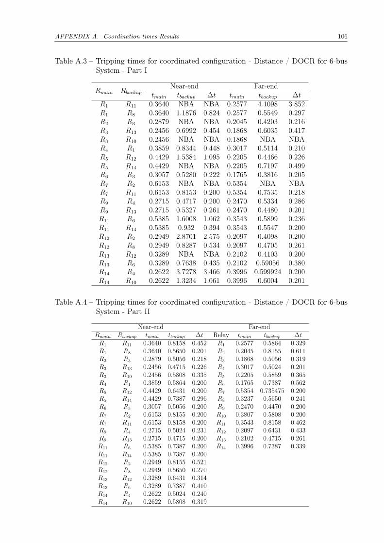
APPENDIX A. Coordination times Results 106
Table A.3 – Tripping times for coordinated configuration - Distance / DOCR for 6-busSystem - Part I
Rmain RbackupNear-end Far-end
tmain tbackup ∆t tmain tbackup ∆tR1 R11 0.3640 NBA NBA 0.2577 4.1098 3.852R1 R8 0.3640 1.1876 0.824 0.2577 0.5549 0.297R2 R3 0.2879 NBA NBA 0.2045 0.4203 0.216R3 R13 0.2456 0.6992 0.454 0.1868 0.6035 0.417R3 R10 0.2456 NBA NBA 0.1868 NBA NBAR4 R1 0.3859 0.8344 0.448 0.3017 0.5114 0.210R5 R12 0.4429 1.5384 1.095 0.2205 0.4466 0.226R5 R14 0.4429 NBA NBA 0.2205 0.7197 0.499R6 R3 0.3057 0.5280 0.222 0.1765 0.3816 0.205R7 R2 0.6153 NBA NBA 0.5354 NBA NBAR7 R11 0.6153 0.8153 0.200 0.5354 0.7535 0.218R9 R4 0.2715 0.4717 0.200 0.2470 0.5334 0.286R9 R13 0.2715 0.5327 0.261 0.2470 0.4480 0.201R11 R6 0.5385 1.6008 1.062 0.3543 0.5899 0.236R11 R14 0.5385 0.932 0.394 0.3543 0.5547 0.200R12 R2 0.2949 2.8701 2.575 0.2097 0.4098 0.200R12 R8 0.2949 0.8287 0.534 0.2097 0.4705 0.261R13 R12 0.3289 NBA NBA 0.2102 0.4103 0.200R13 R6 0.3289 0.7638 0.435 0.2102 0.59056 0.380R14 R4 0.2622 3.7278 3.466 0.3996 0.599924 0.200R14 R10 0.2622 1.3234 1.061 0.3996 0.6004 0.201
Table A.4 – Tripping times for coordinated configuration - Distance / DOCR for 6-busSystem - Part II
Near-end Far-endRmain Rbackup tmain tbackup ∆t Relay tmain tbackup ∆tR1 R11 0.3640 0.8158 0.452 R1 0.2577 0.5864 0.329R1 R8 0.3640 0.5650 0.201 R2 0.2045 0.8155 0.611R2 R3 0.2879 0.5056 0.218 R3 0.1868 0.5056 0.319R3 R13 0.2456 0.4715 0.226 R4 0.3017 0.5024 0.201R3 R10 0.2456 0.5808 0.335 R5 0.2205 0.5859 0.365R4 R1 0.3859 0.5864 0.200 R6 0.1765 0.7387 0.562R5 R12 0.4429 0.6431 0.200 R7 0.5354 0.735475 0.200R5 R14 0.4429 0.7387 0.296 R8 0.3237 0.5650 0.241R6 R3 0.3057 0.5056 0.200 R9 0.2470 0.4470 0.200R7 R2 0.6153 0.8155 0.200 R10 0.3807 0.5808 0.200R7 R11 0.6153 0.8158 0.200 R11 0.3543 0.8158 0.462R9 R4 0.2715 0.5024 0.231 R12 0.2097 0.6431 0.433R9 R13 0.2715 0.4715 0.200 R13 0.2102 0.4715 0.261R11 R6 0.5385 0.7387 0.200 R14 0.3996 0.7387 0.339R11 R14 0.5385 0.7387 0.200R12 R2 0.2949 0.8155 0.521R12 R8 0.2949 0.5650 0.270R13 R12 0.3289 0.6431 0.314R13 R6 0.3289 0.7387 0.410R14 R4 0.2622 0.5024 0.240R14 R10 0.2622 0.5808 0.319

APPENDIX A. Coordination times Results 107
Table A.5 – Tripping times for coordinated configuration (Hybrid) - Distance / DOCR for6-bus System - Part I
Rmain RbackupNear-end Far-end
tmain tbackup ∆t tmain tbackup ∆tR1 R11 0.5384 NBA NBA 0.3542 4.1116 3.757R1 R8 0.3667 1.1819 0.815 0.3233 0.5536 0.230R2 R3 0.2456 2.1845 1.939 0.1868 0.4203 0.234R3 R13 0.3289 0.6983 0.369 0.2101 0.6035 0.393R3 R10 0.4241 NBA NBA 0.3804 0.5841 0.204R4 R1 0.3641 0.8343 0.470 0.2578 0.5015 0.244R5 R12 0.2945 1.5511 1.257 0.2093 0.4465 0.237R5 R14 0.2622 NBA NBA 0.3996 0.7197 0.320R6 R3 0.3641 0.7168 0.353 0.2578 0.4956 0.238R7 R2 0.2456 0.4980 0.252 0.1868 0.3886 0.202R7 R11 0.2876 0.5584 0.271 0.2042 0.40601 0.202R9 R4 0.3857 0.5914 0.206 0.3015 0.5231 0.222R9 R13 0.3289 0.5327 0.204 0.2101 0.4470 0.237R11 R6 0.3056 1.6001 1.294 0.3543 0.5899 0.236R11 R14 0.2624 0.9322 0.670 0.3543 0.5547 0.200R12 R2 0.2876 2.8662 2.579 0.2097 0.4098 0.200R12 R8 0.3667 0.8258 0.459 0.2097 0.4705 0.261R13 R12 0.2945 NBA NBA 0.2102 0.4103 0.200R13 R6 0.3056 0.7655 0.460 0.2102 0.5905 0.380R14 R4 0.3857 3.7261 3.340 0.3896 0.5999 0.210R14 R10 0.4241 1.3201 0.896 0.3896 0.6004 0.211R8 NBA 0.6153 NBA NBA 0.5354 NBA NBAR10 NBA 0.2714 NBA NBA 0.2470 NBA NBA

APPENDIX A. Coordination times Results 108
Table A.6 – Tripping times for coordinated configuration (Hybrid) - Distance / DOCR for6-bus System - Part II
Near-end Far-endRmain Rbackup tmain tbackup ∆t Relay tmain tbackup ∆tR1 R11 0.5384 0.8016 0.263 R1 0.2578 0.5857 0.328R1 R8 0.3667 0.5715 0.205 R2 0.2042 0.8153 0.611R2 R3 0.24566 0.7354 0.490 R3 0.1868 0.7354 0.549R3 R13 0.3289 0.5715 0.243 R4 0.3015 0.7385 0.437R3 R10 0.4241 0.6281 0.204 R5 0.2204 0.4470 0.227R4 R1 0.3641 0.5864 0.222 R6 0.1765 0.5641 0.388R5 R12 0.2945 0.6431 0.349 R7 0.2876 0.6357 0.348R5 R14 0.2622 0.7387 0.476 R8 0.2833 0.4915 0.208R6 R3 0.3641 0.5656 0.202 R9 0.2470 0.6428 0.396R7 R2 0.2456 0.8155 0.570 R10 0.3804 0.7384 0.358R7 R11 0.2876 0.8158 0.528 R11 0.3012 0.5016 0.200R9 R4 0.3857 0.5924 0.207 R12 0.2093 0.5057 0.296R9 R13 0.3289 0.5715 0.243 R13 0.2101 0.8153 0.605R11 R6 0.3056 0.7387 0.433 R14 0.3896 0.5905 0.201R11 R14 0.2622 0.7387 0.476R12 R2 0.2876 0.8155 0.528R12 R8 0.3667 0.5850 0.218R13 R12 0.2945 0.6431 0.349R13 R6 0.3056 0.7387 0.433R14 R4 0.3857 0.5924 0.207R14 R10 0.4241 0.6239 0.200
A.2 System III: Eight Bus Network
A.2.1 DOCRs Only
Table A.7 – Tripping times for coordinated configuration - 8 Bus System
Rmain Rbackup tmain tbackup ∆tR1 R6 0.4184 0.7186 0.300R2 R1 0.8066 1.1062 0.300R2 R7 0.8066 1.1066 0.300R3 R2 0.7431 1.0433 0.300R4 R3 0.6460 0.9459 0.300R5 R4 0.5618 0.8617 0.300R6 R14 0.5181 0.9967 0.479R6 R5 0.5181 1.1376 0.620R7 R13 0.6966 0.9967 0.300R7 R5 0.6966 1.3994 0.703R8 R9 0.5209 1.1066 0.586R8 R7 0.5209 0.9782 0.457R9 R10 0.5683 0.8683 0.300R10 R11 0.6797 0.9797 0.300R11 R12 0.7565 1.0564 0.300R12 R14 0.8378 1.3994 0.562R12 R13 0.8378 1.1376 0.300R13 R8 0.4288 0.7288 0.300R14 R1 0.6780 1.1062 0.428R14 R9 0.6780 0.9782 0.300

APPENDIX A. Coordination times Results 109
Table A.8 – Tripping times for coordinated (Hybrid) configuration - 8 Bus System
Rmain Rbackup tmain tbackup ∆tR1 R6 0.5006 0.9539 0.453R2 R1 0.4075 1.0774 0.670R2 R7 0.4075 0.7075 0.300R3 R2 0.7774 1.0774 0.300R4 R3 0.5542 1.0774 0.523R5 R4 0.6539 0.9542 0.300R6 R14 0.6445 1.0774 0.433R6 R5 0.6445 0.9539 0.309R7 R13 0.5101 1.0972 0.587R7 R5 0.5101 1.0065 0.496R8 R9 0.4275 0.7295 0.302R8 R7 0.4275 1.0972 0.670R9 R10 0.7055 1.0065 0.301R10 R11 0.6469 1.0055 0.359R11 R12 0.7053 1.0069 0.302R12 R14 0.5980 1.0080 0.410R12 R13 0.5980 1.0053 0.407R13 R8 0.4978 0.7978 0.300R14 R1 0.7972 1.0972 0.300R14 R9 0.7972 1.0972 0.300
A.2.2 Distance and DOCRs
Table A.9 – Tripping times for coordinated configuration - Distance / DOCR for 8-busSystem
Rmain Rbackup tOCmain tOCbackup ∆t tZ2backup ∆t
R1 R6 0.4338 0.7372 0.303 0.7364 0.303R2 R1 0.8451 1.1468 0.302 1.2420 0.397R2 R7 0.8451 1.1496 0.305 1.1478 0.303R3 R2 0.7660 1.0660 0.300 1.0676 0.302R4 R3 0.6458 0.9515 0.306 0.9511 0.305R5 R4 0.5179 0.8320 0.314 0.8333 0.315R6 R14 0.5491 1.1688 0.620 1.1696 0.620R6 R5 0.5491 1.0471 0.498 1.0267 0.478R7 R13 0.7237 1.1720 0.448 1.1697 0.446R7 R5 0.7237 1.0471 0.323 1.0267 0.303R8 R9 0.5447 1.1496 0.605 1.0350 0.490R8 R7 0.5447 1.1496 0.605 1.1478 0.603R9 R10 0.6679 0.9764 0.309 0.9702 0.302R10 R11 0.7395 1.0480 0.308 1.0467 0.307R11 R12 0.7806 1.0946 0.314 1.0832 0.303R12 R14 0.8681 1.1688 0.301 1.1696 0.302R12 R13 0.8681 1.1720 0.304 1.1697 0.302R13 R8 0.4567 0.7620 0.305 0.7570 0.300R14 R1 0.7334 1.1468 0.413 1.2420 0.509R14 R9 0.7334 1.1496 0.416 1.0350 0.302
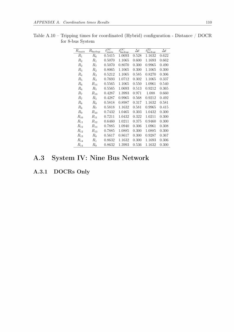
APPENDIX A. Coordination times Results 110
Table A.10 – Tripping times for coordinated (Hybrid) configuration - Distance / DOCRfor 8-bus System
Rmain Rbackup tOCmain tOCbackup ∆t tZ2backup ∆t
R1 R6 0.5415 1.0693 0.528 1.1632 0.622R2 R1 0.5070 1.1065 0.600 1.1693 0.662R2 R7 0.5070 0.8070 0.300 0.9965 0.490R3 R2 0.8065 1.1065 0.300 1.1065 0.300R4 R3 0.5212 1.1065 0.585 0.8270 0.306R5 R4 0.7693 1.0712 0.302 1.1065 0.337R6 R14 0.5565 1.1065 0.550 1.0961 0.540R6 R5 0.5565 1.0693 0.513 0.9212 0.365R7 R13 0.4287 1.3993 0.971 1.088 0.660R7 R5 0.4287 0.9965 0.568 0.9212 0.492R8 R9 0.5818 0.8987 0.317 1.1632 0.581R8 R7 0.5818 1.1632 0.581 0.9965 0.415R9 R10 0.7432 1.0465 0.303 1.0432 0.300R10 R11 0.7211 1.0432 0.322 1.0211 0.300R11 R12 0.6460 1.0211 0.375 0.9460 0.300R12 R14 0.7885 1.0940 0.306 1.0961 0.308R12 R13 0.7885 1.0885 0.300 1.0885 0.300R13 R8 0.5617 0.8617 0.300 0.9287 0.367R14 R1 0.8632 1.1632 0.300 1.1693 0.306R14 R9 0.8632 1.3993 0.536 1.1632 0.300
A.3 System IV: Nine Bus Network
A.3.1 DOCRs Only

APPENDIX A. Coordination times Results 111
Table A.11 – Tripping times for coordinated configuration - 9 Bus System
Rmain Rbackup tmain tbackup ∆tR1 R15 0.2001 0.4129 0.213R1 R17 0.2001 0.8567 0.657R2 R4 0.2002 0.9051 0.705R3 R1 0.1999 0.4512 0.251R4 R6 0.2000 0.5036 0.304R5 R3 0.2004 1.0736 0.873R6 R8 0.1999 0.9203 0.720R6 R23 0.1999 0.6885 0.489R7 R5 0.2001 1.3476 1.147R7 R23 0.2001 0.6885 0.488R8 R10 0.2003 0.4123 0.212R9 R7 0.2002 0.6767 0.477R10 R12 0.2001 4.9914 4.791R11 R9 0.2002 0.5026 0.302R12 R14 0.1999 0.5266 0.327R12 R21 0.1999 0.8247 0.625R13 R11 0.2002 0.5829 0.383R13 R21 0.2002 0.8247 0.624R14 R16 0.2001 2.7886 2.588R14 R19 0.2001 0.6922 0.492R15 R13 0.2001 0.5539 0.354R15 R19 0.2001 0.6922 0.492R16 R2 0.2002 0.5959 0.396R16 R17 0.2002 0.8567 0.657R17 R24 0.2001 NBA NBAR18 R2 0.2001 0.5959 0.396R18 R15 0.2001 0.4129 0.213R19 R24 0.2000 NBA NBAR20 R13 0.2001 0.5539 0.354R20 R16 0.2001 2.7886 2.588R21 R24 0.2000 NBA NBAR22 R11 0.2006 0.5829 0.382R22 R14 0.2006 0.5266 0.326R23 R22 0.2000 NBA NBAR24 R5 0.2000 1.3476 1.148R24 R8 0.2000 0.9203 0.720
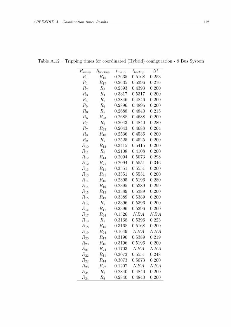
APPENDIX A. Coordination times Results 112
Table A.12 – Tripping times for coordinated (Hybrid) configuration - 9 Bus System
Rmain Rbackup tmain tbackup ∆tR1 R15 0.2635 0.5168 0.253R1 R17 0.2635 0.5396 0.276R2 R4 0.2393 0.4393 0.200R3 R1 0.3317 0.5317 0.200R4 R6 0.2846 0.4846 0.200R5 R3 0.2896 0.4896 0.200R6 R8 0.2688 0.4840 0.215R6 R23 0.2688 0.4688 0.200R7 R5 0.2043 0.4840 0.280R7 R23 0.2043 0.4688 0.264R8 R10 0.2536 0.4536 0.200R9 R7 0.2525 0.4525 0.200R10 R12 0.3415 0.5415 0.200R11 R9 0.2108 0.4108 0.200R12 R14 0.2094 0.5073 0.298R12 R21 0.2094 0.5551 0.346R13 R11 0.3551 0.5551 0.200R13 R21 0.3551 0.5551 0.200R14 R16 0.2395 0.5196 0.280R14 R19 0.2395 0.5389 0.299R15 R13 0.3389 0.5389 0.200R15 R19 0.3389 0.5389 0.200R16 R2 0.3396 0.5396 0.200R16 R17 0.3396 0.5396 0.200R17 R24 0.1526 NBA NBAR18 R2 0.3168 0.5396 0.223R18 R15 0.3168 0.5168 0.200R19 R24 0.1649 NBA NBAR20 R13 0.3196 0.5389 0.219R20 R16 0.3196 0.5196 0.200R21 R24 0.1703 NBA NBAR22 R11 0.3073 0.5551 0.248R22 R14 0.3073 0.5073 0.200R23 R22 0.1207 NBA NBAR24 R5 0.2840 0.4840 0.200R24 R8 0.2840 0.4840 0.200
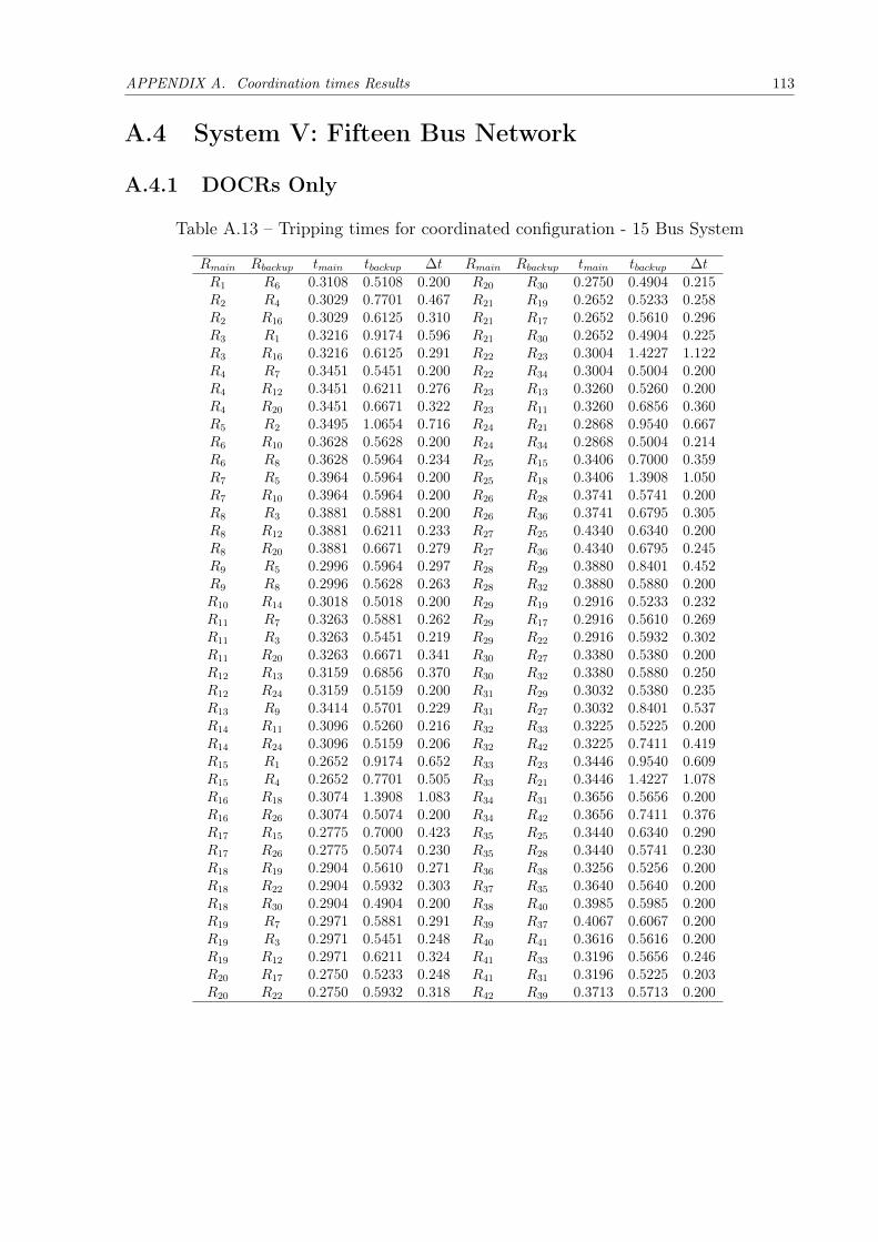
APPENDIX A. Coordination times Results 113
A.4 System V: Fifteen Bus Network
A.4.1 DOCRs Only
Table A.13 – Tripping times for coordinated configuration - 15 Bus System
Rmain Rbackup tmain tbackup ∆t Rmain Rbackup tmain tbackup ∆tR1 R6 0.3108 0.5108 0.200 R20 R30 0.2750 0.4904 0.215R2 R4 0.3029 0.7701 0.467 R21 R19 0.2652 0.5233 0.258R2 R16 0.3029 0.6125 0.310 R21 R17 0.2652 0.5610 0.296R3 R1 0.3216 0.9174 0.596 R21 R30 0.2652 0.4904 0.225R3 R16 0.3216 0.6125 0.291 R22 R23 0.3004 1.4227 1.122R4 R7 0.3451 0.5451 0.200 R22 R34 0.3004 0.5004 0.200R4 R12 0.3451 0.6211 0.276 R23 R13 0.3260 0.5260 0.200R4 R20 0.3451 0.6671 0.322 R23 R11 0.3260 0.6856 0.360R5 R2 0.3495 1.0654 0.716 R24 R21 0.2868 0.9540 0.667R6 R10 0.3628 0.5628 0.200 R24 R34 0.2868 0.5004 0.214R6 R8 0.3628 0.5964 0.234 R25 R15 0.3406 0.7000 0.359R7 R5 0.3964 0.5964 0.200 R25 R18 0.3406 1.3908 1.050R7 R10 0.3964 0.5964 0.200 R26 R28 0.3741 0.5741 0.200R8 R3 0.3881 0.5881 0.200 R26 R36 0.3741 0.6795 0.305R8 R12 0.3881 0.6211 0.233 R27 R25 0.4340 0.6340 0.200R8 R20 0.3881 0.6671 0.279 R27 R36 0.4340 0.6795 0.245R9 R5 0.2996 0.5964 0.297 R28 R29 0.3880 0.8401 0.452R9 R8 0.2996 0.5628 0.263 R28 R32 0.3880 0.5880 0.200R10 R14 0.3018 0.5018 0.200 R29 R19 0.2916 0.5233 0.232R11 R7 0.3263 0.5881 0.262 R29 R17 0.2916 0.5610 0.269R11 R3 0.3263 0.5451 0.219 R29 R22 0.2916 0.5932 0.302R11 R20 0.3263 0.6671 0.341 R30 R27 0.3380 0.5380 0.200R12 R13 0.3159 0.6856 0.370 R30 R32 0.3380 0.5880 0.250R12 R24 0.3159 0.5159 0.200 R31 R29 0.3032 0.5380 0.235R13 R9 0.3414 0.5701 0.229 R31 R27 0.3032 0.8401 0.537R14 R11 0.3096 0.5260 0.216 R32 R33 0.3225 0.5225 0.200R14 R24 0.3096 0.5159 0.206 R32 R42 0.3225 0.7411 0.419R15 R1 0.2652 0.9174 0.652 R33 R23 0.3446 0.9540 0.609R15 R4 0.2652 0.7701 0.505 R33 R21 0.3446 1.4227 1.078R16 R18 0.3074 1.3908 1.083 R34 R31 0.3656 0.5656 0.200R16 R26 0.3074 0.5074 0.200 R34 R42 0.3656 0.7411 0.376R17 R15 0.2775 0.7000 0.423 R35 R25 0.3440 0.6340 0.290R17 R26 0.2775 0.5074 0.230 R35 R28 0.3440 0.5741 0.230R18 R19 0.2904 0.5610 0.271 R36 R38 0.3256 0.5256 0.200R18 R22 0.2904 0.5932 0.303 R37 R35 0.3640 0.5640 0.200R18 R30 0.2904 0.4904 0.200 R38 R40 0.3985 0.5985 0.200R19 R7 0.2971 0.5881 0.291 R39 R37 0.4067 0.6067 0.200R19 R3 0.2971 0.5451 0.248 R40 R41 0.3616 0.5616 0.200R19 R12 0.2971 0.6211 0.324 R41 R33 0.3196 0.5656 0.246R20 R17 0.2750 0.5233 0.248 R41 R31 0.3196 0.5225 0.203R20 R22 0.2750 0.5932 0.318 R42 R39 0.3713 0.5713 0.200
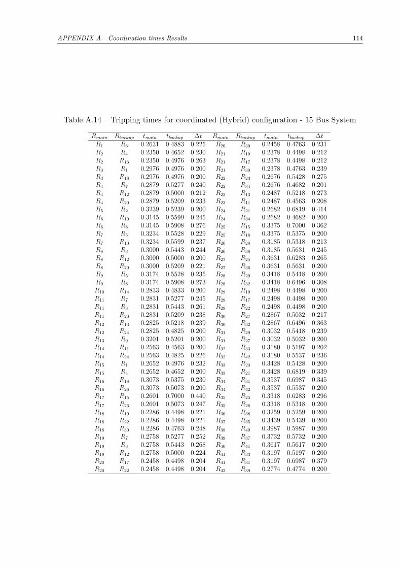
APPENDIX A. Coordination times Results 114
Table A.14 – Tripping times for coordinated (Hybrid) configuration - 15 Bus System
Rmain Rbackup tmain tbackup ∆t Rmain Rbackup tmain tbackup ∆tR1 R6 0.2631 0.4883 0.225 R20 R30 0.2458 0.4763 0.231R2 R4 0.2350 0.4652 0.230 R21 R19 0.2378 0.4498 0.212R2 R16 0.2350 0.4976 0.263 R21 R17 0.2378 0.4498 0.212R3 R1 0.2976 0.4976 0.200 R21 R30 0.2378 0.4763 0.239R3 R16 0.2976 0.4976 0.200 R22 R23 0.2676 0.5428 0.275R4 R7 0.2879 0.5277 0.240 R22 R34 0.2676 0.4682 0.201R4 R12 0.2879 0.5000 0.212 R23 R13 0.2487 0.5218 0.273R4 R20 0.2879 0.5209 0.233 R23 R11 0.2487 0.4563 0.208R5 R2 0.3239 0.5239 0.200 R24 R21 0.2682 0.6819 0.414R6 R10 0.3145 0.5599 0.245 R24 R34 0.2682 0.4682 0.200R6 R8 0.3145 0.5908 0.276 R25 R15 0.3375 0.7000 0.362R7 R5 0.3234 0.5528 0.229 R25 R18 0.3375 0.5375 0.200R7 R10 0.3234 0.5599 0.237 R26 R28 0.3185 0.5318 0.213R8 R3 0.3000 0.5443 0.244 R26 R36 0.3185 0.5631 0.245R8 R12 0.3000 0.5000 0.200 R27 R25 0.3631 0.6283 0.265R8 R20 0.3000 0.5209 0.221 R27 R36 0.3631 0.5631 0.200R9 R5 0.3174 0.5528 0.235 R28 R29 0.3418 0.5418 0.200R9 R8 0.3174 0.5908 0.273 R28 R32 0.3418 0.6496 0.308R10 R14 0.2833 0.4833 0.200 R29 R19 0.2498 0.4498 0.200R11 R7 0.2831 0.5277 0.245 R29 R17 0.2498 0.4498 0.200R11 R3 0.2831 0.5443 0.261 R29 R22 0.2498 0.4498 0.200R11 R20 0.2831 0.5209 0.238 R30 R27 0.2867 0.5032 0.217R12 R13 0.2825 0.5218 0.239 R30 R32 0.2867 0.6496 0.363R12 R24 0.2825 0.4825 0.200 R31 R29 0.3032 0.5418 0.239R13 R9 0.3201 0.5201 0.200 R31 R27 0.3032 0.5032 0.200R14 R11 0.2563 0.4563 0.200 R32 R33 0.3180 0.5197 0.202R14 R24 0.2563 0.4825 0.226 R32 R42 0.3180 0.5537 0.236R15 R1 0.2652 0.4976 0.232 R33 R23 0.3428 0.5428 0.200R15 R4 0.2652 0.4652 0.200 R33 R21 0.3428 0.6819 0.339R16 R18 0.3073 0.5375 0.230 R34 R31 0.3537 0.6987 0.345R16 R26 0.3073 0.5073 0.200 R34 R42 0.3537 0.5537 0.200R17 R15 0.2601 0.7000 0.440 R35 R25 0.3318 0.6283 0.296R17 R26 0.2601 0.5073 0.247 R35 R28 0.3318 0.5318 0.200R18 R19 0.2286 0.4498 0.221 R36 R38 0.3259 0.5259 0.200R18 R22 0.2286 0.4498 0.221 R37 R35 0.3439 0.5439 0.200R18 R30 0.2286 0.4763 0.248 R38 R40 0.3987 0.5987 0.200R19 R7 0.2758 0.5277 0.252 R39 R37 0.3732 0.5732 0.200R19 R3 0.2758 0.5443 0.268 R40 R41 0.3617 0.5617 0.200R19 R12 0.2758 0.5000 0.224 R41 R33 0.3197 0.5197 0.200R20 R17 0.2458 0.4498 0.204 R41 R31 0.3197 0.6987 0.379R20 R22 0.2458 0.4498 0.204 R42 R39 0.2774 0.4774 0.200