Concurrent Programming Actors, SALSA, Coordination Abstractions

Coordination of Concurrent One-to-Many Negotiations inMulti-Agent Systems
Khalid Mansour
Submitted in fulfilment of the requirementsfor the degree of Doctor of Philosophy
Faculty of Science, Engineering and TechnologySwinburne University of Technology
2014
to my parents
Abstract
Automated negotiation is a key interaction mechanism in distributed and multi-agentsystems. By adapting negotiation as an interaction method, autonomous agents caninteract, compete and cooperate with one another effectively. When the scale of ne-gotiation expands to involve more than two agents, the negotiation process becomesmore complex. This thesis addresses the problem of managing concurrent and de-pendent instances of automated negotiations in the one-to-many multi-agent systemswhere agents are self-interested, unwilling to disclose their private information (e.g.,utility structure, deadline, etc.) and the available information about the opponents ismainly the current history of their offers. In particular, this thesis considers the one-to-many negotiation where a buyer agent negotiates with multiple seller agents over oneor more objects concurrently. Dependent instances of negotiation occur when differentnegotiations are related and the situation of one instance affects the situation of one ormore other instances.
The main challenge of this thesis was to investigate the bidding strategy for a buyeragent negotiating concurrently with multiple seller agents over one or more negotiationobjects where each object can be characterized by one or more issues (attributes.) Mostof the current works in the literature target simple one-to-many negotiations whereagents negotiate a single negotiation issue. A few works investigate the case whereagents negotiate multiple issues. The work in this thesis proposes new negotiationtechniques to further improve the existing ones. In addition, more complicated ne-gotiation scenarios are investigated where agents negotiate over multiple objects withsingle or multiple negotiation issues.
The first step in the proposed solution approach is to analyze the one-to-many nego-tiations illustrating how different numbers of negotiation components can affect thecourse of the coordination mechanism in each negotiation scenario. In the context ofthis thesis, the negotiation components are: negotiation objects, negotiation issues andagents. Considering the different negotiation scenarios that can arise from the com-bination of different numbers of the negotiation components, appropriate mechanismsand algorithms are proposed to solve the relevant coordination problem in differentnegotiation scenarios. Defining different negotiation scenarios depend on the numberof negotiation objects, the number of negotiation issues per object and the number of

opponent agents per object. The number of each component can be either single ormultiple. Since the one-to-many negotiation is considered in this thesis, the number ofopponents is always multiple. Considering the behaviors of the opponent agents thatare still in negotiation, this thesis proposes effective coordination solutions that involvedetermining the value of the next counteroffer the buyer agent needs to propose to eachseller agent in each negotiation round.
Five one-to-many negotiation scenarios are recognized and named coordination sce-
narios. Coordinating the bidding strategy for a buyer agent in the five coordinationscenarios is the main focus of this thesis. This work advances the state of the art by an-alyzing different negotiation scenarios and proposing novel mechanisms that improveand further extend the existing work to solve more complex negotiation scenarios.
The main approach adopted in solving the coordination problems in the one-to-manynegotiation is to change the negotiation strategy during negotiation (i.e., in real-time)in response to the current behaviors of the opponents in terms of their concessions. Forexample, the convexity of a concession curve is one of the parameters of a negotiationstrategy. If the convexity of a concession curve can be dynamically controlled dur-ing negotiation, then a particular coordination problem can be solved. Since differentcoordination scenarios have different numbers of components and related variables,then different coordination mechanisms are necessary to deal with different coordina-tion scenarios. For example, when an agent negotiates with multiple other agents overone object characterized by one issue (e.g., price), then the agent can use a coordina-tion mechanism that manages the convexity of its concession curve(s) to maximize itsutility. In this case, the agent cannot consider other cooperative solutions such as thetrade-off mechanism.
Experiments that compare between the proposed negotiation strategies and the state-of-the-art strategies are used to test the effectiveness and robustness of the proposedsolutions empirically. The main performance criteria in the experiments are the agree-ment rate and the utility rate. In most cases, the results of the experiments prove thatthe proposed solutions to the coordination problems in different coordination scenar-ios are effective and robust in terms of both, the utility rates and the agreement rates.In scenarios where there is room for cooperation e.g., in case of multi-issue negotia-tion, the proposed techniques consider also the social welfare and the fairness of anagreement as performance criteria.
iii

Acknowledgements
I express my deepest gratitude and appreciation to my supervisor and mentor ProfessorRyszard Kowalczyk for providing me with the opportunity to do a PhD. ProfessorKowalczyk offered me help and guidance throughout my study journey. Our regularmeetings and discussions ignited many research ideas which I investigated further.To me, Professor Kowalczyk is a supervisor and a friend. He always supported andencouraged me during tough times.
Special thanks goes to the current and former members of the Intelligent Agent Tech-nology group, especially my associate supervisor Dr. Bao Vo. The IAT group memberswere helpful and supportive throughout my candidature.
I would also like to thank Swinburne University of Technology for offering me a fullscholarship and all the needed resources to complete my study including tuition fees,stipends, access to abundant research materials and funds to attend conferences insideand outside Australia. Special thanks goes to the Faculty of Information and Commu-nication Technologies for being the host of my research work.
I would also like to thank my friends at the SUCCESS research center whom I spentgood times with. My friends who were very helpful and supportive all the way duringmy candidature.
Most importantly, I would like to thank my wife Lama for her patience and supportand my children Lujain, Walid and Jena who sacrificed a lot of playing time with meduring my study.
Declaration
This thesis contains no material which has been accepted for the award of any otherdegree or diploma, except where due reference is made. To the best of my knowledge,this thesis contains no material previously published or written by another person ex-cept where due reference is made in the text of the thesis.
Khalid Mansour
29/01/2014
Publications
Parts of the material presented in this thesis have previously appeared in most of thefollowing publications:
1. K. Mansour and R. Kowalczyk. An Approach to One-to-Many Concurrent Ne-gotiation. Group Decision and Negotiation. (Accepted for publication on 27/01/2014).Impact factor: 0.897
2. K. Mansour and R. Kowalczyk. An Approach for Coordinating the BiddingStrategy in Multi-Issue Multi-Object Negotiation with Multiple Providers. IEEE
Transactions on Systems, Man, and Cybernetics, Part B. (First revision was sub-mitted on 09/09/2013). Impact factor: 3.236
3. K. Mansour, R. Kowalczyk, and M. Wosko. Aspects of Coordinating the BiddingStrategy in Concurrent One-to-Many Negotiation. In Knowledge Engineering
and Management, 103-115, 2014, Springer.
4. K. Mansour and R. Kowalczyk. On Dynamic Negotiation Strategy for Concur-rent Negotiation over Distinct Objects. In Marsa-Maestre, I.; Lopez-Carmona,M.A.; Ito, T.; Zhang, M.; Bai, Q.; Fujita, K. (Eds.). Novel Insights in Agent-
based Complex Automated Negotiation, Vol 535, 2014, Springer.
5. M. Wosko, I. Moser, and K. Mansour. Scheduling for Optimal Response Timesin Queues of Stochastic Workflows. Lecture Notes in Computer Science, 8272:502-513, 2013, Springer.
6. K. Mansour and R. Kowalczyk. On Dynamic Negotiation Strategy for Con-current Negotiation over Distinct Objects. The 5th International Workshop on
Agent-Based Complex Automated Negotiations (ACAN) at AAMAS, 65-72, 2012.
7. K. Mansour. Managing Concurrent Negotiations in Multi-agent Systems. Lec-
ture Notes in Artificial Intelligence, 7310:380-383, 2012, Springer.
8. K. Mansour, R. Kowalczyk, and M. B. Chhetri. On Effective Quality of ServiceNegotiation. In the 12th IEEE/ACM International Symposium on Cluster, Cloud
and Grid Computing, 684-685, 2012.
9. K. Mansour, R. Kowalczyk, and M. Wosko. Concurrent Negotiation over Qual-ity of Service. In the Proc. of the IEEE Ninth International Conference on
Services Computing, 446-453, 2012.
10. K. Mansour and R. Kowalczyk. A Meta-Strategy for Coordinating of One-to-Many Negotiation over Multiple Issues. In Y. Wang and T. Li, editors. Founda-
tions of Intelligent Systems, 343-353, 2011, Springer.
11. K. Mansour, R. Kowalczyk, and B. Q. Vo. Real-Time Coordination of Concur-rent Multiple Bilateral Negotiations under Time Constraints. Lecture Notes in
Artificial Intelligence, 6464:385-394, 2010, Springer.
vii

Contents
Abstract ii
Acknowledgements iv
Declaration v
Publications vi
1 Introduction 11.1 Problem Description . . . . . . . . . . . . . . . . . . . . . . . . . . 4
1.2 Usage Scenarios . . . . . . . . . . . . . . . . . . . . . . . . . . . . . 5
1.2.1 Scientific Workflow in the Cloud Scenario . . . . . . . . . . . 5
1.2.2 Holiday Booking Scenario . . . . . . . . . . . . . . . . . . . 8
1.2.3 Supply Chain Scenario . . . . . . . . . . . . . . . . . . . . . 9
1.3 Research Questions . . . . . . . . . . . . . . . . . . . . . . . . . . . 10
1.4 Contributions . . . . . . . . . . . . . . . . . . . . . . . . . . . . . . 12
1.5 Thesis Outline . . . . . . . . . . . . . . . . . . . . . . . . . . . . . . 14
2 Background and Related Work 172.1 Multiagent Systems Paradigm . . . . . . . . . . . . . . . . . . . . . 17
2.2 Automated Negotiation . . . . . . . . . . . . . . . . . . . . . . . . . 20
2.3 Approaches to Negotiation . . . . . . . . . . . . . . . . . . . . . . . 27
2.3.1 Game Theory-Based Approaches . . . . . . . . . . . . . . . 28
2.3.2 Learning and Reasoning Based Approaches . . . . . . . . . . 32
2.3.3 Heuristic-Based Tactics . . . . . . . . . . . . . . . . . . . . 40
2.3.3.1 Time-Dependent Tactics . . . . . . . . . . . . . . . 41

Contents
2.3.3.2 Resource-Dependent Tactics . . . . . . . . . . . . 43
2.3.3.3 Behavior-Dependent Tactics . . . . . . . . . . . . . 44
2.3.3.4 Mixing of Tactics . . . . . . . . . . . . . . . . . . 46
2.3.3.5 Trade-off Generation Approach . . . . . . . . . . . 48
2.3.4 Argumentation-Based Negotiation . . . . . . . . . . . . . . . 53
2.4 Dependencies and Coordination . . . . . . . . . . . . . . . . . . . . 55
2.4.1 Interdependency Amongst Objects . . . . . . . . . . . . . . . 57
2.4.2 Interdependency Amongst Issues . . . . . . . . . . . . . . . 59
2.5 Coordination and Negotiation . . . . . . . . . . . . . . . . . . . . . . 60
2.5.1 One-to-Many Negotiation Over a Single Issue . . . . . . . . . 65
2.5.2 One-to-Many Negotiation Over Multiple Issues . . . . . . . . 71
2.5.3 One-to-Many Negotiation Over Multiple Distinct Objects . . 75
2.6 Summary . . . . . . . . . . . . . . . . . . . . . . . . . . . . . . . . 80
3 General Negotiation Model 833.1 Introduction . . . . . . . . . . . . . . . . . . . . . . . . . . . . . . . 83
3.2 Overview of the Negotiation Model . . . . . . . . . . . . . . . . . . 84
3.2.1 Negotiation Model . . . . . . . . . . . . . . . . . . . . . . . 84
3.2.2 Evaluation Decisions . . . . . . . . . . . . . . . . . . . . . . 90
3.3 Summary . . . . . . . . . . . . . . . . . . . . . . . . . . . . . . . . 93
4 Coordination Scenarios and Solution Approach 954.1 Coordination Problem in One-to-Many Negotiation . . . . . . . . . . 95
4.2 Coordination Scenarios . . . . . . . . . . . . . . . . . . . . . . . . . 99
4.3 Solution Approach . . . . . . . . . . . . . . . . . . . . . . . . . . . 103
4.4 Global and Local Reservation Values . . . . . . . . . . . . . . . . . . 109
4.5 General Experimental Settings . . . . . . . . . . . . . . . . . . . . . 110
4.5.1 Simulation Environment . . . . . . . . . . . . . . . . . . . . 111
4.5.2 Experimental Settings . . . . . . . . . . . . . . . . . . . . . 112
4.6 Summary . . . . . . . . . . . . . . . . . . . . . . . . . . . . . . . . 116
5 A Single Negotiation Issue for One or Multiple Objects 1185.1 Introduction . . . . . . . . . . . . . . . . . . . . . . . . . . . . . . . 118
5.2 SSM Coordination Scenario . . . . . . . . . . . . . . . . . . . . . . 120
ix
Contents
5.2.1 Managing the Convexity Parameter . . . . . . . . . . . . . . 121
5.2.2 Experimental Results and Discussion . . . . . . . . . . . . . 125
5.2.2.1 Testing under Different Deadline Lengths . . . . . 127
5.2.2.2 Testing Under Different Reservation Interval Overlaps130
5.2.2.3 Testing under Other Negotiation Environmental Con-ditions . . . . . . . . . . . . . . . . . . . . . . . . 131
5.2.3 Testing Different Strategy Metrics . . . . . . . . . . . . . . . 134
5.3 MSM Coordination Scenario . . . . . . . . . . . . . . . . . . . . . . 137
5.3.1 Global MSM Strategy . . . . . . . . . . . . . . . . . . . . . 139
5.3.1.1 Experimental Results and Discussions . . . . . . . 142
5.3.2 Local and Hybrid MSM Strategies . . . . . . . . . . . . . . . 146
5.3.2.1 Experimental Results and Discussion . . . . . . . . 148
5.4 Summary . . . . . . . . . . . . . . . . . . . . . . . . . . . . . . . . 153
6 A Single Object with Multiple Negotiation Issues 1556.1 Introduction . . . . . . . . . . . . . . . . . . . . . . . . . . . . . . . 155
6.2 Iterative Offer Generation Tactics . . . . . . . . . . . . . . . . . . . . 158
6.3 The Meta-Strategy Model . . . . . . . . . . . . . . . . . . . . . . . . 163
6.4 Experimental Evaluation . . . . . . . . . . . . . . . . . . . . . . . . 167
6.4.1 Experimental Settings . . . . . . . . . . . . . . . . . . . . . 167
6.4.2 Experimental Results and Discussion . . . . . . . . . . . . . 169
6.4.2.1 Testing under Different Deadline Lengths . . . . . 169
6.4.2.2 Testing under Different Agreement Zone Lengths . 179
6.4.2.3 Testing Against Mixed-Tactics Dependent Seller Agents185
6.4.2.4 Testing the IOG-conceder Agent . . . . . . . . . . 189
6.5 Summary . . . . . . . . . . . . . . . . . . . . . . . . . . . . . . . . 194
7 Multiple Objects with Multiple Negotiation Issues 1977.1 Introduction . . . . . . . . . . . . . . . . . . . . . . . . . . . . . . . 197
7.2 MMS Coordination Approach . . . . . . . . . . . . . . . . . . . . . 199
7.2.1 Experimental Results and Discussion . . . . . . . . . . . . . 203
7.2.1.1 Negotiation Deadline . . . . . . . . . . . . . . . . 205
7.2.1.2 Convexity of the Concession Curve . . . . . . . . . 208
7.3 MMM Coordination approach . . . . . . . . . . . . . . . . . . . . . 210
x

Contents
7.3.1 Experimental Results and Discussion . . . . . . . . . . . . . 212
7.3.1.1 Negotiation Deadline . . . . . . . . . . . . . . . . 213
7.3.1.2 Convexity of the Concession Curve . . . . . . . . . 215
7.3.1.3 Number of the Seller Agents per Object . . . . . . 217
7.3.1.4 Length of the Agreement Zone . . . . . . . . . . . 219
7.4 Summary . . . . . . . . . . . . . . . . . . . . . . . . . . . . . . . . 221
8 Conclusion 2238.1 Answers to the Research Questions . . . . . . . . . . . . . . . . . . . 228
8.2 Directions for Future Work . . . . . . . . . . . . . . . . . . . . . . . 231
Bibliography 234
xi

List of Figures
1.1 Data set generation workflow . . . . . . . . . . . . . . . . . . . . . . 6
1.2 Resources on the cloud . . . . . . . . . . . . . . . . . . . . . . . . . 7
1.3 Travel booking scenario . . . . . . . . . . . . . . . . . . . . . . . . 8
1.4 Supply chain . . . . . . . . . . . . . . . . . . . . . . . . . . . . . . . 9
2.1 Agent-based electronic market structures . . . . . . . . . . . . . . . . 20
2.2 Taxonomy of game theory . . . . . . . . . . . . . . . . . . . . . . . . 29
2.3 AI Learning & reasoning methods used in automated negotiation . . . 32
2.4 Polynomial (left), exponential (middle) and sigmoid decision functioncurvatures using different β values . . . . . . . . . . . . . . . . . . . 42
2.5 The outcome space for two agents negotiating over a single negotiationissue (left) and multiple negotiation issues. . . . . . . . . . . . . . . . 49
2.6 Iso-curves . . . . . . . . . . . . . . . . . . . . . . . . . . . . . . . . 51
2.7 Common dependency types . . . . . . . . . . . . . . . . . . . . . . . 56
2.8 Categorization of coordination in multiagent systems . . . . . . . . . 61
3.1 Complex one-to-many negotiation . . . . . . . . . . . . . . . . . . . 85
3.2 One-to-many negotiation . . . . . . . . . . . . . . . . . . . . . . . . 86
3.3 The decision process of accepting a multi-issue offer . . . . . . . . . 93
4.1 Negotiation scenarios . . . . . . . . . . . . . . . . . . . . . . . . . . 99
4.2 A snapshot of the experimental working environment . . . . . . . . . 111
5.1 One-to-many negotiation over a single object of a single issue . . . . 120
5.2 The effect of different β values on the concession curve . . . . . . . . 122
5.3 The effect of equal and shorter deadlines on the performance of differ-ent bidding strategies. . . . . . . . . . . . . . . . . . . . . . . . . . . 127

List of Figures
5.4 The effect of longer deadlines and randomly selected deadlines on theperformance of different bidding strategies. . . . . . . . . . . . . . . 129
5.5 The effect of different overlap percentages on the performance of dif-ferent bidding strategies. . . . . . . . . . . . . . . . . . . . . . . . . 131
5.6 The effect of selecting random deadlines and random overlaps on theperformance of different bidding strategies when agents must honortheir agreements. . . . . . . . . . . . . . . . . . . . . . . . . . . . . 132
5.7 Seller agents mix between the time-dependent and the behavior-dependenttactics where all agents need to honor their agreements. . . . . . . . . 133
5.8 Seller agents mix between the time-dependent and the behavior-dependenttactics to generate their offers given that all agents must honor theiragreements. . . . . . . . . . . . . . . . . . . . . . . . . . . . . . . . 135
5.9 Seller agents who use the time-dependent and the MTD tactics to gen-erate their offers given that all agents must honor their agreements. . 136
5.10 One-to-many negotiation over multiple negotiation objects of one issue 138
5.11 Testing the strategies GMSM, SR and GS; number of seller agents varies143
5.12 Testing the strategies GMSM, SR and GS; number of seller agents varies144
5.13 Testing the strategies GMSM, SR and GS; number of objects varies . . 144
5.14 Testing the strategies GMSM, SR and GS; the seller agents mix be-tween the time-dependent tactics and the behavior dependent tacticsto generate their offers . . . . . . . . . . . . . . . . . . . . . . . . . 145
5.15 Testing the strategies LMSM, SR and GS; number of seller agents varies 148
5.16 Testing the strategies LMSM, SR and GS; number of objects varies . . 149
5.17 Testing the strategies GMSM, SR and GS; the seller agents mix be-tween the time-dependent tactics and the behavior dependent tactic togenerate their offers . . . . . . . . . . . . . . . . . . . . . . . . . . . 150
5.18 Testing the strategies HMSM, SR and GS; number of seller agents varies151
5.19 Testing HMSM, SR and GS; number of objects varies . . . . . . . . . 151
5.20 Testing GMSM, LMSM and HMSM; number of seller agents varies . . 152
5.21 Testing HMSM, SR and GS. The seller agents mix between the time-dependent tactics and the behavior dependent tactic to generate theiroffers . . . . . . . . . . . . . . . . . . . . . . . . . . . . . . . . . . 153
6.1 One object with multiple negotiation issues . . . . . . . . . . . . . . 157
6.2 Illustration of the IOG-trade-off mechanism . . . . . . . . . . . . . . 159
6.3 The buyer agents have shorter deadlines than the seller agents’ dead-lines and the number of seller agents per object varies. . . . . . . . . 171
xiii
List of Figures
6.4 The buyer agents have shorter deadlines than the seller agents’ dead-lines and the number of seller agents per object varies. . . . . . . . . 173
6.5 The buyer agents have shorter deadlines than the seller agents’ dead-lines and the number of issues per object varies. . . . . . . . . . . . . 174
6.6 The buyer agents have longer deadlines than the seller agents’ dead-lines and the number of seller agents per object varies. . . . . . . . . 176
6.7 The buyer agents have longer deadlines than the seller agents’ dead-lines and the number of issues per object varies. . . . . . . . . . . . . 177
6.8 All agents have the same deadline and the number of seller agents perobject varies. . . . . . . . . . . . . . . . . . . . . . . . . . . . . . . 178
6.9 All agents have the same deadline and the number of issues per objectvaries. . . . . . . . . . . . . . . . . . . . . . . . . . . . . . . . . . . 179
6.10 Agents have small overlap between their reservation intervals and thenumber of seller agents per object varies. . . . . . . . . . . . . . . . 181
6.11 Agents have small overlap between their reservation intervals and thenumber of issues per object varies. . . . . . . . . . . . . . . . . . . . 182
6.12 Agents have large overlap between their reservation intervals and thenumber of seller agents per object varies. . . . . . . . . . . . . . . . 183
6.13 Agents have large overlap between their reservation intervals and thenumber of issues per object varies. . . . . . . . . . . . . . . . . . . . 184
6.14 The number of seller agents per objects is larger than the number ofissues per object. . . . . . . . . . . . . . . . . . . . . . . . . . . . . 186
6.15 The number of seller agents per objects is smaller than the number ofissues per object. . . . . . . . . . . . . . . . . . . . . . . . . . . . . 188
6.16 The number of seller agents per object varies. . . . . . . . . . . . . . 190
6.17 The number of issues per object varies. . . . . . . . . . . . . . . . . . 192
6.18 The number of seller agents per object varies. . . . . . . . . . . . . . 193
6.19 The number of issues per object varies. . . . . . . . . . . . . . . . . . 194
7.1 One-to-many negotiation over multiple object with multiple issues . . 198
7.2 Complex one-to-many negotiation . . . . . . . . . . . . . . . . . . . 199
7.3 The effect of different deadlines on the utility rate and the agreement rate206
7.4 The effect of different deadlines on the Nash product rate and the utilitydifference rate . . . . . . . . . . . . . . . . . . . . . . . . . . . . . . 207
7.5 The effect of curve convexities on the utility rate and the agreement rate 209
7.6 The effect of curve convexities on the Nash product rate and the utilitydifference rate . . . . . . . . . . . . . . . . . . . . . . . . . . . . . . 210
xiv

List of Figures
7.7 The effect of different deadlines on the utility rate and the agreement rate213
7.8 The effect of different deadlines on the Nash product rate and the utilitydifference rate . . . . . . . . . . . . . . . . . . . . . . . . . . . . . . 214
7.9 The effect of different buyers’ β values on the utility rate and the agree-ment rate . . . . . . . . . . . . . . . . . . . . . . . . . . . . . . . . 215
7.10 The effect of different buyers’ β values on the utility rate and the agree-ment rate . . . . . . . . . . . . . . . . . . . . . . . . . . . . . . . . 216
7.11 The effect of different number of sellers on the utility rate and theagreement rate . . . . . . . . . . . . . . . . . . . . . . . . . . . . . 217
7.12 The effect of different number of sellers on the Nash product rate andthe utility difference . . . . . . . . . . . . . . . . . . . . . . . . . . . 218
7.13 The effect of different agreement zone lengths on the utility rate andthe agreement rate . . . . . . . . . . . . . . . . . . . . . . . . . . . 220
7.14 The effect of different agreement zone lengths on the Nash product rateand the utility difference rate . . . . . . . . . . . . . . . . . . . . . . 221
xv

List of Tables
4.1 Example of three negotiation rounds . . . . . . . . . . . . . . . . . . 106
4.2 Negotiation tactics, their parameters and weights for possible mixingbetween different tactics . . . . . . . . . . . . . . . . . . . . . . . . 112
5.1 Different βC strategy variants . . . . . . . . . . . . . . . . . . . . . 134
6.1 Example of exchanged offers over two negotiation issues . . . . . . . 160
6.2 Experimental settings of different deadline lengths . . . . . . . . . . . 170
6.3 Experimental settings of different agreement zone lengths . . . . . . . 180
6.4 Experimental settings . . . . . . . . . . . . . . . . . . . . . . . . . . 189
7.1 Local reservation value weights (IW) . . . . . . . . . . . . . . . . . 199
7.2 Local reservation values (LR) . . . . . . . . . . . . . . . . . . . . . 199
Chapter 1
Introduction
Negotiation is prevalent in our daily life as a method of conflict resolution. Negotiation
is a major mechanism of interaction and decision making in many important domains
such as politics, law, sociology, business and personal situations (e.g., [75][64][130]).
In particular, negotiation can be looked at as a process of distributed decision making
amongst two or more parties who seek to agree upon a conflicting matter [61]. The ne-
gotiation theory has been investigated from different perspectives such as game theory
[47] and decision-analytic approach [116].
The tremendous advances in the web technology and networking have opened a new
era for the application of automated negotiation where software agents or autonomous
computer systems are able to automate some aspects of the negotiation process. Au-
tomated negotiation has been an active research area for more than a decade (e.g.,
[2][32][33][39]). As negotiation is an effective mechanism for decision making and
conflict resolution, the automation process of negotiation aims for better negotiation
results in terms of utility gain, agreement rate, social welfare and fairness. In addition,
the automation of the negotiation process aims to enable software agents to work on
behalf of the users to reach agreements quickly with the best possible outcome. More-
over, the automation of negotiation enables agents to negotiate complex contracts more
efficiently than humans do. Complex contracts may contain a large number of issues
that can be either interdependent or independent.
Negotiation is one of the coordination approaches that can be used to coordinate var-
ious activities amongst different parties such as scheduling and resource allocation
(e.g., [153] [55]). However, the main focus of this thesis is the problem of coordinat-
Chapter 1. Introduction
ing the bidding strategy for a buyer agent conducting multiple negotiations simulta-
neously. The multiple concurrent negotiations are assumed to be interdependent since
all negotiations share a common goal(s) and a common resource(s). The resources are
managed in a way to achieve the common goal(s). For example, if the common goal is
to reach an agreement with a high utility then the resources (e.g., money) are dynam-
ically allocated during negotiation amongst the multiple negotiations to help achieve
the specified goal.
Even though the proposed negotiation model, the proposed coordination mechanisms
and the experimental results present a buyer agent’s point view, the negotiation model
is general and can present a seller agents’ point of view as well. In addition, the
proposed coordination mechanisms can still be used by a seller agent. However, the
seller agent might also consider other factors when using the proposed mechanisms,
such as reputation.
A few existing works in the literature address the aspects of the coordination problem
in the one-to-many negotiation. However, most of the related works focus on simple
negotiation scenarios where agents aim to negotiate a single issue. In addressing the
problem, we use the divide and conquer strategy to tackle it systematically through
different scenarios. The cardinalities of negotiation objects, negotiation issues per
object and providers/opponents per object are considered the main negotiation criteria
and are used to define different negotiation scenarios. For example if the cardinality
for the set of agents is 2, then the negotiation is of a bilateral type.
A subset of the negotiation scenarios is highlighted and named coordination scenar-
ios. It encompasses all the one-to-many negotiation variants that are determined by
the negotiation components mentioned in the previous paragraph. Each coordination
scenario is characterized by a unique combination of a number of distinct objects, a
number of issues per object and a number of providers per object. For example, if a
buyer agent seeks to procure a storage space, a software application and a certain com-
putational power from the cloud, given that all specifications are agreed upon apart
from the price, then the buyer agent needs to negotiate the price of each service with
one or more providers. This scenario is characterized by multiple negotiation objects
(e.g., storage space) given that each object has one negotiation issue (e.g., price) and
multiple providers. If the number of negotiation issues per object is multiple, then a
different coordination scenario arises.
2
For each different coordination scenario, one or more negotiation parameters are se-
lected to be controlled or adapted during negotiation. The adaptation of a certain ne-
gotiation parameter reflects the behaviors of the current opponents in terms of their
concessions in the current negotiation encounter. For example, the convexity of the
concession curve is one of the parameters that can be managed during negotiation. To
validate the proposed solutions, experiments are designed and implemented to compare
between the performance of the proposed solutions and other benchmark solutions in
terms of the utility rates, agreement rates, social welfare etc.
The bilateral negotiation is the basic form of negotiation where two agents exchange
offers and counteroffers. Different game theoretic and artificial intelligence (AI) mech-
anisms have been proposed in the process of decision making during negotiation (e.g.,
[13] [12] [163] [6]). However, it is difficult to apply the game theoretic approaches in
real negotiations since they typically require that the two negotiation partners disclose
their preference profiles which is an unrealistic assumption due to privacy and trust
issues. In most cases, the AI mechanisms are heuristic approaches that require either
historical data or use learning mechanisms that need considerable computational power
and time. When it comes to making a decision in the one-to-many negotiation, the sit-
uation becomes even more complicated since there are multiple interactions between
multiple agents.
The mediated negotiation is a negotiation approach where two or more agents nego-
tiate using a mediator (e.g., [79][31]). The approach requires that agents send their
proposals to the mediator. The participating agents need also to disclose all or some of
their preference profiles to the mediator. The mediator uses the collection of profiles
and attempts at finalizing an agreement that is fair and acceptable for all parties. The
trust and privacy matters are the main obstacles in adopting the mediated negotiation
approach.
The proposed mechanisms in this thesis do not require historical data. As a source
of information, they rely only on the offers received from the opponents during the
current negotiation. Finally, the negotiation strategy components that are considered
in this thesis are: the reservation value and the set of negotiation tactics with their
parameters. A dynamic negotiation strategy may change the value of any of these
parameters during negotiation to accommodate a new negotiation situation.
3
Chapter 1. Introduction
1.1 Problem Description
When a software agent interacts with other software agents through negotiations, it
needs to decide the values of the proposals in every negotiation round. In other words,
the agent needs to have a bidding strategy that enables it from taking appropriate deci-
sions regarding the values of the proposals in every negotiation round.
This research aims at advancing the state-of-the-art in the process of automation of ne-
gotiation and particularly it focuses on the problem of coordinating the bidding strategy
for multiple concurrent one-to-many negotiations in multi-agent systems. The bidding
strategy controls the process of generating offers and counteroffers. The bidding strat-
egy and negotiation strategy are used interchangeably in this thesis. A negotiating
agent needs to coordinate its concurrent multiple negotiations when interacting with
multiple agents to improve one or more performance criteria. The key point in solving
any coordination problem is the ability to manage dependencies between related ac-
tivities [84]. In other words, the dependencies between the different related activities
cause the coordination problem. The activities of an agent in the negotiation context
mean all possible actions that can be taken by an agent as defined by a negotiation
protocol. For example, proposing an offer with a certain value and accepting an agree-
ment are examples of possible actions during negotiation. Given that a negotiation
strategy consists of a set of parameters with certain values, the coordination problem
is to define a value for each parameters dynamically during negotiation.
The proposed coordination mechanisms (decision making mechanisms) depend on the
behaviors of the current opponents in terms of their concessions. The concessions of
the negotiating agents affect the coordination mechanisms that decide the proposal val-
ues in the next negotiation round. Taking into consideration the concessions offered
by the negotiating agents in the previous negotiation round(s), one or more negotia-
tion parameters can be changed by the coordination mechanisms. The convexity of
the concession curve is one of the negotiation strategy parameters than can be ma-
nipulated during negotiation. Chapter 4 contains more details about the coordination
problem and the solution approach.
4
1.2. Usage Scenarios
1.2 Usage Scenarios
This work mainly investigates the bidding strategy problem in one-to-many automated
negotiation. Ma and Leung in their book titled ‘Bidding Strategies in Agent-Based
Continuous Double Auctions’ wrote [82]:
Automation of bidding is complex. Given the variety of auction pro-
tocols, it is perhaps not surprising that the bidding strategies of the par-
ticipants cover a similarly broad spectrum of behaviors. In short, there is
no optimal strategy that can be used in all cases. To be effective, bidding
strategies need to be tailored to the type of the auction in which they are to
be used. Perhaps the key challenges in this area is to design effective and
efficient strategies that agents can use to guide their bidding behavior.
Deciding on a bidding strategy in the one-to-many negotiation is a nontrivial problem
since an agent needs to analyze the behaviors of the opponents and reply to each one of
them and/or to each group of them differently. It is even more complex than the bidding
strategy in auctions since the auctions assume bidding on one issue (mainly price) in
most cases. The one-to-many negotiation applies to many real life interaction scenar-
ios. The electronic commerce is a potential application domain for the agent-mediated
with fully automated negotiation [132]. To motivate this research, three potential appli-
cation scenarios are presented. The first one shows how the one-to-many negotiation
can reduce cost and/or improve the efficiency of the scientific workflows execution.
The second one presents the holiday booking scenario and how the one-to-many nego-
tiation helps travelers find good deals while the third application scenario shows how
automated negotiation can help in the process of supply chain management.
1.2.1 Scientific Workflow in the Cloud Scenario
Many scientific applications nowadays are highly demanding for both computational
and storage resources [152][26]. For example, the astrophysics applications process
large amounts of data such as pulsar searching which is a scientific application that
processes terabytes of data [26]. The pulsar searching has a workflow of processing
the raw data collected from the telescope and preparing it for decision making. Such
5
Chapter 1. Introduction
scientific workflows produce large amount of intermediate datasets and require inten-
sive computational power. The generated intermediate datasets are needed either for
generating of other intermediate datasets or for analysis. The intermediate datasets are
interdependent since an intermediate dataset requires one or more other datasets for its
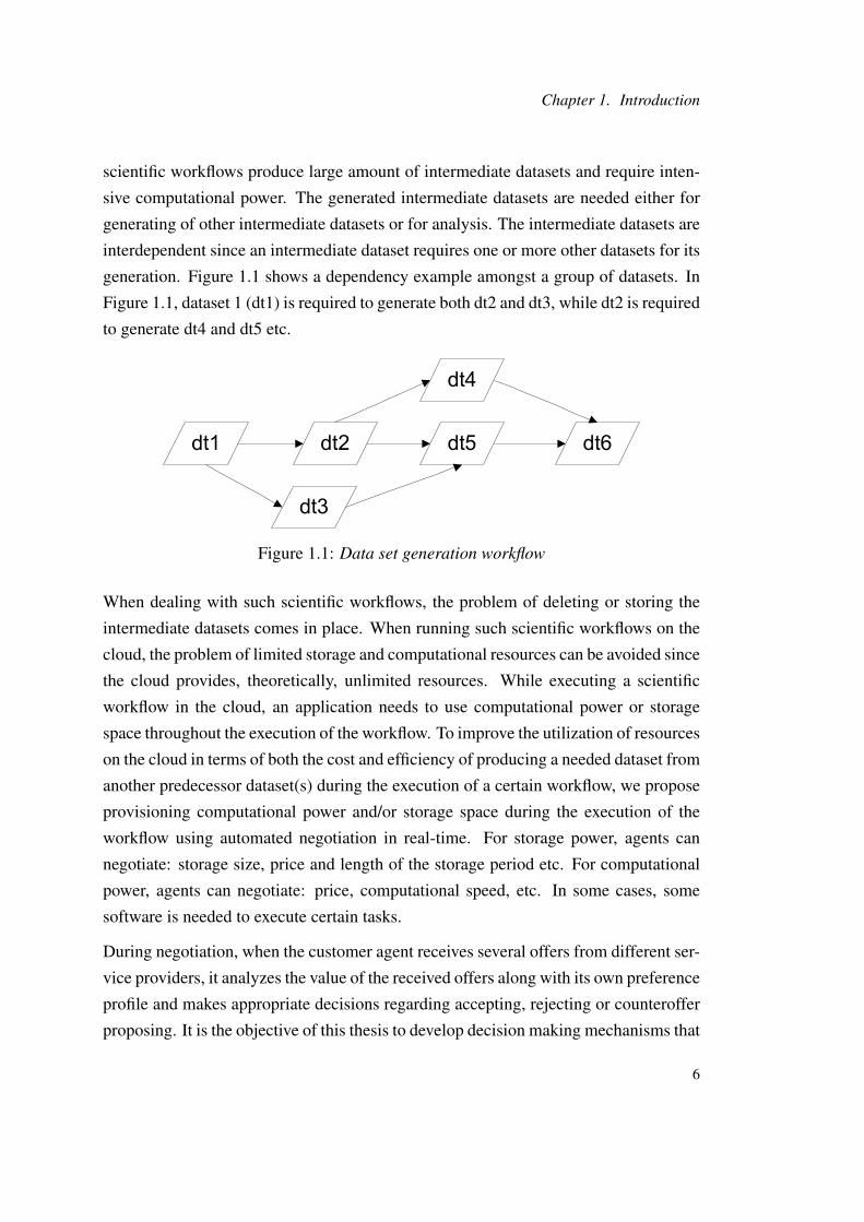
generation. Figure 1.1 shows a dependency example amongst a group of datasets. In
Figure 1.1, dataset 1 (dt1) is required to generate both dt2 and dt3, while dt2 is required
to generate dt4 and dt5 etc.
Figure 1.1: Data set generation workflow
When dealing with such scientific workflows, the problem of deleting or storing the
intermediate datasets comes in place. When running such scientific workflows on the
cloud, the problem of limited storage and computational resources can be avoided since
the cloud provides, theoretically, unlimited resources. While executing a scientific
workflow in the cloud, an application needs to use computational power or storage
space throughout the execution of the workflow. To improve the utilization of resources
on the cloud in terms of both the cost and efficiency of producing a needed dataset from
another predecessor dataset(s) during the execution of a certain workflow, we propose
provisioning computational power and/or storage space during the execution of the
workflow using automated negotiation in real-time. For storage power, agents can
negotiate: storage size, price and length of the storage period etc. For computational
power, agents can negotiate: price, computational speed, etc. In some cases, some
software is needed to execute certain tasks.
During negotiation, when the customer agent receives several offers from different ser-
vice providers, it analyzes the value of the received offers along with its own preference
profile and makes appropriate decisions regarding accepting, rejecting or counteroffer
proposing. It is the objective of this thesis to develop decision making mechanisms that
6
1.2. Usage Scenarios
enable the consumer agent to take effective negotiation decisions in real-time during
negotiation. Using automated negotiation in the cloud has the following advantages:
1. A scientific workflow may not know in advance the future computational and
storage resources needed. Instead of buying resources before starting the work-
flow, an agent can negotiate with the providers of cloud resources to provision
resources in real time. In this case the workflow will use the minimum needed
resources during its execution.
2. Since there are multiple resource providers in the cloud, automated negotiation
in real-time takes the advantage of existing multiple providers in increasing the
bargaining power of the buyer negotiator.
3. During negotiation, the workflow controller can decide whether to store a certain
dataset or delete a dataset depending on the received offers from the resource
providers.
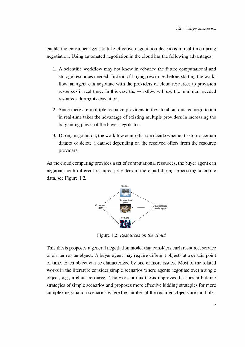
As the cloud computing provides a set of computational resources, the buyer agent can
negotiate with different resource providers in the cloud during processing scientific
data, see Figure 1.2.
Figure 1.2: Resources on the cloud
This thesis proposes a general negotiation model that considers each resource, service
or an item as an object. A buyer agent may require different objects at a certain point
of time. Each object can be characterized by one or more issues. Most of the related
works in the literature consider simple scenarios where agents negotiate over a single
object, e.g., a cloud resource. The work in this thesis improves the current bidding
strategies of simple scenarios and proposes more effective bidding strategies for more
complex negotiation scenarios where the number of the required objects are multiple.
7

Chapter 1. Introduction
1.2.2 Holiday Booking Scenario
This scenario is well known in the service oriented domain (e.g., [96][7][98]) where
a customer seeks a holiday package including a flight, a hotel and a car, see Figure
1.3. The automated one-to-many negotiation is a flexible approach for provisioning a
holiday package. It is known that travelers prefer certain dates and travel times, have
certain preferences over hotel bookings, such as hotel location (e.g., within a city or
outside the city) and hotel rating, e.g., 5 star hotel. For choosing a car, the traveler
may have certain preferences over the model and make of the car, its color etc. The
price can be one of the important issues but not the only one. Figure 1.3 shows that
each service has multiple attributes (issues) to be negotiated over between a traveler
and service providers.
Figure 1.3: Travel booking scenario
The auction models for service provisioning are not flexible since they focus on one
negotiation issue (usually price) and provide a limited number of predefined packages.
As Figure 1.3 shows, each service can have multiple negotiation issues. In addition,
each service can have multiple providers. The one-to-many negotiation allows a cus-
tomer agent to interact with different service providers concurrently. A negotiating
agent who receives multiple offers from service providers can analyze the received
offers and determine its next decision, either to accept one of the received offers or
to offer a new proposal. The coordination problem in that context is to find the best
match between the issue values of the different services taking into consideration the
preference profile of the customer agent and the value of the received proposals.
Most of the related works do not consider negotiation over multiple objects (e.g., ser-
vices) concurrently. This thesis proposes effective negotiation strategies for a buyer
agent negotiating concurrently with multiple seller agents over multiple objects.
8

1.2. Usage Scenarios
1.2.3 Supply Chain Scenario
A supply chain consists of all the intermediate points between the raw materials and
customers through which raw materials are acquired, processed, and delivered [44].
For example, the intermediate points can be: suppliers, warehouses, factories, etc.
Using a mediator agent to help in the negotiation process between two agents repre-
senting two firms is proposed in [41] where the negotiating agents aim to coordinate
their production sequences. Duan et al. propose a negotiation framework to tackle the
supplier-manufacturer problem where agents negotiate on the delivery schedules. The
issues of negotiation can include time, quantity and price [28]. The authors consider
that the delivery schedules for the supplier-manufacturer form an integral part of an
agent’s local optimization problem.
Supply chain management is a critical task for business success. As supply chain
management is concerned with the moving of material in a consistent manner, material
procurement is an essential part of the supply chain management. Figure 1.4 shows that
a factory, which can be represented by a buyer agent, interacts with three sources of
raw materials that can be represented by three raw material seller agents. The raw
material can contain negotiation issues such as price, quantity, delivery date etc.
Figure 1.4: Supply chain
Adopting the one-to-many negotiation model for solving the material procurement
problem in the supply chain can empower customers where there are multiple suppliers
in the market. In this case, when the customer negotiates with multiple suppliers, the
customer can benefit from the different proposals received from the suppliers by either
accepting the best proposal or offering new proposals. This thesis aims to empower
the customer agent by providing it with the appropriate decision making mechanisms
in such scenarios.
9
Chapter 1. Introduction
Just-in-time (JIT) manufacturing is a managerial philosophy that depends on procur-
ing the only needed materials or parts for running manufacturing processes. The JIT
manufacturing reduces both, the amount of inventory and the amount of waste [147].
When the JIT model is used by a manufacturing system, automated negotiation can
add a value to the JIS. When a certain amount of material or some parts are needed by
a manufacturing system, the system conducts concurrent negotiations with a number
of suppliers to negotiate critical issues such as quantity, price and delivery time of the
required parts or material. Introducing the automated negotiation in the JIF automates
the process of procuring materials which improves the efficiency and the effectiveness
of delivering the right materials at the right time.
As the case with the previous two sections, most of the related works in the literature
consider the problem of a single object of a single issue negotiation. In case of the
supply change management, most negotiations involve multiple issue negotiation or
multiple object negotiation. This thesis improves the current negotiation mechanisms
of simple scenarios and presents novel algorithms to handle complex negotiation sce-
narios.
1.3 Research Questions
Since the objective of this thesis is to investigate the coordination problem in the one-
to-many negotiation in multi-agent systems under the assumptions that agents do not
disclose their private information and the only available information for an agent dur-
ing negotiation is the offers received from its current opponents, this thesis addresses
the following main research question:
Can the bidding strategy for multiple concurrent one-to-many negotiations becoordinated by adapting an agent’s negotiation strategy parameters during nego-tiation?
The main question can be subdivided into the following research question:
1- Convexity of the Concession Curves: the convexity degree of a curve determines
10

1.3. Research Questions
its slop at a certain point. Changing some parameter of the curve equation can change
its slop. In the time-dependent offer generation tactics [33], changing the β value
results in changing the convexity of the concession curve. The first subquestion can be
formulated as follows.
• Can the approach of adapting the convexity of concession curves during multi-
ple concurrent negotiations be an effective method in improving one or more of
the negotiation performance criteria?
2- Negotiation Meta-Strategy: a meta-strategy is a strategy that uses more than one
type of negotiation tactic. For example, the concession and trade-off are two different
negotiation tactics that can be used during negotiation according to some rules. The
second subquestion can be formulated as follows.
• Can the approach of alternating between different negotiation tactics during
multiple concurrent negotiations be an effective approach in improving one or
more of the negotiation performance criteria?
3- Local Reservation Values: the local reservation values refer to the reservation val-
ues of the common issues of different negotiation objects. We assume that the global
reservation value of common issues is fixed throughout negotiation while it is possi-
ble to update the local reservation values of the common issues of certain negotiation
objects as a response to some changes in the negotiation environment. The third sub-
question can be formulated as follows.
• Can the approach of adapting the local reservation values during multiple con-
current negotiations be an effective method in improving one or more of the
negotiation performance criteria?
4- Multi-Level Coordination: When an agent negotiates over multiple objects given
that each object has multiple providers, then the agent needs to analyze the behaviors
of all opponents over all objects (global coordination level) and analyze the behaviors
of opponents over each particular object which is the local coordination level. For each
coordination level, the agent controls one or more negotiation strategy parameters in
the coordination process. The fourth subquestion can be formulated as follows.
11
Chapter 1. Introduction
• Can the approach of managing negotiation strategies at both, the global leveland local level during multiple concurrent negotiations be an effective method
in improving one or more of the negotiation performance criteria?
The answers to the research questions are discussed in chapter 8.
1.4 Contributions
The dynamic coordination in concurrent one-to-many negotiation involves managing
the negotiation strategy dynamically during negotiation for multiple instances (inter-
actions) of concurrent negotiations. The main body of this work investigates the dy-
namic bidding strategy in one-to-many negotiation. The bidding strategy determines
how an agent calculates the value(s) of its next offer(s). The proposed coordination ap-
proach considers the level of cooperation of the opponents in the terms of their offered
concessions in the current negotiation interaction. The previous data about the past
negotiations are not considered. The reason is that agents can be situated in dynamic
environments and their goals can be changed from one negotiation to another which
reduces the value of the historical data.
The main contributions of this thesis can be summarized as follows.
• Propose an extended negotiation model that emphasizes the notion of negoti-ation objects and allows for describing a variety of negotiation scenarios.
The proposed negotiation model is general and can be used to describe a wide
range of possible negotiation scenarios. It emphasizes the notion of a negotia-
tion object that allows for describing complex negotiation scenarios that involve
multiple objects, multiple negotiation issues and multiple providers for each ob-
ject.
• Analyze the possible negotiation scenarios in the one-to-many negotiation anddefine a set of scenarios that requires coordination, these scenarios are namedcoordination scenarios.
Considering the three main negotiation cornerstones, the negotiation objects, the
negotiation issues per object and the number of providers per object, most of the
12
1.4. Contributions
negotiation interaction types can be classified accordingly. A subset of the pos-
sible negotiation scenarios is identified and named coordination scenarios. The
identified coordination scenarios are the one-to-many negotiation types. This
work mainly investigates the coordination problem in the defined coordination
scenarios.
• Propose and evaluate new mechanisms that coordinate the bidding strategyfor a buyer agent dynamically during negotiation.
The main objectives of the mechanisms are to achieve effective and robust results
in terms of the utility rates and the agreement rates. In the case of multiple
issues, the proposed mechanisms aim at improving the Nash product rates as
well. Coordinating the bidding strategy comes as a response to the behaviors
of the opponents that exist in the current negotiation. The work involves the
investigation of five coordination scenarios.
For each scenario, one or more coordination mechanisms that manage the bid-
ding strategy (negotiation strategy) dynamically during negotiation are proposed
and validated. The solution to the coordination problem depends on the idea
of managing one or more negotiation strategy components during negotiation.
The convexity of a concession curve, the local reservation values and the types
of negotiation tactics are chosen for adaptation during negotiation. Most of the
works presented in this thesis focus on developing and validating the coordina-
tion mechanisms.
• Propose a new Iterative Offer Generation (IOG) bidding strategy that is com-petitive and cooperative at the same time.
The IOG mechanism involves two offer generation tactics: IOG-trade-off tactic
and IOG-concession tactic. Both tactics are used to generate counteroffers for
the proposed meta-strategy. The IOG-trade-off tactic proposes different coun-
teroffers that have the same utility in every negotiation round. Once the utility
level is changed, the new counteroffers are generated according to the new util-
ity. The IOG-concession tactic concedes in every negotiation round according
to a predefined amount. The difference between the proposed IOG-concession
tactic and other types of concession tactics is the that the IOG-concession tactic
considers that agents can have divergent preferences over issues. Therefore it
13

Chapter 1. Introduction
concedes more on the issues that are believed to be of high importance to the
opponent.
1.5 Thesis Outline
This thesis is structured into eight chapters as follows.
Chapter 2 is the background and related work part. It introduces the basic concepts
in automated negotiation and coordination and presents the related work. The chapter
first introduces briefly the multiagent systems paradigm, then it moves to introduce the
automated negotiation and approaches to automated negotiations including game the-
ory, learning and reasoning, and heuristic-based approaches. The argumentation-based
negotiation is also introduced briefly. Next, the dependencies and coordination is dis-
cussed including possible sources of dependencies in the negotiation context. Finally,
the related work in the one-to-many negotiation is presented.
Chapter 3 presents a novel negotiation model that captures various negotiation scenar-
ios. The model emphasizes that the negotiation object is one of the main components
that are necessary for describing any negotiation scenario. The model introduces the
term of delegate for describing an agents’ component that can negotiate with other
agents on the behalf of the agent. The utility functions that are used to evaluate offers
are also presented. Finally, since an object can have one or more negotiation issues,
an agent needs to decide when to accept an offer, the offers’ evaluation decisions are
discussed.
Chapter 4 is the coordinated negotiation and solution approach chapter. It presents
the coordination problem in the one-to-many negotiation and the solution approach.
In addition, it classifies the possible negotiation scenarios and defines a subset called
the coordination scenario set which is the study target of this thesis. In addition, the
difference between the global reservation value and the local reservation values is pre-
sented. Finally, the general experimental settings and the simulation environment is
introduced.
14
1.5. Thesis Outline
Chapter 5 presents coordination approaches for two coordination scenarios. The first
scenario is when a buyer agent is negotiating with multiple seller agents over one object
that contains a single negotiation issue. The coordination approach for this scenario
is based on managing the convexity of the concession curve during negotiation. The
second scenario is similar to the first one except that the number of negotiation objects
are more than one distinct object. One coordination approach considers the behaviors
of all seller agents across all objects (global approach) and a second one considers the
behaviors of the seller agents of each object alone, hence it is called the local approach.
The first approach is based on managing the local reservation values whereas the sec-
ond one is based on adapting the convexity of the concession curve. The combination
of both approaches is called a hybrid approach. In addition, the chapter presents an
empirical analysis for the different measures that can be used to analyze the behaviors
of the opponents. The results of the experimental work are presented and discussed.
Chapter 6 tackles the coordination scenario when a buyer agent seeks to procure a
single object characterized by multiple issues. The buyer agent negotiates with multi-
ple providers concurrently for the sake of reaching one agreement. A meta-negotiation
strategy is proposed to manage the multiple concurrent negotiations initiated by a buyer
agent. The coordination approach introduces a mechanism that selects a certain tac-
tic to use according to the current cooperation level of the opponents. In addition,
a novel offer generation mechanism is proposed, the iterative offer generation (IOG)
mechanism to generate counteroffers. It includes both a IOG-trade-off tactic and a
IOG-concession tactic. The mechanism assumes that agents have divergent prefer-
ences over issues. Both tactics are cooperative and competitive. They are competitive
because they aim to maximize the utility gain of the proposing agents and cooperate
since they consider the preferences of the opponents when proposing counteroffers.
The experimental results are presented and analyzed.
Chapter 7 investigates the coordination scenario where a buyer agent seeks to procure
multiple objects given that each object is characterized by multiple issues and has a
single provider. The scenario describes a monopolistic market where each service or
product has one provider. The proposed coordination approach considers manipulating
the local reservation values for the common issues. In addition, a global coordination
15
Chapter 1. Introduction
mechanism is proposed for the coordination scenario where each object has multiple
issues and the buyer agent is in a non-monopolistic market where each object has mul-
tiple providers. The empirical results for the coordination mechanisms are presented
and discussed.
Chapter 8 is the conclusions chapter. It concludes the thesis, answers the research
questions and discusses the thesis extensions and future work.
16
Chapter 2
Background and Related Work
After a brief introduction to the multiagent systems, the automated negotiation is in-
troduced and its application domains are highlighted. The approaches to negotiation
is presented next. This chapter starts with the game theory based approaches followed
by a discussion of the learning and reasoning methods used in negotiation. It also
presents different heuristic tactics used to generate offers and counteroffers during ne-
gotiation. Finally, the argumentation based negotiation approach is discussed briefly.
The next part of this chapter discusses dependencies and coordination by highlighting
possible interdependencies between the subjects of negotiation. The last part discusses
the relationship between coordination and negotiation. It presents short introduction
on some of the multiagent system coordination mechanisms and shows how negotiation
is considered as one of the possible coordination mechanisms. This part emphasizes
that the aim of this thesis is to coordinate concurrent multi-bilateral negotiations. In
addition, the relevant related work on the one-to-many negotiation focusing on the
different mechanisms proposed in the literature to coordinate multiple concurrent ne-
gotiations is presented.
2.1 Multiagent Systems Paradigm
The widespread connectivity amongst electronic devices provided by the Internet opens
the door for building large scale distributed applications and systems that span over a
large number of connected machines. The cloud computing and the grid computing are
Chapter 2. Background and Related Work
amongst the most important outcomes of such complex network systems. Electronic
commerce is another innovative domain for doing business. In addition, the advances
in computer systems lead to new computing paradigms such as ubiquitous computing
[112].
Distributed systems are characterized by the fact that different entities are connected
and are able to exchange messages and information. A multiagent system is a dis-
tributed computing system consisting of interacting software agents that can be used
to model and solve different real world problems such as business process management
[60], fault diagnosis in power systems [94], traffic management [17], etc. Task alloca-
tion [15] [83] and resource allocation [20] are two important problems in multiagent
systems that captured the attention of many researchers. The main differences between
the multiagent systems and the classical distributed systems is that the multiagent sys-
tems consist of intelligent and autonomous entities called agents where the agents are
self-interested entities that act to achieve its predefined goals [131] [57]. In addition,
agents in multiagent systems can have different owners in terms of their design and
implementation and may have even conflicting goals [159].
Multiagent systems model is suitable for: 1) uncertain, complex and dynamic environ-
ments 2) where agents are natural metaphors and used to model many environments as
societies of cooperating or competing agents such as most organizations 3) distribution
of data, control or expertise where centralized approaches are difficult to implement 4)
to solve the problem of dealing with legacy systems by wrapping a legacy component
with an agent layer [159]. An agent can represent a human, a robot or a software sys-
tem. In this manuscript, a software agent refers to a software system since software
agents are assumed to engage in negotiation where some agents represent buyers and
other agents represent sellers.
Some complex problems, especially those characterized by some social behavior, can
be modeled as multiagent systems since multiagent systems are enhanced distributed
systems equipped with components that are able to reason and make autonomous deci-
sions. Examples of such complex systems are socio-economic systems and biological
systems. In the electronic commerce domain, an electronic market can be modeled as
a virtual place where buyer agents, seller agents and broker agents meet and trade. In
general, agents in the electronic commerce are modeled as self-interested agents. In
this thesis, the following definition of a self-interested agent is assumed.
18
2.1. Multiagent Systems Paradigm
Definition 2.1. (Self-interested agents)
A self-interested agent is an agent who aims to maximize its gain from any interaction
with any other agent or with the environment without having the intension to harm
other agents or the environment. When there is room for a win-win outcome of an
interaction, the agent is willing to cooperate.
The above definition implies that a self-interested agent is a rational agent. The fol-
lowing is the formal definition of a rational agent.
Definition 2.2. (Rational agents)
A strict rational agent selects an option opi over an option opj if the expected utility
(EU) of opi is greater than the expected utility of opj , formally, a strict rational agent
selects opi iff EU(opi) > EU(opj). On the other hand, a weak rational agent selects
opi over opj iff EU(opi) ≥ EU(opj).
The rationality of agents can entail a thorny problem; there are situations where an
agent does not have enough computational resources or time for enumerating all the
possible options or decisions, which means that agents are rationally bounded. In such
situations, an agent aims to find a good or satisficing rather than an optimal solution.
The bounded rationality was first discussed in [140] in the context of a human decision
maker. To overcome this problem, heuristic decision making methods were proposed
[141]. Heuristic methods will be discussed later.
The above definitions are consistent with the characteristics of a self-interested agent
considered in the game theoretic models. From the definition above, the self-interested
agent is not necessary a bad agent since it does not have the intension to harm other
agents and it is willing to cooperate in case of existing a win-win situation. In addition,
type of agents we consider in this thesis are not benevolent agents.
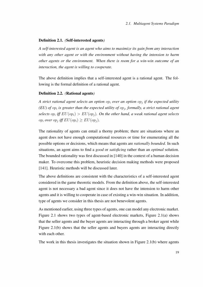
As mentioned earlier, using three types of agents, one can model any electronic market.
Figure 2.1 shows two types of agent-based electronic markets, Figure 2.1(a) shows
that the seller agents and the buyer agents are interacting through a broker agent while
Figure 2.1(b) shows that the seller agents and buyers agents are interacting directly
with each other.
The work in this thesis investigates the situation shown in Figure 2.1(b) where agents
19

Chapter 2. Background and Related Work
Figure 2.1: Agent-based electronic market structures
interact amongst each other without a broker agent. The reason is that, in reality, there
would be trust problems if a broker agent or a mediator agent is introduced. In addi-
tion, an extra overhead in terms of the communication cost will be experienced in case
of adopting a mediator-market model. However, Figure 2.1(b) includes three forms
of interactions: one-to-one, one-to-many and many-to-many, see Section 2.2. As men-
tioned previously, this thesis addresses the coordination problem of an agent interacting
concurrently with multiple other agents through negotiation in terms of managing the
bidding strategy for the agent on the one-side dynamically during negotiation.
2.2 Automated Negotiation
Negotiation is proven to be an effective conflict resolution method and has been used
extensively throughout history to settle conflicts between nations, groups and individ-
uals [117]. Negotiation is a challenging research field in many disciplines including
economics [124][145], political sciences [42], law [156], psychology and sociology
[27][113], anthropology [50] and applied mathematics [51].
Scholars from the Harvard Negotiation Project have proposed a method called princi-
20
2.2. Automated Negotiation
pled negotiation or negotiation on the merits [43]. The principled negotiation focuses
on four points that define a negotiation method that can be used in many situations.
The points are: people, interests, options and criteria. The first point emphasizes the
separation of people from the problem. In many cases negotiators deviate from the
main problem into personal disputes which will not help in solving the original ne-
gotiation problem. The interests point means that the focus of negotiation should be
on the interest, not positions. For example, if two people are arguing against open-
ing or closing a window, we need not to think about closing or opening the window,
we rather need to think about the interests of each individual from having the window
opened or closed to find a reconciled solution. The options point focuses on generat-
ing a variety of possibilities before deciding on what to do. It means that negotiators
should explore many options that may include adding more negotiation issues to the
negotiation problem and not leaving money on the table, i.e., reach a Pareto-optimal
solution. A solution is Pareto-optimal if and only if no agent can increase its utility
without affecting negatively the utility of other agent. The criteria point means that
the result of negotiation should be based on some objective standard. The agreement
needs to be based on fairness that meets certain standards, if known, such as market
value or scientific merits. For more details about the principled negotiation, see [43].
The reason behind introducing the principled negotiation here is that automated negoti-
ation using agents meet most of the principled negotiation points. For example, agents
have no personal view of the problem and the separation of people from the problem
is achieved. Agents are able to negotiate over interests not positions. In multi-issue
negotiation, agents can have many options that make them indifferent. In addition,
the principle of a win-win outcome is related to the third point, i.e., the options point.
Many negotiation techniques aim to achieve a win-win agreement. Moreover, many
automated techniques are designed to achieve a fair outcome (e.g., [31] [79]) which is
related to the criteria point.
The interest in the automated negotiation accompanied the recent advances in com-
puter network systems and communication technologies that facilitate the interaction
between software systems. For more than a decade, automated negotiation received
tremendous attention from researchers (e.g., [71] [164][30][33][68][37][40]). The
work on automating the negotiation process results from the fact that computer sys-
tems are becoming more intelligent, more connected and the delegation in decision
21
Chapter 2. Background and Related Work
making are increasingly being granted to computer systems. Consequently, computer
systems are becoming more autonomous and they need to interact to cooperate and
coordinate their actions to achieve their goals. Negotiation is one of the most effective
methods for managing the inter-agent dependencies at run time [58]. Automating the
negotiation process can help negotiate complex contracts [68]. According to Sand-
holm, the automation of negotiation [127]:
can save labor time of human negotiators, but in addition, other sav-
ings are possible because computational agents can be more effective at
finding beneficial short-term contracts than humans are in strategically
and combinatorially complex settings.
Improving the results of negotiation in terms of utility rate and/or agreement rate is
another advantage. In addition, negotiation may improve the social welfare of the
agency [36].
Automated negotiation borrows from other disciplines such as Game Theory, Eco-
nomics, Artificial Intelligence and Psychology. However, the related literature suggests
that three areas related to automated negotiation are of most importance [61] [80]:
• Negotiation Protocols: rules of encounter. This covers the participants (e.g.,
buyers and sellers) in the negotiation process, the permissible messages (e.g.,
sending a bid) amongst the participants, the negotiation states (e.g., negotiation
is active) and the events that cause the change in a negotiation state, e.g., bid
accepted.
• Negotiation Objects: a negotiation object can be characterized by a single is-
sue such price or more, e.g., price, quality, delivery time etc which is called the
object structure. An agreement entails agreement over the issues of an object.
The negotiation protocol determines the type of operation that can be done on
an agreement including the structure and the content of the agreement. There
are three possible operations that can be done to the agreement structure (set
of negotiation issues) and its content during negotiation: 1) both are fixed and
the opponents(s) can take (accept) or leave (reject) the offer 2) opponents can
propose counteroffers with different issue values from the received ones 3) op-
22
2.2. Automated Negotiation
ponents can change the structure of the agreement by adding or removing issues
during negotiation which is sometimes called issue-manipulation [33].
• Decision Making Models: the set of algorithms or methods an agent uses to
determine its next offer or counteroffer, i.e., the bidding strategy. The deci-
sion making models can be game theoretic based models, heuristic based mod-
els or argumentation-based approaches. The decision making models must be
aligned with the negotiation protocol and is affected by the operation allowed on
the agreement structure and its contents. In addition to the adopted negotiation
protocol, the set of issues and their types (i.e., an issue can take continuous of
discrete values) affect the range of a possible decision and the intricacy of the
decision making models [33].
In some auction models (e.g., English auction, Vickrey), the protocol allows buyer
agents only to bid on an issue and the room for employing different decision models
is limited since the dominant strategy for a buyer agent is to bid up to its reservation
value. The reservation is defined as the minimum/maximum acceptable value of an
issue. It is minimum when an agent (e.g., a seller agent) is in a position to gain a
resource such as money and maximum when an agent (e.g., a buyer agent) is in a
position to lose a resource such as money too.
In cases where a protocol does not describe an optimal strategy for an agent (e.g., the
alternating offer protocol), the decision making models and mechanisms receive the
main attention. This is the case where agents can bargain to reach an agreement. As-
suming fixed values for the agreement structure does not allow for bidding, bargaining
or strategic conduct. In summary, the settings of any of the above factors can affect the
possible set of negotiation outcomes.
Given the assumption that agents can bargain by exchanging offers and counteroffers,
negotiation can be classified into two types [67]:
1. Distributive negotiation: This type of negotiation assumes that a gain for one
agent is a loss for another. It is described as zero-sum game in the game theory
terminology. This type is also called positional bargaining. Distributive nego-
tiation exists if the negotiating agents have the same preference profile on the
negotiation object structure. For example, if the negotiation object contains the
23
Chapter 2. Background and Related Work
price issue then a gain for one agent during negotiation means a loss for one or
more other opponents.
2. Integrative negotiation: This type of negotiation exists when agents negotiate
over multiple negotiation issues given that agents have divergent preferences
over some or all issues. In case of integrative negotiation, agents have a chance
to reach a win-win agreement. This kind of win-win agreement can happen
because an agent may concede on an issue that is less important to him and more
important to its opponent(s) and vice versa.
The type of negotiation affects the decision making mechanism used by agents during
negotiation. Both of the above types are considered in this thesis. When the negoti-
ation is distributive (mainly when agents are negotiating over an object containing a
single issue), the decision making mechanisms are purely competitive while the de-
cision mechanisms can be competitive and cooperative at the same time in case of
integrative negotiation.
Automated negotiation has the potential of leading to a giant step forward in many ap-
plication domains. The main application candidate domains are: electronic commerce
(e.g., [101][103]), supply chain management (e.g., [120][157]), task scheduling and
allocation (e.g., [166][65]) and resource allocation for grid and cloud systems (e.g.,
[138][2]). Another potential application domain where automated negotiation can play
an important role is the dynamic load management of the power grid that allows for
both, cost-effective use of electricity production capabilities and customer satisfac-
tion [9]. Brazier et al. propose a component-based multi-agent system that manages
electricity load using negotiation [9]. Three application scenarios are presented and
discussed in Section 1.2.
In the service oriented domain, agents usually negotiate to establish the service level
agreements (SALs) over the quality of service (QoS) under negotiation (e.g., [134][162]).
QoS is the non-functional characteristic of a service (e.g., reliability) which distin-
guishes between functionally equivalent services. It is the focus of competition be-
tween providers of functionally similar services. A competitive criterion in the service
oriented domain is the flexibility in the number of possible QoS options that is avail-
able for customers to choose from. The current offer-based methods of QoS show
either little or no flexibility in the possible number of available options for the combi-
24

2.2. Automated Negotiation
nations of the QoS configurations. The service configuration flexibility problem stems
from the fact that in many cases, the number of possible combinations of different at-
tribute values of services is large. When a service is characterized by several issues,
then automated negotiation can be a flexible solution for establishing the SLA between
a customer and a provider.
The reason is that the provider does not need to enumerate varying service character-
istics by recounting the possible number of values that can be assigned to different
attributes of each negotiation object. In theory, when the issues are of a continuous
type, the number of possible SALs is infinite. Negotiation can be considered as a search
mechanism where agents jointly search the SLAs space for a possible agreement over
a certain SLA.
Web services composition is an important application domain where automated negoti-
ation can play an important role in the process of procuring different services. Besides
that an agent can search for a certain service provider(s), an agent can negotiate on
the behalf of its owner over the nonfunctional characteristics of a web service such
as response time, throughput, reliability, etc. Using agent technologies to conduct the
process of provisioning web services can be more efficient than using manual methods
that consume time, effort and cost more. For example, a coordinated-negotiation ar-
chitecture is proposed [21] for web-service composition to ensure end-to-end QoS. In
addition, the results of manual procuring of web services can be less efficient in terms
of procuring the most suitable web services in terms of quality of service.
In multiagent systems, there are three forms of interactions determined by the number
of interacting partners and their respective positions. The basic form is the bilateral
interaction where two opponent agents interact. For example, B1 and S4 agents in
Figure 2.1(b) conduct bilateral interaction. The second form is the one-to-many in-
teraction where an agent interacts with multiple agents. In Figure 2.1(b), agent B2
interacts with agents S2 and S3. The last form is the many-to-many interaction where
multiple agents interact with multiple other agents. Different market mechanisms can
be represented by one of these interaction forms. For example, the English auction can
be modeled as the one-to-many form where many buyers interact with one seller. The
reverse English auction can also be represented by the one-to-many form where many
sellers interact with one buyer. The double continuous auction can be represented
by the many-to-many form. The interaction between agents can be either a one-way
25

Chapter 2. Background and Related Work
model or a two-way model. The one-way interaction model refers to auctions while
the two-way interaction model refers to negotiation where agents exchange offers and
counteroffers.
One of the first explicit architectures for the one-to-many negotiation was presented
in [115] where the buyer agent consists of sub-negotiators and a coordinator. The
sub-negotiators negotiate concurrently with a set of seller agents given that each sub-
negotiator negotiates with one seller. As mentioned earlier, this thesis investigates
mainly the situation of a buyer agent negotiating concurrently with seller agents for
the purpose of reaching one or more agreements over one or more negotiation objects.
During the last decade, work has been done to address the one-to-many negotiation as
an alternative mechanism to the single-sided auction [106] [48] [105] [161] [3] [2].
Adopting the one-to-many negotiation as an alternative to the single-sided auction has
many advantages. Not only does the agent on the one side receive offers, but it also
proposes counteroffers to each individual agent on the many side. Accordingly, the
chance of reaching an agreement will improve since each agent in the negotiation pro-
cess analyzes the previous offers in the current negotiation encounter which aims at
predicting the preference structure of its opponents and proposes counteroffers that
might improve the chance of reaching an agreement.
To shed more light on the advantages of adopting concurrent negotiation over the
single-sided auction, the following few points provide more information [105]:
• when agents seek agreement over multiple attributes or issues, a buyer can select
an offer from a set of offers proposed by the seller agents in case of a reverse
auction and a seller can select an offer from a set of offers offered by the buyers
in a forward auction. In both cases, the buyer in the first case and the seller in
the second case do not have the chance to ask for modification of any of the
proposed offers. In the multi-bilateral concurrent negotiation, an agent has the
chance to respond and ask for a specific value for each issue. This is important
since buyers and sellers can have divergent preferences over different issues. For
example, a buyer is willing to offer a premium price for having an item delivered
within 24 hours while other buyers can wait one week for the same item to
be delivered for paying a lower price. In other words, the chance of reaching
an agreement will improve since the agent on the ‘one’ side in the negotiation
26
2.3. Approaches to Negotiation
process may analyze the previously received offers in the current negotiation
encounter which aims at predicting the preferences of its opponents and tries to
propose counteroffers that might improve the chance of reaching an agreement.
It is obvious that the multi-bilateral concurrent negotiation improves the search
for agreement(s) process since the approach allows buyers and sellers to search
for offers that meet their criteria more efficiently.
• when a buyer agent receives multiple offers from different sellers, its bargaining
power will improve and its negotiation strategy can be different against each
seller. For example, some sellers might be desperate for reaching a deal and that
fact can be used by the buyer to secure a good deal.
• the agreement reached in a certain negotiation encounter can affect (help) other
negotiations. For example, a buyer can not accept a worse deal than an existing
one.
• the time for reaching an agreement can be reduced in comparison with time
needed by auctions since some auctions need to wait for a certain time before
announcing any agreement. In the concurrent negotiation approach, a buyer can
accept an offer at anytime and finish negotiation before the deadline.
The downside of using the multi-bilateral concurrent negotiation approach instead of
auction models is the communication cost and the need for coordination mechanisms
to manage the negotiation strategies of agents.
2.3 Approaches to Negotiation
The negotiation objective criteria vary. In competitive environments, each agent aims
to maximize its gain regardless of the gain of other agents. In other situations, agents
seek to maximize both, the individual gain the system gain. As the bidding strategy is a
critical part in the negotiation process since it is the process by which an agent decides
on the value and the content of the offer/counteroffer for the next negotiation round,
the focus in most negotiation literature is on devising bidding strategy techniques that
can achieve an optimal solution to the negotiation problem. Given the fact that au-
tomation of the bidding process is complex, it is difficult to find an optimal strategy for
27
Chapter 2. Background and Related Work
a dynamic process such as negotiation [82], various negotiation approaches are pro-
posed in the literature to automate the negotiation process, e.g., [33]. There are three
main negotiation approaches: game theory-based, argumentation-based and AI-based
approaches. The following sections discuss each briefly.
2.3.1 Game Theory-Based Approaches
In many cases, the negotiation problem is treated as a bargaining problem which is
defined by Rubinstein as [125]:
Two individuals have before them several possible contractual agree-
ments. Both have interests in reaching agreement but their interest are not
entirely identical. What “will be” the agreed contract, assuming that both
parties behave rationally?
Game theory is a mathematical tool that can be used to answer that bargaining question
under certain assumptions. Game-theory is a branch of economics that is used to study
and analyze how self-interested agents make decisions during their interactions [109].
In their book titled ‘The Theory of Games and Economic Behaviour’ [154], John von
Neumann and Oskar Morgenstern invented the mathematical theory of games in 1944.
The proposed mathematical framework was limited since it is applicable only under
some strict conditions. Since then, the framework has gone under many iterations of
refinements to make it work under less strict conditions [123]. In the context of game-
theory, an agent can be defined as an entity with preferences that aims to maximize its
utility which is measured by a utility function [123]. The utility function of an agent
assigns a value (usually numeric) to the outcomes of the game.
Optimal strategy and equilibrium are two important keywords in game theory since
researches aim to find the optimum strategies for interacting agents that lead to equi-
librium considering their preference and possible alternatives. The most famous type
of equilibrium is Nash equilibrium. Two strategies st1 and st2 are said to be in Nash
equilibrium if an agent is playing st1 and its opponent agent can do no better than play
st2 and vice versa.
28

2.3. Approaches to Negotiation
Figure 2.2: Taxonomy of game theory
Negotiation is a bargaining problem where two or more agents have conflict of inter-
est over an issue or more and there is a possibility for achieving a mutually beneficial
agreement(s) and the agreement(s) needs approval from all parties. Bargaining theory
is a part of game theory that investigates and analyzes bargaining games. Game theory
can be divided into cooperative and non-cooperative game theory. A possible taxon-
omy of game theory is shown in Figure 2.2 [77]. The cooperative game theory aims
at finding a solution while given a set of possible outcomes rather than on the specific
rules of the game or the negotiation process. The chosen solution usually needs to
satisfy some conditions such as being fair or stable. These conditions or properties are
called axioms. For example, if the condition is that the two bargainers gain the same
utility upon an agreement, then this would be an axion [77] [47].
The eminent work of Nash results in defining a unique solution satisfies four properties
which are called Nash axioms [102]. Assuming that players are rational, the axioms
are: 1) The outcome is invariance to equivalent payoff representation. This means that
the outcome of the bargaining process is not affected by a utility function transforma-
tion and keeps the same ordering over preferences 2) Pareto optimality. There is no
other agreement that can make both players better off or make one player better off
without making the other player worse off. 3) Independence of irrelevant alternatives.
This means that the outcome is not related to irrelevant outcomes, i.e., if the current
agreement is feasible, other alternative agreements are not considered 4) Symmetry. If
the players are indistinguishable, they should gain the same utility, i.e., no discrimina-
tion in selecting the agreement.
29

Chapter 2. Background and Related Work
When the previous assumptions hold, Nash proves that there is a unique solution
(Nash-bargaining solution) that maximizes ((u1(x1) − d1).(u2(x2) − d2)) which is
called Nash-product. The u1(x1), u2(x2) are the pay-offs of the solutions x1 and x2respectively. In addition, d1, d2 are the payoffs in case of conflict outcome.
Kalai and Smorodinski argue against Nash’s third axiom and suggest a new axiomatic
solution called kalai-Smorodinski bargaining solution by replacing the third axiom of
Nash by the monotonicity property, see [63]. Since the outcome of the negotiation
process that is considered in this thesis depends on the interactions amongst agents,
the approach of cooperate game theory is not applicable here.
On the other hand, if a game has a well defined set of rules defined by a certain proto-
col that is known by the players before the start of the game, then the non-cooperative
game theory is the branch that handles such situations. The actions of each player at
each step during the game are determined by a bargaining strategy given the histori-
cal information of negotiation. The objective of the non-cooperative game theory is
to find the equilibrium strategy to define the rational behaviors of players, then the
rational behaviors of all players decide the outcome of the game. As mentioned be-
fore, Nash equilibrium is an example of such an equilibrium. For example, a strategy
equilibrium for a buyer agent and a seller agent who have unlimited negotiation time
is that each agent offers the minimum allowed concession in each negotiation round
until their offers match. There is no benefit for any player to deviate from this strategy
by conceding, for example, more than the minimum allowed concession. As Figure
2.2 shows, the non-cooperative game theory is divided into complete information and
incomplete information. In the complete information case, agents know about the pref-
erences of each other. Different protocols lead to different outcomes at the subgame
perfect equilibria (SPE) [77]. Games such as ultimatum [99], alternating offers [125]
and monotonic concessions [122] were analyzed and investigated to find the SPE.
The mechanism design and sequential bargaining are two approaches usually used to
study the non-cooperative game theory with incomplete information. The mechanism
design abstracts the process of bargaining and uses the players’ private information to
find the bargaining solution [77].
In sequential bargaining games, the outcome is reached by exchanging offers and coun-
teroffers between the players. The sequential bargaining games are divided into one-
sided incomplete information and two-sided incomplete information, see Figure 2.2.
30
2.3. Approaches to Negotiation
Assume that a buyer and a seller would like to reach an agreement over a certain issue
using the alternating offer protocol (i.e., by exchanging offers and counteroffers) and
if one player (say the buyer) knows about the reservation price value of the seller, then
the game is called a one-sided incomplete information game. If both, the seller and the
buyer do not know anything about each other (e.g., reservation values) then the game is
called a two-sided incomplete information. When analyzing the two-sided incomplete
information games, researchers assume that each player has a limited number (e.g., 2)
of types to simplify the analysis, see [16].
Finally, using game theory, it is possible mathematically to analyze games in terms of
finding the equilibrium fulfilling strategies. However, to do that, game theory applies
strict conditions. It assumes that agents have the ability to assign ‘utility values’ for all
possible outcomes. In many cases, a utility function that maps an outcome to a numeric
value does not exist. For humans, it is difficult even to rank different outcomes espe-
cially when negotiating over objects characterized by multiple issues. Another limi-
tation is that game theory generates specialized models that are applicable in certain
types of interdependent decision-making and fails in producing a general model. In
addition, game theory assumes that players or agents are rationally unbounded which
means that they know all possible solutions within a feasible range of outcomes or can
find them within an acceptable computational time. Finally, players are assumed to
have full knowledge about the environment and about the opponents in terms of their
preferences over different outcomes. The assumption about total rationality and full
knowledge are unrealistic since agents are computationally bounded and rarely know
the outcome preferences of their opponents. Game theory is suitable in terms of analy-
sis and can be used in automated negotiation when the relevant conditions are assumed
to exist, see [77] [47] [58].
To enable adopting automated negotiation in more realistic situations, the artificial
intelligence (AI) techniques are used in automated negotiation to relax the strict as-
sumptions of game theory. The AI techniques use learning and reasoning methods that
can help agents in learning and reasoning about their opponents’ models and adapt
their behavior to the current situation. The next section discusses briefly some of the
AI techniques that are relevant to automated negotiation.
31
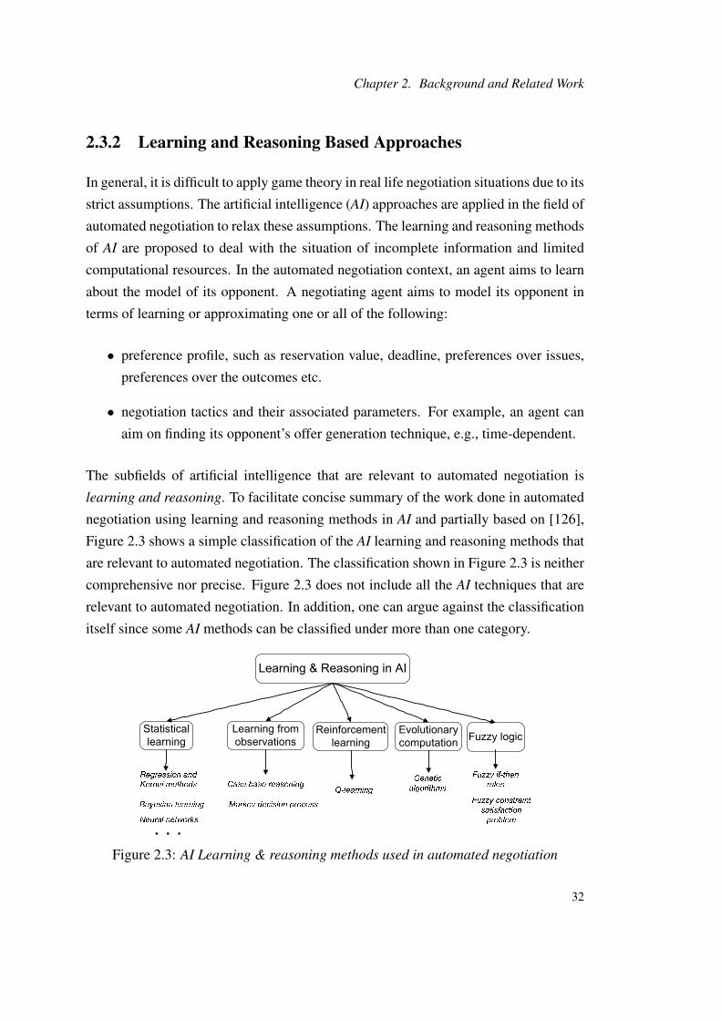
Chapter 2. Background and Related Work
2.3.2 Learning and Reasoning Based Approaches
In general, it is difficult to apply game theory in real life negotiation situations due to its
strict assumptions. The artificial intelligence (AI) approaches are applied in the field of
automated negotiation to relax these assumptions. The learning and reasoning methods
of AI are proposed to deal with the situation of incomplete information and limited
computational resources. In the automated negotiation context, an agent aims to learn
about the model of its opponent. A negotiating agent aims to model its opponent in
terms of learning or approximating one or all of the following:
• preference profile, such as reservation value, deadline, preferences over issues,
preferences over the outcomes etc.
• negotiation tactics and their associated parameters. For example, an agent can
aim on finding its opponent’s offer generation technique, e.g., time-dependent.
The subfields of artificial intelligence that are relevant to automated negotiation is
learning and reasoning. To facilitate concise summary of the work done in automated
negotiation using learning and reasoning methods in AI and partially based on [126],
Figure 2.3 shows a simple classification of the AI learning and reasoning methods that
are relevant to automated negotiation. The classification shown in Figure 2.3 is neither
comprehensive nor precise. Figure 2.3 does not include all the AI techniques that are
relevant to automated negotiation. In addition, one can argue against the classification
itself since some AI methods can be classified under more than one category.
Figure 2.3: AI Learning & reasoning methods used in automated negotiation
32

2.3. Approaches to Negotiation
If an agent can model its opponent, it can use relevant decisions to maximize its utility
gain or achieve other negotiation objective criteria. The most used learning meth-
ods are classified under statistical learning where agents apply statistical techniques
to predict and/or to learn information about their opponents. Learning can be offline,
online or both. The offline learning uses previous information (e.g., outcomes of pre-
vious negotiation encounters) in the learning process while the online learning uses the
information available during the current negotiation encounter. In most cases, the dy-
namic information that are available to the agents in the current negotiation encounter
are the current negotiation threads, see Section 3.2. Domain knowledge is another
source of information. In addition, a probability distribution over unknown parameters
(e.g., deadline) is a useful source of information for agents. Finally, some approaches
assume a predefined set of models about the opponent.
Regression methods are used in negotiation to estimate the parameter(s) of a given
negotiation decision function using the thread of the current negotiation encounter.
Regression methods are also used to predict the type of negotiation tactic (e.g., time-
dependent) used by the opponent assuming that the opponent uses a predefined set of
tactics [11] [12]. In one-to-many negotiation, [135] uses linear regression to predict
the future proposals of an opponent. The prediction result is used to decide whether an
agent should continue negotiating or accept the best offer in an acceptable list and quit
negotiation. The coordination process involves deciding on proceeding or terminating
the concurrent negotiation. The work in [135] assumes that agents are negotiating over
a single issue.
A limitation of the regression methods is the assumption about the decision models
of the opponent. In addition, the online prediction using regression methods can be
computationally expensive.
On the other hand, Coehoorn and Jennings use the kernel density estimation KDE
method to approximate the preferences of an opponent over various issues in multi-
issue negotiation [22]. The KDE is a non-parametric statistical method that can be
used to estimate the probability density function of a stochastic variable. The authors
use the difference between the last two offers of the opponent to find a relation between
this difference and the preference in terms of weight the opponent has for each issue.
Once an agent approximates the weight that its opponent places on each issue, it uses
the trade-off method to generate its offer aiming to reach a win-win agreement. The
33
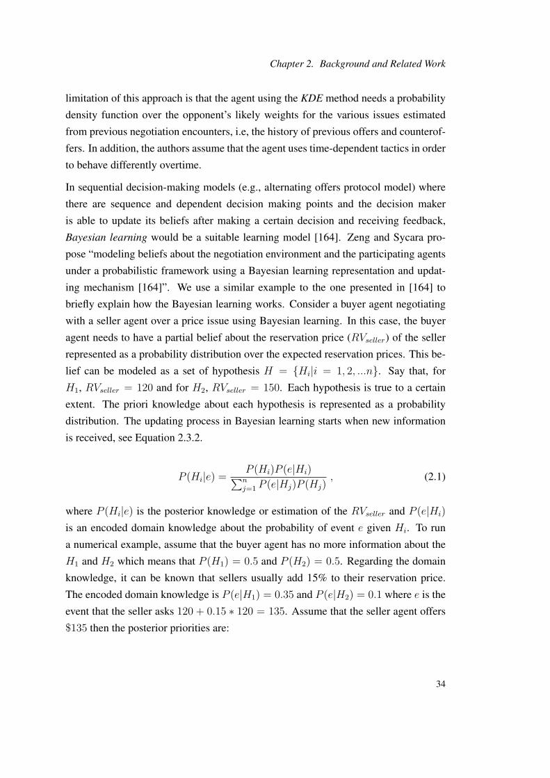
Chapter 2. Background and Related Work
limitation of this approach is that the agent using the KDE method needs a probability
density function over the opponent’s likely weights for the various issues estimated
from previous negotiation encounters, i.e, the history of previous offers and counterof-
fers. In addition, the authors assume that the agent uses time-dependent tactics in order
to behave differently overtime.
In sequential decision-making models (e.g., alternating offers protocol model) where
there are sequence and dependent decision making points and the decision maker
is able to update its beliefs after making a certain decision and receiving feedback,
Bayesian learning would be a suitable learning model [164]. Zeng and Sycara pro-
pose “modeling beliefs about the negotiation environment and the participating agents
under a probabilistic framework using a Bayesian learning representation and updat-
ing mechanism [164]”. We use a similar example to the one presented in [164] to
briefly explain how the Bayesian learning works. Consider a buyer agent negotiating
with a seller agent over a price issue using Bayesian learning. In this case, the buyer
agent needs to have a partial belief about the reservation price (RVseller) of the seller
represented as a probability distribution over the expected reservation prices. This be-
lief can be modeled as a set of hypothesis H = Hi|i = 1, 2, ...n. Say that, for
H1, RVseller = 120 and for H2, RVseller = 150. Each hypothesis is true to a certain
extent. The priori knowledge about each hypothesis is represented as a probability
distribution. The updating process in Bayesian learning starts when new information
is received, see Equation 2.3.2.
P (Hi|e) =P (Hi)P (e|Hi)∑nj=1 P (e|Hj)P (Hj)
, (2.1)
where P (Hi|e) is the posterior knowledge or estimation of the RVseller and P (e|Hi)
is an encoded domain knowledge about the probability of event e given Hi. To run
a numerical example, assume that the buyer agent has no more information about the
H1 and H2 which means that P (H1) = 0.5 and P (H2) = 0.5. Regarding the domain
knowledge, it can be known that sellers usually add 15% to their reservation price.
The encoded domain knowledge is P (e|H1) = 0.35 and P (e|H2) = 0.1 where e is the
event that the seller asks 120 + 0.15 ∗ 120 = 135. Assume that the seller agent offers
$135 then the posterior priorities are:
34
2.3. Approaches to Negotiation
P (H1|e) =0.5 ∗ 0.35
0.35 ∗ 0.5 + 0.1 ∗ 0.5= 77.78%
P (H2|e) =0.5 ∗ 0.1
0.35 ∗ 0.5 + 0.1 ∗ 0.5= 22.22%
The buyer agent updates its knowledge about the reservation value of the seller accord-
ingly. For more information, see [163][164].
Bayesian learning is used to learn both the issue preferences and the issue priorities of
an opponent in multi-issue negotiation [53]. One of the proposed model assumptions
is that an agent has some knowledge about issue priorities of the opponent. Another
assumption is that a hypothesis space of predefined function types about the opponent
is assumed.
The Bayesian learning assumes some knowledge to work such as the encoded specific
domain knowledge which is not always available. In addition, the Bayesian framework
does not provide a negotiation strategy in the form of concession behavior. Applying
the Bayesian learning in one-to-many negotiation is more difficult since an agent needs
to have some information about a large number of agents which is difficult to do in
reality given that agents negotiate in an open and dynamic system.
Neural networks do not assume any relationship between the input and out variables
since this kind of relationship will be learned by the neural network itself. A neural
network needs a training on a training dataset when using offline learning, or it can
start processing information after a certain number of offers are exchanged between
agents. For example, [13] uses both, offline and online neural network training to
model the negotiation process in a time-series style. The neural network used in [108]
was trained offline and then online before testing it. The trained neural network is used
by a seller agent negotiating with a buyer agent over the price issue. Using the neural
network, the seller agent needs to predict the next price proposal of the buyer agent
given that the buyer agent has already sent three proposals. The experimental results
show that the seller agent using neural network achieves more deals when compared
with a seller agent using Q-learning when the deadlines are long.
The drawback of using neural networks is that they need training before they can per-
form well. In addition, if an agent using a neural network is negotiating with an oppo-
35
Chapter 2. Background and Related Work
nent agent playing different strategies from the ones that were used in the training set,
the neural network could have unpredictable behavior.
The idea of Case-based reasoning (CBR) is to solve a new problem using or adapting
previously found solution(s) used to solve similar problems. The CBR mechanism elic-
its information and learns from previous cases histories, hence it does not need explicit
information about some domain knowledge [155]. In negotiation, an agent adopting
CBR, uses previously stored cases for comparison and decision making during nego-
tiation encounters. The cases that are kept in the case database and used later are the
ones who achieved successful outcomes in negotiation. Sycara was one of the first to
use CBR in the PERSUADER program, that resolves labor disputes using negotiation
where “contracts, impasses and arguments are used as basis for Case-Based Reasoning
at performing” the required tasks [148]. Argumentation and CBR are used in [167] to
manage the negotiation strategy in e-commerce. Matos and Sierra use CBR as a tech-
nique to assign parameter values to negotiation tactics and determine the weights that
will be used to combine those tactics [93] whereas the fuzzy rules are used to adapt the
chosen solution considering the environmental information before making new offers.
A possibilistic case-based reasoning is used in [10] to predict negotiation outcomes
for a potential set of negotiation partners. The partner with the highest score or rate
is selected to be a negotiation partner. However, this approach was not used in the
process of managing the negotiation strategy during negotiation.
One of the drawbacks of using CBR in negotiation is that an agent requires a large
number of previously stored cases in order to achieve good results since agents in
many cases, exist in open and dynamic environments. In addition, a CBR agent may
not be able to reason during negotiation when it faces a situation where its opponent
behaves differently from any stored case.
The Markov decision process (MDP) is a stochastic process that has been used to
model the negotiation process, e.g., [101][149]. Narayanan and Jennings model a bi-
lateral negotiation as two non-stationary MDPs because each agent views the state
space differently, and they are non-stationary processes due to the environmental dy-
namics which makes the probability of transition from one state to another vary over
the negotiation time [101]. In their model, the authors assume that agents have some
information about the transition function represented as probabilistic knowledge. In
addition, they assume the Markov property in the system (i.e., the state transition of a
36
2.3. Approaches to Negotiation
system depends only on the current state) as they argue that only the current state of
the system triggers the process of selecting an effective strategy. However, they state
that more work needs to be done to verify that claim.
The state space in [149] is modeled as a set of negotiation tactics. An agent using
the MDP method needs to negotiate with several other agents to build an empirical
probability distribution of the tactics after which the agent updates the empirical prob-
abilities by learning from other agents’ responses. A decision making strategy based
on a tractable Markov chain model of negotiation process is proposed [3] to help an
agent adopting that model to make a decision on whether to accept the best received
proposal from a set of partners or to keep on negotiating in case the expected utility
in the next proposals will be better. The main drawback of using the MDPs is that it
requires a meaningful probability distribution over the state transition matrix in order
to deliver effective outcomes.
Reinforcement Learning (RL) is a learning method where agents learn by experience.
An Agent observes the state of its environment and takes action. Depending on the
action it takes, it receives either a positive or negative reward. When an agent has
the opportunity to take a new action, it selects the action that brings him a positive
reward. This process of learning is repetitive and the agent is expected to learn over
many repetitions [146].
In negotiation, agents adapt their negotiation strategies according to the feedback re-
ceived after using a particular strategy. The feedback can be an opponent’s response to
using a certain strategy. For example, after using a certain strategy, the opponent may
accept, reject or quit negotiation.
Q-learning is the most used type of reinforcement learning. An agent using Q-learning
updates the Q-value when it selects an action a given a state s, see Equation 2.2. In
negotiation, the Q-value is updated at every negotiation round for the chosen action a
taken while in state s.
Q(s, a)← Q(s, a) + α[R(s′) + γmaxa′
Q(s′, a′)−Q(s, a)] , (2.2)
where maxa′ Q(s′, a′) is maximum expected reward (e.g., utility) of the next state s′.
The learning rate α controls the amount of Q-value update, α ∈ [0, 1]. If a Q-learning
agent assumes α = 0 then the agent does not learn (i.e., it does not update the Q-
37
Chapter 2. Background and Related Work
value) since it keeps the oldQ-value. When α = 1, the agent considers the most recent
information. The factor γ ∈ [0, 1] is the discount factor. If γ = 0 then the agent
considers the current rewards. If γ = 1 then the agent will look for a high reward in
the future. R(s′) is the immediate reward after choosing the state s′.
In automated negotiation, Q-learning is used to select a negotiation strategy from a set
of different combinations of negotiation tactics (e.g., [14]) where an agent learns to
select an appropriate negotiation strategy during negotiation. The choice of a certain
strategy can be either rewarded or punished. The Q-learning agent is expected to per-
form well after a certain number of iterations depending on the number of states, e.g.,
strategies.
The problem of using Q-learning in negotiation is that Q-learning has proven to have
slow convergence towards near-optimal solutions in comparison with other techniques
such as genetic algorithm based classifier systems [108]. Another problem is that, an
agent using Q-learning has to reason whether to exploit the current situation or explore
other possible solutions.
Evolutionary computation methods are based on models of natural selection. The three
most popular forms of evolutionary computation are genetic algorithms, evolution
strategies and evolutionary programming. The genetic algorithms model evolution
at the level of genes. Evolution strategies model evolution at the level of individuals
competing for resources while evolutionary computation models evolution at the level
of species competing for resources [5].
A genetic algorithm starts with a randomly generated population. The population is
evaluated using a fitness function and with a probability related to the fitness of each
individual, an individual can be transferred into the next generation either unchanged,
mutated or created by the crossover method where information from two parents are
used to make a new individual. The process is repeated until some stop condition
becomes true. In negotiation, the evolutionary computation methods allow agents to
empirically learn using good negotiation strategies. A genetic algorithm based learning
technique is proposed in [107] for learning negotiation strategies. The strategies are
structured as sequential rules consisting of offers separated by thresholds. Each thresh-
old represents the utility of an offer. However, the model offers little expressiveness to
model strategies with even simple decision rules. Tu [150] proposes an approach based
on genetic algorithms that evolves from negotiation strategies where each strategy is
38

2.3. Approaches to Negotiation
presented as a finite state machine. Each strategy competes against other strategies and
is adapted over time depending on the completion outcomes using a genetic algorithm.
If the population size is not large, genetic algorithms can produce acceptable outcomes.
However, in real world scenarios, their application is limited due to the large number
of negotiation strategies. Accordingly, the population search space becomes large and
intractable.
Fuzzy logic is used in negotiation as a decision making approach for selecting an appro-
priate negotiation strategy considering current negotiation environmental conditions,
e.g., [93] [139]. When using fuzzy logic, it is important to choose a fuzzy model that
suits a certain system since fuzzy modeling is the most important issue in fuzzy logic
[144]. In automated negotiation, two main fuzzy logic models are used to model the
decision making process: the fuzzy if-then rules and the fuzzy constraint satisfaction
problem. The fuzzy rules are a set of rules applied to certain variables. When a certain
fuzzy rule is satisfied, a corresponding action is initiated. For a multi-input and single-
output system, the fuzzy rule looks like [144]: Ri : ifx1 is Ai1 and x2 is A
i2 ... and xn
is Ain, then y is Bi, where Ri is the ith rule, xj is the input variable and Aij and Bi
are fuzzy variables. Matos and Sierra use fuzzy rules to adapt the current mental state
of an agent by adapting the parameters of the negotiation tactics and their contribution
weighs in the next offer while considering the current environmental situation. Fuzzy
rules are used in [139] to manage the amount of concession during negotiation. They
take into consideration the negotiation environmental conditions such as competition,
deadlines, trading options, etc.
The problem of using fuzzy rules is that some knowledge and experience is needed to
set up the rules. In addition, it is difficult to change the rules during negotiation which
can be a problem in dynamic and open systems.
On the other hand, negotiation can be modeled as a constraint satisfaction problem [70]
since an agent has constraints and preferences that need to be satisfied during the nego-
tiation. To provide a more flexible model, negotiation is modeled as a fuzzy constraint
satisfaction problem (FCSP), e.g., [69][81] where the constraints are considered fuzzy
and presented by membership functions. In general, an agent using FCST to model
negotiation aims to reach an agreement that maximizes its gain, and when possible,
to maximize the opponent’s gain too, i.e., the agent aims to achieve a Pareto optimal
solution. The Prioritized FCSP approach is used in [81] to handle situations in which
39
Chapter 2. Background and Related Work
an agent is not able to describe precisely its preferences over negotiation issues, when
the agent’s constraints are fuzzy. For example, if an agent is searching for a nearby
inexpensive restaurant, then there is no precise acceptable preference over choosing a
restaurant. A certain restaurant could be partially satisfied or partially violated. For
more reasons on adopting the PFCSP, see [81]. The concept of priority in FCSP was
introduced to handle the matter of existing issues with different importance. Exiting
issues with different importance are the base of using trade-off in negotiation. For
more detail on using trade-off in negotiation, see Section 2.3.3.5. Finally, the model
assumes that agents exchange more information than the ones related to the values of
issues, such as constraints about the product the buyer agent intends to buy which lim-
its the applicability of the approach where only values over issues can be exchanged.
To wrap-up this section, the following are general comments about using learning and
reasoning AI techniques in automated negotiation:
• even though AI techniques relax the strict conditions assumed for applying game
theoretic techniques, i.e., complete knowledge and unbounded rationality, AI
techniques still require either partial knowledge represented as probability dis-
tribution over variables (e.g., Bayesian learning) or training before the start of
negotiation, e.g., neural networks
• most AI techniques are proposed for bilateral negotiation
• most AI techniques are designed for the situation where agents negotiate over one
object, and in most cases that object contains the price as the only negotiation
issue.
2.3.3 Heuristic-Based Tactics
Negotiation is a dynamic and non-deterministic process. The assumption is that agents
work under incomplete knowledge since the preferences over the negotiation out-
comes, the utility structure and the deadlines are considered private information for
each agent. The heuristic-based models provide approximate solutions to the problem
of the bidding strategy. The heuristic approaches can be used in different application
domains and allow an agent to show different behaviors in terms of its concession strat-
egy that help it to adapt to the current situation. The heuristic-based approaches are
40
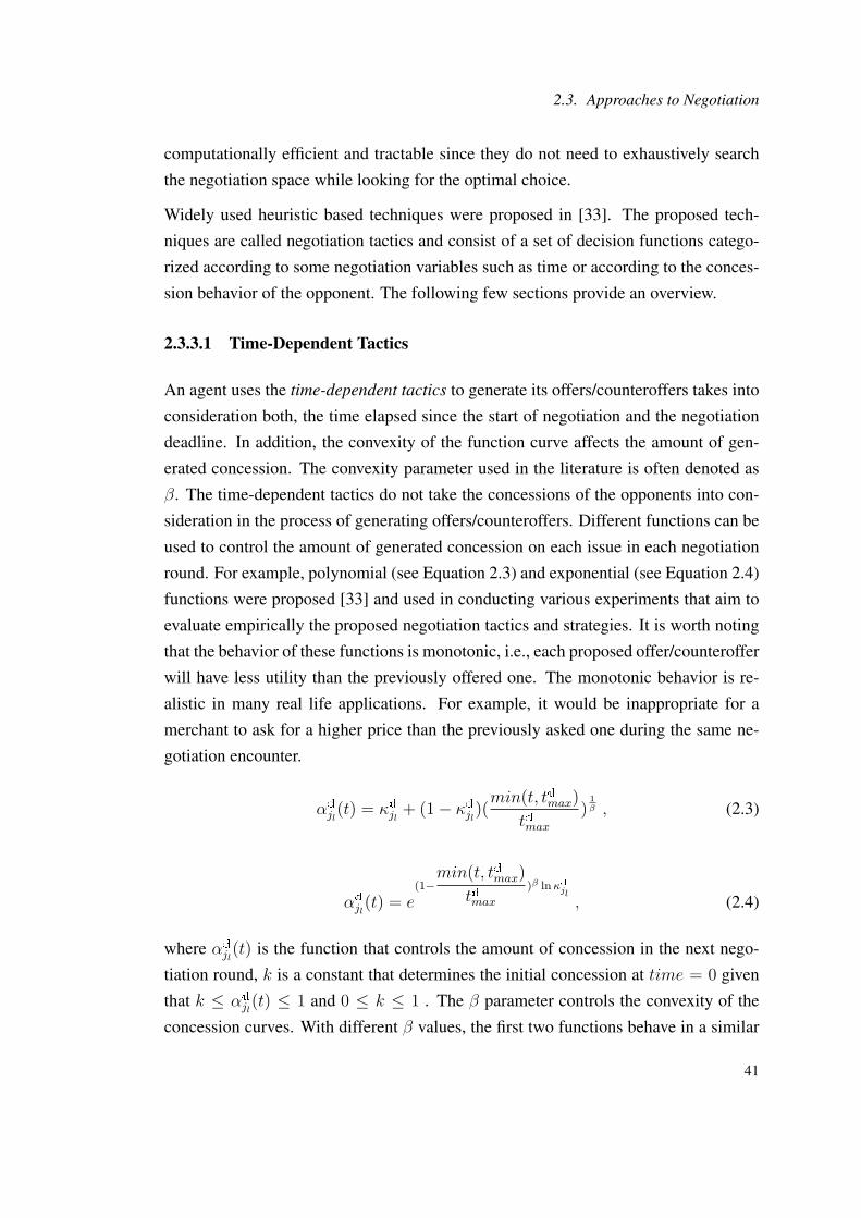
2.3. Approaches to Negotiation
computationally efficient and tractable since they do not need to exhaustively search
the negotiation space while looking for the optimal choice.
Widely used heuristic based techniques were proposed in [33]. The proposed tech-
niques are called negotiation tactics and consist of a set of decision functions catego-
rized according to some negotiation variables such as time or according to the conces-
sion behavior of the opponent. The following few sections provide an overview.
2.3.3.1 Time-Dependent Tactics
An agent uses the time-dependent tactics to generate its offers/counteroffers takes into
consideration both, the time elapsed since the start of negotiation and the negotiation
deadline. In addition, the convexity of the function curve affects the amount of gen-
erated concession. The convexity parameter used in the literature is often denoted as
β. The time-dependent tactics do not take the concessions of the opponents into con-
sideration in the process of generating offers/counteroffers. Different functions can be
used to control the amount of generated concession on each issue in each negotiation
round. For example, polynomial (see Equation 2.3) and exponential (see Equation 2.4)
functions were proposed [33] and used in conducting various experiments that aim to
evaluate empirically the proposed negotiation tactics and strategies. It is worth noting
that the behavior of these functions is monotonic, i.e., each proposed offer/counteroffer
will have less utility than the previously offered one. The monotonic behavior is re-
alistic in many real life applications. For example, it would be inappropriate for a
merchant to ask for a higher price than the previously asked one during the same ne-
gotiation encounter.
αdjl(t) = κdjl + (1− κdjl)(min(t, tdmax)
tdmax)
1β , (2.3)
αdjl(t) = e(1−
min(t, tdmax)
tdmax)β lnκdjl
, (2.4)
where αdjl(t) is the function that controls the amount of concession in the next nego-
tiation round, k is a constant that determines the initial concession at time = 0 given
that k ≤ αdjl(t) ≤ 1 and 0 ≤ k ≤ 1 . The β parameter controls the convexity of the
concession curves. With different β values, the first two functions behave in a similar
41
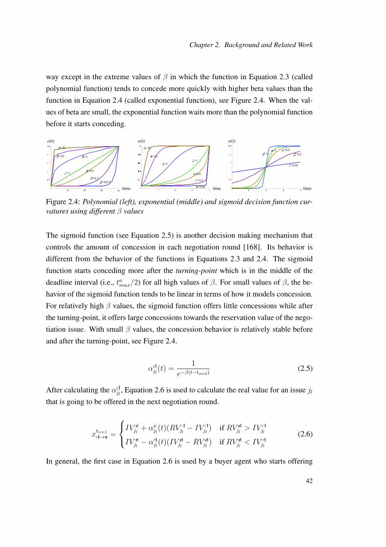
Chapter 2. Background and Related Work
way except in the extreme values of β in which the function in Equation 2.3 (called
polynomial function) tends to concede more quickly with higher beta values than the
function in Equation 2.4 (called exponential function), see Figure 2.4. When the val-
ues of beta are small, the exponential function waits more than the polynomial function
before it starts conceding.
Figure 2.4: Polynomial (left), exponential (middle) and sigmoid decision function cur-vatures using different β values
The sigmoid function (see Equation 2.5) is another decision making mechanism that
controls the amount of concession in each negotiation round [168]. Its behavior is
different from the behavior of the functions in Equations 2.3 and 2.4. The sigmoid
function starts conceding more after the turning-point which is in the middle of the
deadline interval (i.e., tamax/2) for all high values of β. For small values of β, the be-
havior of the sigmoid function tends to be linear in terms of how it models concession.
For relatively high β values, the sigmoid function offers little concessions while after
the turning-point, it offers large concessions towards the reservation value of the nego-
tiation issue. With small β values, the concession behavior is relatively stable before
and after the turning-point, see Figure 2.4.
αdjl(t) =1
e−β(t−tmid)(2.5)
After calculating the αdjl , Equation 2.6 is used to calculate the real value for an issue jlthat is going to be offered in the next negotiation round.
xtn+1
d→s=
IV d
jl+ αdjl(t)(RV
d
jl− IV d
jl) if RV d
jl> IV d
jl
IV d
jl− αdjl(t)(IV
d
jl−RV d
jl) if RV d
jl< IV d
jl
(2.6)
In general, the first case in Equation 2.6 is used by a buyer agent who starts offering
42
2.3. Approaches to Negotiation
the least amount of resources (e.g., money) to its opponent seller agent for buying
an object oi, while the seller agent starts asking for high amounts of resources (e.g.,
money) in exchange for the negotiation object oi.
The concession patterns shown by the functions in Equations 2.3 and 2.4 can be classi-
fied into three broad areas of behaviors that are controlled by the convexity parameter
β. The three behavior types are:
• Boulware, where β < 1. The Boulware agent makes small concessions in the
start of negotiation and continues until it reaches near its deadline where it offers
large amounts of concessions and reaches its reservation value when it meets
its deadline. This type of behavior represents an agent who is not desperate in
reaching an agreement quickly. This type of agent is rather aims to reach an
agreement with high utility.
• Linear, β = 1. The linear agent offers the same amount of concession in each
negotiation round and this linear behavior is applied strictly to the polynomial
decision function, see Equation 2.3. The behavior of the exponential function
(Equation 2.4 is nearly linear when β = 1. The linear behavior represents an
agent who balances between the time of agreement and the quality of that agree-
ment.
• Conceder, where β > 1. The conceder agent offers large concessions at the
beginning of negotiation then starts offering small concessions until it reaches
its reservation value at the deadline. The conceder type of agent represents a
situation where an agent is desperate in reaching an agreement regardless of the
quality of that agreement.
2.3.3.2 Resource-Dependent Tactics
As the name implies, the resource-dependent 2.3.3.1 tactics depend on the amount of
the available resources for determining the value of the offer/counteroffer in the next
negotiation round. In Equation 2.7, the resourcea(t) is a function that returns the
amount of available resources at time t, such as the number of the negotiating agents
or the number of the exchanged messages during negotiation etc. [33].
αdhj(t) = κdhj + (1− κdhj)e−resourced(t) (2.7)
43
Chapter 2. Background and Related Work
When the amount of the available resources are low, then the value of the function
αdhj(t) is high, which means that agent d needs to offer large concessions to improve
the chances of reaching an agreement. On the other hand, when the available resources
are high, agent d tends to offer small amounts of concessions. Time is a specific type
of resource and it will be the resource that is investigated in this thesis since time is a
critical factor for any negotiation process and the time-dependent tactics are a special
type of resource-dependent tactics.
2.3.3.3 Behavior-Dependent Tactics
Behavior-dependent tactics or Tit-For-Tat (TFT) family is another approach for gen-
erating offers. When an agent uses a behavior-dependent tactic to generate offers, it
imitates the behavior of its current opponent in terms of the opponent’s concessions.
The imitation procedure depends on weather the imitation takes into consideration the
recent or old amount of concessions offered by the opponent. In addition, the imitation
can be exact (where an agent concedes the exact amount of its opponent concession)
or proportional where an agent offers an amount of concession proportional to the
amount of concession offered by its opponent. To accommodate the stated imitation
factors, three behavior-dependent tactics (TFT) are proposed [33]. The type of TFT
shown Equation 2.8 is called Relative Tit-For-Tat where an agent finds the percentage
between two previously received offers then multiplies that percentage by its last offer.
For example, if δ = 1 and the last received offers by a seller agent are $18 and $16
at t = 1 and t = 3 respectively and the buyer agent offered $10 at t = 2 then the
buyer agent will propose (18/16) ∗ 10 = $11.25 at time t = 4. Equation 2.8 is ap-
plicable when n > 2δ. The δ in the TFT tactics determines whether an agent imitates
the recently received offers or the offers received some time back in the history of the
current encounter. If δ is small then the agent imitates the recently received offers. In
the following three equations, If IV d
jl< RV d
jlthen mindjl = IV d
jland maxdjl = RV d
jl,
otherwise mindjl = RV d
jland maxdjl = IV d
jl. Finally, the Max(., .) is a function that
returns the maximum value of its two arguments andMin(., .) is a function that returns
the minimum value of its two arguments.
xtn+1
d→s[jl] = Min(Max(
xtn−2δ
s→d[jl]
xtn−2δ+2
s→d[jl]
xtn−1
d→s[jl],min
d
jl),maxdjl) (2.8)
44

2.3. Approaches to Negotiation
The Random Absolute Tit-For-Tat tactic is shown in Equation 2.9. If an agent uses this
tactic, it imitates the concessions of its opponent exactly, i.e., in absolute terms. For
example, if a seller agent decreases its offer by $5 then the buyer agent increases its
offered price by $5 too. As said before, it is an exact imitation. A random function
(R(M) ∈ [0,M ]) is introduced in the tactic where M is the maximum amount by
which an agent would deviate from its imitation pattern. The random function R(M)
is introduced to break the cycle of exact imitation between agents.
xtn+1
d→s[jl] = Min(Max(x
tn−1
d→s[jl] + (x
tn−2δ
s→d[j]− xtn−2δ+2
s→d[jl]) + (−1)sR(M),mindjl),max
d
jl)
(2.9)
Again, the condition for Equation 2.9 applicability is that n > 2δ since an agent needs
to receive a minimum of 2 offers before applying the tactic. In Equation 2.9, if IV d
jl<
RV d
jlthen s = 0, otherwise s = 1.
The third TFT is the Averaged Tit-For-Tat (see Equation 2.10) where an agent finds the
percentage of an offer received ν steps back in the history of the current negotiation
encounter to the most recent received offer then multiply the resultant percentage by
the value of the last offered proposal by the agent. When ν = 1, it becomes similar to
the relative Tit-For-Tat tactic. If ν > 1, the agent is expected to offer more concessions.
xtn+1
d→s[jl] = Min(Max(
xtn−2ν
s→d[jl]
xtns→d
[jl]xtn−1
d→s[jl],min
d
jl),maxdjl) (2.10)
The above behavior-dependent tactics model different ways of imitation behaviors.
The success of each tactic can be tested empirically. For empirical results concerning
these tactics, see [33].
Another formulation is adapted [78] where an agent imitates the concession of its op-
ponent as shown in Equation 2.11. This will be referred to as Concession Tit-For-Tat.
Ctd
= A ∗ |xt−1d→s
[jl]− xt−3d→s[jl]|+ (1− A) ∗ |xt−2
s→d[jl]− xt−4s→d
[jl]| , (2.11)
whereCt is the amount of concession proposed at time twhich will be added to the last
offer of agent d if IV d
jl< RV d
jland deducted from the last offer when IV d
jl> RV d
jl.
A is the imitation factor, A ∈ [0, 1]. Formula 2.11 assumes the absolute value in the
45

Chapter 2. Background and Related Work
difference between the last two offers in order to accommodate for all types of issues,
i.e., whether their values are increasing or decreasing during negotiation.
To illustrate using Equation 2.11, assume that the turn is for agent d to propose an
offer where it sets A = 0.6. It means that the amount of concession (Ct) that will be
offered by agent d at time t consists of 60% of its previous concession and 40% of its
oppnent’s previous concession. If A = 0, then agent d imitates the exact concession
of its opponent and if A = 1 then it offers the same amount of concession it offered
previously. The concession Tit-For-Tat offers a flexibility to manage the amount of
imitation during negotiation by changing the amount of the concession factor A taking
into consideration some environmental changes such as behaviour of the opponents,
number of out side options etc. In addition, as the previous imitation methods provide
the flexibity in selecting recent or old concessions to imitate, the concession Tit-For-
Tat also provides the flexibility of sellectig either recent concessions or old concessions
to imitate.
In general, an agent takes into consideration the current negotiation thread in formu-
lating the behavior-dependent proposals and does not use old negotiation threads gen-
erated by previous negotiations.
2.3.3.4 Mixing of Tactics
When an agent uses a single negotiation tactic throughout the course of negotiation to
generate proposals, its strategy can be described as a pure-strategy or a non-strategic.
On the other hand, the strategic behavior can be either static or dynamic. The static
strategy in this context means that an agent first generates multiple offers by different
tactics. Each generated offer contributes to the final proposal according to the weight
that is previously assigned to each tactic. The weights that mix between tactics do not
change during negotiation. In dynamic strategy, the weights change during negotiation
in response to change in the opponent’s behavior [33]. However, for the experimental
work of this thesis, the static strategy indicates that an agent does not change any
negotiation parameter(s) during negotiation regardless of the number of tactics used
to generate an offer while the dynamic strategy indicates that an agent changes some
negotiation parameter(s) during negotiation even if that agent uses a single negotiation
tactic to generate a proposal.
To generate an offer, each tactic contributes some percentage (determined by a mixing
46

2.3. Approaches to Negotiation
weight matrix) to the value of the generated offer. For a dynamic strategy, the mixing
weights matrix are changed according to some factors that form the mental state of an
agent. IfMStd
is the mental state of an agent d at time t andMSd is the set of agent d’s
possible states. The MStd
combines both knowledge and attitudes. The knowledge is
about both the environment and the opponents. The attitudes include goals, designers,
intention etc. The change in the mental state of agent d can trigger a change in the
negotiation strategy including the change in the mixing weight matrix Γtn+1
d→s[35].
Γtn+1
d→s=
γj11 γj12 . . . γj1h
γj21 γj22 . . . γj2h...
......
...
γjp1 γjp2 . . . γjph
(2.12)
A row γjl in Equation 2.12 represents the percentages of contributions of different tac-
tics in the generated offer for the issue jl given that each γjl,i ∈ [0, 1] and∑h
i=1 γjl,i =
1. Agent d builds the Γtn+1
d→smatrix according to its mental state MSt
dat time t.
τtn+1
d→s=
τj11 τj12 . . . τj1h
τj21 τj22 . . . τj2h...
......
...
τjp1 τjp2 . . . τjph
(2.13)
The matrix τtn+1
d→sis the matrix of generated proposals using tactics 1, .., h for each
issue jl ∈ Jq at time (t + 1) by agent a where |Jq| = h. Equations 2.12 and 2.13
represent a multidimensional proposal for an object oi where oi is characterized by
the negotiation issues j1, ..., jp, i.e., oi ∼ Jq. The weighted proposal is defined as
follows [33].
Definition 2.3. (Weighted proposal) A weighted proposal xtn+1
d→s[jl] is a linear weighted
combination of proposals generated by a set of negotiation tactics 1, ..., h and de-
fined as: xtn+1
d→s[jl] =
∑hi=1 γjl,i ∗ τjli
For example, if the vector of negotiation tactic types of an agent d that is used in a cer-
tain negotiation instance (see Section 3.2) to generate proposals for the price issue is
<Boulware, linear, conceder, tft> and the associated weight row vector Γtn+1
a→b [price] =<
47

Chapter 2. Background and Related Work
0.35, 0.2, 0.15, 0.30 > and assume that τ tn+1
d→s[price] =< 40, 60, 80, 65 >, then the
xtn+1
d→s[price] = 0.35 ∗ 40 + 0.2 ∗ 60 + 0.15 ∗ 80 + 0.30 ∗ 65 = $57.5 and agent d sends
$57.5 as a counteroffer to agent s.
A multidimensional weighted proposal is a set of weighted proposals where xtn+1
d→s[Jq] =
xtn+1
d→s[j1], ..., x
tn+1
d→s[jh]. In other words, the multidimensional weighted proposal is a
proposal which consists of multiple values (one value per a negotiation issue) where
each value is a weighted proposal.
This method of mixing different tactics in generating a proposal has the advantage of
incorporating different factors that can play a role in determining the bidding strat-
egy of an agent such as the behavior of the opponents and state of resources, e.g.,
time. Other external environmental factors that many affect the urgency of reaching
an agreement can give more weight, for example, to the conceder tactic etc. When
the mental state (MS) of an agent changes, it changes the matrix Γtn+1
d→saccordingly.
Applying the weighted proposal method by an agent d decreases the probability of
predicting the negotiation strategy of agent d by its opponent especially when the ma-
trix Γtn+1
d→sis dynamic since there will be a regular pattern that can be analyzed by the
opponents of agent d.
As stated in Section 4.3, any change to any negotiation parameter is considered a
change to the negotiation strategy. The model proposed in this thesis assumes that
the Γtn+1
d→sis part of the negotiation parameters. Taking into account the mental state
of an agent, Γtn+1
d→s= f(MStn
d,Γtn
d→s) where f is a function that takes the mental state
and the mixing weight matrix of agent d at time t and returns Γtn+1
d→sthat is going to
generate weighted proposals at time (t+1). Realizing the function f will be discussed
in the following chapters.
2.3.3.5 Trade-off Generation Approach
Trade-off is a concept meaning that one can tolerate losing something for gaining
something else. This concept is widely used in real life especially in business. The
trade-off approach of generating offers is heavily investigated in the literature of auto-
mated negotiation (e.g., [34] [22] [19]). The Trade-off approach is important since it
is a method where negotiating partners can use to reach a win-win agreement instead
of reaching win-lose (zero-sum) agreement.
48
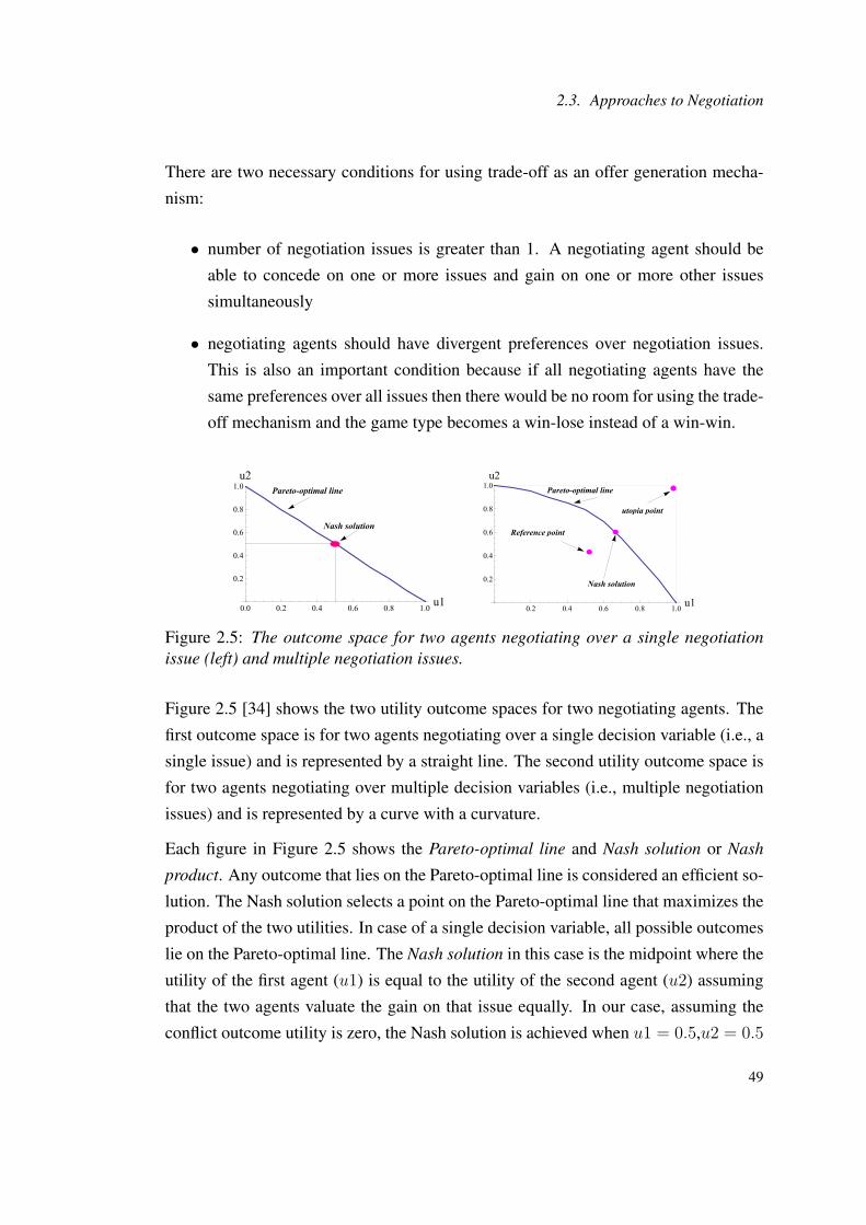
2.3. Approaches to Negotiation
There are two necessary conditions for using trade-off as an offer generation mecha-
nism:
• number of negotiation issues is greater than 1. A negotiating agent should be
able to concede on one or more issues and gain on one or more other issues
simultaneously
• negotiating agents should have divergent preferences over negotiation issues.
This is also an important condition because if all negotiating agents have the
same preferences over all issues then there would be no room for using the trade-
off mechanism and the game type becomes a win-lose instead of a win-win.
Pareto-optimal line
Nash solution
0.0 0.2 0.4 0.6 0.8 1.0 u1
0.2
0.4
0.6
0.8
1.0u2
Pareto-optimal line
Nash solution
Reference point
utopia point
0.2 0.4 0.6 0.8 1.0 u1
0.2
0.4
0.6
0.8
1.0u2
Figure 2.5: The outcome space for two agents negotiating over a single negotiationissue (left) and multiple negotiation issues.
Figure 2.5 [34] shows the two utility outcome spaces for two negotiating agents. The
first outcome space is for two agents negotiating over a single decision variable (i.e., a
single issue) and is represented by a straight line. The second utility outcome space is
for two agents negotiating over multiple decision variables (i.e., multiple negotiation
issues) and is represented by a curve with a curvature.
Each figure in Figure 2.5 shows the Pareto-optimal line and Nash solution or Nash
product. Any outcome that lies on the Pareto-optimal line is considered an efficient so-
lution. The Nash solution selects a point on the Pareto-optimal line that maximizes the
product of the two utilities. In case of a single decision variable, all possible outcomes
lie on the Pareto-optimal line. The Nash solution in this case is the midpoint where the
utility of the first agent (u1) is equal to the utility of the second agent (u2) assuming
that the two agents valuate the gain on that issue equally. In our case, assuming the
conflict outcome utility is zero, the Nash solution is achieved when u1 = 0.5,u2 = 0.5
49

Chapter 2. Background and Related Work
where u1 ∗ u2 = 0.25 which is the maximum possible combination between the two
utilities. It is like dividing the cake equally between two individuals. In case agents are
negotiating over multiple issues, the Nash solution is the point that is Pareto optimal
and lies on the line connecting the reference point to the utopia point. The reference
point can be computed as the utility outcome at the midpoint of each decision variable
[34].
In many real life scenarios, agents are negotiating under incomplete knowledge and it is
difficult to find optimal bargaining solutions such as Nash solution. Heuristic methods
are used to approximate the preference structure of the opponent as an approach to
reach near optimal solutions.
The trade-off generation approach in the context of automated negotiation is associated
with terms such as Pareto-optimality (see Section 2.2), social welfare and iso-curves
or indifference curves. The social welfare refers to the system utility. Social welfare
can be looked at either from the utilitarian or egalitarian point of views. The utili-
tarian principle is based on achieving the greatest total welfare. The total welfare of
a society is the sum of each individual utility in that society. The egalitarian princi-
ple is concerned about maximizing the utility of the most needy individuals in society
[97]. For example, Nash solution is considered more utilitarian than egalitarian [114].
kalai proposed a characterization of an egalitarian solution when the bargaining set
is convex, compact and comprehensive for a fixed number of individuals [62]. The
solution is characterized by being symmetric, having weak Pareto optimality and so
strong monotonicity is assumed. An egalitarian solution considers fair outcomes by
maximizing the more unfortunate individuals.
The indifference curve consists of the set of composite offers over a certain object that
have the same utility value. If the negotiation issues are of a continuous type, the
number of possible indifference curves are infinite.
Definition 2.4. (Composite offer) A composite offer is an offer that contains more
than one value. It happens when a negotiation object is characterized by more than
one issue in which case the offer proposed or received for this object is a composite
offer.
For example, a proposed composite offer may contain $10 for the price issue and 2 kg
for the weight issue of a certain material. Figure 2.6 shows three iso-curves, u1, u2 and
50

2.3. Approaches to Negotiation
u3. For example, all the points on the iso-curve u1 have the same utility level. In other
words, an agent is indifferent to any composite x and y values that lie on the curve u1.
The same applies to any iso-curve.
Figure 2.6: Iso-curves
For an agent who intends to keep the same aspiration level (i.e., utility value) while
negotiating with other agent(s), it can move along its current indifference curve trying
to propose offers with higher values to its opponent(s) given the fact the agents have
divergent preferences over issues. For example, consider a buyer agent and a seller
agent. Both are negotiating over an item containing the price and delivery_time issues.
The seller agent needs a long time to deliver the item and is willing to concede more
on the price. On the other hand, the buyer agent is more concerned about the price and
is willing to concede more on the delivery_time than the seller agent who may give
more concessions on the price and less concessions on the delivery_time which suits
the buyer agent’s preferences.
As a negotiation strategy, an agent should stay on its current indifference curve as
much as it can. The agent can stay on its current indifference curve without causing
the opponent agent to withdraw from negotiation by proposing trade-off offers that
may provide the opponent with more valuable offer(s) than the ones proposed pre-
viously. Given the fact that agents negotiate under incomplete knowledge, since the
utility structures, reservation values and deadlines are considered private information
for each, different methods are used to approximate the preference structure of the op-
ponent in the process of generating offers that may give higher values to the opponent
than the previously offered ones while staying on the current indifference curve.
Besides the mediated-negotiation (e.g., [31]) in which agents disclose some informa-
tion to a trusted third party that helps in reaching a Pareto-Optima agreement (or near
Pareto-optimal) agreements, the similarity (e.g., [34]) methods such as fuzzy similar-
51
Chapter 2. Background and Related Work
ity and shortest-distance (e.g., [73]) approaches are proposed to reach a near Pareto-
optimal outcome in multi-issue negotiation. In addition, the iterative-offer-generation
is a proposed method that enhances the chances of proposing offers that are of more
value to the opponent than the previously proposed ones [87]. The iterative-offer-
generation mechanism is discussed in Section 6.2.
The mediated-negotiation proposed in [31] searches for an optimal-agreement in bi-
lateral negotiation where the negotiation issues are of a continuous type. The media-
tor takes into consideration the preferred directions submitted by the two negotiating
agents. In each negotiation round, the mediator receives two proposals from the two
agents then it generates a new tentative agreement taking into consideration the jointly
improving direction. The negotiation process continues until the optimal solution is
found. However, due to the practical problems associated with using a mediator such
as trust, in many situations, it is difficult to use the mediated-negotiation approach.
The idea of using similarity between offers is investigated in [34]. The proposed al-
gorithm uses the fuzzy similarity principle to approximate the preference structure of
a negotiating opponent by modeling the domain of the decision variables. The hill-
climbing technique is used to search the apace of possible trade-offs for the offer that
is most likely to be acceptable by the opponent. It is easy to find similarity between
continuous issues such as a price, since if the difference between two prices is zero,
then the similarity is maximum. The problem in measuring similarity between the val-
ues of issues happens when the negotiation issues are of discrete types. For example,
a color can be an issue of negotiation. The color domain can be a set containing red,
blue, yellow, green, etc. The problem is that how can one measure the similarity be-
tween two colors such as red and blue? Faratin et al. propose creating a set of criteria
functions that can be used to associate each color in the color domain with a specific
number representing a certain criteria such as “warmness” of colors [34]. When an
agent decides on using the trade-off method, it generates a few counteroffers then it
selects the most similar one to the last received offer from the opponent given that the
agent generates the counteroffers at the same previous utility level, i.e., the agent stays
on its current indifference curve. However, the method needs some knowledge about
how the opponent places weights on the different issues. In addition, it is difficult to
find suitable techniques to measure similarity between discrete negotiation issues.
The shortest distance approach [74] finds the shortest distance between the last re-
52

2.3. Approaches to Negotiation
ceived offer and an offer on the current indifference curve. The empirical experimental
results presented in this paper show that agents achieve near Pareto optimal agree-
ments by using the shortest distance approach given that the negotiation issues are of
a continuous type. The preference of each agent is rational and strictly convex and
the monotonicity behavior is assumed. However, the negotiation model requires that
agents stay enough time in negotiation and propose a number of offers (to increases
the chances of finding a proposal that is close enough to the last opponent’s offer) in
each negotiation round. In addition, the approach assumes that both agents capture
their preferences using utility functions. However, in many real cases, agents can not
characterize their preferences by a utility function, because this function may not ex-
ist. Moreover, it is not clear when an agent should move from the current indifference
curve to another indifference curve. In addition, it is not clear how efficient the tech-
nique is in case the number of negotiation issues is large. Other trade-off approaches
are proposed, for example [119] assumes that negotiation issues have binary values in
estimating the opponent’s utility structure.
2.3.4 Argumentation-Based Negotiation
Argumentation-based negotiation (ABN ) is a relatively new approach where agents
exchange not only offers/counteroffers but also arguments. The arguments are pieces
of information that aim to change the mental state of an opponent. Changing the mental
state of an agent using an argument can be achieved by either justifying the proposed
offer or persuading (influencing) the opponent’s point of view or stance [59]. The in-
fluencing argument could be a promise for reward or a threat. For example, when a
project manager asks his/her employee to finish a task within a short period of time,
then the employee might disagree to that request as he/she needs more time. In this
case, the manger may promise a financial reward if the employee finishes the task
within a short period of time or threat to fire the employee if the task is not finished
within the requested time frame. An agent using the argumentation-based method may
ask to change the negotiation object or add more attribute(s) to the current negotiation
object. For example, if an employee asks his/her manager a pay raise then the man-
ager may reject the request. To overcome this problem, the number of working hours
attribute can be introduced to the negotiation as an argument where the employee asks
to keep the same rate of pay while reducing the working hours etc. [160].
53

Chapter 2. Background and Related Work
People usually use the argumentation concept during their daily negotiation interac-
tions. For example, a customer who would like to buy a laptop can visit different
shops to check prices and other related data. Then he/she can use the collected infor-
mation as an argument with a new shop manager saying that “I found a similar laptop
with a price of $330 and you are asking for $340”. This type of argument may con-
vince the shop owner to beat that price and sell that laptop for less than $330. If the
customer does not know about the prices of that type of laptop in other places, then
convincing the owner of the current store to sell that laptop for less than $330 would
be more difficult.
Since the classical negotiation approaches (i.e., game-theoretic and heuristic) of con-
flict resolution in multiagent systems focus on exchanging potential proposals accord-
ing to different protocols or on mechanism design that have limitation in achieving the
goal(s) of negotiation, argumentation-based negotiation can improve both the chance
of reaching an agreement and the quality (in terms of utility, fairness etc.) of the
agreement for agents engaged in negotiation. In general, agent using game-theoretic
or heuristic models are allowed only to exchange proposals; agents are unable to ex-
change additional information to persuade or influence other agents. In case agents
have limited information about the environment and/or about other agents especially
when the rational choices of some agents depend on the choices of other agents, the
traditional methods of negotiation-based conflict resolution limit the quality of the ne-
gotiation outcomes [160].
The ABN approach has the potential to improve the outcomes of the negotiation pro-
cess when compared to the game-theoretic and heuristic approaches since the propos-
als exchanged between agents during negotiation is richer in terms of information.
However, the drawback of the ABN lies in the added complexity in design and im-
plementation of the ABN frameworks. It is obvious that the process of generation,
selection and evaluation of arguments by agents is nontrivial. Several ABN mod-
els were proposed in the literature [111][72][133][1] that target several dimensions
of the ABN complexity. Some models are based on psychology of persuasion using
threats, rewards and appeals (e.g., [72]) and assume agents use utility functions and
have the same architecture while the protocol is implicit in the agent’s specification.
On the other hand, the argumentation style is logic-based in [111] and the protocol is
designed as a finite state machine and allows generic meta-information to be passed
54

2.4. Dependencies and Coordination
amongst agents. A more recent ABN framework [1] is proposed which formally de-
fines the link or relationship between the status of the arguments and the offers they
support. In addition, it defines the notion of concession and its effect on the course
of negotiation. The work also investigates how the theories of agents evolve during
negotiation. However, the work assumes that the agents have the same set of offers
and compare their offers similarly which are strict assumptions.
Modeling the argumentation process as a planning problem is presented in [95]. The
output of the process is argumentation plan. The authors propose constructing a partial
order of arguments that allows an agent to reach an expected agreement if the agent
utters the arguments according to the specified partial order in a certain negotiation
situation. To build the argumentation plan, a planning algorithm based on preferences
of an agent were proposed. The proposed framework evaluates the argumentation plan
rather than the individual arguments. A limitation to the presented approach is that
an agent needs certain information especially about the opponents to build a robust
argumentation plan.
An agent negotiating with multiple opponents concurrently can use arguments simi-
lar to the one given in the previous example to strengthen its bargaining power and
convince other opponents to agree on proposals presuming high value to the argu-
menting agent or to all agents. However, the ABN is not the subject of this thesis. An
argument-based approach in one-to-many negotiation will be left for future work.
2.4 Dependencies and Coordination
Interdependency between related activities is the driving force behind the need for
coordination. Malone and Crowston define coordination as “managing dependencies”
[84]. The dependency and coordination are two related concepts since coordination
becomes an important task when the dependencies cause problems.
Figure 2.7 [84] shows a classification of possible dependencies between related activ-
ities that can apply in different application domains. According to Figure 2.7, several
types of dependencies in the automated negotiation domain can be identified. Since
this thesis investigates the problem of coordinating multiple negotiations running con-
currently, the activities considered in this context are the set of actions that can be taken
55
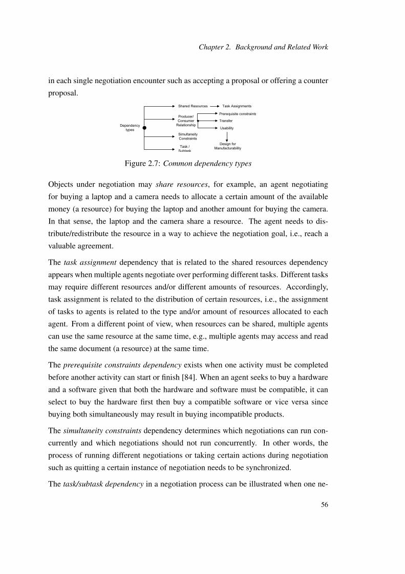
Chapter 2. Background and Related Work
in each single negotiation encounter such as accepting a proposal or offering a counter
proposal.
Figure 2.7: Common dependency types
Objects under negotiation may share resources, for example, an agent negotiating
for buying a laptop and a camera needs to allocate a certain amount of the available
money (a resource) for buying the laptop and another amount for buying the camera.
In that sense, the laptop and the camera share a resource. The agent needs to dis-
tribute/redistribute the resource in a way to achieve the negotiation goal, i.e., reach a
valuable agreement.
The task assignment dependency that is related to the shared resources dependency
appears when multiple agents negotiate over performing different tasks. Different tasks
may require different resources and/or different amounts of resources. Accordingly,
task assignment is related to the distribution of certain resources, i.e., the assignment
of tasks to agents is related to the type and/or amount of resources allocated to each
agent. From a different point of view, when resources can be shared, multiple agents
can use the same resource at the same time, e.g., multiple agents may access and read
the same document (a resource) at the same time.
The prerequisite constraints dependency exists when one activity must be completed
before another activity can start or finish [84]. When an agent seeks to buy a hardware
and a software given that both the hardware and software must be compatible, it can
select to buy the hardware first then buy a compatible software or vice versa since
buying both simultaneously may result in buying incompatible products.
The simultaneity constraints dependency determines which negotiations can run con-
currently and which negotiations should not run concurrently. In other words, the
process of running different negotiations or taking certain actions during negotiation
such as quitting a certain instance of negotiation needs to be synchronized.
The task/subtask dependency in a negotiation process can be illustrated when one ne-
56
2.4. Dependencies and Coordination
gotiation depends on some other negotiations, i.e., the negotiations are multi-linked
[165]. For example, if there are 3 negotiations a, b, c, but negotiation a depends on
negotiations b and c (i.e., negotiation a is successful iff negotiation a is successful
and both negotiations b and c are also successful), then we consider that negotiation a
has two subtasks (i.e., b and c).
One of the most complicated activities during negotiation is deciding on the value of
the next proposal by an agent. During negotiation and for each negotiation round,
an agent needs to select a bidding strategy that can generate the next proposal, i.e.,
generate an offer or a counteroffer. Calculating the value of an offer/counteroffer in
each negotiation round is a non-trivial process due to the following:
• the process can be affected by the actions of the outside options
• the interdependency between the issues of the same object
• the interdependency between the issues of different objects
• the interdependency between different negotiation objects.
In the next next two sections, there will be more elaboration on the interdependency in
the one-to-many negotiation considering the dependency from the point of view of a
buyer agent negotiating concurrently with multiple seller agents.
2.4.1 Interdependency Amongst Objects
Sometimes, it it important to procure a certain number of objects in a certain order
when the objects are interdependent. The interdependency between objects results
from the precedence relation between the objects. For example, hardware and software
objects can be interdependent due to the compatibility issues between softwares and
hardwares. In many cases, software needs to run on compatible hardware and hardware
has some requirements for the software it can operate. In this case, procuring the
hardware first has an effect on the type of software that is going to be procured and vice
versa. Solving the problem of procuring different objects with precedence constraints
can be solved either by sequential negotiation or by concurrent negotiation.
57

Chapter 2. Background and Related Work
Accepting a number of agreements by an agent in a certain order while negotiating
concurrently with multiple opponents is equivalent to achieving the same number of
objects in the same order while negotiating with opponents sequentially. Procuring a
certain number of objects sequentially is the easiest solution to solve the problem of
procuring a certain number of objects in a certain predefined order. However, using the
sequential approach has a few drawbacks. Firstly, because negotiations are conducted
once at a time, it is difficult to predict the results of the future negotiations in terms of:
1) whether a certain negotiation instance will be able to reach an agreement 2) the ex-
pected utility of the agreements. Secondly, it is difficult to allocate resources for each
negotiation instance because we have no knowledge about the demand behavior of the
opponents of the future negotiations. For example, we might allocate more resources
for the first few negotiation instances to guarantee reaching agreements but the re-
sources for the next negotiations may not be enough to guarantee reaching agreements
over the rest of the objects. Finally, the sequential approach takes more time.
An alternative solution to the sequential negotiation approach is adopting the concur-
rent negotiation approach where a negotiating agent receives feedback during negoti-
ation in terms of the opponents’ offers and can act accordingly to fine tune its strat-
egy and resource allocation pattern. The drawback of the concurrent approach is the
need for coordination whenever any type an of interdependency exists between objects
or between objects’ issues, etc. For example, different objects may have interdepen-
dency between their attributes such as interface compatibility between two different
softwares. Sometimes buying object (o1) before buying object (o2) causes a loss in
utility such as confirming a hotel reservation before confirming a flight. If the flight is
canceled for any reason then the buyer might be obliged to fulfill his/her obligations
towards the hotel reservation.
In some cases, the order of procurement is not defined before the start of negotiation,
it could be determined dynamically during negotiation. For example, a person needs
to book a flight and an accommodation before starting his/her vacation and at the same
time, he/she does not know which one is more difficult to find. During negotiation, the
agent working on the behalf of that person detects which one is more difficult to secure
and decides the order of agreements and resource allocation dynamically. The agent
may find that booking a flight is more difficult than booking an accommodation, then
it decides to secure an agreement for booking the flight first.
58

2.4. Dependencies and Coordination
2.4.2 Interdependency Amongst Issues
Each object under negotiation is characterized by one or more negotiation issues or
attributes. The interdependency between two (or more) issues results from existing
relations between them in the sense that the utility of an agreement on the two issues
together is greater than the sum of the utilities if the two agreements are achieved in
disjunct manner. This type of interdependence is called preferential dependency [92]
since the utility of an issue depend on the value of one or more issues. For example, a
flight can have two issues, the day-of-the-flight and the time-of-the-flight. Assume that
a certain passenger prefers to fly on Friday before 12PM. The travel agency says there
is a flight available on Thursday before 12PM and another one is available on Friday
after 5PM. To evaluate the situation, the utility of flying on Friday before 12PM is
more than the sum of the utilities of flying on Thursday before 12PM and the utility of
flying on Friday after 5PM. This type of relation between the issues of day-of-the-flight
and time-of-the-flight is called complementary relation, i.e., the issues complement one
another. Moreover, different issues can be interdependent in terms of their acceptable
values. For example, an agent may agree to pay a high price for a high quality product.
When the number of negotiation issues is large, it becomes difficult to search for a
proper combination between the values of issues since the search space becomes large.
When the issues are of a continuous type, the search problem becomes even more
difficult and intractable. Utility functions without preferential dependencies have a
simple linear structure (weighted average) with a single optimum value. On the other
hand, utility functions with preferential dependencies often have a nonlinear behavior
with multiple optima structure.
Apart from dealing with the problem of searching for the best offer that can achieve
the highest possible utility in case the utility function is nonlinear, we focus on the
problem of allocating shared resources amongst different negotiation issues. In many
cases, the distinct objects can have the same issue such as price. In our work, we call
the issues of different objects that share the same resource as common issues.
Definition 2.5. (Common negotiation issue)
A common negotiation issue is an issue ji ∈ J s.t. at least two subsets Jk, Jl ∈ 2J exist
where ji ∈ Jk ∩ Jl. J is the set of negotiation issues.
59

Chapter 2. Background and Related Work
In other words, a common issue is an issue that is common amongst multiple objects.
For example, multiple services can have the price issue as a common issue.
To this end, we propose managing resources shared amongst common issues as an
approach for coordinating the bidding strategy which takes into consideration the be-
haviors of the opponents over the common issues, see Section 4.3. Managing the distri-
bution of the available resources (which is part of the bidding strategy) is one solution
for managing the interdependency problem.
2.5 Coordination and Negotiation
Negotiation is a potential mechanism for agents to use for coordinating their actions.
A possible classification of coordination types is shown in Figure 2.8. In the cen-
tralized coordination, all agents report to a central authority that make decisions by
looking at the coordination problem globally. The main drawbacks of the centralized
coordination are the single point of failure and the trust problems. The single point
of failure means that if the central authority fails, the entire system will stop working.
In a community of heterogeneous agents, it is difficult to apply the centralized coordi-
nation approach since agents can have different and conflicting goals and agents find
it difficult to have a trust in a third party to coordinate their actions. The hierarchy
coordination is similar to the centralized coordination except that in hierarchy coordi-
nation, there are different levels in the decision making process and each level needs
to report to the upper level and different levels in the hierarchy can be responsible for
different types of decisions. Ossowski and Menezes [110] present the term emergence
coordination which indicates that the solutions to the coordination problems emerge
from the interaction between agents (or processes) in which an agent tells the other
agents about its actions without expecting a direct consequence from that interaction.
Such coordination mechanisms can be efficient in particular games such as the mi-
nority game [8]. However, negotiating agents are affected directly by the messages
(proposals) exchanged between them.
In multiagent systems, the focus is on the decentralized coordination. The decentral-
ized coordination is a more interesting approach since it does not have the drawbacks
inherited in the centralized coordination approaches. In addition, agents can be more
60
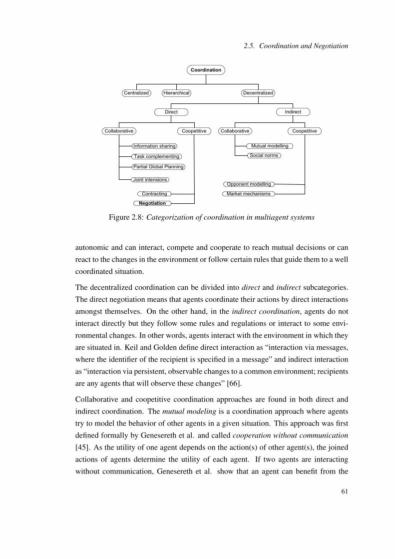
2.5. Coordination and Negotiation
Figure 2.8: Categorization of coordination in multiagent systems
autonomic and can interact, compete and cooperate to reach mutual decisions or can
react to the changes in the environment or follow certain rules that guide them to a well
coordinated situation.
The decentralized coordination can be divided into direct and indirect subcategories.
The direct negotiation means that agents coordinate their actions by direct interactions
amongst themselves. On the other hand, in the indirect coordination, agents do not
interact directly but they follow some rules and regulations or interact to some envi-
ronmental changes. In other words, agents interact with the environment in which they
are situated in. Keil and Golden define direct interaction as “interaction via messages,
where the identifier of the recipient is specified in a message” and indirect interaction
as “interaction via persistent, observable changes to a common environment; recipients
are any agents that will observe these changes” [66].
Collaborative and coopetitive coordination approaches are found in both direct and
indirect coordination. The mutual modeling is a coordination approach where agents
try to model the behavior of other agents in a given situation. This approach was first
defined formally by Genesereth et al. and called cooperation without communication
[45]. As the utility of one agent depends on the action(s) of other agent(s), the joined
actions of agents determine the utility of each agent. If two agents are interacting
without communication, Genesereth et al. show that an agent can benefit from the
61

Chapter 2. Background and Related Work
information gathered about its opponent by determining its rational action(s) and act-
ing accordingly [45]. If the aim of the agents is to achieve a common goal the mutual
modeling is the name of the approach. If agents have different goals, then the opponent
modeling is the name of the coordination approach which is similar to the mutual mod-
eling except that the mutual modeling is used in a totally collaborative environment.
Market mechanisms can involve both cooperative and competitive behaviors.
The social norms is another collaborative coordination approach where agents adhere
to some norms (which are established or expected) during the interaction. For example,
it is a social norm for a student to raise his/her hand before asking a question while in
a class. On the other hand conventions or social laws can be either designed offline or
emerge from within the system. For more information about emergence from within
the system social laws, see [158].
The information sharing is a collaborative coordination approach where agents share
information and try to coordinate their tasks accordingly. For example, a set of agents
can share and exchange information about each others skills and expertise before as-
signing a certain set of tasks. In task complementing, agents collaborate in the process
of task assignment in a complementary fashion where agents are assigned task(s) in
which their expected performance is high. Factors like an agent’s resources and the
expertise of each agent are taken into consideration in the process of task assignment.
The partial global planning (PGP) is a distributed control technique to ensure that the
local plan of each node in a network is coherent with the local plans of the neighbouring
nodes assuming that each node in the network represents an agent [29]. It is called
partial because agents do not aim to generate a plan for the whole system and it is
called global because agents exchange local plans to form non-local plans. The partial
global planning consists of three repetitive steps: 1) each agent generates short-term
plans that aim to achieve a predefined goal(s) 2) agents exchange information that help
in updating their short-term plans 3) agents modify their short-term plans. The PGP is
extended into generalized partial global planning that makes use of five techniques to
coordinate agents’ activities: Updating non-local viewpoints, communicating results,
handling simple redundancy, handling hard coordination relationships and handling
soft coordination relationships [25][159].
The joint intention coordination is a technique that considers the intentions of agents
in terms of their planning doing certain work. Intentions can provide stability, pre-
62

2.5. Coordination and Negotiation
dictability, flexibility and reactivity. The first two points are important for the social
interaction while the latter two points are important to cope with a changing environ-
ment [159]. Jennings developed and implemented the joint responsibility coordination
model that is based on joint intentions. Before commencing the joint problem solving
process, the defined preconditions must be satisfied. The joint responsibility model as-
sumes that each individual within a system needs to stay committed to using the agreed
upon solution to achieve the common goal until one of a set of events is fired, such as
the objective has been met, the objective will never be met etc. If a team member agent
decides to decommit its responsibility, it must ensure that all of its team members are
aware of the new status to enable the rest of the team to reassess the new situation
and judge the viability of the joint action especially the actions that are supposed to be
carried out by the decommitted team member [56].
The contracting is a coordination method that can apply in a situation where a group
of agents compete for a certain number of tasks. The Contract Net (CNET) protocol
is “a high level protocol for communication among the nodes in a distributed problem
solver” [142]. To apply the CNET protocol as a task allocation mechanism amongst a
group of agents, tasks are announced by a manager agent. Then each group member
bids for one or more tasks, and finally the manager allocates tasks. The agents who are
selected to perform tasks are called contractors. Each contractor agent sends a report to
the manager after the completion of its allocated task(s). It is possible for a contractor
agent to subdivide its tasks and play the role of a manager by announcing the new
subdivided tasks. An agent’s decision to bid on new tasks depends on the marginal
cost calculations. If the marginal (extra) cost is less than or equal to zero, then it is
rational for the agent to bid on the new tasks, otherwise it is not rational to bid on the
new tasks since the agent would need more resources to complete the new bids than
what it has. This protocol was inspired from the way that organizations usually put
contracts out to tender [159].
As shown in Figure 2.8, negotiation is considered a coopetitive, direct and decentral-
ized coordination mechanism. Negotiation is coopetitive because agents can compete
and cooperate during negotiation. For example, agents cooperate when they use the
trade-off negotiation mechanism to reach an agreement and compete when they need
to concede to reach an agreement. Negotiation can be direct when agents interact
with each other directly without any mediation mechanism. It is decentralized since
63

Chapter 2. Background and Related Work
agents synchronize their actions by interacting with each other without a central deci-
sion making authority. In other words, the decision making mechanism is distributed
since each agent can participate in reaching the final agreement(s).
The relationship between negotiation and coordination is presented from a new angle
here. Negotiation is listed as one mechanism in which agents can use to coordinate
their actions, see Figure 2.8. This thesis considers a buyer agent negotiating concur-
rently with multiple seller agents and since the buyer agent is interacting with multiple
agents concurrently, its actions need to be coordinated to achieve the overall goal of
negotiation. During negotiation, the buyer agent receives multiple offers from a group
of seller agents. Consequently, it needs to decide how to react to each agent since the
different negotiation instances (see Section 3.2) can be interdependent. For example,
when the buyer agent receives 4 different offers simultaneously, it can accept the best
one of them and quit negotiation. On the other hand, there is a possibility for the
buyer agent to receive a better offer from other agent(s) if it stays in negotiation. The
buyer agent can monitor the level of concessions offered by each agent by inspecting
the current negotiation threads and deciding what to do next. For example, when the
behaviors of the seller agents vary, this can be a favorable situation to the buyer agent
since it means the chance for receiving a better offer in the future is high. It can be
concluded from this example that different negotiation instances can be interdependent
from this point of view. In addition, Section 2.4 discusses possible dependency types
in negotiation. One of the important dependency types that is investigated in this thesis
is when one or more issues of different objects share a resource. For more detail on the
coordination problem in one-to-many concurrent negotiation, see Chapter 4.
Since the focus of this thesis is on the bidding (bargaining) strategies in the one-to-
many interaction where a buyer agent is negotiating concurrently with a set of seller
agents over one or more negotiation objects, the following few sections discuss the
related work and present and analyze different negotiation strategies that are proposed
in the literature to coordinate the one-to-many negotiation.
The sections are divided according to the number of negotiation issues and/or a number
of negotiation objects under negotiation. This division is chosen to facilitate the pre-
sentation of the related work since the number of negotiation issues and/or the number
of negotiation objects have an effect on choosing a certain negotiation strategy. For
example, if agents are negotiating over a single issue, then the trade-off negotiation
64
2.5. Coordination and Negotiation
tactic is not an option. When agents are negotiating over multiple objects, the issues
of the objects may share a resource in which the allocation of that resource needs to be
coordinated dynamically during negotiation.
2.5.1 One-to-Many Negotiation Over a Single Issue
In the context of business negotiation, the single issue negotiation is the most inves-
tigated type of negotiations where in most cases the single issue represents the price
issue. This section discusses various methods proposed in the literature concerning the
one-to-many negotiation over a single continuous issue.
In their proposed one-to-many negotiation model, Rahwan et al. [115] propose four
coordination decision making mechanisms for a buyer agent negotiating with multiple
seller agents concurrently: 1) desperate strategy in which the buyer agent accepts the
first acceptable agreement and quits negotiations with all other sellers, hence it is called
desperate 2) patient strategy where the buyer agent makes temporary agreements with
some of the seller agents during negotiation and holds on to these agreements until all
the remaining instances of negotiations are finished, then the buyer agent selects the
agreement with the highest utility and renege from all other agreements 3) optimized
patient strategy is similar to the patient strategy except that it does not accept a new
agreement with less utility than the highest acceptable one 4) manipulation strategies
in which the coordinator entity in the buyer agent changes the negotiation strategies of
its sub-negotiators during negotiation. Changing a negotiation strategy means adapting
one or more of the negotiation strategy parameters, see Chapter 4.
The first three strategies (i.e., desperate, patient and optimized patient) assume that the
buyer agent has the privilege of reneging on temporary agreements without penalty.
This assumption can be realistic in situations where the number of seller agents is
large and/or the seller agents are offering infinite supply, e.g., information. In such
cases, a seller agent might be satisfied to make deals with many potential buyers in
hope that some of the buyers will confirm their deals later. The other two agreement
handling rules are: an agent can renege from an agreement and incur a penalty to be
paid, the second one is that an gent must honor its agreement(s) which means an agent
must be committed to executing its agreement(s).
If reneging on an agreement incurs a penalty, the processes of deciding to make a
65

Chapter 2. Background and Related Work
temporary agreement and reneging on agreement needs to be analyzed carefully. In
other words, a commitments/decommitment mechanism is required. A rational agent
can only renege on a temporary agreement if and only if the utility of the new agree-
ment(s) is larger than the utility of the temporary agreement plus the incurred reneging
penalty. The amount of penalty can be either a fixed amount that is agreed upon by
negotiation partners or dynamically calculated according to a certain formula. Empir-
ical results show that when agents use a dynamic method to calculate the amount of
incurred penalty, they can be more flexible in deliberating about their behaviors that
results in gaining a better negotiation outcomes than using a fixed amount [105].
Managing commitments in concurrent negotiation is investigated in the literature, e.g.,
[105][2]. Nguyen and Jennings [105] propose a commitment model that considers
calculating the amount of penalty according to equation 2.14.
ρ(t)d = U(xtss→d
)×(ρo +
t− tstdmax − ts
× (ρmax − ρo)), (2.14)
where ρ(t)d is the penalty fee that has to be paid by the agent d at time t, U s(xtss→d
)
is the utility value of the offer xtss→d
calculated according the utility function of the
agent d, ρo is the fee that needs to be paid if the deal is broken at the contract time
(ts). Finally, ρmax is the fee that needs to paid if the deal is broken at the execution
time which is considered the agent’s d deadline. It is a common sense that if an agent
breaks a deal at the execution time, the harm to the contractee agent is maximum and
so the penalty fee should be. According to equation 2.14, the penalty is maximized if
an agent breaks a deal at its deadline. The agent d may commit (accept) a new offer
and renege on an existing offer (if it exists) if U(xts′→d
) > U(xt′
s→d) + ρ(t)d, t > t
′
and the degree of acceptance for the offer xtss′→d
is higher than a certain predefined
threshold. Even though the model of calculating the penalty fee is a dynamic since it
takes into consideration the time elapsed, it is not clear that how genuine an agent can
be in declaring its U s(xtss→d
) value since the preference over an outcome is considered
a private information. In addition, it is not clear how an agent can determine the value
of the threshold.
In their work, An et al. [2] consider the problem of resource allocation in a dynamic
environment like the cloud computing platforms and propose a negotiation mecha-
nism where agents negotiate over a price of a resource and a decommitment penalty of
66

2.5. Coordination and Negotiation
reneging on a contract. The rule proposed to determine the decommitment penalty is:
The lower the price, the higher the penalty. This rule can be a practical one. For exam-
ple, a seller may agree to offer a resource with a low price in exchange for receiving
a high penalty fee if the buyer agent decides to renege on the agreement. In this way,
the seller agent either sells its resource or receives a good payment from the buyer in
case it reneges on the agreement. When a buyer agent needs a set of resources and no
one seller agent can fulfill its demand, the experimental results show that the optimum
strategy for the buyer agent is to make two sets of agreements. A possible reason is
that the buyer agent needs to pay larger penalty fees when it makes more agreements
since it needs to confirm one set of agreements and decommit all other agreements at
its deadline. On the other hand, if the buyer agent makes one agreement, some seller
agents may decommit some agreements and the buyer agent will not be able to com-
plete its tasks because of shortages in resources. For more information on commitment
management in automated negotiation see [129] [136].
This thesis does not consider the negotiation situation where agents incur a penalty
when reneging on temporary deals. However, it does consider managing the negoti-
ation strategy for the other two agreement rules: firstly, an agent has the privilege to
decommit an agreement without incurring a penalty. Secondly, the agents must honor
their agreements. Even though giving an agent the right to decommit a previously
agreed upon contract (with penalty) would give more flexibility to the agent to adapt
to the new changes in the environment, the other agreement rules are more common in
the literature.
The outside options in the multi-bilateral negotiation can affect the negotiation strat-
egy of an agent because of the possible interdependent relationships amongst different
negotiation instances as discussed earlier. To study such interdependencies, Li et al.
investigate the effect of outside options on the negotiation strategy of a buyer agent
negotiating concurrently with multiple seller agents where the agreements are consid-
ered binding to the negotiating agents [23]. Knowledge of an opponent’s reservation
value on an issue such as price can change the mental state of an agent which results in
changing its negotiation strategy by changing its reservation price towards a higher util-
ity reservation price. The objective for the buyer agent is to achieve a single agreement
with the highest possible utility. The important parts of the study consider the one-
to-many negotiation and investigate two situations: the first situation is when a buyer
67

Chapter 2. Background and Related Work
agent is negotiating concurrently with a number of seller agents and new seller agents
are not expected to join negotiation. In this case, the buyer agent has a number of nego-
tiation threads equal to the number of seller agents. In this case, the buyer agent assigns
to each thread a reservation utility value equal to the expected utility from the multi-
threaded negotiation formed by all other threads. From one thread’s perspective, all
other threads are considered outside options and form a synchronized multi-threaded
negotiation. The study proposes four heuristics to estimate the expected utility from
a synchronized multi-threaded negotiation. Three of them (conservative estimation,
medium estimation and uniform approximation) use the reverse English auction the-
oretical analysis results in the approximation process for the expected utility in the
synchronized multi-threaded negotiation. The proposed mechanisms are based on the
assumption that the buyer agent has a prior belief about the probability distribution of
each seller agent’s reservation price. The fourth mechanism is a learning mechanism
that depends on the outcomes of previous negotiations. The study assumes that the
data comes from the market survey or from data of a third party. The proposed learn-
ing mechanism approximates the expected utility from a multi-threaded negotiation by
estimating the expected utility from the most competitive thread in a single negotiation.
For more detail, see [23].
The second situation is the dynamic multi-threaded negotiation where the buyer agent
is negotiating concurrently with multiple sellers and more seller agents are expected
to join the current negotiation. In that case, the bargaining power of the buyer agent
becomes better. The outside options for a negotiation thread in this case includes
both, the current outside options and the negotiation threads that can be initiated in
the future by the new arrived sellers. The arrival pattern of the outside options is
assumed to follow a Poisson process. The assumption about the arrival probability
along with the probability distribution about the opponents’ values that are expected
to arrive in the future are used by the buyer agent to forecast the number and the
quality of the outside options arriving. The work presented in [23] demonstrates how
multiple negotiation instances can be interdependent. The drawback of the described
work is in the previous knowledge assumption about the probability distribution about
the opponents’ reservation prices and about the value of the seller agents that might
join the current negotiation which are necessary for the described approaches. In open
and dynamic automated negotiation systems, such knowledge is difficult to attain.
68
2.5. Coordination and Negotiation
The Markov chain model is proposed as a decision making mechanism in the one-
to-many negotiation where a buyer agent is negotiating with multiple seller agents
concurrently and the agreements are considered binding to agents. An et al. propose a
decision making strategy based on Markov chain model (Markov chain based decision
making MCDM) of a negotiation process [3]. The MCDM considers the dynamics and
uncertainties of the negotiation process using stochastic modeling of the negotiation
process. The aim of the MCDM mechanism, at each negotiation round, is to decide
whether to accept the best available offer and quit negotiation or to proceed with nego-
tiation for the hope that the buyer agent would receive an offer(s) with better value(s).
Again, the study presents a model that captures the interdependencies amongst the ne-
gotiation instances or threads. In their work, An et al. consider the price issue as the
only negotiation issue. The limitation of the proposed approach is in its assumption
that all agents use the set-and-wait negotiation tactic.
In the case an agent uses the time-dependent tactics, limβ→∞ α(t) = (t/tmax)β =
0 where 0 ≤ t < tmax and limβ→∞α(t) = (t/tmax)β = 1 where t = tmax, see Equa-
tion 2.3. When an agent uses very large β value it offers its initial value at the start of
negotiation and waits (set-and-wait strategy) until its deadline approaches and offers
its reservation value. The MCDM approach assumes that the buyer agent offers a very
low price and the seller agents offer a very high price at the beginning of negotiation.
Even though the set-and-wait strategy is proven [137] to be the dominant strategy for
an agent using a time-dependent strategy regardless of the type of negotiation stra-
tegies its negotiation partners may use, this assumption does not fulfill some of the
automated negotiation objectives where agents are supposed to exchange multiple of-
fers and counteroffers in order to broaden the search space for possible agreements that
suit the negotiating partners. The negotiation strategies proposed in this thesis assume
that agents exchange multiple offers and counteroffers during a negotiation encounter.
A coordination model that is based on categorizing the types of the opponent agents
into either conceder or non-conceder are proposed for a buyer agent negotiating con-
currently with multiple seller agents. The buyer agent is assumed to have the privilege
of making temporary agreements without the need to pay a penalty fee in case it re-
neges on an agreement(s). In their proposed model, Nguyen and Jennings assume that
the buyer agent has a probability distribution about the types of agents (i.e., conceder
type and non-conceder type) taken from previous negotiations or from any other party
69

Chapter 2. Background and Related Work
[106]. If no information is available about the types of seller agents , then all seller
agents are considered of unknown type. The model also uses the percentage of success
(PS) matrix and the pay off (PO) matrix. The PS records the rate of reaching a suc-
cessful agreement for each type of the buyer agent’s strategies against the two types
of seller agents. In other words, the rows of the PS matrix consist the buyer’s strate-
gies (conceder, linear and tough) and the columns are the conceder and non-conceder
seller agent types. The PO is similar to the PS matrix except it records the utility rate.
Equation 2.15 finds the buyers’ expected utility of using a certain strategy λ where
λ ∈ conceder, linear, tough which are the only strategies that the buyer uses in the
proposed model.
EU(λ) =∑
s∈Atypes
PS(λ, a)PO(λ, a)P (a), (2.15)
where P (a) is the probability that the seller agent is of type a. The values PS(λ, a)
and PO(λ, a) are taken from the matrices PS and PO at the intersection of λ and
a. The buyer agent calculates three EU(.) values, one expected utility per a strategy
λ ∈ conceder, linear, tough. The buyer agent selects the strategy with the highest
expected value. That process is repeated to select a strategy for each negotiation thread.
The model uses Bayesian rule to update the probability distribution of the agent types
and continues on to select a strategy for the second thread. The experimental results
show that the initial information about the probability distribution of the seller types
have small positive (1-2 %) results on the buyer’s utility rate. Most of the positive
experimental results are due to the reclassification process of the seller agent types that
the buyer agent performs during negotiation. The buyer agent assigns a certain seller
agent into either theAcon or theAnon sets according to the utility value of its proposals.
The buyer agent starts classifying seller agents after receieving the third proposal as
follow: at time t = 3 and if( U(s, t)− U(s, t− 1)
U(s, t− 1)− U(s, t− 2)> ψ
)then the seller agent
s ∈ Acon otherwise s ∈ Anon where ψ is the threshold value set on the concessionary
behaviour. The buyer applies this procedure in each negotiation round. Equation 2.15
is used to select a strategy λ accordingly. In this case the P (s) can be either 1 or 0.
The proposed model is compared with the desperate, the patient and the optimized
patient strategies that were discussed earlier. The experimental results show that the
proposed model outperforms the mentioned strategies in terms of the utility rate and
70

2.5. Coordination and Negotiation
agreement rate. However, the model still needs the PO and the PS matrices for the
strategy selection process. In addition, the model limits the buyer’s negotiation tactics
into only three tactics which is a bit restricting since the number of negotiation tactics
can be large. Even though it is mentioned in the experimental section that the number
of negotiation issues considered in the experiments can be between 1 and 8, the real
impact of having multiple negotiation issues is not clear since the model classifies the
seller agents according to the utility of the last 3 offers received from each seller. In
addition, the buyer agent uses the time-dependent tactics which -without manipulation-
concede on all issues with the same rate in each negotiation round. Moreover, it is not
clear how the ψ threshold value can be set and whether it is a fixed value or can be
changed during negotiation.
Finally, another study proposes manipulating the convexity of the concession curves of
a buyer’s agent is presented in [90]. The proposed method uses the current behaviors
of the current seller agents to adapt the slop of the buyers’ concession curves during
negotiation.
2.5.2 One-to-Many Negotiation Over Multiple Issues
In real life, most negotiations involve more than one issue. For example, buying a
laptop may involve negotiating the price of the laptop and both, the memory size and
processor speed. If the agents participating in negotiation are competitive and self
interested, then the objective of each agent is to reach an agreement with the highest
possible utility regardless of the opponents’ needs or preferences. However, when
negotiation involves multiple issues, agents usually have divergent preferences over
different issues which allows them to reach an efficient agreement for both parties, i.e.,
achieving a win-win outcome.
There are a fair number of research papers that discuss negotiation over multiple is-
sues, e.g., [34][37]. However, most works consider bilateral negotiation. For exam-
ple, Fatima et al. propose a negotiation model for multi-issue negotiation under time
constraints in an incomplete information setting [37]. The proposed model allows ne-
gotiation over one or more negotiation objects where each object is characterized by a
single continuous issue. Moreover, the model investigates the scenario where agents
negotiate over a single object characterized by multiple issues. However, the work in-
71

Chapter 2. Background and Related Work
vestigated in [37] focuses on the problem of the agreements’ implementation scheme in
which the agreements can be implemented either sequentially or simultaneously. The
work of this thesis focuses on developing dynamic negotiation strategies that can guar-
antee effective and/or efficient outcomes for a buyer agent negotiating concurrently
with multiple seller agents.
In an interesting study about the one-to-many multi-attribute negotiation setting, Van
de Walle et al. [151] consider the problem of evaluating and ranking different offers
proposed by a set of buyers. The negotiation setting involves a seller negotiating with
multiple buyers over a single object characterized by multiple issues. Given the re-
ceived offers from the buyers, the objective of the study is on which buyer the seller
should focus on to negotiate further and sell its product. A simple strategy to answer
such a question is to rank the buyers according to the value of their offers. In this case,
the value of each offer is reduced to a single number, i.e., the weighted average utility
of the offer. Van de Walle et al. propose an alternative strategy that preserves the infor-
mation richness of an offer by doing pairwise comparisons of the seller’s preference on
the buyers’ offers and rank the buyers (a partial order ranking) accordingly. The pro-
posed ranking strategy is based on the fact that the preferences over negotiation issues
may vary by different negotiating partners. The proposed approach uses the fuzzy sets
and fuzzy relations in the pairwise comparison between different issues. In a fuzzy
quasi-order relation, each α-cut is a crisp quasi-order relation. Each α-cut of a fuzzy
quasi-order relation is a quasi-order relation in the set of buyers. The equivalence re-
lation partitions the buyers into equivalence classes of buyers in which the buyers of
each class are of equal quality to the seller agent. The same study also analyzes the
sellers’ preferences over its different attributes or issues and compares between them
at different α-cuts.
The first step in implementing the proposed approach is to construct the preference
relation matrix. To construct the matrix, the seller needs to assign a value (usually
between 0 and 1) to each proposed value for each issue in the received offer of each
buyer. For example, if a buyer proposes $10 and 2 days delivery time over a certain
item and the preference of the seller is $15 and 2 days delivery time, the seller agent
may assign 0.4 to the received price value and 0 to the received delivery time value. It
means that the seller does not prefer more than the value of the offered delivery time
while the value of the received price is less than its expectation, hence the number
72

2.5. Coordination and Negotiation
corresponds to the received price in the preference relation matrix and is estimated to
be 0.4. Building such a matrix is subjective and is not easy to start with. In automated
negotiation, the process of constructing the preference relation matrix needs to be re-
peated each time the seller agent receives a new set of offers. It is not clear how to
automate building such matrix during negotiation by an agent. Further more, giving
the analyses of buyers’ responses and seller’s preferences, the study does not show how
the seller would choose the level of α-cut. Finally, the proposed work does not explain
how to respond to each buyer using the information about buyers’ classification.
In another study, Gerding et al. [46] investigate the negotiation scenario where a seller
agent is negotiating concurrently with multiple buyer agents for the purpose of selling
unlimited amounts of goods such as information. The study proposes a number of
one-to-many bargaining strategies for the seller agent that takes into consideration the
fairness amongst different buyers. The fairness can be defined from either the seller
agent’s point of view or from a buyer agent’s point of view. Assume that a buyer
reaches an agreement at time td ∈ [ts, ts + ∆], ds is a start time. This agreement
is fair relative to a fixed interval ∆ > 0 if the seller agent is indifferent amongst all
other agreement reached within the interval [ts, ts + ∆]. Its definition from a buyer’s
point of view is related to the notion of envy-free auctions presented in [49]. If a
deal reached at td ∈ [ts, ts + ∆] and a buyer does not strictly prefer any other deal
reach within the interval [ts, ts + ∆], the deal is considered fair. The proposed idea of
assuring fairness is that the seller agent should not accept two simultaneous (or within
a predefined slot of time) proposals from two different buyers or more if the proposals
differ in their utilities. To be fair amongst buyers, the seller agent should be indifferent
to all proposals within a certain slot of time. The action of the seller agent in that case
is to propose a counteroffer(s) that ensures equality amongst offers within a certain
predefined time interval.
In dynamic and competitive environments, we do not expect buyers to communicate
their agreed upon deals given that each buyer agent accepts an agreement according
to its own constraints. In addition, the experimental results are based on using an
evolutionary algorithm that allows agents to learn from previous negotiations. Again,
dynamic agents in dynamic environments may not repeat their behavior patterns which
makes using an evolutionary algorithms of little use here.
In another study which also considers a seller agent negotiating with a number of
73

Chapter 2. Background and Related Work
buyer agents for selling bundles of news items where each news item is characterized
by negotiation issues: price, quality and content of the delivered goods, Somefun et al.
[143] propose an approach where the seller agent uses both, concession strategies and
Pareto efficient search strategies during negotiation. The study considers also reaching
agreements that are fair to the customers. In their market model, the news items are
divided into a number of categories. Within each category, there are two quality of
service levels. The first level (low quality) shows the headline news only, while the
second one (high quality) offers the complete article. The customer bargains with the
seller over the bundle tariff which consists of a fixed part (pf ) and a variable part,
pv. The pf is the price specified to a bundle with a certain quality of service while
the pf is the price the customer pays for reading a full article whenever the quality
of service specifies delivering only the article headline. For each information bundle,
agents negotiate over the pv and pf . The idea used to achieve a fair agreement with a
buyer agent is similar to the idea implemented in [46].
In addition, the study [143] proposes the orthogonal and orthogonal-DF mechanisms
as two Pareto efficient search strategies. An agent using the orthogonal strategy finds
a counteroffer (at time t + 1) that is closest (measured in Euclidean distance) to the
last received offer that has the same utility as the one generated at time t − 1. The
orthogonal-DF adjusts the value of one negotiation issue (e.g., pv) that was generated
by the orthogonal mechanism to speed up the search and its accuracy. Consequently,
the pf also needs to be changed to keep the agent on its current iso-curve. The best
results in terms of the distance from the Pareto efficient solution is when a buyer agent
uses the orthogonal technique and the seller agent uses the orthogonal-DF technique.
If both use the orthogonal-DF, the results are similar to the results when agents use
random search. It is obvious that none of the agents have an advantage over the other
if both are using the same strategy.
The proposed Pareto efficient search mechanisms are limited to the situation where
two continuous issues are used. In addition, it is not clear when the seller agent should
move from one iso-curve to another during negotiation. Moreover, the approaches
assume that the seller agent decreases its aspiration level by a fixed amount each round.
However, the number of existing buyer agents and their behaviors are not considered
as a factor that can affect the amount of the next aspiration level!
As a means to approximate a version of qualitative Vickrey auction (QVA) that pro-
74

2.5. Coordination and Negotiation
duces a Pareto-efficient outcome where the best seller wins, Hindriks et al. [54] pro-
pose using one-to-many negotiation where a buyer agent negotiates with multiple seller
agents over an object characterized by multiple issues. The reason behind using the
one-to-many negotiation is that at least one negotiation party needs to disclose its pref-
erences and in many cases that option is not accepted by any party due to privacy and
trust concerns. Three variants of the alternating protocol are analyzed: 1) the set of
allowed offers for all agents is restricted 2) the winning offer is announced after each
round 3) the sellers are told whether they have won or not after every round. The re-
sults of the experiments show that each of the three mechanisms is able to approximate
the efficient outcome defined by the QVA [54]. The interesting results of this work
indicates that the one-to-many negotiation over multiple issues can reach efficient out-
comes that are similar to the one obtained by the QVA without the need from any agent
to disclose its preferences.
As a dynamic negotiation strategy, a meta-strategy that uses two different offer gener-
ation tactics is proposed in [87]. The strategy uses a concession tactic and a trade-off
tactic. In each negotiation round, the buyer agent needs to select which tactic type to
use depending on the current behaviors of the opponents in terms of their concessions.
During negotiation, the buyer agent assigns each seller agent to either a favorable group
or unfavorable group. The favorable group offers more concessions than the conces-
sions offered by the corresponding buyer agent’s delegates.
2.5.3 One-to-Many Negotiation Over Multiple Distinct Objects
The problem of procuring multiple distinct objects concurrently is a difficult problem
due to the possible interdependencies amongst negotiation objects from one side and
amongst negotiation issues from the other, see Section 2.4.
As a resource coallocation procurement one-to-many negotiation based model was
proposed as a GRID resource management system. In their model, Sim and Shi [138]
consider a buyer agent seeking to procure multiple distinct services, each characterized
by the price as the only negotiation issue. For each service, the buyer agent conducts
multiple negotiations with different sets of service providers, one set for each service.
For n types of resources, there would be n sets of service providers. The objective
is to reach n agreements, one agreement from each set. The second objective is to
75

Chapter 2. Background and Related Work
maximize the agreements’ average utility. If the number of the final agreements is less
than n, the negotiation process fails. For each set of the service providers of each ser-
vice, there is a commitment manager and all the commitment mangers communicate
with a coordinator. Each commitment manager is responsible for managing both de-
commitments and commitments of temporary deals. The coordinator is responsible to
decide whether to accept agreements and quit all negotiations with service providers or
to continue in negotiation. A commitment manager finds the probability that a certain
seller agent s reneges on an agreement according to equation 2.16.
ptsi [jl] =
1−
√v(Xt
si−→di[jl])
max(√v(Xt
si−→di[jl]), avg(Xt
si−→di[jl])− xtsi−→di
[jl]), t < tdmax ,
0, t = tdmax ,
(2.16)
where ptsi
[jl] is the probability (belief) that the seller agent si offering resource Rjl
at time t would renege from an agreement. The X tsi−→di
[jl] denotes the set of offers
sent from the provider of resource Rjl to the buyer agent’s delegates di (a delegate
is a component in the buyer agent that interacts with one opponent agent, see Section
3.2) at time t,√v(X t
si−→di[jl] is the standard deviation of the set of offers received
at time t. Finally, xtsi−→di
[jl] is the offer received from the seller agent si for the
resource Rjl at time t. When (avg(X tsi−→di
[jl]) − xtsi−→di
[jl]) √v(X t
si−→di[jl]),
there is a high probability that the seller si would renege on an agreement since its
current offer value is way less than the average of the offers received from all other
sellers for the same resource and may find a better deal with other buyer agents. The
commitment manager calculates the expected utility of a received offer as follows:
EU(xtsi−→di
[jl])) = u(xtsi−→di
[jl]) ∗ (1 − ptsi
) where u(.) is a utility function. Each
commitment manager uses an approach that is similar to the approach used in [105] to
accept a new agreement and/or renege on an existing one. The difference is that [138]
uses the expected utility EU(.) to evaluate offers. The EU(.) is communicated to the
coordinator.
If there is no intermediate agreement for a resource Rjl , the coordinator predicts the
change in utility taking into consideration the maximum predicted utility (u1) from
76

2.5. Coordination and Negotiation
the proposals at t+ 1 and the maximum utility (u2) in the acceptable agreements over
the resource Rjl at time t. The change in utility is calculated ∆u = u1 − u2. If
u1 < u2 then ∆u has a negative sign. If the resource has an intermediate agreement
then ∆u = u(avg(X tsi−→di
[jl]) − u(xt′
si−→di)) where the xt
′
si−→di[jl] is the proposal
of a temporary deal established at t′ , t′ ≤ t. For coordinating multiple one-to-many
negotiations, the utility-oriented coordination(UOC) is proposed. At each negotiation
round, the coordinator finds the weighted sum of the expected utility of each resource
Rjl . If the weighted utility change is less than zero then the buyer agent finalizes (if
possible) all agreements and quits negotiation, otherwise the buyer agent proceeds into
the next negotiation round. The interdependencies between different negotiations is
manifested since the expected change in the utility of each set of resource providers
affect the final decision of accepting the best deals or proceeding in negotiation.
The predicted utility calculations depend on the assumption that the buyer’s utility in
the consecutive negotiation rounds does not vary significantly [138]. In many cases,
that assumption about the change in utility does not hold. For example, if an agent uses
the time-dependent tactic to generate offers, then the only situation where the change in
an offer’s utility in consecutive negotiation rounds remains constant is when the agent
shows linear concession behavior, i.e., β = 1, see Section 3.2. In addition, the number
of providers of each resource is not considered in the proposed negotiation model since
the buyer agent will be better off when there are a large number of providers for a
certain resource. Finally, since all the needed resources in the study [138] have the
price as the only negotiation issue, the possibility of shifting money between different
resources to help secure a certain resource(s) when it seems difficult for the buyer agent
to secure that resource(s) from a certain set of providers is not considered.
A more complex negotiation model that can be used in the cloud market as a trading
mechanism is proposed in [135]. The proposed model involves brokers as a middle
layer between the consumers and the providers of cloud resources. A buyer agent
may conduct concurrent negotiations with several broker agents and a broker agent
may conduct multiple negotiations with multiple buyer agents. In addition, the broker
agent conducts multiple one-to-many negotiations with multiple resource providers in
the cloud market. A broker agent accepts requests for services from buyer agents. A
service may consist of multiple cloud resources. The price was the only negotiation is-
sue for all types of resources. A broker agent buys resources and composes a collection
77
Chapter 2. Background and Related Work
of resources to satisfy the buyer agents’ need. For the many-to-many negotiations be-
tween the buyer agents and the broker agents, a bargaining-position-estimation (BPE)
strategy is adopted. The BPE strategy changes the convexity (by changing the β pa-
rameter, see Section 3.2) of the concession curve in the next negotiation round given
that the agent uses the time-dependent tactics to generate offers and counteroffers. If
an agent changes the convexity of its concession curve, it means it is changing the
amount of concession it is going to offer in the next negotiation round. To do that, a
buyer agent i uses its bargaining position Bip(t) given that Bi
p(t) = δip/∆ip, where δip is
the difference between the proposals received from the broker agents at time t− 1 and
at time t. The ∆ip is the average value of the difference between the proposals received
at the start of negotiation (time t = 0) and at the proposals received at the current time
t. If Bip 1 then the situation for the buyer is considered favorable because the broker
agents are currently offering a larger concession than before. The value of the conces-
sion parameter β for the next negotiation period is calculated according to Equation
2.17.
βt+1 =
max(βmin, βt − (1/∆Bi
p)(βt − βmin)), 1 ≤ βt <∞,
βt + (1/∆Bip), 0 < βt < 1,
(2.17)
where ∆Bip = Bi
p(t)−Bip(t− 1) and βmin is the minimum β value which is set before
negotiation by an agent i. Depending on the value of ∆Bip, an agent can change its
stance. For example, if βt = 3 which is in the conciliatory region and the current
∆Bip = 4 which means the situation for agent i is favorable, βt+1 = min(0.1, 3 −
(1/4) ∗ (3 − 0.1)) = 0.9 which means that the agent i stance becomes more tough
in terms of concession offering and will offer little concession in the next negotiation
round. If βt = 0.4 and ∆Bip = 0.5 which means the situation for the buyer agent is
less favorable, then βt+1 = 0.4 + (1/0.5) = 2.4 which means that agent i becomes
conciliatory and will offer more concession in the next negotiation round.
The negotiation outcomes between a broker agent and cloud resource providers affect
the broker agent’s reservation prices. In each negotiation round, a broker agent calcu-
lates the reservation price as the cost of the resource plus a percentage of the resource
cost [135]. As a consequence, the utility of the same proposal can vary from a broker
78
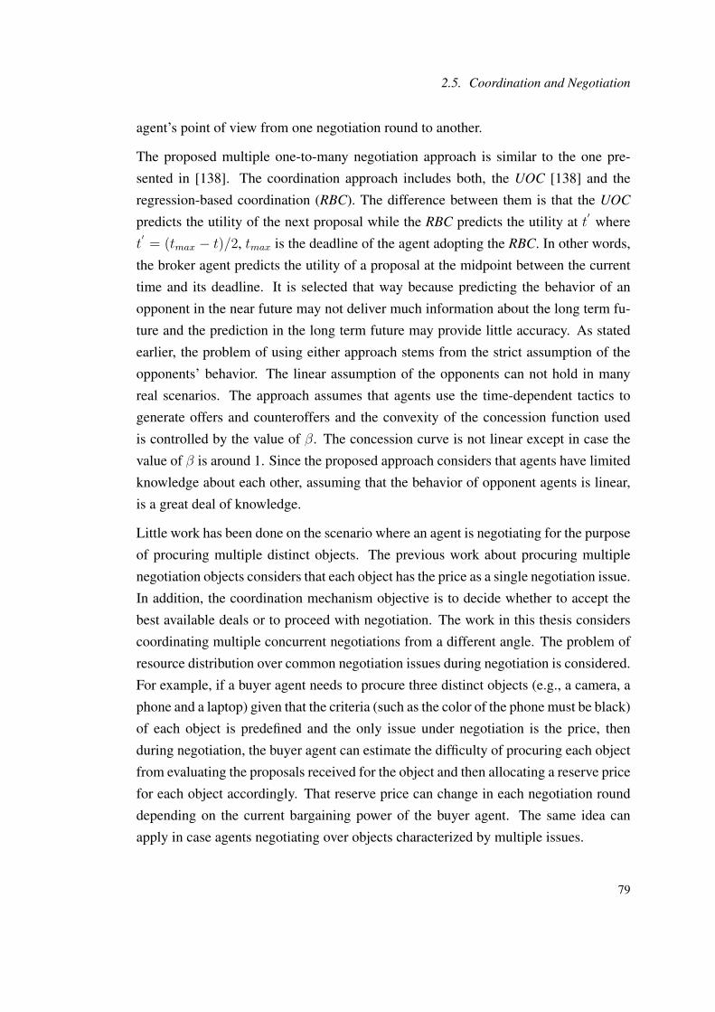
2.5. Coordination and Negotiation
agent’s point of view from one negotiation round to another.
The proposed multiple one-to-many negotiation approach is similar to the one pre-
sented in [138]. The coordination approach includes both, the UOC [138] and the
regression-based coordination (RBC). The difference between them is that the UOC
predicts the utility of the next proposal while the RBC predicts the utility at t′ where
t′
= (tmax − t)/2, tmax is the deadline of the agent adopting the RBC. In other words,
the broker agent predicts the utility of a proposal at the midpoint between the current
time and its deadline. It is selected that way because predicting the behavior of an
opponent in the near future may not deliver much information about the long term fu-
ture and the prediction in the long term future may provide little accuracy. As stated
earlier, the problem of using either approach stems from the strict assumption of the
opponents’ behavior. The linear assumption of the opponents can not hold in many
real scenarios. The approach assumes that agents use the time-dependent tactics to
generate offers and counteroffers and the convexity of the concession function used
is controlled by the value of β. The concession curve is not linear except in case the
value of β is around 1. Since the proposed approach considers that agents have limited
knowledge about each other, assuming that the behavior of opponent agents is linear,
is a great deal of knowledge.
Little work has been done on the scenario where an agent is negotiating for the purpose
of procuring multiple distinct objects. The previous work about procuring multiple
negotiation objects considers that each object has the price as a single negotiation issue.
In addition, the coordination mechanism objective is to decide whether to accept the
best available deals or to proceed with negotiation. The work in this thesis considers
coordinating multiple concurrent negotiations from a different angle. The problem of
resource distribution over common negotiation issues during negotiation is considered.
For example, if a buyer agent needs to procure three distinct objects (e.g., a camera, a
phone and a laptop) given that the criteria (such as the color of the phone must be black)
of each object is predefined and the only issue under negotiation is the price, then
during negotiation, the buyer agent can estimate the difficulty of procuring each object
from evaluating the proposals received for the object and then allocating a reserve price
for each object accordingly. That reserve price can change in each negotiation round
depending on the current bargaining power of the buyer agent. The same idea can
apply in case agents negotiating over objects characterized by multiple issues.
79

Chapter 2. Background and Related Work
The works in [89] [91] [88] investigate the scenario where a buyer agent seeks agree-
ments over multiple objects given that each object has several issues and a single
provider. The proposed approaches in [89] [91] depend on allocating the available
resources to the common issues of different objects dynamically during negotiation.
The works presented in [89] [91] investigate the process of adapting the local reserva-
tion (see Section 4.3) values during negotiation according to the behaviors of the ex-
isting opponents over the common issues. Each common issue is assigned (possibly) a
new local reservation value in every negotiation round. The work in [88] involves the
adaptation of both, the initially generated counteroffers and the issues’ counteroffers
weight matrix during negotiation. Instead of adapting the local reservation values, the
approach presented in [88] adapts a matrix that determines how much each delegate
should propose for each issue of each object at the start of every negotiation round.
In addition, Chapter 7 investigates a more complex negotiation scenario where the ob-
jective of the buyer agent is to procure multiple distinct objects where each object is
characterized by multiple issues and have multiple providers.
2.6 Summary
This chapter first introduces the multiagent systems and their potential application do-
mains including automated negotiation. The automated negotiation is introduced in
Section 2.2. The section highlights the importance of negotiation as a conflict reso-
lution mechanism and the most important research areas that are related to automated
negotiation. In addition, it discusses the pros and cons of adopting the concurrent
negotiation approach. Moreover, the potential application domains of automated ne-
gotiation are presented.
Section 2.3 introduces the main approaches to negotiation including the game-theoretic
approaches, the learning and reasoning approaches and the argument-based ones. In
addition, the heuristic-based approaches including the time-dependent, the behavior-
dependent and the mixed tactics are discussed. The advantages and disadvantages of
each of the mentioned approaches are discussed in terms of their practical application
and feasibility including their computational power and processing time needs. The
game-theoretic approaches have their limitations in their hard assumptions about the
kind of knowledge they require and the unbounded rationality of agents. The learning
80
2.6. Summary
and reasoning approaches require historical data and/or large amounts of computa-
tional and time resources. The argument-based mechanisms have a future potential
in facilitating negotiating complex matters but is still in its early stages. The heuris-
tic negotiation approaches are simple and more practical than the other approaches,
especially in the research oriented studies.
The dependencies and coordination where the sources of dependencies in the context
of negotiation are discussed in Section 2.4. This part defines the possible interdepen-
dencies amongst the objects of negotiation such as the objects’ procuring order and the
possible interdependencies amongst the issues of negotiation such as when a group of
issues share a resource such as money.
The last section is the coordination and negotiation section. It presents a short intro-
duction to the coordination mechanisms that are used in multiagent systems and shows
how negotiation is considered as one of these mechanisms. It also emphasizes that
the aim of this thesis is to coordinate the concurrent multi-bilateral negotiations. In
addition, the relevant related works on the one-to-many negotiation focusing on the
different coordination mechanisms proposed in the literature are presented.
Most of the one-to-many negotiations in the literature investigate the situation where
an agent seeks to procure a single object characterized by a single issue. Managing the
convexity of the concession curves and/or updating the reservation values during nego-
tiation are amongst the coordination techniques that are adopted in the related work as
well as in this thesis. When the negotiation scenarios involve a single object of a single
negotiation issue, novel coordination mechanisms that are based on managing the con-
vexity of the concession curves are proposed and benchmarked against the proposed
mechanisms in the literature.
In the related work, previous negotiation data (e.g., utility rates) or some knowledge
about the probability distribution of some key data (e.g., the reservation values of the
opponents) are used to coordinate different negotiations. The negotiation mechanisms
proposed for a buyer agent in this thesis use only the negotiation information in the
current negotiation, i.e., the values of the received offers in the current negotiation en-
counter. On the other hand, the case where agents negotiate multiple objects are rarely
addressed in the negotiation literature. The works presented here address the negotia-
tion scenarios where a buyer agent negotiates with multiple seller agents over multiple
objects, e.g., services. Other related works propose the decommitment management
81

Chapter 2. Background and Related Work
approach as a coordination mechanism where an agent is allowed to renege from a
previous agreement(s) by paying a penalty. The decommitment management approach
is not investigated in this thesis since the types of agreements considered are either
binding for the agents or such that the buyer agent has the privilege of reneging from
an agreement without paying penalty.
82
Chapter 3
General Negotiation Model
This chapter presents a novel negotiation model that captures various negotiation sce-
narios. The model emphasizes that the negotiation object is one of the main com-
ponents that are necessary for describing any negotiation scenario. The model de-
fines negotiation thread, negotiation instance, connected agreement and disconnected
agreement. It also introduces the term delegate for describing an agent’s component
that can negotiate with other agents on the behalf of the agent. In this case, the agent
can create and destroy any number of delegates during negotiation as needed. The
utility functions that are used to evaluate offers are also presented. Finally, since an
object can have one or more negotiation issues, an agent needs to decide when to
accept an offer, the offers’ evaluation decisions are discussed.
3.1 Introduction
The negotiation model is an important tool for describing any negotiation scenario. A
negotiation scenario in multiagent systems contains agents as the interacting compo-
nents. Agents need to have common interests over a certain object(s) which serve as
the purpose of interaction between them. In addition, agents need to know the things
that they need to negotiate which are represented as negotiation issues. Each negotia-
tion issue has constraints in which the agent cannot go beyond during negotiation. In
addition, agents need to follow a certain interaction rule. Moreover, the agents need to
be aware about the policy of accepting an agreement in different circumstances.

Chapter 3. General Negotiation Model
3.2 Overview of the Negotiation Model
The first part of this section presents the negotiation model in terms of its main compo-
nents: agents, negotiation objects and negotiation issues. In addition, it presents how
these components interrelate and the main assumptions of this of thesis. The second
part discusses how agents evaluate offers and counteroffers especially when negotiat-
ing multiple issues.
3.2.1 Negotiation Model
The following formalized negotiation model is general and can be used to describe var-
ious negotiation scenarios. The negotiation is presented by the tupleN =< O,S,D,J >
where,
1. O is the set of negotiation objects where agents have interest to negotiate over. A
negotiation object represents either a physical item (e.g., a printed book, a cam-
era etc.) or a non-physical item, e.g., a service, a resource etc. The set of objects
O = o1, ..., om, where oi stands for a negotiation object. It is assumed that
the O set contains all the negotiation objects and remains unchanged throughout
negotiation.
2. S is the set of seller agents in the current negotiation encounter, S = s1, ..., sm.If one or more negotiation objects have more than one provider, then si =
si1, ..., sini where i is the object identity in which the group si is aiming to
sell and ni is the number of seller agents that are willing to sell object oi, see
Figure 3.1, otherwise, si stands for a seller agent who is willing to sell the object
oi, see Figure 3.2.
3. D is the set of buyer agent’s negotiation delegates, D = d1, ..., dm. If one or
more negotiation objects have more than one provider, then di represents a set of
delegates, di = di1, ..., dini, that are responsible for buying object oi where i
is the object identity, ni is the number of the buyer agent’s delegates responsible
for buying object oi, see Figure 3.1. If object oi has one provider, then di stands
for a buyer’s delegate who is responsible for buying object oi, see Figure 3.2.
84
3.2. Overview of the Negotiation Model
4. J is the set of negotiation issues or attributes, J = j1, ..., jg, where ji is an
issue characterizing at least one negotiation object.
Figure 3.1: Complex one-to-many negotiation
In addition to the notation described above, the following assumptions are considered
in this thesis:
• |D| = |S|. It means the number of delegates are equal to the number of seller
agents at any point of time during negotiation. The delegates are created and
destroyed during negotiation to match the number of seller agents.
• ∀si ∈ S and ∀di ∈ D, |di| = |si|. It is similar to the previous point and applies
in case an object has multiple providers.
• ∀oi ∈ O, oi ∼ Jq where Jq ∈ 2J. It means that each object is characterized by a
set of issues. It is possible that two or more objects have the same set of issues.
• agents use the alternating offers protocol [125].
• in case of multi-issue negotiation, when an agent reaches an agreement over a
negotiation object, it means that the agent have an agreement over each issue
of that object using the object response and the issue response decision making
mechanisms, see Section 3.2.2
• each negotiating agent has a deadline by which the agent accepts an offer or
withdraws from negotiation.
• agents negotiate under incomplete knowledge, since the reservations values,
deadlines, utility structure and the offer generation models are private informa-
tion.
85
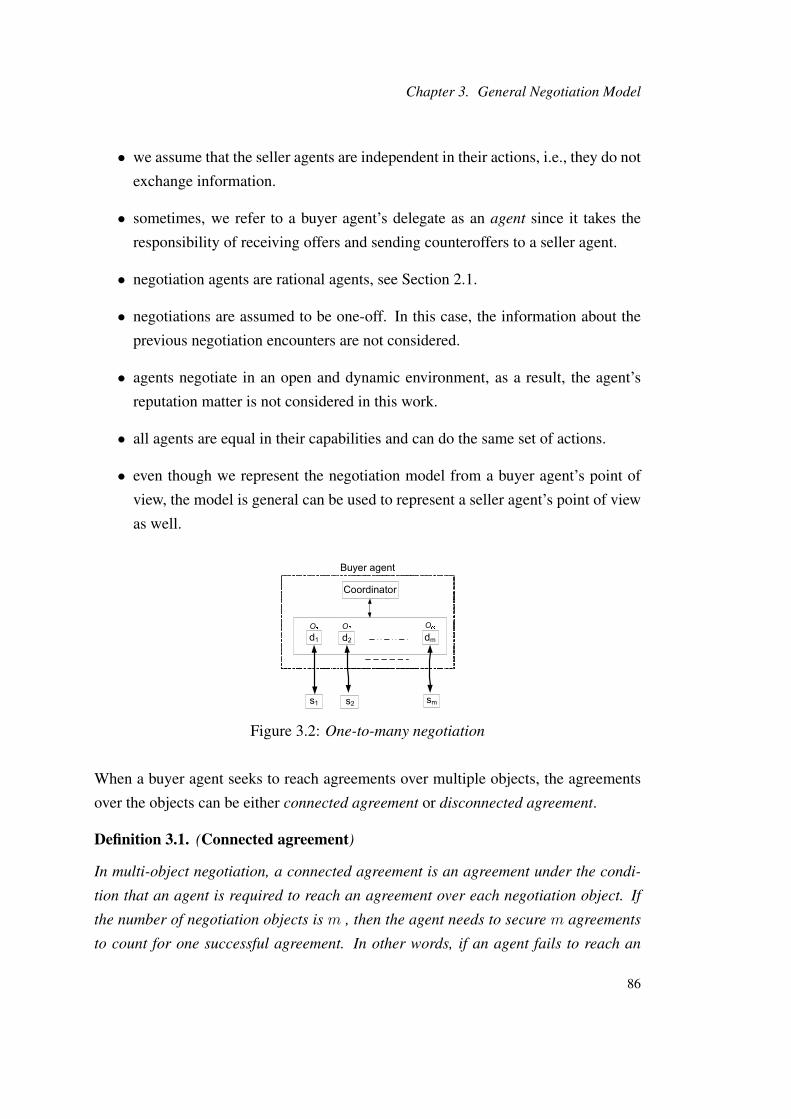
Chapter 3. General Negotiation Model
• we assume that the seller agents are independent in their actions, i.e., they do not
exchange information.
• sometimes, we refer to a buyer agent’s delegate as an agent since it takes the
responsibility of receiving offers and sending counteroffers to a seller agent.
• negotiation agents are rational agents, see Section 2.1.
• negotiations are assumed to be one-off. In this case, the information about the
previous negotiation encounters are not considered.
• agents negotiate in an open and dynamic environment, as a result, the agent’s
reputation matter is not considered in this work.
• all agents are equal in their capabilities and can do the same set of actions.
• even though we represent the negotiation model from a buyer agent’s point of
view, the model is general can be used to represent a seller agent’s point of view
as well.
Figure 3.2: One-to-many negotiation
When a buyer agent seeks to reach agreements over multiple objects, the agreements
over the objects can be either connected agreement or disconnected agreement.
Definition 3.1. (Connected agreement)
In multi-object negotiation, a connected agreement is an agreement under the condi-
tion that an agent is required to reach an agreement over each negotiation object. If
the number of negotiation objects is m , then the agent needs to secure m agreements
to count for one successful agreement. In other words, if an agent fails to reach an
86

3.2. Overview of the Negotiation Model
agreement over any negotiation object then the negotiation ends with a conflict deal
and the utility for that agent is assumed to be zero.
Similarly, an object agreement is considered a connected issue agreement since an
agent must reach an agreement over every issue.
Definition 3.2. (Disconnected agreement)
In multi-object negotiation, if an agreement over each negotiation object is not a strict
obligation, then an agreement over any object is considered a disconnected agreement.
One disconnected agreement counts for one agreement. An agent counts how many
disconnected agreements are achieved in a negotiation encounter for the purposes of
evaluating the negotiation process.
In case the agreements are of a disconnected type, an agent seeks to reach the largest
possible number of agreements and the overall utility of the final agreement is calcu-
lated by considering only the utilities of the objects in which the agent reaches agree-
ments over.
We assume that each negotiation delegate is responsible to negotiate over one object at
a given negotiation encounter (see function fd in Equation 3.1), while many delegates
may negotiate with many seller agents over the same object concurrently.
The negotiation scenario described in Figure 3.1 is a bit complicated since the coordi-
nator unit in the buyer agent needs to consider two levels of coordination, one at the
level of each object (i.e., local level) and another at the level of all objects, i.e., global
level.
In our model, each negotiation delegate is mapped to an object, a deadline tmax ∈ N∗,an offer generation strategy θ ∈ Θ, and an object weightWi ∈ (0, 1], see fd in Equation
3.1. The objects’ weights are used to calculate the weighted average utility of procuring
m objects under the assumption that the objects are independent andm∑i=1
Wi = 1.
fd : D1−1−−→ (O× N∗ ×Θ×Wi × ...)
fo : O1−1−−→ 2J
fj : J1−1−−→ ([min,max]× ...)
(3.1)
87
Chapter 3. General Negotiation Model
Each object is mapped to a negotiation issue set Jq where Jq ∈ 2J, see fo in Equation
3.1. Finally, each issue is mapped to a set of constraints, e.g., the interval of acceptance
([min,max]), where min,max represent either the starting offer value or the reserva-
tion value of a negotiation issue, see fj in Equation 3.1. When min is the starting offer
value then max is the reservation offer value and vice versa. Usually, a seller agent
starts proposing a high price (i.e., its max) for a certain item, then it may concede up
to its minimal acceptable price for this item, i.e., its min. The buyer agent behaves the
opposite way regarding the price issue.
In each negotiation round, the buyer agent may need to execute one or more of the
three functions (i.e., fd, fo, fj in Equation 3.1) as a response to some changes in the
negotiation environment, such as destroying a delegate as a result of withdrawing its
partner seller agent from negotiation or reaching an agreement over the object assigned
to that delegate, changing or updating the current negotiation tactic etc. The buyer
agent creates and destroys delegate negotiators during negotiation to match the number
of the existing seller agents.
We use the notation xtd→s
[Jq] to stand for the vector of values proposed by an agent d
to an agent s (s ∈ si, sil and d ∈ di, dil) at time t given that the xtd→s
[Jq] has a
value for each issue jl ∈ Jq and ∃ oi ∼ Jq. All the formulae included in this chapter
can be used by both agent types, i.e., d and s. To refer to a value of a certain issue
say [jl] ∈ xtd→s[Jq], we use the notation xt
d→s[jl]. Assume that agents are negotiating
over independent issues, let Ub(xts→d
[Jq]) be a function that computes the weighted
average utility of the agent d from receiving the offer xts→d
[Jq] at time t. The weighted
average utility of delegate d is computed according to Equation 3.2.
Ud(xts→d
[Jq]) =
|Jq |∑l=1
Wl ∗ ud(xts→d
[jl]), (3.2)
where|Jq |∑l=1
Wl = 1 and ud(xts→d
[jl]) is a function that calculates the utility gain of the
agent d from receiving the offer (xts→d
[jl]), see Equation 3.3 below. For m objects,
the agent computes m utility values. The total utility is calculated as the average of m
utility values given that all objects have the same importance (i.e., the same weight) to
the buyer agent. In case objects differ in their importance, the total utility is calculated
88

3.2. Overview of the Negotiation Model
as a weighted average of m utility values given that the objects under negotiation are
independent.
An agent uses equation 3.3 to compute the utility of a single issue offer. For example,
a buyer’s delegate d uses the utility function ud to evaluate an offer received from an
agent s over an issue jl:
ud(xs→d[jl]) =
(xs→d[jl]−RV djl
)/(IV djl−RV d
jl), If(IV d
jl> RV d
jl)
(RV djl− xs→d[jl])/(RV
djl− IV d
jl), If(IV d
jl< RV d
jl)
(3.3)
The buyer agent uses Equation 3.3 to evaluate both, the received offer over an issue
and its generated counteroffer over that issue. Similarly, with simple modifications,
Equations 3.2 and 3.3 can be used by the seller agents for the purpose of calculat-
ing the weighted average utility and the single issue offer utility, respectively, for the
counteroffers they receive and the offers they generate.
The set of offers and counteroffers that are exchanged between any negotiation pair
during the current negotiation encounter is called a negotiation thread. Formally, the
negotiation thread denoted by X td↔s
[Jq] is defined as follows:
Definition 3.3. (Negotiation thread)
Assuming that a seller agent s starts proposing at time t = 0, the negotiation thread
for the negotiation pair (d, s) over an object oi ∼ Jq at time t is denoted by X td↔s
[Jq],
where X td↔s
[Jq] =< xtd→s
[Jq], xt−1s→d
[Jq], xt−2d→s
[Jq], ..., x0s→d
[Jq] > . The first element
is optionally ∈ accept,withdraw. A negotiation thread X td↔s
[Jq] is active at time t
if first(X ts↔d
[Jq]) /∈ accept, withdraw where first(.) is a function that returns the
first element in a sequence.
The above definition is adapted from [33]. In general, the negotiation thread is consid-
ered the real-time information that is available for a negotiating agent. It can be used
in the process of decision making regarding the required action(s) in the next negoti-
ation round, e.g., withdraw from negotiation, what the value of the next offer is etc.
The decision making mechanisms proposed in this thesis rely on the active negotiation
threads as the source of real-time information. The negotiation threads can be used
to analyze the different patterns of concessions offered by different opponents in the
one-to-many negotiation.
89

Chapter 3. General Negotiation Model
To refer to a negotiation interaction between a buyer’s delegate and a seller agent, the
term negotiation instance is used.
Definition 3.4. (Negotiation instance)
A negotiation instance describes an active negotiation interaction between two agents.
The number of negotiation instances at a given time is equal to the number of active
negotiation pairs.
A negotiation instance is similar to a negotiation encounter. The difference is that
the negotiation instance describes an active negotiation encounter. In the one-to-many
negotiation, a negotiation instance is used to describe a negotiation encounter between
a buyer’s delegate and a seller agent. When the buyer agent creates a new delegate,
it actually creates a new instance which is a term borrowed from the object oriented
paradigm. Moreover, the negotiation encounter term is connected more to bilateral
negotiation.
The number of negotiation instances is dynamic in the one-to-many negotiation. For
example, when an agreement is reached between a delegate and a seller agent, the
number of negotiation instances is reduced by one and if a new seller agent engages in
negotiation, the number of negotiation instances is increased by one etc. In the one-to-
many negotiation, the number of active negotiation threads is equal to the number of
negotiation instances at any given time during negotiation.
3.2.2 Evaluation Decisions
When a buyer agent’s delegate d receives an offer for an issue jl from its opponent
seller agent s, it needs to evaluate the received offer using its utility function. If the
utility function does not exist, other evaluation criteria can be used such as existing
of minimum constraints accepting criteria or using certain ranking ordering rule. The
minimum constraints means that the agent accepts any offer that matches or exceeds
its minimal constraints. On the other hand, the rank ordering rule works when an agent
is able to rank its preferences over the decision variables and if the received offer is
aligned with this ranking, the offer is accepted. In this thesis, a utility function is used
in the evaluation process. In case of existing multiple negotiation issues and/or mul-
tiple negotiation objects, the negotiation decision mechanism needs to accommodate
90
3.2. Overview of the Negotiation Model
for the existing multiple decision variables. In case an object has multiple issues and
issues are different in their importance, the utility of the object’s offer is calculated as
a weighted average utility. Similar procedure is applied in case of existing multiple
objects. The difference is that the objects can also have different weights if they differ
in their importance from an agent’s point of view. When the negotiation objects have
different weights, the utility of each object is calculated as a weighted average utility
and the utilities of all objects are calculated again as a weighted average utility using
the objects’ weights instead of issues’ weights. The following definitions formalize the
evaluation decisions in different situations.
Definition 3.5. (Issue response I(.))
At the start of each negotiation round, an agent d takes an issue response I(.) decision
at time t′
regarding the received offer (xts→d
[jl]) given that t < t′
as follows:
Id(t′, xts→d[jl]) =
accept if(ud(xt
s→d[jl]) ≥ ud(xt
′
d→s[jl]) &(t
′ ≤ tdmax))
withdraw if(t′> tdmax)
send(xd→s[jl]) otherwise
(3.4)
The issue response (Id) considers the utility of the received offer by delegate d for an
object oi represented by the issue jl. The issue response in Equation 3.4 applies in case
agents are negotiating over a single issue. To handle the situation of multiple-issue
negotiation, Equation 3.5 is applied to each element of the composite offer to make
sure that the utility of each issue is not less than the utility of the reservation value of
that issue. Equation 3.5 is applied after the conditional accept decision is selected in
the object response, see Equation 3.6.
Id(t′, xt
s→d[jl]) =
accept if(ud(xt
s→d[jl]) ≥ ud(RV d
jl))
reject if(ud(xts→d
[jl]) < ud(RV d
jl))
withdraw if(t′> tdmax)
(3.5)
The modification of the offer acceptance condition in Equation 3.5 is connected to
the object response Bd(.) since the object response is concerned with the weighted
average utility of the received composite offer. Equation 3.5 does not have the send(.)
91

Chapter 3. General Negotiation Model
option since it is used only to check whether the utility of each issue’s offer of the
received composite offer that has the status conditional accept does not go beyond the
reservation utility of that issue, i.e., the minimum acceptable utility.
The accept and reject in Equation 3.5 are two labels that can be used to mark the status
of each issue. If the utility of a certain issue member of a received composite offer is
equal to or above the reservation utility of that issue, then the status of that issue will
be “accept”, otherwise, the status is “reject”.
Definition 3.6. (Object response B(.))
At the start of each negotiation round, an agent d takes an object response B(.) deci-
sion at time t′
regarding the received offer (xts→d
[Jq]) given that t < t′
as follows:
Bd(t′, xt
s→d[Jq]) =
conditional accept if(Ud(xt
s→d[Jq]) ≥ Ud(xt
′
d→s[Jq]) &(t
′ ≤ tdmax))
withdraw if(t′> tdmax)
send(xd→s) otherwise
(3.6)
The object response (Bd) considers the weighted average utility of the received offer
by delegate d for an object oi represented by the set of issues Jq.
If an agent d decides to conditionally accept an offer according to Bd, then it needs to
apply the issue response (Id) criteria shown in Equation 3.5 on each issue to make sure
that no issue receives a lower utility than its reservation utility. Because it is possible
that the weighted average utility of a certain composite offer is acceptable due to the
utility of a member offer (or more) is high whereas the utility of other member(s) of the
composite offer is/are under its/their reservation utility. In other words, the decision of
accepting a composite offer includes two steps, first, check the weighted average utility
of the received composite offer for a certain object and then check the individual utility
of each member of that offer. If the first result is true and the second result is true for
each member of the composite offer then the offer is accepted. Figure 3.3 shows the
decision process of accepting a multi-issue offer.
The other way around of making decisions over whether to accept a certain composite
offer is also possible. The agent starts inspecting the utility of each member of the
received composite offer and if all utilities are acceptable, the weighted average utility
92
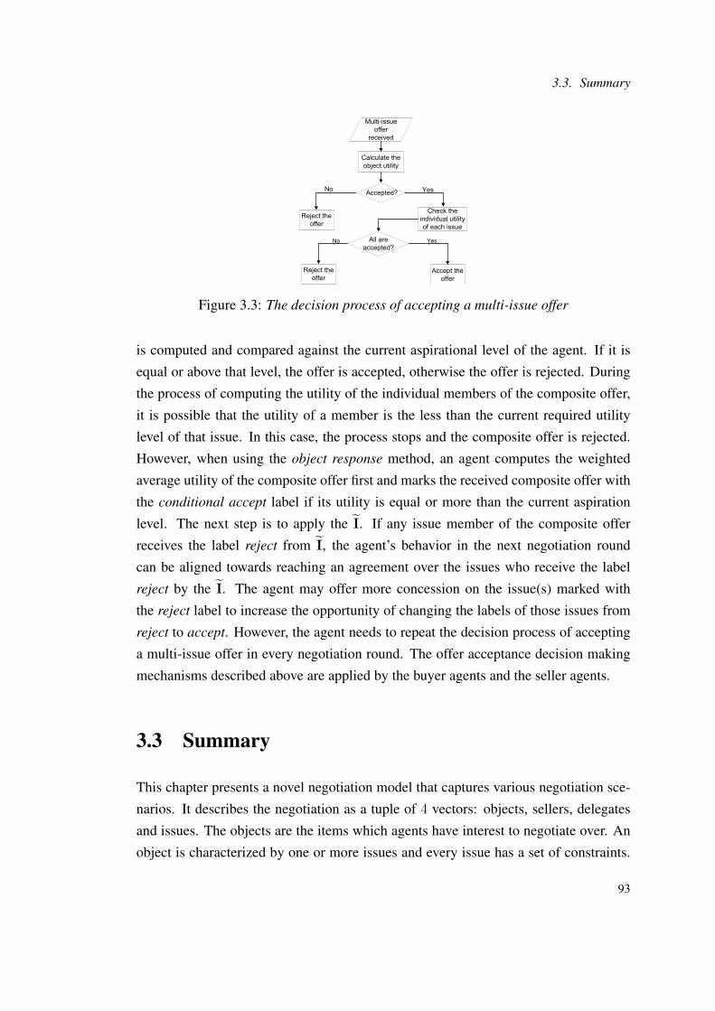
3.3. Summary
Figure 3.3: The decision process of accepting a multi-issue offer
is computed and compared against the current aspirational level of the agent. If it is
equal or above that level, the offer is accepted, otherwise the offer is rejected. During
the process of computing the utility of the individual members of the composite offer,
it is possible that the utility of a member is the less than the current required utility
level of that issue. In this case, the process stops and the composite offer is rejected.
However, when using the object response method, an agent computes the weighted
average utility of the composite offer first and marks the received composite offer with
the conditional accept label if its utility is equal or more than the current aspiration
level. The next step is to apply the I. If any issue member of the composite offer
receives the label reject from I, the agent’s behavior in the next negotiation round
can be aligned towards reaching an agreement over the issues who receive the label
reject by the I. The agent may offer more concession on the issue(s) marked with
the reject label to increase the opportunity of changing the labels of those issues from
reject to accept. However, the agent needs to repeat the decision process of accepting
a multi-issue offer in every negotiation round. The offer acceptance decision making
mechanisms described above are applied by the buyer agents and the seller agents.
3.3 Summary
This chapter presents a novel negotiation model that captures various negotiation sce-
narios. It describes the negotiation as a tuple of 4 vectors: objects, sellers, delegates
and issues. The objects are the items which agents have interest to negotiate over. An
object is characterized by one or more issues and every issue has a set of constraints.
93

Chapter 3. General Negotiation Model
Each delegate can negotiate with one seller agent over one object. In other words, a
delegate can be responsible for procuring only one object in any given interaction. The
proposed notation allows for the description of the situations where there is a single
provider per object and when an object can have multiple providers. The first case has a
single level of coordination, while the second case can have two levels of coordination.
The buyer agent creates a number of delegates equal to the number of seller agents that
are still in negotiation. If a seller agent quits negotiation or an agreement is reached
with a certain seller agent, its delegate partner is destroyed. Each delegate is assigned
an object and each object is assigned a set of issues. Finally, each issue is assigned a
set of constraints. The two main issue constraints that are used in this thesis are: the
issue reservation intervals and the issue weights vector.
The utility function that are used to evaluate offers and counteroffers are presented. The
utility function uses the minimum and the maximum values of the reservation interval
of a given issue to calculate the utility value for a received or generated offer for this
issue. The utility value can be any number in the closed interval [0, 1]. In addition, the
weighted average utility is explained. The agents use the alternating offers protocol
during their interaction.
The model also defines some relevant terms: negotiation thread, negotiation instance,
connected agreement and disconnected agreement. Finally, the model discusses the
evaluation decisions for the offers. Additional terms such as issue response and object
response mechanisms are proposed, defined and discussed. These mechanisms are
used in the offer accepting process.
94
Chapter 4
Coordination Scenarios and SolutionApproach
This chapter introduces the coordination problem in the concurrent multi-bilateral ne-
gotiation and emphasizes the coordination direction of this thesis. Possible negotiation
scenarios in multiagent systems are classified. The classification includes the bilateral
(i.e., one-to-one) negotiation and the multi-bilateral (i.e., one-to-many) negotiation
whereas the many-to-many negotiation can be formed by either. Five scenarios in the
one-to-many negotiation are identified and named coordination scenarios. Moreover,
the general solution approach is presented including a detailed example about the data
preparation. Finally, the general experimental settings are presented.
4.1 Coordination Problem in One-to-Many Negotiation
Consider a reverse auction where a buyer agent interacts with multiple seller agents.
Instead of adopting the reverse auction rules of encounter amongst agents, the alter-
nating offer protocol are assumed as a rule of the encounter. The buyer agent receives
multiple offers from the seller agents at time t and it responds at time t+ 1. In reality,
the responses of the seller agents may not be synchronized in terms of the time of their
response, however, for simplicity, all seller agents are assumed to send their offers at
the same time and the buyer sends its counteroffers to all seller agents at once. Each
agent has a deadline by which it either accepts an offer or withdraws from negotiation.

Chapter 4. Coordination Scenarios and Solution Approach
Unlike the reverse auction where the price is the only issue of interest for all agents,
we consider the situation where the agents are interested in negotiating over not only a
single issue, but over multiple issues such as delivery time, response, time etc.
When the buyer agent receives multiple offers at time t where t < tbuyermax , the buyer
agent can take one of two decisions: accept one or more of the received offers and quit
negotiation or reject some or all of the received offers and propose one or more coun-
teroffers. Some negotiation protocols allow the buyer agent to accept offers temporary
while in negotiation. As stated in Section 2.5.1, this thesis does not consider the prob-
lem of managing commitment/decommitment. The investigated cases are when the
buyer agent can renege on an agreement(s) without the need to pay penalty or it needs
to honor its agreement(s).
Certain mechanisms are proposed in the negotiation literature to coordinate the con-
current one-to-many negotiation. Most of the work focuses on tackling the following
two main coordination problems:
• the proposal accepting problem. Some coordination mechanisms (e.g., [138] [3]
[23]) are designed to answer the following question: when an agent receives a
number of offers in a certain negotiation round, should the agent accept the best
acceptable offer and quit negotiation? In this case the coordination mechanism
should consider different factors such as the value of the best existing offer, the
number of existing opponents, the agents’ deadlines and the expected utility of
the opponents’ future offers. The proposal accepting problem exists in all forms
of negotiation. Since deadlines and preference profiles are considered private
information of each agent, it becomes difficult for an agent to decide whether
to agree on an acceptable agreement or proceed with negotiation. If the buyer
agent accepts the best acceptable offer, it may lose a higher future offer value.
On the other hand, if the agent decides to continue in negotiation, it may not
reach an agreement at all since the deadlines of the opponent agents are private
information and the opponent agents may withdraw from negotiation at any time.
If an agent reaches its deadline during negotiation, i.e., current time t = tmax, the
dominant strategy for an agent is to accept the best acceptable offer. If t < tmax
then it becomes difficult to determine the dominant strategy. In case an agent
decides to proceed in negotiation, the risk of not reaching an agreement in case
of bilateral negotiation is higher than the case of multi-bilateral negotiation. In
96

4.1. Coordination Problem in One-to-Many Negotiation
multi-bilateral negotiation, an agent negotiates with multiple opponent agents
concurrently and the probability that all agents withdraw from negotiation at
once is less than the probability of a single agent withdrawing from negotiation.
• the bidding strategy problem. This problem tackles the problem of generating
offers (e.g., [118][18][40][34] [24]) for the next negotiation round. It can involve
defining either the offer value and/or the offer structure. Different methods are
proposed to generate offers such as using mathematical functions that depend on
the elapsed negotiation time and the value of the convexity parameter, imitation
offer generation mechanisms and mixing techniques, see Section 2.3.3. Other
methods are designed to propose trade-off offers to help reach an agreement
faster and at the same time do not jeopardize the utility of the proposer agent, see
Section 2.3.3.5. Even though manipulating the offer structure during negotiation
may help in reaching an agreement(s), its automation process is rarely addressed
in the negotiation literature.
The bidding strategy problem is an important problem in negotiation and in all nego-
tiation forms. It is a more challenging problem in the one-to-many negotiation since
the buyer agent needs to consider the behaviors of a number of opponents and a differ-
ent offer may need to be proposed to each opponent. Most of the work in this thesis
focuses on the bidding strategy in one-to-many negotiation. The focus is on devising
dynamic bidding strategies that consider the collective behaviors of the opponents in
terms of the their concession. The buyer agent uses only the received offers in the cur-
rent negotiation instance as source of data in the proposed dynamic bidding strategies.
The main coordination problem presented in this thesis is the problem of managing the
interdependencies between the generated counteroffers by a buyer agent negotiating
concurrently with a set of seller agents taking into consideration the behavior of each
seller agent. The interdependencies are managed by detecting the behaviors of the op-
ponent agents in terms of their concession behavior over different negotiation issues
in each negotiation round. The process is repeated in each negotiation round since the
seller agents may change their behaviors from one negotiation round to another.
97
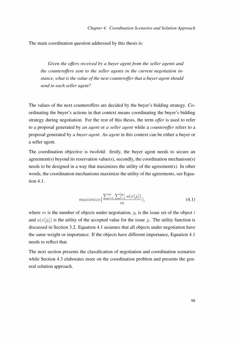
Chapter 4. Coordination Scenarios and Solution Approach
The main coordination question addressed by this thesis is:
Given the offers received by a buyer agent from the seller agents and
the counteroffers sent to the seller agents in the current negotiation in-
stance, what is the value of the next counteroffer that a buyer agent should
send to each seller agent?
The values of the next counteroffers are decided by the buyer’s bidding strategy. Co-
ordinating the buyer’s actions in that context means coordinating the buyer’s bidding
strategy during negotiation. For the rest of this thesis, the term offer is used to refer
to a proposal generated by an agent or a seller agent while a counteroffer refers to a
proposal generated by a buyer agent. An agent in this context can be either a buyer or
a seller agent.
The coordination objective is twofold: firstly, the buyer agent needs to secure an
agreement(s) beyond its reservation value(s), secondly, the coordination mechanism(s)
needs to be designed in a way that maximizes the utility of the agreement(s). In other
words, the coordination mechanisms maximize the utility of the agreements, see Equa-
tion 4.1.
maximize(∑m
i=1
∑|gi|l=1 u(x[jl])
m), (4.1)
where m is the number of objects under negotiation, gi is the issue set of the object i
and u(x[jl]) is the utility of the accepted value for the issue jl. The utility function is
discussed in Section 3.2. Equation 4.1 assumes that all objects under negotiation have
the same weight or importance. If the objects have different importance, Equation 4.1
needs to reflect that.
The next section presents the classification of negotiation and coordination scenarios
while Section 4.3 elaborates more on the coordination problem and presents the gen-
eral solution approach.
98

4.2. Coordination Scenarios
4.2 Coordination Scenarios
This section categorizes possible negotiation scenarios (adapted from the work pub-
lished in [86]) in multiagent systems taking into consideration the two main criteria
of a negotiation object that determine a particular negotiation scenario: the number
of negotiation issues and the number of opponents (providers) per object at a given
negotiation interaction. In addition, the number of the required agreements are added
to indicate the number of the required objects, see Figure 4.1. We consider that each
negotiation object requires one object agreement and each issue requires one issue
agreement. Formally, if an object oi has k issues, then we need k issue agreements to
make an object agreement over the object oi. For the rest of this manuscript, unless
stated to the contrary, an agreement means an agreement over an object.
Figure 4.1: Negotiation scenarios
Each of the three sub-nodes of the negotiation objects node shown in Figure 4.1 has
a cardinality of 1 or many. The Agreements node in Figure 4.1 refers to agreements
over objects given that each negotiation object requires one agreement. Saying that
an agent needs to reach N agreements is equivalent to saying that an agent needs to
secure N objects. When an agent seeks an agreement over multiple objects, it means
that the objects are distinct. For example, a camera and a TV are two distinct objects.
If the aim of a buyer is to negotiate with a seller agent for the purpose of buying two
identical objects (e.g., two cameras), then the model used in this work considers the
two identical cameras as one object taking into consideration the issues that can be
99

Chapter 4. Coordination Scenarios and Solution Approach
combined such as price and weight. When a buyer agent aims to buy several identical
objects, it can use this fact to strengthen its bargaining power. When many buyers
decides to make a coalition and submit one proposal to buy several objects at once,
that can help in strengthening the bargaining power of the buyer agents. However, the
agent coalition problem is not investigated here. For more information about agent
coalition, see [52] [76] [128].
As negotiation is one of the important interaction mechanisms in multi-agent systems,
considering the main criteria of negotiation objects (i.e., the number of issues per ob-
ject and the number of providers (opponents) per object) as shown in Figure 4.1, nine
negotiation scenarios are recognized. Amongst the nine negotiation scenarios, five are
identified and called coordination scenarios, namely, scenarios SSM, MSM, MMS,
SMM and MMM where the first letter stands for the number of negotiation objects
required, single or multiple, the second letter stands for the number of issues per nego-
tiation object, single or multiple and the third letter stands for the number of provider(s)
per object, single or multiple. For example, the SMM stands for the coordination sce-
nario where an agent seeks a single object characterized by multiple issues and there
are multiple providers for that object. These coordination scenarios are the study target
of this thesis. The coordination scenarios are investigated and a dynamic negotiation
strategy(s) is/are proposed for each. The proposed negotiation strategies control the
bidding process of a buyer agent negotiating concurrently with multiple seller agents
for the purpose of procuring one or more objects. All the coordination scenarios end
with the letter M except the scenario MMS. The scenario MMS targets the monopo-
listic markets where each object has a single provider.
As mentioned earlier, we assume that the number of objects is equal to the number of
agreements. Accordingly, we can decide whether an agent aims to procure one object
or more by looking at the arrow targeting the agreements node. If the arrow ends at 1
in Figure 4.1, then the number of objects is 1, otherwise the number of objects is more
than 1. The same logic applies for the issues and opponents nodes.
The first four scenarios shown with the dotted arrows in Figure 4.1 assume agents un-
dertake bilateral (i.e., one-to-one) negotiation where two agents engage in negotiation.
Scenario 1 in Figure 4.1 represents a situation where an agent is negotiating with one
opponent over one object characterized by a single issue. Negotiation scenario 2 refers
to a situation where an agent is negotiating with an opponent agent over multiple ob-
100

4.2. Coordination Scenarios
jects (N > 1) given that each object has a single issue. For example, a buyer agent
can negotiate with an electronic store agent over buying a TV and a camera of specific
criteria given that the only negotiation issue for each is the price issue. Negotiation
scenario 3 refers to a situation where an agent is negotiating with an opponent over
a single object characterized by several issues (L > 1). For example, an agent may
negotiate with a cloud storage provider over renting a storage space. The storage space
contains the issues: Price, storage size and duration of the storage.
Finally, scenario 4 describes a situation where an agent is negotiating with an oppo-
nent over multiple objects given that each object is characterized by several issues.
For example, a buyer agent can negotiate with an electronic store agent over buying
a camera and a TV given that each of them is characterized by several issues such as
price, warranty, delivery time, etc. This scenario is similar to scenario 7 (coordination
scenario MMS). The coordination scenario MMS assumes that each object has a dif-
ferent provider while scenario 4 assumes that all objects under negotiation have one
provider. The coordination approach proposed for scenario MMS may also apply for
negotiation scenario 4. However, in coordination scenario MMS, the variation in the
preference profiles of different agents are assumed to be more than the variation in the
preference profile assumed in negotiation scenario 4. For example, if all objects have
the same provider agent, then its preference over the price issue can be similar across
all objects while in case of scenario MMS, one provider may care about the price more
than about delivery time while other agents may have the opposite preference. Since
the proposed coordination mechanisms are based on the assumption of preference vari-
ations amongst the opponent agents, the coordination approach used in coordinating
the bidding strategy in scenario MMS is more effective than in scenario 4.
Since the work of this thesis focuses on coordinating the bidding strategy in one-to-
many negotiation, the bilateral negotiation is not investigated per se. However, some
of the offer generation methods used in bilateral negotiations are adopted in the one-
to-many setting.
The coordination scenario SSM represents an agent negotiating with multiple oppo-
nents over a single object characterized by a single issue. In real life, one may contact
several sellers before deciding to buy from any. For example, an agent can negotiate
concurrently with several opponents to buy a specific type of camera. This scenario
is investigated in Chapter 5. The difference between coordination scenarios SSM and
101

Chapter 4. Coordination Scenarios and Solution Approach
MSM is that an agent in scenario MSM is negotiating with multiple opponents for
the purpose of procuring several objects given that each object has multiple providers.
Each object in scenarios SSM and MSM has a single issue. As a real life example for
scenario MSM, a customer seeks to book both a flight and a room in a hotel by negoti-
ating with several carriers and several hotels. In this case, a customer agent negotiates
concurrently with several agents that can provide flight booking and several agents that
can provide hotel booking assuming that the customer agent seeks to secure the best
deals on the price of each, hence the price would be the only issue of negotiation for
both objects. Scenario MSM is investigated in Chapter 7.
Coordination scenario MMS refers to a situation where the purpose of an agent is to
secure multiple distinct objects (and hence multiple agreements are required) given
that each distinct object has one provider. This situation exists in monopoly markets
where there is only a single seller offering a certain product. When a buyer agent
needs to procure several distinct objects in a monopoly market, there would be a single
provider for each object.
The coordination scenario SMM represents an agent negotiating with several oppo-
nents for the purpose of securing an object characterized by several issues. This sit-
uation is abundant in real life. For example, an agent may find several carrier agents
to negotiate with over booking a flight. In this scenario, the customer agent cares, for
example, about the price, the date and the time of the flight that constitute the issues
of negotiation. This scenario is investigated in Chapter 6 where a meta-strategy is
proposed to coordinate the bidding strategy during negotiation.
Finally, the coordination scenario MMM considers a situation where an agent seeks
to secure several agreements over several objects given that each object has several
providers and several negotiation issues. This scenario is the most complex one. It
exists in markets where there are several providers for each distinct object and each
object contains multiple issues. For example, an agent can negotiate with several cloud
service provider agents (e.g., Amazon EC2, Google App Engine, AT&T Synaptic, etc.)
over a storage space and computations power in the cloud. The storage space can have
several issues such as price, size, duration, etc. The computational power can have
issues like price, response time etc. This scenario is investigated in Chapter 7.
102

4.3. Solution Approach
4.3 Solution Approach
When a buyer agent engages into multi-bilateral concurrent negotiation with a set of
seller agents, the buyer agent needs to coordinate its actions (see Section 4.1) against its
opponents in each negotiation round to achieve one or more of the negotiation objective
criteria such as utility gain and agreement rate.
Formally, let Ωa be the negotiation strategy of an agent a, then Ωa = 〈IV a, RV a, T a,Θa〉,where IV a, RV a, T a,Θa represent the vector of the initial offer/counteroffer values,
the vector of the reservation values, the deadlines vector and finally the vector of the
offer/counteroffer generation tactics of an agent a.
Our representation of an agent’s a strategy vector (i.e., Ωa) is similar to its repre-
sentation in [38]. The difference is that the fourth part of the strategy vector in [38]
represents the value β which is a parameter of functions normally used in the time-
dependent tactics, while the fourth part in our representation (i.e., Θa) is a more
general: it indicates any possible offer/counteroffer generation tactic, e.g., trade-off,
time-dependent, behavior-dependent etc., its associated parameters (e.g., β value) and
constraints. For example, if an offer generation tactic calculates a value beyond the
reservation value of an issue, then there should be a constraint to modify that value to
be the reservation value of that issue.
A change to any of the Ωa components during negotiation is considered a change in
agent a’s negotiation strategy. In this thesis, the negotiation strategy and the bidding
strategy are used interchangeably. In our work, we investigate how a bidding strategy
for each of the buyer agent delegates (a delegate is a component in the buyer agent
that interacts with one opponent agent, see Section 3.2) can be dynamically managed
or coordinated taking into consideration the behaviors of the active opponents during
negotiation. An active opponent is an opponent whose last offer is neither accept nor
withdraw, see Section 3.2. Based on the offers received from an active opponent, two
methods can be used to evaluate the opponent, the first one is called the difference
in concession measure (DIC) and the second one is called the last offer utility (LOU)
measure. The LOU uses the utility of the received last offers from all agents. When
the buyer agent uses DIC measure to evaluate the opponent agents, a data preparation
procedure is required.
To manage the bidding strategy during negotiation (in real-time) for a buyer agent ne-
103

Chapter 4. Coordination Scenarios and Solution Approach
gotiating concurrently with multiple seller agents assuming that the information about
each seller agent is the sequence of the offers received from each during the current
negotiation instance, the following steps are implemented:
1. select an appropriate strategy component(s) for manipulation. The selection of
a particular component for manipulation depends mainly on the coordination
scenario. For example, a trade-off negotiation mechanism is not an option in
coordination scenarios SSM and MSM since there is a single negotiation issue
and the negotiation game is of zero-sum type. Another factor is the type of the
counteroffer generation tactic the buyer agent chooses to use. For example, if the
buyer agent chooses to use the time-dependent tactics to generate counteroffers,
then the only parameters that can control the process of counteroffer generation
are the convexity and deadline parameters. In this case, these two parameters
are the only options that can be used to manage the bidding strategy during
negotiation.
2. the offers from each opponent is treated as a mathematical sequence and for
each sequence, the first order-difference (see [12]) sequence is constructed in
each negotiation round. Let X tsi→di
[jl] =< xt−1si→di
, xt−2si→di
, ..., xt=0si→di
> be the
sequence of offers sent from a seller agent si to a buyer’s delegate di over the
issue jl and let t be the current time, ∆si =< |xt−1si→di
− xt−2si→di
|, |xt−2si→di
−xt−3si→di
|, ..., |x1si→di
− xt=0si→di
| >, where ∆si is the first order difference of the
sequence X tsi→di
[jl]. The absolute sign is used to accommodate for two situa-
tions: the first case is when the initial offer value of a negotiation issue is larger
than the reservation value of that issue, such as the price issue for a seller agent.
The second case is when the initial value of an issue is smaller than the issue’s
reservation value, such as the quantity issue for a seller agent. The ∆si is cal-
culated for each seller in each negotiation round. Analogously, the ∆di is found
for each delegate di where the sequence is used to calculate ∆di is X tdi→si
[jl].
Depending on the mental state of the buyer agent, the concession behavior dur-
ing any part (partial sum or total sum) of the history of the offers received from a
seller agent si during the current negotiation instance can be used to evaluate the
behavior of the seller agent si. The sum of each ∆si is used if the buyer agent
considers the total concession of a seller agent since the start of negotiation. If
the buyer considers only the recent concession, it might consider the first element
104

4.3. Solution Approach
in ∆si, etc. If the buyer agent assume that the behaviors of the seller agents are
dynamic and non consistence, then it might consider the recent concession only.
3. during negotiation, the behavior of each seller agent is compared to the behavior
of its delegate counterpart. In other words, we do pairwise comparison between
the concession of a buyer’s delegate and its counterpart seller agent. The reason
is that different buyer’s delegates may behave differently during negotiation. For
example, if the vector of the first elements in each ∆si is <$3,$7,$2,$10,$4>
and the vector of the first elements in each ∆di is <$2,$5,$4,$12,$3>, then
the pairwise comparison involve finding the difference between the two vectors,
<$3,$7,$2,$10,$4> - <$2,$5,$4,$12,$3> = <$1,$2,$-2,$-2,$1>. It is obvious that
if we take the absolute amount of concession of each seller without doing the
pairwise comparison, the seller agent number 4 is offering the largest conces-
sion ($10). By doing the pairwise comparison we decide that the seller agent
number 4 is as good as the seller agent number 3, while the best seller agent
from the buyer agent point of view is the seller agent number 2.
4. the information obtained in points 2 and 3 are used to manipulate the compo-
nent(s) of point 1
5. counteroffers are generated according to the updated bidding strategy.
6. at the start of a new negotiation round, goto 1
Steps 2 and 3 above are the data preparation procedure necessary for the DIC measure.
The described steps are a general solution approach that can be used to manage the
bidding strategy of a buyer agent negotiating with multiple seller agents concurrently.
Similarly, the same approach can be adopted by a seller agent negotiating with multiple
buyer agents concurrently. The realization of the above steps are shown in the next
chapters.
The above approach is based on the following assumptions:
• agents are self-interested aiming at maximizing their utility gain per agreement
and willing to cooperate - if possible - to reach a win-win agreement
• agents keep their preferences and strategies private
105
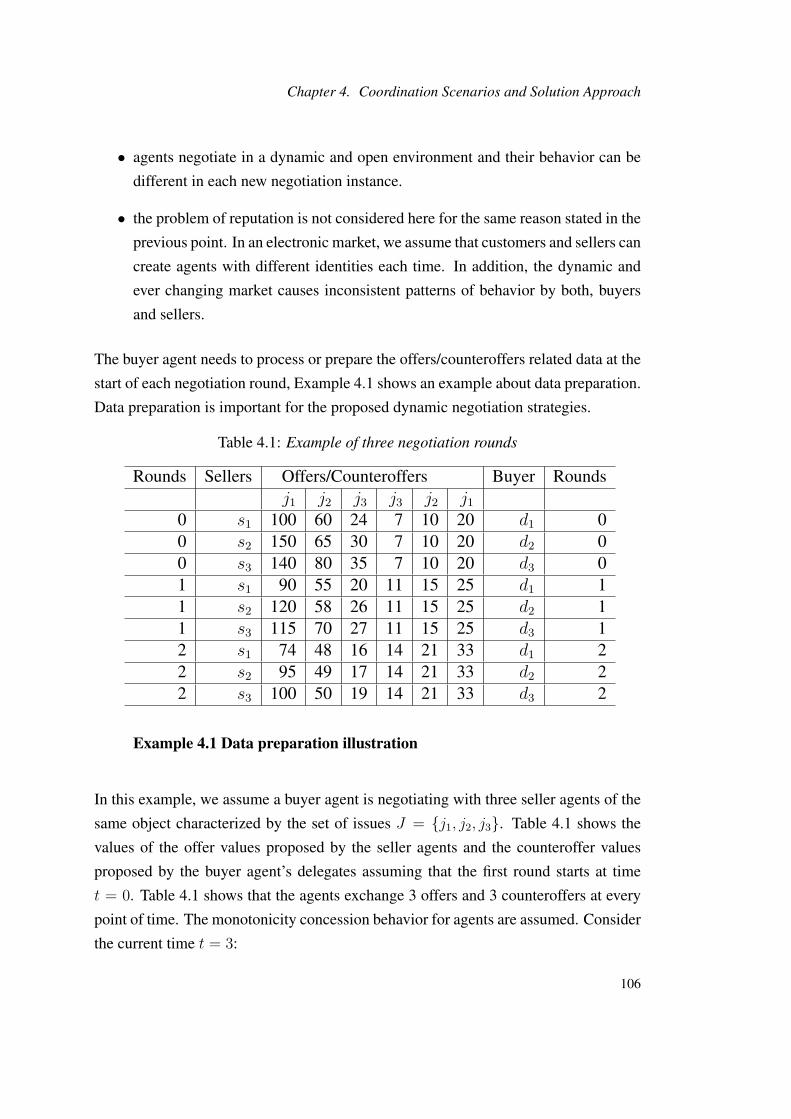
Chapter 4. Coordination Scenarios and Solution Approach
• agents negotiate in a dynamic and open environment and their behavior can be
different in each new negotiation instance.
• the problem of reputation is not considered here for the same reason stated in the
previous point. In an electronic market, we assume that customers and sellers can
create agents with different identities each time. In addition, the dynamic and
ever changing market causes inconsistent patterns of behavior by both, buyers
and sellers.
The buyer agent needs to process or prepare the offers/counteroffers related data at the
start of each negotiation round, Example 4.1 shows an example about data preparation.
Data preparation is important for the proposed dynamic negotiation strategies.
Table 4.1: Example of three negotiation rounds
Rounds Sellers Offers/Counteroffers Buyer Roundsj1 j2 j3 j3 j2 j1
0 s1 100 60 24 7 10 20 d1 00 s2 150 65 30 7 10 20 d2 00 s3 140 80 35 7 10 20 d3 01 s1 90 55 20 11 15 25 d1 11 s2 120 58 26 11 15 25 d2 11 s3 115 70 27 11 15 25 d3 12 s1 74 48 16 14 21 33 d1 22 s2 95 49 17 14 21 33 d2 22 s3 100 50 19 14 21 33 d3 2
Example 4.1 Data preparation illustration
In this example, we assume a buyer agent is negotiating with three seller agents of the
same object characterized by the set of issues J = j1, j2, j3. Table 4.1 shows the
values of the offer values proposed by the seller agents and the counteroffer values
proposed by the buyer agent’s delegates assuming that the first round starts at time
t = 0. Table 4.1 shows that the agents exchange 3 offers and 3 counteroffers at every
point of time. The monotonicity concession behavior for agents are assumed. Consider
the current time t = 3:
106
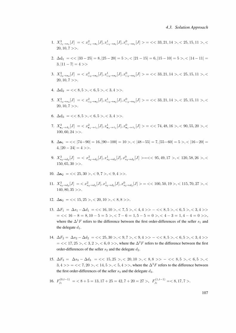
4.3. Solution Approach
1. X3d1→s1
[J ] = < x2d1→s1
[J ], x1d1→s1
[J ], x0d1→s1
[J ] > = << 33, 21, 14 >,< 25, 15, 11 >,<
20, 10, 7 >>.
2. ∆d1 = << |33− 25| = 8, |25− 20| = 5 >,< |21− 15| = 6, |15− 10| = 5 >,< |14− 11| =3, |11− 7| = 4 >>
3. X3d2→s2
[J ] = < x2d2→s2
[J ], x1d2→s2
[J ], x0d2→s2
[J ] > = << 33, 21, 14 >,< 25, 15, 11 >,<
20, 10, 7 >>.
4. ∆d2 = << 8, 5 >,< 6, 5 >,< 3, 4 >>.
5. X3d3→s3
[J ] = < x2d3→s3
[J ], x1d3→s3
[J ], x0d3→s3
[J ] > = << 33, 21, 14 >,< 25, 15, 11 >,<
20, 10, 7 >>.
6. ∆d3 = << 8, 5 >,< 6, 5 >,< 3, 4 >>.
7. X3s1→d1
[J ] = < x2s1→d1
[J ], x1s1→d1
[J ], x0s1→d1
[J ] > = << 74, 48, 16 >,< 90, 55, 20 >,<
100, 60, 24 >>.
8. ∆s1 =<< |74−90| = 16, |90−100| = 10 >,< |48−55| = 7, |55−60| = 5 >,< |16−20| =4, |20− 24| = 4 >>.
9. X3s2→d2 [J ] = < x2s2→d2 [J ], x1s2→d2 [J ], x0s2→d2 [J ] >=<< 95, 49, 17 >,< 120, 58, 26 >,<
150, 65, 30 >>.
10. ∆s2 = << 25, 30 >,< 9, 7 >,< 9, 4 >>.
11. X3s3→d3 [J ] = < x2s3→d3 [J ], x1s3→d3 [J ], x0s3→d3 [J ] > = << 100, 50, 19 >,< 115, 70, 27 >,<
140, 80, 35 >>.
12. ∆s3 = << 15, 25 >,< 20, 10 >,< 8, 8 >>.
13. ∆F1 = ∆s1−∆d1 =<< 16, 10 >,< 7, 5 >,< 4, 4 >> − << 8, 5 >,< 6, 5 >,< 3, 4 >>
= << 16 − 8 = 8, 10 − 5 = 5 >,< 7 − 6 = 1, 5 − 5 = 0 >,< 4 − 3 = 1, 4 − 4 = 0 >>,where the ∆1F refers to the difference between the first order-differences of the seller s1 andthe delegate d1.
14. ∆F2 = ∆s2 −∆d2 = << 25, 30 >,< 9, 7 >,< 9, 4 >> − << 8, 5 >,< 6, 5 >,< 3, 4 >>
= << 17, 25 >,< 3, 2 >,< 6, 0 >>, where the ∆2F refers to the difference between the firstorder-differences of the seller s2 and the delegate d2.
15. ∆F3 = ∆s3 − ∆d3 = << 15, 25 >,< 20, 10 >,< 8, 8 >> − << 8, 5 >,< 6, 5 >,<
3, 4 >> = << 7, 20 >,< 14, 5 >,< 5, 4 >>, where the ∆3F refers to the difference betweenthe first order-differences of the seller s3 and the delegate d3.
16. F (0,t−1)j1
= < 8 + 5 = 13, 17 + 25 = 42, 7 + 20 = 27 >, F(1,t−1)j1
=< 8, 17, 7 >.
107
Chapter 4. Coordination Scenarios and Solution Approach
17. F (0,t−1)j2
= < 1 + 0 = 1, 3 + 2 = 5, 14 + 5 = 19 >, F(1,t−1)j2
= < 1, 3, 14 >.
18. F (0,t−1)j3
= < 1 + 0 = 1, 6 + 0 = 6, 5 + 4 = 9 >, F(1,t−1)j3
= < 1, 6, 5 >.
19. F t−1,t =< F(t−1,t)j1
, F(t−1,t)j2
, ... >
The result of the pairwise comparison between the seller agents of issue jl and their
counterparts delegates are denoted by F (t1,t2)jl
. The t1 and t2 are the conceding time
interval (CTI). The CTI includes the start time and the end time in the current nego-
tiation thread where the concessions of agents are considered. For example, at time
t = 3, the F (0,t−1)j1
indicates that the buyer agent considers all the concessions from the
starting time of negotiation till time t = 2 whereas the F (1,t−1)j1
indicates that it consid-
ers the concessions from time t = 1 till time t = 2. The buyer agent decides the values
of t1 and t2 depending on its belief about the important time interval of opponents’
behaviors. If it believes that the recent concessions are the most important ones, then
the first elements (or the first few elements) in the ∆F are considered.
By inspecting our example, the F (0,t−1)j3
= < 1, 6, 9 > is the pairwise comparison of
the seller agents’ concessions on the first issue (j1). It shows that the agent number
3 is the most generous while agent number 1 is the least generous. When we con-
sider only the recent concessions, F (0,t−1)j3
= < 1, 6, 5 >, the agent number 2 is the
most generous agent. This example shows that choosing the location and the length
of the time interval ([t1, t2]) of the current negotiation instance can affect the process
of coordination in terms of distinguishing between the behaviors of different agents.
In our experiments, two situations are considered, the recent concessions and the total
concessions up to the current negotiation round.
Example 4.1 shows an illustration for data preparation when a buyer agent is negotiat-
ing with three same object sellers where the purpose is to secure one object. Similar
approach is used to process the current negotiation threads (see Section 3.2) for more
complex scenarios. Once the F (t1,t2)jl
is found for each issue, the proposed coordination
mechanisms utilizes the current information in controlling one or more of the strategy
components during negotiation. The difference in concession method is one possible
approach to evaluate the behavior of a seller agent. A second approach to evaluate
the behaviors of the seller agents is to compare the utility values of their last proposed
offers. More detail about the second approach is presented in Chapter 5.
108

4.4. Global and Local Reservation Values
Since seller agents are assumed to be competitive and self-interested during negotiat-
ing, the buyer agent plays tough with the conceding seller agents and behaves more
lenient with the tough negotiating agents. The reason is that, a conceding agent is
more desperate to reach an agreement than a tough negotiating agent. The buyer agent
seeks to reach a high utility agreement with a conceding agent and reach an agree-
ment with tough agents since the worst case for the buyer agent is not to reach an
agreement. However, the proposed negotiation strategies consider the welfare of other
agents when agents are negotiating over objects characterized by several issues given
that agents have divergent preferences over issues. The proposed iterative offer genera-
tion mechanism is designed to be competitive and cooperative. It is competitive in case
the proposing agent using a concession strategy and cooperative when the proposing
agent uses a trade-off strategy, see Chapter 6 for details.
4.4 Global and Local Reservation Values
As reservation values are part of an agent negotiation strategy and since Chapter 7 fo-
cuses on managing the local reservation values during negotiation, it is important to
differentiate between global and local reservation values. We assume that global reser-
vation values are fixed during negotiation while local reservation values are subject to
change during negotiation. For example, a buyer agent negotiates over 2 objects o1 and
o2 which are characterized by the price issue. The buyer’s budget, which is $100, is
the global reservation value. The global reservation value can be divided amongst the
two objects’ common issue, i.e., the price issue. Assume that the buyer agent valuates
the object o1 by $60 and the object o2 by $40. The values $60 and $40 can change
during negotiation but their sum will always be $100. Hence the $60 and $40 are the
local reservation values and the $100 is the global reservation value for the price issue.
The same idea is applied for other common issues.
The global and local reservation values are important concepts in negotiation. Almost
every one of us practices managing the local reservation values. For example, let us
say I need to buy a laptop and a phone and my budget is $1000. Before checking
the market, it would be difficult for me to say how much I would spend on each. I
probably could say that the laptop may cost around $600. It can happen that during the
shopping process, I find a sale on a certain laptop brand that brought their prices from
109
Chapter 4. Coordination Scenarios and Solution Approach
$1200 down to $750. In that case, I may allocate the $750 to buy the laptop and find
a phone with around $250. By doing that, I am managing the local reservation values
over my items according to the current information in the market.
In automated negotiation, if a certain resource can be divided amongst different objects
such as the price resource, then there would be local reservation values which can
be modified during negotiation to achieve the main goal of negotiation which is, for
example, buying a certain number of distinct objects given the global reservation value.
4.5 General Experimental Settings
The dynamic negotiation strategies (bidding strategies) proposed in this thesis are eval-
uated empirically since it is difficult to evaluate the proposed mechanisms theoretically
due to the dynamicity nature of the one-to-many negotiation process. In particular, the
proposed mechanisms are based on heuristics. Moreover, there are a number of in-
terrelated negotiation variables that can affect the outcome of the negotiation process
such as different negotiation tactics, their associated parameters and deadlines which
makes theoretical validation difficult. The proposed algorithms are tested against sets
of negotiation variables that are constructed from using different combinations of these
variables to represent a realistic situation. For each different combination of variables,
experiments are conducted and results are analyzed.
The objectives of the proposed coordinated negotiation models to be maximized are
both, the utility of an agreement and the total number of agreements. In addition, some
models are tested for possible social welfare gain. In short, the dependent variables in
the proposed models are utility rate, agreement rate and social welfare. On the other
hand, there are many independent variables such as deadlines, overlaps, tactics and
their parameters, etc. More detail about the specific independent variables considered
in the experiments are discussed in the chapters to come. The next two sections discuss
the simulation environment and the general experimental setup.
110

4.5. General Experimental Settings
4.5.1 Simulation Environment
The Mathematica 8.0 in the Wolfram Workbench 21 environment is the technology and
platform used for building and running the experiments. Figure 4.2 shows a snapshot
of the development environment. The proposed negotiation strategies are structured
according to the specific coordinated negotiation scenario. Accordingly, the experi-
mental works are grouped in different projects. Some functions are used across dif-
ferent projects such as the time-dependent and behavior-dependent offer generation
mechanisms.
Figure 4.2: A snapshot of the experimental working environment
An agent in the experiments is abstracted as a negotiation strategy that generates offers
and counteroffers. In addition, it determines when to accept an offer and when to
withdraw from negotiation.
1Wolfram Workbench: www.wolfram.com/products/workbench/
111

Chapter 4. Coordination Scenarios and Solution Approach
4.5.2 Experimental Settings
Heuristic-based offer generation methods are often used in the negotiation literature
to evaluate different negotiation strategies, e.g., [33][38] [4]. The heuristic methods
discussed in sections 2.3.3.1 and 2.3.3.3 are used to generate offers and counterof-
fers by different agents. As shown in Section 2.3.3.1, time-dependent tactics contain
three -broadly speaking- types of concession behaviors: Boulware, linear and con-
ceder. If we use a combination of them to generate an offer using weights indicating
the percentage of participation of each type in the offer, wide range of offer types can
be created. When the behavior-dependent tactics are mixed with the time dependent-
tactics, a wider range of offers can be generated that reflect different possible types of
agents. Accordingly, the mixing technique ensures that the results of the experiments
are more robust. As explained in Section 2.3.3.3, the behavior-dependent tactics are
reactive towards the opponent concessions since they imitate the concession of the op-
ponent. Mixing a resource dependent offer generation method such as time-dependent
with a reactive offer generation method such as behavior-dependent assures testing the
proposed dynamic negotiation strategies against large and different possible types of
opponents. Table 4.2 shows a sample of tactics and the their intervals of weights.
Polynomial decision function: Conceder: PC = β|β ∈ [2, 10](Time-dependent) Linear: PL = β|β ∈ [0.9, 1]
Boulware: PB = β|β ∈ [0.1, 0.8]Mixing of time-dependent tactics: MTD: PC ∗ r1 + PL ∗ r2 + PB ∗ r3,
∑3i=1 ri = 1
Behavior-dependent concession Tit-For-Tat:a ∈ [0, 0.5)A = 1− a
Weights Small: S = µ|µ ∈ [0.1, 0.3]Medium: M = µ|µ ∈ (0.3, 0.6]Large: L = µ|µ ∈ (0.6, 0.9]
Table 4.2: Negotiation tactics, their parameters and weights for possible mixing be-tween different tactics
In Figure 2.4, the polynomial and the exponential concession functions show some-
how different convexity at different β values. For example, the linear behavior of the
exponential function lies roughly between 2 and 4, i.e., β ∈ [2, 4] whereas the linear
behavior for the polynomial function happens when β = 1. Values of β that are near
112

4.5. General Experimental Settings
1 also show close to linear behavior for the polynomial function. The values in Table
4.2 reflect the behavior of the two functions. Since the Sigmoid function behaves dif-
ferently from the polynomial and the exponential, it is excluded from the experiments.
For the behavior-dependent tactic, the concession Tit-For-Tat tactic is chosen because
its flexibility, see Section 2.3.3.4.
The negotiation tactics shown in Table 4.2 and their parameters can be mixed to pro-
duce a range of different concession behaviors. The Cartesian product between the
different components in Table 4.2 can be applied to generate a set of hybrid tactics.
For example, a set containing the polynomial time-dependent tactics and the behavior-
dependent tactics using different weights to mix between them is shown in Equation
4.2.
ST = polynomial × concession T it− For − Tat × weights
ST = PC, PL, PB × a,A × S,M,L(4.2)
The following is the result of applying the Cartesian product in Equation 4.2:
ST = (PC × a× S), (PC × a×M), (PC × a× L), (PC ×A× S),
(PC ×A×M), (PC ×A× L), (PL× a× S), (PL× a×M),
(PL× a× L), (PL×A× S), (PL×A×M), (PL×A× L),
(PB × a× S), (PB × a×M), (PB × a× L), (PB × a× S),
(PB ×A×M), (PB ×A× L)
(4.3)
Since the polynomial and the exponential functions behave similarly, the polynomial
function is used to generate offers and counteroffers by agents when they use the time-
dependent tactics. In the context of mixed tactics used in this thesis, an abbrevia-
tion such as PCaS means the mixed tactic PCaS uses the polynomial function with
a conceder behavior mixed with the concession Tit-For-Tat behavior-dependent (see
Equation 2.11) tactic where the contribution of the concession Tit-For-Tat behavior-
dependent in the final offer is small, i.e., S = µ|µ ∈ [0.1, 0.3]. Finally, the a in
PCaS means that the contribution of the opponent’s previous concession is a small part
(a ∈ [0, 0.3], see Table 4.2) of the offer being proposed using the concession Tit-For-
Tat behavior-dependent tactic, see Equation 2.11, whereas A indicates the opposite,
see Table 4.2. The rest of the abbreviations can be interpreted analogously. In some
experiments, the random absolute Tit-For-Tat is used instead, see Equation 2.9.
113

Chapter 4. Coordination Scenarios and Solution Approach
Each member of the ST set (see Equation 4.3) represents a subset of related con-
cession behaviors (the β parameter within the conceder behavior can have different
values, see Table 4.2) to ensure that the proposed bidding strategies are tested against
a wide range of opponents’ behaviors. In other words, to improve the diversity of op-
ponent’s behaviors, there are distinct groups of behaviors and the members of each
distinct group shows some variation. Specific experimental settings are presented in
the experimental evaluation part of each chapter.
The Mixing of time-dependent tactics (MTD) is introduced to ensure more variety in
the behavior of the opponent agents. The set r′ = r′1, r′2, r
′3 is generated randomly
from the interval [0, 1], then it is divided by its total (r = r′/sum(r
′)) to make sure
that the total of r = r1, r2, r3 equals 1. The previously generated PC,PL,PB are
multiplied by the set r as shown in Table 4.2.
In the experimental part of this thesis, we consider that agents are mostly driven by
their internal resource(s) such as time. However, in some experiments, the seller
agents are designed to use tactics that mix between the behavior-dependent and the
time-dependent tactics given that the contribution of the behavior dependent-tactics in
the final offer values are small to medium. The reason is that the actions of agents
are subject to the availability of certain resources and if agents are imitating their op-
ponents and do not care about the availability of their resources, e.g., time, then they
will just imitate their opponents which seems irrational and naive. If two agents do
not have time limitation, then the dominant strategy for an agent is to offer the mini-
mum amount of concession imposed by the system. If the opponent agent imitates its
counterpart, it will propose similar amounts of concessions. Given the situation, it can
not be sure that the two agents can reach an agreement within a reasonable time frame
especially if the minimum amount of allowed concession is very small.
In addition to the behaviors of the opponents in terms of their negotiation strategies,
two other important negotiation environmental factors need to be taken into consider-
ation: The percentage of overlap and the deadlines. The percentage of overlap deter-
mines the length of the agreement zone between negotiators. The overlap percentage
between the reservation value intervals of negotiation issues is an important factor for
the result of the final outcome of the negotiation process. In case the percentage of
the overlap is zero, then reaching an agreement becomes impossible. For example,
assume that the reservation interval for the price issue of a buyer agent is [10, 20] and
114
4.5. General Experimental Settings
the reservation interval for the price issue of an opponent seller agent is [40, 21]. In
this case the buyer agent, ultimately, will offer its reservation price as the last option
which is 20 and the seller agent offers its reservation price as the last proposal which is
21. It is obvious that the two agents will not come to an agreement because the overlap
between their reservation intervals is zero. In other words, there is no agreement zone
between the two agents.
The ramification of having small overlap percentage(s) (i.e., small agreement zones)
and agents having different deadlines is that the chance for reaching an agreement be-
comes slight since a buyer agent may concede up to its reservation price at its deadline.
At the same time, the seller agents can have different deadlines which means it can be
difficult to guarantee that at least one seller agent has the same deadline as the buyer
agent. If a seller agent and the buyer agent has the same deadline, then both will offer
their reservation value at the same time an agreement is reached.
In some experiments, different percentages of overlaps are incorporated to test for the
effect of the length of the agreement zone length on the negotiation outcome. Sup-
pose that an agent d has the reservation interval [mindjl ,maxd
jl] for an issue jl, the
reservation interval of the issue jl of an opponent agent s is calculated as follows:
[minsjl ,maxs
jl] =
minsjl = mindjl + Φjl(maxdjl−mindjl)
maxsjl = minsjl + (maxdjl −mindjl
)(4.4)
In Equation 4.4, Φjl is the overlap percentage (Φjl ∈ [0, 1]) that determines the agree-
ment zone length between the two agents for the issue jl. For example, when Φjl = 0,
there is a complete overlap while if Φjl = 1 then the two agents meet exactly at their
reservation values and an agreement is only possible if both agents offer their reserva-
tion values. If Φjl = 0.4, then the percentage of the overlap is 60% etc. Using different
Φjl values result in different percentages of overlaps.
The deadline is an important factor in negotiation. In real negotiation environment, the
length of the negotiation time is finite and can be determined either by the negotiation
environment or by the individual agents. If the deadline is determined by the environ-
ment then all agents will have the same deadline, otherwise, each agent chooses its
own deadline according to its mental state. Deadlines are related to reservation values
in the sense that agents offer their reservation values at their deadlines. In addition,
115
Chapter 4. Coordination Scenarios and Solution Approach
a deadline is a parameter used in the time-dependent tactics to decide the value of an
offer for the next negotiation round.
The number of exchanged messages in terms of offers and counteroffers between
agents coined in the term negotiation rounds can be used instead of considering the
real negotiation time for testing different negotiation strategies which is a widely used
approach in the negotiation literature, e.g., [35][164][40]. In this thesis, the concept of
negotiation round is used and one negotiation round is equivalent to one time unit. A
negotiation round involves the exchange of two offers between two agents. If an agent
s starts a negotiation round by proposing an offer at time t = 0, then an opponent agent
d replies with a counteroffer at time = 1. This makes a complete negotiation round.
For example, if the deadline is assumed to be 20 then the number of negotiation rounds
is 20 and each agent proposes 20 offers and receives 20 counteroffers etc.
The results of the experiments are averaged and plotted. The error-bars are shown to
indicate the significance of the results. In addition, the Mann-Whitney test [85] is used
to ensure that the differences between the results are statistically significant at 95%
confidence level.
4.6 Summary
This chapter introduces the coordination problem in the one-to-many negotiation. An
agent (a buyer agent in our case) is assumed to conduct multi-bilateral negotiations
with a group of seller agents concurrently given that the buyer’s concurrent negotia-
tions have a common goal. Accordingly, the state of a certain instance of negotiation
can affect the state(s) of the other instances. In other words, the concurrent negotiations
can be interdependent. The interdependency between different negotiations causes the
need for coordination.
Section 4.2 in this chapter classifies possible negotiation scenarios and names the 5
one-to-many negotiations as coordination scenarios. The reason for choosing this
name is that the negotiation scenarios require coordination between the concurrent
negotiations of each type given the assumption that they aim to achieve a common
goal. The classification scheme is based on the numbers of the main components of
any negotiation: objects, issues and providers. The number of these components can
116

4.6. Summary
be either single or multiple. Since this thesis targets the one-to-many negotiation, the
number of the opponents per object is assumed to be multiple, except for the case when
the objective of the buyer agent is to procure multiple distinct objects in a monopolistic
market where each object has a single provider.
The solution approach for coordinating multiple negotiations is presented in Section
4.3. The proposed approach assumes that the only available information during nego-
tiation is about the offers received from the current seller agents. Since the buyer agent
is assumed to receive, most of the times, multiple offers at every negotiation round, the
received offers are compared against each other and against the concessions offered by
their delegate partners in terms of the concessions offered. The first-difference order of
the received and the proposed offers from a given seller agent and its delegate partner,
respectively, are used as input data for the coordination mechanisms. According to
the results of the data analyses, the proposed coordination mechanisms decide the next
course of action in each negotiation round. The section illustrates the process of data
preparation by a numerical example.
Since managing the local reservation values is used by some of the coordination mech-
anisms in this thesis, the concept of a local reservation value is explained. In addition,
the difference between a global reservation value and a local reservation value is dis-
cussed and a numerical example is used to provide more clarification. The last part
of this chapter presents the general experimental settings that are considered in this
thesis. It shows a snapshot of the experimental environment that is used to run the ex-
periments. In addition, it discusses the offer generation tactics that are used to generate
offers by different agents in the experiments. Moreover it discusses the different ne-
gotiation environmental variables, including the deadlines and the overlap percentages
between the reservation intervals of the negotiation issues.
Most of the negotiation mechanisms presented in the one-to-many related work rely
on the historical data and/or knowledge about the probability distribution of some key
data, e.g., reservation values of the opponents. However, the work presented in this
thesis relies on the values of the offers received from the current opponents to decide
the next counteroffer value for each opponent agent.
117
Chapter 5
A Single Negotiation Issue for One orMultiple Objects
This chapter investigates the problem of coordinating the bidding strategy in concur-
rent one-to-many negotiation in two coordination scenarios: the single object single
issue and multiple providers (SSM) coordination scenario and the multiple objects sin-
gle issue and multiple providers (MSM) coordination scenario. Both scenarios assume
one negotiation issue per object. The SSM scenario assumes one object during negoti-
ation whereas the MSM scenario considers multiple distinct objects. Manipulating the
convexity of a concession curve is one of the mechanisms that are used in the automated
negotiation literature to coordinate multiple concurrent negotiations. A novel mecha-
nism that manipulates the convexity (slop) of different concession curves is proposed
to coordinate the bidding strategy for a buyer agent in the SSM scenario. In addition,
a different mechanism for manipulating the concession curve convexities for the MSM
local coordination scenario is devised. Moreover managing the local reservation val-
ues is proposed for coordinating the MSM global coordination scenario. Finally, all
the proposed coordination mechanisms are validated empirically.
5.1 Introduction
One of the motivating scenarios that are presented in Chapter 1 is the scientific work-
flow in the cloud, see section 1.2.1. Such scientific workflows produce large amount

5.1. Introduction
of intermediate datasets and require intensive computational power. The generated
intermediate datasets are needed either for generating other intermediate datasets or
for analysis. When dealing with such scientific workflows, the problem of deleting or
storing the intermediate datasets comes in place. When running such scientific work-
flows on the cloud, the problem of limited storage and computational resources can
be avoided since the cloud provides, theoretically, unlimited resources. To improve
the utilization of resources on the cloud in terms of both the cost and efficiency of
producing a needed dataset from another predecessor dataset(s) during the execution
of a certain workflow, we propose provisioning computational power and/or storage
space during the execution of the workflow using automated negotiation in real-time.
A workflow may need one object like a storage space that can contain the price as the
only issue. In the this case, the agent who works on the behalf of the workflow con-
ducts multiple concurrent negotiations with multiple storage space providers on the
cloud. This case represents the SSM coordination scenario. On the other hand, if the
worklow requires more than one object, such as storage space, software application
etc., the agent conducts multiple negotiations with multiple cloud providers with the
assumption that all the objects contains the same single issue such as price. The second
case can be represented by the coordination scenario MSM.
The coordination negotiation scenario where a buyer agent is negotiating with multiple
seller agents seeking an agreement over a single object of a single issue (SSM, see Sec-
tion 4.2), is targeted by several studies in the negotiation literature, (e.g., [23][161][3][2]
[90]). For more information, see Chapter 2.
Section 5.2 presents the proposed coordination mechanism for the SSM coordination
scenario including the detailed technique and the experimental evaluation. The pro-
posed coordination mechanisms for the MSM coordination scenario and the experi-
mental evaluation is presented in Section 5.3. The section includes three mechanisms.
The first one is based on managing the local reservation values as a global coordina-
tion mechanism, the second one is based on managing the convexity of the concession
curves as a local coordination mechanism whereas the third one combines the two
mechanisms into a hybrid mechanism.
119
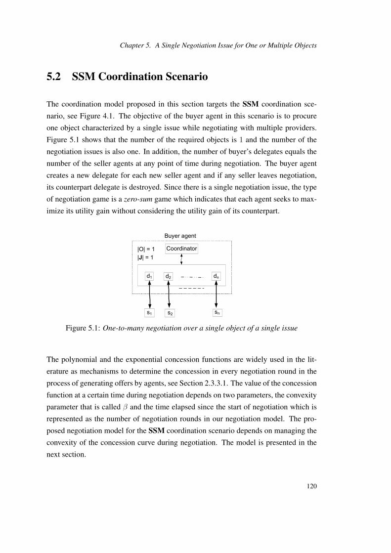
Chapter 5. A Single Negotiation Issue for One or Multiple Objects
5.2 SSM Coordination Scenario
The coordination model proposed in this section targets the SSM coordination sce-
nario, see Figure 4.1. The objective of the buyer agent in this scenario is to procure
one object characterized by a single issue while negotiating with multiple providers.
Figure 5.1 shows that the number of the required objects is 1 and the number of the
negotiation issues is also one. In addition, the number of buyer’s delegates equals the
number of the seller agents at any point of time during negotiation. The buyer agent
creates a new delegate for each new seller agent and if any seller leaves negotiation,
its counterpart delegate is destroyed. Since there is a single negotiation issue, the type
of negotiation game is a zero-sum game which indicates that each agent seeks to max-
imize its utility gain without considering the utility gain of its counterpart.
Figure 5.1: One-to-many negotiation over a single object of a single issue
The polynomial and the exponential concession functions are widely used in the lit-
erature as mechanisms to determine the concession in every negotiation round in the
process of generating offers by agents, see Section 2.3.3.1. The value of the concession
function at a certain time during negotiation depends on two parameters, the convexity
parameter that is called β and the time elapsed since the start of negotiation which is
represented as the number of negotiation rounds in our negotiation model. The pro-
posed negotiation model for the SSM coordination scenario depends on managing the
convexity of the concession curve during negotiation. The model is presented in the
next section.
120
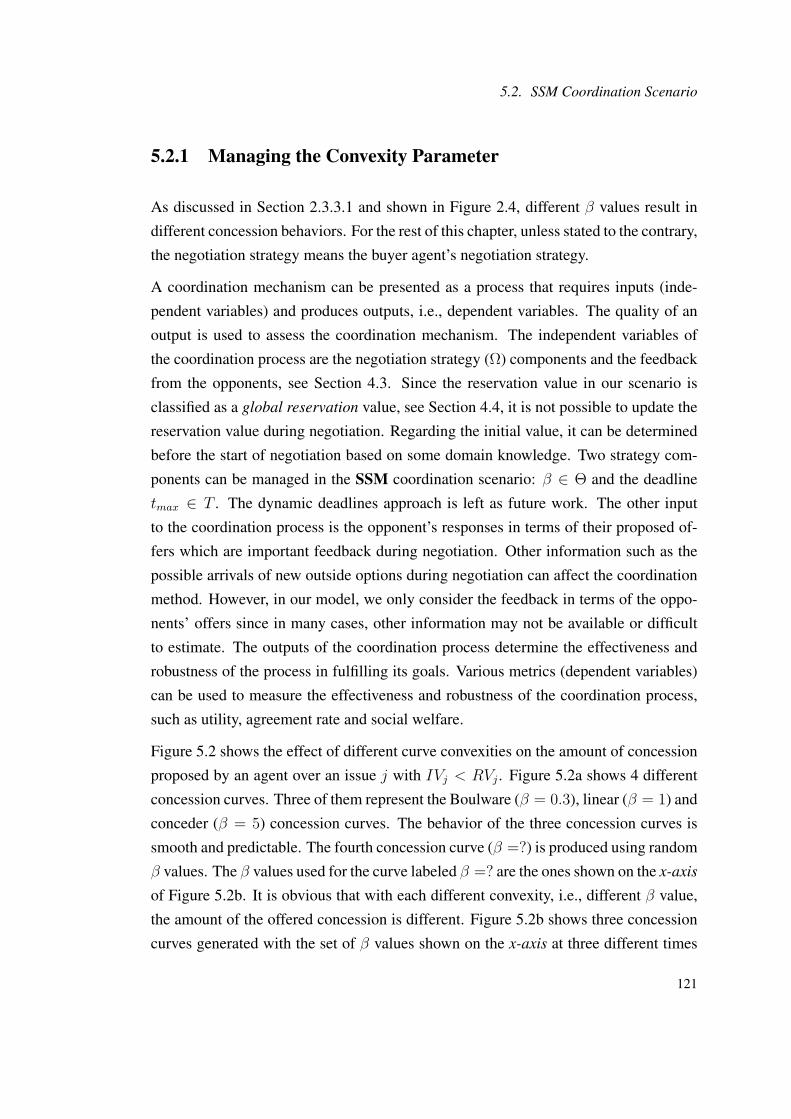
5.2. SSM Coordination Scenario
5.2.1 Managing the Convexity Parameter
As discussed in Section 2.3.3.1 and shown in Figure 2.4, different β values result in
different concession behaviors. For the rest of this chapter, unless stated to the contrary,
the negotiation strategy means the buyer agent’s negotiation strategy.
A coordination mechanism can be presented as a process that requires inputs (inde-
pendent variables) and produces outputs, i.e., dependent variables. The quality of an
output is used to assess the coordination mechanism. The independent variables of
the coordination process are the negotiation strategy (Ω) components and the feedback
from the opponents, see Section 4.3. Since the reservation value in our scenario is
classified as a global reservation value, see Section 4.4, it is not possible to update the
reservation value during negotiation. Regarding the initial value, it can be determined
before the start of negotiation based on some domain knowledge. Two strategy com-
ponents can be managed in the SSM coordination scenario: β ∈ Θ and the deadline
tmax ∈ T . The dynamic deadlines approach is left as future work. The other input
to the coordination process is the opponent’s responses in terms of their proposed of-
fers which are important feedback during negotiation. Other information such as the
possible arrivals of new outside options during negotiation can affect the coordination
method. However, in our model, we only consider the feedback in terms of the oppo-
nents’ offers since in many cases, other information may not be available or difficult
to estimate. The outputs of the coordination process determine the effectiveness and
robustness of the process in fulfilling its goals. Various metrics (dependent variables)
can be used to measure the effectiveness and robustness of the coordination process,
such as utility, agreement rate and social welfare.
Figure 5.2 shows the effect of different curve convexities on the amount of concession
proposed by an agent over an issue j with IVj < RVj . Figure 5.2a shows 4 different
concession curves. Three of them represent the Boulware (β = 0.3), linear (β = 1) and
conceder (β = 5) concession curves. The behavior of the three concession curves is
smooth and predictable. The fourth concession curve (β =?) is produced using random
β values. The β values used for the curve labeled β =? are the ones shown on the x-axis
of Figure 5.2b. It is obvious that with each different convexity, i.e., different β value,
the amount of the offered concession is different. Figure 5.2b shows three concession
curves generated with the set of β values shown on the x-axis at three different times
121
Chapter 5. A Single Negotiation Issue for One or Multiple Objects
(a) β values, different times (b) β values, time is fixed
Figure 5.2: The effect of different β values on the concession curve
where the deadline is assumed to be 20. The figure shows that at smaller times, the
amount of concession is always lower at all β values. However, at the same point of
time, different β values produce different amounts of concessions.
The idea behind the proposed coordination model (βC) is to change the value of β dur-
ing negotiation according to the collective behaviors of the in-negotiation opponents in
terms of their concessions. As mentioned is Section 4.3 and according to the assump-
tions of this thesis, there are two approaches (metrics) that can be used to evaluate the
behavior of an agent, the DIC and the LOU metrics. The DIC approach depends on the
difference in consecutive concessions of the opponents, whereas the LOU depends on
the utility value of the last offers.
When using the DIC measure to evaluate the behavior of each seller agent, the process
takes into consideration both, the concession of the seller agents and the concession
of their counterpart delegates. In some cases, the buyer’s delegates may behave dif-
ferently in terms of the amount of the concessions they are offering. Taking the be-
havior of a counterpart delegate into consideration to evaluate its opponent seller agent
is important to reach an agreement. For example, if a delegate is playing tough in
comparison to the other delegates and the opponent of that delegate is offering more
concessions than the concessions offered by the delegate but less in comparison to the
other seller agents’ concessions, then the delegate may have a slight chance of reaching
an agreement if the coordination mechanism does not consider the situation.
Ranking the seller agents according to their concessions is a possible way to compare
their behaviors, however, the problem is that ranking the seller agents can be of little
help in deciding the proper amount of concession that should be offered to each. To
122

5.2. SSM Coordination Scenario
relate the concession offered by each opponent to the concessions offered by other
opponents, the normalization process of dividing the concession offered by each seller
agent by the total concessions offered by all seller agents provide a good overview
of the concession of each seller agent in relation to the concessions offered by other
agents. The normalization process also helps in automating the process of generating
counteroffers for the next negotiation round, see Algorithm 1.
The proposed model uses the first-order differences of each agent’s offers during the
current negotiation for the first measure, while it uses the utility of the last offers re-
ceived for the second measure. The function u(xtsi→di [j]) = (maxb−xtsi→di [j])/(maxb−
minb) is used to calculate the utility of a received offer, xtsi→di [j] is the offer from a
seller si to a buyer’s thread di at time t, minb and maxb are the reservation intervals of
the buyer agent’s negotiation issue. Since agents are negotiating over a single issue, j
rather than jl (see Section 3.2) is used in this chapter to refer to the negotiation issue.
Algorithm 1 (βC)Require: Xt−1
di↔si[j], i = 1, 2, ..., n
1: for (i = 1→ n) do2: extract(Xt−1
di→si[j]))
3: extract(Xt−1si→di
[j])4: end for5: for (i = 1→ n) do . cf. Section 4.36: ∆si = (xt−1
si→si[j]− xt−2
si→si[j]), ..., (x1
si→si[j]− x0
si→si[j])
7: ∆di = (xt−1di→di
[j]− xt−2di→di
[j]), ..., (x1di→di
[j]− x0di→di
[j])8: end for9: for (i=1→ n) do
10: ∆Fi = ∆si −∆di11: end for12: ∆F = < ∆F1,∆F2, ...,∆Fn >
13: F(t1,t2)j = select(t1, t2,∆F )
14: vc = normalize(F(t1,t2)j )
15: Lut = u(Xt−1S [j])
16: vu = normalize(Lut)17: for (i = 1→ n) do18: ψti = (1− γ)vc(i) + γvu(i) . γ ∈ [0, 1]19: end for20: for (i = 1→ n) do21: βti = fβi
(ψti)22: end for23: Vβt = βtini=1
24: Return (Vβt )25: end algorithm
123
Chapter 5. A Single Negotiation Issue for One or Multiple Objects
Algorithm 1 (time complexity equals O(n)) summarizes the main steps of the algo-
rithm β coordination, βC. It evaluates the behavior of each seller agent relative to its
competitor seller agents’ behaviors at the current time t and determines the convexity
of the concession curve for each delegate accordingly. The βC strategy is executed at
the start of each negotiation round. Steps 1 to 13 in Algorithm 1 represent the data
preparation phase (see Section 4.3) that is necessary for the coordination process and
it is done at the start of every negotiation round. Steps 14 normalize the vector F (t1,t2)j .
The Lut in line 15 in Algorithm 1 stands for the utility vector of the last offers. The
symbol X(t−1)S [j] stands for the vector of the last offers received from the seller agents
in-negotiation at time (t − 1) over the issue j. The lines 17-19 find a value for each
seller agent represented by either vc or vu (vc, vu ∈ [0, 1]). The value of γ is determined
according to the importance of each measure. Steps 2 and 3 in Algorithm 1 are similar
to steps 1 and 7 in example 4.1 respectively. Steps 6 and 7 in Algorithm 1 are similar
to steps 2 and 8 in Example 4.1 respectively. Step 13 in Algorithm 1 is similar to step
17 in Example 4.1. The final output of the algorithm is the vector Vβt that has a new β
for each delegate.
A seller agent si with vtc(i) = 0 indicates that si is the most unfavorable agent in terms
of its relative concession at time t, whereas vtc(i) = 1 indicates that si is the most
favorable seller agent in terms of the amount of its relative concession at the current
time t. Accordingly, values near 1 indicate favorable seller agents and values near 0
indicate unfavorable seller agents. The same interpretation applies to the vector vu.
The function fβi(.) (line 21 in Algorithm 1) is realized in Equation 5.1. The output of
the function fβi(.), βti , is assigned to the delegate di at time t. The delegate di uses βtito generate a counteroffer to be sent to the seller agent si at time t.
fβi(ψti) =
c− cψti , ψti ∈ [0, 0.5)
max[1− ψti , ρ], ψti ∈ [0.5, 1](5.1)
At the start of negotiation, the buyer agent decides the maximum β it can use during
negotiation and assign it to c. For example, in our experiments, we use c ∈ [1, 2].
For example, if ψti = 0.4, then βti = 2 − 2 ∗ 0.4 = 1.2. When β = 1.2, the buyer
agent concedes more than when β = 0.5, for example. If ψti = 0.7, it means that
the opponent is behaving favorably, then βti = max[1 − 0.7, 0.2] = 0.3. A 0.3 β
124

5.2. SSM Coordination Scenario
value indicates that the delegate di is offering little concession at time t. The value
of the c has a significant effect on both, the utility rate and agreement rate. When the
situation is favorable to the buyer agent, the value of the c should be selected to be
small (e.g., 1 or less) to secure a high utility rate, otherwise, the value of c should be
higher to guarantee an agreement. The ρ value determines the minimum βi at time t
when ψti = 1. The value of ρ in the experiments is 0.1.
It is obvious from Equation 5.1 that the strategy choice exploits the situation and works
like a greedy algorithm. In addition, it considers both, maximizing the utility gain of an
agreement and maximizing the total number of agreements. The buyer agent chooses
to play tough with lenient opponents while playing lenient with tough opponents, see
Section 4.3. This decision reflects the buyer agent’s belief about the social behavior of
the seller agents. If the buyer has a different belief, the strategy updating mechanism
may change.
5.2.2 Experimental Results and Discussion
To evaluate the proposed βC coordination mechanism, different negotiation environ-
ments are designed to evaluate the performance of the proposed mechanism. In the
first set of experiments, the buyer agent is assumed to have the privilege of reneging
from an agreement without incurring a penalty, see Section 2.5.1. Unless stated to the
contrary, the seller agents use the (MTD) tactic (see Section 4.5.2) to generate their
offers.
The proposed strategy are benchmarked against four other strategies, namely, the des-
perate strategy (DE), the patient strategy (PA), the optimized patient strategy (OP) that
are proposed in [115] and the (eCN) strategy that is proposed in [106]. The eCN uses
historical data from previous negotiations and changes the negotiation strategy of a
buyer’s delegate after the corresponding opponent agent has been classified either as a
conceder or a non-conceder. The DE buyer agent accepts the first acceptable offer and
quits negotiation while the PA agent stays in negotiation until it reaches its deadline
then it selects the agreement with the highest utility, hence it does need to pay penalty
for reneging from all other temporary agreements. The OP buyer agent changes its
bidding strategy by changing its reservation value during negotiation. Once the OP
agent reaches a temporary agreement, it announces its new reservation value to all of
125
Chapter 5. A Single Negotiation Issue for One or Multiple Objects
its delegates since it will not accept any offer worse than the one it already has. Finally,
the eCN and the βC buyers change the convexity (by changing the β value) of their
concession curve during negotiation.
The buyer agents’ settings: five different buyer agents are being tested. Each buyer
uses a different negotiation strategy, the strategies are: βC, eCN, DE, PA and OP. All
buyer agents use the same initial settings including the deadline, the β value and the
reservation interval. In most experiments, one β value is selected randomly from the
same interval and assigned to all buyer agents. All buyer agents use the polynomial
function when adopting the time-dependent tactics to generate their counteroffers.
The minimum and the maximum values of the reservation interval of the buyer agents
are generated at the start of every negotiation instance. The minimum value is selected
randomly from the interval [5, 10] whereas the maximum value is selected randomly
from the interval [30, 50]. A negotiation instance refers to all the negotiation rounds
determined by the deadline. The end of a negotiation instance is marked by an agent
either accepting a proposal or quiting negotiation.
The seller agents’ settings: at the start of each negotiation instance, each seller agent
selects a random β value from the interval [0.5, 10]. Unless stated to the contrary, an
overlap percentage (Φj) is selected randomly from the interval [0, 1] for each seller
agent to determine the length of the overlap (agreement zone) between its reservation
interval and the reservation interval of its delegate counterpart, then the reservation
intervals are computed according to Equation 4.4.
In each negotiation instance, new five seller agents are created with different negoti-
ation parameters. All buyer agents negotiate with the same five seller agents concur-
rently. More specific negotiation settings for the buyer and the seller agents are stated
according to the objective(s) of the experiments in the following sections. Each ex-
periment is repeated 1000 times (encounters) for each buyer agent and the results are
averaged and plotted. The Mann-Whitney test [85] is used to ensure that the difference
between the βC and the best existing strategy is significant at 95% confidence level.
In addition, the error bars are shown.
126
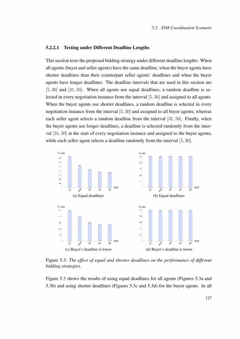
5.2. SSM Coordination Scenario
5.2.2.1 Testing under Different Deadline Lengths
This section tests the proposed bidding strategy under different deadline lengths: When
all agents (buyer and seller agents) have the same deadline, when the buyer agents have
shorter deadlines than their counterpart seller agents’ deadlines and when the buyer
agents have longer deadlines. The deadline intervals that are used in this section are
[5, 30] and [31, 50]. When all agents use equal deadlines, a random deadline is se-
lected in every negotiation instance from the interval [5, 30] and assigned to all agents.
When the buyer agents use shorter deadlines, a random deadline is selected in every
negotiation instance from the interval [5, 30] and assigned to all buyer agents, whereas
each seller agent selects a random deadline from the interval [31, 50]. Finally, when
the buyer agents use longer deadlines, a deadline is selected randomly from the inter-
val [31, 50] at the start of every negotiation instance and assigned to the buyer agents,
while each seller agent selects a deadline randomly from the interval [5, 30].
(a) Equal deadlines (b) Equal deadlines
(c) Buyer’s deadline is lower (d) Buyer’s deadline is lower
Figure 5.3: The effect of equal and shorter deadlines on the performance of differentbidding strategies.
Figure 5.3 shows the results of using equal deadlines for all agents (Figures 5.3a and
5.3b) and using shorter deadlines (Figures 5.3c and 5.3d) for the buyer agents. In all
127

Chapter 5. A Single Negotiation Issue for One or Multiple Objects
figures, A rate, U rate and BST stand for the agreement rate, the utility rate and the
buyer strategy, respectively. As Figure 5.3b shows, when all agents have the same
deadline, the agreements rate is 100% for all strategies. The reason is that all agents
offer their reservation values at their deadlines and since the agreement zones exist
between all agents, reaching an agreement is definite. When the buyer agents have
shorter deadlines, all achieve slightly lower agreement rates than in the previous case.
However, all agents achieve the same agreement rate, see Figure 5.3d. The reason is
that all buyer agents offer their reservation values (which are the same for all buyer
agents) at their deadlines and this results in achieving the same agreement rate.
Figures 5.3a and 5.3c show that the proposed βC strategy outperforms all other strate-
gies significantly in terms of the utility rate when the buyer agents and the seller agents
have equal deadlines and when the buyer agents have shorter deadlines. The eCN out-
performs the strategies OP, PA and DE significantly in terms of utility rate. The results
for the OP strategy is as expected. Since the OP buyer adjusts its reservation value
after reaching the first agreement, it is expected to reach an agreement with a higher
utility in the following negotiation rounds. Since the strategies DE and PA use the same
β value and do not change any of their negotiation parameters during negotiation, the
difference between them is not significant in terms of a utility rate. In case the buyer
agents use five different β values, the difference between the DE and the PA can be
spotted as shown in Figure 5.4.
When the buyer agents have shorter deadlines, they achieve lower utility rates than
the case when all agents have equal deadlines. The reason is that the buyer agents
offer their reservation values at their deadlines which means they offer their reser-
vation values before the seller agents do. However, the βC strategy outperforms all
other strategies significantly in terms of utility rate when the buyer agents have shorter
deadlines, see Figure 5.3c.
Figure 5.4 shows the results of testing the buyer agents’ strategies when the buyers
have longer deadlines, and when the deadlines are selected randomly for all agents. In
addition, the figure shows the results of an experiment when the buyer agents use five
different β values selected from the interval [0.5, 10] at the start of each negotiation
round. In the experiment, the same five β values are assigned to the buyer agents. The
experiment is conducted to test the difference between the DE and the PA strategies un-
128
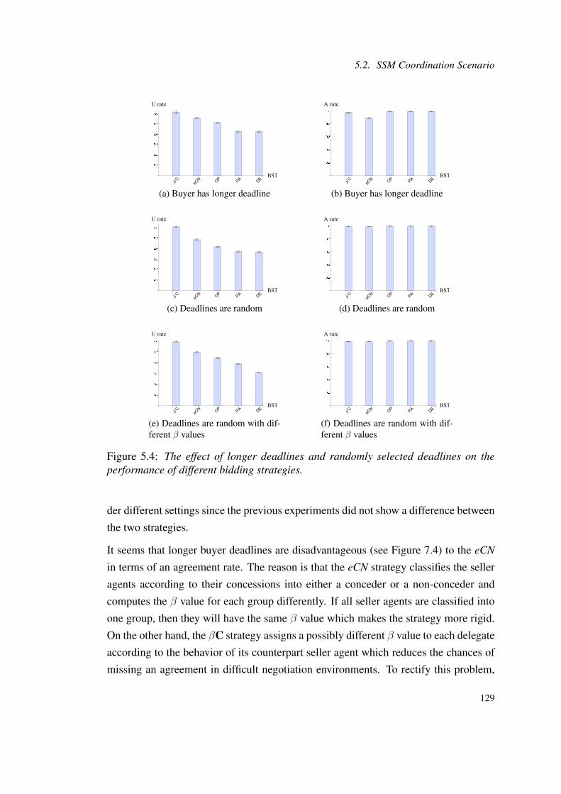
5.2. SSM Coordination Scenario
(a) Buyer has longer deadline (b) Buyer has longer deadline
(c) Deadlines are random (d) Deadlines are random
(e) Deadlines are random with dif-ferent β values
(f) Deadlines are random with dif-ferent β values
Figure 5.4: The effect of longer deadlines and randomly selected deadlines on theperformance of different bidding strategies.
der different settings since the previous experiments did not show a difference between
the two strategies.
It seems that longer buyer deadlines are disadvantageous (see Figure 7.4) to the eCN
in terms of an agreement rate. The reason is that the eCN strategy classifies the seller
agents according to their concessions into either a conceder or a non-conceder and
computes the β value for each group differently. If all seller agents are classified into
one group, then they will have the same β value which makes the strategy more rigid.
On the other hand, the βC strategy assigns a possibly different β value to each delegate
according to the behavior of its counterpart seller agent which reduces the chances of
missing an agreement in difficult negotiation environments. To rectify this problem,
129
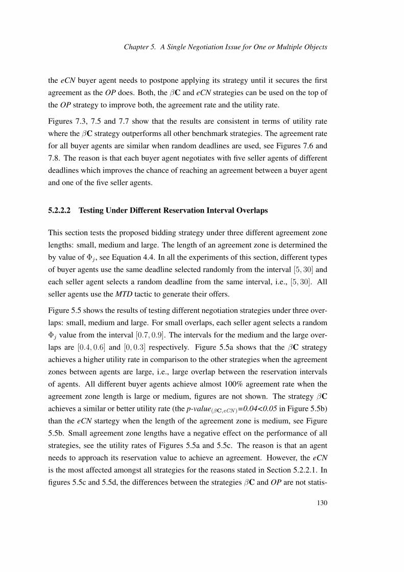
Chapter 5. A Single Negotiation Issue for One or Multiple Objects
the eCN buyer agent needs to postpone applying its strategy until it secures the first
agreement as the OP does. Both, the βC and eCN strategies can be used on the top of
the OP strategy to improve both, the agreement rate and the utility rate.
Figures 7.3, 7.5 and 7.7 show that the results are consistent in terms of utility rate
where the βC strategy outperforms all other benchmark strategies. The agreement rate
for all buyer agents are similar when random deadlines are used, see Figures 7.6 and
7.8. The reason is that each buyer agent negotiates with five seller agents of different
deadlines which improves the chance of reaching an agreement between a buyer agent
and one of the five seller agents.
5.2.2.2 Testing Under Different Reservation Interval Overlaps
This section tests the proposed bidding strategy under three different agreement zone
lengths: small, medium and large. The length of an agreement zone is determined the
by value of Φj , see Equation 4.4. In all the experiments of this section, different types
of buyer agents use the same deadline selected randomly from the interval [5, 30] and
each seller agent selects a random deadline from the same interval, i.e., [5, 30]. All
seller agents use the MTD tactic to generate their offers.
Figure 5.5 shows the results of testing different negotiation strategies under three over-
laps: small, medium and large. For small overlaps, each seller agent selects a random
Φj value from the interval [0.7, 0.9]. The intervals for the medium and the large over-
laps are [0.4, 0.6] and [0, 0.3] respectively. Figure 5.5a shows that the βC strategy
achieves a higher utility rate in comparison to the other strategies when the agreement
zones between agents are large, i.e., large overlap between the reservation intervals
of agents. All different buyer agents achieve almost 100% agreement rate when the
agreement zone length is large or medium, figures are not shown. The strategy βCachieves a similar or better utility rate (the p-value(βC,eCN )=0.04<0.05 in Figure 5.5b)
than the eCN startegy when the length of the agreement zone is medium, see Figure
5.5b. Small agreement zone lengths have a negative effect on the performance of all
strategies, see the utility rates of Figures 5.5a and 5.5c. The reason is that an agent
needs to approach its reservation value to achieve an agreement. However, the eCN
is the most affected amongst all strategies for the reasons stated in Section 5.2.2.1. In
figures 5.5c and 5.5d, the differences between the strategies βC and OP are not statis-
130

5.2. SSM Coordination Scenario
(a) Large agreement zone (b) Medium agreement zone
(c) Small agreement zone (d) Small agreement zone
Figure 5.5: The effect of different overlap percentages on the performance of differentbidding strategies.
tically significant (p-value > 0.05) in terms of both utility rate and agreement rate. The
strategies βC and eCN can be used on the top of the OP strategy, a buyer agent can
apply either the βC strategy or the eCN strategy after the first agreement is achieved to
improve both, the agreement rate and the utility rate.
5.2.2.3 Testing under Other Negotiation Environmental Conditions
In all the above experiments shown in sections 5.2.2.1 and 5.2.2.2, the buyer agents are
given the opportunity to renege from an agreement without paying penalties. However,
in many real situations, either an agent needs to honor its agreement or pay a penalty
when reneging from an agreement. To test the performance of the βC strategy under
the condition where a buyer agent needs to honor its first agreement, experiments are
conducted to test three different strategies under random deadlines and random over-
laps. The PA and the OP strategies do not apply in this case. The strategies PA and
OP assume that a buyer agent has the privilege of reneging on an agreement(s) without
paying penalty.
131
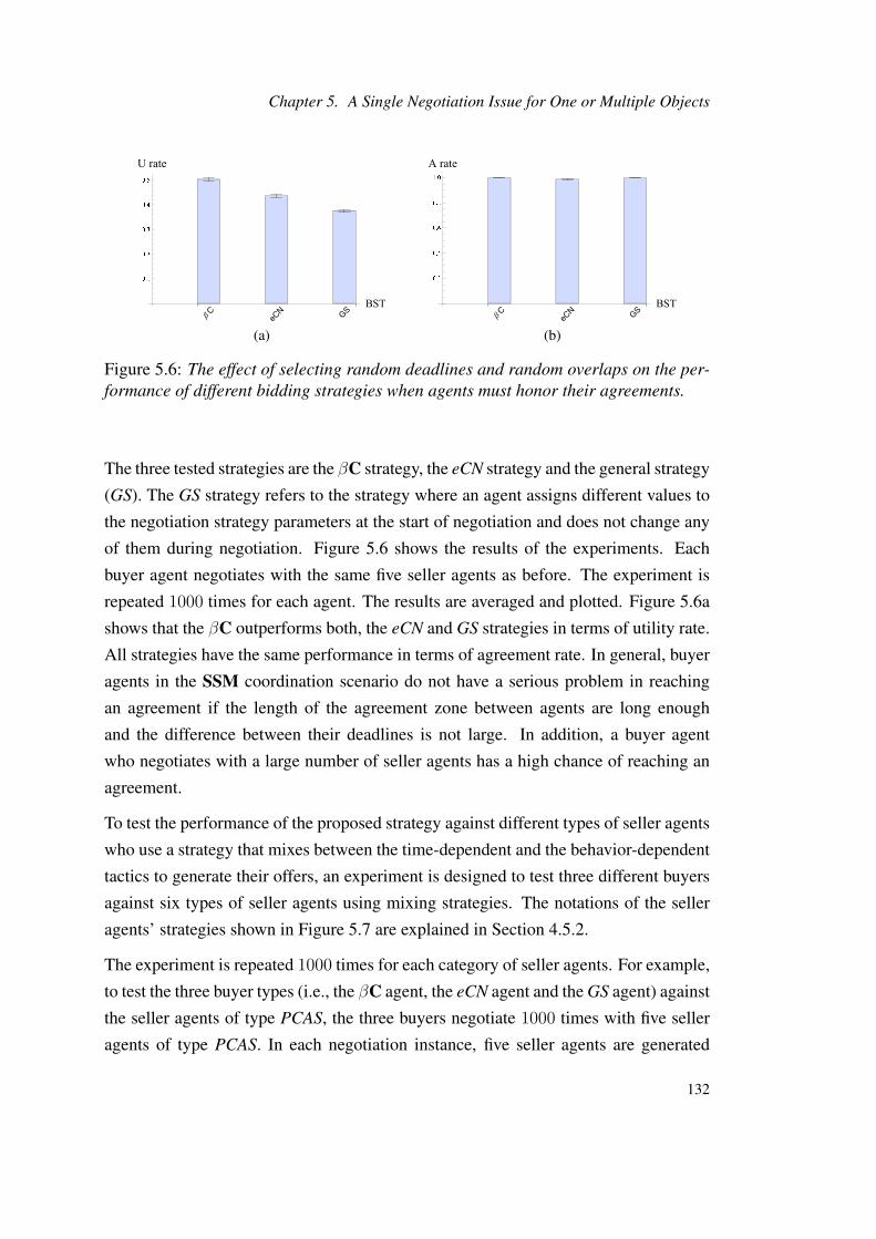
Chapter 5. A Single Negotiation Issue for One or Multiple Objects
(a) (b)
Figure 5.6: The effect of selecting random deadlines and random overlaps on the per-formance of different bidding strategies when agents must honor their agreements.
The three tested strategies are the βC strategy, the eCN strategy and the general strategy
(GS). The GS strategy refers to the strategy where an agent assigns different values to
the negotiation strategy parameters at the start of negotiation and does not change any
of them during negotiation. Figure 5.6 shows the results of the experiments. Each
buyer agent negotiates with the same five seller agents as before. The experiment is
repeated 1000 times for each agent. The results are averaged and plotted. Figure 5.6a
shows that the βC outperforms both, the eCN and GS strategies in terms of utility rate.
All strategies have the same performance in terms of agreement rate. In general, buyer
agents in the SSM coordination scenario do not have a serious problem in reaching
an agreement if the length of the agreement zone between agents are long enough
and the difference between their deadlines is not large. In addition, a buyer agent
who negotiates with a large number of seller agents has a high chance of reaching an
agreement.
To test the performance of the proposed strategy against different types of seller agents
who use a strategy that mixes between the time-dependent and the behavior-dependent
tactics to generate their offers, an experiment is designed to test three different buyers
against six types of seller agents using mixing strategies. The notations of the seller
agents’ strategies shown in Figure 5.7 are explained in Section 4.5.2.
The experiment is repeated 1000 times for each category of seller agents. For example,
to test the three buyer types (i.e., the βC agent, the eCN agent and the GS agent) against
the seller agents of type PCAS, the three buyers negotiate 1000 times with five seller
agents of type PCAS. In each negotiation instance, five seller agents are generated
132

5.2. SSM Coordination Scenario
(a) (b)
(1→ βC, 2→ eCN , 3→ GS )
Figure 5.7: Seller agents mix between the time-dependent and the behavior-dependenttactics where all agents need to honor their agreements.
randomly from the PCAS category and the three buyer types negotiate with the same
five agents. The results are averaged and plotted. Random deadlines and overlaps are
used at the start of each negotiation instance. All buyer agents have the same deadline
in every negotiation instance. Finally, a β value is selected randomly from the interval
[0.5, 10] and assigned to the three buyer agents. The same process is repeated for the
rest of the five categories of the seller agents.
Figure 5.7b shows that the three different buyer types record similar agreement rates.
On the other hand, the βC strategy outperforms (with significant statistical differ-
ence) the other two strategies in terms of the utility rate in all cases, see Figure 5.7a.
When the seller agents are selected from the PCAS and the PCAM categories, all buyer
agent types achieve lower utility rates than the utility rates achieved when the buyer
agents negotiate against the seller agents of the types PLAS, PLAM, PBAS, and PBAM.
The reason is that the seller agents in the PCAS and the PCAM categories are time-
dependent conceder types and since the contribution of the behavior-dependent is small
to medium (see Section 4.5.2), the sellers are conceding quickly which means that the
buyer agents reach agreements with higher utility rates. The experiments that consider
testing the different negotiation strategies against sellers using mixing strategies prove
that the proposed βC strategy is a dynamic strategy that responds to different negotia-
tion environments and different opponent types in an effective and robust manner.
133
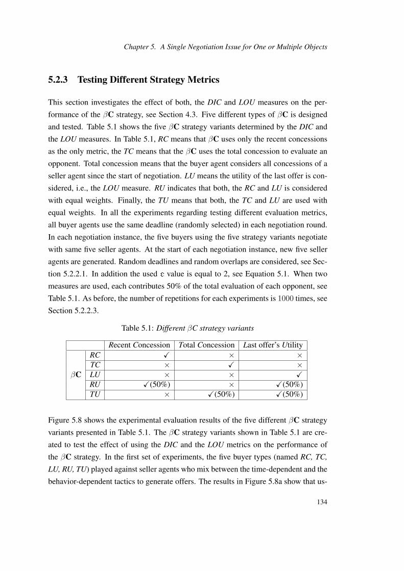
Chapter 5. A Single Negotiation Issue for One or Multiple Objects
5.2.3 Testing Different Strategy Metrics
This section investigates the effect of both, the DIC and LOU measures on the per-
formance of the βC strategy, see Section 4.3. Five different types of βC is designed
and tested. Table 5.1 shows the five βC strategy variants determined by the DIC and
the LOU measures. In Table 5.1, RC means that βC uses only the recent concessions
as the only metric, the TC means that the βC uses the total concession to evaluate an
opponent. Total concession means that the buyer agent considers all concessions of a
seller agent since the start of negotiation. LU means the utility of the last offer is con-
sidered, i.e., the LOU measure. RU indicates that both, the RC and LU is considered
with equal weights. Finally, the TU means that both, the TC and LU are used with
equal weights. In all the experiments regarding testing different evaluation metrics,
all buyer agents use the same deadline (randomly selected) in each negotiation round.
In each negotiation instance, the five buyers using the five strategy variants negotiate
with same five seller agents. At the start of each negotiation instance, new five seller
agents are generated. Random deadlines and random overlaps are considered, see Sec-
tion 5.2.2.1. In addition the used c value is equal to 2, see Equation 5.1. When two
measures are used, each contributes 50% of the total evaluation of each opponent, see
Table 5.1. As before, the number of repetitions for each experiments is 1000 times, see
Section 5.2.2.3.
Table 5.1: Different βC strategy variants
Recent Concession Total Concession Last offer’s Utility
βC
RC X × ×TC × X ×LU × × XRU X(50%) × X(50%)TU × X(50%) X(50%)
Figure 5.8 shows the experimental evaluation results of the five different βC strategy
variants presented in Table 5.1. The βC strategy variants shown in Table 5.1 are cre-
ated to test the effect of using the DIC and the LOU metrics on the performance of
the βC strategy. In the first set of experiments, the five buyer types (named RC, TC,
LU, RU, TU) played against seller agents who mix between the time-dependent and the
behavior-dependent tactics to generate offers. The results in Figure 5.8a show that us-
134
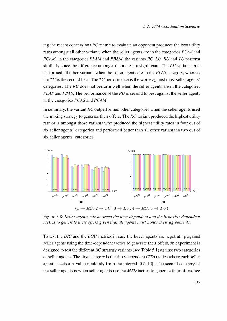
5.2. SSM Coordination Scenario
ing the recent concessions RC metric to evaluate an opponent produces the best utility
rates amongst all other variants when the seller agents are in the categories PCAS and
PCAM. In the categories PLAM and PBAM, the variants RC, LU, RU and TU perform
similarly since the difference amongst them are not significant. The LU variants out-
performed all other variants when the seller agents are in the PLAS category, whereas
the TU is the second best. The TC performance is the worse against most seller agents’
categories. The RC does not perform well when the seller agents are in the categories
PLAS and PBAS. The performance of the RU is second to best against the seller agents
in the categories PCAS and PCAM.
In summary, the variant RC outperformed other categories when the seller agents used
the mixing strategy to generate their offers. The RC variant produced the highest utility
rate or is amongst those variants who produced the highest utility rates in four out of
six seller agents’ categories and performed better than all other variants in two out of
six seller agents’ categories.
(a) (b)
(1→ RC, 2→ TC, 3→ LU , 4→ RU , 5→ TU )
Figure 5.8: Seller agents mix between the time-dependent and the behavior-dependenttactics to generate their offers given that all agents must honor their agreements.
To test the DIC and the LOU metrics in case the buyer agents are negotiating against
seller agents using the time-dependent tactics to generate their offers, an experiment is
designed to test the different βC strategy variants (see Table 5.1) against two categories
of seller agents. The first category is the time-dependent (TD) tactics where each seller
agent selects a β value randomly from the interval [0.5, 10]. The second category of
the seller agents is when seller agents use the MTD tactics to generate their offers, see
135
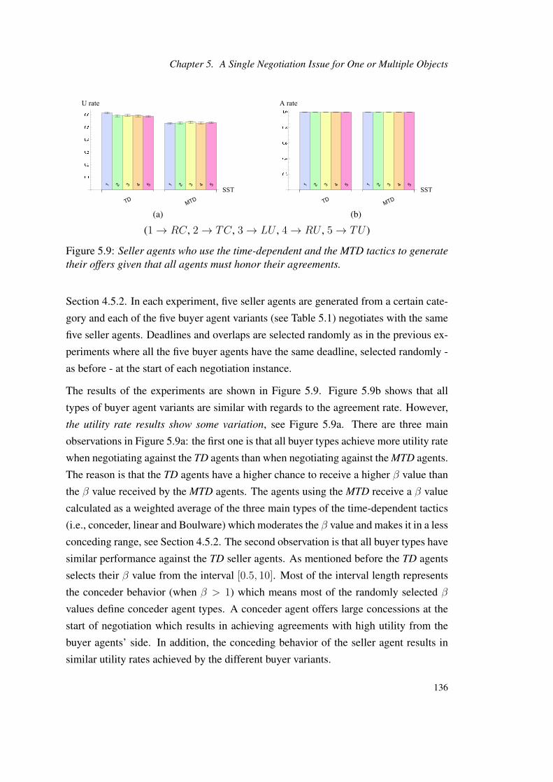
Chapter 5. A Single Negotiation Issue for One or Multiple Objects
(a) (b)
(1→ RC, 2→ TC, 3→ LU , 4→ RU , 5→ TU )
Figure 5.9: Seller agents who use the time-dependent and the MTD tactics to generatetheir offers given that all agents must honor their agreements.
Section 4.5.2. In each experiment, five seller agents are generated from a certain cate-
gory and each of the five buyer agent variants (see Table 5.1) negotiates with the same
five seller agents. Deadlines and overlaps are selected randomly as in the previous ex-
periments where all the five buyer agents have the same deadline, selected randomly -
as before - at the start of each negotiation instance.
The results of the experiments are shown in Figure 5.9. Figure 5.9b shows that all
types of buyer agent variants are similar with regards to the agreement rate. However,
the utility rate results show some variation, see Figure 5.9a. There are three main
observations in Figure 5.9a: the first one is that all buyer types achieve more utility rate
when negotiating against the TD agents than when negotiating against the MTD agents.
The reason is that the TD agents have a higher chance to receive a higher β value than
the β value received by the MTD agents. The agents using the MTD receive a β value
calculated as a weighted average of the three main types of the time-dependent tactics
(i.e., conceder, linear and Boulware) which moderates the β value and makes it in a less
conceding range, see Section 4.5.2. The second observation is that all buyer types have
similar performance against the TD seller agents. As mentioned before the TD agents
selects their β value from the interval [0.5, 10]. Most of the interval length represents
the conceder behavior (when β > 1) which means most of the randomly selected β
values define conceder agent types. A conceder agent offers large concessions at the
start of negotiation which results in achieving agreements with high utility from the
buyer agents’ side. In addition, the conceding behavior of the seller agent results in
similar utility rates achieved by the different buyer variants.
136
5.3. MSM Coordination Scenario
The third observation is that when the buyer agent variants negotiate against the TD,
the RC performs better than the other variables while if the seller agents are of type
MTD, all buyer variants perform similarly.
In most cases, the RC metric is proved to be a better evaluation criterion than the TC
metric. The total concessions for two agents can be the same at a certain point in time
during negotiation even if the two agents are offering different amounts of concessions
at different times. For example, assume that agents a1 and a2 are in negotiation and
agent a1 concedes 2 units every round and agent a2 concedes 1 unit every round. After
9 negotiation rounds, the total amount of concessions of agent a1 is 18 units and the
total amounts of concessions of agent a2 is 9 units. At the next negotiation round,
agent a1 concedes 2 units and agent a2 concedes 11 units. The two agents offered
the same amount of concession in total in the negotiation round number 10. It can be
guessed that agent a2 is more desperate to reach an agreement than a1. In addition,
the recent concession metric is proved to be similar or better than the utility metric in
most cases. The reason is that the utility measures the current value of an opponent
agent without considering its previous behavior in terms of the concession offered. The
recent concession considers the most recent behaviors of all agents which can evaluate
them more accurately.
Even though the RU metric is used in the experiments of Section 5.2.2, the RU metric
performs better than all other benchmark strategies. In the future experiments, the RC
metric will be considered.
5.3 MSM Coordination Scenario
This section presents coordination mechanisms that are designed to coordinate the
bidding strategy for the MSM coordination scenario where a buyer agent is negotiating
with seller agents over multiple distinct objects given that each object has a single
negotiation issue and multiple providers, see Figure 5.10.
Procuring more than one negotiation object is a daily practice of buyers who use either
physical stores or virtual stores. We investigate the situation where a buyer agent is ne-
gotiating with multiple seller agents concurrently for the purpose of reaching multiple
agreements over multiple objects, i.e., one agreement per one object. For example, in
137

Chapter 5. A Single Negotiation Issue for One or Multiple Objects
service composition, a buyer agent may negotiate over multiple distinct services where
each service has multiple providers.
Figure 5.10: One-to-many negotiation over multiple negotiation objects of one issue
There are two levels of coordination shown in Figure 5.10. The first level is referred to
as global coordination while the second one is called local coordination. The global
coordination considers the overall situation of negotiation taking into consideration the
common factor(s) in the given coordination scenario. There are two common factors
in our scenario: the first one is that all objects have the same issue, i.e., the negotiation
issue is common amongst all objects, e.g., price. The second factor is that the agree-
ments are connected. Thus if a negotiation over an object results in failure regarding
any object, the whole negotiation process fails.
The local coordination indicates that the coordination mechanism(s) considers the ne-
gotiation situation with regards to a certain object without considering the negotiation
situation of other objects. The proposed coordination mechanism considers the num-
ber and behaviors of the seller agents of a certain object in terms of their concessions
in comparison to the concessions offered by their counterpart delegates. In all coordi-
nation mechanisms proposed in this thesis, only those sellers that are still negotiating
are considered. If a seller quits negotiation, it is dropped from the analysis process.
This section presents three coordination mechanisms classified according to the co-
ordination scope: a global MSM mechanism (GMSM), a local MSM mechanism
(LMSM) and finally a hybrid (MSM) mechanism (HMSM). In all the experimen-
tal results shown in this section, all agents honor their first agreement. Unless stated to
the contrary, all seller agents use the MTD tactic to generate their offers.
138

5.3. MSM Coordination Scenario
5.3.1 Global MSM Strategy
The proposed global negotiation strategy considers assignment of possibly new lo-
cal reservation values (see Section 4.4) to the negotiation issue(s) in each negotiation
round. The assignment of a new local reservation value for each negotiation issue
of each object depends on both the values of consecutive offers received from each
provider of each object and their counterpart delegates’ consecutive counteroffers. Al-
gorithm 2 summarizes the main steps of the GMSM mechanism. Each object is as-
signed a weight that determines its issue’s local reservation value. For example, if
the weight vector for four objects is w = 0.3, 0.2, 0.4, 0.1 and the global reserva-
tion value is $100, then the local reservation values are 30, 20, 40, 10. The initial
weight vector is assigned based either on domain knowledge or previous negotiation
experience.
The lines 1-5 in Algorithm 2 assign a zero weight for each procured object and then
recompute the weights for the remaining objects in line 6. The data preparation process
presented in lines 7-13 is similar to the data preparation process shown in Algorithm 1.
The difference is that the data process of Algorithm 1 considers one negotiation object
while the data preparation process shown in Algorithm 2 considers multiple objects
and m in the algorithm stands for the number of negotiation objects required by the
buyer agent, see Figure 5.10. Line 14 computes the mean vector for the vector F (t1,t2)j
(see Section 4.3) while line 15 normalizes the mean vector that results in relating the
behaviors of the seller agent groups to each other by dividing the value of each member
in the vector by the sum of the vector. The normalization process in the given context
provides a value for each group of seller agents relative to the other seller agent groups.
An example of the vector F (t1,t2)j , F (t1,t2)
j =< <1,2,3>,<-1,0,3>,<2,4>,<5> >. In this
case, the number of the required objects is 4. The element <1,2,3> represents the dif-
ference between the first order differences of the concessions offered by the providers
and the concessions offered by their counterpart delegates in the previous negotiation
round over the negotiation issue j of object 1.
The element < 2, 4 > represents the same information for two pairs of agents which
indicates that one of the object 3 providers withdrew from negotiation and only two
providers are left. For object number 4, there is only one provider left.
139
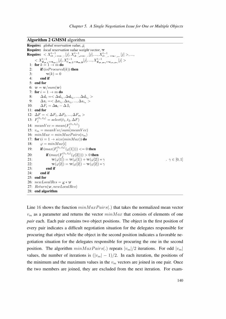
Chapter 5. A Single Negotiation Issue for One or Multiple Objects
Algorithm 2 GMSM algorithmRequire: global reservation value, gRequire: local reservation value weight vector, wRequire: < Xt−1
d1,1↔s1,1[j], Xt−1
d1,2↔s1,2[j], ..., Xt−1
d1,n1↔s1,n1
[j] >, ...,
< Xt−1dm,1↔sm,1
[j], Xt−1dm,2↔sm,2
[j], ..., Xt−1dm,mn↔sm,mn
[j] >1: for k = 1→ m do2: if (isProcured(k)) then3: w(k) = 04: end if5: end for6: w = w/sum(w)7: for i = 1→ m do8: ∆di =< ∆di1 ,∆di2 , ...,∆din >9: ∆si =< ∆si1 ,∆si2 , ...,∆sin >
10: ∆Fi = ∆si −∆di11: end for12: ∆F = < ∆F1,∆F2, ...,∆Fm >
13: F(t1,t2)j = select(t1, t2,∆F )
14: meanV ec = mean(F(t1,t2)j )
15: vm = meanV ec/sum(meanV ec)16: minMax = minMaxPairs(vm)17: for (i = 1→ size(minMax)) do18: ϕ = minMax[i]
19: if (max(F(t1,t2)j (ϕ[1]))) <= 0 then
20: if (max(F(t1,t2)j (ϕ[2]))) > 0 then
21: w(ϕ[1]) = w(ϕ[1]) +w(ϕ[2]) ∗ γ . γ ∈ [0, 1]22: w(ϕ[2]) = w(ϕ[2])−w(ϕ[2]) ∗ γ23: end if24: end if25: end for26: newLocalRes = g ∗w27: Return(w, newLocalRes)28: end algorithm
Line 16 shows the function minMaxPairs(.) that takes the normalized mean vector
vm as a parameter and returns the vector minMax that consists of elements of one
pair each. Each pair contains two object positions. The object in the first position of
every pair indicates a difficult negotiation situation for the delegates responsible for
procuring that object while the object in the second position indicates a favorable ne-
gotiation situation for the delegates responsible for procuring the one in the second
position. The algorithm minMaxPairs(.) repeats |vm|/2 iterations. For odd |vm|values, the number of iterations is (|vm| − 1)/2. In each iteration, the positions of
the minimum and the maximum values in the vm vectors are joined in one pair. Once
the two members are joined, they are excluded from the next iteration. For exam-
140
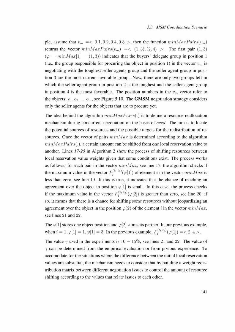
5.3. MSM Coordination Scenario
ple, assume that vm =< 0.1, 0.2, 0.4, 0.3 >, then the function minMaxPairs(vm)
returns the vector minMaxPairs(vm) =< (1, 3), (2, 4) >. The first pair (1, 3)
(ϕ = minMax[1] = (1, 3)) indicates that the buyers’ delegate group in position 1
(i.e., the group responsible for procuring the object in position 1) in the vector vm is
negotiating with the toughest seller agents group and the seller agent group in posi-
tion 3 are the most current favorable group. Now, there are only two groups left in
which the seller agent group in position 2 is the toughest and the seller agent group
in position 4 is the most favorable. The position numbers in the vm vector refer to
the objects: o1, o2, ..., om, see Figure 5.10. The GMSM negotiation strategy considers
only the seller agents for the objects that are to procure yet.
The idea behind the algorithm minMaxPairs(.) is to define a resource reallocation
mechanism during concurrent negotiation on the bases of need. The aim is to locate
the potential sources of resources and the possible targets for the redistribution of re-
sources. Once the vector of pairs minMax is determined according to the algorithm
minMaxPairs(.), a certain amount can be shifted from one local reservation value to
another. Lines 17-25 in Algorithm 2 show the process of shifting resources between
local reservation value weights given that some conditions exist. The process works
as follows: for each pair in the vector minMax, see line 17, the algorithm checks if
the maximum value in the vector F (t1,t2)j (ϕ[1]) of element i in the vector minMax is
less than zero, see line 19. If this is true, it indicates that the chance of reaching an
agreement over the object in position ϕ[1] is small. In this case, the process checks
if the maximum value in the vector F (t1,t2)j (ϕ[2]) is greater than zero, see line 20; if
so, it means that there is a chance for shifting some resources without jeopardizing an
agreement over the object in the position ϕ(2) of the element i in the vector minMax,
see lines 21 and 22.
The ϕ[1] stores one object position and ϕ[2] stores its partner. In our previous example,
when i = 1, ϕ[1] = 1, ϕ[1] = 3. In the previous example, F (t1,t2)j (ϕ[1]) =< 2, 4 >.
The value γ used in the experiments is 10 − 15%, see lines 21 and 22. The value of
γ can be determined from the empirical evaluation or from prvious experience. To
accomodate for the situations where the difference between the initial local reservation
values are substatial, the mechanism needs to consider that by building a weight redis-
tribution matrix between different negotiation issues to control the amount of resource
shifting according to the values that relate issues to each other.
141
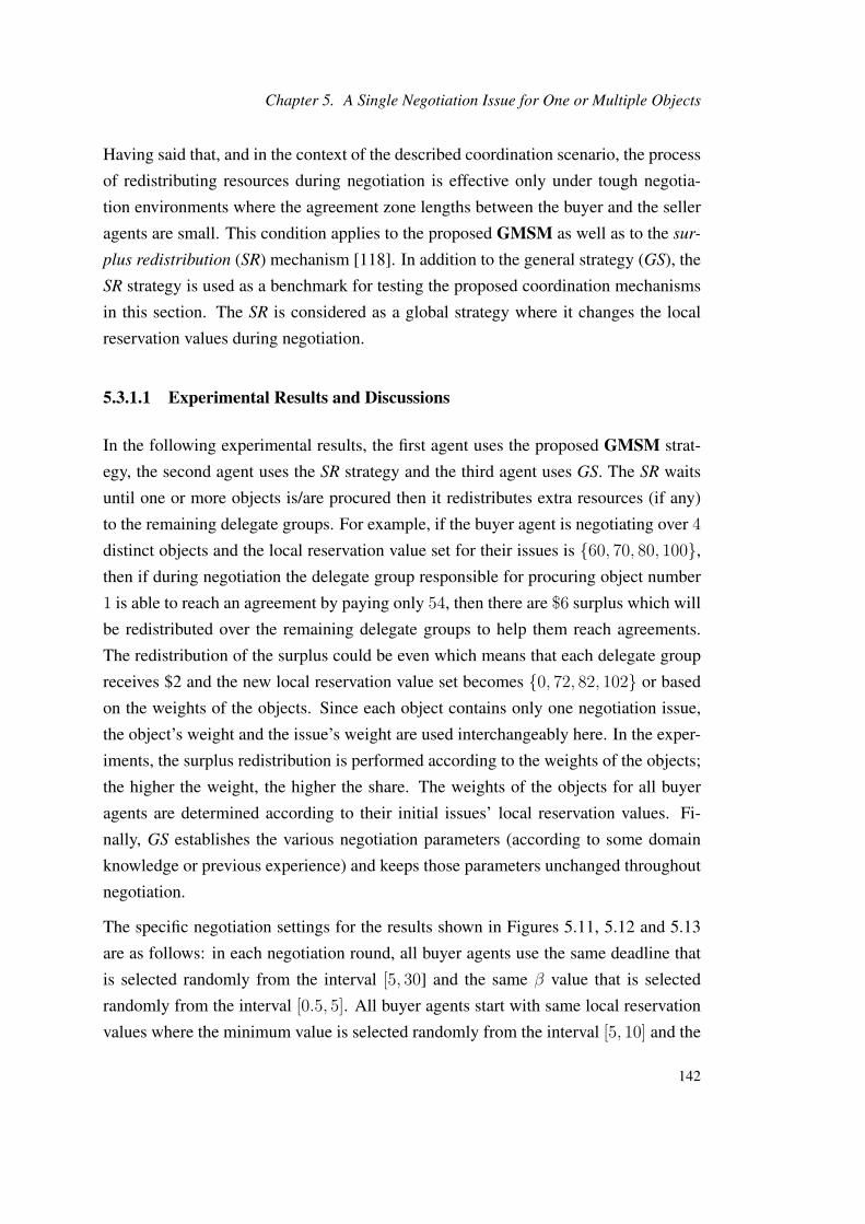
Chapter 5. A Single Negotiation Issue for One or Multiple Objects
Having said that, and in the context of the described coordination scenario, the process
of redistributing resources during negotiation is effective only under tough negotia-
tion environments where the agreement zone lengths between the buyer and the seller
agents are small. This condition applies to the proposed GMSM as well as to the sur-
plus redistribution (SR) mechanism [118]. In addition to the general strategy (GS), the
SR strategy is used as a benchmark for testing the proposed coordination mechanisms
in this section. The SR is considered as a global strategy where it changes the local
reservation values during negotiation.
5.3.1.1 Experimental Results and Discussions
In the following experimental results, the first agent uses the proposed GMSM strat-
egy, the second agent uses the SR strategy and the third agent uses GS. The SR waits
until one or more objects is/are procured then it redistributes extra resources (if any)
to the remaining delegate groups. For example, if the buyer agent is negotiating over 4
distinct objects and the local reservation value set for their issues is 60, 70, 80, 100,then if during negotiation the delegate group responsible for procuring object number
1 is able to reach an agreement by paying only 54, then there are $6 surplus which will
be redistributed over the remaining delegate groups to help them reach agreements.
The redistribution of the surplus could be even which means that each delegate group
receives $2 and the new local reservation value set becomes 0, 72, 82, 102 or based
on the weights of the objects. Since each object contains only one negotiation issue,
the object’s weight and the issue’s weight are used interchangeably here. In the exper-
iments, the surplus redistribution is performed according to the weights of the objects;
the higher the weight, the higher the share. The weights of the objects for all buyer
agents are determined according to their initial issues’ local reservation values. Fi-
nally, GS establishes the various negotiation parameters (according to some domain
knowledge or previous experience) and keeps those parameters unchanged throughout
negotiation.
The specific negotiation settings for the results shown in Figures 5.11, 5.12 and 5.13
are as follows: in each negotiation round, all buyer agents use the same deadline that
is selected randomly from the interval [5, 30] and the same β value that is selected
randomly from the interval [0.5, 5]. All buyer agents start with same local reservation
values where the minimum value is selected randomly from the interval [5, 10] and the
142

5.3. MSM Coordination Scenario
maximum value is selected randomly from the interval [40, 50] in every negotiation
round. Each seller agent selects a random deadline from the same interval, i.e.,[5, 30]
and a random β value from the interval [0.5, 10]. In addition, the percentages of over-
laps between the local reservation values of the agents’ issue are selected randomly
from the interval [0.9, 1] which means that any overlap percentage will be %10 or less,
see Equation 4.4. Unless stated to the contrary, the number of negotiation objects used
in the experiments of this section is 10.
(a) (b)
(1→ GMSM , 2→ SR, 3→ GS)(The numbers above the graph bars refer to the number of seller agents per object)
Figure 5.11: Testing the strategies GMSM, SR and GS; number of seller agents varies
The first experimental results are shown in Figure 5.11. The numbers above the bars in
Figures 5.11 and 5.12 indicate the number of seller agents per object. For each distinct
number of agents, the experiment is repeated 1000 times and the results are averaged
and plotted. The experiment starts with 2 agents per object and the number increases
until it reaches 10 seller agents per object. The results show that when the number
of seller agents is relatively small, the proposed GMSM strategy outperforms the SR
strategy significantly in terms of agreement rate and equal or better in terms of utility
rate. Both, the GMSM and SR outperform GS significantly in all cases, see Figures
5.11a and 5.11b.
Anther set of experiments show that when the overlap percentages between the agents’
reservation intervals are %5 or less, the GMSM strategy proves to have even more sig-
nificant performance than the SR strategy in terms of agreement rate, see Figure 5.12b.
Figure 5.12a shows that the GMSM strategy performs better than the SR strategy in
143
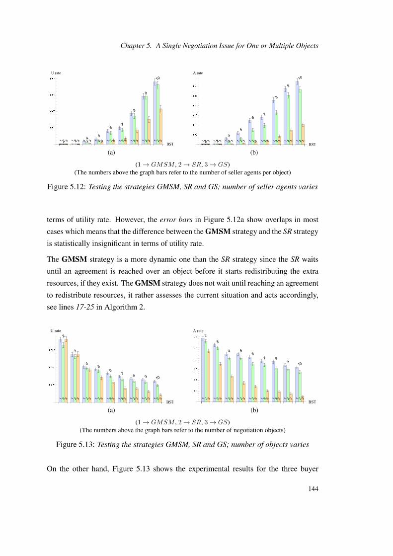
Chapter 5. A Single Negotiation Issue for One or Multiple Objects
(a) (b)
(1→ GMSM , 2→ SR, 3→ GS)(The numbers above the graph bars refer to the number of seller agents per object)
Figure 5.12: Testing the strategies GMSM, SR and GS; number of seller agents varies
terms of utility rate. However, the error bars in Figure 5.12a show overlaps in most
cases which means that the difference between the GMSM strategy and the SR strategy
is statistically insignificant in terms of utility rate.
The GMSM strategy is a more dynamic one than the SR strategy since the SR waits
until an agreement is reached over an object before it starts redistributing the extra
resources, if they exist. The GMSM strategy does not wait until reaching an agreement
to redistribute resources, it rather assesses the current situation and acts accordingly,
see lines 17-25 in Algorithm 2.
(a) (b)
(1→ GMSM , 2→ SR, 3→ GS)(The numbers above the graph bars refer to the number of negotiation objects)
Figure 5.13: Testing the strategies GMSM, SR and GS; number of objects varies
On the other hand, Figure 5.13 shows the experimental results for the three buyer
144

5.3. MSM Coordination Scenario
agents negotiating against 5 seller agents over different number of objects. The num-
bers above the bars in the figure indicate the number of negotiation objects. The num-
ber starts with 2 distinct objects and increases up to 10 objects. When the number of
objects increases, the GMSM strategy outperforms the other two strategies in terms of
utility rate and agreement rate, see Figures 5.13a and 5.13b. Both dynamic strategies
outperform GS in terms of utility rate and agreement rate when the number of objects
becomes large. When the number of objects becomes large, it becomes difficult for all
strategies to reach a large number of agreements. However, GMSM proved to be more
effective than the SR strategy especially when the number of objects becomes large.
Figure 5.14 shows the experimental results when the three buyer agents are negotiating
against seller agents who mix between the time-dependent tactics and the behavior-
dependent tactics to generate their offers, see Section 4.5.2. In most cases, the GMSMoutperforms the SR strategy in terms of utility rate and agreement rate, see Figures
5.14a and 5.14b. GS shows a better utility rate than the other two strategies in case the
seller agents are selected from the type PBAS. The reason is that the seller agents in
the type PBAS use the Boulware tactic to generate their offers which constitute large
portion of their final mixed offers, while the contribution of the behavior-dependent
strategy is small, see Section 4.5.2.
(a) (b)
(1→ GMSM , 2→ SR, 3→ GS)
Figure 5.14: Testing the strategies GMSM, SR and GS; the seller agents mix betweenthe time-dependent tactics and the behavior dependent tactics to generate their offers
When all the seller agents are of Boulware type, they offer little concessions throughout
negotiation until they approach their deadlines in which they offer large concessions.
In this case and because the two dynamic strategies shift resources during negotiation,
145
Chapter 5. A Single Negotiation Issue for One or Multiple Objects
the utility of an agreement is expected to be low. Figure 5.14b shows that the two
dynamic strategies outperform GS in terms of utility rate and significantly in all cases
in terms of agreement rate. The percentage of overlaps used in the experiments of
Figure 5.14 are selected randomly to be 30% or less. The rest of the experimental
settings are the same as in the experiments used to generate the previous results in this
section.
When the length of the agreement zone between agents is small, a small utility is ex-
pected for an agreement. The results of utility rate show this in all figures of this chap-
ter, e.g., Figures 5.11, 5.12 and 5.13. The reason is that, since the overlap percentages
between the reservation intervals of the buyer agents and the seller agents are small, all
agents need to approach their reservation values before reaching the agreement zone
which results in low utility rate outcomes for all agents.
5.3.2 Local and Hybrid MSM Strategies
The proposed local negotiation strategy (LMSM) considers only the negotiation situa-
tion regarding each object alone, hence the name local. The LMSM strategy does not
require the existence of common factors such as common issues. It interacts with the
providers of each object in isolation and aims at reaching a high utility agreement.
The strategy decides the convexity of the concession curve for each group of delegates
in each negotiation round taking into consideration the behaviors and the number of
seller agents of a certain object without considering the behaviors or the number of
seller agents for the other objects. The LMSM strategy depends on the number of the
existing seller agents who behave favorably in terms of their concessions compared to
their counterpart delegates’ concessions. If the number of favorable agents is beyond
a certain ε threshold, then the strategy chooses a tough negotiation stance or otherwise
it chooses either a linear or a conceder stance. Algorithm 3 outlines the proposed
mechanism. The algorithm iterates m times which is equivalent to the number of
negotiation objects. In each iteration the data preparation process is first executed (lines
1-6) then the conditional if-statement is used to count the number of existing seller
agents who offered more concessions than their counterpart delegates’ concessions in
the previous negotiation round, see lines 7-24.
146
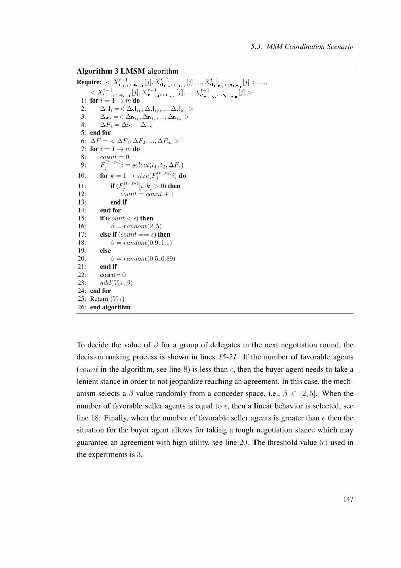
5.3. MSM Coordination Scenario
Algorithm 3 LMSM algorithmRequire: < Xt−1
d1,1↔s1,1[j], Xt−1
d1,2↔s1,2[j], ..., Xt−1
d1,n1↔s1,n1[j] >, ...,
< Xt−1dm,1↔sm,1
[j], Xt−1dm,2↔sm,2
[j], ..., Xt−1dm,mn↔sm,mn
[j] >1: for i = 1→ m do2: ∆di =< ∆di1 ,∆di2 , ...,∆din >3: ∆si =< ∆si1 ,∆si2 , ...,∆sin >4: ∆Fi = ∆si −∆di5: end for6: ∆F = < ∆F1,∆F2, ...,∆Fm >7: for i = 1→ m do8: count = 09: F
(t1,t2)j i = select(t1, t2,∆Fi)
10: for k = 1→ size(F(t1,t2)j i) do
11: if (F (t1,t2)j [i, k] > 0) then
12: count = count+ 113: end if14: end for15: if (count < ε) then16: β = random(2, 5)17: else if (count == ε) then18: β = random(0.9, 1.1)19: else20: β = random(0.5, 0.89)21: end if22: count = 023: add(Vβt , β)24: end for25: Return (Vβt )26: end algorithm
To decide the value of β for a group of delegates in the next negotiation round, the
decision making process is shown in lines 15-21. If the number of favorable agents
(count in the algorithm, see line 8) is less than ε, then the buyer agent needs to take a
lenient stance in order to not jeopardize reaching an agreement. In this case, the mech-
anism selects a β value randomly from a conceder space, i.e., β ∈ [2, 5]. When the
number of favorable seller agents is equal to ε, then a linear behavior is selected, see
line 18. Finally, when the number of favorable seller agents is greater than ε then the
situation for the buyer agent allows for taking a tough negotiation stance which may
guarantee an agreement with high utility, see line 20. The threshold value (ε) used in
the experiments is 3.
147

Chapter 5. A Single Negotiation Issue for One or Multiple Objects
5.3.2.1 Experimental Results and Discussion
To test the LMSM strategy, a few sets of experiments are designed and executed.
The experimental settings are the same as in the previous section. The percentage of
overlap between the agents’ reservation intervals in the experiments of Figure 5.15 is
25%. Figure 5.15a shows that the LMSM strategy outperforms the SR strategy when
the number of seller agents is 4 or more and performs similar to the SR strategy when
the number of seller agents is 3 or less. If the utility rate is calculated per agreement
rather than per negotiation instance, then the difference between the strategies LMSMand SR will be greatly noticeable in the favor of the LMSMS strategy.
(a) (b)
(1→ LMSM , 2→ SR, 3→ GS)(The numbers above the graph bars refer to the number of seller agents per objects)
Figure 5.15: Testing the strategies LMSM, SR and GS; number of seller agents varies
Since the agreement rate for the LMSM strategy is low when the number of seller
agents is equal or less then 4 when compared to the agreement rate of the SR strategy,
it is expected that its utility rate is negatively affected. However, for a large number of
seller agents, the gap between the LMSM strategy and the SR strategy becomes small
in terms of the agreement rate, see Figure 5.15b. The results regarding the agreement
rate is normal since the LMSM strategy does not have the overall (global) view of the
negotiation situation which makes it focus on reaching a valuable agreement over an
object without considering the situations of other objects.
It is obvious that the SR strategy is effective in terms of scoring a high agreement
rate when compared to GS. However, GS starts approaching the SR strategy in terms
of the utility rate when the number of the seller agents is 7 and outperforms the SR
148
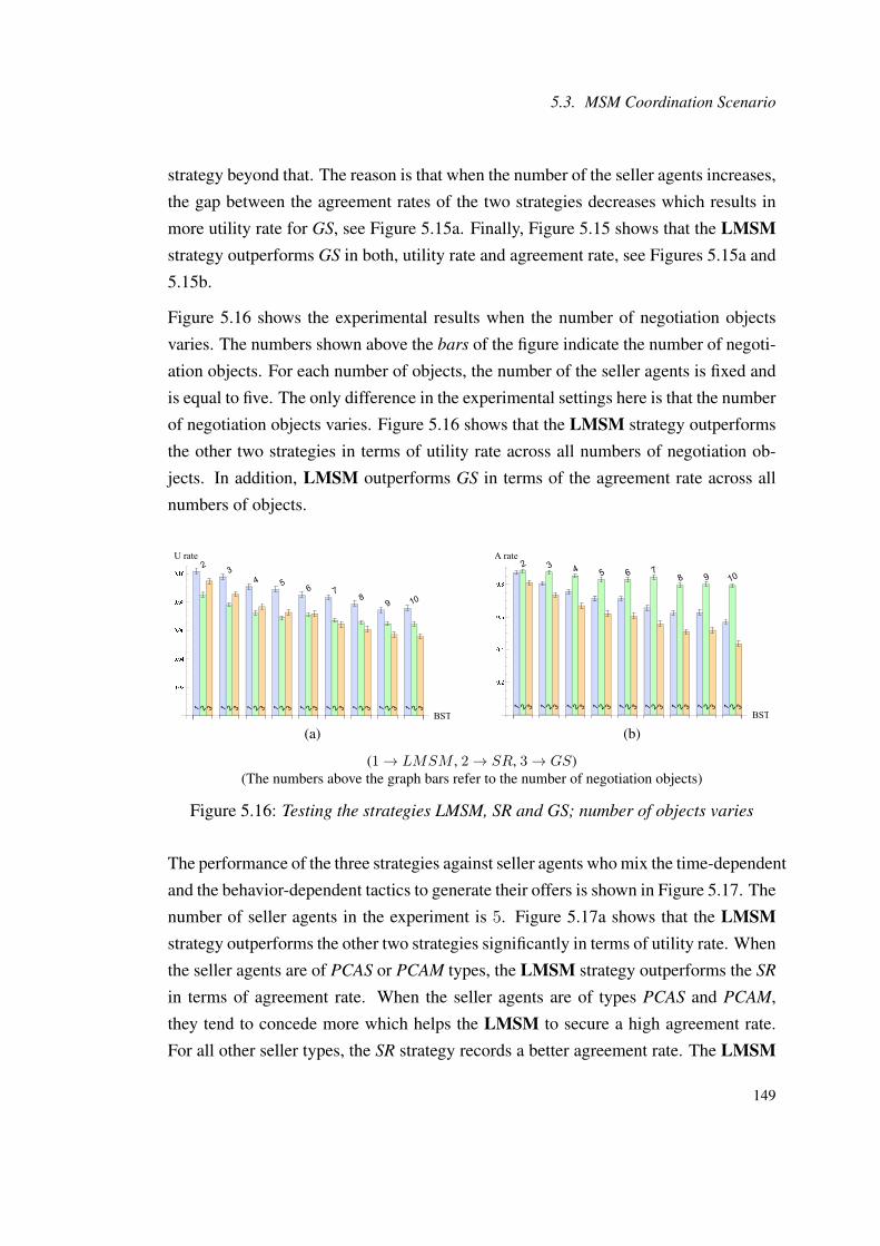
5.3. MSM Coordination Scenario
strategy beyond that. The reason is that when the number of the seller agents increases,
the gap between the agreement rates of the two strategies decreases which results in
more utility rate for GS, see Figure 5.15a. Finally, Figure 5.15 shows that the LMSMstrategy outperforms GS in both, utility rate and agreement rate, see Figures 5.15a and
5.15b.
Figure 5.16 shows the experimental results when the number of negotiation objects
varies. The numbers shown above the bars of the figure indicate the number of negoti-
ation objects. For each number of objects, the number of the seller agents is fixed and
is equal to five. The only difference in the experimental settings here is that the number
of negotiation objects varies. Figure 5.16 shows that the LMSM strategy outperforms
the other two strategies in terms of utility rate across all numbers of negotiation ob-
jects. In addition, LMSM outperforms GS in terms of the agreement rate across all
numbers of objects.
(a) (b)
(1→ LMSM , 2→ SR, 3→ GS)(The numbers above the graph bars refer to the number of negotiation objects)
Figure 5.16: Testing the strategies LMSM, SR and GS; number of objects varies
The performance of the three strategies against seller agents who mix the time-dependent
and the behavior-dependent tactics to generate their offers is shown in Figure 5.17. The
number of seller agents in the experiment is 5. Figure 5.17a shows that the LMSMstrategy outperforms the other two strategies significantly in terms of utility rate. When
the seller agents are of PCAS or PCAM types, the LMSM strategy outperforms the SR
in terms of agreement rate. When the seller agents are of types PCAS and PCAM,
they tend to concede more which helps the LMSM to secure a high agreement rate.
For all other seller types, the SR strategy records a better agreement rate. The LMSM
149
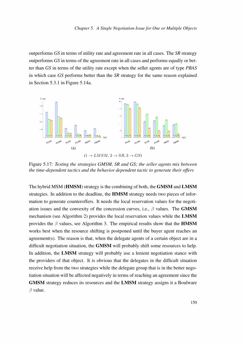
Chapter 5. A Single Negotiation Issue for One or Multiple Objects
outperforms GS in terms of utility rate and agreement rate in all cases. The SR strategy
outperforms GS in terms of the agreement rate in all cases and performs equally or bet-
ter than GS in terms of the utility rate except when the seller agents are of type PBAS
in which case GS performs better than the SR strategy for the same reason explained
in Section 5.3.1 in Figure 5.14a.
(a) (b)
(1→ LMSM , 2→ SR, 3→ GS)
Figure 5.17: Testing the strategies GMSM, SR and GS; the seller agents mix betweenthe time-dependent tactics and the behavior dependent tactic to generate their offers
The hybrid MSM (HMSM) strategy is the combining of both, the GMSM and LMSMstrategies. In addition to the deadline, the HMSM strategy needs two pieces of infor-
mation to generate counteroffers. It needs the local reservation values for the negoti-
ation issues and the convexity of the concession curves, i.e., β values. The GMSMmechanism (see Algorithm 2) provides the local reservation values while the LMSMprovides the β values, see Algorithm 3. The empirical results show that the HMSMworks best when the resource shifting is postponed until the buyer agent reaches an
agreement(s). The reason is that, when the delegate agents of a certain object are in a
difficult negotiation situation, the GMSM will probably shift some resources to help.
In addition, the LMSM strategy will probably use a lenient negotiation stance with
the providers of that object. It is obvious that the delegates in the difficult situation
receive help from the two strategies while the delegate group that is in the better nego-
tiation situation will be affected negatively in terms of reaching an agreement since the
GMSM strategy reduces its resources and the LMSM strategy assigns it a Boulware
β value.
150
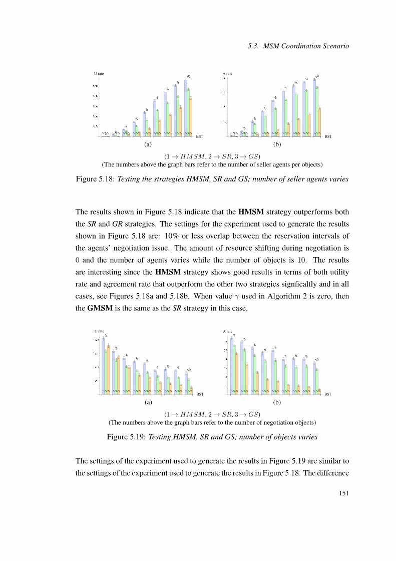
5.3. MSM Coordination Scenario
(a) (b)
(1→ HMSM , 2→ SR, 3→ GS)(The numbers above the graph bars refer to the number of seller agents per objects)
Figure 5.18: Testing the strategies HMSM, SR and GS; number of seller agents varies
The results shown in Figure 5.18 indicate that the HMSM strategy outperforms both
the SR and GR strategies. The settings for the experiment used to generate the results
shown in Figure 5.18 are: 10% or less overlap between the reservation intervals of
the agents’ negotiation issue. The amount of resource shifting during negotiation is
0 and the number of agents varies while the number of objects is 10. The results
are interesting since the HMSM strategy shows good results in terms of both utility
rate and agreement rate that outperform the other two strategies signficaltly and in all
cases, see Figures 5.18a and 5.18b. When value γ used in Algorithm 2 is zero, then
the GMSM is the same as the SR strategy in this case.
(a) (b)
(1→ HMSM , 2→ SR, 3→ GS)(The numbers above the graph bars refer to the number of negotiation objects)
Figure 5.19: Testing HMSM, SR and GS; number of objects varies
The settings of the experiment used to generate the results in Figure 5.19 are similar to
the settings of the experiment used to generate the results in Figure 5.18. The difference
151
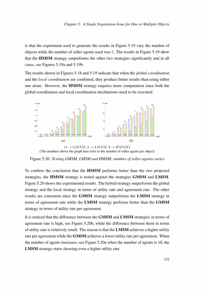
Chapter 5. A Single Negotiation Issue for One or Multiple Objects
is that the experiment used to generate the results in Figure 5.19 vary the number of
objects while the number of seller agents used was 5. The results in Figure 5.19 show
that the HMSM strategy outperforms the other two strategies significantly and in all
cases, see Figures 5.19a and 5.19b.
The results shown in Figures 5.18 and 5.19 indicate that when the global coordination
and the local coordination are combined, they produce better results than using either
one alone. However, the HMSM strategy requires more computation since both the
global coordination and local coordination mechanisms need to be executed.
(a) (b)
(1→ GMSM , 2→ LMSM , 3→ HMSM )(The numbers above the graph bars refer to the number of seller agents per object)
Figure 5.20: Testing GMSM, LMSM and HMSM; number of seller agents varies
To confirm the conclusion that the HMSM performs better than the two proposed
strategies, the HMSM strategy is tested against the strategies GMSM and LMSM.
Figure 5.20 shows the experimental results. The hybrid strategy outperforms the global
strategy and the local strategy in terms of utility rate and agreement rate. The other
results are consistent since the GMSM strategy outperforms the LMSM strategy in
terms of agreement rate while the LMSM strategy performs better than the GMSMstrategy in terms of utility rate per agreement.
It is noticed that the difference between the GMSM and LMSM strategies in terms of
agreement rate is high, see Figure 5.20b, while the difference between them in terms
of utility rate is relatively small. The reason is that the LMSM achieves a higher utility
rate per agreement while the GMSM achieves a lower utility rate per agreement. When
the number of agents increases, see Figure 5.20a when the number of agents is 10, the
LMSM strategy starts showing even a higher utility rate.
152
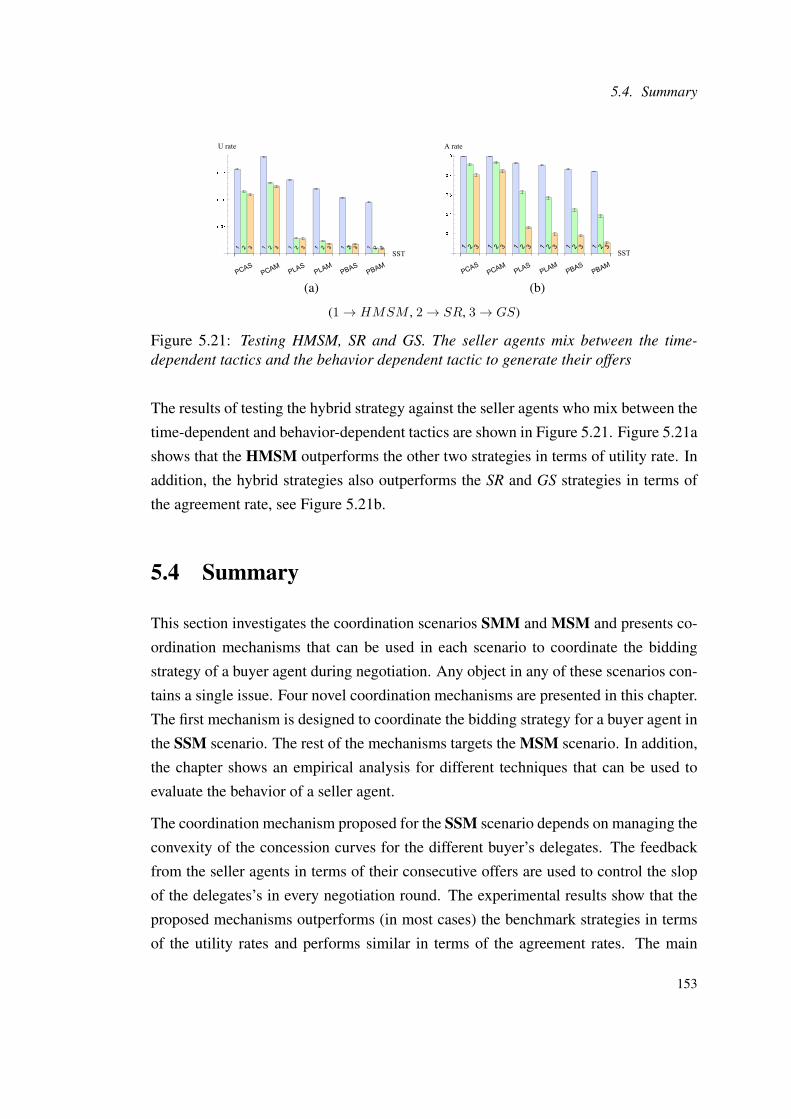
5.4. Summary
(a) (b)
(1→ HMSM , 2→ SR, 3→ GS)
Figure 5.21: Testing HMSM, SR and GS. The seller agents mix between the time-dependent tactics and the behavior dependent tactic to generate their offers
The results of testing the hybrid strategy against the seller agents who mix between the
time-dependent and behavior-dependent tactics are shown in Figure 5.21. Figure 5.21a
shows that the HMSM outperforms the other two strategies in terms of utility rate. In
addition, the hybrid strategies also outperforms the SR and GS strategies in terms of
the agreement rate, see Figure 5.21b.
5.4 Summary
This section investigates the coordination scenarios SMM and MSM and presents co-
ordination mechanisms that can be used in each scenario to coordinate the bidding
strategy of a buyer agent during negotiation. Any object in any of these scenarios con-
tains a single issue. Four novel coordination mechanisms are presented in this chapter.
The first mechanism is designed to coordinate the bidding strategy for a buyer agent in
the SSM scenario. The rest of the mechanisms targets the MSM scenario. In addition,
the chapter shows an empirical analysis for different techniques that can be used to
evaluate the behavior of a seller agent.
The coordination mechanism proposed for the SSM scenario depends on managing the
convexity of the concession curves for the different buyer’s delegates. The feedback
from the seller agents in terms of their consecutive offers are used to control the slop
of the delegates’s in every negotiation round. The experimental results show that the
proposed mechanisms outperforms (in most cases) the benchmark strategies in terms
of the utility rates and performs similar in terms of the agreement rates. The main
153
Chapter 5. A Single Negotiation Issue for One or Multiple Objects
benchmark strategy relies on historical data to determine the value of the next proposal
in every negotiation round.
Since the MSM scenario assumes multiple providers for each agent, two coordination
levels are defined: global coordination and local coordination. The global coordination
mechanism focuses on managing the local reservation values for the objects’ issues.
The global coordination mechanism changes the local reservation values by shifting
resources from one group of delegates to another according to their need. The local
coordination mechanism focuses on a given group of providers and manages the slop of
the concession curve for each group of delegates accordingly. The hybrid mechanism
combines both, the global and local coordination mechanisms. The experimental re-
sults show that the proposed global coordination strategy outperforms the global strat-
egy proposed in the literature in terms of the agreement rates and performs similar or
better in terms of the utility rates. The benchmark strategy reassigns new reservation
values when a certain negotiation is ended. On the other hand, the proposed global
strategy does not wait for a negotiation to finish before reassigning new reservation
values, it rather assigns new reservation values based on the current need of delegates.
The experimental results show that the proposed global strategy performs better than
the local strategy in terms of the agreement rates and vice versa in terms of the utility
rates. On the other hand, the local strategy performs better than the other strategies in
terms of the utility rates. It also outperforms the GS in terms of the agreement rates.
The hybrid strategy outperforms other strategies in terms of the utility and agreement
rates when the amount of resource shifting during negotiation is 0. However, the pro-
posed strategies work best when the overlap percentages between the reservation inter-
vals of issues are small. In other words, the proposed strategies work best under diffi-
cult negotiation environments. The same applies to the benchmark global coordination
strategy. Moreover, the results show that the recent concession measure performs equal
or better than the other measures when evaluating the behaviors of the opponents.
Most of the works in the literature address the single issue negotiation. This chapter
proposes a coordination method that performs better than a state-of-the-art coordina-
tion method. In addition, the state-of-the-art coordination mechanism requires histori-
cal data while the proposed coordination method requires no historical data. Moreover,
this chapter considers negotiations over multiple distinct objects while the work in the
literature rarely considers concurrent negotiations over multiple distinct objects.
154

Chapter 6
A Single Object with MultipleNegotiation Issues
This chapter investigates the single object multiple issues and multiple providers (SMM)
coordination scenario where a buyer agent negotiates with multiple seller agents over
an object characterized by multiple issues. Firstly, a novel offer generation mecha-
nism, the Iterative Offer Generation (IOG), is introduced. The mechanism is used by
the buyer agent to generate counteroffers when it decides to use either a trade-off tac-
tic or a concession tactic. Secondly, a novel one-to-many meta-strategy coordination
mechanism is presented. The meta-strategy is based on the idea of alternating be-
tween a concession tactic and a trade-off tactic during negotiation when generating
counteroffers. The decision to use either tactic depends on the level of cooperation
by the seller agents in terms of their concession in the current negotiation. The ex-
perimental evaluation includes two parts: the meta-strategy evaluation part and the
IOG-concession evaluation part. In addition to the agreement rate and the utility rate
performance criteria, the social welfare and the fairness of the agreements criteria are
also considered.
6.1 Introduction
In real life, people need to consider more than one issue during negotiation. In spite
of the fact that the price is one of the most important issues in business negotiations,

Chapter 6. A Single Object with Multiple Negotiation Issues
other issues such as reliability, delivery time and warranty time are also important.
This chapter extends the previous chapter by considering a more realistic negotiation
scenario where a negotiation object contains multiple issues. The SMM coordination
scenario can represent a case in any of the motivating scenarios presented in Chapter
1. For example, a cloud client might want to negotiate with cloud providers over
a service that has the issues price, size etc., see Section 1.2.1. In the supply chain
domain, a customer can negotiate with multiple suppliers over price, quantity, delivery
time and the quality of some raw material, see Section 1.2.3. Finally, a travel agent can
negotiate price and travel time of a certain journey.
When two agents negotiate over multiple issues, they can follow the sequential pro-
cedure, the simultaneous procedure or the package deal procedure. The sequential
procedure allows agents to negotiate issues in sequence, i.e., one after another. In the
simultaneous procedure, agents negotiate the issues simultaneously but independently
of each other. When agents use the package procedure, each agent proposes a value
for each issue (concurrently) in each negotiation round. The package deal is proven
to be the optimal procedure for each party [40]. Since we are dealing with concurrent
one-to-many negotiation, we assume that a buyer agent proposes a value(s) for each
issue of each object in the same time frame and receives offers from all seller agents
in the next time frame.
This chapter investigates the SMM coordination scenario where a buyer agent is nego-
tiating with multiple seller agents over an object characterized by multiple negotiation
issues, see Figure 6.1. Many possible application domains can be represented by this
form of negotiation, such as the supply chain domain, the task allocation and order
fulfillment problems [157]. For example, a manufacturer needs to procure raw materi-
als and in most cases, more than one supplier exists in the market. One of the possible
approaches for procuring raw materials is to negotiate with multiple potential suppliers
concurrently. In the service oriented domain for example, a client can negotiate with
multiple service providers concurrently over the SLAs for the purpose of procuring
one service or more [100].
The coordination approaches presented in the previous chapter were based either on
managing the convexity curve or managing the local reservation values during negoti-
ation. Since this chapter assumes multiple negotiation issues per object, the proposed
156
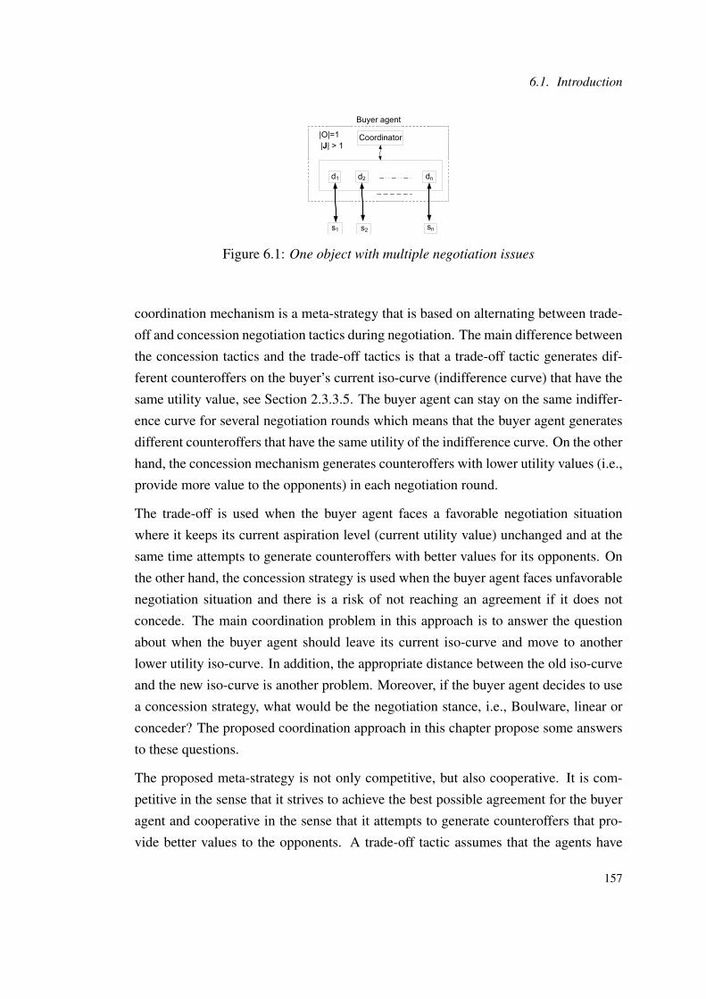
6.1. Introduction
Figure 6.1: One object with multiple negotiation issues
coordination mechanism is a meta-strategy that is based on alternating between trade-
off and concession negotiation tactics during negotiation. The main difference between
the concession tactics and the trade-off tactics is that a trade-off tactic generates dif-
ferent counteroffers on the buyer’s current iso-curve (indifference curve) that have the
same utility value, see Section 2.3.3.5. The buyer agent can stay on the same indiffer-
ence curve for several negotiation rounds which means that the buyer agent generates
different counteroffers that have the same utility of the indifference curve. On the other
hand, the concession mechanism generates counteroffers with lower utility values (i.e.,
provide more value to the opponents) in each negotiation round.
The trade-off is used when the buyer agent faces a favorable negotiation situation
where it keeps its current aspiration level (current utility value) unchanged and at the
same time attempts to generate counteroffers with better values for its opponents. On
the other hand, the concession strategy is used when the buyer agent faces unfavorable
negotiation situation and there is a risk of not reaching an agreement if it does not
concede. The main coordination problem in this approach is to answer the question
about when the buyer agent should leave its current iso-curve and move to another
lower utility iso-curve. In addition, the appropriate distance between the old iso-curve
and the new iso-curve is another problem. Moreover, if the buyer agent decides to use
a concession strategy, what would be the negotiation stance, i.e., Boulware, linear or
conceder? The proposed coordination approach in this chapter propose some answers
to these questions.
The proposed meta-strategy is not only competitive, but also cooperative. It is com-
petitive in the sense that it strives to achieve the best possible agreement for the buyer
agent and cooperative in the sense that it attempts to generate counteroffers that pro-
vide better values to the opponents. A trade-off tactic assumes that the agents have
157
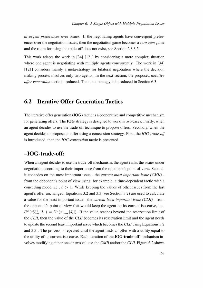
Chapter 6. A Single Object with Multiple Negotiation Issues
divergent preferences over issues. If the negotiating agents have convergent prefer-
ences over the negotiation issues, then the negotiation game becomes a zero-sum game
and the room for using the trade-off does not exist, see Section 2.3.3.5.
This work adapts the work in [34] [121] by considering a more complex situation
where one agent is negotiating with multiple agents concurrently. The work in [34]
[121] considers mainly a meta-strategy for bilateral negotiation where the decision
making process involves only two agents. In the next section, the proposed iterative
offer generation tactic introduced. The meta-strategy is introduced in Section 6.3.
6.2 Iterative Offer Generation Tactics
The iterative offer generation (IOG) tactic is a cooperative and competitive mechanism
for generating offers. The IOG strategy is designed to work in two cases. Firstly, when
an agent decides to use the trade-off technique to propose offers. Secondly, when the
agent decides to propose an offer using a concession strategy. First, the IOG-trade-off
is introduced, then the IOG-concession tactic is presented.
–IOG-trade-off:When an agent decides to use the trade-off mechanism, the agent ranks the issues under
negotiation according to their importance from the opponent’s point of view. Second,
it concedes on the most important issue - the current most important issue (CMII) -
from the opponent’s point of view using, for example, a time-dependent tactic with a
conceding mode, i.e., β > 1. While keeping the values of other issues from the last
agent’s offer unchanged, Equations 3.2 and 3.3 (see Section 3.2) are used to calculate
a value for the least important issue - the current least important issue (CLII) - from
the opponent’s point of view that would keep the agent on its current iso-curve, i.e.,
Ud(xt+1d→s
[Jq]) = Ud(xtd→s
[Jq]). If the value reaches beyond the reservation limit of
the CLII, then the value of the CLII becomes its reservation limit and the agent needs
to update the second least important issue which becomes the CLII using Equations 3.2
and 3.3 . The process is repeated until the agent finds an offer with a utility equal to
the utility of its current iso-curve. Each iteration of the IOG-trade-off mechanism in-
volves modifying either one or two values: the CMII and/or the CLII. Figure 6.2 shows
158

6.2. Iterative Offer Generation Tactics
an illustration to the IOG-trade-off technique. The figure shows eight negotiation is-
sues ordered from the most important issue to the opponent in the far left to the least
important issue to opponent in far right. It also shows the reservation value of each
issue. The utility of the last offer is 0.6 which is the utility of the current iso-curve,
see figure 6.2. In the first iteration, the agent concedes on issue j1 which is the most
important issue from the opponent’s point of view by changing its value from 40 to 50.
This amount of concession changes the utility of the composite offer from 0.6 to 0.5.
In this case, the agent needs to modify the values of some other issue(s) to bring the
utility to 0.6. As the technique specifies, it uses Equations 3.2 and 3.3 to calculate a
new value for issue j8. Assume that the calculated value is 0 that is required to change
the utility of the offer from 0.5 to 0.6, see iteration 2. The problem here is that the
minimum value that can be assigned to issue j8 is 10. The issue j8 is assigned 10 and
the calculated utility become 0.55, see iteration 3. The next step is to move to the
second least important issue (j7) and modifies its value. Assume that Equations 3.2
and 3.3 assign the value 43 to j7 that makes the utility of the offer equals to 0.6. At
this point, the algorithm stops. In case changing the value of issue j7 does not bring
the utility to 0.6, then the algorithm moves to issue j6 etc. Finally, if it is not possible
to concede on issue j1 because the last value of the issue j1 was its reservation value,
then the algorithm concedes on the second most important issue from the opponent’s
point of view which is j2 in our example.
Figure 6.2: Illustration of the IOG-trade-off mechanism
It is assumed that an agent is capable of ranking the issues from its point of view, for
example, an agent is able to say whether money or delivery time is more important.
However, ranking the same issues from the opponent’s point of view is a nontrivial
159

Chapter 6. A Single Object with Multiple Negotiation Issues
task and it is an important research matter, e.g., see [22]. The opponent’s issue ranking
mechanism proposed here works as follows: An agent finds the percentage of the
concession offered on each issue in the previously received two offers, then it ranks the
importance of the issues accordingly. For example, Table 6.1 shows offers exchanged
between two agents in two negotiation rounds for the price and quantity issues. The
percentage of the seller concession on the price is (100 − 10)/100 = 10 % while the
percentage of its concession on the quantity is (11 − 5)/11 = 54.54 %. It can be
detected that the price issue is more important to the seller agent than the quantity
issue, hence the buyer agent can rank the issues according to their importance from the
seller agent’s point of view: price quantity.
Table 6.1: Example of exchanged offers over two negotiation issues
Price Quantityround 1 seller 100 5
buyer 10 50round 2 seller 90 11
buyer 30 48
An agent using the explained ranking method repeats the ranking process at the start of
each negotiation round since the assumption is that the opponent may change its men-
tal state and hence the importance of different issues may change during negotiation.
This ranking method is flexible since an agent can detect changes in its opponent’s
mental state by tracking the percentages of concessions offered on each issue in each
negotiation round. However, in many cases, an agent would have some experience or
domain knowledge that enables it from guessing the rank of negotiation issues from
its opponent’s point of view especially when the negotiating agents are of buyer and
seller types. As the issue ranking is not in the scope of this thesis, in the experimental
work, a buyer agent is assumed to have partial knowledge about the importance of the
issues from the sellers’ point of view.
As previously stated, one of the two important conditions that are necessary to apply
the trade-off mechanism effectively is that agents have divergent preferences over at
least one issue (see Section 2.3.3.5). It is obvious from Table 6.1 that the seller agent
is more sensitive towards the price when compared to the buyer agent, while the buyer
agent is more sensitive to the quantity when compared to the seller agent. In this
case, both agents have divergent preferences over the two issues and the buyer agent
160

6.2. Iterative Offer Generation Tactics
concedes more on the price (while staying on its indifference curve) while the seller
agent concedes more on the quantity issue while staying on its current indifference
curve assuming that both agents use the IOG-trade-off mechanism.
A second numerical example that represents a seller agent (∀ji ∈ J, IVji > RVji) uses
Equations 3.2 and 3.3 to find the next offer is given next. Assume J = j1, j2, j3 and
the reservation intervals for the issues are j1 ∈ [10, 30], j2 ∈ [20, 40], j3 ∈ [15, 35].
Assume that the issues are ranked as follows:j2 j1 j3 and the last proposed
composite offer was j1 = 20, j2 = 30, j3 = 25. Let the utility of the current indif-
ference curve be equal to 0.6 and the weight vector W = 0.5, 0.3, 0.2. According
to the IOG-trade-off, an agent concedes first on the most important issue which is
j2. Assume that the agent decides to offer 22 on the issue j2 using a time-dependent
tactic with a conceder mode. Now, the value of j1 is kept as is for the current it-
eration and the objective is to find a value for the issue j3 using the equations 3.2
and 3.3 as follows. First, the uj3 needs to be found from equation 3.3 where 0.6 =
0.5∗((30−20)/(30−10))+0.3∗((40−22)/(40−20))+0.2∗uj3 . Solving the equation
results in uj3 = 0.4. The next step is the find the value of j3 that produces the utility
0.4 from equation 3.2 as follows: 0.4 = (35−xj3)/(35−15), solving for xj3 , xj3 = 27
which means that the next composite offer will be j1 = 20, j2 = 22, j3 = 27.
The above example required only one step since the value of the issue j3 that is needed
to keep the current indifference curve utility (i.e., 0.6) did not go beyond the reserva-
tion value of the issue j3. If the required value of the issue j3 to keep the current utility
level is, e.g., 37, then the value of the issue j3 is assigned 35 which is its reservation
value and the next iteration of the algorithm proceeds to find a new value for the issue
j1 (the current least important issue) that keeps the current utility unchanged. If this
step is also unsuccessful, then the value j2 = 22 needs to be changed, i.e., a higher
value needs to be proposed to keep the current utility of the indifference curve.
–IOG-concession:The IOG-concession is a concession offer generation method where an agent needs
first to decide its current acceptable utility value that is less than its previous one. The
next step is to find a value for each issue in the composite offer to be proposed next.
The agent starts conceding on the CMII from the opponent’s point of view. The process
here is similar to the process of computing the value of a composite offer in case the
161

Chapter 6. A Single Object with Multiple Negotiation Issues
agent uses the IOG-trade-off mechanism. The difference here is that the utility of the
current composite offer is lower than the utility of the previous composite offer.
It is true that an agent cares about the weighted average utility (when negotiation is-
sues are linearly dependent) which means that the agent may concede on any issue
that brings its utility to the designated utility level and the issues can be selected ran-
domly since the utility of the composite offer is the important criterion here. However,
adopting the IOG-concession mechanism has two benefits:
• In case agents have divergent preferences over issues, the IOG-concession mech-
anism can result in a better offer value for the opponent which may improve the
chance of reaching an agreement quickly. In addition to saving time by reach-
ing an agreement quickly, if an agreement is reached in the current negotiation
round, the conceding agent does not lose more utility if negotiation continues.
It can happen that the conceding agent may need to concede again in the next
negotiation round.
• The IOG-concession mechanism may improve social welfare when the propos-
ing agent provides more concessions on the issues that are more important for
the opponents first.
One way to determine the required aspiration level at any time during negotiation is to
use Equation 6.1 that depends on both, the time elapsed and the β value. If an agent is
in desperate need for an agreement, it uses large β values which means that the agent
is willing to accept low utility offers in exchange for reaching an agreement. The value
of β can cause a conceder, a Boulware or a linear behavior which is similar to the role
of β in the time-dependent tactics.
Ud(xtd→s
[Jq]) = 1− (t/tdmax)(1/β) (6.1)
In Equation 6.1, t is the current time, tdmax is the agent’s deadline. For example, at time
t = 0, the results of the equation (t/tdmax)(1/β) equals 0, then the required aspiration
level equals 1. That is normal since an agent at the start of negotiation starts with high
aspiration level, then it concedes by reducing its aspiration level during negotiation.
In one-to-many negotiations, other factors can be used to determine the current re-
quired utility value such as the number of negotiation instances. More negotiation
162

6.3. The Meta-Strategy Model
instances means more opponents and hence better bargaining power for the agent on
the ‘one’ side. In other cases, an agent chooses a fixed amount of concession in each
negotiation round. For example, an agent may concede 0.05 in each time it decides to
use a concession offering mechanism.
6.3 The Meta-Strategy Model
The proposed negotiation meta-strategy is a strategy that selects a certain offer genera-
tion technique from a predefined set of offer generation techniques during negotiation.
The selection criteria depends on the current negotiation situation in terms of the num-
ber and the behaviors of the current opponents. As mentioned in the solution approach,
see Section 4.3, the buyer agent may change its negotiation strategy by changing any
of its strategy components or their associated parameters. This chapter considers the
Θ strategy component which is the set of offer generation techniques and their asso-
ciated parameters. In particular, the proposed meta-strategy may use a different offer
generation mechanism in each negotiation round.
As mentioned in the introduction of this chapter, the buyer agent alternates between
a concession tactic and a trade-off tactic during negotiation. The buyer agent uses
the trade-off tactic whenever the situation is favorable, otherwise the buyer uses a
concession tactic. Deciding whether the buyer agent is in a favorable situation depends
on both, the number of opponents and their behaviors in terms of their concessions. If
the opponents are offering generous concessions then the situation is favorable for the
buyer agent, otherwise it is not. More opponents means the buyer agent has more
bargaining power and hence the situation is favorable.
Algorithm 4 summarizes the meta SMM strategy (MSMM). The data preparation steps
are similar to the data preparation presented in Chapter 4. The data preparation is
shown in lines 1− 7.
When considering the situation where the buyer agent has the privilege to renege from
a temporary agreement without paying a penalty, the approach works as follows: in
the first few negotiation rounds, the buyer agent classifies the seller agents into two
groups, a favorable group and unfavorable group depending on their relative behavior
(relative to the buyer’s behavior) by comparing the amount of concessions offered by
163

Chapter 6. A Single Object with Multiple Negotiation Issues
each delegate di and its opponent si. The buyer agent uses the meta-strategy with the
favorable group, while using the concession strategy with the unfavorable group.
At this point, we have a few problems to deal with. The first one is how an opponent’s
behavior is measured? The second one is how much the buyer agent concedes when it
chooses to use the concession strategy? A third one is how the distance between two
indifference curves is determined when the buyer agent moves from one indifference
curve to another during negotiation where the distance is measured in terms of utility.
Algorithm 4 (MMSM)Require: < Xt−1
d1,1↔s1,1[j], Xt−1
d1,2↔s1,2[j], ..., Xt−1
d1,n1↔s1,n1
[j] >, ...,
< Xt−1dm,1↔sm,1
[j], Xt−1dm,2↔sm,2
[j], ..., Xt−1dm,mn↔sm,mn
[j] >
1: for i = 1→ n do . see Section 4.3, n is the number of seller agents2: Fi = Usi − Udi3: end for4: ∆F = < F1, F2, ..., Fn >
5: for all (Fi ∈ ∆F ) do6: if (Fi > 0) then7: add(fs, si)
8: else9: add(fs
′, si)
10: end if11: end for12: if (fs 6= ∅) then13: NegoTatcic = trade-off
14: end if15: if (fs
′ 6= ∅) then16: NegoTatcic = time-dependent
17: end if18: if (fs 6= ∅ and fs′ == ∅) then19: set = sort(fs)
20: fs′
= take(set, 1, |set|/2) . integer division21: fs = take(set, |set|/2 + 1, |set|)22: end if23: if (fs == ∅ and fs′ 6= ∅) then24: set = sort(fs)
25: fs′
= take(set, 1, |set|/2) . integer division26: fs = take(set, |set|/2 + 1, |set|)27: end if28: end algorithm
164
6.3. The Meta-Strategy Model
In this chapter, the utility difference between consecutive offers is considered instead
of considering the difference in concessions for the purpose of evaluating the oppo-
nents. The reason is that the negotiation object is characterized by several issues and
it is difficult to consider the difference in concession between each pair of issues since
evaluating the behavior of an opponent becomes more difficult given that agents may
have different priorities over the negotiation issues. The utility difference evaluates the
opponent agents and works equally as well as the concession difference. The process
of using the utility difference is shown in lines 1-3 in Algorithm 4. In the algorithm,
Usi stands for the difference in utility between the last two offers proposed by the seller
agent si whereas Udi stands for the difference between the last two counteroffers pro-
posed by the delegate di. Lines 5-11 classify the current seller agents into either a
favorable set (fs) or unfavorable set (fs′) depending on the results in the utility differ-
ence shown in lines 1-3. If the difference in utility between the last two counteroffers
of a delegate di is more than the difference in utility between the two offers of seller
agent si (Fi in Algorithm 4) then the seller agent si is added to the favorable group
fs, otherwise it is added to the unfavorable group fs′ . The classification process is
performed at the start of negotiation. The buyer agent chooses to use a trade-off tactic
with the fs group and a concession tactic with the fs′ group.
It can happen that all the seller agents are classified in the set fs. In this case, if the
buyer agent chooses to use a trade-off tactic, it might jeopardize reaching an agreement.
To reduce the risk of not reaching an agreement, lines 18-20 sort the fs set ascendingly
and take the first half of the seller agents and assign it to a new fs′ set and assign the
second half (the more favorable seller agents) to a new fs set. The algorithm uses the
meta-strategy with the new fs set and the concession strategy with the new fs′ set.
If all seller agents are assigned to the fs′ set, then a similar procedure is applied to
ensure that the buyer agent does not use only a concession tactic with all seller agents,
see lines 23-26.
When the buyer agent uses a trade-off negotiation tactic, it needs to decide when to
move from one iso-curve to another during negotiation, since if it stays on the same
iso-curve for a long time, it might jeopardize reaching an agreement. The reason is that
the buyer agent could reach a point where it is difficult to propose new counteroffers
to the seller agents that have extra value for them. It means that the buyer agent is
not willing to concede anymore from the sellers’ point of view which might end the
165
Chapter 6. A Single Object with Multiple Negotiation Issues
negotiation with a conflict outcome. On the other hand, since agents are negotiating
under incomplete knowledge, the buyer agent cannot tell when its current proposal
does not provide any added value to its opponent than the previous one. However,
since the buyer agent is negotiating with multiple seller agents, it can use the behaviors
of the seller agents with whom it uses the trade-off tactic to decide when to move from
one iso-curve to another. Deciding when to move from the current iso-curve to a new
iso-curve with lower utility is considered next.
The buyer agent needs to define a deadlock point where it should move to a new iso-
curve in the next negotiation round. There could be many signs for a deadlock point.
For example, if the seller agents start offering proposals with lower utility than the
previous ones, then this could be a sign for a deadlock. Since the seller agents in this
thesis are assumed to offer equal or more utility proposal values than the previously
offered ones, a different deadlock indicator needs to be considered. As a proposed so-
lution, the buyer agent finds the first-order utility difference (Su) from the last received
two offers by each member in the set fs and the first-order utility difference (Bu) from
the last two counteroffers proposed by their counterpart delegates. The buyer agent
subtracts Bu from Su, i.e., udiff = Su − Bu. If the maximum number in the set udiffis less than or equal to 0, then the buyer agent reaches a deadlock point and needs to
move to a new iso-curve. It means that none of the seller agents in the set fs offers
more concession than the concession offered by its counterpart delegate in the last two
negotiation rounds which is considered unfavorable situation for the buyer agent.
When the buyer agent using the MSMM strategy decides to move to a new iso-curve
at time t, the distance between the old iso-curve and the new iso-curve is based on the
smallest first-order difference in the utility offered by any seller agent in fs in the last
two negotiation rounds. In other words, the buyer agent reduces its aspiration level by
the amount of the least utility difference offered by any seller agent in fs. The intuition
behind this decision is to imitate the concession of the most difficult opponent in fs
that improves the chance of reaching a valuable agreement for the buyer agent. Other
work in the literature [36] assumes a fixed distance between iso-curves. However, this
is a strong assumption since other factors need to be considered such as time, behaviors
of the opponents, etc.
166

6.4. Experimental Evaluation
6.4 Experimental Evaluation
This section shows the experimental results for testing both, the MSMM strategy and
the IOG-concession tactic. All the results are analyzed and discussed.
6.4.1 Experimental Settings
The buyer agent uses the time dependent-tactic to generate its first two counteroffers
then it uses either the MSMM strategy or the IOG-concession tactic to generate the
rest of the counteroffers. The MSMM strategy is tested against two buyer agents who
use different negotiation strategies to generate their counteroffers. Since the results
presented in Chapter 5 show that the eCN strategy proposed in [106] outperforms most
of the strategies in the literature, it is selected as a benchmark strategy. In addition, as a
base benchmark strategy, the general negotiation strategy (GS) is also used. The GS is
a strategy where the buyer agent does not change any of its negotiation variables during
negotiation and it can be either a patient strategy or a desperate strategy. As explained
in Chapter 5, the desperate strategy accepts the first acceptable agreement and quits
negotiation while the patient strategy keeps negotiating until it reaches its deadline or
all the seller agents quit negotiation. The general strategy used in this section uses
the patient technique since all the buyer agents are assumed to keep negotiating with
their opponents until they reach their deadlines or all the opponents quit negotiation.
When one of the these two conditions hold, each buyer agent selects agreement with
the highest utility. Since the IOG-concession tactic is a concession tactic, it is tested
against GS which is considered a concession tactic too.
In all the experiments of this chapter, when an agent decides to accept an offer, it first
checks for the utility of the received offer, if it is equal to its current aspiration level
or more, then the agent checks whether each value of each issue in the received offer
is more/less than its reservation value. If the answer is yes, then the offer is accepted,
otherwise the offer is rejected. Moreover, the experiments used to generate the re-
sults in this chapter assume that the buyer agents and the seller agents have divergent
preferences over the negotiation issues.
The following points highlights the general experimental settings:
167

Chapter 6. A Single Object with Multiple Negotiation Issues
• Deadlines. If the system does not require a fixed negotiation time for all agents,
a deadline is randomly selected from the interval [5, 30] at the start of each ne-
gotiation instance for all seller agents. To study the performance of different
negotiation strategies under different deadlines. Experiments are designed to
test the performance of the different buyer strategies when the buyer agents have
both, shorter and longer deadlines than the seller agents’ deadlines. In all exper-
iments, the buyer agents have the same deadline that is selected randomly from
a chosen interval. In addition, the buyer strategies are also tested when all agents
(buyers and sellers) have equal deadlines.
• Agent types. An agent can be either time-dependent, behavior-dependent or
mixed type. The mixed type agent means that the agent mixes between the time-
dependent and the behavior-dependent tactics when generating its offers. Since
the benchmark eCN agent relies only on changing the convexity curve during
negotiation to generate its counteroffers, both eCN and GS buyer agents use
the time-dependent tactics to generate their counteroffers. At the start of each
negotiation instance, all buyer agents are assigned the same β value selected
randomly from the interval [0.1, 5]. At the start of each negotiation instance,
each seller agent selects a β value randomly from the same interval. In addition,
an experiment is designed to test the buyer strategies when the seller agents use
a mixed offer generation strategy.
• Length of the agreement zone. The performance of different strategies are
tested for different lengths of agreement zones, i.e., different percentages of
overlaps between the reservation intervals of negotiation issues of buyer agents
and seller agents, see Section 4.5.2.
• Number of agents and number of issues. The proposed MSMM and IOG-concession strategies is tested with different number of seller agents and with
different number of negotiation issues per object. To test how different buyer
strategies are affected by the different number of seller agents, the experiment
starts with 2 seller agents then 3, 4, ..., 10 agents. While the number of seller
agents are changed, the number of issues is fixed. On the other hand, to test the
strategies against different number of issues, the experiment again starts with 2
issues then 3, 4, ..., 10 issues per object. While changing the number of issues,
the number of seller agents is fixed.
168
6.4. Experimental Evaluation
6.4.2 Experimental Results and Discussion
This section shows the results of the experiments and discusses the results. First, the
performance of the MSMM strategy is tested when the buyers’ deadline is smaller,
larger or equal to the seller agents’ deadlines. Second, the strategy is also tested when
the length of agreement zones between the buyer agents and the seller agents are small
and large. In addition, the MSMM strategy is tested against seller agents who mix
between the time-dependent tactics and the behavior-dependent tactics to generate their
offers. On the other hand, the IOG-concession tactic is tested when all agents select
random deadlines from the same interval and when all agents have equal deadlines.
In the experiments, four evaluation criteria are considered: utility rate, agreement rate,
Nash product rate and utility difference rate. Nash product rate is used as a perfor-
mance criterion for the social welfare [104]. Large Nash product rate indicates better
social welfare. The utility difference rate is the absolute difference between the agree-
ment utility of a seller agent and its counterpart delegate. The utility difference rate
indicates the fairness of the agreements, the lowest utility difference rate the better.
As a reminder of the notation used in the figures of this section, the BST label of the x-
axis stands for the buyer strategies. Each y-axis label refers to a different performance
criteria: U rate is the utility rate, A rate is the agreement rate. Nash prod. is the Nash
product and the U diff. stands for the utility difference. The utility rates, the Nash
product rates and the utility difference rates shown in the figures of this chapter are
calculated per number of the agreements achieved.
In all the experimental results shown in this chapter, when the number of agents per
object varies, the number of issues per object is set to 5 and when the number of
issues per object varies, the number of seller agents per object is set to 5 too. For each
different number of seller agents per object or different number of issues per object, the
experiment is repeated 1000 negotiation rounds. The results are averaged and plotted.
6.4.2.1 Testing under Different Deadline Lengths
The specific experimental settings for testing the MSMM strategy when the buyer
agents have shorter deadlines, longer deadlines and equal deadlines to the seller agents’
deadlines are presented in Table 6.2.
169

Chapter 6. A Single Object with Multiple Negotiation Issues
Table 6.2: Experimental settings of different deadline lengths
Agents or issues per object Deadline descriptionBuyers’
deadlinessellers’
deadlinesBuyers’
beta valuesellers’
beta values OverlapFigurename
Number of agents variesBuyers have
shorter deadlines [5-30] [31-50] [0.5-5] [0.5-10] [0%-100%] 6.3,6.4
Number of issues variesBuyers have
shorter deadlines [5-30] [31-50] [0.5-5] [0.5-10] [0%-100%] 6.5
Number of agents variesBuyers have
longer deadlines [31-50] [5-30] [0.5-5] [0.5-10] [0%-100%] 6.6
Number of issues variesBuyers have
longer deadlines [31-50] [5-30] [0.5-5] [0.5-10] [0%-100%] 6.7
Number of agents variesAll agents haveequal deadlines - - [0.5-5] [0.5-10] [0%-100%] 6.8
Number of issues variesAll agents haveequal deadlines - - [0.5-5] [0.5-10] [0%-100%] 6.9
The overlap in Table 6.2 refers to overlap between the reservation intervals of the ne-
gotiation issues. The columns in Table 6.2 starting from “Buyer’s deadlines” to “Over-
lap” show intervals where a random number from each interval is selected randomly to
specify a certain negotiation parameter for each agent at the start of every negotiation
round. All buyer agents are assigned the same deadline and the same β value at the
start of every negotiation round. Random overlap percentages are selected from the
interval [0%− 100%] for each issue where the seller agents can have different overlap
percentages for the same issue. In addition, a deadline value and a β value are selected
randomly from the intervals shown in Table 6.2 for each seller agent at the start of
every negotiation round. For example in a certain negotiation round, seller agent 1 can
have 20 as a deadline value while seller agent 2 can have 25 as a deadline value etc.
The same applies for the other parameter values. This is to ensure that the seller are
different while the buyer agents are the same except for the bidding strategy they use.
The experimental results when the buyer agents have shorter deadlines than their oppo-
nents’ deadlines are shown in Figure 6.3. When the buyer agents have shorter deadline
lengths, they reach their reservation values before the seller agents do and the same
applies for the seller agents.
The results in Figure 6.3 show that the MSMM strategy outperforms the eCN and
GS strategies in terms of utility rates, see Figure 6.3a. The three buyer agents have no
problem in terms of the agreement rate as shown in Figure 6.3b except that the MSMMstrategy has lower agreement rates than the other two strategies when the number of
seller agents is small≤ 3. Consider the number of seller agents per object is small, e.g.,
2, the classification process in the MSMM strategy then assigns one seller agent to fs
170

6.4. Experimental Evaluation
(a) (b)
(c) (d)(1→MSMM , 2→ eCN , 3→ GS)
(The numbers above the graph bars refer to the number of seller agents per object)
Figure 6.3: The buyer agents have shorter deadlines than the seller agents’ deadlinesand the number of seller agents per object varies.
and another to fs′ . The classification process may change the positions of the seller
agents in the next negotiation round and since the buyer agent has lower deadline than
its opponents’ deadlines, it may have not enough time to adapt to the situation after
the new classification and consequently miss the agreement. The reason behind the
fact that the buyer agents do not have a problem in reaching near 100% agreement rate
in the given settings is that the buyer agents offer their reservation values before the
seller agents do. In addition, there are multiple providers and the chance of reaching
an agreement with at least one of them is high given the fact that agreement zones
between the buyer agents and the seller agents do exist.
The Nash product rates of the MSMM strategy is higher than the Nash product rates
of the other benchmark strategies, see Figure 6.3c. Because the MSMM strategy is
both competitive and cooperative, see Section 6.2. When the number of seller agents
per object increases, the Nash product rate increases for all strategies. The reason
is that the buyer agents achieve higher utility per agreement when the number of the
171

Chapter 6. A Single Object with Multiple Negotiation Issues
sellers is high which increases the Nash product rates. The eCN strategy has the lowest
Nash product rates since it is a very competitive strategy and does not cooperate with
its opponents. The Nash product rates for GS is always higher than the Nash product
rates of the eCN strategy because GS offers more proposal values to its opponents
which increases the Nash product agreement value. When the number of seller agents
per object is high enough (> 10), GS approaches the MSMM in terms if Nash product
rates, see Figure 6.3c. The reason is that when the number of the sellers increases,
the buyer agent using GS has the opportunity to select a more valuable agreement. In
addition, GS offers proposals that have better utility values to its opponents in every
negotiation round. This results in improved Nash product rates.
The utility difference is shown in Figure 6.3d. The utility difference indicates the fair-
ness of an agreement. If the utility difference between two agreement utilities is 0, it
means that each opponent achieves the same utility from the agreement. If the utility
difference for a strategy is lower than the utility difference for another, then the first
strategy achieves an agreement that is more fair than the agreement archived by the
second strategy. In all cases shown in Figure 6.3d, GS has lower utility difference rates
than the other two strategies. The utility difference rates of the MSMM strategy is
higher than the utility difference rates of the eCN and GS strategies. Figure 6.3d shows
that the difference in utility difference between the eCN strategy and MSMM strate-
gies is relatively small when the number of seller agents per object is small. When the
number of seller agents becomes large, the MSMM strategy becomes more competi-
tive and secures high utility agreement when compared to the utility agreement of its
opponent.
The GS achieves the best results in terms of utility difference because GS is a conces-
sion strategy that keeps offering concessions throughout negotiation until it reaches an
agreement. In addition, the seller agents in this experimental settings use a conces-
sion strategy which makes them keep offering concessions throughout negotiation too.
Therefore, the buyer agent using GS and the seller agents using their own concession
strategy keep approaching one another in the offers/counteroffers they propose which
reduces the difference between the buyer’s utility agreement and the seller’s utility
agreement.
In all the experimental results shown for the strategy MSMM, the seller agents’ classi-
172

6.4. Experimental Evaluation
(a) (b)
(c) (d)(1→MSMM , 2→ eCN , 3→ GS)
(The numbers above the graph bars refer to the number of seller agents per object)
Figure 6.4: The buyer agents have shorter deadlines than the seller agents’ deadlinesand the number of seller agents per object varies.
fication process is repeated at the start of each negotiation round except for the results
shown in Figure 6.4. The results in Figure 6.4 show the results under the same experi-
mental settings used for the experiments of Figure 6.3 except that the MSMM strategy
classifies the seller agents at the start of the negotiation instance and do not update the
classification later. The difference between the two classification schemes in terms of
the utility rates is obvious, see Figures 6.3a and 6.4a. When the buyer agent reclassifies
the seller agents at the start of each negotiation round, it gains recent knowledge about
the new objectives and behaviors of the seller agents. In case the buyer agent classifies
the seller agents once at the start of negotiation, the knowledge it gains becomes old
and less effective as the negotiation process continues. Both classification schemes
achieve similar results in terms of the agreement rates, see Figure 6.4b. However, the
classification of the seller agents once at the start of negotiation results in better Nash
product rates and better utility difference rates, see Figures 6.4c and 6.4d. The utility
difference rates are similar to the utility difference rates produced by GS in most cases.
173

Chapter 6. A Single Object with Multiple Negotiation Issues
When the buyer agent seeks to secure high utility results, it needs to classify the seller
agents at the start of every negotiation round. While if the buyer agent cares more
about the social welfare and the fairness of the agreements, it should classify the seller
agents once at the start of negotiation only. This conclusion applies when the seller
agents use the time-dependent tactics to generate their offers. In all the following ex-
perimental results regarding the MSMM strategy, the buyer agent classifies the seller
agents at the start of every negotiation round.
(a) (b)
(c) (d)(1→MSMM , 2→ eCN , 3→ GS)
(The numbers above the graph bars refer to the number of issues per object)
Figure 6.5: The buyer agents have shorter deadlines than the seller agents’ deadlinesand the number of issues per object varies.
The results when the buyer agents have shorter deadlines than the seller agents’ dead-
lines and the number of issues per object varies are shown in Figure 6.5. The numbers
on the top of the figure indicate the number of issues per object. The numbers start with
2 issues per object and increases gradually until 10 issues per object. For the specific
experimental settings, see Table 6.2. As the number of issues per object increases, all
strategies achieve gradually lower utility rates since the agents need to wait and keep
174
6.4. Experimental Evaluation
conceding until they achieve the required utility for the object. However, Figure 6.5a
shows that the MSMM strategy outperforms the other two strategies in terms of utility
rate under all different number of issues per object. As before, the buyer agents have
no problem in reaching agreements under the specified settings, see Figure 6.5b.
The Nash product results are shown in Figure 6.5c. When the number of issues per
object is 2, the MSMS achieves lower Nash product rate than GS and similar to the
eCN strategy. However, as the number of issues per object increases, the MSMMstrategy outperforms the other two strategies. The reason is that when the number of
issues increases, the MSMM strategy starts offering more utility values to its oppo-
nents since the MSMM strategy considers that agents have divergent preferences over
issues when generating its counteroffers. The eCN strategy has the lowest Nash prod-
uct rates. Figure 6.5d shows the utility difference results. The GS performs the best
in terms of utility difference for the same reasons stated earlier. When the number of
issues per object becomes large enough (> 7), the MSMM strategy performs similar
or better than the eCN strategy since it starts offering its opponents more utility values
that reduces the absolute difference between their utility agreements.
The experimental results when the buyer agents have longer deadlines than their oppo-
nents’ deadlines are shown in Figure 6.6. Figure 6.6 shows the results when the number
of seller agents per object varies. Since the seller agents have shorter deadlines, the
seller agents approaches their reservation values before the buyer agents do. Accord-
ingly, the difference in the utility rates between different strategies are not expected to
be large, see Figure 6.6a. However, the MSMM strategy outperforms the other two
strategies in all cases. Since the deadlines for the seller agents are shorter than the
buyers’ deadline, the seller agents offer their reservation values and quit negotiation
before the buyer agents do. That can affect the agreement rates negatively, see Figure
6.6b. However, the MSMM strategy produces equal or better agreement rates than the
other two strategies. When the number of seller agents per object is small, the eCN
strategy performs the worst. The Nash product results show that the MSMM strategy
outperforms the other two strategies in all cases as well, see Figure 6.6c. The eCN
strategy produced the lowest Nash product rates because it is a competitive strategy
that does not show any cooperation with its opponents.
The utility difference results presented in Figure 6.6d show that GS performs the best.
175

Chapter 6. A Single Object with Multiple Negotiation Issues
(a) (b)
(c) (d)(1→MSMM , 2→ eCN , 3→ GS)
(The numbers above the graph bars refer to the number of seller agents per object)
Figure 6.6: The buyer agents have longer deadlines than the seller agents’ deadlinesand the number of seller agents per object varies.
In spite of the MSMM strategy outperforms the eCN strategy in terms of the utility
rates, in many cases, there is no significant difference between the MSMM and eCN
strategies in terms of the utility difference for the reasons stated earlier.
Figure 6.7 shows the experimental results when the buyer agents have longer deadlines
than the seller agents’ deadlines and the number of issues per object varies. As shown
before, when the number of issues per object increases, the general trend is that the
utility rates decreases for all strategies, see Figure 6.7. However, the MSMM strategy
outperforms the benchmark strategies in all cases, see Figure 6.7a. The results of
the agreement rates shown in Figure 6.7b are similar to the agreement rates shown in
Figure 6.6b except for the eCN strategy where its agreement rates decreases when the
number of issues per object increases. To a less extent, the same happens with GS
while the MSMM strategy shows stability in the agreement rates.
The MSMM strategy outperforms the other two strategies in terms of Nash product
176

6.4. Experimental Evaluation
(a) (b)
(c) (d)(1→MSMM , 2→ eCN , 3→ GS)
(The numbers above the graph bars refer to the number of issues per object)
Figure 6.7: The buyer agents have longer deadlines than the seller agents’ deadlinesand the number of issues per object varies.
rates, see Figure 6.7c. In addition, in many cases it performs similar to the eCN strategy
in terms of the utility difference, see Figure 6.7d.
The last set of the experiments in this section is when all agents have equal deadlines.
Starting with the results presented in Figure 6.8 where the number of seller agents
per object varies, Figure 6.8a shows that the MSMM strategy performs better than
the other two strategies and the eCN strategy comes next. Since all agents have equal
deadlines, all buyer agents achieve 100% agreement rates, see Figure 6.8b.
When the number of seller agents per object is small, the MSMM strategy performs
the best in terms of Nash product rates, see Figure 6.8c. When the number of seller
agents per object increases, the MSMM strategy starts producing lower Nash product
rates than the Nash product rates produced by GS. The reason is that when the number
of seller agents per object increases, the MSMM strategy becomes more competitive
and the result is lower Nash product rates. However, The MSMM produces better
177

Chapter 6. A Single Object with Multiple Negotiation Issues
(a) (b)
(c) (d)(1→MSMM , 2→ eCN , 3→ GS)
(The numbers above the graph bars refer to the number of seller agents per object)
Figure 6.8: All agents have the same deadline and the number of seller agents perobject varies.
Nash product rates than the ones produced by the eCN strategy in all cases shown in
Figure 6.8c.
The utility difference rates show that the MSMM strategy outperforms the eCN strat-
egy when the number of seller agents per object is small, see Figure 6.8d. However,
when the number of sellers per object increases, the MSMM strategy performs the
worst since it becomes more competitive in the given settings. The GS performs the
best in terms of the utility difference rates for the same reasons stated earlier.
Figure 6.9 shows the experimental results when the number of issues per object varies.
The utility rates show the same trend as before, see Figure 6.9a. The MSMM strategy
is also consistent to outperform the benchmark strategies. The results for the agree-
ment rates are as in Figure 6.8b where all buyer agents achieve 100% agreement rates
because all agents have equal deadlines and the agreement zones between the buyers
and sellers exist, see Figure 6.9b.
178
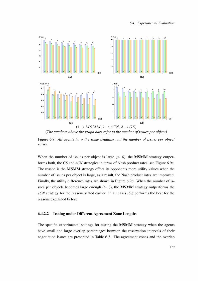
6.4. Experimental Evaluation
(a) (b)
(c) (d)(1→MSMM , 2→ eCN , 3→ GS)
(The numbers above the graph bars refer to the number of issues per object)
Figure 6.9: All agents have the same deadline and the number of issues per objectvaries.
When the number of issues per object is large (> 6), the MSMM strategy outper-
forms both, the GS and eCN strategies in terms of Nash product rates, see Figure 6.9c.
The reason is the MSMM strategy offers its opponents more utility values when the
number of issues per object is large, as a result, the Nash product rates are improved.
Finally, the utility difference rates are shown in Figure 6.9d. When the number of is-
sues per objects becomes large enough (> 6), the MSMM strategy outperforms the
eCN strategy for the reasons stated earlier. In all cases, GS performs the best for the
reasons explained before.
6.4.2.2 Testing under Different Agreement Zone Lengths
The specific experimental settings for testing the MSMM strategy when the agents
have small and large overlap percentages between the reservation intervals of their
negotiation issues are presented in Table 6.3. The agreement zones and the overlap
179

Chapter 6. A Single Object with Multiple Negotiation Issues
percentages are used interchangeably.
Table 6.3: Experimental settings of different agreement zone lengths
Agents or issues per object Overlap descriptionBuyers’
deadlinessellers’
deadlinesBuyers’
beta valuesellers’
beta values OverlapFigurename
Number of agents varies Small overlap [5-30] [5-30] [0.5-5] [0.5-10] 5%-30% 6.10Number of issues varies Small overlap [5-30] [5-30] [0.5-5] [0.5-10] 5%-30% 6.11Number of agents varies Large overlap [5-30] [5-30] [0.5-5] [0.5-10] 70%-95% 6.12Number of issues varies Large overlap [5-30] [5-30] [0.5-5] [0.5-10] 70%-95% 6.13
In Table 6.3, a small overlap percentage is considered between 5% and 30% and a large
overlap percentage is considered between 70% and 95%. When the overlap percentage
in samll then the agreement zone is small and vice versa. For more information, see
Section 4.5.2. When testing the performance of different strategies when the agreement
zones are small, random overlap percentages are selected from the interval [5%−30%]
for each issue where the seller agents can have different overlap percentages for the
same issue. When testing for large agreement zones, the same procedure is used except
that the interval of selection becomes [70%− 95%].
In every negotiation round, each seller agent selects two random values from the in-
tervals [5 − 30] and [0.50 − 10] for its deadline and β value respectively. In addition,
two random values are selected randomly from the same intervals at the start of each
negotiation round and assigned to the buyer agents as their deadline and β value re-
spectively.
The first experimental results for testing different negotiation strategies when using
small agreement zones between the buyer agents and the seller agents where the num-
ber of seller agents per object varies are shown in Figure 6.10. When negotiating agents
have small agreement zones, agents need to reach near their reservation values before
reaching an agreement. This results in low utility agreement rates for all agents. How-
ever, the MSMM strategy records better agreement rates than the other two strategies,
see Figure 6.10a. As Figure 6.10a shows, when the number of seller agents per ob-
ject increases, the buyer agents achieve higher utility rates. The negotiation strategies
MSMM and GS achieve similar agreement rates while the eCN has lower agreement
rates when the number of seller agents per object is small, see Figure 6.10b.
Even though the Nash product rates are small due to the low utility of an agreement
for both, the buyer agents and the seller agents, the MSMM strategy outperforms the
180
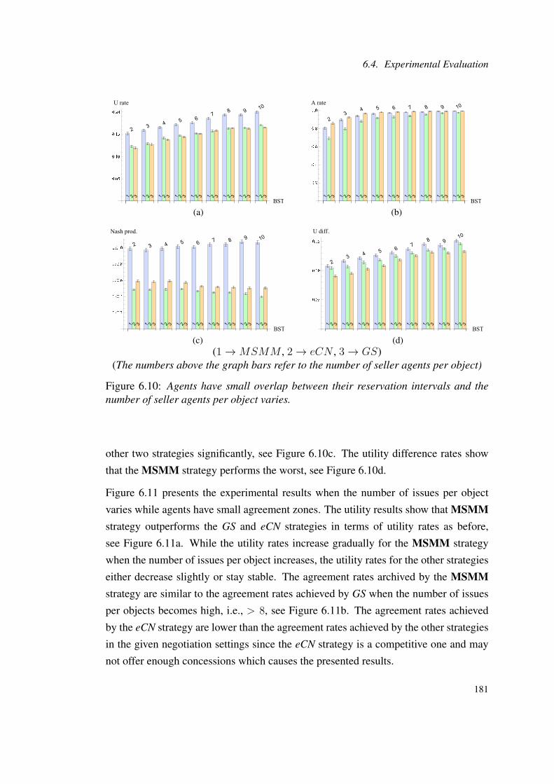
6.4. Experimental Evaluation
(a) (b)
(c) (d)(1→MSMM , 2→ eCN , 3→ GS)
(The numbers above the graph bars refer to the number of seller agents per object)
Figure 6.10: Agents have small overlap between their reservation intervals and thenumber of seller agents per object varies.
other two strategies significantly, see Figure 6.10c. The utility difference rates show
that the MSMM strategy performs the worst, see Figure 6.10d.
Figure 6.11 presents the experimental results when the number of issues per object
varies while agents have small agreement zones. The utility results show that MSMMstrategy outperforms the GS and eCN strategies in terms of utility rates as before,
see Figure 6.11a. While the utility rates increase gradually for the MSMM strategy
when the number of issues per object increases, the utility rates for the other strategies
either decrease slightly or stay stable. The agreement rates archived by the MSMMstrategy are similar to the agreement rates achieved by GS when the number of issues
per objects becomes high, i.e., > 8, see Figure 6.11b. The agreement rates achieved
by the eCN strategy are lower than the agreement rates achieved by the other strategies
in the given negotiation settings since the eCN strategy is a competitive one and may
not offer enough concessions which causes the presented results.
181

Chapter 6. A Single Object with Multiple Negotiation Issues
(a) (b)
(c) (d)(1→MSMM , 2→ eCN , 3→ GS)
(The numbers above the graph bars refer to the number of issues per object)
Figure 6.11: Agents have small overlap between their reservation intervals and thenumber of issues per object varies.
The Nash product rates here are similar to the previous results, see Figures 6.10c and
6.11c. Since the number of seller agents is fixed here (see Section 6.4.2), the utility
difference rates are relatively stable across different number of issues per object for
all the buyer agents, see Figure 6.10d. In addition, the MSMM strategy shows higher
utility difference than the other two strategies in all cases.
The next two sets of experiments show the results when the agreement zone lengths
between buyers and sellers are large. Figure 6.12 shows the results when the number
of seller agents per object varies. Larger agreement zones indicate a better negotiation
environment. The buyer agents are able to achieve higher utility rates than in the
previous set of experiments, see Figures 6.12a and 6.11a. In all cases, the MSMMstrategy performs better than the other strategies in terms of utility rates, see Figure
6.12a. Since the agreement zones are large between agents, all the buyer agents have
no problem in the agreement rates, see Figure 6.12b.
182

6.4. Experimental Evaluation
(a) (b)
(c) (d)(1→MSMM , 2→ eCN , 3→ GS)
(The numbers above the graph bars refer to the number of seller agents per object)
Figure 6.12: Agents have large overlap between their reservation intervals and thenumber of seller agents per object varies.
When the number of sellers per object is less than 4, the MSMM strategy performs
better than the other strategies in terms of the Nash product rates, see Figure 6.12c.
However, when the number of sellers is beyond 4, the strategies MSMM and eCN per-
form similarly. The reason is that the MSMM strategy takes advantage of the situation
when the number of sellers is large. When the number of sellers increases, all strate-
gies produces lower Nash product rates. As Figure 6.12c shows, GS starts to perform
better than the other strategies when the number of sellers per object is more than 4.
Again, the MSMM strategy produces the highest utility difference rates in most cases,
see Figure 6.12d. As the case with the Nash product rates, when the number of seller
agents per object increases, all strategies produces higher utility difference rates. As
before, GS produces the lowest utility difference in most cases.
The last set of experiments in this section is presented in Figure 6.13 where agents have
large agreement zones and the number of issues per object varies. Since the number of
183

Chapter 6. A Single Object with Multiple Negotiation Issues
seller agents per object is fixed in all experiments, results show some stability in their
behaviors. Figure 6.11 shows that the MSMM strategies performs better than the other
two strategies in terms of utility rates, the eCN strategy comes next. As in the previous
set of experiments, the buyer agents have no problem in the reaching agreements for
the same reasons stated before, see Figure 6.13b.
(a) (b)
(c) (d)(1→MSMM , 2→ eCN , 3→ GS)
(The numbers above the graph bars refer to the number of issues per object)
Figure 6.13: Agents have large overlap between their reservation intervals and thenumber of issues per object varies.
The MSMM strategy performs better than the other strategies in terms of Nash product
rates when the number of issues per objects becomes more than 8. The reason is that
when the number of issues per object becomes large, the MSMM strategy starts to offer
their opponents proposals with higher values. When the number of seller agents per
object is less than 8, the MSMM strategy performs either similar to the eCN strategy
or to GS.
Finally, the MSMM strategy performs worse than the other strategies in terms of the
utility difference rates when the number of seller agents per object is less than 9, after
184

6.4. Experimental Evaluation
that, it performs similar or better than the eCN strategy, see Figure 6.13d.
6.4.2.3 Testing Against Mixed-Tactics Dependent Seller Agents
This section tests the performance of the MSMM strategy when the seller agents mix
between the time-dependent tactics and the behavior-dependent tactics to generate their
offers, see Sections 2.3.3.4 and 4.5.2. This sections shows two sets of results. The first
one is when the number of seller agents per object is larger than the number of issues
per object. The second set has the opposite settings. For the two sets of experiments,
the following settings are used: at the start of each negotiation round, the deadlines and
beta values are selected randomly for each seller agent from the intervals [5, 30] and
[0.5, 10] respectively. Similarly, at the start of each negotiation round, two single values
are selected randomly from the intervals [5, 30] and [0.5, 5] and assigned to the buyer
agents as their deadline and β values respectively. Finally, random overlap percentages
are selected from the interval [0% − 100%] for each issue where the seller agents can
have different overlap percentages for the same issue. In the follwoing experimental
results, the SST label on the x-axis stands for the seller strategies.
The first letter in the names of the seller strategies (e.g., PCAS) that are shown on
the x-axis in following experimental results stands for the type of the time-dependent
function the seller agents use to generate the time-dependent part of the final offer,
P stands for polynomial. The second letter stands for the type of the time-dependent
tactic the seller agents use, it can be conceder (C), Boulware (B) or linear L. The
third letter indicates that the seller agents use large portions of the last opponents’
concession to generate the behavior dependent tactic, see Equation 2.9. The last letter
indicates whether the total offer contains small (S) portion of the generated behavior-
dependent offer in the final offer or medium (M) portion, for more information, see
Section 4.5.2
The first experimental results where the number of seller agents per object is 10 and
the number of issues per object is 5 are shown in Figure 6.14. Figure 6.14a shows that
the MSMM strategy performs better than the other strategies in three cases, when the
seller agents play PCAS, PCAM and PLAM while it shows similar utility rates as GS
when the seller agents play PLAS and PBAM since the difference between them are not
statistically significant.
185
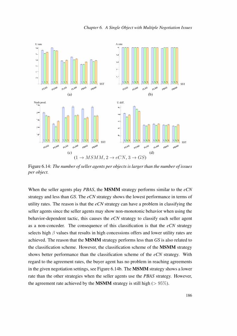
Chapter 6. A Single Object with Multiple Negotiation Issues
(a) (b)
(c) (d)(1→MSMM , 2→ eCN , 3→ GS)
Figure 6.14: The number of seller agents per objects is larger than the number of issuesper object.
When the seller agents play PBAS, the MSMM strategy performs similar to the eCN
strategy and less than GS. The eCN strategy shows the lowest performance in terms of
utility rates. The reason is that the eCN strategy can have a problem in classifying the
seller agents since the seller agents may show non-monotonic behavior when using the
behavior-dependent tactic, this causes the eCN strategy to classify each seller agent
as a non-conceder. The consequence of this classification is that the eCN strategy
selects high β values that results in high concessions offers and lower utility rates are
achieved. The reason that the MSMM strategy performs less than GS is also related to
the classification scheme. However, the classification scheme of the MSMM strategy
shows better performance than the classification scheme of the eCN strategy. With
regard to the agreement rates, the buyer agent has no problem in reaching agreements
in the given negotiation settings, see Figure 6.14b. The MSMM strategy shows a lower
rate than the other strategies when the seller agents use the PBAS strategy. However,
the agreement rate achieved by the MSMM strategy is still high (> 95%).
186
6.4. Experimental Evaluation
The results for the Nash product rates show that the MSMM strategy outperforms the
other strategies in all cases except where the seller agents use the PCAM strategy, see
Figure 6.14c. In addition to the fact that the MSMM strategy offers its opponents
more utility for its proposed counteroffers, it achieves high agreement utilities which
improves the Nash product rates. The exceptional case in the results of the Nash prod-
uct rates can be related to the fact that when the seller agents use the PCAM strategy,
they offer large concessions in the offer generated by the time-dependent tactic which
contributes a medium portion in the final offer. It means that the sellers may reach an
agreement with a very small utility rate which affects the Nash product negatively.
Finally, Figure 6.14d shows the results for the utility difference rates. When the seller
agents use the strategies PCAS or PCAM, the MSMM strategy produces the highest
rates. When the seller agents use any of the other strategies, the MSMM strategies
performs similar to GS or lower where both have higher utility rates than the eCN
strategy. The reason is that the eCN concedes more than the other strategies for the
reason stated in the previous paragraph which makes the difference in the agreement
utilities between the buyers and the sellers small. Moreover, the utility difference
rates for all buyer agents decreases sharply when the seller agents use the any of the
following strategies: PLAS, PLAM, PBAS, PBAM. The reason is the seller agents tend
to offer lower concessions that make the difference in utility smaller than when the
seller agent use any of the other two strategies.
The second set of the experimental results where the number of seller agents per object
is 5 and the number of issues per object is 10 is shown in Figure 6.15. The results
in Figure 6.15 are better than the results shown in Figure 6.14a. The results of the
utility rates here show that MSMM outperforms the other strategies in most cases and
performs similar to GS in only one case, see Figure 6.15a. Since the number of issues
per object in this experiments is higher than the ones in the previous experiments, the
MSMM strategy can secure better utility rates. On the other hand, the MSMM strategy
shows lower agreement rates in few cases, see Figure 6.15b. The reason is that the
number of seller agents per object is lower than before which makes the classification
process used by the MSMM strategy less adaptive in the given negotiation settings.
Again, the agreement rates achieved by the MSMM strategy are still high (≥ 95%).
The Nash product rates here are similar to the Nash product rates shown in Figure
187

Chapter 6. A Single Object with Multiple Negotiation Issues
(a) (b)
(c) (d)(1→MSMM , 2→ eCN , 3→ GS)
Figure 6.15: The number of seller agents per objects is smaller than the number ofissues per object.
6.14c, see Figure 6.15c: the MSMM strategy outperforms the other strategies except
when the seller agents use the PCAM strategy in which GS records higher rates. The
reason for that is explained above. One can note that the Nash product rates shown in
Figure 6.15c are lower than the Nash product rates shown in Figure 6.14c. The reason
is that the number of the seller agents per object in Figure 6.14c is 10 whereas the
number of seller agents per object is 5 in Figure 6.15c. Consequently, the buyer agents
are able to secure higher utility rates when the number of seller agents is high since it
considered a favorable situation for the buyer agents.
Finally, the utility difference rates are shown in Figure 6.15d. The difference between
the utility difference rates of the MSMM strategy and the other strategies are increased
to some extent here when compared to the results shown in Figure 6.14d. Since agents
are assumed to have divergent preferences over issues, the MSMM strategy can gain
more utility per agreement and can also propose counteroffers with more utility to
the opponents in every negotiation round. However since the buyer agent using the
188

6.4. Experimental Evaluation
MSMM strategy negotiates with multiple seller agents, it selects the best acceptable
offer which increases the difference between the agreement utilities of the buyer and
the seller agent.
6.4.2.4 Testing the IOG-conceder Agent
This section compares between the proposed IOG-concession tactic and GS. The GS
is a concession type tactic that concedes on all the issues equally. On the other hand,
the agent uses the IOG-concession tactic starts conceding on the CMII from the oppo-
nent’s point of view, see Section 6.2.
Table 6.4: Experimental settings
Agents or issues per object Deadline descriptionBuyers’
deadlinessellers’
deadlinesBuyers’
beta valuesellers’
beta values OverlapFigurename
Number of agents varies Random deadlines [5-30] [5-30] [0.5-5] [0.5-10] 0%-100% 6.16Number of issues varies Random deadlines [5-30] [5-30] [0.5-5] [0.5-10] 0%-100% 6.17Number of agents varies Equal deadlines [5-30] [5-30] [0.5-5] [0.5-10] 0%-100% 6.18Number of issues varies Equal deadline [5-30] [5-30] [0.5-5] [0.5-10] 0%-100% 6.19
Table 6.4 shows the experimental settings used to generate different results in this
section. It should be mentioned here that the buyer agent uses the IOG-concessiontactic and the buyer agent uses GS propose two counteroffers in every negotiation
round that have the same utility for both agents since they concede the same amount
in terms of utility every time they generate their counteroffers. However, the values of
the issues in the two composite counteroffers can be different, see Section 6.2.
Four sets of results are presented in this section (see Table 6.4) that represent different
negotiation environments. The first set is shown in Figure 6.16. The first set shows the
experimental results when the number of seller agents per object varies and the number
of issues per object is as before, fixed and equals 5. In addition, each seller agent selects
a random deadline from the interval [5, 30] at the start of every negotiation instance. A
deadline is also selected from the same interval at the start of each negotiation instance
and assigned to the buyer agents. The overlap percentage is selected for each issue
randomly form the interval [0%-100%] at the start of each negotiation instance too.
The β values are selected as before.
The above experimental settings are used for all the experiments in this section. The
difference between the settings of difference experiments are in the number of ob-
189

Chapter 6. A Single Object with Multiple Negotiation Issues
(a) (b)
(c) (d)(1→ IOG− concession, 2→ GS)
(The numbers above the graph bars refer to the number of seller agents per object)
Figure 6.16: The number of seller agents per object varies.
jects/issues per object and the deadline which can be either randomly selected as ex-
plained before or be equal for all agents.
The utility rate results are presented in Figure 6.16a. The difference between the two
negotiation tactics in the utility rates are obvious. The IOG-concession tactic per-
forms better than GS because the IOG-concession generates counteroffers with higher
utility values to its opponents than the counteroffers generated by GS. As a result, the
IOG-concession tactic can reach an agreement faster than GS. Both agents concede
at the same rate in terms of utility. If an agent can reach an agreement in negotiation
round, for example, 7, then it can secure a better agreement utility than if it reaches an
agreement at round 8. When the number of seller agents per object increases, the utility
rates for both negotiation tactics increase since more opponents means better oppor-
tunity for the buyer agents to reach agreements with better utilities. The agreements
rates for both buyer agents are the same, see Figure 6.16b.
The Nash product rates are shown in Figure 6.16c. The figure shows that the IOG-
190

6.4. Experimental Evaluation
concession tactic outperforms GS in all cases. The reason for that is the IOG-concessiontactic gains higher utilities for the agreements than GS. In addition, the IOG-concessiontactic provides better counteroffer utilities to its opponents. Both factors increase the
Nash product rates for the IOG-concession tactic. Finally, the utility difference rates
are shown in Figure 6.16d. The figure shows that both tactics achieve similar utility
difference rates. From the results of the previous experiments, and in most cases, GS
shows better performance in terms of the utility difference rates and since the two tac-
tics are concession tactics, they are expected to achieve similar utility difference rates.
As a final observation on the utility difference rates, when the number of seller agents
per object increases, the utility difference rates for both buyer agents increase. When
the number of seller agents is large, they have a better chance to select an agreement
with a higher utility than when the number of seller agents per object is small.
The experimental results when the number of issues per object varies while the number
of seller agents per object is fixed and equals 5 are presented in Figure 6.17. The IOG-concession tactic outperforms GS in terms of utility rates, see Figure 6.17a. When the
number of issues per object increases, both tactics tend to gain less utility rate. The
reason is that the buyer agents need to wait more time to reach the required utility for
the object. Waiting for more time for a concession tactic means less agreement utility
than before. However, when the number of issues per object increases, the difference
between the two utility rates increases since the IOG-concession tactic can benefit
from buyer agents and seller agents having divergent preferences over issues and not
waiting for a longer time before reaching an agreement. In other words, the buyer
agent using GS needs to wait more time than the IOG-concession tactic with every
time the number of issues per object increases. Consequently, it results in bigger gaps
between the utilities of the two tactics when the number of issues per object increases.
As before, both tactics has the same agreement rate which is near 100% in all cases,
see Figure 6.17b.
The Nash product rates are shown in Figure 6.17c. The figure shows that the IOG-concession tactic outperforms GS for the same reasons explained before. As shown
in the figure, the Nash product rates decrease when the number of issues per object
increases for both agents. The reason is that all agents (buyers and sellers) need to wait
more time to reach an agreement which negatively affects the utility of the agreement
for all agents. As the case with the utility rates results, the gaps between the Nash
191
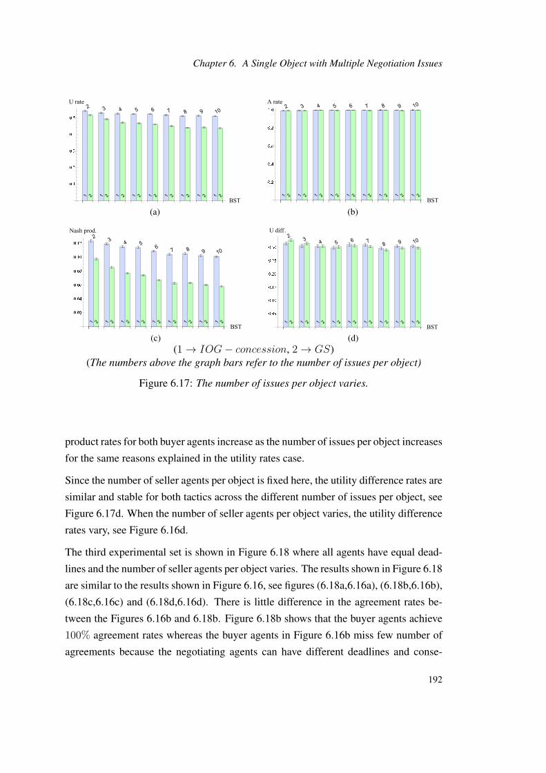
Chapter 6. A Single Object with Multiple Negotiation Issues
(a) (b)
(c) (d)(1→ IOG− concession, 2→ GS)
(The numbers above the graph bars refer to the number of issues per object)
Figure 6.17: The number of issues per object varies.
product rates for both buyer agents increase as the number of issues per object increases
for the same reasons explained in the utility rates case.
Since the number of seller agents per object is fixed here, the utility difference rates are
similar and stable for both tactics across the different number of issues per object, see
Figure 6.17d. When the number of seller agents per object varies, the utility difference
rates vary, see Figure 6.16d.
The third experimental set is shown in Figure 6.18 where all agents have equal dead-
lines and the number of seller agents per object varies. The results shown in Figure 6.18
are similar to the results shown in Figure 6.16, see figures (6.18a,6.16a), (6.18b,6.16b),
(6.18c,6.16c) and (6.18d,6.16d). There is little difference in the agreement rates be-
tween the Figures 6.16b and 6.18b. Figure 6.18b shows that the buyer agents achieve
100% agreement rates whereas the buyer agents in Figure 6.16b miss few number of
agreements because the negotiating agents can have different deadlines and conse-
192
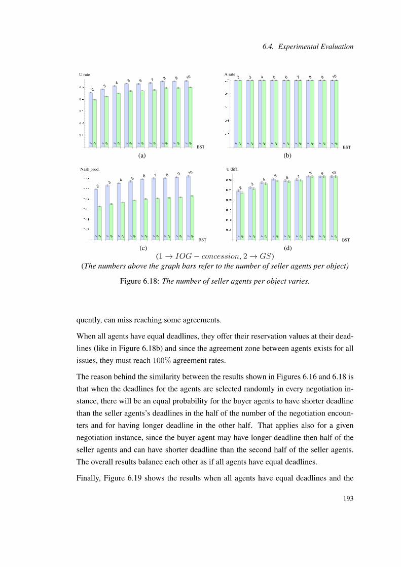
6.4. Experimental Evaluation
(a) (b)
(c) (d)(1→ IOG− concession, 2→ GS)
(The numbers above the graph bars refer to the number of seller agents per object)
Figure 6.18: The number of seller agents per object varies.
quently, can miss reaching some agreements.
When all agents have equal deadlines, they offer their reservation values at their dead-
lines (like in Figure 6.18b) and since the agreement zone between agents exists for all
issues, they must reach 100% agreement rates.
The reason behind the similarity between the results shown in Figures 6.16 and 6.18 is
that when the deadlines for the agents are selected randomly in every negotiation in-
stance, there will be an equal probability for the buyer agents to have shorter deadline
than the seller agents’s deadlines in the half of the number of the negotiation encoun-
ters and for having longer deadline in the other half. That applies also for a given
negotiation instance, since the buyer agent may have longer deadline then half of the
seller agents and can have shorter deadline than the second half of the seller agents.
The overall results balance each other as if all agents have equal deadlines.
Finally, Figure 6.19 shows the results when all agents have equal deadlines and the
193
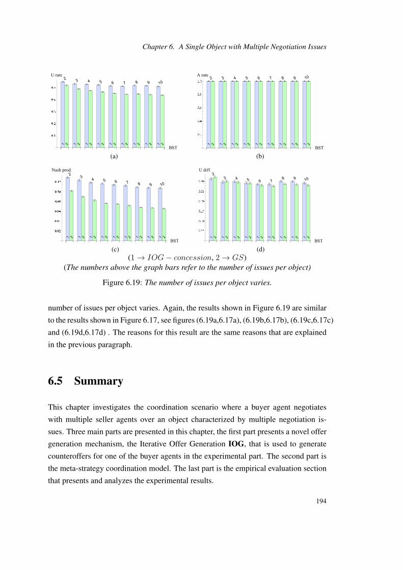
Chapter 6. A Single Object with Multiple Negotiation Issues
(a) (b)
(c) (d)(1→ IOG− concession, 2→ GS)
(The numbers above the graph bars refer to the number of issues per object)
Figure 6.19: The number of issues per object varies.
number of issues per object varies. Again, the results shown in Figure 6.19 are similar
to the results shown in Figure 6.17, see figures (6.19a,6.17a), (6.19b,6.17b), (6.19c,6.17c)
and (6.19d,6.17d) . The reasons for this result are the same reasons that are explained
in the previous paragraph.
6.5 Summary
This chapter investigates the coordination scenario where a buyer agent negotiates
with multiple seller agents over an object characterized by multiple negotiation is-
sues. Three main parts are presented in this chapter, the first part presents a novel offer
generation mechanism, the Iterative Offer Generation IOG, that is used to generate
counteroffers for one of the buyer agents in the experimental part. The second part is
the meta-strategy coordination model. The last part is the empirical evaluation section
that presents and analyzes the experimental results.
194
6.5. Summary
The IOG mechanism includes two negotiation tactics, the IOG-trade-off tactic and
the IOG-concession tactic. Both tactics consider the preferences of the opponents
when generating counteroffers. While staying on the current iso-curve, IOG-trade-offtactic offers more concessions on the issues that are believed to be more important to
the opponents than the others. On the other hand, the IOG-concession tactic concedes
in every negotiation round. It concedes more on the issues that are also believed to be
more important to the opponents than others.
The meta-negotiation model classifies the seller agents into two sets: favorable set and
unfavorable set. The model uses the IOG-trade-off tactic for generating counteroffers
to the favorable set and uses the IOG-concession tactic for generating counteroffers
to the unfavorable set. The IOG-trade-off tactic is used to reach an agreement with
high utility while the IOG-concession tactic is used to guarantee an agreement. The
buyer agent needs to move to a new iso-curve during negotiation when a deadlock
is detected. Once a deadlock is detected, the buyer agent needs to choose new iso-
curve with a lower aspiration level than before. Otherwise, the buyer agent can either
reach an agreement with low utility (via the IOG-concession tactic) or not reaching an
agreement at all.
The distance between the current ios-curve and the new iso-curve is determined by
the lowest first-order difference in the utility offered in the last two negotiation round
amongst the unfavorable group. The results show that when the buyer agent classifies
the seller agents at the start of every negotiation round, the buyer agent gains more
utility than if the seller agents were classified only once at the start of the negotiation
instance.
The last part of the chapter presents and discusses the experimental results. The meta-
strategy is tested with different deadline lengths and with different overlap percentages.
In addition, it is tested against seller agents who mix between the time-dependent tac-
tics and the behavior-dependent tactics when generating their offers.
The results show that the meta-strategy outperforms two benchmark strategies in terms
of the utility rates and the Nash product rates. It also performs equal or better than
the other strategies in terms of the agreement rates. In most cases, the meta-strategy
produces higher utility difference rates than the other two strategies. In addition, it
shows similar results when the seller agents use the mixed strategy to generate their
offers. Moreover, the experimental results show the effect of negotiating with different
195
Chapter 6. A Single Object with Multiple Negotiation Issues
numbers of seller agents per object and with different numbers of negotiation issues
per object.
When the number of seller agents per object increases, all buyer agents produce higher
utility rates, higher agreement rates, higher Nash product rates and higher utility dif-
ference rates. On other other hand, the buyer agents produce the opposite results when
the number of issues per object increases.
The experimental results show that the IOG-concession tactic outperforms a bench-
mark concession negotiation tactic in terms of the utility rates and the Nash product
rates when all agents select random negotiation parameter values (from the same in-
tervals) including the deadlines. In addition, the experimental results show the same
thing when all agents use equal deadlines while other negotiation parameter values are
selected randomly from the same intervals. On the other hand, the two negotiation
tactics show similar results in terms of the agreement rates and the utility difference
rates. The experiments show similar results as before when the number of seller agents
per object and the number of issues per object increase. Moreover, the results show
that there is no significant difference in the results between using equal or random
deadlines for agents.
The meta-strategy negotiation is used in the literature in bilateral negotiation. This
section presents a novel negotiation mechanism that is effective in case of one-to-
many negotiation. The main benchmark strategy that is used to validate the proposed
meta-strategy depends on managing the convexity of the concession curves during
negotiation.
196

Chapter 7
Multiple Objects with MultipleNegotiation Issues
This chapter investigates the coordination scenarios where the number of negotiation
objects are multiple and the number of negotiation issues per object are multiple as
well. Two coordination scenario mechanisms are proposed in this chapter: the mul-
tiple objects multiple issues and single provider (MMS) coordination mechanism and
the global multiple objects multiple issues and multiple providers (MMM) coordina-
tion mechanism. Since there is a single provider per object in the MMS scenario, the
coordination approach is based on managing the local reservation values for the com-
mon issues. The mechanism is tested under different negotiation environments and for
different performance criteria. The experimental results prove that the proposed MMS
coordination mechanism is effective and robust. On the other hand, the global MMM
coordination mechanism populates the local reservation values based on the offers re-
ceived from the opponents in the previous negotiation round. The experimental results
show positive performance by the global MMM mechanism.
7.1 Introduction
Quality-of-service (QoS) attributes are the non-functional characteristics (e.g., through-
put) of a service that distinguish between functionally equivalent services. Providers
of functionally-similar services compete over the non-functional characteristics of ser-
Chapter 7. Multiple Objects with Multiple Negotiation Issues
vices. A competitive criterion in the service oriented domain is the flexibility in the
number of possible QoS attribute options that are available for customers to choose
from. Consider a service with three customizable non-functional QoS attributes such
as throughput, execution time and availability. If that service provider assigns three
possible values for each attribute, then the total number of available configurations
for that service is 27. If the number of service attributes and/or the number of possible
values for each attribute increases then the number of possible service configuration in-
creases and could be intractable. To keep the number of possible service configuration
small, service providers assign small number of possible values for each service at-
tribute. In case of service composition, the possible number of combinations becomes
even larger and less attractable.
The current offer-based methods of QoS assignment show either little or no flexibility
in the possible number of service configurations. An advantage of adopting automated
negotiation as an approach for provisioning/procuring of services is that, when oppo-
nents exchange offers and counteroffers, they direct the search for possible QoS con-
figurations towards their desired preferences by explicitly asking for specific values for
the issues of each service.
Figure 7.1: One-to-many negotiation over multiple object with multiple issues
This chapter investigates the coordination scenario where a buyer agent seeks to pro-
cure multiple objects where each object has multiple issues and a single provider, the
MMS scenario. Figure 7.1 illustrates the MMS scenario. As explained previously, this
situation exists in monopolistic markets where there is a single provider that controls
the supply of a certain market item(s). Moreover, this chapter presents the coordination
scenario where the buyer agent seeks multiple objects with multiple issues and multi-
ple providers, which is a more common scenario than the MMS scenario. Figure 7.2
198

7.2. MMS Coordination Approach
Figure 7.2: Complex one-to-many negotiation
illustrates the MMM scenario. The MMM is the most complex coordination scenario.
Two coordination mechanisms are presented and validated: the MMS coordination
scenario and the global MMM coordination scenario (GMMM).
7.2 MMS Coordination Approach
This section describes the proposed dynamic bidding strategy for the scenario shown
in Figure 7.1, i.e., the MMS strategy. The buyer agent uses the information in each
negotiation thread (i.e., X t−1dil↔sil [Ji]) in the decision making process of adjusting the
weights in the initial IW matrix, see Table 7.1.
Table 7.1: Local reservation value weights (IW)
Service A Service B Service C Service D TotalPrice 0.40 0.25 0.2 0.15 1
Throughput 0.42 0.32 0 0.26 1Response_time 0 0.4 0.25 0.35 1
Reliability 0.40 0.60 0 0 1
Table 7.2: Local reservation values (LR)
Service A Service B Service C Service D Global Reservation ValuesPrice 80 50 40 30 200
Throughput 21 16 0 13 50Response_time 0 16 10 14 40
Reliability 8 12 0 0 20
The proposed coordination strategy is dynamic since it utilizes the different concession
behaviors (levels of cooperation) of the seller agents on each common issue (see Sec-
tion 2.4.2) of each object to adapt the local reservation values for the common issues
199

Chapter 7. Multiple Objects with Multiple Negotiation Issues
in real time, i.e., during negotiation. The MMS strategy adjusts the initial reservation
value weights matrix that will be used to compute a possibly different local reservation
value for each common issue of each service.
The initial reservation value weights matrix (see Table 7.1) could be initialized ac-
cording to the initial reservation value of each issue. The initial reservation values are
usually obtained from domain knowledge or from previous negotiations.
The MMS strategy involves 4 repetitive steps that are repeated in each negotiation
round, see Algorithm 5.
Algorithm 5 MMS()Require: < X t−1
d1,1↔s1,1[j], X t−1
d1,2↔s1,2[j], ..., X t−1
d1,n1↔s1,n1[j] >, ...,
< X t−1dm,1↔sm,1
[j], X t−1dm,2↔sm,2
[j], ..., X t−1dm,mn↔sm,mn
[j] >1: while t <= tmax do2: GroupJ();3: Min_Max_Swap();4: Adjust_Weights();5: Adjust_Local_Res();6: end while
In order to adjust the reservation value weights for the common issues dynamically
during negotiation, we first need to get the recent concession vectors, i.e., the F t−1,t,
see section 4.3. The procedure GroupJ() returns the F t−1,t vector, where [t − 1, t]
is the CTI, see section 4.3. The F t−1,t will be used by the next method, i.e., the
Min_Max_Swap().
The buyer agent starts applying its dynamic negotiation strategy after the first two
negotiation rounds. After executing the GroupJ() algorithm, the MMS Algorithm
executes the Min_Max_Swap() method, see Algorithm 6.
The Min_Max_Swap() algorithm runs into a number of iterations equals to |Ki|/2 and
in each iteration, it swaps between the minimum and maximum values. In each new it-
eration, the previous exchanged values do not undergo a new exchange. In other words,
in each iteration, the algorithm compares between the values that are not swapped in
the previous iterations.
The idea behind the Min_Max_Swap() algorithm is to exploit the fact that different
200

7.2. MMS Coordination Approach
Algorithm 6 Min_Max_Swap()
Require: F t−1,t1: for all (Ki ∈ F t−1,t) do2: for l = 1→ (|Ki|/2) do3: ∆K
′i = Swap(Ki)
4: ∆Ki = K′i
5: end for6: end for7: return F t−1,t
seller agents can have different objectives. For example, some seller agents are desper-
ate for reaching an agreement quickly by offering large amount of concessions while
others prefer to reach an agreement that guarantees high utility and offer small amount
of concessions during negotiation. When the difference between the offers of any two
opponents is maximum, we exchange their values which guarantees that, in the next
negotiation round, the more conceding seller agent receives a counteroffer with less
concession than the counteroffer that will be generated for the less conceding seller
agent. The purpose of this strategy is two folds: first, for agents who are conceding
more, the buyer agent tries to secure an agreement with high utility, secondly, for the
less conceding opponents, the buyer agent tries to secure an agreement regardless the
utility gain as the main objective. The idea of the Min_Max_Swap() algorithm is
explained following example.
• Example: assume that the Ki vector on issue ji at time t is
Kti =< 60, 50, 55, 49, 45, 53, 65, 47 >
Now, we swap between the the minimum and maximum values in the set Kti
over 4 iteration (Kti |/2.) as follows:
– 1st iteration:
(Kti )′=< 60, 50, 55, 49,65, 53,45, 47 >
– 2ed iteration:
(Kti )′′
=< 47, 50, 55, 49,65, 53,45,60 >
– 3rd iteration:
(Kti )′′′
=< 47, 50,49,55,65, 53,45,60 >
201
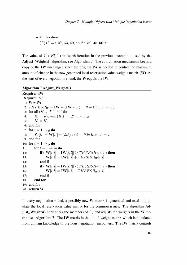
Chapter 7. Multiple Objects with Multiple Negotiation Issues
– 4th iteration:
(Kti )′′′′
=< 47,53,49,55,65,50,45,60 >
The value of kti ((Kti )′′′′) in fourth iteration in the previous example is used by the
Adjust_Weights() algorithm, see Algorithm 7. The coordination mechanism keeps a
copy of the IW unchanged since the original IW is needed to control the maximum
amount of change in the new generated local reservation value weights matrix (W). At
the start of every negotiation round, the W equals the IW.
Algorithm 7 Adjust_Weights()Require: IWRequire: Kt
i
1: W = IW2: THRESHW = IW − (IW ∗ ρ1) // in Exp., ρ1 = 0.33: for all (Ki ∈ F t−1,t) do4: K
′i = Ki/max(Ki) // normalize
5: Ki = K′i
6: end for7: for i = 1→ g do8: W[i, ] = W[i, ]− (∆Fji/ρ2) // in Exp., ρ2 = 29: end for
10: for i = 1→ g do11: for l = 1→ m do12: if (|W[i, l]− IW[i, l]| ≥ THRESHW [i, l]) then13: W[i, l] = IW[i, l] + THRESHW [i, l]14: end if15: if (|W[i, l]− IW[i, l]| < THRESHW [i, l]) then16: W[i, l] = IW[i, l]− THRESHW [i, l]17: end if18: end for19: end for20: return W
In every negotiation round, a possibly new W matrix is generated and used to pop-
ulate the local reservation value matrix for the common issues. The algorithm Ad-just_Weights() normalizes the members of Kt
i and adjusts the weights in the W ma-
trix, see Algorithm 7. The IW matrix is the initial weight matrix which is populated
from domain knowledge or previous negotiation encounters. The IW matrix controls
202

7.2. MMS Coordination Approach
the maximum allowed change to the W matrix. Since different services can have differ-
ent valuations for their issues (attributes), there should be a threshold for the maximum
change. Once the new W is computed, the difference between the IW and W are ad-
justed. It is not expected that the initial IW varies beyond a certain amount in a given
negotiation encounter, which is a realistic assumption. The parameter ρ1 is used to
control the variation amount, see Algorithm 7. A small ρ1 value means a small varia-
tion is allowed and vice versa. In our experiment we use ρ1 = 0.3. The parameter ρ2is used to determine the amount of change to each member in W.
Different ρ2 are tested to find a value that produces good results in the given settings.
As a result, the value of ρ in the experiments was chosen to be 2. The new generated Wmatrix is adjusted before its final use, see lines 10− 19 in Algorithm 7. Lines 10− 19
in Algorithm 7 are important to make sure that the weight of each issue does not differ
from its value in IW beyond the threshold value.
The final step before generating the counteroffers by the buyer agent is to calculate the
new local reservation values by multiplying the global reservation value of each issue
by its new local reservation weight vector in the matrix W.
7.2.1 Experimental Results and Discussion
This section evaluates the coordination approach proposed for the MMS coordination
scenario (see Figure 7.1) where a buyer agent seeks to procure multiple distinct objects
(e.g., services) and each service has multiple issues while there are only one provider
per service. The data shown in Tables 7.1 and 7.2 are used in the experiments of this
section. Table 7.1 shows the local reservation weights for 4 services. Each service has
at least two negotiation issues. Table 7.2 shows the global reservation values for each
issue and the corresponding local reservation value for each issue using the weights in
Table 7.1.
The buyer agent needs to reach an agreement over each object (connected agreement)
to have a successful negotiation outcome. The buyer agents’ utility weight vector used
in the experiments is W =< 0.4, 0.25, 0.2, 0.15 > where the values of the vector
correspond to the following issues in order: 1) price 2) throughput 3) response time
4) reliability. The two types of the buyer agents (the buyer agent using the MMSdynamic strategy and the buyer agent using the general strategy ) use the same utility
203
Chapter 7. Multiple Objects with Multiple Negotiation Issues
weight vector. The utility weight vector for each seller agent is calculated in the start
of each negotiation encounter based on the reservation value of each issue, an issue
with high reservation value gets a high weight.
Some of the negotiation settings in this section are also used in the empirical evaluation
of Section 7.3. The negotiation environment of the experiments is described as follows:
• Offer generation tactics
1. time-dependent tactics:
All seller agents select a β value for the polynomial function [33] from the
same distribution, β ∈ [0.05, 10]. The range of β value covers the three
possible behaviors of an agent, i.e., Boulware where β < 1, linear where
β ≈ 1 and conceder where β > 1.
2. tit-for-tat tactic:
The random absolute tit-for-tat behavior-dependent tactic is used in the
process of generating the mixed offers by the seller agents, δ = 1 and
R(M) = 0 [33]. The percentages of mixing between the time-dependent
tactics and the random absolute tit-for-tat are presented later.
• the experiments compare between a buyer agent using one of the two proposed
coordination strategies (MMS or GMMM) and a buyer agent using the general
strategy (GS).
• at the start of each negotiation encounter which lasts for several rounds, both
buyer agent types are assigned new negotiation parameters, e.g., deadlines. The
non-strategic (i.e., GS) buyer agent keeps its negotiation parameters unchanged
during negotiation while the strategic buyer agent (either using MMS or GMMM)
adapts the local reservation values dynamically during negotiation according to
the behaviors of the current seller agents in terms of their concessions.
• in each negotiation encounter, the two types of the buyer agents play against the
same seller agents
• the error bars are shown for indicating the statistical significance of the results.
• if not stated, the used overlap percentages between the agents’ reservation inter-
vals are randomly selected from the interval [0, 1].
204

7.2. MMS Coordination Approach
The proposed MMS coordination strategy is tested under three different negotiation
environmental factors: deadline, convexity of the concession curve and the type of the
opponent.
7.2.1.1 Negotiation Deadline
Since negotiation deadline is an important negotiation factor given that negotiating
agents must either accept the last received offer/counteroffer or quit negotiation by
the end of their deadlines, deadlines can affect the negotiation outcome since they can
affect both the possibility of reaching an agreement and the utility of an agreement.
This section investigates the performance of the MMS strategy and GS under different
deadlines.
The settings of the experiments are summarized as follows:
• all agents use the time-dependent tactics to generate their offers/counteroffers.
• at the start of each negotiation instance, each seller agent selects a random dead-
line from the interval [5, 60].
• at the start of each negotiation instance, the two types of the buyer agents use the
same selected deadline and the same selected β value. The β value is selected
from the interval [0.05, 2].
The two types of the buyer agents are tested under 10 different deadlines and for
each deadline, the experiment is repeated 1000 times. The term negotiation encounter
here is used to indicate a negotiation attempt. For example, when the buyer agent
needs to procure 4 objects, it needs to start 4 negotiation instances and keeps in ne-
gotiation until an agreement is reached or its deadline is reached. This marks the
end of a negotiation encounter. It was important to clarify this point since the ex-
perimental results present most of the performance criteria as an average per agree-
ment and as an average per encounter. The deadline set used in the experiments is
10, 15, 20, 25, 30, 35, 40, 45, 50, 55. The deadlines are shown on the top of Figures
7.3 and 7.4. The chosen set of deadlines covers small, medium and large deadlines.
Two sets of experimental results are presented here. The first set is related to the utility
rates and agreement rates. The second set is related to the Nash product rates and
utility difference rates, see Section 6.4.2.
205

Chapter 7. Multiple Objects with Multiple Negotiation Issues
Figure 7.3 presents 3 types of results: utility rates per agreement, utility rates per
encounter and agreement rates. As before, the BST label on the x-axis of the figures
stands for the buyers’ strategies.
(a) Utility rate (per agreement) (b) Utility rate (per encounter)
(c) Agreement rate
(1→MMS strategy, 2→ GS)(The numbers above the graph bars refer to the buyer agents’ deadlines)
Figure 7.3: The effect of different deadlines on the utility rate and the agreement rate
Figures 7.3a and 7.3b show that the MMS strategy outperforms GS in terms of the
utility rate per agreement and the utility rate per encounter across all deadlines. When
the deadlines are short or large, the utility rates are relatively smaller than the utility
rates when the deadlines are in the middle of the interval for both buyer agents, i.e., for
the buyer agent uses the MMS strategy and the buyer agent uses GS. The reason is that
when the buyers’ deadlines are short or large, the seller agents’ deadlines are selected
short or large with small probabilities. As a consequence, the number of agreements
are smaller because agents may reach their deadlines and quit negotiations without
reaching an agreement. Since similar trends are shown in the following experimental
results, this explanation is valid for all the following similar results.
206
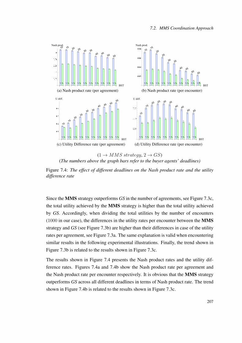
7.2. MMS Coordination Approach
(a) Nash product rate (per agreement) (b) Nash product rate (per encounter)
(c) Utility Difference rate (per agreement) (d) Utility Difference rate (per encounter)
(1→MMS strategy, 2→ GS)(The numbers above the graph bars refer to the buyer agents’ deadlines)
Figure 7.4: The effect of different deadlines on the Nash product rate and the utilitydifference rate
Since the MMS strategy outperforms GS in the number of agreements, see Figure 7.3c,
the total utility achieved by the MMS strategy is higher than the total utility achieved
by GS. Accordingly, when dividing the total utilities by the number of encounters
(1000 in our case), the differences in the utility rates per encounter between the MMSstrategy and GS (see Figure 7.3b) are higher than their differences in case of the utility
rates per agreement, see Figure 7.3a. The same explanation is valid when encountering
similar results in the following experimental illustrations. Finally, the trend shown in
Figure 7.3b is related to the results shown in Figure 7.3c.
The results shown in Figure 7.4 presents the Nash product rates and the utility dif-
ference rates. Figures 7.4a and 7.4b show the Nash product rate per agreement and
the Nash product rate per encounter respectively. It is obvious that the MMS strategy
outperforms GS across all different deadlines in terms of Nash product rate. The trend
shown in Figure 7.4b is related to the results shown in Figure 7.3c.
207

Chapter 7. Multiple Objects with Multiple Negotiation Issues
The utility difference rate results are presented in Figures 7.4c and 7.4d. The MMSstrategy shows higher utility difference rates in both figures. The results indicates that
the fairness of the agreements is affected negatively when using the MMS.
The results above prove the effectiveness of the MMS strategy in managing the local
reservation values of the common issues under different deadlines to achieve positive
results in terms of the utility rate, the agreement rate and the Nash product rate.
7.2.1.2 Convexity of the Concession Curve
The convexity of a curve refers to the degree of its curvature. The convexity can affect
the amount of concessions offered. Changing the convexity of a concession curve dur-
ing negotiation affects the amount of concession offered at the next negotiation round.
Experiments are designed and implemented to test the effect of different concession
curve convexities on the performance of the buyers’ strategies.
The experimental setups here are similar to the ones in Section 7.2.1.1 except for the
buyers’ deadlines and the β values. Since the β value determines the convexity of the
concession curve, the two types of the buyer agents are tested under different β values.
The set of β values used in the experiments is 0.3, 0.6, 0.8, 1, 1.2, 1.5, 2, 3, 4, 5which
appears on the top of Figures 7.5 and 7.6. The set covers wide range of concession
behaviors including tough, linear and conceder. A random deadline is selected from
the interval [5, 60] and assigned to the buyer agents at the start of every negotiation
instance.
In the start of each negotiation instance, the two buyer agents use the same β value
throughout negotiation and for each β value, the experiment is repeated 1000 times.
As the case before, two experimental sets are presented in this section. The first set
shows the utility rate and the agreement rate results while the second set shows the
Nash product rate and the utility difference rate results.
The first set of the results are shown in Figure 7.5. The utility rate per agreement and
the utility rate per encounter results are shown in Figures 7.5a and 7.5b respectively.
The results show that the MMS strategy outperforms GS in terms of utility rate across
all β values. Both buyer agents show lower utility rates when β values decrease. The
reason is that with the increase in the values of β, the buyer agent offers more and more
concessions. As a consequence, its utility per agreement gets smaller and smaller.
208
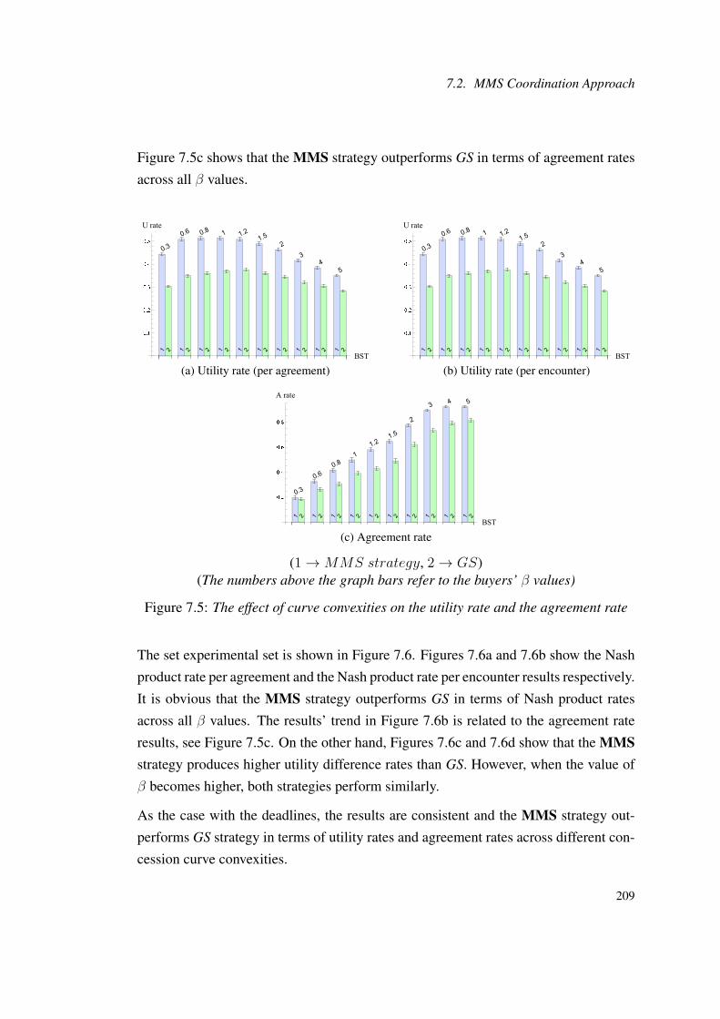
7.2. MMS Coordination Approach
Figure 7.5c shows that the MMS strategy outperforms GS in terms of agreement rates
across all β values.
(a) Utility rate (per agreement) (b) Utility rate (per encounter)
(c) Agreement rate
(1→MMS strategy, 2→ GS)(The numbers above the graph bars refer to the buyers’ β values)
Figure 7.5: The effect of curve convexities on the utility rate and the agreement rate
The set experimental set is shown in Figure 7.6. Figures 7.6a and 7.6b show the Nash
product rate per agreement and the Nash product rate per encounter results respectively.
It is obvious that the MMS strategy outperforms GS in terms of Nash product rates
across all β values. The results’ trend in Figure 7.6b is related to the agreement rate
results, see Figure 7.5c. On the other hand, Figures 7.6c and 7.6d show that the MMSstrategy produces higher utility difference rates than GS. However, when the value of
β becomes higher, both strategies perform similarly.
As the case with the deadlines, the results are consistent and the MMS strategy out-
performs GS strategy in terms of utility rates and agreement rates across different con-
cession curve convexities.
209

Chapter 7. Multiple Objects with Multiple Negotiation Issues
(a) Nash product rate (per agreement)
1 2
0.3
1 2
0.6
1 2
0.8
1 2
1
1 2
1.2
1 2
1.5
1 2
2
1 2
3
1 2
4
1 2
5
BST
0.02
0.04
0.06
0.08
0.10
Nash prod.
(b) Nash product rate (per encounter)
(c) Utility Difference rate (per agreement) (d) Utility Difference rate (per encounter)
(1→MMS strategy, 2→ GS)
Figure 7.6: The effect of curve convexities on the Nash product rate and the utilitydifference rate
7.3 MMM Coordination approach
This section investigates the scenario shown in Figure 7.2 where a buyer agent is nego-
tiating with multiple seller agents over multiple distinct objects given that each agent
has multiple issues and multiple providers. The situation for the buyer agent is more fa-
vorable in the case of the MMM scenario than the MMS scenario since there are many
seller agents competing for each object. Algorithm 8 summarizes the proposed global
coordination mechanism, the GMMM mechanism. The GMMM (global multiple ob-
jects, multiple issues and multiple providers) mechanism does not require an initial
W matrix (see Table 7.1) to start with in case the seller agents start proposing the of-
fers. The matrix W for the next negotiation round is defined dynamically based on the
received offers in the previous round.
The GMMM mechanism is explained as follows: first, it groups the last received
210
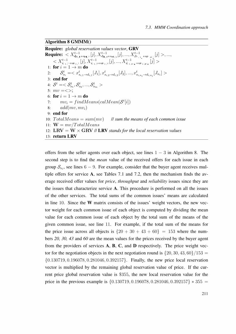
7.3. MMM Coordination approach
Algorithm 8 GMMM()Require: global reservation values vector, GRVRequire: < X t−1
d1,1↔s1,1[j], X t−1
d1,2↔s1,2[j], ..., X t−1
d1,n1↔s1,n1[j] >, ...,
< X t−1dm,1↔sm,1
[j], X t−1dm,2↔sm,2
[j], ..., X t−1dm,mn↔sm,mn
[j] >1: for i = 1→ m do2: Stoi =< xtsi,1→di,1 [J1], x
tsi,2→di,2 [J2], ..., x
tsi,ni→di,ni
[Jni ] >
3: end for4: St =< Sto1 ,S
to2, ...,Stom >
5: mv =<>;6: for i = 1→ m do7: mvi = findMeans(calMean(St[i])8: add(mv,mvi)9: end for
10: TotalMeans = sum(mv) // sum the means of each common issue11: W = mv/TotalMeans12: LRV = W ×GRV // LRV stands for the local reservation values13: return LRV
offers from the seller agents over each object, see lines 1 − 3 in Algorithm 8. The
second step is to find the mean value of the received offers for each issue in each
group Soi , see lines 6 − 9. For example, consider that the buyer agent receives mul-
tiple offers for service A, see Tables 7.1 and 7.2, then the mechanism finds the av-
erage received offer values for price, throughput and reliability issues since they are
the issues that characterize service A. This procedure is performed on all the issues
of the other services. The total sums of the common issues’ means are calculated
in line 10. Since the W matrix consists of the issues’ weight vectors, the new vec-
tor weight for each common issue of each object is computed by dividing the mean
value for each common issue of each object by the total sum of the means of the
given common issue, see line 11. For example, if the total sum of the means for
the price issue across all objects is 20 + 30 + 43 + 60 = 153 where the num-
bers 20, 30, 43 and 60 are the mean values for the prices received by the buyer agent
from the providers of services A, B, C, and D respectively. The price weight vec-
tor for the negotiation objects in the next negotiation round is 20, 30, 43, 60/153 =
0.130719, 0.196078, 0.281046, 0.392157. Finally, the new price local reservation
vector is multiplied by the remaining global reservation value of price. If the cur-
rent price global reservation value is $355, the new local reservation value for the
price in the previous example is 0.130719, 0.196078, 0.281046, 0.392157 ∗ 355 =
211
Chapter 7. Multiple Objects with Multiple Negotiation Issues
46.4052, 69.6078, 99.7712, 139.216. The previous vector can be interpreted as: the
current price local reservation value for service A is $46.4052 and the current price
local reservation value for service B is $69.6078 etc. This process is repeated for the
other issues. As line 12 shows, the new W matrix is multiplied by the vector of the re-
maining global reservation values GRV. The local reservation (LR) matrix is returned
by the algorithm. Finally, the buyer agent uses possibly a new local reservation value
for each issues of each object in every negotiation round as the algorithm is repeated
at the start of every negotiation round.
Since the buyer agent receives multiple offers for each issue, then taking the mean
value for the received offers and then normalizes all the mean value vectors for all
issues provides a good approximation for the demand and importance of each issue
to a particular seller group. Consequently, the dynamic adaptation of the W matrix
responds to the behaviors of the seller agents in terms of their concessions on various
issues.
The proposed mechanism in Algorithm 8 is one of the possible ways for coordinating
the bidding strategy at the global level in the given scenario. However, other mech-
anisms that work under different assumptions need to be designed and tested. For
example, in case the buyer agent has an initial local reservation weight matrix and the
amount of resource shifting between delegates cannot go beyond a certain amount for
each issue, then the shifting of resources according to the behaviors of the seller agents
over the common issues amongst delegates is the suitable approach in this case. In
addition, a local coordination mechanism is essential for using a hybrid coordination
mechanism since the empirical results in Chapter 5 show that the hybrid coordination
mechanism outperforms other coordination mechanisms in terms of the utility rates
and the agreement rates.
7.3.1 Experimental Results and Discussion
This section tests the GMMM strategy under four negotiation variables: deadline,
convexity of the concession curve, number of available seller and finally length of the
agreement zone.
212

7.3. MMM Coordination approach
7.3.1.1 Negotiation Deadline
The experimental settings here are similar to the settings mentioned in section 7.2.1.1.
The difference here is that the number of the seller agents per object is set to 5. The
numbers shown above bars in the following graphs indicate the buyer agents’ dead-
lines. The seller agents select their deadlines as explained in section 7.2.1.1.
(a) Utility rate (per agreement) (b) Utility rate (per encounter)
(c) Agreement rate
(1→ GMMM strategy, 2→ GS)(The numbers above the graph bars refer to the buyer agents’ deadlines)
Figure 7.7: The effect of different deadlines on the utility rate and the agreement rate
The first set of results is shown in Figure 7.7. Figures 7.7a and 7.7b show that the
GMMM strategy outperforms GS significantly in terms of the utility rate per agree-
ment and the utility rate per encounter results. Since the number of the providers per
object are multiple, achieving a good agreement rate is not a problem for both strate-
gies, see Figure 7.7c. Since the number of the seller agents per object is multiple in
the MMM scenario, it is expected that the buyer agents benefit from the situation and
gain higher utility rates than in the MMS scenario, see Figures 7.3a and 7.7a.
The Nash product rate and the utility difference rate results are presented in Figure
213
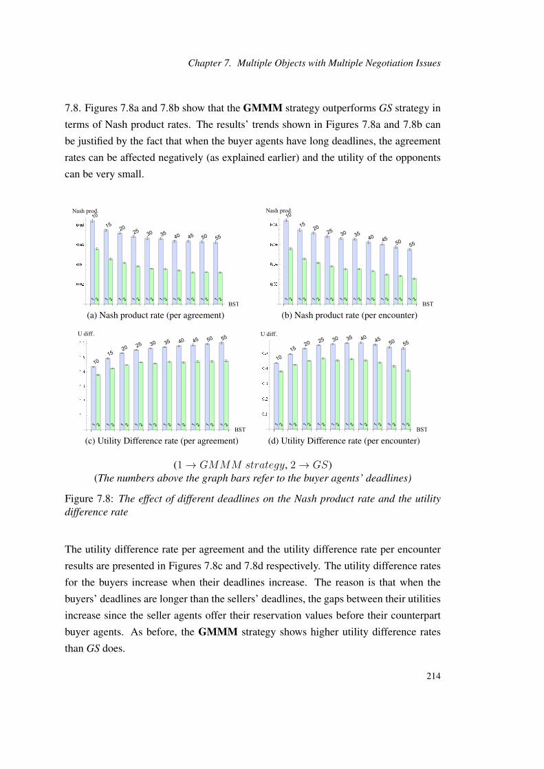
Chapter 7. Multiple Objects with Multiple Negotiation Issues
7.8. Figures 7.8a and 7.8b show that the GMMM strategy outperforms GS strategy in
terms of Nash product rates. The results’ trends shown in Figures 7.8a and 7.8b can
be justified by the fact that when the buyer agents have long deadlines, the agreement
rates can be affected negatively (as explained earlier) and the utility of the opponents
can be very small.
(a) Nash product rate (per agreement) (b) Nash product rate (per encounter)
(c) Utility Difference rate (per agreement) (d) Utility Difference rate (per encounter)
(1→ GMMM strategy, 2→ GS)(The numbers above the graph bars refer to the buyer agents’ deadlines)
Figure 7.8: The effect of different deadlines on the Nash product rate and the utilitydifference rate
The utility difference rate per agreement and the utility difference rate per encounter
results are presented in Figures 7.8c and 7.8d respectively. The utility difference rates
for the buyers increase when their deadlines increase. The reason is that when the
buyers’ deadlines are longer than the sellers’ deadlines, the gaps between their utilities
increase since the seller agents offer their reservation values before their counterpart
buyer agents. As before, the GMMM strategy shows higher utility difference rates
than GS does.
214

7.3. MMM Coordination approach
7.3.1.2 Convexity of the Concession Curve
The settings here are similar to the setting in section 7.2.1. Again, the difference is
that buyer agents use a certain β value in each negotiation encounter while all other
parameters are selected randomly as explained earlier. Changing the convexity of the
concession curve affects the amount of concession offered at a particular round.
(a) Utility rate (per agreement) (b) Utility rate (per encounter)
(c) Agreement rate
(1→ GMMM strategy, 2→ GS)(The numbers above the graph bars refer to the buyers’ β values)
Figure 7.9: The effect of different buyers’ β values on the utility rate and the agreementrate
To test the effect of using different convexity degrees for the buyers’ concession curve,
we test the proposed strategy under different curve convexities. The value β in the time
dependent-offer generation tactic affects the convexity of the concession curve. The
values of β used in the experiments are shown on the top of Figures 7.9 and 7.10.
The results in Figure 7.9 show that the GMMM outperforms GS in terms of the utility
rate per agreement (see Figure 7.9a) and the utility rate per encounter, see Figure 7.9b.
215

Chapter 7. Multiple Objects with Multiple Negotiation Issues
When the β values become large, the utility rates for the buyer agents decrease. How-
ever, the GMMM outperforms GS in all cases. Both strategies perform similarly in
terms of the agreement rate (see Figure 7.9c) since the number of the seller agents per
object is multiple and the chance of reaching an agreement is high. When the buyer
agents have very small β values, they miss some agreements since they concede in
very small amounts which makes reaching an agreement more difficult. However, the
GMMM performs similar or better than GS in all cases.
(a) Nash product rate (per agreement) (b) Nash product rate (per encounter)
(c) Utility Difference rate (per agreement) (d) Utility Difference rate (per encounter)
(1→ GMMM strategy, 2→ GS)(The numbers above the graph bars refer to the buyers’ β values)
Figure 7.10: The effect of different buyers’ β values on the utility rate and the agree-ment rate
The Nash product rate and the utility difference rate results are shown in Figure 7.10.
Figures 7.10a and 7.10b show that the GMMM outperforms GS in terms of the Nash
product rate per agreement and the Nash product rate per encounter.
When the β values becomes large, Nash product rate increases for both strategies since
a conceder agent tends to offer more concessions and hence the opponents gain higher
216

7.3. MMM Coordination approach
agreement utilities. The utility difference rate results are shown in Figures 7.10c and
7.10d. As before, the GMMM strategy produces high utility difference rates when
compared to the utility difference rates produced by GS.
7.3.1.3 Number of the Seller Agents per Object
In this section, we investigate how the initial number of seller agents per a negotia-
tion object can affect the negotiation results. The experimental settings are similar to
the settings discussed in section 7.2.1. The two buyer agents use the same randomly
selected parameters such as deadline and β since we are testing only for the number
of seller agents per object. The numbers of the seller agents per object are shown on
the above of the bars in Figures 7.11 and 7.12. The experiments started with 2 seller
agents per objects and increased up to 11 seller agents per object.
(a) Utility rate (per agreement) (b) Utility rate (per encounter)
(c) Agreement rate
(1→ GMMM strategy, 2→ GS)(The numbers above the graph bars refer to the number of seller agents per object)
Figure 7.11: The effect of different number of sellers on the utility rate and the agree-ment rate
217
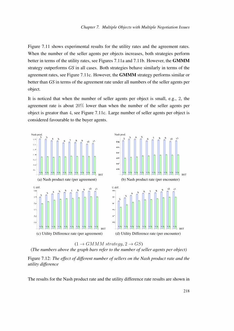
Chapter 7. Multiple Objects with Multiple Negotiation Issues
Figure 7.11 shows experimental results for the utility rates and the agreement rates.
When the number of the seller agents per objects increases, both strategies perform
better in terms of the utility rates, see Figures 7.11a and 7.11b. However, the GMMMstrategy outperforms GS in all cases. Both strategies behave similarly in terms of the
agreement rates, see Figure 7.11c. However, the GMMM strategy performs similar or
better than GS in terms of the agreement rate under all numbers of the seller agents per
object.
It is noticed that when the number of seller agents per object is small, e.g., 2, the
agreement rate is about 20% lower than when the number of the seller agents per
object is greator than 4, see Figure 7.11c. Large number of seller agents per object is
considered favourable to the buyer agents.
(a) Nash product rate (per agreement) (b) Nash product rate (per encounter)
(c) Utility Difference rate (per agreement) (d) Utility Difference rate (per encounter)
(1→ GMMM strategy, 2→ GS)(The numbers above the graph bars refer to the number of seller agents per object)
Figure 7.12: The effect of different number of sellers on the Nash product rate and theutility difference
The results for the Nash product rate and the utility difference rate results are shown in
218
7.3. MMM Coordination approach
Figure 7.12. The results for the Nash product rate per agreement and the Nash product
rate per encounter results are shown in Figures 7.12a and 7.12b respectively. The Nash
product rates show that the GMMM strategy outperforms GS significantly in both
graph results. When the number of the seller agents increases, the utility agreement of
the opponents can be lower which affects the Nash product rate, see Figure 7.12a.
The utility difference rate results are presented in Figures 7.12c and 7.12d. The re-
sults here are consistent as before. When the number of the seller agents per object
increases, both strategies tend to have larger utility rate differences. The reason is that
when the number of the seller agents are large, the buyer agents benefit from this situ-
ation and gain higher utility rates than when the number of seller agents per object is
smaller.
7.3.1.4 Length of the Agreement Zone
The length of the agreement zone between opponent agents can affect the negotiation
outcomes. This section tests the buyers’ strategies under different overlap percentages
(i.e., different agreement zone lengths) between the reservation intervals of the objects’
issues. For example, assume that the reservation interval for a buyer agent for price is
[5, 20]. It means the initial offer for that agent is $5 and the maximum price (reservation
value) is $20. If the opponent agent has the same reservation interval too, i.e., [5, 20]
where the starting offer is $20 and the minimum price (its reserve price) is $5, then
the two agents have 100% overlap and the agreement zone is the longest possible. To
see how the overlap percentage affect the negotiation results for the two strategies, the
follwoing experimental aresults are presented and discussed. For more information
about the overlap percenages, see Section 4.5.2.
Three types of overlap percentages are used in the experiments: small (5%- 25%),
medium (30%- 60%) and large overlap (70%- 100%). The results indicate that when
the overlap is large (i.e., the agreement zone is large), the negotaion outcome are posi-
tively affected and vice versa, see Figure 7.13 and 7.14.
Figure 7.13 presents the utility rate and the agreement rate results. The GMMM strat-
egy outperforms GS in terms of utility rates, see Figures 7.13a and 7.13b. In addi-
tion, the GMMM strategy outperforms GS in terms of the agreement rates in case the
agreement zones are small and medium, see Figures 7.13c. When the agreement zone
219

Chapter 7. Multiple Objects with Multiple Negotiation Issues
(a) Utility rate (per agreement) (b) Utility rate (per encounter)
(c) Agreement rate
(1→ GMMM strategy, 2→ GS)
Figure 7.13: The effect of different agreement zone lengths on the utility rate and theagreement rate
is large, both strategies perform similarly.
The Nash product rate and the utility difference rate results are presented in Figure
7.14. The results here are consistent with the results presented earlier. The GMMMstrategy outperforms GS in terms of the Nash product rates, see Figures 7.14a and
7.14b. As the case with the utility rates and the agreement rates, when the agreement
zone gets larger, both strategies perform better. In addition, the GMMM strategy
produces higher utility rate differences than the utility rate differences produced by
GS, see Figures 7.14c and 7.14d.
In general, when the agreement zones between agents increase, both strategies produce
better results.
220

7.4. Summary
(a) Nash product rate (per agreement) (b) Nash product rate (per encounter)
(c) Utility Difference rate (per agreement) (d) Utility Difference rate (per encounter)
(1→ GMMM strategy, 2→ GS)
Figure 7.14: The effect of different agreement zone lengths on the Nash product rateand the utility difference rate
7.4 Summary
This chapter investigates the coordination scenarios where the number of distinct ne-
gotiation objects is multiple and the number of negotiation issues per object is multiple
too. First, a coordination mechanism is proposed for the MMS coordination scenario
where each object has a single provider. This scenario exists in monopolistic markets
where there is a single provider that controls the supply of a certain market item(s). On
the other hand, a global coordination mechanism is proposed for the MMM coordina-
tion scenario where each object has multiple issues and multiple prospective providers.
The MMS coordination strategy manipulates the local reservation values for the com-
mon issues of the different objects. The seller agents’ concessions on the common
issues are analyzed and every common issue is assigned a possibly new reservation
value accordingly. The coordination mechanism is repeated at the start of every ne-
gotiation round. The mechanism is validated empirically under different negotiation
221
Chapter 7. Multiple Objects with Multiple Negotiation Issues
environments. It is compared with the general negotiation strategy where the negoti-
ation variables are initialized at the start of every negotiation encounter and kept un-
changed. The MMS and general strategies are tested under different deadline lengths
and different concession curve convexities. The MMS strategy outperforms the gen-
eral strategy significantly in terms of the utility rates, the Nash product rates and the
agreement rates. The MMS strategy are proven to be effective and robust in the given
negotiation environments. Finally, it produces higher utility difference rates than the
utility difference rates produced by the general strategy.
To manage the bidding strategy for the MMM coordination scenario, a global coordi-
nation mechanism is proposed. The GMMM strategy manages the local reservation
values based on the values of the last opponents’ offers. The global strategy does
not require an initial local reservation value matrix if the seller agents start proposing.
At the start of the every negotiation round, the GMMM strategy constructs the local
reservation value matrix from the last sets of the received offers. An initial set of exper-
imental results are presented. The proposed strategy is tested under different deadline
lengths, under different concession curve convexities, under different numbers of seller
agents per object and under difference agreement zone lengths. The results show that
the GMMM strategy outperforms the general strategy in terms of the utility rates, the
Nash product rates and performs similar or better in terms of the agreement rates. As
in the MMS strategy case, the GMMM strategy shows higher utility difference rates
than the ones produced by the general strategy.
The GMMM strategy shows higher utility rates and lower Nash product rates than the
ones shown by the MMS strategy because the GMMM strategy benefits from existing
multiple providers per object. Finally, the proposed mechanisms are compared with the
general strategy because the coordination scenario presented in this chapter is rarely
investigated in the literature.
222

Chapter 8
Conclusion
This thesis investigates the bidding negotiation strategies in the one-to-many negotia-
tion where a buyer agent negotiates concurrently with multiple seller agents. The main
assumptions here are that the agents negotiate under incomplete knowledge where the
preferences over the outcomes, the utility structure, the offer generation tactics and the
deadlines are considered private information for each agent.
To classify different negotiations, the three main negotiation components and their
numbers are considered: the number of negotiation objects which is equivalent to the
number of the required agreements in our case, the number of negotiation issues per
object and the number of providers (seller agents) per object. Accordingly, the one-to-
many negotiation is classified into five different coordination scenarios, namely: SSM,MSM, SMM, MMS, MMM, where S stands for single and M stands for multiple.
The first letter refers to the number of negotiation objects, the second letter refers to
the number of issues per object and the third letter refers to the number of providers
per object. For example, the SSM scenario indicates the situation where a buyer agent
seeks to procure a single object characterized by a single issue and there are many
available providers willing to provision that object. Each one-to-many coordination
scenario is investigated and one or more novel dynamic bidding mechanism(s) (dy-
namic negotiation strategy(s)) are proposed. Since the main problem addressed in this
thesis is to coordinate the bidding strategies for multiple concurrent negotiations dur-
ing negotiation, i.e, real-time coordination, the proposed solution approach base its
coordination decisions on the level of cooperation of the current opponents in terms of
their concessions in the current negotiation. The coordination mechanisms presented

Chapter 8. Conclusion
in this thesis do not consider any historical information since the negotiations are as-
sumed to be as a one-off type. Accordingly, all the proposed bidding strategies are
characterized by their dynamicity that depends only on the current behaviors of the
seller agents in terms of their concessions in the current negotiation. The proposed
coordination mechanisms for the one-to-many negotiation consider managing the ne-
gotiation variables (e.g., convexity of the concession curve) during negotiation. The
collection of the negotiation variables and their values represent the current negotiation
strategy for an agent. The proposed bidding strategies are empirically validated against
the state-of-the-art negotiation strategies. The next few paragraphs discuss briefly the
proposed mechanism(s) for each coordination scenario.
For the SSM coordination scenario, where a buyer agent seeks to procure a single ob-
ject (e.g., a service) characterized by a single issue (e.g., price) and many providers
for that object exist, a dynamic negotiation strategy is proposed to manage the buyer
agent’s concession curve convexities (each buyer’s delegate can have a different con-
cession curve convexity) during negotiation. The decision making mechanism for man-
aging the convexity curves during negotiation depend on the collective behaviors of
the current opponents. In each negotiation round, the behaviors of the current seller
agents are analyzed and a new convexity is assigned to each concession curve of each
delegate. The proposed negotiation strategy is tested against 4 different negotiation
strategies. One is a general strategy where its negotiation parameter values (e.g., con-
cession curve convexity) are initialized at the start of negotiation and stay without any
change throughout negotiation and quit negotiation as soon as it reaches an agreement.
The second strategy keeps negotiating until it reaches its deadline then selects the best
acceptable agreement. The last two strategies adjust either the convexity curve or the
reservation value during negotiation. All strategies are tested in different negotiation
environments. The experimental results show that the proposed negotiation strategy
outperforms the benchmark strategies in terms of the utility rates and performs similar
or better in terms of the agreement rates in most situations.
Different measures can be used to evaluate the behaviors of the current opponents dur-
ing negotiation: early concessions, most recent concessions and utilities of the last
offers. In addition, any combination between the measures can also be used to evalu-
ate the behaviors of the opponents. For example, the experiments that are conducted
to evaluate the proposed coordination mechanism for the SSM scenario evaluate the
224
current opponents by using 50% from the utilities of the last offers measure and 50%
from the most recent concessions measure. A set of experiments are designed to eval-
uate each measure empirically. The experimental results show that (in most cases)
the recent concessions measure performs similar or better than the other evaluation
criteria.
The MSM coordination scenario is a negotiation scenario where a buyer agent seeks
to procure multiple distinct objects (e.g., multiple services) where each object has a
single issue (e.g., price) and multiple providers. Three coordination mechanisms are
proposed: global coordination mechanism, local coordination mechanism and hybrid
coordination mechanism. The global coordination mechanism manages the local reser-
vation value for each issue of each object during negotiation taking into consideration
the behaviors of all the seller agents, i.e., global view. The local coordination mecha-
nism manages the convexity of the concession curve for a set of delegates of a given
object. In other words, in the local coordination mechanism, the behaviors of the
providers of a certain object are analyzed without considering the behaviors of the
providers of other objects, hence the name local. Finally, the hybrid mechanism com-
bines both, the global mechanism and the local mechanism. To generate counterof-
fers in every negotiation round, the hybrid coordination mechanism receives new local
reservation values from the global strategy and receives the convexity of the conces-
sion curve for each set of delegates (of a given object) from the local strategies since
there would be local strategies equal to the current number of the negotiation objects.
Under tough negotiation environments where the length of agreement zones between
agents are small, the experimental results show that the global strategy outperforms
the general strategy and a state-of-the-art negotiation strategy (that manages the local
reservation values) in terms of the agreement rates and performs similar or better than
the state-of-the-art strategy in terms of the utility rates. The local strategy achieves
better utility rates than the benchmark strategies. The hybrid strategy outperforms all
strategies, including both, the global and local strategies, in terms of both, the utility
rates and the agreement rates.
Since the SMM coordination scenario considers a situation where a buyer agent seeks
to procure an object characterized by multiple negotiation issues and the number of
the providers is multiple, a meta-strategy model is proposed that alternates between a
concession tactic and a trade-off tactic during negotiation. In addition, a novel iter-
225
Chapter 8. Conclusion
ative offer generation mechanism is proposed and used to generate counteroffers for
the buyer agent. It includes two negotiation tactics, the IOG-trade-off tactic and IOG-
concession tactic. Whether the buyer agent decides to use the IOG-concession tactic
or the IOG-trade-off tactic, it starts offering concessions on the issues that are believed
to be more important to the opponent. This way of offering concessions helps reach an
agreement quickly and improves the social welfare of the system. The meta-strategy is
tested against two other benchmark negotiation strategies. The first one is the general
strategy (sometimes called tactic) and the second is a strategy that manages the con-
vexity of the concession curves. Four different performance criteria are considered in
the experiments: utility rate, agreement rate, Nash product rate and utility difference
rate. The Nash product rate measures the social welfare while the utility difference
rate assesses the fairness of an agreement. A set of experiments are designed and im-
plemented to evaluate the meta-strategy under different negotiation environments. The
experimental results show that the meta-strategy performs better than the benchmark
strategies in terms of the utility rates and the Nash product rates. It also performs sim-
ilar or better than the benchmark strategies in terms of the agreement rates. In most
cases, the meta-strategy shows equal or higher utility difference rates than the bench-
mark strategies. In addition, the experiments show that all strategies perform better
in terms of the utility rates, the agreement rates and the Nash product rates when the
number of the seller agents per object is large. On the other hand, the opposite re-
sults (except for agreement rates) are noticed when the number of the issues per object
is large. Moreover, a second set of experiments is dedicated to evaluate the IOG-
concession tactic against the general strategy that is considered as a concession tactic.
Under different deadlines, the IOG-concession tactic outperforms the general strategy
in terms of the utility rates and the Nash product rates. Both tactics perform similar in
terms of the agreement rates and the utility difference rates.
The coordination scenario MMS considers a monopolistic market where there is one
provider for each object. The scenario considers a situation where a buyer agent seeks
to procure multiple objects and each object is characterized by multiple issues and
there is a single provider for each object. Since each object in the given scenario is as-
sumed to have multiple issues, the coordination mechanisms proposed for this scenario
depend on the existing of the common issues between different objects. The proposed
coordination mechanism relies on the fact that different seller agents can have differ-
ent preferences over different issues. For each common issue amongst two or more
226

objects, the coordination mechanism detects for possible differences in the importance
of each object’s issue from each object’s provider’s point of view. The second step is to
change the local reservation values by shifting some resources from the more lenient
provider(s) to the less lenient ones, that is to help the delegate agents who are negoti-
ating with difficult opponents to reach an agreement. This process is repeated for each
issue of each object. Since this scenario is rarely considered in literature, the proposed
mechanism is evaluated against the general strategy. The experimental results show
that the proposed mechanism outperforms the general strategy in terms of the utility
rates per encounter, the agreement rates and Nash product rates per encounter in all of
the considered negotiation environments.
The last coordination scenario is the MMM scenario where a buyer agent is negotiat-
ing with multiple seller agents over multiple distinct objects. Each negotiation object
is characterized by several issues and has multiple providers. The MMM scenario is
the most complex one. Since there are multiple objects and each object has multiple
providers, there would be two levels of coordination, as the case with the MSM sce-
nario, a global coordination and a local coordination. The global coordination mech-
anism uses the previous received offers to construct a new local reservation values
matrix in every negotiation round. The elementary experimental results show that this
method outperforms the general strategy in terms of the utility rates, the agreement
rates and provides better social welfare. However, more experimental work is needed
to further validate the mechanism. Moreover, further work is planned to design local
and hybrid coordination mechanisms.
Finally, a novel and general negotiation model that utilizes the notion of a negotiation
object is proposed. A negotiation object can represent either a physical item or a
nonphysical item. The model can be used to describe most negotiations including:
one-to-one, one-to-many and many-to-many negotiation. The model considers three
main criteria in any negotiation process: negotiation objects, negotiation issues and
negotiating agents. The numbers of the opponents on each of two negotiation sides
determine the form of negotiation. In the one-to-many negotiation, the number of the
negotiation objects, the number of issues per object and the number of providers per
object determine the type of the coordination scenario, see paragraph 2 in this section.
227

Chapter 8. Conclusion
8.1 Answers to the Research Questions
The main research question of this thesis that is stated in Section 1.3 is:
Can the bidding strategy for multiple concurrent one-to-many negotiations becoordinated by adapting an agent’s negotiation strategy parameters during nego-tiation?
The main research question is split into 4 different research questions, the questions
and the answers are listed in the following:
1- Can the approach of adapting the convexity of the concession curves during mul-
tiple concurrent negotiations be an effective method in improving one or more of the
negotiation performance criteria.
Managing the convexity of the concession curves for a buyer agent’s delegates ap-
proach is proven to be an effective coordination method. Coordination methods that
depend on managing the convexity of the concession curves for the delegates are pro-
posed in the coordination scenarios SMM and MSM. The experimental results that
are presented in Chapter 5 indicate that managing the convexity curves during nego-
tiation improves the utility rates. The proposed coordination mechanism significantly
outperforms the state-of-the-art coordination techniques in terms of the utility rates
without significantly affecting the agreement rates. The reason is that the proposed
coordination mechanism considers the collective behaviors of all the seller agents in a
given negotiation round to decide the slop of the concession curves in the next negoti-
ation round for one or a group of delegates. Managing the convexity of the concession
curves are mainly used with a single continuous issue. However, the approach can still
be used in the multiple issue case when the convexity of utility concession curve is con-
sidered instead of considering the concession curve of a certain issue. The convexity
of the concession curves are managed in a way to propose counteroffers with different
utility values in each negotiation round. The seller agent who is desperate to reach an
agreement usually offer more concessions than the non-desperate one. Accordingly,
the proposed coordination method proposes counteroffers with low utility values for
the desperate seller agents. It does the opposite with the non-desperate seller agents.
The aim of this strategy is to achieve valuable agreements (i.e., with high utility) and
at the same time, it does not jeopardize reaching an agreement.
228

8.1. Answers to the Research Questions
2- Can the approach of alternating between different negotiation tactics during mul-
tiple concurrent negotiations be an effective approach in improving one or more of the
negotiation performance criteria?
A meta-strategy is proposed for managing the bidding strategy in the one-to-many ne-
gotiation. It is used in the SMM coordination scenario. The meta-strategy alternates
between a concession tactic and a trade-off tactic. Before using either tactic, the seller
agents are classified into two groups: favorable group and unfavorable group. The
trade-off tactic is used with the favorable group while the concession tactic is used
with the unfavorable group. The favorable group contains the seller agents that offer
high concessions. The meta-strategy is tested empirically and the results are presented
in Chapter 6. The results show that the meta-strategy significantly outperforms the
benchmark strategies in terms of the utility rates, the Nash product rates and performs
similarly in terms of the agreement rates in most of the negotiation environments that
are used in the experiments. The meta-strategy produces higher utility difference rates
than the other strategies in most cases. The alternating between different negotiation
tactics approach are proved to be an effective negotiation method and provide positive
results for most of the performance criteria. The meta-strategy uses the proposed iter-
ative offer generation tactics to generate its counteroffers: the IOG-trade-off tactic and
the IOG-concession tactic. Both tactics are designed to offer more concessions on the
issues that are believed to be more important than the others from the seller agents’
point of view. This kind of knowledge can be domain knowledge or it can be extracted
from the current behaviors of the opponents or from historical data.
3- Can the approach of adapting the local reservation values during multiple concur-
rent negotiations be an effective method in improving one or more of the negotiation
performance criteria?
Managing the local reservation values for multiple concurrent negotiations is shown
to be an effective negotiation approach. Adopting the method of manipulating the lo-
cal reservation values as a coordination approach in the one-to-many negotiation is
based on the idea of existing common issues between different negotiation objects.
The other important point that supports using this approach is that the seller agents
can have different importance weights for different issues. The coordination approach
that considers managing the local reservation values needs to consider the differences
between the seller agents over the common issues. That helps in shifting the resources
229
Chapter 8. Conclusion
between different delegates appropriately during negotiation. The last condition for
using this approach is that the number of the distinct objects should be more than one
given that the objects have at least one common issue. Coordination mechanisms that
are based on managing the local reservation values are used in the coordination scenar-
ios MSM and MMS and they can also be used in the scenario MMM as well. For the
scenario MSM, the coordination mechanism is called global coordination mechanism
since it considers the collective behaviors of all the sets of the seller agents where each
set contains the seller agents that can provide one of the negotiation objects. The exper-
imental results presented in Chapter 5 show that the global coordination mechanism
outperforms the benchmark strategies in terms of the agreement rates and performs
equal or better in terms of the utility rates and in most of the used test cases when the
overlap percentages between the reservation values of issues are small. In addition, the
experimental results presented in Chapter 7 indicate positive performance for the pro-
posed coordination mechanism in terms of the agreement rates and the Nash product
rates without significantly affecting its performance in terms of the utility rates. The
described coordination mechanisms are dynamic ones since the changes in the local
reservation values are made after reaching an agreement over any object and before.
The values of different objects are taken into consideration before changing any local
reservation value. In addition, the delegates or group of delegates that require more
resources are selected based on who needs more.
4- Can the approach of managing negotiation strategies at both, the global level andlocal level during multiple concurrent negotiations be an effective method in improving
one or more of the negotiation performance criteria?
When the coordination scenario involves multiple objects and multiple providers for
each object like the scenarios MSM and MMM, two levels of coordination can exist.
The first level manages the items that are shared between all negotiation objects such
as the common issues. The coordination at the global level involves managing the local
reservation values for the common issues. On the other hand, the process of procuring
each object is another domain of coordination since the behaviors of each set of the
seller agents that provide a given object can be used to coordinate the responses of
the buyer agent against that particular set of seller agents without considering the be-
haviors of the other sets. This is called the local coordination. The local coordination
mechanism involves managing the convexity of the concession curves for the set of
230
8.2. Directions for Future Work
delegates where each set is responsible for procuring one negotiation object. The local
coordination mechanism runs a number of times equal to the number of the current
negotiation objects. Again, the experimental results presented in Chapter 5 show that
the global coordination mechanism outperforms the benchmark strategies in terms of
the agreement rates and performs equal or better in terms of the utility rates. Simi-
lar results are shown in Chapter 7 except that the results in Chapter 7 show that the
global coordination mechanism outperforms the benchmark strategy in terms of Nash
product rates. The results presented in Chapter 5 show that the proposed local coor-
dination mechanism outperforms other mechanisms in terms of utility rates without
significantly affecting the agreement rates. When the two coordination mechanisms
are combined, a hybrid coordination mechanism is constructed. The hybrid mecha-
nism needs two pieces of information before generating its offers at the start of every
negotiation round. First, it needs the local reservation values which are taken from
the global coordination mechanism. Second, it needs the convexities of the concession
curves for each set of delegates which are taken from the local coordination mech-
anism. In the given negotiation environments, the experimental results presented in
Chapter 5 show that the hybrid coordination mechanism outperforms all strategies in-
cluding the global and local coordination strategies in terms of the utility rates and the
agreement rates.
The answers to the above four questions are collectively the answer to the main re-
search question. The proposed coordination mechanisms that are based on adapting an
agent’s negotiation strategy parameters during negotiation, are shown to be effective
mechanisms in managing the bidding strategy of the agent, by improving one or more
negotiation performance criteria.
8.2 Directions for Future Work
First of all, the work presented in Chapter 7 needs to be revisited. Given the fact that
one of the coordination scenarios presented in the chapter is the most complicated one,
more experimental work is needed to test the proposed coordination mechanism under
more experimental settings. The effect of the number of negotiation issues per object
and the number of seller agents per object need more analysis. In addition, the effect of
the number of common issues needs to be studied. It is expected that if the number of
231

Chapter 8. Conclusion
common issues increases, the proposed mechanisms perform better. Moreover, more
investigation for the proposed coordination mechanisms is required to study the effect
of using both, the trade-off tactic at the local coordination level and the hybrid strategy.
The works in this thesis consider agents in electronic markets representing buyers and
sellers. Other domains need to be investigated to study the potential of using negotia-
tion between agents to reach a certain goal. One of the main problems of the scheduling
algorithms is that they are static and depend on previous information and cannot ac-
commodate for new changes during the execution of the assigned tasks. In the task
assignment problem where agents may exchange proposals that carry certain argu-
ments that support their claim, agents can build their task schedule on the fly without
the need for any scheduling algorithms. Agents need only to be aware of the goal(s)
and constraints.
One of the important negotiation parameters is deadline. The effect of changing the
deadline length during negotiation is rarely considered in literature. One of the im-
portant factors that can affect managing the deadline length during negotiation is the
number of opponents in the current negotiation and the expected number of opponents
who may enter or leave negotiation in the future. When the number of opponents in
the current negotiation is large and/or the expected number of opponents to arrive is
more than the expected number of agents who may leave negotiation, the situation
for the buyer agent is considered favorable and it may increase the deadline length to
improve the chances of reaching a valuable agreement. On the other hand, if the num-
ber of current opponents is small and/or the number of expected opponents to arrive
is less than the expected number of opponents who may leave negotiation, the situa-
tion for the buyer agent becomes unfavorable and it may need to shorten the deadline
length which imply increasing the amount of concession offered in the next negotiation
rounds to guarantee reaching an agreement.
Although this thesis presents the solution for the coordination problem from a buyer
agent’s point of view, a seller agent can still use the proposed mechanism to coordinate
its actions when negotiating with multiple buyer agents. One of the possible dimen-
sions of investigation is the seller agent’s trust and reputation criteria. A seller agent
may consider its reputation an important factor especially if the identity of the seller
agent is easily identified or the seller agent purposely identifies its identity to help in
maximizing its sales. In such situation, the seller agent needs to balance between the
232
8.2. Directions for Future Work
expected gain from executing the proposed coordination mechanisms and the trust and
reputation it can gain/lose from executing those mechanisms.
The buyer’s delegates presented in this thesis are centrally controlled by the buyer
agent. When agents are distributed and independent, they may form coalition to
strengthen their stance. Using agent coalition as a way to improve the bargaining
power of a set of agents during negotiation is a potential track for future work. Agents
may also exchange some information during negotiation that benefits them. An agent
needs to select what information to convey, when and to whom. Exchanging relevant
information between agents in a coalition can affect the offer generation process in a
way that benefits all agents in the coalition.
The problem of inferring the preferences of an opponent over different issues is briefly
introduced in Chapter 6. The initial idea proposed in the chapter is to use the consecu-
tive amount of concessions offered on each issue during the course of negotiation as a
method of inferring the relative preferences of the opponent over different issues. This
needs to be investigated thoroughly using empirical and/or theoretical methods. Infer-
ring the preferences of opponents over the issues of negotiation allows the proposing
agent to manage its concessions on the different issues in a way that improves both,
the utility of an agreement and the social welfare of the system.
Finally, a user friendly e-market system that allows users to create buyer and seller
agents where the buyer/seller agents are able to select and use one of the proposed
coordination mechanisms during negotiation is the target of future work.
233

Bibliography
[1] L. Amgoud, Y. Dimopoulos, and P. Moraitis. A unified and general frameworkfor argumentation-based negotiation. In 6th Int. Joint Conf. on AutonomousAgents and Multi-Agents Systems, AAMAS’2007, Honolulu, 2007.
[2] B. An, V. Lesser, D. Irwin, and M. Zink. Automated Negotiation with Decom-mitment for Dynamic Resource Allocation in Cloud Computing. In 9th Int.Conf. on Autonomous Agents and Multiagent Systems (AAMAS 2010), pages981–988, Toronto, 2010.
[3] B. An, K. M. Sim, C. Y. Miao, and Z. Q. Shen. Decision making of negotiationagents using markov chains. Multiagent and Grid Systems, 4:5–23, 2008.
[4] B. An, K. M. Sim, L. G. Tang, S. Q. Li, and D. J. Cheng. Continuous-timenegotiation mechanism for software agents. IEEE transactions on systems, man,and cybernetics. Part B, Cybernetics : a publication of the IEEE Systems, Man,and Cybernetics Society, 36(6):1261–72, Dec. 2006.
[5] P. Angeline. Genetic programming and emergent intelligence. In P. Angelineand K. Kinnear, editors, Advances in genetic programming, chapter 1, pages1–20. The MIT Press, Cambridge, MA, 2 edition, 1994.
[6] K. Binmore and N. Vulkan. Applying game theory to automated negotiation.Netnomics, 1(1):1–9, 1999.
[7] L. Bocchi and R. Lucchi. Atomic commit and negotiation in service orientedcomputing. LNCS 4038, pages 16–27, 2006.
[8] D. G. Bottazzi G, Devetag G. Adaptive learning and emergent coordination inminority games. Technical report, UniversitÂt’ a degli Studi di Trento, 2003.
[9] F. Brazier and F. Cornelissen. A multi-agent system performing one-to-manynegotiation for load balancing of electricity use. Electronic Commerce Researchand Applications, 1(2):208–224, 2002.
Bibliography
[10] J. Brzostowski and R. Kowalczyk. On possibilistic case-based reasoning forselecting partners in multi-agent negotiation. In G. Webb and X. Yu, editors,LNAI 3339, pages 694–705. Springer-Verlag Berlin Heidelberg, 2004.
[11] J. Brzostowski and R. Kowalczyk. Adaptive negotiation with on-line predic-tion of opponent behaviour in agent-based negotiations. Proceedings of theIEEE/WIC/ACM Int. Conf. on Intelligent Agent Technology, pages 263–269,2006.
[12] J. Brzostowski and R. Kowalczyk. Predicting Partner’s Behaviour in Agent Ne-gotiation. In Proceedings of the Fifth Int. Joint Conf. on Autonomous Agents andMultiagent Systems, pages 355–361, New York, NY, USA, 2006. ACM.
[13] R. Carbonneau, G. Kersten, and R. Vahidov. Predicting opponentâAZs movesin electronic negotiations using neural networks. Expert Systems with Applica-tions, 34(2):1266–1273, Feb. 2008.
[14] H. Cardoso, M. Schaefer, and E. Oliveira. A multi-agent system for elec-tronic commerce including adaptive strategic behaviours. In Proc. of the 9thPortuguese Conference on Artificial Intelligence, pages 252–266, London, UK,1999. Springer-Verlag.
[15] A. Chapman and R. Micillo. Decentralised Dynamic Task Allocation: A Prac-tical Game- Theoretic Approach. Proc. of 8th Int. on Conf. Autonomous Agentsand Multiagent Systems (AAMAS), 2009.
[16] K. Chatterjee and L. Samuelson. Bargaining under two-sided incomplete in-formation: The unrestricted offers case. Operations Research, 36(4):605–618,1988.
[17] B. Chen and H. Cheng. A review of the applications of agent technology in traf-fic and transportation systems. IEEE Transactions on Intelligent TransportationSystems, 11(2):485–497, 2010.
[18] Y. M. Chen, Huang, and Pei-Ni. Agent-based bilateral multi-issue negotiationscheme for e-market transactions. Applied Soft Computing, 9 (3):1057–1067,2009.
[19] C.-B. Cheng, C.-C. H. Chan, and K.-C. Lin. Intelligent agents for e-marketplace: Negotiation with issue trade-offs by fuzzy inference systems. De-cision Support Systems, 42(2):626–638, Nov. 2006.
235
Bibliography
[20] Y. Chevaleyre, P. E. Dunne, U. Endriss, J. Lang, M. Lemaitre, N. Maudet, J. Pad-get, S. Phelps, J. A. Rodriguez-Aguilar, and P. Sousa. Issues in multiagent re-source allocation. Informatica, 30, 2006.
[21] M. Chhetri and R. Kowalczyk. A Coordinated Architecture for the Agent-based Service Level Agreement Negotiation ofWeb Service Composition. InAustralian Software Engineering Conference (ASWEC’06), pages 90–99. Ieee,2006.
[22] R. Coehoorn and N. Jennings. Learning on opponent’s preferences to makeeffective multi-issue negotiation trade-offs. In Proceedings of the 6th interna-tional conference on Electronic commerce, pages 59–68. ACM, 2004.
[23] L. Cuihong, J. Giampapa, and K. Sycara. Bilateral negotiation decisions withuncertain dynamic outside options. IEEE Transactions on Systems, Man andCybernetics, Part C (Applications and Reviews), 36(1):31–44, Jan. 2006.
[24] G. E. de Paula, F. S. Ramos, and G. L. Ramalho. Bilateral Negotiation Modelfor Agent-Mediated Electronic Commerce. In Agent-Mediated Electronic Com-merce III, LNCS, pages 1–14. Springer Berlin / Heidelberg, 2001.
[25] K. Decker and V. Lesser. Generalizing the partial global planning algorithm.Int. J. Cooperative Inf. Syst., 1(2):319–346, 1992.
[26] E. Deelman and A. Chervenak. Data management challenges of data-intensivescientific workflows. In IEEE International Symposium on Cluster Computingand the Grid (CCGrid’08), pages 687–692, 2008.
[27] D. Druckman(ed.). Negotiations: Social-Sychological Perspectives. Sage, Bev-erly Hills, 1977.
[28] L. Duan, M. K. Dogru, U. Ozen, and J. C. Beck. A negotiation framework forlinked combinatorial optimization problems. Autonomous Agents and Multi-Agent Systems, 25(1):158–182, Apr. 2011.
[29] E. Durfee and V. Lesser. Partial global planning: a coordination frameworkfor distributed hypothesis formation. IEEE Transactions on Systems, Man, andCybernetics, 21(5):1167–1183, 1991.
[30] H. Ehtamo, M. Verkama, and R. Hamalainen. How to select fair improvingdirections in a negotiation model over continuous issues. IEEE Transactions onSystems, Man and Cybernetics, Part C (Applications and Reviews), 29(1):26–33, 1999.
236

Bibliography
[31] H. Ehtamo, M. Verkama, and R. P. Hamalainen. How to select fair improvingdirections in a negotiation model over continuous issues. IEEE Transactions onSystems, Man, and CyberneticsPart C: Applications and Reviews, 29(1):26–33, Feb. 1999.
[32] M. Esmaeili and A. Vancheri. Using fuzzy type-2 inference mechanism in au-tomated negotiation modeling. In Systems Man and Cybernetics (SMC), 2010IEEE International Conference on, number 2, pages 3449–3455. IEEE, 2010.
[33] P. Faratin. Automated service negotiation between autonomous computationalagents. PhD thesis, University of London, 2000.
[34] P. Faratin, S. C., and J. N. R. Using similarity criteria to make issue trade-offsin automated negotiations. Artificial Intelligence, 142(2):205–237, 2002.
[35] P. Faratin, C. Sierra, and N. R. Jennings. Negotiation decision functions forautonomous agents. Robotics and Autonomous Systems Negotiat, 24:159–182,1998.
[36] P. Faratin, C. Sierra, and N. R. Jennings. Using similarity criteria to make issuetrade-offs in automated negotiations. Artificial Intelligence, 142:205–237, 2002.
[37] S. Fatima. An agenda-based framework for multi-issue negotiation. ArtificialIntelligence, 152(1):1–45, Jan. 2004.
[38] S. Fatima. An agenda-based framework for multi-issue negotiation. ArtificialIntelligence, 152(1):1–45, Jan. 2004.
[39] S. Fatima, M. Wooldridge, and N. R. Jennings. Optimal Negotiation Strategiesfor Agents with Incomplete Information. In M. Meyer J.-J. & Tambe, editor,Intelligent Agent Series VIII: Proceedings of the 8th International Workshop onAgent Theories, Architectures, and Languages (ATAL 2001), volume 2333 ofLNCS, pages 53–68, Berlin: Springer-Verlag, 2001.
[40] S. S. Fatima, M. Wooldridge, and N. R. Jennings. Multi-issue negotiation withdeadlines. Journal of Artificial Intelligence Research, 27:381–417, 2006.
[41] A. Fink. Supply Chain Coordination by Means of Automated Negotiations. InProceedings of the 37th Hawaii International Conference on System Sciences,volume 00, pages 2–11, Washington, DC, USA, 2004. IEEE Computer Society.
[42] R. Fisher, E. Kopelman, and A. Schneider. Beyond Machiavelli : Tools forCoping With Conflict. Harvard Univiversity Press, Cambridge, MA, 1996.
237
Bibliography
[43] R. Fisher, W. Ury, and W. B. Patton. Getting to Yes: Negotiating an AgreementWithout Giving in. Houghton Mifflin, Boston, MA, 2nd edition, 1991.
[44] M. Fox, M. Barbuceanu, and R. Teigen. Agent-oriented supply-chain manage-ment. The International Journal of Flexible Manufacturing Systems, 12:165–188, 2000.
[45] M. Genesereth, M. Ginsberg, and J. Rosenschein. Cooperation Without Com-munication. In The 5th National Conference on Artificial Intelligence(AAAI-86),pages 51–57, Philadelphia,PA, 1986.
[46] E. Gerding, D. Somefun, and J. La Poutré. Multi-attribute bilateral bargainingin a one-to-many setting. LNAI, 3435:129–142, 2005.
[47] E. Gerding, D. van Bragt, and J. L. Poutre. Scientific approaches and techniquesfor negotiation: a game theoretic and artificial intelligence perspective. Tech-nical report, Technical report, Center for Mathematics and Computer Science,Amsterdam, The Netherlands, 2000.
[48] E. H. Gerding, D. J. a. Somefun, and J. a. La Poutré. Automated bilateral bar-gaining about multiple attributes in a one-to-many setting. Proceedings of the6th international conference on Electronic commerce - ICEC ’04, page 105,2004.
[49] A. V. Goldberg and J. D. Hartline. Envy-free auctions for digital goods. Pro-ceedings of the 4th ACM conference on Electronic commerce - EC ’03, (2):29–35, 2003.
[50] P. Gulliver. Disputes and Negotiations: A Cross-Cultural Perspective. Aca-demic Press, Orlando, Florida, 1979.
[51] J. Harsanyi. Rational Behaviour and Bargaining Equilibrium in Games andSocial Situations. Cambridge University Press, Cambridge, MA, 1997.
[52] L. He and T. R. Ioerger. Combining bundle search with buyer coalition forma-tion in electronic markets: A distributed approach through explicit negotiation.Electronic Commerce Research and Applications, 4(4):329–344, Dec. 2005.
[53] K. Hindriks and D. Tykhonov. Opponent modelling in automated multi-issuenegotiation using bayesian learning. Proceedings of the 7th Int. Conf. on Au-tonomous agent and Multiagent Systems, (Aamas):331–338, 2008.
238

Bibliography
[54] K. V. Hindriks, D. Tykhonov, and M. M. Weerdt. Qualitative One-to-ManyMulti-Issue Negotiation: Approximating the QVA. Group Decision and Nego-tiation, pages 1– 29, Jan. 2010.
[55] J. Homberger. A (µ, λ)-coordination mechanism for agent-based multi-projectscheduling. OR Spectrum, 34(1):107–132, Aug. 2009.
[56] N. Jennings. Joint intentions as a model of multi-agent cooperation. Phd thesis,University of London, 1992.
[57] N. Jennings. On agent-based software engineering. Artificial intelligence,117:277–296, 2000.
[58] N. Jennings, P. Faratin, A. R. Lomuscio, S. Parsons, M. Wooldridge, andC. Sierra. Automated negotiation: prospects, methods and challenges. GroupDecision and Negotiation, 10:199–215, 2001.
[59] N. Jennings, S. Parsons, P. Norriega, and C. Sierra. On augumentation-basednegotiation. In The International Workshop on Multiagent Systems, pages 1–8,Boston, MA, 1998.
[60] N. R. Jennings, P. Faratin, M. J. Johnson, T. J. Norman, P. O’Brien, and M. E.Wiegand. Agent-based business process management. Int. Journal of Coopera-tive Information Systems, 5(2 & 3):105–130, 1996.
[61] N. R. Jennings, P. Faratin, A. R. Lomuscio, S. Parsons, M. Wooldridge, andC. Sierra. Automated Negotiation: Prospects, Methods and Challenges. GroupDecision and Negotiation, 10:199–215, 2001.
[62] E. Kalai. Proportional Solutions to Bargaining Situations : Interpersonal UtilityComparisons. Econometrica, 45(7):1623–1630, 1977.
[63] E. Kalai and M. Smorodinsky. Other Solutions to Nash’s Bargaining Problem.Econometrica, 43(3):513–518, 1975.
[64] C. L. Karrass. Give and Take: The Complete Guide to Negotiating Strategiesand Tactics. HarperCollins, new york edition, 1993.
[65] W. Ke, Z. Peng, Q. Yuan, B. Hong, K. Chen, and Z. Cai. A method of taskallocation and automated negotiation for multi robots. Journal of Electronics(China), 29(6):541–549, Oct. 2012.
239

Bibliography
[66] D. Keil and D. Goldin. Indirect interaction in environments for multi-agentsystems. In D. Weyns, V. Parunak, and F. Michel, editors, LNAI 3830, pages68–87, Heidelberg, Germany, 2006. Springer.
[67] G. E. Kersten. Modeling Distributive and Integrative Negotiations . Review andRevised Characterization. Group Decision and Negotiation, 10:493–514, 2001.
[68] M. Klein, P. Faratin, H. Sayama, and Y. Bar-Yam. Negotiating Complex Con-tracts. In Proc. of 2ed Int. Conf. on Automomous agents and Multiagent Systems(AAMAS), pages 753–757, 2002.
[69] R. Kowalczyk. Fuzzy e-negotiation agents. Soft Computing - A Fusion of Foun-dations, Methodologies and Applications, 6(5):337–347, 2002.
[70] R. Kowalczyk and V. Bui. On Constraint-Based Reasoning in e-NegotiationAgents. In Agent-Mediated Electronic Commerce III, Current Issues in Agent-Based Electronic Commerce Systems (includes revised papers from AMEC 2000Workshop), pages 31–46, London, UK, 2001. Springer-Verlag.
[71] S. Kraus and R. Gan. Negotiation and Cooperation in Multi-Agent Environ-ments. Artificial Intelligence, 94(1-2):79–98, 1997.
[72] S. Kraus, K. Sycara, and A. Evenchik. Reaching agreements through argumen-tation : a logical model and implementation. Artificial Intelligence, 104(98):1–69, 1998.
[73] G. Lai and K. Sycara. A Generic Framework for Automated Multi-attributeNegotiation. Group Decision and Negotiation, 18(2):169–187, July 2008.
[74] G. Lai, K. Sycara, and C. Li. A decentralized model for automated multi-attribute negotiations with incomplete information and general utility functions.Multiagent and Grid Systems, 4(1):45–65, 2008.
[75] D. A. Lax and J. K. Sebenius. The Manager As Negotiator: Bargaining forCooperation and Competitive Gain. Free Press, New York, 1986.
[76] K. Lerman and O. Shehory. Coalition formation for large-scale electronic mar-kets. In the 4th International Conference on Multi-Agent Systems (ICMAS2000), pages 167–174, 2000.
[77] C. Li, J. Giampapa, and K. Sycara. A Review of Research Literature on Bilat-eral Negotiations. Technical report, Technical report CMU-RI-03-41, RoboticsInstitute, Carnegie Mellon University, Pittsburgh, PA, 2003.
240

Bibliography
[78] H. Li, S. Su, and H. Lam. On automated e-business negotiations: Goal, policy,strategy, and plans of decision and action. Journal of Organizational Computingand Electronic Commerce, 16(1):1–29, 2006.
[79] M. Li, Q. B. Vo, and R. Kowalczyk. Searching for fair joint gains in agent-basednegotiation. In AAMAS, Budapest, Hungary, May 2009.
[80] A. Lomuscio, M. Wooldridge, and N. r. Jennings. A classification scheme fornegotiation in electronic commerce. Group Decision and Negotiation, 12:31–56, 2003.
[81] X. Luo. A fuzzy constraint based model for bilateral, multi-issue negotiations insemi-competitive environments. Artificial Intelligence, 148(1-2):53–102, Aug.2003.
[82] H. Ma and H.-F. Leung. Bidding Strategies in Agent-Based Continuous DoubleAuctions. Birkhauser Verlag, Basel, 2008.
[83] K. Macarthur and R. Stranders. A distributed anytime algorithm for dynamictask allocation in multi-agent systems. In Proc. of the 25th AAAI Conference onArtificial Intelligence, pages 701–706, 2011.
[84] T. W. Malone and K. Crowston. The interdisciplinary study of coordination.ACM Computing Surveys, 26(1):87–119, Mar. 1994.
[85] H. Mann and D. Whitney. On A Test of Whether One of Two Random Variablesis Stochastically Larger Than the Other. Annals of Mathematical Statistics,18:50–60, 1947.
[86] K. Mansour. Managing Concurrent Negotiations in Multi-agent Systems. InCanadian Conference on AI, pages 380–383, 2012.
[87] K. Mansour and R. Kowalczyk. A Meta-Strategy for Coordinating of One-to-Many Negotiation over Multiple Issues. In Y. Wang and T. Li, editors, Founda-tions of Intelligent Systems, pages 343–353, Shanghai, 2011. Springer Berlin /Heidelberg.
[88] K. Mansour and R. Kowalczyk. On Dynamic Negotiation Strategy for Con-current Negotiation over Distinct Objects. The 5th International Workshop onAgent-Based Complex Automated Negotiations (ACAN) at AAMAS, pages 65–72, 2012.
241

Bibliography
[89] K. Mansour, R. Kowalczyk, and M. B. Chhetri. On Effective Quality of ServiceNegotiation. In 12th IEEE/ACM International Symposium on Cluster, Cloudand Grid Computing, pages 684–685, 2012.
[90] K. Mansour, R. Kowalczyk, and B. Q. Vo. Real-Time Coordination of Concur-rent Multiple Bilateral Negotiations under Time Constraints. In J. Li, editor,Lecture Notes in Artificial Intelligence 6464, pages 385–394, Adelaide, 2010.Springer-Verlag Berlin Heidelberg.
[91] K. Mansour, R. Kowalczyk, and M. Wosko. Concurrent Negotiation over Qual-ity of Service. In IEEE Ninth International Conference on Services Computing,pages 446–453, 2012.
[92] I. Marsa-Maestrea, M. Klein, C. Jonker, and R. Aydogan. From Problems toProtocols: Towards a Negotiation Handbook, 2012.
[93] N. Matos and C. Sierra. Evolutionary Computing and Negotiating Agents. InFirst International Workshop on Agent Mediated Electronic Trading on AgentMediated E-Commerce, pages 126–150, London, UK, 1999. Springer.
[94] S. D. J. McArthur, E. M. Davidson, J. A. Hossack, and J. R. McDonald. Au-tomating power system fault diagnosis through multi-agent system technology.In Proc. of 37th Hawaii Int. Conf. on System Sciences, volume 00, pages 1–8,2004.
[95] A. Monteserin and A. Amandi. Argumentation - based negotiation planning forautonomous agents. Decision Support Systems, 51(3):532–548, June 2011.
[96] J. Morris and P. Maes. Negotiating beyond the bid price. Workshop Proceedingsof the Conference on Human Factors in Computing Systems, 2000.
[97] R. Myerson. Utilitarianism , Egalitarianism , and the Timing Effect in SocialChoice Problems. Econometrica, 49(4):883–897, 2013.
[98] J. Namjoshi and A. Gupte. Service Oriented Architecture for Cloud BasedTravel Reservation Software as a Service. 2009 IEEE International Conferenceon Cloud Computing, pages 147–150, 2009.
[99] S. Napel. Bilateral Bargaining: Theory and Applications. Springer, 2002.
[100] C. D. Napoli. Software Agent Negotiation for Service Composition. In N. T. N.Et al., editor, LNAI, pages 456–465. Springer-Verlag Berlin Heidelberg, 2007.
242

Bibliography
[101] V. Narayanan and N. R. Jennings. An Adaptive Bilateral Negotiation Model forE-Commerce Settings. In 7th Int. IEEE Conference on E-Commerce Technol-ogy, pages 34–41, Washington, DC, USA, 2005. IEEE Computer Society.
[102] F. Nash. The bargaining problem. Econometrica, 18(2), 1950.
[103] S. Ng, M. Sulaiman, and M. Selamat. Intelligent Negotiation Agents in Elec-tronic Commerce Applications. Journal of Artificial Intelligence, 2(1):29–39,Jan. 2009.
[104] N. Nguyen, M. Roos, and J. Rothe. Exact Optimization of Social Welfare by theNash Product is DP-Complete. In Website Proceedings of the 12th InternationalSymposium on Artificial Intelligence and Mathematics, 2012.
[105] T. Nguyen and N. Jennings. Managing commitments in multiple concurrentnegotiations. Electronic Commerce Research and Applications, 4(4):362–376,2005.
[106] T. D. Nguyen and N. R. Jennings. Coordinating multiple concurrent negotia-tions. In The Third International Joint Conference on Autonomous Agents andMulti Agent Systems, pages 1062–1069, New York, USA, 2004.
[107] J. Oliver. A machine-learning approach to automated negotiation and prospectsfor electronic commerce. Journal of Management Information Systems,13(3):83–112, 1996.
[108] M. Oprea. An Adaptive Negotiation Model for Agent-Based Electronic Com-merce. Studies in Informatics and Control, 11(3):271–279, 2002.
[109] M. Osborne and A. Rubinstein. A Course in Game Theory. MIT Press, 1994.
[110] S. Ossowski and R. Menezes. On coordination and its significance to distributedand multi-agent systems. Concurrency and Computation: PRACTICE ANDEXPERIENCE, 18:359–370, 2006.
[111] S. Parsons, C. Sierra, and N. Jennings. Agents that reason and negotiate byarguing. Journal of Logic and Computation, 8(3):261–292, 1998.
[112] S. Poslad. Ubiquitous Computing: Smart Devices, Environments and Interac-tions. Wiley, 2009.
[113] D. Pruitt. Negotiation Behavior. Academic Press, New York, 1981.
243
Bibliography
[114] S. Rachmilevitch. Fairness, Efficiency, and the Nash Bargaining Solution. Work-ing paper, University of Haifa, 2011.
[115] I. Rahwan, R. Kowalczyk, and H. H. Pham. Intelligent agents for automatedone-to-many e-commerce negotiation. In Twenty-Fifth Australian ComputerScience Conference, pages 197–204, Melbourne, Australia, 2002.
[116] H. Raiffa. The Art and Science of Negotiation. Harvard Univiversity Press,Cambridge, MA, 1982.
[117] H. Raiffa. Decision Making , by Howard Raiffa ( with contributions by DavidMetcalfe and John Richardson ), Harvard University Summary Part I : Decision-Making Perspectives. Exchange Organizational Behavior Teaching Journal,pages 1–9, 2002.
[118] J. Richter, M. Baruwal Chhetri, R. Kowalczyk, and Q. Bao Vo. Establishingcomposite SLAs through concurrent QoS negotiation with surplus redistribu-tion. Concurrency and Computation: Practice and Experience, 2011.
[119] V. Robu, D. J. a. Somefun, and J. a. La Poutré. Modeling complex multi-issuenegotiations using utility graphs. Proceedings of the fourth international jointconference on Autonomous agents and multiagent systems - AAMAS ’05, page280, 2005.
[120] J. Rogerjiao, X. You, and a. Kumar. An agent-based framework for collaborativenegotiation in the global manufacturing supply chain network. Robotics andComputer-Integrated Manufacturing, 22(3):239–255, 2006.
[121] R. Ros and C. Sierra. A Negotiation Meta Strategy Combining Trade-off andConcession Moves. Autonomous Agents and Multi-Agent Systems, 12(2):163–181, Feb. 2006.
[122] J. S. Rosenschein and G. Zlotkin. Rules of Encounter. MIT Press, Cambridge,MA, USA, 1994.
[123] D. Ross. Game Theory. The Stanford Encyclopedia of Philosophy, 2012.
[124] A. Roth. Bargaining: Economic Theories of Bargaining. In K. Kuper, editor,Social Science Encyclopedia, London, 1995.
[125] A. Rubinstein. Perfect Equilibrium in a Bargaining Model. Econometrica,50(1):97–109, Jan. 1982.
244
Bibliography
[126] S. Russell and P. Norvig. Artificial Intelligence A Modern Approach. Pearson -Prentice Hall, Upper Saddle River, New Jersey, 2nd editio edition, 2003.
[127] T. Sandholm. Distributed rational decision making. In G. Weiss, editor, Mul-tiagent Systems: A Mod- ern Introduction to Distributed Artificial Intelligence,pages 201–258, Cambridge, MA, 1999. The MIT Press.
[128] T. W. Sandholm and V. R. Lesser. Coalitions among Computationally BoundedAgents. Artificial Intelligence, Special Issue on Economic Principles of Multi-Agent Systems, 94(1):99–137, 1997.
[129] T. W. Sandholm and V. R. Lesser. Leveled Commitment Contracts and StrategicBreach. Games and Economic Behavior, 35(1-2):212–270, Apr. 2001.
[130] G. R. Shell. Bargaining for Advantage: Negotiation Strategies for ReasonablePeople. Viking, New York, 1999.
[131] Y. Shoham and K. Leyton-Brown. Multiagent Systems: Algorithmic, Game-Theoretic, and Logical Foundations. Cambridge University Press, 2008.
[132] C. Sierra. Agent-Mediated Electronic Commerce. Autonomous Agents andMulti-Agent Systems, 9(3):285–301, Nov. 2004.
[133] C. Sierra, N. Jennings, P. Noriega, and S. Parsons. A framework forargumentation-based negotiation. In M. Singh, A. Rao, and M. Wooldridge,editors, LNAI, volume 1365, pages 177–192, Berlin, 1998. Springer-Verlag.
[134] G. Silaghi, L. Serban, and C. Litan. A framework for building intelligent slanegotiation strategies under time constraints. In LNCS 6296, pages 48–61.Springer, 2010.
[135] K. Sim. Complex and Concurrent Negotiations for Multiple Interrelated e-Markets. IEEE transactions on systems, man, and cybernetics. Part B, Cyber-netics : a publication of the IEEE Systems, Man, and Cybernetics Society, pages1–16, Aug. 2012.
[136] K. Sim and B. Shi. Adaptive commitment management strategy profiles forconcurrent negotiations. In 1st Int. Workshop ACAN., 7th Int. Conf. AAMAS,pages 16–23, Estoril, Portugal, 2008.
[137] K. M. Sim. Equilibria, prudent compromises, and the "waiting" game. IEEEtransactions on systems, man, and cybernetics. Part B, Cybernetics : a publi-cation of the IEEE Systems, Man, and Cybernetics Society, 35(4):712–24, Aug.2005.
245

Bibliography
[138] K. M. Sim and B. Shi. Concurrent negotiation and coordination for grid resourcecoallocation. IEEE transactions on systems, man, and cybernetics. Part B, Cy-bernetics : a publication of the IEEE Systems, Man, and Cybernetics Society,40(3):753–66, June 2010.
[139] K. M. Sim and S. Y. Wang. Flexible negotiation agent with relaxed decisionrules. IEEE transactions on systems, man, and cybernetics. Part B, 34(3):1602–8, June 2004.
[140] H. A. Simon. Models of Man: Social and Rational- Mathematical Essays onRational Human Behavior in a Social Setting. Wiley, 1957.
[141] H. A. Simon and A. Newell. Heuristic Problem Solving: The next Advance inOperations esearch, volume 6. 1958.
[142] R. G. Smith. The Contract Net Protocol: High-Level Communication and Con-trol in a Distributed Problem Solver. IEEE Transactions on Computers, C-29(12), 1980.
[143] D. J. A. Somefun, E. H. Gerding, S. Bohte, and J. A. L. Poutr. Automatednegotiation and bundling of information goods. In Agent-Mediated ElectronicCommerce V, volume 3048 of LNCS, 2004.
[144] M. Sugeno and T. Yasukawa. A fuzzy-logic-based approach to qualitative mod-eling. IEEE Transactions on fuzzy systems, 1(1):7, Feb. 1993.
[145] S.-C. Suh and Q. Wen. Multi-agent bilateral bargaining and the Nash bargainingsolution. Journal of Mathematical Economics, 42(1):61–73, Feb. 2006.
[146] R. Sutton and A. Barto. Reinforcement Learning: An Introduction. MIT Press,Cambridge, MA, 1998.
[147] C. Swanson and W. Lankford. Just-in-time manufacturing, volume 4. 1998.
[148] K. Sycara. Resolving Goal Conflicts via Negotiation. In Proceedings of theAAAI, 1988.
[149] F. Teuteberg and K. Kurbel. Anticipating Agents’ Negotiation Strategies in anE-marketplace Using Belief Models. In W. Abramowicz, editor, Proceedingof the 5th International Conference on Business Information Systems, Poznan,Poland, 2002.
246
Bibliography
[150] M. Tu, E. Wolff, and W. Lamersdorf. Genetic algorithms for automated nego-tiations: a FSM-based application approach. Proceedings 11th InternationalWorkshop on Database and Expert Systems Applications, pages 1029–1033,2000.
[151] B. Van de Walle, S. Heitsch, and P. Faratin. Coping with one-to-many multi-criteria negotiations in electronic markets. 12th International Workshop onDatabase and Expert Systems Applications, pages 747–751, 2001.
[152] C. Vecchiola, S. Pandey, and R. Buyya. High-performance cloud computing: Aview of scientific applications. In the 10th International Symposium on Perva-sive Systems, Algorithms and Networks (I-SPAN 2009), pages 4–16, Kaohsiung,Taiwan, 2009. Ieee.
[153] S. Venugopal, X. Chu, and R. Buyya. A Negotiation Mechanism for AdvanceResource Reservations Using the Alternate Offers Protocol. 2008 16th Intern-tional Workshop on Quality of Service, pages 40–49, June 2008.
[154] J. von Neumann and O. Morgenstern. The Theory of Games and EconomicBehaviour. Princeton University Press, Princeton, NJ, 1944.
[155] I. Watson and F. Marir. Case-base reasoning: A review. The Knowledge Engi-neering Review, 9(4), 1994.
[156] G. Wetlaufer. The Limits of Integrative Bargaining. Georgetown Law Journal,85:1–25, 1996.
[157] T. N. Wong and F. Fang. A multi-agent protocol for multilateral negotiationsin supply chain management. International Journal of Production Research,48(1):271–299, Jan. 2010.
[158] M. Wooldridge. This is MYWorld: the logic of an agent-oriented testbed forDAI. In M. Wooldridge and N. Jennings, editors, LNAI 890, Berlin, 1995.Springer.
[159] M. Wooldridge. An Introduction to MaltiAgent Systems. Wiley, 2009.
[160] I. yad Rahwan, S. R. N. Jennings, P. M. c Burney, S. Parson, and Lizsonen-berg. Argumentation-based negotiation. The Knowledge Engineering Review,18:343–375, 2004.
[161] J. Yan, R. Kowalczyk, J. Lin, M. Chhetri, K. Goh, and J. Zhang. Autonomousservice level agreement negotiation for service composition provision. FutureGener. Comput. Syst., 23(6):748–759, 2007.
247

Bibliography
[162] T. Yu, Y. Zhang, and K.-J. Lin. Efficient algorithms for Web services selectionwith end-to-end QoS constraints. ACM Transactions on the Web, 1(1):6–26,May 2007.
[163] D. Zeng and K. Sycara. Benefits of Learning in Negotiation. In Proceedings ofAAAI-97, 1997.
[164] D. Zeng and K. Sycara. Bayesian learning in negotiation. International Journalof Human-Computers Studies, 48(1):125–141, Jan. 1998.
[165] X. Zhang, V. Lesser, and S. Abdallah. Efficient Management of Multi-LinkedNegotiation Based on a Formalized Model. Autonomous Agents and Multi-Agent Systems, 10(2):165–205, Mar. 2005.
[166] Z. Zhang, T. Cheng, B. Wu, and S. Yang. Price-Based Negotiation for TaskAssignment in a Distributed Network Manufacturing Mode Environment. Int JAdv Manuf Technol, 21:145–156, 2003.
[167] Y. Zhao and G. Wang. A CORBA-based Negotiation strategy in E-commerce. InY. Han, S. Tai, and D. Wikarski, editors, LNCS 2480, pages 478–486. Springer-Verlag Berlin Heidelberg, 2002.
[168] F. Zulkernine and P. Martin. An Adaptive and Intelligent SLA Negotiation Sys-tem for Web Services. IEEE Transactions on Services Computing, 4(1):31–43,2010.
248