Robotics and Computer-Integrated Manufacturing 20 (2004) 191–198

ARTICLE IN PRESS

$This researc

and Technology

*Correspondi

E-mail addre

0736-5845/$ - see

doi:10.1016/j.rci

Coordinated scheduling of production and deliveryfrom multiple plants$

J.M. Garcia*, S. Lozano, D. Canca

Escuela Superior de Ingenieros, Camino de los Descubrimientos, Seville 41092, Spain

Received 14 September 2002; accepted 17 September 2003

Abstract

This paper deals with the scheduling of orders and vehicle assignment for production and distribution planning in a scenario of

no-wait, immediate delivery to the customer site. We first describe the problem and then present an integer programming model that

maximizes the weighted value of the orders served. We consider a special case of the problem which can be solved in polinomial time

by a minimum cost flow algorithm. Based on this approach we develop a heuristic procedure for the general case. Comparisons with

an exact graph-based method attest that our heuristic produces good-quality solutions in short running times.

r 2003 Elsevier Ltd. All rights reserved.

Keywords: Just-in-time scheduling; No-wait; Minimum cost flow; Heuristic; Two stages

1. Introduction

In certain industrial environments the supply ofproducts must match the demand because of the absenceof end product inventory. These environments usuallyinvolve products with perishable character. A typicalexample is ready-mix concrete manufacturing. In thisprocess, materials that compose concrete mix aredirectly loaded and mixed-up in the drum mounted onthe vehicle, which is immediately delivered to thecustomer site since there does not exist an excessivemargin of available time before concrete solidification.Since the product is perishable, there is a limit on thearea that can be serviced by a production plant. That iswhy this kind of company usually has several plantsappropriately distributed along the periphery of acertain metropolitan area.

This paper addresses the problem of scheduling agiven set of orders by a homogeneous vehicle fleet underthe assumption that orders require to be manufacturedand immediately delivered to the customer site.

It is assumed that all requests are known in advance.For the manufacturing of orders we have a set of m

h has been financed by the Spanish Ministry of Science

under Contract No. DPI2000-0567.

ng author. Fax: +34-954-487-329.

ss: jmgs@esi.us.es (J.M. Garcia).

front matter r 2003 Elsevier Ltd. All rights reserved.

m.2003.10.004

production plants denoted by K ¼ f1ykymg; eachwith a production capacity Ck: We consider productioncapacity as the maximum number of orders that can beprepared simultaneously at a plant, i.e. each productionorder is considered as a continuous process that requiresone unit of capacity during its processing time. Eachorder i can be prepared in a subset Ki of plants thatcontains mi plants, miX1: No order may be split orpreempted.

There is a fixed number V of delivery vehicles, all ofwhich are assumed to have the same characteristics. Inthe distribution stage of an order, three consecutivephases are considered: order delivery, order unload andvehicle return trip. No more than one order can bedelivered simultaneously in the same vehicle, since forexample different concrete orders may require differentrecipes of materials. It is also assumed that the order sizeis smaller than the vehicle capacity. When an order isunloaded at the customer site, the vehicle can returnto any of the production plants and is available forthe delivery of another order. Initially, each vehicle islocalized in a specific plant. We will consider vk as thenumber of vehicles initially at plant k; with SkAkvk ¼ V :

For each order i of the set of orders O ¼ f1yng; itsdue date ei; processing time tpi; unloading time tui andtravel times tiik from each plant kAK to each localiza-tion as well as return trip travel times trik from eachorder localization to each plant kAK ; are fixed and

ARTICLE IN PRESSJ.M. Garcia et al. / Robotics and Computer-Integrated Manufacturing 20 (2004) 191–198192

known. As the load of a vehicle has influence on itsspeed, we consider different travel times for the one-waytrip and the return trip.

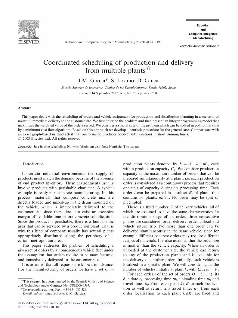
Thus, we can consider sik ¼ ei � tiik � tpi as the starttime of order i in plant k; lik ¼ ei � tiik the start time ofthe distribution of order i from plant k; and fik0 ¼ei þ tui þ trik0 he corresponding arrival time of thevehicle back to the plant k0: Fig. 1 shows graphicallythe process associated to activity of order i when it isprocessed in plant k and the vehicle returns to plant k0:

Moreover, each order i has a positive weight wi

reflecting the profit associated to serving it. A unit cost isassociated per unit travel time. Production unit costs areassumed to be the same for all plants, therefore onlydistribution costs are considered.

As we have a limited capacity in each plant, a fixednumber of vehicles available and orders have to beserved exactly at their due dates, it may happen that it isnot feasible to serve all orders. Hence, the objective is tomaximize the profit of the solution schedule consideringboth the weighted value of the served orders andtransportation costs.

The coordinated scheduling of production anddelivery is related to the following areas:

* Flow shop with parallel machines scheduling* Just-in-time (JIT) scheduling* No-wait scheduling.

When a single plant is considered [1,2], the probleminvolves a two-station flow shop with parallel machines(FSPM). The first station would be the productionplant, which is composed of a number of identicalmachines equal to the plant capacity. The second stationis composed of a number of identical machines equal tothe number of vehicles. Each job would correspond withthe production and delivery of each order. All jobs mustbe processed on each station in the same order. At thestation, a job can be processed on any machine. Severalworks have studied the FSPM with two stages (e.g. [3,4])although most of them consider the makespan asobjective function. In addition, when multiple produc-tion plants are considered, as in this paper, the problemis not longer related to FSPM because neither thenumber of resources nor the processing times in thesecond stage (i.e. the distribution phase) are constant.

From another point of view, the current interest in theJIT philosophy in industry has motivated the study ofscheduling problems where an ideal schedule is one inwhich all jobs finish exactly on their due dates. This can

Production Distributiontpi Delivery(tiik) Unload(tui) Return trip(trik')

sik lik ei fik

Fig. 1. Activity of order i:

be translated to a scheduling objective in several ways.The most general objective is to minimize the totalearliness and tardiness penalty [5]. However, there areother ways that may be appropriate to measure thegoodness of a schedule in a just-in-time environment.One of them, which is used in our problem, is tomaximize the weighted number of jobs that arecompleted exactly at their due dates. Only a few worksin the literature deal with scheduling problems with thisobjective. Thus, [6,7] study this problem on parallelidentical machines while [8] considers the objective ofmaximizing the number of on-time jobs (i.e. same weightfor all jobs) on a single machine. In all of these cases,jobs are available at the beginning of the schedulinghorizon, which differs from our problem.

Other type of scheduling problems related with thisJIT environment is the Fixed Job Scheduling Problem(FSP) [9,10]. FSP consists in scheduling a number ofjobs on identical parallel machines, each with a fixedstarting time, a fixed finishing time and a weight. Theobjective is to find an assignment of jobs to machineswith maximal total weight. This problem considers onlya single stage.

Finally, a specific feature of our problem is theexistence of no-wait constraints. No-wait schedulingproblems occurs in industrial environments in which aproduct must be processed from start to finish withoutany interruption. Hall and Sriskandarajah [11] presentsa survey of such type of scheduling problems, of whichthe most similar to our problem is [12], a two-stageFSPM with an objective function of maximizing theweighted value of jobs completed within the schedulinghorizon.

The paper is organized as follows. In Section 2, weformulate the problem as an integer linear programmingproblem. In Section 3, we study a particular case wherethe production capacity for every plant is larger than orequal to the number of available vehicles. That case isclose to real-world situations in which vehicles are themain constraint for the system performance. Moreover,the approach used for solving that case will be usedas base for the heuristic described in Section 4 forthe general case. With the objective of validating theproposed heuristic, we also describe a graph-based exactapproach. Using this exact method for solving largeproblems requires a great deal of memory and computa-tion time. Both the number of nodes and number of arcsgrow exponentially with problem size. Computationalcomparisons are described in Section 5 and finally,conclusions are drawn in Section 6.

2. Formulation

To formulate the problem we introduce a discretetime scale by dividing time into T time periods, where

ARTICLE IN PRESSJ.M. Garcia et al. / Robotics and Computer-Integrated Manufacturing 20 (2004) 191–198 193

t ¼ 1yT : For every plant kAK at every instanttAf1yTg; we define Sðt; kÞ ¼ fiAO : kAKi&sikpt&lik > tg as the set of orders whose productionprocesses in plant k overlap in instant t: Let dik andd 0

ik be the transportation cost from the customer i site toplant k and vice versa, respectively.

Our model incorporates the following decisionvariables:

xik ¼ 1 if order i is processed in plant k; 0 otherwise,8iAO; kAKi; zik ¼ 1 if the vehicle that serves order i

returns to plant k; 0 otherwise,8iAO; 8kAK ; ytk¼ number of available vehicles atinstant t in plant k; tAf1yTg:

MaxXn

i¼1

XkAKi

wixik �Xn

i¼1

XkAKi

dikxik þXn

i¼1

Xm

k¼1

d 0ikzik

!;

subject toXkAKi

xikr1 8iAO; ð1Þ

XkAKi

xik �Xm

k¼1

zik ¼ 0 8iAO; ð2Þ

y0k ¼ vk 8kAK ; ð3Þ

ytk ¼ y0k �X

i:likotf g

xik þX

i:fikrtf g

zik 8tA 1yTf g 8kAK ;

ð4ÞXi:lik¼tf g

xikrytk 8tA 1yTf g; 8kAK ; ð5Þ

XiASðt;kÞ

xikrCk 8kAKi; 8tA 1yTf g

xik; zikA 0; 1f g: ð6Þ

The objective function maximizes the profit obtainedwith the selected orders. Constraints (1) impose that anorder can just be processed in at most one plant.Constraints (2) ensure that after an order is served(unloaded), the vehicle must return to a productionplant. Constraints (3) establish the initial number ofvehicles at each plant. Constraints (4) compute thenumber of available vehicles at each plant in everyinstant t: Constraints (5) impose that an order i may beprocessed in plant k if there are available vehicles ininstant lik: Finally, constraints (6) assure that no morethan Ck orders are assigned to any time period in anyproduction plant.

3. A special case: unlimited production capacity

In this section, we consider a special case of theproblem in which the production capacity Ck in every

plant k is assumed as unlimited or, simply, greater thanor equal to the number of vehicles V : When VpCk;8kAK ; the problem becomes interesting since con-straints (6) do not impose any restriction and can beeliminated. That is, as V does not exceed the productioncapacity Ck in any plant k; there is enough capacity ineach plant to process all orders that may be distributedat any instant.

This special case can be modeled as a minimum costflow problem, which can be solved efficiently. Moreover,this case can be used to get an upper bound on theoptimal solution of the general problem. We will alsoshow how this minimum cost flow problem relates to themodel of the previous section.

The construction of the directed graph GðN;AÞ thatwe use to solve the problem can be described as follows:

For each order i we create a subgraph GiðNi;AiÞwhose paths reflect all the possible schedules for theorder. The set Ni consists of mi(possible originplants)+m(possible return plants)+2(start and end ofunload) nodes:

oi1; o

i2;y; oi

mi; ri

1; ri2;y; ri

m; si; ei:

The set Ai consists of the following arcs:ðoi

1; siÞ; ðoi2; siÞ;y; ðoi

mi; siÞ that represent the production

of order i in each plant kAKi and the later deliveryto the customer site. Costs of these arcs correspondwith transportation costs dik ðsi; eiÞ that represents theunload of order i: The weight of order i is represented asa negative cost �wi in this arc. ðei; ri

1Þ; ðei; ri2Þ;y; ðei; ri

mÞthat represent each possible return trip after order i isserved. The cost of each arc is the return cost d 0

ik

Besides a subgraph GiðNi;AiÞ for each order i; the graphGðN;AÞ is made up of the following nodes and arcs:

Nodes p1;y; pk;y; pm that have not incoming arcs,and are called supply nodes because each contains vkk ¼1ym units of flow that represent the number of vehiclesinitially at the plant. Each node pk is connected to everynode oi

s that represents the production of order i in plantk, kAKi; i ¼ 1yn:

Node t that has no outgoing arcs and is called thedemand node. All the nodes ri

k are i ¼ 1yn k ¼ 1ym

are connected to the node t with cost zero.Finally, there are arcs ðri

k; ojkÞ for those iaj for which

fikpljk: Note that if ðrik; o

jkÞAA; then order i and order j

can be scheduled for the same vehicle, which returns toplant k after serving order i; in such a manner that bothorders i and j are served just-in-time. The number ofarcs that can be created with this rule is less than orequal to mðn2 � nÞ=2:

All the arcs in G can carry one unit of flow since anorder can be served at most once. The number of nodesin G is less than or equal to m þ 2mn þ 2n þ 1: Thenumber of arcs is less than or equal to m2 þ 2mn þ n þmðn2 � nÞ=2: The optimal solution to the minimum costflow problem in G will obtain the orders to be processed.

ARTICLE IN PRESSJ.M. Garcia et al. / Robotics and Computer-Integrated Manufacturing 20 (2004) 191–198194

Obviously, an order i is processed if one unit of flowcirculates through subgraph Gi:

The optimal solution to this minimum cost flowproblem can be obtained by different algorithms. Theone we have used is the RELAX IV [13], in particularthe C++ implementation downloadable from [14].

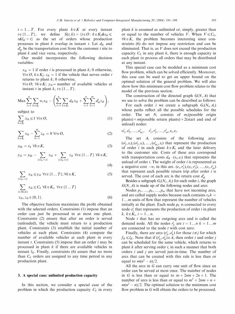
The following example illustrates how a problem canbe transformed to an instance of a minimum cost flowproblem. Graph G for the data presented in Table 1 isshown in Fig. 2. For this example we consider twoplants and three orders, assuming all the orders can beprocessed at any plant.

Using the algorithm RELAX IV with the weights,transportation costs and vehicles shown in Table 2, weobtain a flow of minimum cost (Fig. 3). This flow hastwo paths depicted by bold lines, each of whichcorresponds to the schedule of a vehicle. For thisexample, all the orders are served. Orders 1 and 2 fromplant 1 and order 2 from plant 2. A vehicle serves orders1 and 3 and the other vehicle serves order 2.

For the special case considered, the model presentedin the previous section, although using mathematicalnotation, corresponds to the minimum cost flowproblem described in this section:

* Variables xik represent flow in arcs ðoik; siÞ;

* Variables zik represent flow in arcs ðei; rikÞ;

* Variables ytk represent the calculation of flow thatcould circulate trough nodes oi

k at any instant ofthe scheduling. This calculation is represented in

Table 1

Example

i si1 si2 li1 li2 fi1 fi2

1 2 3 3 4 10 11

2 6 4 7 5 12 14

3 10 9 11 10 13 13

s1 e1

-w1

d11

d12

s2 e2

d22

p2

p1

s3 e3

t

d21

d31

d32

d'11

d'12

d'21

d'22

d'31

d'32

v1

v2

v1+ v2-w2

-w3

11o

12o

22o

21o

31o

32o

1

1r

32r

31r

22r

2

1r

1

2r

Fig. 2. Graph G for the example of Table 1.

the graph with the previous calculation of arcsðri

k; ojkÞ:

4. Two approaches for solving the general case

In this section we propose two different strategies forsolving the problem in the general case. The firststrategy uses an exact method to get the optimalsolution. The primary reason for developing thisgraph-based approach is that its results can usefullyguide the conclusions about the validity of the heuristicmethod that is described in Section 4.2.

4.1. A graph-based exact solution method

The approach we present is similar to a previouseffective graph-based method proposed for the sameproblem but with only one production plant [2]. Theapproach builds a graph G that collects all feasiblesolutions to the problem by means of an evaluationmethod of all feasible states in the scheduling of orders.The maximal weighted path from start node to end nodein G is the optimal solution to the problem.

The process can be described as follows: We considerthe events corresponding to the start of processing ofeach order i at each plant k; kAKi: Let P be the totalnumber of such events. The set ftp : p ¼ 1;y;Pg is usedto represent these events in chronological order. That is,

s1 e1

-105

6

s2 e2

4

p2

p1

s3 e3

t

6

6

4

4

4

3

5

5

4

1

1

2-12

-10

11o

12o

22o

21o

31o

32o

1

1r

32r

31r

22r

2

1r

1

2r

Fig. 3. A flow of minimum cost.

Table 2

Weights, costs and vehicles for the example of Table 1

i wi di1 di2 d 0i1 d 0

i2 v1 ¼ 1; v2 ¼ 1

1 10 5 6 4 4

2 12 6 4 3 5

3 10 6 4 5 4

ARTICLE IN PRESSJ.M. Garcia et al. / Robotics and Computer-Integrated Manufacturing 20 (2004) 191–198 195

ftp; p ¼ 1yPg ¼ fsik : i ¼ 1yn; k ¼ 1ym; kAKig andtp�1ptp for p ¼ 1yP: Therefore, Ppnm:

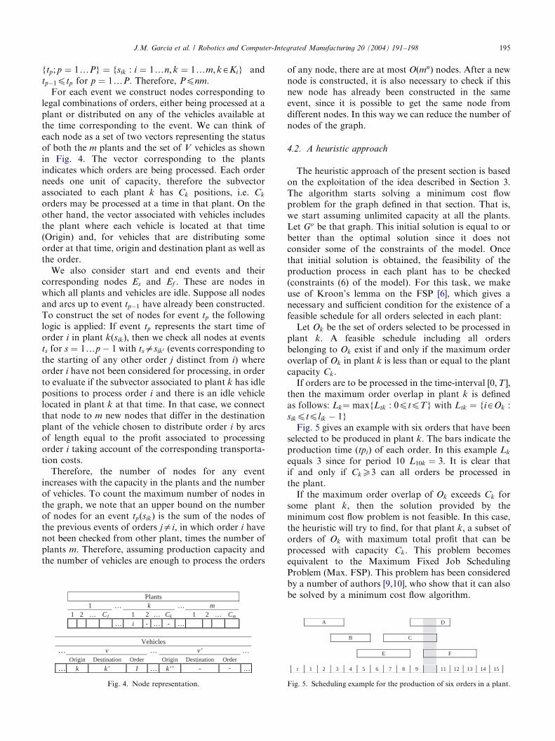
For each event we construct nodes corresponding tolegal combinations of orders, either being processed at aplant or distributed on any of the vehicles available atthe time corresponding to the event. We can think ofeach node as a set of two vectors representing the statusof both the m plants and the set of V vehicles as shownin Fig. 4. The vector corresponding to the plantsindicates which orders are being processed. Each orderneeds one unit of capacity, therefore the subvectorassociated to each plant k has Ck positions, i.e. Ck

orders may be processed at a time in that plant. On theother hand, the vector associated with vehicles includesthe plant where each vehicle is located at that time(Origin) and, for vehicles that are distributing someorder at that time, origin and destination plant as well asthe order.

We also consider start and end events and theircorresponding nodes Es and Ef : These are nodes inwhich all plants and vehicles are idle. Suppose all nodesand arcs up to event tp�1 have already been constructed.To construct the set of nodes for event tp the followinglogic is applied: If event tp represents the start time oforder i in plant kðsikÞ; then we check all nodes at eventsts for s ¼ 1yp � 1 with tsasik0 (events corresponding tothe starting of any other order j distinct from i) whereorder i have not been considered for processing, in orderto evaluate if the subvector associated to plant k has idlepositions to process order i and there is an idle vehiclelocated in plant k at that time. In that case, we connectthat node to m new nodes that differ in the destinationplant of the vehicle chosen to distribute order i by arcsof length equal to the profit associated to processingorder i taking account of the corresponding transporta-tion costs.

Therefore, the number of nodes for any eventincreases with the capacity in the plants and the numberof vehicles. To count the maximum number of nodes inthe graph, we note that an upper bound on the numberof nodes for an event tpðsikÞ is the sum of the nodes ofthe previous events of orders jai; in which order i havenot been checked from other plant, times the number ofplants m: Therefore, assuming production capacity andthe number of vehicles are enough to process the orders

Plants 1 k … m

1 2 … C1 1 2 … Ck 1 2 … Cm

… i - … - …

Vehicles … v … v’

Origin Destination Order Origin Destination Order

… k I … k’’ - - …

…

k’

…

Fig. 4. Node representation.

of any node, there are at most OðmnÞ nodes. After a newnode is constructed, it is also necessary to check if thisnew node has already been constructed in the sameevent, since it is possible to get the same node fromdifferent nodes. In this way we can reduce the number ofnodes of the graph.

4.2. A heuristic approach

The heuristic approach of the present section is basedon the exploitation of the idea described in Section 3.The algorithm starts solving a minimum cost flowproblem for the graph defined in that section. That is,we start assuming unlimited capacity at all the plants.Let Go be that graph. This initial solution is equal to orbetter than the optimal solution since it does notconsider some of the constraints of the model. Oncethat initial solution is obtained, the feasibility of theproduction process in each plant has to be checked(constraints (6) of the model). For this task, we makeuse of Kroon’s lemma on the FSP [6], which gives anecessary and sufficient condition for the existence of afeasible schedule for all orders selected in each plant:

Let Ok be the set of orders selected to be processed inplant k: A feasible schedule including all ordersbelonging to Ok exist if and only if the maximum orderoverlap of Ok in plant k is less than or equal to the plantcapacity Ck:

If orders are to be processed in the time-interval ½0;T �;then the maximum order overlap in plant k is definedas follows: Lk¼ maxfLtk : 0ptpTg with Ltk ¼ fiAOk :sikptplik � 1g

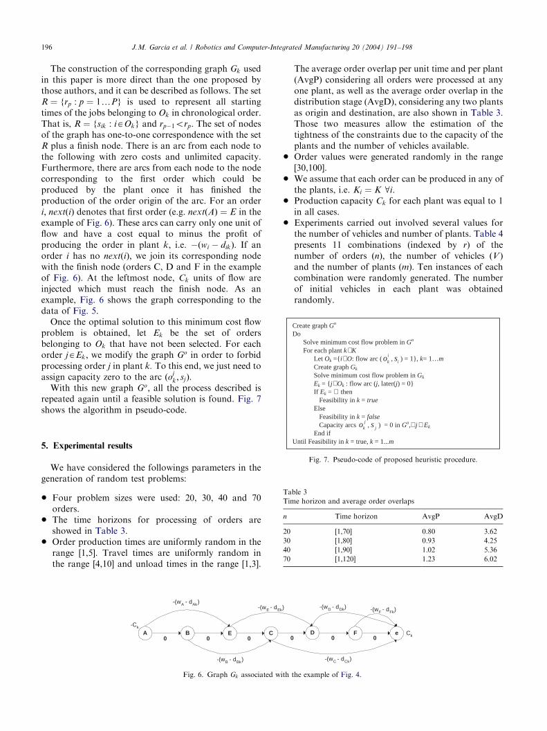
Fig. 5 gives an example with six orders that have beenselected to be produced in plant k: The bars indicate theproduction time ðtpiÞ of each order. In this example Lk

equals 3 since for period 10 L10k ¼ 3: It is clear thatif and only if CkX3 can all orders be processed inthe plant.

If the maximum order overlap of Ok exceeds Ck forsome plant k; then the solution provided by theminimum cost flow problem is not feasible. In this case,the heuristic will try to find, for that plant k; a subset oforders of Ok with maximum total profit that can beprocessed with capacity Ck: This problem becomesequivalent to the Maximum Fixed Job SchedulingProblem (Max. FSP). This problem has been consideredby a number of authors [9,10], who show that it can alsobe solved by a minimum cost flow algorithm.

A D

B C

D

E F

t 1 2 3 4 5 6 7 8 9 10 11 12 13 14 15

Fig. 5. Scheduling example for the production of six orders in a plant.

ARTICLE IN PRESS

Create graph Go

DoSolve minimum cost flow problem in Go

For each plant k ∈ KLet Ok ={i ∈ O: flow arc (

i

ko , is ) = 1}, k= 1…m Create graph Gk

Solve minimum cost flow problem in Gk

Ek = {j ∈ Ok : flow arc (j, later(j) = 0} If Ek = ∅ then

Feasibility in k = trueElse

J.M. Garcia et al. / Robotics and Computer-Integrated Manufacturing 20 (2004) 191–198196

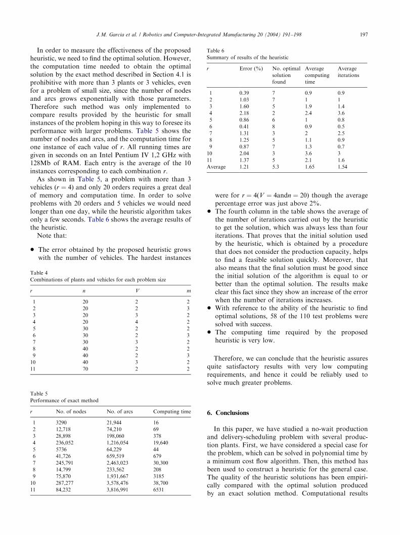
The construction of the corresponding graph Gk usedin this paper is more direct than the one proposed bythose authors, and it can be described as follows. The setR ¼ frp : p ¼ 1yPg is used to represent all startingtimes of the jobs belonging to Ok in chronological order.That is, R ¼ fsik : iAOkg and rp�1orp: The set of nodesof the graph has one-to-one correspondence with the setR plus a finish node. There is an arc from each node tothe following with zero costs and unlimited capacity.Furthermore, there are arcs from each node to the nodecorresponding to the first order which could beproduced by the plant once it has finished theproduction of the order origin of the arc. For an orderi; nextðiÞ denotes that first order (e.g. nextðAÞ ¼ E in theexample of Fig. 6). These arcs can carry only one unit offlow and have a cost equal to minus the profit ofproducing the order in plant k; i.e. �ðwi � dikÞ: If anorder i has no nextðiÞ; we join its corresponding nodewith the finish node (orders C, D and F in the exampleof Fig. 6). At the leftmost node, Ck units of flow areinjected which must reach the finish node. As anexample, Fig. 6 shows the graph corresponding to thedata of Fig. 5.

Once the optimal solution to this minimum cost flowproblem is obtained, let Ek be the set of ordersbelonging to Ok that have not been selected. For eachorder jAEk; we modify the graph Go in order to forbidprocessing order j in plant k. To this end, we just need toassign capacity zero to the arc ðoj

k; sjÞ:With this new graph Go; all the process described is

repeated again until a feasible solution is found. Fig. 7shows the algorithm in pseudo-code.

Table 3

Time horizon and average order overlaps

n Time horizon AvgP AvgD

20 [1,70] 0.80 3.62

30 [1,80] 0.93 4.25

40 [1,90] 1.02 5.36

70 [1,120] 1.23 6.02

Feasibility in k = falseCapacity arcs

j

ko , js ) = 0 in Go,∀ j ∈ Ek

End ifUntil Feasibility in k = true, k = 1...m

Fig. 7. Pseudo-code of proposed heuristic procedure.

5. Experimental results

We have considered the followings parameters in thegeneration of random test problems:

* Four problem sizes were used: 20, 30, 40 and 70orders.

* The time horizons for processing of orders areshowed in Table 3.

* Order production times are uniformly random in therange [1,5]. Travel times are uniformly random inthe range [4,10] and unload times in the range [1,3].

A B E C0 0 0

-(wA - dAk)

-(wB - dBk)

-(wE - dEk

-Ck

Fig. 6. Graph Gk associated w

The average order overlap per unit time and per plant(AvgP) considering all orders were processed at anyone plant, as well as the average order overlap in thedistribution stage (AvgD), considering any two plantsas origin and destination, are also shown in Table 3.Those two measures allow the estimation of thetightness of the constraints due to the capacity of theplants and the number of vehicles available.

* Order values were generated randomly in the range[30,100].

* We assume that each order can be produced in any ofthe plants, i.e. Ki ¼ K 8i:

* Production capacity Ck for each plant was equal to 1in all cases.

* Experiments carried out involved several values forthe number of vehicles and number of plants. Table 4presents 11 combinations (indexed by r) of thenumber of orders ðnÞ; the number of vehicles ðV Þand the number of plants ðmÞ: Ten instances of eachcombination were randomly generated. The numberof initial vehicles in each plant was obtainedrandomly.

D eF0 0 0

)

-(wC - dCk)

-(wD - dDk) -(wF - dFk)

Ck

ith the example of Fig. 4.

ARTICLE IN PRESS

Table 6

Summary of results of the heuristic

r Error (%) No. optimal

solution

found

Average

computing

time

Average

iterations

1 0.39 7 0.9 0.9

2 1.03 7 1 1

3 1.60 5 1.9 1.4

4 2.18 2 2.4 3.6

5 0.86 6 1 0.8

6 0.41 8 0.9 0.5

7 1.31 3 2 2.5

8 1.25 5 1.1 0.9

9 0.87 7 1.3 0.7

10 2.04 3 3.6 3

11 1.37 5 2.1 1.6

Average 1.21 5.3 1.65 1.54

J.M. Garcia et al. / Robotics and Computer-Integrated Manufacturing 20 (2004) 191–198 197

In order to measure the effectiveness of the proposedheuristic, we need to find the optimal solution. However,the computation time needed to obtain the optimalsolution by the exact method described in Section 4.1 isprohibitive with more than 3 plants or 3 vehicles, evenfor a problem of small size, since the number of nodesand arcs grows exponentially with those parameters.Therefore such method was only implemented tocompare results provided by the heuristic for smallinstances of the problem hoping in this way to foresee itsperformance with larger problems. Table 5 shows thenumber of nodes and arcs, and the computation time forone instance of each value of r: All running times aregiven in seconds on an Intel Pentium IV 1,2 GHz with128Mb of RAM. Each entry is the average of the 10instances corresponding to each combination r:

As shown in Table 5, a problem with more than 3vehicles ðr ¼ 4Þ and only 20 orders requires a great dealof memory and computation time. In order to solveproblems with 20 orders and 5 vehicles we would needlonger than one day, while the heuristic algorithm takesonly a few seconds. Table 6 shows the average results ofthe heuristic.

Note that:

* The error obtained by the proposed heuristic growswith the number of vehicles. The hardest instances

Table 4

Combinations of plants and vehicles for each problem size

r n V m

1 20 2 2

2 20 2 3

3 20 3 2

4 20 4 2

5 30 2 2

6 30 2 3

7 30 3 2

8 40 2 2

9 40 2 3

10 40 3 2

11 70 2 2

Table 5

Performance of exact method

r No. of nodes No. of arcs Computing time

1 3290 21,944 16

2 12,718 74,210 69

3 28,898 198,060 378

4 236,052 1,216,054 19,640

5 5736 64,229 44

6 41,726 659,519 679

7 245,791 2,463,023 30,300

8 14,799 233,562 208

9 75,870 1,931,667 3185

10 287,277 3,578,476 38,700

11 84,232 3,816,991 6531

were for r ¼ 4ðV ¼ 4andn ¼ 20Þ though the averagepercentage error was just above 2%.

* The fourth column in the table shows the average ofthe number of iterations carried out by the heuristicto get the solution, which was always less than fouriterations. That proves that the initial solution usedby the heuristic, which is obtained by a procedurethat does not consider the production capacity, helpsto find a feasible solution quickly. Moreover, thatalso means that the final solution must be good sincethe initial solution of the algorithm is equal to orbetter than the optimal solution. The results makeclear this fact since they show an increase of the errorwhen the number of iterations increases.

* With reference to the ability of the heuristic to findoptimal solutions, 58 of the 110 test problems weresolved with success.

* The computing time required by the proposedheuristic is very low.

Therefore, we can conclude that the heuristic assuresquite satisfactory results with very low computingrequirements, and hence it could be reliably used tosolve much greater problems.

6. Conclusions

In this paper, we have studied a no-wait productionand delivery-scheduling problem with several produc-tion plants. First, we have considered a special case forthe problem, which can be solved in polynomial time bya minimum cost flow algorithm. Then, this method hasbeen used to construct a heuristic for the general case.The quality of the heuristic solutions has been empiri-cally compared with the optimal solution producedby an exact solution method. Computational results

ARTICLE IN PRESSJ.M. Garcia et al. / Robotics and Computer-Integrated Manufacturing 20 (2004) 191–198198

indicate that the heuristic finds solutions of very goodquality in a short computation time.

References

[1] Garcia JM, Smith K, Lozano S, Guerrero F, Calle M. Production

and delivery scheduling problem with time windows. Proceedings

of the 30th International Conference on Computers and

Industrial Engineering, Publishing ZITI, Tynos Island, Greece,

2002. p. 263–8.

[2] Garcia JM, Smith K, Lozano S, Guerrero F. A comparison of

GRASP and an exact method for solving a production and

delivery scheduling problem. Hybrid information systems. In:

Abraham A, K .oppen M, editors. Advances in soft computing.

Heidelberg: Physica-Verlag; 2002. p. 431–47.

[3] Gupta JND. Two stage hybrid flow-shop scheduling problem.

J Oper Res 1988;29/7:1489–502.

[4] Haouari M, M’Hallah R. Heuristic algorithms for the two-stage

hybrid flowshop problem. Oper Res Lett 1997;21:43–53.

[5] Baker KR, Scudder GD. Sequencing with earliness and tardiness

penalties: a review. Oper Res 1990;38:22–36.

[6] Hiraishi K, Levner E, Vlach M. Scheduling of parallel identical

machines to maximize the weighted number of just-in-time jobs.

Comput Oper Res 2002;29:841–8.

[7] Lann A, Mosheiov G. A note on the maximum number of on time

jobs on parallel identical machines. Comput Oper Res 2002;30:

1745–9.

[8] Lann A, Mosheiov G. Single machine scheduling to minimize the

number of early and tardy jobs. Comput Oper Res 1996;8:765–8.

[9] Arking EM, Silverberg EB. Scheduling jobs with fixed start and

end times. Discrete Appl Math 1987;18:1–8.

[10] Kroon LG, Salomon M, Van Wassenhove LN. Exact and

approximation algorithms for the operational fixed interval

scheduling problem. Eur J Oper Res 1995;82:190–205.

[11] Hall NG, Sriskandarajah C. A survey of machine scheduling

problems with blocking and no-wait in process. Oper Res 1996;

44:510–25.

[12] Ramudhin A, Ratliff HD. Generating daily production schedules

in process industries. IIE Trans 1995;27:646–56.

[13] Bertsekas D, Tseng P. Relaxation methods for minimum cost for

ordinary and generalized network flow problems. Oper Res

1988;36:93–114.

[14] Frangioni A. http://www.di.unipi.it/di/groups/optimize/Software/

index.html (November, 2002).